AdaScale SGD: A User-Friendly Algorithm for Distributed Training

Abstract

When using large-batch training to speed up stochastic gradient descent, learning rates must adapt to new batch sizes in order to maximize speed-ups and preserve model quality. Re-tuning learning rates is resource intensive, while fixed scaling rules often degrade model quality. We propose AdaScale SGD, an algorithm that reliably adapts learning rates to large-batch training. By continually adapting to the gradient’s variance, AdaScale automatically achieves speed-ups for a wide range of batch sizes. We formally describe this quality with AdaScale’s convergence bound, which maintains final objective values, even as batch sizes grow large and the number of iterations decreases. In empirical comparisons, AdaScale trains well beyond the batch size limits of popular “linear learning rate scaling” rules. This includes large-batch training with no model degradation for machine translation, image classification, object detection, and speech recognition tasks. AdaScale’s qualitative behavior is similar to that of “warm-up” heuristics, but unlike warm-up, this behavior emerges naturally from a principled mechanism. The algorithm introduces negligible computational overhead and no new hyperparameters, making AdaScale an attractive choice for large-scale training in practice.

0.173in

1 Introduction

Large datasets and large models underlie much of the recent success of machine learning. Training such models is time consuming, however, often requiring days or even weeks. Faster training enables consideration of more data and models, which expands the capabilities of machine learning.

Stochastic gradient descent and its variants are fundamental training algorithms. During each iteration, SGD applies a small and noisy update to the model, based on a stochastic gradient. By applying thousands of such updates in sequence, a powerful model can emerge over time.

To speed up SGD, a general strategy is to improve the signal-to-noise ratio of each update, i.e., reduce the variance of the stochastic gradient. Some tools for this include SVRG-type gradient estimators (Johnson & Zhang, 2013; Defazio et al., 2014) and prioritization of training data via importance sampling (Needell et al., 2014; Zhao & Zhang, 2015). Data parallelism—our focus in this work—is perhaps the most powerful of such tools. By processing thousands of training examples for each gradient estimate, distributed systems can drastically lower the gradient’s variance. Only the system’s scalability, not the algorithm, limit the variance reduction.

Smaller variances alone, however, typically result in unimpressive speed-ups. To fully exploit the noise reduction, SGD must also make larger updates, i.e., increase its learning rate parameter. While this fact applies universally (including for SVRG (Johnson & Zhang, 2013), data parallelism (Goyal et al., 2017), and importance sampling (Johnson & Guestrin, 2018)), the precise relationship between variance and learning rates remains poorly quantified.

For this reason, practitioners often turn to heuristics in order to adapt learning rates. This applies especially to distributed training, for which case “fixed scaling rules” are standard but unreliable strategies. For example, Goyal et al. (2017) popularized “linear learning rate scaling,” which succeeds in limited cases (Krizhevsky, 2014; Devarakonda et al., 2017; Jastrzębski et al., 2018; Smith et al., 2018; Lin et al., 2019). For other problems or greater scales, however, linear scaling leads to poor model quality and even divergence—a result known both in theory (Yin et al., 2018; Jain et al., 2018; Ma et al., 2018) and in practice (Goyal et al., 2017).

In this work, we introduce AdaScale SGD, an algorithm that more reliably adjusts learning rates for large-batch training. AdaScale achieves speed-ups that depend naturally on the gradient’s variance before it is decreased—nearly perfect linear speed-ups in cases of large variance, and smaller speed-ups otherwise. For contrast, we also show that as batch sizes increase, linear learning rate scaling progressively degrades model quality, even when including “warm-up” heuristics (Goyal et al., 2017) and additional training iterations.

AdaScale						Linear scaling
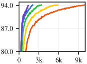
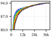
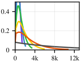
Val. Acc (%)		Val. Acc (%)		Learning rate ${\eta_{t}}$		Val. Acc (%)
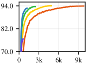
	Iteration		Scale-invariant itr.		Iteration		Iteration

Figure 1: Motivating results. For $\mathtt{cifar10}$, AdaScale automatically adapts to many scales $S$ (the number of parallel batches), preserving model quality. When plotted in terms of “scale-invariant” iterations, training curves align closely. With AdaScale, warm-up behavior emerges naturally when adapting a simple learning rate schedule (exponential decay) to scale $S$ (plot cropped to show behavior). Meanwhile, linear scaling (with warm-up) degrades model quality as batch sizes increase.

AdaScale makes large-batch training significantly more user-friendly. Without changing the algorithm’s inputs (such as learning rate schedule), AdaScale can adapt to vastly different batch sizes with large speed-ups and near-identical model quality. This has two important implications: (i) AdaScale improves the translation of learning rates to greater amounts of parallelism, which simplifies scaling up tasks or adapting to dynamic resource availability; and (ii) AdaScale works with simple learning rate schedules at scale, eliminating the need for warm-up. Qualitatively, AdaScale and warm-up have similar effects on learning rates, but with AdaScale, the behavior emerges from a principled and adaptive strategy, not hand-tuned parameters.

We perform large-scale empirical evaluations on five training benchmarks. Tasks include image classification, machine translation, object detection, and speech recognition. The results align remarkably well with our theory, as AdaScale systematically preserves model quality across many batch sizes. This includes training ImageNet with batch size 32k and Transformer with 262k max tokens per batch.

The ideas behind AdaScale are not limited to distributed training, but instead apply to any estimator that reduces the gradient’s variance. To provide context for the remaining sections, Figure 1 includes results from an experiment using CIFAR-10 data. These results illustrate AdaScale’s scaling behavior, the qualitative impact on learning rates, and a failure case for the linear scaling rule.

2 Problem formulation

We focus on quickly and approximately solving

$$\mathrm{minimize}_{\mathbf{w}\in\mathbb{R}^{d}}\ F(\mathbf{w}):=\mathbb{E}_{\mathbf{x}\sim\mathcal{X}}\left[f(\mathbf{w},\mathbf{x})\right]\,.$$ (1)

Here $\mathbf{w}$ parameterizes a machine learning model, while $\mathcal{X}$ denotes a distribution over batches of training data. We assume that $F$ and $f$ are differentiable and that $\mathbb{E}_{\mathbf{x}\sim\mathcal{X}}\left[\nabla_{\mathbf{w}}f(\mathbf{w},\mathbf{x})\right]=\nabla F(\mathbf{w})$.

SGD is a fundamental algorithm for solving Problem 1. Let $\mathbf{w}_{t}$ denote the model parameters when iteration $t$ begins. SGD samples a batch $\mathbf{x}_{t}\sim\mathcal{X}$ and computes the gradient $\mathbf{g}_{t}\leftarrow\nabla_{\mathbf{w}}f(\mathbf{w}_{t},\mathbf{x}_{t})$, before applying the update

$$\mathbf{w}_{t+1}\leftarrow\mathbf{w}_{t}-{\eta_{t}}\mathbf{g}_{t}\,.$$ (2)

Here ${\eta_{t}}$ is the learning rate. Given a learning rate schedule $\mathtt{lr}\,:\,\mathbb{Z}_{\geq 0}\rightarrow\mathbb{R}_{>0}$, SGD defines ${\eta_{t}}=\mathtt{lr}\textrm{(}t\textrm{)}$. For our experiments in §4, $\mathtt{lr}$ is an exponential decay or step decay function. SGD completes training after $T$ iterations.

To speed up SGD, we can process multiple batches in parallel. Algorithm 1 defines a “scaled SGD” algorithm. At scale $S$, we sample $S$ independent batches per iteration. After computing the gradient for each batch in parallel, the algorithm synchronously applies the mean of these gradients (in place of $\mathbf{g}_{t}$ in (2)) when updating the model.

As $S$ increases, scaled SGD generally requires fewer iterations to train a model. But how much speed-up should we expect, especially as $S$ becomes large? Moreover, how do we adapt learning rates in order to realize this speed-up? Practitioners usually answer these questions with one or two approaches: (i) trial-and-error parameter tuning, which requires significant time and specialized knowledge, or (ii) fixed scaling rules, which work well for some problems, but result in poor model quality for many others.

3 AdaScale SGD algorithm

In this section, we introduce AdaScale. We can interpret AdaScale as a per-iteration interpolation between two simple rules for scaling the learning rate. For each of these rules, we first consider an extreme problem setting for which the rule behaves ideally. With this understanding, we then define AdaScale and provide theoretical results. Finally, we discuss approximations needed for a practical implementation.

3.1 Intuition from extreme cases of gradient variance

Algorithm 1 Scaled SGD

$\mathtt{Scaled\_SGD}$$S$, $\mathtt{lr}$, $T$, $\mathcal{X}$, $f$, $\mathbf{w}_{0}$$t=0,1,2,\ldots,T-1$$\bar{\mathbf{g}}_{t}\leftarrow\mathtt{compute\_gradient}\textrm{(}\mathbf{w}_{t},S,\mathcal{X},f\textrm{)}$${\eta_{t}}\leftarrow\mathtt{lr}\textrm{(}t\textrm{)}$$\mathbf{w}_{t+1}\leftarrow\mathbf{w}_{t}-{\eta_{t}}\bar{\mathbf{g}}_{t}$return$\mathbf{w}_{T}$$\mathtt{compute\_gradient}$$\mathbf{w}_{t}$, $S$, $\mathcal{X}$, $f$in parallel for$i=1,\ldots,S$do$\mathbf{x}^{(i)}\leftarrow\mathtt{sample\_batch}(\mathcal{X})$$\mathbf{g}^{(i)}\leftarrow\nabla_{\mathbf{w}}f(\mathbf{w}_{t},\mathbf{x}^{(i)})$return$\tfrac{1}{S}\sum_{i=1}^{S}\mathbf{g}^{(i)}$

Algorithm 2 AdaScale SGD

$\mathtt{Ada\-Scale{}}$$S$, $\mathtt{lr}$, $T_{\mathrm{SI}}$, $\mathcal{X}$, $f$, $\mathbf{w}_{0}$initialize$\tau_{0}\leftarrow 0$; $t\leftarrow 0$$\tau_{t}<T_{\mathrm{SI}}$$\bar{\mathbf{g}}_{t}\leftarrow\mathtt{compute\_gradient}\textrm{(}\mathbf{w}_{t},S,\mathcal{X},f\textrm{)}$# Compute “gain” $r_{t}\in[1,S]$ (see (3) and §3.4):$r_{t}\leftarrow\frac{\mathbb{E}_{\mathbf{w}_{t}}\left[\sigma_{\mathbf{g}}^{2}(\mathbf{w}_{t})+\mu_{\mathbf{g}}^{2}(\mathbf{w}_{t})\right]}{\mathbb{E}_{\mathbf{w}_{t}}\left[\tfrac{1}{S}\sigma_{\mathbf{g}}^{2}(\mathbf{w}_{t})+\mu_{\mathbf{g}}^{2}(\mathbf{w}_{t})\right]}$${\eta_{t}}\leftarrow r_{t}\cdot\mathtt{lr}\textrm{(}\lfloor\tau_{t}\rfloor\textrm{)}$$\mathbf{w}_{t+1}\leftarrow\mathbf{w}_{t}-{\eta_{t}}\bar{\mathbf{g}}_{t}$$\tau_{t+1}\leftarrow\tau_{t}+r_{t}$; $t\leftarrow t+1$return$\mathbf{w}_{t}$

To help introduce AdaScale, we first consider two simple “scaling rules.” A scaling rule translates training parameters (such as learning rates) to large-batch settings:

Definition 1.

Consider a learning rate schedule $\mathtt{lr}_{1}$ and total steps $T_{1}$ for single-batch training (i.e., Algorithm 1 with $S=1$). Given a scale $S$, a scaling rule maps $(S,\mathtt{lr}_{1},T_{1})$ to parameters $(\mathtt{lr}_{S},T_{S})$ for training at scale $S$.

One scaling rule is identity scaling, which keeps training parameters unchanged for all $S$:

Definition 2.

The identity scaling rule defines $T_{S}=T_{1}$ and $\mathtt{lr}_{S}=\mathtt{lr}_{1}$.

Note that this rule has little practical appeal, since it fails to reduce the number of training iterations. A more popular scaling rule is linear learning rate scaling:

Definition 3.

The linear scaling rule defines $T_{S}=\lceil T_{1}/S\rceil$ and $\mathtt{lr}_{S}(t)=S\cdot\mathtt{lr}_{1}(St)$.

Conceptually, linear scaling treats SGD as a perfectly parallelizable algorithm. If true, applying updates from $S$ batches in parallel achieves the same result as doing so in sequence.

For separate special cases of Problem 1, the identity and linear scaling rules maintain training effectiveness for all $S$. To show this, we first define the gradient variance quantities

$$\begin{array}[]{c}\bm{\Sigma}_{\mathbf{g}}(\mathbf{w})=\mathrm{cov}_{\mathbf{x}\sim\mathcal{X}}(\nabla_{\mathbf{w}}f(\mathbf{w},\mathbf{x}),\nabla_{\mathbf{w}}f(\mathbf{w},\mathbf{x}))\,,\\ \\[-8.00003pt] \text{and}\quad\sigma_{\mathbf{g}}^{2}(\mathbf{w})=\mathrm{tr}(\bm{\Sigma}_{\mathbf{g}}(\mathbf{w}))\,.\end{array}$$

In words, $\sigma_{\mathbf{g}}^{2}(\mathbf{w})$ sums the variances of each entry in $\nabla_{\mathbf{w}}f(\mathbf{w},\mathbf{x})$. Data parallelism fundamentally impacts SGD by reducing this variance.

We first consider the case of deterministic gradients, i.e., $\sigma_{\mathbf{g}}^{2}(\mathbf{w})=0$. Here identity scaling preserves model quality:

Proposition 1 (Identity scaling for zero variance).

Let $\mathbf{w}^{(1)}$ denote the result of single batch training, and let $\mathbf{w}^{(S)}$ denote the result of scaled training after identity scaling. If $\sigma_{\mathbf{g}}^{2}(\mathbf{w})=0$ for all $\mathbf{w}\in\mathbb{R}^{d}$, then $F(\mathbf{w}^{(1)})=F(\mathbf{w}^{(S)})$.

Although identity scaling does not speed up training, Proposition 1 is important for framing the impact of increasing batch sizes. If the gradient variance is “small,” then we cannot expect large gains from scaling up training—further reducing the variance has little effect on $\bar{\mathbf{g}}_{t}$. With “large” variance, however, the opposite is true:

Proposition 2 (Linear scaling for large variance).

Consider any learning rate $\eta$ and training duration $T$. For some fixed covariance matrix $\bm{\Sigma}\in\mathbb{S}^{d}_{>0}$ and $\nu\in\mathbb{Z}_{>0}$, assume $\nabla_{\mathbf{w}}f(\mathbf{w},\mathbf{x})\sim\mathcal{N}(\nabla F(\mathbf{w}),\nu\bm{\Sigma})$. Let $\mathtt{lr}_{1}(t)=\nu^{-1}\eta$ and $T_{1}=\nu T$. Define $\mathbf{w}^{(1)}$ as the result of single batch training and $\mathbf{w}^{(S)}$ as the result of scaled training after linear scaling. Then $\mathbb{E}\left[F(\mathbf{w}^{(1)})\right]=\mathbb{E}\left[F(\mathbf{w}^{(S)})\right]$ in the limit $\nu\rightarrow+\infty$.

In simpler terms, linear scaling leads to perfect linear speed-ups in the case of very large gradient variance (as well as small learning rates and many iterations, to compensate for this variance). Since increasing $S$ decreases variance, it is natural that scaling yields large speed-ups in this case.

In practice, the gradient’s variance is neither zero nor infinite, and both identity and linear scaling may perform poorly. Moreover, the gradient’s variance does not remain constant throughout training. A practical algorithm, it seems, must continually adapt to the state of training.

3.2 AdaScale definition

AdaScale, defined in Algorithm 2, adaptively interpolates between identity and linear scaling, based on the expectation of the gradient’s variance. During iteration $t$, AdaScale multiplies the learning rate by a “gain ratio” $r_{t}\in[1,S]$:

$${\eta_{t}}=r_{t}\cdot\mathtt{lr}\textrm{(}\lfloor\tau_{t}\rfloor\textrm{)}\,.$$

Here we define $\tau_{t}=\sum_{t^{\prime}=0}^{t-1}r_{t^{\prime}}$—the scale-invariant iteration. The idea is that iteration $t$ performs the equivalent of $r_{t}$ single-batch iterations, and $\tau_{t}$ accumulates this progress. AdaScale concludes when $\tau_{t}\geq T_{\mathrm{SI}}$, where $T_{\mathrm{SI}}$ is the “total scale-invariant iterations.” Since $r_{t}\in[1,S]$, AdaScale requires at least $\lceil T_{\mathrm{SI}}/S\rceil$ and at most $T_{\mathrm{SI}}$ iterations. For practical problem settings, this training duration often falls closer to $\lceil T_{\mathrm{SI}}/S\rceil$ than $T_{\mathrm{SI}}$ (as we see later in §4).

The identity and linear rules correspond to two special cases of AdaScale. If $r_{t}=1$ for all $t$, the algorithm equates to SGD with identity scaling. Similarly, if $r_{t}=S$ for all $t$, we have linear scaling. Thus, §3.1 suggests setting $r_{t}\approx 1$ when $\sigma_{\mathbf{g}}^{2}(\mathbf{w}_{t})$ is small and $r_{t}\approx S$ when this variance is large. Introducing the notation $\mu_{\mathbf{g}}^{2}(\mathbf{w}_{t})=\left\|\nabla F(\mathbf{w}_{t})\right\|^{2}$, AdaScale achieves this by defining

$$r_{t}=\frac{\mathbb{E}_{\mathbf{w}_{t}}\left[\sigma_{\mathbf{g}}^{2}(\mathbf{w}_{t})+\mu_{\mathbf{g}}^{2}(\mathbf{w}_{t})\right]}{\mathbb{E}_{\mathbf{w}_{t}}\left[\tfrac{1}{S}\sigma_{\mathbf{g}}^{2}(\mathbf{w}_{t})+\mu_{\mathbf{g}}^{2}(\mathbf{w}_{t})\right]}\,.$$ (3)

Here there are expectations both with respect to the batch distribution $\mathcal{X}$ (as part of the variance term, $\sigma_{\mathbf{g}}^{2}(\mathbf{w}_{t})$) and with respect to the distribution over training trajectories. A practical implementation requires estimating $r_{t}$, and we describe a procedure for doing so in §3.4. Interestingly, since $\mathbb{E}_{\mathbf{w}_{t}}\left[\mu_{\mathbf{g}}^{2}(\mathbf{w}_{t})\right]$ decreases toward zero with progress toward convergence, we find empirically that $r_{t}$ often gradually increases during training, resulting in a “warm-up” effect on the learning rate (see §4). In addition to this intuitive behavior, (3) has a more principled justification. In particular, this $r_{t}$ ensures that as $S$ increases, ${\eta_{t}}\mathbb{E}[\mu_{\mathbf{g}}^{2}(\mathbf{w}_{t})]$ and ${\eta_{t}}^{2}\mathbb{E}[\|\bar{\mathbf{g}}_{t}\|^{2}]$ increase multiplicatively by $r_{t}$. This leads to the convergence bound for AdaScale that we next present.

Table 1: Overview of training benchmarks.

Name	Task	Model	Dataset	Metric
$\mathtt{cifar10}$	Image classification	ResNet-18 (v2)	CIFAR-10	Top-1 accuracy (%)
$\mathtt{imagenet}$	Image classification	ResNet-50 (v1)	ImageNet	Top-1 accuracy (%)
$\mathtt{speech}$	Speech recognition	Deep speech 2	LibriSpeech	Word accuracy (%)
$\mathtt{transformer}$	Machine translation	Transformer base	WMT-2014	BLEU
$\mathtt{yolo}$	Object detection	YOLOv3	PASCAL VOC	mAP (%)

3.3 Theoretical results

We now present convergence bounds that describe the speed-ups from AdaScale. Even as the batch size increases, AdaScale’s bound converges to the same objective value. We also include an analogous bound for linear scaling.

Let us define $F^{*}=\min_{\mathbf{w}}F(\mathbf{w})$. Our analysis requires a few assumptions that are typical of SGD analysis of non-convex problems (see, for example, (Lei et al., 2017; Yuan et al., 2019)):

Assumption 1 ($\alpha$-Polyak-Łojasiewicz).

For some $\alpha>0$, $F(\mathbf{w})-F^{*}\leq\tfrac{1}{2\alpha}\left\|\nabla F(\mathbf{w})\right\|^{2}$ for all $\mathbf{w}$.

Assumption 2 ($\beta$-smooth).

For some $\beta>0$, we have $\|\nabla F(\mathbf{w})-\nabla F(\mathbf{w}^{\prime})\|\leq\beta\|\mathbf{w}-\mathbf{w}^{\prime}\|$ for all $\mathbf{w}$, $\mathbf{w}^{\prime}$.

Assumption 3 (Bounded variance).

There exists a $V\geq 0$ such that $\sigma_{\mathbf{g}}^{2}(\mathbf{w})\leq V$ for all $\mathbf{w}$.

We emphasize that we do not assume convexity. The PL condition, which is perhaps the strongest of the assumptions, is proven to hold for some nonlinear neural networks (Charles & Papailiopoulos, 2018).

We consider constant $\mathtt{lr}$ schedules, which result in simple and instructive bounds. Furthermore, constant learning rate schedules provide reasonable results for many deep learning problems (Sun, 2019). To provide context for the AdaScale bound, we first present a result for single-batch training:

Theorem 1 (Single-batch SGD bound).

Given Assumptions 1, 2, 3 and $\eta\in(0,2\beta^{-1})$, consider Algorithm 1 with $S=1$ and $\mathtt{lr}\textrm{(}t\textrm{)}=\eta$. Defining $\gamma=\eta\alpha(2-\eta\beta)$ and $\Delta=\tfrac{1}{2\gamma}\eta^{2}\beta V$, we have

$$\mathbb{E}\left[F(\mathbf{w}_{T})-F^{*}\right]\leq(1-\gamma)^{T}\left[F(\mathbf{w}_{0})-F^{*}\right]+\Delta\,.$$

The bound describes two important characteristics of the single-batch algorithm. First, the suboptimality converges in expectation to at most $\Delta$. Second, convergence to $\Delta+\epsilon$ requires at most $\lceil\log((F(\mathbf{w}_{0})-F^{*})\epsilon^{-1})/\log((1-\gamma)^{-1})\rceil$ iterations. We note similar bounds exist, under a stronger variance assumption (Karimi et al., 2016; Reddi et al., 2016; De et al., 2017; Yin et al., 2018).

Importantly, our AdaScale bound converges to this same $\Delta$ for all practical values of $S$:

Theorem 2 (AdaScale bound).

Define $\gamma$, $\Delta$ as in Theorem 1. Given Assumptions 1, 2, 3, $S\leq\gamma^{-1}$, and $\eta\in(0,2\beta^{-1})$, define $T$ as the total iterations of Algorithm 2 with $\mathtt{lr}\textrm{(}t\textrm{)}=\eta$ and scale $S$. Denoting $\bar{r}=\tfrac{1}{T}\sum_{t=0}^{T-1}r_{t}$, we have

$$\mathbb{E}\left[F(\mathbf{w}_{T})-F^{*}\right]\leq(1-\gamma)^{\bar{r}T}\left[F(\mathbf{w}_{0})-F^{*}\right]+\Delta\,.$$

This bound is remarkably similar to that of Theorem 1. Like single-batch SGD, the expected suboptimality converges to at most $\Delta$, but AdaScale achieves this for many batch sizes. Also, AdaScale reduces the total training iterations by a factor $\bar{r}$, the average gain. That is, AdaScale requires at most $\lceil\bar{r}^{-1}\log((F(\mathbf{w}_{0})-F^{*})\epsilon^{-1})/\log((1-\gamma)^{-1})\rceil$ iterations to converge to objective value $\Delta+\epsilon$.

Finally, we provide an analogous bound for linear scaling:

Theorem 3 (Bound for linear scaling rule).

Define $\gamma$ and $\Delta$ as in Theorem 1. Given $\eta\in(0,2(S\beta)^{-1})$ and Assumptions 1, 2, 3, consider Algorithm 1 with $\mathtt{lr}\textrm{(}t\textrm{)}=S\eta$. Defining $\xi(S)=(2-\eta\beta)/(2-S\eta\beta)$ and $F_{0}=F(\mathbf{w}_{0})$, we have

$$\mathbb{E}\left[F(\mathbf{w}_{T})-F^{*}\right]\leq\left(1-\tfrac{\gamma}{\xi(S)}\right)^{ST}\left[F_{0}-F^{*}\right]+{\xi(S)}\cdot\Delta\,.$$

Note $\xi(S)\geq 1$, and this function increases monotonically with $S$ (until an asymptote at $S=2(\eta\beta)^{-1}$). Thus, unlike in Theorem 2, the bound converges to a value that increases with $S$. This means that compared to AdaScale, linear scaling often leads to worse model quality and greater risk of divergence, especially for large $S$. We observe this behavior throughout our empirical comparisons in §4.

Finally, we note Theorem 2 requires $S\leq\gamma^{-1}$—for reasonably small $\eta$, this is similar to the stricter constraint $S\leq(2\eta\alpha)^{-1}$. Meanwhile, Theorem 3 requires that $S\leq 2(\eta\beta)^{-1}$. Compared to the constraint for AdaScale, this constraint is typically much stricter, since $\alpha\leq\beta$ (and $\alpha\ll\beta$ if the Hessian’s eigenspectrum contains large outlier values, which has been observed in practice for nerual networks (Sagun et al., 2017; Ghorbani & Krishnan, 2019)). It is also worth noting that if $\gamma$ is large enough that $S\geq\gamma^{-1}$, then training at smaller scales converges quickly (due to Theorem 1), and large batch sizes are likely unnecessary.

3.4 Practical considerations

	$\mathtt{imagenet}$, $S$$=$16	$\mathtt{imagenet}$, $S$$=$128	$\mathtt{cifar10}$, $S$$=$8
Gain ratio $r_{t}$
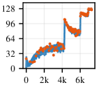
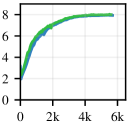
	Iteration $t$	Iteration $t$	Iteration $t$

Figure 2: Gain ratios. Plots compare various $r_{t}$ estimates. In practice, AdaScale uses online estimates from a single training trajectory. We compare to offline estimates (using 1000 batches). We also compare to online estimates that use five independent trajectories (tied only by their shared gain estimates) to average gradient moment estimates across trajectories during each iteration. The values align closely. For $\mathtt{imagenet}$, abrupt changes align with $\mathtt{lr}$ step changes.

A practical AdaScale implementation must efficiently approximate the gain ratio $r_{t}$ for all iterations. Fortunately, the per-batch gradients $\mathbf{g}_{t}^{(1)},\ldots,\mathbf{g}_{t}^{(S)}$ and aggregated gradient $\bar{\mathbf{g}}_{t}$ are readily available in distributed SGD algorithms. This makes approximating $r_{t}$ straightforward, since in addition to (3), we can express $r_{t}$ as the ratio of expectations

$$r_{t}=\frac{\mathbb{E}[\tfrac{1}{S}\sum_{i=1}^{S}\|\mathbf{g}_{t}^{(i)}\|^{2}]}{\mathbb{E}[\|\bar{\mathbf{g}}_{t}\|^{2}]}\,.\vspace{-0.1em}{}\vspace{-0.1em}{}\vspace{-0.1em}{}$$

Here we take the expectation over all randomness of the algorithm (both current and prior batches).

To estimate the gain, we recommend tracking moving averages of $\tfrac{1}{S}\sum_{i=1}^{S}\|\mathbf{g}_{t}^{(i)}\|^{2}$ and ${\|\bar{\mathbf{g}}_{t}\|^{2}}$ across iterations. Denoting these averages by $m_{1}$ and $m_{2}$, respectively, we can estimate the gain as $\hat{r}_{t}=\tfrac{m_{1}+\epsilon}{m_{2}+\epsilon}$. Here $\epsilon$ is a small constant, such as $10^{-6}$, for numerical stability.

For our empirical results, we use exponential moving averages with parameter $\theta=\max\{1-S/1000,0\}$, where $\theta=0$ results in no averaging. We find that AdaScale is robust to the choice of $\theta$, and we provide evidence of this in Appendix C. When ensuring numerical stability, the implementation for this work also uses an alternative to our recommendation of adding $\epsilon$ to $m_{1}$ and $m_{2}$ (see Appendix B for details). Our recommended strategy simplifies gain estimation but should not significantly affect results, since usually ${\|\bar{\mathbf{g}}_{t}\|^{2}}\gg\epsilon$ in practice.

Figure 2 verifies the usefulness of our estimator by comparing AdaScale’s estimates to improved (but impractical) ones. Moving averages (i) add robustness to estimation variance and (ii) incorporate multiple points from the optimization space. For (ii), we ideally would use points from independent training trajectories, but this is impractical. Even so, Figure 2 suggests that estimates from single and multiple trajectories can align closely. We note that numerous prior works—for example, (Schaul et al., 2013; Kingma & Ba, 2015; McCandlish et al., 2018)—have relied on similar moving averages to estimate gradient moments.

One final practical consideration is the momentum parameter $\rho$ when using AdaScale with momentum-SGD. The performance of momentum-SGD depends less critically on $\rho$ than the learning rate (Shallue et al., 2019). For this reason, AdaScale often performs well if $\rho$ remains constant across scales and iterations. This approach to momentum scaling has also succeeded in prior works involving the linear scaling rule (Goyal et al., 2017; Smith et al., 2018).

$\mathtt{imagenet}$
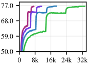
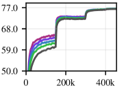
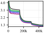
Val. Acc (%)		Val. Acc (%)		Training loss		Learning rate ${\eta_{t}}$
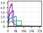
	Iteration $t$		$S$-invariant iteration $\tau_{t}$		$S$-invariant iteration $\tau_{t}$		Iteration $t$
$\mathtt{speech}$
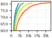
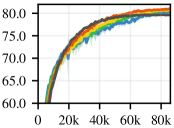
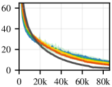
Val. WAcc (%)		Val. WAcc (%)		Training loss		Learning rate ${\eta_{t}}$
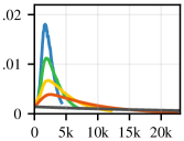
	Iteration $t$		$S$-invariant iteration $\tau_{t}$		$S$-invariant iteration $\tau_{t}$		Iteration $t$
$\mathtt{transformer}$
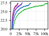
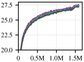
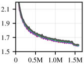
Val. BLEU		Val. BLEU		Training loss		Learning rate ${\eta_{t}}$
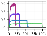
	Iteration $t$		$S$-invariant iteration $\tau_{t}$		$S$-invariant iteration $\tau_{t}$		Iteration $t$
$\mathtt{yolo}$
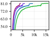
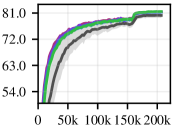
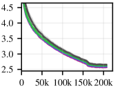
Val. mAP (%)		Val. mAP (%)		Training loss		Learning rate ${\eta_{t}}$
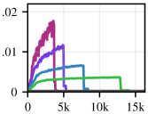
	Iteration $t$		$S$-invariant iteration $\tau_{t}$		$S$-invariant iteration $\tau_{t}$		Iteration $t$

Figure 3: AdaScale training curves. For many scales and benchmarks, AdaScale trains quality models. Training curves align closely in terms of $\tau_{t}$. In all cases, ${\eta_{t}}$ warms up gradually at the start of training, even though all $\mathtt{lr}$ schedules are simple exponential or step decay functions (which are non-increasing in $t$).

4 Empirical evaluation

We evaluate AdaScale on five practical training benchmarks. We consider a variety of tasks, models (He et al., 2016a, b; Amodei et al., 2016; Vaswani et al., 2017; Redmon & Farhadi, 2018), and datasets (Deng et al., 2009; Krizhevsky, 2009; Everingham et al., 2010; Panayotov et al., 2015). Table 1 summarizes these training benchmarks. We provide additional implementation details in Appendix B.

For each benchmark, we use one simple learning rate schedule. Specifically, $\mathtt{lr}$ is an exponential decay function for $\mathtt{cifar10}$ and $\mathtt{speech}$, and a step decay function otherwise. We use standard $\mathtt{lr}$ parameters for $\mathtt{imagenet}$ and $\mathtt{yolo}$. Otherwise, we use tuned parameters that approximately maximize the validation metric (to our knowledge, there are no standard schedules for solving $\mathtt{speech}$ and $\mathtt{transformer}$ with momentum-SGD). We use momentum $\rho=0.9$ except for $\mathtt{transformer}$, in which case we use $\rho=0.99$ for greater training stability.

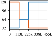
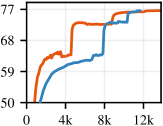
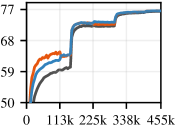
Scale $S$		Val. Acc (%)		Val. Acc (%)		Training loss
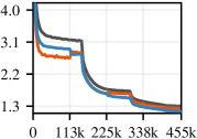
	$S$-invariant iteration $\tau_{t}$		Iteration $t$		$S$-invariant iteration $\tau_{t}$		$S$-invariant iteration $\tau_{t}$

Figure 4: Elastic AdaScaling. For $\mathtt{imagenet}$, AdaScale scales training successfully even with abrupt changes to $S$ (at $\tau_{t}=$ 133k, 225k). Unlike AdaScale, LSW degrades model quality in this setting (see Table 2).

Table 2: Comparison of final model quality. Shorthand: AS=AdaScale, LSW=Linear scaling with warm-up, LSW+=Linear scaling with warm-up and additional steps, gray=model quality significantly worse than for $S=1$ (5 trials, 0.95 significance), N/A=training diverges, Elastic$\uparrow$/$\downarrow$=elastic scaling with increasing/decreasing scale (see Figure 4). Linear scaling leads to poor model quality as the scale increases; AdaScale preserves model performance for nearly all cases.

Task	$S$	Total batch size	Validation metric			Training loss			Total iterations
			AS	LSW	LSW+	AS	LSW	LSW+	AS	LSW	LSW+
$\mathtt{cifar10}$	1	128	94.1	94.1	94.1	0.157	0.157	0.157	39.1k	39.1k	39.1k
	8	1.02k	94.1	94.0	94.0	0.153	0.161	0.145	5.85k	4.88k	5.85k
	16	2.05k	94.1	93.6	94.1	0.150	0.163	0.136	3.36k	2.44k	3.36k
	32	4.10k	94.1	92.8	94.0	0.145	0.177	0.128	2.08k	1.22k	2.08k
	64	8.19k	93.9	76.6	93.0	0.140	0.272	0.140	1.41k	611	1.41k
$\mathtt{imagenet}$	1	256	76.4	76.4	76.4	1.30	1.30	1.30	451k	451k	451k
	16	4.10k	76.5	76.3	76.5	1.26	1.31	1.27	33.2k	28.2k	33.2k
	32	8.19k	76.6	76.1	76.4	1.23	1.33	1.24	18.7k	14.1k	18.7k
	64	16.4k	76.5	75.6	76.5	1.19	1.35	1.20	11.2k	7.04k	11.2k
	128	32.8k	76.5	73.3	75.5	1.14	1.51	1.14	7.29k	3.52k	7.29k
	Elastic$\uparrow$	various	76.6	75.7	–	1.15	1.37	–	11.6k	7.04k	–
	Elastic$\downarrow$	various	76.6	74.1	–	1.23	1.45	–	13.6k	9.68k	–
$\mathtt{speech}$	1	32	79.6	79.6	79.6	2.03	2.03	2.03	84.8k	84.8k	84.8k
	4	128	81.0	80.9	81.0	5.21	4.66	4.22	22.5k	21.2k	22.5k
	8	256	80.7	80.2	80.7	6.74	6.81	6.61	12.1k	10.6k	12.1k
	16	512	80.6	N/A	N/A	7.33	N/A	N/A	6.95k	5.30k	6.95k
	32	1.02k	80.3	N/A	N/A	8.43	N/A	N/A	4.29k	2.65k	4.29k
$\mathtt{transformer}$	1	2.05k	27.2	27.2	27.2	1.60	1.60	1.60	1.55M	1.55M	1.55M
	16	32.8k	27.4	27.3	27.4	1.60	1.60	1.59	108k	99.0k	108k
	32	65.5k	27.3	27.0	27.3	1.59	1.61	1.59	58.9k	49.5k	58.9k
	64	131k	27.6	26.7	27.1	1.59	1.63	1.60	33.9k	24.8k	33.9k
	128	262k	27.4	N/A	N/A	1.59	N/A	N/A	21.4k	12.1k	21.4k
$\mathtt{yolo}$	1	16	80.2	80.2	80.2	2.65	2.65	2.65	207k	207k	207k
	16	256	81.5	81.4	81.9	2.63	2.66	2.47	15.9k	12.9k	15.9k
	32	512	81.3	80.5	81.7	2.61	2.81	2.42	9.27k	6.47k	9.27k
	64	1.02k	81.3	70.1	80.6	2.60	4.02	2.51	5.75k	3.23k	5.75k
	128	2.05k	81.4	N/A	N/A	2.57	N/A	N/A	4.07k	1.62k	4.07k

Figure 3 (and Figure 1) contains AdaScale training curves for the benchmarks and many scales. Each curve plots the mean of five distributed training runs with varying random seeds. As $S$ increases, AdaScale trains for fewer iterations and consistently preserves model quality. Interestingly, the training curves align closely when plotted in terms of scale-invariant iterations.

For $S>1$, AdaScale’s learning rate increases gradually during initial training, despite the fact that $\mathtt{lr}$ is non-increasing. Unlike warm-up, this behavior emerges naturally from a principled algorithm, not hand-tuned user input. Thus, AdaScale provides not only a compelling alternative to warm-up but also a plausible explanation for warm-up’s success.

For $\mathtt{imagenet}$, we also consider elastic scaling. Here, the only change to AdaScale is that $S$ changes abruptly after some iterations. We consider two cases: (i) $S$ increases from 32 to 64 at $\tau_{t}=T_{\mathrm{SI}}/4$ and from 64 to 128 at $\tau_{t}=T_{\mathrm{SI}}/2$, and (ii) the scale decreases at the same points, from 128 to 64 to 32. In Figure 4, we include training curves from this setting. Despite the abrupt batch size changes, AdaScale trains quality models, highlighting AdaScale’s value for the common scenario of dynamic resource availability.

As a baseline for all benchmarks, we also evaluate linear scaling with warm-up (LSW). As inputs, LSW takes single-batch schedule $\mathtt{lr}_{1}=\mathtt{lr}$ and duration $T_{1}=T_{\mathrm{SI}}$, where $\mathtt{lr}$ and $T_{\mathrm{SI}}$ are the inputs to AdaScale. Our warm-up implementation closely follows that of Goyal et al. (2017). LSW trains for $\lceil T_{1}/S\rceil$ iterations, applying warm-up to the first 5.5% of iterations. During warm-up, the learning rate increases linearly from $\mathtt{lr}_{1}(0)$ to $S\cdot\mathtt{lr}_{1}(0)$.

Since LSW trains for fewer iterations than AdaScale, we also consider a stronger baseline, LSW+, which matches AdaScale in total iterations. LSW+ uses the same learning rate schedule as LSW except scaled (stretched) along the iterations axis by the difference in training duration. We note LSW+ is significantly less practical than LSW and AdaScale, since it requires either (i) first running AdaScale to determine the number of iterations, or (ii) tuning the number of iterations.

Table 2 compares results for AdaScale, LSW, and LSW+. LSW consistently trains for fewer iterations, but doing so comes at a cost. As $S$ grows larger, LSW consistently degrades model quality and sometimes diverges. For these divergent cases, we also tested doubling the warm-up duration to 11% of iterations, and training still diverged. Similarly, even with the benefit of additional iterations, LSW+ also produces worse model quality in many cases. In contrast, AdaScale preserves model quality for nearly all cases.

		Single batch	AdaScale	LSW	Scaled SGD
		$S$$=$1, $T$$=$39.1k	$S$$=$16, $T_{\mathrm{SI}}$$=$39.1k	$S$$=$16, $T_{S1}$$=$39.1k	$S$$=$16, $T$$=$3.28k
Total $\mathtt{lr}$	decrease
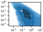
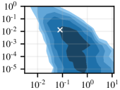
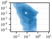
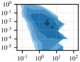
		Initial $\mathtt{lr}$	Initial $\mathtt{lr}$	Initial $\mathtt{lr}$	Initial $\mathtt{lr}$

Figure 5: AdaScale results for many learning rate schedules. Heat maps cover the space of exponential decay $\mathtt{lr}$ schedules for $\mathtt{cifar10}$. At scale 16, validation accuracies for AdaScale align closely with results for single-batch training, with the space of 94+% schedules growing moderately with AdaScale. With LSW, no schedule achieves 94% accuracy. On the right, direct $\mathtt{lr}$ search at scale 16 produces inferior results to AdaScale (here the total iterations, 3.28k, is the average total iterations among 94+% AdaScale trials). Thus, AdaScale induces a superior family of schedules for large-batch training. The white ‘$\times$’ indicates the $\mathtt{lr}$ used for Figure 1.

As a final comparison, Figure 5 demonstrates AdaScale’s performance on $\mathtt{cifar10}$ with many different $\mathtt{lr}$ schedules. We consider a 13$\times$13 grid of exponential decay schedules and plot contours of the resulting validation accuracies. At scale 16, AdaScale results align with results for single-batch training, illustrating that AdaScale preserves model quality for many schedules. Moreover, AdaScale convincingly outperforms direct search over exponential decay schedules for scaled SGD at $S$$=$16. This suggests that AdaScale provides a better learning rate family for distributed training.

5 Relation to prior work

While linear scaling with warm-up is perhaps the most popular fixed scaling rule, researchers have considered a few alternative strategies. “Square root learning rate scaling” (Krizhevsky, 2014; Li et al., 2014; Hoffer et al., 2017; You et al., 2018) multiplies learning rates by the square root of the batch size increase. Across scales, this preserves the covariance of the SGD update. Establishing this invariant remains poorly justified, however, and often root scaling degrades model quality in practice (Goyal et al., 2017; Golmant et al., 2018; Jastrzębski et al., 2018). AdaScale adapts learning rates by making ${\eta_{t}}\mathbb{E}\left[\|\bar{\mathbf{g}}_{t}\|^{2}\right]$ invariant across scales, which results in our bound from §3.3. Shallue et al. (2019) compute near-optimal parameters for many tasks and scales, and the results do not align with any fixed rule. To ensure effective training, the authors recommend avoiding such rules and re-tuning parameters for each new scale. This solution is inconvenient and resource-intensive, however, and Shallue et al. do not consider adapting learning rates to the state of training.

Many prior works have also considered the role of gradient variance in SGD. Yin et al. (2018) provide conditions—including sufficiently small batch size and sufficiently large gradient variance—under which linear learning rate scaling works well. Yin et al. do not provide an alternative strategy for adapting learning rates when linear scaling fails. McCandlish et al. (2018) study the impact of gradient variance on scaling efficiency. By averaging the relative gradient variance over the course of training, they make rough (yet fairly accurate) estimates of training time complexities as a function of scale. While McCandlish et al. (2018) do not provide an algorithm for obtaining such speed-ups, these general findings also relate to AdaScale, since gradient variance similarly determines AdaScale’s efficiency. Much like AdaScale, Johnson & Guestrin (2018) also adapt learning rates to lower amounts of gradient variance—in this case when using SGD with importance sampling. Because the variance reduction is relatively small in this setting, however, distributed training can have far greater impact on training times. Lastly, many algorithms also adapt to gradient moments for improved training, given a single batch size—see (Schaul et al., 2013; Kingma & Ba, 2015; Balles & Hennig, 2018), just to name a few. In contrast, AdaScale translates learning rates for one batch size into learning rates for a larger scale. Perhaps future versions of AdaScale will combine approaches and achieve both goals. You et al. (2017, 2020) scaled training to large batch sizes by combining adaptive gradient algorithms with scaling rule heuristics.

6 Discussion

SGD is not perfectly parallelizable. Unsurprisingly, the linear scaling rule can fail at large scales. In contrast, AdaScale accepts sublinear speedups in order to better preserve model quality. What do the speed-ups from AdaScale tell us about the scaling efficiency of SGD in general? For many problems, such as $\mathtt{imagenet}$ with batch size 32.8k, AdaScale provides lower bounds on SGD’s scaling efficiency. An important remaining question is whether AdaScale is close to optimally efficient, or if other practical algorithms can achieve similar model quality with fewer iterations.

AdaScale establishes a useful new parameterization of learning rate schedules for large-batch SGD. Practitioners can provide a simple $\mathtt{lr}$ schedule, which AdaScale adapts to learning rates for scaled training. From this, warm-up behavior emerges naturally, which produces quality models for many problems and scales. Even in elastic scaling settings, AdaScale adapts successfully to the state of training. Given these appealing qualities, it seems important to further study this family of learning rate schedules.

Based on our empirical results, as well as the algorithm’s practicality and theoretical justification, we believe AdaScale can be very valuable for distributed training.

Appendix A Proofs

In this appendix, we prove the results from §3.3 and §3. We first prove a lemma in §A.1, which we apply in the proofs. We prove Theorem 1 in §A.2, Theorem 2 in §A.3, and Theorem 3 in §A.4. We also prove Proposition 1 in §A.5 and Proposition 2 in §A.6.

A.1 Key lemma

Lemma 1.

Given Assumptions 1, 2, 3 and $\eta\in(0,2\beta^{-1})$, define $\gamma=\eta\alpha(2-\eta\beta)$ and $\Delta=\tfrac{1}{2\gamma}\eta^{2}\beta V$. Consider Algorithm 2 with $\mathtt{lr}\textrm{(}t\textrm{)}=\eta$. For all iterations $t$, we have

$$\mathbb{E}\left[F(\mathbf{w}_{t})-F^{*}\right]\leq\left[F(\mathbf{w}_{0})-F^{*}\right]\textstyle\prod_{t^{\prime}=0}^{t-1}(1-r_{t^{\prime}}\gamma)+\Delta\,.$$

Proof.

We prove this by induction. To simplify notation, let us define $\tilde{F}(\mathbf{w})=F(\mathbf{w})-F^{*}$. For $t=0$, we have

$$\mathbb{E}[\tilde{F}(\mathbf{w}_{0})]=\tilde{F}(\mathbf{w}_{0})\leq\tilde{F}(\mathbf{w}_{0})\textstyle\prod_{t^{\prime}=0}^{-1}(1-r_{t^{\prime}}\gamma)+\Delta\,.$$

Here we are using the convention $\prod_{i=0}^{-1}x_{i}=1$. For $t\geq 1$, assume the inductive hypothesis

$$\mathbb{E}[\tilde{F}(\mathbf{w}_{t-1})]\leq\tilde{F}(\mathbf{w}_{0})\prod_{t^{\prime}=0}^{t-2}(1-r_{t^{\prime}}\gamma)+\Delta\,.$$ (4)

Applying Assumption 2 (smoothness) and the update equation $\mathbf{w}_{t}=\mathbf{w}_{t-1}-r_{t-1}\eta\bar{\mathbf{g}}_{t-1}$, we have

$$\tilde{F}(\mathbf{w}_{t}) \leq\tilde{F}(\mathbf{w}_{t-1})+\langle\nabla F(\mathbf{w}_{t-1}),\mathbf{w}_{t}-\mathbf{w}_{t-1}\rangle+\tfrac{\beta}{2}\left\|\mathbf{w}_{t}-\mathbf{w}_{t-1}\right\|^{2}$$

$$=\tilde{F}(\mathbf{w}_{t-1})-r_{t-1}\eta\langle\nabla F(\mathbf{w}_{t-1}),\bar{\mathbf{g}}_{t-1}\rangle+r_{t-1}^{2}\eta^{2}\tfrac{\beta}{2}\left\|\bar{\mathbf{g}}_{t-1}\right\|^{2}\,.$$

Taking the expectation with respect to the $S$ random batches from step $t$, we have

$$\mathbb{E}\left[\tilde{F}(\mathbf{w}_{t})\mid\mathbf{w}_{t-1}\right]\leq\tilde{F}(\mathbf{w}_{t-1})-r_{t-1}\eta\left\|\nabla F(\mathbf{w}_{t-1})\right\|^{2}+r_{t-1}^{2}\eta^{2}\tfrac{\beta}{2}\mathbb{E}\left[\left\|\bar{\mathbf{g}}_{t-1}\right\|^{2}\mid\mathbf{w}_{t-1}\right]\,.$$

Now taking the expectation with respect to the distribution of $\mathbf{w}_{t-1}$, it follows that

$$\mathbb{E}\left[\tilde{F}(\mathbf{w}_{t})\right]\leq\mathbb{E}\left[\tilde{F}(\mathbf{w}_{t-1})\right]-r_{t-1}\eta\mathbb{E}\left[\left\|\nabla F(\mathbf{w}_{t-1})\right\|^{2}\right]+r_{t-1}^{2}\eta^{2}\tfrac{\beta}{2}\mathbb{E}\left[\left\|\bar{\mathbf{g}}_{t-1}\right\|^{2}\right]\,.$$ (5)

For the last term, we have

$$\mathbb{E}\left[\left\|\bar{\mathbf{g}}_{t-1}\right\|^{2}\right] =\mathbb{E}\left[\left\|(\bar{\mathbf{g}}_{t-1}-\nabla F(\mathbf{w}_{t-1}))+\nabla F(\mathbf{w}_{t-1})\right\|^{2}\right]$$

$$=\mathbb{E}\left[\left\|\bar{\mathbf{g}}_{t-1}-\nabla F(\mathbf{w}_{t-1})\right\|^{2}+\left\|\nabla F(\mathbf{w}_{t-1})\right\|^{2}\right]$$

$$=\mathbb{E}\left[\tfrac{1}{S}\sigma_{\mathbf{g}}^{2}(\mathbf{w}_{t-1})+\left\|\nabla F(\mathbf{w}_{t-1})\right\|^{2}\right]$$

$$=\frac{1}{r_{t-1}}\mathbb{E}\left[\sigma_{\mathbf{g}}^{2}(\mathbf{w}_{t-1})+\left\|\nabla F(\mathbf{w}_{t-1})\right\|^{2}\right]$$

$$\leq\frac{1}{r_{t-1}}\left(\mathbb{E}\left[\left\|\nabla F(\mathbf{w}_{t-1})\right\|^{2}\right]+V\right)\,.$$ (6)

Combining (6) with (5), we have

$$\mathbb{E}\left[\tilde{F}(\mathbf{w}_{t})\right] \leq\mathbb{E}\left[\tilde{F}(\mathbf{w}_{t-1})\right]-r_{t-1}\eta(1-\eta\tfrac{\beta}{2})\mathbb{E}\left[\left\|\nabla F(\mathbf{w}_{t-1})\right\|^{2}\right]+r_{t-1}\eta^{2}\tfrac{\beta}{2}V$$

$$\leq(1-r_{t-1}\gamma)\mathbb{E}\left[\tilde{F}(\mathbf{w}_{t-1})\right]+r_{t-1}\gamma\Delta\,.$$ (7)

In this last step, we applied Assumption 1 (PL condition) and plugged in definitions for $\gamma$ and $\Delta$.

To complete the proof, we apply (4):

$$\mathbb{E}[\tilde{F}(\mathbf{w}_{t})] \leq(1-r_{t-1}\gamma)\left(\tilde{F}(\mathbf{w}_{0})\prod_{t^{\prime}=0}^{t-2}(1-r_{t^{\prime}}\gamma)+\Delta\right)+r_{t-1}\gamma\Delta$$

$$=\tilde{F}(\mathbf{w}_{0})\prod_{t^{\prime}=0}^{t-1}(1-r_{t^{\prime}}\gamma)+\Delta\,.$$

∎

A.2 Proof of Theorem 1

See 1

Proof.

The theorem is a special case of Lemma 1. In particular, Algorithm 1 with inputs $\mathtt{lr}\textrm{(}t\textrm{)}=\eta$, $S=1$, and $T$ iterations is equivalent to Algorithm 2 with $T_{\mathrm{SI}}=T$ and the same scale and learning rate inputs. This follows from the fact that $r_{t}=1$ for all iterations of AdaScale when $S=1$. Thus, we can obtain the result by plugging $t=T$ into the bound from Lemma 1. ∎

A.3 Proof of Theorem 2

See 2

Proof.

Let $T$ denote the total iterations for Algorithm 2. Applying Lemma 1, we have

$$\mathbb{E}\left[F(\mathbf{w}_{t})-F^{*}\right]\leq(F(\mathbf{w}_{0})-F^{*})\prod_{t^{\prime}=0}^{T-1}(1-r_{t^{\prime}}\gamma)+\Delta\,.$$ (8)

Now note that for any $r\geq 1$ and $x\in[0,1]$, we have

$$1-rx\leq(1-x)^{r}.$$ (9)

This holds because for any $r\geq 1$ and $x\in[0,1]$, the function $(1-x)^{r}$ is convex in $x$, and $1-rx$ is tangent to this function at $x=0$. Thus,

$$\prod_{t^{\prime}=0}^{T-1}(1-r_{t^{\prime}}\gamma)\leq(1-\gamma)^{\sum_{t^{\prime}=0}^{T-1}r_{t^{\prime}}}\,.$$ (10)

Note that this requires $1-r_{t}\gamma\geq 0$ for all $t$, which is true because $r_{t}\leq S\leq\gamma^{-1}$. Now plugging (10) into (8),

$$\mathbb{E}\left[F(\mathbf{w}_{t})-F^{*}\right] \leq(F(\mathbf{w}_{0})-F^{*})(1-\gamma)^{\sum_{t^{\prime}=0}^{T-1}r_{t^{\prime}}}+\Delta$$

$$=(F(\mathbf{w}_{0})-F^{*})(1-\gamma)^{\bar{r}T}+\Delta\,.$$

∎

A.4 Proof of Theorem 3

See 3

Proof.

We reduce the theorem to a special case of Theorem 1. Define $\tilde{\mathbf{x}}=(\tilde{\mathbf{x}}^{(1)},\ldots,\tilde{\mathbf{x}}^{(S)})$, where $\tilde{\mathbf{x}}^{(i)}\sim\mathcal{X}$ for each $i\in[S]$, and $\tilde{\mathbf{x}}^{(1)},\ldots,\tilde{\mathbf{x}}^{(S)}$ are jointly independent. Denote by $\tilde{\mathcal{X}}$ the distribution of $\tilde{\mathbf{x}}$. Also define

$$\tilde{f}(\mathbf{w},\tilde{\mathbf{x}})=\frac{1}{S}\sum_{i=1}^{S}f(\mathbf{w},\tilde{\mathbf{x}}^{(i)})\,.$$

It follows that for any $\mathbf{w}$,

$$\mathbb{E}_{\tilde{\mathbf{x}}}\left[\|\nabla\tilde{f}(\mathbf{w},\tilde{\mathbf{x}})-\nabla F(\mathbf{w})\|^{2}\right]=\frac{1}{S}\sigma_{\mathbf{g}}^{2}(\mathbf{w})\leq\frac{V}{S}\,.$$

The algorithm described in Theorem 3 is identical to running Algorithm 1 with scale $1$, batch distribution $\tilde{\mathcal{X}}$, loss $\tilde{f}$, learning rate $\mathtt{lr}\textrm{(}t\textrm{)}=S\eta$, and variance upper bound $\frac{V}{S}$. Plugging these values into Theorem 1, we have

$$\mathbb{E}\left[F(\mathbf{w}_{T})-F^{*}\right] \leq(1-S\eta\alpha(2-S\eta\beta))^{T}[F(\mathbf{w}_{0})-F^{*}]+\frac{S\eta\beta VS^{-1}}{2\alpha\left(2-S\eta\beta\right)}$$

$$=\left(1-S\gamma\cdot\left(\tfrac{2-S\eta\beta}{2-\eta\beta}\right)\right)^{T}[F(\mathbf{w}_{0})-F^{*}]+\left(\tfrac{2-\eta\beta}{2-S\eta\beta}\right)\Delta$$

$$\leq\left(1-\gamma\cdot\left(\tfrac{2-S\eta\beta}{2-\eta\beta}\right)\right)^{ST}[F(\mathbf{w}_{0})-F^{*}]+\left(\tfrac{2-\eta\beta}{2-S\eta\beta}\right)\Delta\,.$$

The last step follows from (9). ∎

A.5 Proof of Proposition 1

See 1

Proof.

Since the gradient variance is zero, the $\mathtt{compute\_gradient}$ function returns $\nabla F(\mathbf{w}_{t})$, which does not depend on $S$. Thus, $\mathbf{w}^{(S)}=\mathbf{w}^{(1)}$ and $F(\mathbf{w}^{(S)})=F(\mathbf{w}^{(1)})$. ∎

A.6 Proof of Proposition 2

See 2

Proof.

The scaled SGD algorithm runs for ${\nu T}/S$ iterations and follows the update rule

$$\mathbf{w}_{t+1}=\mathbf{w}_{t}-\tfrac{S{\eta}}{\nu}\nabla F(\mathbf{w}_{t})+\tfrac{S{\eta}}{\nu}\bm{\xi}_{t}\,.$$

Here $\bm{\xi}_{t}$ is normally distributed with $\mathbb{E}\left[\bm{\xi}_{t}\right]=\mathbf{0}$ and $\mathrm{cov}(\bm{\xi}_{t},\bm{\xi}_{t})=\tfrac{\nu}{S}\bm{\Sigma}$. In the limit $\nu\rightarrow+\infty$, this difference equation converges to a stochastic differential equation on the interval $[0,{\eta}{T}]$ (Kloeden & Platen, 1992, Chapter 9):

$$d\mathbf{w}=-\nabla F(\mathbf{w})dt+({\eta}\bm{\Sigma})^{1/2}d\mathbf{W}(t)\,,\quad\text{where}\quad\mathbf{W}(t)\sim\mathcal{N}(\mathbf{0},\mathbf{I})\,.$$

Since this SDE does not depend on $S$, the distributions of $\mathbf{w}^{(S)}$ and $\mathbf{w}^{(1)}$ are identical in this limit. Thus, we have $\mathbb{E}[F(\mathbf{w}^{(S)})]=\mathbb{E}[F(\mathbf{w}^{(1)})]$. ∎

Appendix B Additional details on empirical comparisons

This appendix provides additional details of our experiment set-up.

B.1 Learning rate schedules

We describe the $\mathtt{lr}$ schedules for each training benchmark in Table 3. We use two learning rate families: exponential decay and step decay. Using parameters $\eta_{0}$, $d$, and $w_{i}$, we define $\mathtt{lr}\textrm{(}t\textrm{)}=\eta_{0}d^{(t/T_{S1})}$ for exponential decay families and $\mathtt{lr}\textrm{(}t\textrm{)}=\eta_{0}d^{\sum_{i}^{n}\mathbbm{1}[{t>w_{i}}]}$ for step decay families. Here $T_{S1}$ denotes the total iterations for scale $S=1$. Note that in all cases, we use simple schedules and no warm-up.

Table 3: Learning rate schedules for training benchmarks.

Benchmark	Learning rate famliy	$\eta_{0}$	$d$	$w_{i}$
$\mathtt{cifar10}$	Exponential decay	0.08	0.0133	N/A
$\mathtt{imagenet}$	Step decay	0.1	0.1	150,240, 300,480, 400,640
$\mathtt{speech}$	Exponential decay	1.4 $\times 10^{-3}$	0.05	N/A
$\mathtt{transformer}$	Step decay	0.01	0.1	1,440,000
$\mathtt{yolo}$	Step decay	2.5 $\times 10^{-4}$	0.1	160,000, 180,000

For $\mathtt{imagenet}$ and $\mathtt{yolo}$, we used standard learning rate schedules from (Goyal et al., 2017) and (Zhang et al., 2019). For $\mathtt{cifar10}$, $\mathtt{speech}$, and $\mathtt{transformer}$, we chose learning rate parameters, via hand-tuning, that approximately maximized model quality. This was necessary for $\mathtt{speech}$ and $\mathtt{transformer}$, since our reference implementations train with the Adam optimizer (Kingma & Ba, 2015), and momentum-SGD requires different learning rate values.

B.2 Warm-up implementation

Our warm-up procedure closely follows the strategy of Goyal et al. (2017). We apply warm-up for the first 5.5% of training iterations—we denote this number by $W_{S}$. During warm-up, the learning rate increases linearly, starting at the initial learning rate for single-batch training and finishing at $S$ times this value. After warm-up, we apply linear scaling to the single-batch schedule. Following Goyal et al. (2017), we modify this scaled schedule so that the total iterations, including warm-up, is proportional to $S^{-1}$. For step-decay schedules, we omit the first $W_{S}$ iterations after warm-up. For exponential decay schedules, we compress the scaled schedule by $W_{S}$ iterations, using slightly faster decay.

B.3 Numerical stability strategy for AdaScale implementation

As discussed in §3.4, the AdaScale implementation for our empirical results uses an alternative strategy for ensuring numerical stability instead of the recommendation from §3.4. The recommended strategy is simpler, but the results should not differ significantly.

For the experiments, we estimate mean and variance quantities separately. Algebraically, this gain estimator is equivalent to that of §3.4, except for the numerical stability measures. In particular, we define

$$\begin{array}[]{c}\\[-13.50008pt] \textstyle\hat{\sigma}^{2}_{t}=\tfrac{1}{S-1}\sum_{i=1}^{S}\|\mathbf{g}_{t}^{(i)}\|^{2}-\tfrac{S}{S-1}\left\|\bar{\mathbf{g}}_{t}\right\|^{2}\,,\\ \\[-8.99994pt] \text{and}\quad\hat{\mu}^{2}_{t}=\left\|\bar{\mathbf{g}}_{t}\right\|^{2}-\tfrac{1}{S}\hat{\sigma}^{2}_{t}\,.\\ \\[-13.99995pt] \end{array}$$

Here $\hat{\sigma}^{2}_{t}$ and $\hat{\mu}^{2}_{t}$ are unbiased estimates of $\mathbb{E}_{\mathbf{w}_{t}}[\sigma_{\mathbf{g}}^{2}(\mathbf{w}_{t})]$ and $\mathbb{E}_{\mathbf{w}_{t}}[\mu_{\mathbf{g}}^{2}(\mathbf{w}_{t})]$. We estimate $r_{t}$ by plugging in moving averages $\bar{\sigma}^{2}_{t}$ and $\bar{\mu}_{t}^{2}$, which average $\hat{\sigma}^{2}_{t}$ and $\hat{\mu}^{2}_{t}$ over prior iterations. The implementation uses exponential moving average parameter $\theta=\max\{1-S/1000,0\}$, where $\theta=0$ results in no averaging. Before averaging, we set $\hat{\sigma}^{2}_{t}\leftarrow\mathrm{max}(\hat{\sigma}^{2}_{t},\epsilon)$ (to prevent division by zero) and $\hat{\mu}^{2}_{t}\leftarrow\mathrm{max}(\hat{\mu}^{2}_{t},0)$ (to ensure $r_{t}\in[1,S]$). To initialize, we set $r_{0}\leftarrow 1$, and for iterations $t<(1-\theta)^{-1}$, we define $\bar{\sigma}^{2}_{t}$ and $\bar{\mu}_{t}^{2}$ as the mean of past samples. The averaging procedure does not factor $\hat{\sigma}^{2}_{t}$ and $\hat{\mu}^{2}_{t}$ into the estimate for $r_{t}$ (only mean and variance estimates from prior iterations), but we recommend using estimates from the current iteration if possible.

B.4 Benchmark-specific implementation details

Here we describe implementation details that are specific to each benchmark task.

B.4.1 $\mathtt{cifar10}$

We train ResNet-18 (preactivation) models (He et al., 2016b), using the standard training data split for CIFAR-10 (Krizhevsky, 2009). We use weight decay $=5\times 10^{-4}$. For batch normalization, we use parameters momentum $=0.995$ and $\epsilon=2\times 10^{-5}$, and we do not train the batch normalization scaling parameters. We apply standard data augmentation during training. Specifically, we pad images to $40\times 40$ and random crop to $32\times 32$, and we also apply random horizontal reflections.

B.4.2 $\mathtt{imagenet}$

For ImageNet classification (Deng et al., 2009), we train ResNet-50 models (He et al., 2016a). Our implementation closely follows the implementation of Goyal et al. (2017). We use stride-2 convolutions on $3\times 3$ layers. For each block’s final batch normalization layer, we initialize the batch norm scaling parameters to $0$ (and we initialize to $1$ everywhere else). We use weight decay parameter $10^{-4}$. Since each GPU processes 128 examples per batch, we use ghost batch normalization (Hoffer et al., 2017) with ghost batch size $32$. We resize input images to $224\times 224\times 3$. For data augmentation, we apply random cropping and left-right mirroring during training.

B.4.3 $\mathtt{speech}$

We use Amodei et al. (2016)’s Deep Speech 2 model architecture. The model consists of two 2D convolutional input layers, five bidirectional RNN layers, one fully connected layer, and softmax outputs. Each convolutional layer has $32$ filters. The RNN layers use GRU cells with hidden size $800$. We apply batch normalization to the inputs of each layer. The batch norm parameters are momentum $=0.997$ and $\epsilon=10^{-5}$. The loss is CTC loss. We apply gradient clipping with threshold $100$. The inputs to the network are log spectrograms, which we compute using $20$ms windows from audio waveforms sampled at $16$ kHz. The training data is the train-clean-100 and train-clean-360 partitions of the OpenSLR LibriSpeech Corpus, which amounts to 460 hours of recorded speech. We evaluate models on the dev-clean partition and use the CTC greedy decoder for decoding.

B.4.4 $\mathtt{transformer}$

We train Transformer base models (Vaswani et al., 2017). We use dynamic batching with at most $256$ tokens per example. In Table 2, the “batch size” is the maximum number of tokens processed per iteration. Our implementation closely follows that of Vaswani et al. (2017). Unlike Vaswani et al., we use only the final model for evaluation instead of the average of the last five checkpoints. We train on the WMT 2014 English-German dataset and evaluate on the newstest2014 test set. We compute BLEU scores using the script in the official TensorFlow GitHub repository, https://github.com/tensorflow/models/blob/master/official/transformer/compute_bleu.py

B.4.5 $\mathtt{yolo}$

We train YOLOv3 models (Redmon & Farhadi, 2018). To achieve high mAP scores, we also apply mixup (Zhang et al., 2018) and class label smoothing, following (Zhang et al., 2019). We also use focal loss. We use batch normalization momentum$=0.9$ and weight decay $=5\times 10^{-4}$. We resize input images to $416\times 416$ (for both training and validation). We report mAP values at IOU threshold $0.5$. We use the Pascal VOC 2007 trainval and 2012 trainval datasets for training and the 2007 test set for validation (Everingham et al., 2010). During training, we initialize the darknet-53 convolutional layers with weights trained on ImageNet.

B.5 Miscellaneous

In practice, wall time speed-ups also depend on system scaling efficiency. Since most aspects of system scaling relate orthogonally to the training algorithm, we limit our scope to algorithmic aspects of training.

For Figure 5, one dimension defines initial value $\mathtt{lr}\textrm{(}0\textrm{)}$, and the second dimension specifies total decrease $\mathtt{lr}\textrm{(}T_{\mathrm{SI}}\textrm{)}/\mathtt{lr}\textrm{(}0\textrm{)}$. For single-batch training, we use $T=39.1\times 10^{3}$ steps. We run AdaScale and the LW baseline at $S=16$, and we compare the final validation accuracies.

Appendix C Robustness to averaging parameter

In this appendix, we test the robustness of AdaScale to the averaging parameter $\theta$ for estimating gain ratios (see §3.4). When $\theta=0$, AdaScale does not average estimates of gradient moments. The closer $\theta$ is to $1$, the more that AdaScale averages across iterations.

Using the $\mathtt{cifar10}$ benchmark, we compare four values of $\theta$ at scales $S=8$ and $S=32$. The case $\theta=1-S/1000$ corresponds to the $\mathtt{cifar10}$ experiment for Figure 1. We average the resulting metrics over five trials. Figure 6 contains the training curves.

$S=8$
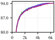
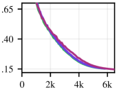
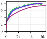
Val. Acc (%)		Train objective		Gain $r_{t}$		Learning rate ${\eta_{t}}$
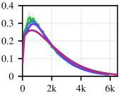
	Iteration $t$		Iteration $t$		Iteration $t$		Iteration $t$
$S=32$
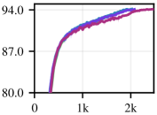
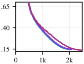
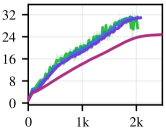
Val. Acc (%)		Train objective		Gain $r_{t}$		Learning rate ${\eta_{t}}$
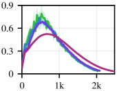
	Iteration $t$		Iteration $t$		Iteration $t$		Iteration $t$

Figure 6: AdaScale training curves with varying moving average parameter.

We also include final metric values in Table 4.

Table 4: AdaScale final metrics with varying moving average parameter.

$S$	$\theta$	Final val. accuracy (%)	Final train objective	Total iterations
8	$1-S/10$	94.0	0.153	5.75k
	$1-S/100$	94.1	0.154	5.78k
	$1-S/1000$	94.1	0.153	5.85k
	$1-S/10000$	94.1	0.147	6.45k
32	$0$	94.0	0.145	2.02k
	$1-S/100$	94.1	0.147	2.03k
	$1-S/1000$	94.1	0.145	2.08k
	$1-S/10000$	94.1	0.136	2.46k

For the three smaller settings of $\theta$, the results align very closely. This suggests that AdaScale is robust to the choice of $\theta$. When $\theta=1-S/10000$, we see that smoothing more significantly biases gain ratio estimates, which leads to more contrasting results.

Appendix D Additional empirical results

This appendix provides additional empirical results.

D.1 Gain ratio estimation

Our online gain ratio estimates align closely with offline estimates (computed by averaging over 1000 batches). Figure 7 demonstrates this for the $\mathtt{transformer}$ task.

	$\mathtt{transformer}$, $S$$=$16	$\mathtt{transformer}$, $S$$=$128
Gain ratio $r_{t}$
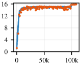
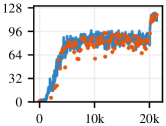
	Iteration $t$	Iteration $t$

Figure 7: Gain ratios for $\mathtt{transformer}$. Plots compare moving average $r_{t}$ estimates to values computed offline (using 1000 batches).

D.2 $\mathtt{cifar10}$ AdaScale training curves

Figure 8 shows additional plots for the $\mathtt{cifar10}$ task. Notably, the plots show training loss curves at various scales and full view of the learning rate curves.

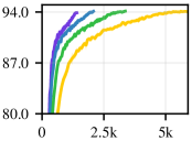
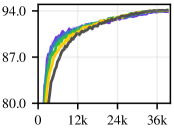
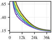
Val. Acc (%)		Val. Acc (%)		Training loss		Learning rate ${\eta_{t}}$
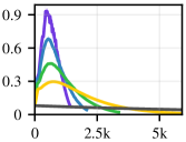
	Iteration $t$		$S$-invariant iteration $\tau_{t}$		$S$-invariant iteration $\tau_{t}$		Iteration $t$

Figure 8: AdaScale training curves for $\mathtt{cifar10}$. AdaScale trains quality models at various scales.

References

- Amodei et al. (2016) Amodei, D., Anubhai, R., Battenberg, E., Case, C., Casper, J., Catanzaro, B., Chen, J., Chrzanowski, M., Coates, A., Diamos, G., Elsen, E., Engel, J. H., Fan, L., Fougner, C., Han, T., Hannun, A. Y., Jun, B., LeGresley, P., Lin, L., Narang, S., Ng, A. Y., Ozair, S., Prenger, R., Raiman, J., Satheesh, S., Seetapun, D., Sengupta, S., Wang, Y., Wang, Z., Wang, C., Xiao, B., Yogatama, D., Zhan, J., and Zhu, Z. Deep speech 2: End-to-end speech recognition in English and Mandarin. In Proceedings of the 33rd International Conference on Machine Learning, 2016.
- Balles & Hennig (2018) Balles, L. and Hennig, P. Dissecting Adam: The sign, magnitude and variance of stochastic gradients. In Proceedings of the 35th International Conference on Machine Learning, 2018.
- Charles & Papailiopoulos (2018) Charles, Z. and Papailiopoulos, D. Stability and generalization of learning algorithms that converge to global optima. In Proceedings of the 35th International Conference on Machine Learning, 2018.
- De et al. (2017) De, S., Yadav, A., Jacobs, D., and Goldstein, T. Automated inference with adaptive batches. In Proceedings of the 20th International Conference on Artificial Intelligence and Statistics, 2017.
- Defazio et al. (2014) Defazio, A., Bach, F., and Lacoste-Julien, S. SAGA: A fast incremental gradient method with support for non-strongly convex composite objectives. In Advances in Neural Information Processing Systems 27, 2014.
- Deng et al. (2009) Deng, J., Dong, W., Socher, R., Li, L.-J., Li, K., and Fei-Fei, L. ImageNet: A Large-Scale Hierarchical Image Database. In IEEE Conference on Computer Vision and Pattern Recognition, 2009.
- Devarakonda et al. (2017) Devarakonda, A., Naumov, M., and Garland, M. AdaBatch: Adaptive batch sizes for training deep neural networks. arXiv:1712.02029, 2017.
- Everingham et al. (2010) Everingham, M., Gool, L. V., Williams, C. K. I., Winn, J., and Zisserman, A. The pascal visual object classes (VOC) challenge. International Journal of Computer Vision, 88(2):303–338, 2010.
- Ghorbani & Krishnan (2019) Ghorbani, B. and Krishnan, S. An investigation into neural net optimization via hessian eigenvalue density. arXiv:1901.10159, 2019.
- Golmant et al. (2018) Golmant, N., Vemuri, N., Yao, Z., Feinberg, V., Gholami, A., Rothauge, K., Mahoney, M. W., and Gonzalez, J. On the computational inefficiency of large batch sizes for stochastic gradient descent. arXiv:1811.12941, 2018.
- Goyal et al. (2017) Goyal, P., Dollár, P., Girshick, R., Noordhuis, P., Wesolowski, L., Kyrola, A., Tulloch, A., Jia, Y., and He, K. Accurate, large minibatch SGD: Training ImageNet in one hour. arXiv:1706.02677, 2017.
- He et al. (2016a) He, K., Zhang, X., Ren, S., and Sun, J. Deep residual learning for image recognition. In Proceedings of the IEEE conference on computer vision and pattern recognition, 2016a.
- He et al. (2016b) He, K., Zhang, X., Ren, S., and Sun, J. Identity mappings in deep residual networks. In European conference on computer vision, 2016b.
- Hoffer et al. (2017) Hoffer, E., Hubara, I., and Soudry, D. Train longer, generalize better: Closing the generalization gap in large batch training of neural networks. In Advances in Neural Information Processing Systems 30, 2017.
- Jain et al. (2018) Jain, P., Kakade, S. M., Kidambi, R., Netrapalli, P., and Sidford, A. Parallelizing stochastic gradient descent for least squares regression: Mini-batching, averaging, and model misspecification. Journal of Machince Learning Research, 18(223):1–42, 2018.
- Jastrzębski et al. (2018) Jastrzębski, S., Kenton, Z., Arpit, D., Ballas, N., Fischer, A., Bengio, Y., and Storkey, A. J. Three factors influencing minima in SGD. In Proceedings of the 27th International Conference on Artificial Neural Networks, 2018.
- Johnson & Zhang (2013) Johnson, R. and Zhang, T. Accelerating stochastic gradient descent using predictive variance reduction. In Advances in Neural Information Processing Systems 26, 2013.
- Johnson & Guestrin (2018) Johnson, T. B. and Guestrin, C. Training deep models faster with robust, approximate importance sampling. In Advances in Neural Information Processing Systems 31, 2018.
- Karimi et al. (2016) Karimi, H., Nutini, J., and Schmidt, M. Linear convergence of gradient and proximal-gradient methods under the polyak-łojasiewicz condition. In Joint European Conference on Machine Learning and Knowledge Discovery in Databases, 2016.
- Kingma & Ba (2015) Kingma, D. P. and Ba, J. Adam: A method for stochastic optimization. In Proceedings of the 3rd International Conference on Learning Representations, 2015.
- Kloeden & Platen (1992) Kloeden, P. E. and Platen, E. Numerical Solution of Stochastic Differential Equations. Springer, 1992.
- Krizhevsky (2009) Krizhevsky, A. Learning multiple layers of features from tiny images. Technical report, 2009.
- Krizhevsky (2014) Krizhevsky, A. One weird trick for parallelizing convolutional neural networks. arXiv:1404.5997, 2014.
- Lei et al. (2017) Lei, L., Ju, C., Chen, J., and Jordan, M. I. Nonconvex finite-sum optimization via SCSG methods. In Advances in Neural Information Processing Systems 30, 2017.
- Li et al. (2014) Li, M., Zhang, T., Chen, Y., and Smola, A. J. Efficient mini-batch training for stochastic optimization. In Proceedings of the 20th ACM SIGKDD Interational Conference on Knowledge Discovery and Data Mining, 2014.
- Lin et al. (2019) Lin, H., Zhang, H., Ma, Y., He, T., Zhang, Z., Zha, S., and Li, M. Dynamic mini-batch SGD for elastic distributed training: Learning in the limbo of resources. arXiv:1904.12043, 2019.
- Ma et al. (2018) Ma, S., Bassily, R., and Belkin, M. The power of interpolation: Understanding the effectiveness of SGD in modern over-parametrized learning. In Proceedings of the 35th International Conference on Machine Learning, 2018.
- McCandlish et al. (2018) McCandlish, S., Kaplan, J., Amodei, D., and Team, O. D. An empirical model of large-batch training. arXiv:1812.06162, 2018.
- Needell et al. (2014) Needell, D., Ward, R., and Srebro, N. Stochastic gradient descent, weighted sampling, and the randomized Kaczmarz algorithm. In Advances in Neural Information Processing Systems 27, 2014.
- Panayotov et al. (2015) Panayotov, V., Chen, G., Povey, D., and Khudanpur, S. Librispeech: An ASR corpus based on public domain audio books. In IEEE International Conference on Acoustics, Speech and Signal Processing, 2015.
- Reddi et al. (2016) Reddi, S. J., Hefny, A., Sra, S., Póczoós, B., and Smola, A. Stochastic variance reduction for nonconvex optimization. In Proceedings of the 33rd International Conference on Machine Learning, 2016.
- Redmon & Farhadi (2018) Redmon, J. and Farhadi, A. YOLOv3: An incremental improvement. arXiv:1804.02767, 2018.
- Sagun et al. (2017) Sagun, L., Evci, U., Guney, V. U., Dauphin, Y., and Bottou, L. Empirical analysis of the hessian of over-parametrized neural networks. arXiv:1706.04454, 2017.
- Schaul et al. (2013) Schaul, T., Zhang, S., and LeCun, Y. No more pesky learning rates. In Proceedings of the 30th International Conference on Machine Learning, 2013.
- Shallue et al. (2019) Shallue, C. J., Lee, J., Antognini, J., Sohl-Dickstein, J., Frostig, R., and Dahl, G. E. Measuring the effects of data parallelism on neural network training. Journal of Machince Learning Research, 20(112):1–49, 2019.
- Smith et al. (2018) Smith, S., Kindermans, P., Ying, C., and Le, Q. V. Don’t decay the learning rate, increase the batch size. In Proceedings of the 6th International Conference on Learning Representations, 2018.
- Sun (2019) Sun, R. Optimization for deep learning: theory and algorithms. arXiv:1912.08957, 2019.
- Vaswani et al. (2017) Vaswani, A., Shazeer, N., Parmar, N., Uszkoreit, J., Jones, L., Gomez, A. N., Kaiser, L., and Polosukhin, I. Attention is all you need. In Advances in Neural Information Processing Systems 31, 2017.
- Yin et al. (2018) Yin, D., Pananjady, A., Lam, M., Papailiopoulos, D., Ramchandran, K., and Bartlett, P. Gradient diversity: A key ingredient for scalable distributed learning. In Proceedings of the 21st International Conference on Artificial Intelligence and Statistics, 2018.
- You et al. (2017) You, Y., Gitman, I., and Ginsburg, B. Large batch training of convolutional networks. arXiv:1708.03888, 2017.
- You et al. (2018) You, Y., Hseu, J., Ying, C., Demmel, J., Keutzer, K., and Hsieh, C. Large-batch training for LSTM and beyond. In NeurIPS Workshop on Systems for ML and Open Source Software, 2018.
- You et al. (2020) You, Y., Li, J., Reddi, S., Hseu, J., Kumar, S., Bhojanapalli, S., Song, X., Demmel, J., Keutzer, K., and Hsieh, C.-J. Large batch optimization for deep learning: Training bert in 76 minutes. In International Conference on Learning Representations, 2020.
- Yuan et al. (2019) Yuan, Z., Yan, Y., Jin, R., and Yang, T. Stagewise training accelerates convergence of testing error over sgd. In Advances in Neural Information Processing Systems 32, 2019.
- Zhang et al. (2018) Zhang, H., Cisse, M., Dauphin, Y. N., and Lopez-Paz, D. Mixup: Beyond empirical risk minimization. In International Conference on Learning Representations, 2018.
- Zhang et al. (2019) Zhang, Z., He, T., Zhang, H., Zhang, Z., Xie, J., and Li, M. Bag of freebies for training object detection neural networks. arXiv:1902.04103, 2019.
- Zhao & Zhang (2015) Zhao, P. and Zhang, T. Stochastic optimization with importance sampling for regularized loss minimization. In Proceedings of the 32nd International Conference on Machine Learning, 2015.