Locating quantum critical points with Kibble-Zurek quenches

Abstract

We describe a scheme for finding quantum critical points based on studies of a non-equilibrium susceptibility during finite-rate quenches taking the system from one phase to another. We assume that two such quenches are performed in opposite directions, and argue that they lead to formation of peaks of a non-equilibrium susceptibility on opposite sides of a critical point. Its position is then narrowed to the interval marked off by these values of the parameter driving the transition, at which the peaks are observed. Universal scaling with the quench time of precision of such an estimation is derived and verified in two exactly solvable models. Experimental relevance of these results is expected.

I Introduction

Non-equilibrium phase transitions are ubiquitous in Nature. Their studies, in the context relevant for this work, were started by Kibble, who investigated cosmological phase transitions of the early Universe Kib . It was then proposed by Zurek that similar phenomena can be approached in tabletop condensed matter systems Zur . These theoretical investigations triggered experimental work on non-equilibrium dynamics of superconductors, Josephson junctions, superfluids, cold atoms and ions, liquid crystals, multiferroics, convective fluids, colloids, etc. Recent surveys of these efforts, discussing dynamics of both classical and quantum phase transitions, can be found in Kibble (2007); Jac (a); Pol (a); del (a, b).

Non-equilibrium dynamics, we are interested in, comes from finite-rate driving of a system across its critical point. Key features of this process are captured by the Kibble-Zurek (KZ) theory, which relates non-equilibrium response of a system to the quench rate and some universal critical exponents.

Phase transitions, however, are also characterized by non-universal properties, among which the position of the critical point clearly stands out. Indeed, by the very definition, it gives us the physical parameter(s) at which the properties of the system fundamentally change. Such a dramatic change is possible due to the fact that some of the most interesting many-body physics takes place near critical points, where distant parts of the system get correlated and its response to external perturbations significantly slows down. Our understanding of such phenomena builds on the insights coming from the renormalization-group theory, whose basic assumptions are best justified very close to critical points Car . Detailed studies of these and related phenomena cannot proceed without accurate determination of critical points. Their knowledge is also of practical importance, which is perhaps best seen in all devices involving superconductors.

It is the purpose of this work to discuss a propitious KZ-related scheme for localization of quantum critical points (QCPs)–see Fig. 1 for its schematic presentation. So, we will be dealing with quantum phase transitions Coleman and Schofield (2005); Sac (a); Con ; Sac (b), whose dynamical studies, in the framework of the quantum KZ theory, were initiated by BDP (a); Dor (a); Jac (b). Preceding work on quench-based localization of QCPs can be found in Yin et al. ; Hu et al. (2015); Huang and Yin (2019), where finite-rate quenches were used, and in Arn (a); Roy et al. (2017), where instantaneous ones were employed. These studies differ from our work in the strategy employed for extraction of QCPs and quench protocols that are used for such a purpose.

The outline of this paper is the following. We explain the idea behind our work in Sec. II. Calculations supporting it are presented in Secs. III and IV, where respectively extended $XY$ and Ising models are considered. Conclusions and outlook can be found in Sec. V. Technical details, pertinent to studies from Secs. III and IV, are laid out in Appendices B and A, respectively. Finally, derivation of the scaling ansatz from Sec. IV is discussed in Appendix C.

II Idea

To explain the logic behind our work, we consider some susceptibility $\chi$, whose ground-state value $\chi^{eq}$ is algebraically divergent at the QCP $g_{c}$, say

$$\chi^{eq}(g)=\chi^{eq}_{reg}(g)+\chi^{eq}_{sing}(g),$$ (1)

$$\chi^{eq}_{sing}(g)\sim|g-g_{c}|^{-\gamma},\ \gamma>0,$$

where the regular (singular) at $g_{c}$ part of $\chi^{eq}$ is denoted as $\chi^{eq}_{reg}$ ($\chi^{eq}_{sing}$).

The system will be initially prepared in a ground state far away from the QCP. It will be then quenched towards it by linear in time ramp up of the external parameter driving the transition

$$g(t)=g_{c}+\frac{t}{\tau_{Q}},$$ (2)

where inverse of the quench time $\tau_{Q}$ provides the quench rate and the QCP is reached at the time $t_{c}=0$.

As long as the system will be far away from the QCP, its evolution will be adiabatic and so its susceptibility will closely match its instantaneous equilibrium value. Near the QCP, however, the evolution cannot be adiabatic because the reaction time of the system, given by the inverse of its energy gap BDP (a), diverges at $g_{c}$. So, the susceptibility $\chi(g(t))$ should lag behind $\chi^{eq}(g(t))$. The mismatch between the two will be largest at the QCP, where $\chi(g_{c})$, unlike $\chi^{eq}(g_{c})$, will be finite (no singularities are expected in the non-equilibrium state of the system as it will not be given enough time to develop them). Another consequence of the delayed reaction to crossing of the QCP should be seen in the maximum of $\chi(g(t))$, which we expect to appear past the QCP, say at $g_{*}^{\uparrow}>g_{c}$.

Suppose now that the system is initially prepared in a ground state on the other side of the transition, and the parameter $g(t)$ is ramped down. The same discussion then leads to the conclusion that $\chi(g(t))$ should have the maximum at some $g_{*}^{\downarrow}<g_{c}$. Therefore, we expect that location of the QCP can be pinned down to the interval $(g_{*}^{\downarrow},g_{*}^{\uparrow})$.

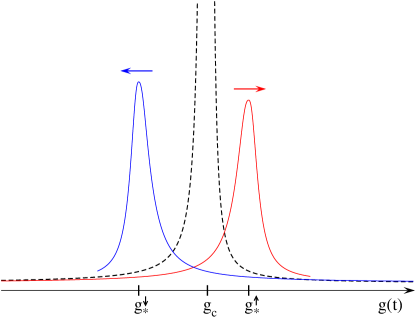
Figure 1: Schematic plot of our scheme for determination of the quantum critical point $g_{c}$. Dashed lines show the equilibrium susceptibility, which is divergent at $g_{c}$. The red (blue) line shows the non-equilibrium susceptibility for the quench, where the parameter $g$ is ramped up (down). Arrows indicate the direction of changes of $g(t)$. The quantum critical point is supposed to be located between the extrema of these curves, $g_{*}^{\downarrow}<g_{c}<g_{*}^{\uparrow}$.

This qualitative description can be made quantitative with the KZ theory, which introduces the characteristic non-equilibrium time scale $\hat{t}\sim\tau_{Q}^{z\nu/(1+z\nu)}$ and the interrelated field scale

$$\hat{g}=|g(t_{c}\pm\hat{t}\,)-g_{c}|\sim\tau_{Q}^{-1/(1+z\nu)},$$ (3)

where $z$ and $\nu$ are the dynamical and correlation-length universal critical exponents. It can be then argued that near the QCP, the non-equilibrium susceptibility $\chi$ will be dominated, for slow-enough quenches, by its universal part

$$\chi(g(t))\approx\hat{\chi}f\!\left(\frac{g(t)-g_{c}}{\hat{g}}\right),$$ (4)

$$\hat{\chi}=\chi^{eq}[g(t_{c}\pm\hat{t}\,)]\sim\tau_{Q}^{\gamma/(1+z\nu)},$$

where $f(x)$ is a non-singular scaling function, which is proportional to $|x|^{-\gamma}$ before the onset of non-equilibrium dynamics, so that $\chi(g(t))\approx\chi^{eq}_{sing}(g(t))$ there. Ansatz (4) combines two basic ingredients of the KZ theory. First, the adiabatic-impulse approximation assuming that system’s dynamics is frozen in the impulse regime, i.e. when $|t-t_{c}|<\hat{t}$, and adiabatic before entering it BDP (a, b); Tomka et al. (2018). This introduces $\hat{\chi}$ into (4). Second, the assumption that non-equilibrium dynamics of physical observables should depend on the rescaled time difference $(t-t_{c})/\hat{t}$, which explains the scaling function in (4). The latest take on this ansatz can be found in Kol ; Son ; Fra ; Sadhukhan et al. (2020); Rossini and Vicari (2020), see e.g. BDP (c) for preceding work in the context of classical phase transitions.

It now follows from (4) that precision of QCP determination should increase with the quench time as

$$\delta=g_{*}^{\uparrow}-g_{*}^{\downarrow}\sim\tau_{Q}^{-1/(1+z\nu)}.$$ (5)

Several remarks are in order now.

First, we propose that the above-outlined scheme can be used for either numerical or experimental localization of QCPs.

Second, arguments presented between (1) and (3) are based on general considerations, which do not involve the KZ theory. For this reason, they should be presumably more robust than KZ predictions, which are laid out in (4) and (5). So, even in systems where quantitative verification of the KZ theory is challenging, our technique for localization of QCPs may still be useful.

Third, it is interesting to realize that just a single, in each direction, sweep of the parameter driving the transition may be sufficient for reasonably-accurate estimation of the position of the QCP. Note that one cannot get both upper and lower bounds on the position of the QCP from a single one-way quench. Our two-way quench protocol gets around this limitation.

Fourth, our scheme does not specify, where the QCP is located between the maxima of non-equilibrium susceptibilities, i.e. within the interval $(g_{*}^{\downarrow},g_{*}^{\uparrow})$. The fact, that the position of the QCP is supposed to be bounded in such a way, could be of practical relevance, because features such as extrema are typically the easiest to extract from experimental data. However, if determination of some susceptibility would require differentiation of such presumably noisy data, one will have to smooth that data first. This can be done with various techniques, see e.g. BDS for the Padé approximant example.

Fifth, result (5) is of interest from the metrological perspective and it is worth to stress that the KZ theory has been only recently systematically explored in the metrological context Rams et al. (2018). Moreover, (5) can be also used for extracting the product of universal critical exponents.

Two exactly solvable models will be used below for illustration of above-introduced concepts. Their numerical solutions will be presented on Figs. 2–7. Technical details of our simulations can be found in Appendices A and B.

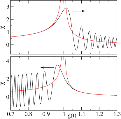
Figure 2: Dynamics of the susceptibility $\chi(g(t))$ during up and down quenches in the extended $XY$ model is presented by black lines in upper and lower panels, respectively. The instantaneous equilibrium value of the susceptibility, $\chi^{eq}(g(t))$, is provided by red lines. The quench time $\tau_{Q}=300$.

III Extended $XY$ model

We take the Hamiltonian

$$H=-\sum_{i=1}^{N}(\sigma_{i}^{x}\sigma_{i+1}^{x}+\tfrac{1}{3}\sigma_{i}^{y}\sigma_{i+1}^{y}-\tfrac{1}{3}\sigma_{i}^{x}\sigma_{i+1}^{z}\sigma_{i+2}^{x}+g\sigma_{i}^{z}),$$ (6)

where $g\geq 0$ is the external magnetic field, $\sigma^{x,y,z}_{i}$ are Pauli matrices acting on the $i$-th spin, $N$ is the number of spins, and periodic boundary conditions are implemented. Basic properties of this model were described in Suzuki (1971); Sadhukhan et al. (2020). Its QCP is at $g_{c}=1$ and it separates ferromagnetic ($0<g<1$) and paramagnetic ($g>1$) phases. Critical exponents of (6) are $z=3$ and $\nu=1/3$.

As the susceptibility of interest in our translationally-invariant system, we take the derivative of the transverse magnetization at an arbitrary lattice site

$$\chi=\frac{d\langle\sigma^{z}_{i}\rangle}{dg}.$$ (7)

In equilibrium, this quantity is algebraically divergent at the QCP. Indeed, $\chi^{eq}=-d^{2}E_{0}/dg^{2}$ from the Feynman-Hellmann theorem, where $E_{0}$ is the ground state energy per lattice site. The singular part of $E_{0}$ is typically assumed to scale as $|g-g_{c}|^{2-\alpha}$. If we now combine this insight with the quantum hyperscaling relation–i.e. $\alpha=2-\nu(d+z)$, where $d$ represents system dimensionality Con –we will get that $\alpha=2/3$ for model (6). Thus, $\chi^{eq}_{sing}(g)$ is given by (1) with $g_{c}=1$ and $\gamma=2/3$, which we have numerically verified, and so $\hat{\chi}\sim\tau_{Q}^{1/3}$.

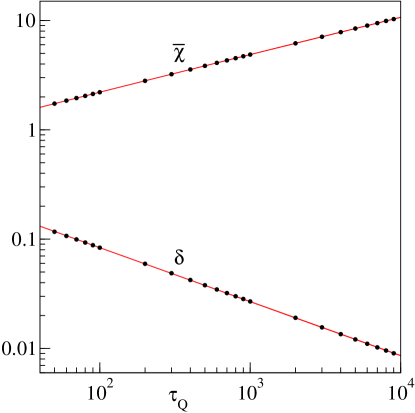
Figure 3: Global maxima of the non-equilibrium susceptibility $\chi$ of the extended $XY$ model. Upper data: the average value of $\chi$ at global maxima during up and down quenches. Lower data: the distance $\delta$ between such maxima. Red lines show fits to black dots coming from numerics, see (10) and (11).

The ramp up of the magnetic field will be done with

$$g(t)=\!\left(\frac{t}{2\tau_{Q}}\right)^{2},$$ (8)

while its ramp down will be done with

$$g(t)=g_{0}-\frac{t}{\tau_{Q}},\ g_{0}=5.$$ (9)

Both quenches start from ground states at $t=0$ and then the system is driven towards the QCP, which is reached at $t_{c}$ equal to $2\tau_{Q}$ and $(g_{0}-1)\tau_{Q}$ for up (8) and down (9) quenches, respectively.

These quenches share the same important property. Namely, their rate, given by $|dg/dt|$, is equal to $\tau_{Q}^{-1}$ at $t_{c}$. Thus, near the QCP, the driving proceeds just as in model quench (2), which is all that should matter in the context of the KZ theory (see e.g. BDN for a similar quadratic-in-time quench studied in the KZ framework).

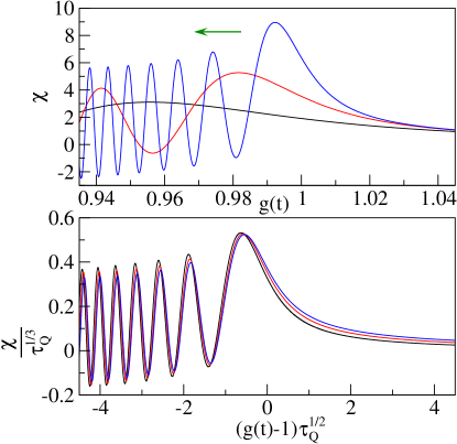
Figure 4: Dynamics of the susceptibility $\chi$ during down quenches of the extended $XY$ model. Black, red, and blue lines are obtained for $\tau_{Q}=200$, $1000$, and $5000$, respectively. Panels show results before and after KZ rescalings.

As for differences between (8) and (9), we note that quenches typically produce excitations at the beginning of time evolution (see e.g. Mar ). Such excitations are of no interest in our studies. They appear because variations of the external parameter are not smoothly turned on (the more low-order derivatives of the external parameter vanish at $t=0$, the more adiabatic the quench initially is). Quadratic time dependence in (8) noticeably reduces initial excitation of our system with respect to what would happen if the up quench would be linear. The situation is somewhat similar for down quenches (9). However, the gap in the excitation spectrum is much larger at $g_{0}\gg 1$ than at $g=0$. Even for linear quenches, we find that it sufficiently reduces initial non-adiabaticity of our observable during “down” evolutions (the same happens in the Ising model studied in Sec. IV).

Typical dynamics of susceptibility (7) is presented in Fig. 2, where we see three distinct regimes. First, the evolution is adiabatic. Then, near the QCP, the susceptibility lags behind its instantaneous equilibrium value, and a well visible global maximum appears after crossing the QCP. Finally, the susceptibility oscillates, which can be regarded as a quasi-adiabatic stage (no more excitations are generated, system’s dynamics revolves around the instantaneous equilibrium solution).

More quantitatively, from numerical data presented in Fig. 3, we find that the distance $\delta$ between global maxima for up and down quenches is described by

$$\ln\delta=-0.209(3)-0.4936(5)\ln\tau_{Q}.$$ (10)

This result comes from a linear regression Reg . It is in excellent agreement with (5) suggesting a prefactor of $-1/2$ in front of the logarithm.

It is also instructive to have a look at the average value of the susceptibility at global maxima, which we denote by $\chi_{*}^{\uparrow}$ and $\chi_{*}^{\downarrow}$ for up and down quenches, respectively. The nonlinear fit to data from Fig. 3 shows that

$$\overline{\chi}=(\chi_{*}^{\uparrow}+\chi_{*}^{\downarrow})/2=-0.063(2)+0.4795(7)\tau_{Q}^{0.3376(2)},$$ (11)

where the exponent is in excellent agreement with the value of $1/3$ due to $\gamma=2/3$ and $z\nu=1$ (4). Similar results are obtained when the fit is individually performed for either $\chi_{*}^{\uparrow}$ or $\chi_{*}^{\downarrow}$. Computation of $\overline{\chi}$, however, removes small deviations of $\chi_{*}^{\uparrow}$ and $\chi_{*}^{\downarrow}$ from the perfect KZ scaling solution. Those deviations are presumably caused by non-universal contributions to susceptibilities (see lower panel of Fig. 4, where collapse of global maxima, after KZ rescalings, is not exact and note that the KZ theory overlooks non-universal dynamics). Analogical remarks apply to the discussion of $\overline{\chi}$ in Sec. IV, and so they will not be repeated there.

Finally, we mention that ansatz (4) is verified in Fig. 4, where good overlap between non-equilibrium susceptibilities, obtained for vastly different quench times $\tau_{Q}$, is seen after proper rescalings.

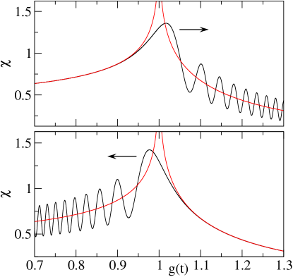
Figure 5: Black lines: the susceptibility $\chi(g(t))$ during up (upper panel) and down (lower panel) quenches of the Ising model with $\tau_{Q}=300$. Red lines: the instantaneous equilibrium value of $\chi$.

IV Ising model

The Hamiltonian of interest now is

$$H=-\sum_{i=1}^{N}(\sigma^{x}_{i}\sigma^{x}_{i+1}+g\sigma^{z}_{i}),$$ (12)

where the QCP and phases are the same as in the extended $XY$ chain Lie ; Pfe ; BDJ . Dynamics of this paradigmatic model, under continuous driving such as (2), was studied in Jac (b); Dor (a); Pol (b); Ral ; Pol (c); Sen (a); San (a); Jac (c); Sen (b); Arn (b); Kol ; Yin et al. ; Dut ; Fra ; San (b); BDp ; Pus ; Apo ; Mic (a); Ado ; Mar ; Mic (b). Key differences between (6) and (12) are seen through critical exponents, which are now given by $z=\nu=1$.

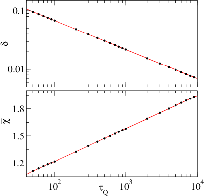
Figure 6: Upper panel: the distance $\delta$ between global maxima of the susceptibility $\chi$ appearing during up and down quenches of the Ising model. Lower panel: arithmetic average of the value of $\chi$ at those maxima. Black dots show numerics, red lines are fits (15) and (16).

Such values lead to non-algebraic singularity of the equilibrium version of susceptibility (7), which can be understood by noting that $\alpha=0$ now. Indeed, $\chi^{eq}_{sing}$ has the following expansion near the QCP Lac

$$\chi^{eq}_{sing}(g)\approx-\frac{1}{\pi}\ln|g-1|.$$ (13)

This well-known result is a bit unusual because one typically expects algebraic singularities as in (1). Logarithmic singularity of $\chi^{eq}_{sing}$ has interesting consequences on $\chi$, whose scaling properties are not captured by (4). The appropriate KZ ansatz reads

$$\chi(g(t))\approx f\!\left(\frac{g(t)-g_{c}}{\hat{g}}\right)+\frac{\ln\tau_{Q}}{2\pi},$$ (14)

where up to a constant term, $f(x)$ is approximated by $-\frac{1}{\pi}\ln|x|$ before the onset of non-equilibrium dynamics. To derive (14), we start with $d^{2}\langle\sigma^{z}_{i}\rangle/dg^{2}$, whose equilibrium value is algebraically divergent at the QCP, apply ansatz (4) to it, integrate the resulting expression, and take into account adiabaticity before the beginning of non-equilibrium dynamics (see Appendix C for a detailed discussion). Alternatively, one may adopt results from Lac , where $d\langle\sigma^{z}_{i}\rangle/dg$ was studied with renormalization group techniques in a time-independent but spatially inhomogeneous Ising chain. This is done by replacing $\lambda_{Q}$ with $\tau_{Q}$ in Eq. (26) from Lac . Finally, it may be also worth to mention that, to the best of our knowledge, scaling ansatz (14) has never been applied to time quenches before.

Typical dynamics of the susceptibility $\chi$, due to either (8) or (9), is shown in Fig. 5. The fits from Fig. 6 are

$$\ln\delta=-0.397(3)-0.4965(4)\ln\tau_{Q},$$ (15)

$$\overline{\chi}=0.495(2)+0.1575(2)\ln\tau_{Q},$$ (16)

which can be compared to our theory. The prefactor in front of the logarithm in (15) should be $-1/2$, and indeed it is very much so. The one in (16) is also very close to our expectations, i.e. $1/2\pi\approx 0.159$ due to (14). Finally, verification of ansatz (14) is shown in Fig. 7, where pretty good overlap between curves is found.

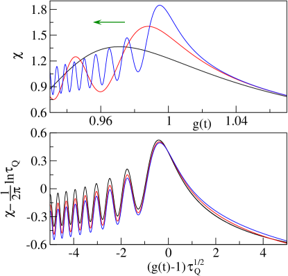
Figure 7: Dynamics of the susceptibility $\chi$ during down quenches of the Ising model: before and after KZ rescalings motivated by ansatz (14). Black, red, and blue lines are obtained for $\tau_{Q}=200$, $1000$, and $5000$.

V Conclusions

Summarizing, we have proposed how quantum critical points can be accurately localized by scanning a non-equilibrium susceptibility during Kibble-Zurek quenches. Our scheme assumes that two such scans are performed by either increasing or decreasing the external parameter driving the transition. We have argued that each of them should lead to formation of a peak of a non-equilibrium susceptibility, and that the critical point can be pinned down to the interval marked off by these values of the external parameter, at which the peaks are observed. The width of such an interval has been argued to exhibit universal power-law scaling with the quench time, shrinking to zero in the adiabatic limit.

We have tested these predictions in two exactly solvable models, exhibiting either algebraic or logarithmic singularities of equilibrium susceptibilities. We have found that each quench actually produces a train of progressively smaller susceptibility peaks. By focusing on the highest one for each quench, our expectations have been precisely confirmed. There are several prospective extensions of these studies.

First, similar calculations can be done in other models. This should increase understanding of susceptibilities during Kibble-Zurek quenches. This is arguably a poorly explored topic as we have been able to find only three references exploring susceptibilities in the Kibble-Zurek context Yin et al. ; Lac ; Mar . Out of them, Lac is not even focused on non-equilibrium dynamics of the kind we discuss in this work as it deals with spatial Kibble-Zurek quenches Tur ; Dor (b). It should be also noted that as long as $\tau_{Q}<\infty$, there will be always non-universal contributions to dynamics of susceptibilities, which are not captured by the Kibble-Zurek theory. Their quantification requires system-specific studies.

Second, our scheme can be used for numerical localization of quantum critical points in non-exactly solvable models, providing a complementary approach to studies based on evaluation of equilibrium susceptibilities. This complementarity can be seen by noting that generation of quantum states, used for computation of equilibrium (non-equilibrium) susceptibilities, can be done by imaginary (real) time evolutions. It can be also seen from the perspective of tensor network simulations Verstraete et al. (2008); Schollwöck (2011); Orús (2014), where equilibrium calculations can be done with variational methods, while the non-equilibrium ones, needed for exploration of our scheme, would follow from their time-dependent extensions.

Third, we expect that our predictions could be used for experimental determination of phase diagrams of physical systems through their non-equilibrium response to variations of external fields. They could also motivate experimental studies of susceptibilities during Kibble-Zurek quenches. In particular, one should be able to implement and test our scheme in cold atom and ion emulators of spin systems Por ; Kor ; Lew ; Blo ; Sch , whose dynamical experimental studies were recently reported in Luk (a); Mon ; Luk (b); LMG . The important open question here is how robust our approach is to environmental couplings and “imperfections” of real experimental setups.

Finally, we would also like to mention that similar phenomena may be also noticeable during non-equilibrium classical phase transitions. We think so because the Kibble-Zurek theory similarly describes dynamics of quantum and classical systems Kibble (2007); Jac (a); Pol (a); del (a, b). In fact, it was originally developed in the classical context Kib ; Zur . Thus, extension of our studies to various systems undergoing classical phase transitions, such as those listed at the very beginning of this work, looks to us like a promising research direction.

Appendix A Numerical simulations of Ising model

We will outline here basic steps leading to efficient numerical simulations of periodic Ising model (12).

To begin, we note that Hamiltonian (12) commutes with the parity operator $\prod^{N}_{i=1}\sigma^{z}_{i}$, whose eigenvalues are $\pm 1$. This leads to splitting of the Hilbert space into positive- and negative-parity subspaces, where eigenstates of $H$ have either $+1$ or $-1$ parity. Moreover, the parity of the system’s state is preserved during time evolutions. Our evolutions start from ground states in the positive-parity subspace. Moreover, we consider systems composed of an even number of spins, which simplifies a bit the following discussion (see BDJ for a comprehensive discussion of the impact of the parity and system size on the spin-to-fermion mapping that we employ below).

The following discussion is conveniently carried out by mapping spins onto non-interacting fermions via the Jordan-Wigner transformation

$$\sigma^{z}_{i}=1-2c_{i}^{\dagger}c_{i},\ \sigma^{x}_{i}=(c_{i}+c_{i}^{\dagger})\prod_{j<i}(1-2c_{j}^{\dagger}c_{j}),$$ (17)

$$\{c_{i},c_{j}^{\dagger}\}=\delta_{ij},\ \{c_{i},c_{j}\}=0,$$

where anti-periodic boundary conditions have to be imposed on the fermionic operators $c_{i}$ because we work in the positive-parity subspace Jac (b); BDJ .

One then goes to the momentum space through the substitution

$$c_{j}=\frac{\exp(-\mathrm{i}\pi/4)}{\sqrt{N}}\sum_{K=\pm k}c_{K}\exp(\mathrm{i}Kj),$$ (18)

$$k=\frac{\pi}{N},\frac{3\pi}{N},\cdots,\pi-\frac{\pi}{N},$$

arriving at

$$H=2\sum_{k}\big{[} (c_{k}^{\dagger}c_{k}-c_{-k}c_{-k}^{\dagger})(g-\cos k)$$ (19)

$$+ (c_{k}^{\dagger}c_{-k}^{\dagger}+c_{-k}c_{k})\sin k\big{]},$$

which can be diagonalized via the Bogolubov transformation. The ground state of (19) is

$$|g\rangle=\prod_{k}(u_{k}^{eq}-v_{k}^{eq}c_{k}^{\dagger}c_{-k}^{\dagger})|{\rm vac}\rangle,$$ (20)

$$u_{k}^{eq}=\cos\frac{\theta_{k}}{2},\ v_{k}^{eq}=\sin\frac{\theta_{k}}{2},$$ (21)

$$\sin\theta_{k}=\frac{\sin k}{\sqrt{g^{2}-2g\cos k+1}},$$ (22)

$$\cos\theta_{k}=\frac{g-\cos k}{\sqrt{g^{2}-2g\cos k+1}},$$ (23)

where the vacuum state $|{\rm vac}\rangle$ is annihilated by all $c_{\pm k}$ operators.

From the time-dependent Schrödinger equation,

$$\mathrm{i}\frac{d}{dt}|\psi(t)\rangle=H[g(t)]|\psi(t)\rangle,$$ (24)

one then finds that Jac (b)

$$|\psi(t)\rangle=\prod_{k}(u_{k}(t)-v_{k}(t)c_{k}^{\dagger}c_{-k}^{\dagger})|{\rm vac}\rangle,$$ (25)

$$\mathrm{i}\frac{d}{dt}\left(\begin{array}[]{c}v_{k}\\ u_{k}\end{array}\right)=2\left(\begin{array}[]{cc}g(t)-\cos k&-\sin k\\ -\sin k&\cos k-g(t)\end{array}\right)\left(\begin{array}[]{c}v_{k}\\ u_{k}\end{array}\right).$$ (32)

The above differential equations are efficiently numerically solved with standard techniques (we use the Bulirsch-Stoer method Rec ). The initial conditions are chosen such that $u_{k}$ and $v_{k}$, at the beginning of time evolution, are equal to $u_{k}^{eq}$ and $v_{k}^{eq}$, respectively. The latter are computed at the initial value of the magnetic field.

The non-equilibrium transverse magnetization is given by

$$S^{z}(g(t))=\langle\psi(t)|\sigma^{z}_{i}|\psi(t)\rangle=1-\frac{4}{N}\sum_{k}|v_{k}(t)|^{2}.$$ (33)

Its equilibrium value is obtained after the replacements $|\psi(t)\rangle\to|g\rangle$ and $v_{k}(t)\to v^{eq}_{k}$. From (33), the non-equilibrium susceptibility $\chi$ is numerically computed via

$$\chi(g_{i+1/2})=\chi\!\left(g_{i}+\frac{g_{i+1}-g_{i}}{2}\right)\approx\frac{S^{z}(g_{i+1})-S^{z}(g_{i})}{g_{i+1}-g_{i}},$$ (34)

where $g_{i}=g(t_{i})$. The grid, which we use for computation of this quantity, is $g_{i+1}-g_{i}=5\cdot 10^{-5}$. The equilibrium susceptibility $\chi^{eq}$ is trivially computed through analytic differentiation.

We identify positions of maxima of the non-equilibrium susceptibility in the following way. First, we choose $\tau_{Q}$ and find the global maximum on the susceptibility vs. magnetic field plot, say at $(g_{j+1/2},\chi(g_{j+1/2}))$. We then fit a parabola to the points $(g_{i+1/2},\chi(g_{i+1/2}))$ around it, satisfying $\chi(g_{i+1/2})\geq\chi(g_{j+1/2})(1-\epsilon)$, where $\epsilon=0.0025$ is chosen (the twice larger $\epsilon$ gives essentially identical results). The maximum of such obtained parabola is then analyzed in the main body of this paper. The fitting procedure makes our results independent of tiny oscillations of data points. It also allows for interpolation of positions of maxima between the grid points.

Our numerics, presented in the main text, have been done for systems composed of $N=2000$ spins. This imposes an upper limit on quench times, for which Kibble-Zurek dynamics should be free from finite-size effects. Namely, the size of the system should be much larger than the correlation length around the time, when the system goes out of equilibrium Jac (a). The latter is proportional to $\tau_{Q}^{\nu/{(1+z\nu)}}$ Dor (a); Jac (a). So, this condition leads to $\tau_{Q}\ll N^{2}$ in the Ising chain, which is satisfied in all our numerical simulations. In accordance with these expectations, we have directly verified that virtually identical results, to those reported in the main text, are also obtained when $N=1000$. Finally, in the main body of our work, we do the fits to numerics in the range $50\leq\tau_{Q}\leq 9000$.

Appendix B Numerical simulations of extended $XY$ model

The procedure, leading to efficient numerical simulations of periodic extended $XY$ model (6), is similar to the one discussed in Appendix A. Therefore, we list below only differences between our treatment of the two models and their properties.

To start, we mention that Jordan-Wigner transformation (17) has to be supplemented by $\sigma^{y}_{i}=\mathrm{i}(c_{i}^{\dagger}-c_{i})\prod_{j<i}(1-2c_{j}^{\dagger}c_{j})$. Then, introducing

$$A_{k}(g)=g-\tfrac{4}{3}\cos k+\tfrac{1}{3}\cos 2k,$$ (35)

$$B_{k}=\tfrac{2}{3}\sin k-\tfrac{1}{3}\sin 2k,$$

we can concisely state that (19), (22), (23), and (32), get now replaced by

$$H=2\sum_{k}\big{[} (c_{k}^{\dagger}c_{k}-c_{-k}c_{-k}^{\dagger})A_{k}(g)$$ (36)

$$+ (c_{k}^{\dagger}c_{-k}^{\dagger}+c_{-k}c_{k})B_{k}\big{]},$$

$$\sin\theta_{k}=\frac{B_{k}}{\sqrt{A_{k}^{2}(g)+B^{2}_{k}}},$$ (37)

$$\cos\theta_{k}=\frac{A_{k}(g)}{\sqrt{A_{k}^{2}(g)+B_{k}^{2}}},$$ (38)

and

$$\mathrm{i}\frac{d}{dt}\left(\begin{array}[]{c}v_{k}\\ u_{k}\end{array}\right)=2\left(\begin{array}[]{cc}A_{k}(g(t))&-B_{k}\\ -B_{k}&-A_{k}(g(t))\end{array}\right)\left(\begin{array}[]{c}v_{k}\\ u_{k}\end{array}\right),$$ (39)

respectively. The last difference is that the condition for finite-size-independence of KZ dynamics now reads $\tau_{Q}\ll N^{6}$, because $z=3$ and $\nu=1/3$ in this model Sadhukhan et al. (2020). We mention in passing that there are misprints in the expression for (36) in Sadhukhan et al. (2020).

The rest of the discussion from whole Appendix A identically characterizes our studies of the extended $XY$ model.

Appendix C Scaling ansatz for susceptibility of Ising model

To support the scaling ansatz for the susceptibility $\chi$ of the Ising model, we start from consideration of

$$\tilde{\chi}=\frac{d\chi}{dg}.$$ (40)

Its equilibrium singular part is given by

$$\tilde{\chi}^{eq}_{sing}\approx\frac{1}{\pi(1-g)},$$ (41)

and so $\tilde{\chi}^{eq}$ is algebraically divergent at the QCP. Applying to (40) scaling ansatz (4), we get

$$\tilde{\chi}\approx\sqrt{\tau_{Q}}\tilde{f}((g-1)\sqrt{\tau_{Q}}),$$ (42)

which, when combined with (40), leads to

$$\frac{d\chi}{dx}\approx\tilde{f}(x),\ \ x=(g-1)\sqrt{\tau_{Q}}.$$ (43)

Integrating (43) over $x$, we get

$$\chi\approx h(x)+C,$$ (44)

where $h$ is a new scaling function. To fix the $x$-independent $C$ term, we require that $\chi(x\ll-1)$ for the up quench and $\chi(x\gg 1)$ for the down quench are well-approximated by

$$\chi^{eq}_{sing}\approx-\frac{1}{\pi}\ln|g-1|.$$ (45)

Then, we note that by definition scaling functions can depend on $\tau_{Q}$ only through their argument. This leads to the conclusion that

$$\chi\approx h((g-1)\sqrt{\tau_{Q}})+\frac{\ln\tau_{Q}}{2\pi},$$ (46)

where $h(x\ll-1)$ for the up quench and $h(x\gg 1)$ for the down quench are well-approximated by $-\frac{1}{\pi}\ln|x|$. After identification of $h((g-1)\sqrt{\tau_{Q}})$ with $f((g(t)-g_{c})/\hat{g})$, (46) matches (14). We mention in passing that a factor of $2$, in the denominator of the second term in (46), can be traced back to $1+z\nu=2$.

References

- (1) T. W. B. Kibble, Phys. Rep. 67,183 (1980).
- (2) W. H. Zurek, Phys. Rep. 276, 177 (1996).
- Kibble (2007) T. Kibble, Phys. Today 60, 47 (2007).
- Jac (a) J. Dziarmaga, Adv. Phys. 59, 1063 (2010).
- Pol (a) A. Polkovnikov, K. Sengupta, A. Silva, and M. Vengalattore, Rev. Mod. Phys. 83, 863 (2011).
- del (a) A. del Campo, T. W. B. Kibble, and W. H. Zurek, J. Phys.: Condens. Matter 25, 404210 (2013).
- del (b) A. del Campo and W. H. Zurek, Int. J. Mod. Phys. A 29, 1430018 (2014).
- (8) J. Cardy, Scaling and Renormalization in Statistical Physics (Cambridge University Press, Cambridge, 2002).
- Coleman and Schofield (2005) P. Coleman and A. J. Schofield, Nature 433, 226 (2005).
- Sac (a) S. Sachdev, Quantum Phase Transitions (Cambridge University Press, 2011).
- (11) M. Continentino, Quantum Scaling in Many-Body Systems: An Approach to Quantum Phase Transitions (Cambridge University Press, 2nd edition, 2017).
- Sac (b) S. Sachdev and B. Keimer, Phys. Today 64, 29 (2011).
- BDP (a) B. Damski, Phys. Rev. Lett. 95, 035701 (2005).
- Dor (a) W. H. Zurek, U. Dorner, and P. Zoller, Phys. Rev. Lett. 95, 105701 (2005).
- Jac (b) J. Dziarmaga, Phys. Rev. Lett. 95, 245701 (2005).
- (16) S. Yin, X. Qin, C. Lee, and F. Zhong, eprint arXiv:1207.1602 (2013).
- Hu et al. (2015) Q. Hu, S. Yin, and F. Zhong, Phys. Rev. B 91, 184109 (2015).
- Huang and Yin (2019) R.-Z. Huang and S. Yin, Phys. Rev. B 99, 184104 (2019).
- Arn (a) S. Bhattacharyya, S. Dasgupta, and A. Das, Sci. Rep. 5, 16490 (2015).
- Roy et al. (2017) S. Roy, R. Moessner, and A. Das, Phys. Rev. B 95, 041105(R) (2017).
- BDP (b) B. Damski and W. H. Zurek, Phys. Rev. A 73, 063405 (2006).
- Tomka et al. (2018) M. Tomka, L. Campos Venuti, and P. Zanardi, Phys. Rev. A 97, 032121 (2018).
- (23) M. Kolodrubetz, B. K. Clark, and D. A. Huse, Phys. Rev. Lett. 109, 015701 (2012).
- (24) A. Chandran, A. Erez, S. S. Gubser, and S. L. Sondhi, Phys. Rev. B 86, 064304 (2012).
- (25) A. Francuz, J. Dziarmaga, B. Gardas, and W. H. Zurek, Phys. Rev. B 93, 075134 (2016).
- Sadhukhan et al. (2020) D. Sadhukhan, A. Sinha, A. Francuz, J. Stefaniak, M. M. Rams, J. Dziarmaga, and W. H. Zurek, Phys. Rev. B 101, 144429 (2020).
- Rossini and Vicari (2020) D. Rossini and E. Vicari, Phys. Rev. Research 2, 023211 (2020).
- BDP (c) B. Damski and W. H. Zurek, Phys. Rev. Lett. 104, 160404 (2010).
- (29) O. A. Prośniak, M. Łącki, and B. Damski, Sci. Rep. 9, 8687 (2019).
- Rams et al. (2018) M. M. Rams, P. Sierant, O. Dutta, P. Horodecki, and J. Zakrzewski, Phys. Rev. X 8, 021022 (2018).
- Suzuki (1971) M. Suzuki, Prog. Theor. Phys. 46, 1337 (1971).
- (32) B. Damski and W. H. Zurek, New J. Phys. 10, 045023 (2008).
- (33) M. M. Rams, J. Dziarmaga, and W. H. Zurek, Phys. Rev. Lett. 123, 130603 (2019).
- (34) One standard error, delivered by NonlinearModelFit function from Mat , is provided in brackets in all our fitting results.
- (35) E. Lieb, T. Schultz, and D. Mattis, Ann. Phys. (N.Y.) 16, 407 (1961).
- (36) P. Pfeuty, Ann. Phys. 57, 79 (1970).
- (37) B. Damski and M. M. Rams, J. Phys. A 47, 025303 (2014).
- Pol (b) A. Polkovnikov, Phys. Rev. B 72, 161201(R) (2005).
- (39) S. Mostame, G. Schaller, and R. Schützhold, Phys. Rev. A 76, 030304(R) (2007).
- Pol (c) R. Barankov and A. Polkovnikov, Phys. Rev. Lett. 101, 076801 (2008).
- Sen (a) S. Mondal, K. Sengupta, and D. Sen, Phys. Rev. B 79, 045128 (2009).
- San (a) D. Patanè, L. Amico, A. Silva, R. Fazio, and G. E. Santoro, Phys. Rev. B 80, 024302 (2009).
- Jac (c) L. Cincio, J. Dziarmaga, M. M. Rams, and W. H. Zurek, Phys. Rev. A 75, 052321 (2007).
- Sen (b) K. Sengupta and D. Sen, Phys. Rev. A 80, 032304 (2009).
- Arn (b) A. Das, Phys. Rev. B 82, 172402 (2010).
- (46) A. Dutta, G. Aeppli, B. K. Chakrabarti, U. Divakaran, T. F. Rosenbaum, and D. Sen, Quantum Phase Transitions in Transverse Field Spin Models: From Statistical Physics to Quantum Information (Cambridge University Press, 2015).
- San (b) A. Russomanno, S. Sharma, A. Dutta, and G. E. Santoro, J. Stat. Mech. (2015) P08030.
- (48) B. Damski, Fidelity approach to quantum phase transitions in quantum Ising model, in Quantum Criticality in Condensed Matter: Phenomena, Materials and Ideas in Theory and Experiment, edited by J. Jedrzejewski (World Scientific, Singapore, 2015), pp. 159–182; arXiv:1509.03051.
- (49) T. Puskarov and D. Schuricht, SciPost Phys. 1, 003 (2016).
- (50) S. Lorenzo, J. Marino, F. Plastina, G. M. Palma, and T. J. G. Apollaro, Sci. Rep. 7, 5672 (2017).
- Mic (a) M. Białończyk and B. Damski, J. Stat. Mech. (2018) 073105.
- (52) A. del Campo, Phys. Rev. Lett. 121, 200601 (2018).
- Mic (b) M. Białończyk and B. Damski, J. Stat. Mech. (2020) 013108.
- (54) M. Łącki and B. Damski, J. Stat. Mech. (2017) 103105.
- (55) T. Platini, D. Karevski, and L. Turban, J. Phys. A: Math. Theor. 40, 1467 (2007).
- Dor (b) W. H. Zurek and U. Dorner, Phil. Trans. R. Soc. A 366, 2953 (2008).
- Verstraete et al. (2008) F. Verstraete, V. Murg, and J. Cirac, Adv. Phys. 57, 143 (2008).
- Schollwöck (2011) U. Schollwöck, Ann. Phys. 326, 96 (2011).
- Orús (2014) R. Orús, Ann. Phys. 349, 117 (2014).
- (60) D. Porras and J. I. Cirac, Phys. Rev. Lett. 92, 207901 (2004).
- (61) S. Korenblit et al., New J. Phys. 14, 095024 (2012).
- (62) M. Lewenstein, A. Sanpera, V. Ahufinger, B. Damski, A. Sen De, and U. Sen, Adv. Phys. 56, 243 (2007).
- (63) C. Gross and I. Bloch, Science 357, 995 (2017).
- (64) P. Schauss, Quantum Sci. Technol. 3, 023001 (2018).
- Luk (a) H. Bernien et al., Nature 551, 579 (2017).
- (66) J. Zhang, G. Pagano, P. W. Hess, A. Kyprianidis, P. Becker, H. Kaplan, A. V. Gorshkov, Z.-X. Gong, and C. Monroe, Nature 551, 601 (2017).
- Luk (b) A. Keesling et al., Nature 568, 207 (2019).
- (68) V. Makhalov, T. Satoor, A. Evrard, T. Chalopin, R. Lopes, and S. Nascimbene, Phys. Rev. Lett. 123, 120601 (2019).
- (69) W. H. Press, S. A. Teukolsky, W. T. Vetterling, and B. P. Flannery, Numerical recipes in C. The art of scientific computing (Cambridge University Press, 2nd edition, 1992).
- (70) Wolfram Research, Inc., Mathematica, Version 12.0, Champaign, IL (2019).