A compatible embedded-hybridized discontinuous Galerkin method

for the Stokes–Darcy-transport problem

Aycil Cesmelioglu and Sander Rhebergen

Abstract

We present a stability and error analysis of an embedded-hybridized discontinuous Galerkin (EDG-HDG) finite element method for coupled Stokes–Darcy flow and transport. The flow problem, governed by the Stokes–Darcy equations, is discretized by a recently introduced exactly mass conserving EDG-HDG method while an embedded discontinuous Galerkin (EDG) method is used to discretize the transport equation. We show that the coupled flow and transport discretization is compatible and stable. Furthermore, we show existence and uniqueness of the semi-discrete transport problem and develop optimal a priori error estimates. We provide numerical examples illustrating the theoretical results. In particular, we compare the compatible EDG-HDG discretization to a discretization of the coupled Stokes–Darcy and transport problem that is not compatible. We demonstrate that where the incompatible discretization may result in spurious oscillations in the solution to the transport problem, the compatible discretization is free of oscillations. An additional numerical example with realistic parameters is also presented.

Keywords: Stokes–Darcy flow, Coupled flow and transport, Beavers–Joseph–Saffman, Embedded and Hybridized methods, Discontinuous Galerkin, Multiphysics.

1 Introduction

The coupled Stokes–Darcy equations describe the interaction between free flow and flow in porous media. To model the transport of chemicals and contaminants in, for example, surface/subsurface flows, biochemical transport, or vascular hemodynamics problems, the Stokes–Darcy equations are coupled to a transport equation [14]. In this paper we consider one way coupling in which the velocity solution to the Stokes–Darcy flow problem is used in the transport equation to advect and diffuse a contaminant.

Many different finite element and mixed finite element [17, 28, 5, 7, 22, 6, 30], discontinuous Galerkin (DG) [8, 23, 24, 29, 34, 36], and hybridizable discontinuous Galerkin (HDG) [19, 20, 21, 27] methods have been proposed to discretize the Stokes–Darcy problem. Likewise, many different finite element methods have been proposed to discretize the transport equation, such as streamline diffusion, DG, and HDG methods [4, 11, 25, 26, 31, 41]. However, stability and accuracy of a discretization for the Stokes–Darcy problem and separately a discretization for the transport problem, does not guarantee that the coupled discretization for the Stokes–Darcy-transport problem will be stable and accurate. Examples of discontinuous Galerkin methods for the Stokes–Darcy-transport problem have been proposed in [35, 40]

To address the issue of coupling the discretization of a flow problem to the discretization of a transport problem, Dawson et al. [16] introduced the concept of compatibility; a discretization for flow and transport is compatible if it is globally conservative and zeroth-order accurate. They showed that loss of accuracy and/or loss of global conservation may occur if the discretization is not compatible. They furthermore showed that, for discontinuous Galerkin methods, compatibility is a stronger statement than local conservation of the flow field.

In this paper we discretize the Stokes–Darcy problem by an embedded-hybridized discontinuous Galerkin (EDG-HDG) finite element method [9]. The two main reasons to consider this discretization are: (i) mass is conserved exactly, i.e., the velocity field is divergence-conforming on the whole domain and mass is conserved point-wise; and (ii) the EDG-HDG discretization has fewer globally coupled degrees of freedom than traditional DG and HDG methods and is generally better suited to fast iterative solvers than HDG methods, as shown in [33]. We discretize the transport equation by an embedded discontinuous Galerkin (EDG) method [41], the main motivation being that EDG discretizations are generally computationally more efficient than DG and HDG discretizations. We will show that the EDG-HDG flow discretization is compatible with the EDG discretization of the transport equation. We prove well-posedness of the discrete transport problem and present optimal error estimates.

The outline for the remainder of this paper is as follows. In section 2 we describe the Stokes–Darcy flow system and its coupling to the transport problem. The compatible EDG-HDG discretization for the Stokes–Darcy-transport problem, together with some of its properties, is introduced in section 3. In section 4 we discuss useful inequalities that will be used to prove existence and uniqueness of a solution to the semi-discrete transport problem in section 5. Error estimates are developed for the semi-discrete transport scheme in section 6. In section 7 we verify the analysis by numerical experiments while conclusions are drawn in section 8.

2 The Stokes–Darcy system coupled to transport

Let $\Omega\subset\mathbb{R}^{\dim}$, ${\dim}=2,3$, be a bounded polygonal domain with boundary $\partial\Omega$ and boundary outward unit normal vector $n$. We assume the domain is divided into two non-overlapping polygonal subdomains, $\Omega^{s}$ and $\Omega^{d}$, such that $\Omega=\Omega^{s}\cup\Omega^{d}$. The interface separating these subdomains is denoted by $\Gamma^{I}$. Furthermore, for $j=s,d$, the outward unit normal vector of $\Omega^{j}$ is denoted by $n^{j}$ and the exterior boundary of $\Omega^{j}$ is denoted by $\Gamma^{j}=\partial\Omega\cap\Omega^{j}$. The Stokes–Darcy system for the velocity $u\mathrel{\mathop{\mathchar 58\relax}}\Omega\rightarrow\mathbb{R}^{\dim}$ and pressure $p\mathrel{\mathop{\mathchar 58\relax}}\Omega\rightarrow\mathbb{R}$ is given by

$$-\nabla\cdot 2\mu\varepsilon(u)+\nabla p =f^{s} \text{in}\ \Omega^{s},$$ (1a)

$$\kappa^{-1}u+\nabla p =0 \text{in}\ \Omega^{d},$$ (1b)

$$-\nabla\cdot u =\chi^{d}f^{d} \text{in}\ \Omega,$$ (1c)

$$u =0 \text{on}\ \Gamma^{s},$$ (1d)

$$u\cdot n =0 \text{on}\ \Gamma^{d},$$ (1e)

where $\varepsilon(u)=(\nabla u+\nabla u^{T})/2$ is the strain rate tensor, $\mu>0$ is the constant kinematic viscosity, $\kappa>0$ is the permeability constant, $f^{s}\mathrel{\mathop{\mathchar 58\relax}}\Omega^{s}\rightarrow\mathbb{R}^{\dim}$ is a forcing term, $f^{d}\mathrel{\mathop{\mathchar 58\relax}}\Omega^{d}\rightarrow\mathbb{R}$ is a source/sink term, and $\chi^{d}$ is the characteristic function of $\Omega^{d}$. In the following we will denote the restriction of $u$ and $p$ on $\Omega^{j}$ by $u^{j}$ and $p^{j}$, respectively, for $j=s,d$.

Let $n$ denote the unit normal vector on $\Gamma^{I}$ pointing outwards from $\Omega^{s}$, that is, $n=n^{s}=-n^{d}$. We denote the tangential component of a vector $w$ by $(w)^{t}\mathrel{\mathop{\mathchar 58\relax}}=w-(w\cdot n)n$. On the interface we then prescribe the following transmission conditions:

$$u^{s}\cdot n =u^{d}\cdot n \text{on}\ \Gamma^{I},$$ (2a)

$$p^{s}-2\mu\varepsilon(u^{s})n\cdot n =p^{d} \text{on}\ \Gamma^{I},$$ (2b)

$$-2\mu\mathinner{\left(\varepsilon(u^{s})n\right)}^{t} =\alpha\kappa^{-1/2}(u^{s})^{t} \text{on}\ \Gamma^{I},$$ (2c)

where $\alpha>0$ is an experimentally determined constant. Equations 2a and 2b denote balance of flux and normal stress, and eq. 2c is the Beavers–Joseph–Saffman interface condition [2, 37].

The Stokes–Darcy system described above is coupled to a transport equation over the time interval of interest $I=(0,T]$. Given a porosity constant $\phi$ such that $0<\phi\leq 1$ in $\Omega^{d}$ and $\phi=1$ in $\Omega^{s}$, velocity field $u\mathrel{\mathop{\mathchar 58\relax}}\Omega\to\mathbb{R}^{\dim}$, and source/sink term $f\mathrel{\mathop{\mathchar 58\relax}}\Omega\times I\rightarrow\mathbb{R}$, the transport equation for the concentration $c\mathrel{\mathop{\mathchar 58\relax}}\Omega\times I\rightarrow\mathbb{R}$ of a contaminant is given by:

$$\phi\partial_{t}c+\nabla\cdot(cu-D(u)\nabla c) =f \text{in}\ \Omega\times I,$$ (3a)

$$D(u)\nabla c\cdot n =0 \text{on}\ \partial\Omega\times I,$$ (3b)

$$c(x,0) =c_{0}(x) \text{in}\ \Omega,$$ (3c)

where $c_{0}\mathrel{\mathop{\mathchar 58\relax}}\Omega\rightarrow\mathbb{R}$ is a suitably smooth initial condition, and $D(u)$ is the diffusion/dispersion tensor. Let $|\cdot|$ denote the Euclidean norm. We will assume that $D(u)$ satisfies the following conditions for $u,v\in\mathbb{R}^{\dim}$:

$$D_{\min}|x|^{2} \leq D(u)x\cdot x\quad\forall x\in\mathbb{R}^{\dim},$$ (4a)

$$|D(u)| \leq C(1+\mathinner{\!\left\lvert u\right\rvert}),$$ (4b)

$$\mathinner{\!\left\lvert D(u)-D(v)\right\rvert} \leq C\mathinner{\!\left\lvert u-v\right\rvert},$$ (4c)

where $D_{\min}>0$ and $C>0$ a constant. For the remainder of this paper, $C>0$ will always denote a generic constant.

3 The numerical method

Before introducing the numerical method we consider two properties of the coupled Stokes–Darcy flow and transport system. First, integrating the transport equation eq. 3a over $\Omega\times(0,t)$, applying the boundary conditions eqs. 1d, 1e and 3b, and the initial condition eq. 3c, results in the following expression of global conservation:

$$\int_{\Omega}\phi c(x,t)\operatorname{d\!}x=\int_{\Omega}\phi c_{0}(x)\operatorname{d\!}x+\int_{0}^{t}\int_{\Omega}f\operatorname{d\!}x\operatorname{d\!}s.$$

Second, if the initial condition in eq. 3c is set as $c_{0}(x)=\tilde{c}$, with $\tilde{c}$ a constant, and the source/sink term $f$ in eq. 3a takes the form $f=-\chi^{d}f^{d}\tilde{c}$, then $c(x,t)=\tilde{c}$ for $t>0$.

A discretization of Stokes–Darcy flow eqs. 1 and 2 coupled to transport eq. 3 is called compatible if it satisfies these two properties at the discrete level [16]. Compatibility was shown in [16] to be a desirable property of a discretization that couples a flow model to transport for reasons of accuracy and/or stability. They furthermore showed that for discontinuous Galerkin discretizations, compatibility is a stronger statement than local conservation of the flow field.

In this section we present a compatible embedded-hybridized discontinuous Galerkin method for the Stokes–Darcy flow coupled to transport eqs. 1, 2 and 3.

3.1 Notation

For $j=s,d$, let $\mathcal{T}^{j}\mathrel{\mathop{\mathchar 58\relax}}=\mathinner{\left\{K\right\}}$ be a shape-regular triangulation of $\Omega^{j}$ consisting of non-overlapping elements $K$ and such that meshes match at the interface $\Gamma^{I}$. Furthermore, let $\mathcal{T}=\mathcal{T}^{s}\cup\mathcal{T}^{d}$. We denote the diameter of an element $K$ by $h_{K}$ and set $h\mathrel{\mathop{\mathchar 58\relax}}=\max_{K\in\mathcal{T}}h_{K}$. The boundary of an element is denoted by $\partial K$ and the element boundary outward unit normal vector is denoted by $n$.

An interior facet is a facet that is shared by two adjacent elements. A boundary facet is a facet of $\partial K$ that lies on $\partial\Omega$. The set and union of all facets are denoted by, respectively, $\mathcal{F}=\mathinner{\left\{F\right\}}$ and $\Gamma_{0}$. Furthermore, the set of all facets that lie on the interface $\Gamma^{I}$ is denoted by $\mathcal{F}^{I}$, and by $\mathcal{F}^{j}$ and $\Gamma_{0}^{j}$ ($j=s,d$) we denote, respectively, the set and union of all facets in $\overline{\Omega}^{j}$.

We use $(v,w)_{D}$ to denote the $L^{2}$-inner product of two functions $v$ and $w$ defined on $D\subset\mathbb{R}^{\dim}$. By $\langle v,w\rangle_{D}$ we denote the $L^{2}$-inner product of two functions $v$ and $w$ defined on $D\subset\mathbb{R}^{\rm dim-1}$. For $D\subset\mathbb{R}^{\dim}$ or $D\subset\mathbb{R}^{\dim-1}$ we denote the standard norm on the Sobolev space $W^{s,p}(D)$ by $\mathinner{\!\left\lVert\cdot\right\rVert}_{s,p,D}$ and the semi-norm on $W^{s,p}(D)$ by $|\cdot|_{s,p,D}$. When $p=2$, we drop the subscript $p$ and write for the norm and semi-norm $\mathinner{\!\left\lVert\cdot\right\rVert}_{s,D}$ and $|\cdot|_{s,D}$, respectively. For the $L^{2}$-norm we drop the subscript $s=0$ and write $\mathinner{\!\left\lVert\cdot\right\rVert}_{D}$.

3.2 The embedded-hybridized DG method for the Stokes–Darcy equations

We discretize the Stokes–Darcy flow problem eqs. 1 and 2 by an exactly mass conserving embedded-hybridized discontinuous Galerkin (EDG-HDG) method [9]. For this we consider the following discontinuous Galerkin finite element function spaces on $\Omega$,

$$\begin{split}V_{h}&\mathrel{\mathop{\mathchar 58\relax}}=\mathinner{\bigl{\{}v_{h}\in\mathinner{[L^{2}(\Omega)]}^{\dim}\mathrel{\mathop{\mathchar 58\relax}}\ v_{h}\in\mathinner{[P_{k}(K)]}^{\dim}\ \forall\ K\in\mathcal{T}\bigr{\}}},\\ Q_{h}&\mathrel{\mathop{\mathchar 58\relax}}=\mathinner{\bigl{\{}q_{h}\in L^{2}(\Omega)\mathrel{\mathop{\mathchar 58\relax}}\ q_{h}\in P_{k-1}(K)\ \forall\ K\in\mathcal{T}\bigr{\}}}\cap L^{2}_{0}(\Omega),\\ Q_{h}^{j}&\mathrel{\mathop{\mathchar 58\relax}}=\mathinner{\bigl{\{}q_{h}\in L^{2}(\Omega^{j})\mathrel{\mathop{\mathchar 58\relax}}\ q_{h}\in P_{k-1}(K)\ \forall\ K\in\mathcal{T}^{j}\bigr{\}}},\quad j=s,d,\end{split}$$

where $P_{k}(D)$ denotes the space of polynomials of degree $k$ on domain $D$ and $L^{2}_{0}(\Omega)\mathrel{\mathop{\mathchar 58\relax}}=\{q\in L^{2}(\Omega)\mathrel{\mathop{\mathchar 58\relax}}\int_{\Omega}q\operatorname{d\!}x=0\}$. On $\Gamma_{0}^{s}$ and $\Gamma_{0}^{d}$, we consider the finite element spaces:

$$\begin{split}\bar{V}_{h}&\mathrel{\mathop{\mathchar 58\relax}}=\mathinner{\bigl{\{}\bar{v}_{h}\in\mathinner{[L^{2}(\Gamma_{0}^{s})]}^{\dim}\mathrel{\mathop{\mathchar 58\relax}}\ \bar{v}_{h}\in\mathinner{[P_{k}(F)]}^{\dim}\ \forall\ F\in\mathcal{F}^{s},\ \bar{v}_{h}=0\ \mbox{on}\ \Gamma^{s}\bigr{\}}}\cap\mathinner{[C^{0}(\Gamma_{0}^{s})]}^{\dim},\\ \bar{Q}_{h}^{j}&\mathrel{\mathop{\mathchar 58\relax}}=\mathinner{\bigl{\{}\bar{q}_{h}^{j}\in L^{2}(\Gamma_{0}^{j})\mathrel{\mathop{\mathchar 58\relax}}\ \bar{q}_{h}^{j}\in P_{k}(F)\ \forall\ F\in\mathcal{F}^{j}\bigr{\}}},\quad j=s,d.\end{split}$$

Note that functions in $\bar{V}_{h}$ are continuous on $\Gamma_{0}^{s}$, while functions in $\bar{Q}_{h}^{j}$ are discontinuous on $\Gamma_{0}^{j}$, for $j=s,d$.

Following the notation of [9], we introduce the spaces $\boldsymbol{V}_{h}\mathrel{\mathop{\mathchar 58\relax}}=V_{h}\times\bar{V}_{h}$, $\boldsymbol{Q}_{h}\mathrel{\mathop{\mathchar 58\relax}}=Q_{h}\times\bar{Q}_{h}^{s}\times\bar{Q}_{h}^{d}$ and $\boldsymbol{Q}_{h}^{j}\mathrel{\mathop{\mathchar 58\relax}}=Q_{h}^{j}\times\bar{Q}_{h}^{j}$ for $j=s,d$. We denote function pairs in $\boldsymbol{V}_{h}$, $\boldsymbol{Q}_{h}$ and $\boldsymbol{Q}_{h}^{j}$, for $j=s,d$, by $\boldsymbol{v}_{h}\mathrel{\mathop{\mathchar 58\relax}}=(v_{h},\bar{v}_{h})\in\boldsymbol{V}_{h}$, $\boldsymbol{q}_{h}\mathrel{\mathop{\mathchar 58\relax}}=(q_{h},\bar{q}_{h}^{s},\bar{q}_{h}^{d})\in\boldsymbol{Q}_{h}$ and $\boldsymbol{q}_{h}^{j}\mathrel{\mathop{\mathchar 58\relax}}=(q_{h},\bar{q}_{h}^{j})\in\boldsymbol{Q}_{h}^{j}$. Finally, we set $\boldsymbol{X}_{h}\mathrel{\mathop{\mathchar 58\relax}}=\boldsymbol{V}_{h}\times\boldsymbol{Q}_{h}$.

The EDG-HDG method for the Stokes–Darcy flow problem now reads: find $(\boldsymbol{u}_{h},\boldsymbol{p}_{h})\in\boldsymbol{X}_{h}$ such that

$$F_{h}((\boldsymbol{u}_{h},\boldsymbol{p}_{h}),(\boldsymbol{v}_{h},\boldsymbol{q}_{h}))=(f^{s},v_{h})_{\Omega^{s}}+(f^{d},q_{h})_{\Omega^{d}}\quad\forall(\boldsymbol{v}_{h},\boldsymbol{q}_{h})\in\boldsymbol{X}_{h},$$ (5)

where

$$F_{h}((\boldsymbol{u},\boldsymbol{p}),(\boldsymbol{v},\boldsymbol{q}))=a_{h}(\boldsymbol{u},\boldsymbol{v})+b_{h}(\boldsymbol{p},\boldsymbol{v})+b_{h}(\boldsymbol{q},\boldsymbol{u}).$$

Here the bi-linear form $a_{h}(\cdot,\cdot)$ is defined as

$$\begin{split}a_{h}(\boldsymbol{u},\boldsymbol{v})=&\sum_{K\in\mathcal{T}^{s}}(2\mu\varepsilon(u),\varepsilon(v))_{K}+\sum_{K\in\mathcal{T}^{s}}\langle\tfrac{2\beta_{f}\mu}{h_{K}}(u-\bar{u}),v-\bar{v}\rangle_{\partial K}\\ &-\sum_{K\in\mathcal{T}^{s}}\langle 2\mu\varepsilon(u)n^{s},v-\bar{v}\rangle_{\partial K}-\sum_{K\in\mathcal{T}^{s}}\langle 2\mu\varepsilon(v)n^{s},u-\bar{u}\rangle_{\partial K}\\ &+(\kappa^{-1}u,v)_{\Omega^{d}}+\langle\alpha\kappa^{-1/2}\bar{u}^{t},\bar{v}^{t}\rangle_{\Gamma^{I}},\end{split}$$

where $\beta_{f}>0$ is a penalty parameter. The bi-linear form $b_{h}(\cdot,\cdot)$ is defined as

$$b_{h}(\boldsymbol{p},\boldsymbol{v})=-\sum_{K\in\mathcal{T}}(p,\nabla\cdot v)_{K}+\sum_{j=s,d}\sum_{K\in\mathcal{T}^{j}}\langle\bar{p}^{j},v\cdot n^{j}\rangle_{\partial K}-\langle\bar{p}^{s}-\bar{p}^{d},\bar{v}\cdot n\rangle_{\Gamma^{I}}.$$

The following results are from [9] and will be used in the analysis. For sufficiently large $\beta_{f}$, there exists a unique solution $(\boldsymbol{u}_{h},\boldsymbol{p}_{h})\in\boldsymbol{X}_{h}$ to eq. 5 (see [9, Proposition 1]). An a priori error analysis showed that if the velocity solution $u$ to eqs. 1 and 2 satisfies $u^{s}\in H^{k+1}(\Omega^{s})$ and $u^{d}\in H^{k+1}(\Omega^{d})$ with $k\geq 1$, then [9, Theorem 3]

$$\mathinner{\!\left\lVert u-u_{h}\right\rVert}_{\Omega}\leq Ch^{k+1},$$ (6)

where $C$ is a generic constant that depends on the regularity of $u^{s}$ and $u^{d}$. Furthermore, the EDG-HDG method for the Stokes–Darcy system is exactly mass conserving, divergence-conforming, and satisfies eq. 2a, i.e.,

$$-\nabla\cdot u_{h} =\chi^{d}\Pi_{Q}f^{d} \forall x\in K,\ \forall K\in\mathcal{T},$$ (7a)

$$[\![u_{h}\cdot n]\!] =0 \forall x\in F,\ \forall F\in\mathcal{F},$$ (7b)

$$u_{h}\cdot n =\bar{u}_{h}\cdot n \forall x\in F,\ \forall F\in\mathcal{F}^{I},$$ (7c)

where $\Pi_{Q}$ is the standard $L^{2}$-projection into $Q_{h}$ and $[\![\cdot]\!]$ is the usual jump operator.

3.3 The embedded DG method for the transport equation

Before introducing the embedded discontinuous Galerkin (EDG) method for the transport equation, we first replace the exact velocity $u$ in eq. 3 by the discrete velocity $u_{h}$:

$$\phi\partial_{t}c+\nabla\cdot(cu_{h}-D(u_{h})\nabla c) =f \text{in}\ \Omega\times I,$$ (8a)

$$D(u_{h})\nabla c\cdot n =0 \text{on}\ \partial\Omega\times I,$$ (8b)

$$c(x,0) =c_{0}(x) \text{in}\ \Omega.$$ (8c)

We will introduce the EDG method for eq. 8. For this we require the following discrete spaces:

$$\begin{split}C_{h}&=\mathinner{\{c_{h}\in L^{2}(\Omega)\mathrel{\mathop{\mathchar 58\relax}}\ c_{h}\in P_{\ell}(K),\ \forall\ K\in\mathcal{T}\}},\\ \bar{C}_{h}&=\mathinner{\{\bar{c}_{h}\in L^{2}(\Gamma_{0})\mathrel{\mathop{\mathchar 58\relax}}\ \bar{c}_{h}\in P_{\ell}(F)\ \forall\ F\in\mathcal{F}\}}\cap C^{0}(\Gamma_{0}),\end{split}$$ (9)

where the choice of $\ell$ will be discussed in section 3.4. For notational purposes, we introduce $\boldsymbol{C}_{h}=C_{h}\times\bar{C}_{h}$ and $\boldsymbol{c}_{h}=(c_{h},\bar{c}_{h})\in\boldsymbol{C}_{h}$.

The semi-discrete EDG method for the transport problem eq. 8 is now given by: For each $t>0$, find $\boldsymbol{c}_{h}(t)\in\boldsymbol{C}_{h}$ such that

$$\sum_{K\in\mathcal{T}}(\phi\,\partial_{t}c_{h}(t),w_{h})_{K}+B_{h}(u_{h};\boldsymbol{c}_{h}(t),\boldsymbol{w}_{h})=\sum_{K\in\mathcal{T}}(f(t),w_{h})_{K}\quad\forall\boldsymbol{w}_{h}\in\boldsymbol{C}_{h},$$ (10)

where

$$B_{h}(u;\boldsymbol{c}(t),\boldsymbol{w})=B_{h}^{a}(u;\boldsymbol{c}(t),\boldsymbol{w})+B_{h}^{d}(u;\boldsymbol{c}(t),\boldsymbol{w}).$$ (11)

Here $B_{h}^{a}(u;\boldsymbol{c}(t),\boldsymbol{w})$ and $B_{h}^{d}(u;\boldsymbol{c}(t),\boldsymbol{w})$ represent, respectively the advective and diffusive parts of the bi-linear form. They are defined as:

$$B_{h}^{a}(u;\boldsymbol{c}(t),\boldsymbol{w})=-\sum_{K\in\mathcal{T}}(c(t)\,u,\nabla w)_{K}+\sum_{K\in\mathcal{T}}\langle c(t)\,u\cdot n,w-\bar{w}\rangle_{\partial K}-\sum_{K\in\mathcal{T}}\langle u\cdot n\,(c(t)-\bar{c}(t)),w-\bar{w}\rangle_{\partial K^{\rm in}},$$ (12)

where $\partial K^{\rm in}$ denotes the portion of the boundary where $u_{h}\cdot n<0$, and

$$\begin{split}B_{h}^{d}(u;\boldsymbol{c}(t),\boldsymbol{w})=&\sum_{K\in\mathcal{T}}(D(u)\nabla c(t),\nabla w)_{K}-\sum_{K\in\mathcal{T}}\langle[D(u)\nabla c(t)]\cdot n,w-\bar{w}\rangle_{\partial K}\\ &+\sum_{K\in\mathcal{T}}\tfrac{\beta_{c}}{h_{K}}\langle[D(u)n](c(t)-\bar{c}(t)),(w-\bar{w})n\rangle_{\partial K}\\ &-\sum_{K\in\mathcal{T}}\langle[D(u)\nabla w]\cdot n,c(t)-\bar{c}(t)\rangle_{\partial K},\end{split}$$

where $\beta_{c}>0$ is a penalty parameter.

To complete the discretization, we impose the initial condition eq. 3c by an $L^{2}$-projection of $c_{0}$ into $C_{h}$.

3.4 Compatibility

In this section we show that eq. 5 and eq. 10 describe a compatible discretization of the coupled Stokes–Darcy flow and transport problem provided $\ell$ in eq. 9 is suitably chosen. Since global conservation of the EDG method for the transport equation was shown in [41], we only show that eq. 10 is able to preserve the constant solution when $f=-\chi^{d}f^{d}\tilde{c}$.

The constant $\boldsymbol{c}_{h}=(\tilde{c},\tilde{c})$ is preserved by eq. 10 if and only if

$$B_{h}(u_{h};(\tilde{c},\tilde{c}),\boldsymbol{w}_{h})=-\sum_{K\in\mathcal{T}^{d}}(f^{d}\tilde{c},w_{h})_{K}\quad\forall\boldsymbol{w}_{h}\in\boldsymbol{C}_{h}.$$ (13)

We observe that eq. 13 is equivalent to

$$-\sum_{K\in\mathcal{T}}(u_{h},\nabla w_{h})_{K}+\sum_{K\in\mathcal{T}}\langle u_{h}\cdot n,w_{h}-\bar{w}_{h}\rangle_{\partial K}=-\sum_{K\in\mathcal{T}^{d}}(f^{d},w_{h})_{K}\quad\forall\boldsymbol{w}_{h}\in\boldsymbol{C}_{h}.$$ (14)

Using that $\nabla\cdot(u_{h}w_{h})=u_{h}\cdot\nabla w_{h}+w_{h}\nabla\cdot u_{h}$ on each element $K$, integration by parts, single-valuedness of $\bar{w}_{h}$ and $u_{h}\cdot n$ on interior facets (by eq. 7b), and that $u_{h}\cdot n=0$ on the boundary of the domain, eq. 14 simplifies to

$$\sum_{K\in\mathcal{T}}(\nabla\cdot u_{h},w_{h})_{K}=-\sum_{K\in\mathcal{T}^{d}}(f^{d},w_{h})_{K}\quad\forall w_{h}\in C_{h},$$

and so, using eq. 7a, the constant $\boldsymbol{c}_{h}=(\tilde{c},\tilde{c})$ is preserved by eq. 10 if and only if

$$\sum_{K\in\mathcal{T}^{d}}(\Pi_{Q}f^{d},w_{h})_{K}=\sum_{K\in\mathcal{T}^{d}}(f^{d},w_{h})_{K}\quad\forall w_{h}\in C_{h}.$$

This statement implies that if $f^{d}\neq 0$ we must choose $\ell=k-1$ in eq. 9 for the discretization defined by eq. 5 and eq. 10 to be a compatible discretization of the coupled Stokes–Darcy flow and transport problem. If $f^{d}=0$ then $\ell$ can be chosen independent of $k$.

4 Useful inequalities

In subsequent sections, extensive use will be made of the following continuous trace inequalities [3, Theorem 1.6.6]:

$$\mathinner{\!\left\lVert v\right\rVert}_{\partial K}^{2} \leq C\mathinner{\bigl{(}h_{K}^{-1}\mathinner{\!\left\lVert v\right\rVert}_{K}^{2}+h_{K}\mathinner{\!\left\lvert v\right\rvert}_{1,K}^{2}\bigr{)}} \forall v\in H^{1}(K),$$ (15)

$$\mathinner{\!\left\lVert v\right\rVert}_{0,\infty,\partial K} \leq C\mathinner{\!\left\lVert v\right\rVert}_{0,\infty,K} \forall v\in W^{1,\infty}(K),$$ (16)

as well as the following discrete inverse and trace inequalities [32, Lemma 1.50, Lemma 1.52]

$$\mathinner{\!\left\lVert v_{h}\right\rVert}_{0,\infty,K} \leq Ch_{K}^{-{\dim}/2}\mathinner{\!\left\lVert v_{h}\right\rVert}_{K} \forall v_{h}\in P_{k}(K),$$ (17)

$$\mathinner{\!\left\lVert v_{h}\right\rVert}_{\partial K} \leq Ch_{K}^{-1/2}\mathinner{\!\left\lVert v_{h}\right\rVert}_{K} \forall v_{h}\in P_{k}(K).$$ (18)

The inequalities (15)–(18) hold also for $\rm dim$-dimensional vector functions.

An immediate consequence of eqs. 15, 18 and 6 is the following trace inequality that holds for the velocity solution $u$ to eqs. 1 and 2 and velocity solution $u_{h}$ to eq. 5: For $u^{s}\in\mathinner{[H^{k+1}(\Omega^{s})]}^{\dim}$ and $u^{d}\in\mathinner{[H^{k+1}(\Omega^{d})]}^{\dim}$ with $k\geq 1$,

$$\mathinner{\!\left\lVert u-u_{h}\right\rVert}_{\partial K}\leq Ch_{K}^{k+1/2}.$$ (19)

By $\Pi_{V}$ we denote the $L^{2}$-projection onto $V_{h}$ and recall that for all $0\leq s\leq k+1$ and $u\in\mathinner{[W^{s,p}(K)]}^{\dim}$, $k\geq 0$ [10, Proposition 1.135]:

$$\mathinner{\!\left\lVert u-\Pi_{V}u\right\rVert}_{0,p,K}\leq Ch_{K}^{s}\mathinner{\!\left\lVert u\right\rVert}_{s,p,K},\quad 1\leq p\leq\infty.$$ (20)

We also require a bound on $\mathinner{\!\left\lVert u_{h}\right\rVert}_{0,\infty,\Omega}$ which we prove next.

Lemma 4.1.

Let $u$ denote the velocity solution to eqs. 1 and 2 and assume $u\in\mathinner{[L^{\infty}(\Omega)]}^{\dim}$ such that $u^{s}\in\mathinner{[H^{k+1}(\Omega^{s})]}^{\dim}$ and $u^{d}\in\mathinner{[H^{k+1}(\Omega^{d})]}^{\dim}$ with $k\geq 1$. Then the velocity solution $u_{h}$ to eq. 5 satisfies

$$\mathinner{\!\left\lVert u_{h}\right\rVert}_{0,\infty,\Omega}\leq C.$$ (21)

Proof.

By eq. 17, eq. 6, and eq. 20 we find that

$$\mathinner{\!\left\lVert u_{h}\right\rVert}_{0,\infty,K} \leq\mathinner{\!\left\lVert u_{h}-\Pi_{V}u\right\rVert}_{0,\infty,K}+\mathinner{\!\left\lVert\Pi_{V}u\right\rVert}_{0,\infty,K}$$

$$\leq Ch_{K}^{-{\dim}/2}\mathinner{\!\left\lVert u_{h}-\Pi_{V}u\right\rVert}_{K}+\mathinner{\!\left\lVert\Pi_{V}u\right\rVert}_{0,\infty,K}$$

$$\leq Ch_{K}^{-{\dim}/2}\mathinner{\bigl{(}\mathinner{\!\left\lVert u_{h}-u\right\rVert}_{K}+\mathinner{\!\left\lVert u-\Pi_{V}u\right\rVert}_{K}\bigr{)}}+\mathinner{\!\left\lVert u\right\rVert}_{0,\infty,K}$$

$$\leq Ch^{k+1-{\dim}/2}(\mathinner{\!\left\lVert u\right\rVert}_{k+1,\Omega^{s}}+\mathinner{\!\left\lVert u\right\rVert}_{k+1,\Omega^{d}})+C\mathinner{\!\left\lVert u\right\rVert}_{0,\infty,K}.$$

The result follows by taking the maximum over $K\in\mathcal{T}$. ∎

Finally, by eq. 4b, we note that for $v\in\mathinner{[L^{\infty}(\Omega)]}^{\dim}$,

$$\mathinner{\lVert D(v)\rVert}_{0,\infty,\Omega}\leq D_{\max},$$ (22)

where the constant $D_{\max}>0$ depends on $\mathinner{\!\left\lVert v\right\rVert}_{0,\infty,\Omega}$, and that for $v\in\mathinner{[W^{1,\infty}(K)]}^{\dim}$, $K\in\mathcal{T}$,

$$\mathinner{\lVert D(v)\rVert}_{0,\infty,\partial K}\leq C(1+\mathinner{\lVert v\rVert}_{0,\infty,\partial K})\leq C(1+\mathinner{\!\left\lVert v\right\rVert}_{0,\infty,K}).$$ (23)

5 Stability, existence and consistency of the EDG method for the transport equation

In this section we show stability and existence of the solution to the semi-discrete EDG method of the transport equation eq. 10 as well as consistency of the method. For this we define the following semi-norm on $\boldsymbol{C}_{h}$:

$${|\!|\!|\boldsymbol{w}_{h}|\!|\!|}_{c}^{2}=\sum_{K\in\mathcal{T}}\mathinner{\bigl{(}\,\mathinner{\!\left\lVert\nabla w_{h}\right\rVert}_{K}^{2}+h_{K}^{-1}\mathinner{\!\left\lVert w_{h}-\bar{w}_{h}\right\rVert}_{\partial K}^{2}\bigr{)}}.$$

We first prove useful properties of the advective and diffusive parts of the bi-linear form eq. 11.

Lemma 5.1.

Let $u_{h}\in V_{h}$ be the velocity solution to eq. 5. Then for all $\boldsymbol{w}_{h}\in\boldsymbol{C}_{h}$,

$$B_{h}^{a}(u_{h};\boldsymbol{w}_{h},\boldsymbol{w}_{h})=\frac{1}{2}\sum_{K\in\mathcal{T}^{d}}(\nabla\cdot u_{h},w_{h}^{2})_{K}+\frac{1}{2}\sum_{K\in\mathcal{T}}\mathinner{\lVert|u_{h}\cdot n|^{1/2}(w_{h}-\bar{w}_{h})\rVert}^{2}_{\partial K}.$$

Proof.

By definition of $B_{h}^{a}$ eq. 12,

$$B_{h}^{a}(u_{h};\boldsymbol{w}_{h},\boldsymbol{w}_{h})=-\sum_{K\in\mathcal{T}}(w_{h},u_{h}\cdot\nabla w_{h})_{K}+\sum_{K\in\mathcal{T}}\langle(u_{h}\cdot n)\,w_{h},w_{h}-\bar{w}_{h}\rangle_{\partial K}\\ -\sum_{K\in\mathcal{T}}\langle u_{h}\cdot n(w_{h}-\bar{w}_{h}),w_{h}-\bar{w}_{h}\rangle_{\partial K^{\rm in}}.$$

Using integration by parts for the first term on the right hand side, the algebraic identity $a(a-b)=\frac{1}{2}(a^{2}-b^{2}+(a-b)^{2})$, and eq. 7, we find

$$\begin{split}B_{h}^{a}(u_{h};\boldsymbol{w}_{h},&\boldsymbol{w}_{h})=-\frac{1}{2}\sum_{K\in\mathcal{T}}\langle w_{h}^{2},u_{h}\cdot n\rangle_{\partial K}+\frac{1}{2}\sum_{K\in\mathcal{T}^{d}}(\nabla\cdot u_{h},w_{h}^{2})_{K}\\ +&\frac{1}{2}\sum_{K\in\mathcal{T}}\langle u_{h}\cdot n,w_{h}^{2}-\bar{w}_{h}^{2}+(w_{h}-\bar{w}_{h})^{2}\rangle_{\partial K}-\sum_{K\in\mathcal{T}}\langle u_{h}\cdot n,(w_{h}-\bar{w}_{h})^{2}\rangle_{\partial K^{\rm in}}.\end{split}$$

The result follows using the single valuedness of $\bar{w}_{h}$ and $u_{h}\cdot n$ on element boundaries, and that $|u_{h}\cdot n|=u_{h}\cdot n$ on $\partial K\backslash\partial K^{\rm in}$ and $|u_{h}\cdot n|=-u_{h}\cdot n$ on $\partial K^{\rm in}$. ∎

Lemma 5.2 (coercivity of $B_{h}^{d}$).

Let $u$ denote the velocity solution to eqs. 1 and 2 and assume that $u\in\mathinner{[W^{1,\infty}(\Omega)]}^{\dim}$ such that $u^{s}\in\mathinner{[H^{k+1}(\Omega^{s})]}^{\dim}$ and $u^{d}\in\mathinner{[H^{k+1}(\Omega^{d})]}^{\dim}$ with $k\geq 1$. Let $u_{h}\in V_{h}$ be the velocity solution to eq. 5. There exists a constant $\beta_{c,0}>0$ such that if $\beta_{c}>\beta_{c,0}$, then for all $\boldsymbol{w}_{h}\in\boldsymbol{C}_{h}$

$$B_{h}^{d}(u_{h};\boldsymbol{w}_{h},\boldsymbol{w}_{h})\geq C{|\!|\!|\boldsymbol{w}_{h}|\!|\!|}_{c}^{2}.$$

Proof.

The proof is similar to [41, Lemma 5.2] but in addition using eq. 4a, eq. 21, eq. 22 and eq. 23 to bound the terms involving $D(u_{h})$. ∎

By lemmas 5.1 and 5.2 we may now conclude that when the velocity solution to eqs. 1 and 2 satisfies $u\in\mathinner{[W^{1,\infty}(\Omega)]}^{\dim}$ such that $u^{s}\in\mathinner{[H^{2}(\Omega^{s})]}^{\dim}$ and $u^{d}\in\mathinner{[H^{2}(\Omega^{d})]}^{\dim}$, and when $u_{h}\in V_{h}$ is the solution to eq. 5, then

$$B_{h}(u_{h};\boldsymbol{w}_{h},\boldsymbol{w}_{h})\geq C{|\!|\!|\boldsymbol{w}_{h}|\!|\!|}_{c}^{2}+\frac{1}{2}\sum_{K\in\mathcal{T}^{d}}(\nabla\cdot u_{h},w_{h}^{2})_{K}.$$ (24)

In what follows we will require the following modification of the classical Grönwall’s lemma [1, Corollary 1.2].

Lemma 5.3.

Let $f(t),g(t),h(t)$ be continuous functions defined on $[0,T]$ such that $g(t)$ is non-negative and $h(t)$ is non-decreasing in $[0,T]$. Let $k$ be a non-negative constant. If

$$f(t)+\int_{0}^{t}g(s)\operatorname{d\!}s\leq h(t)+\int_{0}^{t}kf(s)\operatorname{d\!}s\quad\forall t\in[0,T],$$

then

$$f(t)+\int_{0}^{t}g(s)\operatorname{d\!}s\leq h(t)e^{kt}\quad\forall t\in[0,T].$$

Lemma 5.4 (stability).

Assume that $u$, the velocity solution to eqs. 1 and 2, satisfies $u\in\mathinner{[W^{1,\infty}(\Omega)]}^{\dim}$ such that $u^{s}\in\mathinner{[H^{k+1}(\Omega^{s})]}^{\dim}$, $u^{d}\in\mathinner{[H^{k+1}(\Omega^{d})]}^{\dim}$, $k\geq 1$ and $\nabla\cdot u^{d}\in L^{\infty}(\Omega^{d})$. Let $c_{0}\in L^{2}(\Omega).$ Then the solution $\boldsymbol{c}_{h}\in\boldsymbol{C}_{h}$ to eq. 10 satisfies

$$\mathinner{\lVert c_{h}(t)\rVert}^{2}_{\Omega}+\int_{0}^{t}{|\!|\!|\boldsymbol{c}_{h}(s)|\!|\!|}_{c}^{2}\operatorname{d\!}s\leq C\mathinner{\Bigl{(}\mathinner{\!\left\lVert c_{0}\right\rVert}^{2}_{\Omega}+\int_{0}^{t}\mathinner{\!\left\lVert f(s)\right\rVert}_{\Omega}^{2}\operatorname{d\!}s\Bigr{)}}\quad\forall t\in[0,T].$$

Proof.

Take $\boldsymbol{w}_{h}=\boldsymbol{c}_{h}(t)$ in eq. 10. Then by eq. 24 and the Cauchy–Schwarz inequality,

$$\begin{split}\tfrac{\phi}{2}\dfrac{\operatorname{d\!}{}}{\operatorname{d\!}{t}}\mathinner{\lVert c_{h}(t)\rVert}^{2}_{\Omega}+C{|\!|\!|\boldsymbol{c}_{h}(t)|\!|\!|}_{c}^{2}&\leq\sum_{K\in\mathcal{T}}(f(t),c_{h}(t))_{K}-\frac{1}{2}\sum_{K\in\mathcal{T}^{d}}(\nabla\cdot u_{h},c_{h}^{2}(t))_{K}\\ &\leq\mathinner{\lVert f(t)\rVert}_{\Omega}\mathinner{\lVert c_{h}(t)\rVert}_{\Omega}+\tfrac{1}{2}\mathinner{\lVert\nabla\cdot u_{h}\rVert}_{0,\infty,\Omega^{d}}\mathinner{\lVert c_{h}\rVert}_{\Omega}^{2}.\end{split}$$ (25)

Note that by eq. 7, $\mathinner{\!\left\lVert\nabla\cdot u_{h}\right\rVert}_{0,\infty,\Omega^{d}}=\mathinner{\lVert\Pi_{Q}f^{d}\rVert}_{0,\infty,\Omega^{d}}\leq C\mathinner{\lVert f^{d}\rVert}_{0,\infty,\Omega^{d}}$. Combining with eq. 25, integrating from $0$ to $t$ for some $0<t\leq T$, and applying the Cauchy–Schwarz and Young’s inequalities,

$$\frac{\phi}{2}\mathinner{\lVert c_{h}(t)\rVert}^{2}_{\Omega}+C\int_{0}^{t}{|\!|\!|\boldsymbol{c}_{h}(s)|\!|\!|}_{c}^{2}\operatorname{d\!}s\\ \leq\frac{\phi}{2}\mathinner{\lVert c_{h}(0)\rVert}^{2}_{\Omega}+\frac{1}{2}\int_{0}^{t}\mathinner{\lVert f(s)\rVert}_{\Omega}^{2}\operatorname{d\!}s+\frac{1}{2}\int_{0}^{t}(1+C\mathinner{\lVert f^{d}\rVert}_{0,\infty,\Omega^{d}})\mathinner{\lVert c_{h}(s)\rVert}_{\Omega}^{2}\operatorname{d\!}s.$$

The result follows by lemma 5.3 and recalling that $c_{h}(0)$ is the $L^{2}$-projection of $c_{0}$ into $C_{h}$. ∎

A consequence of this stability result is existence and uniqueness, which can be obtained by setting $c_{0}=0$ and $f=0$.

Theorem 5.1 (existence and uniqueness).

The semi-discrete scheme eq. 10 has a unique solution $\boldsymbol{c}_{h}\in\boldsymbol{C}_{h}$.

We next prove consistency of the method.

Lemma 5.5 (consistency).

If $c\in L^{2}(0,T;H^{2}(\Omega))$ solves eq. 3 and $u$ is the velocity solution to eqs. 1 and 2, then for all $t\in(0,T]$,

$$\sum_{K\in\mathcal{T}}(\phi\,\partial_{t}c(t),w_{h})_{K}+B_{h}(u;\boldsymbol{c}(t),\boldsymbol{w}_{h})=\sum_{K\in\mathcal{T}}(f(t),w_{h})_{K}\quad\forall\boldsymbol{w}_{h}\in\boldsymbol{C}_{h},$$ (26)

where $\boldsymbol{c}=(c,\bar{c})$ with $\bar{c}$ the restriction of $c$ to $\Gamma^{0}$.

Proof.

The result follows by integrating by parts, noting that $c=\bar{c}$ on $\partial K$, the boundary conditions eqs. 1d and 1e, and eqs. 3a and 3b. ∎

6 Error analysis of the semi-discrete scheme

Given the velocity solution $u_{h}\in V_{h}$ to eq. 5 we prove that the solution $c_{h}\in C_{h}$ to the semi-discrete scheme eq. 10 converges to the solution of eq. 3 in the energy norm and in the $L^{2}$-norm. We consider only the analysis of a compatible discretization for the general case when $f^{d}\neq 0$ in eq. 1c, i.e., we take $k>1$ in $\boldsymbol{X}_{h}$ and $\ell=k-1>0$ in eq. 9.

6.1 Error estimate of the concentration in the energy norm

To prove convergence in the energy norm we will use the continuous interpolant $\mathcal{I}c\in C_{h}\cap\mathcal{C}^{0}(\bar{\Omega})$ of $c$ [3] and we set $\bar{\mathcal{I}}c(t)=\mathcal{I}c|_{\Gamma^{0}}(t)\in\bar{C}_{h}$. Denoting the restriction of $c$ to $\Gamma^{0}$ by $\bar{c}$, we split the approximation errors as follows:

$$c-c_{h}=\xi_{c}-\zeta_{c}\quad\text{and}\quad\bar{c}-\bar{c}_{h}=\bar{\xi}_{c}-\bar{\zeta}_{c},$$

where

$$\begin{aligned} \xi_{c}&=c-\mathcal{I}c,&\quad\zeta_{c}&=c_{h}-\mathcal{I}c,&\quad\boldsymbol{\xi}_{c}&=(\xi_{c},\bar{\xi}_{c}),\\ \bar{\xi}_{c}&=\bar{c}-\bar{\mathcal{I}}c,&\quad\bar{\zeta}_{c}&=\bar{c}_{h}-\bar{\mathcal{I}}c,&\quad\boldsymbol{\zeta}_{c}&=(\zeta_{c},\bar{\zeta}_{c}).\end{aligned}$$

The following interpolation estimates hold [3, Chapter 4]:

$$\mathinner{\!\left\lVert\xi_{c}\right\rVert}_{r,K}\leq Ch_{K}^{s-r}\mathinner{\!\left\lVert c\right\rVert}_{s,K},\quad r=0,1,\quad 2\leq s\leq k,$$ (27)

and

$$\mathinner{\!\left\lVert\xi_{c}\right\rVert}_{r,\infty,K}\leq Ch_{K}^{s-r}\mathinner{\!\left\lVert c\right\rVert}_{s,\infty,K},\quad r=0,1,\quad 1\leq s\leq k.$$ (28)

A straightforward consequence is

$${|\!|\!|\boldsymbol{\xi}_{c}(t)|\!|\!|}_{c}=\mathinner{\Bigl{(}\sum_{K\in\mathcal{T}}\|\nabla\xi_{c}(t)\|_{K}^{2}\Bigr{)}}^{1/2}\leq Ch^{s-1}\|c(t)\|_{s,\Omega},\quad 2\leq s\leq k.$$ (29)

We will also require the following continuity results.

Lemma 6.1.

Let $u\in\mathinner{[W^{1,\infty}(\Omega)]}^{\dim}$ be the velocity solution to eqs. 1 and 2 such that $u^{s}\in\mathinner{[H^{k+1}(\Omega^{s})]}^{\dim}$ and $u^{d}\in\mathinner{[H^{k+1}(\Omega^{d})]}^{\dim}$, let $c\in L^{2}(0,T;H^{k}(\Omega))$ be the solution to eq. 3 and let $u_{h}\in V_{h}$ be the velocity solution to eq. 5. Then for any $0\leq t\leq T$,

$$B_{h}(u_{h};\boldsymbol{\xi}_{c}(t),\boldsymbol{w}_{h})\leq Ch^{k-1}\mathinner{\lVert c(t)\rVert}_{k,\Omega}{|\!|\!|\boldsymbol{w}_{h}|\!|\!|}_{c},$$ (30)

for all $\boldsymbol{w}_{h}\in\boldsymbol{C}_{h}$ and $k>1$.

Proof.

By definition of $B_{h}$ eq. 11,

$$B_{h}(u_{h};\boldsymbol{\xi}_{c},\boldsymbol{w}_{h})=B_{h}^{a}(u_{h};\boldsymbol{\xi}_{c},\boldsymbol{w}_{h})+B_{h}^{d}(u_{h};\boldsymbol{\xi}_{c},\boldsymbol{w}_{h}).$$

We will first bound $B_{h}^{a}$. Noting that $\xi_{c}-\bar{\xi}_{c}$ vanishes on facets, we have by eq. 12

$$B_{h}^{a}(u_{h};\boldsymbol{\xi}_{c},\boldsymbol{w}_{h})=-\sum_{K\in\mathcal{T}}(\xi_{c},u_{h}\cdot\nabla w_{h})_{K}+\sum_{K\in\mathcal{T}}\langle\xi_{c}\,u_{h}\cdot n,w_{h}-\bar{w}_{h}\rangle_{\partial K}=J_{1}+J_{2}.$$

We start by bounding $J_{1}$. By eq. 27, we have

$$J_{1}\leq C\mathinner{\!\left\lVert u_{h}\right\rVert}_{0,\infty,\Omega}\mathinner{\!\left\lVert\xi_{c}\right\rVert}_{\Omega}\mathinner{\!\left\lVert\nabla w_{h}\right\rVert}_{\Omega}\leq Ch^{k}\mathinner{\!\left\lVert u_{h}\right\rVert}_{0,\infty,\Omega}\mathinner{\!\left\lVert c\right\rVert}_{k,\Omega}{|\!|\!|\boldsymbol{w}_{h}|\!|\!|}_{c}.$$

By eqs. 15, 16 and 27,

$$\begin{split}J_{2}&\leq C\mathinner{\!\left\lVert u_{h}\right\rVert}_{0,\infty,\Omega}\mathinner{\Bigl{(}\sum_{K\in\mathcal{T}}h_{K}\mathinner{\!\left\lVert\xi_{c}\right\rVert}_{\partial K}^{2}\Bigr{)}}^{1/2}\mathinner{\Bigl{(}\sum_{K\in\mathcal{T}}h_{K}^{-1}\mathinner{\!\left\lVert w_{h}-\bar{w}_{h}\right\rVert}_{\partial K}^{2}\Bigr{)}}^{1/2}\\ &\leq Ch^{k}\mathinner{\!\left\lVert u_{h}\right\rVert}_{0,\infty,\Omega}\mathinner{\!\left\lVert c\right\rVert}_{k,\Omega}{|\!|\!|\boldsymbol{w}_{h}|\!|\!|}_{c}.\end{split}$$

Combining the bounds for $J_{1}$ and $J_{2}$ and using eq. 21 we obtain

$$B_{h}^{a}(u_{h};\boldsymbol{\xi}_{c},\boldsymbol{w}_{h})\leq Ch^{k}\mathinner{\!\left\lVert c\right\rVert}_{k,\Omega}{|\!|\!|\boldsymbol{w}_{h}|\!|\!|}_{c}.$$ (31)

We next bound $B_{h}^{d}$. Since $u_{h}\in\mathinner{[L^{\infty}(\Omega)]}^{\dim}$ by eq. 21, we can use eq. 22 to bound $D(u_{h})$. Then, noting that $\xi_{c}-\bar{\xi}_{c}$ vanishes on facets, and using eq. 15 and eq. 27,

$$\begin{split}B_{h}^{d}(u_{h};\boldsymbol{\xi}_{c},\boldsymbol{w}_{h})\leq&D_{\max}\mathinner{\!\left\lVert\nabla\xi_{c}\right\rVert}_{\Omega}{|\!|\!|\boldsymbol{w}_{h}|\!|\!|}_{c}\\ &+D_{\max}\mathinner{\Bigl{(}\sum_{K\in\mathcal{T}}h_{K}\mathinner{\!\left\lVert\nabla\xi_{c}\right\rVert}_{\partial K}^{2}\Bigr{)}}^{1/2}\mathinner{\Bigl{(}\sum_{K\in\mathcal{T}}h_{K}^{-1}\mathinner{\!\left\lVert w_{h}-\bar{w}_{h}\right\rVert}_{\partial K}^{2}\Bigr{)}}^{1/2}\\ \leq&Ch^{k-1}\mathinner{\!\left\lVert c\right\rVert}_{k,\Omega}{|\!|\!|\boldsymbol{w}_{h}|\!|\!|}_{c}.\end{split}$$ (32)

The result follows after combining eqs. 31 and 32. ∎

Lemma 6.2.

Let $u\in\mathinner{[W^{1,\infty}(\Omega)]}^{\dim}$ be the velocity solution to eqs. 1 and 2 such that $u^{s}\in\mathinner{[H^{k+1}(\Omega^{s})]}^{\dim}$ and $u^{d}\in\mathinner{[H^{k+1}(\Omega^{d})]}^{\dim}$, $c\in L^{2}(0,T;H^{k}(\Omega)\cap W^{1,\infty}(\Omega))$ be the solution to eq. 3 and let $u_{h}\in V_{h}$ be the velocity solution to eq. 5. Then for any $0\leq t\leq T$,

$$B_{h}(u_{h};\boldsymbol{c}(t),\boldsymbol{w}_{h})-B_{h}(u;\boldsymbol{c}(t),\boldsymbol{w}_{h})\leq Ch^{k-1}\mathinner{\bigl{(}\mathinner{\lVert c(t)\rVert}_{1,\infty,\Omega}+\mathinner{\lVert c(t)\rVert}_{k,\Omega}\bigr{)}}{|\!|\!|\boldsymbol{w}_{h}|\!|\!|}_{c},$$ (33)

for all $\boldsymbol{w}_{h}\in\boldsymbol{C}_{h}$, where $\boldsymbol{c}=(c,\bar{c})$ and $k>1$.

Proof.

We first note that

$$B_{h}(u_{h};\boldsymbol{c},\boldsymbol{w}_{h})-B_{h}(u;\boldsymbol{c},\boldsymbol{w}_{h})=B_{h}^{a}(u_{h}-u;\boldsymbol{c},\boldsymbol{w}_{h})+[B_{h}^{d}(u_{h};\boldsymbol{c},\boldsymbol{w}_{h})-B_{h}^{d}(u;\boldsymbol{c},\boldsymbol{w}_{h})].$$

Since $c=\bar{c}$ on element boundaries,

$$B_{h}^{a}(u_{h}-u;\boldsymbol{c},\boldsymbol{w}_{h})=-\sum_{K\in\mathcal{T}_{h}}(c(u_{h}-u),\nabla w_{h})_{K}+\sum_{K\in\mathcal{T}_{h}}\langle c(u_{h}-u)\cdot n,w_{h}-\bar{w}_{h})_{\partial K}\\ =G_{1}+G_{2}.$$

By eq. 6,

$$G_{1}\leq\mathinner{\!\left\lVert c\right\rVert}_{0,\infty,\Omega}\mathinner{\!\left\lVert u-u_{h}\right\rVert}_{\Omega}\mathinner{\!\left\lVert\nabla w_{h}\right\rVert}_{\Omega}\leq Ch^{k+1}\mathinner{\!\left\lVert c\right\rVert}_{0,\infty,\Omega}{|\!|\!|\boldsymbol{w}_{h}|\!|\!|}_{c}.$$

Furthermore, by eqs. 16 and 19,

$$\begin{split}G_{2}&\leq C\mathinner{\!\left\lVert c\right\rVert}_{0,\infty,\Omega}\mathinner{\Bigl{(}\sum_{K\in\mathcal{T}_{h}}h_{K}\mathinner{\!\left\lVert u-u_{h}\right\rVert}^{2}_{\partial K}\Bigr{)}}^{1/2}\mathinner{\Bigl{(}\sum_{K\in\mathcal{T}_{h}}h_{K}^{-1}\mathinner{\!\left\lVert w_{h}-\bar{w}_{h}\right\rVert}^{2}_{\partial K}\Bigr{)}}^{1/2}\\ &\leq Ch^{k+1}\mathinner{\!\left\lVert c\right\rVert}_{0,\infty,\Omega}{|\!|\!|\boldsymbol{w}_{h}|\!|\!|}_{c}.\end{split}$$

It follows that $B_{h}^{a}(u_{h}-u;\boldsymbol{c},\boldsymbol{w}_{h})\leq Ch^{k+1}\mathinner{\!\left\lVert c\right\rVert}_{0,\infty,\Omega}{|\!|\!|\boldsymbol{w}_{h}|\!|\!|}_{c}$.

Consider now $B_{h}^{d}(u_{h};\boldsymbol{c},\boldsymbol{w}_{h})-B_{h}^{d}(u;\boldsymbol{c},\boldsymbol{w}_{h})$. Since $c=\bar{c}$ on $\partial K$,

$$\begin{split}B_{h}^{d}(u_{h};\boldsymbol{c},\boldsymbol{w}_{h})-B_{h}^{d}(u;\boldsymbol{c},\boldsymbol{w}_{h})=&\sum_{K\in\mathcal{T}}((D(u_{h})-D(u))\nabla c,\nabla w_{h})_{K}\\ &-\sum_{K\in\mathcal{T}}\langle[(D(u_{h})-D(u))\nabla c]\cdot n,w_{h}-\bar{w}_{h}\rangle_{\partial K}\\ =&H_{1}+H_{2}.\end{split}$$

Using eqs. 4c and 6,

$$H_{1}\leq C\mathinner{\!\left\lVert u_{h}-u\right\rVert}_{\Omega}\mathinner{\!\left\lVert\nabla c\right\rVert}_{0,\infty,\Omega}\mathinner{\!\left\lVert\nabla w_{h}\right\rVert}_{\Omega}\leq Ch^{k+1}\mathinner{\!\left\lVert c\right\rVert}_{1,\infty,\Omega}{|\!|\!|\boldsymbol{w}_{h}|\!|\!|}_{c}.$$

To bound $H_{2}$, we first rewrite it as follows:

$$H_{2}= \sum_{K\in\mathcal{T}}\langle[(D(u_{h})-D(u))\nabla\mathcal{I}c]\cdot n,w_{h}-\bar{w}_{h}\rangle_{\partial K}$$

$$+\sum_{K\in\mathcal{T}}\langle[D(u)\nabla(\mathcal{I}c-c)]\cdot n,w_{h}-\bar{w}_{h}\rangle_{\partial K}$$

$$-\sum_{K\in\mathcal{T}}\langle[D(u_{h})\nabla(\mathcal{I}c-c)]\cdot n,w_{h}-\bar{w}_{h}\rangle_{\partial K}$$

$$= H_{21}+H_{22}+H_{23}.$$

By eq. 19, eq. 4c, and eq. 28,

$$H_{21} \leq\sum_{K\in\mathcal{T}}C\mathinner{\lVert u_{h}-u\rVert}_{\partial K}\mathinner{\lVert\nabla\mathcal{I}c\rVert}_{0,\infty,K}\mathinner{\lVert w_{h}-\bar{w}_{h}\rVert}_{\partial K}$$

$$\leq C\mathinner{\lVert c\rVert}_{1,\infty,\Omega}\mathinner{\Bigl{(}\sum_{K\in\mathcal{T}}h_{K}\mathinner{\lVert u_{h}-u\rVert}^{2}_{\partial K}\Bigr{)}}^{1/2}\mathinner{\Bigl{(}\sum_{K\in\mathcal{T}}h_{K}^{-1}\mathinner{\lVert w_{h}-\bar{w}_{h}\rVert}^{2}_{\partial K}\Bigr{)}}^{1/2}$$

$$\leq Ch^{k+1}\mathinner{\lVert c\rVert}_{1,\infty,\Omega}{|\!|\!|\boldsymbol{w}_{h}|\!|\!|}_{c}.$$

Using eq. 23, eq. 15, and eq. 27, we obtain

$$H_{22} \leq C(1+\mathinner{\lVert u\rVert}_{0,\infty,\Omega})\mathinner{\Bigl{(}\sum_{K\in\mathcal{T}}h_{K}\mathinner{\!\left\lVert\nabla(\mathcal{I}c-c)\right\rVert}_{\partial K}^{2}\Bigr{)}}^{1/2}\mathinner{\Bigl{(}\sum_{K\in\mathcal{T}}h_{K}^{-1}\mathinner{\lVert w_{h}-\bar{w}_{h}\rVert}^{2}_{\partial K}\Bigr{)}}^{1/2}$$

$$\leq C(1+\mathinner{\lVert u\rVert}_{0,\infty,\Omega})h^{k-1}\mathinner{\lVert c\rVert}_{k,\Omega}{|\!|\!|\boldsymbol{w}_{h}|\!|\!|}_{c}.$$

Following similar steps as above, this time using eqs. 16 and 22, we obtain

$$H_{23}\leq D_{\max}h^{k-1}\mathinner{\lVert c\rVert}_{k,\Omega}{|\!|\!|\boldsymbol{w}_{h}|\!|\!|}_{c}.$$

The result follows. ∎

We next find an estimate of the concentration approximation error in the energy norm.

Lemma 6.3.

Let $u\in\mathinner{[W^{1,\infty}(\Omega)]}^{\dim}$ be the velocity solution to eqs. 1 and 2 such that $u^{s}\in\mathinner{[H^{k+1}(\Omega^{s})]}^{\dim}$ and $u^{d}\in\mathinner{[H^{k+1}(\Omega^{d})]}^{\dim}$ with $k>1$, and let $c\in L^{2}(0,T;H^{k}(\Omega)\cap W^{1,\infty}(\Omega))$ be the solution to eq. 3 such that $\partial_{t}c\in L^{2}(0,T;H^{k}(\Omega))$ and $c_{0}\in H^{k}(\Omega)$. Furthermore, let $u_{h}\in V_{h}$ be the velocity solution to eq. 5. Then,

$$\mathinner{\lVert\zeta_{c}(t)\rVert}^{2}_{\Omega}+\int_{0}^{t}{|\!|\!|\boldsymbol{\zeta}_{c}(s)|\!|\!|}_{c}^{2}\operatorname{d\!}s\leq Ch^{2(k-1)}\quad\forall t\in[0,T].$$

Proof.

Subtracting eq. 26 from eq. 10 and splitting the error,

$$\sum_{K\in\mathcal{T}}(\phi\partial_{t}\zeta_{c},w_{h})_{K}+B_{h}(u_{h};\boldsymbol{\zeta}_{c},\boldsymbol{w}_{h})=\sum_{K\in\mathcal{T}}(\phi\partial_{t}\xi_{c},w_{h})_{K}\\ +B_{h}(u_{h};\boldsymbol{\xi}_{c},\boldsymbol{w}_{h})-\mathinner{\bigl{[}B_{h}(u_{h};\boldsymbol{c},\boldsymbol{w}_{h})-B_{h}(u;\boldsymbol{c},\boldsymbol{w}_{h})\bigr{]}}.$$

Setting $\boldsymbol{w}_{h}=\boldsymbol{\zeta}_{c}(t)$, using coercivity eq. 24, and integrating from $0$ to $t$, where $0\leq t\leq T$, we obtain

$$\frac{\phi}{2}\mathinner{\lVert\zeta_{c}(t)\rVert}^{2}_{\Omega}+C\int_{0}^{t}{|\!|\!|\boldsymbol{\zeta}_{c}(s)|\!|\!|}_{c}^{2}\operatorname{d\!}s\leq\frac{\phi}{2}\mathinner{\lVert\zeta_{c}(0)\rVert}^{2}_{\Omega}+\int_{0}^{t}\sum_{K\in\mathcal{T}}(\phi\partial_{t}\xi_{c}(s),\zeta_{c}(s))_{K}\operatorname{d\!}s\\ +\int_{0}^{t}B_{h}(u_{h};\boldsymbol{\xi}_{c}(s),\boldsymbol{\zeta}_{c}(s))\operatorname{d\!}s-\int_{0}^{t}B_{h}(u_{h};\boldsymbol{c}(s),\boldsymbol{\zeta}_{c}(s))\operatorname{d\!}s+\int_{0}^{t}B_{h}(u;\boldsymbol{c}(s),\boldsymbol{\zeta}_{c}(s))\operatorname{d\!}s\\ -\int_{0}^{t}\tfrac{1}{2}\sum_{K\in\mathcal{T}^{d}}(\nabla\cdot u_{h},\zeta_{c}^{2}(s))_{K}\operatorname{d\!}s=\mathrel{\mathop{\mathchar 58\relax}}I_{1}+\ldots+I_{6}.$$

Consider first $I_{1}$. Observe that by eq. 27

$$\mathinner{\lVert\zeta_{c}(0)\rVert}_{\Omega}\leq\mathinner{\lVert c_{h}(0)-c_{0}\rVert}_{\Omega}+\mathinner{\lVert c_{0}-\mathcal{I}c_{0}\rVert}_{\Omega}\leq Ch^{k}\mathinner{\lVert c_{0}\rVert}_{k,\Omega},$$

since $c_{h}(0)$ is the $L^{2}$-projection of $c_{0}$ into $C_{h}$. Therefore $I_{1}\leq C\frac{\phi}{2}h^{2(k)}\mathinner{\!\left\lVert c_{0}\right\rVert}^{2}_{k,\Omega}$.

Using eq. 27 and Cauchy–Schwarz and Young’s inequalities,

$$I_{2}\leq\frac{C}{2}h^{2k}\mathinner{\lVert\partial_{t}c\rVert}_{L^{2}(0,t;H^{k}(\Omega))}^{2}+\frac{C}{2}\int_{0}^{t}\mathinner{\lVert\zeta_{c}(s)\rVert}_{\Omega}^{2}\operatorname{d\!}s.$$

Next, by eq. 30 and Young’s inequality,

$$I_{3}\leq Ch^{2(k-1)}\mathinner{\!\left\lVert c\right\rVert}_{L^{2}(0,t;H^{k}(\Omega))}^{2}+\delta\int_{0}^{t}{|\!|\!|\boldsymbol{\zeta}_{c}(s)|\!|\!|}_{c}^{2}\operatorname{d\!}s,$$

with $\delta>0$ a constant. Similarly, using eq. 33,

$$I_{4}+I_{5}\leq Ch^{2(k-1)}\mathinner{\bigl{(}\mathinner{\!\left\lVert c\right\rVert}^{2}_{L^{2}(0,t;W^{1,\infty}(\Omega))}+\mathinner{\!\left\lVert c\right\rVert}^{2}_{L^{2}(0,t;H^{k}(\Omega))}\bigr{)}}+\delta\int_{0}^{t}{|\!|\!|\boldsymbol{\zeta}_{c}(s)|\!|\!|}_{c}^{2}\operatorname{d\!}s.$$

For the final term, as in the proof of Lemma 5.4, we have

$$I_{6}\leq\int_{0}^{t}C\mathinner{\lVert f^{d}\rVert}_{0,\infty,\Omega^{d}}\mathinner{\lVert\zeta_{c}(s)\rVert}_{\Omega}^{2}\operatorname{d\!}s.$$

Choosing $\delta$ small enough and combining the above bounds, we obtain

$$\begin{split}&\mathinner{\lVert\zeta_{c}(t)\rVert}^{2}_{\Omega}+\int_{0}^{t}{|\!|\!|\boldsymbol{\zeta}_{c}(s)|\!|\!|}_{c}^{2}\operatorname{d\!}s\\ &\leq Ch^{2(k-1)}\mathinner{\left(\mathinner{\lVert c_{0}\rVert}^{2}_{k,\Omega}+\mathinner{\lVert\partial_{t}c\rVert}_{L^{2}(0,t;H^{k}(\Omega))}^{2}+\mathinner{\lVert c\rVert}_{L^{2}(0,t;H^{k}(\Omega))}^{2}+\mathinner{\lVert c\rVert}_{L^{2}(0,t;W^{1,\infty}(\Omega))}^{2}\right)}\\ &\qquad+\int_{0}^{t}C\mathinner{\bigl{(}1+\mathinner{\lVert f^{d}\rVert}_{0,\infty,\Omega^{d}}\bigr{)}}\mathinner{\lVert\zeta_{c}(s)\rVert}_{\Omega}^{2}\operatorname{d\!}s.\end{split}$$

The result follows by lemma 5.3. ∎

A consequence of eqs. 27 and 29 and lemma 6.3 is the following error estimate for the concentration in the energy norm.

Corollary 6.1.

Let $u$, $c$ and $c_{0}$ satisfy the assumptions of lemma 6.3. Then,

$$\mathinner{\lVert c(t)-c_{h}(t)\rVert}^{2}_{\Omega}+\int_{0}^{t}{|\!|\!|\boldsymbol{c}(s)-\boldsymbol{c}_{h}(s)|\!|\!|}_{c}^{2}\operatorname{d\!}s\leq Ch^{2(k-1)}\quad\forall t\in[0,T].$$

6.2 Error estimate of the concentration in the $L^{2}$-norm

To obtain the $L^{2}$-norm estimate for the concentration we consider the following dual problem for $0<t<T$ [15]:

$$\phi\partial_{t}\sigma+u\cdot\nabla\sigma+\nabla\cdot[D(u)\nabla\sigma] =\Psi \mbox{ in }\Omega,$$ (34a)

$$D(u)\nabla\sigma\cdot n =0 \mbox{ on }\partial\Omega,$$ (34b)

$$\sigma(\cdot,T) =0 \mbox{ in }\Omega.$$ (34c)

We will assume that $\sigma\in W^{2,\infty}(\Omega)$ and that

$$\max_{0\leq t\leq T}\mathinner{\lVert\sigma(\cdot,t)\rVert}^{2}_{\Omega}+\int_{0}^{T}\mathinner{\lVert\sigma(t)\rVert}_{2,\Omega}^{2}\operatorname{d\!}t\leq C\mathinner{\lVert\Psi\rVert}_{L^{2}(0,T;L^{2}(\Omega))}^{2}.$$ (35)

For the analysis in this section we require $\Pi_{C}$ and $\bar{\Pi}_{C}$, the $L^{2}$-projections into $C_{h}$ and $\bar{C}_{h}$, respectively. We will use the following standard results of approximation theory [10, Chapter 3]:

$$\mathinner{\lVert w-\Pi_{C}w\rVert}_{r,K} \leq Ch^{s-r}\mathinner{\lVert w\rVert}_{s,K}, 0\leq s\leq k, r=0,1,$$ (36)

$$\mathinner{\lVert\Pi_{C}w-\bar{\Pi}_{C}w\rVert}_{\partial K} \leq Ch^{s-1/2}\mathinner{\lVert w\rVert}_{s,K}, 1\leq s\leq k,$$ (37)

for all $w\in H^{k}(\Omega)$ . We will now prove an $L^{2}$-norm estimate for the concentration.

Theorem 6.1 (Concentration error estimate in the $L^{2}$-norm.).

Suppose that $c$, $u$ and $u_{h}$ satisfy the assumptions of Lemma 6.3 and $c_{h}$ is the solution to eq. 10. Then

$$\mathinner{\lVert c-c_{h}\rVert}_{L^{2}(0,T;L^{2}(\Omega))}\leq Ch^{k}.$$

Proof.

Set $\Psi=c-c_{h}$ in eq. 34. We multiply eq. 34a by $c-c_{h}$, integrate over $K\in\mathcal{T}$, integrate by parts the diffusion term over an element $K\in\mathcal{T}$, sum over the elements, and integrate from 0 to $T$. Then, integrating by parts in time and using eq. 34c,

$$-\int_{0}^{T}\sum_{K\in\mathcal{T}}(\phi\sigma,\partial_{t}(c-c_{h}))_{K}+\int_{0}^{T}\sum_{K\in\mathcal{T}}(\nabla\sigma,u(c-c_{h}))_{K}\operatorname{d\!}t\\ -\int_{0}^{T}\sum_{K\in\mathcal{T}}(D(u)\nabla\sigma,\nabla(c-c_{h}))_{K}\operatorname{d\!}t+\int_{0}^{T}\sum_{K\in\mathcal{T}}\langle D(u)\nabla\sigma\cdot n,c-c_{h}\rangle_{\partial K}\operatorname{d\!}t\\ -\sum_{K\in\mathcal{T}}(\phi\sigma(0),c_{0}-c_{h}(0))_{K}=\mathinner{\lVert c-c_{h}\rVert}_{L^{2}(0,T;L^{2}(\Omega))}^{2}.$$ (38)

Subtracting eq. 10 from eq. 26, choosing $\boldsymbol{w}_{h}=\boldsymbol{\Pi}_{C}\sigma=(\Pi_{C}\sigma,\bar{\Pi}_{C}\sigma)$ and integrating with respect to time,

$$\int_{0}^{T}\sum_{K\in\mathcal{T}}\mathinner{\left\{(\phi\,\partial_{t}(c-c_{h})\,,\Pi_{C}\sigma)_{K}+\mathinner{\left[B_{h}(u;\boldsymbol{c},\boldsymbol{\Pi}_{C}\sigma)-B_{h}(u_{h};\boldsymbol{c}_{h},\boldsymbol{\Pi}_{C}\sigma)\right]}\right\}}\operatorname{d\!}t=0.$$ (39)

Adding eqs. 39 and 38, and manipulating the integrals, we obtain

$$\begin{split}&\mathinner{\!\left\lVert c-c_{h}\right\rVert}_{L^{2}(0,T;L^{2}(\Omega))}^{2}=-\int_{0}^{T}\sum_{K\in\mathcal{T}}(\phi\,\partial_{t}(c-c_{h})\,,\sigma-\Pi_{C}\sigma)_{K}\operatorname{d\!}t\\ &+\int_{0}^{T}\sum_{K\in\mathcal{T}}(\nabla(\sigma-\Pi_{C}\sigma),u(c-c_{h}))_{K}\operatorname{d\!}t-\int_{0}^{T}\sum_{K\in\mathcal{T}}(D(u)\nabla(\sigma-\Pi_{C}\sigma),\nabla(c-c_{h}))_{K}\operatorname{d\!}t\\ &+\int_{0}^{T}\sum_{K\in\mathcal{T}}\langle[D(u)\nabla\sigma]\cdot n,c-c_{h}\rangle_{\partial K}\operatorname{d\!}t+\int_{0}^{T}\sum_{K\in\mathcal{T}}\langle[D(u_{h})\nabla\Pi_{C}\sigma]\cdot n,c_{h}-\bar{c}_{h}\rangle_{\partial K}\operatorname{d\!}t\\ &-\int_{0}^{T}\sum_{K\in\mathcal{T}}(c_{h}(u-u_{h}),\nabla\Pi_{C}\sigma)_{K}\operatorname{d\!}t+\int_{0}^{T}\sum_{K\in\mathcal{T}}(\nabla c_{h},[D(u)-D(u_{h})]\nabla\Pi_{C}\sigma)_{K}\operatorname{d\!}t\\ &-\sum_{K\in\mathcal{T}}(\phi\sigma(0),c_{0}-c_{h}(0))_{K}+\int_{0}^{T}\sum_{K\in\mathcal{T}}\langle(c-c_{h})u\cdot n,\Pi_{C}\sigma-\bar{\Pi}_{C}\sigma\rangle_{\partial K}\operatorname{d\!}t\\ &+\int_{0}^{T}\sum_{K\in\mathcal{T}}\langle c_{h}(u-u_{h})\cdot n,\Pi_{C}\sigma-\bar{\Pi}_{C}\sigma\rangle_{\partial K}\operatorname{d\!}t\\ &-\int_{0}^{T}\sum_{K\in\mathcal{T}}\langle[D(u)\nabla(c-c_{h})]\cdot n,\Pi_{C}\sigma-\bar{\Pi}_{C}\sigma\rangle_{\partial K}\operatorname{d\!}t\\ &-\int_{0}^{T}\sum_{K\in\mathcal{T}}\langle[(D(u)-D(u_{h}))\nabla c_{h}]\cdot n,\Pi_{C}\sigma-\bar{\Pi}_{C}\sigma\rangle_{\partial K}\operatorname{d\!}t\\ &+\int_{0}^{T}\sum_{K\in\mathcal{T}}\langle u_{h}\cdot n(c_{h}-\bar{c}_{h}),\Pi_{C}\sigma-\bar{\Pi}_{C}\sigma\rangle_{\partial K^{\rm in}}\operatorname{d\!}t\\ &-\int_{0}^{T}\sum_{K\in\mathcal{T}}\frac{\beta_{c}}{h_{K}}\langle[D(u_{h})n](c_{h}-\bar{c}_{h}),(\Pi_{C}\sigma-\bar{\Pi}_{C}\sigma)n\rangle_{\partial K}\operatorname{d\!}t\\ =\mathrel{\mathop{\mathchar 58\relax}}&T_{1}+\ldots+T_{14}.\end{split}$$

Observe that since $c_{h},\Pi_{C}c\in C_{h}$, $(\phi\,\partial_{t}c_{h}\,,\sigma-\Pi_{C}\sigma)_{K}=0$ and $(\phi\,\partial_{t}\Pi_{C}c\,,\sigma-\Pi_{C}\sigma)_{K}=0$. Then, by eq. 36, the Cauchy–Schwarz inequality, eq. 35, and Young’s inequality,

$$\begin{split}T_{1}&=-\int_{0}^{T}\sum_{K\in\mathcal{T}}(\phi\,\partial_{t}(c-\Pi_{C}c)\,,\sigma-\Pi_{C}\sigma)_{K}\operatorname{d\!}t\\ &\leq\int_{0}^{T}\sum_{K\in\mathcal{T}}C\phi h^{k}\mathinner{\!\left\lVert\partial_{t}c\right\rVert}_{k-2,K}\mathinner{\!\left\lVert\sigma\right\rVert}_{2,K}\operatorname{d\!}t\\ &\leq C\phi h^{k}\mathinner{\!\left\lVert\partial_{t}c\right\rVert}_{L^{2}(0,T;H^{k-2}(\Omega))}\mathinner{\left(\int_{0}^{T}\mathinner{\!\left\lVert\sigma(t)\right\rVert}_{2,\Omega}^{2}\operatorname{d\!}t\right)}^{1/2}\\ &\leq Ch^{2k}\mathinner{\!\left\lVert\partial_{t}c\right\rVert}^{2}_{L^{2}(0,T;H^{k-2}(\Omega))}+\delta\mathinner{\!\left\lVert c-c_{h}\right\rVert}_{L^{2}(0,T;L^{2}(\Omega))}^{2},\end{split}$$

where $\delta>0$.

By corollary 6.1, eqs. 35 and 36,

$$\begin{split}T_{2}&\leq\mathinner{\!\left\lVert u\right\rVert}_{0,\infty,\Omega}\mathinner{\Bigl{(}\int_{0}^{T}\mathinner{\!\left\lVert c-c_{h}\right\rVert}_{\Omega}\operatorname{d\!}t\Bigr{)}}^{1/2}\mathinner{\Bigl{(}\int_{0}^{T}\mathinner{\!\left\lVert\nabla(\sigma-\Pi_{C}\sigma)\right\rVert}^{2}_{\Omega}\operatorname{d\!}t\Bigr{)}}^{1/2}\\ &\leq\mathinner{\!\left\lVert u\right\rVert}_{0,\infty,\Omega}\mathinner{\Bigl{(}\int_{0}^{T}Ch^{2(k-1)}\operatorname{d\!}t\Bigr{)}}^{1/2}h\mathinner{\Bigl{(}\int_{0}^{T}\mathinner{\!\left\lVert\sigma\right\rVert}^{2}_{2,\Omega}\operatorname{d\!}t\Bigr{)}}^{1/2}\\ &\leq Ch^{k}T^{1/2}\mathinner{\!\left\lVert u\right\rVert}_{0,\infty,\Omega}\mathinner{\!\left\lVert c-c_{h}\right\rVert}_{L^{2}(0,T;L^{2}(\Omega))}\\ &\leq\delta\mathinner{\!\left\lVert c-c_{h}\right\rVert}_{L^{2}(0,T;L^{2}(\Omega))}^{2}+CT\mathinner{\!\left\lVert u\right\rVert}_{0,\infty,\Omega}^{2}h^{2k}.\end{split}$$

Following similar steps as in the bound for $T_{2}$, using eq. 22 and corollary 6.1, we find that

$$T_{3}\leq\delta\mathinner{\!\left\lVert c-c_{h}\right\rVert}_{L^{2}(0,T;L^{2}(\Omega))}^{2}+CD_{max}^{2}h^{2k}.$$

Next, observe that by smoothness of $u$, $c$ and $\sigma$, eq. 34b and single valuedness of $\bar{c}_{h}$, we can write

$$\sum_{K\in\mathcal{T}}\langle D(u)\nabla\sigma\cdot n,c-c_{h}\rangle_{\partial K}=\sum_{K\in\mathcal{T}}\langle D(u)\nabla\sigma\cdot n,\bar{c}_{h}-c_{h}\rangle_{\partial K}.$$

Therefore,

$$T_{4}+T_{5}=\int_{0}^{T}\sum_{K\in\mathcal{T}}\langle D(u)\nabla(\sigma-\Pi_{C}\sigma)\cdot n,\bar{c}_{h}-c_{h}\rangle_{\partial K}\operatorname{d\!}t\\ +\int_{0}^{T}\sum_{K\in\mathcal{T}}\langle[(D(u_{h})-D(u))\nabla\Pi_{C}\sigma]\cdot n,c_{h}-\bar{c}_{h}\rangle_{\partial K}\operatorname{d\!}t=T_{451}+T_{452}.$$

Since $\bar{c}_{h}-c_{h}=(c-c_{h})-(\bar{c}-\bar{c}_{h})$ on $\partial K$, using eqs. 15, 23 and 36,

$$\begin{split}T_{451}&\leq C(1+\|u\|_{0,\infty,\Omega})\int_{0}^{T}\mathinner{\Bigl{(}\sum_{K\in\mathcal{T}}h_{K}\mathinner{\!\left\lVert\nabla(\sigma-\Pi_{C}\sigma)\right\rVert}_{\partial K}^{2}\Bigr{)}}^{1/2}\mathinner{\Bigl{(}\sum_{K\in\mathcal{T}}h_{K}^{-1}\mathinner{\!\left\lVert\bar{c}_{h}-c_{h}\right\rVert}^{2}_{\partial K}\Bigr{)}}^{1/2}\operatorname{d\!}t\\ &\leq Ch(1+\|u\|_{0,\infty,\Omega})\mathinner{\Bigl{(}\int_{0}^{T}\mathinner{\!\left\lVert\sigma\right\rVert}_{2,\Omega}^{2}\operatorname{d\!}t\Bigr{)}}^{1/2}\mathinner{\Bigl{(}\int_{0}^{T}{|\!|\!|\boldsymbol{c}-\boldsymbol{c}_{h}|\!|\!|}_{c}^{2}\operatorname{d\!}t\Bigr{)}}^{1/2}.\end{split}$$

Next, apply eq. 4c, the trace inequality eq. 16, eq. 19, the inverse inequality eq. 17, and eq. 36,

$$\begin{split}T_{452}&\leq Ch^{k+1/2}\int_{0}^{T}\sum_{K\in\mathcal{T}}\mathinner{\!\left\lVert\nabla\Pi_{C}\sigma\right\rVert}_{0,\infty,K}\mathinner{\!\left\lVert c_{h}-\bar{c}_{h}\right\rVert}_{\partial K}\operatorname{d\!}t\\ &\leq Ch^{k+1-\dim/2}\int_{0}^{T}\sum_{K\in\mathcal{T}}\mathinner{\!\left\lVert\nabla\Pi_{C}\sigma\right\rVert}_{K}h_{K}^{-1/2}\mathinner{\!\left\lVert c_{h}-\bar{c}_{h}\right\rVert}_{\partial K}\operatorname{d\!}t\\ &\leq Ch\mathinner{\Bigl{(}\int_{0}^{T}|\sigma|_{1,\Omega}^{2}\operatorname{d\!}t\Bigr{)}}^{1/2}\mathinner{\Bigl{(}\int_{0}^{T}{|\!|\!|\boldsymbol{c}-\boldsymbol{c}_{h}|\!|\!|}_{c}^{2}\operatorname{d\!}t\Bigr{)}}^{1/2}.\end{split}$$

Therefore, by eq. 35 and corollary 6.1,

$$T_{4}+T_{5}\leq Ch^{k}\mathinner{\!\left\lVert c-c_{h}\right\rVert}^{2}_{L^{2}(0,T;L^{2}(\Omega))}\leq\delta\mathinner{\!\left\lVert c-c_{h}\right\rVert}^{2}_{L^{2}(0,T;L^{2}(\Omega))}+Ch^{2k}.$$

To bound $T_{6}$, note that

$$\begin{split}T_{6}&=\int_{0}^{T}\sum_{K\in\mathcal{T}}((c-c_{h})(u-u_{h}),\nabla\Pi_{C}\sigma)_{K}\operatorname{d\!}t-\int_{0}^{T}\sum_{K\in\mathcal{T}}(c(u-u_{h}),\nabla\Pi_{C}\sigma)_{K}\operatorname{d\!}t\\ &=\mathrel{\mathop{\mathchar 58\relax}}T_{61}+T_{62}.\end{split}$$

Using the inverse inequality eq. 17 and eq. 6,

$$\begin{split}T_{61}&\leq\int_{0}^{T}\sum_{K\in\mathcal{T}}\mathinner{\!\left\lVert c_{h}-c\right\rVert}_{K}\mathinner{\!\left\lVert u-u_{h}\right\rVert}_{K}\mathinner{\!\left\lVert\nabla\Pi_{C}\sigma\right\rVert}_{0,\infty,K}\operatorname{d\!}t\\ &\leq Ch^{k+1-{\rm\dim}/2}\int_{0}^{T}\mathinner{\!\left\lVert c_{h}-c\right\rVert}_{\Omega}\mathinner{\!\left\lVert\nabla\sigma\right\rVert}_{\Omega}\operatorname{d\!}t\leq Ch^{k}T^{1/2}\mathinner{\Bigl{(}\int_{0}^{T}\mathinner{\!\left\lVert\nabla\sigma\right\rVert}^{2}_{\Omega}\operatorname{d\!}t\Bigr{)}}^{1/2},\end{split}$$

where we used corollary 6.1 and the assumption that $k>1$. Therefore, by eq. 35 and Young’s inequality,

$$T_{61}\leq Ch^{k}T^{1/2}\mathinner{\!\left\lVert c-c_{h}\right\rVert}_{L^{2}(0,T;L^{2}(\Omega))}\leq Ch^{2k}+\delta\mathinner{\!\left\lVert c-c_{h}\right\rVert}^{2}_{L^{2}(0,T;L^{2}(\Omega))}.$$

By eq. 36, Hölder’s inequality and eq. 6,

$$\begin{split}T_{62}&\leq C\mathinner{\!\left\lVert u-u_{h}\right\rVert}_{\Omega}\int_{0}^{T}\mathinner{\!\left\lVert c\right\rVert}_{0,\infty,\Omega}\mathinner{\!\left\lVert\sigma\right\rVert}_{1,\Omega}\operatorname{d\!}t\\ &\leq Ch^{k+1}\mathinner{\!\left\lVert c\right\rVert}_{L^{2}(0,T;L^{\infty}(\Omega))}\mathinner{\Bigl{(}\int_{0}^{T}\mathinner{\!\left\lVert\sigma\right\rVert}_{2,\Omega}^{2}\operatorname{d\!}t\Bigr{)}}^{1/2}\leq Ch^{2k+2}+\delta\mathinner{\!\left\lVert c-c_{h}\right\rVert}^{2}_{L^{2}(0,T;L^{2}(\Omega))},\end{split}$$

where we applied eq. 35, and Young’s inequality. Therefore,

$$T_{6}\leq Ch^{2k}+\delta\mathinner{\!\left\lVert c-c_{h}\right\rVert}^{2}_{L^{2}(0,T;L^{2}(\Omega))}.$$

Similarly, this time using eq. 4c, $T_{7}\leq Ch^{2k}+\delta\mathinner{\!\left\lVert c-c_{h}\right\rVert}^{2}_{L^{2}(0,T;L^{2}(\Omega))}$. By eq. 35, Young’s inequality and since $c_{h}(0)$ is the $L^{2}$-projection of $c_{0}$,

$$T_{8}\leq\phi\mathinner{\lVert\sigma(0)\rVert}_{\Omega}\mathinner{\lVert c_{0}-c_{h}(0)\rVert}_{\Omega}\leq\delta\mathinner{\lVert c-c_{h}\rVert}_{L^{2}(0,T;L^{2}(\Omega))}^{2}+Ch^{2k}\mathinner{\lVert c_{0}\rVert}^{2}_{k,\Omega}.$$

Using eq. 37, eq. 15, eq. 16, corollary 6.1, and eq. 35,

$$\begin{split}T_{9}&\leq\mathinner{\!\left\lVert u\right\rVert}_{0,\infty,\Omega}\mathinner{\Bigl{(}\int_{0}^{T}\sum_{K\in\mathcal{T}}\mathinner{\!\left\lVert c-c_{h}\right\rVert}_{\partial K}^{2}\Bigr{)}}^{1/2}\mathinner{\Bigl{(}\int_{0}^{T}\sum_{K\in\mathcal{T}}\mathinner{\!\left\lVert\Pi_{C}\sigma-\bar{\Pi}_{C}\sigma\right\rVert}_{\partial K}^{2}\Bigr{)}}^{1/2}\\ &\leq Ch^{3/2}\mathinner{\!\left\lVert u\right\rVert}_{0,\infty,\Omega}\mathinner{\Bigl{(}\int_{0}^{T}\sum_{K\in\mathcal{T}}\mathinner{\bigl{(}h_{K}^{-1}\mathinner{\!\left\lVert c-c_{h}\right\rVert}_{K}^{2}+h_{K}|c-c_{h}|_{1,K}^{2}\bigr{)}}\Bigr{)}}^{1/2}\mathinner{\Bigl{(}\int_{0}^{T}\mathinner{\!\left\lVert\sigma\right\rVert}_{2,\Omega}^{2}\operatorname{d\!}t\Bigr{)}}^{1/2}\\ &\leq Ch^{3/2}\mathinner{\!\left\lVert u\right\rVert}_{0,\infty,\Omega}\mathinner{\Bigl{(}T^{1/2}h^{k-3/2}+h^{k-1/2}\Bigr{)}}\mathinner{\Bigl{(}\int_{0}^{T}\mathinner{\!\left\lVert\sigma\right\rVert}_{2,\Omega}^{2}\operatorname{d\!}t\Bigr{)}}^{1/2}\\ &\leq Ch^{2k}+\delta\mathinner{\!\left\lVert c-c_{h}\right\rVert}^{2}_{L^{2}(0,T;L^{2}(\Omega))}.\end{split}$$

By eq. 16, eq. 19, eq. 17, eq. 37, Hölder’s inequality, lemma 5.4, that $k+2-{\rm dim}/2\geq k$ and eq. 35,

$$\begin{split}T_{10}&\leq Ch^{k+1/2}\int_{0}^{T}\sum_{K\in\mathcal{T}}\mathinner{\!\left\lVert c_{h}\right\rVert}_{0,\infty,K}\mathinner{\!\left\lVert\Pi_{C}\sigma-\bar{\Pi}_{C}\sigma\right\rVert}_{\partial K}\operatorname{d\!}t\\ &\leq Ch^{k+2-\rm{\dim}/2}\int_{0}^{T}\mathinner{\!\left\lVert c_{h}\right\rVert}_{\Omega}\mathinner{\!\left\lVert\sigma\right\rVert}_{2,\Omega}\operatorname{d\!}t\\ &\leq Ch^{k+2-{\rm dim}/2}\max_{0\leq t\leq T}\mathinner{\!\left\lVert c_{h}\right\rVert}_{\Omega}T^{1/2}\|c-c_{h}\|_{L^{2}(0,T;L^{2}(\Omega))}\\ &\leq Ch^{2k}+\delta\mathinner{\!\left\lVert c-c_{h}\right\rVert}^{2}_{L^{2}(0,T;L^{2}(\Omega))}.\end{split}$$

Using eq. 23 and eq. 37,

$$T_{11}\leq C(1+\|u\|_{0,\infty,\Omega})\int_{0}^{T}\sum_{K\in\mathcal{T}}\mathinner{\left(\mathinner{\!\left\lVert\nabla\xi_{c}\right\rVert}_{\partial K}+\mathinner{\!\left\lVert\nabla\zeta_{c}\right\rVert}_{\partial K}\right)}h_{K}^{3/2}\mathinner{\!\left\lVert\sigma\right\rVert}_{2,K}\operatorname{d\!}t.$$

By the trace inequalities eqs. 15 and 18, the interpolation estimate eq. 27, and the Cauchy–Schwarz and Young’s inequalities,

$$\begin{split}T_{11}&\leq C(1+\|u\|_{0,\infty,\Omega})\mathinner{\Bigl{[}h^{k+1/2}\mathinner{\!\left\lVert c\right\rVert}_{L^{2}(0,T;H^{k}(\Omega))}+h\mathinner{\Bigl{(}\int_{0}^{T}{|\!|\!|\zeta_{c}|\!|\!|}_{c}^{2}\operatorname{d\!}t\Bigr{)}}^{1/2}\Bigr{]}}\mathinner{\Bigl{(}\int_{0}^{T}\mathinner{\!\left\lVert\sigma\right\rVert}_{2,\Omega}\operatorname{d\!}t\Bigr{)}}^{1/2}\\ &\leq Ch^{2k}+\delta\mathinner{\!\left\lVert c-c_{h}\right\rVert}^{2}_{L^{2}(0,T;L^{2}(\Omega))}.\end{split}$$

By eq. 4c, eq. 19, eq. 37, eq. 16, eq. 17, lemma 5.4 and eq. 35,

$$T_{12}\leq C\int_{0}^{T}\sum_{K\in\mathcal{T}}\mathinner{\!\left\lVert u-u_{h}\right\rVert}_{\partial K}\mathinner{\!\left\lVert\nabla c_{h}\right\rVert}_{0,\infty,K}h_{K}^{3/2}\mathinner{\!\left\lVert\sigma\right\rVert}_{2,K}\operatorname{d\!}t\\ \leq Ch^{k+2-\dim/2}\int_{0}^{T}\mathinner{\!\left\lVert\nabla c_{h}\right\rVert}_{\Omega}\mathinner{\!\left\lVert\sigma\right\rVert}_{2,\Omega}\operatorname{d\!}t\leq Ch^{2k}+\delta\mathinner{\!\left\lVert c-c_{h}\right\rVert}^{2}_{L^{2}(0,T;L^{2}(\Omega))}.$$

Using eq. 16, eq. 37, corollary 6.1, eq. 35 and eq. 21,

$$T_{13} \leq C\|u_{h}\|_{0,\infty,\Omega}\int_{0}^{T}\sum_{K\in\mathcal{T}}\|c_{h}-c-(\bar{c}_{h}-\bar{c})\|_{\partial K}h_{K}^{3/2}\mathinner{\!\left\lVert\sigma\right\rVert}_{2,K}\operatorname{d\!}t$$

$$\leq Ch^{2}\|u_{h}\|_{0,\infty,\Omega}\mathinner{\Bigl{(}\int_{0}^{T}{|\!|\!|{\bf c}-{\bf c}_{h}|\!|\!|}_{c}^{2}\operatorname{d\!}t\Bigr{)}}^{1/2}\mathinner{\Bigl{(}\int_{0}^{T}\|\sigma\|^{2}_{2,\Omega}\operatorname{d\!}t\Bigr{)}}^{1/2}$$

$$\leq Ch^{2(k+1)}+\delta\mathinner{\!\left\lVert c-c_{h}\right\rVert}^{2}_{L^{2}(0,T;L^{2}(\Omega))}.$$

Finally we consider $T_{14}$. By eq. 22, eq. 16, eq. 37, corollary 6.1, eq. 35

$$T_{14} \leq C\int_{0}^{T}\sum_{K\in\mathcal{T}}\frac{\beta_{c}}{h_{K}}\|D(u_{h})\|_{0,\infty,\partial K}\|c_{h}-\bar{c}_{h}\|_{\partial K}h_{K}^{3/2}\|\sigma\|_{2,K}\operatorname{d\!}t$$

$$\leq C\beta_{c}h\|D(u_{h})\|_{0,\infty,\Omega}\int_{0}^{T}\sum_{K\in\mathcal{T}}h_{K}^{-1/2}\|c_{h}-\bar{c}_{h}\|_{\partial K}\|\sigma\|_{2,K}\operatorname{d\!}t$$

$$\leq C\beta_{c}D_{{\rm max}}h\mathinner{\Bigl{(}\int_{0}^{T}{|\!|\!|c-c_{h}|\!|\!|}_{c}^{2}\operatorname{d\!}t\Bigr{)}}^{1/2}\mathinner{\Bigl{(}\|\sigma\|^{2}_{2,\Omega}\operatorname{d\!}t\Bigr{)}}^{1/2}$$

$$\leq Ch^{2k}+\delta\mathinner{\!\left\lVert c-c_{h}\right\rVert}^{2}_{L^{2}(0,T;L^{2}(\Omega))}.$$

Therefore, combining all bounds and picking $\delta>0$ small enough the result follows. ∎

Theorem 6.1 shows optimal convergence for the concentration in the $L^{2}$-norm for sufficiently smooth $c$, $c_{0}$, and $u$.

7 Numerical Experiments

In this section we demonstrate performance of the method. We will first verify theorem 6.1, i.e., that the concentration converges optimally in the $L^{2}$-norm, after which we verify compatibility of the coupled discretization. As final test case we consider a more realistic test case of contaminant transport and compare our results to those obtained in literature.

All simulations have been implemented in the finite element library NGSolve [38]. We use unstructured simplicial meshes to discretize the domain $\Omega$ and use Crank–Nicolson time stepping. Furthermore, the penalty parameters in eqs. 5 and 10 are set to $\beta_{f}=10k^{2}$ and $\beta_{c}=6\ell^{2}$.

7.1 Rates of convergence in the $L^{2}$-norm

Let $\Omega=[0,1]^{2}$ with $\Omega^{d}=[0,1]\times[0,0.5]$ and $\Omega^{s}=[0,1]\times[0.5,1]$. The source terms and boundary conditions for the Stokes–Darcy problem eqs. 1 and 2 are chosen such that the exact solution is given by

$$u|_{\Omega_{S}} =\begin{bmatrix}-\sin(\pi x_{1})\exp(x_{2}/2)/(2\pi^{2})\\ \cos(\pi x_{1})\exp(x_{2}/2)/\pi\end{bmatrix}, p|_{\Omega_{S}} =\frac{\kappa\mu-2}{\kappa\pi}\cos(\pi x_{1})\exp(x_{2}/2),$$ (40)

$$u|_{\Omega_{D}} =\begin{bmatrix}-2\sin(\pi x_{1})\exp(x_{2}/2)\\ \cos(\pi x_{1})\exp(x_{2}/2)/\pi\end{bmatrix}, p|_{\Omega_{D}} =-\frac{2}{\kappa\pi}\cos(\pi x_{1})\exp(x_{2}/2),$$

with $\alpha=\mu\kappa^{1/2}(1+4\pi^{2})/2$ as considered also in [9, 13]. We take $\mu=1$ and $\kappa=1$.

We solve the Stokes–Darcy problem using the EDG-HDG discretization eq. 5. We then replace the exact velocity $u$ in the transport problem eq. 3 by $u_{h}$, i.e., the discrete velocity solution to eq. 5. Other parameters in eq. 3 are set as: $\phi=1$ and

$$D=\begin{bmatrix}0.01&0.005\\ 0.005&0.02\end{bmatrix}.$$ (41)

We set the source and boundary terms such that the exact solution to eq. 3 is given by $c(x,t)=\sin(2\pi(x_{1}-t))\cos(2\pi(x_{2}-t))$.

We compute the rates of convergence of the contaminant $c$ for $\ell=k-1=1$ and $\ell=k-1=2$ with the time step small enough so that spatial errors dominate over temporal errors. The error in the $L^{2}$-norm and rates of convergence at final time $t=1$ are presented in table 1. We obtain optimal rates of convergence for $c_{h}$, verifying theorem 6.1.

$\ell=1$			$\ell=2$
Elements	$\mathinner{\!\left\lVert c-c_{h}\right\rVert}_{\Omega}$	Rate	Elements	$\mathinner{\!\left\lVert c-c_{h}\right\rVert}_{\Omega}$	Rate
$28$	2.2e-1	-	$8$	3.6e-1	-
$152$	3.1e-2	2.8	$28$	4.7e-2	3.0
$578$	8.5e-3	1.9	$152$	3.2e-3	3.9
$2416$	2.0e-3	2.1	$578$	3.3e-4	3.3
$9584$	4.5e-4	2.1	$2416$	3.3e-5	3.3

Table 1: Errors and rates of convergence in $\Omega$ for the solution $c_{h}$ of the EDG discretization of the transport equation eq. 10 using an approximate velocity $u_{h}$ computed by the EDG-HDG method for the Stokes–Darcy system eq. 5. The test case is described in section 7.1.

7.2 Compatibility of the Stokes–Darcy and transport discretization

To verify compatibility of the Stokes–Darcy and transport discretization eqs. 5 and 10, we need to verify that eq. 10 is able to preserve the constant solution when $f=-\chi^{d}f^{d}\tilde{c}$ where $\tilde{c}$ is a constant.

For this test case we first solve the discrete Stokes–Darcy flow problem eq. 5. We use the same setup as in section 7.1 and compute the discrete velocity $u_{h}$ and discrete pressure $p_{h}$ solutions on a grid consisting of 578 elements and using $k=2$.

We then solve the discrete transport problem eq. 10. We set $u=u_{h}$, $\phi=1$, $\ell=k-1=1$ and use the diffusion tensor given by eq. 41 and time step $\Delta t=10^{-3}$. We choose the initial and boundary conditions such that the exact solution is given by $c=\tilde{c}=1$. At final time $t=1$ we compute $\mathinner{\!\left\lVert 1-c_{h}\right\rVert}_{\Omega}=1.5\cdot 10^{-13}$, verifying compatibility of the discretization eqs. 5 and 10.

To compare, we now consider a discretization of the Stokes–Darcy problem that is not compatible with the EDG discretization eq. 10 of the transport problem. The setup is the same as above except that we discretize the Stokes–Darcy problem by an embedded discontinuous Galerkin method on $\Omega^{s}$ for the Stokes equations [33], and a standard L-HDG method on $\Omega^{d}$ for the Darcy equations [12]. We remark that this discretization of the Stokes–Darcy problem is not exactly mass conserving, i.e., the discrete velocity solution $u_{h}$ does not satisfy the properties described in eq. 7. As a result, this discretization of the Stokes–Darcy problem cannot be proven to be compatible with the EDG discretization eq. 10 of the transport problem. Indeed, computing the error in the concentration at final time $t=1$ we find that $\mathinner{\!\left\lVert 1-c_{h}\right\rVert}_{\Omega}=2.4\cdot 10^{-4}$, i.e., this incompatible discretization is not able to preserve the constant solution.

In fig. 1 we compare the solution of the concentration at final time $t$ found using the compatible EDG-HDG discretization with the solution found using the incompatible discretization. It is clear that the incompatible discretization does not preserve the constant $c=1$.

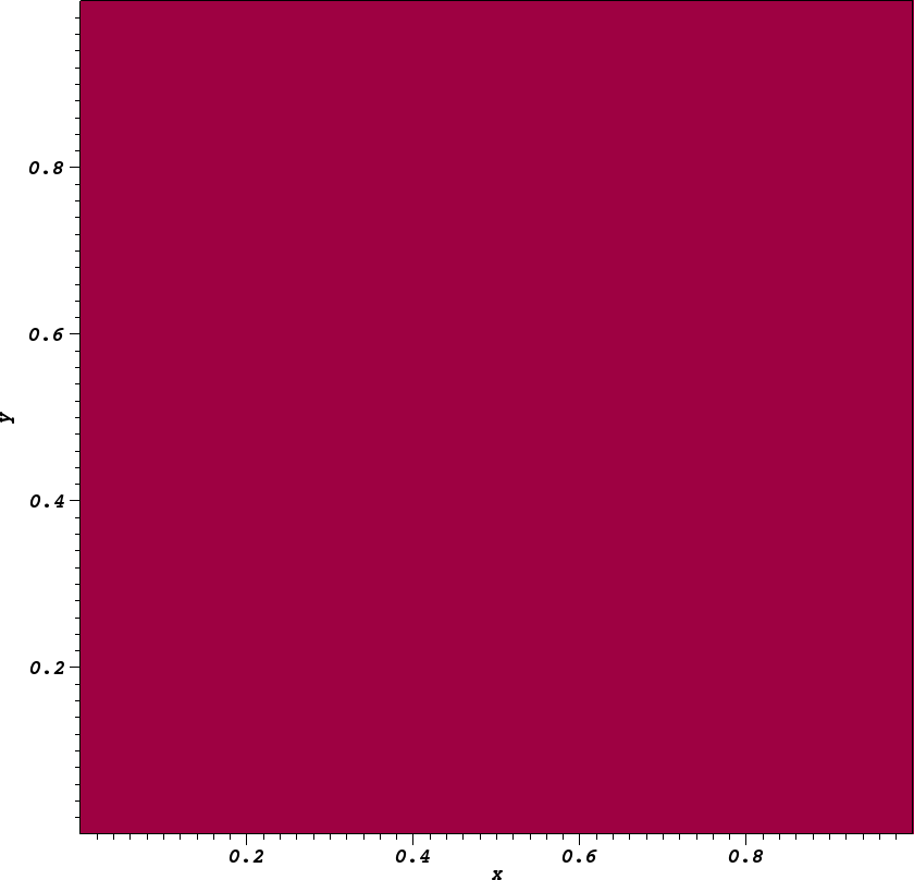
(a) Compatible flow-transport discretization.

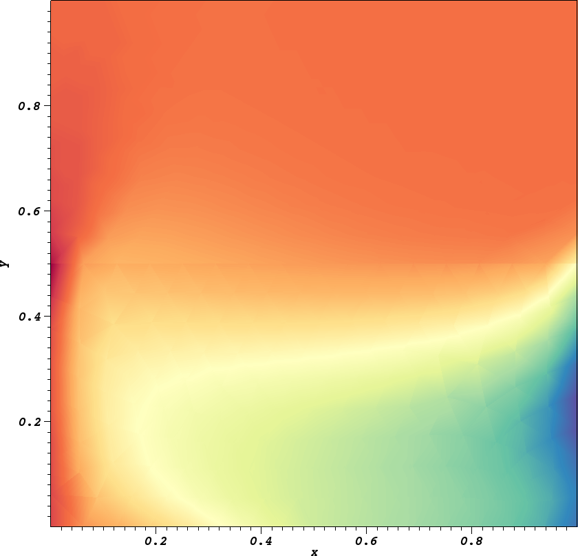
(b) Incompatible flow-transport discretization.

Figure 1: Test case from section 7.2. The solution to the transport equation at $t=1$. Left: the solution $c=1$ is approximated up to machine precision using the compatible EDG-HDG discretization. Right: an incompatible flow-transport discretization cannot preserve the constant solution $c=1$. Here $c_{h}\in[0.99927,1.00019]$.

7.3 Contaminant transport

We finally consider a simulation of coupled surface/subsurface flow and contaminant transport. This test case is similar to that proposed in [40, Example 7.2].

For the Stokes–Darcy problem we consider the same setup as in [9, Section 6.2]; we consider the unit square domain $\Omega=(0,1)^{2}$ which is divided into a Stokes region $\Omega^{s}=(0,1)\times(0.5,1)$ that represents a lake or a river, and a Darcy region $\Omega^{d}=\Omega\backslash\Omega^{s}$ representing an aquifer. The domain is divided into $14\,900$ simplicial elements. The mesh is such that $\mathcal{T}^{s}$ is an exact triangulation of $\Omega^{s}$, $\mathcal{T}^{d}$ is an exact triangulation of $\Omega^{d}$, and element boundaries match on the interface $\Omega^{s}\cap\Omega^{d}$. We use a time step of $\Delta t=10^{-3}$ and set $\ell=k-1=2$.

Let the boundary of the Stokes region be partitioned as $\Gamma^{s}=\Gamma^{s}_{1}\cup\Gamma_{2}^{s}\cup\Gamma_{3}^{s}$ where $\Gamma^{s}_{1}\mathrel{\mathop{\mathchar 58\relax}}=\mathinner{\{x\in\Gamma^{s}\ \mathrel{\mathop{\mathchar 58\relax}}\ x_{1}=0\}}$, $\Gamma^{s}_{2}\mathrel{\mathop{\mathchar 58\relax}}=\mathinner{\{x\in\Gamma^{s}\ \mathrel{\mathop{\mathchar 58\relax}}\ x_{1}=1\}}$ and $\Gamma^{s}_{3}\mathrel{\mathop{\mathchar 58\relax}}=\mathinner{\{x\in\Gamma^{s}\ \mathrel{\mathop{\mathchar 58\relax}}\ x_{2}=1\}}$. Similarly, let $\Gamma^{d}=\Gamma^{d}_{1}\cup\Gamma_{2}^{d}$ where $\Gamma^{d}_{1}\mathrel{\mathop{\mathchar 58\relax}}=\mathinner{\{x\in\Gamma^{d}\ \mathrel{\mathop{\mathchar 58\relax}}\ x_{1}=0\ \text{or}\ x_{1}=1\}}$ and $\Gamma^{d}_{2}\mathrel{\mathop{\mathchar 58\relax}}=\mathinner{\{x\in\Gamma^{d}\ \mathrel{\mathop{\mathchar 58\relax}}\ x_{2}=0\}}$. We impose the following boundary conditions:

$$u =(x_{2}(3/2-x_{2})/5,0) \text{on}\ \Gamma_{1}^{s},$$

$$\mathinner{\left(-2\mu\varepsilon(u)+p\mathbb{I}\right)}n =0 \text{on}\ \Gamma_{2}^{s},$$

$$u\cdot n =0 \text{on}\ \Gamma_{3}^{s},$$

$$\mathinner{\left(-2\mu\varepsilon(u)+p\mathbb{I}\right)}^{t} =0 \text{on}\ \Gamma_{3}^{s},$$

$$u\cdot n =0 \text{on}\ \Gamma_{1}^{d},$$

$$p =-0.05 \text{on}\ \Gamma_{2}^{d}.$$

We set the permeability to

$$\kappa(x)=700(1+0.5(\sin(10\pi x_{1})\cos(20\pi x_{2}^{2})+\cos^{2}(6.4\pi x_{1})\sin(9.2\pi x_{2})))+100.$$

Other parameters in eqs. 1 and 2 are set as $\mu=0.1$, $\alpha=0.5$, $f^{s}=0$, and $f^{d}=0$.

For the transport equation eq. 3 the diffusion tensor is set to

$$D(u_{h})=\begin{cases}\delta I,&\text{ in }\Omega^{s},\\ \phi d_{m}\mathbb{I}+d_{l}|u_{h}|\mathbb{T}+d_{t}|u_{h}|(\mathbb{I}-\mathbb{T}),&\text{ in }\Omega^{d},\end{cases}$$

where $u_{h}$ is the velocity solution to eq. 5, $\delta>0$, $d_{l},d_{t}\geq 0$ are longitudinal and transverse dispersivities and $d_{m}>0$ is the molecular diffusivity, $\mathbb{I}$ denotes the identity matrix, $\mathbb{T}=u_{h}u_{h}^{T}/|u_{h}|^{2}$ and $u_{h}^{T}$ is the transpose of the vector $u_{h}$. This diffusion tensor satisfies eqs. 4a, 4b and 22 (assuming $d_{l}\geq d_{t}$, which is usually the case) and eq. 4c [18, 39]. In our numerical example, we choose $\delta=10^{-6}$, $\phi=1$ on $\Omega^{s}$ and $\phi=0.4$ on $\Omega^{d}$ and $d_{m}=d_{l}=d_{t}=10^{-5}$. The initial condition for the plume of contaminant is given by

$$c_{0}(x)=\begin{cases}0.95&\text{if}\ \sqrt{(x_{1}-0.2)^{2}+(x_{2}-0.7)^{2}}<0.1,\\ 0.05&\text{otherwise}.\end{cases}$$

In fig. 2 we show the permeability and the computed velocity field (which are identical to [9, Figure 2]). In fig. 3 we show the plume of contaminant spreading through the surface water region and penetrating into the porous medium. As observed also in [40, Example 7.2], the contaminant plume stays compact while in the surface water region but spreads out in the groundwater region due to the heterogeneity of the porous media.

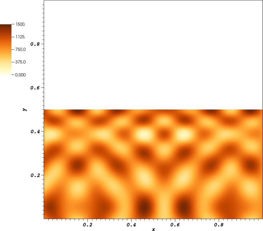
(a) The permeability.

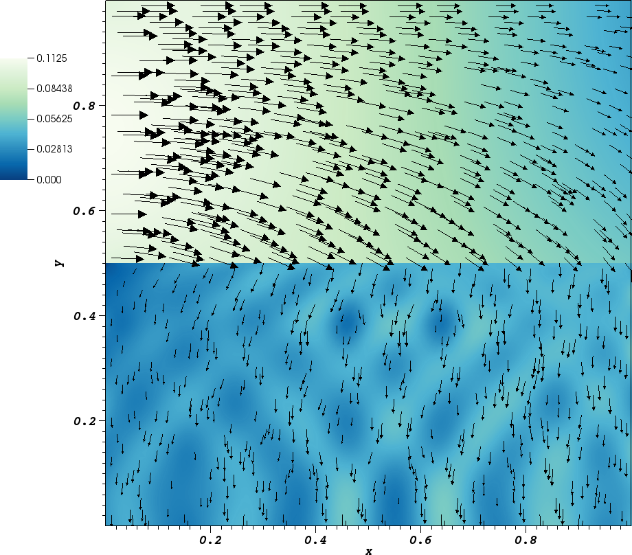
(b) The velocity field.

Figure 2: The permeability and computed velocity field for the test case described in section 7.3.

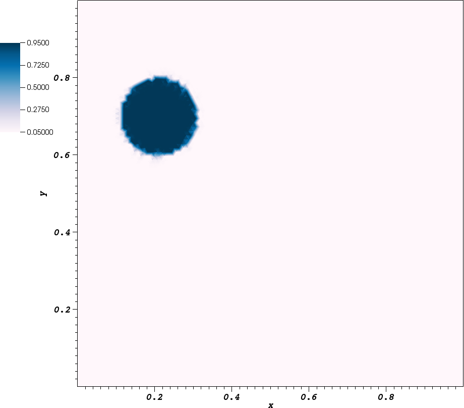
(a) The plume at $t=0$.

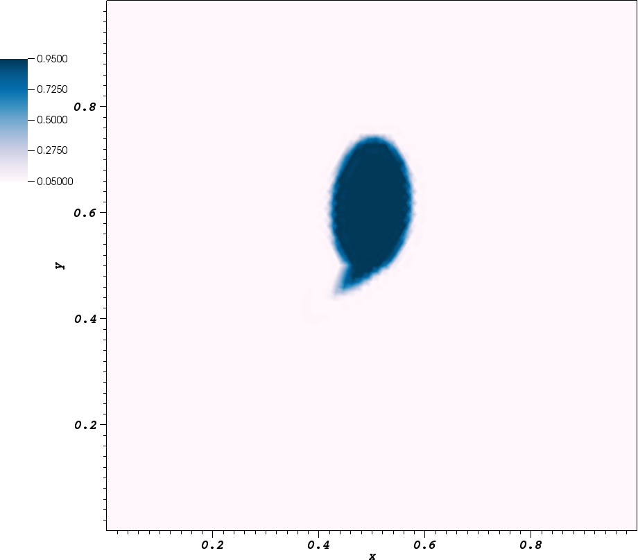
(b) The plume at $t=3.3$.

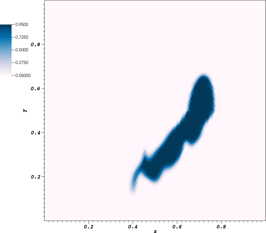
(c) The plume at $t=6.6$.

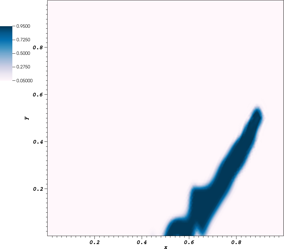
(d) The plume at $t=10$.

Figure 3: The plume of contaminant spreading through the surface water region and penetrating into the porous medium with snapshots at different instances in time. The test case is described in section 7.3.

8 Conclusions

We have analyzed a compatible embedded-hybridized discontinuous Galerkin discretization for the one-way coupling between Stokes–Darcy flow and transport and proved existence and uniqueness and optimal convergence rates for the discrete transport problem. These results complement our previous work in which we proved optimal and pressure-robust error estimates for the EDG-HDG discretization of the Stokes–Darcy system. We verified our theory by numerical examples. We furthermore demonstrated that an incompatible discretization of the coupled Stokes–Darcy and transport problem can result in small oscillations in the solution to the transport equation. This shows the importance of compatible discretizations for coupled flow and transport problems.

References

- Bainov and Simeonov [1992] D. D. Bainov and P. S. Simeonov. Integral inequalities and applications, volume 57 of Springer Series in Mathematics and Its Applications. Springer Netherlands, 1992.
- Beavers and Joseph [1967] G. S. Beavers and D. D. Joseph. Boundary conditions at a naturally impermeable wall. J. Fluid. Mech, 30(1):197–207, 1967. doi: 10.1017/S0022112067001375.
- Brenner and Scott [2008] S. C. Brenner and L. R. Scott. The Mathematical Theory of Finite Element Methods. Springer Series Texts in Applied Mathematics. Springer Science+Business Media, LLC, third edition, 2008.
- Brooks and Hughes [1982] A. N. Brooks and T. J. R. Hughes. Streamline upwind Petrov–Galerkin formulations for convection dominated flows with particular emphasis on the incompressible Navier–Stokes equation. Comput. Meth. Appl. Mech. Engrg., 32(1–3):199–259, 1982. doi: 10.1016/0045-7825(82)90071-8.
- Burman and Hansbo [2005] E. Burman and P. Hansbo. Stabilized Crouzeix–Raviart element for the Darcy–Stokes problem. Numer. Meth. Part. D. E., 21(5):986–97, 2005. doi: 10.1002/num.20076.
- Camano et al. [2015] J. Camano, G. N. Gatica, R. Oyarzúa, R. Ruiz-Baier, and P. Venegas. New fully-mixed finite element methods for the Stokes–Darcy coupling. Comput. Method. Appl. M., 295:362–395, 2015. doi: 10.1016/j.cma.2015.07.007.
- Cao et al. [2010] Y. Cao, M. Gunzburger, X. Hu, F. Hua, X. Wang, and W. Zhao. Finite element approximations for Stokes–Darcy flow with Beavers–Joseph interface conditions. SIAM J. Numer. Anal., 47(6):4239–4256, 2010. doi: 10.1137/080731542.
- Çeşmelioğlu and Rivière [2009] A. Çeşmelioğlu and B. Rivière. Primal discontinuous Galerkin methods for time-dependent coupled surface and subsurface flow. J. Sci. Comput., 40(1):115–140, 2009. doi: 10.1007/s10915-009-9274-4.
- Cesmelioglu et al. [2020] A. Cesmelioglu, S. Rhebergen, and G. N. Wells. An embedded-hybridized discontinuous Galerkin method for the coupled Stokes–Darcy system. J. Comput. Appl. Math, 367, 2020. doi: 10.1016/j.cam.2019.112476.
- Ciarlet [2002] P. Ciarlet. The Finite Element Method for Elliptic Problems. Society for Industrial and Applied Mathematics, 2002. doi: 10.1137/1.9780898719208.
- Cockburn and Shu [1998] B. Cockburn and C.-W. Shu. The local discontinuous Galerkin finite element method for time-dependent convection–diffusion systems. SIAM J. Numer. Anal., 35(6):2440–2463, 1998. doi: 10.1137/S0036142997316712.
- Cockburn et al. [2009] B. Cockburn, J. Gopalakrishnan, and R. Lazarov. Unified hybridization of discontinuous Galerkin, mixed, and continuous Galerkin methods for second order elliptic problems. SIAM J. Numer. Anal., 47(2):1319–1365, 2009. doi: 10.1137/070706616.
- Correa and Loula [2009] M. R. Correa and A. F. D. Loula. A unified mixed formulation naturally coupling Stokes and Darcy flows. Comput. Methods Appl. Mech. Engrg., 198(33-36):2710–2722, 2009. doi: 10.1016/j.cma.2009.03.016.
- D’Angelo and Zunino [2011] C. D’Angelo and P. Zunino. Robust numerical approximation of coupled Stokes’ and Darcy’s flows applied to vascular hemodynamics and biochemical transport. ESAIM: M2AN, 45(3):447–476, 2011. doi: 10.1051/m2an/2010062.
- Dawson and Proft [2001] C. Dawson and J. Proft. A priori error estimates for interior penalty versions of the local discontinuous Galerkin method applied to transport equations. Numer. Meth. Part. D. E., 17(6):545–564, 2001. doi: 10.1002/num.1026.
- Dawson et al. [2004] C. Dawson, S. Sun, and M. F. Wheeler. Compatible algorithms for coupled flow and transport. Comput. Methods Appl. Mech. Engrg., 193:2565–2580, 2004. doi: 10.1016/j.cma.2003.12.059.
- Discacciati et al. [2002] M. Discacciati, E. Miglio, and A. Quarteroni. Mathematical and numerical models for coupling surface and groundwater flows. Appl. Numer. Math., 43(1):57–74, 2002. doi: 10.1016/S0168-9274(02)00125-3.
- Douglas Jr. et al. [1983] J. Douglas Jr., R. E. Ewing, and M. F. Wheeler. A time-discretization procedure for a mixed finite element approximation of miscible displacement in porous media. RAIRO. Anal. numér., 17(3):249–265, 1983. doi: 10.1051/m2an/1983170302491.
- Egger and Waluga [2013] H. Egger and C. Waluga. A hybrid discontinuous Galerkin method for Darcy–Stokes problems. In R. Bank, M. Holst, O. Widlund, and J. Xu, editors, Domain Decomposition Methods in Science and Engineering XX, pages 663–670. Springer Berlin Heidelberg, 2013. doi: 10.1007/978-3-642-35275-1˙79.
- Fu and Lehrenfeld [2018] G. Fu and C. Lehrenfeld. A strongly conservative hybrid DG/mixed FEM for the coupling of Stokes and Darcy flow. J. Sci. Comput., 77, 2018. doi: 10.1007/s10915-018-0691-0.
- Gatica and Sequeira [2017] G. N. Gatica and F. A. Sequeira. Analysis of the HDG method for the Stokes–Darcy coupling. Numer. Meth. Part. D. E., 33(3):885–917, 2017. doi: 10.1002/num.22128.
- Gatica et al. [2009] G. N. Gatica, S. Meddahi, and R. Oyarzúa. A conforming mixed finite-element method for the coupling of fluid flow with porous media flow. IMA J. Numer. Anal., 29:86–108, 2009. doi: 10.1093/imanum/drm049.
- Girault and Rivière [2009] V. Girault and B. Rivière. DG approximation of coupled Navier–Stokes and Darcy equations by Beaver–Joseph–Saffman interface condition. SIAM J. Numer. Anal., 47(3):2052–2089, 2009. doi: 10.1137/070686081.
- Girault et al. [2014] V. Girault, G. Kanschat, and B. Rivière. Error analysis for a monolithic discretization of coupled Darcy and Stokes problems. J. Numer. Math., 22(2):109–142, 2014. doi: 10.1515/jnma-2014-0005.
- Houston et al. [2002] P. Houston, C. Schwab, and E. Süli. Discontinuous hp-finite element methods for advection-diffusion-reaction problems. SIAM J. Numer. Anal., 39(6):2133–2163, 2002. doi: 10.1137/S0036142900374111.
- Hughes and Wells [2005] T. J. R. Hughes and G. N. Wells. Conservation properties for the Galerkin and stabilised forms of the advection-diffusion and incompressible Navier–Stokes equations. Comput. Methods Appl. Mech. and Engrg., 194(9–11):1141–1159, 2005. doi: 10.1016/j.cma.2004.06.034.
- Igreja and Loula [2018] I. Igreja and A. F. D. Loula. A stabilized hybrid mixed dgfem naturally coupling stokes–darcy flows. Comput. Methods Appl. Mech. and Engrg., 339:739–768, 2018. doi: 10.1016/j.cma.2018.05.026.
- Layton et al. [2002] W. Layton, F. Schieweck, and I. Yotov. Coupling fluid flow with porous media flow. SIAM J. Numer. Anal., 40(6):2195–2218, 2002. doi: 10.1137/S0036142901392766.
- Lipnikov et al. [2014] K. Lipnikov, D. Vassilev, and I. Yotov. Discontinuous Galerkin and mimetic finite difference methods for coupled Stokes–Darcy flows on polygonal and polyhedral grids. Numer. Math., 126(2):321–360, 2014. doi: 10.1007/s00211-013-0563-3.
- Márquez et al. [2015] A. Márquez, S. Meddahi, and F.-J. Sayas. Strong coupling of finite element methods for the Stokes–Darcy problem. IMA J. Numer. Anal., 35(2):969–988, 2015. doi: 10.1093/imanum/dru023.
- Nguyen et al. [2009] N. C. Nguyen, J. Peraire, and B. Cockburn. An implicit high-order hybridizable discontinuous Galerkin method for linear convection-diffusion equations. J. Comput. Phys., 228(9):3232–3254, 2009. doi: 10.1016/j.jcp.2009.01.030.
- Pietro and Ern [2012] D. A. D. Pietro and A. Ern. Mathematical Aspects of Discontinuous Galerkin Methods, volume 69 of Mathématiques et Applications. Springer–Verlag Berlin Heidelberg, 2012.
- Rhebergen and Wells [2020] S. Rhebergen and G. N. Wells. An embedded-hybridized discontinuous Galerkin finite element method for the Stokes equations. Comput. Methods Appl. Mech. Engrg., 358, 2020. doi: 10.1016/j.cma.2019.112619.
- Rivière [2005] B. Rivière. Analysis of a discontinuous finite element method for the coupled Stokes and Darcy problems. J. Sci. Comput., 22(1):479–500, 2005. doi: 10.1007/s10915-004-4147-3.
- Riviere [2014] B. Riviere. Discontinuous finite element methods for coupled surface–subsurface flow and transport problems. In X. Feng, O. Karakashian, and Y. Xing, editors, Recent Developments in Discontinuous Galerkin Finite Element Methods for Partial Differential Equations: 2012 John H. Barrett Memorial Lectures, pages 259–279, Cham, 2014. Springer International Publishing. doi: 10.1007/978-3-319-01818-8˙11.
- Rivière and Yotov [2005] B. Rivière and I. Yotov. Locally conservative coupling of Stokes and Darcy flows. SIAM J. Numer. Anal., 42(5):1959–1977, 2005. doi: 10.1137/S0036142903427640.
- Saffman [1971] P. Saffman. On the boundary condition at the surface of a porous media. Stud. Appl. Math., 50:292–315, 1971.
- Schöberl [2014] J. Schöberl. C++11 implementation of finite elements in NGSolve. Technical Report ASC Report 30/2014, Institute for Analysis and Scientific Computing, Vienna University of Technology, 2014. URL http://www.asc.tuwien.ac.at/~schoeberl/wiki/publications/ngs-cpp11.pdf.
- Sun et al. [2002] S. Sun, B. Rivière, and M. F. Wheeler. A combined mixed finite element and discontinuous Galerkin method for miscible displacement problem in porous media. In Recent Progress in Computational and Applied PDES, pages 323–351, Boston, MA, 2002. Springer US.
- Vassilev and Yotov [2009] D. Vassilev and I. Yotov. Coupling Stokes–Darcy flow with transport. SIAM J. Sci. Comput., 31(5):3661–3684, 2009. doi: 10.1137/080732146.
- Wells [2011] G. N. Wells. Analysis of an interface stabilized finite element method: the advection-diffusion-reaction equation. SIAM J. Numer. Anal., 49(1):87–109, 2011. doi: 10.1137/090775464.