Large genus asymptotic geometry of random square-tiled surfaces and of random multicurves

Abstract.

We study the combinatorial geometry of a random closed multicurve on a surface of large genus $g$ and of a random square-tiled surface of large genus $g$. We prove that primitive components $\gamma_{1},\dots,\gamma_{k}$ of a random multicurve $m_{1}\gamma_{1}+\dots+m_{k}\gamma_{k}$ represent linearly independent homology cycles with asymptotic probability $1$ and that all its weights $m_{i}$ are equal to $1$ with asymptotic probability $\sqrt{2}/2$. We prove analogous properties for random square-tiled surfaces. In particular, we show that all conical singularities of a random square-tiled surface belong to the same leaf of the horizontal foliation and to the same leaf of the vertical foliation with asymptotic probability $1$.

We show that the number of components of a random multicurve and the number of maximal horizontal cylinders of a random square-tiled surface of genus $g$ are both very well-approximated by the number of cycles of a random permutation for an explicit non-uniform measure on the symmetric group of $3g-3$ elements. In particular, we prove that the expected value of these quantities is asymptotically equivalent to $(\log(6g-6)+\gamma)/2+\log 2$.

These results are based on our formula for the Masur–Veech volume $\operatorname{Vol}\mathcal{Q}_{g}$ of the moduli space of holomorphic quadratic differentials combined with deep large genus asymptotic analysis of this formula performed by A. Aggarwal and with the uniform asymptotic formula for intersection numbers of $\psi$-classes on $\overline{\mathcal{M}}_{g,n}$ for large $g$ proved by A. Aggarwal in 2020.

1. Introduction and statements of main results

We aim to study random multicurves on surfaces of large genus $g$. Before proceeding to the statements of our main results we consider the classical setting of random integers and of random permutations which allow to set up the concept of a random compound object. For more information on the probabilistic analysis of decomposition of combinatorial objects into elementary components we recommend the monograph of R. Arratia, A. D. Barbour, S. Tavaré [ABaT03]. An enlightening introduction can be found in the blog post of T. Tao [Tao13].

Prime decomposition of a random integer. The Prime Number Theorem states that an integer number $n$ taken randomly in a large interval $[1,N]$ is prime with asymptotic probability $\frac{\log N}{N}$. Denote by $\omega(n)$ the number of prime divisors of an integer $n$ counted without multiplicities. In other words, if $n$ has prime decomposition $n=p_{1}^{m_{1}}\dots p_{k}^{m_{k}}$, let $\omega(n)=k$. By the Erdős–Kac theorem [EK39], the centered and rescaled distribution prescribed by the counting function $\omega(n)$ tends to the normal distribution:

(1.1) $$\lim_{N\to+\infty}\frac{1}{N}\operatorname{card}\left\{n\leq N\,\Big{|}\,\frac{\omega(n)-\log\log N}{\sqrt{\log\log N}}\leq x\right\}=\frac{1}{\sqrt{2\pi}}\int_{-\infty}^{x}e^{-\tfrac{t^{2}}{2}}dt\,.$$

The subsequent papers of A. Rényi and P. Turán [RT58], and of A. Selberg [Se54] describe the rate of convergence.

Cycle decomposition of a uniform random permutation. Denote by ${\mathrm{K}}_{n}(\sigma)$ the number of disjoint cycles in the cycle decomposition of a permutation $\sigma$ in the symmetric group $S_{n}$. Consider the uniform probability measure on $S_{n}$. A random permutation $\sigma$ of $n$ elements has exactly $k$ cycles in its cyclic decomposition with probability ${\mathbb{P}}\big{(}{\mathrm{K}}_{n}(\sigma)=k\big{)}=\frac{s(n,k)}{n!}$, where $s(n,k)$ is the unsigned Stirling number of the first kind. It is immediate to see that ${\mathbb{P}}\big{(}{\mathrm{K}}_{n}(\sigma)=1\big{)}=\tfrac{1}{n}$. V. L. Goncharov proved in [Gon44] the following expansions for the expected value and for the variance of ${\mathrm{K}}_{n}$ as $n\to+\infty$:

(1.2) $${\mathbb{E}}({\mathrm{K}}_{n})=\log n+\gamma+o(1)\,,\qquad{\mathbb{V}}({\mathrm{K}}_{n})=\log n+\gamma-\zeta(2)+o(1)\,,$$

as well as the following central limit theorem

(1.3) $$\lim_{n\to+\infty}\frac{1}{n!}\operatorname{card}\left\{\sigma\in S_{n}\,\Big{|}\,\frac{{\mathrm{K}}_{n}(\sigma)-\log n}{\sqrt{\log n}}\leq x\right\}=\frac{1}{\sqrt{2\pi}}\int_{-\infty}^{x}e^{-\tfrac{t^{2}}{2}}dt\,.$$

As can be seen in (1.2) and in (1.3), the number of cycles in the cycle decomposition of a random permutation is of the order of $\log n$, so cycles are “rare events”. In such situation one expects the distribution to be close to a Poisson distribution. Recall that the Poisson distribution with parameter $\lambda$ is

(1.4) $$\mathrm{Poi}_{\lambda}(k)=e^{-\lambda}\ \frac{\lambda^{k}}{k!}\,,\qquad\text{where }k=0,1,2,\dots$$

H. Hwang proved in [Hw94] that the distribution of the random variable ${\mathrm{K}}_{n}$ is approximated by the Poisson distribution $\mathrm{Poi}_{\log n}$ in a very strong sense, which can be formalized as “mod-Poisson converges with parameter $\log n$ and limiting function $1/\Gamma(t)$”, using the terminology of E. Kowalski and A. Nikeghbali [KoNi10]. We discuss the notion of mod-Poisson convergence in Section 3.2. We emphasize that such approximation is much stronger than the central limit theorem.

The result of H. Hwang [Hw95] (representing a particular case of results in [Hw94, Chapter 5]) implies, that for large $n$ and for any positive $x$, the distribution of the number of cycles is uniformly well-approximated in a neighborhood of $x\log n$ by the Poisson distribution with parameter $\log n+\operatorname{a}(x)$, where the explicit correctional constant term $\operatorname{a}(x)$ is completely determined by the limiting function and does not depend on $n$. Namely, for any $x>0$ we have uniformly in $0\leq k\leq x\log n$

(1.5) $${\mathbb{P}}\big{(}{\mathrm{K}}_{n}=k+1\big{)}=\frac{(\log n)^{k}}{n\cdot k!}\left(\frac{1}{\Gamma(1+\frac{k}{\log n})}+O\left(\frac{k}{(\log n)^{2}}\right)\right).$$

Shape of a random multicurve on a surface of fixed genus. Consider a smooth oriented closed surface $S$ of genus $g$. A multicurve $\gamma=\sum m_{i}\gamma_{i}$ (as the one in the picture by D. Calegari from [Ca07] presented in Figure 1) is a formal weighted sum of curves $\gamma_{i}$ with strictly positive integer weights $m_{i}$ where $\gamma_{1},\dots,\gamma_{k}$ is a collection of non-contractible simple curves on $S$ that are pairwise non-isotopic. Following the usual convention, we do not distinguish between the free homotopy class of a multicurve and the multicurve itself.

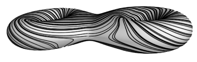
Figure 1. Simple closed multicurve on a surface of genus two

Every multicurve $\gamma=\sum m_{i}\gamma_{i}$ defines a reduced multicurve $\gamma_{\mathit{reduced}}=\sum\gamma_{i}$. Note that the number of reduced multicurves on a surface of a fixed genus $g$ considered up to the action of the mapping class group $\operatorname{Mod}_{g}$ is finite. We say that two multicurves have the same topological type if they belong to the same orbit of $\operatorname{Mod}_{g}$. For example, a simple closed curve has one of the following topological types: either it is non-separating, or it separates the surface into subsurfaces of genera $g^{\prime}$ and $g-g^{\prime}$ for some $1\leq g^{\prime}\leq g/2$.

Multicurves on a closed surface of genus $g$ (considered up to free homotopy) are parameterized by integer points $\mathcal{ML}_{g}({\mathbb{Z}})$ in the space of measured laminations $\mathcal{ML}_{g}$ introduced by W. Thurston [Th79]. Any hyperbolic metric on $S$ provides a length function $\ell$ that associates to a closed curve $\gamma$ the length $\ell(\gamma)$ of its unique geodesic representative. The length function $\ell$ extends to multicurves as $\ell(\gamma)=m_{1}\ell(\gamma_{1})+\ldots+m_{k}\ell(\gamma_{k})$. Fixing some upper bound $L$ for the length of a multicurve, one can consider the finite set of multicurves of length at most $L$ on $S$ with respect to the length function $\ell$. See also the paper of M. Mirzakhani [Mi04] and works of V. Erlandsson, H. Parlier, K. Rafi and J. Souto [RaSo19], [ErPaSo20] and [ErSo20] for alternative ways to measure the length of a multicurve.

Choosing the uniform measure on all integral multicurves of length at most $L$ and letting $L$ tend to infinity we define a “random multicurve” on a surface of fixed genus $g$ in the same manner as we considered “random integers”, see Section 2.4 for details. We emphasize that studying asymptotic statistical geometry of multicurves as the bound $L$ tends to infinity we always keep the genus $g$, considered as a parameter, fixed. One can ask, for example, what is the probability that a random simple closed curve separates the surface of genus $g$ in two components? Or, more generally, what is the probability that the reduced multicurve $\gamma_{\mathit{reduced}}$ associated to a random multicurve $\gamma$ separates the surface of genus $g$ into several components? With what probability a random multicurve $m_{1}\gamma_{1}+m_{2}\gamma_{2}+\dots+m_{k}\gamma_{k}$ has $k=1,2,\dots,3g-3$ primitive connected components $\gamma_{1},\dots,\gamma_{k}$? What are the typical weights $m_{1},\dots,m_{k}$?

A beautiful answer to all these questions was found by M. Mirzakhani in [Mi08a]. She expressed the frequency of multicurves of any fixed topological type in terms of the intersection numbers $\int_{\overline{\mathcal{M}}_{g^{\prime},n^{\prime}}}\psi_{1}^{d_{1}}\dots\psi_{n^{\prime}}^{d_{n^{\prime}}}$, where $2g^{\prime}+n^{\prime}\leq 2g$. (These intersection numbers are also called correlators of Witten’s two dimensional topological gravity). For small genera $g$ the formula of M. Mirzakhani provides explicit rational values for the quantities discussed above. For example, the reduced multicurve associated to a random multicurve on a surface of genus $2$ without cusps as in Figure 1 separates the surface with probability $\tfrac{67}{315}$ and has $1$, $2$ or $3$ components with probabilities $\tfrac{7}{27},\tfrac{5}{9},\tfrac{5}{27}$ respectively.

The formulae of Mirzakhani are applicable to surfaces of any genera. The exact values of the intersection numbers can be computed through Witten–Kontsevich theory [Wi91], [Kon92]. However, despite the fact that these intersection numbers were extensively studied, there were no uniform estimates for Witten correlators for large $g$ till the recent results of A. Aggarwal [Ag20b]. This is one of the reasons why the following question remained open.

Question 1.

What shape has a random multicurve on a surface of large genus?

The current paper aims to answer this question to some extent. Denote by $K_{g}(\gamma)$ the number of components $k$ of the multicurve $\gamma=\sum_{i=1}^{k}m_{i}\gamma_{i}$ counted without multiplicities.

Theorem 1.1.

Consider a random multicurve $\gamma=\sum_{i=1}^{k}m_{i}\gamma_{i}$ on a surface $S$ of genus $g$. Let $\gamma_{\mathit{reduced}}=\gamma_{1}+\dots+\gamma_{k}$ be the underlying reduced multicurve. The following asymptotic properties hold as $g\to+\infty$.

• The multicurve $\gamma_{\mathit{reduced}}$ does not separate the surface (i.e. $S-\sqcup\gamma_{i}$ is connected) with probability which tends to 1.

• The probability that a random multicurve $\gamma=\sum_{i=1}^{k}m_{i}\gamma_{i}$ is primitive (i.e. that $m_{1}=m_{2}=\dots=1$) tends to $\frac{\sqrt{2}}{2}$.

• For any sequence of positive integers $k_{g}$ with $k_{g}=o(\log g)$ the probability that a random multicurve $\gamma=\sum_{i=1}^{k_{g}}m_{i}\gamma_{i}$ is primitive (i.e. that $m_{1}=\dots=m_{k_{g}}=1$) tends to $1$ as $g\to+\infty$.

There is no contradiction between parts (b) and (c) of the above Theorem since in (c) we consider only those random multicurves for which the underlying primitive multicurve has an imposed number $k_{g}$ of components, while in (b) we consider all multicurves. In other words, in part (c) we consider the conditional probability. Part (b) of the above Theorem admits the following generalization.

Theorem 1.2.

For any positive integer $m$, the probability that all weights $m_{i}$ of a random multicurve $\gamma=m_{1}\gamma_{1}+m_{2}\gamma_{2}+\dots$ on a surface of genus $g$ are bounded by a positive integer $m$ (i.e. that $m_{1}\leq m,m_{2}\leq m,\dots$) tends to $\sqrt{\frac{m}{m+1}}$ as $g\to+\infty$.

We describe the probability distribution of the random variable $K_{g}(\gamma)$ later in this section. However, to follow comparison with prime decomposition of random integers and with cycle decomposition of random permutations we present here the central limit theorem stated for random multicurves.

Theorem 1.3.

Choose a non-separating simple closed curve $\rho_{g}$ on a surface of genus $g$. Denote by $\iota(\rho_{g},\gamma)$ the geometric intersection number of $\rho_{g}$ and $\gamma$. The centered and rescaled distribution defined by the counting function $K_{g}(\gamma)$ tends to the normal distribution:

$$\lim_{g\to+\infty}\sqrt{\frac{3\pi g}{2}}\cdot 12g\cdot(4g-4)!\cdot\left(\frac{9}{8}\right)^{2g-2}\\ \lim_{N\to+\infty}\frac{1}{N^{6g-6}}\operatorname{card}\Bigg{(}\bigg{\{}\gamma\in\mathcal{ML}_{g}({\mathbb{Z}})\,\bigg{|}\,\iota(\rho_{g},\gamma)\leq N\quad\text{and}\\ \frac{K_{g}(\gamma)-\frac{\log g}{2}}{\sqrt{\frac{\log g}{2}}}\leq x\bigg{\}}/\operatorname{Stab}(\rho_{g})\Bigg{)}=\frac{1}{\sqrt{2\pi}}\int_{-\infty}^{x}e^{-\tfrac{t^{2}}{2}}dt\,.$$

Here $\operatorname{Stab}(\rho_{g})\subset\operatorname{Mod}_{g}$ is the stabilizer of the simple closed curve $\rho_{g}$ in the mapping class group $\operatorname{Mod}_{g}$.

In plain words, the above theorems say that the components $\gamma_{1},\dots,\gamma_{k}$ of a random multicurve $\gamma=\sum_{i=1}^{k}m_{i}\gamma_{i}$ on a surface of large genus $g$ have all chances to go around $k$ independent handles, where $k$ is close to $\frac{1}{2}\log g$, and that with a high probability all the weights $m_{i}$ of a random multicurve are uniformly small. In particular, with probability greater than $0.7$ a random multicurve is primitive, i.e. all the weights $m_{i}$ are equal to $1$.

Our description of the asymptotic geometry of random multicurves on surfaces of large genus and of random square-tiled surfaces of large genera relies on fundamental recent results [Ag20b] of A. Aggarwal, who proved, in particular, the large genus asymptotic formulae for the Masur–Veech volume $\operatorname{Vol}\mathcal{Q}_{g}$ and for the intersection numbers of $\psi$-classes on $\overline{\mathcal{M}}_{g,n}$, conjectured by the authors in [DGZZ19].

Random square-tiled surfaces of large genus. A square-tiled surface is a closed oriented quadrangulated surface (i.e. a surface built by gluing identical squares along their edges), such that the quadrangulation satisfies the following properties. Consider the flat metric on the surface induced by the flat metric on the squares. We assume that edges of the squares are identified by isometries, which implies that the induced flat metric is non-singular on the complement of the vertices of the squares. We require that the parallel transport of a vector $\vec{v}$ tangent to the surface along any closed path avoiding conical singularities brings the vector $\vec{v}$ either to itself or to $-\vec{v}$. In other words, we require that the holonomy group of the metric is ${\mathbb{Z}}/2{\mathbb{Z}}$ (compared to ${\mathbb{Z}}/4{\mathbb{Z}}$ for a general quadrangulation). This holonomy assumption implies that defining some edge to be “horizontal” or “vertical” we uniquely determine for each of the remaining edges, whether it is “horizontal” or “vertical”. Speaking of square-tiled surfaced we always assume that the choice of horizontal and vertical edges is done.

Our holonomy assumption implies that the number of squares adjacent to any vertex is even. In this article we restrict ourselves to consideration of square-tiled surfaces with no conical singularities of angle $\pi$. In other words, vertices adjacent to exactly two squares are not allowed. Square-tiled surfaces satisfying the above restrictions can be seen as integer points in the total space $\mathcal{Q}_{g}$ of the vector bundle of holomorphic quadratic differentials over the moduli space of complex curves $\mathcal{M}_{g}$.

A stronger restriction on the quadrangulation imposing trivial linear holonomy to the induced flat metric defines Abelian square-tiled surfaces; they correspond to integer points in the total space $\mathcal{H}_{g}$ of the vector bundle of holomorphic Abelian differentials over the moduli space of complex curves $\mathcal{M}_{g}$. The subset of square-tiled surfaces having prescribed linear holonomy and prescribed cone angle at each conical singularity corresponds to the set of integer points in the associated stratum in the moduli space of quadratic or Abelian differentials respectively.

A square-tiled surface admits a natural decomposition into maximal horizontal cylinders. For example, the square-tiled surface in the left picture of Figure 2 (which, for simplicity of illustration, contains conical points with cone angles $\pi$) has four maximal horizontal cylinders highlighted by different shades of grey. Two of these cylinders are composed of two horizontal bands of squares. Each of the remaining two cylinders is composed of a single horizontal band of squares.

For any positive integer $N$, the set $\mathcal{ST}{}_{g}(N)$ of square-tiled surfaces of genus $g$ having no singularities of angle $\pi$ and having at most $N$ squares in the tiling is finite. Choosing the uniform measure on the set $\mathcal{ST}{}_{g}(N)$ and letting the bound $N$ for the number of squares tend to infinity, we define a “random square-tiled surface” of fixed genus $g$ in the same manner as we considered “random multicurves” on a fixed surface, see Section 2.5 for details. We emphasize that studying asymptotic statistical geometry of square-tiled surfaces as the bound $N$ tends to infinity we always keep the genus $g$, considered as a parameter, fixed. One can study the decomposition of a random square-tiled surface into maximal horizontal cylinders in the same sense as we considered prime decomposition of random integers or cyclic decomposition of random permutations.

For each stratum in the moduli space of Abelian differentials, we computed in [DGZZ20b] the probability that a random square-tiled surface in this stratum has a single cylinder in its horizontal cylinder decomposition. This result can be seen as an analog of the Prime Number Theorem for square-tiled surfaces. In particular, using results [Ag20a] and [CMöSZa20] we proved that for strata of Abelian differentials corresponding to large genera, this probability is asymptotically $\frac{1}{d}$, where $d$ is the dimension of the stratum. However, more detailed description of statistics of square-tiled surfaces in individual strata of Abelian differentials is currently out of reach with the exception of several low-dimensional strata. Conjecturally, for any stratum of Abelian differentials of dimension $d$, the statistics of the number of maximal horizontal cylinders of a random square-tiled surface in the stratum becomes very well-approximated by the statistics of the number ${\mathrm{K}}_{n}(\sigma)$ of disjoint cycles in a random permutation of $d$ elements as $d\to+\infty$; see Section 6.2 for details.

In the current paper we address more general question.

Question 2.

What shape has a random square-tiled surface of large genus assuming that it does not have conical points of angle $\pi$?

Denote by $K_{g}(S)$ the number of maximal horizontal cylinders in the cylinder decomposition of a square-tiled surface $S$ of genus $g$.

Theorem 1.4.

A random square-tiled surface $S$ of genus $g$ with no conical singularities of angle $\pi$ has the following asymptotic properties as $g\to+\infty$.

• All conical singularities of $S$ are located at the same leaf of the horizontal foliation and at the same leaf of the vertical foliation with probability which tends to 1.

• The probability that each maximal horizontal cylinder of $S$ is composed of a single band of squares tends to $\frac{\sqrt{2}}{2}$.

• For any sequence of positive integers $k_{g}$ with $k_{g}=o(\log g)$ the probability that each maximal horizontal cylinder of a random $k_{g}$-cylinder square-tiled surface of genus $g$ is composed of a single band of squares tends to $1$ as the genus $g$ tends to $+\infty$.

Similarly to the case of multicurves, part (b) of the above Theorem admits the following generalization.

Theorem 1.5.

For any $m\in{\mathbb{N}}$, the probability that all maximal horizontal cylinders of a random square-tiled surface of genus $g$ have at most $m$ bands of squares tends to $\sqrt{\frac{m}{m+1}}$ as $g\to+\infty$.

We state now the central limit theorem for square-tiled surfaces.

Theorem 1.6.

The centered and rescaled distribution defined by the counting function $K_{g}(S)$ tends to the normal distribution as $g\to+\infty$:

$$\lim_{g\to+\infty}3\pi g\cdot\left(\frac{9}{8}\right)^{2g-2}\\ \lim_{N\to+\infty}\frac{1}{N^{6g-6}}\operatorname{card}\left\{S\in\mathcal{ST}{}_{g}(N)\,\bigg{|}\,\frac{k(S)-\tfrac{\log g}{2}}{\sqrt{\tfrac{\log g}{2}}}\leq x\right\}=\frac{1}{\sqrt{2\pi}}\int_{-\infty}^{x}e^{-\frac{t^{2}}{2}}dt\,.$$

Approach to the study of random multicurves and of random square-tiled surfaces of large genera: from $p_{g}(k)$ to $q_{g}(k)$. It is time to admit that the parallelism between Theorems 1.1–1.3 and respectively Theorems 1.4–1.6 is not accidental.

Recall that we denote by $K_{g}(\gamma)$ the number of components $k$ of the multicurve $\gamma=\sum_{i=1}^{k}m_{i}\gamma_{i}$ on a surface of genus $g$ counted without multiplicities and by $K_{g}(S)$ the number of maximal horizontal cylinders in the cylinder decomposition of a square-tiled surface $S$ of genus $g$. The following theorem is a direct corollary of Theorem 1.21 from Section 1.8 in [DGZZ19]. (For the sake of completeness we reproduce the original Theorem in Section 2.5 below.)

Theorem 1.7.

For any genus $g\geq 2$ and for any $k\in{\mathbb{N}}$, the probability $p_{g}(k)$ that a random multicurve $\gamma$ on a surface of genus $g$ has exactly $k$ components counted without multiplicities coincides with the probability that a random square-tiled surface $S$ of genus $g$ has exactly $k$ maximal horizontal cylinders:

(1.6) $$p_{g}(k)={\mathbb{P}}\big{(}K_{g}(\gamma)=k\big{)}={\mathbb{P}}\big{(}K_{g}(S)=k\big{)}\,.$$

In other words, $K_{g}(\gamma)$ and $K_{g}(S)$, considered as random variables, determine the same probability distribution $p_{g}(k)$, where $k=1,2,\dots,3g-3$.

The Theorem above shows that Questions 1 and 2 are, basically, equivalent. The description of the large genus asymptotic properties of the resulting probability distribution $p_{g}(k)$ can be seen as the main unified goal of the current paper.

The starting point of our approach to the study of the probability distribution $p_{g}(k)$ is the the formula for the Masur–Veech volume $\operatorname{Vol}\mathcal{Q}_{g}$ of the moduli space of holomorphic quadratic differentials derived in our recent paper [DGZZ19]. This formula represents $\operatorname{Vol}\mathcal{Q}_{g}$ as a finite sum of contributions of square-tiled surfaces of all possible topological types (Section 2.3 describes this in detail). However, the number of such topological types grows exponentially as genus grows. Moreover, the contribution of square-tiled surfaces of a fixed topological type to $\operatorname{Vol}\mathcal{Q}_{g}$ is expressed in terms of the intersection numbers of $\psi$-classes (Witten correlators) which are difficult to evaluate explicitly in large genera.

We conjectured in [DGZZ19] that in large genera, the dominant part of the contribution to $\operatorname{Vol}\mathcal{Q}_{g}$ comes from square-tiled surfaces having all conical singularities at the same horizontal level. The topological type (see Section 2.1 for the rigorous definition of the “topological type”) of such square-tiled surfaces is completely determined by the number $k$ of maximal horizontal cylinders which varies from $1$ to $g$. This conjecture suggested a strategy for overcoming the first difficulty, reducing the study of all immense variety of topological types of square-tiled surfaces to the study of $g$ explicit topological types. We also conjectured in [DGZZ19] that under certain assumptions on $g$ and $n$, the intersection numbers $\int_{\overline{\mathcal{M}}_{g,n}}\psi_{1}^{d_{1}}\dots\psi_{n}^{d_{n}}$ are uniformly well-approximated by an explicit closed expression in the variables $d_{1},\dots,d_{n}$, and that the error term becomes uniformly small with respect to all possible partitions $d_{1}+\dots+d_{n}=3g-3+n$ for large values of $g$. This conjecture suggested a plan for overcoming the second difficulty reducing analysis of volume contributions of square-tiled surfaces of $g$ distinguished topological types to analysis of closed expressions in multivariate harmonic sums. Such analysis led us, in particular, to the conjectural large genus asymptotics of the Masur–Veech volume $\operatorname{Vol}\mathcal{Q}_{g}$.

In terms of the probability distributions, we replace the original distribution $p_{g}(k)$ with an auxiliary probability distribution $q_{g}(k)$ in this approach. The distribution $q_{g}(k)$ describes the contributions of square-tiled surfaces of $g$ distinguished topological types (corresponding to the situation when all conical singularities are located at same horizontal layer and the surface has $k=1,\dots,g$ maximal horizontal cylinders), where, moreover, we replace the Witten correlators with the corresponding asymptotic expressions. The precise definition of $q_{g}(k)$ is given in Equation (3.17) in Section 3.1. Informally, our conditional asymptotic result in [DGZZ19] stated that for large genera $g$ the auxiliary distribution $q_{g}(k)$ well-approximates the original probability distribution $p_{g}(k)$ modulo the conjectures mentioned above.

Deep analysis of volume contributions of square-tiled surfaces of different topological types was performed by A. Aggarwal in [Ag20b]. Moreover, in the same paper A. Aggarwal established uniform asymptotic bounds for Witten correlators using elegant approach through biased random walk. In particular, he proved all conjectures from [DGZZ19] (in a stronger form) transforming conditional results from [DGZZ19] into unconditional statements.

In the current paper we follow the original approach, approximating the probability distribution $p_{g}(k)$ with a slight modification of the probability distribution $q_{g}(k)$ as described above. However, the fine asymptotic analysis of A. Aggarwal allows to state that $q_{g}(k)$ “well-approximates” $p_{g}(k)$ in much stronger sense than it was claimed in the original preprint  [DGZZ19]. Moreover, we realized that our “slight modification of the probability distribution $q_{g}(k)$” has combinatorial interpretation of independent interest and admits a detailed description based on technique developed by H. Hwang in [Hw94].

Having explained the scheme of our approach we can state now the main results concerning the probability distribution $p_{g}(k)$. We start with a formal definition of the “slight modification of the probability distribution $q_{g}(k)$” through random permutations. It plays an important role in the current paper.

Random non-uniform permutations and distribution $\boldsymbol{q_{n,\infty,1/2}}$. Let $\theta$ be a sequence $\{\theta_{k}\}_{k\geq 1}$ of non-negative real numbers. Given a permutation $\sigma\in S_{n}$ with cycle type $(1^{\mu_{1}}2^{\mu_{2}}\ldots n^{\mu_{n}})$, where $1\cdot\mu_{1}+2\cdot\mu_{2}+\dots+n\cdot\mu_{n}=n$, we define its weight $w_{\theta}(\sigma)$ by the following formula:

$$w_{\theta}(\sigma)=\theta_{1}^{\mu_{1}}\theta_{2}^{\mu_{2}}\cdots\theta_{n}^{\mu_{n}}.$$

To every collection of positive numbers $\theta=\{\theta_{k}\}_{k\geq 1}$, we associate a probability measure on the symmetric group $S_{n}$ by means of the weight function defined above:

(1.7) $${\mathbb{P}}_{\theta,n}(\sigma):=\frac{w_{\theta}(\sigma)}{n!\cdot W_{\theta,n}}\,,\quad\text{where}\qquad W_{\theta,n}:=\frac{1}{n!}\sum_{\sigma\in S_{n}}w_{\theta}(\sigma)\quad\text{and}\quad k\in{\mathbb{N}}\,.$$

Denote by ${\mathbb{P}}_{n,\infty,1/2}$ the non-uniform probability measure on the symmetric group $S_{n}$ associated to the collection of strictly positive numbers $\theta_{k}=\zeta(2k)/2$, where $k=1,2,\dots$ and $\zeta$ is the Riemann zeta function. Consider the random variable ${\mathrm{K}}_{n}(\sigma)$ on the symmetric group $S_{n}$, where the random permutation $\sigma$ corresponds to the law ${\mathbb{P}}_{n,\infty,1/2}$ and ${\mathrm{K}}_{n}(\sigma)$ is the number of disjoint cycles in the cycle decomposition of such random permutation $\sigma$. The random variable ${\mathrm{K}}_{n}(\sigma)$ takes integer values in the range $[1,n]$. We introduce the following notation:

(1.8) $$q_{n,\infty,1/2}(k)={\mathbb{P}}_{n,\infty,1/2}\big{(}{\mathrm{K}}_{3g-3}(\sigma)=k\big{)}$$

for the law of the random variable ${\mathrm{K}}_{n}(\sigma)$ with respect to the probability measure ${\mathbb{P}}_{n,\infty,1/2}$. We prove in Section 3 series of results which informally can be summarized by the following claim: the probability distribution $q_{3g-3,\infty,1/2}$ well-approximates the probability distribution $q_{g}$. We admit that the approximating distribution $q_{g}$ will be formally defined only later, namely, in Equation (3.17) in Section 3.1 and, strictly speaking, would not be used explicitly. The above claim explains, however, our interest for the probability distribution $q_{3g-3,\infty,1/2}$ which would be actually used for approximation. An important step of comparison of distributions $p_{g}$ and $q_{3g-3,\infty,1/2}$ is established in Lemma 3.6 stated and proved in Section 3.2. Theorems 1.8 and 1.10 below carry comprehensive information on the probability distribution $q_{3g-3,\infty,1/2}(k)={\mathbb{P}}_{3g-3,\infty,1/2}\big{(}{\mathrm{K}}_{3g-3}(\sigma)=k\big{)}$.

Theorem 1.8.

Let ${\mathbb{P}}_{n,\infty,1/2}$ be the probability distribution on $S_{n}$ associated to the collection $\theta_{k}=\zeta(2k)/2$. Then for all $t\in{\mathbb{C}}$ we have as $n\to+\infty$

(1.9) $${\mathbb{E}}_{n,\infty,1/2}\left(t^{{\mathrm{K}}_{n}}\right)=(2n)^{\tfrac{t-1}{2}}\cdot\frac{t\cdot\Gamma(\tfrac{3}{2})}{\Gamma(1+\tfrac{t}{2})}\ \left(1+O\left(\frac{1}{n}\right)\right)\,,$$

where the error term is uniform for $t$ in any compact subset of ${\mathbb{C}}$.

For any $\lambda>0$, let $u_{\lambda,1/2}(k)$ for $k\in{\mathbb{N}}$ be the coefficients of the following Taylor expansion

(1.10) $$e^{\lambda(t-1)}\cdot\displaystyle\frac{t\cdot\Gamma\left(\tfrac{3}{2}\right)}{\Gamma\left(1+\tfrac{t}{2}\right)}=\sum_{k\geq 1}u_{\lambda,1/2}(k)\cdot t^{k}$$

Recall that $\Gamma\left(\tfrac{3}{2}\right)=\frac{\Gamma\left(\tfrac{1}{2}\right)}{2}=\frac{\sqrt{\pi}}{2}$. We have

$$u_{\lambda,1/2}(k)=\sqrt{\pi}\cdot e^{-\lambda}\cdot\frac{1}{k!}\cdot\sum_{i=1}^{k}\binom{k}{i}\cdot\phi_{i}\cdot\left(\frac{1}{2}\right)^{i}\cdot\lambda^{k-i}\,.$$

where the $\phi_{j}$ are defined through the Taylor expansion

(1.11) $$\frac{t}{\Gamma(1+t)}=\frac{1}{\Gamma(t)}=\sum_{j=1}^{+\infty}\phi_{j}\cdot\frac{t^{j}}{j!}\,.$$

The first values are given by

$$\phi_{1}=1;\quad\phi_{2}=2\gamma;\quad\phi_{3}=3\big{(}\gamma^{2}-\zeta(2)\big{)}.$$

Theorem 1.8 has the following consequence.

Corollary 1.9.

Uniformly in $k\geq 1$ we have as $n\to\infty$

$$q_{n,\infty,1/2}(k)=u_{\lambda_{n},1/2}(k)+O\left(\frac{1}{n}\right)$$

where $\lambda_{n}=\frac{\log(2n)}{2}$.

Theorem 1.8 and its Corollary 1.9 are particular cases of Theorem 3.12 and Corollary 3.11 stated and proved in Section 3.3. We also illustrate the numerical aspects of this approximation in Section 6.1.

Theorem 1.10.

Let $\lambda_{n}=\log(2n)/2$. Then, for any $x>0$, we have uniformly in $0\leq k\leq x\lambda_{n}$ the following asymptotic behavior as $n\to+\infty$

(1.12) $$q_{n,\infty,1/2}(k+1)={\mathbb{P}}_{n,\infty,1/2}({\mathrm{K}}_{n}(\sigma)=k+1)=\\ =e^{-\lambda_{n}}\cdot\frac{(\lambda_{n})^{k}}{k!}\cdot\left(\frac{\sqrt{\pi}}{2\Gamma\left(1+\frac{k}{2\lambda_{n}}\right)}+O\left(\frac{k}{(\log n)^{2}}\right)\right)\,.$$

For any $x>1$ such that $x\lambda_{n}$ is an integer we have

(1.13) $$\sum_{k=x\lambda_{n}+1}^{n}q_{n,\infty,1/2}(k+1)={\mathbb{P}}_{n,\infty,1/2}\big{(}{\mathrm{K}}_{n}(\sigma)>x\lambda_{n}+1\big{)}=\\ =\frac{(2n)^{-\tfrac{x\log x-x+1}{2}}}{\sqrt{2\pi\lambda_{n}x}}\cdot\frac{x}{x-1}\cdot\left(\frac{\sqrt{\pi}}{2\Gamma\left(1+\frac{x}{2}\right)}+O\left(\frac{1}{\log n}\right)\right)\,,$$

where the error term is uniform over $x$ in compact subsets of $(1,+\infty)$. Similarly, for any $0<x<1$ such that $x\lambda_{n}$ is an integer we have

(1.14) $$\sum_{k=0}^{x\lambda_{n}}q_{n,\infty,1/2}(k+1)={\mathbb{P}}_{n,\infty,1/2}\big{(}{\mathrm{K}}_{n}(\sigma)\leq x\lambda_{n}+1\big{)}=\\ =\frac{(2n)^{-\tfrac{x\log x-x+1}{2}}}{\sqrt{2\pi\lambda_{n}x}}\cdot\frac{x}{1-x}\cdot\left(\frac{\sqrt{\pi}}{2\Gamma\left(1+\frac{x}{2}\right)}+O\left(\frac{1}{\log n}\right)\right)\,,$$

where the error term is uniform over $x$ in compact subsets of $(0,1)$.

Theorem 1.10 is a particular case of Corollary 3.17 stated and proved in Section 3.4. Note that for $x\not=1$, we have $x\log x-x+1>0$. Hence, Equations (1.13) and (1.14) provide explicit polynomial bounds in $n$ for the tails of the distribution.

Remark 1.11.

Let $\displaystyle G(x)=\frac{\sqrt{\pi}}{2\Gamma(1+\tfrac{x}{2})}$ and define

(1.15) $$\operatorname{a}(x)=\frac{\log G(x)}{x-1}.$$

Since $\log G(1)=0$, the function $\operatorname{a}(x)$ admits a continuous extension at $x=1$

$$\lim_{x\to 1}\operatorname{a}(x)=G^{\prime}(1)=\frac{\gamma}{2}+\log(2)-1\,,$$

where $\gamma$ is the Euler–Mascheroni constant. Now for any $x>0$, uniformly for $0\leq k\leq x\lambda_{n}$ we have

$$(\lambda_{n})^{k}\cdot G\left(\frac{k}{\lambda_{n}}\right)=e^{-\operatorname{a}\left(\frac{k}{\lambda_{n}}\right)}\left(\lambda_{n}+\operatorname{a}\left(\tfrac{k}{\lambda_{n}}\right)\right)^{k}\cdot\left(1+O\left(\frac{k}{\lambda_{n}^{2}}\right)\right)\,.$$

We can hence rewrite the right-hand side of (1.12): for any $x>0$ we have uniformly in $0\leq k\leq x\lambda_{n}$ the following asymptotic behavior as $n\to+\infty$

$$q_{n,\infty,1/2}(k+1)=e^{-\left(\lambda_{n}+\operatorname{a}\left(\frac{k}{\lambda_{n}}\right)\right)}\cdot\frac{\left(\lambda_{n}+\operatorname{a}\left(\tfrac{k}{\lambda_{n}}\right)\right)^{k}}{k!}\cdot\left(1+O\left(\frac{k}{(\log n)^{2}}\right)\right)\,.$$

In the latter expression, the right-hand side reads as the value of a Poisson random variable with parameter $\lambda_{n}+\operatorname{a}\left(\frac{k}{\lambda_{n}}\right)$.

The extended version of the above results as well as the closely related notion of mod-Poisson convergence are discussed in Section 3.2. The above theorems follow from singularity analysis at the boundary of the domain of definition of holomorphic functions representing the relevant generating series performed by H. Hwang in [Hw94].

Properties of the probability distribution $\boldsymbol{p_{g}(k)}$. The key theorems below strongly rely on asymptotic analysis of the Masur–Veech volume of the moduli space of quadratic differentials performed by A. Aggarwal in [Ag20b] and on uniform asymptotic bounds for Witten correlators obtained in [Ag20b].

Theorem 1.12.

Let $K_{g}$ be the random variable satisfying the probability law (1.6). For all $t\in{\mathbb{C}}$ such that $|t|<\frac{8}{7}$ the following asymptotic relation is valid as $g\to+\infty$:

(1.16) $${\mathbb{E}}\left(t^{K_{g}}\right)=(6g-6)^{\tfrac{t-1}{2}}\cdot\frac{t\Gamma(\tfrac{3}{2})}{\Gamma(\tfrac{t}{2})}\ \left(1+o(1)\right)\,.$$

Moreover, for any compact set $U$ in the open disk $|t|<\frac{8}{7}$ there exists $\delta(U)>0$, such that for all $t\in U$ the error term has the form $O(g^{-\delta(U)})$.

Note that the right-hand side of expression (1.16) is very close to the right-hand side of the analogous expression (1.9) from Theorem 1.8 evaluated at $n=3g-3$.

We expect that the mod-Poisson convergence (1.16) holds in a large domain than the disk $|t|<\frac{8}{7}$. If our guess is correct, the asymptotics (1.17) below for the distribution $p_{g}$ should hold for larger interval of $x$ than described below. We also expect that the mod-Poisson convergence analogous to (1.16) holds for all non-hyperelliptic components of all strata of holomorphic quadratic differentials; see Conjecture 2 in Section 6.2 for more details.

Theorem 1.13.

Let $\lambda_{3g-3}=\log(6g-6)/2$. For any $x\in\left[0,\frac{1}{\log\frac{9}{4}}\right)$ we have uniformly in $0\leq k\leq x\lambda_{3g-3}$

(1.17) $$p_{g}(k+1)={\mathbb{P}}\big{(}K_{g}(\gamma)=k+1\big{)}=\\ =e^{-\lambda_{3g-3}}\cdot\frac{\lambda_{3g-3}^{k}}{k!}\cdot\left(\frac{\sqrt{\pi}}{2\Gamma\left(1+\frac{k}{2\lambda_{3g-3}}\right)}+O\left(\frac{k}{(\log g)^{2}}\right)\right)\,.$$

For any $x\in(1,1.236\,]$ such that $x\lambda_{3g-3}$ is an integer we have

(1.18) $$\sum_{k=x\lambda_{3g-3}+1}^{3g-3}p_{g}(k+1)={\mathbb{P}}\big{(}K_{g}(\gamma)>x\lambda_{3g-3}+1\big{)}=\\ =\frac{(6g-6)^{-\tfrac{x\log x-x+1}{2}}}{\sqrt{2\pi\lambda_{3g-3}x}}\cdot\frac{x}{x-1}\cdot\left(\frac{\sqrt{\pi}}{2\Gamma\left(1+\frac{x}{2}\right)}+O\left(\frac{1}{\log g}\right)\right)\,,$$

where the error term is uniform over $x$ in compact subsets of $(1,1.236\,]$. Similarly for any $x\in(0,1)$ such that $x\lambda_{3g-3}$ is an integer we have

(1.19) $$\sum_{k=0}^{x\lambda_{3g-3}}p_{g}(k+1)={\mathbb{P}}\big{(}K_{g}(\gamma)\leq x\lambda_{3g-3}+1\big{)}=\\ =\frac{(6g-6)^{-\tfrac{x\log x-x+1}{2}}}{\sqrt{2\pi\lambda_{3g-3}x}}\cdot\frac{x}{1-x}\cdot\left(\frac{\sqrt{\pi}}{2\Gamma\left(1+\frac{x}{2}\right)}+O\left(\frac{1}{\log g}\right)\right)\,,$$

where the error term is uniform over $x$ in compact subsets of $(0,1)$. Finally,

(1.20) $$\sum_{k=\lfloor 0.09\log g\rfloor}^{\lceil 0.62\log g\rceil}p_{g}(k)=\\ ={\mathbb{P}}\Big{(}0.09\log g<K_{g}(\gamma)<0.62\log g\Big{)}=1-O\left((\log g)^{24}g^{-1/4}\right)\,.$$

Similarly to Remark 1.11, Equation (1.17) tells, in particular, that any $x$ in the interval $[0,1.236]$ (which carries, essentially, all but $O(g^{-1/4})$ part of the total mass of the distribution) and for large $g$, the values $p_{g}(k+1)$ for $k$ in a neighborhood of $x\frac{\log g}{2}$ of size $o(\log g)$ are uniformly well-approximated by the Poisson distribution $\mathrm{Poi}_{\lambda}(k)$ with parameter $\lambda=\frac{\log(6g-6)}{2}+\operatorname{a}(x)$, where $\operatorname{a}(x)$ is defined in (1.15).

The approximation results given in Theorem 1.8 for $q_{n,\infty,1/2}$ and in Theorem 1.12 for $p_{g}$ imply an asymptotic expansion of the moments that we present now. Recall that the Stirling number of the second kind, denoted $S(i,j)$, is the number of ways to partition a set of $i$ objects into $j$ non-empty subsets.

Theorem 1.14.

For any fixed $k\in{\mathbb{N}}$ the difference between the $i$-th moments of random variables with the probability distributions $p_{g}$ and $q_{3g-3,\infty,1/2}$ tends to zero as $g\to+\infty$.

Furthermore, the $i$-th cumulant $\kappa_{i}(K_{g}(\sigma))$ of the random variable $K_{g}$ associated to the probability distribution $p_{g}$ admits the following asymptotic expansion:

(1.21) $$\kappa_{i}(K_{g})=\frac{\log(6g-6)}{2}+\frac{\gamma}{2}+\log 2-\\ -\sum_{j=2}^{i}S(i,j)\cdot(-1)^{j}\cdot\zeta(j)\cdot(j-1)!\cdot\left(2^{j}-1\right)\cdot\left(\frac{1}{2}\right)^{j}+O\left(\frac{1}{g}\right)\ \text{as }g\to+\infty\,,$$

where $S(i,j)$ are the Stirling numbers of the second kind. In particular, the mean value ${\mathbb{E}}(K_{g})$ and the variance ${\mathbb{V}}(K_{g})$ satisfy:

$${\mathbb{E}}(K_{g}) =\kappa_{1}(K_{g})=\frac{\log(6g-6)}{2}+\frac{\gamma}{2}+\log 2+o(1)\,,$$

$${\mathbb{V}}(K_{g}) =\kappa_{2}(K_{g})=\frac{\log(6g-6)}{2}+\frac{\gamma}{2}+\log 2-\frac{3}{4}\zeta(2)+o(1)\,,$$

where $\gamma=0.5572\ldots$ denotes the Euler–Mascheroni constant. The third and the fourth cumulants $\kappa_{3}(K_{g})$ and $\kappa_{4}(K_{g})$ admit the following asymptotic expansions:

$$\kappa_{3}(K_{g}) =\frac{\log(6g-6)}{2}+\frac{\gamma}{2}+\log 2-\frac{9}{4}\zeta(2)+\frac{7}{4}\zeta(3)+o(1)\,,$$

$$\kappa_{4}(K_{g}) =\frac{\log(6g-6)}{2}+\frac{\gamma}{2}+\log 2-\frac{21}{4}\zeta(2)+\frac{21}{2}\zeta(3)-\frac{45}{8}\zeta(4)+o(1)\,.$$

Other approaches to random multicurves. One more interesting aspect of geometry of random multicurves is the lengths statistics of simple closed hyperbolic geodesics associated to components of multicurves of fixed topological type. M. Mirzakhani studied in [Mi16] random pants decompositions of a hyperbolic surface of genus $g$. She considered the orbit $\operatorname{Mod}_{g}\gamma$ of a multicurve $\gamma=\gamma_{1}+\dots+\gamma_{3g-3}$ corresponding to a fixed pants decomposition. Choosing multicurves in this orbit of hyperbolic length at most $L$ she got a finite collection of multicurves. Letting $L\to+\infty$ she defined a random pants decomposition. M. Mirzakhani proved in Theorem 1.2 of [Mi16] that under the normalization $x_{i}=\frac{\ell(g\cdot\gamma_{i})}{L}$ for $i=1,\dots,3g-3$, the lengths statistics of components of a random pair of pants has the limiting density function $const\cdot x_{1}\dots x_{3g-3}$ with respect to the Lebesgue measure on the unit simplex. F. Arana-Herrera and M. Liu independently proved in [AH19], [AH20b] and in [Liu19] a generalization of this result to arbitrary multicurves. In terms of square-tiled surfaces the resulting hyperbolic lengths statistics coincides with statistics of flat lengths of the waist curves of maximal horizontal cylinders of the square-tiled surface (see Section 1.9 in [DGZZ19]). It would be interesting to study implications of these results to the large genus limit.

In the regime where one considers simple closed curves of lengths at most $L$ for any fixed $L>0$ and lets the genus tend to $+\infty$, a very precise description of the distribution of lengths was provided by M. Mirzakhani and B. Petri in [MiPet19].

It would be interesting to establish relations between random multicurves and a general framework of random partitions introduced by A. M. Vershik in [Ver96].

Random quadrangulations versus random square-tiled surfaces. In this article we are concerned with random square-tiled surfaces, which are a particular case of random quadrangulations, which are themselves a particular case of random combinatorial maps (surfaces obtained from gluing polygons). The two latter families have a much longer mathematical history. The two important parameters are the number of polygons $N$ and the genus $g$.

Surfaces obtained by random gluing of polygons have been studied for a long time. Their enumeration can be traced back to the works of W. T. Tutte [Tu63] for $g=0$ and of T. R. S. Walsh and A. B. Lehman [WaLe72] for arbitrary $g$. In particular, their results allow to compute the probability of getting a closed surface of genus $g$ as a result of a random pairwise gluing of the sides of a $2n$-gon. Somewhat later J. Harer and D. Zagier [HaZa86] were able to enumerate genus $g$ gluings of a $2n$-gon in a more explicit and effective way. This was a crucial ingredient in their computation of the orbifold Euler characteristic of the moduli space $\mathcal{M}_{g}$ of complex algebraic curves.

Surfaces obtained from randomly glued polygons have been studied since a long time in physics in relation to string theory and quantum gravity as in the paper of V. Kazakov, I. Kostov, A. Migdal [KKM85]. In this approach one often works with surfaces of genus zero and with several perturbative terms corresponding to surfaces of low genera.

In the case $g=0$ and $N\to+\infty$, the Brownian map has been shown to be the scaling limit of various models of combinatorial maps, see the surveys of G. Miermont [Mt14] and of J.-F. Le Gall [LeG19] and the references therein. Combinatorial maps also admit local limits, as proved, in particular, in the papers of O. Angel and O. Schramm [AnSc93], of M. Krikun [Kr05], of P. Chassaing and B. Durhuus [CgDu06], of L. Ménard [Mé10]. In higher but fixed genus, the scaling limits giving rise to higher genera Brownian maps have been investigated by J. Bettinelli in [Be10, Be12].

Surfaces obtained by gluing polygons without restriction on the genus have been studied by R. Brooks and E. Makover in [BrMk04], by A. Gamburd in [Ga06], by S. Chmutov and B. Pittel in [ChPl13], by A. Alexeev and P. Zograf in [AlZg14], and by T. Budzinski, N. Curien and B. Petri in [BuCuPe19a, BuCuPe19b]. In this approach the genus $g$ of the resulting surface is a random variable whose expectation is proportional to the number of polygons $N$. See also the recent paper of S. Shresta [Sh20] studying square-tiled surfaces in a similar context.

Finally, in the regime $g=\theta N$ with $\theta\in[0,\tfrac{1}{2})$ a local limit has been conjectured by N. Curien in [Cu16] and recently proved by T. Budzinski and B. Louf in [BuLo19].

Note that our approach is different from all approaches mentioned above. We fix the genus of the surface, and consider square-tiled surfaces tiled with at most $N$ squares (or geodesic multicurves of length bounded by some large number $L$). We define asymptotic frequencies of square-tiled surfaces or of geodesic multicurves of a fixed combinatorial type by passing to the limit when $N$ (respectively $L$) tends to infinity. Only when the resulting limiting frequencies (probabilities) are already defined in each individual genus we study their behavior in the regime when the genus becomes very large. This approach is natural in the context of dynamics of polygonal billiards, dynamics of interval exchange transformations and of translation surfaces, and in the context of geometry and dynamics on the moduli space of quadratic differentials.

Note also that all but negligible part of our square-tiled surfaces of genus $g$ have $4g-4$ vertices of valence $6$, while all other vertices have valence $4$, and the number of such vertices is incomparably larger than $g$. This is one more substantial difference between our random surface model and the random quadrangulations considered in the probability theory literature where, usually, there is no such degree constraint imposed and vertices, typically, have arbitrary degrees even if the resulting surface has genus $0$. As a result, our square-tiled surfaces locally look like a tiling of ${\mathbb{R}}^{2}$ by squares except around $4g-4$ conical singularities with cone angle $3\pi$. This is not the case for a random planar quadrangulation.

A regime similar to ours was used by H. Masur, K. Rafi and A. Randecker who studied in [MRaRd18] the covering radius of random translation surfaces (corresponding to Abelian differentials) and by M. Mirzakhani, who studied in [Mi13] random hyperbolic surfaces of fixed large genus $g$.

Structure of the paper.  To make the current paper self-contained, we reproduce in Section 2 all necessary background material. We start by recalling in Section 2.1 the definition of the Masur–Veech volume of the moduli space of quadratic differentials $\mathcal{Q}_{g}$. We sketch in Section 2.2 how Masur–Veech volumes are related to count of square-tiled surfaces. In the same section we associate to every square-tiled surface a multicurve and we recall the notion of a stable graph, particularly important in the framework of the current paper. We present in Section 2.3 the formula for the Masur–Veech volume $\operatorname{Vol}\mathcal{Q}_{g}$ and a theorem of A. Aggarwal on the asymptotic value of this volume for large genera $g$. The reader interested in more ample information is addressed to the original papers [DGZZ19] and [Ag20b] respectively. In Section 2.4 we recall Mirzakhani’s count [Mi08a] of frequencies of multicurves. In Section 2.5 we explain why Questions 1 and 2 are equivalent and demystify Theorem 1.7. In Section 2.6 we recall the recent breakthrough results of A. Aggarwal [Ag20b] on large genus asymptotics of Witten correlators.

In Section 3 we recall general background from the works of H. K. Hwang [Hw94], and of E. Kowalski, P.-L. Méliot, A. Nikeghbali, D. Zeindler [KoNi10], [NZ13], [FMN16] on random permutations and on mod-Poisson convergence and apply this general technique to the probability distribution $q_{3g-3,\infty,1/2}$. In particular, we prove Theorems 1.8 and 1.10.

We then introduce a probability distribution $p^{(1)}_{g}(k)$ of the random variable $K_{g}(\gamma)=K_{g}(S)$ restricted to non-separating random multicurves $\gamma$ on a surface of genus $g$ (equivalently restricted to random square-tiled surfaces of genus $g$ having single horizontal critical level). Using the results of A. Aggarwal [Ag20b] on asymptotics of Witten correlators we prove that the distribution $q_{3g-3,\infty,1/2}$ very well-approximates the distribution $p^{(1)}_{g}$ (namely, that they share the same mod-Poisson convergence but $p^{(1)}_{g}$ has smaller radius of convergence). This allows us to extend all the results obtained for random permutations to these special random multicurves (special random square-tiled surfaces).

It remains, however, to pass from the special multi-curves (and square-tiled surfaces) to general ones. The necessary estimates are prepared in Section 4. In a sense, this step was already performed by A. Aggarwal in [Ag20b], who proved a generalization of our conjecture from [DGZZ19] claiming that random multicurves (random square-tiled surfaces) which do not contribute to the distribution $p^{(1)}_{g}$ become rare in large genera. This justifies the fact that the distribution $p^{(1)}_{g}$ well-approximates the distribution $p_{g}$. However, to prove this statement in a much stronger form stated in the current paper we have to adjust certain estimates from Sections 9 and 10 from the original paper [Ag20b] to our current needs.

We recommend to readers interested in all details of Section 4 to read it in parallel with Sections 9 and 10 of the original paper [Ag20b]. (Actually, we recommend reading the entire paper [Ag20b] of A. Aggarwal. We have no doubt that the reader looking for a deep understanding of the subject would appreciate beauty, strength and originality of the proofs and ideas in [Ag20b] as we do.)

Having obtained all necessary estimates in Section 4 we prove in Section 5 that the distribution $p^{(1)}_{g}$ well-approximates the distribution $p_{g}$. By transitivity this implies that the distribution $q_{3g-3,\infty,1/2}$ well-approximates the distribution $p_{g}$. We show in Section 5 how the properties of $q_{3g-3,\infty,1/2}$ derived in Section 3 imply all our main results.

In Section 6.1 we compare our theoretical results with experimental and numerical data. We complete by suggesting in Section 6.2 a conjectural description of the combinatorial geometry of random Abelian square-tiled surfaces of large genus and of random square-tiled surfaces restricted to any non-hyperelliptic component of any stratum in the moduli space of Abelian or quadratic differentials of large genus.

This article is born from Appendices D–F of the original preprint [DGZZ19]. The latter contained several conjectures and derived from them all other results as “conditional theorems”. All these conjectures were proved by A. Aggarwal; see Theorems 2.3, 2.6, 2.7, 2.8, and Corollary 5.3 in the current paper or Theorems 1.7 and Propositions 1.2, 4.1, 4.2, 10.7 respectively in the original paper [Ag20b]. Moreover, most of the results are proved in [Ag20b] in a much stronger form than we initially conjectured. Combining our initial approach with these recent results of A. Aggarwal and elaborating close ties with random permutations allowed us to radically strengthen the initial assertions from [DGZZ19].

Acknowledgements. We are very much indebted to A. Aggarwal for transforming our dreams into reality by proving all our conjectures from [DGZZ19]. We also very much appreciate his advices, including the indication on how to compute multi-variate harmonic sums, which was crucial for making correct predictions in [DGZZ19]. His numerous precious comments on the preliminary versions of this paper allowed us to correct a technical mistake and numerous typos and improve the presentation.

Results of this paper were directly or indirectly influenced by beautiful and deep ideas of Maryam Mirzakhani.

We thank S. Schleimer, who was the first person to notice that our experimental data on statistics of cylinder decompositions of random Abelian square-tiled surfaces seems to have resemblance with statistics of cycle decomposition of random permutations.

We thank F. Petrov for the reference to the paper [Gon44] in the context of cycle decomposition of random permutations.

We thank M. Bertola, A. Borodin, G. Borot, D. Chen, A. Eskin, V. Feray, M. Kazarian, S. Lando, M. Liu, H. Masur, M. Möller, B. Petri, K. Rafi, A. Sauvaget, J. Souto, D. Zagier and D. Zvonkine for useful discussions.

We thank B. Green for the talk at the conference “CMI at 20” and T. Tao for his blog both of which were very inspiring for us.

We thank D. Calegari for kind permission to use a picture from his book [Ca07] in Figure 1.

We are grateful to MPIM in Bonn, where part of this work was performed, to Chebyshev Laboratory in St. Petersburg State University, to MSRI in Berkeley and to MFO in Oberwolfach for providing us with friendly and stimulating environment.

2. Background material

2.1. Masur–Veech volume of the moduli space of quadratic differentials

Consider the moduli space $\mathcal{M}_{g,n}$ of complex curves of genus $g$ with $n$ distinct labeled marked points. The total space $\mathcal{Q}_{g,n}$ of the cotangent bundle over $\mathcal{M}_{g,n}$ can be identified with the moduli space of pairs $(C,q)$, where $C\in\mathcal{M}_{g,n}$ is a smooth complex curve with $n$ (labeled) marked points and $q$ is a meromorphic quadratic differential on $C$ with at most simple poles at the marked points and no other poles. In the case $n=0$ the quadratic differential $q$ is holomorphic. Thus, the moduli space of quadratic differentials $\mathcal{Q}_{g,n}$ is endowed with the canonical symplectic structure. The induced volume element $d\!\operatorname{Vol}$ on $\mathcal{Q}_{g,n}$ is called the Masur–Veech volume element. (In the next Section we provide alternative more common definition of the Masur–Veech volume element.)

A non-zero quadratic differential $q$ in $\mathcal{Q}_{g,n}$ defines a flat metric $|q|$ on the complex curve $C$. The resulting metric has conical singularities at zeroes and simple poles of $q$. The total area of $(C,q)$

$$\operatorname{Area}(C,q)=\int_{C}|q|$$

is positive and finite. For any real $a>0$, consider the following subset in $\mathcal{Q}_{g,n}$:

$$\mathcal{Q}^{\operatorname{Area}\leq a}_{g,n}:=\left\{(C,q)\in\mathcal{Q}_{g,n}\,|\,\operatorname{Area}(C,q)\leq a\right\}\,.$$

Since $\operatorname{Area}(C,q)$ is a norm in each fiber of the bundle $\mathcal{Q}_{g,n}\to\mathcal{M}_{g,n}$, the set $\mathcal{Q}^{\operatorname{Area}\leq a}_{g,n}$ is a ball bundle over $\mathcal{M}_{g,n}$. In particular, it is non-compact. However, by the independent results of H. Masur [M82] and W. Veech [Ve82], the total mass of $\mathcal{Q}^{\operatorname{Area}\leq a}_{g,n}$ with respect to the Masur–Veech volume element is finite. Following a common convention we define the Masur–Veech volume $\operatorname{Vol}\mathcal{Q}_{g,n}$ as

(2.1) $$\operatorname{Vol}\mathcal{Q}_{g,n}=(12g-12+4n)\cdot\operatorname{Vol}\mathcal{Q}^{\operatorname{Area}\leq\frac{1}{2}}_{g,n}\,.$$

2.2. Square-tiled surfaces, simple closed multicurves and stable graphs

We have already mentioned that a non-zero meromorphic quadratic differential $q$ on a complex curve $C$ defines a flat metric with conical singularities. One can construct a discrete collection of quadratic differentials of this kind by assembling together identical flat squares in the following way. Take a finite set of copies of the oriented $1/2\times 1/2$-square for which two opposite sides are chosen to be horizontal and the remaining two sides are declared to be vertical. Identify pairs of sides of the squares by isometries in such way that horizontal sides are glued to horizontal sides and vertical sides to vertical. We get a topological surface $S$ without boundary. We consider only those surfaces obtained in this way which are connected and oriented. The form $dz^{2}$ on each square is compatible with the gluing and endows $S$ with a complex structure and with a non-zero quadratic differential $q$ with at most simple poles. The total area $\operatorname{Area}(S,q)$ is $\frac{1}{4}$ times the number of squares. We call such surface a square-tiled surface.

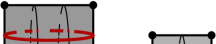
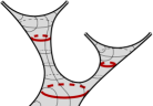
Figure 2. Square-tiled surface in $\mathcal{Q}_{0,7}$, and associated multicurve and stable graph

Suppose that the resulting closed square-tiled surface has genus $g$ and $n$ conical singularities with angle $\pi$, i.e. $n$ vertices adjacent to only two squares. For example, the square-tiled surfaces in Figure 2 has genus $g=0$ and $n=7$ conical singularities with angle $\pi$. Consider the complex coordinate $z$ in each square and a quadratic differential $(dz)^{2}$. It is easy to check that the resulting square-tiled surface inherits the complex structure and globally defined meromorphic quadratic differential $q$ having simple poles at $n$ conical singularities with angle $\pi$ and no other poles. Thus, any square-tiled surface of genus $g$ having $n$ conical singularities with angle $\pi$ canonically defines a point $(C,q)\in\mathcal{Q}_{g,n}$. Fixing the size of the square once and forever and considering all resulting square-tiled surfaces in $\mathcal{Q}_{g,n}$ we get a discrete subset $\mathcal{ST}{}_{g,n}$ in $\mathcal{Q}_{g,n}$.

Define $\mathcal{ST}{}_{g,n}(N)\subset\mathcal{ST}{}_{g,n}$ to be the subset of square-tiled surfaces in $\mathcal{Q}_{g,n}$ tiled with at most $N$ identical squares. Square-tiled surfaces form a lattice in period coordinates of $\mathcal{Q}_{g,n}$, which justifies the following alternative definition of the Masur–Veech volume:

(2.2) $$\operatorname{Vol}\mathcal{Q}_{g,n}=2(6g-6+2n)\cdot\lim_{N\to+\infty}\frac{\operatorname{card}(\mathcal{ST}{}_{g,n}(2N))}{N^{d}}\,,$$

where $d=6g-6+2n=\dim_{{\mathbb{C}}}\mathcal{Q}_{g,n}$. In this formula we assume that all conical singularities of square-tiled surfaces are labeled (i.e., counting square-tiled surfaces we label not only $n$ simple poles but also all zeroes).

Multicurve associated to a cylinder decomposition. Any square-tiled surface admits a decomposition into maximal horizontal cylinders filled with isometric closed regular flat geodesics. Every such maximal horizontal cylinder has at least one conical singularity on each of the two boundary components. The square-tiled surface in Figure 2 has four maximal horizontal cylinders which are represented in the picture by different shades. For every maximal horizontal cylinder choose the corresponding waist curve $\gamma_{i}$.

By construction each resulting simple closed curve $\gamma_{i}$ is non-periferal (i.e. it does not bound a topological disk without punctures or with a single puncture) and different $\gamma_{i},\gamma_{j}$ are not freely homotopic on the underlying $n$-punctured topological surface. In other words, pinching simultaneously all waist curves $\gamma_{i}$ we get a legal stable curve in the Deligne–Mumford compactification $\overline{\mathcal{M}}_{g,n}$.

We encode the number of circular horizontal bands of squares contained in the corresponding maximal horizontal cylinder by the integer weight $H_{i}$ associated to the curve $\gamma_{i}$. The above observation implies that the resulting formal linear combination $\gamma=\sum H_{i}\gamma_{i}$ is a simple closed integral multicurve in the space $\mathcal{ML}_{g,n}({\mathbb{Z}})$ of measured laminations. For example, the simple closed multicurve associated to the square-tiled surface as in Figure 2 has the form $2\gamma_{1}+\gamma_{2}+\gamma_{3}+2\gamma_{4}$.

Given a simple closed integral multicurve $\gamma$ in $\mathcal{ML}_{g,n}({\mathbb{Z}})$ consider the subset $\mathcal{ST}{}_{g,n}(\gamma)\subset\mathcal{ST}{}_{g,n}$ of those square-tiled surfaces, for which the associated horizontal multicurve is in the same $\operatorname{Mod}_{g,n}$-orbit as $\gamma$ (i.e. it is homeomorphic to $\gamma$ by a homeomorphism sending $n$ marked points to $n$ marked points and preserving their labeling). Denote by $\operatorname{Vol}(\gamma)$ the contribution to $\operatorname{Vol}\mathcal{Q}_{g,n}$ of square-tiled surfaces from the subset $\mathcal{ST}{}_{g,n}(\gamma)\subset\mathcal{ST}{}_{g,n}$:

$$\operatorname{Vol}(\gamma)=2(6g-6+2n)\cdot\lim_{N\to+\infty}\frac{\operatorname{card}(\mathcal{ST}{}_{g,n}(2N)\cap\mathcal{ST}{}_{g,n}(\gamma))}{N^{d}}\,.$$

The results in [DGZZ20a] imply that for any $\gamma$ in $\mathcal{ML}_{g,n}({\mathbb{Z}})$ the above limit exists, is strictly positive, and that

(2.3) $$\operatorname{Vol}\mathcal{Q}_{g,n}=\sum_{[\gamma]\in\mathcal{O}}\operatorname{Vol}(\gamma)\,,$$

where the sum is taken over representatives $[\gamma]$ of all orbits $\mathcal{O}$ of the mapping class group $\operatorname{Mod}_{g,n}$ in $\mathcal{ML}_{g,n}({\mathbb{Z}})$.

Definition 2.1.

Formula (2.3) allows to interpret the ratio $\operatorname{Vol}(\gamma)/\operatorname{Vol}\mathcal{Q}_{g,n}$ as the asymptotic probability to get a square-tiled surface in $\mathcal{ST}{}_{g,n}(\gamma)$ taking a random square-tiled surface in $\mathcal{ST}{}_{g,n}(N)$ as $N\to+\infty$. We will also call the same quantity by the frequency of square-tiled surfaces of type $\mathcal{ST}{}_{g,n}(\gamma)$ among all square-tiled surfaces.

Stable graph associated to a multicurve. Following M. Kontsevich [Kon92] we assign to any multicurve $\gamma$ a stable graph $\Gamma(\gamma)=\Gamma(\gamma_{\mathit{reduced}})$. The stable graph $\Gamma(\gamma)$ is a decorated graph dual to $\gamma_{reduced}$. It consists of vertices, edges, and “half-edges” also called “legs”. Vertices of $\Gamma(\gamma)$ represent the connected components of the complement $S_{g,n}\setminus\gamma_{\mathit{reduced}}$. Each vertex is decorated with the integer number recording the genus of the corresponding connected component of $S_{g,n}\setminus\gamma_{reduced}$. By convention, when this number is not explicitly indicated, it equals to zero. Edges of $\Gamma(\gamma)$ are in the natural bijective correspondence with curves $\gamma_{i}$; an edge joins a vertex to itself when on both sides of the corresponding simple closed curve $\gamma_{i}$ we have the same connected component of $S_{g,n}\setminus\gamma_{reduced}$. Finally, the $n$ punctures are encoded by $n$ legs. The right picture in Figure 2 provides an example of the stable graph associated to the multicurve $\gamma$.

Pinching a complex curve of genus $g$ with $n$ marked points by all components of a reduced multicurve $\gamma_{reduced}$ we get a stable complex curve representing a point in the Deligne–Mumford compactification $\overline{\mathcal{M}}_{g,n}$. In this way stable graphs encode the boundary cycles of $\overline{\mathcal{M}}_{g,n}$. In particular, the set $\mathcal{G}_{g,n}$ of all stable graphs is finite. It is in the natural bijective correspondence with boundary cycles of $\overline{\mathcal{M}}_{g,n}$ or, equivalently, with $\operatorname{Mod}_{g,n}$-orbits of reduced multicurves in $\mathcal{ML}_{g,n}({\mathbb{Z}})$.

2.3. Formula for the Masur–Veech volumes

In this section we introduce polynomials $N_{g,n}(b_{1},\ldots,b_{n})$ that appear in different contexts, in particular, in the formula for the Masur–Veech volume.

Let $g$ be a non-negative integer and $n$ a positive integer. Let the pair $(g,n)$ be different from $(0,1)$ and $(0,2)$. Let $d_{1},\dots,d_{n}$ be an ordered partition of $3g-3+n$ into a sum of non-negative integers, $|d|=d_{1}+\dots+d_{n}=3g-3+n$, let $\boldsymbol{d}$ be a multiindex $(d_{1},\dots,d_{n})$ and let $b^{2\boldsymbol{d}}$ denote $b_{1}^{2d_{1}}\cdot\cdots\cdot b_{n}^{2d_{n}}$.

Define the following homogeneous polynomial $N_{g,n}(b_{1},\dots,b_{n})$ of degree $6g-6+2n$ in variables $b_{1},\dots,b_{n}$ in the following way.

(2.4) $$N_{g,n}(b_{1},\dots,b_{n})=\sum_{|d|=3g-3+n}c_{\boldsymbol{d}}b^{2\boldsymbol{d}}\,,$$

where

(2.5) $$c_{\boldsymbol{d}}=\frac{1}{2^{5g-6+2n}\,\boldsymbol{d}!}\,\langle\tau_{d_{1}}\dots\tau_{d_{n}}\rangle_{g,n}$$

(2.6) $$\langle\tau_{d_{1}}\dots\tau_{d_{n}}\rangle_{g,n}=\int_{\overline{\mathcal{M}}_{g,n}}\psi_{1}^{d_{1}}\dots\psi_{n}^{d_{n}}\,,$$

and $\boldsymbol{d}!=d_{1}!\cdots d_{n}!$. Note that $N_{g,n}(b_{1},\dots,b_{n})$ contains only even powers of $b_{i}$, where $i=1,\dots,n$.

Following [AEZ16] we consider the following linear operators $\mathcal{Y}(\boldsymbol{H})$ and $\mathcal{Z}$ on the spaces of polynomials in variables $b_{1},b_{2},\dots$, where $H_{1},H_{2},\dots$ are positive integers. The operator $\mathcal{Y}(\boldsymbol{H})$ is defined on monomials as

(2.7) $$\mathcal{Y}(\boldsymbol{H})\ :\quad\prod_{i=1}^{k}b_{i}^{m_{i}}\longmapsto\prod_{i=1}^{k}\frac{m_{i}!}{H_{i}^{m_{i}+1}}\,,$$

and extended to arbitrary polynomials by linearity. The operator $\mathcal{Z}$ is defined on monomials as

(2.8) $$\mathcal{Z}\ :\quad\prod_{i=1}^{k}b_{i}^{m_{i}}\longmapsto\prod_{i=1}^{k}\big{(}m_{i}!\cdot\zeta(m_{i}+1)\big{)}\,,$$

and extended to arbitrary polynomials by linearity.

Given a stable graph $\Gamma$ denote by $V(\Gamma)$ the set of its vertices and by $E(\Gamma)$ the set of its edges. To each stable graph $\Gamma\in\mathcal{G}_{g,n}$ we associate the following homogeneous polynomial $P_{\Gamma}$ of degree $6g-6+2n$. To every edge $e\in E(\Gamma)$ we assign a formal variable $b_{e}$. Given a vertex $v\in V(\Gamma)$ denote by $g_{v}$ the integer number decorating $v$ and denote by $n_{v}$ the valency of $v$, where the legs adjacent to $v$ are counted towards the valency of $v$. Take a small neighborhood of $v$ in $\Gamma$. We associate to each half-edge (“germ” of edge) $e$ adjacent to $v$ the monomial $b_{e}$; we associate $0$ to each leg. We denote by $\boldsymbol{b}_{v}$ the resulting collection of size $n_{v}$. If some edge $e$ is a loop joining $v$ to itself, $b_{e}$ would be present in $\boldsymbol{b}_{v}$ twice; if an edge $e$ joins $v$ to a distinct vertex, $b_{e}$ would be present in $\boldsymbol{b}_{v}$ once; all the other entries of $\boldsymbol{b}_{v}$ correspond to legs; they are represented by zeroes. To each vertex $v\in E(\Gamma)$ we associate the polynomial $N_{g_{v},n_{v}}(\boldsymbol{b}_{v})$, where $N_{g,v}$ is defined in (2.4). We associate to the stable graph $\Gamma$ the polynomial obtained as the product $\prod b_{e}$ over all edges $e\in E(\Gamma)$ multiplied by the product $\prod N_{g_{v},n_{v}}(\boldsymbol{b}_{v})$ over all $v\in V(\Gamma)$. We define $P_{\Gamma}$ as follows:

(2.9) $$P_{\Gamma}(\boldsymbol{b})=\frac{2^{6g-5+2n}\cdot(4g-4+n)!}{(6g-7+2n)!}\cdot\\ \frac{1}{2^{|V(\Gamma)|-1}}\cdot\frac{1}{|\operatorname{Aut}(\Gamma)|}\cdot\prod_{e\in E(\Gamma)}b_{e}\cdot\prod_{v\in V(\Gamma)}N_{g_{v},n_{v}}(\boldsymbol{b}_{v})\,.$$

Theorem ([DGZZ19]).

The Masur–Veech volume $\operatorname{Vol}\mathcal{Q}_{g,n}$ of the stratum of quadratic differentials with $4g-4+n$ simple zeros and $n$ simple poles has the following value:

(2.10) $$\operatorname{Vol}\mathcal{Q}_{g,n}=\sum_{\Gamma\in\mathcal{G}_{g,n}}\operatorname{Vol}(\Gamma)\,,$$

where the contribution of an individual stable graph $\Gamma$ has the form

(2.11) $$\operatorname{Vol}(\Gamma)=\mathcal{Z}(P_{\Gamma})\,.$$

Remark 2.2.

The contribution (2.11) of any individual stable graph has the following natural interpretation. We have seen that stable graphs $\Gamma$ in $\mathcal{G}_{g,n}$ are in natural bijective correspondence with $\operatorname{Mod}_{g,n}$-orbits of reduced multicurves $\gamma_{\mathit{reduced}}=\gamma_{1}+\gamma_{2}+\dots$, where simple closed curves $\gamma_{i}$ and $\gamma_{j}$ are not isotopic for any $i\neq j$. Let $\Gamma\in\mathcal{G}_{g,n}$, let $k=|V(\Gamma)|$, let $\gamma_{\mathit{reduced}}=\gamma_{1}+\dots+\gamma_{k}$ be the reduced multicurve associated to $\Gamma$. Let $\gamma_{\boldsymbol{H}}=\gamma(\Gamma,\boldsymbol{H})=H_{1}\gamma_{1}+\dots H_{k}\gamma_{k}$, where $\boldsymbol{H}=(H_{1},\dots,H_{k})\in{\mathbb{N}}^{k}$. We have

(2.12) $$\operatorname{Vol}(\Gamma)=\sum_{H\in{\mathbb{N}}^{k}}\operatorname{Vol}\big{(}\Gamma,\boldsymbol{H}\big{)}$$

where the contribution $\operatorname{Vol}\big{(}\Gamma,\boldsymbol{H})$ of square-tiled surfaces with the horizontal cylinder decomposition of type $(\Gamma,\boldsymbol{H})$ to $\operatorname{Vol}\mathcal{Q}_{g,n}$ is given by the formula:

(2.13) $$\operatorname{Vol}\big{(}\Gamma,\boldsymbol{H}\big{)}=\mathcal{Y}(\boldsymbol{H})(P_{\Gamma})\,.$$

In other words, we can rearrange the sum in (2.3) as

(2.14) $$\operatorname{Vol}\mathcal{Q}_{g,n}=\sum_{[\gamma]\in\mathcal{O}}\operatorname{Vol}(\gamma)=\sum_{\Gamma\in\mathcal{G}_{g,n}}\sum_{\{[\gamma]\,|\Gamma(\gamma)=\Gamma\}}\operatorname{Vol}(\gamma)\,,$$

where

$$\sum_{\{[\gamma]\,|\,\Gamma(\gamma)=\Gamma\}}\operatorname{Vol}(\gamma)=\operatorname{Vol}(\Gamma)\,.$$

In this way we can extend Definition 2.1 and speak of asymptotic probability of getting a square-tiled surface in $\mathcal{ST}{}_{g,n}(\Gamma)=\cup_{\{[\gamma]\,|\,\Gamma(\gamma)=\Gamma\}}\mathcal{ST}{}_{g,n}(\gamma)$ taking a random square-tiled surface in $\mathcal{ST}{}_{g,n}(N)$ as $N\to+\infty$. In the same way we define frequency of square-tiled surfaces having exactly $k$ maximal horizontal cylinders among all square-tiled surfaces of genus $g$.

In particular, we define the quantity ${\mathbb{P}}\big{(}K_{g}(S)=k\big{)}$ from Equation (1.6) as

(2.15) $${\mathbb{P}}\big{(}K_{g}(S)=k\big{)}=\frac{1}{\operatorname{Vol}\mathcal{Q}_{g}}\cdot\sum_{\begin{subarray}{c}\Gamma\in\mathcal{G}_{g}\\ |V(\Gamma)|=k\end{subarray}}\operatorname{Vol}(\Gamma)\,.$$

We complete this section with the theorem which is one of the two keystone results on which rely all further asymptotic results of the current paper. Morally, it serves to establish explicit normalization allowing to pass from a finite measure with unspecified total mass to a specific probability measure. This statement was conjectured in [DGZZ19] and proved in [Ag20b, Theorem 1.7].

Theorem 2.3 (A. Aggarwal [Ag20b]).

The Masur–Veech volume of the moduli space of holomorphic quadratic differentials has the following large genus asymptotics:

(2.16) $$\operatorname{Vol}\mathcal{Q}_{g}=\frac{4}{\pi}\cdot\left(\frac{8}{3}\right)^{4g-4}\cdot\big{(}1+o(1)\big{)}\quad\text{as }g\to+\infty\,.$$

Remark 2.4.

The exact values of $\operatorname{Vol}\mathcal{Q}_{g}$ for $g\leq 250$ (and more) can be obtained by combining results of D. Chen, M. Möller, A. Sauvaget [CMöS19] with the results of M.Kazarian [Kaz20] or with the results of D. Yang, D. Zagier and Y. Zhang [YZZ20]. Supported by serious data analysis, the authots of [YZZ20] conjecture that the error term in (2.16) admits an asymptotic expansion in $g^{-1}$ with the leading term $-\frac{\pi^{2}}{144}\cdot\frac{1}{g}$ and with explicit coefficients for the terms $g^{-2}$ and $g^{-3}$. In Theorem 5.1, using a refinement of the estimates from [Ag20b] we prove that the error term $o(1)$ in 2.16 can be improved to a finer estimate $O(g^{-1/4})$.

Conjectural generalization of formula (2.16) to all strata of meromorphic quadratic differentials and numerical evidence beyond this conjecture are presented in [ADGZZ19]. Actually, [Ag20b, Theorem 1.7] proves the volume asymptotics in the more general setting for $\operatorname{Vol}\mathcal{Q}_{g,n}$ under assumption that the number $n$ of simple poles satisfies the relation $20n<\log g$.

2.4. Frequencies of multicurves (after M. Mirzakhani)

Recall that two integral multicurves on the same smooth surface of genus $g$ with $n$ punctures have the same topological type if they belong to the same orbit of the mapping class group $\operatorname{Mod}_{g,n}$.

We change now flat setting to hyperbolic setting. Following M. Mirzakhani, given an integral multicurve $\gamma$ in $\mathcal{ML}_{g,n}({\mathbb{Z}})$ and a hyperbolic surface $X\in\mathcal{T}_{g,n}$ consider the function $s_{X}(L,\gamma)$ counting the number of simple closed geodesic multicurves on $X$ of length at most $L$ of the same topological type as $\gamma$. M. Mirzakhani proves in [Mi08a] the following Theorem.

Theorem (M. Mirzakhani).

For any rational multi-curve $\gamma$ and any hyperbolic surface $X\in\mathcal{T}_{g,n}$,

(2.17) $$s_{X}(L,\gamma)\sim B(X)\cdot\frac{c(\gamma)}{b_{g,n}}\cdot L^{6g-6+2n}\,,$$

as $L\to+\infty$.

The factor $B(X)$ in the above formula has the following geometric meaning. Consider the unit ball $B_{X}=\{\gamma\in\mathcal{ML}_{g,n}\,|\,\ell_{X}(\gamma)\leq 1\}$ defined by means of the length function $\ell_{X}$. The factor $B(X)$ is the Thurston’s measure of $B_{X}$:

$$B(X)=\mu_{\mathrm{Th}}(B_{X})\,.$$

The factor $b_{g,n}$ is defined as the average of $B(X)$ over $\mathcal{M}_{g,n}$ viewed as the moduli space of hyperbolic metrics, where the average is taken with respect to the Weil–Petersson volume form on $\mathcal{M}_{g,n}$:

(2.18) $$b_{g,n}=\int_{\mathcal{M}_{g,n}}B(X)\,dX\,.$$

Mirzakhani showed that

(2.19) $$b_{g,n}=\sum_{[\gamma]\in\mathcal{O}(g,n)}c(\gamma)\,,$$

where the sum of $c(\gamma)$ taken with respect to representatives $[\gamma]$ of all orbits $\mathcal{O}(g,n)$ of the mapping class group $\operatorname{Mod}_{g,n}$ in $\mathcal{ML}_{g,n}({\mathbb{Z}})$. This allows to interpret the ratio $\tfrac{c(\gamma)}{b_{g,n}}$ as the probability to get a multicurve of type $\gamma$ taking a “large random” multicurve (in the same sense as the probability that coordinates of a “random” point in ${\mathbb{Z}}^{2}$ are coprime equals $\tfrac{6}{\pi^{2}}$).

In particular, we define the quantity ${\mathbb{P}}\big{(}K_{g}(\gamma)=k\big{)}$ from Equation (1.6) as

(2.20) $${\mathbb{P}}\big{(}K_{g}(\gamma)=k\big{)}=\frac{1}{b_{g}}\cdot\sum_{[\gamma]\in\mathcal{O}_{k}(g)}c(\gamma)\,,$$

where, $b_{g}=b_{g,0}$ and $\mathcal{O}_{k}(g)\subset\mathcal{O}(g)=\mathcal{O}(g,0)$ is the subcollection of orbits of those multicurves $\gamma$, for which $\gamma_{\mathit{reduced}}$ has exactly $k$ connected components.

M. Mirzakhani found an explicit expression for the coefficient $c(\gamma)$ and for the global normalization constant $b_{g,n}$ in terms of the intersection numbers of $\psi$-classes.

2.5. Frequencies of square-tiled surfaces of fixed combinatorial type

The following Theorem bridges flat and hyperbolic count.

Theorem ([DGZZ19]).

For any integral multicurve $\gamma\in\mathcal{ML}_{g,n}({\mathbb{Z}})$, the volume contribution $\operatorname{Vol}(\gamma)$ to the Masur–Veech volume $\operatorname{Vol}\mathcal{Q}_{g,n}$ coincides with the Mirzakhani’s asymptotic frequency $c(\gamma)$ of simple closed geodesic multicurves of topological type $\gamma$ up to the explicit factor $const_{g,n}$ depending only on $g$ and $n$:

(2.21) $$\operatorname{Vol}(\gamma)=const_{g,n}\cdot c(\gamma)\,,$$

where

(2.22) $$const_{g,n}=2\cdot(6g-6+2n)\cdot(4g-4+n)!\cdot 2^{4g-3+n}\cdot$$

Proof of Theorem 1.7.

Definitions (2.15) and (2.20) and Formulae (2.14) and (2.19) combined with relation (2.21) imply that ${\mathbb{P}}\big{(}K_{g}(\gamma)=k\big{)}={\mathbb{P}}\big{(}K_{g}(S)=k\big{)}$. ∎

Corollary ([DGZZ19]).

For any admissible pair of non-negative integers $(g,n)$ different from $(1,1)$ and $(2,0)$, the Masur–Veech volume $\operatorname{Vol}\mathcal{Q}_{g,n}$ and the average Thurston measure of a unit ball $b_{g,n}$ are related as follows:

(2.23) $$\operatorname{Vol}\mathcal{Q}_{g,n}=2\cdot(6g-6+2n)\cdot(4g-4+n)!\cdot 2^{4g-3+n}\cdot b_{g,n}\,.$$

Remark 2.5.

In Theorem 1.4 in [Mi08b] M. Mirzakhani established the relation

$$\operatorname{Vol}\mathcal{Q}_{g}=const_{g}\cdot b_{g}\,,$$

where $b_{g}$ is computed in Theorem 5.3 in [Mi08a]. However, Mirzakhani does not give any formula for the value of the normalization constant $const_{g}$ presented in (2.23). This constant was recently computed by F. Arana–Herrera [AH20a] and by L. Monin and I. Telpukhovskiy [MoT19] simultaneously and independently of us by different methods. The same value of $const_{g,n}$ is obtained by V. Erlandsson and J. Souto in [ErSo20] through an approach different from all the ones mentioned above.

2.6. Uniform large genus asymptotics of correlators (after A. Aggarwal)

We denote by $\Pi(m,n)$ the set of nonnegative compositions of an integer $m$ as sum of $n$ non-negative integers. For any nonnegative composition $\boldsymbol{d}\in\Pi(3g-3+n,n)$ define $\varepsilon(\boldsymbol{d})$ through the following equation:

(2.24) $$\langle\tau_{d_{1}}\dots\tau_{d_{n}}\rangle_{g,n}=\frac{(6g-5+2n)!!}{(2d_{1}+1)!!\cdots(2d_{n}+1)!!}\cdot\frac{1}{g!\cdot 24^{g}}\cdot\big{(}1+\varepsilon(\boldsymbol{d})\big{)}\,.$$

By construction, the intersection numbers are nonnegative rational numbers, so $\varepsilon\big{(}\boldsymbol{d}\big{)}\geq-1$ for any $\boldsymbol{d}\in\Pi(3g-3+n,n)$. We conjectured in [DGZZ19] that $\varepsilon(\boldsymbol{d})$ tends to zero uniformly for all nonnegative compositions $\boldsymbol{d}\in\Pi(3g-3+n,n)$ as soon as $n\leq 2\log g$ and $g\to+\infty$. This conjecture was proved in much stronger form in the recent paper of A. Aggarwal [Ag20b].

The following Theorem corresponds to [Ag20b, Proposition 1.2].

Theorem 2.6 (A. Aggarwal).

Let $n\in\mathbb{Z}_{\geq 1}$ and $\boldsymbol{d}\in\mathbb{Z}_{\geq 0}^{n}$ satisfy $|\boldsymbol{d}|=3g+n-3$, for some $g\in\mathbb{Z}_{\geq 0}$. Then,

(2.25) $$1+\varepsilon(\boldsymbol{d})\leq\left(\frac{3}{2}\right)^{n-1}\,.$$

The next Theorem corresponds to [Ag20b, Proposition 4.1].

Theorem 2.7 (A. Aggarwal).

Let $g>2^{15}$ and $n\geq 1$ be integers such that $g>30n$, and let $\boldsymbol{d}\in\Pi(3g-3+n,n)$. Then we have

(2.26) $$\varepsilon(\boldsymbol{d})\geq-20\cdot\frac{(n+4\log g)}{g}\,.$$

Finally, the following Theorem corresponds to [Ag20b, Proposition 4.2].

Theorem 2.8 (A. Aggarwal).

Let $g>2^{30}$ and $n\geq 1$ be integers such that $g>800n^{2}$, and let $\boldsymbol{d}\in\Pi(3g-3+n,n)$. Then we have

(2.27) $$1+\varepsilon(\boldsymbol{d})\leq\exp\left(625\cdot\frac{(n+2\log g)^{2}}{g}\right)\,.$$

Remark 2.9.

We proved in [DGZZ19] explicit sharp upper and lower bounds for $2$-correlators.

3. Random non-separating multicurves and non-uniform random permutations

Consider the stable graph $\Gamma_{k}(g)$ having a single vertex, decorated with genus $g-k$, and having $k$ loops, see the left picture in Figure 3. This stable graph corresponds to multicurves on a closed surface of genus $g$, for which the components $\gamma_{1},\dots,\gamma_{k}$ of the underlying reduced multicurve $\gamma_{\mathit{reduced}}=\gamma_{1}+\dots+\gamma_{k}$ represent $k$ linearly independent homology cycles. The square-tiled surfaces associated to this stable graph have single horizontal singular layer and $k$ maximal horizontal cylinders.

Figure 3. The stable graph $\Gamma_{k}(g)$ (on the left) corresponds to the reduced multicurve $\gamma_{\mathit{reduced}}=\gamma_{1}+\dots+\gamma_{k}$ represented by $k$ linearly independent homology cycles on a surface of genus $g$ (on the right).

Recall from Section 2.3 that by $\operatorname{Vol}(\Gamma_{k}(g))$ we denote the volume contribution from all square-tiled surfaces corresponding to the stable graph $\Gamma_{k}(g)$. By $\operatorname{Vol}\big{(}\Gamma_{k}(g),(m_{1},\ldots,m_{k}))$ we denote the volume contribution from those square-tiled surfaces corresponding to the stable graph $\Gamma_{k}(g)$ for which one maximal horizontal cylinder is filled with $m_{1}$ bands of squares, another cylinder is filled with $m_{2}$ bands of squares, and so on up to the $k$th maximal horizontal cylinder, which is filled with $m_{k}$ bands of squares. The corresponding multicurve has the form $m_{1}\gamma_{1}+\dots+m_{k}\gamma_{k}$, where $\gamma_{1},\dots,\gamma_{k}$ are as described above. By (2.12) we have

$$\operatorname{Vol}(\Gamma_{k}(g))=\sum_{\begin{subarray}{c}m_{1},\ldots,m_{k}\\ 1\leq m_{i}\leq m\ \text{for }i=1,\dots,k\end{subarray}}\operatorname{Vol}\big{(}\Gamma_{k}(g),(m_{1},\ldots,m_{k})).$$

In this section we prove the following result, which relies on the uniform asymptotics of Witten correlators proved by A. Aggarwal (see Theorems 2.6–2.8 in the current paper or Propositions 1.2, 4.1, 4.2 respectively in the original paper [Ag20b] of A. Aggarwal).

Theorem 3.1.

Let $m\in{\mathbb{N}}\cup\{+\infty\}$. For any complex number $t$, in the disk $|t|<2$ we have as $g\to+\infty$

(3.1) $$\sum_{k=1}^{g}\quad\sum_{\begin{subarray}{c}m_{1},\ldots,m_{k}\\ 1\leq m_{i}\leq m\ \text{for }i=1,\dots,k\end{subarray}}\operatorname{Vol}(\Gamma_{k}(g),(m_{1},\ldots,m_{k}))\cdot t^{k}=\\ =\frac{2\sqrt{2}\left(\frac{2m}{m+1}\right)^{t/2}}{\sqrt{\pi}\cdot\Gamma(\frac{t}{2})}\cdot(3g-3)^{\frac{t-1}{2}}\cdot\left(\frac{8}{3}\right)^{4g-4}\left(1+O\left(\frac{(\log g)^{2}}{g}\right)\right)\,,$$

where for every compact subset $U$ of the complex disk $|t|<2$ the error term is uniform over $m\in{\mathbb{N}}\cup\{+\infty\}$ and $t\in U$. In particular, for $m=+\infty$ and $t=1$ we obtain

(3.2) $$\sum_{k=1}^{g}\operatorname{Vol}(\Gamma_{k}(g))=\frac{4}{\pi}\left(\frac{8}{3}\right)^{4g-4}\left(1+O\left(\frac{(\log g)^{2}}{g}\right)\right)\,.$$

We prove Theorem 3.1 in Section 3.7. We note that asymptotics (3.2) was first obtained by A. Aggarwal in [Ag20b, Proposition 8.3]. Our refinement consists in the bound $O\left(\frac{(\log g)^{2}}{g}\right)$ for the error term. Conjecturally, the bound can be further improved to $O\left(\frac{1}{g}\right)$; see Remark 2.4.

3.1. Volume contribution of stable graphs with a single vertex

In this section, we show how to express an approximate value of the contribution $\operatorname{Vol}(\Gamma_{k}(g))$ of square-tiled surfaces corresponding to the stable graph $\Gamma_{k}(g)$ to the Masur–Veech volume $\operatorname{Vol}\mathcal{Q}_{g}$ in terms of the following normalized weighted multi-variate harmonic sum.

Definition 3.2.

Let $m\in{\mathbb{N}}\cup\{+\infty\}$ and let $\alpha$ be a positive real number. For integers $k,n$ such that $1\leq k\leq n$, define

(3.3) $$\widetilde{H}_{n,m,\alpha}(k)=\frac{\alpha^{k}}{k!}\sum_{j_{1}+\dots+j_{k}=n}\frac{\zeta_{m}(2j_{1})\cdot\zeta_{m}(2j_{2})\cdots\zeta_{m}(2j_{k})}{j_{1}\cdot j_{2}\cdots j_{k}}\,,$$

where the sum is taken over all $k$-tuples $(j_{1},j_{2},\ldots,j_{k})\in{\mathbb{N}}^{k}$ of positive integers summing up to $n$ and

$$\zeta_{m}(s)=1+\frac{1}{2^{s}}+\frac{1}{3^{s}}+\ldots+\frac{1}{m^{s}}$$

is the partial zeta function.

Remark 3.3.

The particular cases of the above numbers, namely,

$$H_{k}(n)=\sum_{j_{1}+\dots+j_{k}=n} \frac{1}{j_{1}\cdot j_{2}\cdots j_{k}}=k!\cdot\widetilde{H}_{n,1,1}(k)$$

$$\ Z_{k}(n)=\sum_{j_{1}+\dots+j_{k}=m} \frac{\zeta(2j_{1})\cdots\zeta(2j_{k})}{j_{1}\cdot j_{2}\cdots j_{k}}=k!\cdot\widetilde{H}_{n,\infty,1}(k)$$

appeared in the preprint [DGZZ19]; the asymptotic expansions for these quantities were obtained by A. Aggarwal in Sections 6 and 7 of [Ag20b]. The framework which we develop here allows to treat all normalized weighted multi-variate harmonic sums $\widetilde{H}_{n,m,\alpha}(k)$ in a unified way.

Theorem 3.4.

There exists a constant $C_{1}$ such that for sufficiently large $g\in{\mathbb{N}}$ the following property holds. For any couple $m,k$, such that $m\in{\mathbb{N}}\cup\{+\infty\}$, $k\in{\mathbb{N}}$, $800k^{2}\leq g$, we have

(3.4) $$\sum_{\begin{subarray}{c}m_{1},\ldots,m_{k}\\ 1\leq m_{i}\leq m\ \text{for }i=1,\dots,k\end{subarray}}\operatorname{Vol}\big{(}\Gamma_{k}(g),(m_{1},\ldots,m_{k})\big{)}=\\ =\frac{2\sqrt{2}}{\sqrt{\pi}}\cdot\sqrt{3g-3}\cdot\left(\frac{8}{3}\right)^{4g-4}\cdot\widetilde{H}_{3g-3,m,\frac{1}{2}}(k)\cdot\big{(}1+\varepsilon_{1}(g,k)\big{)}\,,$$

where $|\varepsilon_{1}(g,k)|\leq C_{1}\cdot\cfrac{(k+2\log g)^{2}}{g}$.

There exists a constant $C_{2}$ such that for all triples $(g,k,m)$, where $g\in{\mathbb{N}}$, $g\geq 2$; $k\in{\mathbb{N}}$, $k\leq g$; $m\in{\mathbb{N}}\cup\{+\infty\}$, we have

(3.5) $$\sum_{\begin{subarray}{c}m_{1},\ldots,m_{k}\\ 1\leq m_{i}\leq m\ \text{for }i=1,\dots,k\end{subarray}}\operatorname{Vol}\big{(}\Gamma_{k}(g),(m_{1},\ldots,m_{k})\big{)}\leq\\ \leq C_{2}\cdot\sqrt{g}\cdot\left(\frac{8}{3}\right)^{4g-4}\cdot\widetilde{H}_{3g-3,m,\frac{1}{2}}(k)\cdot\left(\frac{9}{4}\right)^{k}\,,$$

where $\widetilde{H}_{3g-3,m,\frac{1}{2}}(k)$ is the normalized weighted multi-variate harmonic sum defined in (3.3).

In order to prove Theorem 3.4 we first state and prove Lemma 3.5 below.

Let $\textbf{D}=(D_{1},\dots,D_{k})\in\Pi(3g-3+2k,k)$. Define $c_{g,k}(\boldsymbol{D})$ as

(3.6) $$c_{g,k}(\boldsymbol{D}):=\frac{g!\cdot(3g-3+2k)!}{(6g+4k-5)!}\cdot\frac{3^{g}}{2^{3g-6+5k}}\cdot\\ \cdot\sum_{d_{1,1}+d_{1,2}=D_{1}}\dots\sum_{d_{k,1}+d_{k,2}=D_{k}}\int_{\overline{\mathcal{M}}_{g,2k}}\psi_{1}^{d_{1,1}}\psi_{2}^{d_{1,2}}\dots\psi_{2k-1}^{d_{k,1}}\psi_{2k}^{d_{k,2}}\cdot\prod_{j=1}^{k}\cfrac{(2D_{j}+2)!}{d_{j,1}!\cdot d_{j,2}!}\,.$$

The following result is a corollary of the uniform asymptotics of Witten correlators proved by A. Aggarwal (see Theorems 2.6–2.8 in the current paper or Propositions 1.2, 4.1, 4.2 respectively in the original paper [Ag20b] of A. Aggarwal).

Lemma 3.5.

There exists a constant $C_{3}$ such that for sufficiently large $g\in{\mathbb{N}}$ and for $k\in{\mathbb{N}}$ satisfying $800k^{2}\leq g$ we have

(3.7) $$|c_{g,k}(\boldsymbol{D})-1|\leq C_{3}\cdot\frac{(k+2\log g)^{2}}{g}\,.$$

For any positive integers $g,k\in{\mathbb{N}}$ satisfying $1\leq k\leq g$ and $g\geq 2$, we have

(3.8) $$c_{g,k}(\boldsymbol{D})\leq\left(\frac{9}{4}\right)^{k}.$$

Proof.

Passing to double factorials and applying definition (2.24) of $\varepsilon(\boldsymbol{d})$ we get

$$c_{g,k}(\boldsymbol{D})=\frac{g!}{2^{3g-3+2k}\cdot(6g+4k-5)!!}\cdot\frac{3^{g}}{2^{3g-6+5k}}\cdot\\ \cdot\sum_{d_{1,1}+d_{1,2}=D_{1}}\dots\sum_{d_{k,1}+d_{k,2}=D_{k}}\langle\tau_{d_{1,1}}\tau_{d_{1,2}}\dots\tau_{d_{k,1}}\tau_{d_{k,2}}\rangle_{g,2k}\\ \prod_{j=1}^{k}\left(\frac{(2d_{j,1}+1)!}{d_{j,1}!}\cdot\frac{(2d_{j,2}+1)!}{d_{j,2}!}\cdot\binom{2D_{j}+2}{2d_{j,1}+1}\right)=\\ =\frac{1}{2^{6g-6+5k}}\sum_{d_{1,1}+d_{1,2}=D_{1}}\dots\sum_{d_{k,1}+d_{k,2}=D_{k}}\left(\big{(}1+\varepsilon(\boldsymbol{d})\big{)}\cdot\prod_{j=1}^{k}\binom{2D_{j}+2}{2d_{j,1}+1}\right)\,.$$

Applying the combinatorial identity

$$\sum_{m=0}^{n-1}\binom{2n}{2m+1}=2^{2n-1}$$

we get

$$\sum_{d_{1,1}+d_{1,2}=D_{1}}\dots\sum_{d_{k,1}+d_{k,2}=D_{k}}\prod_{j=1}^{k}\binom{2D_{j}+2}{2d_{j,1}+1}=\\ =\left(\prod_{j=1}^{k}\sum_{d_{j,1}=0}^{D_{j}}\binom{2D_{j}+2}{2d_{j,1}+1}\right)=\left(\prod_{j=1}^{k}2^{2D_{j}+1}\right)=2^{6g-6+5k}\,.$$

The claim that bound (3.7) is valid for sufficiently large $g$ now follows from combination of bounds (2.26) and (2.27) from Theorems 2.7 and 2.8 of A. Aggarwal (see Propositions 4.1, 4.2 respectively in the original paper [Ag20b]).

For $k\geq 2$ the universal bound (3.8) follows from the universal bound (2.25) from Theorem 2.6 of A. Aggarwal (see Proposition 1.2 in the original paper [Ag20b]), using the fact that for $k\geq 2$ we have $1+(3/2)^{2k-1}\leq(3/2)^{2k}$.

We prove in Proposition 4.1 in [DGZZ19] that $\varepsilon(\boldsymbol{d})\leq 0$ for any $\boldsymbol{d}\in\Pi(3g-1,2)$. This implies bound (3.8) for $k=1$, which completes the proof of the Lemma. ∎

Proof of Theorem 3.4.

Let us denote

(3.9) $$V_{m,k}(g)=\!\!\!\!\sum_{\begin{subarray}{c}m_{1},\ldots,m_{k}\\ 1\leq m_{i}\leq m\\ \text{for }i=1,\dots,k\end{subarray}}\!\!\!\operatorname{Vol}(\Gamma_{k}(g),(m_{1},\ldots,m_{k}))\quad\text{and}\quad V_{m}(g)=\sum_{k=1}^{g}V_{m,k}(g)\,.$$

The automorphism group $\operatorname{Aut}(\Gamma_{k}(g))$ consists of all possible permutations of loops composed with all possible flips of individual loops, so

$$|\operatorname{Aut}(\Gamma)|=2^{k}\cdot k!\,.$$

The graph $\Gamma_{k}(g)$ has a single vertex, so $|V(\Gamma_{k}(g)|=1$. Thus, applying (2.13) to $\Gamma_{k}(g)$ we get

(3.10) $$V_{m,k}(g)=\frac{2^{6g-5}\cdot(4g-4)!}{(6g-7)!}\cdot\\ 1\cdot\frac{1}{2^{k}\cdot k!}\cdot\sum_{\begin{subarray}{c}\boldsymbol{H}=(m_{1},\ldots,m_{k})\\ m_{1},\ldots,m_{k}\leq m\end{subarray}}\mathcal{Y}\big{(}\boldsymbol{H},b_{1}b_{2}\dots b_{k}\cdot N_{g-k,2k}(b_{1},b_{1},b_{2},b_{2},\dots,b_{k},b_{k})\big{)}=\\ =\frac{(4g-4)!}{(6g-7)!}\cdot\frac{2^{6g-5}}{2^{k}\cdot k!}\cdot\frac{1}{2^{5(g-k)-6+4k}}\cdot\\ \sum_{\boldsymbol{d}\in\Pi(3g-3-k,2k)}\frac{\langle\tau_{\mathbf{d}}\rangle_{g-k,2k}}{\mathbf{d}!}\,\cdot\,\prod_{i=1}^{k}\Big{(}(2d_{2i-1}+2d_{2i}+1)!\,\cdot\,\zeta_{m}(2d_{2i-1}+2d_{2i}+2)\Big{)}\,.$$

Rewrite the latter sum using notations $\textbf{D}=(D_{1},\dots,D_{k})\in\Pi(3g-3-k,k)$ and $c_{g-k,k}(\boldsymbol{D})$ defined by (3.6). Adjusting expression (3.6) given for genus $g$ to genus $g-k$ we get

$$\sum_{\boldsymbol{d}\in\Pi(3g-3-k,2k)}\frac{\langle\tau_{\mathbf{d}}\rangle_{g-k,2k}}{\mathbf{d}!}\,\cdot\,\prod_{i=1}^{k}\Big{(}(2d_{2i-1}+2d_{2i}+1)!\,\cdot\,\zeta_{m}(2d_{2i-1}+2d_{2i}+2)\Big{)}=\\ =\sum_{\boldsymbol{D}\in\Pi(3g-3-k,k)}c_{g-k,k}(\boldsymbol{D})\cdot\frac{(6(g-k)+4k-5)!}{(g-k)!\cdot(3(g-k)-3+2k)!}\cdot\frac{2^{3(g-k)-6+5k}}{3^{(g-k)}}\cdot\\ \cdot\prod_{j=1}^{k}\frac{\zeta_{m}(2D_{j}+2)}{2D_{j}+2}\,,$$

which allows to rewrite (3.10) as

(3.11) $$V_{m,k}(g)=\\ =\left(\frac{(4g-4)!}{(6g-7)!}\cdot 2^{g+1}\cdot\frac{1}{k!}\right)\cdot\left(\frac{(6g-2k-5)!}{(g-k)!\cdot(3g-3-k)!}\cdot\frac{2^{3g-6+2k}}{3^{g-k}}\right)\cdot\\ \sum_{\boldsymbol{D}\in\Pi(3g-3-k,2k)}\frac{c_{g-k,k}(\boldsymbol{D})}{2^{k}}\cdot\prod_{j=1}^{k}\frac{\zeta_{m}(2D_{j}+2)}{D_{j}+1}\,.$$

Let us define

$$c^{min}_{g-k,k}:=\min_{\boldsymbol{D}}c_{g-k,k}(\boldsymbol{D})\quad\text{and}\quad c^{max}_{g-k,k}:=\max_{\boldsymbol{D}}c_{g-k,k}(\boldsymbol{D})\,.$$

Rearranging factors with factorials, collecting powers of $2$ and $3$, and passing to notation $\widetilde{H}_{m,3g-3,\frac{1}{2}}(k)$ for the multivariate harmonic sum (3.3) we get the following bounds:

(3.12) $$c^{min}_{g-k,k}\leq V_{m,k}(g)\cdot\\ \left(\frac{(6g-2k-5)!}{(6g-7)!}\cdot\frac{(4g-4)!}{(g-k)!\cdot(3g-3-k)!}\cdot\frac{2^{4g-5+2k}}{3^{g-k}}\cdot\widetilde{H}_{3g-3,m,\frac{1}{2}}(k)\right)^{-1}\\ \leq c^{max}_{g-k,k}\,.$$

We start by proving the first assertion of the theorem represented by relation (3.4). We rewrite the product of factorials in (3.12) as

(3.13) $$\frac{(6g-2k-5)!\cdot(4g-4)!}{(6g-7)!\cdot(g-k)!\cdot(3g-3-k)!}=(6g-6)\cdot\binom{4g-4}{g-1}\cdot\frac{\frac{(3g-3)!}{(3g-3-k)!}\cdot\frac{(g-1)!}{(g-k)!}}{\frac{(6g-6)!}{(6g-2k-5)!}}\\ =(6g-6)\cdot\binom{4g-4}{g-1}\cdot\frac{(3g-3)^{k}\cdot(g-1)^{k-1}}{(6g-6)^{2k-1}}\big{(}1+\varepsilon_{3}(g,k)\big{)}=\\ =\sqrt{3g-3}\cdot\sqrt{\frac{2}{\pi}}\cdot\frac{2^{8g-6-2k}}{3^{3g-4+k}}\big{(}1+\varepsilon_{4}(g,k)\big{)}\,.$$

Note that there exist constants $C^{\prime}_{3}$ and $a_{0}$ such that for any integer $a$ satisfying $a\geq a_{0}$ and for any $b\in{\mathbb{N}}$, satisfying $b\leq\sqrt{a}$, we have

$$a^{b}\left(1-C^{\prime}_{3}\cdot\frac{b^{2}}{a}\right)\leq\frac{a!}{(a-b)!}\leq a^{b}\left(1+C^{\prime}_{3}\cdot\frac{b^{2}}{a}\right)\,.$$

This implies that there exists $g_{0}$ such that for any $g\in{\mathbb{N}}$ satisfying $g\geq g_{0}$ and for any $k\in{\mathbb{N}}$ satisfying $800k^{2}\leq g$ we have the bound

$$|\varepsilon_{3}(g,k)|\leq 1+C_{3}\cdot\frac{k^{2}}{g}$$

for the error term in the second line of (3.13). Let

$$\binom{4g-4}{g-1}=\sqrt{\frac{2}{\pi(3g-3)}}\cdot\frac{2^{8g-8}}{3^{3g-3}}\cdot\big{(}1+\varepsilon_{5}(g)\big{)}\,.$$

There exist constants $C_{5}$ and $g_{1}$ such that for any $g\in{\mathbb{N}}$ satisfying $g\geq g_{1}$ we have

$$|\varepsilon_{5}(g)|\leq C_{5}\cdot\frac{1}{g}\,.$$

The latter two bounds imply that there exist a constant $C_{4}$ and a constant $g_{2}$ such that for any $g\in{\mathbb{N}}$ satisfying $g\geq g_{2}$ we have the bound

$$|\varepsilon_{4}(g)|\leq C_{4}\cdot\frac{k^{2}}{g}\,,$$

for the error term on the right-hand side of the third line of (3.13). Using the latter bound and collecting powers of $2$, of $3$ and of $g$, we can rewrite (3.12) in the following way:

(3.14) $$c^{min}_{g-k,k}\left(1-C_{4}\cdot\frac{k^{2}}{g}\right)\leq\\ \leq\cfrac{V_{m,k}(g)}{\frac{2\sqrt{2}}{\sqrt{\pi}}\cdot\left(\frac{8}{3}\right)^{4g-4}\cdot\sqrt{3g-3}\cdot\widetilde{H}_{3g-3,m,\frac{1}{2}}(k)}\leq c^{max}_{g-k,k}\left(1+C_{4}\cdot\frac{k^{2}}{g}\right)\,.$$

Now, using the bound (3.7) from the first part of Lemma 3.5 we get (3.4).

The proof of the upper bound (3.5) is similar. For the product of factorials we use the bound

(3.15) $$\frac{\frac{(3g-3)!}{(3g-3-k)!}\cdot\frac{(g-1)!}{(g-k)!}}{\frac{(6g-6)!}{(6g-2k-5)!}}=\prod_{i=0}^{k-1}\frac{3g-3-i}{6g-6-2i}\prod_{i=1}^{k-1}\frac{g-i}{6g-5-2i}=\\ =\frac{1}{12^{k}}\prod_{i=1}^{k-1}\frac{6g-6i}{6g-5-2i}=\frac{1}{12^{k}}\left(1+\frac{1}{6g-7}\right)\prod_{i=2}^{k-1}\frac{6g-6i}{6g-5-2i}\leq\frac{6}{5}\cdot\frac{1}{12^{k}}\,.$$

valid for any couple $(g,k)$ of positive integers satisfying $g\geq 2$ and $k\leq g$. Here we used the inequality $6g-6i<6g-5-2i$ valid for any integer $g,i$ such that $g\geq 2$ and $i\geq 2$. We also used the inequality $1/(6g-7)\leq 1/5$ valid for any integer $g\geq 2$. The upper bound for $c^{max}_{g-k,k}$ was established in Equation (3.8) in the second part of Lemma 3.5. Plugging this bound for $c^{max}_{g-k,k}$ in (3.12) and the bound for the product of factorials in (3.13) and proceeding as before we obtain the result. ∎

Define

(3.16) $$\tilde{V}_{m,k}(g)=\left(\frac{(4g-4)!}{(6g-7)!}\cdot 2^{g+1}\cdot\frac{1}{k!}\right)\cdot\left(\frac{(6g-2k-5)!}{(g-k)!\cdot(3g-3-k)!}\cdot\frac{2^{3g-6+2k}}{3^{g-k}}\right)\cdot\\ \sum_{\boldsymbol{D}\in\Pi(3g-3-k,2k)}\frac{1}{2^{k}}\cdot\prod_{j=1}^{k}\frac{\zeta(2D_{j}+2)}{D_{j}+1}\,.$$

This expression is obtained by replacing $c_{g-k,k}(\boldsymbol{D})$ with $1$ in (3.11). We have seen that this is equivalent to replacing the Kontsevich–Witten correlators in the right-hand side of formula (3.10) for $V_{m,k}(g)$ by the asymptotic expression (2.24) from Section 2.6. We are now ready to give the formal definition of the the approximating distribution $q_{g}(k)$ informally described in Section 1.

Define the probability distribution $q_{g}(k)$ as

(3.17) $$q_{g}(k):=\frac{\tilde{V}_{\infty,k}(g)}{\tilde{V}_{\infty}(g)}\,,\quad\text{where}\quad\tilde{V}_{\infty}(g):=\sum_{k=1}^{g}\tilde{V}_{\infty,k}(g)\,.$$

It follows from the proof of of Theorem 3.4 that for sufficiently large $g\in{\mathbb{N}}$ and for $k\in{\mathbb{N}}$ satisfying $k^{2}\leq g$ we have the bounds for $\tilde{V}_{m,k}(g)$ analogous to (3.14), where $c^{max}_{g-k,k}$ and $c^{max}_{g-k,k}$ are replaced with $1$. This implies that $\tilde{V}_{m,k}(g)$ satisfies the lower bound

(3.18) $$\tilde{V}_{m,k}(g)\geq\frac{2\sqrt{2}}{\sqrt{\pi}}\cdot\left(\frac{8}{3}\right)^{4g-4}\cdot\sqrt{3g-3}\cdot\widetilde{H}_{3g-3,m,\frac{1}{2}}(k)\cdot\left(1+O\left(\frac{k^{2}}{g}\right)\right)\,,$$

where the constant in the error term is uniform for $k\in{\mathbb{N}}$ satisfying $k^{2}\leq g$.

The upper bound for the expression in factorials on the left-hand side of (3.15) can be expressed for large $g$ as $\frac{1}{12^{k}}\cdot\left(1+O\left(g^{-1}\right)\right)$. Thus, analog of (3.12) for $\tilde{V}_{m,k}(g)$, where $c^{max}_{g-k,k}$ and $c^{max}_{g-k,k}$ are replaced with $1$ implies that that for sufficiently large $g\in{\mathbb{N}}$ and for any $k\in{\mathbb{N}}$ we have the upper bound

(3.19) $$\tilde{V}_{m,k}(g)\leq\frac{2\sqrt{2}}{\sqrt{\pi}}\cdot\left(\frac{8}{3}\right)^{4g-4}\cdot\sqrt{3g-3}\cdot\widetilde{H}_{3g-3,m,\frac{1}{2}}(k)\cdot\left(1+O\left(\frac{1}{g}\right)\right)\,.$$

3.2. Multi-variate harmonic sums and random non-uniform permutations

In this section we analyze the normalized weighted multi-variate harmonic sum from Definition 3.2 and Theorem 3.4. We show how these kind of sums naturally appear in the study of random permutations in the symmetric group.

Let us recall the settings from Section 1. Let $\theta=\{\theta_{k}\}_{k\geq 1}$ be non-negative real numbers. From now on we assume for simplicity that $\theta_{1}>0$. Recall that given a permutation $\sigma\in S_{n}$ with cycle type $(1^{\mu_{1}}2^{\mu_{2}}\ldots n^{\mu_{n}})$ we define its weight as

$$w_{\theta}(\sigma):=\theta_{1}^{\mu_{1}}\theta_{2}^{\mu_{2}}\cdots\theta_{n}^{\mu_{n}}.$$

To every sequence $\theta=\{\theta_{k}\}_{k\geq 1}$ we associate a probability measure on the symmetric group $S_{n}$ as in (1.7) by setting

$${\mathbb{P}}_{\theta,n}(\sigma):=\frac{w_{\theta}(\sigma)}{n!\cdot W_{\theta,n}}\qquad\text{where}\qquad W_{\theta,n}:=\frac{1}{n!}\sum_{\sigma\in S_{n}}w_{\theta}(\sigma).$$

Constant weights $\theta_{i}=1$ correspond to the uniform measure on $S_{n}$. More generally, the probability measures on $S_{n}$ obtained from constant weights $\theta_{i}=\alpha$ are called Ewens measure. The following lemma identifies our normalized weighted multi-variate harmonic sums from Definition 3.2 as total contribution of permutations having exactly $k$ cycles to the sum $W_{\theta,n}$.

Lemma 3.6.

Let $\theta=\{\theta_{k}\}_{k\geq 1}$ be non-negative real numbers and consider the associated probability measure ${\mathbb{P}}_{\theta,n}$ on the symmetric group $S_{n}$ for some $n$. Then

(3.20) $$\frac{1}{n!}\cdot\sum_{\begin{subarray}{c}\sigma\in S_{n}\\ {\mathrm{K}}_{n}(\sigma)=k\end{subarray}}w_{\theta}(\sigma)=\frac{1}{k!}\cdot\sum_{i_{1}+\cdots+i_{k}=n}\frac{\theta_{i_{1}}\theta_{i_{2}}\cdots\theta_{i_{k}}}{i_{1}\cdots i_{k}}\,,$$

where ${\mathrm{K}}_{n}(\sigma)$ is the number of cycles in the cycle decomposition of $\sigma$ and the sum in the right hand-side is taken over positive integers $i_{1},\ldots,i_{k}$. In other words, we have the identity in the ring ${\mathbb{Q}}[[t,z]]$ of formal power series in $t$ and $z$

(3.21) $$\sum_{n\geq 1}\sum_{\sigma\in S_{n}}w_{\theta}(\sigma)t^{{\mathrm{K}}_{n}(\sigma)}\frac{z^{n}}{n!}=\exp\left(t\sum_{k\geq 1}\theta_{k}\frac{z^{k}}{k}\right).$$

The first several terms of the expansion of (3.21) in $z$ have the following form:

$$\exp\left(t\sum_{k\geq 1}\theta_{k}\frac{z^{k}}{k}\right)= 1+$$

$$\left(\theta_{1}t\right)z+$$

$$\left(\theta_{2}t+\theta_{1}^{2}t^{2}\right)\frac{z^{2}}{2!}+$$

$$\left(2\theta_{3}t+3\theta_{1}\theta_{2}t^{2}+\theta_{1}^{3}t^{3}\right)\frac{z^{3}}{3!}+$$

$$\ldots$$

Proof of Lemma 3.6.

From each permutation $\sigma$ in $S_{n}$ and a composition $(i_{1},\ldots,i_{k})$ of $n$ we build the following permutation $\widetilde{\sigma}$ with $k$ cycles (in cycle notation)

$$\big{(}\sigma(1),\sigma(2),\ldots,\sigma(i_{1})\big{)}\big{(}\sigma(i_{1}+1),\ldots,\sigma(i_{1}+i_{2})\big{)}\cdots\big{(}\sigma(i_{1}+\cdots+i_{k-1}+1),\ldots,\sigma(n)\big{)}.$$

Here the cycles of $\widetilde{\sigma}$ are ordered from $1$ to $k$ so that the first cycle has length $i_{1}$, the second has length $i_{2}$, etc. Since each cycle is defined up to cyclic ordering, for each fixed $(i_{1},\ldots,i_{k})$ we obtain the same permutation (with ordered cycles) $i_{1}\cdot i_{2}\cdots i_{k}$ times. Hence the number

$$n!\frac{\theta_{i_{1}}\theta_{i_{2}}\cdots\theta_{i_{k}}}{i_{1}i_{2}\cdots i_{k}}.$$

is the weighted count of permutations with $k$ labelled cycles of lengths $i_{1}$, …, $i_{k}$. Now summing over all possible compositions $(i_{1},\ldots,i_{k})$ of $n$ and dividing by $k!$ gives the weighted sum of permutations having exactly $k$ cycles. ∎

We see that the normalized weighted multi-variate harmonic sums $\widetilde{H}_{n,m,\alpha}(k)$ defined in (3.3) represent the total weight of permutations having exactly $k$ disjoint cycles in their cycle decomposition, where the weights $w_{\theta}(\sigma)$ correspond to the sequence $\theta_{k}=\alpha\zeta_{m}(2k)$, $k\in{\mathbb{N}}$. Thus, Lemma 3.6 implies the following relation for the generalization of the quantities $q_{n,\infty,\alpha}$ defined in (1.8) for arbitrary $m\in{\mathbb{N}}\cup\{+\infty\}$:

(3.22) $$q_{n,m,\alpha}(k)={\mathbb{P}}_{n,m,\alpha}\big{(}{\mathrm{K}}_{n}(\sigma)=k\big{)}=\frac{\widetilde{H}_{n,m,\alpha}(k)}{W_{n,m,\alpha}}\,,$$

where

(3.23) $$W_{n,m,\alpha}=\sum_{k=1}^{n}\widetilde{H}_{n,m,\alpha}(k)=\sum_{k=1}^{n}\frac{1}{n!}\cdot\sum_{\begin{subarray}{c}\sigma\in S_{n}\\ {\mathrm{K}}_{n}(\sigma)=k\end{subarray}}w_{\theta}(\sigma)\,.$$

Theorem 3.4 relates the contributions $\operatorname{Vol}\big{(}\Gamma_{k}(g)\big{)}$ of stable graphs $\Gamma_{k}(g)$ to the Masur–Veech volume $\operatorname{Vol}\mathcal{Q}_{g}$ to the total weight of permutations having exactly $k$ disjoint cycles in their cycle decomposition, with the weights $w_{\theta}(\sigma)$ corresponding to the sequence $\theta_{k}=\tfrac{1}{2}\zeta(2k)$, $k\in{\mathbb{N}}$, that is to the normalized weighted multi-variate harmonic sums with $m=+\infty$ and $\alpha=\tfrac{1}{2}$.

The unsigned Stirling numbers of the first kind $s(n,k)$ corresponding to the uniform distribution on $S_{n}$ satisfy $s(n,k)=n!\cdot\widetilde{H}_{n,1,1}(k)$.

Theorem 3.7.

Let $t$ be a complex number and $m\in{\mathbb{N}}\cup\{+\infty\}$. Then

(3.24) $$\sum_{k=1}^{n}\widetilde{H}_{n,m,\alpha}(k)t^{k}=\frac{\left(\frac{2m}{m+1}\right)^{\alpha t}n^{\alpha t-1}}{\Gamma(\alpha t)}\left(1+O\left(\frac{1}{n}\right)\right)\,,$$

where the error term is uniform in $t$ over compact subsets of complex numbers.

Here we use the convention

$$\left.\frac{2m}{m+1}\right|_{m=+\infty}=2\,.$$

A version of Theorem 3.7 stated for the values $m=1$ and $m=+\infty$; $\alpha=\frac{1}{2}$; $t=1$ of the parameters, which are particularly important in the context of the current paper, was stated as a conjecture in the preprint [DGZZ19] and was first proved by A. Aggarwal in [Ag20b, Proposition 7.2]. We suggest here a proof of Theorem 3.7 based on technique of H. Hwang [Hw94] applied to the generating function in the right-hand side of Equation (3.21). We discovered this approach for ourselves after the paper [Ag20b] was available.

We will use the following elementary facts in the proof Theorem 3.7.

Lemma 3.8.

Let $m\in{\mathbb{N}}\cup\{+\infty\}$. The series

$$g_{m}(z)=\sum_{k\geq 1}\zeta_{m}(2k)\frac{z^{k}}{k}$$

converges in the unit disk $|z|<1$. Considered as as a holomorphic function, it extends to ${\mathbb{C}}\setminus[1,+\infty)$. Moreover, as $z\to 1$ inside ${\mathbb{C}}\setminus[1,+\infty)$ we have

(3.25) $$g_{m}(z)=-\log(1-z)+\log\left(\frac{2m}{m+1}\right)+O(1-z).$$

Proof.

Expanding the definition of the partial zeta function $\zeta_{m}$ and changing the order of summation we find the alternative formula

$$g_{m}(z)=-\sum_{n=1}^{m}\log\left(1-\frac{z}{n^{2}}\right)\,,$$

which proves the first assertion of the Lemma.

Now, we have

$$g_{m}(z)=-\log(1-z)-\sum_{n=2}^{m}\log\left(1-\frac{1}{n^{2}}\right)+O(z-1).$$

For finite $m$, we can rewrite the constant term as

$$-\sum_{n=2}^{m}\log(1-\frac{1}{n^{2}})=\sum_{n=2}^{m}(2\log(n)-\log(n-1)-\log(n+1))=\log\left(\frac{2m}{m+1}\right).$$

The case $m=+\infty$ is obtained by passing to the limit. ∎

Proof of Theorem 3.7.

Theorem 3.7 can be derived as a corollary of Theorem 12 of [Hw94] (see also Lemma 2.13 in [NZ13]). To make the proof tractable we provide here a complete argument based on the asymptotic analysis performed in the classical book by P. Flajolet and R. Sedgewick [FS09].

By Lemma 3.6 we have

(3.26) $$\sum_{k=1}^{n}\widetilde{H}_{n,m,\alpha}(k)t^{k}=[z^{n}]\exp(t\alpha g_{m}(z))\,,$$

where $g_{m}(z)$ is the function defined in Lemma 3.8. Plugging the asymptotic expansion (3.25) into (3.26) we obtain the following expansion as $z\to 1$ inside ${\mathbb{C}}\setminus[1,+\infty)$:

(3.27) $$\exp(\alpha tg_{m}(z))=\left(\frac{1}{1-z}\right)^{\alpha t}\cdot\left(\frac{2m}{m+1}\right)^{\alpha t}\cdot(1+O(z-1))\,,$$

where the error term is uniform in $t$ over compact subsets of complex numbers. Now by [FS09, Theorem VI.I] we have

$$[z^{n}]\left(\frac{1}{1-z}\right)^{\alpha t}=\frac{n^{\alpha t-1}}{\Gamma(\alpha t)}\left(1+O\left(\frac{1}{n}\right)\right)\,,$$

where the error term is uniform in $t$ over compact subsets of complex numbers. The term $\left(\frac{2m}{m+1}\right)^{\alpha t}$ in (3.27) does not depend on $z$. In order to bound the contribution of the error term $\left(\frac{1}{1-z}\right)^{\alpha t}\cdot(1+O(z-1))$ in (3.27) we use the following estimate [FS09, Theorem VI.3]:

$$[z^{n}]O\left(\left(\frac{1}{1-z}\right)^{s-1}\right)=O\left(n^{s-2}\right)\,.$$

Hence

$$[z^{n}]\exp(tg_{\alpha,m}(z))=\frac{n^{\alpha t-1}}{\Gamma(\alpha t)}\cdot\left(\frac{2m}{m+1}\right)^{\alpha t}\cdot\left(1+O\left(\frac{1}{n}\right)\right)$$

and the theorem is proved. ∎

3.3. Mod-Poisson convergence

In this section we recall some facts about mod-Poisson convergence of probability distributions. As a direct corollary of Theorem 3.7 we derive mod-Poisson convergence of the probability distribution $q_{n,m,\alpha}={\mathbb{P}}_{n,m,\alpha}\big{(}{\mathrm{K}}_{n}(\sigma)=k\big{)}$ of the number of cycles associated by Lemma 3.6 to the normalized weighted multi-variate harmonic sums $\widetilde{H}_{n,m,\alpha}(k)$. For details we refer to the monograph of V. Féray, P.-L. Méliot and A. Nikeghbali [FMN16] and, for the particular case of uniformly distributed random permutations, to the original article of A. Nikehgbali and D. Zeindler [NZ13].

Given a probability distribution $p(k)$ of a random variable $X$ taking values in non-negative integers, we associate to it the generating series

(3.28) $$F_{p}(t)=\sum_{k=1}^{+\infty}p(k)t^{k}\,.$$

The generating series of the Poisson distribution defined in (1.4) is $e^{\lambda(t-1)}$.

Recall that given two independent discrete random variables with non-negative integer values $X$ and $Y$ with distributions $p_{X}(k)$ and $p_{Y}(k)$ respectively, the distribution of their sum $X+Y$ is the convolution

$$p_{X+Y}(k)=\sum_{i+j=k}p_{X}(i)\cdot p_{Y}(j).$$

The generating series of $p_{X+Y}$ is the product of the generating series of $p_{X}$ and $p_{Y}$:

(3.29) $$F_{X+Y}=F_{X}F_{Y}.$$

We are particularly interested in the situations when we have a sequence of distributions that are close to the convolution of the Poisson distribution with a varying parameter $\lambda_{n}$ which tends to $+\infty$ as $n\to+\infty$ and an additional fixed distribution.

Definition 3.9.

Let $p_{n}$ be a sequence of probability distributions on the non-negative integers; let $\lambda_{n}$ be a sequence of positive real numbers tending to $+\infty$ as $n\to+\infty$; let $R\in(1,+\infty]$; let $G(t)$ be a function on the disk $|t|\leq R$ in ${\mathbb{C}}$ and let $\varepsilon_{n}$ be a sequence of positive real numbers converging to zero. We say that $p_{n}$ converges mod-Poisson with parameters $\lambda_{n}$, limiting function $G$, radius $R$ and speed $\varepsilon_{n}$ if for all $t\in{\mathbb{C}}$ such that $|t|<R$ we have

(3.30) $$F_{p_{n}}(t)=e^{\lambda_{n}(t-1)}\cdot G(t)\cdot(1+O(\varepsilon_{n}))\,,$$

where the error term $O(\varepsilon_{n})$ is uniform over $t$ varying in compact subsets of the complex disk $|t|<R$.

We say that a sequence $X_{n}$ of random variables taking values in non-negative integers converges mod-Poisson if the sequence of the associated probability distributions $p_{n}$ converges mod-Poisson, where $p_{n}(k)={\mathbb{P}}(X_{n}=k)$ for $k=0,1,\dots$.

The term $e^{\lambda_{n}(t-1)}\cdot G(t)$ in the right hand side of (3.30) is the product of the generating series of $\mathrm{Poi}_{\lambda_{n}}$ with $G(t)$. In other words, it looks like (3.29). Note, however, we emphasize that $G(t)$ is not necessarily the generating series of a probability distribution.

Note that Equation (3.28) implies that for any $n$ we have $F_{p_{n}}(1)=1$. Thus, condition (3.30) from the definition of mod-Poisson convergence implies that

(3.31) $$G(1)=1\,.$$

Remark 3.10.

Let us emphasize that our definition of mod-Poisson convergence differs from [FMN16] in that we take generating series ${\mathbb{E}}(t^{X})$ of random variables instead of the moment generating function ${\mathbb{E}}(e^{zX})$. One can pass from one to the other by setting $t=e^{z}$. In particular, our assumption that $G$ is analytic at $t=0$ is not a requirement in the definition of [FMN16]. This extra assumption allows us to control the asymptotics of $p_{n}(k)$ when $k$ is in the range $k\ll\log n$.

Let ${\mathbb{P}}_{n,m,\alpha}$ be the discrete probability measure on the symmetric group $S_{n}$ corresponding to the weights $w_{\theta}(\sigma)$ associated to the sequence $\theta_{i}=\alpha\cdot\zeta_{m}(2i)$ for $i=1,2\dots$ as defined in (1.7). Recall that Lemma  3.6 and, more specifically, Equation (3.22) expresses the probability distribution $q_{n,m,\alpha}(k)={\mathbb{P}}_{n,m,\alpha}\big{(}{\mathrm{K}}_{n}(\sigma)=k\big{)}$ through multivariate harmonic sums $\widetilde{H}_{n,m,\alpha}(k)$ defined in (3.3). The corollary below is a more general version of Theorem 1.8 from the introduction.

Corollary 3.11.

Let ${\mathrm{K}}_{n}(\sigma)$ be the number of cycles of a permutation $\sigma$ in the symmetric group $S_{n}$. Let ${\mathbb{E}}_{n,m,\alpha}$ be the expectation with respect to the probability measure ${\mathbb{P}}_{n,m,\alpha}$ on $S_{n}$ as in (3.22).

For all $t\in{\mathbb{C}}$ we have as $n\to+\infty$

(3.32) $${\mathbb{E}}_{n,m,\alpha}\left(t^{{\mathrm{K}}_{n}}\right)=\left(\frac{2m}{m+1}n\right)^{\alpha(t-1)}\cdot\frac{\Gamma(\alpha)}{\Gamma(\alpha t)}\left(1+O\left(\frac{1}{n}\right)\right)\,,$$

Moreover, the convergence in (3.32) is uniform for $t$ in any compact subset of ${\mathbb{C}}$.

In other words the sequence of random variables ${\mathrm{K}}_{n}$ with respect to the probability measures ${\mathbb{P}}_{n,m,\alpha}$ converges mod-Poisson with parameter $\lambda_{n}=\alpha\log\left(\frac{2m}{m+1}n\right)$, limiting function $\Gamma(\alpha)/\Gamma(\alpha t)$, radius $R=+\infty$ and speed $1/n$.

Proof of Corollary 3.11.

Let us define

$$G_{n}(t):=\sum_{k=1}^{n}\widetilde{H}_{n,m,\alpha}(k)t^{k}.$$

Formula (3.28) for an abstract generating function combined with Formula (3.22) for ${\mathbb{P}}_{n,m,\alpha}\big{(}{\mathrm{K}}_{n}(\sigma)=k\big{)}$ give the following expression for the generating series in the left-hand side of (3.32):

$${\mathbb{E}}_{n,m,\alpha}\left(t^{{\mathrm{K}}_{n}(\sigma)}\right)=\frac{G_{n}(t)}{G_{n}(1)}$$

and the corollary now directly follows from Formula (3.24) from Theorem 3.7. ∎

Generalizing $u_{\lambda,1/2}$ defined in (1.10) let us define

(3.33) $$e^{\lambda(t-1)}\cdot\frac{t\cdot\Gamma(1+\alpha)}{\Gamma(1+t\alpha)}=\sum_{k\geq 1}u_{\lambda,\alpha}(k)\cdot t^{k}.$$

Corollary 3.12.

Let $m\in{\mathbb{N}}\cup\{\infty\}$ and let $\alpha$ be a positive real. Uniformly in $k\geq 1$ we have as $n\to+\infty$

$$q_{n,m,\alpha}(k)=u_{\lambda_{n},\alpha}(k)+O\left(\frac{1}{n}\right)\,,$$

where $\lambda_{n}=\alpha\log\left(\frac{2m}{m+1}n\right)$.

Proof of Corollary 3.12.

Note that

$$\frac{\Gamma(\alpha)}{\Gamma(\alpha t)}=\frac{\alpha t\cdot\Gamma(\alpha)}{\alpha t\cdot\Gamma(\alpha t)}=\frac{t\cdot\Gamma(1+\alpha)}{\Gamma(1+t\alpha)}\,.$$

Let

$$F_{1}(t):=\sum_{k\geq 1}q_{n,m,\alpha}(k)t^{k}\quad F_{2}(t):=e^{\lambda(t-1)}\cdot\frac{t\cdot\Gamma(1+\alpha)}{\Gamma(1+t\alpha)}=\sum_{k\geq 1}u_{\lambda_{n},\alpha}(k)t^{k}.$$

Both $F_{1}(t)$ and $F_{2}(t)$ are holomorphic in ${\mathbb{C}}$. Since $F_{2}(t)$ does not vanish we have uniformly in $t\in D(0,1+\varepsilon)$

$$F_{1}(t)-F_{2}(t)=O\left(\frac{1}{n}\right).$$

Using the saddle-point bound (18) from [FS09, Proposition IV.1] with radius $R=1$ we obtain uniformly in $k\geq 1$

$$q_{n,m,\alpha}(k)-u_{\lambda_{n},\alpha}(k)=O\left(\frac{1}{n}\right).$$

∎

3.4. Large deviations and central limit theorem

Having proved the mod-Poisson convergence in Corollary 3.11, we could derive most of the following large deviation results by referring to Theorem 3.2.2 from the monograph of V. Feray, P.-L. Méliot, A. Nikeghbali [FMN16] (see also Example 3.2.6 of the same monograph providing more details in the case of uniform random permutations). However, as we mentioned in Remark 3.10, the monograph [FMN16] uses slightly weaker definition of mod-Poisson convergence which does not allow to study the probability distribution in the range of values of the random variable of the order $o(\lambda_{n})$. To overcome this diffiulty we rely on Theorem 14 in [Hw94] and on Theorem 2 in [Hw99] due to H. Hwang.

Theorem 3.13 (H. Hwang [Hw94], [Hw99]).

Let $\{X_{n}\}_{n}$ be a sequence of random variables taking values in non-negative integers that converges mod-Poisson with parameters $\lambda_{n}$, limiting function $G(t)$, radius $R$ and speed at least $\lambda_{n}^{-1}$. Assume furthermore that $G(0)\not=0$.

For any $x\in(0,R)$, uniformly in $0\leq k\leq x\lambda_{n}$ we have as $n\to+\infty$

(3.34) $${\mathbb{P}}(X_{n}=k)=e^{-\lambda_{n}}\frac{\lambda_{n}^{k}}{k!}\cdot(G(k/\lambda_{n})+O((k+1)/(\lambda_{n})^{2}))\,.$$

For all $x\in(1,R)$ such that $x\lambda_{n}$ is an integer

(3.35) $${\mathbb{P}}(X_{n}>x\lambda_{n})=\frac{e^{-\lambda_{n}(x\log x-x+1)}}{\sqrt{2\pi\lambda_{n}x}}\cdot\frac{x}{x-1}\cdot(G(x)+O(\lambda_{n}^{-1}))$$

where the error term is uniform over $x$ in compact subsets of $(1,R)$. Similarly, for all $x\in(0,1)$ such that $x\lambda_{n}$ is an integer

(3.36) $${\mathbb{P}}(X_{n}\leq x\lambda_{n})=\frac{e^{-\lambda_{n}(x\log x-x+1)}}{\sqrt{2\pi\lambda_{n}x}}\cdot\frac{x}{1-x}\cdot(G(x)+O(\lambda_{n}^{-1}))$$

where the error term is uniform over $x$ in compact subsets of $(0,1)$.

Remark 3.14.

Note that by Stirling formula, for $x=\frac{k}{\lambda_{n}}$ we have

$$\frac{e^{-\lambda_{n}(x\log x-x+1)}}{\sqrt{2\pi x\lambda_{n}}}=e^{-\lambda_{n}}\frac{(\lambda_{n})^{k}}{k!}(1+O((\log n)^{-1}))\,.$$

Note also that $x\log(x)-x+1$ is convex and attains it minimum at $x=1$ for which it has value zero. Hence both quantities in the right-hand sides of (3.35) and (3.36) are exponentially decreasing in $n$.

Remark 3.15.

If the limiting function $G$ vanishes at $0$ we can apply the following trick. Let $a\in{\mathbb{N}}$ be the order of the zero. Then the sequence of shifted variables $X_{n}-a$ converges mod-Poisson with the same parameters and radius but with the limiting function $t^{-a}G(t)$ which does not vanish anymore at zero. We can then apply Theorem 3.13 to $X_{n}-a$.

Remark 3.16.

Since [FMN16, Theorem 3.2.2] is stated for the more general mod-$\phi$ convergence let us explain how their notations translate in our context. Because we use Poisson variables we have $\eta(t)=e^{t}-1$ whose Legendre-Fenchel transform is $F(x)=x\log x-x-1$. Because of this $h=\log x$. The limiting function is $\phi(e^{z})=G(z)$. This difference of notation for the limiting functions is due to the fact that we used generating series ${\mathbb{E}}(t^{X})$ instead of moment generating functions ${\mathbb{E}}(e^{zX})$.

The statement below is a generalization of Theorem 1.10 from Section 1 to arbitrary probability measure ${\mathbb{P}}_{n,m,\alpha}$.

Corollary 3.17.

Let $\alpha>0$, $m\in{\mathbb{N}}\cup\{+\infty\}$ and let ${\mathbb{P}}_{n,m,\alpha}$ be the probability measure as in (3.22). Let $\lambda_{n}:=\alpha\log\left(\frac{2m}{m+1}n\right)$. Let $x>0$. Then, uniformly in $0\leq k\leq x\lambda_{n}$, we have

(3.37) $$q_{n,m,\alpha}(k+1)={\mathbb{P}}_{n,m,\alpha}({\mathrm{K}}_{n}=k+1)=\\ =e^{-\lambda_{n}}\frac{(\lambda_{n})^{k}}{k!}\left(\frac{\Gamma(1+\alpha)}{\Gamma\left(1+\alpha\frac{k}{\lambda_{n}}\right)}+O\left(\frac{k+1}{(\log n)^{2}}\right)\right)\,.$$

For $x\in(1,+\infty)$ such that $x\lambda_{n}$ is an integer we have

(3.38) $$\sum_{k=x\lambda_{n}+1}^{n}q_{n,m,\alpha}(k+1)={\mathbb{P}}_{n,m,\alpha}\big{(}{\mathrm{K}}_{n}>x\lambda_{n}+1\big{)}=\\ =\frac{e^{-\lambda_{n}(x\log x-x+1)}}{\sqrt{2\pi x\lambda_{n}}}\cdot\frac{x}{x-1}\left(\frac{\Gamma(1+\alpha)}{\Gamma(1+\alpha x)}+O\left(\frac{1}{\log n}\right)\right)\,.$$

where the error term is uniform over $x$ in compact subsets of $(1,+\infty)$ and for $x\in(0,1)$ such that $x\lambda_{n}$ is an integer we have

(3.39) $$\sum_{k=0}^{x\lambda_{n}}q_{n,m,\alpha}(k+1)={\mathbb{P}}_{n,m,\alpha}\big{(}{\mathrm{K}}_{n}\leq x\lambda_{n}+1\big{)}=\\ =\frac{e^{-\lambda_{n}(x\log x-x+1)}}{\sqrt{2\pi x\lambda_{n}}}\cdot\frac{x}{1-x}\left(\frac{\Gamma(1+\alpha)}{\Gamma(1+\alpha x)}+O\left(\frac{1}{\log n}\right)\right)\,.$$

where the error term is uniform over $x$ in compact subsets of $(0,1)$

Proof.

By Corollary 3.11, the sequence of random variables ${\mathrm{K}}_{n}(\sigma)$ with respect to the probability measures ${\mathbb{P}}_{n,m,\alpha}$ on the symmetric group $S_{n}$ converges mod-Poisson with parameters $\lambda_{n}=\alpha\log\left(\frac{2m}{m+1}n\right)$, limiting function $\Gamma(\alpha)/\Gamma(\alpha t)$, radius $R=+\infty$ and speed $1/n$. The limiting function $\Gamma(\alpha)/\Gamma(\alpha t)$ has zero of the first order at $t=0$, so we have to apply the trick described in Remark 3.15. The sequence of random variables ${\mathrm{K}}_{n}-1$ converges mod-Poisson with the same radius $R=+\infty$ and speed $1/n$ and has the limiting function $\Gamma(\alpha)/(t\cdot\Gamma(\alpha t))$. Applying the identity $\Gamma(z+1)=z\Gamma(z)$ we conclude that the new limiting function

$$G(t)=\frac{\Gamma(\alpha)}{t\cdot\Gamma(\alpha t)}=\frac{\alpha\Gamma(\alpha)}{\Gamma(1+\alpha t)}=\frac{\Gamma(1+\alpha)}{\Gamma(1+\alpha t)}$$

does not vanish at $t=0$ and Theorem 3.13 becomes applicable to the sequence of random variables $X_{n}-1$. ∎

Corollary 3.18.

Let $\alpha$ be a positive real number and let $m\in{\mathbb{N}}\cup\{+\infty\}$. Let $\widetilde{H}_{n,m,\alpha}$ be the normalized weighted multi-variate harmonic sum (3.3).

Let $\{k_{n}\}_{n}$ be a sequence of integers such that $k_{n}=O(\log n)$. Then as $n\to+\infty$ we have

(3.40) $$\widetilde{H}_{n,m,\alpha}(k_{n})=\\ =\frac{\alpha^{k_{n}}}{n}\frac{\left(\log n+\log\left(\tfrac{2m}{m+1}\right)\right)^{k_{n}-1}}{(k_{n}-1)!}\cdot\left(\frac{1}{\Gamma\left(1+\alpha\frac{k_{n}-1}{\lambda_{n}}\right)}+O\left(\frac{k_{n}-1}{(\log n)^{2}}\right)\right)\,.$$

If, moreover, $k_{n}=o(\log n)$, then as $n\to+\infty$ we have

(3.41) $$\widetilde{H}_{n,m,\alpha}(k_{n})=\\ =\frac{\alpha^{k_{n}}}{n}\frac{\left(\log n+\log\left(\tfrac{2m}{m+1}\right)\right)^{k_{n}-1}}{(k_{n}-1)!}\left(1+\frac{\gamma\cdot(k_{n}-1)}{\log n}+O\left(\left(\frac{k_{n}}{\log n}\right)^{2}\right)\right)\,.$$

Proof of Corollary 3.18.

Applying (3.37) with $\lambda_{n}=\alpha\log\left(\frac{2m}{m+1}n\right)$ we get

$$q_{n,m,\alpha}(k_{n})=e^{-\lambda_{n}}\frac{(\lambda_{n})^{k_{n}-1}}{(k_{n}-1)!}\left(\frac{\Gamma(1+\alpha)}{\Gamma\left(1+\alpha\frac{k_{n}-1}{\lambda_{n}}\right)}+O\left(\frac{k_{n}-1}{(\log n)^{2}}\right)\right)=\\ =\left(\frac{2m}{m+1}\right)^{-\alpha}n^{-\alpha}\frac{\left(\alpha\log\left(\tfrac{2m}{m+1}n\right)\right)^{k_{n}-1}}{(k_{n}-1)!}\left(\frac{\Gamma(1+\alpha)}{\Gamma\left(1+\alpha\frac{k_{n}-1}{\lambda_{n}}\right)}+O\left(\frac{k_{n}-1}{(\log n)^{2}}\right)\right)\,.$$

Applying Equation (3.24) with the value $t=1$, we get

$$W_{n,m,\alpha}=\sum_{k=1}^{n}\widetilde{H}_{n,m,\alpha}(k)=\frac{\alpha\left(\frac{2m}{m+1}\right)^{\alpha}n^{\alpha-1}}{\Gamma(1+\alpha)}\left(1+O\left(\frac{1}{n}\right)\right)\,,$$

where we used the identity $\alpha\Gamma(\alpha)=\Gamma(1+\alpha)$. By definition (3.22) of $q_{n,m,\alpha}(k)$ we have

$$\widetilde{H}_{n,m,\alpha}(k)=q_{n,m,\alpha}(k)\cdot W_{n,m,\alpha}$$

Multiplying the two expressions computed above we get (3.40).

To prove (3.41) we use the asymptotic expansion

$$\frac{1}{\Gamma(1+t)}=1+\gamma t+O(t^{2})\quad\text{as }\ t\to 0\,,$$

where $\gamma=0.5572\ldots$ denotes the Euler–Mascheroni constant. ∎

Note that for the values of parameters $m=\alpha=1$ and for the constant sequence $k_{n}=2$ for $n=1,2,\dots$, the expansion (3.41) gives

$$\widetilde{H}_{n,1,1}(k_{n})=\frac{1}{n}\log n\left(1+\frac{\gamma}{\log n}+O\left(\frac{1}{(\log n)^{2}}\right)\right)$$

corresponding to the classical formula

$$\frac{1}{2}\sum_{i=1}^{n}\frac{1}{j\cdot(n-j)}=\frac{1}{n}\left(\log n+\gamma+O\left(\frac{1}{n}\right)\right).$$

The following strong form of the central limit theorem corresponds to Theorem 3.3.1 of [FMN16].

Theorem 3.19 (V. Féray, P.-L. Méliot, A. Nikeghbali [FMN16]).

Let $\{X_{n}\}_{n}$ be a sequence of random variables on the non-negative integers that converges mod-Poisson with parameters $\lambda_{n}$. Let $x_{n}$ be a sequence of real numbers with $x_{n}=o((\lambda_{n})^{1/6})$. Then as $n\to+\infty$

$${\mathbb{P}}\left(\frac{X_{n}-\lambda_{n}}{\sqrt{\lambda_{n}}}\leq x_{n}\right)=\left(\frac{1}{\sqrt{2\pi}}\int_{-\infty}^{x_{n}}e^{-\tfrac{t^{2}}{2}}dt\right)(1+o(1))$$

Note that, contrarily to the large deviations, the radius $R$, the limiting function $G$ and the speed $\varepsilon_{n}$ of the mod-Poisson convergence are irrelevant in the above Theorem.

Corollary 3.20.

Let $\alpha>0$, $m\in{\mathbb{N}}\cup\{+\infty\}$ and let ${\mathbb{P}}_{n,m,\alpha}$ be the probability distribution on the symmetric group defined in (3.22). Let $\lambda_{n}:=\alpha\log\left(\frac{2m}{m+1}n\right)$ and $x_{n}$ be a sequence of real numbers with $x_{n}=o((\lambda_{n})^{1/6})$. Then as $n\to+\infty$

$${\mathbb{P}}_{n,m,\alpha}\left(\frac{{\mathrm{K}}_{n}-\lambda_{n}}{\sqrt{\lambda_{n}}}\leq x_{n}\right)=\left(\frac{1}{\sqrt{2\pi}}\int_{-\infty}^{x_{n}}e^{-\tfrac{t^{2}}{2}}dt\right)(1+o(1)).$$

Proof.

By Corollary 3.11, the sequence of random variables ${\mathrm{K}}_{n}$ converges mod-Poisson, so Theorem 3.19 is applicable to this sequence. ∎

3.5. Moments of the Poisson distribution

Recall that given a non-negative integer $n$ and a positive real number $\lambda$, the $n$-th moment $P_{n}(\lambda)$ of a random variable corresponding to the Poisson distribution $\mathrm{Poi}_{\lambda}$ with parameter $\lambda$ is defined as

(3.42) $$P_{n}(\lambda):=e^{-\lambda}\cdot\sum_{k=0}^{+\infty}k^{n}\frac{\lambda^{k}}{k!}.$$

Recall that given two integers $n,k$ satisfying $1\leq k\leq n$, the Stirling number of the second kind, denoted $S(n,k)$, is the number of ways to partition a set of $n$ objects into $k$ non-empty subsets. It is well-known that the Stirling number of the second kind satisfy the following recurrence relation:

(3.43) $$S(n+1,k)=k\cdot S(n,k)+S(n,k-1)\,,$$

and are uniquely determined by the initial conditions, where we set by convention: $S(0,0)=1$ and $S(n,-1)=S(n,0)=S(0,n)=S(n,n+1)=0$ for $n\in{\mathbb{N}}$.

Though the following statement is well-known, see, for example, [Ri37], its proof is so short that we present it for the sake of completeness.

Lemma 3.21.

For any $n\in{\mathbb{N}}$, the expression $P_{n}(\lambda)$ defined in (3.42) coincides with the following monic polynomial in $\lambda$ of degree $n$:

(3.44) $$P_{n}(\lambda)=\sum_{k=0}^{n}S(n,k)\lambda^{k}\,,$$

where $S(n,k)$ are the Stirling numbers of the second kind.

The polynomials $P_{n}(\lambda)$ are sometimes called Touchard polynomials, exponential polynomials or Bell polynomials. For $n\leq 4$ the polynomials $P_{n}(\lambda)$ have the following explicit form:

(3.45) $$P_{0}(\lambda) =1\,,$$

$$P_{1}(\lambda) =\lambda\,,$$

$$P_{2}(\lambda) =\lambda^{2}+\lambda\,,$$

$$P_{3}(\lambda) =\lambda^{3}+3\lambda^{2}+\lambda\,,$$

$$P_{4}(\lambda) =\lambda^{4}+6\lambda^{3}+7\lambda^{2}+\lambda\,.$$

Proof of Lemma 3.21.

Let $X$ be a random variable with distribution $\mathrm{Poi}_{\lambda}$ and let

$$\phi(z)={\mathbb{E}}(e^{zX})=\sum_{n=0}^{+\infty}{\mathbb{E}}(X^{n})\frac{z^{n}}{n!}$$

be its moment generating series. Then

$$\phi(z)=\sum_{k\geq 0}e^{-\lambda}\frac{\lambda^{k}}{k!}e^{zk}=e^{-\lambda}\sum_{k\geq 0}\frac{(\lambda e^{z})^{k}}{k!}=e^{\lambda(e^{z}-1)}.$$

By definition, $P_{n}(\lambda)=\frac{d^{n}}{dz^{n}}\phi(z)|_{z=0}$. We claim that for any $n=0,1,\dots$ the following identity holds:

(3.46) $$\frac{d^{n}}{dz^{n}}\phi(z)=\sum_{k=0}^{n}S(n,k)\cdot(\lambda e^{z})^{k}\cdot\phi(z)\,.$$

Indeed $\frac{d}{dz}\phi(z)=\lambda e^{z}\phi(z)$ and, hence, the identity holds for $n=0$ and $n=1$. Taking the derivative of the expression in the right hand side of (3.46) we obtain

$$\frac{d}{dz}\sum_{k=0}^{n}S(n,k)\cdot\big{(}\lambda e^{z}\big{)}^{k}\cdot\phi(z) =\sum_{k=0}^{n}S(n,k)\cdot\Big{(}k\cdot\big{(}\lambda e^{z}\big{)}^{k}+\big{(}\lambda e^{z}\big{)}^{k+1}\Big{)}\cdot\phi(z)$$

$$=\sum_{k=0}^{n+1}\Big{(}S(n,k-1)+k\cdot S(n,k)\Big{)}\cdot(\lambda e^{z})^{k}\cdot\phi(z)\,.$$

We recognize the recurrence relations (3.43) for Stirling numbers of the second kind, which proves identity (3.46). Taking $z=0$ in (3.46) we obtain (3.44). ∎

3.6. Moment expansion

In this section we analyze the asymptotic expansions of cumulants of probability distributions that satisfies mod-Poisson convergence. We then apply it to the probability distribution $q_{n,m,\alpha}(k)=\frac{\widetilde{H}_{n,m,\alpha}(k)}{W_{n,m,\alpha}}$ (see Definition 3.2 and (3.22)).

The cumulants $\kappa_{i}(X)$ of a random variable $X$ are the coefficients of the expansion

$$\log{\mathbb{E}}(e^{tX})=\sum_{i\geq 1}\kappa_{i}(x)\frac{t^{i}}{i!}.$$

The first cumulant $\kappa_{1}(X)={\mathbb{E}}(X)$ is the mean and the second cumulant $\kappa_{2}(X)={\mathbb{V}}(X)={\mathbb{E}}(X^{2})-{\mathbb{E}}(X)^{2}$ is the variance. The cumulants are combinations of moments, but contrarily to moments, cumulants are additive: if $X$ and $Y$ are independent then $\kappa_{i}(X+Y)=\kappa_{i}(X)+\kappa_{i}(Y)$.

If $X$ is a Poisson random variable with parameter $\lambda$ then

$$\log{\mathbb{E}}(e^{tX})=\lambda(e^{t}-1).$$

This implies that all cumulants of a Poisson random variable are equal to $\lambda$. The Theorem below proves that when a sequence of random variables converges mod-Poisson, the main contribution to the cumulants comes from the Poisson part while an explicit correction comes from the logarithmic derivative of the limiting function.

Theorem 3.22.

Let $X_{n}$ be a sequence of probability distributions that converges mod-Poisson with parameters $\lambda_{n}$ limiting function $G$ and speed $\varepsilon_{n}$ as $n\to+\infty$. Then for all $i\geq 1$, as $n\to+\infty$ we have the following asymptotic equivalence of the $i$-th cumulant

(3.47) $$\kappa_{i}(X_{n})=\lambda_{n}+\sum_{k=1}^{i}S(i,k)\cdot\delta_{k}+O(\varepsilon_{n})\,,$$

where $S(i,k)$ are the Stirling numbers of the second kind and $\delta_{k}=\frac{d^{k}}{dt^{k}}\log G(t)|_{t=1}$ are the values of the logarithmic derivatives of the limiting function $G$ at $t=1$.

We warn the reader that the error term $O(\varepsilon_{n})$ in (3.47) is uniform in $n$ but not in $i$.

Remark 3.23.

Note that the Theorem above is valid for any radius of convergence $R$ as soon as $R>1$. The latter inequality makes part of Definition 3.9 of mod-Poisson convergence.

Proof.

By Definition 3.9 of the mod-Poisson convergence we have

$${\mathbb{E}}(e^{zX_{n}})=e^{\lambda_{n}(e^{z}-1)}G(e^{z})(1+O(\varepsilon_{n}))\,,$$

see (3.30). We have seen in (3.31) that our definition of mod-Poisson convergence implies that $G(1)=1$. Hence, there exists a radius $R^{\prime}$ such that for $|z|<R^{\prime}$ we have $G(e^{z})\not\in[-\infty,0)$. On the disk $|z|<R^{\prime}$ we can take the principal determination of the logarithm to obtain

$$\log{\mathbb{E}}(e^{zX_{n}})=\lambda_{n}(e^{z}-1)+\log G(e^{z})+O(\varepsilon_{n}).$$

which can be rewritten as

(3.48) $$\sum_{i\geq 1}(\kappa_{i}({\mathrm{K}}_{n})-\lambda_{n}-\Delta_{i})\cdot\frac{z^{i}}{i!}=O(\varepsilon_{n})$$

where $\Delta_{i}:=\frac{d^{i}}{dz^{i}}\log G(e^{z})|_{z=0}$. Let $g^{(i)}(t)=\frac{d^{i}}{dt^{i}}\log G(t)$. The rest of the proof is similar to the proof of of Lemma 3.21. Namely, we claim that for $i\geq 1$ we have

(3.49) $$\frac{d^{i}}{dz^{i}}\log G(e^{z})=\sum_{k=1}^{i}S(i,k)g^{(k)}(e^{z})e^{kz}.$$

It is indeed the case for $i=1$ and when differentiating once the formula in the right hand side we obtain

$$\frac{d}{dz}\sum_{k=1}^{i}S(i,k)g^{(k)}(e^{z})e^{kz} =\sum_{k=1}^{i}(S(i,k)g^{(k+1)}(e^{z})e^{(k+1)z}+kS(i,k)g^{(k)}(e^{z})e^{kz})$$

$$=\sum_{k=1}^{i+1}(S(i,k-1)+kS(i,k))g^{(k)}(e^{z})e^{kz}.$$

We recognize the recurrence relation (3.43) for the unsigned Stirling numbers of the second kind. This proves the claim. Now let $\delta_{i}=g^{(i)}(1)$. Specializing (3.49) at $z=0$ we obtain $\Delta_{i}=\sum_{k=1}^{i}S(i,k)\delta_{k}$.

Now, since the radius of convergence in (3.48) is positive, we obtain

$$\kappa_{i}({\mathrm{K}}_{n})-\lambda_{n}-\delta_{i}(\alpha)=O(\varepsilon_{n})$$

(where the error term depends on $i$). This concludes the proof. ∎

Recall that for $m\geq 0$, the $m$-th polygama function is defined as

(3.50) $$\psi^{(m)}(z)=\frac{d^{m+1}}{dz^{m+1}}\log\Gamma(z).$$

Corollary 3.24.

Let $m\in{\mathbb{N}}\cup\{+\infty\}$, $\alpha\geq 0$ and let ${\mathrm{K}}_{n}$ be the random variable corresponding to the probability law $q_{n,m,\alpha}$ defined in (3.22). Then for any $i\in{\mathbb{N}}$ we have the following asymptotic equivalence for the $i$-th cumulant of ${\mathrm{K}}_{n}$ as $n\to+\infty$:

(3.51) $$\kappa_{i}({\mathrm{K}}_{n})=\alpha\log\left(\frac{2m}{m+1}\cdot n\right)-\sum_{k=1}^{i}S(i,k)\cdot\psi^{(k-1)}(\alpha)\cdot\alpha^{k}+O\left(\frac{1}{n}\right)\,,$$

where $S(i,k)$ is the Stirling number of the second kind and $\psi^{(j)}$ is the polygamma function.

Proof.

By Corollary 3.11, the random variables ${\mathrm{K}}_{n}$ with respect to ${\mathbb{P}}_{n,m,\alpha}$ converges mod-Poisson with parameters $\lambda_{n}=\alpha\log\left(\frac{2m}{m+1}n\right)$, limiting function $G(t)=\Gamma(\alpha)/\Gamma(\alpha t)$ and rate $O(1/n)$. The logarithmic derivatives of the limiting function are expressed in terms of the polygamma function by the following relation:

$$\frac{d^{k}}{dt^{k}}\log\frac{\Gamma(\alpha)}{\Gamma(\alpha t)}=-\frac{d^{k}}{dt^{k}}\log\Gamma(\alpha t)=-\Gamma(\alpha)\cdot\alpha^{k}\cdot\psi^{(k-1)}(\alpha t)\,.$$

Applying Equation (3.47) from Theorem 3.22 we obtain the desired relation (3.51). ∎

The derivatives of the polygamma functions at rational points have explicit expressions in terms of $\zeta$-values. The following lemma provides the values of these derivatives at $1$ and at $1/2$ relevant for the purposes of the current paper. These formulae reproduce Formulae 6.4.2 and 6.4.4, at page 260 of [AbSt72]. The proofs can be found, for example, in the paper [CiCv] of J. Choi and D. Cvijović.

Lemma 3.25.

We have

$$\psi^{(0)}(1)=-\gamma\qquad\psi^{(0)}(1/2)=-\gamma-2\log 2$$

and for $m\geq 1$

$$\psi^{(m)}(1) =(-1)^{m+1}\,\zeta(m+1)\,m!$$

$$\psi^{(m)}(1/2) =(-1)^{m+1}\,\zeta(m+1)\,m!\,\left(2^{m+1}-1\right)\,.$$

Remark 3.26.

In the special case $m=1$ and $\alpha=1$ which corresponds to the uniform distribution on $S_{n}$ we obtain

$$\kappa_{1}(q_{n,1,1}) =\log n+\gamma+O(1/n)$$

$$\kappa_{2}(q_{n,1,1}) =\log n+\gamma-\zeta(2)+O(1/n)$$

$$\kappa_{3}(q_{n,1,1}) =\log n+\gamma-3\zeta(2)+2\zeta(3)+O(1/n)$$

$$\kappa_{4}(q_{n,1,1}) =\log n+\gamma-7\zeta(2)+12\zeta(3)-4\zeta(4)+O(1/n).$$

We recover the expression (1.2) obtained by V. L. Goncharov [Gon44] for the expectation and variance of the cycle count of random uniform permutations in $S_{n}$.

3.7. From $q_{3g-3,\infty,1/2}$ to $p^{(1)}_{g}$

Recall that $\operatorname{Vol}\big{(}\Gamma_{k}(g),(m_{1},\ldots,m_{k}))$ denotes the volume contribution from those square-tiled surfaces corresponding to the stable graph $\Gamma_{k}(g)$ for which the first maximal horizontal cylinder is filled with $m_{1}$ bands of squares, the second cylinder is filled with $m_{2}$ bands of squares, and so on up to the $k$-th maximal horizontal cylinder, which is filled with $m_{k}$ bands of squares. Recall also that for any $m\in{\mathbb{N}}\cup\{\infty\}$ we defined in (3.9) the quantities

$$V_{m,k}(g)=\!\!\!\!\sum_{\begin{subarray}{c}m_{1},\ldots,m_{k}\\ 1\leq m_{i}\leq m\ \text{for }i=1,\dots,k\end{subarray}}\!\!\!\operatorname{Vol}(\Gamma_{k}(g),(m_{1},\ldots,m_{k}))\quad\text{and}\quad V_{m}(g)=\sum_{k=1}^{g}V_{m,k}(g)\,.$$

We define the probability distribution $p^{(1)}_{g,m}(k)$ for $k=1,\dots,g$ as

(3.52) $$p^{(1)}_{g,m}(k):=\frac{V_{m,k}(g)}{V_{m}(g)}\,.$$

We will sometimes denote $p^{(1)}_{g,\infty}$ just by $p^{(1)}_{g}$. In this section we use estimates (3.4) and (3.5) obtained in Theorem 3.4 for $V_{m,k}(g)$ and our study of the normalized weighted harmonic sums $\widetilde{H}_{n,m,\alpha}$ performed in the previous sections to deduce properties of the probability distribution $p^{(1)}_{g,m}$. We now state and prove a lemma that we will use in the proof of Theorem 3.1.

Proposition 3.27.

Let $m$ be in ${\mathbb{N}}\cup\{+\infty\}$. For any $t\in{\mathbb{C}}$ satisfying $|t|<2$ we have the following estimates as $n\to+\infty$

(3.53) $$\sum_{k=\lceil 22\cdot\log(n)\rceil+1}^{n}\widetilde{H}_{n,m,9/8}(k)|t|^{k} =\left|\sum_{k=1}^{n}\widetilde{H}_{n,m,1/2}(k)t^{k}\right|\cdot o\left(n^{-1}\right)\!\!\,,$$

(3.54) $$\sum_{k=\lceil 22\cdot\log(n)\rceil+1}^{n}\widetilde{H}_{n,m,1/2}(k)|t|^{k} =\left|\sum_{k=1}^{n}\widetilde{H}_{n,m,1/2}(k)t^{k}\right|\cdot o\left(n^{-1}\right)\!\!\,,$$

where the error term is uniform over $t$ varying in compact subsets of the complex disk $|t|<2$.

Proof.

It follows from definition (3.3) of the weighted multi-variate harmonic sum $\widetilde{H}_{n,m,\alpha}(k)$ that for any $n,m,k$ we have $\widetilde{H}_{n,m,1/2}(k)\leq\widetilde{H}_{n,m,9/8}(k)$. Thus, estimate (3.53) implies estimate (3.54) and it is sufficient to prove (3.53).

We consider separately the cases $|t|\leq 1/e$ and $1/e\leq|t|<2$. We start with the case $|t|\leq 1/e$. Using the fact that we have a generating series of a probability distribution, and that for $|t|\in[0,1/e]$ and positive $k$ the power $|t|^{k}$ is bounded from above by $e^{-k}$, we get the following estimate valid for any $|t|\in[0,1/e]$ and any $m\in{\mathbb{N}}\cup\{+\infty\}$:

(3.55) $$\frac{1}{W_{n,m,9/8}}\sum_{k=\lceil 22\cdot\log(n)\rceil+1}^{n}\widetilde{H}_{n,m,9/8}(k)\ |t|^{k}\leq\\ \leq\frac{1}{W_{n,m,9/8}}\sum_{k=\lceil 22\log n\rceil+1}^{n}\widetilde{H}_{n,m,9/8}(k)\ |t|^{1+22\log n}\leq\\ \leq\left(\frac{1}{W_{n,m,9/8}}\sum_{k=1}^{n}\widetilde{H}_{n,m,9/8}(k)\right)\cdot|t|\cdot e^{-22\log n}=|t|\cdot n^{-22}\,,$$

where $W_{n,m,9/8}$ is the sum over $k$ of $\widetilde{H}_{n,m,9/8}(k)$ as defined in (3.23). On the other hand, using the identity $z\Gamma(z)=\Gamma(1+z)$ and applying Equation (3.24) from Theorem 3.7 for respectively $\alpha=1/2$ and $\alpha=9/8$ we have as $n\to+\infty$

(3.56) $$\sum_{k=1}^{n}\widetilde{H}_{n,m,1/2}(k)\ t^{k} =t\cdot n^{-t/2}\cdot\frac{\left(\frac{2m}{m+1}\right)^{t/2}}{2\Gamma(1+t/2)}\left(1+O\left(\frac{1}{n}\right)\right)\,,$$

$$\sum_{k=1}^{n}\widetilde{H}_{n,m,9/8}(k)\ t^{k} =t\cdot n^{t/8}\cdot\frac{9\left(\frac{2m}{m+1}\right)^{9t/8}}{8\Gamma(1+9t/8)}\left(1+O\left(\frac{1}{n}\right)\right)\,,$$

where the error terms are uniform over the compact complex disk $|t|\leq 2$. In particular, for $\alpha=9/8$ and $t=1$ we get

$$W_{n,m,9/8}\sim\frac{\left(\frac{2m}{m+1}\right)^{9/8}n^{1/8}}{\Gamma(9/8)}.$$

The latter asymptotic equivalence combined with (3.55) imply that uniformly for $t\in[0,1/e]$ we have:

(3.57) $$\sum_{k=\lceil 22\cdot\log(n)\rceil+1}^{n}\widetilde{H}_{n,m,9/8}(k)\ |t|^{k}=O(n^{1/8})\cdot|t|\cdot n^{-22}\,.$$

Recall that $1/\Gamma(1+z)$ is an entire function having zeroes at negative integers and at no other points. Thus, for all $m\in{\mathbb{N}}\cup\{\infty\}$ and for all $t$ satisfying $|t|\leq 1/e$ we have

$$\min_{|t|\leq\frac{1}{e}}\left|\frac{\left(\frac{2m}{m+1}\right)^{t/2}}{2\Gamma(1+t/2)}\right|=C>0\,.$$

Together with (3.56) the latter bound implies that for $|t|\leq 1/e$ and for sufficiently large $n$ we have

$$\left|\sum_{k=1}^{n}\widetilde{H}_{n,m,1/2}(k)\ t^{k}\right|\geq 2C\cdot|t|\cdot n^{|t|/2}\geq 2C\cdot|t|\cdot n^{1/(2e)}\,.$$

The latter inequality combined with asymptotic estimate (3.57) implies the desired relation (3.53) for $|t|\leq 1/e$.

We now prove (3.53) for $|t|\geq 1/e$. In this regime the proof is based on Corollary 3.17.

Choose any real parameter $R$ satisfying $1/e<R<2$. From now on we assume that the complex variable $t$ belongs to the closed annulus $1/e\leq|t|\leq R$. All the estimates below are uniform for $t\in[1/e,R]$, but the constants might depend on the choice of $R$.

We start with several preparatory remarks. We consider the function

$$f(y)=\frac{1}{2}(y\log y-y+1)\,,$$

where $y>0$. We note that the function $f$ is strictly convex with a minimum at $y=1$, where $f(1)=0$. We will need the following inequalities for $f(44/9)$:

(3.58) $$f(44/9)>1\,,$$

and

(3.59) $$\max_{1/e\leq|t|\leq 2}\left(\frac{13}{8}|t|-\frac{9}{4}f(44/9)\cdot|t|\right)=\left(\frac{13}{8}|t|-\frac{9}{4}f(44/9)\cdot|t|\right)\!\Bigg{|}_{|t|=1/e}<-1\,.$$

We denote $\lambda_{m,n}=\frac{\log\left(\frac{2m}{m+1}\cdot n\right)}{2}$. For $n\geq 3$ and any $m\in{\mathbb{N}}\cup\{\infty\}$ we have

(3.60) $$\frac{\log(n)}{2}\leq\frac{\log\left(\frac{2m}{m+1}\cdot n\right)}{2}<\log n\,,$$

which implies, in particular, that for real positive $y$ we have

(3.61) $$e^{-\lambda_{m,n}(y\log y-y+1)}\leq e^{-\tfrac{\log n}{2}(y\log y-y+1)}=n^{-f(y)}\,.$$

The next remark is particularly important for the proof. It follows directly from definition (3.3) of the weighted multi-variate harmonic sum $\widetilde{H}_{n,m,\alpha}(k)$ that

(3.62) $$\widetilde{H}_{n,m,\alpha}(k)\,t^{k}=\widetilde{H}_{n,m,\alpha t}(k)\,.$$

We also get

$$W_{n,m,\alpha t}=\sum_{k=1}^{n}\widetilde{H}_{n,m,\alpha t}(k)=\sum_{k=1}^{n}\widetilde{H}_{n,m,\alpha}(k)\,t^{k}\,.$$

Using this remark we can rewrite the asymptotic estimate (3.53) (which we aim to prove for $|t|\in[1/e,R]$) in the following equivalent form:

(3.63) $$\frac{1}{|W_{n,m,t/2}|}\sum_{k=\lceil 22\log(n)\rceil+1}^{n}\widetilde{H}_{n,m,|9t/8|}(k)\stackrel{{\scriptstyle?}}{{=}}o(n^{-1})\,.$$

Now everything is ready for the proof of Proposition 3.27 for $|t|\in[1/e,R]$. By Theorem 3.7 for $\alpha=1/2$ and $\alpha=9/8$ we have uniformly in $t$ in the annulus $1/e\leq|t|\leq R$

(3.64) $$W_{n,m,\alpha t}=\frac{\alpha t\left(\frac{2m}{m+1}\right)^{\alpha t}n^{\alpha t-1}}{\Gamma(1+\alpha t)}\left(1+O\left(\frac{1}{n}\right)\right)=O\left(n^{\alpha t-1}\right)\quad\text{as}\ n\to+\infty\,.$$

Recall definition (3.22) of $q_{n,m,\alpha}(k)$ and apply estimate (3.38) from Corollary (3.17), where we let $\alpha=9|t|/8$. Under such choice of $\alpha$, the variable $\lambda_{n}$, present in (3.38), takes the following value: $\lambda_{n}=\frac{9|t|}{8}\log\left(\frac{2m}{m+1}n\right)=(9|t|/4)\lambda_{m,n}$. For any $y>1$ we have

(3.65) $$\frac{1}{W_{n,m,9|t|/8}}\sum_{k=\lceil y\lambda_{n}\rceil+1}^{n}\widetilde{H}_{n,m,9|t|/8}(k)=\sum_{k=\lceil y\cdot(9|t|/4)\cdot\lambda_{m,n}\rceil+1}^{n}q_{n,m,9|t|/8}(k)=\\ =\frac{e^{-(9|t|/4)\cdot\lambda_{m,n}(y\log y-y+1)}}{\sqrt{2\pi\cdot y\cdot(9|t|/4)\lambda_{m,n}}}\frac{y}{(y-1)}\cdot O(1)=o\left(n^{-\tfrac{9|t|}{4}\cdot f(y)}\right)\,,$$

where we used (3.61) for the rightmost equality.

Note that $|t|\leq R<2$. This implies that

$$\min_{1/e\leq|t|\leq R}\left|\frac{t\left(\frac{2m}{m+1}\right)^{\alpha t}}{2\Gamma(1+t/2)}\right|=C^{\prime}(R)>0\,.$$

This observation combined with (3.64) imply that

$$\frac{W_{n,m,9|t|/8}}{|W_{n,m,t/2}|}=O\left(n^{\tfrac{9|t|}{8}+\tfrac{|t|}{2}}\right)=O\left(n^{\tfrac{13|t|}{8}}\right)\,.$$

uniformly in $1/e\leq|t|\leq R$. Combining the latter estimate with (3.65) we obtain

$$\frac{1}{|W_{n,m,t/2}|}\sum_{k=\lceil y\lambda_{n}\rceil+1}^{n}\widetilde{H}_{n,m,9|t|/8}(k)=\\ =\frac{W_{n,m,9|t|/8}}{|W_{n,m,t/2}|}\cdot\frac{1}{W_{n,m,9|t|/8}}\sum_{k=\lceil y\lambda_{n}\rceil+1}^{n}\widetilde{H}_{n,m,9|t|/8}(k)=O\!\left(n^{\tfrac{13|t|}{8}}\right)o\!\left(n^{-\tfrac{9|t|}{4}\cdot f(y)}\right).$$

We now choose $y=44/9$. Applying (3.59), we conclude that for $1/e\leq t\leq R$ we have uniformly in $t$

(3.66) $$\frac{1}{|W_{n,m,t/2}|}\sum_{k=\left\lceil\tfrac{44}{9}\lambda_{n}\right\rceil+1}^{n}\widetilde{H}_{n,m,9|t|/8}(k)=o(n^{-1})\,.$$

It remains to note that for $|t|\leq R<2$ and for $n\geq 3$ we have

$$\frac{44}{9}\lambda_{n}=\frac{44}{9}\cdot\frac{9}{4}\cdot|t|\cdot\frac{\log\left(\frac{2m}{m+1}\cdot n\right)}{2}<11\cdot|t|\cdot\log n<22\cdot\log n\,.$$

This implies that the sum on the left-hand side of (3.63) is contained in the sum on the left-hand side of (3.66). Thus, (3.66) implies (3.63) and, hence, it implies the equivalent estimate (3.53) in the regime $1/e\leq|t|\leq R<2$. ∎

Now everything is ready to prove Theorem 3.1.

Proof of Theorem 3.1.

The main ingredients on the proof are the asymptotic equivalence (3.4) and the upper bound (3.5) from Theorem 3.4 combined with Proposition 3.27. We use abbreviation (3.9). We split the sum (3.1) into two parts $\sum_{k=1}^{g}V_{m,k}(g)\cdot t^{k}=\Sigma_{1}+\Sigma_{2}$, where

$$\Sigma_{1}=\sum_{k=1}^{\lceil 22\cdot\log(3g-3)\rceil}V_{m,k}(g)\cdot t^{k}\,,\qquad\qquad\Sigma_{2}=\sum_{k=\lceil 22\cdot\log(3g-3)\rceil+1}^{g}V_{m,k}(g)\cdot t^{k}$$

and evaluate the two sums separately. Using (3.4) from Theorem 3.4 we get

(3.67) $$\Sigma_{1}=\frac{2\sqrt{2}}{\sqrt{\pi}}\cdot\sqrt{3g-3}\left(\frac{8}{3}\right)^{4g-4}\cdot\\ \cdot\left(\sum_{k=1}^{\lceil 22\cdot\log(3g-3)\rceil}\widetilde{H}_{3g-3,m,1/2}(k)t^{k}\right)\left(1+O\left(\frac{(\log g)^{2}}{g}\right)\right)\,.$$

Applying (3.54) from Proposition 3.27 combined with (3.24) from Theorem 3.7, where we let $\alpha=1/2$ and $n=3g-3$, we get

(3.68) $$\sum_{k=1}^{\lceil 22\cdot\log(3g-3)\rceil}\widetilde{H}_{3g-3,m,1/2}(k)t^{k}=\\ =\sum_{k=1}^{3g-3}\widetilde{H}_{3g-3,m,1/2}(k)t^{k}-\sum_{k=\lceil 22\cdot\log(3g-3)\rceil+1}^{3g-3}\widetilde{H}_{3g-3,m,1/2}(k)t^{k}=\\ =\left(\sum_{k=1}^{3g-3}\widetilde{H}_{3g-3,m,1/2}(k)t^{k}\right)\left(1-O\left(g^{-1}\right)\right)=\\ =\frac{\left(\frac{2m}{m+1}\right)^{t/2}(3g-3)^{t/2-1}}{\Gamma(t/2)}\cdot\left(1+O\left(g^{-1}\right)\right)\,.$$

Plugging the latter expression in (3.67) we get

(3.69) $$\Sigma_{1}=\sum_{k=1}^{\lceil 22\cdot\log(3g-3)\rceil}V_{m,k}(g)\cdot t^{k}=\\ =\frac{2\sqrt{2}\left(\frac{2m}{m+1}\right)^{t/2}}{\sqrt{\pi}\cdot\Gamma(\frac{t}{2})}\cdot(3g-3)^{\frac{t-1}{2}}\cdot\left(\frac{8}{3}\right)^{4g-4}\left(1+O\left(\frac{(\log g)^{2}}{g}\right)\right)\,,$$

where for every compact subset $U$ of the complex disk $|t|<2$ the error term is uniform over $m\in{\mathbb{N}}\cup\{+\infty\}$ and $t\in U$. Note that the expression on the right-hand side of the latter equation coincides with the right-hand side of (3.1) from Theorem 3.1.

Using (3.5), from Theorem 3.4, we get the following bound for the second sum:

(3.70) $$|\Sigma_{2}|\leq C_{2}\cdot\sqrt{g}\cdot\left(\frac{8}{3}\right)^{4g-4}\sum_{k=\lceil 22\cdot\log(3g-3)\rceil+1}^{g}\widetilde{H}_{3g-3,m,9/8}(k)\cdot|t|^{k}\,.$$

Combining (3.53) from Proposition 3.27 with (3.70) and comparing the resulting expressions for $\Sigma_{1}$ from (3.69) and for $|\Sigma_{2}|$ from (3.70) we conclude that $\Sigma_{2}=\Sigma_{1}\cdot o\left(g^{-1}\right)$ uniformly over $m\in{\mathbb{N}}\cup\{\infty\}$ and over $t$ in any compact subset $U$ of the complex disk $|t|<2$. This completes the proof of Theorem 3.1. ∎

We show now that Theorem 3.1 implies the following result.

Corollary 3.28.

For any $m\in{\mathbb{N}}\cup\{+\infty\}$ the family of probability distributions $\{p^{(1)}_{g,m}\}_{g\geq 2}$ defined in (3.52) converges mod-Poisson with radius $R=2$, parameters $\lambda_{3g-3}=\tfrac{\log\left(\tfrac{2m}{m+1}\cdot(3g-3)\right)}{2}$, limiting function $\frac{\Gamma\left(\frac{1}{2}\right)}{\Gamma\left(\frac{x}{2}\right)}$ and speed $O\left(\frac{(\log g)^{2}}{g}\right)$.

Proof.

Let

$$\Phi_{g}(t)=\sum_{k=1}^{g}V_{m,k}(g)t^{k}\,.$$

The above sum coincides with expression (3.1) from Theorem (3.1). By definition (3.28), the generating series $F(t)$ of the probability distribution $p^{(1)}_{g,m}$ is $\Phi_{g}(t)/\Phi_{g}(1)$. Applying Equation (3.1) we get

$$F(t)=\frac{\Phi_{g}(t)}{\Phi_{g}(1)}=\left(\frac{2m}{m+1}\cdot(3g-3)\right)^{\tfrac{t-1}{2}}\frac{\Gamma(1/2)}{\Gamma(t/2)}\cdot\left(1+O\left(\frac{(\log g)^{2}}{g}\right)\right)\,.$$

We conclude that the generating series satisfies all conditions of Definition 3.9 of mod-Posson convergence, with parameters $\lambda_{3g-3}=\log(\frac{2m}{m+1}\cdot(3g-3))/2$, limiting function $\frac{\Gamma(1/2)}{\Gamma(t/2)}$, radius $R=2$ and speed $\frac{(\log g)^{2}}{g}$. ∎

We complete this Section with a proof of the assertion stated in Section 1 claiming that the probability distribution $q_{3g-3,\infty,1/2}$ well-approximates the probability distribution $q_{g}(k)$. We admit that we would not use this statement in this particular form, so we provide this justification just for the sake of completeness.

Consider the asymptotic relation (3.54) from Proposition 3.27 in which we let $t=1$, $n=3g-3$ and $m=+\infty$. We get

$$\sum_{k=\lceil 10\log(n)\rceil+1}^{3g-3}\widetilde{H}_{3g-3,\infty,1/2}(k)=\left(\sum_{k=1}^{3g-3}\widetilde{H}_{3g-3,\infty,1/2}(k)\right)\cdot o\left(n^{-1}\right)\!\!\,.$$

The latter relation combined with (3.18) and (3.19) imply the following asymptotic relations for the probability distribution $q_{g}$ defined in (3.17). For $k\in{\mathbb{N}}$, $k^{2}\leq g$, we have

$$q_{g}(k)=q_{3g-3,\infty,\frac{1}{2}}(k)\cdot\left(1+O\left(\frac{k^{2}}{g}\right)\right)\,.$$

The following asymptotic bound is valid as $g\to+\infty$:

$$\sum_{k=\lceil 10\log g\rceil+1}^{g}q_{g}(k)=O\left(\frac{(\log g)^{3}}{g}\right)\,.$$

Analogous considerations imply that for $k\in{\mathbb{N}}$, $800k^{2}\leq g$, we have

(3.71) $$p^{(1)}_{g,\infty}(k)=q_{3g-3,\infty,\frac{1}{2}}(k)\cdot\left(1+O\left(\frac{(k+2\log g)^{2}}{g}\right)\right)\,,$$

and

$$\sum_{k=\lceil 10\log g\rceil+1}^{g}p^{(1)}_{g,\infty}(k)=O\left(\frac{(\log g)^{3}}{g}\right)\,.$$

4. Contribution of separating multicurves

In Section 3 we studied the volume contributions $\operatorname{Vol}(\Gamma_{E}(g))$ of stable graphs $\Gamma_{E}(g)$ with a single vertex and with $E$ loops. In particular, Theorem 3.1 provides precise asymptotics for the generating series $\sum_{E\geq 1}\operatorname{Vol}\Gamma_{E}(g)t^{E}$ as $g\to+\infty$. In this section we study the volume contribution of the remaining stable graphs.

In Section 4.1 we provide some simple estimates of tails of certain series related to Poisson distribution. In Sections 4.2 and 4.3 we prove necessary minor refinements of estimates from [Ag20b] to bound respectively the volume contributions of stable graphs with 2 vertices and for the volume contribution coming from stable graphs with at least 3 vertices. We emphasize that the main asymptotic analysis of volume contributions of various stable graphs was already performed by A. Aggarwal in [Ag20b]. Our presentation in Sections 4.2 and 4.3 closely follows original presentation in respectively Sections 9 and 10 of [Ag20b], where we perform more or less straightforward adjustment of the original bounds for the sums to bounds for the associated generating series which we need in the context of the current paper.

Following A. Aggarwal let us introduce the following notations for the contributions of stable graphs with a given number of vertices.

Definition 4.1.

Let $g$ be an integer satisfying $g\geq 2$. Given a stable graph $\Gamma\in\mathcal{G}_{g}$ we denote by $V(\Gamma)$ and $E(\Gamma)$ respectively the set of vertices and the set of edges of $\Gamma$. We denote by $|V(\Gamma)|$ and $|E(\Gamma)|$ the cardinalities of these sets. We define

(4.1) $$\Upsilon_{g}^{(V)}:=\sum_{\begin{subarray}{c}\Gamma\in\mathcal{G}_{g}\\ |V(\Gamma)|=V\end{subarray}}\operatorname{Vol}(\Gamma)\,;\qquad\Upsilon_{g}^{(V;E)}:=\sum_{\begin{subarray}{c}\Gamma\in\mathcal{G}_{g}\\ |V(\Gamma)|=V\\ |E(\Gamma)|=E\end{subarray}}\operatorname{Vol}(\Gamma)\,,$$

where $\operatorname{Vol}(\Gamma)$ is the contribution of the stable graph $\Gamma$ to the Masur-Veech volume $\operatorname{Vol}\mathcal{Q}_{g}$ as given in (2.11).

Note that by (2.10) we have

$$\operatorname{Vol}\mathcal{Q}_{g}=\sum_{V=1}^{2g-2}\Upsilon_{g}^{(V)}\quad\text{and}\quad\Upsilon_{g}^{(V)}=\sum_{E=1}^{3g-3}\Upsilon_{g}^{(V;E)}\,.$$

We also have $\Upsilon_{g}^{(1;E)}=\operatorname{Vol}\Gamma_{E}(g)$.

The following propositions are refinements of Propositions 8.4 and 8.5 respectively from the original paper [Ag20b] of A. Aggarwal.

Proposition 4.2.

There exists constants $B_{2}$ and $g_{2}$ such that for any couple $g,t$, satisfying $g\in{\mathbb{N}}$, $g\geq g_{2}$, and $0\leq t\leq\frac{44}{19}$, we have

(4.2) $$\left(\frac{8}{3}\right)^{-4g}\cdot\sum_{E=1}^{3g-3}\Upsilon_{g}^{(2;E)}t^{E}\leq B_{2}\cdot t\cdot(\log g)^{14}\cdot g^{\frac{2t-3}{2}}\,.$$

We prove Proposition 4.2 in Section 4.2.

Proposition 4.3.

There exists constants $B_{3}$ and $g_{3}$ such that for any triple $V,g,t$, satisfying $V\in{\mathbb{N}}$, $V\geq 3$, $g\in{\mathbb{N}}$, $g\geq g_{3}$, and $0\leq t\leq\frac{44}{19}$, we have

(4.3) $$\left(\frac{8}{3}\right)^{-4g}\cdot\sum_{V=3}^{2g-2}\sum_{E=1}^{3g-3}\Upsilon_{g}^{(V;E)}t^{E}\leq B_{3}\cdot t\cdot(\log g)^{24}\cdot g^{\tfrac{9t-10}{4}}\,.$$

We prove Proposition 4.3 in Section 4.3.

4.1. Bound for tail contribution to moments of Poisson distribution

Recall that given a non-negative integer $n$ and a positive real number $\lambda$, the $n$-th moment $P_{n}(\lambda)$ of a random variable corresponding to the Poisson distribution $\mathrm{Poi}_{\lambda}$ with parameter $\lambda$ is defined as

$$P_{n}(\lambda):=e^{-\lambda}\cdot\sum_{k=0}^{+\infty}k^{n}\frac{\lambda^{k}}{k!}.$$

In the next two sections we will use several times the following upper bound for the tail of the above expression.

Lemma 4.4.

Let $\lambda$ and $x$ be strictly positive real numbers and let $n$ be an integer satisfying $n\geq 0$. Then

(4.4) $$\sum_{k=\lceil x\lambda\rceil}^{+\infty}\frac{k^{n}\cdot\lambda^{k}}{k!}\leq P_{n}(x\lambda)\cdot\exp\big{(}-\lambda(x\log x-x)\big{)}\,.$$

We are interested in the case where $x$ is fixed and $\lambda$ tends to infinity. Note that the term $x\log x-x$ is positive for $x>e=2.712\ldots$, so for $x>e$ we prove an exponential decay in $\lambda$ of the expression in the left hand side of (4.4).

Proof of Lemma 4.4.

Let $\theta\geq 0$. Then for $k\geq\lceil\lambda x\rceil$ we have $\exp(\theta(k-\lambda x))\geq 1$. Hence

$$\sum_{k=\lceil x\lambda\rceil}^{+\infty}\frac{k^{n}\cdot\lambda^{k}}{k!}\leq\sum_{k=0}^{+\infty}\frac{\exp(\theta(k-\lambda x))\cdot k^{n}\cdot\lambda^{k}}{k!}=e^{-\theta\lambda x}\sum_{k=0}^{+\infty}\frac{k^{n}\cdot(e^{\theta}\cdot\lambda)^{k}}{k!}\,.$$

We get a sum as in (3.42). By Lemma 3.21 we have

$$\sum_{k\geq 0}\frac{k^{n}\cdot(e^{\theta}\lambda)^{k}}{k!}=\exp(e^{\theta}\lambda)\cdot P_{n}(e^{\theta}\lambda).$$

The tail bound is obtained by taking $\theta=\log x$. ∎

We note that analogous Lemma 2.4 of A. Aggarwal [Ag20b] provides a similar upper bound for the case $n=0$ given as

(4.5) $$\sum_{k=\lfloor(1+2\delta)R\rfloor}^{+\infty}\frac{R^{k}}{k!}\leq\exp\left(-R\left(\delta\log(1+\delta)+\frac{\log(\delta)}{R}-1\right)\right)\,.$$

We will need a slightly stronger estimate. Bound (4.5) above provides exponential decay as long as $\log(1+\delta)>1/\delta$ which corresponds to $\delta>1.23997\ldots$ In comparison, bound (4.4) reads as

$$\sum_{k=\lceil(1+2\delta)R\rceil}^{+\infty}\frac{R^{k}}{k!}\leq\exp\big{(}-R((1+2\delta)\log(1+2\delta)-(1+2\delta)\big{)}\,,$$

which provides exponential decay as long as $1+2\delta>e$ which corresponds to $\delta>0.8591409$.

4.2. Volume contribution of stable graphs with $2$ vertices

Following the original approach of A. Aggarwal [Ag20b], we consider the following refinement of the quantity $\Upsilon_{g}^{(V;E)}$ introduced in Definition 4.1.

Given a stable graph $\Gamma\in\mathcal{G}_{g}$ denote by $S(\Gamma)$ the number of self-edges of $\Gamma$ (edges with their two ends on the same vertex). Denote by $T(\Gamma)$ the set of simple edges of $\Gamma$ (edges with their two ends at distinct vertices). The set $E(\Gamma)$ decomposes as the disjoint union $E(\Gamma)=S(\Gamma)\sqcup T(\Gamma)$. Following [Ag20b, Definition 8.6] let

$$\Upsilon_{g}^{(V;S,T)}:=\sum_{\begin{subarray}{c}\Gamma\in\mathcal{G}_{g}\\ |V(\Gamma)|=V\\ |S(\Gamma)|=S\\ |T(\Gamma)|=T\end{subarray}}\operatorname{Vol}(\Gamma)\,.$$

The number $\Upsilon^{(V;S,T)}_{g}$ is non-zero only when the following three conditions are simultaneously satisfied: $V-1\leq T$ (connectedness of the graph), $S+T-V+1\leq g$ (bound on the genus) and $V\leq 2g-2$ (“stability” of the graph). In particular, the number $\Upsilon^{(V;S,T)}_{g}$ is non-zero only when the following bounds are simultaneously satisfied: $0\leq S\leq g$ and $V-1\leq T\leq 3g-3$.

Following [Ag20b, Lemma 9.5] we split the stable graphs with $2$ vertices into three groups corresponding to the following ranges of parameters $S$ and $T$. We have $S\geq g-1$ for the first collection of stable graphs. We have $T>13$ and $S\leq g-2$ for the second collection. We have $T\leq 13$ and $S\leq g-2$ for the third collection. Lemmas 4.5, 4.6, 4.7 provide upper bounds for the respective contributions to the sum (4.2) in Proposition 4.2. As we already mentioned, our proofs of Lemmas 4.5, 4.6, 4.7 are obtained by elementary adjustment of bounds elaborated by A. Aggarwal in [Ag20b, Section 9].

Lemma 4.5.

For any non-negative real number $t$ and for any integer $g$ satisfying $g\geq 2$ the following bound is valid

(4.6) $$\left(\frac{8}{3}\right)^{-4g}\sum_{\begin{subarray}{c}T\geq 1\\ S\geq g-1\end{subarray}}\Upsilon^{(2;S,T)}_{g}\cdot t^{S+T}\leq 2^{11}\cdot\big{(}t^{g}+t^{g+1}\big{)}\cdot g^{3/2}\cdot\left(\frac{9}{8}\right)^{g}\frac{(\log g+7)^{g}}{(g-1)!}\,.$$

Proof.

All possible stable graphs with 2 vertices and with $S\geq g-1$ split into the following three types:

1. $1+[(g-1)/2]$ stable graphs with $S=g-1$, $T=2$ and genera (decorations) $g_{1}=g_{2}=0$ at the two vertices;

2. $g-1$ graphs with $S=g-1$, $T=1$ and $g_{1}=1$, $g_{2}=0$;

3. $1+[(g-1)/2]$ graphs with $S=g$, $T=1$ and $g_{1}=g_{2}=0$.

By Equation (9.14) in [Ag20b] for any of these graphs $\Gamma$ we have

(4.7) $$\left(\frac{8}{3}\right)^{-4g}\operatorname{Vol}(\Gamma)\leq 2^{10}(S^{2}+T^{2})g^{-3/2}\xi_{1}\xi_{2}\frac{(\log g+7)^{S+T-1}}{2^{S}S!T!}\,.$$

Here $\xi_{i}$, $i=1,2$, are defined in Equation (9.1) in [Ag20b] as

$$\xi_{i}=\max_{\boldsymbol{d}\in\Pi(3g_{i}+2s_{i}+T+3,2s_{i}+T)}\big{(}1+\varepsilon(\boldsymbol{d})\big{)}\,,$$

where $g_{i}$ and $s_{i}$ are respectively the genera and the number of self edges at the $i$-th vertex, for $i=1,2$ and $\varepsilon(\boldsymbol{d})$ is defined in (2.24). The bound (2.25) from Theorem 2.6 of A. Aggarwal (see Proposition 1.2 in the original paper [Ag20b]) implies that for the stable graphs with $V=2$ we have

$$\xi_{1}\xi_{2}\leq\left(\frac{3}{2}\right)^{2E-2}\leq\left(\frac{3}{2}\right)^{2g}$$

and (4.7) provides the following bound for any stable graph with $V=2$ and $S\geq g-1$:

(4.8) $$\left(\frac{8}{3}\right)^{-4g}\operatorname{Vol}(\Gamma)\leq 2^{10}(g^{2}+1)g^{-3/2}\cdot\left(\frac{3}{2}\right)^{2g}\frac{(\log g+7)^{g}}{2^{g}(g-1)!}\,.$$

We have seen that when $V=2$ and $S\geq g-1$ there are $g-1$ stable graphs of type (II) for which $S+T=g$ and there are at most $g+1$ stable graphs of types (I) and (III) counted together for which $S+T=g+1$. Thus we get

$$\left(\frac{8}{3}\right)^{-4g}\cdot\sum_{\begin{subarray}{c}T\geq 1\\ S\geq g-1\end{subarray}}\Upsilon^{(2;S,T)}_{g}\cdot t^{S+T}\leq\\ \leq\Big{(}(g-1)t^{g}+(g+1)t^{g+1}\Big{)}\cdot 2^{10}\cdot(g^{2}+1)\cdot g^{-3/2}\cdot\left(\frac{3}{2}\right)^{2g}\frac{(\log g+7)^{g}}{2^{g}(g-1)!}\leq\\ \leq 2^{11}\cdot\big{(}t^{g}+t^{g+1}\big{)}\cdot g^{3/2}\cdot\left(\frac{9}{8}\right)^{g}\frac{(\log g+7)^{g}}{(g-1)!}\,.$$

∎

Lemma 4.6.

There exists a constant $C_{7}$ such that for any non-negative real number $t$ and for any integer $g$ satisfying $g\geq 2$ we have

(4.9) $$\left(\frac{8}{3}\right)^{-4g}\sum_{\begin{subarray}{c}14\leq T\leq 3g-3\\ 0\leq S\leq g-2\end{subarray}}\Upsilon^{(2;S,T)}_{g}\cdot t^{S+T}\leq\\ \leq C_{7}\cdot t^{14}\cdot\exp(189t/8)\cdot(\log g+7)^{13}\cdot g^{(27t-56)/8}\,.$$

Proof.

By Equation (9.17) from Lemma 9.5 in [Ag20b], in the case $T>13$ and $S\leq g-2$ we have for $g$ large enough

$$\left(\frac{8}{3}\right)^{-4g}\Upsilon^{(2;S,T)}_{g}\leq 2^{55}g^{-7}\left(\frac{9}{4}\right)^{E}\frac{(\log g+7)^{E-1}}{2^{S}\,S!\,T!}\,.$$

By the binomial expansion we have

$$\sum_{\begin{subarray}{c}S+T=E\\ S,T\geq 0\end{subarray}}\frac{1}{2^{S}\,S!\,T!}=\frac{1}{E!}\left(\frac{1}{2}+1\right)^{E}=\frac{1}{E!}\left(\frac{3}{2}\right)^{E}\,.$$

Note that the set $\mathcal{G}_{g}$ of stable graphs of any fixed genus $g$ is finite. Hence, there exists a constant $C^{\prime}_{7}$ such that for any $g\geq 2$ and for any fixed $E$ we have

$$\left(\frac{8}{3}\right)^{-4g}\cdot\sum_{\begin{subarray}{c}14\leq T\leq 3g-3\\ 0\leq S\leq g-2\\ S+T=E\end{subarray}}\Upsilon^{(2;S,T)}_{g}\leq\\ \leq C^{\prime}_{7}\cdot g^{-7}\cdot(\log g+7)^{-1}\cdot\left(\frac{9}{4}\right)^{E}\cdot(\log g+7)^{E}\sum_{\begin{subarray}{c}S+T=E\\ S,T\geq 0\end{subarray}}\frac{1}{2^{S}\,S!\,T!}=\\ =C^{\prime}_{7}\cdot g^{-7}\cdot(\log g+7)^{-1}\cdot\left(\frac{27}{8}\right)^{E}\cdot(\log g+7)^{E}\cdot\frac{1}{E!}\,.$$

Multiplying each term by $t^{E}=t^{S+T}$ and taking the sum with respect to $E$ we obtain

$$\left(\frac{8}{3}\right)^{-4g}\cdot\sum_{\begin{subarray}{c}14\leq T\leq 3g-3\\ 0\leq S\leq g-2\end{subarray}}\Upsilon^{(2;S,T)}_{g}\cdot t^{S+T}\leq\\ \leq C^{\prime}_{7}\cdot g^{-7}\cdot(\log g+7)^{-1}\sum_{E=14}^{+\infty}\left(\frac{27}{8}\right)^{E}\cdot(\log g+7)^{E}\cdot t^{E}\cdot\frac{1}{E!}\leq\\ \leq C^{\prime}_{7}\cdot g^{-7}\cdot(\log g+7)^{-1}\cdot\left(\frac{27t}{8}\cdot(\log g+7)\right)^{14}\cdot\exp\left(\frac{27t}{8}\cdot(\log g+7)\right)=\\ =C_{7}\cdot t^{14}\cdot\exp(189t/8)\cdot(\log g+7)^{13}\cdot g^{(27t-56)/8}\,,$$

where we used the inequality $\sum_{k=n}^{+\infty}\frac{x^{k}}{k!}\leq x^{n}\exp(x)$, which is valid for any non-negative $x$, and where we let $C_{7}=C^{\prime}_{7}\cdot\left(\frac{27}{8}\right)^{14}$. ∎

Lemma 4.7.

There exists a constant $C_{8}$ such that for any non-negative real number $t$ and for any integer $g$ satisfying $g\geq 2$ we have

(4.10) $$\left(\frac{8}{3}\right)^{-4g}\cdot\sum_{\begin{subarray}{c}1\leq T\leq 13\\ 0\leq S\leq g-2\end{subarray}}\Upsilon^{(2;S,T)}_{g}\cdot t^{S+T}\leq C_{8}\cdot t(1+t)^{14}\cdot\exp(63t/4)\cdot\\ \cdot(\log g+7)^{14}\cdot\Big{(}g^{(2t-3)/2}+g^{(9t-28)/4}\Big{)}\,.$$

Proof.

It follows from Equation (9.18) from Lemma 9.5 from [Ag20b] that there exists a constant $C_{8}$ such that in the case $T\leq 13$ and $S\leq g-2$ the following bound is valid for any integer $g$ satisfying $g\geq 2$:

$$\left(\frac{8}{3}\right)^{-4g}\Upsilon^{(2;S,T)}_{g}\leq C_{8}\cdot\frac{(\log g+7)^{S+12}}{S!}\left(g^{-3/2}(S^{2}+1)+g^{-7}\left(\frac{9}{4}\right)^{S}\right)\,.$$

Multiplying by $t^{E}=t^{S+T}$ and taking the sum over $1\leq T\leq 13$ and over $0\leq S\leq g-2$ we obtain the following bound:

(4.11) $$\left(\frac{8}{3}\right)^{-4g}\cdot\sum_{\begin{subarray}{c}1\leq T\leq 13\\ 0\leq S\leq g-2\end{subarray}}\Upsilon^{(2;S,T)}_{g}\cdot t^{S+T}\leq\\ \leq C_{8}\cdot\Big{(}t+t^{2}+\dots+t^{13}\Big{)}\cdot(\log g+7)^{12}\cdot\Big{(}g^{-3/2}\Sigma_{1}+g^{-7}\Sigma_{2}\Big{)}\leq\\ \leq C_{8}\cdot t\cdot(1+t)^{12}\cdot(\log g+7)^{12}\cdot\Big{(}g^{-3/2}\Sigma_{1}+g^{-7}\Sigma_{2}\Big{)}\,,$$

where

$$\Sigma_{1} =\sum_{S=0}^{+\infty}(S^{2}+1)\frac{(t\cdot(\log g+7))^{S}}{S!}\,,$$

$$\Sigma_{2} =\sum_{S=0}^{+\infty}\frac{\big{(}\frac{9t}{4}(\log g+7)\big{)}^{S}}{S!}=\exp(63t/4)\cdot g^{9t/4}\,.$$

The sum $\Sigma_{1}$ can be decomposed into two sums of the form (3.42), where we take $n=2$ and $n=0$ respectively and where we let $\lambda=t\cdot(\log g+7)$. Applying Lemma 3.21 and taking into consideration that $P_{2}(\lambda)=\lambda^{2}+\lambda$ by (3.45), we get

$$\Sigma_{1}=\sum_{S=0}^{+\infty}(S^{2}+1)\cdot\frac{(t\cdot(\log g+7))^{S}}{S!}=e^{\lambda}\cdot\big{(}P_{2}(\lambda)+1\big{)}=\\ =\exp(7t)\cdot g^{t}\cdot\Big{(}1+t\cdot(\log g+7)+t^{2}\cdot(\log g+7)^{2}\Big{)}\leq\\ \leq\exp(7t)\cdot g^{t}\cdot(1+t)^{2}(\log g+7)^{2}\,.$$

Plugging the resulting bounds for the sums $\Sigma_{1}$ and $\Sigma_{2}$ into (4.11) we obtain the bound

$$\left(\frac{8}{3}\right)^{-4g}\cdot\sum_{\begin{subarray}{c}1\leq T\leq 13\\ 0\leq S\leq g-2\end{subarray}}\Upsilon^{(2;S,T)}_{g}\cdot t^{S+T}\leq C_{8}\cdot t\cdot(1+t)^{14}\cdot(\log g+7)^{14}\cdot\\ \Big{(}g^{-3/2}\cdot\exp(7t)\cdot g^{t}+g^{-7}\cdot\exp(63t/4)\cdot g^{9t/4}\Big{)}=\\ =C_{8}\cdot t(1+t)^{14}\cdot(\log g+7)^{14}\cdot\\ \Big{(}\exp(7t)\cdot g^{(2t-3)/2}+\exp(63t/4)\cdot g^{(9t-28)/4}\Big{)}\,.$$

Now it remains to notice that $7t\leq 63t/4$ to get the desired bound. ∎

Proof of Proposition 4.2.

By taking the sum of the bounds (4.6), (4.6) and (4.7) from respectively Lemmas 4.5, 4.6 and 4.7 covering all possible combinations of $S$ and $T$ we obtain

(4.12) $$\left(\frac{8}{3}\right)^{-4g}\cdot\sum_{E=1}^{3g-3}\Upsilon_{g}^{(2;E)}t^{E}\leq 2^{11}\cdot\big{(}t^{g}+t^{g+1}\big{)}\cdot g^{3/2}\cdot\left(\frac{9}{8}\right)^{g}\frac{(\log g+7)^{g}}{(g-1)!}+\\ +C_{7}\cdot t^{14}\cdot\exp(189t/8)\cdot(\log g+7)^{13}\cdot g^{(27t-56)/8}+\\ +C_{8}\cdot t\cdot(1+t)^{14}\cdot\exp(63t/4)\cdot(\log g+7)^{14}\cdot\big{(}g^{(2t-3)/2}+g^{(9t-28)/4}\big{)}\,.$$

Now note that

$$\frac{9t-28}{4}\leq\frac{2t-3}{2} \qquad\text{for }t\leq\frac{22}{5}=4.4\quad\text{and}$$

$$\frac{27t-56}{8}\leq\frac{2t-3}{2} \qquad\text{for }t\leq\frac{44}{19}\approx 2.3\,.$$

Note also that for the particular value $t=\frac{44}{19}$ of $t$ for which the powers of $g$ in the second and in the third term in (4.12) coincide, the power of $(\log g+7)$ is larger in the third term. Since by construction $C_{8}>0$, there exists a constant $g_{0}$ such that for any $g\geq g_{0}$ and any $t$ in the interval $\left[0,\frac{44}{19}\right]$ the expression

$$C_{8}\cdot t\cdot(1+t)^{14}\cdot(\log g+7)^{14}\cdot\exp(63t/4)\cdot g^{(2t-3)/2}$$

dominates the sum (4.12). This completes the proof of Proposition (4.2). ∎

4.3. Volume contribution of stable graphs with $3$ and more vertices

In this section we adjust the bound for the sum of contributions of stable graphs with $3$ and more vertices to the Masur–Veech volume $\operatorname{Vol}\mathcal{Q}_{g}$ elaborated by A. Aggarwal in [Ag20b, Section 10] to bounds for the associated generating series in a variable $t$.

The Lemma below is based on Proposition 10.4 in [Ag20b] and is parallel to [Ag20b, Lemma 10.5].

Lemma 4.8.

For any couple of integers $g$ and $V$ satisfying $g\geq 2$, $V\geq 2$, and for any non-negative real $t$ we have

(4.13) $$\left(\frac{8}{3}\right)^{-4g}\sum_{S=0}^{g}\Upsilon_{g}^{(V;S,T)}\cdot t^{S+T}\leq T^{2V+Y+1}\cdot\frac{A_{g,t}^{T}}{T!}\cdot\\ \cdot 2^{12}\cdot 2^{23V}\cdot\frac{1}{V^{3V}}\cdot(\log g+7)^{-1}\cdot g^{1/2-V}\cdot\\ \cdot\Big{(}1+2^{V}\big{(}A_{g,t}+A_{g,t}^{V}\big{)}+A_{g,t}^{V}(2^{V}+A_{g,t})\exp(A_{g,t})\Big{)}\,.$$

where we use the notations $Y=\min(2T,3V)$ and $\displaystyle A_{g,t}=\frac{9t}{8}\cdot\left(\log g+7\right)$.

Proof.

It follows from Proposition 10.4 in [Ag20b] that

(4.14) $$\left(\frac{8}{3}\right)^{-4g}\sum_{S=0}^{g}\Upsilon_{g}^{(V;S,T)}\cdot t^{S+T}\leq 2^{11}\cdot B_{T,V}\cdot\left(\Sigma_{1}+\Sigma_{2}\right)\,,$$

where

$$B_{T,V}=2T\cdot g^{1/2-V}\cdot 2^{20V}\cdot\left(\frac{9t}{4}\right)^{T}\left(\frac{T}{V}\right)^{2V}\frac{(\log g+7)^{T-1}\cdot(2T-1)!!}{V^{V}(2T-Y)!}\,,$$

and

$$\Sigma_{1}=1+\sum_{S=1}^{V-1}S\cdot A_{g,t}^{S}\\ \quad\text{and}\quad\Sigma_{2}=\sum_{S=V}^{g}S\frac{A_{g,t}^{S}}{(S-V)!}\,.$$

Transforming the bound in [Ag20b, Proposition 10.4] to the above form we used the following trivial observations. Since $V\geq 2$ we have $T\geq 1$. The case $S=0$ corresponds to the constant summand “$1$” in $\Sigma_{1}$. In the remaining cases, that is when $S\geq 1$, we used the bound $S+T\leq 2TS$ for the factor $(S+T)$ present in [Ag20b, Proposition 10.4] which is valid for all $S,T\in{\mathbb{N}}$.

Using the trivial inequality $(V-1)^{2}<2^{V}$, valid for any $V\in{\mathbb{N}}$, we obtain the following bound on the first sum:

$$\Sigma_{1}\leq 1+(V-1)^{2}\big{(}A_{g,t}+A_{g,t}^{V}\big{)}\leq 1+2^{V}\big{(}A_{g,t}+A_{g,t}^{V}\big{)}\,.$$

The sum $\Sigma_{2}$ is a part of an infinite sum of the form (3.42) taken with parameters $n=1$ and $\lambda=A_{g,t}$. Applying Lemma 3.21 and using the fact that $P_{1}(\lambda)=\lambda$ by (3.45), we get the following bound:

$$\Sigma_{2}\leq\sum_{S=V}^{+\infty}S\frac{A_{g,t}^{S}}{(S-V)!}=A_{g,t}^{V}\sum_{S=0}^{+\infty}(V+S)\frac{A_{g,t}^{S}}{S!}=A_{g,t}^{V}(V+A_{g,t})\exp(A_{g,t})\,.$$

Applying the trivial bound $V\leq 2^{V}$ and taking the sum we obtain

(4.15) $$\Sigma_{1}+\Sigma_{2}\leq 1+2^{V}\big{(}A_{g,t}+A_{g,t}^{V}\big{)}+A_{g,t}^{V}(2^{V}+A_{g,t})\exp(A_{g,t})\,.$$

Using $(2T)^{Y}(2T-Y)!\geq(2T)!=2^{T}T!(2T-1)!!$ and $Y\leq 3V$ we obtain the following bound for $B_{T,V}$,

(4.16) $$B_{T,V}=2T\cdot g^{1/2-V}\cdot 2^{20V}\cdot\left(\frac{9t}{4}\right)^{T}\frac{T^{2V}}{V^{2V}}\cdot\frac{(\log g+7)^{T-1}}{V^{V}}\cdot\frac{(2T-1)!!}{(2T-Y)!}\leq\\ \leq 2^{1+20V+Y}\cdot(\log g+7)^{-1}\cdot g^{1/2-V}\cdot T^{2V+Y+1}\cdot\frac{A_{g,t}^{T}}{V^{3V}T!}\leq\\ 2\cdot 2^{23V}\cdot(\log g+7)^{-1}\cdot g^{1/2-V}\cdot\frac{T^{2V+Y+1}}{V^{3V}}\cdot\frac{A_{g,t}^{T}}{T!}\,.$$

Putting together (4.15) and (4.16) into (4.14) we obtain (4.13). ∎

We perform now summation over the variable $T$. The following statement is an adjustment of [Ag20b, Lemma 10.6] to generating series in $t$.

Lemma 4.9.

There exist constants $C_{9}$ and $C_{10}$ such that for any couple of integers $g$ and $V$ satisfying $g\geq 2$, $V\geq 2$, and for any non-negative real $t$ we have

(4.17) $$\left(\frac{8}{3}\right)^{-4g}\sum_{E}\Upsilon_{g}^{(V;E)}t^{E}\leq t\cdot C_{9}\cdot\exp(63t/4)\cdot g^{\tfrac{9t+2}{4}}\cdot\\ \cdot\left(\left(\frac{C_{10}\cdot V^{1/2}}{g}\right)^{V}+\left(\frac{C_{10}\cdot t^{8}\cdot V^{1/2}\cdot(\log g+7)^{8}}{g}\right)^{V}\right)\,.$$

Proof.

First note that the second and the third lines of expression (4.13) do not depend on the variable $T$. To bound the sum

$$\sum_{T=V-1}^{3g-3}T^{2V+Y+1}\cdot\frac{A_{g,t}^{T}}{T!}\,,$$

where $Y=\min(2T,3V)$, we bound separately the following three partial sums:

$$\Sigma_{1} =\sum_{T=V-1}^{\lfloor 3V/2\rfloor}T^{2V+2T+1}\frac{A_{g,t}^{T}}{T!}$$

$$\Sigma_{2} =\sum_{T=\lceil 3V/2\rceil}^{6V+1}T^{5V+1}\frac{A_{g,t}^{T}}{T!}$$

$$\Sigma_{3} =\sum_{T=6V+2}^{+\infty}T^{5V+1}\frac{A_{g,t}^{T}}{T!}\,,$$

where we use the same notation $A_{g,t}=\frac{9t}{8}(\log g+7)$ as in Lemma 4.8.

To bound $\Sigma_{1}$ and $\Sigma_{2}$ we use twice the inequality $T!\geq e^{-T}T^{T}$ to obtain

$$\Sigma_{1}\leq\sum_{T=1}^{\lfloor 3V/2\rfloor}(e\cdot A_{g,t})^{T}\cdot T^{2V+T+1}\leq\left(\frac{3V}{2}\right)^{2V+1+3V/2}\cdot\sum_{T=1}^{\lfloor 3V/2\rfloor}(e\cdot A_{g,t})^{T}\\ \leq\left(\frac{3V}{2}\right)^{7V/2+1}\left(\frac{3V}{2}\right)\Big{(}eA_{g,t}+(eA_{g,t})^{3V/2}\Big{)}=\\ =\Big{(}eA_{g,t}+(eA_{g,t})^{3V/2}\Big{)}\left(\frac{3V}{2}\right)^{7V/2+2}\,.$$

Similarly,

$$\Sigma_{2}\leq\sum_{T=\lceil 3V/2\rceil}^{6V+1}T^{5V+1-T}(e\cdot A_{g,t})^{T}\leq(6V+1)^{5V+1-3V/2}\cdot\sum_{T=\lceil 3V/2\rceil}^{6V+1}(e\cdot A_{g,t})^{T}\leq\\ \leq(6V+1)^{7V/2+1}\cdot(6V+1)\cdot\Big{(}(e\cdot A_{g,t})^{3V/2}+(e\cdot A_{g,t})^{6V+1}\Big{)}\leq\\ \leq\Big{(}(e\cdot A_{g,t})^{3V/2}+(e\cdot A_{g,t})^{6V+1}\Big{)}\cdot(7V)^{7V/2+2}\,.$$

To bound the third sum, we use the inequality

$$\frac{T^{5V+1}}{T!}\leq\frac{6^{5V+1}}{(T-5V-1)!}\,,$$

valid for $T>6V+1$, and the inequality $\sum_{k=n}^{+\infty}\frac{x^{k}}{k!}\leq x^{n}\exp(x)$, valid for any non-negative $x$:

$$\Sigma_{3}=\sum_{T=6V+2}^{+\infty}T^{5V+1}\frac{A_{g,t}^{T}}{T!}\leq 6^{5V+1}\sum_{T=6V+2}^{+\infty}\frac{A_{g,t}^{T}}{(T-5V-1)!}=\\ =(6A_{g,t})^{5V+1}\sum_{T=V+1}^{+\infty}\frac{A_{g,t}^{T}}{T!}\leq(6A_{g,t})^{5V+1}\sum_{T=V}^{+\infty}\frac{A_{g,t}^{T}}{T!}\leq\\ \leq(6A_{g,t})^{5V+1}A_{g,t}^{V}\exp(A_{g,t})=(6A_{g,t})^{6V+1}\cdot\exp(A_{g,t})\,.$$

Collecting the terms and applying the bounds $V^{2}\leq 4^{V}$ and $A_{g,t}^{3V/2}\leq A_{g,t}+A_{g,t}^{7V/2}$ we get

$$\Sigma_{1}+\Sigma_{2}+\Sigma_{3}\leq\Big{(}eA_{g,t}+(eA_{g,t})^{3V/2}\Big{)}\cdot\left(\frac{3V}{2}\right)^{7V/2+2}+\\ +\Big{(}(e\cdot A_{g,t})^{3V/2}+(e\cdot A_{g,t})^{6V+1}\Big{)}\cdot(7V)^{7V/2+2}+(6A_{g,t})^{6V+1}\cdot\exp(A_{g,t})\leq\\ \leq 3e\cdot A_{g,t}\cdot\Big{(}\big{(}1+(e\cdot A_{g,t})^{6V}\big{)}\cdot(7V)^{7V/2+2}+(6A_{g,t})^{6V}\cdot\exp(A_{g,t})\Big{)}\leq\\ \leq 10t\cdot(\log g+7)\cdot\Big{(}49\cdot 4^{V}\big{(}1+(e\cdot A_{g,t})^{6V}\big{)}\cdot(7V)^{7V/2}+(6A_{g,t})^{6V}\cdot\exp(A_{g,t})\Big{)}\,.$$

Combining the resulting bound with (4.13) we get

$$\left(\frac{8}{3}\right)^{-4g}\sum_{E}\Upsilon_{g}^{(V;E)}t^{E}\leq t\cdot g^{1/2-V}\cdot\\ \cdot 10\cdot 2^{12}\cdot\left(\frac{2^{23}}{V^{3}}\right)^{V}\cdot\Big{(}49\cdot 4^{V}\big{(}1+(e\cdot A_{g,t})^{6V}\big{)}\cdot(7V)^{7V/2}+(6A_{g,t})^{6V}\exp(A_{g,t})\Big{)}\cdot\\ \cdot\Big{(}1+2^{V}\big{(}A_{g,t}+A_{g,t}^{V}\big{)}+A_{g,t}^{V}(2^{V}+A_{g,t})\exp(A_{g,t})\Big{)}\,.$$

Expanding the product of the terms located in the second and in the third lines of the expression above we get a sum of $15$ non-negative terms, where every term has the form

$$a\cdot b^{V}\cdot(A_{g,t})^{cV+d}\cdot V^{\alpha V}\cdot\exp(kA_{g,t})\,$$

with constants $a,b,c,d,\alpha,k$ specific for each summand, but satisfying, however, the following common conditions. We always have $a,b>0$, $c\in\{0,1,6,7\}$, $d\in\{0,1\}$, $\alpha\leq\frac{1}{2}$, and $k\in\{0,1,2\}$. It remains to note that since $A_{g,t}\geq 0$, we have $\exp(2A_{g,t})\geq\exp(A_{g,t})\geq\exp(0)$. Note also, that since $V\geq 2$, our restrictions on $c$ and $d$ imply that $A_{g,t}^{cV+d}\leq\max(1,A_{g,t}^{8V})$. These observations imply that each of the terms can be bounded from above by the expression

$$a\cdot b^{V}\cdot\big{(}1+A_{g,t}^{8V}\big{)}\cdot V^{V/2}\cdot\exp(2A_{g,t})\,.$$

Recall that $A_{g,t}=\frac{9t}{8}(\log g+7)$, so $\exp(2A_{g,t})=g^{\tfrac{9}{4}t}\exp(63t/4)$. The above observations imply that letting $C_{9}=15a^{\prime}$, where $a^{\prime}$ is the maximal value of the parameter $a$ over $15$ terms, and letting $C_{10}=\left(\frac{9}{8}\right)^{8}b^{\prime}$, where $b^{\prime}$ is the maximal value of the parameter $b$ over $15$ terms, we complete the proof of (4.17). ∎

Proof of Proposition 4.3.

By Lemma 4.9, we have that for all non-negative real $t$ we have

$$\left(\frac{8}{3}\right)^{-4g}\sum_{V=3}^{2g-2}\sum_{E\geq 1}\Upsilon_{g}^{(V;E)}t^{E}\leq t\cdot C_{9}\cdot\exp(63t/4)\cdot g^{\tfrac{9t+2}{4}}\cdot\\ \cdot\left(\sum_{V=3}^{2g-2}\left(\frac{C_{10}\cdot V^{1/2}}{g}\right)^{V}+\sum_{V=3}^{2g-2}\left(\frac{C_{10}\cdot t^{8}\cdot V^{1/2}\cdot(\log g+7)^{8}}{g}\right)^{V}\right)\,.$$

Let us denote by

$$a_{V}:=\left(\frac{C_{10}\cdot t^{8}\cdot V^{1/2}\cdot(\log g+7)^{8}}{g}\right)^{V}$$

the term in the second sum. Then

$$\frac{a_{V+1}}{a_{V}}=\frac{C_{10}\cdot t^{8}\cdot(1+1/V)^{V/2}\cdot(V+1)^{1/2}\cdot(\log g+7)^{8}}{g}\leq\\ \leq\frac{C_{10}\cdot t^{8}\cdot e^{1/2}\cdot(2g-1)^{1/2}\cdot(\log g+7)^{8}}{g}.$$

In particular, since $t$ is bounded, there exists $g_{3}$ such that for $g\geq g_{3}$ we have $\frac{a_{V+1}}{a_{V}}\leq 1/2$ for all $V$. Hence

$$\sum_{V=3}^{2g-2}\left(\frac{C_{10}\cdot t^{8}\cdot V^{1/2}\cdot(\log g+7)^{8}}{g}\right)^{V}\leq 2\left(\frac{C_{10}\cdot t^{8}\cdot 3^{1/2}\cdot(\log g+7)^{8}}{g}\right)^{3}\,.$$

Applying analogous bound for the first sum and collecting the estimates we get

$$\left(\frac{8}{3}\right)^{-4g}\sum_{V=3}^{2g-2}\sum_{E\geq 1}\Upsilon_{g}^{(V;E)}t^{E}\leq\\ \\ \leq t\cdot C_{9}\cdot\exp(63t/4)\cdot g^{\tfrac{9t+2}{4}}\cdot g^{-3}\cdot 2\cdot\left(C_{10}\cdot 3^{1/2}\right)^{3}\left(1+t^{24}\cdot(\log g+7)^{24}\right)\\ \leq B_{3}\cdot t\cdot g^{\tfrac{9t-10}{4}}\cdot(\log g+7)^{24}\,,$$

where

$$B_{3}=C_{9}\cdot\exp\left(\frac{63}{4}\cdot\frac{44}{19}\right)\cdot 2\cdot\left(C_{10}\cdot 3^{1/2}\right)^{3}\cdot 2\cdot\left(\frac{44}{19}\right)^{24}\,.$$

∎

5. Proofs

We proved in Section 3.7 mod-Poisson convergence of the distribution $p^{(1)}_{g}$ corresponding to volume contributions of stable graphs with a single vertex. In Section 5.1 we apply the results collected in Section 4 on volume contributions of stable graphs with two and more vertices to prove that the distribution $p^{(1)}_{g}$ well-approximates the distribution $p_{g}$. In Section 5.2 we present the remaining proofs of Theorems stated in Section 1.

5.1. From $p^{(1)}_{g}$ to $p_{g}$

For any $k$ denote

(5.1) $$\operatorname{Vol}_{k\textit{-cyl}}\mathcal{Q}_{g}:=\sum_{\begin{subarray}{c}\Gamma\in\mathcal{G}_{g}\\ |E(\Gamma)|=k\end{subarray}}\operatorname{Vol}(\Gamma)\,,$$

the contribution to $\operatorname{Vol}\mathcal{Q}_{g}$ of stable graphs with exactly $k$ edges. Using this notation, the probability distribution $p_{g}(k)$ defined in Theorem 1.7 can be rewritten as

$$p_{g}(k)=\frac{\operatorname{Vol}_{k\textit{-cyl}}\mathcal{Q}_{g}}{\operatorname{Vol}\mathcal{Q}_{g}}.$$

Recall that we also have a probability distribution $q_{3g-3,\infty,1/2}(k)$ defined in (1.8) and evaluated in (3.22) that corresponds to the number of cycles in a random permutation of $3g-3$ elements according to the probability distribution ${\mathbb{P}}_{3g-3,\infty,1/2}$ on $S_{3g-3}$, see Lemma 3.6.

We gather the results from Sections 3 and 4 in the following two statements.

Theorem 5.1.

For $t\in{\mathbb{C}}$ satisfying $|t|\leq 4/5$ we have as $g\to+\infty$

$$\sum_{k=1}^{3g-3}\operatorname{Vol}_{k\textit{-cyl}}\mathcal{Q}_{g}\ t^{k}=\frac{2t}{\sqrt{\pi}\,\Gamma\!\left(1+\frac{t}{2}\right)}(6g-6)^{\tfrac{t-1}{2}}\left(\frac{8}{3}\right)^{4g-4}\!\left(1+O\left(g^{\tfrac{t}{2}-1}(\log g)^{24}\right)\!\right),$$

where the error term is uniform for $t$ in the disk $|t|\leq 4/5$.

For $t\in{\mathbb{C}}$ satisfying $4/5\leq|t|<8/7$ we have as $g\to+\infty$

$$\sum_{k=1}^{3g-3}\operatorname{Vol}_{k\textit{-cyl}}\mathcal{Q}_{g}\ t^{k}=\frac{2t}{\sqrt{\pi}\,\Gamma\!\left(1+\frac{t}{2}\right)}(6g-6)^{\tfrac{t-1}{2}}\left(\frac{8}{3}\right)^{4g-4}\!\left(1+O\left(g^{\tfrac{7t}{4}-2}(\log g)^{24}\right)\!\right)\,,$$

where the constant in the error term is uniform for $t$ in any compact subset of the annulus $4/5\leq|t|<8/7$. In particular, for $t=1$ we get

(5.2) $$\operatorname{Vol}(\mathcal{Q}_{g})=\sum_{k=1}^{3g-3}\operatorname{Vol}_{k\textit{-cyl}}\mathcal{Q}_{g}\ =\frac{4}{\pi}\cdot\left(\frac{8}{3}\right)^{4g-4}\cdot\left(1+O\left(g^{-1/4}\cdot(\log g)^{24}\right)\right)\,.$$

We note that the asymptotic formula for $\operatorname{Vol}(\mathcal{Q}_{g})$ without explicit error term as in (5.2) was conjectured in [DGZZ19] and proved in [Ag20b, Theorem 1.7]. See also Remark 2.4 for the discussion of the expected optimal error term.

Theorem 5.2.

For any $k$ satisfying $k\leq\frac{\log g}{\log\frac{9}{4}}$ we have

$$\operatorname{Vol}_{\textrm{k-cyl}}\mathcal{Q}_{g}=\operatorname{Vol}\Gamma_{k}(g)\left(1+O\left((\log g)^{25}\cdot g^{-1+\tfrac{k\log 2}{\log g}}\right)\right)\,.$$

For any $x$ satisfying $x<\frac{2}{\log\frac{9}{2}}$ and for all $k$ satisfying $\frac{\log g}{\log\frac{9}{4}}\leq k\leq x\log g$ we have

$$\operatorname{Vol}_{\textrm{k-cyl}}\mathcal{Q}_{g}=\operatorname{Vol}\Gamma_{k}(g)\left(1+O\left((\log g)^{25}\cdot g^{-2+\tfrac{k\log\frac{9}{2}}{\log g}}\right)\right)\,.$$

For $k\leq\frac{3}{4\log 2}\log g$ we have

(5.3) $$p_{g}(k)=q_{3g-3,\infty,\frac{1}{2}}(k)\cdot\left(1+O\left(g^{-1/4}\cdot(\log g)^{24}\right)\right)\,.$$

For $k$ in the range $\frac{3\log g}{4\log 2}\leq k\leq\frac{\log g}{\log\frac{9}{4}}$ we have

$$p_{g}(k) =q_{3g-3,\infty,\frac{1}{2}}(k)\cdot\left(1+O\left(g^{-1}\cdot 2^{k}\cdot(\log g)^{25}\right)\right)$$

$$=q_{3g-3,\infty,\frac{1}{2}}(k)\left(1+O\left((\log g)^{25}\cdot g^{-1+\tfrac{k\log 2}{\log g}}\right)\right)\,.$$

For $k$ in the range $\frac{\log g}{\log\frac{9}{4}}\leq k\leq x\log g$ we have

$$p_{g}(k) =q_{3g-3,\infty,\frac{1}{2}}(k)\cdot\left(1+O\left(g^{-1}\cdot\left(\frac{9}{2}\right)^{k}\cdot(\log g)^{25}\right)\right)$$

$$=q_{3g-3,\infty,\frac{1}{2}}(k)\left(1+O\left((\log g)^{25}\cdot g^{-2+\tfrac{k\log\frac{9}{2}}{\log g}}\right)\right)\,,$$

where all above estimates are uniform in the corresponding ranges of $k$.

Proof of Theorem 5.1.

Using the notations from Definition 4.1 we decompose

$$\operatorname{Vol}_{k\textit{-cyl}}\mathcal{Q}_{g}=\Upsilon_{g}^{(1;k)}+\Upsilon_{g}^{(2;k)}+\sum_{V\geq 3}\Upsilon_{g}^{(V;k)}.$$

Here $\Upsilon_{g}^{(1;k)}=\operatorname{Vol}\Gamma_{k}(g)$. Note that $8/7<2$, so Theorem 3.1 gives the uniform asymptotic equivalence for the first term. Applying the identity $\frac{t}{2}\,\Gamma\!\left(\frac{t}{2}\right)=\Gamma\!\left(1+\frac{t}{2}\right)$ we set $m=+\infty$ and rewrite (3.1) as

(5.4) $$\sum_{k\geq 1}\Upsilon_{g}^{(1;k)}t^{k}=\frac{2t}{\sqrt{\pi}\,\Gamma\left(1+\frac{t}{2}\right)}(6g-6)^{\tfrac{t-1}{2}}\left(\frac{8}{3}\right)^{4g-4}\left(1+O\left(\frac{(\log g)^{2}}{g}\right)\right)\,.$$

The bounds for the contributions of the second and third terms are provided by Propositions 4.2 and 4.3 respectively. We have for $|t|\in[0,44/19]$ and, hence, for $|t|\in[0,8/7]$:

$$\left(\frac{8}{3}\right)^{-4g}\sum_{k\geq 1}\Upsilon_{g}^{(2;k)}|t|^{k} \leq g^{\tfrac{|t|-1}{2}}\cdot O\left(g^{\tfrac{|t|-2}{2}}(\log g)^{14}\right)$$

$$\left(\frac{8}{3}\right)^{-4g}\sum_{k\geq 1}\sum_{V\geq 3}\Upsilon_{g}^{(V;k)}|t|^{k} \leq g^{\tfrac{|t|-1}{2}}\cdot O\left(g^{\tfrac{7|t|-8}{4}}(\log g)^{24}\right)\,.$$

Hence

(5.5) $$\sum_{k\geq 1}\operatorname{Vol}_{k\textit{-cyl}}\mathcal{Q}_{g}t^{k}=\\ =\left(\sum_{k\geq 1}\Upsilon_{g}^{(1;k)}t^{k}\right)\cdot\left(1+O\left((\log g)^{14}\cdot g^{(|t|-2)/2}\right)+O\left((\log g)^{24}\cdot g^{(7|t|-8)/4}\right)\right)\,.$$

Note that $\frac{|t|-2}{2}\geq-1$, so the error term $O\left((\log g)^{14}\cdot g^{(|t|-2)/2}\right)$ dominates the error term $O\left((\log g)^{2}\cdot g^{-1}\right)$ coming from (5.4). Note also that

$$\frac{|t|-2}{2}\geq\frac{7|t|-8}{4}\quad\text{for}\quad|t|\leq\frac{4}{5}\qquad\text{and}\qquad\frac{|t|-2}{2}\leq\frac{7|t|-8}{4}\quad\text{for}\quad|t|\geq\frac{4}{5}\,.$$

This shows which of the two error terms in (5.5) dominates on which interval of the values $|t|$. Plugging (5.4) into (5.5), taking into consideration the observation concerning the domination of the error terms, and taking the maximum of powers $14$ and $24$ of logarithms to cover the case $|t|=\frac{4}{5}$, we complete the proof of Theorem 5.1. Note that passing to (5.2) we used that $\Gamma(3/2)=\sqrt{\pi}/2$. ∎

In the proof of Theorem 5.2 we use the following saddle point bound which corresponds to Equation (18) from [FS09, Proposition IV.1].

Proposition ([FS09], Proposition IV.1).

Let $f(z)$ be analytic in the disk $|z|<R$ with $0<R\leq\infty$. Define $M(f;r)$ for $r\in(0,R)$ by $M(f;r):=\sup_{|z|=r}|f(z)|$. Then, one has for any $r$ in $(0,R)$, the family of saddle-point upper bounds

(5.6) $$\left[z^{n}\right]f(z)\leq\frac{M(f;r)}{r^{n}}\qquad\text{implying}\qquad\left[z^{n}\right]f(z)\leq\inf_{r\in(0,R)}\frac{M(f;r)}{r^{n}}\,.$$

Proof of Theorem 5.2.

Let $\delta=\frac{44}{19}$. From Propositions 4.2 and 4.3 we have for all $t$ in the interval $[0,\delta)$ the bounds

$$\sum_{k\geq 1}\Upsilon_{g}^{(2;k)}t^{k} \leq B_{2}\cdot\left(\frac{8}{3}\right)^{4g}\cdot t\cdot g^{\tfrac{2t-3}{2}}\cdot(\log g)^{14}$$

$$\sum_{k\geq 1}\sum_{V\geq 3}\Upsilon_{g}^{(V;k)}t^{k} \leq B_{3}\cdot\left(\frac{8}{3}\right)^{4g}\cdot t\cdot g^{\tfrac{9t-10}{4}}\cdot(\log g)^{24}\,.$$

Combining these bounds with (5.6) we obtain for all non-negative integer $k$

$$\Upsilon_{g}^{(2;k)} \leq B_{2}\cdot\left(\frac{8}{3}\right)^{4g}\cdot(\log g)^{14}\cdot g^{-3/2}\cdot\inf_{t\in(0,\delta)}\left(t^{1-k}g^{t}\right)\,,$$

$$\sum_{V\geq 3}\Upsilon_{g}^{(V;k)} \leq B_{3}\cdot\left(\frac{8}{3}\right)^{4g}\cdot(\log g)^{24}\cdot g^{-5/2}\cdot\inf_{t\in(0,\delta)}\left(t^{1-k}g^{\frac{9t}{4}}\right)\,.$$

For the rest of the proof we assume that $t$ is real and is contained in the interval $[0,\delta)$. The minima of $t^{1-k}g^{t}$ and $t^{1-k}g^{\frac{9t}{4}}$ on $[0,+\infty)$ are reached at $t=\frac{k-1}{\log g}$ and at $t=\frac{k-1}{\frac{9}{4}\log g}$ respectively. Hence, for $k-1\leq\delta\cdot\log g$, we obtain the following bounds:

$$\Upsilon_{g}^{(2;k)} \leq B_{2}\cdot\left(\frac{8}{3}\right)^{4g}\cdot(\log g)^{14}\cdot g^{-3/2}\cdot(\log g)^{k-1}\cdot\left(\frac{e}{k-1}\right)^{k-1}\,,$$

$$\sum_{V\geq 3}\Upsilon_{g}^{(V;k)} \leq B_{3}\cdot\left(\frac{8}{3}\right)^{4g}\cdot(\log g)^{24}\cdot g^{-5/2}\cdot\left(\frac{9}{4}\right)^{k-1}(\log g)^{k-1}\left(\frac{e}{k-1}\right)^{k-1}\,.$$

Now, for $g$ large enough we have $\sqrt{2\pi\delta\log g}\leq\log g$. Hence, by Stirling formula, for $g$ large enough and for all $k-1\leq\delta\cdot\log g$ we have

$$\Upsilon_{g}^{(2;k)} \leq B_{2}\cdot\left(\frac{8}{3}\right)^{4g}\cdot(\log g)^{15}\cdot g^{-3/2}\cdot\frac{(\log g)^{k-1}}{(k-1)!}\,,$$

$$\sum_{V\geq 3}\Upsilon_{g}^{(V;k)} \leq B_{3}\cdot\left(\frac{8}{3}\right)^{4g}\cdot(\log g)^{25}\cdot g^{-5/2}\cdot\left(\frac{9}{4}\right)^{k-1}\cdot\frac{(\log g)^{k-1}}{(k-1)!}\,.$$

Combining expression (3.4) (in which we set $m=+\infty$) for $\Upsilon_{g}^{(1;k)}=\operatorname{Vol}\Gamma_{k}(g)$ from Theorem 3.4 with expression (3.40) for $\widetilde{H}_{3g-3,\infty,1/2}(k)$ from Corollary 3.18 we get the following asymptotics for $\Upsilon^{(1;k)}$ as $g\to+\infty$:

$$\Upsilon_{g}^{(1;k)}=\sqrt{\frac{2}{\pi}}\frac{1}{\sqrt{3g-3}}\left(\frac{8}{3}\right)^{4g-4}\left(\frac{1}{2}\right)^{k-1}\frac{\big{(}\log(6g-6)\big{)}^{k-1}}{(k-1)!}\cdot\\ \cdot\left(\frac{1}{\Gamma\left(1+\tfrac{k-1}{\log(6g-6)}\right)}+O\left(\frac{k-1}{(\log g)^{2}}\right)\right)\,.$$

For all $k-1<\delta\log g$ the rightmost factor in the above expression is greater than or equal to $1/\Gamma(1+44/19)+O((\log g)^{-1})$. We have $1/\Gamma(1+44/19)>1/3$. Hence, for all $k-1<\delta\log g$ and as $g\to+\infty$ we have

(5.7) $$\frac{\displaystyle\Upsilon_{g}^{(2;k)}+\sum_{V\geq 3}\Upsilon_{g}^{(3;k)}}{\Upsilon_{g}^{(1;k)}}=O\left((\log g)^{25}\cdot\max\left(g^{-1}\cdot 2^{k},g^{-2}\cdot\left(\frac{9}{2}\right)^{k}\right)\right).$$

Rewriting

$$2^{k}=g^{\tfrac{k}{\log g}\log 2}\qquad\text{and}\qquad\left(\frac{9}{2}\right)^{k}=g^{\tfrac{k}{\log g}\left(\log 9-\log 2\right)}$$

we obtain

$$\max\left(g^{-1}\cdot 2^{k},g^{-2}\cdot\left(\frac{9}{2}\right)^{k}\right)=g^{\max\left(-1+\tfrac{k\log 2}{\log g},-2+\tfrac{k}{\log g}\left(\log 9-\log 2\right)\right)}$$

Solving the linear equation we find that

(5.8) $$-2+x\log\tfrac{9}{2}\leq-1+x\log 2 \quad\text{for}\quad x\leq\frac{1}{\log\frac{9}{4}}\approx 1.23315\,,$$

$$-1+x\log 2\leq-2+x\log\tfrac{9}{2}<0 \quad\text{for}\quad\frac{1}{\log\frac{9}{4}}\leq x<\frac{2}{\log\frac{9}{2}}\approx 1.32972\,.$$

Note that $\delta=\frac{44}{19}\approx 2.31$, so $\delta>\frac{2}{\log\frac{9}{2}}$. Note also that $\Upsilon_{g}^{(1;k)}=\operatorname{Vol}\Gamma_{k}(g)$. We conclude that for any $x$ satisfying $x<\frac{2}{\log\frac{9}{2}}$ we have

$$\operatorname{Vol}_{\textrm{k-cyl}}\mathcal{Q}_{g}=\Upsilon_{g}^{(1;k)}\left(1+\frac{\displaystyle\Upsilon_{g}^{(2;k)}+\sum_{V\geq 3}\Upsilon_{g}^{(3;k)}}{\Upsilon_{g}^{(1;k)}}\right)=\\ =\begin{cases}\operatorname{Vol}\Gamma_{k}(g)\left(1+O\left((\log g)^{25}\cdot g^{-1+\tfrac{k\log 2}{\log g}}\right)\right)&\text{for}\quad k\leq\frac{\log g}{\log\frac{9}{4}}\,;\\ \operatorname{Vol}\Gamma_{k}(g)\left(1+O\left((\log g)^{25}\cdot g^{-2+\tfrac{k\log\frac{9}{2}}{\log g}}\right)\right)&\text{for}\quad\frac{\log g}{\log\frac{9}{4}}\leq k\leq x\log g\,,\end{cases}$$

uniformly in the corresponding range of $k$. This completes the proof of the first assertion of Theorem 5.2. By (3.71) we have

$$\frac{\Upsilon_{g}^{(1;k)}}{\Upsilon_{g}^{(1)}}=p^{(1)}_{g,\infty}(k)=q_{3g-3,\infty,\frac{1}{2}}(k)\cdot\left(1+O\left(\frac{(k+2\log g)^{2}}{g}\right)\right)$$

uniformly for all $k\leq\tfrac{2\log g}{\log\frac{9}{2}}$. By Equation (5.2) from Theorem 5.1, we have

$$\operatorname{Vol}\mathcal{Q}_{g}=\Upsilon_{g}^{(1)}\left(1+O\left((\log g)^{24}g^{-1/4}\right)\right)\,.$$

Note that

$$-1+x\log 2\leq-\frac{1}{4} \quad\text{for}\quad x\leq\frac{3}{4\log 2}\approx 1.08202\,,$$

$$-\frac{1}{4}\leq-1+x\log 2 \quad\text{for}\quad x\geq\frac{3}{4\log 2}\,.$$

Combining the latter considerations with (5.8) we conclude that for any $x<\frac{2}{\log\frac{9}{2}}$ we have

$$p_{g}(k)=\\ =\begin{cases}q_{3g-3,\infty,\frac{1}{2}}(k)\left(1+O\left((\log g)^{25}\cdot g^{-\tfrac{1}{4}}\right)\right)&\text{for}\quad k\leq\frac{3\log g}{4\log 2}\,;\\ q_{3g-3,\infty,\frac{1}{2}}(k)\left(1+O\left((\log g)^{25}\cdot g^{-1+\tfrac{k\log 2}{\log g}}\right)\right)&\text{for}\quad\frac{3\log g}{4\log 2}\leq k\leq\frac{\log g}{\log\frac{9}{4}}\,;\\ q_{3g-3,\infty,\frac{1}{2}}(k)\left(1+O\left((\log g)^{25}\cdot g^{-2+\tfrac{k\log\frac{9}{2}}{\log g}}\right)\right)&\text{for}\quad\frac{\log g}{\log\frac{9}{4}}\leq k\leq x\log g\,,\end{cases}$$

uniformly for all $k$ in the corresponding ranges. Theorem 5.2 is proved. ∎

5.2. Remaining proofs

Next we deduce the statements stated in Section 1 from Theorems 5.1 and 5.2.

Proof of Theorem 1.12.

Let $K_{g}(\gamma)$ be the number of components of a random multicurve $\gamma$ on a surface of genus $g$. Let

$$F_{g}(t)=\sum_{k=1}^{+\infty}\operatorname{Vol}_{k\textit{-cyl}}\mathcal{Q}_{g}\ t^{k}.$$

By definition $F_{g}(1)=\operatorname{Vol}\mathcal{Q}_{g}$ and we have

$${\mathbb{E}}_{g}(t^{K_{g}(\gamma)})=\frac{F_{g}(t)}{F_{g}(1)}.$$

Applying Theorem 5.1 we obtain the result. ∎

We say that a multicurve $\gamma=m_{1}\gamma_{1}+\dots+m_{k}\gamma_{k}$ is non-separating if primitive components $\gamma_{1},\dots,\gamma_{k}$ of $\gamma$ represent linearly independent homology cycles. Otherwise we say that a multicurve is separating. Clearly, $S\setminus\{\gamma_{1}\cup\dots\cup\gamma_{k}\}$ is connected if and only if $\gamma$ is non-separating, so non-separating multicurves correspond to stable graphs with a single vertex, while separating multicurves correspond to stable graphs with two and more vertices.

The Corollary below is a quantitative version of an analogous statement [Ag20b, Proposition 10.7] due to A. Aggarwal. We originally conjectured a weaker form of this assertion in [DGZZ19, Conjecture 1.33].

Corollary 5.3.

The following estimate is uniform for $k$ in the interval $\left[1,\frac{\log g}{\log\frac{9}{4}}\right]$ as $g\to+\infty$:

$${\mathbb{P}}\big{(}\text{$\gamma$ is separating}\ |\ K_{g}(\gamma)=k\big{)}=O\left((\log g)^{25}\cdot g^{-1+x\log 2}\right).$$

For any $x$ satisfying $\frac{1}{\log\frac{9}{4}}\leq x<\frac{2}{\log\frac{9}{2}}$ the following estimate is uniform for $k$ in the interval $\left[\frac{\log g}{\log\frac{9}{4}},x\log g\right]$ as $g\to+\infty$:

$${\mathbb{P}}\big{(}\text{$\gamma$ is separating}\ |\ K_{g}(\gamma)=k\big{)}=O\left((\log g)^{25}\cdot g^{-2+x\log\tfrac{9}{2}}\right).$$

Furthermore, for any fixed $k$ we have

$${\mathbb{P}}(\text{$\gamma$ is separating}\ |\ K_{g}(\gamma)=k)=O\left((\log g)^{25}\cdot g^{-1}\right).$$

Proof.

By definition,

$${\mathbb{P}}(\text{$\gamma$ is separating}\ |\ K_{g}(\gamma)=k)=\frac{\Upsilon_{g}^{(2;k)}+\sum_{V\geq 3}\Upsilon_{g}^{(3;k)}}{\operatorname{Vol}_{k\textit{-cyl}}\mathcal{Q}_{g}}\leq\frac{\Upsilon_{g}^{(2;k)}+\sum_{V\geq 3}\Upsilon_{g}^{(3;k)}}{\Upsilon_{g}^{(1;k)}}.$$

Equation (5.7) in the proof of Theorem 5.2 and analysis of the error term following it provides an upper bound for the right hand-side of the expression above from which the corollary follows. ∎

Remark 5.4.

We proved in [DGZZ19, Theorem 1.27], that for $k=1$ we, actually, have the following exponential decay

$${\mathbb{P}}(\text{$\gamma$ is separating}\ |\ K_{g}(\gamma)=1)\sim\sqrt{\frac{2}{3\pi g}}\cdot 4^{-g}\,.$$

Proof of Theorems 1.1 and 1.4.

It follows from combination of [Ag20b, Propositions 8.3–8.5] proved by A. Aggarwal that asymptotically, as $g\to+\infty$, the relative contribution to the Masur–Veech volume $\operatorname{Vol}\mathcal{Q}_{g}$ coming from all stable graphs in $\mathcal{G}_{g}$ which have more than one vertex, tends to zero. Translated to the language of multicurves or to the language of square-tiled surfaces, this statement corresponds to assertion (a) of Theorems 1.1 and 1.4.

In terms of the results of the current paper, the same statement can be justified comparing Theorems 3.1 and 5.1 and observing that the asymptotics of $\sum_{k\geq 1}\operatorname{Vol}(\Gamma_{k}(g))$ and of $\operatorname{Vol}(\mathcal{Q}_{g})$ are the same up to a factor which tends to $1$ as $g\to+\infty$.

Assertion (b) is a particular case, corresponding to the value $m=1$ of the parameter $m$, of more general Theorems 1.2 and 1.5. These Theorems are proved independently below.

Let us prove assertion (c). By Theorem 5.2, in the range $k=o(\log g)$ the volume contributions $\operatorname{Vol}_{\textrm{k-cyl}}\mathcal{Q}_{g}$ and $\Upsilon_{g}^{(1;k)}$ are asymptotically equivalent. We have

$$\Upsilon_{g}^{(1;k)}=\sum_{m_{1},\ldots,m_{k}\geq 1}\operatorname{Vol}\big{(}\Gamma_{g}(k),(m_{1},\ldots m_{k})\big{)}\,,$$

where the contribution of primitive multicurves is equal to $\operatorname{Vol}\big{(}\Gamma_{g}(k),(1,\ldots 1)\big{)}$. By Theorem 3.4, the contribution to $\operatorname{Vol}\mathcal{Q}_{g}$ coming from all non-separating multicurves and from all primitive non-separating multicurves are respectively proportional to $\widetilde{H}_{3g-3,\infty,1/2}(k)$ and to $\widetilde{H}_{3g-3,1,1/2}(k)$ with the same coefficient of proportionality $\frac{2\sqrt{2}}{\sqrt{\pi}}\cdot\sqrt{3g-3}\cdot\left(\frac{8}{3}\right)^{4g-4}$. By Corollary 3.18, the quantities $\widetilde{H}_{3g-3,\infty,1/2}$ and $\widetilde{H}_{3g-3,1,1/2}(k)$ are asymptotically equivalent in the range $[0,o(\log g)]$, which completes the proof. ∎

Proof of Theorems 1.2 and 1.5.

Taking the ratio of expression (3.1) from Theorem 3.1 evaluated at $t=1$ over expression (3.2) from the same Theorem we get

$$\lim_{g\to+\infty}\frac{\displaystyle\sum_{k=1}^{3g-3}\sum_{m_{1},\ldots,m_{k}\leq m}\operatorname{Vol}(\Gamma_{k}(g),(m_{1},\ldots,m_{k}))}{\displaystyle\sum_{k=1}^{3g-3}\operatorname{Vol}\big{(}\Gamma_{k}(g)\big{)}}=\sqrt{\frac{m}{m+1}}\,.$$

Since the contribution from stable graphs with $V\geq 2$ vertices is negligible, it is a fortiori negligible when we consider bounded multiplicities $m_{i}\leq m$. Hence, we have as $g\to+\infty$ the asymptotics

$$\lim_{g\to+\infty}\frac{\displaystyle\sum_{k=1}^{+\infty}\sum_{m_{1},\ldots,m_{k}\leq m}\operatorname{Vol}(\Gamma_{k}(g),(m_{1},\ldots,m_{k}))}{\displaystyle\sum_{k=1}^{+\infty}\operatorname{Vol}\big{(}\Gamma_{k}(g)\big{)}}=\\ =\lim_{g\to+\infty}\frac{\displaystyle\sum_{\Gamma\in\mathcal{G}_{g}}\sum_{m_{1},\ldots,m_{k}\leq m}\operatorname{Vol}(\Gamma,(m_{1},\ldots,m_{k}))}{\operatorname{Vol}(\mathcal{Q}_{g})}\,,$$

which concludes the proof. ∎

Proof of Theorem 1.3 and of Theorem 1.6.

The central limit theorem for $K_{g}(\gamma)$ follows from the general Theorem 3.19 that holds under mod-Poisson convergence. The mod-Poisson convergence was stated in Theorem 1.12. It only remains to justify the normalization used in Theorem 1.3 and in Theorem 1.6.

It follows from (2.2) that

$$\operatorname{card}(\mathcal{ST}{}_{g}(N))\sim m(g)\cdot N^{6g-6}\,,$$

where

$$m(g)=\frac{\operatorname{Vol}\mathcal{Q}_{g}}{(12g-12)\cdot 2^{6g-6}}\,.$$

By the central limit theorem (Theorem 3.19) we obtain

$$\lim_{g\to+\infty}\lim_{N\to+\infty}\ \frac{1}{m(g)\cdot N^{6g-6}}\cdot\operatorname{card}\left\{S\in\mathcal{ST}{}_{g}(N)\,\bigg{|}\,\frac{K_{g}(S)-\lambda_{3g-3}}{\sqrt{\lambda_{3g-3}}}\leq x\right\}\\ =\frac{1}{\sqrt{2\pi}}\int_{-\infty}^{x}e^{-\frac{t^{2}}{2}}dt\,.$$

It remains to use (2.16) from Theorem 2.3 of A. Aggarwal (see Theorem 1.7 in the original paper [Ag20b]) to compute

$$\frac{1}{m(g)}=\frac{(12g-12)\cdot 2^{6g-6}}{\operatorname{Vol}\mathcal{Q}_{g}}\sim 3\pi g\cdot\left(\frac{9}{8}\right)^{2g-2}\,,$$

which proves Theorem 1.6.

The proof of Theorem 1.3 analogous.

M. Mirzakhani proved in [Mi04] that for any integral multicurve $\lambda\in\mathcal{ML}({\mathbb{Z}})$ one has

$$\operatorname{card}\left(\left\{\gamma\in\mathcal{ML}_{g}({\mathbb{Z}})\,\bigg{|}\,\iota(\lambda,\gamma)\leq N\right\}/\operatorname{Stab}(\lambda)\right)\sim\tilde{c}(\lambda)\cdot N^{6g-6}\,.$$

Now let $\lambda=\rho_{g}$, where $\rho_{g}$ is a simple closed non-separating curve on a surface of genus $g$. Note that the stable graph associated to $\rho_{g}$ is $\Gamma_{1}(g)$ and that the associated weight $m_{1}$ is equal to $1$. By [ErSo20, Proposition 8.8] the asymptotic frequency $\tilde{c}(\rho_{g})$ in the expression above is proportional to the asymptotic frequency $c(\rho_{g})$ defined in (2.17) with the following factor:

$$c(\rho_{g})=2^{2g-3}\cdot\tilde{c}(\rho_{g})\,.$$

Combining this relation with (2.21) and (2.22) (where we let $n=0$) we get

$$\operatorname{Vol}(\Gamma_{1}(g),1)=2(6g-6)\cdot(4g-4)!\cdot 2^{6g-6}\cdot\tilde{c}(\rho_{g})\,,$$

Since $\operatorname{Vol}(\Gamma_{1}(g))=\zeta(6g-6)\cdot\operatorname{Vol}(\Gamma_{1}(g),1)$ and since $\zeta(6g-6)\sim 1$ as $g\to+\infty$ we conclude that

$$\frac{1}{\tilde{c}(g)}\sim\frac{12g\cdot(4g-4)!\cdot 2^{6g-6}}{\operatorname{Vol}(\Gamma_{1}(g))}\sim\sqrt{\frac{3\pi g}{2}}\cdot 12g\cdot(4g-4)!\cdot\left(\frac{9}{8}\right)^{2g-2}\,,$$

where we used

$$\operatorname{Vol}\Gamma_{1}(g)=\sqrt{\frac{2}{3\pi g}}\cdot\left(\frac{8}{3}\right)^{4g-4}\cdot(1+o(1))\quad\text{as }g\to+\infty\,.$$

that is obtained by a combination of Theorem 3.4 and Corollary 3.18. Actually, the latter asymptotic equivalence was originally proved in Equation (4.5) from Theorem 4.2 in [DGZZ19]. ∎

Proof of Theorem 1.13.

At the current stage, we can prove mod-Poisson convergence of $p_{g}$ only for a relatively small radius $R=8/7\approx 1.14286$. Thus, a straightforward application of Corollary 3.17 to $p_{g}$ does not provide sufficiently strong estimates for the distribution $p_{g}$. This is why we proceed differently.

Relation (1.17) follows from combination of relations (1.12) for $q_{3g-3,\infty,1/2}(k)$ with relations expressing $p_{g}(k)$ through $q_{3g-3,\infty,1/2}(k)$ proved in Theorem 5.2.

To estimate the left and right tails of the distribution $p_{g}$ we use relation (5.3)

$$p_{g}(k)=q_{3g-3,\infty,1/2}(k)\cdot\left(1+O\left(g^{-1/4}\cdot(\log g)^{24}\right)\right)\,,$$

proved in Theorem 5.2 for $k$ satisfying $k\leq\frac{3}{4\log 2}\log g$.

Estimate (1.19) for the left tails follows directly from Equation (1.14) of Theorem 1.10.

For the right tail, the equivalence between $p_{g}(k)$ and $q_{3g-3,\infty,1/2}(k)$ is not known beyond $\frac{3}{4\log 2}$ and we need to pass to estimates on the complementary event. Let $\lambda_{3g-3}=\frac{1}{2}\log(6g-6)$. Relation (5.3) implies, that for $x$ in the range $0\leq x\leq\frac{3}{2\log 2}\approx 2.16$ we have

$$\sum_{k=1}^{\lceil x\lambda_{3g-3}\rceil}p_{g}(k)=\left(\sum_{k=1}^{\lceil x\lambda_{3g-3}\rceil}q_{3g-3,\infty,1/2}(k)\right)\cdot\left(1+O\left(g^{-1/4}\cdot(\log g)^{24}\right)\right)\,.$$

In particular, this relation is applicable to $x_{1}=1.236$ and to $x_{2}=1.24$. Passing to complementary probabilities, we get for for $0\leq x\leq\frac{3}{2\log 2}$:

(5.9) $$\sum_{k=\lceil x\lambda_{3g-3}\rceil+1}^{3g-3}p_{g}(k)=\sum_{k=\lceil x\lambda_{3g-3}\rceil+1}^{3g-3}q_{3g-3,\infty,1/2}(k)+O\left(g^{-1/4}\cdot(\log g)^{24}\right)\,.$$

We use now relation (1.13) from Theorem 1.10 for the bound for the tail of distribution $q_{3g-3,\infty,1/2}$. Applying (1.13) with $n=3g-3$, $\lambda=\frac{1}{2}\log(6g-6)$, we get

$$\sum_{k=\lceil x\lambda_{3g-3}\rceil+1}^{3g-3}q_{3g-3,\infty,1/2}(k) =O\Big{(}\exp\big{(}-\lambda_{3g-3}(-x\log x-x+1)\big{)}\Big{)}\,.$$

$$=O\left(g^{\left(-x\log x-x+1\right)/2}\right)\,.$$

For $x_{1}=1.236$ we have

$$(-x_{1}\log x_{1}-x_{1}+1)/2>-0.249\,.$$

Since the function $-x\log x-x+1$ takes value $0$ at $x=1$ and is monotonously decreasing on $[1,+\infty]$ we conclude that for $x\in(1,x_{1}]$ we have

$$g^{-1/4}\cdot(\log g)^{24}=o\left(g^{\left(-x\log x-x+1\right)/2}\cdot\frac{1}{\log g}\right)\,.$$

This implies that for this range of $x$ the error term in the right-hand side of (5.9) is negligible with respect to the error term in (1.13) evaluated with parameters $n=3g-3$, $\lambda=\frac{1}{2}\log(6g-6)$, and (1.18) follows.

For $x=x_{2}=1.24$ we have

$$(-x_{2}\log x_{2}-x_{2}+1)/2<-0.253\,,$$

so

$$O\left(g^{\left(-x\log x-x+1\right)/2}\right)=o\left(g^{-1/4}\right)\,.$$

Taking into consideration monotonicity of $-x\log x-x+1$ for $x\geq 1$, this implies that for $x\geq x_{2}$ the first summand in the right-hand side of (5.9) becomes negligible with respect to the second summand. Note also that

$$x_{2}\lambda_{3g-3}=0.62\log(6g-6)<0.62\log g+0.62\log 6<0.62\log g+1.12\,.$$

Thus, the sum of $q_{3g-3,\infty,1/2}(k)$ starting from $k=\lfloor 0.62\log g\rfloor+1$ might contain at most three extra terms with respect to the sum starting from $\lceil x_{2}\lambda_{6g-6}\rceil+1$. Clearly, each of these three terms has order $o\left(g^{-1/4}\right)$. We have proved that

$$\sum_{k=\lceil x_{0}\log g\rceil+1}^{3g-3}q_{3g-3,\infty,1/2}(k)=o\left(g^{-1/4}\right)\,.$$

Plugging the above estimates in (5.9) we obtain our estimate for the right part. To estimate the left part we rely (1.19) that we already proved. It is sufficient to notice that for $x_{0}=0.18$ we have

$$-(x_{0}\log x_{0}-x_{0}+1)/2<-0.255$$

and (1.20) follows. ∎

Proof of Theorem 1.14.

The convergence mod-Poisson of $p_{g}(k)$ proved in Theorem 1.12 together with the general asymptotics of cumulants in Theorem 3.22 implies Theorem 1.14. ∎

6. Numerical and experimental data and further conjectures

6.1. Numerical and experimental data

In this section we compare the distribution $p_{g}(k)$ of the number of components of a random multicurve in genus $g$ (see Theorems 1.1 and 1.13 from Section 1) with the approximation given by the mod-Poisson convergence.

Figure 4. Exact distribution $p_{g}(k)$ of the number of components $k$ of a random multicuvrves (red), the $(\mathrm{Poi}_{\lambda_{3g-3}},\Gamma(\frac{1}{2}))$-distribution (green) and the distribution given by the local limit theorem (blue) for $g=14$.

Recall that for any $\lambda>0$, we defined in (1.10) the real numbers $u_{\lambda,1/2}(k)$, for $k\in{\mathbb{N}}$, as the coefficients of the Taylor expansion of

$$e^{\lambda(t-1)}\cdot\displaystyle\frac{t\cdot\Gamma\left(\tfrac{3}{2}\right)}{\Gamma\left(1+\tfrac{t}{2}\right)}=\sum_{k\geq 1}u_{\lambda,1/2}(k)\cdot t^{k}$$

We have the formula

$$u_{\lambda,1/2}(k)=\sqrt{\pi}\cdot e^{-\lambda}\cdot\frac{1}{k!}\cdot\sum_{i=1}^{k}\binom{k}{i}\cdot\phi_{i}\cdot\left(\frac{1}{2}\right)^{i}\cdot\lambda^{k-i}\,,$$

where $\phi_{k}$ are the coefficients of the Taylor series of $1/\Gamma(t)$. Even though the sequence $\{u_{\lambda,1/2}(k)\}_{k\geq 1}$ is not a probability distribution we refer to this collection of numbers as the $(\mathrm{Poi}_{\lambda},\Gamma(\frac{1}{2}))$-distribution

Corollary 1.9 shows that $q_{g}(k)$ (and hence also $p_{g}(k)$) is well-approximated by $u_{\lambda_{3g-3},1/2}(k)$. Theorem 1.13 also shows that $u_{\lambda_{3g-3},1/2}(k)$ can be approximated by a much simpler formula, namely

$$u_{\lambda_{3g-3},1/2}(k+1)\sim p_{g}(k+1)\sim e^{-\lambda_{3g-3}}\frac{(\lambda_{3g-3})^{k}}{k!}\frac{\sqrt{\pi}}{2\cdot\Gamma(1+k/2\lambda_{3g-3})}.$$

Figure 5. (Experimental) distribution $p_{g}(k)$ of the number of components $k$ of a random multicuvrves (red), the $(\mathrm{Poi}_{\lambda_{3g-3}},\Gamma(\frac{1}{2}))$-distribution (green) and the distribution given by the local limit theorem (blue) for $g=26$.

In the tables below and in Figures 4, 5 and 6 we refer to the approximation given by the function $u_{\lambda_{3g-3},1/2}$ as the $(\mathrm{Poi}_{\lambda_{3g-3}},\Gamma(\frac{1}{2}))$-approximation, and to the approximation in the right-hand side of the latter expression as “LLT”-approximation (for “Local Limit Theorem”). We provide numerical data comparing the three quantities in the tables below. For $g=14$ the distribution $p_{14}$ was rigorously computed as sequence of explicit rational numbers. For $g=26$ the distribution $p_{26}$ was computed experimentally, collecting statistics of random integra; generalized interval exchange transformations (linear involutions). The graphic comparison of this data is presented in Figures 4–6.

$$\begin{array}[]{l|ccc}k&p_{26}&(\mathrm{Poi}_{\lambda_{3\cdot 26-3}},\Gamma(\frac{1}{2}))&\text{LLT}\\ \hline\cr&&&\\[-6.0pt] 1&0.0713&0.0724&0.0724\\ 2&0.2009&0.2022&0.1974\\ 3&0.2679&0.2675&0.2559\\ 4&0.2260&0.2251&0.2123\\ 5&0.1369&0.1361&0.1276\\ 6&0.0634&0.0633&0.0596\\ 7&0.0237&0.0237&0.0226\\ 8&0.0073&0.0073&0.0072\\ 9&0.0019&0.0019&0.0020\\ 10&0.0005&0.0004&0.0005\\ 11&0.0001&0.0001&0.0001\\ \end{array}$$

Figure 6. Ratios $p_{g}(k)/u_{\lambda_{3g-3},1/2}(k)$ for $g=14$ (exact) and for $g=26$ (experimental).

6.2. Further conjectures

Recall that the square-tiled surfaces which we study in this paper are integer points in the total space of the the bundle of quadratic differentials $\mathcal{Q}_{g}$ over $\mathcal{M}_{g}$. Recall that Abelian square-tiled surfaces correspond to integer points in the total space of the Hodge bundle $\mathcal{H}_{g}$ over $\mathcal{M}_{g}$. In this section, we present two conjectures on asymptotic statistics of cylinder decomposition of random Abelian square-tiled surfaces. We also present a conjecture on asymptotic statistics of cylinder decomposition of random square-tiled surfaces in individual strata of holomorphic quadratic differentials.

We conjecture the following mod-Poisson convergence.

Conjecture 1.

Let $p^{Ab}_{g}(k)$ be the probability that a random Abelian square-tiled surface in $\mathcal{H}_{g}$ has $k$ cylinders. Then for all $x>0$, uniformly for $k$ in $\{0,1,\ldots,\lfloor x\log(g)\rfloor\}$ we have as $g\to\infty$

$$p^{Ab}_{g}(k+1)=e^{-\mu_{g}}\cdot\frac{(\mu_{g})^{k}}{k!}\cdot\left(\frac{1}{\Gamma(t)}+o(1))\right).$$

where $\mu_{g}=\log(4g-3)$.

In plain words, Conjecture 1 implies that the statistics $p^{Ab}_{g}(k)$ becomes practically indistinguishable from the statistics of the number of disjoint cycles in the cycle decomposition of a random permutation in $S_{4g-3}$, with respect to the uniform probability measure on the symmetric group of $4g-3$ elements. The latter was denoted by ${\mathbb{P}}_{4g-3,\infty,1}$ in Section 3.

Recall that both the space $\mathcal{Q}_{g}$ and $\mathcal{H}_{g}$ of respectively quadratic and Abelian differentials are stratified by the partition of order of the zeros. The parameters $6g-6$ and $4g-3$ that appear in the mod-Poisson convergence of random square-tiled surfaces coincide with the dimensions $\dim_{\mathbb{C}}\mathcal{Q}_{g}=6g-6$ and $\dim_{\mathbb{C}}\mathcal{H}_{g}=4g-3$. We conjecture the following strong form of mod-Poisson convergence uniform for all non-hyperelliptic connected components of all strata.

Conjecture 2.

There exist a constant $R_{2}>1$ such that the mod-Poisson convergence as in Theorem 1.12 but with radius $R_{2}$ holds uniformly for all non-hyperelliptic components of strata of holomorphic quadratic differentials.

More precisely, let $\mathcal{C}$ be a non-hyperelliptic component of a stratum of holomorphic quadratic differentials. Let $p_{\mathcal{C}}(k)$ denote the probability that a random quadratic square-tiled surface in $\mathcal{C}$ has $k$ cylinders. Then

$$\sum_{k\geq 1}p_{\mathcal{C}}(k)t^{k}=(\dim_{\mathbb{C}}\mathcal{C})^{\frac{t-1}{2}}\cdot\frac{\sqrt{\pi}}{\Gamma(t/2)}\left(1+O\left(\frac{1}{\dim\mathcal{C}}\right)\right)\,,$$

where the error term is uniform over all non-hyperelliptic components of all strata of quadratic differentials and uniform over all $t$ over compact subsets of the complex disk $|t|<R_{2}$.

Conjecture 3.

Conjecture 1 holds uniformly for all non-hyperelliptic connected components of all strata of Abelian differentials.

More precisely, let $x>0$. Let $\mathcal{C}$ be a non-hyperelliptic connected component of a stratum of Abelian differentials. Let $p_{\mathcal{C}}(k)$ denote the probability that a random Abelian square-tiled surface in $\mathcal{C}$ has $k$ cylinders. Then

$$p^{Ab}_{\mathcal{C}}(k)=e^{-\mu_{g}}\cdot\frac{(\mu_{g})^{k}}{k!}\cdot\left(\frac{1}{\Gamma(t)}+o(1))\right).$$

where $\mu_{g}=\log(4g-3)$. and the error term is uniform over all non-hyperelliptic components of all strata of Abelian differentials and for $k$ in $\{0,1,\ldots,\lfloor x\log(g)\rfloor\}$.

Conjecture 3 is based on analyzing huge experimental data. We experimentally collected statistics of the number $K_{\mathcal{C}}(S)$ of maximal horizontal cylinders in cylinder decompositions of random square-tiled surfaces in about $30$ connected components $\mathcal{C}$ of strata in genera from $40$ to $10\,000$. In particular, the least squares linear approximation for components $\mathcal{C}$ of dimension $\dim_{\mathbb{C}}\mathcal{C}$ between $400$ and $20\,000$ gives:

$${\mathbb{E}}(K_{\mathcal{C}}) \sim 0.999\log\dim_{\mathbb{C}}\mathcal{C}+0.581$$

$${\mathbb{V}}(K_{\mathcal{C}}) \sim 0.996\log\dim_{\mathbb{C}}\mathcal{C}-1.043$$

(compare to (1.2)). Visually the graphs of distributions $p^{Ab}_{\mathcal{C}}(k)$ and $\frac{s(\dim\mathcal{C},k)}{(\dim\mathcal{C})!}$ are, basically, indistinguishable for large genera.

References

• [AbSt72] M. Abramowitz, I. A. Stegun eds. Handbook of Mathematical Functions with Formulas, Graphs, and Mathematical Tables (10th ed.). New York: Dover. pp. 258–259.
• [Ag20a] A. Aggarwal, Large Genus Asymptotics for Volumes of Strata of Abelian Differentials, to appear in J. Amer. Math. Soc., arXiv:1804.05431.
• [Ag20b] A. Aggarwal, Large genus asymptotics for intersection numbers and principal strata volumes of quadratic differentials, (2020) 2004.05042.
• [AnSc93] O. Angel, O. Schramm, Uniform infinite planar triangulations Commun. Math. Phys. 241 (2003), No. 2–3, 191–213.
• [ADGZZ19] A. Aggarwal, V. Delecroix, E. Goujard, P. Zograf, A. Zorich, Conjectural large genus asymptotics of Masur–Veech volumes and of area Siegel–Veech constants of strata of quadratic differentials, to appear in Arnold Math. Journal (2020); arXiv:1912:11702.
• [AlZg14] A. Alexeev and P. Zograf, Random matrix approach to the distribution of genomic distance, Journal of Computational Biology 21 (2014), no. 8, 622–631.
• [ABaT03] R. Arratia, A. D. Barbour, S. Tavaré, Logarithmic combinatorial structures: A probabilistic approach. EMS Monographs in Mathematics. Zürich (2003) 363 p.
• [AH19] F. Arana–Herrera, Equidistribution of horospheres on moduli spaces of hyperbolic surfaces, arXiv:1912.03856.
• [AH20a] F. Arana–Herrera, Counting square-tiled surfaces with prescribed real and imaginary foliations and connections to Mirzakhani’s asymptotics for simple closed hyperbolic geodesics, to appear in Journal of Modern Dynamics, 16 (2020), arXiv:1902.05626.
• [AH20b] F. Arana–Herrera, Counting multi-geodesics on hyperbolic surfaces with respect to the lengths of individual components, arXiv:2002.10906.
• [AEZ16] J. Athreya, A. Eskin, and A. Zorich, Right-angled billiards and volumes of moduli spaces of quadratic differentials on ${\mathbb{C}}\!\operatorname{P}^{1}$, Ann. Scient. ENS, 4ème série, 49 (2016), 1307–1381.
• [BaHa83] A. D. Barbour, P. Hall, On the rate of Poisson convergence Math. Proc. Camb. Philos. Soc. 95 (1984), 473–480.
• [Bt17] N. Batir, Bounds for the gamma function, Results Math. 72 (2017), no. 1–2, 865–874.
• [Be10] J. Bettinelli Scaling Limits for Random Quadrangulations of Positive Genus, Electronic Journal of Probability 15 (2010), 1594–1644.
• [Be12] J. Bettinelli The Topology of Scaling Limits of Positive Genus Random Quadrangulations, The Annals of Probability 40 (2012), 1897–1944.
• [BrMk04] R. Brooks and E. Makover, Random construction of Riemann surfaces, J. of Differential Geometry 68 (2004), no. 1, 121–157.
• [BuCuPe19a] T. Budzinski, N. Curien, and B. Petri, Universality for random surfaces in unconstrained genus, Electron. J. Combin. 26 (2019), no. 4, Paper 4.2, 34 pp.
• [BuCuPe19b] T. Budzinski, N. Curien, B. Petri, The diameter of random Belyǐ surfaces arXiv:1910.11809.
• [BuLo19] T. Budzinski and B. Louf, Local limits of uniform triangulations in high genus, arXiv:1902.00492.
• [Ca07] D. Calegari, Foliations and the geometry of 3-manifolds. Oxford Mathematical Monographs. Oxford University Press, Oxford, 2007.
• [CgDu06] P. Chassaing, B. Durhuus, Local limit of labeled trees and expected volume growth in a random quadrangulation Annals of Probability 34, No. 3 (2006), 879–917.
• [CMöS19] D. Chen, M. Möller, A. Sauvaget with an appendix by G. Borot, A. Giacchetto, D. Lewanski, Masur–Veech volumes and intersection theory: the principal strata of quadratic differentials, arXiv:1912.02267 (2019).
• [CiCv] J. Choi, D. Cvijović, Values of the polygamma functions at rational arguments, J. Phys. A 40 (2007), no. 50, 15019–15028.
• [CMöSZa20] D. Chen, M. Möller, A. Sauvaget, D. Zagier, Masur–Veech volumes and intersection theory on moduli spaces of Abelian differentials, Inventiones Mathematicae (2020); arXiv:1901.01785.
• [ChPl13] S. Chmutov and B. Pittel, The genus of a random chord diagram is asymptotically normal, Journal of Combinatorial Theory, Series A 120 (2013), no. 1, 102–110.
• [Cu16] N. Curien, Planar stochastic hyperbolic triangulations, Probab. Theory Relat. Fields 165, No. 3–4 (2016), 509–540.
• [DGZZ19] V. Delecroix, E. Goujard, P. Zograf, A. Zorich, Masur–Veech volumes, frequencies of simple closed geodesics and intersection numbers of moduli spaces of curves, arXiv:1908.08611 (2019).
• [DGZZ20a] V. Delecroix, E. Goujard, P. Zograf, A. Zorich, Enumeration of meanders and Masur-Veech volumes, Forum of Mathematics $\Pi$ (2020), 8, e4, 80p.
• [DGZZ20b] V. Delecroix, E. Goujard, P. Zograf, A. Zorich, with appendix of Ph. Engel, Contribution of one-cylinder square-tiled surfaces to Masur–Veech volumes, arXiv:1903.10904, to appear in Asterisque 415 no. 1 (2020).
• [EK39] P. Erdős, M. Kac, On the Gaussian law of errors in the theory of additive functions, Proc. Nat. Acad. Sci. USA 25 (1939), 206–207.
• [ErPaSo20] V. Erlandsson, H. Parlier and J. Souto, Counting curves, and the stable length of currents, Journal of the EMS 22, no. 6 (2020), 1675–1702.
• [ErSo20] V. Erlandsson and J. Souto, Geodesic currents and Mirzakhani’s curve counting, (2020).
• [FMN16] V. Féray, P.-L. Méliot, A. Nikeghbali, Mod-$\phi$ convergence. Normality zones and precise deviations, Springer (2016), 152p.
• [FS09] Ph. Flajolet, R. Sedgewick, Analytic Combinatorics. Cambridge University Press, 2009.
• [Ga06] A. Gamburd, Poisson–Dirichlet distribution for random Belyǐ surfaces, Annals of Probability 34, No. 5 (2006), 1827–1848.
• [Gon44] V. L. Goncharov, Some facts from combinatorics, Izvestia Akad. Nauk USSR, Ser. Mat., 8 (1944), 3–48.
• [HaZa86] J. Harer, D. Zagier, The Euler characteristic of the moduli space of curves, Invent. Math. 85:3 (1986), 457–485.
• [Hw94] H. K. Hwang, Théorèmes limites pour les structures combinatoires et les fonctions arithmétiques, Ph.D. thesis, École Polytechnique, 1994.
• [Hw99] H. K. Hwang, Asymptotics of Poisson approximation to random discrete distrubtions: An analytic approach, Adv. in Appl. Probab. 31, No. 2 (1999), 448–491.
• [Hw95] H. K. Hwang, Asymptotic expansions for the Stirling numbers of the first kind, Journal of Combinatorial Theory Ser. A, 71 (1995), 343–351.
• [KKM85] V. A. Kazakov, I. K. Kostov, A. A. Migdal, Critical properties of randomly triangulated planar random surfaces, Phys. Lett. B 157 (1985), no. 4, 295–300
• [Kaz20] M. Kazarian, Recursion for Masur–Veech volumes of moduli spaces of quadratic differentials, to appear in Journal of Inst. Math. Jussieu (2020); arXiv:1912.10422.
• [Kr05] M. Krikun, Local structure of random quadrangulations, arxiv:0512304
• [Kon92] M. Kontsevich, Intersection theory on the moduli space of curves and the matrix Airy function, Comm. Math. Phys. 147 (1992), 1–23.
• [KoNi10] E. Kowalski, A. Nikeghbali, Mod-Poisson convergence in probability and number theory, Int. Math. Res. Not. 18 (2010), 3549–3587.
• [LeG19] J.-F. Le Gall, Brownian geometry, (Takagi lectures), Japanese Jour. of Math. 14 (2019), no. 2, 135–174.
• [Liu19] M. Liu, Length statistics of random multicurves on closed hyperbolic surfaces, arXiv:1912:11155.
• [M82] H. Masur, Interval exchange transformations and measured foliations, Ann. of Math., 115 (1982), 169–200.
• [MRaRd18] H. Masur, K. Rafi, A. Randecker, Expected covering radius of a translation surface, arXiv:1809.10769.
• [Mé10] L. Ménard, The two uniform infinite quadrangulations of the plane have the same law, Ann. Inst. Henri Poincaré, Probab. Stat. 46 (2010), No. 1, 190–208.
• [Mt14] G. Miermont, Aspects of random maps, Lecture notes of Saint-Flour school 2014, http://perso.ens-lyon.fr/gregory.miermont/coursSaint-Flour.pdf.
• [Mi04] M. Mirzakhani, Simple geodesics on hyperbolic surfaces and the volume of the moduli space of curves, Ph.D. Thesis, Harvard University, 2004.
• [Mi08a] M. Mirzakhani, Growth of the number of simple closed geodesics on hyperbolic surfaces, Annals of Math. (2) 168 (2008), no. 1, 97–125.
• [Mi08b] M. Mirzakhani, Ergodic theory of the earthquake flow, IMRN 3 (2008), 1–39.
• [Mi13] M. Mirzakhani, Growth of Weil-Petersson volumes and random hyperbolic surfaces of large genus, Jour. of Differential Geometry 94 (2013), no. 2, 267–300.
• [Mi16] M. Mirzakhani, Counting mapping class group orbits on hyperbolic surfaces, (2016) arXiv:1601.03342.
• [MiPet19] M. Mirzakhani, B. Petri, Lengths of closed geodesics on random surfaces of large genus, Comment. Math. Helv. 94 (2019), no. 4, 869–889.
• [MiZg15] M. Mirzakhani, P. Zograf, Towards large genus asymtotics of intersection numbers on moduli spaces of curves, GAFA 25 (2015), 1258–1289.
• [MoT19] L. Monin, V. Telpukhovskiy, On normalizations of Thurston measure on the space of measured laminations, Topology Appl.267 (2019), 106878, 12 pp; arXiv:1902.04533.
• [NZ13] A. Nikeghbali, D. Zeindler The generalized weighted probability measure on the symmetric group and the asymptotic behavior of the cycles, Ann. Inst Henri Poincaré Probab. Stat., 49, n. 4 (2013), 961–981.
• [Pi02] J. Pitman, Combinatorial stochastic processes. Ecole d’Eté de Probabilités de Saint-Flour XXXII – 2002, Lecture Notes in Mathematics, Springer, 256 p. (2006).
• [RaSo19] K. Rafi, J. Souto, Geodesic currents and counting problems, GAFA 29 (2019), no. 3, 871–889.
• [RT58] A. Rényi, P. Turán, On a theorem of Erdős–Kac, Acta Arith. 4 (1958), 71–84.
• [Ri37] J. Riordan, Moment Recurrence Relations for Binomial, Poisson and Hypergeometric Frequency Distributions, Annals of Mathematical Statistics, 8 (1937)(2), 103–111.
• [Se54] A. Selberg, Note on a paper by L. G. Sathe, J. Indian Math. Soc. B. 18 (1954), 83–87.
• [Sh20] S. Shrestha, The topology and geometry of random square-tiled surfaces, (2020); arXiv:2005.00099.
• [Tao13] T. Tao, The Poisson-Dirichlet process, and large prime factors of a random number, https://terrytao.wordpress.com/2013/09/21/the-poisson-dirichlet-process-and -large-prime-factors-of-a-random-number
• [Th79] W. P. Thurston, Geometry and topology of three-manifolds, Lecture Notes, Princeton University, 1979.
• [Tu63] W. T. Tutte, A census of of planar maps, Canad. J. Math. 15 (1963), 249–271.
• [Ve82] W. Veech, Gauss measures for transformations on the space of interval exchange maps, Annals of Math., 115 (1982), 201–242.
• [Ver96] A. M. Vershik, Statistical mechanics of combinatorial partitions, and their limit shapes, Functional Analysis and Its Applications 30 (1996), 90–105.
• [WaLe72] T. R. S. Walsh, A. B. Lehman, Counting rooted maps by genus. I, Journal of Combinatorial Theory B, 13 (1972), 192–218.
• [Wi91] E. Witten, Two-dimensional gravity and intersection theory on moduli space, in Surveys in differential geometry (Cambridge, MA, 1990), 243–310, Lehigh Univ., Bethlehem, PA, 1991.
• [YZZ20] D. Yang, D. Zagier and Y. Zhang, Asymptotics of the Masur–Veech Volumes, (2020); arXiv:2005.02275.