Notes on density matrix perturbation theory

Abstract

Density matrix perturbation theory (DMPT) is known as a promising alternative to the Rayleigh-Schrödinger perturbation theory, in which the sum-over-state (SOS) is replaced by algorithms with perturbed density matrices as the input variables. In this article, we formulate and discuss three types of DMPT, with two of them based only on density matrices: the approach of Kussmann and Ochsenfeld [J. Chem. Phys.127, 054103 (2007)] is reformulated via the Sylvester equation, and the recursive DMPT of A.M.N. Niklasson and M. Challacombe [Phys. Rev. Lett. 92, 193001 (2004)] is extended to the hole-particle canonical purification (HPCP) from [J. Chem. Phys. 144, 091102 (2016)]. Comparison of the computational performances shows that the aforementioned methods outperform the standard SOS. The HPCP-DMPT demonstrates stable convergence profiles but at a higher computational cost when compared to the original recursive polynomial method.

I Introduction

Traditionally, analytical evaluation of the response of a system to a perturbation is based on the Rayleigh-Schrödinger perturbation theory (RSPT), taking the form of a sum-over-states (SOS) which requires knowledge of the full set of eigenstates. Recent emerging developments have seen the SOS replaced with the response equation, resolved using density matrices as the working variables along with matrix-matrix multiplication-rich recursion algorithms such as kernel polynomials.Weiße et al. (2006) Working directly with density matrices is of great interest since we can exploit their natural property of sparsity which is the keypoint in designing linear scaling approaches (though we leave the application of sparsity to this work to a future publication). Another advantage is found in the fact that matrix-matrix multiplication can be efficiently parallelized using MPI or optimized on GPUs.

The first applications of the RSPT to molecular-orbital (MO) wavefunction-based self-consistent-field (SCF) methods were introduced during the 60s for the computation of molecular properties such as magnetic susceptibility,Stevens, Pitzer, and Lipscomb (1963) static polarisabilities and force constants,Gerratt and Mills (1968a, b) which are all related to second-order energy derivatives through the calculation of the first-order change of the wavefunctions with respect to the perturbation. Similarly to the unperturbed case, variational solutions of the perturbed MOs are obtained by solving the so-called coupled-perturbed self-consistent field (CPSCF) equations.Thomsen and Swanstrøm (1973); Ditchfield (1974); Pople et al. (1979) These early developments based either on the perturbed molecular-orbitals or mixed perturbed atomic-orbitals/molecular-orbitals (AOs/MOs) were well-known to involve cumbersome —especially at that time— matrix transformations.(Frisch, Head-Gordon, and Pople, 1990; Osamura et al., 1983) In 1962, McWeeny had already introduced the elegant formalism of the density matrix perturbation theoryMcWeeny (1962, 1968) (DMPT) —extended to the CPSCF equations resolution by Diercksen and McWeenyDiercksen and McWeeny (1966) for the evaluation of $\pi$-electron polarizabilities using the Pariser-Parr-Pople model.Pople (1953); Pariser and Parr (1953a, b) Note that the DMPT formulation of McWeeny still required a SOS and thus the knowledge of the eigenstates. This work has first inspired Moccia to generalize the McWeeny-CPSCF equations resolution to non-orthogonal basis.Moccia (1967, 1970) Perturbation-dependent non-orthogonal basis implementation was then proposed by Dodds, McWeeny, Sadlej and WolinskiDodds, McWeeny, and Sadlej (1977); Dodds et al. (1977); Woliński and Sadlej (1980) for the calculation of atomic (hyper)-polarisabilities using the Hartree-Fock method in conjunction with Gaussian-type orbital basis sets. The advantages of the McWeeny’s approach over AOs/MOs-CPSCF have been clearly outlined, for instance, in the seminal article of Wolinski, Hinton, and PulayWoliński, Hinton, and Pulay (1990) dealing with the calculation of magnetic shieldings.

In comparaison to the RSPT-SOS, density matrix based methods were introduced more recently, around the years 2000. Ochsenfeld and Head-Gordon first reformulate the CPSCF equations in terms of the density matrix onlyOchsenfeld and Head-Gordon (1997) (referred to as D-CPSCF by the authors) starting from the Li-Nunes-Vanderbilt (LNV) unconstrained energy functionalLi, Nunes, and Vanderbilt (1993) where the McWeeny purification polynomialMcWeeny (1956, 1960) is used as input density matrix. Later, Kussmann and Ocshenfeld recognized important deficiencies in this initial version which was corrected for in the alternative derivation of Ref. [​​26; 27]. Within the same spirit, Lasen et al.Larsen et al. (2001) followed by Coriani et al.Coriani et al. (2007) have derived and implemented, respectively, response equations using the asymmetric Baker-Campbell-Hausdorff expansionHelgaker et al. (2000) for the auxiliary density matrix. Within the field of density matrix purifications, Niklasson, Weber and Challacombe have introduced a recursive variant of the DMPTNiklasson and Challacombe (2004); Niklasson, Weber, and Challacombe (2005); Niklasson and Weber (2007) based on the purification spectral projection method detailed in Ref. [​​34]. Whereas their theoretical framework is general, that is, any recursive polynomial expansion respecting constraints imposed by the density matrix properties may be considered, only performances of the second-order polynomial trace-correcting purificationNiklasson (2002) (TC2) —also referred to as second-order spectral projectionCawkwell et al. (2012, 2014)— have been investigated.Weber, Niklasson, and Challacombe (2004, 2005)

Recently, we have introduced a Lagrangian formulation for the constrained minimization of the $N$-representable density matrixTruflandier, Dianzinga, and Bowler (2016) based on the McWeeny idempotency error functional.McWeeny (1956) Within the canonical ensemble (NVT), this gave rise to a unique trace-conserving recursive polynomial purification which can be recast in terms of the the hole-particle duality condition. The closed-form of this hole-particle canonical purification (HPCP) makes it self-consistent, that is, heuristic adjustment of the polynomial during the course of the purification is not required. Moreover, providing an adequate initial guess, the HPCP is variational and monotonically convergent.Truflandier, Dianzinga, and Bowler (2016)

Following the pioneer work of Niklasson and ChallacombeNiklasson and Challacombe (2004) our current aim is to develop a robust and performant purification based DMPT using the HPCP. In this paper we are mainly concerned to ($i$) review the SOS-McWeeny-DMPT, the Kussmann and Ocshenfeld formulation of DMPT (later referred to as Sylvester-DMPT, vide infra) and the purification-DMPT, ($ii$) derive DMPT equations based on the HPCP density matrix kernel using an orthogonal representation, and ($iii$) perform a fair comparison of the computational efficiency of the aforementioned methods.

II Theoretical background

II.1 The one-electron density matrix

We consider an ensemble of fermions at the themodynamical equilibrium in the external potential created by the nuclei. Given a set of $N$ occupied states, whose wave-function is written in the form of a single determinant, the general expression for the spinless one-particle density operator is

$$\hat{D}=\sum_{i}\rho_{i}|\psi_{i}\rangle\langle\psi_{i}|$$ (1)

where $\{\rho_{i}\}$ are occupation numbers associated with the one-electron states $\{\psi_{i}|\langle\psi_{i}|\psi_{j}\rangle=\delta_{ij}\}$, the latter being for instance eigenvectors of any one-electron model Hamiltonian in tight-binding approach or Fock operator when dealing with a self-consistent field method as found in the Hartree-Fock or Kohn-Sham mean-field approximation. Thereafter, it shall be denoted by $\hat{H}$, irrespective of the approach. Given $\hat{H}$, for $\hat{D}$ to describe a stationary state within the NVT ensemble, the necessary and sufficient conditions are:

$$[\hat{H},\hat{D}]=0,\quad\textrm{subject to}$$ (2a)

$$\hat{D}=\hat{D}^{\dagger}$$ (2b)

$$0\leq\rho_{i}\leq 1$$ (2c)

$$\sum_{i}\rho_{i}=N$$ (2d)

where $[\cdot,\cdot]$ is the usual symbol for the commutator of two operators. Note that the hermicity constraint in (2b) is already enforced by the definition (1). But, if we are interested in solving $\hat{D}$ directly, without the support of the eigenstates, this condition will have to be imposed at the beginning and during the iterative resolution. As a result, Eq. (2) mainly expresses that $\hat{H}$ and $\hat{D}$ must share the same eigenstates subject to the $N$-representability constraints, which are: ($i$) no more than two electron can occupy a given state, assuming spin paired electrons, ($ii$) the total number of electrons ($2N$) is fixed. If now, we want to guarantee that $\hat{D}$ corresponds to the ground state, i.e. the lowest energy states are filled up to the Fermi level ($\epsilon_{\textrm{f}}$) and allows for fractional occupation around $\epsilon_{\textrm{f}}$, we should combine conditions (2) with the Fermi-Dirac (FD) distribution,

$$\hat{D}=\left(I+e^{\beta(\hat{H}-\mu I)}\right)^{-1}$$ (3)

where $\beta=(k_{\textrm{B}}T)^{-1}$ is the inverse electron temperature and the chemical potential, $\mu$, is chosen to conserve the number of electrons. Note that definition (3) is a substitute to Eq. (1) if we want to circumvent explicit calculation of the eigenstates. The FD distribution also demonstrates that, for non-degenerate systems, there exists a correspondence between the density and the Hamiltonian operator. Unfortunatly its non-linear character prevents a direct resolution of $\hat{D}$ in terms of $\hat{H}$. This has motivated the introduction of the density matrix polynomial expansion in the 90’s to resolve $\hat{D}$ recursively with $\hat{H}$ as input.Goedecker and Teter (1995); Baer and Head-Gordon (1997) In this work, we shall reduce the theoretical framework to pure states where the occupation numbers of the eigenstates are either 0 or 1. This leads to

$$\hat{D}=\sum_{i\in\textrm{occ}}|\psi_{i}\rangle\langle\psi_{i}|$$ (4)

where, compared to Eq. (1), the subset of occupied states is sufficient to fully determine the one-particle density matrix. In that case, the $N$-representability conditions of Eqs. (2c)–(2d) can be recast as

$$\hat{D} =\hat{D}^{2}$$ (5a)

$$\textrm{Tr}\{\hat{D}\} =N$$ (5b)

that is, the density matrix of pure state is idempotent. The corresponding ground-state is determined by the zero temperature limit of Eq. (3),

$$\hat{D}=\Theta(\mu I-\hat{H})\quad\textrm{with}\quad\lim_{T\rightarrow 0}{\mu}=\epsilon_{\textrm{f}}$$ (6)

with $\Theta$ the Heaviside step function. If now we consider a separable Hilbert space of dimension $M$ $(\geq N)$ which admits an orthonormal basis $\{\phi_{\mu}\in L^{2}|\langle\phi_{\mu}|\phi_{\nu}\rangle=\delta_{\mu\nu}\}_{\mu=1}^{M}$, the one-particle density operator of Eq. (4) has the following matrix representation

$$D=\sum_{i\in\textrm{occ}}P_{i}\quad\textrm{with}\quad P_{i}=c_{i}\otimes c_{i}$$ (7)

where $\{c_{i}\in\mathbb{R}^{M\times 1}|c^{\dagger}_{i}c_{j}=\delta_{ij}\}_{i=1}^{N}$ are the column vectors containing the expansion coefficients such that, $\{|\psi_{i}\rangle=\sum^{M}_{\mu}c_{\mu i}|\phi_{\mu}\rangle|c_{\mu i}=\langle\phi_{\mu}|\psi_{i}\rangle\}_{i=1}^{N}$, and $\{P_{i}\in\mathbb{R}^{M\times M}|P_{i}P_{j}=P_{i}\delta_{ij},\textrm{Tr}\{P_{i}\}=1\}_{i=1}^{N}$ is the set of the $N$ orthonormal projectors belonging to the subset of occupied states. At this stage, we shall introduce the one-hole density matrix built from the subspace of the $\bar{N}$ virtual (unoccupied) states

$$\bar{D}=\sum_{i\in\textrm{virt}}\bar{P}_{i}\quad\textrm{with}\quad\bar{P}_{i}=\bar{c}_{i}\otimes\bar{c}_{i}$$ (8)

such that $M=\bar{N}+N$. Throughout the paper, quantities related to those states will be indicated by a bar accent. Stationary one-particle and one-hole density matrices must obey the two following identities:

$$D+\bar{D}=I$$ (9)

$$D\bar{D}=0$$ (10)

with $I$ the identity matrix. As a result, it can be easily demonstrated that the one-hole density matrix for a pure state obeys the same properties as its one-particle equivalent, e.g. the idempotency and trace conservation of Eqs. (5).

II.2 One-electron density matrix perturbation theory

Let us now consider the perturbed one-particle density and Hamiltonian matrix $D_{\lambda}$ and $H_{\lambda}$, respectively, where $\lambda$ stands for any time-independent perturbation. At the zero electronic temperature limit, for $D_{\lambda}$ to describe the perturbed stationary state corresponding to the unperturbed ground state $D$, it must also obey the following rules:

$$[H_{\lambda},D_{\lambda}]=0,\quad\textrm{subject to:}$$ (11a)

$$D_{\lambda}=D_{\lambda}^{\dagger}$$ (11b)

$$D_{\lambda}=D_{\lambda}^{2}$$ (11c)

$$\textrm{Tr}\{D_{\lambda}\}=N$$ (11d)

where Eqs. (11c) and (11d) stands for the N-representability conditions. Note that (11b) will be enforced by construction (vide infra). We shall expand the perturbed density and Hamiltonian matrix in power series with respect to a perturbation parameter ($0<\lambda\leq 1$),

$$D_{\lambda} =D^{(0)}+\lambda D^{(1)}+\lambda^{2}D^{(2)}+\ldots+\lambda^{k}D^{(k)}$$ (12a)

$$H_{\lambda} =H^{(0)}+\lambda H^{(1)}+\lambda^{2}H^{(2)}+\ldots+\lambda^{k}H^{(k)}$$ (12b)

where $X^{(k)}$ represents the $k$th-order change of the quantity $X$ with respect to $\lambda$; $D^{(0)}\equiv D$ and $H^{(0)}\equiv H$ are the unperturbed density and Hamiltonian matrix, respectively. On inserting the expansion (12a) into the $N$-representability constraints of Eqs. (11c) and (11d), and by equating the perturbation orders, this yields to:

$$D^{2}=D$$

$$\quad\textrm{subject to}\quad\textrm{Tr}\{D\}=N,$$ (13a)

$$DD^{(1)}+D^{(1)}D=D^{(1)}$$

$$\quad\textrm{subject to}\quad\textrm{Tr}\{D^{(1)}\}=0,$$ (13b)

$$DD^{(2)}+(D^{(1)})^{2}+D^{(2)}D=D^{(2)},$$

$$\quad\textrm{subject to}\quad\textrm{Tr}\{D^{(2)}\}=0,$$ (13c)

$$DD^{(3)}+D^{(1)}D^{(2)}+D^{(2)}D^{(1)}+D^{(3)}D=D^{(3)}$$

$$\quad\textrm{subject to}\quad\textrm{Tr}\{D^{(3)}\}=0,$$ (13d)

$$\quad\quad\quad\vdots$$

$$\sum^{k}_{l=0}D^{(l)}D^{(k-l)}=D^{(k)}$$

$$\quad\textrm{subject to}\quad\textrm{Tr}\{D^{(k)}\}=0$$ (13e)

Further repeating the perturbation identification by introducing Eqs. (12a) and (12b) in the commutator of Eq. (11a), we obtain:

$$[H,D]=0$$ (14a)

$$[H,D^{(1)}]+[H^{(1)},D]=0$$ (14b)

$$[H,D^{(2)}]+[H^{(1)},D^{(1)}]+[H^{(2)},D]=0$$ (14c)

$$[H,D^{(3)}]+[H^{(1)},D^{(2)}]+[H^{(2)},D^{(1)}]+[H^{(3)},D]=0$$ (14d)

$$\quad\quad\quad\vdots$$

$$\sum^{k}_{l=0}[H^{(l)},D^{(k-l)}]=0$$ (14e)

The generalized idempotency constraint of Eq. (13e) and the stationary condition of Eq. (14e) constitute the working equations for developing the various forms of the density matrix perturbation theory (DMPT) which are described in next sections.

Derivation of the expressions for the observable quantities induced by perturbations as energy contributions in the power series expansion $E_{\lambda}=E^{(0)}+\lambda E^{(1)}+\lambda^{2}E^{(2)}+\ldots+\lambda^{k}E^{(k)}$, can be found in many text books and references.Hirschfelder, Brown, and Epstein (1964); Helgaker, Jørgensen, and Olsen (2000) In the case of the tight-binding method, the unperturbed one-electron energy ($E^{(0)}\equiv E$) is simply

$$E=2\textrm{Tr}\{HD\}$$ (15)

By stopping at the first-order in the Hamiltonian expansion of Eq. (12b), it can be shown that the corresponding energy corrections for $k>0$ are given byNiklasson and Challacombe (2004)

$$E^{(k+1)}=\frac{2}{k}\textrm{Tr}\{H^{(1)}D^{(k)}\}$$ (16)

Consequently, energy derivatives up to the order $(k+1)$ involves knowledge of the density matrices up to the order $k$. A more popular approach,Pulay (1983); Sekino and Bartlett (1986); Karna and Dupuis (1991); Furche (2001); Kobayashi, Touma, and Nakai (2012); Kussmann and Ochsenfeld (2007b) for computing energy derivatives for $k>2$, relies on the $(2k+1)$ Wigner rule, which states that $E^{(2k+1)}$ can be obtained from the $k$th-order perturbed wavefunctions.Hirschfelder, Brown, and Epstein (1964) It is noteworthy that McWeeny et al.McWeeny (1962); Diercksen and McWeeny (1966); Dodds, McWeeny, and Sadlej (1977); Dodds et al. (1977) —later reported by Niklasson et al.Niklasson and Challacombe (2004); Niklasson, Weber, and Challacombe (2005); Niklasson and Weber (2007)— have adapted the $(2k+1)$th thereom to perturbed density matrices as inputs, up to order 4 with respect to the energy, without any support of the wavefunctions.

II.3 SOS-McWeeny-DMPT

The DMPT equations proposed by McWeeny involve the partioning of $D^{(k)}$ into four distinct contributions and their resolutions.McWeeny (1962) Using the closure relation of Eq. (9), any matrix representation of the operator $\hat{O}$ can be expressed into the following projected components:

$$O=O_{oo}+O_{ov}+O_{vo}+O_{vv}$$ (17)

with:

$$O_{oo}=DOD$$

$$O_{vv}=\bar{D}O\bar{D}$$

$$O_{ov}=DO\bar{D}$$

$$O_{vo}=\bar{D}OD$$

The subscripts $oo$ and $vv$ designate the occupied-occupied and virtual-virtual diagonal contributions whereas $ov$ and $vo$ stand for the non-diagonal occupied-virtual and virtual-occupied transition terms. To the first order of perturbation, on applying the projection decomposition of Eq. (17) to both sides of Eq. (13b),McWeeny (1962) we obtain:

$$2D_{oo}^{(1)}+D_{ov}^{(1)}+D_{vo}^{(1)}=D_{oo}^{(1)}+D_{ov}^{(1)}+D_{vo}^{(1)}+D_{vv}^{(1)}$$ (18)

where, by comparing terms of the left-hand and right-hand sides (abbreviated by lhs and rhs, respectively, in the rest of the text), it can be easily deduced that

$$D_{oo}^{(1)}=0,\quad D_{vv}^{(1)}=0$$ (19)

As a result, the first-order perturbed density matrix is fully determined by the occupied-virtual transition matrix, such that

$$D^{(1)}=D_{ov}^{(1)}+D_{vo}^{(1)}=D_{ov}^{(1)}+(D_{ov}^{(1)})^{\dagger}$$ (20)

Resolving $H^{(1)}$ into the four components using Eq. (17), we can search for $D_{ov}^{(1)}$ through Eq. (14b). After simplification, the following working equations are found

$$H_{ov}^{(1)}=[H,D_{ov}^{(1)}]\quad\textrm{and}\quad H_{vo}^{(1)}=[D_{vo}^{(1)},H]$$ (21)

On recalling the Hermitian property of the unperturbed and perturbed Hamiltonian matrices, the lhs of Eq. (21) is found to be the conjugate transpose of the rhs, then solving one of the two equation is sufficient to evaluate the perturbed density matrix of Eq. (20).

The common Rayleigh-Schrödinger sum-over-states (SOS) is recovered from Eq. (21), by applying the spectral resolution for the non-perturbed Hamiltonian matrix according to

$$H=\sum_{i\in\textrm{occ}}\epsilon_{i}P_{i}+\sum_{j\in\textrm{virt}}\bar{\epsilon}_{j}\bar{P}_{j}$$ (22)

where indices $i$ and $j$ run over the energy-weighted projectors for the occupied and unoccupied space, respectively. On substitution of Eqs. (22) into Eq. (21), using the following identity,

$$O_{ov}=\sum_{i\in\textrm{occ}}\sum_{j\in\textrm{virt}}P_{i}O\bar{P}_{j}$$ (23)

we obtain:

$$\sum_{i\in\textrm{occ}}\sum_{j\in\textrm{virt}} \left(D_{ov,ij}^{(1)}(\epsilon_{i}-\bar{\epsilon}_{j})-H_{ov,ij}^{(1)}\right)=0$$ (24a)

with: $$\ \ \ D_{ov,ij}^{(1)}:=\left(P_{i}D^{(1)}\bar{P}_{j}\right)\in\mathbb{R}^{M\times M}$$ (24b)

$$\ \ \ H_{ov,ij}^{(1)}:=\left(P_{i}H^{(1)}\bar{P}_{j}\right)\in\mathbb{R}^{M\times M}$$ (24c)

This equation can be recast into the following SOS form:

$$D_{ov}^{(1)}=\sum_{i\in\textrm{occ}}\sum_{j\in\textrm{virt}}\frac{H_{ov,ij}^{(1)}}{\epsilon_{i}-\bar{\epsilon}_{j}}$$ (25)

Using definitions of the one-electron and one-hole projector, Eqs. (7) and (8) respectively, the usual expression of the first-order linear-response of the density matrix is recovered.Diercksen and McWeeny (1966); Moccia (1967); Dodds, McWeeny, and Sadlej (1977); Dodds et al. (1977); Woliński and Sadlej (1980); Woliński, Hinton, and Pulay (1990) In operator form, it gives

$$\hat{D}^{(1)} =\sum_{i\in\textrm{occ}}\sum_{j\in\textrm{virt}}\frac{\langle\psi_{i}|\hat{H}^{(1)}|\bar{\psi}_{j}\rangle}{\epsilon_{i}-\bar{\epsilon}_{j}}|\psi_{i}\rangle\langle\bar{\psi}_{j}|$$

$$+\textrm{conjugate transpose}$$ (26)

Assuming that the sets of non-perturbed eigenvectors, $\{\psi_{i}\}_{i=1}^{N}$ and $\{\bar{\psi}_{j}\}_{j=1}^{\bar{N}}$, are properly orthonormalized, then, the fact that $\textrm{Tr}\{|\psi_{i}\rangle\langle\bar{\psi}_{j}|\}=\langle\bar{\psi}_{j}|\psi_{i}\rangle=0\;\forall(i,j)$, guarantee the $N$-representability conditions of Eqs. (13a) and (13b)

Derivation for the second- and third-order linear-responses are given in the Appendix A. From here, we shall briefly review the generalized working equations needed for solving the density matrix response at any order $k>1$. The off-diagonal contributions are given by

$$D_{ov}^{(k)} = \sum_{i\in\textrm{occ}}\sum_{j\in\textrm{virt}}\frac{H_{ov,ij}^{(k)}-\sum_{l=1}^{k-1}[H^{(l)},D^{(k-l)}]_{ov,ij}}{\epsilon_{i}-\bar{\epsilon}_{j}}$$ (27)

$$= \sum_{l=1}^{k}\sum_{i\in\textrm{occ}}\sum_{j\in\textrm{virt}}\frac{[D^{(k-l)},H^{(l)}]_{ov,ij}}{\epsilon_{i}-\bar{\epsilon}_{j}}$$ (28)

In operator form it gives:

$$\hat{D}_{ov}^{(k)}=\sum^{k}_{l=1}\sum_{i\in\textrm{occ}}\sum_{j\in\textrm{virt}}\frac{\langle\psi_{i}|[\hat{D}^{(k-l)},\hat{H}^{(l)}]|\bar{\psi}_{j}\rangle}{\epsilon_{i}-\bar{\epsilon}_{j}}|\psi_{i}\rangle\langle\bar{\psi}_{j}|$$ (29)

The diagonal terms are given by

$$D_{oo}^{(k)}=-D\left(\sum\limits_{l=1}^{k-1}D^{(l)}D^{(k-l)}\right)D$$ (30)

$$D_{vv}^{(k)}=+\bar{D}\left(\sum\limits_{l=1}^{k-1}D^{(l)}D^{(k-l)}\right)\bar{D}$$ (31)

Again here, given a set of orthonormalized non-perturbed eigenvectors, it is easy to show that, $\textrm{Tr}\{D_{ov}^{(k)}\}=0=\textrm{Tr}\{D_{oo}^{(k)}+D_{vv}^{(k)}\}$, ensuring the respect of the generalized perturbed $N$-representability conditions of Eq. (13e). Note that for a Hamiltonian perturbation expansion up to the 1st order in Eq. (12b) only the commutator $[D^{(k-1)},H^{(1)}]$ survives in the $\sum_{l}$ of Eq. (28).

Although, McWeeny’s formulation of DMPT is based on the density-matrix it still requires the knowledge of the unperturbed eigenstates which means that at least one Hamiltonian diagonalization must be performed prior entering the DMPT resolution. As it shall be shown below, there exist alternative solutions which allow us to circumvent the expensive diagonalization step.

II.4 Sylvester-DMPT

As in the unperturbed case, to completely bypass calculation of the eigenstates when solving the DMPT equations, an objective functional with perturbed density matrices as degree of freedom has to be defined, and minimized without the support of the spectral decomposition (22). In this respect, Ochsenfeld and Head-Gordon have proposed to extend the of LNV functionalLi, Nunes, and Vanderbilt (1993) minimization principle to DMPT.Ochsenfeld and Head-Gordon (1997) Later, Kussmann and Ochsenfeld reformulated the working equations to cure for numerical instabilities.Kußmann (2006); Kussmann and Ochsenfeld (2007a) The approach relies on solving Eq. (14e) subject to commuting with the unperturbed density matrix. For instance, at the first-order of perturbation, on multiplying Eqs. (14b) from the left and from the right by $D$ separately, and substracting, we obtain

$$[H,[D,D^{(1)}]]+[D^{(1)},[D,H]]+[D,[H^{(1)},D]]=0$$ (32)

Since we assume that the exact zero-order density matrix is known, the second term in Eq. (32) vanishes. By noting that:

$$[D,[H^{(1)},D]]=2DH^{(1)}D-\{D^{2},H^{(1)}\}$$ (33)

with $\{\cdot,\cdot\}$ the symbol for the anticommutator of two operators, then, Eq. (32) simplifies to:

$$[H,[D,D^{(1)}]]=\{D,H^{(1)}\}-2DH^{(1)}D$$ (34)

A practical form for solving Eq. (34) is obtained by expanding the commutators of the lhs. Using the identity of Eq. (13b), this yields to

$$(2HD-H)D^{(1)}+D^{(1)}(2DH-H)=\{D,H^{(1)}\}-2DH^{(1)}D$$ (35)

which can be identified as being a Sylvester-like equation of kind $AX+XB=C$,Brandts (2001); Simoncini (2016) where $B:=A^{t}$, and $X:=D^{(1)}$ is the unknown to solve for. It is worthwhile to note that on multiplying Eq. (34) from the left by $D$, and from the right by $\bar{D}$, and conversely, by $\bar{D}$ on the left and $D$ on the right, Eqs. (21) are recovered. By induction, the DMPT equation (35) can be generalized to any order $k>1$, with the kth-order transition matrix $D^{(k)}$ solution of

$$\left[H,[D,D^{(k)}]\right] =\{D,H^{(k)}\}-2DH^{(k)}D$$

$$+\sum\limits_{l=1}^{k-1}\left[D,[D^{(k-l)},H^{(l)}]\right]$$ (36)

As for the first order, by expanding the commutators and using identity of Eq. (13e) we found

$$(2HD-H)D^{(k)}+D^{(k)}(2DH-H)=\{D,H^{(k)}\}-2DH^{(k)}D+\sum\limits_{l=1}^{k-1}\left[D,[D^{(k-l)},H^{(l)}]\right]-\left\{D^{(l)}D^{(k-l)},H\right\}$$ (37)

Assuming that all the lower order (up to $k-1$) perturbed density matrices are known in the rhs of the equation, then $D^{(k)}$ in the lhs can be found by solving the Sylvester equation

$$AX+XA^{t}=C$$ (38)

where $(A,X,C)\in\mathbb{R}^{M\times M}$ are square matrices. The fixed matrix $A$ corresponds to $(2HD-H)$ and the fixed matrix $C$ is given by the rhs of Eq. (37). In this work, the algorithm of Bartels and StewartBartels and Stewart (1972) (BS) shall be used to solve Eq. (38). Alternatives to the BS algorithm are envisageable by vectorizing Eq. (38) which transforms the Sylvester equation to a standard linear system of equations. Among the numerous iterative methods developed for solving linear system of equations,Saad (2003) the conjugate-gradient (CG) minimization is one the most efficient,Nocedal and Wright (2006) especially for large scale problems presenting a sparsity pattern. After a set of trials on model systems (cf. Sec. III), we found that the BS algorithm was more efficient than CG minimization.

Note that the CG method is also a popular alternative to iterative diagonalizations, e.g. the Davidson method,Davidson (1975) when it is sufficient to access to the partial set of the $\tilde{M}$ lowest energy eigenstates, with $N\leq\tilde{M}<M$, as for instance for non-vanishing band gap system, where only the subset of occupied states are required to build $D$ in Eq. (4). This fact is exploited by iterative diagonalizations when the number of basis functions exceeds by far $N$, the typical case being the planewave (PW) basis set. For insulators, the approximate first $N$ lowest eigenstates in some Krylov subspace of $H$ suffices to achieve the desired accuracy.Wood and Zunger (1985); Kresse and Furthmüller (1996a) In this context, band-by-band (also called state-by-state) CG algorithms (BB-CG),Teter, Payne, and Allan (1989); Payne et al. (1992); Kresse and Furthmüller (1996a); Giannozzi et al. (2009) which basically perform sequential CG minimizations under some orthormalization constraints, have also proved to be a valuable alternative.Kresse and Furthmüller (1996b)

The BB-CG method is one of the ingredient of the PW-based (density functional) perturbation theory.Gonze (1995, 1997); Baroni, Giannozzi, and Testa (1987); Baroni et al. (2001) In constrast to the McWeeny-DMPT, which requires the knowledge of the full eigenspectrum of $H$, it is possible to compute any of the $k$th-order density matrix, using the sole information available from the occupied eigenstates. This constitutes the framework of the high-order DMPT introduced by Lazzeri and Mauri.Lazzeri and Mauri (2003a, b) The strong overlap existing between this approach, the McWeeny- and the Sylvester-DMPT is discussed in Appendix B.

II.5 Purification-DMPT

A powerful alternative to the McWeeny- and Sylvester-DMPT resides in the density matrix purification method,Niklasson (2011) which, at the zero order, given the unperturbed Hamiltonian matrix, consists of finding the corresponding ground state density matrix by approaching the Heaviside step function of Eq. (6) using a polynomial recursion. Within the canonical ensemble, it can be formally expressed as:

$$D_{0} =\mathscr{L}_{P}(H;\{N,\ldots\})$$ (39a)

$$D_{n+1} =\mathscr{F}_{P}(D_{n};\{N,\ldots\})$$ (39b)

such that $$\quad D_{\infty}=\lim_{n\rightarrow\infty}D_{n}$$ (39c)

where $D_{0}$, $D_{n+1}$ and $D_{\infty}$ designate the initial, the $(n+1)$-iterate, and the converged density matrix, respectively. The polynomial recursive sequence is initiated by a linear mapping (39a), where the function $\mathscr{L}_{P}$ rescales, shifts and reverses the eigenspectrum of $H$ into the proper interval for occupation numbers, i.e. $\forall\>i:\rho_{i}\in[0,1]$. In that case, the initial guess, $D_{0}$, represents some ground state in the sense of Eq. (1). Then, by applying recursively the polynomial function, $\mathscr{F}_{P}$, the degenerate sets of $N$ and $\bar{N}$ eigenvalues of $D_{n}$ associated with the occupied and virtual subspaces are progressively brought towards 1 and 0, respectively. These subsets will be symbolized by: $\{o\}\equiv\{\rho_{i}|\lim_{n\rightarrow\infty}\rho_{i}=1\}_{i=1}^{N}$ and $\{v\}\equiv\{\rho_{i}|\lim_{n\rightarrow\infty}\rho_{i}=0\}_{i=N+1}^{M}$. At convergence, $D=D_{\infty}$ such that $D$ fulfils the $N$-representability conditions (5) and the ground-state occupation (6) at $T=0$, without prior knowledge of the chemical potential.

In this work, we have considered two different purification schemes, the second-order trace-correcting (TC2) purificationNiklasson (2002) —later rebaptised the second-order spectral projectionCawkwell et al. (2012)— and the trace-conserving hole-particle canonical purificationTruflandier, Dianzinga, and Bowler (2016) (HPCP). The original TC2 recursive polynomialNiklasson (2002); Niklasson, Weber, and Challacombe (2005) is given by

$$\mathscr{F}_{\textrm{TC2}}(D_{n};\{N\}) =D_{n}+2\left(\Theta(\Delta N_{n})-\frac{1}{2}\right)D_{n}\bar{D}_{n}$$ (40a)

$$\textrm{with}\quad\Delta N_{n} =N-\textrm{Tr}\{D_{n}\}$$

such that $$\lim_{n\rightarrow\infty}\Delta N_{n}=0$$ (40b)

$$\textrm{and}\quad\Theta(x) =\left\{\begin{array}[]{cc}0&\textrm{if}\quad x\leq 0\\ 1&\textrm{if}\quad x>0\\ \end{array}\right.$$ (40e)

along with the following initialization mapping,

$$\mathscr{L}_{\textrm{TC2}}(H)=\frac{\tilde{\epsilon}_{\textrm{max}}I-H}{\tilde{\epsilon}_{\textrm{max}}-\tilde{\epsilon}_{\textrm{min}}}\\$$ (41)

In the above equation, $(\tilde{\epsilon}_{\textrm{min}},\tilde{\epsilon}_{\textrm{max}})$ are approximated values of the lower and upper bounds of the Hamiltonian matrix eigenspectrum $(\epsilon_{\textrm{min}},\epsilon_{\textrm{max}})$. They can be easily estimated, i.e. without the support of iterative diagonalization, from the Geršgorin’s disc theoremGeršgorin (1931) with the following convenient properties: $\tilde{\epsilon}_{\textrm{min}}<\epsilon_{\textrm{min}}$ and $\tilde{\epsilon}_{\textrm{max}}>\epsilon_{\textrm{max}}$. It should be emphasized that the initial guess generated from Eq. (41) is not $N$-representable since $\textrm{Tr}\{D_{0}\}$ is not constrained to be equal to $N$ —indeed it must not be. As evidenced by Eq. (40e), the TC2 purification is to be regarded as a discontinuous self-mapping of $D_{n}$, where the sign of the deviation of $\textrm{Tr}\{D_{n}\}$ with respect to $N$ dictates the polynomial to apply at iteration $n+1$. If at the current state $\textrm{Tr}\{D_{n}\}<N$, all the occupation numbers, but those already trapped at the fixed points 0 and 1, will be moved (at different rates ; the closer to 1/2 the faster) towards the turning point $x_{p}=1$. Conversely, for $\textrm{Tr}\{D_{n}\}>N$, the occupation numbers are moved towards $x_{\bar{p}}=0$. In principle, the recursive sequence should be terminated when $|\Delta N_{n}|$ or/and another relevant convergence criteria is/are below some threshold value,Niklasson (2011) e.g. $||D_{n}\bar{D}_{n}||$. As a matter of fact, the Heaviside singularity —especially for vanishing-gap systems— may pose some difficulties in achieving proper convergence, since in the definition (40e) there is no fixed midpoint for $\Theta(x=0)$. It is likely the cause of numerical unstabilities when approaching convergence. In this respect, to cure possible issues of the TC2 purification, several refinements of Eq. (40b) —and the expression of the stopping criteria— have been proposed.Niklasson (2011); Cawkwell et al. (2012, 2014) These refinements, which are more substantial when sparse linear algebra is applied,Weber, Niklasson, and Challacombe (2005); Niklasson, Weber, and Challacombe (2005); Niklasson and Weber (2007) can lead to a significant increase of the algorithmic complexity.Rubensson (2012); Rubensson, Rudberg, and Sałek (2008)

Instead of applying a global upward or downward shift to all the non-converged $\{\rho_{i}\}$, one can seek to simultaneously operate on $\{o\}$ and $\{v\}$ during the polynomial recursion. The easiest way is to increase the polynomial degree from 2 to 3, in order to introduce an inflexion point, $x_{\textrm{flex}}\in]0,1[$, separating the two subsets. For instance, assuming a symmetric model, when half of the available states are occupied, i.e. the filling factor $\theta=N/M$ equals $1/2$, and the chemical potential is at the midpoint of $[\epsilon_{\textrm{min}},\epsilon_{\textrm{max}}]$, $x_{\textrm{flex}}=1/2$ is the optimal position. In this case, all the $\rho_{i}\in\{o\}$ verifying $\rho_{i}>x_{\textrm{flex}}$ are push towards 1, whereas at the same time, all the $\rho_{i}\in\{v\}$ verifying $\rho_{i}<x_{\textrm{flex}}$ are push towards 0. By recognizing the constant $1/2$ in Eq. (40a) as $x_{\textrm{flex}}$, and on substituting $\Theta$ by $D$ in the same equation, it is intuitively easy enough to see that the resulting polynomial of degree 3 fulfils the requirements stated above. When compared to the TC2 polynomial, both, $x_{p}$ and $x_{\bar{p}}$, are now stable fixed points, and more importantly the iterative mapping is continuous. Actually, it does correspond to the well-known McWeeny recursive sequence,McWeeny (1956)

$$\mathscr{F}_{\textrm{McW}}(D_{n}) =D_{n}+2\left(D_{n}-\frac{1}{2}I\right)D_{n}\bar{D}_{n}$$

$$=3D_{n}^{2}-2D_{n}^{3}$$ (42)

Unfortunatly, in the general case, unconstrained application of Eq. (42) is likely to deliver $D_{\infty}$ verifying Eq. (2c) but with $\textrm{Tr}\{D_{\infty}\}\neq N$, especially when $\theta$ is far from $1/2$. Given any $(H,N,M)$, if we search for generalizations of the McWeeny purification, two difficulties must be addressed: (i) how to dynamically adapt $x_{\textrm{flex}}$ to non-symmetric $\{\rho_{i}\}$ distributions while maintaining the two stable (un)fixed points (nearby) at 0 and 1 ; (ii) how to ensure that the converged density matrix is $N$-representable? Although they are not all mandatory, we can consider 3 constraints under which the problem shall be solved: (a) no a priori information on the structure of $H$ eigenspectrum, nor on some of the interior eigenvalues are required, (b) the highest polynomial degree is 3, and (c) the recursive mapping must remain continuous. A first solution was brought by Palser and Manolopoulos (PM) in their NVT version of the McWeeny purification.Palser and Manolopoulos (1998) Recently, by solving a constrained optimization problem dealing with the idempotency error minimization of $D$,Truflandier, Dianzinga, and Bowler (2016) we found that the PM polynomial could be significantly simplified and accelerated through the hole-particle duality.Mazziotti (2003) The resulting hole-particle canonical purification (HPCP) polynomialTruflandier, Dianzinga, and Bowler (2016) is given by:

$$\mathscr{F}_{\textrm{HPCP}}(D_{n}) =D_{n}+2\left(D_{n}-c_{n}I\right)D_{n}\bar{D}_{n}$$ (43a)

$$\textrm{with}\quad c_{n} =\frac{\textrm{Tr}\{D^{2}_{n}\bar{D}_{n}\}}{\textrm{Tr}\{D_{n}\bar{D}_{n}\}}$$ (43b)

such that $$\lim_{n\rightarrow\infty}c_{n}=\frac{1}{2}$$ (43c)

with the linear mapping function,

$$\mathscr{L}_{\textrm{HPCP}}(H;\{N,M,\alpha\}) =\left(\alpha\beta_{\textrm{min}}+(1-\alpha)\beta_{\textrm{max}}\right)$$

$$\times\left(\tilde{\mu}\Im-H\right)+\theta\Im$$ (44a)

$$\textrm{with}\quad\tilde{\mu} =\frac{\textrm{Tr}\{H\}}{M}$$ (44b)

$$\beta_{\textrm{min}}=\min \left(\frac{\theta}{\tilde{\epsilon}_{\textrm{max}}-\tilde{\mu}},\frac{1-\theta}{\tilde{\mu}-\tilde{\epsilon}_{\textrm{min}}}\right)$$ (44c)

$$\beta_{\textrm{max}}=\max \left(\frac{\theta}{\tilde{\epsilon}_{\textrm{max}}-\tilde{\mu}},\frac{1-\theta}{\tilde{\mu}-\tilde{\epsilon}_{\textrm{min}}}\right)$$ (44d)

where $\alpha$ is a mixing parameter which can be optimized with respect to $\theta$.Truflandier, Dianzinga, and Bowler (2016) For the numerical experiments presented in Section III, $\alpha$ shall be fixed to $1/2$. As in the original McWeeny purification, the HPCP polynomial presents an unstable fixed point, $c_{n}$, which in the present case, modulates the position of $x_{\textrm{flex}}$ and enforces the correction term in the rhs of Eq. (43) to be traceless. Provided a $N$-representable $D_{0}$ using Eqs. (44), the HPCP is capable of converging self-consistently to the ground-state density matrix while verifying the $N$-representability conditions throughout the purification process. Note that, when approaching convergence, it can be shownPalser and Manolopoulos (1998) that $c_{n}\rightarrow 1/2$. Nevertheless, in this regime, the numerator and denominator of Eq. (43c) tends to zero. As a result, to avoid numerical unstabilities related to floating-point round-off, it is safer to fix $c_{n}$ to $1/2$ at the very late stage of the purification.

It must be stressed that the TC2 and HPCP methods are very distinct in their NVT minimization principle. For the HPCP, $N$ is kept fixed while $T$ is implicitly minimized —to zero for non-vanishing band-gap system—, whereas for the TC2 purification, $T$ is implicitly fixed to zero, and $N$ is perturbatively optimized around the target value, resulting in very different convergence profiles regarding for instance monotonicity and variational properties (vide infra).

It is rather remarkable that the perturbed density matrices involved in the power series of $D_{\lambda}$ can also be determined by a straight application of the polynomial recursive sequence (39) with $H_{\lambda}$ as input.Niklasson and Challacombe (2004) The perturbed analogue of Eq. (39) formally writes:

$$\textrm{initialisation:}\>\left(\begin{array}[]{c}D^{(0)}_{0}\\ D^{(1)}_{0}\\ \vdots\\ D^{(k)}_{0}\end{array}\right)=\left(\begin{array}[]{c}\mathscr{L}^{(0)}_{P}(H^{(0)})\\ \mathscr{L}^{(1)}_{P}(H^{(1)})\\ \vdots\\ \mathscr{L}^{(k)}_{P}(H^{(k)})\end{array}\right)$$ (45i)

$$\textrm{recursion:}\>\left(\begin{array}[]{c}D^{(0)}_{n+1}\\ D^{(1)}_{n+1}\\ \vdots\\ D^{(k)}_{n+1}\end{array}\right)=\left(\begin{array}[]{c}\mathscr{F}^{(0)}_{P}(D^{(0)}_{n})\\ \mathscr{F}^{(1)}_{P}(D^{(0)}_{n},D^{(1)}_{n})\\ \vdots\\ \mathscr{F}^{(k)}_{P}(D^{(0)}_{n},D^{(1)}_{n},\ldots D^{(k)}_{n})\end{array}\right)$$ (45r)

such that:

$$D_{\infty},D^{(1)}_{\infty},\ldots,D^{(k)}_{\infty}:=\lim_{n\rightarrow\infty}\left(D_{n},D^{(1)}_{n},\ldots,D^{(k)}_{n}\right)$$ (45s)

where $\mathscr{L}^{(0)}_{P}$ and $\mathscr{F}^{(0)}_{P}$ correspond to the unperturbed linear mapping and recursive polynomial as introduced in Eqs. (39a) and (39b), respectively. Eqs (45) outline that, provided some set of 0-to-$k$ order Hamiltonian matrices to initialise the 0-to-$k$ order density matrices, repeated application of the $k$-perturbed recursive sequence deliver better estimates of the $(k+1)$ input quantities by propagating the perturbed purification. Note that, evaluation of the higher order perturbed term does not involve prior exact knowledge of the lower orders —not even the exact unperturbed density matrix—, instead all the orders are resolved on-the-fly. Compared to the standard approaches, e.g. the McWeeny- and Sylvester-DMPT which are based on solving order-by-order $(k+1)$-sets of linear equations with $D^{(k)}$ as unknown, the purification-DMPT performs the resolution of one unique non-linear equation with $(k+1)$ unknowns. In order to avoid heavy notations, the $(k+1)$-dimension of the inputs and outputs in Eqs. (45) will be simplified by retaining only the $k$-order term in the function argument and value, respectively.

By substituting Eq. (12b) into Eq. (41), and Eq. (12a) into (40a), equating the perturbation orders, the $k$-perturbed component of the TC2 recursive sequenceWeber, Niklasson, and Challacombe (2004) writes

$$\mathscr{L}^{(k>0)}_{\textrm{TC2}}(H^{(k)}) =-\frac{H^{(k)}}{\tilde{\epsilon}_{\textrm{max}}-\tilde{\epsilon}_{\textrm{min}}}$$ (46a)

$$\mathscr{F}^{(k)}_{\textrm{TC2}}(D^{(k)}_{n};\{N\}) =$$

$$D^{(k)}_{n} +2\left(\Theta(\Delta N_{n})-\frac{1}{2}\right)\sum^{k}_{l=0}D^{(l)}_{n}\bar{D}^{(k-l)}_{n}$$ (46b)

By referring to Eqs. (13), it is easily seen that the sum over the perturbed hole-particle density matrix product appearing in the rhs of Eq. (46b) corresponds to the error in the idempotency (noted $\Delta D^{(k)}$ below). On remembering that $\bar{D}^{(0)}=I-D^{(0)}$ and $\bar{D}^{(k>0)}=-D^{(k>0)}$, such that, at iterate $n$,

$$\Delta D^{(0)}_{n} =D_{n}-D_{n}^{2}$$ (47a)

$$\Delta D^{(1)}_{n} =D^{(1)}_{n}-\left(D_{n}D^{(1)}_{n}+D^{(1)}_{n}D_{n}\right)$$ (47b)

$$\Delta D^{(2)}_{n} =D^{(2)}_{n}-\left(D_{n}D^{(2)}_{n}+(D^{(1)}_{n})^{2}+D^{(2)}_{n}D_{n}\right)$$ (47c)

$$\vdots$$

$$\Delta D^{(k)}_{n} =D^{(k)}_{n}-\sum^{k}_{l=0}D^{(l)}_{n}D^{(k-l)}_{n}$$ (47d)

we obtain the more compact TC2 perturbed recursion formula

$$D^{(k)}_{n+1}\overset{\mathrm{TC2}}{=}D^{(k)}_{n}+2\left(\Theta(\Delta N_{n})-\frac{1}{2}\right)\Delta D^{(k)}_{n}$$ (48)

By proceeding the same way with the hole-particle canonical purification initialization and recursive polynomial —Eqs. (44) and (43) respectively—, the $k$-perturbed component of the HPCP recursive sequence writes

$$\mathscr{L}^{(k>0)}_{\textrm{HPCP}}(H^{(k)};\{N\}) =-\left(\alpha\beta_{\textrm{min}}+(1-\alpha)\beta_{\textrm{max}}\right)H^{(k)}$$ (49a)

$$\mathscr{F}^{(k)}_{\textrm{HPCP}}(D^{(k)}_{n}) =D^{(k)}_{n}$$

$$+2\sum^{k}_{l=0} \left(\sum^{l}_{m=0}D^{(m)}_{n}D^{(l-m)}_{n}-c_{n}D^{(l)}_{n}\right)\bar{D}^{(k-l)}_{n}$$ (49b)

Using definitions (47), after some rearrangement, we find

$$D^{(k)}_{n+1}\overset{\mathrm{HPCP}}{=}D^{(k)}_{n}+2\left(D_{n}-c_{n}I\right)\Delta D^{(k)}_{n}+2\sum^{k-1}_{l=0}D^{(k-l)}_{n}\Delta D^{(l)}_{n}$$ (50)

It should be stressed that since the unstable fixed-point in Eq. (50) depends on the unperturbed density matrix, resolving $D^{(k)}$ order-by-order is not possible with the current formalism. A full decoupling of the perturbed purification would require to establish and solve a constrained optimization problem as in Ref. [​​39], with the $k$-order perturbed idempotency relations (13) as the main ingredient for the quadratic functional form to minimize. This possibility shall be addressed in a further study.

Comparing Eq. (50) to (48), it is clear that the perturbed HPCP approach involves additional correction terms in the polynomial expansion, increasing its computational complexity with respect to the perturbed TC2. Looking at the most computationally demanding task, i.e. the number of matrix multiplications (MMs), which in both cases increases linearly with the perturbation order, it is found that the perturbed HPCP requires nearly 3 times more MMs than the perturbed TC2. This is balanced out by the rate of convergence, which, as in the unperturbed case, is linear for the TC2, but quadratic for the HPCP.

III Examples and performances

To illustrate the perturbation-based DMPT, we have considered two examples taken from the $\pi$-bonding perturbation in Hückel theory.Albright, Burdett, and Whangbo (1985) Our aim here is to test the purification approaches, both in terms of stability and convergence. The first one consists of decomposing the Hückel matrix of the benzene molecule into (i) a non-perturbed Hamiltonian containing the matrix elements of the butadiene and ethylene subunits, and (ii) a first-order perturbed Hamiltonian associated with their coupling. The decomposition is explicitly given below:

$$H_{\lambda}(\textrm{benzene})=H^{(0)} +\lambda H^{(1)}=$$

$$\left(\begin{array}[]{cccccc}\alpha&\beta&0&0&0&0\\ \beta&\alpha&\beta&0&0&0\\ 0&\beta&\alpha&\beta&0&0\\ 0&0&\beta&\alpha&0&0\\ 0&0&0&0&\alpha&\beta\\ 0&0&0&0&\beta&\alpha\\ \end{array}\right) +\lambda\left(\begin{array}[]{cccccc}0&0&0&0&0&\beta\\ 0&0&0&0&0&0\\ 0&0&0&0&0&0\\ 0&0&0&0&\beta&0\\ 0&0&0&\beta&0&0\\ \beta&0&0&0&0&0\\ \end{array}\right)$$ (63)

where $\alpha$ and $\beta$ are the usual symbols for the carbon Coulomb and resonance integrals, respectively. We note that in this example the perturbation matrix is purely non-diagonal. For the second example, we have chosen the Hückel matrix of the pyridine molecule for which one of the $sp^{2}$-C in benzene is substituted by a $sp^{2}$-N atom. Considering the benzene Hückel matrix as the zero-order Hamiltonian, the perturbation matrix contains the variation of the Coulomb ($\Delta\alpha$) and resonance ($\Delta\beta$) integrals related to the nitrogen/carbon substitution. The corresponding total Hamiltonian writes:

$$H_{\lambda}(\textrm{pyridine})=H^{(0)} +\lambda H^{(1)}=$$

$$\left(\begin{array}[]{cccccc}\alpha&\beta&0&0&0&\beta\\ \beta&\alpha&\beta&0&0&0\\ 0&\beta&\alpha&\beta&0&0\\ 0&0&\beta&\alpha&\beta&0\\ 0&0&0&\beta&\alpha&\beta\\ \beta&0&0&0&\beta&\alpha\\ \end{array}\right) +\lambda\left(\begin{array}[]{cccccc}\Delta\alpha&\Delta\beta&0&0&0&\Delta\beta\\ \Delta\beta&0&0&0&0&0\\ 0&0&0&0&0&0\\ 0&0&0&0&0&0\\ 0&0&0&0&0&0\\ \Delta\beta&0&0&0&0&0\\ \end{array}\right)$$ (76)

with, for nitrogen, the following parameters: $\Delta\alpha=\beta/2$ and $\Delta\beta=-0.2\beta$. For numerical experiments we set $\alpha$ and $\beta$ to -11.400 and -2.568 eV, respectively. Stopping criteria for purification was based on the norm of unperturbed density matrix iterates such that the purification process was stopped for $||D_{n+1}-D_{n}||_{\mathcal{F}}<10^{-12}$. Further tests were performed on the Frobenius norms and traces of all the perturbed density matrices to ensure full convergence at all the orders.

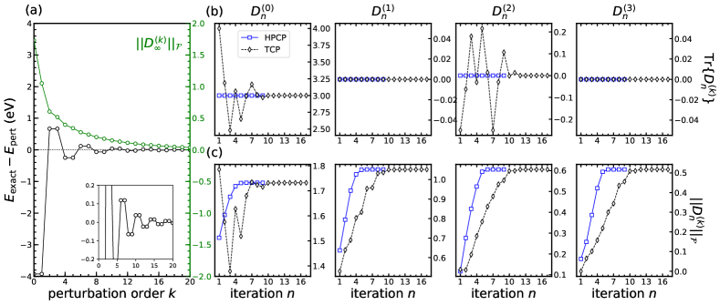
Figure 1: Perturbation series for $\pi$-bonding in benzene using perturbed Hückel matrices (see text for details). (a) Convergence of the perturbed energy and Frobenius norm of the corresponding perturbed density matrices using purification-DMPT. The convergence of the unperturbed and firsts 3 perturbed density matrices during the purification cycles are presented in terms of their traces (b), and their norms (c), for both the TC2 and HPCP polynomials.

In both examples, the perturbation series is expected to converge such that, by setting $\lambda=1$, the sum over the perturbed densities in Eq. (12a) converges towards the exact density matrix $D_{\lambda}$ as obtained from the full Hamiltonian $H_{\lambda}$ ; obtained for instance by diagonalizing $H_{\lambda}$ and summing over the $N$ occupied states as in Eq. (4). The same way, the sum over the perturbed energies, $E_{\textrm{pert}}=\sum_{k}E^{(k)}$, computed from Eq. (16) must converge towards the exact reference value, $E_{\textrm{exact}}=2\textrm{Tr}\{H_{\lambda}D_{\lambda}\}$. This is demonstrated for benzene and pyridine in Figs. 1(a) and 2(a), respectively, where $E_{\textrm{exact}}-E_{\textrm{pert}}$ are plotted as a function of the number of perturbation terms entering in $\sum_{k}E^{(k)}$, up to $k=20$. For benzene, we note that for symmetry reason only even orders contribute to $E_{\textrm{pert}}$. At $k=20$, for benzene, we found that $E_{\textrm{pert}}$ is converged to within 5 meV for $E_{\textrm{exact}}=-88.9440$ eV, compared to a much faster convergence for pyridine with the same level of convergence reach at $k=3$, with $E_{\textrm{exact}}=-85.1005$ eV. On the same figures ($y$-right axis) are also reported the norms of the density matrices $||D_{\infty}^{(k)}||$ as a function of $k$ which confirm the faster convergence of the $\pi$-bonding perturbation in pyridine.

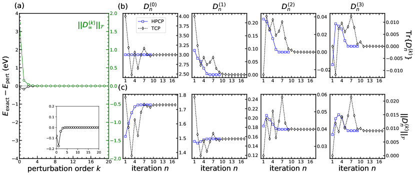
Figure 2: Perturbation series for $\pi$-bonding in pyridine (see text for details). (a) Convergence of the perturbed energy and Frobenius norm of the corresponding perturbed density matrices using purification-DMPT. The convergence of the unperturbed and firsts 3 perturbed density matrices during the purification cycles are presented in terms of their traces (b), and their norms (c), for both the TC2 and HPCP polynomials.

We emphasize that identical results were obtained with the reference McWeeny- and Sylvester-DMPT. Considering the benzene perturbation series at higher order, reliability of the purification-based DMPT starts to degrade for $k>55$ using HPCP compared to $k>17$ for TC2. This trend has been confirmed for other systems and $\pi$-bonding perturbations (not shown here), indicating that the HPCP purification is more stable than TC2 when increasing the perturbation order. This could be related to the ill-definition of the stopping criteria of TC2, becoming a very sensitive parameter in the extreme conditions of very high perturbation order. Nevertheless, this has a weak interest in practical applications since they generally do not require a perturbed density matrix higher than the order 3.

Evolution of the density matrices (up to the order 3) during the purification process are plotted on Figs. 1 and 2, panels (b) for the trace and (c) for the norm. First, in both cases, the convergence of the HPCP-DMPT is achieved in fewer iterations compared to TC2 as expected from the convergence profile of the two polynomials (quadratic vs. linear, respectively). The property of trace-conservation of the zero-order density matrix fulfilled by the HPCP is apparent from these figures. In this respect, the TC2 polynomial demonstrates an erratic behavior with strong oscillations at the beginning of the purification. These oscillations remain present at higher order, especially when looking to the pyridine case. We note that the zero-trace conservation of $D^{(1)}$ and $D^{(3)}$ observed with both polynomials for the case of benzene should not be overinterpreted since they are merely related to symmetry of the system. As a matter of fact, for the more general case of pyridine, such property of zero-trace conservation is not observed. Overall, the convergence behavior of the HPCP polynomials is more smooth than TC2 with, after the first few steps a quasi systematic monotonic approach of the converged perturbed density matrix.

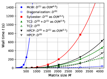
Figure 3: Scaling performance for the various methods to obtain $D^{(0)}$ and $D^{(1)}$ using a benchmark of Hückel matrices of increasing size. Non-linear fits of equation $t=\alpha M^{\beta}$ are plotted with solid lines.

In order to compare the computational performances of the purification, McWeeny and Sylvester DMPT we have performed a set of calculations on systems of increasing size. As for the pyridine case, unperturbed Hückel matrices for aromatic hydrocarbons with increasing ring size were generated along with first-order perturbed Hamiltonians describing the substitution of one of the carbon by a nitrogen atom. On Fig. 3 is plotted the CPU time spent to obtain the unperturbed and first-order perturbed density matrices with respect to the size of the Hückel matrix. The same tolerence parameter of $||D_{n+1}-D_{n}||_{\mathcal{F}}<10^{-12}$ was used for purifications. We emphasize here that the McWeeny and Sylveter-DMPT are direct methods such that provided the eigenstates (or only the unperturbed density matrix for Sylveter-DMPT), the number of FLOPS to solve the DMPT equations is fixed by the size of the problem $M$, whereas for purification-based methods the solutions are found iteratively. In this case the number of iterations depends on the band-gap of the system,Niklasson (2002); Rudberg and Rubensson (2011) and for HPCP, to a lesser extent, on the filling factor $\theta$.Truflandier, Dianzinga, and Bowler (2016) In our example, ideal conditions are fulfilled to minimize the number of purifications with $\theta=1/2$ and a large HOMO-LUMO gap when compared to the range of the full eigenspectrum. Note that the size of the N-substituted aromatic hydrocarbons does not impact the HOMO-LUMO gap, for which we found, as for pyridine, that the density matrices are converged after 9 and 17 purifications for HPCP and TC2, respectively, independently of $M$. From Fig. 3, we note that exact diagonalization is more efficient than the purification methods to obtain the unperturbed density matrix. However, once we consider the perturbed state, we observe a net benefit to solve the Sylvester-DMPT equations using the Bartels-Stewart algorithm compare to the sum-over-states approach of McWeeny, which are expected to scales as $O(M^{4})$ and $O(M^{3})$, respectively. Note that the effective scaling reported on Fig. 3 are in good agreement with these expectations. If now we consider purification methods, which also scales as $O(M^{3})$, the computational performances are further improved. We stress that for very low band gaps these performances are expected to degrade with a CPU time multiplied by a factor 5 at worst.Truflandier, Dianzinga, and Bowler (2016) Finally, it should be mentioned that for purification-DMPT the plots of Fig. 3 incorporate the calculation time for both $D^{(0)}$ and $D^{(1)}$ (since they cannot be decoupled), whereas for direct methods the former has not been included, increasing the interest for the TC2/HPCP DMPT. Comparison of the TC2 and HPCP shows that despite the more rapid convergence of HPCP, the TC2 presents better performances due to its lower number of MMs which is always (independently of the perturbation order) more than twice less than the one of HPCP. Typically in our example, TC2 requires 2 MMs per iteration compared to 5 for HPCP. However HPCP requires twice less iterations.

IV Conclusions and perspectives

In this work, we have reviewed three types of density matrix perturbation theory with, for two of them, a resolution of the perturbed density matrices without the support of the unperturbed eigenstates. These two methods, namely the Sylvester- and purification-DMPT, clearly demonstrate better computational performances compared to the standard sum-over-states approach. This indicates that current response equation solver as implemented in quantum chemistry codes can be significantly accelerated using those two methods. We have also sucessfully extended the recursive DMPT proposed by Niklasson and Challacombe to the HPCP polynomial. Compared to TC2, the HPCP-DMPT shows a better stability when approaching convergence, but remains more expensive in terms of computational performance. We emphasize that, in favorable conditions, i.e. for insulators with a filling factor around 1/2, the TCP/HPCP-DMPT clearly outperforms the other approaches. In the near future, we plan to implement the Sylvester- and purification-DMPT using non-orthogonal and perturbation dependent basis set.Niklasson, Weber, and Challacombe (2005); Niklasson and Weber (2007) Within the framework of linear scaling density functional theory as implemented in the CONQUEST code,Nakata et al. (2020) this will allow for application to electric and magnetic response calculations at a linear scaling computational cost.

V Data availability

The data that support the findings of this study are available from the corresponding author upon reasonable request

Appendix A SOS-McWeeny DMPT: 2nd and 3rd orders

The second-order equation can be derived by applying the resolution of identity to both side of Eq. (13c). Conserving notations of Eq. (17), we obtain

$$2D_{oo}^{(2)}+D_{ov}^{(2)}+D_{vo}^{(2)} +(D^{(1)}D^{(1)})_{oo}+(D^{(1)}D^{(1)})_{vv}$$

$$\cdots +(D^{(1)}D^{(1)})_{ov}+(D^{(1)}D^{(1)})_{vo}$$

$$=D_{oo}^{(2)} +D_{ov}^{(2)}+D_{vo}^{(2)}+D_{vv}^{(2)}$$ (77)

By resolving the product of first-order perturbed density matrices according to

$$D^{(1)}D^{(1)} =D^{(1)}ID^{(1)}$$

$$=D^{(1)}(D+\bar{D})D^{(1)}$$

$$=D^{(1)}(D^{2}+\bar{D}^{2})D^{(1)}$$

we obtain

$$(D^{(1)}D^{(1)})_{oo} =D_{oo}^{(1)}D_{oo}^{(1)}+D_{ov}^{(1)}D_{vo}^{(1)}$$ (78a)

$$(D^{(1)}D^{(1)})_{vv} =D_{vv}^{(1)}D_{vv}^{(1)}+D_{vo}^{(1)}D_{ov}^{(1)}$$ (78b)

$$(D^{(1)}D^{(1)})_{ov} =D_{ov}^{(1)}D_{vv}^{(1)}+D_{oo}^{(1)}D_{ov}^{(1)}$$ (78c)

$$(D^{(1)}D^{(1)})_{vo} =D_{vo}^{(1)}D_{oo}^{(1)}+D_{vv}^{(1)}D_{vo}^{(1)}$$ (78d)

On inserting the rhs of Eqs. (78) into (77), and using the properties of Eq. (19), we have

$$2D_{oo}^{(2)}+D_{ov}^{(2)} +D_{vo}^{(2)}+D_{ov}^{(1)}D_{vo}^{(1)}+D_{vo}^{(1)}D_{ov}^{(1)}$$

$$=D_{oo}^{(2)}+D_{ov}^{(2)}+D_{vo}^{(2)}+D_{vv}^{(2)}$$ (79)

Therefore, we find

$$D_{oo}^{(2)} =-D_{ov}^{(1)}D_{vo}^{(1)}$$ (80a)

$$D_{vv}^{(2)} =+D_{vo}^{(1)}D_{ov}^{(1)}$$ (80b)

Unlike the 1st-order perturbation, the diagonal components of the 2nd-order perturbed density matrix are likely to be non-zero and can be computed from the 1st-order perturbed density matrix. Relying furthermore on the symmetry of the perturbed density, it leaves only the occupied-virtual coupling block matrix to evaluate. On resolving the 2nd-order perturbed Hamiltonian matrix using Eq. (14c), we obtain

$$H_{ov}^{(2)}=[H,D_{ov}^{(2)}]+[H^{(1)},D^{(1)}]_{ov}$$ (81)

Using the spectral resolution of the non-perturbed Hamiltonian matrix and the perturbed density matrix, Eq. (81) transforms as

$$H_{ov}^{(2)}=\sum_{i,j}\left(D_{ov,ij}^{(2)}(\epsilon_{i}-\bar{\epsilon}_{j})+[H^{(1)},D^{(1)}]_{ov,ij}\right)$$ (82)

which leads to

$$D_{ov}^{(2)}=\sum_{i,j}(\epsilon_{i}-\bar{\epsilon}_{j})^{-1}\left(H_{ov}^{(2)}-[H^{(1)},D^{(1)}]_{ov}\right)_{ij}$$ (83)

The final 2nd-order perturbed density matrix is obtained by summing over $D_{ov}^{(2)}$, its conjugate-transposed and the block-diagonal contributions of Eq. (80).

Using the same route, the third-order response equation can be derived from Eq. (13d). This yields to

$$2D_{oo}^{(3)}+D_{ov}^{(3)}+D_{vo}^{(3)} +(D^{(1)}D^{(2)})_{oo}+(D^{(1)}D^{(2)})_{vv}$$

$$\cdots +(D^{(1)}D^{(2)})_{ov}+(D^{(1)}D^{(2)})_{vo}$$

$$\cdots +(D^{(2)}D^{(1)})_{oo}+(D^{(2)}D^{(1)})_{vv}$$

$$\cdots +(D^{(2)}D^{(1)})_{ov}+(D^{(2)}D^{(1)})_{vo}$$

$$=D_{oo}^{(3)} +D_{ov}^{(3)}+D_{vo}^{(3)}+D_{vv}^{(3)}$$ (84)

where

$$(D^{(1)}D^{(2)})_{oo}=D_{oo}^{(1)}D_{oo}^{(2)}+D_{ov}^{(1)}D_{vo}^{(2)}$$ (85a)

$$(D^{(1)}D^{(2)})_{vv}=D_{vv}^{(1)}D_{vv}^{(2)}+D_{vo}^{(1)}D_{ov}^{(2)}$$ (85b)

$$(D^{(1)}D^{(2)})_{ov}=D_{ov}^{(1)}D_{vv}^{(2)}+D_{oo}^{(1)}D_{ov}^{(2)}$$ (85c)

$$(D^{(1)}D^{(2)})_{vo}=D_{vo}^{(1)}D_{oo}^{(2)}+D_{vv}^{(1)}D_{vo}^{(2)}$$ (85d)

$$(D^{(2)}D^{(1)})_{oo}=D_{oo}^{(2)}D_{oo}^{(1)}+D_{ov}^{(2)}D_{vo}^{(1)}$$ (85e)

$$(D^{(2)}D^{(1)})_{vv}=D_{vv}^{(2)}D_{vv}^{(1)}+D_{vo}^{(2)}D_{ov}^{(1)}$$ (85f)

$$(D^{(2)}D^{(1)})_{ov}=D_{ov}^{(2)}D_{vv}^{(1)}+D_{oo}^{(2)}D_{ov}^{(1)}$$ (85g)

$$(D^{(2)}D^{(1)})_{vo}=D_{vo}^{(2)}D_{oo}^{(1)}+D_{vv}^{(2)}D_{vo}^{(1)}$$ (85h)

From Eqs. (19), (80) and (85), Eq. (84) simplifies to

$$2D_{oo}^{(3)}+D_{ov}^{(3)}+D_{vo}^{(3)} +D_{ov}^{(1)}D_{vo}^{(2)}+D_{ov}^{(2)}D_{vo}^{(1)}$$

$$\cdots +D_{vo}^{(1)}D_{ov}^{(2)}+D_{vo}^{(2)}D_{ov}^{(1)}$$

$$=D_{oo}^{(3)} +D_{ov}^{(3)}+D_{vo}^{(3)}+D_{vv}^{(3)}$$ (86)

On identifying lhs and rhs terms, it follows that

$$D_{oo}^{(3)} =-\left(D_{ov}^{(1)}D_{vo}^{(2)}+D_{ov}^{(2)}D_{vo}^{(1)}\right)$$ (87a)

$$D_{vv}^{(3)} =+\left(D_{vo}^{(1)}D_{ov}^{(2)}+D_{vo}^{(2)}D_{ov}^{(1)}\right)$$ (87b)

Again, the last equation shows that the diagonal components are computed with the 1st and 2nd-order perturbed density matrices. At this point, we emphasize that only the occupied-virtual transition matrix needs to be evaluated since the perturbed density matrix is Hermitian.

Relying on the spectral resolution, the 3rd-order perturbed Hamiltonian matrix is given by

$$H_{ov}^{(3)} =[H,D_{ov}^{(3)}]+[H^{(1)},D^{(2)}]_{ov}+[H^{(2)}D^{(1)}]_{ov}$$ (88a)

$$=\sum_{i,j}D_{ov,ij}^{(3)}(\epsilon_{i}-\bar{\epsilon}_{j})$$

$$\times\left([H^{(1)},D^{(2)}]_{ov}+[H^{(2)}D^{(1)}]_{ov}\right)_{ij}$$ (88b)

which leads to

$$D_{ov}^{(3)} =\sum_{i,j}(\epsilon_{i}-\bar{\epsilon}_{j})^{-1}$$

$$\times\left(H_{ov}^{(3)}-[H^{(1)},D^{(2)}]_{ov}-[H^{(2)},D^{(1)}]_{ov}\right)_{ij}$$ (89)

By summing over contributions of Eqs. (87) and (89) and its conjugate-transposed, we obtain the 3rd-order perturbed density matrix. It is worth mentioning that the direct resolutions of the 2nd or 3rd-order perturbed quantities implies prior knowledge of the lower orders (1st and 2nd, respectively), in such a way that, whatever is the order to be resolved, i.e. Eqs. (87)–(89) on one side, or Eqs. (80)–(83) on the other side, both cases involve to solve for the linear-response of the order $(k-1)$ to obtain the perturbed quantities at the order $k$. Eventually, by mathematical induction it is straightforward to generalize these working equations to any order $k$, as introduced in Eqs. (27)–(31).

Appendix B Alternative formulation of DMPT

In this appendix, we shall show that the planewave-based DMPT introduced by Lazzeri and MauriLazzeri and Mauri (2003b) is closely related to the atomic-orbital based DMPT method of Kussmann and OchsenfeldKussmann and Ochsenfeld (2007a, b), (and by extension the Sylvester-DMPT) both relying on the CG minimization. Thereafter, they will be referred to as PW-DMPT and AO-DMPT, respectively.

As discussed in Section II.4, employing a PW basis set with $M_{\textrm{PW}}>>N$ constrains us to use iterative diagonalization, where, for an insulator, the $N$ first (lowest) eigenstates, $\{\epsilon_{i},\psi_{i}\}^{N}_{i\in\textrm{occ}}$, necessary and sufficient to obtain the unperturbed ground-state, can be determined with a satisfying accuracy. Here, we will assume the linear-DMPT regime: in order to determine the $k$th-order perturbed density, all the preceding orders, up to $(k-1)$, are known. As a result, for a PW basis set, at the zero order, the unperturbed density matrix, $D^{(0)}\equiv D$, can be resolved in terms of the occupied states following Eq. (4), and knowing only the occupied eigenstates, the unperturbed Hamiltonian matrix, $H^{(0)}\equiv H$, can be formally expressed as:

$$H=\sum_{i\in\textrm{occ}}|\psi_{i}\rangle\epsilon_{i}\langle\psi_{i}|+\bar{D}H\bar{D}$$ (90)

recalling that, from the closure relation of Eq. (9), $\bar{D}=I-D$. Within the framework of the AO-DMPT method, the $k$-order perturbed density matrix, $D^{(k)}$, is found as solution of the following equation:

$$[D,\sum^{k}_{l=0}[H^{(l)},D^{(k-l)}]]=0$$ (91)

It must be emphasized that, in comparison to the McWeeny-DMPT and Eq. (22), or the PW-DMPT and Eq. (90), the resolution of the AO-DMPT equation is free of any intermediate spectral resolution of the unperturbed Hamiltonian matrix. Indeed, the PW-DMPT may be view as an intermediate strategy, between the former and the later, where Eq. (91) is decomposed to perform an occupied-perturbed state-by-state resolution.Lazzeri and Mauri (2003b) For instance, on applying to Eq. (91) the identity: $[D,O]=DO\bar{D}-\bar{D}OD$, and projecting to the right on $|\psi_{i}\rangle$ with $i\in\textrm{occ}$, we find:

$$\bar{D}\sum^{k}_{l=0}[H^{(l)},D^{(k-l)}]|\psi_{i}\rangle=0$$ (92)

By extracting the terms containing the $k$th-order density matrix from the sum, and by reordering, it appears:

$$\left(\bar{D}HD^{(k)}-\bar{D}D^{(k)}H\right)|\psi_{i}\rangle=-\sum^{k}_{l=1}\bar{D}[H^{(l)},D^{(k-l)}]|\psi_{i}\rangle$$ (93)

On substitution of the expression of $H$ from Eq. (90) into Eq. (93), and recalling that, at the zero temperature limit, the converged ground-state one-electron and one-hole density matrices must respect the idempotency and the stationary conditions of Eqs. (13a) and (14a), respectively, we arrive at:

$$\left(H\bar{D}D^{(k)}-\bar{D}D^{(k)}\epsilon_{i}\right)|\psi_{i}\rangle=-\sum^{k}_{l=1}\bar{D}[H^{(l)},D^{(k-l)}]|\psi_{i}\rangle$$ (94)

Complying with notations of Ref. [​​69] by introducing,

$$|\eta^{(k)}_{i}\rangle =\bar{D}D^{(k)}|\psi_{i}\rangle$$ (95a)

$$\textrm{such that}\quad D_{vo}^{(k)} =\sum_{i\in\textrm{occ}}|\eta^{(k)}_{i}\rangle\langle\psi_{i}|$$ (95b)

we recover Eq. (13) of the article, that is,

$$\left(H-I\epsilon_{i}\right)|\eta^{(k)}_{i}\rangle=-\sum^{k}_{l=1}\bar{D}[H^{(l)},D^{(k-l)}]|\psi_{i}\rangle$$ (96)

In the interests of completeness, the SOS equation (29) can be found back by further resolving the full spectrum of $H$. By using Eq. (22), along with the resolution of identity (9), the lhs of Eq. (96) transforms as

$$\left(H-\epsilon_{i}I\right)|\eta^{(k)}_{i}\rangle =\sum_{i^{\prime}\in\textrm{occ}}|\psi_{i^{\prime}}\rangle(\epsilon_{i^{\prime}}-\epsilon_{i})\langle\psi_{i^{\prime}}|\eta^{(k)}_{i}\rangle$$

$$+\sum_{j^{\prime}\in\textrm{virt}}|\bar{\psi}_{j^{\prime}}\rangle(\bar{\epsilon}_{j^{\prime}}-\epsilon_{i})\langle\bar{\psi}_{j^{\prime}}|\eta^{(k)}_{i}\rangle$$ (97)

By remarking that: (i) $\langle\psi_{i^{\prime}}|\eta^{(k)}_{i}\rangle=0$ $\forall i^{\prime}$, and (ii) $\langle\bar{\psi}_{j^{\prime}}|\eta^{(k)}_{i}\rangle=\langle\bar{\psi}_{j^{\prime}}|D^{(k)}|\psi_{i}\rangle$, we found that Eq. (97) simplifies to

$$\left(H-\epsilon_{i}I\right)|\eta^{(k)}_{i}\rangle=\sum_{j\in\textrm{virt}}|\bar{\psi}_{j}\rangle(\bar{\epsilon}_{j}-\epsilon_{i})\langle\bar{\psi}_{j}|D^{(k)}|\psi_{i}\rangle$$ (98)

Inserted in the lhs of Eq. (96) and resolving the one-hole density matrix of the rhs, we have

$$\sum_{j\in\textrm{virt}} (\bar{\epsilon}_{j}-\epsilon_{i})|\bar{\psi}_{j}\rangle\langle\bar{\psi}_{j}|D^{(k)}|\psi_{i}\rangle$$

$$=\sum^{k}_{l=1}\sum_{j\in\textrm{virt}}|\bar{\psi}_{j}\rangle\langle\bar{\psi}_{j}|[D^{(k-l)},H^{(l)}]|\psi_{i}\rangle$$ (99)

which further gives the analytical expression of $|\eta^{(k)}_{i}\rangle$ with respect to the lower order perturbed density matrices,

$$|\eta^{(k)}_{i}\rangle=\sum^{k}_{l=1}\sum_{j\in\textrm{virt}}\frac{\langle\bar{\psi}_{j}|[D^{(k-l)},H^{(l)}]|\psi_{i}\rangle}{\bar{\epsilon}_{j}-\epsilon_{i}}|\bar{\psi}_{j}\rangle$$ (100)

Following definitions (95), by summing over the $N$ perturbed projectors, this yields to the $k$th virtual-occupied transition matrix,

$$D_{vo}^{(k)}=\sum^{k}_{l=1}\sum_{i\in\textrm{occ}}\sum_{j\in\textrm{virt}}\frac{\langle\bar{\psi}_{j}|[D^{(k-l)},H^{(l)}]|\psi_{i}\rangle}{\bar{\epsilon}_{j}-\epsilon_{i}}|\bar{\psi}_{j}\rangle\langle\psi_{i}|$$ (101)

which is the conjugate transpose of the McWeeny equation (29). Note that, for $k>1$, the remaining occupied-occupied and virtual-virtual components necessary to build the full $k$th-order matrix, i.e. $D^{(k)}=D_{ov}^{(k)}+D_{vo}^{(k)}+D_{oo}^{(k)}+D_{vv}^{(k)}$, can be easily computed from the lowest orders using Eqs. (30) and (31).

References

- Weiße et al. (2006) A. Weiße, G. Wellein, A. Alvermann, and H. Fehske, Rev. Mod. Phys. 78, 275 (2006).
- Stevens, Pitzer, and Lipscomb (1963) R. M. Stevens, R. M. Pitzer, and W. N. Lipscomb, J. Chem. Phys. 38, 550 (1963).
- Gerratt and Mills (1968a) J. Gerratt and I. M. Mills, J. Chem. Phys. 49, 1719 (1968a).
- Gerratt and Mills (1968b) J. Gerratt and I. M. Mills, J. Chem. Phys. 49, 1730 (1968b).
- Thomsen and Swanstrøm (1973) K. Thomsen and P. Swanstrøm, Mol. Phys. 26, 735 (1973).
- Ditchfield (1974) R. Ditchfield, Mol. Phys. 27, 789 (1974).
- Pople et al. (1979) J. A. Pople, R. Krishnan, H. B. Schlegel, and J. S. Binkley, Int. J. Quantum Chem. 16, 225 (1979).
- Frisch, Head-Gordon, and Pople (1990) M. Frisch, M. Head-Gordon, and J. Pople, Chem. Phys. 141, 189 (1990).
- Osamura et al. (1983) Y. Osamura, Y. Yamaguchi, P. Saxe, D. J. Fox, M. A. Vincent, and H. F. Schaefer, J. Mol. Struct.: THEOCHEM 103, 183 (1983).
- McWeeny (1962) R. McWeeny, Phys. Rev. 126, 1028 (1962).
- McWeeny (1968) R. McWeeny, Chem. Phys. Lett. 1, 567 (1968).
- Diercksen and McWeeny (1966) G. Diercksen and R. McWeeny, J. Chem. Phys. 44, 3554 (1966).
- Pople (1953) J. A. Pople, Trans. Faraday Soc. 49, 1375 (1953).
- Pariser and Parr (1953a) R. Pariser and R. G. Parr, J. Chem. Phys. 21, 767 (1953a).
- Pariser and Parr (1953b) R. Pariser and R. G. Parr, J. Chem. Phys. 21, 466 (1953b).
- Moccia (1967) R. Moccia, Theoret. Chim. Acta 8, 192 (1967).
- Moccia (1970) R. Moccia, Chem. Phys. Lett. 5, 260 (1970).
- Dodds, McWeeny, and Sadlej (1977) J. L. Dodds, R. McWeeny, and A. J. Sadlej, Mol. Phys. 34, 1779 (1977).
- Dodds et al. (1977) J. L. Dodds, R. McWeeny, W. T. Raynes, and J. P. Riley, Mol. Phys. 33, 611 (1977).
- Woliński and Sadlej (1980) K. Woliński and A. J. Sadlej, Mol. Phys. 41, 1419 (1980).
- Woliński, Hinton, and Pulay (1990) K. Woliński, J. F. Hinton, and P. Pulay, J. Am. Chem. Soc. 112, 8251 (1990).
- Ochsenfeld and Head-Gordon (1997) C. Ochsenfeld and M. Head-Gordon, Chem. Phys. Lett. 270, 399 (1997).
- Li, Nunes, and Vanderbilt (1993) X.-P. Li, R. W. Nunes, and D. Vanderbilt, Phys. Rev. B 47, 10891 (1993).
- McWeeny (1956) R. McWeeny, Proc. R. Soc. Lond. A 235, 496 (1956).
- McWeeny (1960) R. McWeeny, Rev. Mod. Phys. 32, 335 (1960).
- Kussmann and Ochsenfeld (2007a) J. Kussmann and C. Ochsenfeld, J. Chem. Phys. 127, 054103 (2007a).
- Kussmann and Ochsenfeld (2007b) J. Kussmann and C. Ochsenfeld, J. Chem. Phys. 127, 204103 (2007b).
- Larsen et al. (2001) H. Larsen, T. Helgaker, J. Olsen, and P. Jørgensen, J. Chem. Phys. 115, 10344 (2001).
- Coriani et al. (2007) S. Coriani, S. Høst, B. Jansík, L. Thøgersen, J. Olsen, P. Jørgensen, S. Reine, F. Pawłowski, T. Helgaker, and P. Sałek, J. Chem. Phys. 126, 154108 (2007).
- Helgaker et al. (2000) T. Helgaker, H. Larsen, J. Olsen, and P. Jørgensen, Chem. Phys. Lett. 327, 397 (2000).
- Niklasson and Challacombe (2004) A. M. N. Niklasson and M. Challacombe, Phys. Rev. Lett. 92, 193001 (2004).
- Niklasson, Weber, and Challacombe (2005) A. M. N. Niklasson, V. Weber, and M. Challacombe, J. Chem. Phys. 123, 044107 (2005).
- Niklasson and Weber (2007) A. M. N. Niklasson and V. Weber, J. Chem. Phys. 127, 064105 (2007).
- Niklasson (2002) A. M. N. Niklasson, Phys. Rev. B 66, 155115 (2002).
- Cawkwell et al. (2012) M. J. Cawkwell, E. J. Sanville, S. M. Mniszewski, and A. M. N. Niklasson, J. Chem. Theory Comput. 8, 4094 (2012).
- Cawkwell et al. (2014) M. J. Cawkwell, M. A. Wood, A. M. N. Niklasson, and S. M. Mniszewski, J. Chem. Theory Comput. 10, 5391 (2014).
- Weber, Niklasson, and Challacombe (2004) V. Weber, A. M. N. Niklasson, and M. Challacombe, Phys. Rev. Lett. 92, 193002 (2004).
- Weber, Niklasson, and Challacombe (2005) V. Weber, A. M. N. Niklasson, and M. Challacombe, J. Chem. Phys. 123, 044106 (2005).
- Truflandier, Dianzinga, and Bowler (2016) L. A. Truflandier, R. M. Dianzinga, and D. R. Bowler, J. Chem. Phys. 144, 091102 (2016).
- Goedecker and Teter (1995) S. Goedecker and M. Teter, Phys. Rev. B 51, 9455 (1995).
- Baer and Head-Gordon (1997) R. Baer and M. Head-Gordon, Phys. Rev. Lett. 79, 3962 (1997).
- Hirschfelder, Brown, and Epstein (1964) J. O. Hirschfelder, W. B. Brown, and S. T. Epstein, in Advances in Quantum Chemistry, Vol. 1 (Elsevier, 1964) pp. 255–374.
- Helgaker, Jørgensen, and Olsen (2000) T. Helgaker, P. Jørgensen, and J. Olsen, Molecular Electronic-Structure Theory (John Wiley & Sons, Ltd, London, 2000).
- Pulay (1983) P. Pulay, J. Chem. Phys. 78, 5043 (1983).
- Sekino and Bartlett (1986) H. Sekino and R. J. Bartlett, J Chem. Phys. 85, 976 (1986).
- Karna and Dupuis (1991) S. P. Karna and M. Dupuis, J. Comput. Chem. 12, 487 (1991).
- Furche (2001) F. Furche, J. Chem. Phys. 114, 5982 (2001).
- Kobayashi, Touma, and Nakai (2012) M. Kobayashi, T. Touma, and H. Nakai, J. Chem. Phys. 136, 084108 (2012).
- Kußmann (2006) J. Kußmann (Universität Tübingen, Germany, 2006).
- Note (1) The passing from to Eq. (32) required the use of the identity: .
- Brandts (2001) J. Brandts, in Large-Scale Scientific Computing, edited by S. Margenov, J. Waśniewski, and P. Yalamov (Springer Berlin Heidelberg, Berlin, Heidelberg, 2001) pp. 462–470.
- Simoncini (2016) V. Simoncini, SIAM Rev. 58, 377 (2016).
- Note (2) Note that the special case where in the Sylvester equation is also referred to as the Lyapunov equation in litteratureSimoncini (2016).
- Bartels and Stewart (1972) R. H. Bartels and G. W. Stewart, Commun. ACM 15, 820 (1972).
- Saad (2003) Y. Saad, Iterative Methods for Sparse Linear Systems, Other Titles in Applied Mathematics (Society for Industrial and Applied Mathematics, 2003).
- Nocedal and Wright (2006) J. Nocedal and S. Wright, Numerical Optimization, 2nd ed., Springer Series in Operations Research and Financial Engineering (Springer-Verlag, New York, 2006).
- Davidson (1975) E. R. Davidson, J. Comput. Phys. 17, 87 (1975).
- Wood and Zunger (1985) D. M. Wood and A. Zunger, J. Phys. A: Math. Gen. 18, 1343 (1985).
- Kresse and Furthmüller (1996a) G. Kresse and J. Furthmüller, Phys. Rev. B 54, 11169 (1996a).
- Teter, Payne, and Allan (1989) M. P. Teter, M. C. Payne, and D. C. Allan, Phys. Rev. B 40, 12255 (1989).
- Payne et al. (1992) M. C. Payne, M. P. Teter, D. C. Allan, T. A. Arias, and J. D. Joannopoulos, Rev. Mod. Phys. 64, 1045 (1992).
- Giannozzi et al. (2009) P. Giannozzi, S. Baroni, N. Bonini, M. Calandra, R. Car, C. Cavazzoni, D. Ceresoli, G. L. Chiarotti, M. Cococcioni, I. Dabo, A. Dal Corso, S. de Gironcoli, S. Fabris, G. Fratesi, R. Gebauer, U. Gerstmann, C. Gougoussis, A. Kokalj, M. Lazzeri, L. Martin-Samos, N. Marzari, F. Mauri, R. Mazzarello, S. Paolini, A. Pasquarello, L. Paulatto, C. Sbraccia, S. Scandolo, G. Sclauzero, A. P. Seitsonen, A. Smogunov, P. Umari, and R. M. Wentzcovitch, J. Phys.: Condensed Matt. 21, 395502 (2009).
- Kresse and Furthmüller (1996b) G. Kresse and J. Furthmüller, Comput. Mater. Sci. 6, 15 (1996b).
- Gonze (1995) X. Gonze, Phys. Rev. A 52, 1096 (1995).
- Gonze (1997) X. Gonze, Phys. Rev. B 55, 10337 (1997).
- Baroni, Giannozzi, and Testa (1987) S. Baroni, P. Giannozzi, and A. Testa, Phys. Rev. Lett. 58, 1861 (1987).
- Baroni et al. (2001) S. Baroni, S. de Gironcoli, A. Dal Corso, and P. Giannozzi, Rev. Mod. Phys. 73, 515 (2001).
- Lazzeri and Mauri (2003a) M. Lazzeri and F. Mauri, Phys. Rev. Lett. 90, 036401 (2003a).
- Lazzeri and Mauri (2003b) M. Lazzeri and F. Mauri, Phys. Rev. B 68, 161101 (2003b).
- Niklasson (2011) A. M. N. Niklasson, in Linear-Scaling Techniques in Computational Chemistry and Physics, Challenges and Advances in Computational Chemistry and Physics No. 13, edited by R. Zalesny, M. G. Papadopoulos, P. G. Mezey, and J. Leszczynski (Springer Netherlands, 2011) pp. 439–473.
- Geršgorin (1931) S. Geršgorin, Proc. USSR Acad. Sci. 51, 749 (1931).
- Note (3) Even if obvious, we recall that: . The TC2 formulation of Eq. (40a) using instead of the is only useful when compared with the HPCP polynomial (43).
- Rubensson (2012) E. Rubensson, SIAM J. Sci. Comput. 34, B1 (2012).
- Rubensson, Rudberg, and Sałek (2008) E. H. Rubensson, E. Rudberg, and P. Sałek, J. Chem. Phys. 128, 074106 (2008).
- Palser and Manolopoulos (1998) A. H. R. Palser and D. E. Manolopoulos, Phys. Rev. B 58, 12704 (1998).
- Mazziotti (2003) D. A. Mazziotti, Phys. Rev. E 68, 066701 (2003).
- Note (4) Maybe it is worth to recall that for square matrices of size , the number of floating-point operations (FLOPs) for dense matrix-matrix multiplication scales as , compare to for all the other matrix operations involved in those perturbed recursions, e.g. scalar multiplication, addition and transposition.
- Note (5) For odd, exactly MMs must be performed for the TC2 vs. for the HPCP. For even, it is found vs. MMs, respectively.
- Albright, Burdett, and Whangbo (1985) T. A. Albright, J. K. Burdett, and M. Whangbo, Orbital Interactions in Chemistry (John Wiley & Sons, Ltd, 1985).
- Rudberg and Rubensson (2011) E. Rudberg and E. H. Rubensson, J. Phys.: Condens. Matter 23, 075502 (2011).
- Nakata et al. (2020) A. Nakata, J. S. Baker, S. Y. Mujahed, J. T. L. Poulton, S. Arapan, J. Lin, Z. Raza, S. Yadav, L. Truflandier, T. Miyazaki, and D. R. Bowler, J. Chem. Phys. 152, 164112 (2020), https://doi.org/10.1063/5.0005074 .