A Study of Gradient Variance in Deep Learning

Abstract

The impact of gradient noise on training deep models is widely acknowledged but not well understood. In this context, we study the distribution of gradients during training. We introduce a method, Gradient Clustering, to minimize the variance of average mini-batch gradient with stratified sampling. We prove that the variance of average mini-batch gradient is minimized if the elements are sampled from a weighted clustering in the gradient space. We measure the gradient variance on common deep learning benchmarks and observe that, contrary to common assumptions, gradient variance increases during training, and smaller learning rates coincide with higher variance. In addition, we introduce normalized gradient variance as a statistic that better correlates with the speed of convergence compared to gradient variance.

1 Introduction

Many machine learning tasks entail the minimization of the risk, ${\mathbb{E}}_{\bm{x}}[\ell(\bm{x};{\bm{\theta}})]$, where $\bm{x}$ is an i.i.d. sample from a data distribution, and $\ell$ is the per-example loss parametrized by ${\bm{\theta}}$. In supervised learning, inputs and ground-truth labels comprise $\bm{x}$, and ${\bm{\theta}}$ is a vector of model parameters. Empirical risk approximates the population risk by the risk of a sample set $\{{\bm{x}_{i}}\}_{i=1}^{N}$, the training set, as $L({\bm{\theta}})={\sum_{i=1}^{N}}\ell({\bm{x}_{i}};{\bm{\theta}})/N$. Empirical risk is often minimized using gradient-based optimization (first-order methods). For differentiable loss functions, the gradient of $\bm{x}$ is defined as ${\frac{\partial{}}{\partial\theta}}\ell(\bm{x};{\bm{\theta}})$, i.e. the gradient of the loss with respect to the parameters evaluated at a point $\bm{x}$. Popular in deep learning, Mini-batch Stochastic Gradient Descent (mini-batch SGD) iteratively takes small steps in the opposite direction of the average gradient of $B$ training samples. The mini-batch size is a hyperparameter that provides flexibility in trading per-step computation time for potentially fewer total steps. In GD the mini-batch is the entire training set while in SGD it is a single sample.

In general, using any unbiased stochastic estimate of the gradient and sufficiently small step sizes, SGD is guaranteed to converge to a minimum for various function classes (Robbins and Monro, 1951). Common convergence bounds in stochastic optimization improve with smaller gradient variance (Bottou et al., 2018). Mini-batch SGD is said to converge faster because the variance of the gradient estimates is reduced by a rate linear in the mini-batch size. In practice however, we observe diminishing returns in speeding up the training of almost any deep model on deep learning benchmarks (Shallue et al., 2018). One explanation not studied by previous work is that the variance numerically reaches zero. The transition point to diminishing returns is known to depend on the choice of data, model and optimization method. Zhang et al. (2019) observed that the limitation of acceleration in large batches is reduced when momentum or preconditioning is used. Other works suggest that very small mini-batch sizes can still converge fast enough using a collection of tricks (Golmant et al., 2018; Masters and Luschi, 2018; Lin et al., 2020). One hypothesis is that the stochasticity due to small mini-batches improves generalization by finding “flat minima” and avoiding “sharp minima” (Goodfellow and Vinyals, 2015; Keskar et al., 2017). But this hypothesis does not explain why diminishing returns also happens in the training loss.

Motivated by the diminishing returns phenomena, we study and model the distribution of the gradients. In the noisy gradient view, the average mini-batch gradient (or the mini-batch gradient) is treated as an unbiased estimator of the expected gradient where increasing the mini-batch size reduces the variance of this estimator. We propose a distributional view and argue that knowledge of the gradient distribution can be exploited to analyze and improve optimization speed as well as generalization to test data. A mean-aware optimization method is at best as strong as a distributional-aware optimization method. In our distributional view, the mini-batch gradient is only an estimate of the mean of the gradient distribution.

Questions: We identify the following understudied questions about the gradient distribution.

• Structure of gradient distribution. Is there structure in the distribution over gradients of standard learning problems?

• Impact of gradient distribution on optimization. What characteristics of the gradient distribution correlate with the convergence speed and the minimum training/test loss reached?

• Impact of optimization on gradient distribution. To what extent do the following factors affect the gradient distribution: data distribution, learning rate, model architecture, mini-batch size, optimization method, and the distance to local optima?

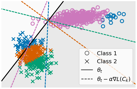
(a) GD step 0

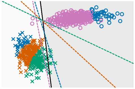
(b) GD step 1

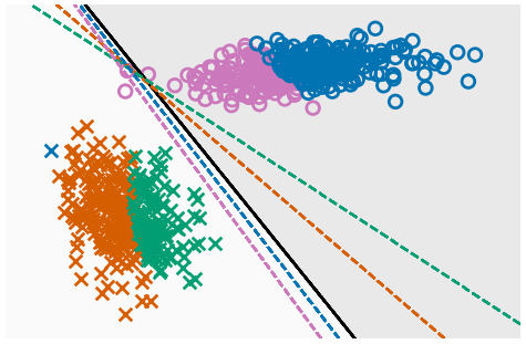
(c) GD step 2

Figure 1: Example of clusters found using Gradient Clustering. A linear classifier visualized during training with gradient descent on 2 linearly separable classes (o, x). Gradients are assigned to $4$ clusters (different colors) using Gradient Clustering (GC). Black line depicts current decision boundary. Colored dashed lines depict decision boundaries predicted from current boundary and each of the $4$ individual clusters. Here, blue points belong to both classes; they have similar gradients, but are far apart in input space. By exploiting the knowledge of GC we can get low variance average mini-batch gradients.

Contributions:

• Exploiting clustered distributions. We consider gradient distributions with distinct modes, i.e. the gradients can be clustered. We prove that the variance of average mini-batch gradient is minimized if the elements are sampled from a weighted clustering in gradient space (Section 3).

• Efficient clustering to minimize variance. We propose Gradient Clustering (GC) as a computationally efficient method for clustering in the gradient space (Section 3.2). Fig. 1 shows an example of clusters found by GC.

• Relation between gradient variance and optimization. We study the gradient variance on common deep learning benchmarks (MNIST, CIFAR-10, and ImageNet) as well as Random Features models recently studied in deep learning theory (Section 4). We observe that gradient variance increases during training, and smaller learning rates coincide with higher variance.

• An alternative statistic. We introduce normalized gradient variance as a statistic that better correlates with the speed of convergence compared to gradient variance (Section 4).

We emphasize that some of our contributions are primarily empirical yet unexpected. We encourage the reader to predict the behaviour of gradient variance before reaching our experiments section. We believe our results provide an opportunity for future theoretical and empirical work.

2 Related Work

Modeling gradient distribution. Despite various assumptions on the mini-batch gradient variance, there are limited studies of this statistic during the training of deep learning models. It is common to assume bounded variance in convergence analyses (Bottou et al., 2018). Works on variance reduction propose alternative estimates of the gradient mean with low variance (Le Roux et al., 2012; Johnson and Zhang, 2013) but they do not plot the variance which is the actual quantity they seek to reduce. Their ineffectiveness in deep learning has been observed but still requires explanation (Defazio and Bottou, 2019). There are a few works that present gradient variance plots (Mohamed et al., 2019; Wen et al., 2019) but they are usually for a single gradient coordinate and synthetic problems. The Central limit theorem is also used to argue that the distribution of the mini-batch gradient is a Gaussian (Zhu et al., 2019), which has been challenged only recently (Simsekli et al., 2019). There also exists a link between the Fisher (Amari, 1998), Neural Tangent Kernel (Jacot et al., 2018), and the gradient covariance matrix (Martens, 2014; Kunstner et al., 2019; Thomas et al., 2020). As such, any analysis of one (e.g. Karakida et al., 2019) could potentially be used to understand others.

The variance is rarely used for improving optimization. Le Roux et al. (2011) considered the difference between the covariance matrix of the gradients and the Fisher matrix and proposed incorporating the covariance matrix as a measure of model uncertainty in optimization. It has also been suggested that the division by the second moments of the gradient in Adam can be interpreted as variance adaptation (Kunstner et al., 2019). There are myriad papers on ad-hoc sampling and re-weighting methods for reducing dataset imbalance and increasing data diversity (Bengio and Senecal, 2008; Jiang et al., 2017; Vodrahalli et al., 2018; Jiang et al., 2019). Although we do not use Gradient Clustering for optimization, the formulation can be interpreted as a unifying approach that defines variance reduction as an objective.

Clustering gradients. Methods related to gradient clustering have been proposed in low-variance gradient estimation (Hofmann et al., 2015; Zhao and Zhang, 2014; Chen et al., 2019) supported by promising theory. However, these methods have either limited their experiments to linear models or treated a deep model as a linear one. Our proposed GC method performs efficient clustering in the gradient space with very few assumptions. GC is also related to works on model visualization where the entire training set is used to understand the behaviour of a model (Raghu et al., 2017).

3 Mini-batch Gradient with Stratified Sampling

An important factor affecting optimization trade-offs is the diversity of training data. SGD entails a sampling process, often uniformly sampling from the training set. However, as illustrated in the following example, uniform sampling is not always ideal. Suppose there are duplicate data points in a training set. We can save computation time by removing all but one of the duplicates. To get the same gradient mean in expectation, it is sufficient to rescale the gradient of the remaining sample in proportion to the number of duplicates. In this example, mini-batch SGD will be inefficient because duplicates increase the variance of the average gradient mean.

Suppose we are given i.i.d. training data, $\{{\bm{x}_{i}}\}_{i=1}^{N}$, and a partitioning of their gradients, ${\bm{g}_{i}}={\frac{\partial{}}{\partial\theta}}\ell({\bm{x}_{i}};{\bm{\theta}})$, into $K$ subsets, where ${N_{k}}$ is the size of the $k$-th set. We can estimate the gradient mean on the training set, $\bm{g}={\frac{\partial{}}{\partial\theta}}L({\bm{\theta}})$, by averaging $K$ gradients, one from each of $K$ subsets, uniformly sampled:

$${\bm{\hat{g}}}({\bm{a}}) =\frac{1}{N}{\sum_{k=1}^{K}}{N_{k}}\,{\bm{g}_{j,k}}\,,\quad j\sim{\mathbb{U}}[1,{N_{k}}]\,,$$ (1)

where $g_{.,k}=\{{\bm{g}_{i}}|{a_{i}}=k\}$ are the gradients from a subset $k$, ${\bm{g}_{j,k}}\in{\mathbb{R}}^{d}$ is the gradient of the $j$-th sample in the $k$-th subset, and ${\bm{a}}\in\{1,\ldots,K\}^{N}$ where ${a_{i}}$ is the index of the cluster to which $i$-th data point is assigned, so ${N_{k}}={\sum_{i=1}^{N}}{\mathbb{I}}({a_{i}}=k)$.  Each sample is treated as a representative of its subset and weighted by the size of that subset. In the limit of $K=N$, we recover the batch gradient mean used in GD and for $K=1$ we recover the single-sample stochastic gradient in SGD.

Proposition 3.1.

(Bias/Variance of Mini-batch Gradient with Stratified Sampling). For any partitioning of data, the estimator of the gradient mean using stratified sampling (Eq. 1) is unbiased (${\mathbb{E}}[{\bm{\hat{g}}}]=g$) and ${\mathbb{V}}[{\bm{\hat{g}}}]=N^{-2}{\sum_{k=1}^{K}}{N_{k}}^{2}{\mathbb{V}}[{\bm{g}_{j,k}}]$, where ${\mathbb{V}}[\cdot]$ is defined as the trace of the covariance matrix. (Proof in Section A.1)

Remark.

In a dataset with duplicate samples, the gradients of duplicates do not contribute to the variance if assigned to the same partition with no other data points.

3.1 Weighted Gradient Clustering

Suppose, for a given number of clusters, $K$, we want to find the optimal partitioning, i.e., one that minimizes the variance of the gradient mean estimator, ${\bm{\hat{g}}}$. For $d$-dimensional gradient vectors, minimizing the variance in 3.1, is equivalent to finding a weighted clustering of the gradients of data points,

$$\min_{\bm{a}}{\mathbb{V}}[{\bm{\hat{g}}}({a_{i}})] =\min_{\bm{a}}{\sum_{k=1}^{K}}{N_{k}}^{2}{\mathbb{V}}[{\bm{g}_{j,k}}]=\min_{\bm{C},{\bm{a}}}{\sum_{k=1}^{K}}{\sum_{i=1}^{N}}{N_{k}}\,\|{\bm{C}_{k}}-{\bm{g}_{i}}\|^{2}\,{\mathbb{I}}({a_{i}}=k)\,,$$ (2)

where a cluster center, ${\bm{C}_{k}}\in{\mathbb{R}}^{d}$, is the average of the gradients in the $k$-th cluster, and ${{\mathbb{V}}[{\bm{g}_{j,k}}]=\frac{1}{{N_{k}}}{\sum_{i=1}^{N}}\|{\bm{C}_{k}}-{\bm{g}_{i}}\|^{2}\,{\mathbb{I}}({a_{i}}=k)}$. If we did not have the factor ${N_{k}}$, this objective would be equivalent to the K-Means objective. The additional ${N_{k}}$ factors encourage larger clusters to have lower variance, with smaller clusters comprising scattered data points.

If we could store the gradients for the entire training set, the clustering could be performed iteratively as a form of block coordinate descent, alternating between the following Assignment and Update steps, i.e., computing the cluster assignments and then the cluster centers: $${\text{{$\mathcal{A}$} :}}\quad{a_{i}}=\operatorname*{arg\,min}_{k}{N_{k}}\,\|{\bm{C}_{k}}-{\bm{g}_{i}}\|^{2}$$ (3) $${\text{{$\mathcal{U}$} :}}\quad{\bm{C}_{k}}=\frac{1}{{N_{k}}}{\sum_{i=1}^{N}}{\bm{g}_{i}}\,{\mathbb{I}}({a_{i}}=k)$$ (4)

The $\mathcal{A}$ step is still too complex given the ${N_{k}}$ multiplier. As such, we first solve it for fixed cluster sizes then update ${N_{k}}$ before another $\mathcal{U}$ step. These updates are similar to Lloyd’s algorithm for K-Means, but with the ${N_{k}}$ multipliers, and to Expectation-Maximization for Gaussian Mixture Models, but here we use hard assignments. In contrast, the additional ${N_{k}}$ multiplier makes the objective more complex in that performing $\mathcal{AU}$ updates does not always guarantee a decrease in the clustering objective.

3.2 Efficient Gradient Clustering (GC)

Performing exact $\mathcal{AU}$ updates (Eqs. 3 and 4) is computationally expensive as they require the gradient of every data point. Deep learning libraries usually provide efficient methods that compute average mini-batch gradients without ever computing full individual gradients. We introduce Gradient Clustering (GC) for performing efficient $\mathcal{AU}$ updates by breaking them into per-layer operations and introducing a low-rank approximation to cluster centers.

Algorithm 1 $\mathcal{A}$ step using Eq. 5

  for $i=1$ to $N$ do

     for $k=1$ to $K$ do

        for $l=1$ to $L$ do

           $D_{kl}=\|\bm{C}_{kl}-\bm{g}_{il}\|^{2}$

     $\bm{S}=\sum_{l}D_{\cdot l}$

     ${a_{i}}=\operatorname*{arg\,min}_{k}{N_{k}}\bm{S}$

Algorithm 2 ${N_{k}}$ update

  ${N_{k}}=0,\quad\forall k={1,\cdots,K}$

  for $i=1$ to $N$ do

     $N_{{a_{i}}}\mathrel{+}=1$

Algorithm 3 $\mathcal{U}$ step using Eq. 6

  $\bm{C}_{k}=0,\quad\forall k={1,\cdots,K}$

  for $i=1$ to $N$ do

     for $l=1$ to $L$ do

        $\bm{C}_{{a_{i}},l}\mathrel{+}=\bm{g}_{il}/N_{{a_{i}}}$

Figure 2: Steps in Gradient Clustering

For any feed-forward network, we can decompose terms in $\mathcal{AU}$ updates into independent per-layer operations as shown in Fig. 2. The main operations are computing $\|\bm{C}_{kl}-\bm{g}_{il}\|^{2}$ and cluster updates $\bm{C}_{{a_{i}},l}\mathrel{+}=\bm{g}_{il}/N_{{a_{i}}}$ per layer $l$; henceforth, we drop the layer index for simplicity.

For a single fully-connected layer, we denote the layer weights by ${\bm{\theta}}\in{\mathbb{R}}^{{I}\times{O}}$, where ${I}$ and ${O}$ denote the input and output dimensions for the layer. We denote the gradient with respect to ${\bm{\theta}}$ for the training set by $\bm{g}={\bm{A}}{\bm{D}}^{\top}$, where ${\bm{A}}\in{\mathbb{R}}^{{I}\times N}$ comprises the input activations to the layer, and ${\bm{D}}\in{\mathbb{R}}^{{O}\times N}$ represents the gradients with respect to the layer outputs. The coordinates of cluster centers corresponding to this layer are denoted by $C\in{\mathbb{R}}^{K\times{I}\times{O}}$. We index the clusters using $k$ and the data by $i$. The $k$-th cluster center is approximated as ${{\bm{C}_{k}}={\bm{c}_{k}}{\bm{d}_{k}}^{\top}}$, using vectors ${{\bm{c}_{k}}\in{\mathbb{R}}^{I}}$ and ${{\bm{d}_{k}}\in{\mathbb{R}}^{O}}$.

In the $\mathcal{A}$ step we need to compute ${\|{\bm{C}_{k}}-{\bm{g}_{i}}\|_{F}^{2}}$ as part of the assignment cost, where $\|\cdot\|_{F}$ is the Frobenius-norm. We expand this term into three inner-products, and compute them separately. In particular, the term ${{\mathcal{\text{vec}}{{\{{\bm{C}_{k}}\}}}}}\odot{{\mathcal{\text{vec}}{{\{{\bm{g}_{i}}\}}}}}$ can be written as,

$${{\mathcal{\text{vec}}{{\{{\bm{C}_{k}}\}}}}}\odot{{\mathcal{\text{vec}}{{\{{\bm{A}_{i}}{\bm{D}_{i}}^{\top}\}}}}}=({\bm{A}_{i}}\odot{\bm{c}_{k}})({\bm{D}_{i}}\odot{\bm{d}_{k}})\,,$$ (5)

where $\odot$ denotes inner product, and the RHS is the product of two scalars. Similarly, we compute the other two terms in the expansion of the assignment cost, i.e. ${{\mathcal{\text{vec}}{{\{{\bm{C}_{k}}\}}}}}\odot{{\mathcal{\text{vec}}{{\{{\bm{C}_{k}}\}}}}}$ and ${{\mathcal{\text{vec}}{{\{{\bm{g}_{i}}\}}}}}\odot{{\mathcal{\text{vec}}{{\{{\bm{g}_{i}}\}}}}}$ (Goodfellow (2015) proposed a similar idea to compute the gradient norm).

The $\mathcal{U}$ step in Eq. 4 is written as, ${\bm{c}_{k}}{\bm{d}_{k}}^{\top}={N_{k}}^{-1}{\sum_{i=1}^{N}}{\bm{A}_{i}}{\bm{D}_{i}}^{\top}{\mathbb{I}}({a_{i}}=k)$. This equation might have no exact solution for ${\bm{c}_{k}}$ and ${\bm{d}_{k}}$ because the sum of rank-$1$ matrices is not necessarily rank-$1$. One approximation is the min-Frobenius-norm solution to ${\bm{c}_{k}},{\bm{d}_{k}}$ using truncated SVD, where we use left and right singular-vectors corresponding to the largest singular-value of the RHS. However, the following updates are exact if activations and gradients of the outputs are uncorrelated, i.e. ${\mathbb{E}}_{i}[{\bm{A}_{i}}{\bm{D}_{i}}]={\mathbb{E}}_{i}[{\bm{A}_{i}}]E_{i}[{\bm{D}_{i}}]$ (similar to assumptions in K-FAC (Martens and Grosse, 2015)),

$${\bm{c}_{k}}=\frac{1}{{N_{k}}}{\sum_{i=1}^{N}}{\bm{A}_{i}}{\mathbb{I}}({a_{i}}=k)\qquad\qquad{\bm{d}_{k}}=\frac{1}{{N_{k}}}{\sum_{i=1}^{N}}{\bm{D}_{i}}{\mathbb{I}}({a_{i}}=k)\,.$$ (6)

In Section B.1, we describe similar update rules for convolutional layers and in Section B.2, we provide complexity analysis of GC. We can make the cost of GC negligible by making sparse incremental updates to cluster centers using mini-batch updates. The assignment step can also be made more efficient by processing only a portion of data as is common for training on large datasets. The rank-$1$ approximation can be extended to higher rank approximations with multiple independent cluster centers though with challenges in the implementation.

4 Experiments

In this section, we evaluate the accuracy of estimators of the gradient mean. This is a surrogate task for evaluating the performance of a model of the gradient distribution. We compare our proposed GC estimator to average mini-batch Stochastic Gradient (SG-B), and SG-B with double the mini-batch size (SG-2B). SG-2B is an important baseline for two reasons. First, it is a competitive baseline that always reduces the variance by a factor of $2$ and requires at most twice the memory size and twice the run-time per mini-batch (Shallue et al., 2018). Second, the extra overhead of GC is approximately the same as keeping an extra mini-batch in the memory when the number of clusters is equal to the mini-batch size. We also include Stochastic Variance Reduced Gradient (SVRG) (Johnson and Zhang, 2013) as a method with the sole objective of estimating gradient mean with low variance.

We compare methods on a single trajectory of mini-batch SGD to decouple the optimization from gradient estimation. That is, we do not train with any of the estimators (hence no ‘D’ in SG-B and SG-2B). This allows us to continue analyzing a method even after it fails in reducing the variance. For training results using SG-B, SG-2B and, SVRG, we refer the reader to Shallue et al. (2018); Defazio and Bottou (2019). For training with GC, it suffices to say that behaviours observed in this section are directly related to the performance of GC used for optimization.

As all estimators in this work are unbiased, the estimator with lowest variance is better estimating the gradient mean. We define Average Variance (variance in short) as the average over all coordinates of the variance of the gradient mean estimate for a fixed model snapshot. Average variance is the normalized trace of the covariance matrix and of particular interest in random matrix theory (Tao, 2012). We also measure Normalized Variance, defined as ${\mathbb{V}}[g]/E[g^{2}]$ where the variance of a $1$-dimensional random variable is divided by its second non-central moment. In signal processing, the inverse of this quantity is the signal to noise ratio (SNR). If SNR is less than one (normalized gradient larger than one), the power of the noise is greater than the signal. Additional details of the experimental setup can be found in Appendix C.

4.1 MNIST: Low Variance, CIFAR-10: Noisy Estimates, ImageNet: No Structure

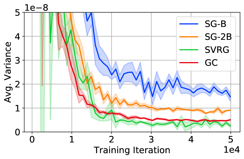
(a) MLP on MNIST

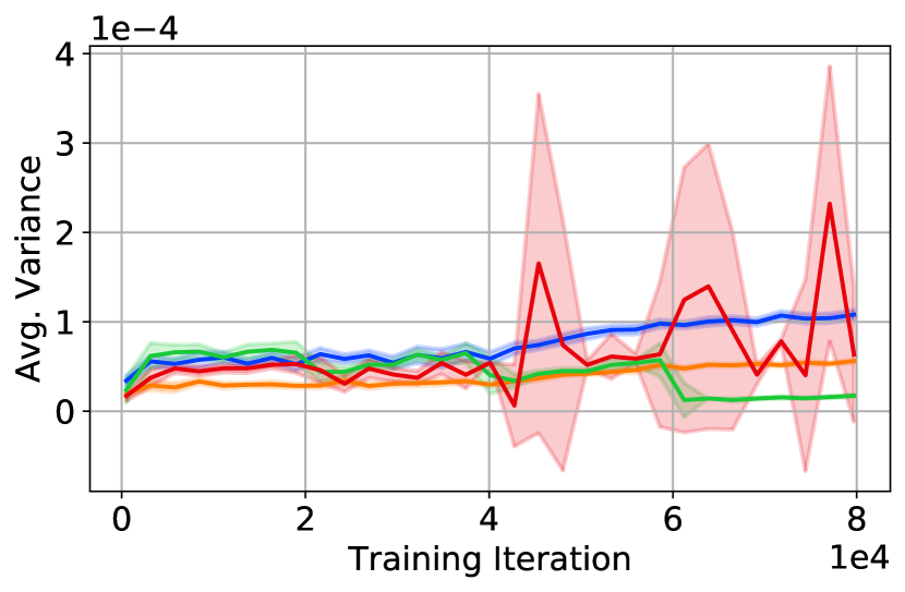
(b) ResNet8 on CIFAR-10

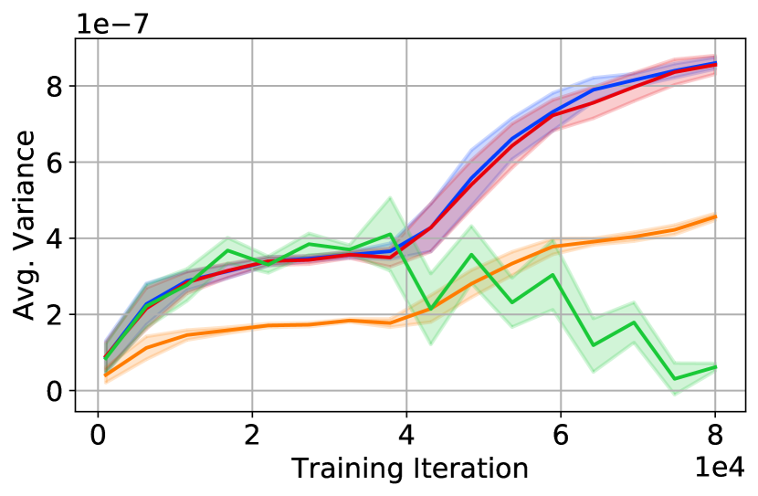
(c) ResNet18 on ImageNet

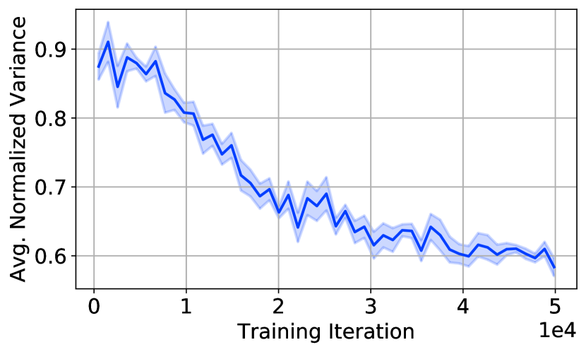
(d) MLP on MNIST

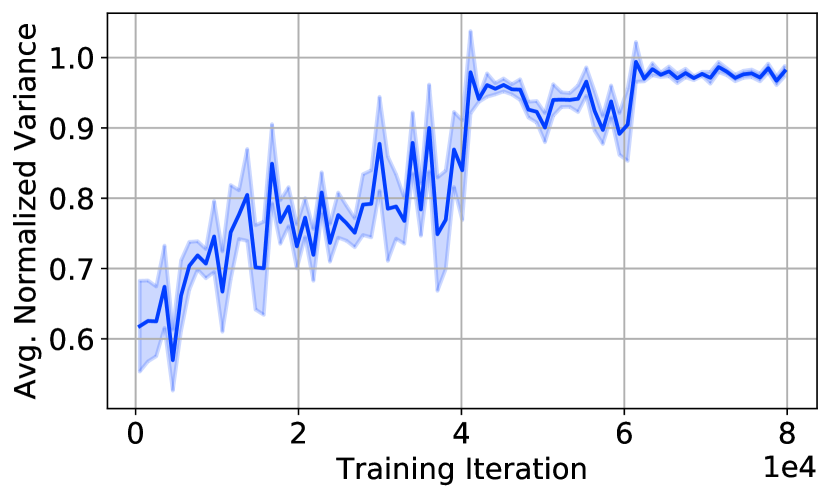
(e) ResNet8 on CIFAR-10

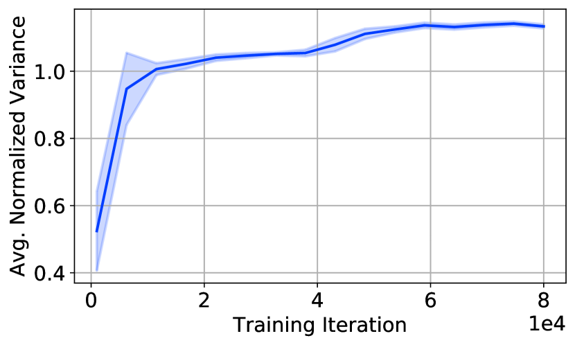
(f) ResNet18 on ImageNet

Figure 3: Image classification models. Variance (top) and normalized variance plots (bottom). We observe: normalized variance correlates with optimization difficulty, variance is decreasing on MNIST but increasing on CIFAR-10 and ImageNet, and variance fluctuates with GC on CIFAR-10.

In this section, we study the evolution of gradient variance during training of an MLP on MNIST (LeCun et al., 1998), ResNet8 (He et al., 2016) on CIFAR-10 (Krizhevsky et al., 2009), and ResNet18 on ImageNet (Deng et al., 2009). Curves shown are from a single run and statistics are smoothed out over a rolling window. The standard deviation within the window is shown as a shaded area.

Normalized variance correlates with the time required to improve accuracy. In Figs. 3(a), 3(b) and 3(c), the variance of SG-2B is always half the variance of SG-B. A drawback of the variance is that it is not comparable across different problems. For example, on CIFAR-10 the variance of all methods reaches $10^{-4}$ while on ImageNet where usually $10\times$ more iterations are needed, the variance is below $10^{-6}$. In Figs. 3(d), 3(e) and 3(f), normalized variance better correlates with the convergence speed. Normalized variance on both MNIST and CIFAR-10 is always below $1$ while on ImageNet it quickly goes above $1$ (noise stronger than gradient). Notice that the denominator in the normalized variance is shared between all methods on the same trajectory of mini-batch SGD. As such, the normalized variance retains the relation of curves and is a scaled version of variance where the scaling varies during training as the norm of the gradient changes. For clarity, we only show the curve for SG-B.

How does the difficulty of optimization change during training? The variance on MNIST for all methods is constantly decreasing (Fig. 3(a)), i.e. the strength of noise decreases as we get closer to a local optima. These plots suggest that training an MLP on MNIST satisfies the Strong Growth Condition (SGC) (Schmidt and Le Roux, 2013) as the variance is numerically zero (below $10^{-8}$). Normalized variance (Fig. 3(d)) decreases over time and is well below $1$ (gradient mean has larger magnitude than the variance). SVRG performs particularly well by the end of the training because the training loss has converged to near zero (cross-entropy less than $0.005$). Promising published results with SVRG are usually on datasets similar to MNIST where the loss reaches relatively small values. In contrast, on both CIFAR-10 (Figs. 3(b) and 3(e)) and ImageNet (Figs. 3(c) and 3(f)), the variance and normalized variance of all methods increase during training and especially after the learning rate drops. This means gradient variance depends on the distance to local optima. We hypothesize that the gradient of each training point becomes more unique as training progresses.

Variance can widely change during training but it happens only on a particularly noisy data. On CIFAR-10, the variance of GC suddenly goes up but comes back down before any updates to the cluster centers (Fig. 3(b)) while the variance of SVRG monotonically increases between updates. To explain these behaviours, notice that immediately after cluster updates, GC and SVRG should always have at most the same average variance as SG-B. We observed this behaviour consistently across different architectures such as other variations of ResNet and VGG on CIFAR-10. Fig. 7 shows the effect of adding noise on CIFAR-10. Label smoothing (Szegedy et al., 2016) reduces fluctuations but not completely. On the other hand, label corruption, where we randomly change the labels for $10\%$ of the training data eliminates the fluctuations. We hypothesize that the model is oscillating between different states with significantly different gradient distributions. The experiments with corrupt labels suggest that mislabeled data might be the cause of fluctuations such that having more randomness in the labels forces the model to ignore originally mislabeled data.

Is the gradient distribution clustered in any dataset? The variance of GC on MNIST (Fig. 3(a)) is consistently lower than SG-2B which means it is exploiting clustering in the gradient space. On CIFAR-10 (Fig. 3(b)) the variance of GC is lower than SG-B but not lower than SG-2B except when fluctuating. The improved variance is more noticeable when training with corrupt labels. On ImageNet (Figs. 3(c) and 3(f)), the variance of GC is overlapping with SG-B. An example of a gradient distribution where GC is overlapping with SG-B is a uniform distribution. Gradient distribution can still be structured. For example, there could be clusters in subspaces of the gradient space.

4.2 Random Features Models: How Does Overparametrization Affect the Variance?

The Random Features (RF) model (Rahimi and Recht, 2007) provides an effective way to explore the behaviour of optimization methods across a family of learning problems. The RF model facilitates the discovery of optimization behaviours including the double-descent shape of the risk curve (Hastie et al., 2019; Mei and Montanari, 2019). We train a student RF model with hidden dimensions $h_{s}$ on a fixed training set, $(\bm{x}_{i},\bm{y}_{i})\in{\mathbb{R}}^{I}\times\{\pm 1\}$, $i=1,\ldots,N$, sampled from a model, ${\bm{x}_{i}\sim{\mathcal{N}}(0,{\mathbb{I}})}$, ${\bm{y}_{i}=\operatorname*{sign}(\sigma(\bm{x}_{i}^{\top}\bm{\hat{\theta_{1}}})^{\top}\bm{\hat{\theta_{2}}}+b)}$ where $\sigma$ is the ReLU activation function, and the teacher hidden features $\bm{\hat{\theta_{1}}}\in{\mathbb{R}}^{I\times h_{t}}$, and second layer weights and bias, $\bm{\hat{\theta_{2}}}\in{\mathbb{R}}^{h_{t}\times 1},b\in{\mathbb{R}}$, are sampled from the standard normal distribution. Each $I$ dimensional random feature of the teacher is scaled to $\ell_{2}$ norm 1. We train a student RF model with random features $\bm{\theta_{1}}\in{\mathbb{R}}^{I\times h_{s}}$ and second layer weights $\bm{\theta_{2}}\in{\mathbb{R}}^{h_{s}\times 1}$ by minimizing the cross-entropy loss. In Fig. 4, we train hundreds of Random Features models and plot the average variance and normalized variance of gradient estimators. We show both maximum and mean of the statistics during training. The maximum better captures fluctuations of a gradient estimator and allows us to link our observations of variance to generalization using standard convergence bounds that rely on bounded noise (Bottou et al., 2018).

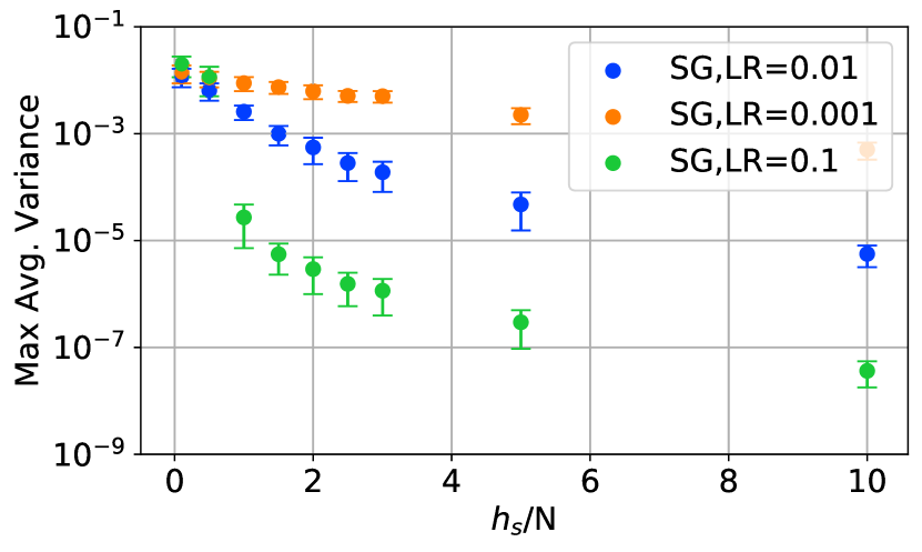
(a) $3$ SGD trajectories

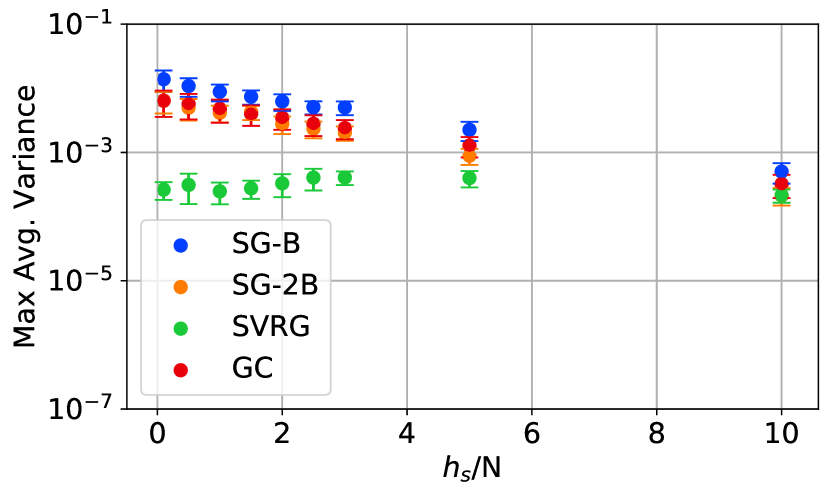
(b) Trajectory of LR=$0.001$

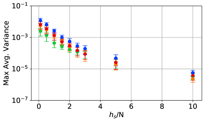
(c) Trajectory of LR=$0.01$

Figure 4: Random Features models. Variance (log-scale) versus the over-parametrization coefficient (student’s hidden divided by the training set size). We observe: teacher’s hidden is not influential, variance is low in overparametrized regime, and with larger learning rates. We aggregate results from hyperparameters not shown.

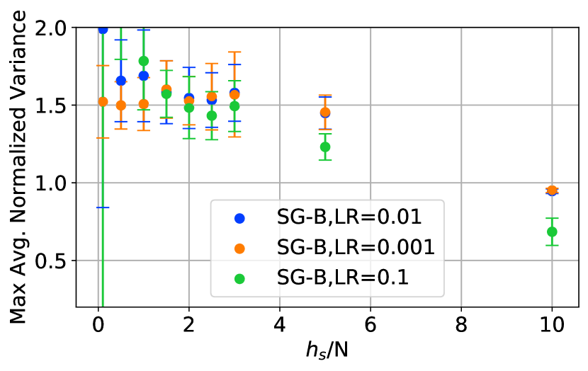
(a) SGD max norm. var.

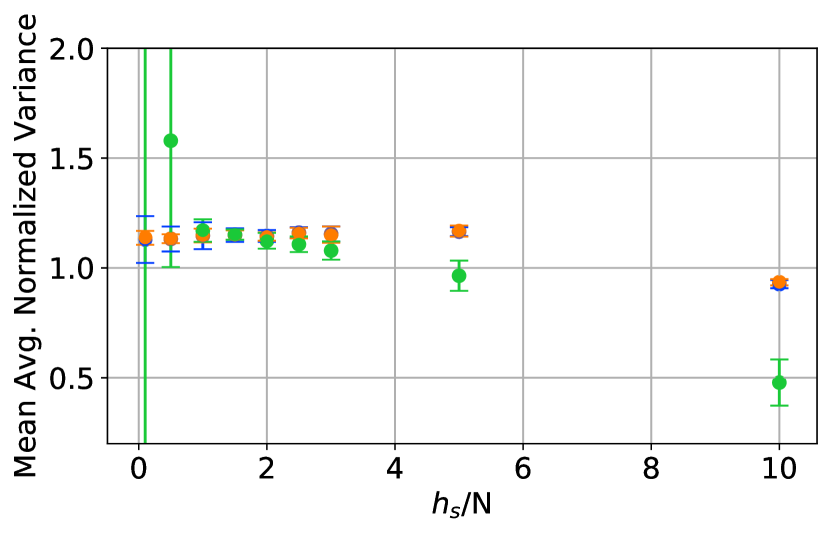
(b) SGD mean norm. var.

Figure 5: Normalized variance on overparam. RF is less than $1$.

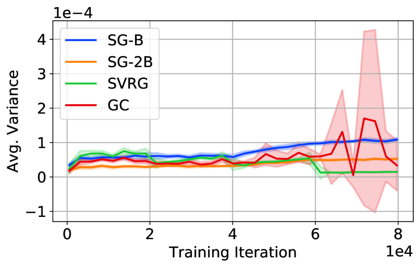
(c) Label smoothing

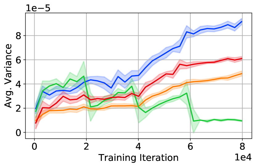
(d) Corrupt labels

Figure 6: CIFAR-10 Fluctuations disappear with corrupt labels.

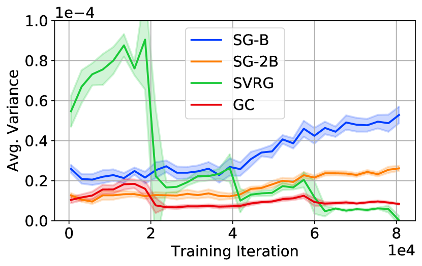
(a) CIFAR-10

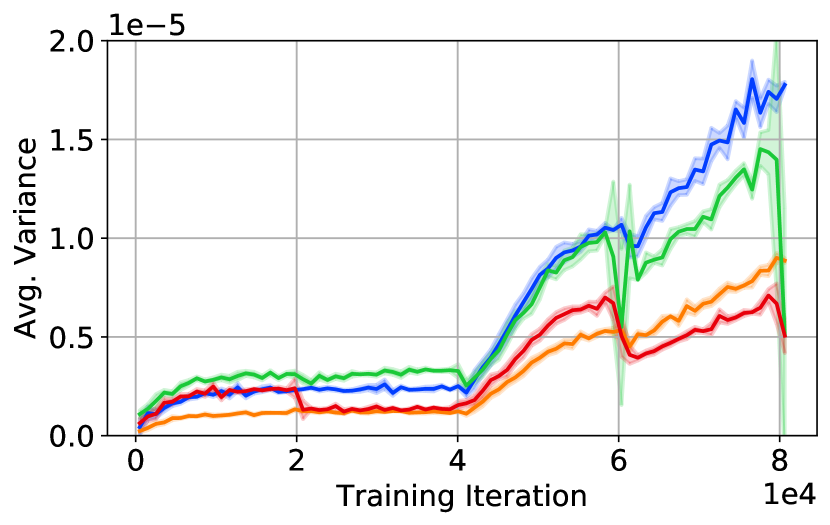
(b) CIFAR-100

Figure 7: Image classification with duplicates exploited by GC.

Do models with small generalization gap converge faster? Based on small error bars, the only hyperparameters that affect the variance are learning rate and the ratio of the size of the student hidden layer over the training set size. In contrast, in analysis of risk and the double descent phenomena, we usually observe a dependence on ratio of the student hidden layer size to the teacher hidden layer size (Mei and Montanari, 2019). This suggests that models that generalize better are not necessarily ones that train faster.

Does “diminishing returns” happen because of overparametrization? Figs. 4(b) and 4(c) show that with the same learning rate, all methods achieve similar variance in the overparametrized regime. Note that due to the normalization of random features, the gradients in each coordinate are expected to decrease as overparametrization increases. We conjecture that the diminishing returns in increasing the mini-batch size should also be observed in overparametrized random features models similar to linear and deeper models (Zhang et al., 2019; Shallue et al., 2018).

Why does the loss usually drop immediately after a learning rate drop? Fig. 4(a) shows that the variance is smaller for trajectories with larger learning rates and that the gap grows as overparametrization grows. This is a direct consequence of the dependence of the noise in the gradient on current parameters. In Section 4.1 we observe the opposite of this behaviour in deep models. In contrast, Fig. 7 shows that for overparametrization less than $5$, all trajectories have similar normalized variance that is larger than one (noise is more powerful than the gradient). As such, we hypothesize that the reduction in variance is not the sole reason for the immediate decrease in the loss after a learning rate drop (e.g. He et al., 2016).

How does SGD avoid local minima? In Fig. 5(a), the error bars in the maximum normalized variance are long for overparametrization coefficient less than $5$. The reason is in some iterations the second moment of the gradient for some coordinates gets close to zero but the noise due to mini-batching is still non-zero. Often in the next iteration, the gradient becomes large again. This is an example where SGD avoids local minima due to noise.

Why does SVRG fail in deep learning? Figs. 4(b) and 4(c) show that the gain of SVRG vanishes in the over-parametrized regime ($10$) where all methods have relatively low variance (below $10^{-5}$). We hypothesize that the cause is the generally lower variance of the noise in the overparametrized regime rather than the staleness of the control-variate.

4.3 Duplicates: Back to the Motivation for Gradient Clustering

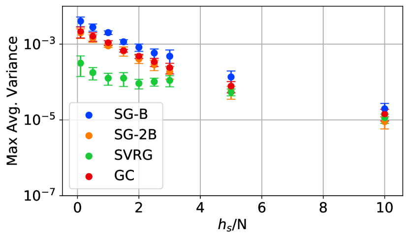
(a) $10\%$ duplicates

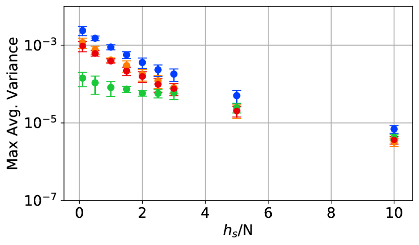
(b) $50\%$ duplicates

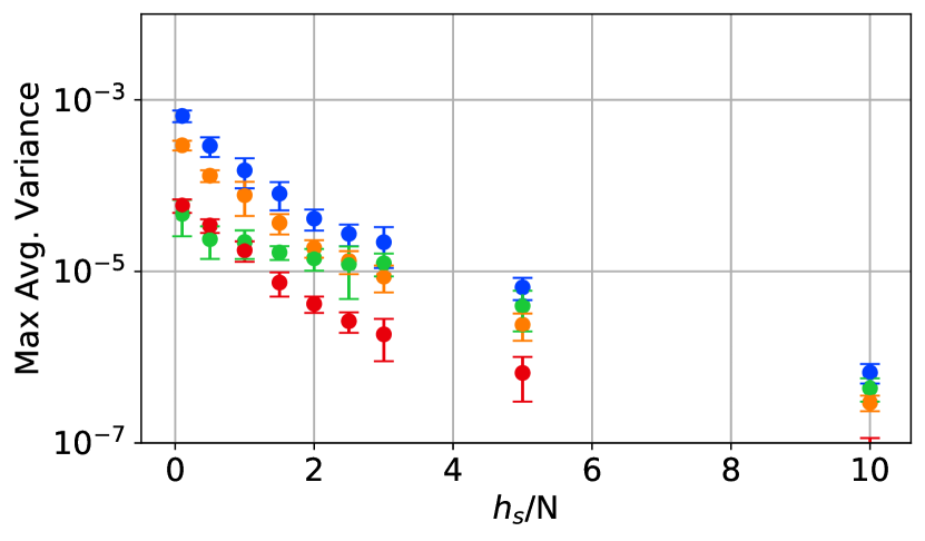
(c) $90\%$ duplicates

Figure 8: Training RF Models with Duplicates. GC identifies and exploits duplicates. Plots are similar to Fig. 4. Learning rate in all three is $0.01$. In each training, there are $5$ data points that are repeated equally to make up $10\%$ (left), $50\%$ (middle), and $90\%$ (right) of the training set.

In Fig. 8, we trained random features models with additional duplicated data points. We observe that as the ratio of duplicates to non-duplicates increases, the gap between the variance of GC and other methods improve. Without duplicate data, GC is always between SG-B and SG-2B. It is almost never worse than SG-B and never better than SG-2B. GC is as good as SG-2B at mild overparametrization ($1-4$). We need a degree of overparametrization for GC to reduce the variance but too much overparametrization leaves no room for improvement. When duplicates exist, GC performs well with a gap that does not decrease by overparametrization.

Similarly, experiments on CIFAR-10 and CIFAR-100 (Fig. 7) show that GC significantly reduces the variance when duplicate data points exist. Note that because of common data augmentations, duplicate data points are not exactly duplicate in the input space and there is no guarantee that their gradients would be similar.

5 Conclusion

In this work we introduced tools for understanding the optimization behaviour and explaining previously perplexing observations in deep learning. We expect our contributions to not only guide improvements to optimization speed and generalization but also the design of interpretable models. We have provided evidence that structured gradient distributions such as clustered gradients exist and that statistics of gradients can provide insight into the optimization performance. However, exploiting this knowledge to improve optimization has proven to be challenging.

Appendix A Additional Details of Gradient Clustering (Section 3)

A.1 Proof of 3.1

The gradient estimator, ${\bm{\hat{g}}}$, is unbiased for any partitioning of data, i.e. equal to the average gradient of the training set,

$${\mathbb{E}}[{\bm{\hat{g}}}] =\frac{1}{N}{\sum_{k=1}^{K}}{N_{k}}{\mathbb{E}}[{\bm{g}_{j,k}}]=\frac{1}{N}{\sum_{k=1}^{K}}{N_{k}}\left(\frac{1}{{N_{k}}}{\sum_{j=1}^{N_{k}}}{\bm{g}_{j,k}}\right)=\underbrace{\frac{1}{N}{\sum_{k=1}^{K}}{\sum_{j=1}^{N_{k}}}{\bm{g}_{j,k}}}_{(*)}=\frac{1}{N}{\sum_{i=1}^{N}}{\bm{g}_{i}}=\bm{g}~{},$$

where we use the fact that the expectation of a random sample drawn uniformly from a subset is equal to the expectation of the average of samples from that subset. Also note that the gradient of every training example appears once in $(*)$.

Although partitioning does not affect the bias of ${\bm{\hat{g}}}$, it does affect the variance,

$${\mathbb{V}}[{\bm{\hat{g}}}] =\frac{1}{N^{2}}\left({\sum_{i=1}^{N}}{N_{k}}^{2}{\mathbb{V}}[{\bm{g}_{j,k}}]+2{\sum_{k=1}^{K}}\sum_{\hat{k}=1}^{N_{\hat{k}}}{N_{k}}N_{\hat{k}}{\mathbb{C}}[{\bm{g}_{j,k}},\bm{g}_{\hat{j},\hat{k}}]\right)=\frac{1}{N^{2}}{\sum_{k=1}^{K}}{N_{k}}^{2}{\mathbb{V}}[{\bm{g}_{j,k}}]$$ (7)

where the variance is defined as the trace of the covariance matrix. Since we assume the training set is sampled i.i.d., the covariance between gradients of any two samples is zero. In a dataset with duplicate samples, the gradients of duplicates will be clustered into one cluster with zero variance if mingled with no other data points.

Appendix B Additional Details of Efficient GC (Section 3.2)

B.1 Convolutional Layers

In neural networks, the convolution operation is performed as an inner product between a set of weights ${\bm{\theta}}\in{\mathbb{R}}^{h\times w\times\hat{{I}}\times{O}}$, namely kernels, by patches of size $h\times w$ in the input. Assuming that we have preprocessed the input by extracting patches, the gradient w.r.t. ${\bm{\theta}}$ is ${\bm{g}_{i}}={\sum_{t}\bm{g}_{b,t}}$, $\bm{g}_{b,t}\in{\mathbb{R}}^{{I}\times{O}}$ is the gradient at the spatial location $t\in T$ and ${I}=h\times w\times\hat{{I}}$ is the flattened dimension of a patch. The gradient at spatial location $t$ is computed as $\bm{g}_{b,t}={\bm{A}}_{b,t}{\bm{D}}_{b,t}^{\top}$.

Like the fully-connected case, we use a rank-$1$ approximation to the cluster centers in a convolution layer, defining ${\bm{C}_{k}}={\bm{c}_{k}}{\bm{d}_{k}}^{\top}$. As such, $\mathcal{AU}$ steps are performed efficiently. For the $\mathcal{A}$ step we rewrite ${{{\mathcal{\text{vec}}{{\{{\bm{C}_{k}}\}}}}}\odot{{\mathcal{\text{vec}}{{\{{\bm{g}_{i}}\}}}}}}$,

$${{\mathcal{\text{vec}}{{\{{\bm{C}_{k}}\}}}}}\odot{{\mathcal{\text{vec}}{{\{\sum_{t}{\bm{A}}_{b,t}{\bm{D}}_{b,t}^{\top}\}}}}} =\sum_{u,v}(\bm{c}_{ku}~{}\bm{d}_{kv}~{}~{}(\sum_{t}{\bm{A}}_{btu}~{}{\bm{D}}_{btv}))$$ (8)

$$=\sum_{t}(\sum_{u}\bm{c}_{ku}~{}{\bm{A}}_{btu})(\sum_{v}\bm{d}_{kv}~{}{\bm{D}}_{btv}),$$ (9)

where the input dimension is indexed by $u$ and the output dimension is indexed by $v$. Eqs. 8 and 9 provide two ways of computing the inner-product, where we first compute the inner sums, then the outer sum. The efficiency of each formulation depends on the size of the kernel and layer’s input and output dimensions.

B.2 Complexity Analysis

Operation	FC Complexity	Conv Complexity
$\bm{C}\odot\bm{g}$	$KB({I}+{O})$	Eq. 8: $B(T+K){I}{O}$ Eq. 9: $BTK({I}+{O})$
$\bm{C}\odot\bm{C}$	$K({I}+{O})$	$K({I}+{O})$
$\bm{g}\odot\bm{g}$	$B({I}+{O})$	Eq. 8: $BT{I}{O},$ Eq. 9: $BT^{2}({I}+{O})$
Back-prop	$B{I}{O}$	$BT{I}{O}$
$\mathcal{A}$ step	$KB({I}+{O})$	See Sec. B.2
$\mathcal{U}$ step	$B({I}+{O})$	$B({I}+{O})$

Table 1: Complexity of GC compared to the cost of back-prop.

GC, described in Fig. 2, performs two sets of operations, namely, the cluster center updates ($\mathcal{U}$ step), and the assignment update of data to clusters ($\mathcal{A}$ step). $\mathcal{A}$ steps instantly affect the optimization by changing the sampling process. As such, we perform an $\mathcal{A}$ step every few epochs and change the sampling right after. In contrast, the $\mathcal{U}$ step can be done in parallel and more frequently than the $\mathcal{A}$ step, or online using mini-batch updates. The cost of both steps is amortized over optimization steps.

Table 1 summarizes the run-time complexity of GC compared to the cost of single SGD step. The $\mathcal{U}$ step is always cheaper than a single back-prop step. The $\mathcal{A}$ step is cheaper for fully-connected layers if ${K<\min({I},{O})}$.

For convolutional layers, we have two ways to compute the terms in the $\mathcal{A}$ step (Eqs. 8 and 9). For ${\bm{C}\odot\bm{g}}$, if ${\min(T,K)}<{K<\min({I},{O})}$, Eq. 9 is more efficient. For ${\bm{g}\odot\bm{g}}$, Eq. 9 is more efficient if $T<\min(I,O)$. If $K<T$, both methods have lower complexity than a single back-prop step. If we did not have the ${N_{k}}$ multiplier in the $\mathcal{A}$ step, we could ignore the computation of the norm of the gradients, and hence further reduce the cost.

In common neural network architectures, the condition $K<T$ is easily satisfied as $T$ in all layers is almost always more than $10$ and usually greater than $100$, while $10$-$100$ clusters provides significant variance reduction. As such, the total overhead cost with an efficient implementation is at most $2\times$ the cost of a normal back-prop step. We can further reduce this cost by performing GC on a subset of the layers, e.g. one might exclude the lowest convolutional layers.

The total memory overhead is equivalent to increasing the mini-batch size by $K$ samples as we only need to store rank-$1$ approximations to the cluster centers.

Appendix C Additional Details for Experiments (Section 4)

The mini-batch size in GC and SVRG and the number of clusters in GC are the same as the mini-batch size in SG-B and the same as the mini-batch size used for training using SGD. To measure the gradient variance, we take snapshots of the model during training, sample tens of mini-batches from the training set (in case of GC, with stratified sampling), and measure the average variance of the gradients.

We measure the performance metrics (e.g. loss, accuracy and variance) as functions of the number of training iterations rather than wall-clock time. In other words, we do not consider computational overhead of different methods. In practice, such analysis is valid as long as the additional operations could be parallelized with negligible cost.

C.1 Experimental Details for Image Classification Models (Section 4.1)

On MNIST, our MLP model consists of there fully connected layers: layer1: $28*28\times 1024$, layer2: $1024\times 1024$, layer3: $1024,10$. We use ReLU activations and no dropout in this MLP. We train all methods with learning rate $0.02$, weight decay $5\times 10^{-4}$, and momentum $0.5$. On CIFAR-10, we train ResNet8 with no batch normalization layer and learning rate $0.01$, weight decay $5\times 10^{-4}$, and momentum $0.9$ for $80000$ iterations. We decay the learning rate at $40000$ and $60000$ iterations by a factor of $0.1$. On CIFAR-100, we train ResNet32 starting with learning rate $0.1$. Other hyper-parameters are the same as in CIFAR-10. On ImageNet, we train ResNet18 starting with learning rate $0.1$, weight decay $1\times 10^{-4}$, and momentum $0.9$. We use a similar learning rate schedule to CIFAR-10.

Dataset	Model	$B$	T	Log T	Estim T	U	GC T
MNIST	MLP	$128$	$50000$	$500$	$50$	$2000$	$10$
CIFAR-10	ResNet8	$128$	$80000$	$500$	$50$	$20000$	$3$
CIFAR-100	ResNet32	$128$	$80000$	$500$	$50$	$20000$	$3$
ImageNet	ResNet18	$128$	$80000$	$1000$	$10$	$10000$	$3$

Table 2: Hyperparameters.

In Table 2 we list the following hyperparameters: the interval of measuring gradient variance and normalized variance (Log T), number of gradient estimates used on measuring variance (Estim T), the interval of updating the control variate in SVRG and the clustering in GC (U), and the number of GC update iterations (GC T).

In plots for random features models, each point is generated by keeping $h_{s}$ fixed at $1000$ and varying $N$ in the range $[0.1,10]$. We average over $3$ random seeds, $2$ teacher hidden dimensions and $2$ input dimensions (both $\times 0.1$ and $\times 10$ student hidden). We use mini-batch size $10$ for SG-B, SVRG, and GC.

A rough estimate of the overparametrization coefficient (discussed in Section 4.2) for deep models is to divide the total number of parameters by the number of training data. On MNIST the coefficient is approximately $37$ for CNN and $31$ for MLP. On CIFAR-10 it is approximately $3$ for ResNet8 and $9$ for ResNet32. Common data augmentations increase the effective training set size by $10\times$. On the other hand, the depth potentially increases the capacity of models exponentially (cite the paper that theoretically says how many data points a model can memorize). As such, it is difficult to directly relate these numbers to the behaviours observed in RF models.

C.2 Experimental Details for Random Features Models (Section 4.2)

The number of training iterations is chosen such that the training loss has flattened. The maximum is taken over the last $70\%$ of iterations (the variance is usually high for all methods in the first $30\%$). Mean variance plots for random features models are similar to max variance plots presented in Section 4.2.

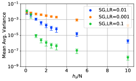
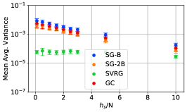
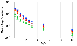
Figure 9: Mean variance plots for Fig. 4

We aggregate results from multiple experiments with the following range of hyperparameters. Each point is generated by keeping $h_{s}$ fixed at $1000$ and varying $N$ in the range $[0.1,10]$. We average over $3$ random seeds, $2$ teacher hidden dimensions and $2$ input dimensions (both $\times 0.1$ and $\times 10$ student hidden).

References

- Amari (1998) Shun-Ichi Amari. Natural gradient works efficiently in learning. Neural computation, 10(2):251–276, 1998.
- Bengio and Senecal (2008) Yoshua Bengio and Jean-Sébastien Senecal. Adaptive importance sampling to accelerate training of a neural probabilistic language model. IEEE Trans. Neural Networks, 19(4):713–722, 2008.
- Bottou et al. (2018) Léon Bottou, Frank E. Curtis, and Jorge Nocedal. Optimization methods for large-scale machine learning. SIAM Review, 60(2):223–311, 2018.
- Chen et al. (2019) Beidi Chen, Yingchen Xu, and Anshumali Shrivastava. Fast and accurate stochastic gradient estimation. In Neural Information Processing Systems (NeurIPS), pages 12339–12349, 2019.
- Defazio and Bottou (2019) Aaron Defazio and Léon Bottou. On the ineffectiveness of variance reduced optimization for deep learning. In Neural Information Processing Systems (NeurIPS), pages 1753–1763, 2019.
- Deng et al. (2009) Jia Deng, Wei Dong, Richard Socher, Li-Jia Li, Kai Li, and Fei-Fei Li. Imagenet: A large-scale hierarchical image database. In Conference on Computer Vision and Pattern Recognition (CVPR), pages 248–255. IEEE Computer Society, 2009.
- Golmant et al. (2018) Noah Golmant, Nikita Vemuri, Zhewei Yao, Vladimir Feinberg, Amir Gholami, Kai Rothauge, Michael W. Mahoney, and Joseph Gonzalez. On the Computational Inefficiency of Large Batch Sizes for Stochastic Gradient Descent. arXiv e-prints, art. arXiv:1811.12941, November 2018.
- Goodfellow (2015) Ian Goodfellow. Efficient Per-Example Gradient Computations. arXiv e-prints, art. arXiv:1510.01799, October 2015.
- Goodfellow and Vinyals (2015) Ian J. Goodfellow and Oriol Vinyals. Qualitatively characterizing neural network optimization problems. In International Conference on Learning Representations (ICLR), 2015.
- Hastie et al. (2019) Trevor Hastie, Andrea Montanari, Saharon Rosset, and Ryan J. Tibshirani. Surprises in High-Dimensional Ridgeless Least Squares Interpolation. arXiv e-prints, art. arXiv:1903.08560, March 2019.
- He et al. (2016) Kaiming He, Xiangyu Zhang, Shaoqing Ren, and Jian Sun. Deep residual learning for image recognition. In Conference on Computer Vision and Pattern Recognition (CVPR), pages 770–778. IEEE Computer Society, 2016.
- Hofmann et al. (2015) Thomas Hofmann, Aurélien Lucchi, Simon Lacoste-Julien, and Brian McWilliams. Variance reduced stochastic gradient descent with neighbors. In Neural Information Processing Systems (NeurIPS), pages 2305–2313, 2015.
- Jacot et al. (2018) Arthur Jacot, Clément Hongler, and Franck Gabriel. Neural tangent kernel: Convergence and generalization in neural networks. In Neural Information Processing Systems (NeurIPS), pages 8580–8589, 2018.
- Jiang et al. (2019) Angela H Jiang, Daniel L-K Wong, Giulio Zhou, David G Andersen, Jeffrey Dean, Gregory R Ganger, Gauri Joshi, Michael Kaminksy, Michael Kozuch, Zachary C Lipton, et al. Accelerating deep learning by focusing on the biggest losers. arXiv preprint arXiv:1910.00762, 2019.
- Jiang et al. (2017) Lu Jiang, Zhengyuan Zhou, Thomas Leung, Li-Jia Li, and Li Fei-Fei. MentorNet: Learning Data-Driven Curriculum for Very Deep Neural Networks on Corrupted Labels. arXiv e-prints, art. arXiv:1712.05055, December 2017.
- Johnson and Zhang (2013) Rie Johnson and Tong Zhang. Accelerating stochastic gradient descent using predictive variance reduction. In Neural Information Processing Systems (NeurIPS), pages 315–323, 2013.
- Karakida et al. (2019) Ryo Karakida, Shotaro Akaho, and Shun-ichi Amari. Pathological spectra of the fisher information metric and its variants in deep neural networks. arXiv preprint arXiv:1910.05992, 2019.
- Keskar et al. (2017) Nitish Shirish Keskar, Dheevatsa Mudigere, Jorge Nocedal, Mikhail Smelyanskiy, and Ping Tak Peter Tang. On large-batch training for deep learning: Generalization gap and sharp minima. In International Conference on Learning Representations (ICLR). OpenReview.net, 2017.
- Krizhevsky et al. (2009) Alex Krizhevsky et al. Learning multiple layers of features from tiny images. 2009.
- Kunstner et al. (2019) Frederik Kunstner, Philipp Hennig, and Lukas Balles. Limitations of the empirical fisher approximation for natural gradient descent. In Neural Information Processing Systems (NeurIPS), pages 4158–4169, 2019.
- Le Roux et al. (2011) Nicolas Le Roux, Yoshua Bengio, and Andrew Fitzgibbon. Improving first and second-order methods by modeling uncertainty. Optimization for Machine Learning, page 403, 2011.
- Le Roux et al. (2012) Nicolas Le Roux, Mark Schmidt, and Francis R. Bach. A stochastic gradient method with an exponential convergence rate for finite training sets. In Neural Information Processing Systems (NeurIPS), pages 2672–2680, 2012.
- LeCun et al. (1998) Yann LeCun, Léon Bottou, Yoshua Bengio, and Patrick Haffner. Gradient-based learning applied to document recognition. Proceedings of the IEEE, 86(11):2278–2324, 1998.
- Lin et al. (2020) Tao Lin, Sebastian U. Stich, Kumar Kshitij Patel, and Martin Jaggi. Don’t use large mini-batches, use local SGD. In International Conference on Learning Representations (ICLR). OpenReview.net, 2020.
- Martens (2014) James Martens. New insights and perspectives on the natural gradient method. arXiv e-prints, art. arXiv:1412.1193, December 2014.
- Martens and Grosse (2015) James Martens and Roger B. Grosse. Optimizing neural networks with kronecker-factored approximate curvature. In International Conference on Machine Learning (ICML), volume 37 of JMLR Workshop and Conference Proceedings, pages 2408–2417. JMLR.org, 2015.
- Masters and Luschi (2018) Dominic Masters and Carlo Luschi. Revisiting Small Batch Training for Deep Neural Networks. arXiv e-prints, art. arXiv:1804.07612, April 2018.
- Mei and Montanari (2019) Song Mei and Andrea Montanari. The generalization error of random features regression: Precise asymptotics and double descent curve. arXiv e-prints, art. arXiv:1908.05355, August 2019.
- Mohamed et al. (2019) Shakir Mohamed, Mihaela Rosca, Michael Figurnov, and Andriy Mnih. Monte carlo gradient estimation in machine learning. arXiv preprint arXiv:1906.10652, 2019.
- Raghu et al. (2017) Maithra Raghu, Justin Gilmer, Jason Yosinski, and Jascha Sohl-Dickstein. SVCCA: singular vector canonical correlation analysis for deep learning dynamics and interpretability. In Neural Information Processing Systems (NeurIPS), pages 6076–6085, 2017.
- Rahimi and Recht (2007) Ali Rahimi and Benjamin Recht. Random features for large-scale kernel machines. In NIPS, pages 1177–1184. Curran Associates, Inc., 2007.
- Robbins and Monro (1951) Herbert Robbins and Sutton Monro. A stochastic approximation method. The annals of mathematical statistics, pages 400–407, 1951.
- Schmidt and Le Roux (2013) Mark Schmidt and Nicolas Le Roux. Fast convergence of stochastic gradient descent under a strong growth condition. arXiv preprint arXiv:1308.6370, 2013.
- Shallue et al. (2018) Christopher J. Shallue, Jaehoon Lee, Joseph Antognini, Jascha Sohl-Dickstein, Roy Frostig, and George E. Dahl. Measuring the Effects of Data Parallelism on Neural Network Training. arXiv e-prints, art. arXiv:1811.03600, November 2018.
- Simsekli et al. (2019) Umut Simsekli, Levent Sagun, and Mert Gürbüzbalaban. A tail-index analysis of stochastic gradient noise in deep neural networks. In International Conference on Machine Learning (ICML), volume 97 of Proceedings of Machine Learning Research, pages 5827–5837. PMLR, 2019.
- Szegedy et al. (2016) Christian Szegedy, Vincent Vanhoucke, Sergey Ioffe, Jonathon Shlens, and Zbigniew Wojna. Rethinking the inception architecture for computer vision. In Conference on Computer Vision and Pattern Recognition (CVPR), pages 2818–2826. IEEE Computer Society, 2016.
- Tao (2012) Terence Tao. Topics in random matrix theory, volume 132. American Mathematical Soc., 2012.
- Thomas et al. (2020) Valentin Thomas, Fabian Pedregosa, Bart van Merriënboer, Pierre-Antoine Manzagol, Yoshua Bengio, and Nicolas Le Roux. On the interplay between noise and curvature and its effect on optimization and generalization. In International Conference on Artificial Intelligence and Statistics (AISTATS), 2020.
- Vodrahalli et al. (2018) Kailas Vodrahalli, Ke Li, and Jitendra Malik. Are All Training Examples Created Equal? An Empirical Study. arXiv e-prints, art. arXiv:1811.12569, November 2018.
- Wen et al. (2019) Yeming Wen, Kevin Luk, Maxime Gazeau, Guodong Zhang, Harris Chan, and Jimmy Ba. An Empirical Study of Large-Batch Stochastic Gradient Descent with Structured Covariance Noise. In International Conference on Artificial Intelligence and Statistics (AISTATS), 2019.
- Zhang et al. (2019) Guodong Zhang, Lala Li, Zachary Nado, James Martens, Sushant Sachdeva, George E. Dahl, Christopher J. Shallue, and Roger B. Grosse. Which algorithmic choices matter at which batch sizes? insights from a noisy quadratic model. In Neural Information Processing Systems (NeurIPS), pages 8194–8205, 2019.
- Zhao and Zhang (2014) Peilin Zhao and Tong Zhang. Accelerating Minibatch Stochastic Gradient Descent using Stratified Sampling. arXiv e-prints, art. arXiv:1405.3080, May 2014.
- Zhu et al. (2019) Zhanxing Zhu, Jingfeng Wu, Bing Yu, Lei Wu, and Jinwen Ma. The anisotropic noise in stochastic gradient descent: Its behavior of escaping from sharp minima and regularization effects. In International Conference on Machine Learning (ICML), volume 97 of Proceedings of Machine Learning Research, pages 7654–7663. PMLR, 2019.