New Graviton Mass Bound from Binary Pulsars

Abstract

In Einstein’s general relativity, gravity is mediated by a massless metric field. The extension of general relativity to consistently include a mass for the graviton has profound implications for gravitation and cosmology. Salient features of various massive gravity theories can be captured by Galileon models, the simplest of which is the cubic Galileon. The presence of the Galileon field leads to additional gravitational radiation in binary pulsars where the Vainshtein mechanism is less suppressed than its fifth-force counterpart, which deserves a detailed confrontation with observations. We prudently choose fourteen well-timed binary pulsars, and from their intrinsic orbital decay rates we put a new bound on the graviton mass, $m_{g}\lesssim 2\times 10^{-28}\,{\rm eV}/c^{2}$ at the 95% confidence level, assuming a flat prior on $\ln m_{g}$. It is equivalent to a bound on the graviton Compton wavelength $\lambda_{g}\gtrsim 7\times 10^{21}$ m. Furthermore, we extensively simulate times of arrival for pulsars in orbit around stellar-mass black holes and the supermassive black hole at the Galactic center, and investigate their prospects in probing the cubic Galileon theory in the near future.

I Introduction

The late-time accelerated cosmic expansion poses a profound challenge for modern physics, which is known as the dark energy problem Li et al. (2011); Gleyzes et al. (2013); Joyce et al. (2015). From observations, we know that dark energy manifests at lengthscales significantly larger than the Galactic size, or in field-theoretic terminology, in the infrared regime. Dark energy is often hypothesized as a cosmological constant in the standard $\Lambda$CDM model Weinberg (1989), but its real nature remains elusive. Astrophysical objects (in particular, the type Ia supernovae) in the relatively nearby Universe and the cosmic microwave background in the early Universe provide two classes of independent probes to measure the Hubble expansion parameter at today, $H_{0}$. Recent observations from them, however, have inferred inconsistent values of $H_{0}$ at a significance level of 4.4 $\sigma$ Aghanim et al. ; Birrer et al. (2019); Riess et al. (2019). The discrepancy aggravates the dark energy puzzle, and in the meantime has triggered tremendous interest in searching for new physics beyond the standard paradigm.

One of the main approaches to explain the dark energy phenomena involves infrared modifications to the canonical gravity theory, general relativity (GR) Clifton et al. (2012); Berti et al. (2015); Heisenberg (2019). Modifications usually introduce extra field contents, with a scalar degree of freedom being the simplest and the most widely investigated in literature. However, such a new scalar is likely to bring in a fifth force Clifton et al. (2012); Berti et al. (2015); Heisenberg (2019), which is stringently constrained by observations in the Solar system Will (2014) and binary pulsars Wex (2014); Shao and Wex (2016); Yunes and Hughes (2010); Yagi et al. (2014a, b); Shao et al. (2018). Therefore, to successfully account for the accelerated expansion of the Universe, we need a modified gravity theory where the theory gives rise to order-one corrections at cosmological scales but deviations from GR are extremely suppressed in the Solar system, which makes nonlinearity a crucial ingredient in the theory. For a class of such infrared modifications of gravity, including the Galileon models Luty et al. (2003); Nicolis et al. (2009), this is achieved by the Vainshtein mechanism Vainshtein (1972); Babichev and Deffayet (2013), by which the new scalar becomes nonlinearly coupled in the local dense environment, thus suppressing the fifth force in the Solar system. The length scale within which the scalar becomes strongly-coupled is called the Vainshtein radius, $r_{\star}$, and it is only outside of the Vainshtein radius that the linear perturbations can be trusted. It is important that when dealing with models with the Vainshtein mechanism the full nonlinear theory, as opposed to the linear theory, needs to be solved to make correct physical interpretations.

The Vainshtein mechanism is intimately related to massive gravity, and the accelerated cosmic expansion may be due to a condensate of gravitons with a Hubble-scale mass de Rham (2014); de Rham et al. (2017). It was pointed out in 1970s that the unique (Lorentz invariant) linear theory of massive gravity deviates from GR by order-one corrections, known as the van Dam-Veltman-Zakharov discontinuity van Dam and Veltman (1970); Zakharov (1970); Iwasaki (1970). Vainshtein soon after suggested that this can not be used to rule out massive gravity and rather one needs to solve the nonlinear theory in environments such as the Solar system to get the right prediction Vainshtein (1972). In other words, while the conventional helicity-2 modes of GR become strongly coupled at the Schwarzschild radius, the extra modes of massive gravity becomes strongly coupled within a much larger Vainshtein radius for the same central mass. To extract the most strongly coupled extra modes in massive gravity, one takes the decoupling limit as per the de Rham-Gabadadze-Tolley (dRGT) tuning de Rham et al. (2011); de Rham and Gabadadze (2010),

$$m_{g}\to 0\,,\quad M_{\rm Pl}\to\infty\,,\quad\Lambda=\left(m_{g}^{2}M_{\rm Pl}\right)^{1/3}\to~{}{\rm fixed}\,,$$ (1)

where $m_{g}$ is the graviton mass and $M_{\rm Pl}\equiv 1/\sqrt{8\pi G}$ is the reduced Planck mass, and obtains a scalar effective field theory with the Galileon symmetry,

$$\pi_{s}\to\pi_{s}+a+b_{\mu}x^{\mu}\,,$$ (2)

where $\pi_{s}$ is the Galileon field and $a$ and $b_{\mu}$ are constants. The decoupling limit (1) scales away the small effects due to other modes and let us focus on the physics most important near the scale of $\Lambda$. In the presence of matter sources, we also take the limit where the energy momentum tensor $T_{\mu\nu}$ goes to infinity but the ratio between $T_{\mu\nu}/M_{\rm Pl}$ fixed. The Galileon scalar then couples to the trace of $T_{\mu\nu}$ and encapsulates the salient features, including the Vainshtein mechanism, of the extra modes in massive gravity Luty et al. (2003); Nicolis et al. (2009).

In this paper, we study the simplest model that exhibits the Vainshtein mechanism, namely the cubic Galileon Luty et al. (2003). This model is the decoupling limit of the Dvali-Gabadadze-Porrati braneworld model Dvali et al. (2000); Luty et al. (2003), where the graviton acquires a so-called soft mass from embedding the 3-brane Universe in a 4-D bulk with an Einstein-Hilbert term. The Galileon models are also the decoupling limit of the recently discovered dRGT model de Rham et al. (2011); de Rham and Gabadadze (2010), a unique nonlinear (Lorentz invariant) massive gravity with a so-called hard mass. The bi-gravity Hassan and Rosen (2012) or multi-gravity extension of the dRGT model also leads to a bi-Galileon or multi-Galileon theory Padilla et al. (2010, 2011a, 2011b). Therefore, the cubic Galileon model is often taken as a proxy to cover all the Lorentz invariant massive gravity models, though by no means it encodes all aspects of a complete theory of massive gravity where other terms, for example the quartic Galileon term, might appear.

Horndeski theory Horndeski (1974), the generalized scalar-tensor theory with up to second derivatives in field equations, can be re-derived in the Galileon framework Deffayet et al. (2011). It is worth to mention that, while a large class of Horndeski models have been ruled out by the coincident observation of the gravitational-wave signal Abbott et al. (2017a) and the electromagnetic counterpart Abbott et al. (2017b) from a binary neutron star inspiral GW170817 Baker et al. (2017); Ezquiaga and Zumalacárregui (2017); Creminelli and Vernizzi (2017), the cubic Galileon subset of Horndeski theory, though being a simple strawman model, is still comfortably alive. Consequently, it is intriguing to study the cubic Galileon in the light of recent research activities in the field.

The fifth force effects of massive gravity are often screened by the Vainshtein mechanism so effectively that the existing constraints in the dense environment can be easily evaded Dvali et al. (2003), and only at a cosmological density in the infrared regime can the theory deviate significantly from GR, accounting for the dark energy. However, de Rham et al. (2013a) has found that, in binary pulsar systems, the suppression factor in the extra gravitational radiation due to the Galileon mode is less than the suppression factor in the static fifth-force effect (see Sec. II). Therefore, it becomes extremely interesting to check with the existing tests related to the gravitational radiation in binary pulsars for the cubic Galileon model.

In this work, we present a thorough phenomenological study of the Galileon radiation for binary pulsar systems. We carefully choose fourteen well-timed binary pulsars to put constraints on the theory parameter of the cubic Galileon. Among these pulsars, recent observations of the double pulsar PSR J0737$-$3039A Kramer et al. (2006); Kramer (2016) give the strongest bound on the graviton mass, $m_{g}\lesssim 3\times 10^{-28}\,{\rm eV}/c^{2}$ at the 95% confidence level (C.L.). Furthermore, a combination of all fourteen pulsars in the Bayesian framework gives,

$$m_{g}\lesssim 2\times 10^{-28}\,{\rm eV}/c^{2}\quad\mbox{(95\% C.L.)}\,,$$ (3)

with a flat prior on $\ln m_{g}$. It translates into a limit on the graviton Compton wavelength $\lambda_{g}\gtrsim 7\times 10^{21}$ m.

The paper is organized as follows. In the next section, we review the basics for the Galileon radiation de Rham et al. (2013a). In Sec. III, systematic studies are carried out to understand the dependence of the Galileon radiation on system parameters and the figure of merit to test it. Based on these studies, we choose fourteen binary pulsars to cast tight constraints on the graviton mass. Limits are obtained from individual pulsars as well as a combination of them. Moreover in Sec. IV, with a set of simulated times of arrival for near-future radio telescopes, we investigate the prospects in using pulsars around a stellar-mass black hole (BH) companion Wex and Kopeikin (1999); Liu et al. (2014); Seymour and Yagi (2018) and the supermassive BH at the Galactic center (namely, the Sgr A^∗) Liu et al. (2012); Psaltis et al. (2016); Bower et al. (2018, 2019) to constrain the cubic Galileon theory. The last section presents some discussion and briefly summarizes the paper.

Throughout the paper, we implicitly assume units where $\hbar=c=1$, except for a couple of places where $\hbar$ and $c$ are restored for readers’ convenience.

II Theory

Since the Hulse-Taylor pulsar provided the first indirect evidence for the existence of gravitational waves Taylor et al. (1979), many more binary pulsars have been playing an important role in probing the property of the gravitational radiation in alternative gravity theories Freire et al. (2012); Wex (2014); Yagi et al. (2016); Kramer (2016); Shao et al. (2017); Zhao et al. (2019). We briefly review the gravitational radiation for a binary pulsar in GR and in cubic Galileon theory in Sec. II.1 and Sec. II.2 respectively.

II.1 General Relativity

Consider a binary system with component masses $m_{1}$ and $m_{2}$ in an orbit with a semimajor axis $a$ and an eccentricity $e$. Due to the finite propagating velocity of gravity, at the leading order the binary loses energy by radiating off gravitational waves with an emitting power Peters and Mathews (1963),

$${\cal P}_{\rm GR}=\frac{32\eta^{2}}{5c^{5}}\frac{G^{4}M^{5}}{a^{5}}\left(1+\frac{73}{24}e^{2}+\frac{37}{96}e^{4}\right)\left(1-e^{2}\right)^{-7/2}\,,$$ (4)

where the total mass $M\equiv m_{1}+m_{2}$; the symmetric mass ratio $\eta\equiv m_{1}m_{2}/M^{2}$; $G$ and $c$ are the gravitational constant and the speed of light respectively.

From the Kepler’s third law for a binary system, we have

$$n_{b}^{2}a^{3}=GM\,,$$ (5)

where $n_{b}\equiv 2\pi/P_{b}$ with $P_{b}$ the orbital period. The nonrelativistic orbital energy at the Newtonian order for the binary reads,

$$E_{b}=-\frac{\eta GM^{2}}{2a}\,.$$ (6)

Taking time derivatives in Eqs. (5) and (6), we have

$$\frac{\dot{a}}{a}=\frac{2}{3}\frac{\dot{P}_{b}}{P_{b}}\,,$$ (7)

and

$$\frac{\dot{E}_{b}}{E_{b}}=-\frac{\dot{a}}{a}\,.$$ (8)

Finally, using the energy conservation law in GR, ${\cal P}_{\rm GR}=-\dot{E}_{b}$, we have Peters and Mathews (1963),

$$\dot{P}_{b}^{\rm GR}=-\frac{192\pi}{5c^{5}}\eta(GM)^{5/3}n_{b}^{5/3}\left(1+\frac{73}{24}e^{2}+\frac{37}{96}e^{4}\right)\left(1-e^{2}\right)^{-7/2}\,.$$ (9)

II.2 Cubic Galileon

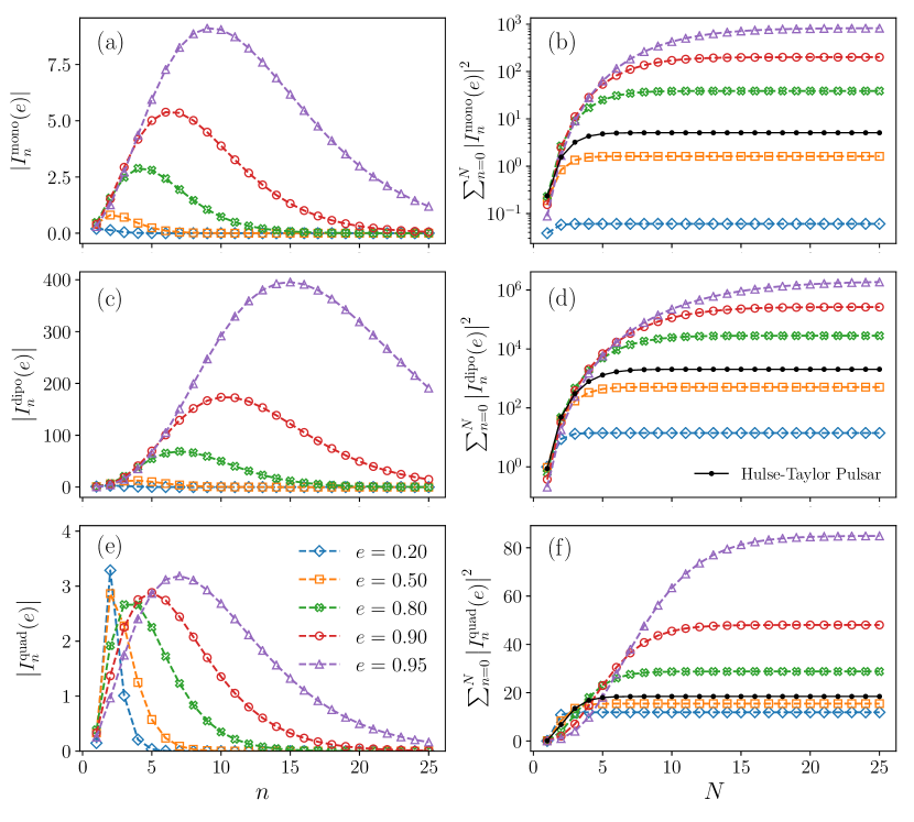
Figure 1: Eccentricity mode functions for the Galileon radiation. The left column of the panels gives the absolute values of $I_{n}^{\rm mono}(e)$, $I_{n}^{\rm dipo}(e)$, and $I_{n}^{\rm quad}(e)$ from top to bottom. The right column of the panels are the cumulative contribution of these functions to the Galileon radiation power, in the form of $\sum_{n=0}^{N}\left|I_{n}^{\rm mono}(e)\right|^{2}$ for the monopole (top), $\sum_{n=0}^{N}\left|I_{n}^{\rm dipo}(e)\right|^{2}$ for the dipole (middle), and $\sum_{n=0}^{N}\left|I_{n}^{\rm quad}(e)\right|^{2}$ for the quadrupole (bottom). Notice that, for clarity panels (b) and (d) have used a logarithmic scale for the vertical axes, while all the other axes are using a linear scale. For a direct check, the solid black lines in the right column of the panels reproduce the result in Figure 1 of de Rham et al. (2013a) for the Hulse-Taylor pulsar PSR B1913+16 whose orbital eccentricity is $e\simeq 0.617$ Weisberg and Huang (2016).

As discussed in the Introduction, (Lorentz invariant) massive gravity models in the decoupling limit essentially reduce to Galileon models plus linearized helicity-2 modes. For the cubic Galileon, we focus on the action Luty et al. (2003); de Rham et al. (2013a),

$$S=\int\mathrm{d}^{4}x\Bigg{[} -\frac{1}{4}h^{\mu\nu}(\mathcal{E}h)_{\mu\nu}+\frac{h^{\mu\nu}T_{\mu\nu}}{2M_{\mathrm{Pl}}}$$

$$~{}~{}-\frac{3}{4}(\partial\pi_{s})^{2}\left(1+\frac{1}{3\Lambda^{3}}\square\pi_{s}\right)+\frac{\pi_{s}T}{2M_{\rm Pl}}\Bigg{]}\,,$$ (10)

where $h_{\mu\nu}\equiv g_{\mu\nu}-\eta_{\mu\nu}$ is the perturbation of the metric, the first two terms in the integrand are the linearized Einstein-Hilbert term coupled to matter with the Lichnerowicz operator $(\mathcal{E}h)_{\mu\nu}\equiv-\frac{1}{2}\square h_{\mu\nu}+\cdots$, $T$ is the trace of the energy-momentum tensor $T^{\mu\nu}$, and $\Lambda$ is the strong coupling scale of the Galileon sector, related to the mass of graviton $m_{g}$ via $\Lambda^{3}=m_{g}^{2}M_{\rm Pl}$. Therefore, the field equations for $\pi_{s}$ and $h_{\mu\nu}$ decouple,

$$\frac{1}{M_{\mathrm{Pl}}}T_{\mu\nu} =-\frac{1}{2}\square h_{\mu\nu}\,,$$ (11)

$$\frac{1}{2M_{\mathrm{Pl}}}T =\partial_{\mu}\left[-\frac{3}{2}\partial^{\mu}\pi_{s}\left(1+\frac{1}{3\Lambda^{3}}\square\pi_{s}\right)+\frac{1}{4\Lambda^{3}}\partial^{\mu}(\partial\pi_{s})^{2}\right]\,.$$ (12)

For a static system whose total mass is $M$, one can define the Vainshtein radius as,

$$r_{\star}=\left(\frac{M}{16m_{g}^{2}M_{\mathrm{Pl}}^{2}}\right)^{1/3}=\frac{1}{\Lambda}\left(\frac{M}{16M_{\mathrm{Pl}}}\right)^{1/3}\,.$$ (13)

Within $r_{\star}$, the fifth force from the scalar degree of freedom is strongly suppressed.

In a static system, the fifth force is suppressed by a factor $\sim\left(L/r_{\star}\right)^{3/2}$, where $L$ is the typical lengthscale of the system Babichev and Deffayet (2013). For example, for an imaginary “static” binary system, we can choose it to be the semimajor axis of the orbit, $L\sim a$. However, binaries are not static. de Rham et al. (2013a) and Chu and Trodden (2013) explicitly worked out the gravitational radiation behaviors in a time-dependent binary system at lowest orders. They found that, (i) extra Galileon radiation powers exist at the monopole, dipole, and quadrupole levels, and (ii) for the dominant radiation the suppression factor is weakened from $\left(L/r_{\star}\right)^{3/2}$ to $\left(n_{b}r_{\star}\right)^{-3/2}$.

Similar to GR, the Newtonian-order contribution of both the monopole and dipole Galileon radiation vanishes, due to the conservation of energy and linear momentum of the system respectively. Post-Newtonian order contributions do exist for them. For the quadrupole radiation, the Newtonian-order contribution is nonzero. We collect the radiation powers of these multiple moments from Ref. de Rham et al. (2013a) (see also the numerical calculation in Ref. Dar et al. (2019)) in the following for later use in this work.

• Monopole radiation. In the cubic Galileon model (II.2), the monopole radiation power at the leading order for a binary system is,

  $${\cal P}_{\rm mono}=\frac{25}{48}\pi\beta^{2}n_{b}^{2}\frac{\left(n_{b}a\right)^{4}}{\left(n_{b}r_{\star}\right)^{3/2}}\frac{M_{\rm mono}^{2}}{M_{\mathrm{Pl}}^{2}}\sum_{n=0}^{\infty}\left|I_{n}^{\rm mono}(e)\right|^{2}\,,$$ (14)

  where the constant $\beta$ and the “monopole mass” $M_{\rm mono}$ (also known as the reduced mass) are defined respectively as,

  $$\beta\equiv\frac{3^{3/8}}{\Gamma(3/4)}\left(\frac{\pi}{32}\right)^{1/4}\simeq 0.6897\,,$$ (15)

  $$M_{\rm mono}\equiv\eta M=\frac{m_{1}m_{2}}{M}\,,$$ (16)

  with $\Gamma(\cdot)$ the gamma function, and the eccentricity mode function $I^{\rm mono}_{n}(e)$ is given in Eq. (24) and Fig. 1.

• Dipole radiation. The dipole radiation power at the leading order for a binary system is,

  $${\cal P}_{\text{ dipole }}=\frac{c_{1}^{2}}{8}n_{b}^{2}\frac{\left(n_{b}a\right)^{6}}{\left(n_{b}r_{\star}\right)^{3/2}}\frac{M_{\rm dipo}^{2}}{M_{\mathrm{Pl}}^{2}}\sum_{n=0}^{\infty}\left|I_{n}^{\rm dipo}(e)\right|^{2}\,,$$ (17)

  where the constant $c_{1}$ and the “dipole mass” are defined respectively as ,

  $$c_{1}\equiv\frac{3^{7/8}\left(\pi/2\right)^{1/4}}{8\,\Gamma(7/4)}\left[1+\frac{3}{16}\frac{\Gamma(7/4)}{\Gamma(11/4)}\right]\simeq 0.4408\,,$$ (18)

  $$M_{\rm dipo}\equiv{\cal X}M_{\rm mono}=M_{\rm mono}\left(\frac{m_{1}-m_{2}}{M}\right)\,,$$ (19)

  where ${\cal X}\equiv\left(m_{1}-m_{2}\right)/M$, and the eccentricity mode function $I_{n}^{\rm dipo}(e)$ is given in Eq. (25) and Fig. 1.

• Quadrupole radiation. Besides the quadrupole radiation power in Eq. (4), the extra power at the leading order reads,

  $${\cal P}_{\rm quad}=\frac{5\lambda^{2}}{32}n_{b}^{2}\frac{\left(n_{b}a\right)^{3}}{\left(n_{b}r_{\star}\right)^{3/2}}\frac{M_{\rm quad}^{2}}{M_{\mathrm{Pl}}^{2}}\sum_{n=0}^{\infty}\left|I_{n}^{\rm quad}(e)\right|^{2}\,,$$ (20)

  where the constant $\lambda$ and the “quadrupole mass” $M_{\rm quad}$ are defined respectively as,

  $$\lambda\equiv\frac{3^{9/8}\pi^{1/4}}{2^{17/4}\Gamma(9/4)}\simeq 0.2125\,,$$ (21)

  $$M_{\rm quad}\equiv{\cal Y}M_{\rm mono}=M_{\rm mono}\left(\frac{\sqrt{m_{1}}+\sqrt{m_{2}}}{\sqrt{M}}\right)\,,$$ (22)

  where ${\cal Y}\equiv\left(\sqrt{m_{1}}+\sqrt{m_{2}}\right)/\sqrt{M}$, and the eccentricity mode function $I_{n}^{\rm quad}(e)$ is given in Eq. (26) and Fig. 1.

The eccentricity mode functions, $I_{n}^{\rm mono}(e)$, $I_{n}^{\rm dipo}(e)$, and $I_{n}^{\rm quad}(e)$, can be defined in a uniform way via the master function,

$$I_{n}^{\left(p,q\right)}(e)\equiv\frac{n^{p+\frac{1}{4}}}{2\pi}\left(1-e^{2}\right)^{p}\int_{0}^{2\pi}\frac{e^{-iqx}}{\left(1+e\cos x\right)^{p}}{\rm d}x\,.$$ (23)

The above mentioned eccentricity functions for monopole, dipole, and quadrupole radiations are,

$$I_{n}^{\rm mono}(e) = I_{n}^{\left(p=2,q=n\right)}(e)\,,$$ (24)

$$I_{n}^{\rm dipo}(e) = I_{n}^{\left(p=3,q=n-1\right)}(e)\,,$$ (25)

$$I_{n}^{\rm quad}(e) = I_{n}^{\left(p=3/2,q=n-2\right)}(e)\,.$$ (26)

The behaviors of these functions are illustrated in Fig. 1 for different values of the eccentricity.

Using the same reasoning of energy balance in Sec. II.1, we can get the extra contributions to $\dot{P}_{b}$ from the extra Galileon radiation powers in Eqs. (14), (17), and (20),

$$\dot{P}_{b}^{\rm mono} =-25\sqrt{2}\beta^{2}\pi^{5/2}\frac{\eta(GM)^{7/6}n_{b}^{1/6}}{\hbar c^{3/2}}\,m_{g}\sum_{n=0}^{\infty}\left|I_{n}^{\rm mono}(e)\right|^{2}\,,$$ (27)

$$\dot{P}_{b}^{\rm dipo} =-6\sqrt{2}c_{1}^{2}\pi^{3/2}\frac{\eta{\cal X}^{2}(GM)^{11/6}n_{b}^{5/6}}{\hbar c^{7/2}}\,m_{g}\sum_{n=0}^{\infty}\left|I_{n}^{\rm dipo}(e)\right|^{2}\,,$$ (28)

$$\dot{P}_{b}^{\rm quad} =-\frac{15}{\sqrt{2}}\lambda^{2}\pi^{3/2}\frac{{\eta\cal Y}^{2}(GM)^{5/6}}{n_{b}^{1/6}\hbar c^{1/2}}\,m_{g}\sum_{n=0}^{\infty}\left|I_{n}^{\rm quad}(e)\right|^{2}\,.$$ (29)

In obtaining these results, at the leading order we have used the Newtonian binding energy for the orbit in Eq. (6), and we have made use of the orbital-averaged radiating powers as discussed above. Such a simplification is sufficient for the analysis in this paper. Notice that the extra contributions to $\dot{P}_{b}$ are all proportional to the graviton mass $m_{g}$, while in the linearized Fierz-Pauli theory Finn and Sutton (2002); Seymour and Yagi (2018); Miao et al. (2019), the extra $\dot{P}_{b}\propto m_{g}^{2}$.

III Constraints from binary pulsars

Now we would like to better understand the physical effect of the Galileon radiation in Eqs. (27–29) to different kinds of binary pulsars. We present some general consideration in Sec. III.1, concerning the dependence on the orbital eccentricity $e$, the orbital period $P_{b}$, and the component masses $\left(m_{1},m_{2}\right)$. We cast constraints on the graviton mass in the cubic Galileon theory from precision timing of fourteen carefully-chosen binary pulsars in Sec. III.2.

III.1 General consideration

From Fig. 1 we see that, (i) given an eccentricity, the absolute values of the eccentricity mode functions, $I_{n}(e)$, increase at first, then have a peak at a particular $n=n^{\rm peak}$ before they decrease; (ii) with the eccentricity increasing, $n^{\rm peak}$ happens at a larger $n$, therefore when we deal with highly eccentric binary pulsars, more modes are to be included in order to guarantee the convergence of the sum; and (iii) the cumulative contributions of these mode functions to the Galileon radiation powers in Eqs. (14), (17), and (20) saturate after a particular $n$, and for $e\lesssim 0.95$, summing up to $N\sim 15$ is generally sufficient. In our following calculation, we choose $N=30$ for a better accuracy. However, one should remember that, for extremely eccentric binaries with $1-e\ll 10^{-2}$, a larger cutoff $N$ is needed.

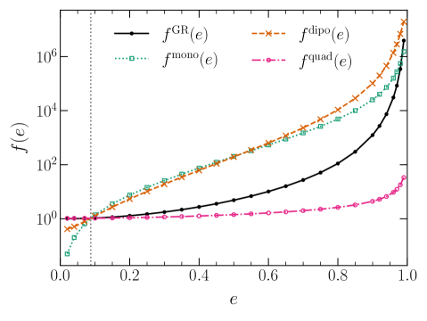
Figure 2: The $f(e)$ factor in $\dot{P}_{b}$, defined in Eqs. (30–33), with a normalization such that $f^{\rm GR}=f^{\rm mono}=f^{\rm dipo}=f^{\rm quad}$ for the double pulsar Kramer et al. (2006) whose $e\simeq 0.088$ (dotted vertical line).

Based on the contribution to the Galileon radiation power, we define,

$$f^{\rm GR}(e) \equiv\left(1+\frac{73}{24}e^{2}+\frac{37}{96}e^{4}\right)\left(1-e^{2}\right)^{-7/2}\,,$$ (30)

and

$$f^{\rm mono}(e) \propto\sum_{n=0}^{\infty}\left|I_{n}^{\rm mono}(e)\right|^{2}\,,$$ (31)

$$f^{\rm dipo}(e) \propto\sum_{n=0}^{\infty}\left|I_{n}^{\rm dipo}(e)\right|^{2}\,,$$ (32)

$$f^{\rm quad}(e) \propto\sum_{n=0}^{\infty}\left|I_{n}^{\rm quad}(e)\right|^{2}\,.$$ (33)

These are the dependence shown in the GR radiation (9) and Galileon radiation (27–29). The proportional factors in Eqs. (31–33) can be arbitrary normalization values for the convenience of specific demonstration.

The $f(e)$ functions in Eqs. (30–33) are plotted in Fig. 2 with a choice of normalization. We can see that the more eccentric binaries are emitting more gravitational waves and contributing more significantly to $\dot{P}_{b}$. This is true for the three types of Galileon radiation, as well as the quadrupole radiation in GR. If the binary is extremely eccentric with $1-e\ll 1$, a huge amplificative factor occurs, especially for the dipole radiation (28) in the cubic Galileon. As we will see below, the quadrupole Galileon radiation is in general the main contributor to $\dot{P}_{b}$ for binaries with comparable component masses de Rham et al. (2013a). The increase of $f^{\rm quad}(e)$ at large eccentricities is slower than the other ones. Notice that the curves in the figure only represent one numerical factor in the radiation power, defined in Eqs. (30–33), while the other dependences (for example, the dependence on the orbital period and the component masses) are omitted here, which will be investigated in the following. Worth to note that, generally the increased radiation due to eccentricity will tend to circularize the orbits (see e.g. in GR Peters and Mathews (1963)), making highly eccentric binaries less likely to exist to date.

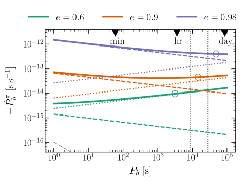
Figure 3: Galileon radiation induced orbital decay as a function of the orbital period $P_{b}$, for three different eccentricities. We have assumed the graviton mass $m_{g}=10^{-27}\,{\rm eV}/c^{2}$, and component masses as per the Hulse-Taylor pulsar, namely $m_{1}=1.438\,M_{\odot}$ and $m_{2}=1.390\,M_{\odot}$. The dotted vertical lines indicate the orbital periods of the double pulsar (left) and the Hulse-Taylor pulsar (right). The dashed, dot-dashed, dotted lines indicate contributions from the monopole, dipole, and quadrupole radiations respectively, while the solid lines are their sum. The dipole radiation is only visible for $e=0.98$ at the bottom left corner of the figure. Open circles on the solid curves represent systems that have lifetime of 1 Myr before merger in GR.

It is interesting to observe that, compared with $\dot{P}_{b}^{\rm GR}/P_{b}\propto n_{b}^{8/3}$ in GR [see Eq. (9)], Galileon radiations have $\dot{P}_{b}^{\rm mono}/P_{b}\propto n_{b}^{7/6}$ [see Eq. (27)], $\dot{P}_{b}^{\rm dipo}/P_{b}\propto n_{b}^{11/6}$ [see Eq. (28)], and $\dot{P}_{b}^{\rm quad}/P_{b}\propto n_{b}^{5/6}$ [see Eq. (29)]. It is a noteworthy feature for the gravitational radiation with the screening mechanism. With such a dependence, while more relativistic binaries are more prominent in emitting gravitational waves in GR, this may not always be true in the cubic Galileon. It resembles the dependence on $n_{b}$ in Lorentz-violating massive gravity Finn and Sutton (2002); Miao et al. (2019) and gravity theories with a time-varying gravitational “constant” $G(t)$ Wex (2014); Seymour and Yagi (2018).

In Fig. 3, we plot three types of Galileon radiation, as function of the orbital period, for a binary pulsar system with component masses similar to the Hulse-Taylor pulsar, and a graviton mass $m_{g}=10^{-27}\,{\rm eV}/c^{2}$. First, we observe that, the dipole radiation is orders of magnitude smaller than the other two types of Galileon radiation, thus it can be totally ignored. Though, as we recall from Fig. 2, the dependence of the $f(e)$ factor for the dipole radiation on the eccentricity $e$ is one of the steepest, the overall effect from dipole radiation is negligible even for $e=0.98$. Then, we observe in Fig. 3 that, while for binaries with $e\lesssim 0.6$, the quadrupole radiation dominates de Rham et al. (2013a), for highly eccentric binaries with relativistic orbits (namely, smaller $P_{b}$), the monopole radiation might dominate instead. This happens when $P_{b}\lesssim 10^{3}\,{\rm s}$ for $e=0.9$, and $P_{b}\lesssim 10^{5}\,{\rm s}$ for $e=0.98$. It is caused by the facts that $\dot{P}_{b}^{\rm mono}$ increases for larger $n_{b}$ (smaller $P_{b}$), while $\dot{P}_{b}^{\rm quad}$ increases for smaller $n_{b}$ (larger $P_{b}$). Therefore, in particular for highly eccentric binaries to be discovered in the future, we should keep in caution of only considering the quadrupole Galileon radiation. This also applies to highly eccentric Galactic binaries (if they exist) in the mHz gravitational-wave band for the Laser Interferometer Space Antenna (LISA) Amaro-Seoane et al. (2017); Barausse et al. (2020). A similar discussion will also be mentioned for pulsar-BH systems in Sec. IV. In our following calculation, we keep all three types of Galileon radiation summed, no matter of their relative strength.

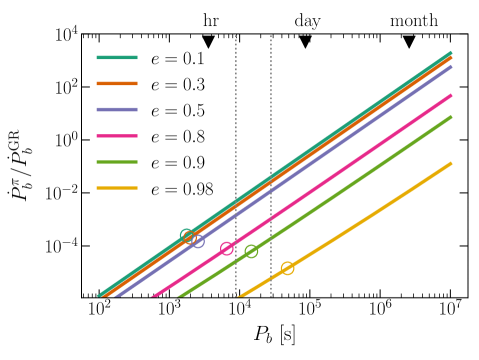
Figure 4: The contribution from the Galileon radiation (summation of the monopole, dipole, and quadrupole radiations), relative to the quadrupole radiation in GR, for several different eccentricities. We have assumed $m_{1}$, $m_{2}$, and $m_{g}$, as per Fig. 3. The dotted vertical lines indicate the orbital periods for the double pulsar (left) and the Hulse-Taylor pulsar (right). Open circles represent systems that have lifetime of 1 Myr before merger in GR.

In Fig. 4, we plot the relative contribution of the Galileon radiation to the quadrupole radiation in GR. First of all, we see that the relative contribution increases when the orbital period is larger. This is in accordance with the screening mechanism which works less well when the size increases Babichev and Deffayet (2013), while the GR effects are more prominent when the orbit is more compact. Specifically it is caused by that, (i) in this regime, the quadrupole Galileon radiation dominates, which increases as $\propto P_{b}^{1/6}$ when $P_{b}$ becomes larger; (ii) the quadrupole radiation in GR decreases as $\propto P_{b}^{-5/3}$. With $m_{g}=10^{-27}\,{\rm eV}/c^{2}$ the Galileon radiation may even be larger than the GR one when $P_{b}\gtrsim{\rm day}$ for nearly circular orbits. Moreover, we find that, while the absolute Galileon quadrupole radiation increases with larger eccentricity (see Fig. 2), the relative contribution to GR decreases. It can be understood from the steepness of the curves in Fig. 2 for the quadrupole radiations in GR (black dots) and in the cubic Galileon (magenta circles). The latter one is less steep, thus decreasing the relative ratio of $\dot{P}_{b}$ with larger eccentricity.

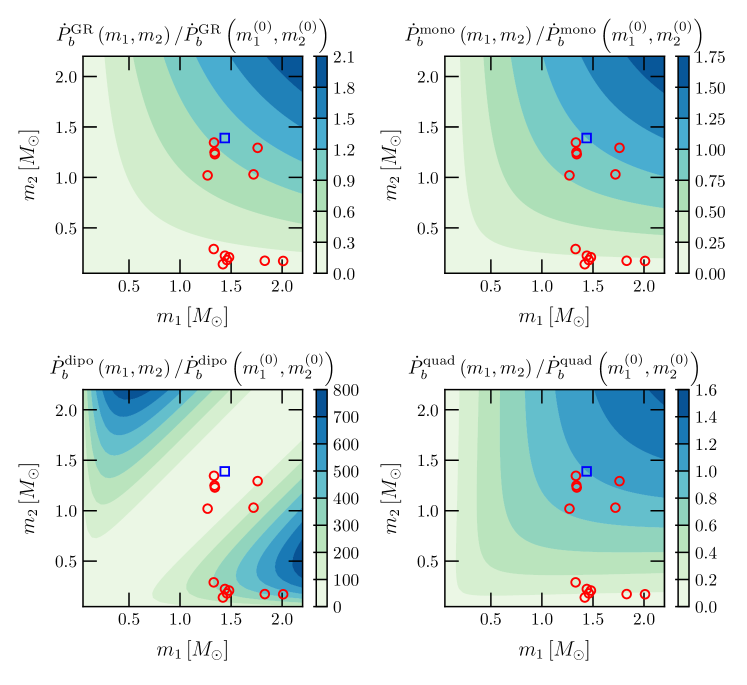
Figure 5: The relative strength to $\dot{P}_{b}$ versus component masses $\left(m_{1},m_{2}\right)$, with given orbital period $P_{b}$ and orbital eccentricity $e$. The panels are for the GR radiation (top left), and monopole (top right), dipole (lower left), quadrupole (lower right) Galileon radiations. The results are calculated with respect to a fiducial mass pair, $m_{1}=1.438\,M_{\odot}$ and $m_{2}=1.390\,M_{\odot}$, denoted by the blue square. Red circles are the other thirteen pulsars that are used in this paper (see Table 1).

Lastly, to understand the effect of component masses, in Fig. 5 we plot the relative strength to $\dot{P}_{b}$ for different mass pairs, normalized to $\left(m_{1},m_{2}\right)=(1.438,1.390)\,M_{\odot}$, which is the fiducial mass pair based on the Hulse-Taylor pulsar Weisberg and Huang (2016). This figure is useful to analyze binaries with given orbital period and eccentricity, but different component masses. It is well known that, for the quadrupole radiation in GR, the so-called chirp mass, ${\cal M}\equiv\left(m_{1}m_{2}\right)^{3/5}/M^{1/5}$, plays the key role, whose contours in the $m_{1}$-$m_{2}$ parameter space are shown in the upper left panel in Fig. 5. The monopole and quadrupole Galileon radiations depend on the component masses in a quantitatively different, but qualitatively similar way, as shown in the right column of panels. But for the dipole radiation, shown in the bottom left panel, the dependence is totally different. Asymmetric binaries are preferred to manifest the dipole radiation. Notice that from the colorbars, the enhancement from asymmetric component masses for the dipole radiation can be as large as $\sim 10^{3}$, while for the other three types of radiation, the change with component masses is within a relatively limited range. This point will be clearly observed for pulsar-BH systems in Sec. IV.

III.2 Constraints

Table 1: Relevant parameters for a collection of binary pulsars to test the Galileon radiation. Component masses were derived using post-Keplerian parameters other than $\dot{P}_{b}$, based on the validity of GR; $\sigma_{\dot{P}_{b}^{\rm obs}}$ is the measurement uncertainty of the timing parameter $\dot{P}_{b}$, while $\sigma_{\dot{P}_{b}^{\rm int}}$ is the uncertainty of $\dot{P}_{b}$ after accounting for the kinematic Shklovskii effect and the Galactic acceleration contribution Damour and Taylor (1991); Lorimer and Kramer (2005). Parenthesized numbers represent the 1-$\sigma$ uncertainty in the last digit(s) quoted. For more details, interested readers are referred to the cited references alongside the pulsar name for each pulsar.

Pulsar	$P_{b}\,[{\rm d}]$	$e$	$m_{1}\,[M_{\odot}]$	$m_{2}\,[M_{\odot}]$	$\sigma_{\dot{P}_{b}^{\rm obs}}\,[{\rm s\,s}^{-1}]$	$\sigma_{\dot{P}_{b}^{\rm int}}\,[{\rm s\,s}^{-1}]$
J0348+0432 Antoniadis et al. (2013)	0.102424062722(7)	$(2.6\pm 0.9)\times 10^{-6}$	2.01(4)	0.172(3)	$4.5\times 10^{-14}$	$4.5\times 10^{-14}$
J0437$-$4715 Reardon et al. (2016); Perera et al. (2019)	5.7410458(3)	$1.9182(1)\times 10^{-5}$	1.44(7)	0.224(7)	$3\times 10^{-15}$	$2.8\times 10^{-13}$
J0613$-$0200 Desvignes et al. (2016); Perera et al. (2019)	1.198512575217(10)	$4.50(9)\times 10^{-6}$	1.42(46)	0.14(3)	$7\times 10^{-15}$	$2.3\times 10^{-14}$
J0737$-$3039A Kramer et al. (2006); Kramer (2016)	0.10225156248(5)	0.0877775(9)	1.3381(7)	1.2489(7)	$1\times 10^{-15}$	$1\times 10^{-15}$
J1012+5307 Lazaridis et al. (2009); Perera et al. (2019)	0.604672723085(3)	$(1.1\pm 0.1)\times 10^{-6}$	1.83(11)	0.174(7)	$4\times 10^{-15}$	$8\times 10^{-15}$
J1022+1001 Desvignes et al. (2016); Perera et al. (2019)	7.805136(1)	$9.704(5)\times 10^{-5}$	1.72(65)	1.03(36)	$7\times 10^{-14}$	$2\times 10^{-13}$
J1141$-$6545 Bhat et al. (2008); Krishnan et al. (2020)	0.19765096149(3)	0.171876(1)	1.27(1)	1.02(1)	$2.5\times 10^{-14}$	$2.5\times 10^{-14}$
B1534+12 Fonseca et al. (2014)	0.420737298879(2)	0.27367752(7)	1.3330(2)	1.3455(2)	$3\times 10^{-16}$	$1.1\times 10^{-14}$
J1713+0747 Zhu et al. (2019); Perera et al. (2019)	67.8251299228(5)	$7.49403(7)\times 10^{-5}$	1.33(10)	0.290(11)	$1\times 10^{-13}$	$1\times 10^{-13}$
J1738+0333 Freire et al. (2012)	0.3547907398724(13)	$(3.4\pm 1.1)\times 10^{-7}$	$1.46(6)$	$0.181(8)$	$3.1\times 10^{-15}$	$3.2\times 10^{-15}$
J1756$-$2251 Ferdman et al. (2014)	0.31963390143(3)	0.1805694(2)	1.341(7)	1.230(7)	$5\times 10^{-15}$	$8\times 10^{-15}$
J1909$-$3744 Desvignes et al. (2016); Perera et al. (2019)	1.533449475278(1)	$1.04(6)\times 10^{-7}$	1.48(3)	0.209(1)	$3\times 10^{-15}$	$1.4\times 10^{-14}$
B1913+16 Weisberg and Huang (2016)	0.322997448918(3)	0.6171340(4)	1.438(1)	1.390(1)	$1\times 10^{-15}$	$4\times 10^{-15}$
J2222$-$0137 Cognard et al. (2017)	2.44576456(13)	$0.380940(3)\times 10^{-4}$	1.76(6)	1.293(25)	$9\times 10^{-14}$	$9\times 10^{-14}$

After having looked at the general features for the Galileon radiation in the last subsection, now we turn to realistic binary pulsar systems. We carefully choose fourteen binary pulsars that are known to be precisely timed. They are chosen from the pool of millisecond pulsars in the second Data Release of the International Pulsar Timing Array program Perera et al. (2019), as well as several other well-known systems with measurement of $\dot{P}_{b}$ Antoniadis et al. (2013); Reardon et al. (2016); Desvignes et al. (2016); Kramer et al. (2006); Kramer (2016); Lazaridis et al. (2009); Bhat et al. (2008); Krishnan et al. (2020); Fonseca et al. (2014); Zhu et al. (2019); Freire et al. (2012); Ferdman et al. (2014); Weisberg and Huang (2016); Cognard et al. (2017). The relevant parameters for the test of the Galileon radiation are listed in Table 1. Because binary pulsars have a large variety in terms of system parameters and observational characteristics, for detailed description of these systems, readers are referred to the original timing papers which are given for each pulsar in the table. As one can see from the last subsection, the Galileon radiation depends on a set of physical parameters of the binary pulsar system. These pulsars in Table 1 represent, to our best knowledge and resource, a set of the most suitable binary pulsar systems to date to perform the test in this paper.

For the chosen binary pulsars, post-Keplerian parameters, other than $\dot{P}_{b}$, were used to calculate the component masses $m_{1}$ and $m_{2}$, assuming the validity of GR expressions Lorimer and Kramer (2005); Wex (2014). The component masses are listed in the fourth and fifth columns in Table 1. In the strictest sense, the component masses should be calculated consistently using cubic Galileon theory instead of GR. Nevertheless, as the Vainshtein suppression of the fifth force is more significant than the Galileon radiation de Rham et al. (2013a, b), it is safe to use the GR formulae to extract these parameters.

As we can see in the penultimate column in the table, most of the chosen pulsars have uncertainties for the value of measured $\dot{P}_{b}$ at the level of $\sigma_{\dot{P}_{b}^{\rm obs}}\sim 10^{-15}\,{\rm s\,s}^{-1}$. PSR B1534+12 has an even better measurement with $\sigma_{\dot{P}_{b}^{\rm obs}}\simeq 3\times 10^{-16}\,{\rm s\,s}^{-1}$ Fonseca et al. (2014). The excellent timing precision is attributed to the long-term observation of these pulsars and the continuous improvements of the instruments at large radio telescopes Lorimer and Kramer (2005); Kramer et al. (2004); Shao et al. (2015). However, these values cannot be directly used due to the astrophysical contribution and imperfect knowledge about their distances as well as the Milky Way’s gravitational potential Damour and Taylor (1991); Lorimer and Kramer (2005). The most significant contribution comes from the kinematic Shklovskii effect and the Galactic acceleration contribution. These contributions need to be subtracted using the measurement of the proper motion and the modeling of the Galactic potential Damour and Taylor (1991). The subtraction introduces extra uncertainties in the intrinsic $\dot{P}_{b}$ parameter. The uncertainty after the subtraction, denoted as $\sigma_{\dot{P}_{b}^{\rm int}}$, is listed in the last column of Table 1 for each pulsar.

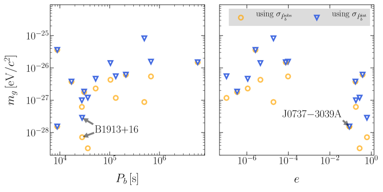
Figure 6: Constraints on the graviton mass in cubic Galileon theory from individual binary pulsars versus their orbital periods (left) and eccentricities (right) at 68% C.L.. Orange circles and blue triangles are bounds obtained using $\sigma_{\dot{P}_{b}^{\rm obs}}$ and $\sigma_{\dot{P}_{b}^{\rm int}}$, respectively. The Hulse-Taylor pulsar PSR B1913+16 Weisberg and Huang (2016) and the double pulsar PSR J0737$-$3039A Kramer (2016) are annotated.

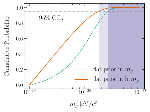
Figure 7: Cumulative probability for the graviton mass with flat priors in $m_{g}$ (dashed) and $\ln m_{g}$ (solid). Shaded regions show the excluded graviton mass values at 95% C.L. [see Eq. (35) and Eq. (36)].

All the pulsars in the table have passed the tests of GR Wex (2014). In particular, the measured orbital decay rates, after subtracting the kinematic Shklovskii effect and the Galactic acceleration contribution, agree with the GR prediction in Eq. (9) within uncertainty for all binary pulsars that we consider. Therefore, here we do not look for evidence of the Galileon radiation, instead we put upper bounds on the graviton mass via constraining the extra Galileon radiation. By plainly assuming that the Galileon radiation is smaller than the uncertainty in $\dot{P}_{b}$, we obtain upper bounds for the graviton mass for each pulsar. These bounds are plotted in Fig. 6 for cases using $\sigma_{\dot{P}_{b}^{\rm int}}$ and $\sigma_{\dot{P}_{b}^{\rm obs}}$, as function of the orbital period $P_{b}$ and the orbital eccentricity $e$.

The scenario of using $\sigma_{\dot{P}_{b}^{\rm int}}$ should be taken as providing the current bounds on $m_{g}$. In this scenario, the best bound is given by the agreement of $\dot{P}_{b}$ to the GR prediction within $10^{-3}$ from the recent observation of the double pulsar PSR J0737$-$3039A Kramer (2016). The bound on $m_{g}$ reads,

$$m_{g}\lesssim 3\times 10^{-28}\,{\rm eV}/c^{2}\quad\mbox{(95\% C.L.)}\,,$$ (34)

which is two times better than the bound from the Hulse-Taylor pulsar PSR B1913+16, which gives $m_{g}\lesssim 6\times 10^{-28}\,{\rm eV}/c^{2}$ (95% C.L.) Weisberg and Huang (2016). Although the larger eccentricity of PSR B1913+16 ($e\simeq 0.617$) is beneficial to the test, compared with a mildly small eccentricity for PSR J0737$-$3039A ($e\simeq 0.088$), the astrophysical contribution introduces a significant uncertainty to the intrinsic $\dot{P}_{b}$ of PSR B1913+16 Damour and Taylor (1991). The double pulsar, being relatively close to the Earth, is not yet limited by the astrophysical contribution in $\dot{P}_{b}$ Kramer et al. (2006).

The scenario of using $\sigma_{\dot{P}_{b}^{\rm obs}}$, on the other hand, should be taken as over-optimistic, representing the ability of clean binary pulsar systems in constraining the graviton mass. This is only possible when the kinematic Shklovskii effect is measured and the Galactic acceleration is modeled both to be better than the observational uncertainty. In such an idealized case, the best pulsar would be PSR B1534+12 Fonseca et al. (2014), which gives $m_{g}\lesssim 6\times 10^{-29}\,{\rm eV}/c^{2}$ (95% C.L.) by itself alone. These over-optimistic results are also plotted in Fig. 6 with orange circles, but they are only considered to be indicative of technology capability and not used in the following analysis.

Because the theory parameter, $m_{g}$, is universal to different pulsars, we can combine the constraints from individual pulsars into a combined constraint. We assume that the measurements for different binary pulsars are independent, thus the covariant matrix is diagonal for them. We make use of a simple (logarithmic) likelihood $\ln{\cal L}\equiv-\frac{1}{2}\sum_{i}\big{(}\dot{P}_{b}^{\pi}/\sigma_{\dot{P}_{b}^{\rm int}}\big{)}^{2}$, where $\dot{P}_{b}^{\pi}$ is a sum of Galileon radiations in Eqs. (27–29), $\sigma_{\dot{P}_{b}^{\rm int}}$ is given in Table 1, and the summation is over all binary pulsars considered in this paper. We can also assign prior knowledge to the graviton mass within the framework of Bayesian statistics Del Pozzo and Vecchio (2016). In Fig. 7 we plot the combined cumulative probability distribution of the graviton mass for two different sets of prior knowledge. The combined bound is dominantly influenced by PSRs J0737$-$3039A and B1913+16, while the other twelve pulsars only play a minor role. From the figure, we obtain

$$m_{g}\lesssim 3\times 10^{-28}\,{\rm eV}/c^{2}\quad\mbox{(95\% C.L.)}\,,$$ (35)

when a uniform prior on $m_{g}\in(10^{-29},10^{-27})\,{\rm eV}/c^{2}$ is assumed, and

$$m_{g}\lesssim 2\times 10^{-28}\,{\rm eV}/c^{2}\quad\mbox{(95\% C.L.)}\,,$$ (36)

when a uniform prior on $\ln m_{g}$ for $m_{g}\in(10^{-29},10^{-27})\,{\rm eV}/c^{2}$ is assumed; the high end of the prior range, namely $10^{-27}\,{\rm eV}/c^{2}$, comes from the analysis in Ref. de Rham et al. (2013a). While the former bound (35) is very robust, the latter bound (36) using a uniform prior on $\ln m_{g}$ depends on our choice of prior range. It is a generic feature of Bayesian analysis. In a cosmologically favored reasoning, one might expect the graviton mass to be around the current Hubble scale, namely $m_{g}\sim H_{0}\sim 10^{-33}\,{\rm eV}/c^{2}$. If we had used a uniform prior on $\ln m_{g}$ for $m_{g}\in(10^{-34},10^{-27})\,{\rm eV}/c^{2}$, we would have obtained a much tighter bound of $m_{g}$. However, such a bound is dominated by the prior knowledge. It means that binary pulsars are not yet sensitive to a cosmologically small graviton mass. Therefore, we stick to our relatively conservative result in Eq. (36). In contrast, the above change in the prior range does not affect the bound in Eq. (35) when a uniform prior on $m_{g}$ is adopted.

The results on $m_{g}$ here improve the one in Ref. de Rham et al. (2013a), $m_{g}\lesssim 10^{-27}\,{\rm eV}/c^{2}$ (95% C.L.), due to the use of an updated analysis and the use of recent observational results of pulsar timing, in particular the use of the double pulsar results given in Ref. Kramer (2016).

IV Projected constraints with pulsar-BH systems

A well-timed pulsar around a BH companion is a long-sought holy grail in the pulsar astronomy. The discovery of these systems will enable a couple of unprecedented tests of gravity theories, in particular on the aspects related to the property of BH solutions Wex and Kopeikin (1999); Kramer et al. (2004); Shao et al. (2015, 2018); Seymour and Yagi (2018); Weltman et al. (2020). Up to now, despite extensive dedicated searches, no conclusively convincing candidate has been found. The uncertainty in the estimation of the number of these potential systems pertains mainly to their formation channels. We will not discuss further the involved astrophysics here. Nevertheless, several studies have shown a good potential for the discovery of pulsar-BH systems in the near future Liu et al. (2012); Wharton et al. (2012); Liu et al. (2014); Bower et al. (2018, 2019). If such a pulsar-BH system is discovered, it will provide a completely new playground to perform interesting tests of gravity, including the Galileon radiation Seymour and Yagi (2018).

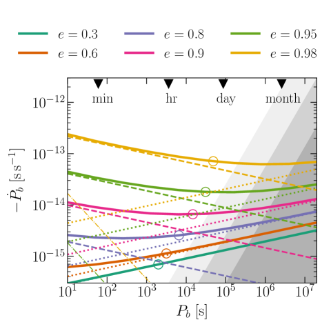
Figure 8: Same as Fig. 3, but for $m_{1}=1.4\,M_{\odot}$, $m_{2}=10\,M_{\odot}$, and $m_{g}=10^{-28}\,{\rm eV}/c^{2}$. Open circles represent systems that have lifetime of 1 Myr before merger in GR. Shaded regions show the estimated measurement precision that can be achieved with (from dark to light) $\sigma_{\rm TOA}=0.1\,\mu$s, $1\,\mu$s, and $10\,\mu$s; the precision is found to be independent of eccentricity. Note that our simulations are performed for orbits with $P_{b}\gtrsim 0.2\,$day, and in this figure orbits with $P_{b}\lesssim 0.2\,$day are extrapolated with Eq. (37).

In Fig. 8, we plot the expected contribution from the Galileon radiation to the orbital decay rate for a pulsar – $10\,M_{\odot}$ BH system. In this figure, the graviton mass is assumed to be $m_{g}=10^{-28}\,{\rm eV}/c^{2}$, which is roughly the best bound from the combination of the current binary pulsars, obtained in Eqs. (35) and (36). Because of the asymmetric masses, for extreme (unrealistic) systems with $P_{b}\lesssim 1\,{\rm minute}$ and $e\gtrsim{0.95}$, the Galileon dipole radiation could be relevant to the total radiation. However, even if there exist such kind of systems, they are unlikely to be detected with radio telescopes due to the large orbital acceleration and limited computation resources Liu et al. (2014); however, fast imaging and imaging searches based on significant circular polarization or scintillation might help Law et al. (2018); Kaplan et al. (2019); Dai et al. (2016). The expected number for the LISA detector is very low as well, due to their short lifetime before the merger Amaro-Seoane et al. (2017). For binaries with $P_{b}\gtrsim 1\,{\rm day}$, the Galileon quadrupole radiation is still the dominant contributor.

Depending on the eccentricity, now the Galileon monopole radiation could play an essential role for binaries with $P_{b}\lesssim 1\,{\rm day}$. Discovery of such binaries might be realistic for current and upcoming radio telescopes Kramer et al. (2004); Liu et al. (2014). Liu et al. (2014) conducted extensive time-of-arrival (TOA) simulation for a pulsar-BH system with masses $\left(m_{1},m_{2}\right)=\left(1.4,10\right)\,M_{\odot}$.

Similar to Ref. Liu et al. (2014), we have conducted extensive mock-data simulations, for different pulsar-BH configurations. For all these simulations we have assumed one observing session per week with ten TOAs of given uncertainty $\sigma_{\rm TOA}$, over a period of five years. We further assume that the TOAs follow a Gaussian distribution and are uncorrelated (white noise). Our simulations cover an orbital period range from 0.2 to about 100 days. We find that, with given orbital period, the precision in measuring $\dot{P}_{b}$, denoted by the (dimensionless) quantity $\sigma_{\dot{P}_{b}}$, is only weakly dependent on the orbital eccentricity. The dependence on $P_{b}$ is nicely fitted by,

$$\log_{10}\sigma_{\dot{P}_{b}}={\cal A}+{\cal B}\log_{10}\left(\frac{P_{b}}{\rm day}\right)\,,$$ (37)

where $({\cal A},{\cal B})=(-15.67,1.331)$, $(-14.67,1.331)$, and $(-13.68,1.332)$, when $\sigma_{\rm TOA}$ is $0.1\,\mu$s, $1\,\mu$s, and $10\,\mu$s, respectively. In fact, to good approximation one can use ${\cal A}=-14.7+\log_{10}\left(\sigma_{\rm TOA}/\mu{\rm s}\right)$ and ${\cal B}=1.33$. The actual uncertainty obtained for a TOA depends on various aspects, like pulsar luminosity, pulse profile, integration time, telescope and backend parameters, etc. The assumed uncertainties and number of TOAs are typical for precision timing observations in pulsar astronomy (see e.g. Ref. Perera et al. (2019)). The expected precision for the three different values of $\sigma_{\rm TOA}$ is shown as shaded regions in Fig. 8. We see that pulsar-BH systems will have a great potential to improve the current best bound on $m_{g}$. For example, if $\sigma_{\rm TOA}$ about $0.1\,\mu$s ($10\,\mu$s) is achieved, an eccentric pulsar with $P_{b}\lesssim 1$ month ($P_{b}\lesssim 1$ day) can probe $m_{g}$ down to the level of $10^{-28}\,{\rm eV}/c^{2}$. We would like to emphasise that the timing precision assumed here can generally only be achieved for recycled pulsars, even with large radio telescopes like the Five-hundred-meter Aperture Spherical Telescope (FAST) Jiang et al. (2019); Lu et al. (2019) or the upcoming Square Kilometre Array (SKA) Kramer et al. (2004); Shao et al. (2015); Weltman et al. (2020). Such pulsar-BH systems could in principle be the result of an exchange encounter in regions with high stellar density, like globular clusters and the Galactic centre region (see e.g. Ref. Faucher-Giguère and Loeb (2011)). The actual timing precision will, in addition, depend on other parameters like pulsar luminosity, pulse shape, etc.

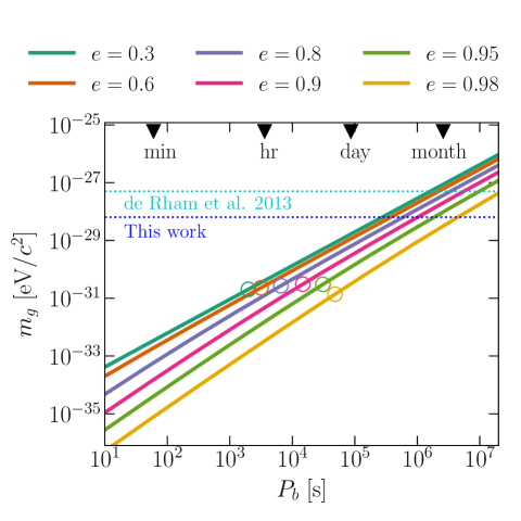
Figure 9: Projected bounds at 68% C.L. on $m_{g}$ from a pulsar-BH system with $\sigma_{\rm TOA}=0.1\,\mu$s. Open circles represent systems that have lifetime of 1 Myr before merger in GR. As in Fig. 8, results for orbits with $P_{b}\lesssim 0.2\,$day are extrapolated via Eq. (37).

In Fig. 9, we plot the projected bounds on $m_{g}$ using the $\dot{P}_{b}$ precision in Eq. (37) with $\sigma_{\rm TOA}=0.1\,\mu$s. As we can see from the figure, if we can time a near-circular pulsar-BH binary with $P_{b}$ smaller than a few days, the bound (36) in this paper can be improved. If the binary is highly eccentric, then an orbital period $P_{b}$ smaller than a few months is sufficient to improve the bound, as was indicated in Fig. 8. On the other hand, if one wants to probe the cosmologically interested range for $m_{g}\sim 10^{-33}\,{\rm eV}/c^{2}$ de Rham et al. (2013a), a sub-minute circular binary, or a sub-hour highly eccentric binary, is needed. We consider such cases highly unlikely to be discovered with near-future technologies, leaving aside the fact that the existence of such a system in our Galaxy is almost certainly excluded, due to its short merger time.

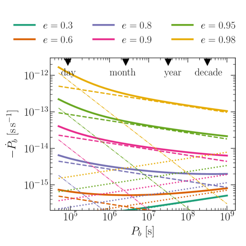
Figure 10: Same as Fig. 3, but for $m_{1}=1.4\,M_{\odot}$, $m_{2}=4\times 10^{6}\,M_{\odot}$, and $m_{g}=10^{-28}\,{\rm eV}/c^{2}$.

In another direction, extensive searches for pulsars around the Sgr A^∗, the supermassive BH at the centre of our Galaxy, are ongoing Liu et al. (2012); Bower et al. (2018, 2019); Goddi et al. (2016). In Fig. 10 we plot the Galileon radiation for a pulsar – Sgr A^∗ BH system for different eccentricities with $m_{g}=10^{-28}\,{\rm eV}/c^{2}$. For eccentric systems with $P_{b}\lesssim 1\,{\rm yr}$, the Galileon monopole radiation prevails over the Galileon quadrupole radiation for $e\gtrsim{0.6}$. Therefore, there might be an opportunity to test the Galileon monopole radiation within this class of systems. To address this question, we perform mock-data simulations to investigate the precision one can expect for $\dot{P}_{b}$ for a pulsar in a suitable orbit around Sgr A*. Similar to Ref. Liu et al. (2012), we have created mock data with one TOA of 100 $\mu$s precision every week, over a time span of five years. Furthermore, we have assumed that the pulsar orbit is unperturbed and therefore our parameter estimation is based on a phase-connected timing solution that provides a perfect fit over the whole time span of observations. Even under such optimistic assumptions, we find that, for an orbit with $P_{b}=0.5\,$yr and $e=0.8$, it is unlikely to get a $\sigma_{\dot{P}_{b}}$ better than $10^{-12}\,{\rm s\,s}^{-1}$. Therefore, only in the event of a pulsar in a highly eccentric orbit with $P_{b}\lesssim 1\,$day being discovered, we might be able to improve the bound (36). However, we consider the existence of a pulsar in such an orbit extremely unlikely.

The tests in this section depend sensitively on the actual eccentricity of the pulsar-BH system, as shown in the Figs. 8–10. In fact, the analysis with Fig. 8 and Fig. 10 is conservative, because the Galileon radiation power was calculated averaging over the orbital timescale de Rham et al. (2013a). In reality, during the periastron passage the gravitational radiation will be maximized, and produce prominent features. These features are believed to provide even better distinguishable signals. An analysis resolving the orbital timescale is beyond the scope of this paper. Because all three kinds of the Galileon radiations are proportional to $m_{g}$, the results discussed in Fig. 8 and 10 can be rescaled easily with different graviton mass for different binary systems.

V Discussion

In this paper we systematically studied the Galileon radiation in cubic Galileon theory de Rham et al. (2013a) in the context of pulsar timing. Because the Galileon radiation is screened differently than its fifth-force counterpart, such a study is essential to better understand the basic role of the Vainshtein mechanism in screening the gravitational radiation.

From a collection of fourteen well-timed binary pulsars, we have obtained a new bound on the theory parameter for cubic Galileon, namely the graviton mass,

$$m_{g}\lesssim 2\times 10^{-28}\,{\rm eV}/c^{2}\quad\mbox{(95\% C.L.)}\,,$$ (38)

when a uniform prior on $\ln m_{g}$ for $m_{g}\in(10^{-29},10^{-27})\,\mathrm{eV}/c^{2}$ is used. This improves a previous bound from the Hulse-Taylor pulsar de Rham et al. (2013a) by a factor of five. Though the bound (38) is weaker than a few other bounds such as bounds from the Earth-Moon-Sun system and dark matter clusters de Rham et al. (2017), it is nevertheless a robust bound from a completely different regime, namely from the dynamic gravitational radiation instead of the static environments. It is also immune from uncertain assumptions about the dark matter distributions and the virialization of the gravitating systems. Therefore, we consider this bound complementary to the existing bounds.

Finally, de Rham et al. (2013b) have discussed radiations from a generic Galileon theory with all allowed interactions in the 4-dimensional spacetime. The inclusion of quartic or quintic Galileon complicates the calculations considerably. The authors found that, the naive perturbation theory predicts divergent results in the radiation power when these higher-order terms are considered, meaning that the perturbations themselves are nonlinear. Partial results were obtained for binary systems with specific assumptions about the screening lengthscales. In particular, only circular binary orbits were analyzed, thus not applicable to most of the systems that we consider in this paper. For circular orbits that were considered in Ref. de Rham et al. (2013b), meaningful bounds can be derived when there is a hierarchy of strong coupling scales. We wish to perform a more complete analysis with higher-order Galileon interactions in a future study.