On Optimal Placement of Hybrid Service Function Chains (SFCs) of Virtual Machines and Containers in a Generic Edge-Cloud Continuum

Abstract

Traditionally, Network Function Virtualization (NFV) has been implemented to run on Virtual Machines (VMs) in form of Virtual Network Functions (VNFs). More recently, the so-called Serverless Computing has gained traction in cloud computing, offering Function-as-a-Service (FaaS) platforms that make use of containerization techniques to deploy services. In contrast to VM-based VNFs, where resources are usually reserved and continuously running, FaaS can just be subsets of code implementing small functions allowing for event-driven, on-demand instantiations. Thus, a hybrid VM-Container based Service Function Chains (SFCs) are a natural evolution of NFV architecture. We study a novel problem of optimal placement of hybrid SFCs from an Internet Service Provider (ISP) point of view, whereby VNFs can be instantiated either over VMs or containers in a generic edge and cloud continuum. To this end, we propose a Mixed-Integer Linear Programming model as well as a heuristic solution to solve this optimization problem that considers three objectives unique to the specific VM and container deployment in a carrier network: operational costs for maintaining servers in the edge, costs of placing VNFs in third-party cloud providers and penalty costs applied when SLA agreements are violated in terms of end-to-end delay. We also propose 2-phases optimization process to analyze the effect on performance as a result of replications and migrations of VNFs. The model can be used to highlight scenarios where a combination of VMs and containers can provide most benefits from the monetary costs point of view.

I Introduction

Internet Service Providers (ISP) recognize Network Function Virtualization (NFV) as a key concept to reducing capital and operational expenditures (Capex and Opex). In NFV, Virtual Network Functions (VNFs) run over Virtual Machines (VMs) that are managed in the Network Function Virtualization Infrastructure (NFVI) by the NFV Management and Orchestrator module (NFV MANO)[1]. Full service provisioning is achieved by concatenating multiple VNFs in an specific sequence order, defined as Service Function Chains (SFCs). The placement of chained VNFs into physical servers, known as VNF placement problem, can follow different optimization objectives, such as network load balancing, reliability, end-to-end delay, etc. More recently, NFV concept has further evolved towards the so-called Serverless Computing, adopting Function-as-a-Service (FaaS) technology as a way to also deploy VNFs over containers, with AWS Lambda being the first public cloud Infrastructure to offer these services in 2014 [2]. To further reduce Opex, it is expected that traditional VM-based VNFs (VM-VNFs) are going to co-exist with container-based VNFs (CT-VNFs) under the same management system. The Open Source Mano (OSM) is already supporting the integration of Virtual Infrastructure Managers (VIMs), a serverless platform that can integrate VNFs, such as OpenWhisk [3].

So far, little is known about placement of VNFs that run over containers (CT-VNFs), and especially when chained together with VMs in an SFC. From the point of view of the server utilization, VM-VNFs require much more server resources compared to CT-VNFs, due to the overhead introduced by the hypervisor-based virtualization technology. From the OPEX point of view, CT-VNFs deployed on third party cloud services are more expensive as they are usually charged by usage, as opposed to VMs that typically have fixed cost rates by deployment. Furthermore, NFV can make use of migrations and replications of VNFs, for instance, to adapt to service request variability, to increase quality of service (QoS), reliability, etc. While migrations are known to increase the probability of violating SLAs due to service interruptions incurring into penalty costs for the ISP, replications require extra server and network resources due to the overhead and state synchronization. If an ISP needs to rent resources from a cloud provider, on the other hand, the choice between VM-VNFs and CT-VNFs has direct impact on the costs to pay due to the different charging rates of a cloud provider. Thus, the optimization of VM-VNFs and CT-VNFs placement presents a few important and interesting challenges which have not been solved yet. This is especially interesting to solve in an ISP-centric model of edge-to-cloud continuum, where it can be differentiated between the costs associated with the edge network and the cloud considering that the ISP owns the edge infrastructure and is charged when using a third-party cloud.

In this paper, we propose a Mixed-Integer Linear Programming (MILP) model to study the placement optimizations of VMs and containers in hybrid SFC configurations in a generic ISP-centric model of edge-cloud continuum. We propose to solve the VNF placement problem in two phases, starting off with low traffic load and solving the placement problem under high traffic load. We use the low traffic phase as an initial placement to understand the effects in the second phase of, from one side, migrations (that have on the penalty costs caused by service interruptions) and, on the other side, replications (that impact the network and server resources due to state synchronization tasks). To this end, we define a joint optimization problem with three different costs models for the ISP: (i) operational costs for maintaining servers in the edge network, (ii) charges applied when the service provider uses a third party cloud provider, and (iii) penalty costs applied for SLA violations. In contrast to other placement models based on variants of well-known multi-commodity flow problem, our model optimally uses multiple traffic flows in SFCs, and unlike any known SFC multipath model that only restrict the propagation delay of all predefined paths or use the end-to-end delay simply averaged over paths, our model considers individual end-to-end delays for each traffic flow. We also propose a greedy algorithm as an online solution that performs close to the optimal solution. The results show the performance and the related cost-tradeoffs of hybrid SFC deployment.

The rest of the paper is organized as follows. Section II presents related work. Section III describes the system model. Section IV formulates the optimization model. Section V describes the heuristics. Section VI analyzes the performance and Section VII concludes the paper.

II Related Work and Our Contribution

II-A VNF placement, migrations and replications

Significant amount of previous work has focused on the VNF placement problem considering VMs as underlying technology. More in detail, VM-VNFs placement problem has been addressed by the research community with variants of the joint optimization placement problem with different objectives. For instance, in [4], a resource allocation solution is proposed for optimizing energy efficiency, while considering delay, network and server utilization. [5] proposes a joint optimization solution, considering network and service performance, to not only solve the VNF placement problem, also known as Forwarding Graph Embedding, but also the VNF Chain Composition and VNFs scheduling problems. [6] proposed models to finding the optimal dimensioning and resource allocation with latency constraints in mobile networks.

Whereas no distinctive challenges have been reported between VMs and container placement [7], considering migrations and replication, the two concepts exhibit more features that need to be differentiated. In case of VM-VNFs, and under certain circumstances, migration is required, which can be implemented either by migrating the entire VM [8] or by migrating only the internal states of an VNF [9]. Accordingly, multiple objectives can be applied, such as minimizing the impact on QoS, maximizing the energy efficiency, maximizing load balancing, etc (e.g. [10], [11] and [12]). In this regard, it has been reported that the migration process can be up to four times faster with containers than when using VMs [13]. Since the main issue with VM-VNFs migrations is the problem of service interruptions that negatively impact QoS, previous work, e.g., [14] derived a trade-off between the power consumption and QoS degradation to determine whether a migration is appropriate. On the other hand, VM-VNFs replications (sometimes also referred as backups) have been primarily used to provide service reliability [15] while trying to minimize the number of required replicas [16], to reduce end-to-end service delays [17] [18], to load balance the link utilization [19] and to load balance the server utilization [20]. While in a related work in [21], the authors try to balance the number of migrations and replications in order to maximize the network throughput and minimize the end-to-end delay, in [22] the objective is to reduce migrations by using replications to find a trade-off between both mechanisms to improve server, network load balancing and QoS. In this regard, when using containers to create VNF replicas, it is proven that they can reduce instantiation delay and to increase throughput while achieving near zero downtime of the SFC [23].

II-B Edge-Cloud Continuum and the Issues of Placement

The emerging edge computing trend is looking at distributing computation resources closer to the network users in order to minimize end-to-end latencies and to reduce the transit traffic in the core network. In these highly distributed edge scenarios, where the computing capabilities are typically more constrained than in the cloud, the standard full MANO stack is not suitable. Instead, new solutions propose the usage of lightweight virtualization platforms using containerization techniques as a solution for orchestration and management of network services [24], [25] and for the deployment of VNFs achieving very low resource usage overhead, almost comparable to bare metal [26]. The latest developments in the Open Source Mano already include support not only for virtual, physical and hybrid network functions (VNFs, PNFs and HNFs, respectively), but also to Virtual Infrastructure Managers (VIMs) and WAN Infrastructure Managers (WIMs) [27]. One of the recent projects making use of the VIM support integrates Apache OpenWhisk which has support to FaaS, through the development of a VIM plugin [3]. In this context, more recent studies, e.g., [28], analyze the VNF placement at the edge in order to improve QoS by constraining the maximum number of SLA violations in terms of end-to-end latency, which is the salient feature of edge computing. In [29], a management mechanism is proposed, based on NFV/SDN ISP networks to provide multicast edge-based services. Similarly, in [30], a deployment model of VNFs is presented with location-awareness to meet the QoS in mobile networks.

II-C Our Contribution

Motivated by the fact that NFV-enabled edge-computing networks need to be optimized in terms of profit, as shown in [31] or [32], and inspired by related work that not only optimize operational costs but also resource utilization, while making sure that service level agreements are met, as in [33], we contribute with a model that minimizes costs as an objective function when placing VNFs in a generic edge-cloud continuum. In our model, we consider the specific constraints arising from a hybrid SFCs of VMs and containers, which has not been addressed yet. We analyze this problem from an ISP point of view by using a MILP multipath based model that minimizes three different cost functions when placing VNFs: (i) costs for maintaining the servers deployed at the edge network, (ii) cost applied when using third-party cloud infrastructure to deploy VNFs, and (iii) penalty costs applied in case of SLA violations. This model also considers the impact of migration of VNFs on the penalty costs due to service interruptions as well as the impact of replications of VNFs on the OPEX due to the extra server and network resources required. For the calculation of the penalty costs applied when maximum service delay is exceed, we consider path delay constraints on a per-path basis, i.e., individually per each path, and we also consider end-to-end delays of each traffic demand where service interruptions delays are caused by migrations. Unlike previous work, we consider the impact of synchronization traffic in the network used for maintaining state synchronization between VNF replicas. Since the proposed model does not scale due to complexity when used on a comparatively large network, we propose a heuristic approach as an online solution.

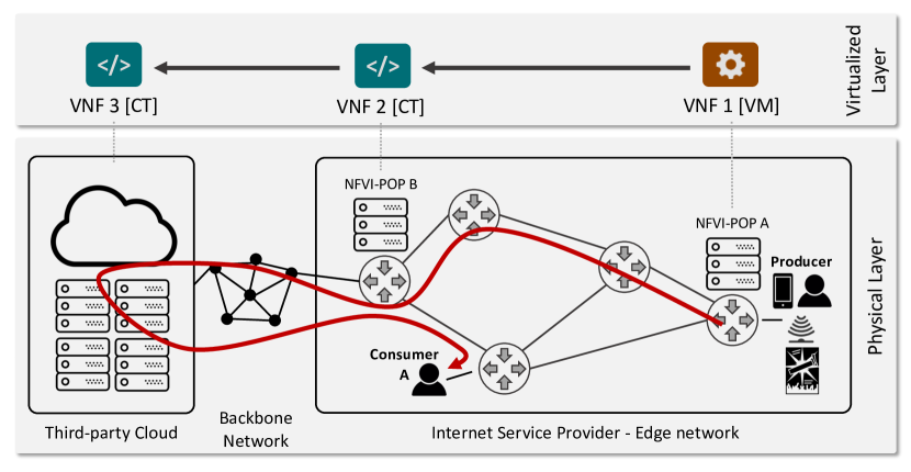
Figure 1: Example of hybrid SFC in an edge to cloud scenario

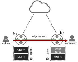
(a) Initial placement

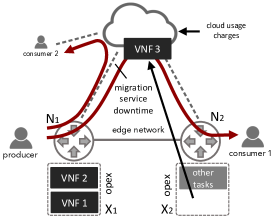
(b) Migration

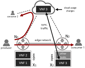
(c) Replication

Figure 2: Migration and replication examples after an initial placement

III System Model

III-A Reference Scenario

Fig. 1 illustrates the reference scenario. We assume that an ISP owns the network infrastructure close to the end users where it deploys small groups of servers for the NFV Infrastructure as Point-of-Presence (NFVI-POP) to run VNFs in an edge computing scenario. We also assume that the ISP uses the cloud as a third party to offload the VNFs when necessary. Let us now illustrate a hybrid SFC of three VNFs placed at different points in the network and cloud. Here, the ISP has to optimize the placement of VNFs while minimizing the operational costs of their deployment. In such scenarios, containerization technologies enhance NFV with a faster and more flexible way of provisioning the new services. Service providers can also flexibly place VNFs in either their own premises (i.e., at the network edge) or in third party cloud provider infrastructure. The decision on where to place VNFs is economy-driven. For instance, whereas placing VNFs in-network edge premises incurs energy and hardware maintenance costs, placing them on third party cloud providers adds additional charges that vary depending if they are deployed as VMs, usually charged per amount of used resources, or as containers, usually charged by duration of time. In both cases, the SLA violations need to be considered as penalty costs, which every ISP and cloud provider try to minimize.

III-B VNF Migrations and Replications

To illustrate the need for migrations or replications (be it for VM-VNFs and CT-VNFs), let us consider an example where three VNFs are chained and providing service to the traffic generated from one producer to one consumer. Let us consider a service provider edge network with two nodes, N1 and N2, with one server each $X_{1}$ and $X_{2}$, see Fig.2a. Server $X_{1}$ allocates VNFs 1 and 2, using all the resources in the server, while server $X_{2}$ allocates VNF 3, leaving the spare capacity to be used by other tasks. Now, let’s assume there is another consumer located in a different network (see Fig. 2b). In this case, since there are no free resources to serve the new service request, one option is to migrate VNF 3 to the cloud. This process is usually carried out by instantiating the new VNF and synchronizing the state before shutting shutting down the old one. However, there is a short service downtime caused by the control mechanisms for rerouting the traffic of the affected flows to the new location. This additional delay caused by the migration can affect the QoS and cause penalty costs to the service provider when the maximum delay specified in the SLA agreement is exceeded. On the other hand, there is also the possibility of replicating VNF 3 into the cloud without redirecting the original traffic, as shown in Fig. 2c. In this case, only the new traffic to the second consumer is redirected to the cloud to be processed by VNF 3. In this case, since we assume stateful VNFs, we need to consider the synchronization traffic between the original VNF and the replica. This example illustrates three basic costs to be considered when placing VNFs in the network or in the cloud: operational costs for maintaining servers in the edge network, additional charges when placing VNFs in the cloud and penalty costs when the service delay specified in the SLA agreement violated.

III-C Assumptions

For the sake of modeling and independently of placing VNFs in the edge or in the cloud, there are some assumptions to be considered here. First, when deploying VNFs over VMs in a model, one VNF instance maps 1:1 to a VM where some server resources are reserved to the VM to run independently of the processed traffic. This overhead is not considered when deploying VNFs as containers, since their performance is very close to bare metal. Regarding to delay, we define the end-to-end service delay, as the sum of propagation delay (time for the data to travel trough the fiber), processing delay (time for the VNF to process the data) and service interruption delays caused by migrations. Since before performing a migration, the new VNF in the new location has to be instantiated to then synchronize the states with the old VNF, the delay that affects to the service quality is the one related only to the short interruption of the active flows to commute and is independent from the VM or container size [34]. Although this delay is just temporal, we consider it as a key aspect to determine at some point in time whether a VM migration exceeds the maximum allowed service delay in the SLA agreement or not. In this sense, the service delay can be interpreted as a worst case delay. Since our model is multipath based, every service chain can use multiple paths, whereby each path can exhibit different delays due to different links traversed and the related VNFs. Regarding to the use of replications, it should be noted that in our model replications are used to address scalability during high load periods, and not for reliability purposes. We also consider the additional traffic generated by replicas to maintain their state synchronization independently if they run over VMs or containers. Unlike migrations, replicas do not induce extra service delay, since ongoing traffic demands are never interrupted during the replication process.

III-D Optimization Scenarios

Our approach to optimizations is carried out from the point of view of an ISP, or a network operator, who owns the physical server infrastructure in the edge network. So, given a certain network topology with servers located in every node, we assume that arbitrary nodes of that topology have links to a third party cloud. Then, in order to study the effect of migrations and replications have in the network and on the operational costs, we need to define two placement steps: one considering low traffic and one considering high traffic in the network. In this way, with low traffic we use it as an initial placement of VNFs where no replications are allowed, and of course no migrations have been performed from any previous step, and with high traffic some of the VNFs need to be migrated or replicated in order to provide service to the new traffic demands. On the other hand, thanks to the flexibility that NFV provides, we consider that the ISP is able to place VNFs in a third party cloud service provider in case, for instance, the network or the servers usage needs to be alleviated. In this case, this will incur additional costs for the ISP to pay when deploying VMs or instantiating containers in the third-party cloud. From the ISP point of view, neither the utilization of cloud servers nor the utilization of links connecting to the cloud is relevant, but the costs of that usage.

TABLE I: Notation

Parameters	Meaning
$\mathbb{N}$	set of nodes: $\mathbb{N}=\{1,...,N\}$, $n\in\mathbb{N}$.
$\mathbb{X}$	set of servers: $\mathbb{X}=\{1,...,X\}$, $x\in\mathbb{X}$.
$\mathbb{L}$	set of links: $\mathbb{L}=\{1,...,L\}$, $\ell\in\mathbb{L}$.
$\mathbb{P}$	set of all admissible paths: $\mathbb{P}=\{1,...,P\}$, $p\in\mathbb{P}$.
$\mathbb{S}$	set of SFCs: $\mathbb{S}=\{1,...,S\}$, $s\in\mathbb{S}$.
$\mathbb{T}$	set of VNF types: $\mathbb{T}=\{1,...,T\}$, $t\in\mathbb{T}$..
$\mathbb{V}_{s}$	ordered set of VNFs, where $v\in\mathbb{V}_{s}$ is the $v$th VNF in set $\mathbb{V}_{s}$.
$\Lambda$	set of all traffic demands: $\Lambda=\{1,...,\Lambda\}$, $\lambda\in\Lambda$.
$\Lambda_{s}\subseteq\Lambda$	subset of traffic demands $\lambda\in\Lambda_{s}$ for SFC $s\in\mathbb{S}$.
$\mathbb{N}_{p}\subseteq\mathbb{N}$	subset of ordered nodes traversed by path $p\in\mathbb{P}$.
$\mathbb{X}_{n}\subseteq\mathbb{X}$	subset of servers attached to node $n\in\mathbb{N}$.
$\mathbb{X}_{p}\subseteq\mathbb{X}$	subset of ordered servers traversed by path $p\in\mathbb{P}$.
$\mathbb{X}_{E}\subseteq\mathbb{X}$	subset of servers located at the edge.
$\mathbb{X}_{C}\subseteq\mathbb{X}$	subset of servers located at the cloud.
$\mathbb{P}_{s}\subseteq\mathbb{P}$	subset of admissible paths $p\in\mathbb{P}_{s}$ for SFC $s\in\mathbb{S}$.
$T_{p}^{\ell},T_{p}^{n,m}$	binary, 1 if path $p\in\mathbb{P}$ traverses the link $\ell\in\mathbb{L}$ and 1 if path $p\in\mathbb{P}$ connects node $n\in\mathbb{N}$ and $m\in\mathbb{N}$ as source and destination path nodes, respectively.
$\Gamma_{t(v)}^{\mathrm{pro}},\Gamma_{t(v)}^{\mathrm{syn}}$	floats, load ratio of a VNF of type $t\in V_{t}$ and traffic ratio for synchronization traffic between two VNFs of type $t\in V_{t}$, respectively.
$\Theta_{t(v)}^{s}$	integer, VM overhead for VNF $v\in\mathbb{V}_{s}$ of type $t\in V_{t}$.
$R_{t(v)}$	binary, 1 if VNF $v\in\mathbb{V}_{s}$ of type $t\in\mathbb{T}$ can be replicated.
$C_{x}^{\mathrm{max}},C_{\ell}^{\mathrm{max}}$	integers, maximum capacity of link $\ell\in\mathbb{L}$, maximum capacity of server $x\in\mathbb{X}$, respectively.
$C_{x,t(v)}^{\mathrm{pro\_q,max}}$	integer, maximum processing capacity that can be assigned by a server $x$ to a VNF of type $t$
$D_{\ell},D^{\mathrm{net}}$	floats, propagation delay of link $\ell\in\mathbb{L}$ and propagation delay that any demand can have in the network, respectively.
$D_{s}^{\mathrm{max}},\hat{D}_{s}^{\mathrm{{max}}}$	floats, maximum allowed delay for a SFC $s\in\mathbb{S}$ and maximum delay a SFC can have, respectively.
$D_{t(v)}^{\mathrm{pro,max}}$	floats, maximum allowed processing delay for a VNF of type $t$.
$D_{t(v)}^{\mathrm{pro\_q}},D_{t(v)}^{\mathrm{pro\_x}}$	floats, delay of a VNF $v$ of type $t$ due to queues and processing, respectively.
$D^{\mathrm{dwt}}$	float, service downtime duration caused by a migration.
Variables	Meaning
$z_{p}^{s}$	binary, 1 if SFC $s$ is using path $p\in\mathbb{P}_{s}$.
$z_{p}^{\lambda,s}$	binary, 1 if traffic demand $\lambda$ from SFC $s$ is using path $p\in\mathbb{P}_{s}$.
$f_{x}$	binary, 1 if server $x$ is used to place at least one function, 0 otherwise.
$f_{x}^{v,s}$	binary, 1 if VNF $v\in\mathbb{V}_{s}$ from SFC $s$ is allocated at server $x\in\mathbb{X}$, 0 otherwise.
$f_{x,\lambda}^{v,s}$	binary, 1 if VNF $v\in\mathbb{V}_{s}$ from SFC $s$ is being used at server $x\in\mathbb{X}$ by traffic demand $\lambda$, 0 otherwise.
$h_{p}^{v,s}$	binary, 1 if VNF $v\in\mathbb{V}_{s}$ from SFC $s$ is using path $p\in\mathbb{P}$ for state synchronization, 0 otherwise.
$d_{p}^{\lambda,s}$	positive float, end-to-end delay perceived by a traffic demand $\lambda$ using path $p$.
$q_{p}^{\lambda,s}$	positive float, penalty cost due to a traffic demand $\lambda\in\Lambda_{s}$ from SFC $s\in\mathbb{S}$ using path $p\in\mathbb{P}_{s}$.
$u_{\ell}$, $u_{x}$	positive floats, utilizations of a link $\ell\in\mathbb{L}$ and server $x\in\mathbb{X}$, respectively.

IV Problem Formulation

We model the network as $\mathbb{G}=(\mathbb{N}\cup\mathbb{X},\mathbb{L})$ where $\mathbb{N}=\{1,...,N\}$ is a set of nodes, $\mathbb{X}=\{1,...,X\}$ is a set of servers and $\mathbb{L}=\{1,...,L\}$ is a set of directed links. Specifically, $\mathbb{X}_{n}$ is a subset of servers $x\in\mathbb{X}$ attached to node $n\in\mathbb{N}$. We denote the set of all SFCs as $\mathbb{S}=\{1,...,S\}$, where a specific SFC $s\in\mathbb{S}$ is an ordered set of VNFs $\mathbb{V}_{s}=\{1,...,V_{s}\}$, each VNF being of type $t$, $t\in\mathbb{T}$, $\mathbb{T}=\{1,...,T\}$, where $v\in\mathbb{V}_{s}$ is the $v$^th VNF in set $V_{s}$. Table I summarizes the notations. It should be noted that the model is written such that it can be efficiently used in optimization solvers. For instance, the big M method is avoided when possible or its value is minimized in order to avoid numerical issues with the solver.

IV-A Objective Function

We define the joint optimization problem as the minimization of the sum of three different monetary costs: (i) costs of maintaining the servers, (ii) charges applied when placing VNFs in third party clouds and (iii) penalty costs incurred when violating SLA agreements due to the maximum service delay is exceed, i.e.,

$$\text{\emph{minimize:}}\quad\sum_{x\in\mathbb{X}_{E}}k_{x}^{E}+\sum_{x\in\mathbb{X}_{C}}k_{x}^{C}+\sum_{s\in\mathbb{S}}\sum_{\lambda\in\Lambda_{s}}\sum_{p\in\mathbb{P}_{s}}q_{p}^{\lambda,s}$$ (1)

, where the $k_{x}^{E}$ is the operational cost of a server $x$ at the edge network, $k_{x}^{C}$ are the charges of allocating VNFs into a server $x$ of a third party cloud provider and $q_{p}^{\lambda,s}$ is the penalty costs applied when the maximum end-to-end delay of a SFC $s\in\mathbb{S}$ has been exceed for traffic demand $\lambda\in\Lambda_{s}$ using path $p\in\mathbb{P}_{s}$. We next specify each cost individually.

IV-A1 Edge servers OPEX

To calculate the operational cost of each server $k_{x}^{E}$ at the edge, we consider the following linear function:

$$\forall x\in\mathbb{X}_{E}:k_{x}^{E}=f_{x}\cdot E_{i}+\alpha_{u}\cdot u_{x}+K_{x}$$ (2)

, where the variable $f_{x}$ determines if a server $x$ is used or not, $E_{i}$ is the energy consumption when the server is running idle, $\alpha_{u}$ determines the costs in relation to the server utilization $u_{x}$ and $K_{x}$ are the extra maintenance costs of a server independently of the energy consumption which we remove from our analysis since it has no effect on the optimization.

IV-A2 Cost of Third-Party Clouds

To determine the charges $k_{x}^{C}$ for all VNFs deployed in the cloud servers, we define:

$$\forall x\in\mathbb{X}_{C}:k_{x}^{C}=\sum_{s\in\mathbb{S}}\sum_{v\in\mathbb{V}_{s}}K_{t(v)}\cdot f_{x}^{v,s}$$ (3)

, where the parameter $K_{t(v)}$ specifies the charges of a specific VNF of type $t$, as long as the variable $f_{x}^{v,s}$ specifies that the VNF $v$ from SFC $s$ has been allocated in a server $x\in\mathbb{X}_{C}$ in the cloud. The parameter $K_{t(v)}$ will vary depending on whether the VNF runs over a VM or as a container.

IV-A3 Penalty costs

If a certain traffic demand $\lambda\in\Lambda_{s}$ from a SFC $s\in\mathbb{S}$ using a path $p\in\mathbb{P}_{s}$ exceeds the maximum service delay, then a penalty cost defined by the positive float variable $q_{p}^{\lambda,s}$ is applied, following:

$$\forall s\in\mathbb{S},\forall p\in\mathbb{P}_{s},\forall\lambda\in\Lambda_{s}:q_{p}^{\lambda,s}\geq\Bigg{(}\frac{d_{p}^{\lambda,s}}{D_{s}^{\mathrm{max}}}-1\Bigg{)}\rho_{s}\cdot z_{p}^{\lambda,s}$$ (4a)

$$\forall s\in\mathbb{S}:D_{s}^{\mathrm{max}}=\sum_{v\in\mathbb{V}_{s}}D_{t(v)}^{\mathrm{pro,max}}+D^{\mathrm{net}}$$ (4b)

$$\forall s\in\mathbb{S}:\rho_{s}=\rho\sum_{v\in\mathbb{V}_{s}}K_{t(v)}$$ (4c)

, where $d_{p}^{\lambda,s}$ is the delay variable associated to a specific traffic demand $\lambda$ using path $p$ (later explained in detail in Section IV-C5), $D_{s}^{\mathrm{max}}$ is the maximum allowed end-to-end delay for a specific SFC $s$, $\rho_{s}$ is the monetary penalty cost to be paid for that service if $d_{p}^{\lambda,s}$ is longer than $D_{s}^{\mathrm{max}}$ and $z_{p}^{\lambda,s}$ is the variable that determines whether the traffic demand $\lambda$ from the SFC $s$ is using path $p$ or not. $D_{s}^{\mathrm{max}}$ is calculated considering the maximum allowed processing delay $D_{t(v)}^{\mathrm{pro,max}}$ for every VNF in the chain plus the maximum propagation delay that a traffic demand can experience in the network $D^{\mathrm{net}}$. The monetary penalty costs $\rho_{s}$ is calculated as a percentage $\rho$ of the selling price for that SFC $s$, which is determined by the sum of all selling prices for every VNF in the chain. As selling prices for every VNF, we use the same values $K_{t(v)}$ as the ones used for the cloud charges. Due to the product of $d_{p}^{\lambda,s}$ and $z_{p}^{\lambda,s}$, we use the following linearization equations:

$$\forall s\in\mathbb{S},\forall p\in\mathbb{P}_{s},\forall\lambda\in\Lambda_{s}:y_{p}^{\lambda,s} \leq d_{p}^{\lambda,s}$$ (5a)

$$y_{p}^{\lambda,s} \leq\hat{D}_{s}^{\mathrm{{max}}}\cdot z_{p}^{\lambda,s}$$ (5b)

$$y_{p}^{\lambda,s} \geq\hat{D}_{s}^{\mathrm{{max}}}(z_{p}^{\lambda,s}-1)+d_{p}^{\lambda,s}$$ (5c)

, where $y_{p}^{\lambda,s}$ has value $d_{p}^{\lambda,s}$ when $z_{p}^{\lambda,s}$ is 1, 0 otherwise, and $\hat{D}_{s}^{\mathrm{{max}}}$ is the worst possible case of service delay that a service can have considering all service downtimes. So, $\hat{D}_{s}^{\mathrm{{max}}}$ is:

$$\hat{D}_{s}^{\mathrm{{max}}}=D_{s}^{\mathrm{max}}+|\mathbb{V}_{s}|\cdot D^{\mathrm{dwt}}$$ (6)

, where $|\mathbb{V}_{s}|$ is the total number of VNFs in the SFC and $D^{\mathrm{dwt}}$ is the service downtime duration caused by a single migration.

IV-B General Constraints

The general constraints are related to the traffic routing, the VNF placement and the mapping between VNFs and paths.

IV-B1 Routing

For a given network, the input set $p\in\mathbb{P}_{s}$ is the set of all pre-calculated paths for SFC $s$. The binary variable $z_{p}^{\lambda,s}=1$ indicates, that a traffic demand $\lambda\in\Lambda_{s}$ of the SFC $s$ is using path $p\in\mathbb{P}_{s}$. The first routing constraint specifies that each traffic demand $\lambda\in\Lambda_{s}$ from SFC $s\in\mathbb{S}$ has to use only one path $p\in\mathbb{P}_{s}$, i.e.:

$$\forall s\in\mathbb{S},\forall\lambda\in\Lambda_{s}:\sum_{p\in\mathbb{P}_{s}}z_{p}^{\lambda,s}=1$$ (7)

Then, the next constraint takes the activated paths from the variable $z_{p}^{\lambda,s}$ and activates the path for a certain SFC $s$:

$$\forall s\in\mathbb{S},\forall p\in\mathbb{P}_{s},\forall\lambda\in\Lambda_{s}:z_{p}^{\lambda,s}\leq z_{p}^{s}\leq\sum_{\lambda^{\prime}\in\Lambda_{s}}z_{p}^{\lambda^{\prime},s}$$ (8)

This forces $z_{p}^{s}$ to be 1 when at least one traffic demand is using path $p$, whereas the right side forces to $z_{p}^{s}$ to be 0 when no traffic demand $\lambda$ is using path $p$.

IV-B2 VNF placement

VNF placement is modeled using the binary variable $f_{x,\lambda}^{v,s}$, which has only value 1, if VNF $v$ from SFC $s$ is allocated at server $x\in\mathbb{X}$ and used by traffic demand $\lambda\in\Lambda_{s}$. Similarly to (7), the next constraint defines that each traffic demand $\lambda\in\Lambda_{s}$ from SFC $s\in\mathbb{S}$ has to traverse every VNF $v\in\mathbb{V}_{s}$ in only one server $x\in\mathbb{X}$:

$$\forall s\in\mathbb{S},\forall v\in\mathbb{V}_{s},\forall\lambda\in\Lambda_{s}:\sum_{x\in\mathbb{X}}f_{x,\lambda}^{v,s}=1$$ (9)

Then, similarly to (8), the next constraint takes the activated VNFs for each traffic demand from the variable $f_{x,\lambda}^{v,s}$ and activates the VNF for a certain SFC $s$ as follows:

$$\forall s\in\mathbb{S},\forall v\in\mathbb{V}_{s},\forall x\in\mathbb{X},\forall\lambda\in\Lambda_{s}:f_{x,\lambda}^{v,s}\leq f_{x}^{v,s}\leq\!\!\!\!\sum_{\lambda^{\prime}\in\Lambda_{s}}f_{x,\lambda^{\prime}}^{v,s}$$ (10)

, where the left side forces to $f_{x}^{v,s}$ to be 1 when at least one traffic demand $\lambda\in\Lambda_{s}$ is using VNF $v\in\mathbb{V}_{s}$ at server $x\in\mathbb{X}$ and the right side forces to $f_{x}^{v,s}$ to be 0 when no traffic demand is using that specific VNF $v$ on server $x$. Likewise, we determine if a server is being used or not by constraining the variable $f_{x}$ as:

$$\forall x\in\mathbb{X}:\frac{1}{|\mathbb{S}||\mathbb{V}_{s}|}\sum_{s\in\mathbb{S}}\sum_{v\in\mathbb{V}_{s}}f_{x}^{v,s}\leq f_{x}\leq\sum_{s\in\mathbb{S}}\sum_{v\in\mathbb{V}_{s}}f_{x}^{v,s}\text{ ,}$$ (11)

where $f_{x}$ is 1 if at least one VNF from any SFC is allocated at server $x\in\mathbb{X}$, 0 otherwise.

IV-B3 Mapping VNFs to paths

The next equation maps the activated VNF to the activated paths defined in the previous constraints. The first one defines how many times a VNF can be replicated:

$$\forall s\in\mathbb{S},\forall v\in\mathbb{V}_{s}:\sum_{x\in\mathbb{X}}f_{x}^{v,s}\leq R_{t(v)}\sum_{p\in\mathbb{P}_{s}}z_{p}^{s}+1-R_{t(v)}$$ (12)

, where $R_{t(v)}$ specifies if a certain VNF $v$ of type $t$ is replicable. When $R_{t(v)}$ is 0, the total number of activated VNFs $v\in\mathbb{V}_{s}$ from SFC $s\in\mathbb{S}$ is $\sum_{x\in\mathbb{X}}f_{x}^{v,s}\leq 1$. In case the VNF is replicable, then the maximum number of replicas is limited by the total number of activated paths $\sum_{p\in\mathbb{P}_{s}}z_{p}^{s}$ for that specific SFC $s$. The next constraint activates the VNFs on the activated paths:

$$\forall s\in\mathbb{S},\forall p\in\mathbb{P}_{s},\forall\lambda\in\Lambda_{s},\forall v\in\mathbb{V}_{s}:z_{p}^{\lambda,s}\leq\sum_{x\in\mathbb{X}_{p}}f_{x,\lambda}^{v,s}$$ (13)

If the variable $z_{p}^{\lambda,s}$ is activated, then every VNF $v\in\mathbb{V}_{s}$ from SFC $s\in\mathbb{S}$ has to be activated in some server $x\in\mathbb{X}_{p}$ from the path $p\in\mathbb{P}$ for a specific traffic demand $\lambda$. When $z_{p}^{\lambda,s}$ is deactivated, then no VNFs can be placed for that specific traffic demand. The last general constraint controls that all VNFs $V_{s}$ from a specific SFC $s$ are traversed by every traffic demand $\lambda\in\Lambda_{s}$ in the given order, i.e.:

$$\forall s\in\mathbb{S},\forall\lambda\in\Lambda_{s},\forall p\in\mathbb{P}_{s},\forall v\in\mathbb{V}_{s},\forall n\in\mathbb{N}_{p},\forall m\in\mathbb{N}_{p}:\\ \Bigg{(}\sum_{m=1}^{n}\sum_{y\in\mathbb{X}_{m}}\!\!f_{y,\lambda}^{(v-1),s}\Bigg{)}\!-\!\!\!\sum_{x\in\mathbb{X}_{n}}\!\!f_{x,\lambda}^{v,s}\geq z_{p}^{\lambda,s}\!-1\text{ for }1<v\leq|\mathbb{V}_{s}|$$ (14)

, where the variable $z_{p}^{\lambda,s}$ activates the ordering constraint side (left side) when is 1 and deactivates it, otherwise. Then, if path $p\in\mathbb{P}$ is activated, the ordering is checked for every traffic demand $\lambda\in\Lambda_{s}$ individually by using the variable $f_{x,\lambda}^{v,s}$. Hence, for every traffic demand $\lambda$ of SFC $s$, the $v$^th VNF is allocated at server $x\in\mathbb{X}_{n}$ only if the previous $(v-1)$^th VNF is allocated at any server $y\in\mathbb{X}_{m}$, where $m$ is the i^th node from 1 until $n$ traversed by path $p$. It should be noted, that the correct sequence of VNFs relies on the correct sequence of subset of servers, i.e. $x\in\mathbb{X}_{n}$. This assumes that the correct sequence of VNFs inside these subsets is organized by the local routing, which may be located at the node $n$ or at a local switch not modeled in detail.

IV-C Traffic and Performance Constraints

IV-C1 Initial placement parameter

Since the optimization process follows two different phases, after the initial placement we take the value of variables $f_{x}^{v,s}$ and convert them into the input parameters $F_{x}^{v,s}$ for the next next placement step, i.e.

$$\forall s\in\mathbb{S},\forall v\in\mathbb{V}_{s},\forall x\in\mathbb{X}:f_{x}^{v,s}\Rightarrow F_{x}^{v,s}$$ (15)

The parameter $F_{x}^{v,s}$ determines if a VNF $v$ of a service chain $s$ was placed on server $x$ during the initial placement.

IV-C2 Migration and replications

To identify a migration, the initial solution has to be mapped using (15). For evaluation and comparison reasons, the number of migrations $n_{mgr}$ can be calculated as follows:

$$n_{mgr}=\sum_{x\in\mathbb{X}}\sum_{s\in\mathbb{S}}\sum_{v\in\mathbb{V}_{s}}F_{x}^{v,s}(1-f_{x}^{v,s})$$ (16)

, where the variable $F_{x}^{v,s}$ specifies the initial placement, and $f_{x}^{v,s}$ indicates if the same VNF has been removed from the same server $x$. On the other hand, to count the number of replications for every VNF, we use:

$$n_{rep}=\sum_{s\in\mathbb{S}}\sum_{v\in\mathbb{V}_{s}}\big{[}(\sum_{x\in\mathbb{X}}f_{x}^{v,s})-1\big{]}\text{ ,}$$ (17)

where we do account for the original VNF.

IV-C3 Synchronization traffic

When performing replications of a specific VNF, the statefulness between the original and replicas has to be maintained in order to be reliable against VNF failures and avoiding the lost of information. For this reason, we consider that when a VNF is replicated, the generated synchronization traffic between replicas and the original has to be also considered. The amount of the state synchronization traffic depends on the state space and its time dynamic, where it is assumed, that each VNF has full knowledge on the state of all its instances used to implement the VNF $v\in\mathbb{V}_{s}$. Let us assume, that this amount is proportional to the total traffic offered to the SFC weighted by an synchronization ratio $\Gamma_{t(v)}^{\mathrm{syn}}$, which depends on the type of VNF $t$. In summary, the directional traffic from a VNF to its replica is given by $\Gamma_{t(v)}^{\mathrm{syn}}|\Lambda_{s}|$, and its routing should be optimized within the network.

In order to know if the same VNF $v\in\mathbb{V}_{s}$ from SFC $s$ is placed in two different servers $x\in\mathbb{X}$ and $y\in\mathbb{X}$, we define:

$$\forall s\in\mathbb{S},\forall v\in\mathbb{V}_{s},\forall x\in\mathbb{X},\forall y\in\mathbb{X},y\!\neq\!x:g_{x,y}^{v,s}=f_{x}^{v,s}f_{y}^{v,s}$$ (18)

, where the variable $g_{x,y}^{v,s}$ is 1 only when both variables $f_{x}^{v,s}$ and $f_{y}^{v,s}$ are also 1, and 0 otherwise. In this way, this variable is used to know if two different servers have the same VNF placed, which means that model is allocating one replica. We use the well-known linearization method when multiplying two binary variables. In case $g_{x,y}^{v,s}=1$, we need to carry the synchronization traffic from server $x$ to $y$, by selecting only one predefined path between them, i.e.:

$$\forall s\in\mathbb{S},\forall v\in\mathbb{V}_{s},\forall n,m\in\mathbb{N},n\neq m,\forall x\in\mathbb{X}_{n},\forall y\in\mathbb{X}_{m}:\\ g_{x,y}^{v,s}\leq\sum_{p\in\mathbb{P}}h_{p}^{v,s}\cdot T_{p}^{n,m}\leq 1\quad\text{ ,}$$ (19)

$$\forall s\in\mathbb{S},\forall v\in\mathbb{V}_{s},\forall n,m\in\mathbb{N},n\neq m:\\ \sum_{p\in\mathbb{P}}h_{p}^{v,s}\cdot T_{p}^{n,m}\leq\sum_{x\in\mathbb{X}_{n}}\sum_{y\in\mathbb{X}_{m}}g_{x,y}^{v,s}\quad\text{ ,}$$ (20)

, where the constant $T_{p}^{n,m}=1$ indicates, that the path $p\in\mathbb{P}$ exists which connects servers $x\in\mathbb{X}_{n}$ and $y\in X_{m}$ using the shortest path between nodes $n$ and $m$. The right term of (19) guarantees that only one path $p\in\mathbb{P}$ is selected by variable $h_{p}^{v,s}$. Moreover, (20) guarantees that this path is only used if at least one $g_{x,y}^{v,s}$ is 1. Note that $h_{p}^{v,s}$ is a binary variable used for every VNF $v$ of SFC $s$.

IV-C4 Link and server utilization

The utilization of a link is calculated as follows:

$$\forall\ell\in\mathbb{L}:u_{\ell}=\frac{1}{C_{\ell}^{\mathrm{max}}}\sum_{s\in\mathbb{S}}\sum_{p\in\mathbb{P}_{s}}\sum_{\lambda\in\Lambda_{s}}\lambda\cdot T_{p}^{\ell}\cdot z_{p}^{\lambda,s}+\\ \frac{1}{C_{\ell}^{\mathrm{max}}}\sum_{p\in\mathbb{P}}T_{p}^{\ell}\sum_{s\in\mathbb{S}}\sum_{v\in\mathbb{V}_{s}}\Gamma_{t(v)}^{\mathrm{syn}}\cdot|\Lambda_{s}|\cdot h_{p}^{v,s}\leq 1\text{ ,}$$ (21)

where $\lambda\cdot T_{p}^{\ell}$ adds the traffic demands from SFC $s\in\mathbb{S}$ when a path $p\in\mathbb{P}_{s}$ traverses the link $\ell\in\mathbb{L}$. Then, the variable $z_{p}^{\lambda,s}$ specifies if the traffic demand $\lambda$ from SFC $s$ is using path $p$. The second term is the sum of the extra traffic generated due to the state synchronization between VNFs $v\in\mathbb{V}_{s}$ from SFC $s$, which is proportional to its total traffic $|\Lambda_{s}|$ multiplied by the synchronization traffic ratio $\Gamma_{t(v)}^{\mathrm{syn}}$ of the VNF of type $t$. This traffic is only added, if the variable $h_{p}^{v,s}$ is 1, which indicates that path $p\in\mathbb{P}$ is used for synchronization by a VNF $v$ from SFC $s$, and the link $\ell\in\mathbb{L}$ belongs to this path. Both summation terms are divided by the maximum link capacity $C_{\ell}^{\mathrm{max}}$ to restrict the utilization.

The processing load of a server is derived as

$$\gamma_{x}=\sum_{s\in\mathbb{S}}\sum_{v\in\mathbb{V}_{s}}\Big{(}\Gamma_{t(v)}^{\mathrm{pro}}\sum_{\lambda\in\Lambda_{s}}\lambda\cdot f_{x,\lambda}^{v,s}+\Theta_{t(v)}^{s}\cdot f_{x}^{v,s}\Big{)}$$ (22)

, where the first term sums the traffic $\lambda\in\Lambda_{s}$ that is using the VNF $v\in\mathbb{V}_{s}$ from SFC $s\in\mathbb{S}$ at server $x\in\mathbb{X}$, which is determined by the variable $f_{x,\lambda}^{v,s}$, and multiplied by the processing load ratio $\Gamma_{t(v)}^{\mathrm{pro}}$ of the VNF of type $t$. The second term adds the overhead generated by the VM where the VNF is running and is only added, when the variable $f_{x}^{v,s}$ determines that this VNF is placed in server $x$. That term will be omitted when the VNF is deployed as CT-VNF, instead. Then, the utilization follows to be given by

$$\forall x\in\mathbb{X}:u_{x}=\frac{\gamma_{x}}{C_{x}^{\mathrm{max}}}\leq 1\text{ ,}$$ (23)

where $C_{x}^{\mathrm{max}}$ is the maximum processing capacity.

IV-C5 Service delay

Since every service has a maximum allowed delay $D_{s}^{\mathrm{max}}$ specified in the SLA agreement, in case of exceeding it, some penalty costs are applied. In our model, and for simplicity, we take into account the propagation delay due to the traversed links, the processing delay that every VNF requires in the servers and, where applicable, the downtime delays caused by the interruption of the service during the migrations of VNFs.

Processing delay: The processing delay $d_{x,v,s}^{\mathrm{pro}}$ of a VNF $v$ in a server $x$ depends, on the one side, on the amount of traffic being processed by a specific VNF, described by $d_{x,v,s}^{\mathrm{pro\_q}}$, and on $d_{x,v,s}^{\mathrm{pro\_x}}$, which is related to the VNF type and the total server load $u_{x}$, given as

$$\forall s\in\mathbb{S},\forall v\in\mathbb{V}_{s},\forall x\in\mathbb{X}_{p}:d_{x,v,s}^{\mathrm{pro}}=d_{x,v,s}^{\mathrm{pro\_q}}+d_{x,v,s}^{\mathrm{pro\_x}}$$ (24a)

$$d_{x,v,s}^{\mathrm{pro\_q}}=D_{t(v)}^{\mathrm{pro\_q}}\frac{\Gamma_{t(v)}^{\mathrm{pro}}\cdot\sum_{\lambda\in\Lambda_{s}}f_{x,\lambda}^{v,s}\cdot\lambda}{C_{x,t(v)}^{\mathrm{pro\_q,max}}}$$ (24b)

$$d_{x,v,s}^{\mathrm{pro\_x}}=D_{t(v)}^{\mathrm{pro\_x,min}}\cdot f_{x}^{v,s}+D_{t(v)}^{\mathrm{pro\_x}}\cdot u_{x}$$ (24c)

In (24b), the numerator of $d_{x,v,s}^{\mathrm{pro\_q}}$ determines the total processing load assigned to the VNF of type $t$, which is controlled by the variables $f_{x,\lambda}^{v,s}$. Thus, if the assigned processing load is equal to $C_{x,t(v)}^{\mathrm{pro\_q,max}}$, the VNF adds the processing delay $D_{t(v)}^{\mathrm{pro\_q}}$. The second delay term, given in (24c), adds the load independent minimum delay associated to the usage of a type of this VNF, and a delay part which increases with the server utilization. As a consequence the processing delay $d_{x,v,s}^{\mathrm{pro}}(\vec{\lambda})$ depends on the server $x$, the used VNF type and linearly increases with increasing traffic. Furthermore, the dependency on all traffic demands is denoted by the vector $\vec{\lambda}$, which is omitted for simplicity in (24).

Downtime duration: If a VNF $v$ of SFC $s$ has to be migrated, we assume an interruption of the service with duration $D^{\mathrm{dwt}}$. Thus, the total service downtime will consider the migration of all VNFs in that SFC which yields a constraint as follows:

$$\forall s\in\mathbb{S}:d_{s}^{\mathrm{dwt}}=D^{\mathrm{dwt}}\sum_{x\in\mathbb{X}}\sum_{v\in\mathbb{V}_{s}}F_{x}^{v,s}(1-f_{x}^{v,s})$$ (25)

, where the parameter $F_{x}^{v,s}$ determines if a VNF $v$ was placed on server $x$ during the initial placement. Thus, if a VNF migrates to another server $y\neq x$, the variable $f_{x}^{v,s}$ is equal to zero and the service downtime $D^{\mathrm{dwt}}$ has to be taken into account.

Total delay: Because the model allows that different traffic demands per service can be assigned to different paths, we define individual end-to-end delay $\hat{d}_{p}^{\lambda,s}$ for every traffic demand, as follows:

$$\forall s\in\mathbb{S},\forall\lambda\in\Lambda_{s},\forall p\in\mathbb{P}_{s}:\\ \hat{d}_{p}^{\lambda,s}=\sum_{\ell\in\mathbb{L}}D_{\ell}\cdot T_{p}^{\ell}+\sum_{x\in\mathbb{X}_{p}}\sum_{v\in\mathbb{V}_{s}}d_{x,v,s}^{\mathrm{pro}}(\vec{\lambda})\cdot f_{x,\lambda}^{v,s}+d_{s}^{\mathrm{dwt}}$$ (26)

The first term is the propagation delay, where $D_{\ell}$ is the delay of the link $\ell$, and $T_{p}^{\ell}$ specifies if the link $\ell$ is traverses by path $p\in\mathbb{P}_{s}$. The second term adds the processing delays caused by all VNFs from the SFC placed on the servers $x\in\mathbb{X}_{p}$, in which the variable $f_{x,\lambda}^{v,s}$ has to ensure that the demand $\lambda$ is processed at an specific server $x$. Finally, the third term is the total downtime duration due to the migrations of that service chain. It should be noted that the second term of (26) includes a nonlinear relation between the binary variable $f^{v,s}_{x,\lambda}$ and the delay variable $d_{x,v,s}^{\mathrm{pro}}$, which also depends on all decision variables $f^{v{{}^{\prime}},s{{}^{\prime}}}_{x,\lambda{{}^{\prime}}}$. To solve that, we introduce a new delay variable $d_{x,\lambda}^{v,s}$, which is bounded as follows:

$$d_{x,v,s}^{\mathrm{pro}}-D_{t(v)}^{\mathrm{pro,max}}(1-f_{x,\lambda}^{v,s})\leq d_{x,\lambda}^{v,s}\leq D_{t(v)}^{\mathrm{pro,max}}\cdot f_{x,\lambda}^{v,s}$$ (27)

If the VNF is selected at server $x$ by $f_{x,\lambda}^{v,s}=1$, the variable is lower bounded by the exact delay $d_{x,v,s}^{\mathrm{pro}}$ and upper bounded by the maximum VNF delay $D_{t(v)}^{\mathrm{pro,max}}$. Since $d_{x,v,s}^{\mathrm{pro}}\leq d_{x,\lambda}^{v,s}\leq D_{t(v)}^{\mathrm{pro,max}}$, the specific delay of a VNF can be restricted. If the VNF is not selected, i.e., $f_{x,\lambda}^{v,s}=0$, the variable has value $d_{x,\lambda}^{v,s}=0$, since the constant $D_{t(v)}^{\mathrm{pro,max}}$ makes the left size of (27) to be negative. Hence, the end-to-end delay is mapped to an upper and lower bounded variable $d_{p}^{\lambda,s}$ given as

$$\forall s\in\mathbb{S},\forall\lambda\in\Lambda_{s},\forall p\in\mathbb{P}_{s}:\\ d_{p}^{\lambda,s}=\sum_{\ell\in\mathbb{L}}D_{\ell}\cdot T_{p}^{\ell}+\sum_{x\in\mathbb{X}_{p}}\sum_{v\in\mathbb{V}_{s}}d_{x,\lambda}^{v,s}+d_{s}^{\mathrm{dwt}}\quad\text{,}$$ (28)

in which the bounding feature is used in the optimization scenarios described next.

IV-D Optimization Scenarios

According to Section III, we divide the placement into two different phases, one where the VNFs are placed in the network only considering low traffic and another one when some of these VNFs are migrated and/or replicated in order to serve the new traffic demands. For the initial placement, from the set of traffic demands $\Lambda_{s}$ of SFC $s\in\mathbb{S}$, only a subset of demands $\lambda\in\Lambda_{s}$ is selected, where each demand is randomly selected with probability $R$ to be an element of the reduced set $\Lambda_{s}^{\prime}$. If no demand is selected, the reduced set contains at least one demand randomly selected out of $\Lambda_{s}$. For both cases, initial placement and second placement, the constraints (7) - (14) and (21) - (28) apply. Only for the second placement, the constraints (15), (18) - (20) also apply.

V Online Heuristic Approaches

Since the model presented is a MILP optimization problem and these models are known to be NP-hard [35], in this section we propose a greedy algorithm to work as an online solution and, First-Fit and Random-Fit algorithms for comparison purposes.

V-A First-Fit and Random-Fit algorithms

Both First-Fit (FF) and Random-Fit (RF) algorithms pseudo code are described in Algorithm 1. While both approaches share most of the code, the variable alg (line 1) specifies whether the code has to run FF or RF. The process starts with a loop where every demand from every SFC is going to be considered (line 2). The first step is to then retrieve all the paths with enough link resources to assign traffic demand $\lambda$ and that also connect both source and destination nodes (line 3). These paths are saved into $\mathbb{P}_{s}^{\prime}$, from where one admissible path $p$, first one for FF or a random one for RF, is selected (line 4). In this point, we make sure here that in this path, there are enough server resources to allocate all the VNFs for SFC $s$ (line 5). From that path, we start selecting a server for every VNF $v$ from SFC $s$. First, we retrieve all servers with enough free capacity to allocate the VNF $v$ and to provide service to demand $\lambda$ (line 6), and then we choose the first available server in FF or a random one in RF (line 7). It is to be noted here, that to satisfy VNF ordering (see equation 14), the procedure chooseServer will return a valid server from before/after the previous/next VNF allocated. While for the FF case, we assure in line 4 that there will always be a server where to allocate the next VNF in the chain, in RF case we make sure here (line 7) that after the random server selected there is still place to allocate all the rest of the VNFs from the chain in next servers in the path, or we select another server instead. In line 8, we assign the demand and the VNF to the server (i.e. equations (9) and (10)). After all the VNFs have been placed, the next step is to route traffic demand $\lambda$ to path $p$ (line 9), to finally add the synchronization traffic for the service chain (line 10).

Algorithm 1 First-Fit and Random-Fit algorithms

1:procedure simplePlacement($alg$)

2:     for $s\in\mathbb{S}$, $\lambda\in\Lambda_{s}$ do

3:         $\mathbb{P}_{s}^{\prime}\leftarrow$ getAdmissiblePaths($s$, $\lambda$)

4:         $p\leftarrow$ choosePath($alg$, $\mathbb{P}_{s}^{\prime}$)

5:         for $v\in\mathbb{V}_{s}$ do

6:              $\mathbb{X}_{p}^{\prime}\leftarrow$ getAvailableServers($s$, $\lambda$, $v$, $p$)

7:              $x\leftarrow$ chooseServer($alg$, $\mathbb{X}_{p}^{\prime}$)

8:              addVNFToServer($s$, $v$, $\lambda$, $x$)          

9:         routeDemandToPath($s$, $p$, $\lambda$)

10:         addSynchronizationTraffic($s$)      

Algorithm 2 Greedy algorithm

1:procedure main

2:     for $s\in\mathbb{S}$, $\lambda\in\Lambda^{\prime}_{s}$ do

3:         allocateDemand($s$, $\lambda$) $\triangleright$ go to 23      

4:     for $s\in\mathbb{S}$ do

5:         for $\lambda\in\Lambda^{\prime\prime}_{s}$ do

6:              allocateDemand($s$, $\lambda$) $\triangleright$ go to 23          

7:         addSynchronizationTraffic($s$)      

8:     $b\leftarrow$ computeObjVal()

9:     findNewIncumbent($b$) $\triangleright$ go to 10

10:procedure findNewIncumbent($b$)

11:     for $s\in S^{\prime}$ do

12:         for $s\in S^{\prime}$ do

13:              for $\lambda\in\Lambda_{s}$ do

14:                  removeDemandFromVNFs($s$, $\lambda$)

15:                  removeDemandFromPath($s$, $\lambda$)

16:                  $b^{\prime}\leftarrow$ simplePlacement($RF$)

17:                  if $b^{\prime}<b$ then

18:                       $b\leftarrow b^{\prime}$

19:                       setNewIncumbent()

20:                  else

21:                       undoPlacement()                                 

22:              reAssignSyncTraffic($s$)               

23:procedure allocateDemand($s$, $\lambda$)

24:     $\mathbb{P}_{s}^{\prime}\leftarrow$ getAdmissiblePaths($s$, $\lambda$)

25:     for $p\in\mathbb{P}_{s}^{\prime}$ do

26:         $p\leftarrow$ choosePath($s$, $\lambda$, $\mathbb{P}_{s}^{\prime}$) $\triangleright$ go to 32

27:         for $v\in\mathbb{V}_{s}$ do

28:              $\mathbb{X}_{p}^{\prime}\leftarrow$ getAvailableServers($s$, $\lambda$, $p$, $v$)

29:              $x\leftarrow$ chooseServer($s$, $\lambda$, $p$, $v$, $\mathbb{X}_{p}^{\prime}$) $\triangleright$ go to 40

30:              addVNFToServer($v$ , $x$)          

31:         routeDemandToPath($s$, $p$, $\lambda$)      

32:procedure choosePath($s$, $\lambda$, $\mathbb{P}_{s}^{\prime}$)

33:     $p\leftarrow$ getUsedPathForDemandInitPlacement($s$, $\lambda$, $\mathbb{P}_{s}^{\prime}$)

34:     if $p$ then return $p$      

35:     $p\leftarrow$ getUsedPathInitialPlacement($s$, $\mathbb{P}_{s}^{\prime}$)

36:     if $p$ then return $p$      

37:     $p\leftarrow$ getUsedPathForSFC($s$, $\mathbb{P}_{s}^{\prime}$)

38:     if $p$ then return $p$      

39:     return getPathWithShortestDelay($s$, $\lambda$, $\mathbb{P}_{s}^{\prime}$)

40:procedure chooseServer($s$, $\lambda$, $p$, $v$, $\mathbb{X}_{p}^{\prime}$)

41:     $\mathbb{X}_{p}^{\prime}\leftarrow$ removeServersPreviousVNFs($\mathbb{X}_{p}^{\prime}$)

42:     $\mathbb{X}_{p}^{\prime}\leftarrow$ removeServersNextVNFs($\mathbb{X}_{p}^{\prime}$)

43:     $x\leftarrow$ getUsedServerDemandInitialPlace($s$, $v$, $\lambda$, $\mathbb{X}_{p}^{\prime}$)

44:     if x then return x      

45:     $c\leftarrow$ returnCloudServer($\mathbb{X}_{p}^{\prime}$)

46:     $x\leftarrow$ getUsedServerInitialPlacement($s$, $v$, $\mathbb{X}_{p}^{\prime}$)

47:     if indexOf($x$) < indexOf($c$) then return x      

48:     $x\leftarrow$ getUsedServerForSFC($s$, $v$, $\mathbb{X}_{p}^{\prime}$)

49:     if indexOf($x$) < indexOf($c$) then return x      

50:     return $\mathbb{X}_{p}^{\prime}$[0]

V-B Greedy algorithm

The greedy algorithm pseudo code is described in Algorithm 2. The main procedure starts first allocating all demands $\Lambda^{\prime}_{s}$ from all SFCs used during the initial placement (line 2) and then, continues with the rest of traffic demands $\Lambda^{\prime\prime}_{s}$ (line 5), where $\Lambda^{\prime\prime}_{s}=\Lambda_{s}\setminus\Lambda^{\prime}_{s}$. In this way, we assure there are no migrations of VNFs during the initial placement. In both cases, we are pointing out to the function defined in line 23 which allocate traffic demand in the network while traversing the required VNFs (explained later in detail). After the allocation of all demands is done, we add the synchronization traffic between the replicas (line 7). Once all the resources are allocated in the network, we go back to line 8 and save the current objective value. From this point, starting from line 11, we go over all SFCs and try to improve the current solution by randomly switching demands. To do that, for every traffic demand, we first remove it from the current VNFs assigned and from the network (line 14 and 15) and then perform a random fit placement (line 16) following Algorithm 1 using a random placement. If the new objective value $b^{\prime}$ is lower, the placement is set as incumbent, otherwise is undone (lines 17-21). After the reallocation of VNFs, the synchronization traffic is reassigned (line 22).

Going into detail on the allocation of demands VNFs (line 23), the procedure starts by retrieving all paths with enough free link resources in $\mathbb{P}_{s}^{\prime}$ (line 24). Then, we choose a path $p$ inside of a loop from all retrieved paths (line 26, details explained later). This is done to make sure in case a path cannot be used for allocating all VNFs, the algorithm tries with the next one. Once the path is selected, we start with the placement of all VNFs on the selected path. First, all the available servers for an specific VNF $v$ on path $p$ are retrieved in variable $\mathbb{X}_{p}^{\prime}$ (line 28), then we choose one server $x$ for that specific VNF in line 29 (this procedure explained later) and place the VNF (line 30). In case the VNF has been already placed by another demand of the same service, the demand is associated to that VNF, instead. Finally after all VNFs are placed, we route the demand over path (line 31).

When selecting a path for a specific traffic demand (line 32), we execute the following methods in this specific order: return the already used path for the same demand $\lambda$ during the initial placement (line 33), return any used path for SFC $s$ during the initial placement (line 35), return any used path for SFC $s$ (line 37) or return the path with shortest path delay (line 39). If one method does not return a path, then the next one is executed. On the other hand, when choosing a server for a specific VNF (line 40), we first remove servers in the path that have already allocated VNFs before/after the current VNF in order to satisfy with chain order equation (14) in lines 41 and 42. And then, we are first try to use a server already used for VNF $v$ and demand $\lambda$ during the initial placement (line 43). If none, then we first return the cloud server, if any in path $p$, into variable $c$ (line 45) and then we try to get any server already used during the initial placement for VNF $v$ into variable $x$ (line 46). If that server is located in a node of the path that comes before in the sequence order than the cloud node, then we use it (line 47), otherwise, we try to use any other already used server for that VNF also if it is before in the path than the cloud (lines 48 and 49). In case there is no cloud in the path, both previous conditions are always true. If none of the previous methods worked, then we just return the first available server (line 50). This procedure is done in order to minimize the number of migrations and replications that cause an increment of the monetary costs.

TABLE II: Parameters for VM and CT based VNFs

	$\Theta_{t(v)}^{s}$	$\Gamma_{t(v)}^{\mathrm{pro}}$	$\Gamma_{t(v)}^{\mathrm{syn}}$	$C_{x,t(v)}^{\mathrm{pro\_q,max}}$	$D_{t(v)}^{\mathrm{pro\_q}}$	$D_{t(v)}^{\mathrm{pro\_x}}$	$D_{t(v)}^{\mathrm{pro\_x,min}}$	$D_{t(v)}^{\mathrm{pro,max}}$	$K_{t(v)}$ (cloud)
VM	7	1.2	0.1	72	3 ms	5 ms	2 ms	10 ms	0.0069 $/h
CT	0								0.1199988 $/h

V-B1 Computational complexity

In terms of complexity from bottom to top, for the procedure chooseServer in line 40 considering $V_{L}$ as the length of the longest SFC, it is in the order of $O(cs)=O(V_{L}\cdot|\mathbb{X}|)$. The procedure choosePath in line 32 is in the order of $O(cp)=O(P_{S})$ where $P_{S}$ is the number of paths per SFC. The procedure allocateDemand in line 23 is calculated based on $O(cs)$ and $O(cp)$, and is in the order of $O(ad)=O(P_{S}\cdot L_{P}[O(cp)+V_{L}\cdot O(cs)])$. The addSynchronizationTraffic procedure specified in line 7 is in the order of $O(st)=O(V_{L}\cdot|\mathbb{X}^{2}|\cdot|\mathbb{P}|)$. The findNewIncumbent procedure in line 9 is in the order of $O(fi)=O(|\Lambda|^{2})$ and the reAssignSynTraffic in line 22 is $O(rs)=V_{L}\cdot|\mathbb{X}^{2}|\cdot|\mathbb{P}|$. So, finally, the complexity of the entire algorithm is in the order of $O(|\Lambda|\cdot O(ad)\cdot O(st)+O(fi)\cdot O(rs))$.

VI Performance evaluation

We first evaluate a smaller size network using the MILP model (implemented using Gurobi Optimizer) and heuristics, and, then, we evaluate a larger network using heuristics only. The small size network analyzed has 7 nodes and 20 directed links with 500 units of capacity each (see Fig. 3a), located within a small city area, with 3 nodes nodes are connected to a distant cloud node (node c). The second, large network has 44 nodes and 140 directed links with 5000 units of capacity (see Fig. 3b) with 13 nodes connected to a cloud node. To calculate the propagation delays in real geographic locations, we used examples of Braunschweig (edge) and Frankfurt (cloud) in Germany for the small network. For the larger network, which is based of Palmetto network (South Carolina), we used the real locations whereas the cloud is located in North Virginia in the USA. In both cases, the location of the cloud is chosen based on the closest common locations that cloud providers offer. We now calculate the propagation delay by calculating the distance between nodes from their latitude and longitude using the Haversine method divided by 2/3 the speed of light. We thereby assume the links used to connect to the cloud are out of the ISP premises, have sufficient capacity for any demand, and therefore do not impact the analysis. In all cases, the propagation delay due to the distance to the cloud it will be taken into account. Every node in the small network has one server, while in the large network every node has 8 servers, in both cases with all servers with 1000 units of capacity. On the other hand, the cloud node has in both cases one server with a large capacity also to not interfere on the results. In the edge network, the costs due to the power consumption for every server specified in equation (2) have been calculated considering the power consumption of a Dell PowerEdge R410 Rack in Watts server specified in the spec sheet [36] multiplied by the average monetary costs of the electricity in USA is 0.139 $/kWh, so $E_{i}$ = 0.0184453 and $\alpha_{u}$ = 0.0095632. All other parameters are the same for both networks.

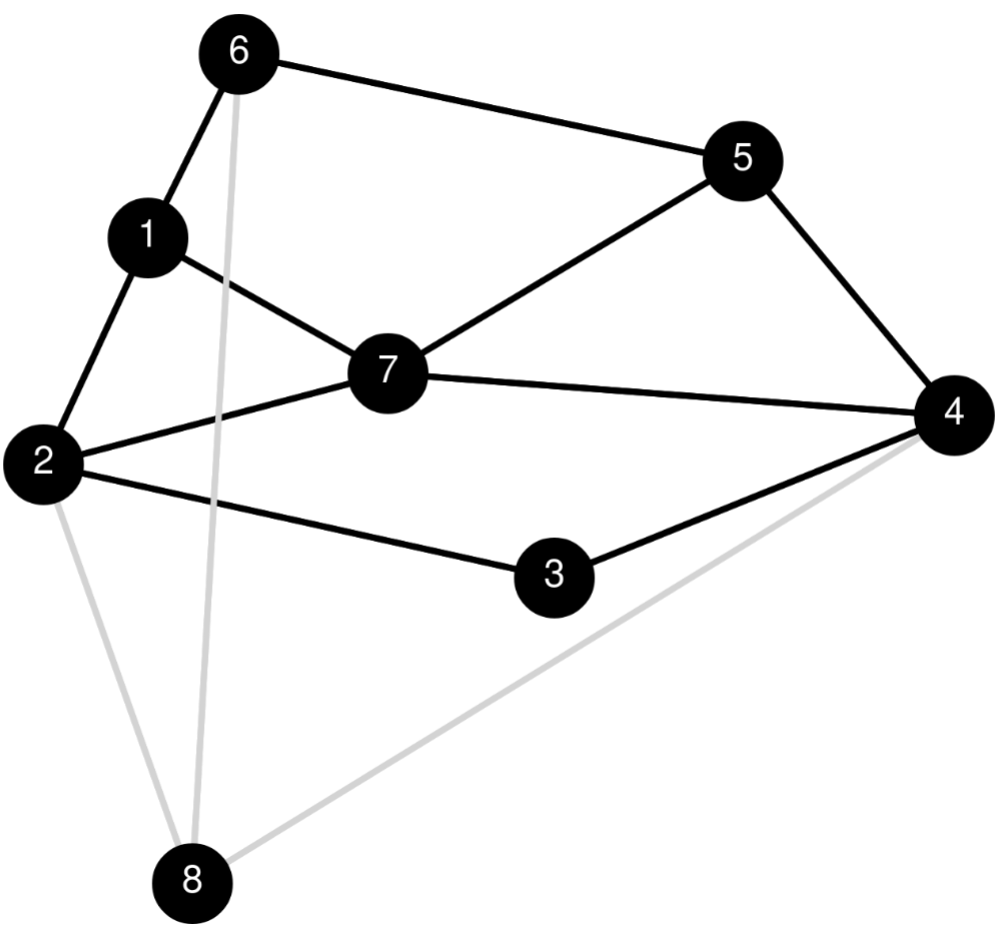
(a) 7 nodes network

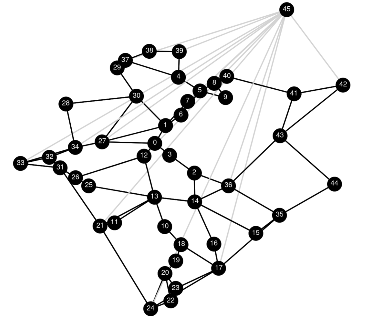
(b) 44 nodes network

Figure 3: Network topologies used for the performance evaluation.

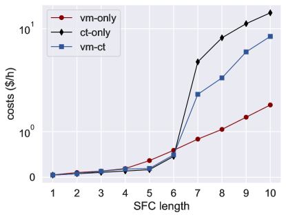
(a) Total costs

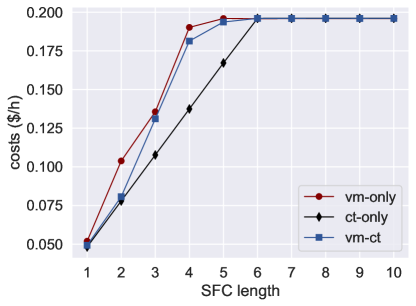
(b) OPEX costs

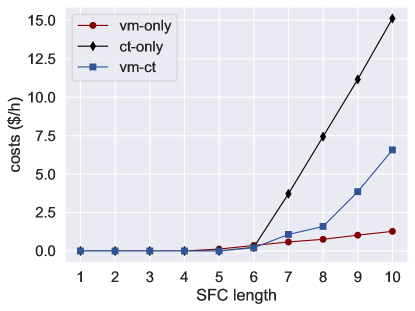
(c) Cloud charges

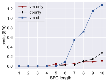
(d) Penalty costs

Figure 4: Comparison of total and individual costs from MILP model for different SFC lengths in network A.

For each source-destination pair of nodes, 3 paths are pre-computed that do not traverse the cloud node and 1 additional path that does. The path computation is carried out is this way to make sure the model has enough freedom to allocate all SFCs at the edge and at least there is one admissible path per SFC to allocate VNFs in the cloud. We assume that every source-destination pair of nodes instantiates independent SFCs and randomly generates between 1 and 3 traffic flows, each one with a bandwidth between [1, 20] units. Considering $\Lambda$ as the total set of traffic demands in the network, for the initial placement we only consider a subset $\Lambda^{\prime}$ generated by using a selection probability of $R=0.3$. In order to make a fair comparison between VMs and containers, we assume that the VNFs themselves have the same parameters irrespectively off the VM or container configurations; the only difference is the overhead introduced by VMs ($\Theta_{t(v)}^{s}$) and the charges applied when allocating VNFs in the cloud ($K_{t(v)}$). The overhead $\Theta_{t(v)}^{s}$ is calculated as  10% of the maximum processing capacity $C_{x,t(v)}^{\mathrm{pro\_q,max}}$ that a VNF can have [37]. Since $C_{x,t(v)}^{\mathrm{pro\_q,max}}$ is maximum possible processing capacity that a VNF can handle, it is calculated based on the worst case scenario, which is as the maximum number of traffic demands multiplied by the maximum possible bandwidth and by the traffic load ratio $\Gamma_{t(v)}^{\mathrm{pro}}$. The rest of the parameters can be found in Table II. Then, for every s-d combination (except the cloud node), one SFC is created to provision a service. The length of the SFCs varies from one to ten VNFs and we compare the cases where all VNFs in the SFCs are deployed only over VMs (vm-only), only over containers (ct-only), or hybrid, i.e., when both types are combined (vm-ct). For hybrid SFCs, the VNFs are randomly assigned either VMs or CTs, following a uniform distribution considering all possible combinations. Finally, the penalty parameter $\rho$ is computed as 10% of the selling price for an specific SFC (see [32] or [38]), which depends on the VNFs allocated to provide that specific service. So, to calculate the selling price for every SFC, we consider the same selling prices as for the charges of the cloud provider, so we use $K_{t(v)}$ values as well for every VNF deployed at the edge. In the proposed networks, for all SFCs the maximum propagation delay considered is $D^{\mathrm{net}}=5ms$ considering round trip time from both edge networks to the cloud. With this propagation delay, the maximum service downtime caused by migrations is expected to be $D^{\mathrm{dwt}}=27.5ms$ [34].

VI-A MILP model

VI-A1 Optimization Costs

Fig. 4a shows the total monetary cost (equation (1)) comparison for different SFC lengths in the small network (Fig. 3a) using the MILP model. As it can be seen, until SFC length 4, all three cases result in a comparable cost value, while between length 4 and 6, vm-only gets higher costs than the other two cases. This later case is interesting to show how the overhead introduced by VMs overload the edge servers earlier than the other two cases, incurring into higher costs. With length longer than 6, both ct-only and vm-ct get much higher costs than vm-only, being ct-only the worst case. This behavior can be explained by the fact that above length 6, the edge network is overloaded and the cloud needs to be used incurring into more charges due to container charges being higher than VMs. It is remarkable than the hybrid case gets relatively close values to the ct-only case. Looking into the costs individually, Fig. 4b, Fig. 4c and Fig. 4d show the OPEX costs, cloud charges and penalty costs. From the OPEX costs we confirm that in all cases the edge servers are full with SFC length 6 and above. Here we notice that while vm-only is the one incurring into more costs, vm-ct costs are not much lower and ct-only case is the one with lower costs until length 6. The opposite happens with cloud charges where ct-only is the worse case by far compared to the other two. If we take a look into the penalty costs results, we can see how the hybrid vm-ct has much higher above length 6 than the other two cases. This latter case is interesting because we observe how the model penalizes these costs which are compensated by highly reducing the cloud charges which the respective values have higher impact on the total costs. This effect on the penalty costs for the vm-ct case is correlated with the number of migrations (as shown later), which exceed the maximum allowed service delay.

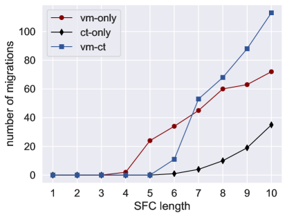
(a) Migrations

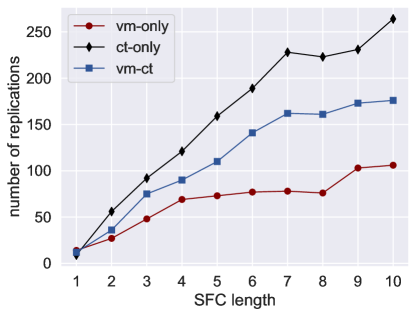
(b) Replications

Figure 5: Total number of migrations and replications for different SFC lengths

VI-A2 Migrations and Replications

In order to better understand the costs results, we show in Fig. 5a and Fig. 5b the number of VNF migrations and replications, respectively, which have a direct impact on the costs. We can see that the model starts earlier to perform migrations in the vm-only case, but with length 7 and above, the vm-ct case performs more migrations than any other case. While this behavior is interesting, it is hard to explain why this occurs. One possible explanation could be that these migrations occur within the edge network having a minimal impact on the penalty costs, as we can see in the previous Fig. 4d. On the other hand, for the number of replications, the vm-only performs less replications than the other two cases, being the vm-ct case an intermediate solution. This result is as expected since VMs introduce an overhead, so the model tries to minimize them.

VI-A3 Resource Utilization and Service Delay

Fig. 6a shows the average link utilization results for all links in the network except those connecting to the cloud. Here, we can see how the average network utilization for the vm-only is mostly lower than in the other two cases, being ct-only the one with higher average and vm-ct case an intermediate solution. This is due to the synchronization traffic between replicas that has to be added to the network load, and these results are consistent with the number of replicas shown previously in Fig. 5b. In all three cases, we can also see how above length 5, the average decreases due to the migration of VNFs to the cloud, which minimizes the traffic in the edge network. On the other side, the average server utilization, shown in Fig. 6b, confirms the OPEX costs results, showing how the edge network is overloaded when the length is above 6. It should be noted that even though the number of replicas is higher for ct-only, this does not affect to the average server utilization since there is no overhead introduced.

Fig. 6c shows the average end-to-end service delay between all SFCs deployed in the network. Here, vm-only increases linearly with the SFC length and is the one with comparably lower delay. While vm-ct has a similar average delay, above length 6, the value increases faster, being higher than ct-only case above length 9. This behavior is correlated to the number of migrations that can occur, due to the impact of service interruptions on the overall delay. While this tendency can be a concern, considering that in this case the edge network is completely overloaded and, therefore, requires heavy offloading to the cloud, the delays due to migrations are not a relevant in the cloud environments.

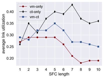
(a) Average link utilization

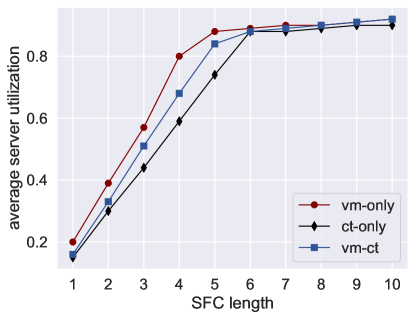
(b) Average server utilization

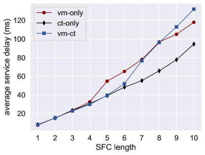
(c) Average service delay

Figure 6: Resource utilization and service delays for different SFC lengths

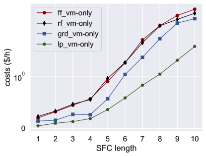
(a) Total costs with vm-only

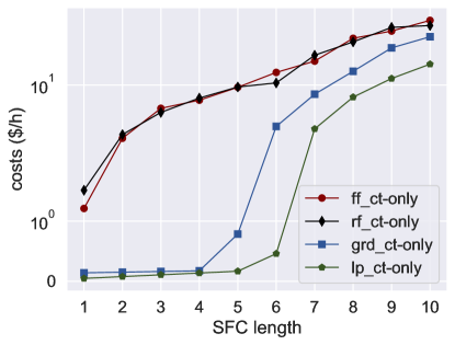
(b) Total costs with ct-only

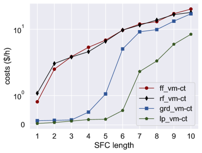
(c) Total costs with vm-ct

Figure 7: Comparison of algorithms for different SFC lengths in small scale network.

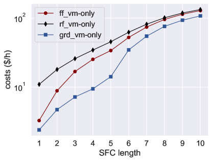
(a) Total costs with vm-only

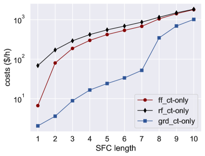
(b) Total costs with ct-only

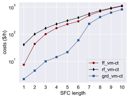
(c) Total costs with vm-ct

Figure 8: Comparison of algorithms for different SFC lengths in large scale network.

VI-B Heuristics

Here, we first compare the performance of the greedy algorithm compared to the optimal solution and to both first-fit and random-fit for the small scale network (Fig. 3a). Fig. 7a, Fig. 7b and Fig. 7c show the total monetary costs obtained using first-fit (ff), random-fit (rf), greedy (grd) and MILP (lp) for for the vm-only, ct-only and vm-ct cases, respectively. We can observe from all three cases that there is not much difference between first-fit and random-fit algorithms. The fact that random-fit behaves similar to first-fit can be due to the influence of the sequence order of VNFs have in the network, which is relatively small. Even with random placement, there is no much freedom of choice when placing VNFs, due to size. Thus, the available servers are restricted by the placement of the previous and next VNF of the chain in a specific path. In both cases, the fact that these algorithms do not take into account where the VNFs were placed during the initial placement, results in too many migrations and replications that increase the penalty costs and resource utilization, respectively. On the other hand, we can see how the greedy algorithm performs really close to the optimal solution when the SFC length is up to 4, when the servers at the edge are still not overloaded. For longer chains, the algorithm performs slightly worse due to the edge servers are overloaded and the cloud must be used, leading to a situation where the algorithm has less freedom for placements. In Fig. 8, we show the same costs for the large network (see Fig. 3b), with heuristics only. As in the case of smaller network, we can see how the greedy algorithm works better for ct-only than for the vm-only case.

VI-C Discussion and remarks

From the cost optimization point of view, we can see how the placement of VNFs on servers at the edge incurs lower costs when the ISP owns the server infrastructure as compared to the case of using a third party cloud provider. Specifically, the use of CT-VNF reduces the total costs even in hybrid scenarios with VM-VNF. In the situations when the use of the cloud is necessary, CT-VNF can result in excessive costs as compared to VMs only, but the combination of both in a hybrid SFC can alleviate these costs. We also showed how the preceding placement of VNFs in the network impacts the resulting the costs for the subsequent reallocations, since the number of migrations are going to affect the penalty costs, while the number of replications impact the resource usage. We also observe that when the edge network has enough server resources for allocation, greedy algorithm that performs close to the optimal solution (MILP). One relevant extension of the model would be to consider the sharing of VNFs of the same type between different SFCs, so it can be used for studying reliability [39]. Finally, while our model used generic VNF parameters, and the results may change with real-world parameters, the model can still provide some important clues on how the migration from VM to containers, and their hybrid combination with VMs can affect the cost models from the ISP’s point of view.

VII Conclusions

We studied a novel problem of optimal placement of hybrid SFCs, a combination of virtual machines and containers, from an Internet Service Provider (ISP) point of view, in a generic edge and cloud continuum. To this end, we proposed a Mixed-Integer Linear Programming model as well as a heuristic solution to solve the cost optimization problem that considers three objectives unique to the specific VM and container deployment in a carrier network: operational costs for maintaining servers in the edge, costs of placing VNFs in third-party cloud providers and penalty costs applied when SLA agreements are violated in terms of end-to-end delay. We also proposed 2-phases optimization process to analyze the effect on performance as a result of replications and migrations of VNFs. For larger networks, we developed a greedy algorithm that performs close to the optimal solution when there are enough free resources in the edge network. The results have shown that from the cost optimization point of view, the placement of VNFs on servers at the edge incurs lower costs when the ISP owns the server infrastructure compared to the case of using a third party cloud provider. As future work, we plan to extend the model for supporting shared VNFs and evaluate other kind scenarios where the objective if focused on the resource utilization.

References

- [1] ETSI, “Network Functions Virtualisation (NFV); Reliability; Report on Models and Features for End-to-End Reliability,” 2016.
- [2] Amazon, “AWS Lambda.” [Online]. Available: https://aws.amazon.com/lambda/
- [3] F. Alvarez, D. Breitgand, D. Griffin, P. Andriani, S. Rizou, N. Zioulis, F. Moscatelli, J. Serrano, M. Keltsch, P. Trakadas, T. K. Phan, A. Weit, U. Acar, O. Prieto, F. Iadanza, G. Carrozzo, H. Koumaras, D. Zarpalas, and D. Jimenez, “An Edge-to-Cloud Virtualized Multimedia Service Platform for 5G Networks,” IEEE Transactions on Broadcasting, vol. 65, no. 2, pp. 369–380, 2019.
- [4] M. M. Tajiki, S. Salsano, L. Chiaraviglio, M. Shojafar, and B. Akbari, “Joint Energy Efficient and QoS-aware Path Allocation and VNF Placement for Service Function Chaining,” IEEE Transactions on Network and Service Management, vol. PP, no. c, p. 1, 2017. [Online]. Available: http://arxiv.org/abs/1710.02611
- [5] L. Wang, Z. Lu, X. Wen, R. Knopp, and R. Gupta, “Joint Optimization of Service Function Chaining and Resource Allocation in Network Function Virtualization,” IEEE Access, vol. 4, pp. 8084–8094, 2016.
- [6] A. Basta, A. Blenk, K. Hoffmann, H. J. Morper, M. Hoffmann, and W. Kellerer, “Towards a Cost Optimal Design for a 5G Mobile Core Network based on SDN and NFV,” IEEE Transactions on Network and Service Management, vol. 4537, no. c, pp. 1–14, 2017.
- [7] A. Laghrissi and T. Taleb, “A Survey on the Placement of Virtual Resources and Virtual Network Functions,” IEEE Communications Surveys and Tutorials, vol. 21, no. 2, pp. 1409–1434, 2019.
- [8] J. Xia, D. Pang, Z. Cai, M. Xu, and G. Hu, “Reasonably Migrating Virtual Machine in NFV-Featured Networks,” IEEE International Conference on Computer and Information Technology (CIT), 2016.
- [9] J. Xia, Z. Cai, and M. Xu, “Optimized Virtual Network Functions Migration for NFV,” IEEE 22nd International Conference on Parallel and Distributed Systems Optimized, 2016.
- [10] A. Gember-Jacobson, R. Viswanathan, C. Prakash, R. Grandl, J. Khalid, S. Das, and A. Akella, “OpenNF: Enabling Innovation in Network Function Control,” SIGCOMM Comput. Commun. Rev., vol. 44, no. 4, pp. 163–174, 2014. [Online]. Available: http://doi.acm.org/10.1145/2740070.2626313
- [11] M. Ghaznavi, A. Khan, N. Shahriar, K. Alsubhi, R. Ahmed, and R. Boutaba, “Elastic virtual network function placement,” IEEE 4th International Conference on Cloud Networking (CloudNet), 2015.
- [12] H. Hawilo, M. Jammal, and A. Shami, “Orchestrating network function virtualization platform: Migration or re-instantiation?” Proceedings of the 2017 IEEE 6th International Conference on Cloud Networking, CloudNet 2017, 2017.
- [13] J. Zou, W. Li, J. Wang, Q. Qi, and H. Sun, “NFV Orchestration and Rapid Migration Based on Elastic Virtual Network and Container Technology,” 2018 IEEE International Conference on Information Communication and Signal Processing, ICICSP 2018, no. Icsp, pp. 6–10, 2018.
- [14] V. Eramo, E. Miucci, M. Ammar, and F. G. Lavacca, “An Approach for Service Function Chain Routing and Virtual Function Network Instance Migration in Network Function Virtualization Architectures,” IEEE/ACM Transactions on Networking, 2017.
- [15] K. S. Michael Till Beck, Juan Felipe Botero, M. T. Beck, J. F. Botero, and K. S. Michael Till Beck, Juan Felipe Botero, “Resilient Allocation of Service Function Chains,” in IEEE Conference on Network Function Virtualization and Software Defined Networks (NFV-SDN), 2016. [Online]. Available: http://ijsrm.in/index.php/ijsrm/article/view/1250
- [16] W. Ding, H. Yu, and S. Luo, “Enhancing the reliability of services in NFV with the cost-efficient redundancy scheme,” IEEE International Conference on Communications, vol. 1, 2017.
- [17] L. Qu, C. Assi, K. Shaban, and M. Khabbaz, “A Reliability-Aware Network Service Chain Provisioning with Delay Guarantees in NFV-Enabled Enterprise Datacenter Networks,” 2017.
- [18] A. Alleg, T. Ahmed, M. Mosbah, R. Riggio, and R. Boutaba, “Delay-aware VNF placement and chaining based on a flexible resource allocation approach,” 2017 13th International Conference on Network and Service Management, CNSM 2017, vol. 2018-Janua, pp. 1–7, 2018.
- [19] F. Carpio, S. Dhahri, and A. Jukan, “VNF placement with replication for Load balancing in NFV networks,” in IEEE International Conference on Communications, 2017.
- [20] F. Carpio, W. Bziuk, and A. Jukan, “Replication of Virtual Network Functions: Optimizing link utilization and resource costs,” 2017 40th International Convention on Information and Communication Technology, Electronics and Microelectronics, MIPRO 2017 - Proceedings, pp. 521–526, 2017.
- [21] M. Huang, W. Liang, Y. Ma, and S. Guo, “Throughput maximization of delay-sensitive request admissions via virtualized network function placements and migrations,” IEEE International Conference on Communications, vol. 2018-May, no. c, 2018.
- [22] F. Carpio, A. Jukan, and R. Pries, “Balancing the Migration of Virtual Network Functions with Replications in Data Centers,” NOMS 2018 - 2018 IEEE/IFIP Network Operations and Management Symposium, pp. 1–8, 2018.
- [23] J. B. Filipe, F. Meneses, A. U. Rehman, D. Corujo, and R. L. Aguiar, “A Performance Comparison of Containers and Unikernels for Reliable 5G Environments,” 2019 15th International Conference on the Design of Reliable Communication Networks, DRCN 2019, pp. 99–106, 2019.
- [24] R. Riggio, S. N. Khan, T. Subramanya, I. G. B. Yahia, and D. Lopez, “LightMANO: Converging NFV and SDN at the edges of the network,” IEEE/IFIP Network Operations and Management Symposium: Cognitive Management in a Cyber World, NOMS 2018, pp. 1–9, 2018.
- [25] M. Sewak, “Winning in the Era of Serverless Computing and Function as a Service - IEEE Conference Publication,” 2018 3rd International Conference for Convergence in Technology (I2CT), pp. 1–5, 2018. [Online]. Available: https://ieeexplore.ieee.org/abstract/document/8529465
- [26] A. Sheoran, X. Bu, L. Cao, P. Sharma, and S. Fahmy, “An empirical case for container-driven fine-grained VNF resource flexing,” 2016 IEEE Conference on Network Function Virtualization and Software Defined Networks, NFV-SDN 2016, pp. 121–127, 2017.
- [27] O. E. U. A. Group, “OSM White Paper,” 2019.
- [28] R. Cziva, C. Anagnostopoulos, and D. P. Pezaros, “Dynamic, Latency-Optimal vNF Placement at the Network Edge,” Proceedings - IEEE INFOCOM, vol. 2018-April, pp. 693–701, 2018.
- [29] H. Soni, W. Dabbous, T. Turletti, and H. Asaeda, “NFV-based scalable guaranteed-bandwidth multicast service for software defined ISP networks,” IEEE Transactions on Network and Service Management, vol. 14, no. 4, pp. 1157–1170, 2017.
- [30] A. Boubendir, E. Bertin, and N. Simoni, “On-demand, dynamic and at-the-edge VNF deployment model application to Web Real-Time Communications,” 2016 12th International Conference on Network and Service Management, CNSM 2016 and Workshops, 3rd International Workshop on Management of SDN and NFV, ManSDN/NFV 2016, and International Workshop on Green ICT and Smart Networking, GISN 2016, pp. 318–323, 2017.
- [31] Y. Ma, W. Liang, M. Huang, and S. Guo, “Profit Maximization of NFV-Enabled Request Admissions in SDNs,” 2018 IEEE Global Communications Conference, GLOBECOM 2018 - Proceedings, 2018.
- [32] W. Racheg, N. Ghrada, and M. F. Zhani, “Profit-driven resource provisioning in NFV-based environments,” IEEE International Conference on Communications, pp. 1–7, 2017.
- [33] M. F. Bari, S. R. Chowdhury, R. Ahmed, R. Boutaba, and O. C. M. B. Duarte, “Orchestrating Virtualized Network Functions,” IEEE Transactions on Network and Service Management, 2016.
- [34] T. Taleb, A. Ksentini, and P. A. Frangoudis, “Follow-me cloud: When cloud services follow mobile users,” IEEE Transactions on Cloud Computing, vol. 7, no. 2, pp. 369–382, 2019.
- [35] A. Bulut and T. Ralphs, “On the Complexity of Inverse Mixed Integer Linear Optimization,” pp. 1–18, 2015. [Online]. Available: http://coral.ie.lehigh.edu/{~}ted/files/papers/InverseMILP15.pdf
- [36] D. Psu, “ENERGY STAR ® Power and Performance Data Sheet,” pp. 7–9, 2011.
- [37] P. V. V. Reddy and L. Rajamani, “Virtualization overhead findings of four hypervisors in the CloudStack with SIGAR,” 2014 4th World Congress on Information and Communication Technologies, WICT 2014, pp. 140–145, 2014.
- [38] Comcast Technology Solutions, “Service Level Agreement for Wholesale Dedicated Internet Last,” 2009.
- [39] A. Engelmann and A. Jukan, “A reliability study of parallelized vnf chaining,” in 2018 IEEE International Conference on Communications (ICC), 2018, pp. 1–6.