Importance of Angle-dependent Partial Frequency Redistribution in Hyperfine Structure Transitions Under Incomplete Paschen-Back Effect Regime

Abstract

Angle-frequency coupling in scattering of polarized light on atoms is represented by the angle-dependent (AD) partial frequency redistribution (PRD) matrices. There are several lines in the linearly polarized solar spectrum, for which PRD combined with quantum interference between hyperfine structure states play a significant role. Here we present the solution of the polarized line transfer equation including the AD-PRD matrix for scattering on a two-level atom with hyperfine structure splitting (HFS) and an unpolarized lower level. We account for the effects of arbitrary magnetic fields (including the incomplete Paschen-Back effect regime) and elastic collisions. For exploratory purposes we consider a self-emitting isothermal planar atmosphere and use atomic parameters that represent an isolated Na i D₂ line. For this case we show that the AD-PRD effects are significant for field strengths below about 30G, but that the computationally much less demanding approximation of angle-averaged (AA) PRD may be used for stronger fields.

1 Introduction

In a recent paper (Sampoorna et al., 2019a, see also Sampoorna et al. 2019b), we solved the problem of polarized line formation in arbitrary fields taking into account scattering on a two-level atom with hyperfine structure splitting (HFS) and an unpolarized lower level, incomplete and complete Paschen-Back effect (PBE) regimes, and the angle-averaged partial frequency redistribution (AA-PRD). For this purpose, we generalized the so-called scattering expansion method of Frisch et al. (2009) to handle arbitrary fields. We presented the signatures of incomplete PBE (namely, level-crossing, non-linear and asymmetric splitting), Faraday rotation and Voigt effects, AA-PRD, the Hanle and Zeeman effects on the polarized profiles of the theoretical model lines, namely, the D₂ lines of Li i and Na i formed in an isothermal planar atmosphere. In particular, the non-linear splitting of the HFS magnetic components results in (i) an appreciable asymmetry in the wings of the $U/I$ profiles of Li i D₂ lines for fields below 10 G, and (ii) a non-zero net circular polarization in $V/I$ profiles of Na i D₂ line for field strengths not substantially larger than 30 G.

For computational simplicity, we used the idealization of AA-PRD in Sampoorna et al. (2019a, b). The aim of the present paper is to clarify the range of validity of the AA-PRD idealization, and to identify in which parameter domains it is necessary to deal with the computationally very demanding angle-dependent partial frequency redistribution (AD-PRD). Therefore, in the present paper we study the effects of AD-PRD on the theoretical Stokes profiles of Na i D₂ line for field strengths between 0 and 300 G. Since the computational requirements with AD-PRD are much larger than the corresponding AA-PRD, here we consider self-emitting slabs of moderate total (line integrated vertical) optical thickness and only the case of Na i D₂ line.

For completeness, we briefly recall the historical developments with regard to the use of AD-PRD matrices in polarized radiative transfer computations. One of the early works on polarized line transfer computations with AD-PRD and for non-magnetic resonance scattering was by Dumont et al. (1977), who used the type-I AD-PRD function of Hummer (1962). Subsequently McKenna (1985) and Faurobert (1987, 1988) considered the effects of type-II and type-III AD-PRD functions of Hummer (1962) on linear polarization profiles of resonance lines. The case of weak field Hanle effect with AD-PRD matrices of Bommier (1997, given by the so-called Approximation-II) was considered by Nagendra et al. (2002), while the case of scattering in arbitrary fields was considered by Sampoorna et al. (2008, 2017). The above cited papers solved the transfer equation in the Stokes vector basis. Although numerically expensive the solution in the Stokes vector basis is unavoidable, particularly in the presence of arbitrary strength magnetic fields.

In the case of weak field Hanle effect with AD-PRD, Frisch (2009) has shown that the non-axisymmetric Stokes vector and the corresponding source vector can be decomposed into axisymmetric irreducible components. The particular case of resonance scattering in the absence of magnetic fields was considered in Frisch (2010). Such a decomposition considerably reduces the computational cost of the polarized line transfer with AD-PRD. Numerical methods based on this decomposition technique have been developed in Sampoorna et al. (2011), Sampoorna (2011), Nagendra & Sampoorna (2011), and in Sampoorna & Nagendra (2015a, b) for static and moving atmospheres respectively. While the above-cited papers considered resonance lines, the case of non-magnetic scattering in subordinate lines that are formed in static atmospheres was considered in
Nagendra & Sampoorna (2012).

All the aforementioned papers considered 1D planar isothermal atmospheres. The necessary decomposition technique to handle AD-PRD in a multi-D atmosphere was developed in Anusha & Nagendra (2011) and the corresponding transfer solutions were presented in Anusha & Nagendra (2012). The decomposition technique of Anusha & Nagendra (2011) is particularly useful for handling the Approximation-II of Bommier (1997) for weak field Hanle effect, and for any geometry. The usefulness of their technique for the planar geometry is presented in Supriya et al. (2013a). Finally, we note that the papers cited above considered scattering on a two-level atom without HFS. The AD-PRD effects for non-magnetic resonance scattering in the cases of (i) a two-term atom without HFS and a two-level atom with HFS and (ii) a two-level atom without HFS but including non-coherent electron scattering redistribution, both in a planar static atmosphere, were considered respectively in Supriya et al. (2013b) and Supriya et al. (2012). More recently, by considering a three-term atomic model, del Pino Alemán et al. (2020) have solved the problem of polarized line transfer with AD-PRD in a dynamical unmagnetized model of the solar atmosphere. In the present paper we study the effects of AD-PRD on the polarized profiles of a spectral line arising due to scattering on a two-level atom with HFS and in the presence of arbitrary magnetic fields (namely, including the Hanle, Zeeman, and Paschen-Back effect regimes of field strength).

In Section 2, we describe the atomic and atmospheric models used in the present paper. A comparison of Stokes profiles computed with AD-PRD and AA-PRD is presented in Section 3. The effect of elastic collisions on the Stokes profiles is discussed in Section 4. Conclusions are presented in Section 5. The AD-PRD matrix including elastic collisions is recalled in Appendix A.

2 The Model Parameterization

The basic equations and the numerical method of solution for the problem at hand are presented in detail in Sampoorna et al. (2019a). Therefore, we do not repeat them here. For our studies we consider the case of D₂ line of Na i. The atomic parameters corresponding to this line have been taken from Steck (2003) and are detailed in Table 1 of Sampoorna et al. (2019a). In the present paper the D₂ line of Na i is modeled using a two-level atom with HFS and neglecting lower level polarization. In other words it is treated as an isolated line resulting from transition involving an unpolarized lower level with $J=1/2$ and an upper level with $J=3/2$ and nuclear spin $I_{s}=3/2$. However, in reality it is not an isolated line but belongs to the ²S - ²P multiplet of Na i, wherein the quantum interference between the upper fine structure states plays a significant role in shaping the observed $Q/I$ profile of this multiplet (Stenflo, 1980, 1997; Landi degl’Innocenti, 1998; Landi Degl’Innocenti & Landolfi, 2004; Belluzzi et al., 2015). Clearly, the suitable atomic model to represent this multiplet is a two-term atom with HFS. The polarized radiative transfer computations using such an atomic model together with AA-PRD and lower level polarization in realistic solar model atmospheres for the non-magnetic case have been presented in Belluzzi et al. (2015), who demonstrate the importance of including PRD effects for this line system. We refer the reader to Belluzzi et al. (2015), where a detailed historical account on the importance of including lower level polarization to model the $Q/I$ profiles of the D₁ and D₂ doublet of Na i is also given. In this paper our aim is to study the importance of AD-PRD in the case of a two-level atom with HFS and in the presence of arbitrary strength magnetic fields. For this purpose we have chosen the atomic parameters of the D₂ line of Na i, although our atomic model is not best suited for modeling this multiplet.

We consider an isothermal self-emitting slab of line integrated total vertical optical thickness of $T=100$. The Doppler width $\Delta\lambda_{\rm D}=25$  mÅ is assumed. The thermalization parameter $\epsilon=10^{-4}$, and the ratio of continuum to line integrated opacity is taken to be $r=10^{-7}$. In the solar case, the Na i D₂ is an optically thick line. It exhibits an absorption profile with broad damping wings in intensity and a triple peak structured profile in $Q/I$ (see e.g., Stenflo et al., 2000). However, our choice of a self-emitting slab of $T=100$ that produces ($I$, $Q/I$) profiles of the type shown in Fig. 1 does not aim to reproduce the observed profiles or mimic the real solar atmosphere. Also our choice of Doppler width for the Na line is substantially smaller than the typical width of the corresponding solar line. A selection of such a small value for $\Delta\lambda_{\rm D}$ has been made to obtain (i) a non-dimensional frequency grid with computationally affordable number of points (about 97 points), but still maintaining the fineness required to handle HFS magnetic components and (ii) an $x_{\rm max}$ such that $\varphi_{\rm I}(x_{\rm max})T\ll 1$ is satisfied for the entire range of field strengths considered in the present paper (see below). The symbol $\varphi_{\rm I}(x)$ denotes the differential absorption coefficient corresponding to Stokes $I$. A choice of very small continuum parameter $r$ has been made to obtain significant wing PRD peaks in $Q/I$ (see e.g., black solid lines in Fig. 1), which would disappear for larger values of $r$ due to the increased contribution from the continuum absorption.

The problem that we are addressing is indeed complex and numerically demanding. For the chosen model atmosphere, we use an unequally spaced frequency grid of 97 points, a logarithmic depth grid with six points per decade (and the first depth point at $10^{-4}$), a seven-point Gaussian quadrature for radiation inclination (namely, $\mu$ in the range 0 to 1), and an eight-point trapezoidal grid for radiation azimuth (namely, $\varphi$ in the range 0 to $2\pi$). To obtain a numerical solution with the AD-PRD matrix and for a given vector magnetic field, we require about 115 GB of main memory and about 2 days of computing time. An OPENMP parallelization is used for the computation of the AD-PRD matrix. As a result the computing time of the AD-PRD matrix with 32 processors took about 27 hours, which otherwise with a single processor would take about a month. Clearly, the choice of such an academic model atmosphere had to be made in order to obtain the numerical solutions (particularly for the case of AD-PRD) with the available computing resources.

We consider field strengths between 0 and 300 G. The magnetic field inclination $\vartheta_{B}$ with respect to the atmospheric normal is chosen as $90^{\circ}$ and its azimuth $\varphi_{B}$ measured counter-clockwise from the $X$-axis (which nearly coincides with the line-of-sight) is chosen as $45^{\circ}$. In the case of Na i D₂ line, fields below 200 G correspond to the regime of incomplete PBE (see e.g., Figs. 1(g), 1(h) and 1(i) of Sampoorna et al., 2019a). Since the AD-PRD effects show up prominently in the absence of elastic collisions (see Section 4), we neglect them for the studies presented in Section 3. They are included in Section 4. Unless stated otherwise, the line-of-sight is at $\mu=0.11$ with the radiation field azimuth of $\varphi=0^{\circ}$ about the atmospheric normal. Here $\mu=\cos\vartheta$ with $\vartheta$ being the angle made by the emerging radiation field with the atmospheric normal.

3 Stokes Profiles Computed with AD-PRD and AA-PRD Matrices

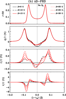
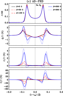
Figure 1: The emergent $I$, $Q/I$, $U/I$, and $V/I$ profiles of a theoretical model line computed with AD-PRD matrix. Atomic parameters of this line correspond to those of the Na i D₂ line. The line-of-sight is at $\mu=0.11$ and $\varphi=0^{\circ}$. A self-emitting isothermal slab with model parameters $(T,\,\Delta\lambda_{\rm D},\,\epsilon,\,r)=(100,\,25\,{\rm m}$Å,$\,10^{-4},\,10^{-7})$ is considered. The magnetic field orientation $(\vartheta_{B},\varphi_{B})=(90^{\circ},45^{\circ})$. The field strength is varied in the range 0 to 300 G.

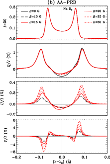
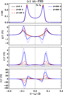
Figure 2: Same as Fig. 1, but computed with AA-PRD matrix.

Figure 3: A comparison of emergent $I$, $Q/I$, $U/I$, and $V/I$ profiles computed using AD-PRD (solid lines) and AA-PRD (dashed lines) matrices. Atomic parameters of the theoretical model line correspond to those of the Na i D₂ line. The line-of-sight is at $\mu=0.11$ and $\varphi=0^{\circ}$. A self-emitting isothermal slab with model parameters $(T,\,\Delta\lambda_{\rm D},\,\epsilon,\,r)=(100,\,25\,{\rm m}$Å,$\,10^{-4},\,10^{-7})$ is considered. The magnetic field orientation $(\vartheta_{B},\varphi_{B})=(90^{\circ},45^{\circ})$. Panel (a) corresponds to $B=3$ G, panel (b) to $B=5$ G, and panel (c) to $B=10$ G.

Figure 4: Same as Fig. 3, but for $B=15$ G in panel (a), $B=30$ G in panel (b), and $B=200$ G in panel (c).

Figure 5: A comparison of total degree of surface linear polarization $P$ computed using AD-PRD (solid lines) and AA-PRD (dashed lines) matrices. Atomic parameters of the theoretical model line correspond to those of the Na i D₂ line. The line-of-sight is at $\mu=0.11$ and $\varphi=0^{\circ}$. A self-emitting isothermal slab with model parameters $(T,\,\Delta\lambda_{\rm D},\,\epsilon,\,r)=(100,\,25\,{\rm m}$Å,$\,10^{-4},\,10^{-7})$ is considered. The magnetic field orientation $(\vartheta_{B},\varphi_{B})=(90^{\circ},45^{\circ})$. Panel (a) corresponds to $B=5$ G, panel (b) to $B=10$ G, panel (c) to $B=15$ G, and panel (d) to $B=30$ G.

3.1 Field Strength Variations

Figure 6: A comparison of emergent $I$, $Q/I$, $U/I$, and $V/I$ profiles computed using AD-PRD (solid lines) and AA-PRD (dashed lines) matrices. Atomic parameters of the theoretical model line correspond to those of the Na i D₂ line. A self-emitting isothermal slab with model parameters $(T,\,\Delta\lambda_{\rm D},\,\epsilon,\,r)=(100,\,25\,{\rm m}$Å,$\,10^{-4},\,10^{-7})$ is considered. The magnetic field parameters are $(B,\,\vartheta_{B},\,\varphi_{B})=(5\,{\rm G},\,90^{\circ},\,45^{\circ})$. Panel (a) corresponds to $\mu=0.297$ and panel (b) to $\mu=0.5$.

Figure 7: Same as Figure 6, but for $\mu=0.7$ in panel (a) and $\mu=0.97$ in panel (b).

Figures 1 and 2 show the emergent Stokes profiles computed with AD-PRD and AA-PRD matrices respectively, for a range of field strengths between 0 and 300 G. We first discuss the influence of field strength variation on the emergent Stokes profiles. A self-reversed emission profile typical of a self-emitting slab of $T=100$ (see e.g., Faurobert, 1987) is seen in Stokes $I$. The magnetic splitting of the HFS components remains much smaller than the chosen Doppler width of 25 mÅ for fields up to 100 G. With further increase in field strength to 300 G the magnetic splitting starts to become comparable and slightly larger than the chosen Doppler width. Consequently, the Stokes $I$ profiles remain nearly insensitive to variations in $B$, except for fields larger than 100 G when we start to see slight magnetic broadening (see blue lines in the Stokes $I$ panel of Figs. 1(c) and 2(c)). For the case of realistic solar atmosphere, with a typical Doppler width of about 40 mÅ the magnetic splittings remain much smaller than the Doppler width for the entire range of field strengths considered in the present paper.

Asymmetric displacements of the hyperfine structure states about the parent $J$ state (see Figs. 1(g) and 1(i) of Sampoorna et al., 2019a) give rise to a very slight asymmetry in the wing peaks of non-magnetic $Q/I$ profile (see black solid line in $Q/I$ panel of Figs. 1 and 2). This asymmetry in the wing peaks of $Q/I$ continues to exist for fields as large as 300 G. For fields below 200 G this asymmetry may be attributed to the non-linear splitting of HFS magnetic components in the incomplete PBE regime. However, for fields larger than 200 G it may be due to the fact that although the upper level of Na i D₂ line enters the complete PBE regime, the lower level continues to be in the incomplete PBE regime. For the same reasons, the $U/I$ profiles are also asymmetric about the line center. For $B<50$ G the blue wing peak of $U/I$ is smaller in amplitude than the red wing peak. This is reversed for $B>50$ G.

In the line cores of $Q/I$ and $U/I$ profiles, we see depolarization and rotation for fields in the range $0<B<10$ G. These are due to the Hanle effect. For $10\leqslant B\leqslant 50$ G, we see the signatures of level-crossings in the line cores of ($Q/I$, $U/I$) profiles, namely they tend towards the non-magnetic value (see Figs. 1(b) and 2(b)). We recall that, traditionally the loops in the polarization diagram (namely, a plot of $Q/I$ versus $U/I$ for a given wavelength and for a range of magnetic field strength or orientation values) are identified to be due to the level-crossings in the incomplete PBE regime (see e.g., Bommier, 1980; Landi Degl’Innocenti & Landolfi, 2004, see also Sowmya et al. 2014). When a given curve in the polarization diagram forms a loop the $Q/I$ and $U/I$ values tend towards the non-magnetic value. Based on this we identify the above noted behavior in the line cores of ($Q/I$, $U/I$) profiles for the mentioned field strength regime as to be the signatures of level-crossings in the incomplete PBE regime. Polarization diagrams require the use of very fine grids of magnetic field strength or orientation. With the radiative transfer calculations presented in this paper, it is computationally difficult to produce such diagrams. For $B>50$ G, transverse Zeeman effect like signatures are seen in the line core of ($Q/I$, $U/I$) profiles (see Figs. 1(c) and 2(c)). The Faraday rotation (del Pino Alemán et al., 2016; Alsina Ballester et al., 2017; Sampoorna et al., 2017), which results in depolarization in the wings of $Q/I$ and generation of $U/I$ in the wings, strongly influences the wings of $U/I$ profiles for the entire field strength regime considered here, while it shows up in $Q/I$ for $B\geqslant 30$ G. For the cases of theoretical model line and the isothermal model atmosphere considered in this section, the Voigt effect starts to show up in $U/I$ for $B\geqslant 50$ G and in $Q/I$ for $B\geqslant 100$ G, and its signatures are similar to those discussed in Sampoorna et al. (2019a). Also we see the signatures of incomplete PBE in the $V/I$ profiles, which are now asymmetric about the line center for fields up to 30 G.

The above discussions concerning the influence of field strength variation on the Stokes profiles are valid for both AD-PRD and AA-PRD cases. We now discuss the similarities or differences between the Stokes profiles computed with AD-PRD and AA-PRD matrices. In the absence of magnetic fields, the Stokes profiles computed with AD-PRD and AA-PRD do not differ greatly (compare black solid lines in Figs. 1 and 2). In fact the differences are ignorable (as shown also in Supriya et al., 2013b). However, in the presence of magnetic fields, differences are significant particularly in the $U/I$ profiles (compare Figs. 1 and 2). Similar results have also been obtained by Nagendra et al. (2002), Nagendra & Sampoorna (2011), and Sampoorna et al. (2017) for the case of a two-level atom without HFS. In the present case of two-level atom with HFS and for the isothermal model atmosphere considered in this section, the differences in $(Q/I,U/I)$ profiles for AD-PRD and AA-PRD cases are significant for fields up to 30 G, after which the differences decrease and nearly vanish for $B\geqslant 200$ G. For easier comparison, the above is illustrated in Figs. 3 and 4. For $B\leqslant 30$ G the magnitude of $U/I$ is comparable to the corresponding magnitude of $Q/I$ in the line core. For example for $B=5$ G and AD-PRD case (solid lines in Fig. 3(b)), the magnitudes of $Q/I$ and $U/I$ at the line center are respectively 0.33% and 0.16%. Given this, the differences between the AD-PRD and AA-PRD solutions are relatively smaller in amplitude for the case of $Q/I$ than in the case of $U/I$. Moreover, the relative changes in profile shape are significantly larger for $U/I$ profiles than the $Q/I$ profiles, demonstrating the sensitivity of $U/I$ profiles to the AD-PRD effects. These differences between the AD-PRD and AA-PRD solutions persist in the line core, even if one considers the total degree of linear polarization $P=\sqrt{Q^{2}+U^{2}}/I$ (see Fig. 5). In the line wings, since $Q/I$ is about an order of magnitude larger than the $U/I$ (see e.g., Fig. 3), the differences in $P$ for the AD-PRD and AA-PRD cases are similar to those seen in the corresponding case of $Q/I$. Finally, we note from Figs. 3 and 4 that for the considered model, the Stokes $I$ and $V/I$ profiles are somewhat insensitive to the choice of the magnetic PRD function, while the $Q/I$ and $U/I$ profiles are highly sensitive for $B\leqslant 30$ G. Since $U/I$ is generated by the breaking of axi-symmetry of the problem, it is relatively more sensitive to AD-PRD effects than the $Q/I$.

Figure 8: A comparison of emergent $I$, $Q/I$, $U/I$, and $V/I$ profiles computed using AD-PRD (solid lines) and AA-PRD (dashed lines) matrices. Atomic parameters of the theoretical model line correspond to those of the Na i D₂ line. The line-of-sight is at $\mu=0.11$ and $\varphi=0^{\circ}$. A self-emitting isothermal slab with model parameters $(T,\,\Delta\lambda_{\rm D},\,\epsilon,\,r)=(100,\,25\,{\rm m}$Å,$\,10^{-4},\,10^{-7})$ is considered. The magnetic field parameters are $(B,\,\vartheta_{B},\,\varphi_{B})=(5\,{\rm G},\,0^{\circ},\,0^{\circ})$.

3.2 Center-to-limb Variations

A comparison of emergent Stokes profiles computed with AD-PRD and AA-PRD matrices for a fixed field strength of $B=5$ G and for different values of the cosine of the helio-centric angle, namely $\mu$, is shown in Figures 6 and 7. With the increasing values of $\mu$ the intensity slightly increases, while the polarization decreases as expected. It is interesting to note that the decrease in $Q/I$ when $\mu$ changes from $0.297$ to $0.5$ is somewhat small. This is due to the choice of a self-emitting isothermal atmosphere with $T=100$. In the case of AD-PRD, the peak in $U/I$ around $0.08$ Å changes sign for $\mu=0.5$ and then increases in magnitude when $\mu$ further increases. Such a behavior was also noted in the case of two-level atom without HFS by Nagendra & Sampoorna (2011). The differences between the $Q/I$ profiles computed with AD-PRD and AA-PRD matrices decrease when $\mu$ increases except for $\mu=0.97$ (see Fig. 7(b)). In the case of $U/I$ the differences increase as $\mu\to 1$. In fact the $U/I$ computed with AD-PRD exhibits a stronger dependence on $\mu$ than that computed with AA-PRD. As for the $V/I$ the small differences seen near the line center show a slight increase as $\mu\to 1$.

3.3 The Case of Vertical Magnetic Field

Nagendra et al. (2002, see also ) showed that when AD-PRD matrix for Hanle effect (given by Approximation-II of Bommier, 1997) is used in the solution of the polarized radiative transfer equation, non-zero Stokes $U$ can be generated even if the magnetic field is oriented along the symmetry axis of the slab (namely, the atmospheric normal). In Figure 8, we present a comparison of emergent Stokes profiles computed with AD-PRD and AA-PRD matrices for this interesting case of vertical magnetic field. The Hanle effect which operates in the line core is expected to vanish for vertical fields. This is indeed the case, when AA-PRD matrix is used (see dashed lines in Fig. 8). In fact the Stokes $U/I$ is zero in the line core where the Hanle effect operates, while in the wings where Faraday rotation operates the $U/I$ is on the order of 0.0075 % which is not visible in the scale adopted. Also Stokes $Q/I$ is identical to the corresponding zero field case (compare black solid line in Fig. 2 and dashed line in Fig. 8). Such a small contribution from Faraday rotation to the wings of ($Q/I$, $U/I$) profiles is due to the choice of $T=100$. For larger optical thickness (like in the case of semi-infinite atmospheres) contribution from Faraday rotation even for a very inclined line-of-sight and a vertical magnetic field case would be large enough to be noticeable (see e.g., Fig. 3 of Alsina Ballester et al., 2016).

When AD-PRD matrix is used the Stokes $Q/I$ continues to nearly coincide with the corresponding zero field case (compare black solid lines in Figs. 1 and 8). However, a non-zero Stokes $U/I$ is generated both in the line core and near wings (see solid line in Fig. 8). As already noted above, in this case the contribution from the Faraday rotation to the wings of $U/I$ is less than 0.01 %. Thus in the present case the non-zero $U/I$ is entirely due to the use of AD-PRD matrix. For larger values of $T$, we may expect that AD-PRD effects would generate a non-zero $U/I$ in the line core, while both AD-PRD and Faraday rotation would contribute to the line wings. As shown in detail in Frisch et al. (2001), it is the azimuth ($\varphi-\varphi^{\prime}$) dependence of the AD-PRD functions that give rise to non-zero $U/I$ in the present axisymmetric case of a vertical field. More specifically, the azimuthal Fourier coefficients of AD-PRD function (cf. Domke & Hubeny, 1988; Frisch, 2009) with order other than zero are responsible for the generation of non-zero Stokes $U$ in the presence of a weak vertical magnetic field (Frisch et al., 2001, see also Supriya et al. 2013a).

Figure 9: Effect of variation of elastic collision rate $\Gamma_{\rm E}/\Gamma_{\rm R}$ on the emergent $I$, $Q/I$, $U/I$, and $V/I$ profiles computed using AD-PRD (panel (a)) and AA-PRD (panel (b)) matrices. Atomic parameters of the theoretical model line correspond to those of the Na i D₂ line. The line-of-sight is at $\mu=0.11$ and $\varphi=0^{\circ}$. A self-emitting isothermal slab with model parameters $(T,\,\Delta\lambda_{\rm D},\,\epsilon,\,r)=(100,\,25\,{\rm m}$Å,$\,10^{-4},\,10^{-7})$ is considered. The magnetic field parameters $(B,\,\vartheta_{B},\,\varphi_{B})=(10\,{\rm G},\,90^{\circ},\,45^{\circ})$.

4 Effect of Elastic Collisions on Emergent Stokes Profiles

The PRD matrix, for scattering on a two-level atom with HFS including the incomplete PBE regime of field strength, derived in Sowmya et al. (2014) using a Kramers-Heisenberg scattering approach (Stenflo, 1994) considered only the collissionless case. The collisional PRD matrix was derived recently in Bommier (2017, see also ) using a quantum electrodynamic (QED) approach. She considers the case of a two-term atom with and without HFS. The collisional PRD matrix for a two-level atom with HFS can be obtained from the PRD matrix for two-term atom without HFS by using simple quantum number replacement. For clarity, we present the resulting collisional PRD matrix in Appendix A. As noted in Appendix A, for computational simplicity the type-III AD-PRD function is approximated by the complete frequency redistribution (see Eqs. (A60)–(A63)). For the case of a two-level atom without HFS, Sampoorna et al. (2017) show that such an approximation may introduce small errors for weak fields when the medium is moderately thick (see their Fig. 1(a)). For the case of a two-level atom with HFS, validating this approximation would be beyond the scope of the available computing resources.

In a realistic solar model atmosphere such as the model C of Fontenla et al. (1993), the elastic collision rate $\Gamma_{\rm E}$ is known to vary approximately in the range of $2\times 10^{9}$ s^-1 at the base of the photosphere to $10^{2}$ s^-1 at the outermost layers of the chromosphere. For the Na i D₂ line the radiative de-excitation rate $\Gamma_{\rm R}$ of the upper level is $6.3\times 10^{7}$ s^-1. Therefore, here we vary $\Gamma_{\rm E}/\Gamma_{\rm R}$ in the range 0 and 30. Figure 9 shows the influence of variation of $\Gamma_{\rm E}/\Gamma_{\rm R}$ on the emergent Stokes profiles computed with AD-PRD (panel (a)) and AA-PRD (panel (b)) matrices. With the increasing elastic collision rate, the total damping width of the line given by $a=(\Gamma_{\rm R}+\Gamma_{\rm I}+\Gamma_{\rm E})/(4\pi\Delta{\nu_{\rm D}})$ also increases. Therefore, the Stokes $I$ profiles become progressively broader, while the Stokes $Q/I$, $U/I$, and $V/I$ profiles exhibit a depolarization as expected. This behavior is common to Stokes profiles computed with both AD-PRD and AA-PRD. Comparing panels (a) and (b) of Fig. 9, we see that the differences between the solutions computed with AD-PRD and AA-PRD are the largest for $\Gamma_{\rm E}/\Gamma_{\rm R}=0$. As the elastic collision rate increases these differences decrease. For $\Gamma_{\rm E}/\Gamma_{\rm R}$ up to 1 the differences are noticeable, beyond which they become ignorable.

5 Conclusions

In the present paper we solve the problem of polarized line formation in a magnetized isothermal self-emitting planar atmosphere including angle-dependent PRD in scattering on a two-level atom with HFS. For this purpose we take the example of an atomic system corresponding to Na i D₂ line. Since the computational requirements with AD-PRD are significantly larger than those with AA-PRD, we consider a self-emitting slab of moderate optical thickness (namely, $T=100$) for our studies. We consider a range of field strengths from 0 to 300 G. The influence of field strength variation on the emergent Stokes profiles is similar for both AD-PRD and AA-PRD. Therefore, the signatures of incomplete PBE, Faraday rotation, Voigt effect, and PRD as noted in the angle-averaged case (cf. Sampoorna et al., 2019a) also remain valid for the angle-dependent case.

The computationally simpler AA-PRD idealization is sufficient to accurately calculate the emergent Stokes profiles in the absence of magnetic fields (see also Supriya et al., 2013b). However, in the presence of magnetic fields, the use of computationally very demanding AD-PRD cannot be avoided. In fact, we show that the AD-PRD effects are significant particularly in the $U/I$ profiles. This is true in the case of two-level atom without HFS (cf. Nagendra et al., 2002; Nagendra & Sampoorna, 2011; Sampoorna et al., 2017), and also in the present case of two-level atom with HFS. As demonstrated in Fig. 5, the AD-PRD effects continue to be significant in the line core of total degree of linear polarization for weaker fields. This is because for fields up to 30 G, the magnitudes of $U/I$ and the corresponding line core $Q/I$ are comparable. For the theoretical model line and model atmosphere considered in the present paper, the AD-PRD effects need to be included in the computation of the emergent Stokes profiles for field strengths up to 30 G. For fields larger than 30 G, one can continue to use the idealization of AA-PRD. Furthermore, we show that the AD-PRD effects are prominent when elastic collisions are negligible or small compared to the radiative de-excitation rate. Since several of the strong resonance lines form in the upper chromosphere where elastic collisions are expected to be typically small (relative to the Einstein coefficient), the full treatment of AD-PRD becomes essential for an accurate modeling of spectral lines formed in weakly magnetized atmospheres.

Appendix A Collisional PRD Matrix in the Incomplete PBE Regime

The collisional PRD matrix for a two-term atom without HFS and in the incomplete PBE regime is given in Equation (A.1) of Bommier (2017, 2018). By using the following quantum number replacement

$$L\to J;\quad J\to F;\quad S\to I;\quad J^{\ast}\to F^{\ast}$$

in Equation (A.1) of Bommier (2018), we obtain the collisional PRD matrix for a two-level atom with HFS. In the above equation, $L$ is the orbital angular momentum quantum number, $J$ is the total electronic angular momentum quantum number, $S$ is the electronic spin, $I$ is the nuclear spin, and $F$ is the quantum number resulting from $J$–$I$ coupling. In the incomplete PBE regime $F$ is not a good quantum number, while the magnetic quantum number $M$ continues to be a good quantum number. Thus the modified quantum number $F^{\ast}$ labels the different states spanned by the quantum numbers ($J$, $I$, $M$). In the atomic rest frame and for a magnetic field vector ${\bm{B}}$ along the Z-axis, the resulting collisional PRD matrix for a two-level atom with HFS in the notations of Bommier (2017) is given by

$$\!\!\!\!\!\!\!\!\!\!{\mathcal{R}}_{ij}(\tilde{\nu},\tilde{\nu}_{1},{\bm{\Omega}},{\bm{\Omega}}_{1};{\bm{B}})=\sum_{KK^{\prime}Q}{\mathcal{T}}^{K}_{Q}(i,{\bm{\Omega}})(-1)^{Q}{\mathcal{T}}^{K^{\prime}}_{-Q}(j,{\bm{\Omega}}_{1})$$

$$\!\!\!\!\!\!\!\!\!\!\times\frac{3(2J_{u}+1)}{(2I+1)}\sqrt{(2K+1)(2K^{\prime}+1)}\sum_{F_{u}\bar{F}_{u}F^{\ast}_{u}M_{u}F^{\prime}_{u}\bar{F}^{\prime}_{u}F^{\prime\ast}_{u}M^{\prime}_{u}}$$

$$\!\!\!\!\!\!\!\!\!\!\times\sum_{F_{l}\bar{F}_{l}F^{\ast}_{l}M_{l}F^{\prime}_{l}\bar{F}^{\prime}_{l}F^{\prime\ast}_{l}M^{\prime}_{l}}\!\!\!\!\!\!\!\!\!\!\!\!\!\!\!\!\!\!(-1)^{M_{l}-M^{\prime}_{l}}(-1)^{F_{u}+\bar{F}_{u}+F^{\prime}_{u}+\bar{F}^{\prime}_{u}}(-1)^{F_{l}+\bar{F}_{l}+F^{\prime}_{l}+\bar{F}^{\prime}_{l}}$$

$$\!\!\!\!\!\!\!\!\!\!\times\sqrt{(2F_{u}+1)(2\bar{F}_{u}+1)(2F^{\prime}_{u}+1)(2\bar{F}^{\prime}_{u}+1)}$$

$$\!\!\!\!\!\!\!\!\!\!\times\sqrt{(2F_{l}+1)(2\bar{F}_{l}+1)(2F^{\prime}_{l}+1)(2\bar{F}^{\prime}_{l}+1)}$$

$$\!\!\!\!\!\!\!\!\!\!\times C^{F_{u}}_{F^{\ast}_{u}M_{u}}(B)C^{\bar{F}_{u}}_{F^{\ast}_{u}M_{u}}(B)C^{F^{\prime}_{u}}_{F^{\prime\ast}_{u}M^{\prime}_{u}}(B)C^{\bar{F}^{\prime}_{u}}_{F^{\prime\ast}_{u}M^{\prime}_{u}}(B)$$

$$\!\!\!\!\!\!\!\!\!\!\times C^{F_{l}}_{F^{\ast}_{l}M_{l}}(B)C^{\bar{F}_{l}}_{F^{\ast}_{l}M_{l}}(B)C^{F^{\prime}_{l}}_{F^{\prime\ast}_{l}M^{\prime}_{l}}(B)C^{\bar{F}^{\prime}_{l}}_{F^{\prime\ast}_{l}M^{\prime}_{l}}(B)$$

$$\!\!\!\!\!\!\!\!\!\!\times\left\{\begin{array}[]{ccc}F_{u}&1&F_{l}\\ J_{l}&I&J_{u}\\ \end{array}\right\}\left\{\begin{array}[]{ccc}F^{\prime}_{u}&1&\bar{F}_{l}\\ J_{l}&I&J_{u}\\ \end{array}\right\}\left\{\begin{array}[]{ccc}\bar{F}_{u}&1&F^{\prime}_{l}\\ J_{l}&I&J_{u}\\ \end{array}\right\}\left\{\begin{array}[]{ccc}\bar{F}^{\prime}_{u}&1&\bar{F}^{\prime}_{l}\\ J_{l}&I&J_{u}\\ \end{array}\right\}$$ (A9)

$$\!\!\!\!\!\!\!\!\!\!\times\left(\begin{array}[]{ccc}F_{u}&1&F_{l}\\ -M_{u}&p&M_{l}\\ \end{array}\right)\left(\begin{array}[]{ccc}F^{\prime}_{u}&1&\bar{F}_{l}\\ -M^{\prime}_{u}&p^{\prime}&M_{l}\\ \end{array}\right)\left(\begin{array}[]{ccc}\bar{F}_{u}&1&F^{\prime}_{l}\\ -M_{u}&p^{\prime\prime\prime}&M^{\prime}_{l}\\ \end{array}\right)$$ (A16)

$$\!\!\!\!\!\!\!\!\!\!\times\left(\begin{array}[]{ccc}\bar{F}^{\prime}_{u}&1&\bar{F}^{\prime}_{l}\\ -M^{\prime}_{u}&p^{\prime\prime}&M^{\prime}_{l}\\ \end{array}\right)\left(\begin{array}[]{ccc}1&1&K^{\prime}\\ -p&p^{\prime}&Q\\ \end{array}\right)\left(\begin{array}[]{ccc}1&1&K\\ -p^{\prime\prime\prime}&p^{\prime\prime}&Q\\ \end{array}\right)$$ (A23)

$$\!\!\!\!\!\!\!\!\!\!\times\Bigg{\{}{\frac{\Gamma_{\rm R}}{\Gamma_{\rm R}+\Gamma_{\rm I}+\Gamma_{\rm E}+{\rm i}{\Delta E_{M_{u}M^{\prime}_{u}}\over\hbar}}}\delta(\tilde{\nu}-\tilde{\nu}_{1}-\nu_{M_{l}M^{\prime}_{l}})$$

$$\!\!\!\!\!\!\!\!\!\!\times{1\over 2}\left[\Phi_{ba}(\nu_{M^{\prime}_{u}M_{l}}-\tilde{\nu}_{1})+\Phi^{\ast}_{ba}(\nu_{M_{u}M_{l}}-\tilde{\nu}_{1})\right]$$

$$\!\!\!\!\!\!\!\!\!\!+\left[{\frac{\Gamma_{\rm R}}{\Gamma_{\rm R}+\Gamma_{\rm I}+{\rm i}{\Delta E_{M_{u}M^{\prime}_{u}}\over\hbar}}}-{\frac{\Gamma_{\rm R}}{\Gamma_{\rm R}+\Gamma_{\rm I}+\Gamma_{\rm E}+{\rm i}{\Delta E_{M_{u}M^{\prime}_{u}}\over\hbar}}}\right]$$

$$\!\!\!\!\!\!\!\!\!\!\times{1\over 2}\left[\Phi_{ba}(\nu_{M^{\prime}_{u}M_{l}}-\tilde{\nu}_{1})+\Phi^{\ast}_{ba}(\nu_{M_{u}M_{l}}-\tilde{\nu}_{1})\right]$$

$$\!\!\!\!\!\!\!\!\!\!\times{1\over 2}\left[\Phi_{ba}(\nu_{M^{\prime}_{u}M^{\prime}_{l}}-\tilde{\nu})+\Phi^{\ast}_{ba}(\nu_{M_{u}M^{\prime}_{l}}-\tilde{\nu})\right]\Bigg{\}},$$ (A24)

where $i,j=0,1,2,3$ (corresponding to $I$, $Q$, $U$, and $V$), $\tilde{\nu}$ and $\tilde{\nu}_{1}$ are respectively the frequencies of the scattered and incident rays in the atomic frame, ${\bm{\Omega}}$ and ${\bm{\Omega}}_{1}$ refer respectively to the scattered and incident ray directions with respect to the magnetic field, $\Gamma_{\rm R}$ denotes the radiative de-excitation rate of the upper level, $\Gamma_{\rm I}$ the inelastic de-excitation rate, and $\Gamma_{\rm E}$ the elastic collisional rate. $\mathcal{T}^{K}_{Q}(i,{\bm{\Omega}})$ are the irreducible spherical tensors with $K=0,1,2$ and $-K\leqslant Q\leqslant+K$ (see Landi Degl’Innocenti, 1984). The profile function $\Phi_{ba}$ is defined in Eq. (2) of Bommier (1997). All the other symbols appearing in the above equation are defined in Bommier (2017).

When $\Gamma_{\rm E}=0$, Eq. (A24) can be shown to be equivalent to the collissionless PRD matrix derived in Sowmya et al. (2014). To make this equivalence transparent and also as we prefer to work with the notations of Sowmya et al. (2014), in the following we give the equivalence between the symbols used in Sowmya et al. (2014, see also ) and those used in Bommier (2017). First, we identify our notations for the different quantum numbers with those used by Bommier (2017), namely, $J_{a}=J_{l}$, $J_{b}=J_{u}$, $I_{s}=I$, $i_{a}=F^{\ast}_{l}$, $i_{f}=F^{\prime\ast}_{l}$, $i_{b}=F^{\ast}_{u}$, $i_{b^{\prime}}=F^{\prime\ast}_{u}$, $m_{a}=M_{l}$, $m_{f}=M^{\prime}_{l}$, $m_{b}=M_{u}$, $m_{b^{\prime}}=M^{\prime}_{u}$, $F_{a}=F_{l}$, $F_{a^{\prime}}=\bar{F}_{l}$, $F_{f}=F^{\prime}_{l}$, $F_{f^{\prime}}=\bar{F}^{\prime}_{l}$, $F_{b^{\prime\prime}}=F_{u}$, $F_{b}=\bar{F}_{u}$, $F_{b^{\prime\prime\prime}}=F^{\prime}_{u}$, $F_{b^{\prime}}=\bar{F}^{\prime}_{u}$, $-q=p^{\prime\prime\prime}$, $-q^{\prime}=p^{\prime\prime}$, $-q^{\prime\prime}=p$, and $-q^{\prime\prime\prime}=p^{\prime}$. We note that in Sowmya et al. (2014) the symbol $\mu$ was used for magnetic quantum number, which has been changed to $m$ in the present paper as $\mu$ is used to denote the line-of-sight. With the above identification and from the properties of 3-$j$ symbols it can be shown that the sign factor $(-1)^{m_{a}-m_{f}}$ is the same as $(-1)^{q-q^{\prime\prime\prime}+Q}$. The other two sign factors appearing in Eq. (A24) vanish when we express the first four 3-$j$ symbols in Eq. (A24) in a form given by the corresponding 3-$j$ symbols in Eq. (A57) below. We next identify that $C^{F}_{F^{\ast}M}(B)$ appearing in Eq. (A24) is the same as $C^{i}_{F}(JI_{s},m)$ used in Sowmya et al. (2014). We now consider the first term of the big flower bracket in Eq. (A24). Here the energy difference $\Delta E_{M_{u}M^{\prime}_{u}}$ in our notations is given by $\Delta E_{m_{b}m_{b^{\prime}}}=E_{i_{b}}(J_{b}I_{s},m_{b})-E_{i_{b^{\prime}}}(J_{b}I_{s},m_{b^{\prime}})$, where $E$ denotes the energy shift of a magnetic substate about the energy of the parent $J$ state (see Sowmya et al., 2014, for details). Defining the branching ratio $A$ as

$$A={\Gamma_{\rm R}\over\Gamma_{\rm R}+\Gamma_{\rm I}+\Gamma_{\rm E}},$$ (A25)

and the angle $\alpha$ as

$$\tan\alpha_{i_{b^{\prime}}m_{b^{\prime}}i_{b}m_{b}}={\Delta E_{m_{b^{\prime}}m_{b}}\over\hbar(\Gamma_{\rm R}+\Gamma_{\rm I}+\Gamma_{\rm E})},$$ (A26)

it can be shown that

$${\Gamma_{\rm R}\over\Gamma_{\rm R}+\Gamma_{\rm I}+\Gamma_{\rm E}+{\rm i}{\Delta E_{m_{b}m_{b^{\prime}}}\over\hbar}}=A\cos\alpha_{i_{b^{\prime}}m_{b^{\prime}}i_{b}m_{b}}{\rm e}^{{\rm i}\alpha_{i_{b^{\prime}}m_{b^{\prime}}i_{b}m_{b}}}.$$ (A27)

The symbol $\beta$ defined in Sowmya et al. (2014) is changed to symbol $\alpha$ for consistency with the previous papers (see e.g., Sampoorna et al., 2017). The profile function $\Phi_{\gamma}(\nu_{i_{b}m_{b}i_{a}m_{a}}-\xi^{\prime})$ defined in Sowmya et al. (2014, see their Eqs. (13) and (14)) can be shown to be a complex conjugate of $\Phi_{ba}$ defined in Eq. (2) of Bommier (1997), after noting that $\xi^{\prime}=\tilde{\nu}_{1}$ and identifying that the damping constant $\gamma$ is equal to $\Gamma_{\rm R}+\Gamma_{\rm I}+\Gamma_{\rm E}$. We next consider the term in the square bracket of Eq. (A24). This term can be re-written as

$${\Gamma_{\rm E}\over\Gamma_{\rm R}+\Gamma_{\rm I}+\Gamma_{\rm E}+{\rm i}{\Delta E_{m_{b}m_{b^{\prime}}}\over\hbar}}\ {\Gamma_{\rm R}\over\Gamma_{\rm R}+\Gamma_{\rm I}+{\rm i}{\Delta E_{m_{b}m_{b^{\prime}}}\over\hbar}}.$$ (A28)

We define the angle $\beta$ as

$$\tan\beta_{i_{b^{\prime}}m_{b^{\prime}}i_{b}m_{b}}={\Delta E_{m_{b^{\prime}}m_{b}}\over\hbar(\Gamma_{\rm R}+\Gamma_{\rm I})}.$$ (A29)

Using Eqs. (A26) and (A29), Eq. (A28) can be re-written as

$${\Gamma_{\rm E}\over\Gamma_{\rm R}+\Gamma_{\rm I}+\Gamma_{\rm E}}\cos\alpha_{i_{b^{\prime}}m_{b^{\prime}}i_{b}m_{b}}{\rm e}^{{\rm i}\alpha_{i_{b^{\prime}}m_{b^{\prime}}i_{b}m_{b}}}\ {\Gamma_{\rm R}\over\Gamma_{\rm R}+\Gamma_{\rm I}}\cos\beta_{i_{b^{\prime}}m_{b^{\prime}}i_{b}m_{b}}{\rm e}^{{\rm i}\beta_{i_{b^{\prime}}m_{b^{\prime}}i_{b}m_{b}}}.$$ (A30)

Defining the branching ratio $B$ as

$$B={\Gamma_{\rm R}\over\Gamma_{\rm R}+\Gamma_{\rm I}}\ {\Gamma_{\rm E}\over\Gamma_{\rm R}+\Gamma_{\rm I}+\Gamma_{\rm E}},$$ (A31)

the term in the square bracket of Eq. (A24) reduces to

$$B\cos\alpha_{i_{b^{\prime}}m_{b^{\prime}}i_{b}m_{b}}\cos\beta_{i_{b^{\prime}}m_{b^{\prime}}i_{b}m_{b}}{\rm e}^{{\rm i}(\alpha_{i_{b^{\prime}}m_{b^{\prime}}i_{b}m_{b}}+\beta_{i_{b^{\prime}}m_{b^{\prime}}i_{b}m_{b}})}.$$

Assuming Maxwellian velocity distribution and transforming to the laboratory frame and the atmospheric reference frame (wherein $Z$-axis is along the normal to the atmosphere, see e.g., Sampoorna et al., 2017) we obtain the collisional PRD matrix for a two-level atom with HFS and in the incomplete PBE regime as

$$\!\!\!\!\!\!\!{R}_{ij}(x,{\bm{n}},x^{\prime},{\bm{n}}^{\prime},{\bm{B}})=\sum_{KQ}{\mathcal{T}}^{K}_{Q}(i,{\bm{n}})\sum_{K^{\prime}Q^{\prime}}$$

$$\!\!\!\!\!\!\!\times N^{K,K^{\prime}}_{QQ^{\prime}}(x,x^{\prime},\Theta,{\bm{B}})(-1)^{Q^{\prime}}{\mathcal{T}}^{K^{\prime}}_{-Q^{\prime}}(j,{\bm{n}}^{\prime}),$$ (A32)

where $x$ and $x^{\prime}$ are the non-dimensional frequencies of the scattered and incident rays respectively, ${\bm{n}}(\vartheta,\varphi)$ and ${\bm{n}}^{\prime}(\vartheta^{\prime},\varphi^{\prime})$ refer respectively to the scattered and incident ray directions with respect to the atmospheric normal, and $\Theta$ denotes the scattering angle between the incident and scattered rays. The vector magnetic field is denoted by ${\bm{B}}$ with field strength $B$, inclination $\vartheta_{B}$, and azimuth $\varphi_{B}$ about the atmospheric normal. The magnetic kernel has the form

$$\!\!\!\!\!\!\!\!\!\!\!\!\!\!\!\!N^{K,K^{\prime}}_{QQ^{\prime}}(x,x^{\prime},\Theta,{\bm{B}})={\rm e}^{{\rm i}(Q^{\prime}-Q)\varphi_{B}}\sum_{Q^{\prime\prime}}d^{K}_{QQ^{\prime\prime}}(\vartheta_{B})$$

$$\!\!\!\!\!\!\!\!\!\!\!\!\!\!\!\!\times{\mathcal{R}}^{K,K^{\prime}}_{Q^{\prime\prime}}(x,x^{\prime},\Theta,B)d^{K^{\prime}}_{Q^{\prime\prime}Q^{\prime}}(-\vartheta_{B})\,,$$ (A33)

where the symbol $d^{K}_{QQ^{\prime}}(\vartheta_{B})$ stands for the elements of reduced rotation matrices, which are tabulated in Table 2.1 of Landi Degl’Innocenti & Landolfi (2004). The collisional PRD functions ${\mathcal{R}}^{K,K^{\prime}}_{Q^{\prime\prime}}(x,x^{\prime},\Theta,B)$ for the case of a two-level atom with HFS and in the incomplete PBE regime are given by

$$\!\!\!\!\!\!\!\!\!\!{\mathcal{R}}^{K,K^{\prime}}_{Q^{\prime\prime}}(x,x^{\prime},\Theta,B)=\frac{3(2J_{b}+1)}{(2I_{s}+1)}\sqrt{(2K+1)(2K^{\prime}+1)}$$

$$\!\!\!\!\!\!\!\!\!\!\times\sum_{i_{a}m_{a}i_{f}m_{f}i_{b}m_{b}i_{b^{\prime}}m_{b^{\prime}}}\bigg{\{}A\cos\alpha_{i_{b^{\prime}}m_{b^{\prime}}i_{b}m_{b}}{\rm e}^{{\rm i}\alpha_{i_{b^{\prime}}m_{b^{\prime}}i_{b}m_{b}}}$$

$$\!\!\!\!\!\!\!\!\!\!\times[(h^{\rm II}_{i_{b}m_{b},i_{b^{\prime}}m_{b^{\prime}}})_{i_{a}m_{a}i_{f}m_{f}}+{\rm i}(f^{\rm II}_{i_{b}m_{b},i_{b^{\prime}}m_{b^{\prime}}})_{i_{a}m_{a}i_{f}m_{f}}]$$

$$\!\!\!\!\!\!\!\!\!\!+B\cos\alpha_{i_{b^{\prime}}m_{b^{\prime}}i_{b}m_{b}}\cos\beta_{i_{b^{\prime}}m_{b^{\prime}}i_{b}m_{b}}$$

$$\!\!\!\!\!\!\!\!\!\!\times{\rm e}^{{\rm i}(\alpha_{i_{b^{\prime}}m_{b^{\prime}}i_{b}m_{b}}+\beta_{i_{b^{\prime}}m_{b^{\prime}}i_{b}m_{b}})}$$

$$\!\!\!\!\!\!\!\!\!\!\times[(h^{\rm III}_{i_{b}m_{b},i_{b^{\prime}}m_{b^{\prime}}})_{i_{a}m_{a}i_{f}m_{f}}+{\rm i}(f^{\rm III}_{i_{b}m_{b},i_{b^{\prime}}m_{b^{\prime}}})_{i_{a}m_{a}i_{f}m_{f}}]\bigg{\}}$$

$$\!\!\!\!\!\!\!\!\!\!\times\sum_{F_{a}F_{a^{\prime}}F_{f}F_{f^{\prime}}F_{b}F_{b^{\prime}}F_{b^{\prime\prime}}F_{b^{\prime\prime\prime}}}\sum_{qq^{\prime}q^{\prime\prime}q^{\prime\prime\prime}}(-1)^{q-q^{\prime\prime\prime}+Q^{\prime\prime}}$$

$$\!\!\!\!\!\!\!\!\!\!\times\sqrt{(2F_{a}+1)(2F_{f}+1)(2F_{a^{\prime}}+1)(2F_{f^{\prime}}+1)}$$

$$\!\!\!\!\!\!\!\!\!\!\times\sqrt{(2F_{b}+1)(2F_{b^{\prime}}+1)(2F_{b^{\prime\prime}}+1)(2F_{b^{\prime\prime\prime}}+1)}$$

$$\!\!\!\!\!\!\!\!\!\!\times C^{i_{f}}_{F_{f}}(J_{a}I_{s},m_{f})C^{i_{f}}_{F_{f^{\prime}}}(J_{a}I_{s},m_{f})C^{i_{a}}_{F_{a}}(J_{a}I_{s},m_{a})$$

$$\!\!\!\!\!\!\!\!\!\!\times C^{i_{a}}_{F_{a^{\prime}}}(J_{a}I_{s},m_{a})C^{i_{b}}_{F_{b}}(J_{b}I_{s},m_{b})C^{i_{b}}_{F_{b^{\prime\prime}}}(J_{b}I_{s},m_{b})$$

$$\!\!\!\!\!\!\!\!\!\!\times C^{i_{b^{\prime}}}_{F_{b^{\prime}}}(J_{b}I_{s},m_{b^{\prime}})C^{i_{b^{\prime}}}_{F_{b^{\prime\prime\prime}}}(J_{b}I_{s},m_{b^{\prime}})\left\{\begin{array}[]{ccc}J_{a}&J_{b}&1\\ F_{b}&F_{f}&I_{s}\\ \end{array}\right\}$$ (A36)

$$\!\!\!\!\!\!\!\!\!\!\times\left\{\begin{array}[]{ccc}J_{a}&J_{b}&1\\ F_{b^{\prime}}&F_{f^{\prime}}&I_{s}\\ \end{array}\right\}\left\{\begin{array}[]{ccc}J_{a}&J_{b}&1\\ F_{b^{\prime\prime}}&F_{a}&I_{s}\\ \end{array}\right\}\left\{\begin{array}[]{ccc}J_{a}&J_{b}&1\\ F_{b^{\prime\prime\prime}}&F_{a^{\prime}}&I_{s}\\ \end{array}\right\}$$ (A43)

$$\!\!\!\!\!\!\!\!\!\!\times\left(\begin{array}[]{ccc}F_{b}&F_{f}&1\\ -m_{b}&m_{f}&-q\\ \end{array}\right)\left(\begin{array}[]{ccc}F_{b^{\prime}}&F_{f^{\prime}}&1\\ -m_{b^{\prime}}&m_{f}&-q^{\prime}\\ \end{array}\right)\left(\begin{array}[]{ccc}F_{b^{\prime\prime}}&F_{a}&1\\ -m_{b}&m_{a}&-q^{\prime\prime}\\ \end{array}\right)$$ (A50)

$$\!\!\!\!\!\!\!\!\!\!\times\left(\begin{array}[]{ccc}F_{b^{\prime\prime\prime}}&F_{a^{\prime}}&1\\ -m_{b^{\prime}}&m_{a}&-q^{\prime\prime\prime}\\ \end{array}\right)\left(\begin{array}[]{ccc}1&1&K\\ q&-q^{\prime}&Q^{\prime\prime}\\ \end{array}\right)\left(\begin{array}[]{ccc}1&1&K^{\prime}\\ q^{\prime\prime\prime}&-q^{\prime\prime}&-Q^{\prime\prime}\\ \end{array}\right)\,.$$ (A57)

The auxiliary functions $h^{\rm II}$ and $f^{\rm II}$ are defined in Equations (18)–(22) of Sowmya et al. (2014). All the different symbols and quantities appearing in the above equation can be found in the same reference.

The auxiliary functions $h^{\rm III}$ and $f^{\rm III}$ are defined as

$$(h^{\rm III}_{i_{b}m_{b},i_{b^{\prime}}m_{b^{\prime}}})_{i_{a}m_{a}i_{f}m_{f}}$$

$$={1\over 4}\left[R^{\rm III,HH}_{i_{b^{\prime}}m_{b^{\prime}}i_{a}m_{a},i_{b^{\prime}}m_{b^{\prime}}i_{f}m_{f}}+R^{\rm III,HH}_{i_{b^{\prime}}m_{b^{\prime}}i_{a}m_{a},i_{b}m_{b}i_{f}m_{f}}+R^{\rm III,HH}_{i_{b}m_{b}i_{a}m_{a},i_{b^{\prime}}m_{b^{\prime}}i_{f}m_{f}}+R^{\rm III,HH}_{i_{b}m_{b}i_{a}m_{a},i_{b}m_{b}i_{f}m_{f}}\right]$$

$$+{{\rm i}\over 4}\left[R^{\rm III,FH}_{i_{b^{\prime}}m_{b^{\prime}}i_{a}m_{a},i_{b^{\prime}}m_{b^{\prime}}i_{f}m_{f}}+R^{\rm III,FH}_{i_{b^{\prime}}m_{b^{\prime}}i_{a}m_{a},i_{b}m_{b}i_{f}m_{f}}-R^{\rm III,FH}_{i_{b}m_{b}i_{a}m_{a},i_{b^{\prime}}m_{b^{\prime}}i_{f}m_{f}}-R^{\rm III,FH}_{i_{b}m_{b}i_{a}m_{a},i_{b}m_{b}i_{f}m_{f}}\right],$$ (A58)

$$(f^{\rm III}_{i_{b}m_{b},i_{b^{\prime}}m_{b^{\prime}}})_{i_{a}m_{a}i_{f}m_{f}}$$

$$={1\over 4}\left[R^{\rm III,HF}_{i_{b^{\prime}}m_{b^{\prime}}i_{a}m_{a},i_{b^{\prime}}m_{b^{\prime}}i_{f}m_{f}}-R^{\rm III,HF}_{i_{b^{\prime}}m_{b^{\prime}}i_{a}m_{a},i_{b}m_{b}i_{f}m_{f}}+R^{\rm III,HF}_{i_{b}m_{b}i_{a}m_{a},i_{b^{\prime}}m_{b^{\prime}}i_{f}m_{f}}-R^{\rm III,HF}_{i_{b}m_{b}i_{a}m_{a},i_{b}m_{b}i_{f}m_{f}}\right]$$

$$+{{\rm i}\over 4}\left[R^{\rm III,FF}_{i_{b^{\prime}}m_{b^{\prime}}i_{a}m_{a},i_{b^{\prime}}m_{b^{\prime}}i_{f}m_{f}}-R^{\rm III,FF}_{i_{b^{\prime}}m_{b^{\prime}}i_{a}m_{a},i_{b}m_{b}i_{f}m_{f}}-R^{\rm III,FF}_{i_{b}m_{b}i_{a}m_{a},i_{b^{\prime}}m_{b^{\prime}}i_{f}m_{f}}+R^{\rm III,FF}_{i_{b}m_{b}i_{a}m_{a},i_{b}m_{b}i_{f}m_{f}}\right].$$ (A59)

The type-III magnetic PRD functions appearing in the above equations have a form similar to Equations (31)–(34) of Sampoorna et al. (2017). For numerical simplicity, we replace these functions by complete frequency redistribution, namely

$$R^{\rm III,HH}_{i_{b}m_{b}i_{a}m_{a},i_{b}m_{b}i_{f}m_{f}}=H(a,x^{\prime}_{i_{b}m_{b}i_{a}m_{a}})H(a,x_{i_{b}m_{b}i_{f}m_{f}}),$$ (A60)

$$R^{\rm III,HF}_{i_{b}m_{b}i_{a}m_{a},i_{b}m_{b}i_{f}m_{f}}=H(a,x^{\prime}_{i_{b}m_{b}i_{a}m_{a}})F(a,x_{i_{b}m_{b}i_{f}m_{f}}),$$ (A61)

$$R^{\rm III,FH}_{i_{b}m_{b}i_{a}m_{a},i_{b}m_{b}i_{f}m_{f}}=F(a,x^{\prime}_{i_{b}m_{b}i_{a}m_{a}})H(a,x_{i_{b}m_{b}i_{f}m_{f}}),$$ (A62)

$$R^{\rm III,FF}_{i_{b}m_{b}i_{a}m_{a},i_{b}m_{b}i_{f}m_{f}}=F(a,x^{\prime}_{i_{b}m_{b}i_{a}m_{a}})F(a,x_{i_{b}m_{b}i_{f}m_{f}}),$$ (A63)

where $H$ and $F$ are the normalized Voigt and Faraday-Voigt functions with damping parameter $a$ and $x_{i_{b}m_{b}i_{f}m_{f}}=(\nu_{i_{b}m_{b}i_{f}m_{f}}-\nu)/\Delta\nu_{\rm D}$. Here $\nu_{i_{b}m_{b}i_{f}m_{f}}$ is the frequency corresponding to $i_{b}m_{b}\to i_{f}m_{f}$ transition and $\Delta\nu_{\rm D}$ is the Doppler width.

References

- Alsina Ballester et al. (2016) Alsina Ballester, E., Belluzzi, L., & Trujillo Bueno, J. 2016, ApJ, 831, L15, doi: 10.3847/2041-8205/831/2/L15
- Alsina Ballester et al. (2017) —. 2017, ApJ, 836, 6, doi: 10.3847/1538-4357/836/1/6
- Anusha & Nagendra (2011) Anusha, L. S., & Nagendra, K. N. 2011, ApJ, 739, 40, doi: 10.1088/0004-637X/739/1/40
- Anusha & Nagendra (2012) —. 2012, ApJ, 746, 84, doi: 10.1088/0004-637X/746/1/84
- Belluzzi et al. (2015) Belluzzi, L., Trujillo Bueno, J., & Landi Degl’Innocenti, E. 2015, ApJ, 814, 116, doi: 10.1088/0004-637X/814/2/116
- Bommier (1980) Bommier, V. 1980, A&A, 87, 109
- Bommier (1997) —. 1997, A&A, 328, 726
- Bommier (2017) —. 2017, A&A, 607, A50, doi: 10.1051/0004-6361/201630169
- Bommier (2018) —. 2018, A&A, 619, C1, doi: 10.1051/0004-6361/201630169e
- del Pino Alemán et al. (2016) del Pino Alemán, T., Casini, R., & Manso Sainz, R. 2016, ApJ, 830, L24, doi: 10.3847/2041-8205/830/2/L24
- del Pino Alemán et al. (2020) del Pino Alemán, T., Trujillo Bueno, J., Casini, R., & Manso Sainz, R. 2020, ApJ, 891, 91, doi: 10.3847/1538-4357/ab6bc9
- Domke & Hubeny (1988) Domke, H., & Hubeny, I. 1988, ApJ, 334, 527, doi: 10.1086/166857
- Dumont et al. (1977) Dumont, S., Omont, A., Pecker, J. C., & Rees, D. 1977, A&A, 54, 675
- Faurobert (1987) Faurobert, M. 1987, A&A, 178, 269
- Faurobert (1988) —. 1988, A&A, 194, 268
- Fontenla et al. (1993) Fontenla, J. M., Avrett, E. H., & Loeser, R. 1993, ApJ, 406, 319, doi: 10.1086/172443
- Frisch (2009) Frisch, H. 2009, in ASPCS, Vol. 405, Solar Polarization 5: In Honor of Jan Stenflo, ed. S. V. Berdyugina, K. N. Nagendra, & R. Ramelli, 87
- Frisch (2010) Frisch, H. 2010, A&A, 522, A41, doi: 10.1051/0004-6361/201015167
- Frisch et al. (2009) Frisch, H., Anusha, L. S., Sampoorna, M., & Nagendra, K. N. 2009, A&A, 501, 335, doi: 10.1051/0004-6361/200911696
- Frisch et al. (2001) Frisch, H., Faurobert, M., & Nagendra, K. N. 2001, in ASPCS, Vol. 236, Advanced Solar Polarimetry – Theory, Observation, and Instrumentation, ed. M. Sigwarth, 197
- Hummer (1962) Hummer, D. G. 1962, MNRAS, 125, 21
- Landi Degl’Innocenti (1984) Landi Degl’Innocenti, E. 1984, Sol. Phys., 91, 1, doi: 10.1007/BF00213606
- Landi degl’Innocenti (1998) Landi degl’Innocenti, E. 1998, Nature, 392, 256, doi: 10.1038/32603
- Landi Degl’Innocenti & Landolfi (2004) Landi Degl’Innocenti, E., & Landolfi, M. 2004, Polarization in Spectral Lines (Dordrecht: Kluwer)
- McKenna (1985) McKenna, S. J. 1985, Ap&SS, 108, 31, doi: 10.1007/BF00650118
- Nagendra et al. (2002) Nagendra, K. N., Frisch, H., & Faurobert, M. 2002, A&A, 395, 305, doi: 10.1051/0004-6361:20021349