A One-step Approach to Covariate Shift Adaptation

Abstract

A default assumption in many machine learning scenarios is that the training and test samples are drawn from the same probability distribution. However, such an assumption is often violated in the real world due to non-stationarity of the environment or bias in sample selection. In this work, we consider a prevalent setting called covariate shift, where the input distribution differs between the training and test stages while the conditional distribution of the output given the input remains unchanged. Most of the existing methods for covariate shift adaptation are two-step approaches, which first calculate the importance weights and then conduct importance-weighted empirical risk minimization. In this paper, we propose a novel one-step approach that jointly learns the predictive model and the associated weights in one optimization by minimizing an upper bound of the test risk. We theoretically analyze the proposed method and provide a generalization error bound. We also empirically demonstrate the effectiveness of the proposed method.

1 Introduction

When developing algorithms of supervised learning, it is commonly assumed that samples used for training and samples used for testing follow the same probability distribution (Bishop, 1995; Duda et al., 2012; Hastie et al., 2009; Schölkopf and Smola, 2001; Vapnik, 1998; Wahba, 1990). However, this common assumption may not be fulfilled in many real-world applications due to sample selection bias or non-stationarity of environments (Huang et al., 2007; Quionero-Candela et al., 2009; Sugiyama and Kawanabe, 2012; Zadrozny, 2004).

Covariate shift, which was first introduced by Shimodaira (2000), is a prevalent setting for supervised learning in the wild, where the input distribution is different in the training and test phases but the conditional distribution of the output variable given the input variable remains unchanged. Covariate shift is conceivable in many real-world applications such as brain-computer interfacing (Li et al., 2010), emotion recognition (Jirayucharoensak et al., 2014), human activity recognition (Hachiya et al., 2012), spam filtering (Bickel and Scheffer, 2007), or speaker identification (Yamada et al., 2010).

Due to the difference between the training and test distributions, the model trained by employing standard machine learning techniques such as empirical risk minimization (Schölkopf and Smola, 2001; Vapnik, 1998) may not generalize well to the test data. However, as shown by Shimodaira (2000), Sugiyama and Müller (2005), Sugiyama et al. (2007), and Zadrozny (2004), this problem can be mitigated by importance sampling (Cochran, 2007; Fishman, 2013; Kahn and Marshall, 1953): weighting the training loss terms according to the importance, which is the ratio of the test and training input densities. As a consequence, most previous work (Huang et al., 2007; Kanamori et al., 2009; Sugiyama et al., 2008) mainly focused on accurately estimating the importance. Then the estimated importance is used to train a predictive model in the training phase. Thus, most of the existing methods of covariate shift adaptation are two-step approaches.

However, according to Vapnik’s principle (Vapnik, 1998), which advocates that one should avoid solving a more general problem as an intermediate step when the amount of information is limited, directly solving the covariate shift problem may be preferable to two-step approaches when the amount of covariate shift is substantial and the number of training data is not large. Moreover, Yamada et al. (2011) argued that density ratio estimation, the intermediate step for covariate shift adaptation, is indeed rather hard, suggesting that the importance approximation could be unreliable and thus deteriorate the performance of learning in practice.

In this paper, we propose a novel one-step approach to covariate shift adaptation, without the intermediate step of estimating the ratio of the training and test input densities. We jointly learn the predictive model and the associated weights by minimizing an upper bound of the test risk. Furthermore, we establish a generalization error bound based on the Rademacher complexity to give a theoretical guarantee for the proposed method. Experiments on synthetic and benchmark datasets highlight the advantage of our method over the existing two-step approaches.

2 Preliminaries

In this section, we briefly introduce the problem setup of covariate shift adaptation and relevant previous methods.

2.1 Problem Formulation

Let us start from the setup of supervised learning. Let $\mathcal{X}\subset\mathbb{R}^{d}$ be the input space ($d$ is a positive integer), $\mathcal{Y}\subset\mathbb{R}$ (regression) or $\mathcal{Y}=\{-1,+1\}$ (binary classification) be the output space, and $\left\{\left(\bm{x}_{i}^{\mathrm{tr}},y_{i}^{\mathrm{tr}}\right)\right\}_{i=1}^{n_{\mathrm{tr}}}$ be the training samples drawn independently from a training distribution with density $p_{\mathrm{tr}}(\bm{x},y)$, which can be decomposed into the marginal distribution and the conditional probability distribution, i.e.,

$$p_{\mathrm{tr}}(\bm{x},y)=p_{\mathrm{tr}}(\bm{x})p_{\mathrm{tr}}(y|\bm{x}).$$

Let $(\bm{x}^{\mathrm{te}},y^{\mathrm{te}})$ be a test sample drawn from a test distribution with density

$$p_{\mathrm{te}}(\bm{x},y)=p_{\mathrm{te}}(\bm{x})p_{\mathrm{te}}(y|\bm{x}).$$

Formally, the goal of supervised learning is to obtain a model $f\colon\mathcal{X}\rightarrow\mathbb{R}$ with the training samples that minimizes the expected loss over the test distribution (which is also called the test risk):

$$R(f)\coloneqq\mathbb{E}_{(\bm{x}^{\mathrm{te}},y^{\mathrm{te}})\sim p_{\mathrm{te}}(\bm{x},y)}\left[\ell(f(\bm{x}^{\mathrm{te}}),y^{\mathrm{te}})\right],$$ (1)

where $\ell\colon\mathbb{R}\times\mathcal{Y}\to\mathbb{R}_{+}$ denotes the loss function that measures the discrepancy between the true output value $y$ and the predicted value $\widehat{y}\coloneqq f(\bm{x})$. In this paper, we assume that $\ell$ is bounded from above. We will discuss the practical choice of loss functions in Section 3.

Since the assumption that the joint distributions are unchanged (i.e., $p_{\mathrm{tr}}(\bm{x},y)=p_{\mathrm{te}}(\bm{x},y)$) does not hold under covariate shift (i.e., $p_{\mathrm{tr}}(\bm{x})\neq p_{\mathrm{te}}(\bm{x})$, $\operatorname{supp}(p_{\mathrm{tr}})=\operatorname{supp}(p_{\mathrm{te}})$, and $p_{\mathrm{tr}}(y|\bm{x})=p_{\mathrm{te}}(y|\bm{x})$), we utilize unlabeled test samples $\{\bm{x}_{i}^{\mathrm{te}}\}_{i=1}^{n_{\mathrm{te}}}$, which are independently drawn from a distribution with density $p_{\mathrm{te}}(\bm{x})$, besides the labeled training samples $\left\{\left(\bm{x}_{i}^{\mathrm{tr}},y_{i}^{\mathrm{tr}}\right)\right\}_{i=1}^{n_{\mathrm{tr}}}$ to compensate the difference of distributions. The goal of covariate shift adaptation is still to obtain a model that minimizes the test risk (1).

2.2 Previous Work

Empirical risk minimization (ERM) (Schölkopf and Smola, 2001; Vapnik, 1998), a standard technique in supervised learning, may fail under covariate shift due to the difference between the training and test distributions.

Importance sampling was used to mitigate the influence of covariate shift (Shimodaira, 2000; Sugiyama and Müller, 2005; Sugiyama et al., 2007; Zadrozny, 2004):

$$\mathbb{E}_{(\bm{x}^{\mathrm{te}},y^{\mathrm{te}})\sim p_{\mathrm{te}}(\bm{x},y)}\left[\ell(f(\bm{x}^{\mathrm{te}}),y^{\mathrm{te}})\right]=\mathbb{E}_{(\bm{x}^{\mathrm{tr}},y^{\mathrm{tr}})\sim p_{\mathrm{tr}}(\bm{x},y)}\left[\ell(f(\bm{x}^{\mathrm{tr}}),y^{\mathrm{tr}})r(\bm{x}^{\mathrm{tr}})\right],$$

where

$$r(\bm{x})=p_{\mathrm{te}}(\bm{x})/p_{\mathrm{tr}}(\bm{x})$$

is referred to as the importance, and this leads to the importance weighted ERM (IWERM):

$$\min_{f\in\mathcal{F}}\frac{1}{n_{\mathrm{tr}}}\sum_{i=1}^{n_{\mathrm{tr}}}\ell(f(\bm{x}^{\mathrm{tr}}_{i}),y^{\mathrm{tr}}_{i})r(\bm{x}^{\mathrm{tr}}_{i}),$$

where $\mathcal{F}$ is a hypothesis set. For any fixed $f\in\mathcal{F}$, the importance weighted empirical risk is an unbiased estimator of the test risk.

However, IWERM tends to produce an estimator with high variance making the resulting test risk large (Shimodaira, 2000; Sugiyama and Kawanabe, 2012). Reducing the variance by slightly flattening the importance weights is practically useful, which results in exponentially-flattened importance weighted ERM (EIWERM) proposed by Shimodaira (2000):

$$\min_{f\in\mathcal{F}}\frac{1}{n_{\mathrm{tr}}}\sum_{i=1}^{n_{\mathrm{tr}}}\ell(f(\bm{x}^{\mathrm{tr}}_{i}),y^{\mathrm{tr}}_{i})r(\bm{x}^{\mathrm{tr}}_{i})^{\gamma},$$

where $\gamma\in[0,1]$ is called the flattening parameter.

Therefore, how to estimate the importance accurately becomes the key to success of covariate shift adaptation. Unconstrained Least-Squares Importance Fitting (uLSIF) (Kanamori et al., 2009) is one of the commonly used density ratio estimation methods which is computationally efficient and comparable to other methods (Huang et al., 2007; Sugiyama et al., 2008) in terms of performance. It minimizes the following squared error to obtain an importance estimator $\widehat{r}(\bm{x})$:

$$\mathbb{E}_{\bm{x}^{\mathrm{tr}}\sim p_{\mathrm{tr}}(\bm{x})}\left[\left(\widehat{r}(\bm{x}^{\mathrm{tr}})-r(\bm{x}^{\mathrm{tr}})\right)^{2}\right].$$

Yamada et al. (2011) argued that estimation of the density ratio is rather hard, which weakens the effectiveness of EIWERM. Instead, they proposed a method that directly estimates a flattened version of the importance weights, called relative importance weighted ERM (RIWERM):

$$\min_{f\in\mathcal{F}}\frac{1}{n_{\mathrm{tr}}}\sum_{i=1}^{n_{\mathrm{tr}}}\ell(f(\bm{x}^{\mathrm{tr}}_{i}),y^{\mathrm{tr}}_{i})r_{\alpha}(\bm{x}^{\mathrm{tr}}_{i}),$$

where

$$r_{\alpha}(\bm{x})\coloneqq\frac{p_{\mathrm{te}}(\bm{x})}{\alpha p_{\mathrm{te}}(\bm{x})+(1-\alpha)p_{\mathrm{tr}}(\bm{x})}$$

is called the $\alpha$-relative importance $(\alpha\in[0,1])$. The relative importance $r_{\alpha}(\bm{x})$ can be estimated by relative uLSIF (RuLSIF) as presented by Yamada et al. (2011), which minimizes the following squared error to obtain a relative importance estimator $\widehat{r}_{\alpha}(\bm{x})$:

$$\mathbb{E}_{\bm{x}^{\prime}\sim\alpha p_{\mathrm{te}}(\bm{x})+(1-\alpha)p_{\mathrm{tr}}(\bm{x})}\left[\left(\widehat{r}_{\alpha}(\bm{x}^{\prime})-r_{\alpha}(\bm{x}^{\prime})\right)^{2}\right].$$

Hyper-parameters such as the flattening parameter $\gamma$ or $\alpha$ need to be appropriately chosen in order to obtain a good generalization capability. However, cross validation (CV), a standard technique for model selection, does not work well under covariate shift. To cope with this problem, a variant of CV called importance-weighted CV (IWCV) has been proposed by Sugiyama et al. (2007), which is based on the importance sampling technique to give an almost unbiased estimate of the generalization error with finite samples. However, the importance used in IWCV still needs to be estimated from samples.

As reviewed above, existing methods of covariate shift adaptations are two-step approaches: they first estimate the weights (importance or its variant), and then employ the weighted version of ERM for training a prediction model. However, these methods introduce a more general problem as an intermediate step, which violates Vapnik’s principle and may be sub-optimal.

3 Proposed Method

In this section, in order to overcome the drawbacks of the existing two-step approaches, we propose a one-step approach which integrates the importance estimation step and the importance-weighted empirical risk minimization step by upper-bounding the test risk. Moreover, we provide a theoretical analysis of the proposed method.

3.1 One-step Approach

First, we derive an upper bound of the test risk, which is the key of our one-step approach.

Theorem 3.1

Let $r(\bm{x})$ be the importance $p_{\mathrm{te}}(\bm{x})/p_{\mathrm{tr}}(\bm{x})$ and $\mathcal{F}\subseteq\{f\colon\mathcal{X}\to\mathbb{R}\}$ be a given hypothesis set. Suppose that there is a constant $m\in\mathbb{R}$ such that $\ell(f(\bm{x}),y)\leq m$ holds for every $f\in\mathcal{F}$ and every $(\bm{x},y)\in\mathcal{X}\times\mathcal{Y}$. Then, for any $f\in\mathcal{F}$ and any measurable function $g\colon\mathcal{X}\to\mathbb{R}$, the test risk is bounded as follows under covariate shift:

$$\frac{1}{2}R^{2}(f)\leq J(f,g) \coloneqq\left(\mathbb{E}_{(\bm{x}^{\mathrm{tr}},y^{\mathrm{tr}})\sim p_{\mathrm{tr}}(\bm{x},y)}\left[\ell(f(\bm{x}^{\mathrm{tr}}),y^{\mathrm{tr}})g(\bm{x}^{\mathrm{tr}})\right]\right)^{2}$$

$$\phantom{\coloneqq}\ +m^{2}\mathbb{E}_{\bm{x}^{\mathrm{tr}}\sim p_{\mathrm{tr}}(\bm{x})}\left[\left(g(\bm{x}^{\mathrm{tr}})-r(\bm{x}^{\mathrm{tr}})\right)^{2}\right].$$ (2)

Furthermore, if $g$ is non-negative and $\ell_{\mathrm{UB}}$ bounds $\ell$ from above, we have

$$J(f,g)\leq J_{\mathrm{UB}}(f,g) \coloneqq\left(\mathbb{E}_{(\bm{x}^{\mathrm{tr}},y^{\mathrm{tr}})\sim p_{\mathrm{tr}}(\bm{x},y)}\left[\ell_{\mathrm{UB}}(f(\bm{x}^{\mathrm{tr}}),y^{\mathrm{tr}})g(\bm{x}^{\mathrm{tr}})\right]\right)^{2}$$

$$\phantom{\coloneqq}\ +m^{2}\mathbb{E}_{\bm{x}^{\mathrm{tr}}\sim p_{\mathrm{tr}}(\bm{x})}\left[\left(g(\bm{x}^{\mathrm{tr}})-r(\bm{x}^{\mathrm{tr}})\right)^{2}\right].$$ (3)

Proof

According to the Cauchy-Schwarz inequality, we have

$$\frac{1}{2}R^{2}(f) =\frac{1}{2}\left(\mathbb{E}_{(\bm{x}^{\mathrm{tr}},y^{\mathrm{tr}})}\left[\ell(f(\bm{x}^{\mathrm{tr}}),y^{\mathrm{tr}})r(\bm{x}^{\mathrm{tr}})\right]\right)^{2}$$

$$\leq\left(\mathbb{E}_{(\bm{x}^{\mathrm{tr}},y^{\mathrm{tr}})}\left[\ell(f(\bm{x}^{\mathrm{tr}}),y^{\mathrm{tr}})g(\bm{x}^{\mathrm{tr}})\right]\right)^{2}$$

$$\phantom{\leq}\ +\left(\mathbb{E}_{(\bm{x}^{\mathrm{tr}},y^{\mathrm{tr}})}\left[\ell(f(\bm{x}^{\mathrm{tr}}),y^{\mathrm{tr}})\left(r(\bm{x}^{\mathrm{tr}})-g(\bm{x}^{\mathrm{tr}})\right)\right]\right)^{2}$$

$$\leq\left(\mathbb{E}_{(\bm{x}^{\mathrm{tr}},y^{\mathrm{tr}})}\left[\ell(f(\bm{x}^{\mathrm{tr}}),y^{\mathrm{tr}})g(\bm{x}^{\mathrm{tr}})\right]\right)^{2}$$

$$\phantom{\leq}\ +\mathbb{E}_{(\bm{x}^{\mathrm{tr}},y^{\mathrm{tr}})}\left[\ell^{2}(f(\bm{x}^{\mathrm{tr}}),y^{\mathrm{tr}})\right]\mathbb{E}_{\bm{x}^{\mathrm{tr}}}\left[\left(g(\bm{x}^{\mathrm{tr}})-r(\bm{x}^{\mathrm{tr}})\right)^{2}\right]$$

$$\leq\left(\mathbb{E}_{(\bm{x}^{\mathrm{tr}},y^{\mathrm{tr}})}\left[\ell(f(\bm{x}^{\mathrm{tr}}),y^{\mathrm{tr}})g(\bm{x}^{\mathrm{tr}})\right]\right)^{2}+m^{2}\mathbb{E}_{\bm{x}^{\mathrm{tr}}}\left[\left(g(\bm{x}^{\mathrm{tr}})-r(\bm{x}^{\mathrm{tr}})\right)^{2}\right],$$

where $(\bm{x}^{\mathrm{tr}},y^{\mathrm{tr}})\sim p(\bm{x}^{\mathrm{tr}},y^{\mathrm{tr}})$. This proves (3.1), and based on this, (3.1) is obvious.

For classification problems, $R(f)$ is typically defined by the zero-one loss $\ell(\widehat{y},y)=I(\widehat{y}y\leq 0)$, where $I$ is the indicator function, and thus the boundedness assumption of the loss function in Theorem 3.1 holds with $m=1$. For regression problems, The squared loss $\ell(\widehat{y},y)=(\widehat{y}-y)^{2}$ is a typical choice, but it violates the boundedness assumption. Instead, we define $R(f)$ using Tukey’s bisquare loss (Beaton and Tukey, 1974) (see Fig. 1).

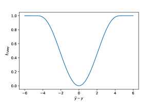
Figure 1: Tukey’s loss defined as $\ell_{\rm Tukey}(\widehat{y},y)\coloneqq\min\left(1-\left[1-(\widehat{y}-y)^{2}/\rho^{2}\right]^{3},1\right)\leq 1$. It has been widely used in the context of robust statistics. The hyper-parameter $\rho>0$ is usually set to $4.685$ for this loss function, and it provides an asymptotic efficiency $95\%$ of that of least squares for Gaussian noise (Andersen, 2008). Here, we rescale the standard Tukey’s bisquare loss for convenience, which does not change the minimizer of the test risk.

Remark 1

The two-step approach that first applies uLSIF to estimate the importance weights and then employs IWERM is equivalent to minimizing the second term of the above upper bounds first and then minimizing the first term, which leads to a sub-optimal solution to the upper-bound minimization.

Instead of estimating the unknown $r(\bm{x})$ for minimizing $R(f)$ as in the previous two-step approaches, we propose a one-step approach that minimizes the upper bound $J(f,g)$ or $J_{\mathrm{UB}}(f,g)$ based on Theorem 3.1.

For classification problems, $J(f,g)$ is defined using the zero-one loss, with which training will not be tractable (Ben-David et al., 2003). Fortunately, the latter part of Theorem 3.1 allows us to minimize $J_{\mathrm{UB}}(f,g)$ instead, with $\ell_{\mathrm{UB}}$ being any (sub-)differentiable approximation that bounds the zero-one loss from above so that we can apply any gradient method such as stochastic gradient descent (Robbins and Monro, 1951). Examples of such $\ell_{\mathrm{UB}}$ include the hinge loss $\ell(\widehat{y},y)=\operatorname{max}(0,1-\widehat{y}y)$ and the squared loss. For regression problems, Tukey’s loss is already differentiable, but we can use the squared loss that bounds Tukey’s loss which makes the optimization problem simpler as described later. This is again justified by Theorem 3.1 with the squared loss used for the upper-bound loss $\ell_{\mathrm{UB}}$.

Although the second expectation in $J_{\mathrm{UB}}(f,g)$ contains an unknown term $r(\bm{x})$, it can be estimated from the samples on hand, up to addition by a constant due to the fact that

$$\phantom{=\ }\mathbb{E}_{\bm{x}^{\mathrm{tr}}\sim p_{\mathrm{tr}}(\bm{x})}\left[\left(g(\bm{x}^{\mathrm{tr}})-r(\bm{x}^{\mathrm{tr}})\right)^{2}\right]$$

$$=\mathbb{E}_{\bm{x}^{\mathrm{tr}}\sim p_{\mathrm{tr}}(\bm{x})}\left[g^{2}(\bm{x}^{\mathrm{tr}})\right]-2\mathbb{E}_{\bm{x}^{\mathrm{te}}\sim p_{\mathrm{te}}(\bm{x})}\left[g(\bm{x}^{\mathrm{te}})\right]+C,$$

where $C$ is a constant that does not depend on the function $f$ nor $g$.

Since the true distributions are unknown, we minimize its empirical version $\widehat{J}_{\mathrm{UB}}(f,g;S)$ with respect to $f$ and non-negative $g$ in some given hypothesis sets $\mathcal{F}$ and $\mathcal{G}_{+}$:

$$\widehat{J}_{\mathrm{UB}}(f,g;S) \coloneqq\left(\frac{1}{n_{\mathrm{tr}}}\sum_{i=1}^{n_{\mathrm{tr}}}\ell_{\mathrm{UB}}(f(\bm{x}^{\mathrm{tr}}_{i}),y^{\mathrm{tr}}_{i})g(\bm{x}^{\mathrm{tr}}_{i})\right)^{2}$$

$$\phantom{\coloneqq}+m^{2}\left(\frac{1}{n_{\mathrm{tr}}}\sum_{i=1}^{n_{\mathrm{tr}}}g^{2}(\bm{x}^{\mathrm{tr}}_{i})-\frac{2}{n_{\mathrm{te}}}\sum_{i=1}^{n_{\mathrm{te}}}g(\bm{x}^{\mathrm{te}}_{i})+C\right),$$ (4)

where $S\coloneqq\left\{\left(\bm{x}_{i}^{\mathrm{tr}},y_{i}^{\mathrm{tr}}\right)\right\}_{i=1}^{n_{\mathrm{tr}}}\cup\left\{\bm{x}_{i}^{\mathrm{te}}\right\}_{i=1}^{n_{\mathrm{te}}}$ is the set of sample points. Notice that constant $C$ can be safely ignored in the minimization.

Below, we present an alternating minimization algorithm described in Algorithm 1 that can be employed when $f(\bm{x})$ and $g(\bm{x})$ are linear-in-parameter models, i.e.,

$$f(\bm{x})=\bm{\alpha}^{\top}\bm{\phi}(\bm{x})\quad\text{and}\quad g(\bm{x})=\bm{\beta}^{\top}\bm{\psi}(\bm{x}),$$ (5)

where $\bm{\alpha}\in\mathbb{R}^{b_{f}}$ and $\bm{\beta}\in\mathbb{R}^{b_{g}}$ are parameters, and $\bm{\phi}$ and $\bm{\psi}$ are $b_{f}$-dimensional and $b_{g}$-dimensional vectors of basis functions.

First, we minimize the objective (3.1) with respect to $g$ while fixing $f$. This step has an analytic solution as shown in Algorithm 1, Line 6, where $\bm{\Phi}_{\mathrm{tr}}=(\bm{\phi}(\bm{x}^{\mathrm{tr}}_{1}),\ldots,\bm{\phi}(\bm{x}^{\mathrm{tr}}_{n_{\mathrm{tr}}}))^{\top}$, $\bm{\Psi}_{\mathrm{tr}}=(\bm{\psi}(\bm{x}^{\mathrm{tr}}_{1}),\ldots,\bm{\psi}(\bm{x}^{\mathrm{tr}}_{n_{\mathrm{tr}}}))^{\top}$, $\bm{\Psi}_{\mathrm{te}}=(\bm{\psi}(\bm{x}^{\mathrm{te}}_{1}),\ldots,\bm{\psi}(\bm{x}^{\mathrm{te}}_{n_{\mathrm{te}}}))^{\top}$, $\bm{1}=(1,\ldots,1)^{\top}$, and $\bm{I}$ is the identity matrix.

Next, we minimize the objective (3.1) with respect to $f$ while fixing $g$. In this step, we can safely ignore the second term and remove the square operation of the first term in the objective (3.1) to reduce the problem into weighted empirical risk minimization (cf. Algorithm 1, Line 12) by forcing $g$ to be non-negative with a rounding up technique (Kanamori et al., 2009) as shown in Algorithm 1, Line 7. For regression problems, the method of iteratively reweighted least squares (IRLS) (Beaton and Tukey, 1974) can be used for optimizing Tukey’s bisquare loss. In practice, we suggest using the squared loss as a convex approximation of Tukey’s loss to obtain a closed-form solution as shown in Algorithm 1, Line 10 for reducing computation time, and we compare their performance in the experiments. For classification with linear-in-parameter models using the hinge loss, then the weighted support vector machine (Yang et al., 2007) can be used. After this step, we go back to the step for updating $g$ and repeat the procedure.

Algorithm 1 Alternating Minimization with Linear-in-parameter Models

1:  $\bm{\alpha}_{0}\leftarrow$ an arbitrary $b_{f}$-dimensional vector

2:  $\lambda_{g}\leftarrow$ a positive $\ell_{2}$-regularization parameter

3:  $\lambda_{f}\leftarrow$ a positive $\ell_{2}$-regularization parameter

4:  for $t=0,1,\ldots,T-1$ do

5:     $\bm{l}_{t}\leftarrow(\ell_{\mathrm{UB}}(\bm{\alpha}_{t}^{\top}\bm{\phi}(\bm{x}^{\mathrm{tr}}_{1}),y^{\mathrm{tr}}_{1}),\ldots,\ell_{\mathrm{UB}}(\bm{\alpha}_{t}^{\top}\bm{\phi}(\bm{x}^{\mathrm{tr}}_{n_{\mathrm{tr}}}),y^{\mathrm{tr}}_{n_{\mathrm{tr}}}))^{\top}$

6:     $\bm{\beta}_{t+1}\leftarrow\left(\frac{1}{n_{\mathrm{tr}}}\bm{\Psi}_{\mathrm{tr}}^{\top}\bm{\Psi}_{\mathrm{tr}}+\frac{1}{m^{2}n_{\mathrm{tr}}^{2}}\bm{\Psi}_{\mathrm{tr}}^{\top}\bm{l}_{t}\bm{l}_{t}^{\top}\bm{\Psi}_{\mathrm{tr}}+\frac{1}{m^{2}}\lambda_{g}\bm{I}\right)^{-1}\frac{1}{n_{\mathrm{te}}}\bm{\Psi}_{\mathrm{te}}^{\top}\bm{1}$

7:     $\bm{\beta}_{t+1}\leftarrow\max(\bm{\beta}_{t+1},\bm{0})$ 

8:     $w_{i}^{t+1}\leftarrow\bm{\beta}_{t+1}^{\top}\bm{\psi}(\bm{x}_{i}^{\mathrm{tr}})$, $i=1,\ldots,n_{\mathrm{tr}}$

9:     if $\ell_{\mathrm{UB}}$ is the squared loss then

10:        $\bm{\alpha}_{t+1}\leftarrow\left(\bm{\Phi}_{\mathrm{tr}}^{\top}\bm{W}_{t+1}\bm{\Phi}_{\mathrm{tr}}+\lambda_{f}n_{\mathrm{tr}}\bm{I}\right)^{-1}\bm{\Phi}_{\mathrm{tr}}^{\top}\bm{W}_{t+1}\bm{y}_{\mathrm{tr}}$,where $\bm{W}_{t+1}=\operatorname{diag}(w_{1}^{t+1},\ldots,w_{n_{\mathrm{tr}}}^{t+1})$ and $\bm{y}_{\mathrm{tr}}=(y_{1}^{\mathrm{tr}},\ldots,y_{n_{\mathrm{tr}}}^{\mathrm{tr}})^{\top}$

11:     else

12:        $\bm{\alpha}_{t+1}\leftarrow\operatorname*{arg\,min}_{\bm{\alpha}}\frac{1}{n_{\mathrm{tr}}}\sum_{i=1}^{n_{\mathrm{tr}}}w_{i}^{t+1}\ell_{\mathrm{UB}}(\bm{\alpha}_{t}^{\top}\bm{\phi}(\bm{x}^{\mathrm{tr}}_{i}),y^{\mathrm{tr}}_{i})+\lambda_{f}\bm{\alpha}^{\top}\bm{\alpha}$

13:     end if

14:  end for

3.2 Theoretical Analysis

In what follows, we establish a generalization error bound for the proposed method in terms of the Rademacher complexity (Koltchinskii, 2001).

Lemma 1

Assume that (a) there exist some constants $M\geq m$ and $L>0$ such that $\ell_{\mathrm{UB}}(f(\bm{x}),y)\leq M$ holds for every $f\in\mathcal{F}$ and every $(\bm{x},y)\in\mathcal{X}\times\mathcal{Y}$ and $y\mapsto\ell_{\mathrm{UB}}(y,y^{\prime})$ is $L$-Lipschitz for every fixed $y^{\prime}\in\mathcal{Y}$; (b) there exists some constant $G\geq 1$ such that $g(\bm{x})\leq G$ for every $g\in\mathcal{G}_{+}$ and every $\bm{x}\in\mathcal{X}$. Let $\mathcal{G}=\mathcal{G}_{+}\cup-\mathcal{G}_{+}$ Then for any $\delta>0$, with probability at least $1-\delta$ over the draw of $S$, the following holds for all $f\in\mathcal{F},g\in\mathcal{G}_{+}$ uniformly:

$$J_{\mathrm{UB}}(f,g)\leq \widehat{J}_{\mathrm{UB}}(f,g;S)+8MG\left(M+G\right)\left(L\mathfrak{R}^{\mathrm{tr}}_{n_{\mathrm{tr}}}(\mathcal{F})+\mathfrak{R}^{\mathrm{tr}}_{n_{\mathrm{tr}}}(\mathcal{G})\right)$$

$$+4M^{2}\mathfrak{R}^{\mathrm{te}}_{n_{\mathrm{te}}}(\mathcal{G})+5M^{2}G^{2}\sqrt{\frac{\log\frac{1}{\delta}}{2}}\left(\frac{1}{\sqrt{n_{\mathrm{tr}}}}+\frac{1}{\sqrt{n_{\mathrm{te}}}}\right),$$ (6)

where $\mathfrak{R}^{\mathrm{tr}}_{n_{\mathrm{tr}}}(\mathcal{F})$ and $\mathfrak{R}^{\mathrm{tr}}_{n_{\mathrm{tr}}}(\mathcal{G})$ are the Rademacher complexities of $\mathcal{F}$ and $\mathcal{G}$, respectively, for the sampling of size $n_{\mathrm{tr}}$ from $p_{\mathrm{tr}}(\bm{x})$, and $\mathfrak{R}^{\mathrm{te}}_{n_{\mathrm{te}}}(\mathcal{G})$ is the Rademacher complexity of $\mathcal{G}$ for the sampling of size $n_{\mathrm{te}}$ from $p_{\mathrm{te}}(\bm{x})$.

We provide a proof of Lemma 1 in Appendix A. Combining (3.1), (3.1), and (1), we obtain the following theorem.

Theorem 3.2

Suppose that the assumptions in Lemma 1 hold. Then, for any $\delta>0$, with probability at least $1-\delta$ over the draw of $S$, the test risk can be bounded as follows for all $f\in\mathcal{F}$ uniformly:

$$\frac{1}{2}R^{2}(f)\leq \min_{g\in\mathcal{G}_{+}}\widehat{J}_{\mathrm{UB}}(f,g;S)+8MG\left(M+G\right)\left(L\mathfrak{R}^{\mathrm{tr}}_{n_{\mathrm{tr}}}(\mathcal{F})+\mathfrak{R}^{\mathrm{tr}}_{n_{\mathrm{tr}}}(\mathcal{G})\right)$$

$$+4M^{2}\mathfrak{R}^{\mathrm{te}}_{n_{\mathrm{te}}}(\mathcal{G})+5M^{2}G^{2}\sqrt{\frac{\log\frac{1}{\delta}}{2}}\left(\frac{1}{\sqrt{n_{\mathrm{tr}}}}+\frac{1}{\sqrt{n_{\mathrm{te}}}}\right).$$ (7)

Theorem 3.2 implies that minimizing $\widehat{J}_{\mathrm{UB}}(f,g;S)$, as the proposed method does, amounts to minimizing an upper bound of the test risk. Furthermore, the following theorem shows a generalization error bound for the minimizer obtained by the proposed method.

Theorem 3.3

Let $(\widehat{f},\widehat{g})=\operatorname*{arg\,min}_{(f,g)\in\mathcal{F}\times\mathcal{G}_{+}}\widehat{J}_{\mathrm{UB}}(f,g;S)$. Then, under the assumptions of Lemma 1, for any $\delta>0$, it holds with probability at least $1-\delta$ over the draw of $S$ that

$$\frac{1}{2}R^{2}(\widehat{f})\leq \min_{f\in\mathcal{F},g\in\mathcal{G}_{+}}J_{\mathrm{UB}}(f,g)+8MG\left(M+G\right)\left(L\mathfrak{R}^{\mathrm{tr}}_{n_{\mathrm{tr}}}(\mathcal{F})+\mathfrak{R}^{\mathrm{tr}}_{n_{\mathrm{tr}}}(\mathcal{G})\right)$$

$$+4M^{2}\mathfrak{R}^{\mathrm{te}}_{n_{\mathrm{te}}}(\mathcal{G})+10M^{2}G^{2}\sqrt{\frac{\log\frac{1}{\delta}}{2}}\left(\frac{1}{\sqrt{n_{\mathrm{tr}}}}+\frac{1}{\sqrt{n_{\mathrm{te}}}}\right)+\frac{M^{2}G^{2}}{n_{\mathrm{tr}}}.$$ (8)

A proof of Theorem 3.3 is presented in Appendix B. If we use linear-in-parameter models with bounded norms, then $\mathfrak{R}^{\mathrm{tr}}_{n_{\mathrm{tr}}}(\mathcal{F})=O(1/\sqrt{n_{\mathrm{tr}}})$, $\mathfrak{R}^{\mathrm{tr}}_{n_{\mathrm{tr}}}(\mathcal{G})=O(1/\sqrt{n_{\mathrm{tr}}})$, and $\mathfrak{R}^{\mathrm{te}}_{n_{\mathrm{te}}}(\mathcal{G})=O(1/\sqrt{n_{\mathrm{te}}})$ (Mohri et al., 2018; Shalev-Shwartz and Ben-David, 2014). Furthermore, if we assume that the approximation error of $\mathcal{G}_{+}$ is zero, i.e., $r\in\mathcal{G}_{+}$, then $\min_{f\in\mathcal{F},g\in\mathcal{G}+}J_{\mathrm{UB}}(f,g)\leq J_{\mathrm{UB}}(f^{*},r)=R_{\mathrm{UB}}^{2}(f^{*})$, where $R_{\mathrm{UB}}$ is the test risk defined with $\ell_{\mathrm{UB}}$ and $f^{*}=\operatorname*{arg\,min}_{f\in\mathcal{F}}R_{\mathrm{UB}}(f)$. Thus,

$$R(\widehat{f})\leq\sqrt{2}R_{\mathrm{UB}}(f^{*})+O_{p}(1/\sqrt[4]{n_{\mathrm{tr}}}+1/\sqrt[4]{n_{\mathrm{te}}}).$$

When the best-in-class test risk $R_{\mathrm{UB}}(f^{*})$ is small, this bound would theoretically guarantee a good performance of the proposed method.

4 Experiments on Regression and Binary Classification

In this section, we examine the effectiveness of the proposed method via experiments on toy regression and binary classification benchmark datasets.

4.1 Illustration with Toy Regression Datasets

First, we conduct experiments on a toy regression dataset.

Let us consider a one-dimensional regression problem. Let the training and test input densities be

$$p_{\mathrm{tr}}(x)=N(x;1,(0.5)^{2})\text{\quad and \quad}p_{\mathrm{te}}(x)=N(x;2,(0.25)^{2}),$$

where $N(x;\mu,\sigma^{2})$ denotes the Gaussian density with mean $\mu$ and variance $\sigma^{2}$. Consider the case where the output labels of examples are generated by

$$y=f^{*}(x)+\epsilon\quad\text{with}\quad f^{*}(x)=\operatorname{sinc}(x),$$

and the noise $\epsilon$ following $N\left(0,(0.1)^{2}\right)$ is independent of $x$. As illustrated in Fig. 2, the training input points are distributed on the left-hand side of the input domain and the test input points are distributed on the right-hand side. We sample $n_{\mathrm{tr}}=150$ labeled i.i.d. training samples $\left\{\left(x_{i}^{\mathrm{tr}},y_{i}^{\mathrm{tr}}\right)\right\}_{i=1}^{n_{\mathrm{tr}}}$ with each $x_{i}^{\mathrm{tr}}$ following $p_{\mathrm{tr}}(x)$ and $n_{\mathrm{te}}=150$ unlabeled i.i.d. test samples $\{x_{i}^{\mathrm{te}}\}_{i=1}^{n_{\mathrm{te}}}$ following $p_{\mathrm{te}}(x)$ for learning the target function $f^{*}(x)$ in the experiment. In addition, we sample 10000 labeled i.i.d. test samples $\left\{(x_{i}^{\mathrm{eval}},y_{i}^{\mathrm{eval}})\right\}_{i=1}^{n_{\mathrm{eval}}}$ with each $(x_{i}^{\mathrm{eval}},y_{i}^{\mathrm{eval}})$ following $p_{\mathrm{te}}(x,y)$ for evaluating the performance of learned functions.

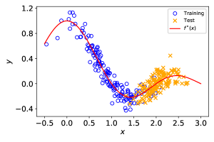
Figure 2: A toy regression example. The training input points (blue) are distributed on the left-hand side of the input domain and the test input points (orange) are distributed on the right-hand side. The two distributions share the same regression function $f^{*}$ (the red curve).

We compare our one-step approach with three baseline methods, which are the ordinary ERM, EIWERM with uLSIF, and RIWERM. We use the linear-in-parameter models (5) with the following Gaussian kernels as basis functions for learning the input-output relation and the importance (or the relative importance) in all the experiments including those in Section 4.2:

$$\phi_{i}(\bm{x})=\exp\bigg{\{}-\frac{\|\bm{x}-\bm{c}^{f}_{i}\|^{2}}{2\sigma_{f}^{2}}\bigg{\}}\quad\text{and}\quad\psi_{i}(\bm{x})=\exp\bigg{\{}-\frac{\|\bm{x}-\bm{c}^{g}_{i}\|^{2}}{2\sigma_{g}^{2}}\bigg{\}},$$

where $\sigma_{f}$ and $\sigma_{g}$ are the bandwidths of the Gaussian kernels, and $\bm{c}_{i}^{f}$ and $\bm{c}_{i}^{g}$ are the kernel centers randomly chosen from $\{\bm{x}_{i}^{\mathrm{te}}\}_{i=1}^{n_{\mathrm{te}}}$ (Kanamori et al., 2009; Sugiyama et al., 2008). We set $b_{f}=b_{g}=50$ in all the experiments. Moreover, we use $\ell_{2}$ regularization in all the experiments, which introduces two more hyperparameters $\lambda_{f}$ and $\lambda_{g}$ associated with models $f$ and $g$ respectively.

Let us clarify the hyperparameter tuning procedure for each method. For the ordinary ERM, the standard cross validation is applied for tuning $\sigma_{f}$ and $\lambda_{f}$. For the EIWERM with uLSIF, the hyperparameter tuning of $\sigma_{g}$ and $\lambda_{g}$ in the importance estimation step uses the cross validation naturally based on its learning objective (cf. Kanamori et al. (2009)), and we apply IWCV in the training step for selecting $\sigma_{f}$, $\lambda_{f}$ and flattening parameter $\gamma$. For RIWERM, the built-in cross validation with its learning objective is used for tuning $\sigma_{g}$ and $\lambda_{g}$ (cf. Yamada et al. (2011)), and the selection of $\sigma_{f}$, $\lambda_{f}$ and parameter $\alpha$ in the training step is achieved by IWCV (the importance is obtained by uLSIF). Finally, for our one-step approach, we can naturally perform cross validation based on the proposed learning objective (3.1). Since all the hyperparameters are tuned simultaneously in the one-step approach, it is computationally expensive as shown in Table 1. To make the one-step approach computationally more efficient, we suggest two heuristics to predetermine some of the hyperparameters. The first one is to set the bandwidths to the median distances between samples and kernel centers, which is a popular heuristic in practice (Schölkopf and Smola, 2001), and we tune the regularization parameters by cross validation. For a fair comparison, we also report the results of the baseline methods using the median heuristic. The second one is to use the hyperparameters of model $g$ determined by uLSIF and tune the hyperparameters of model $f$ by cross validation, since the one-step approach has a close relationship with uLSIF.

As suggested in Section 3.1, we use the squared loss in the one-step approach for computational efficiency. We also employ the IRLS algorithm for optimizing Tukey’s bisquare loss in the one-step approach. For better comparison, we report the results of the baseline methods using both the squared loss and Tukey’s bisquare loss.

The experimental results of the toy regression problem are summarized in Table 1. Note that when the target function $f^{*}$ is perfectly learned, the mean squared error is the variance of $\epsilon$, i.e., 0.01. Therefore, our method significantly mitigates the influence of covariate shift. Since the IRLS algorithm is needed when using Tukey’s bisquare loss, the training should take longer time than that when using the squared loss, and we confirm it according to the results in Table 1.

Table 1: Mean squared test errors averaged over 100 trials on the toy dataset. The numbers in the brackets are the standard deviations. The best method and comparable ones based on the paired t-test at the significance level 5% are described in bold face. The computation time is averaged over 100 trials. “Squared” denotes the squared loss, “Tukey” denotes Tukey’s bisquare loss, “median” means that the bandwidths of the kernel models are determined by the median heuristic (other hyperparameters are still chosen by cross validation), and “uLSIF” means that the hyperparameters of model $g$ are the same as those used in uLSIF (the hyperparameters of model $f$ are still chosen by cross validation).

Methods	MSE(SD)	Computation time (sec)
ERM (squared)	0.0517 (0.0300)	0.25
EIWERM (squared)	0.0265 (0.0361)	2.71
RIWERM (squared)	0.0265 (0.0405)	3.90
one-step (squared)	0.0173 (0.0107)	64.68
one-step (squared, uLSIF)	0.0173 (0.0107)	0.87
ERM (Tukey)	0.0511 (0.0455)	0.62
EIWERM (Tukey)	0.0248 (0.0430)	6.03
RIWERM (Tukey)	0.0227 (0.0223)	7.17
one-step (Tukey)	0.0163 (0.0093)	134.16
one-step (Tukey, uLSIF)	0.0163 (0.0093)	1.66
ERM (squared, median)	0.1453 (0.1812)	0.04
EIWERM (squared, median)	0.0198 (0.0151)	0.33
RIWERM (squared, median)	0.0162 (0.0100)	0.47
one-step (squared, median)	0.0131 (0.0036)	0.73
ERM (Tukey, median)	0.0760 (0.0733)	0.09
EIWERM (Tukey, median)	0.0161 (0.0106)	0.76
RIWERM (Tukey, median)	0.0149 (0.0073)	0.84
one-step (Tukey, median)	0.0125 (0.0021)	1.50

4.2 Experiments on Regression and Binary Classification Benchmark Datasets

Below, we conduct experiments on regression benchmark datasets from UCI and binary classification benchmark datasets from LIBSVM.

We consider experimental settings with both synthetically created covariate shift and naturally occurring covariate shift. To perform train-test split for the datasets with naturally occurring covariate shift, we follow Ahmed et al. (2014), Chen et al. (2016), and Storkey and Sugiyama (2007) to separate the auto mpg dataset, the bike sharing dataset, the parkinsons dataset, and the wine quality dataset based on different origins, different semesters, different age ranges, and different types, respectively. In the rest of the datasets, we synthetically introduce covariate shift in the following way similarly to Cortes et al. (2008). First, we use Z-score normalization to preprocess all the input samples. Then, an example $(\bm{x},y)$ is assigned to the training dataset with probability $\exp(v)/(1+\exp(v))$ and to the test dataset with probability $1/(1+\exp(v))$, where $v=16\bm{w}^{\top}\bm{x}/\sigma$, $\sigma$ is the standard deviation of $\bm{w}^{\top}\bm{x}$, and $\bm{w}\in\mathbb{R}^{d}$ is some given projection vector. To ensure that the methods are tested in challenging covariate shift situations, we randomly sample projection directions and choose the one such that the classifier trained on the training dataset generalizes worst to the test dataset for train-test split.

By following the above procedure, we split the datasets into training datasets and test datasets (with some randomness in synthetic cases). Then we sample a certain number (depending on the size of the dataset) of training samples and test input samples for training. We use the rest of test samples for evaluating the performance. We run 100 trials for each dataset.

The models and the hyperparameter tuning procedure follow what we discussed in Section 4.1. To reduce computation time, we employ the two heuristics mentioned in Section 4.1 for the one-step approach. In addition, as discussed in Section 3.1, we use the squared loss as the surrogate loss function for all the methods including the one-step approach in the experiments.

The experimental results on benchmark datasets are summarized in Table 2. The table shows the proposed one-step approach outperforms or is comparable to the baseline methods with the best performance, which suggests that it is a promising method for covariate shift adaptation.

Table 2: Mean squared test errors/mean test misclassification rates averaged over 100 trials on regression/binary classification benchmark datasets. The numbers in the brackets are the standard deviations. All the error values are normalized so that the mean error by “ERM” will be one. For each dataset, the best method and comparable ones based on the paired t-test at the significance level 5% are described in bold face. The upper half are regression datasets and the lower half are binary classification datasets.

Dataset	ERM	ERM (median)	EIWERM	EIWERM (median)	RIWERM	RIWERM (median)	one-step (uLSIF)	one-step (median)
auto	1.00 (0.22)	1.22 (0.29)	1.09 (0.25)	1.08 (0.25)	1.09 (0.26)	1.08 (0.23)	1.00 (0.26)	0.99 (0.21)
bike	1.00 (0.10)	0.97 (0.10)	1.05 (0.19)	0.97 (0.10)	1.02 (0.13)	0.98 (0.10)	1.05 (0.15)	0.95 (0.08)
parkinsons	1.00 (0.28)	0.94 (0.22)	1.05 (0.37)	0.93 (0.17)	1.02 (0.37)	0.92 (0.16)	0.78 (0.07)	0.76 (0.05)
wine	1.00 (0.22)	0.95 (0.13)	1.05 (0.24)	0.95 (0.12)	1.07 (0.36)	0.95 (0.14)	0.96 (0.10)	0.90 (0.07)
australian	32.02 (16.88)	31.62 (17.88)	30.70 (16.35)	31.00 (17.47)	29.82 (14.83)	31.81 (17.52)	28.45 (13.86)	25.57 (12.74)
breast	22.72 (13.12)	22.13 (10.36)	21.84 (13.16)	21.82 (11.20)	23.58 (12.57)	22.00 (13.38)	16.55 (9.09)	22.51 (12.56)
diabetes	45.78 (8.88)	43.35 (9.56)	42.44 (7.65)	41.67 (8.66)	43.26 (8.42)	44.65 (10.07)	39.58 (5.29)	38.57 (6.36)
heart	36.39 (11.90)	34.91 (12.45)	32.06 (11.05)	35.13 (12.57)	33.39 (12.24)	35.77 (15.26)	31.39 (10.36)	31.88 (11.95)
sonar	39.57 (7.10)	39.03 (6.69)	39.19 (7.00)	38.77 (6.37)	38.83 (7.15)	39.03 (6.39)	37.69 (7.17)	39.23 (7.17)

5 Extension to Multi-class Classification with Neural Networks

In this section, we extend the proposed method to multi-class classification and conduct experiments with neural networks.

Consider a $K$-class classification problem with an input space $\mathcal{X}\subset\mathbb{R}^{d}$ and an output space $\mathcal{Y}=\{1,\ldots,K\}$, and let $\bm{f}\colon\mathcal{X}\rightarrow\mathbb{R}^{K}$ be the classifier to be trained for this problem and $\ell\colon\mathbb{R}^{K}\times\mathcal{Y}\to\mathbb{R}_{+}$ be the loss function in the test risk $R(\bm{f})$ (cf. Eq. (1)). The zero-one loss $\ell(\bm{o},y)=I(y\neq\operatorname*{arg\,max}_{k\in\mathcal{Y}}\bm{o}_{k})$ is a typical choice, where $\bm{o}\in\mathbb{R}^{K}$ and $\bm{o}_{k}$ denotes the $k$-th element of $\bm{o}$. As discussed in Section 3.1, we can use a surrogate loss $\ell_{\mathrm{UB}}$ that bounds the zero-one loss from above, e.g., the softmax cross-entropy loss, to obtain a tractable upper-bound $J_{\mathrm{UB}}(\bm{f},g)$ (cf. Eq. (3.1)). We present a gradient-based alternating minimization algorithm described in Algorithm 2 that is more convenient for training neural networks.

Algorithm 2 Gradient-based Alternating Minimization

1:  $\mathcal{Z}^{\mathrm{tr}},\mathcal{X}^{\mathrm{te}}\leftarrow\left\{\left(\bm{x}_{i}^{\mathrm{tr}},y_{i}^{\mathrm{tr}}\right)\right\}_{i=1}^{n_{\mathrm{tr}}},\left\{\bm{x}_{i}^{\mathrm{te}}\right\}_{i=1}^{n_{\mathrm{te}}}$

2:  $\mathcal{A}\leftarrow$ a gradient-based optimizer

3:  $\bm{f}\leftarrow$ an arbitrary classifier

4:  for $\mathrm{round}=0,1,\ldots,\mathrm{numOfRounds}-1$ do

5:     for $\mathrm{epoch}=0,1,\ldots,\mathrm{numOfEpochsForG}-1$ do

6:        for $i=0,1,\ldots,\mathrm{numOfMiniBatches}-1$ do

7:           $\mathcal{Z}_{i}^{\mathrm{tr}},\mathcal{X}_{i}^{\mathrm{te}}\leftarrow\mathrm{sampleMiniBatch}(\mathcal{Z}^{\mathrm{tr}},\mathcal{X}^{\mathrm{te}})$

8:           $g\leftarrow\mathcal{A}(g,\nabla_{g}\widehat{J}_{\mathrm{UB}}(\bm{f},g;\mathcal{Z}_{i}^{\mathrm{tr}}\cup\mathcal{X}_{i}^{\mathrm{te}}))$

9:        end for

10:     end for

11:     for $\mathrm{epoch}=0,1,\ldots,\mathrm{numOfEpochsForF}-1$ do

12:        for $i=0,1,\ldots,\mathrm{numOfMiniBatches}-1$ do

13:           $\mathcal{Z}_{i}^{\mathrm{tr}}\leftarrow\mathrm{sampleMiniBatch}(\mathcal{Z}^{\mathrm{tr}})$

14:           $w_{j}\leftarrow\max(g(\bm{x}_{j}),0)$, $\forall(\bm{x}_{j},\cdot)\in\mathcal{Z}_{i}^{\mathrm{tr}}$

15:           $w_{j}\leftarrow w_{j}/\sum_{j}w_{j}$, $\forall j$

16:           $L_{i}\leftarrow\sum_{(\bm{x}_{j},y_{j})\in\mathcal{Z}_{i}^{\mathrm{tr}}}w_{j}\ell_{\mathrm{UB}}(\bm{f}(\bm{x}_{j}),y_{j})$

17:           $\bm{f}\leftarrow\mathcal{A}(\bm{f},\nabla_{\bm{f}}L_{i})$

18:        end for

19:     end for

20:  end for

Below, we design a covariate shift setting and conduct experiments on the Fashion-MNIST (Xiao et al., 2017) and Kuzushiji-MNIST (Clanuwat et al., 2018) benchmark datasets for image classification using convolutional neural networks (CNNs).

Based on the fact that the labels of the images from those datasets are invariant to rotation transformation, we introduce covariate shift to the image datasets in the following way: we rotate each image $I_{i}$ in the training sets by angle $\theta_{i}$, where $\theta_{i}/180^{\circ}$ is drawn from a Beta distribution $\mathrm{Beta}(a,b)$, and rotate each image $J_{i}$ in the test sets by angle $\phi_{i}$, where $\phi_{i}/180^{\circ}$ is drawn from another Beta distribution $\mathrm{Beta}(b,a)$. The parameters $a$ and $b$ control the shift level, and we test three different levels in our experiments: $(a,b)=(2,4)$, $(2,5)$, and $(2,6)$. Since our experiments are conducted in an inductive manner, we also rotate each image $I_{i}$ in the training sets by angle $\psi_{i}$, where $\psi_{i}/180^{\circ}$ is drawn from the Beta distribution $\mathrm{Beta}(b,a)$ to obtain the unlabeled test images for training.

We compare our one-step approach with three baseline methods: the ordinary ERM, EIWERM with $\gamma=0.5$, and RIWERM with $\alpha=0.5$. We use the softmax cross-entropy loss as a surrogate loss and use 5-layer CNNs, which consist of 2 convolutional layers with pooling and 3 fully connected layers, to model the classifier $\bm{f}$ and the weight model $g$. In order to learn useful weights, we pretrain $g$ in a binary classification problem whose goal is to discriminate between $\left\{\bm{x}_{i}^{\mathrm{tr}}\right\}_{i=1}^{n_{\mathrm{tr}}}$ and $\left\{\bm{x}_{i}^{\mathrm{te}}\right\}_{i=1}^{n_{\mathrm{te}}}$ and freeze the parameters in the first two convolutional layers. We train $\bm{f}$ and $g$ for 20 rounds for the one-step approach, where a round consists of 5 epochs of training $g$ followed by 10 epochs of training $\bm{f}$: we train the models for 300 epochs in total. We use stochastic gradient descent with a learning rate of $10^{-4}$ and mini-batch size of 128 for training $g$ and use Adam (Kingma and Ba, 2015) with an initial learning rate of $10^{-3}$ halved every 4 rounds and mini-batch size of 128 for training $\bm{f}$. For a fair comparison, we train the (relative) importance models for 100 epochs and the classifiers for 200 epochs in the baseline methods.

The experimental results summarized in Table 3 verify the effectiveness of our one-step approach in image classification problems with neural networks. Specifically, the table shows that the ordinary ERM performs poorly under covariate shift, the weighted methods all improve the performance, and the one-step approach further improves the performance especially under large covariate shift (i.e., the difference between shift parameters $a$ and $b$ is large).

Table 3: Mean test classification accuracy averaged over 5 trials on image datasets with neural networks. The numbers in the brackets are the standard deviations. For each dataset, the best method and comparable ones based on the paired t-test at the significance level 5% are described in bold face.

Dataset	Shift Level ($a$, $b$)	ERM	EIWERM	RIWERM	one-step
	(2, 4)	81.71(0.17)	84.02(0.18)	84.12(0.06)	85.07(0.08)
Fashion-MNIST	(2, 5)	72.52(0.54)	76.68(0.27)	77.43(0.29)	78.83(0.20)
	(2, 6)	60.10(0.34)	65.73(0.34)	66.73(0.55)	69.23(0.25)
	(2, 4)	77.09(0.18)	80.92(0.32)	81.17(0.24)	82.45(0.12)
Kuzushiji-MNIST	(2, 5)	65.06(0.26)	71.02(0.50)	72.16(0.19)	74.03(0.16)
	(2, 6)	51.24(0.30)	58.78(0.38)	60.14(0.93)	62.70(0.55)

6 Conclusion

In this work, we studied the problem of covariate shift adaptation. Unlike the dominating two-step approaches in the literature, we proposed a one-step approach that learns the predictive model and the associated weights simultaneously by following Vapnik’s principle. Our experiments highlighted the advantage of our method over previous two-step approaches, suggesting that the proposed one-step approach is a promising method for covariate shift adaptation. For future work, it would be interesting to investigate whether the proposed method is still useful in covariate shift adaptation for nowadays prevalent extremely deep neural networks because importance weighting is valid only when the model used for learning is misspecified (Sugiyama and Kawanabe, 2012).

Appendix A Proof of Lemma 1

Proof

Let $\Phi(S)=\sup_{f\in\mathcal{F},g\in\mathcal{G}_{+}}\left(J_{\mathrm{UB}}(f,g)-\widehat{J}_{\mathrm{UB}}(f,g;S)\right)$ and $S^{\prime}$ be a set differing from $S$ on exactly one sample point. Then, since the difference of suprema does not exceed the supremum of the difference, we have

$$\Phi(S^{\prime})-\Phi(S)\leq\sup_{f\in\mathcal{F},g\in\mathcal{G}_{+}}\left(\widehat{J}_{\mathrm{UB}}(f,g;S)-\widehat{J}_{\mathrm{UB}}(f,g;S^{\prime})\right).$$

If the differing sample point is a training sample, then

$$\Phi(S^{\prime})-\Phi(S)\leq 2MG\cdot\frac{2}{n_{\mathrm{tr}}}MG+M^{2}\cdot\frac{1}{n_{\mathrm{tr}}}G^{2}=\frac{5}{n_{\mathrm{tr}}}M^{2}G^{2}.$$

On the other hand, if the differing sample point is a test sample, then

$$\Phi(S^{\prime})-\Phi(S)\leq M^{2}\cdot\frac{2}{n_{\mathrm{te}}}\cdot 2G\leq\frac{5}{n_{\mathrm{te}}}M^{2}G^{2}.$$

Similarly, we can obtain the same result for bounding $\Phi(S)-\Phi(S^{\prime})$. Then, by McDiarmid’s inequality, for any $\delta>0$, with probability at least $1-\delta$, the following holds:

$$\Phi(S)\leq\mathbb{E}_{S}[\Phi(S)]+5M^{2}G^{2}\sqrt{\frac{\log\frac{1}{\delta}}{2}}\left(\frac{1}{\sqrt{n_{\mathrm{tr}}}}+\frac{1}{\sqrt{n_{\mathrm{te}}}}\right).$$

Let $S_{\mathrm{tr}}=\left\{\left(\bm{x}_{i}^{\mathrm{tr}},y_{i}^{\mathrm{tr}}\right)\right\}_{i=1}^{n_{\mathrm{tr}}}$ and $S_{\mathrm{te}}=\left\{\bm{x}_{i}^{\mathrm{te}}\right\}_{i=1}^{n_{\mathrm{te}}}$. We next bound the expectation in the right-hand side:

$$\mathbb{E}_{S}[\Phi(S)] =\mathbb{E}_{S}\left[\sup_{f\in\mathcal{F},g\in\mathcal{G}_{+}}\left(J_{\mathrm{UB}}(f,g)-\widehat{J}_{\mathrm{UB}}(f,g;S)\right)\right]\leq({\rm I})+M^{2}({\rm II})+2M^{2}({\rm III}),$$

where

$$({\rm I}) =\mathbb{E}_{S_{\mathrm{tr}}}\Bigg{[}\sup_{f\in\mathcal{F},g\in\mathcal{G}_{+}}\Bigg{(}\left(\mathbb{E}_{(\bm{x}^{\mathrm{tr}},y^{\mathrm{tr}})}\left[\ell_{\mathrm{UB}}(f(\bm{x}^{\mathrm{tr}}),y^{\mathrm{tr}})g(\bm{x}^{\mathrm{tr}})\right]\right)^{2}$$

$$\phantom{=\mathbb{E}_{S_{\mathrm{tr}}}\Bigg{[}\sup_{f\in\mathcal{F},g\in\mathcal{G}_{+}}\Bigg{(}(}-\left(\frac{1}{n_{\mathrm{tr}}}\sum_{i=1}^{n_{\mathrm{tr}}}\ell_{\mathrm{UB}}(f(\bm{x}^{\mathrm{tr}}_{i}),y^{\mathrm{tr}}_{i})g(\bm{x}^{\mathrm{tr}}_{i})\right)^{2}\Bigg{)}\Bigg{]},$$

$$({\rm II}) =\mathbb{E}_{S_{\mathrm{tr}}}\left[\sup_{g\in\mathcal{G}_{+}}\left(\mathbb{E}_{\bm{x}^{\mathrm{tr}}}\left[g^{2}(\bm{x}^{\mathrm{tr}})\right]-\frac{1}{n_{\mathrm{tr}}}\sum_{i=1}^{n_{\mathrm{tr}}}g^{2}(\bm{x}^{\mathrm{tr}}_{i})\right)\right],$$

$$({\rm III}) =\mathbb{E}_{S_{\mathrm{te}}}\left[\sup_{g\in\mathcal{G}_{+}}\left(\frac{1}{n_{\mathrm{te}}}\sum_{i=1}^{n_{\mathrm{te}}}g(\bm{x}^{\mathrm{te}}_{i})-\mathbb{E}_{\bm{x}^{\mathrm{te}}\sim p_{\mathrm{te}}(\bm{x})}\left[g(\bm{x}^{\mathrm{te}})\right]\right)\right].$$

Then we bound the above three terms as follows:

$$({\rm I}) \leq\mathbb{E}_{S_{\mathrm{tr}}}\Bigg{[}\sup_{f\in\mathcal{F},g\in\mathcal{G}_{+}}\Bigg{(}\mathbb{E}_{\tilde{S}_{\mathrm{tr}}}\left(\frac{1}{n_{\mathrm{tr}}}\sum_{i=1}^{n_{\mathrm{tr}}}\ell_{\mathrm{UB}}(f(\tilde{\bm{x}}^{\mathrm{tr}}_{i}),\tilde{y}^{\mathrm{tr}}_{i})g(\tilde{\bm{x}}^{\mathrm{tr}}_{i})\right)^{2}$$

$$\phantom{\leq\mathbb{E}_{S_{\mathrm{tr}}}\Bigg{[}\sup_{f\in\mathcal{F},g\in\mathcal{G}_{+}}\Bigg{(}}-\left(\frac{1}{n_{\mathrm{tr}}}\sum_{i=1}^{n_{\mathrm{tr}}}\ell_{\mathrm{UB}}(f(\bm{x}^{\mathrm{tr}}_{i}),y^{\mathrm{tr}}_{i})g(\bm{x}^{\mathrm{tr}}_{i})\right)^{2}\Bigg{)}\Bigg{]}$$

   (points in $$\tilde{S}_{\mathrm{tr}} p_{\mathrm{tr}}(\bm{x},y)$$ are sampled in an i.i.d. fashion from )

$$\leq\mathbb{E}_{S_{\mathrm{tr}},\tilde{S}_{\mathrm{tr}}}\Bigg{[}\sup_{f\in\mathcal{F},g\in\mathcal{G}_{+}}\Bigg{(}\left(\frac{1}{n_{\mathrm{tr}}}\sum_{i=1}^{n_{\mathrm{tr}}}\ell_{\mathrm{UB}}(f(\tilde{\bm{x}}^{\mathrm{tr}}_{i}),\tilde{y}^{\mathrm{tr}}_{i})g(\tilde{\bm{x}}^{\mathrm{tr}}_{i})\right)^{2}$$

$$\phantom{\leq\mathbb{E}_{S_{\mathrm{tr}},\tilde{S}_{\mathrm{tr}}}\Bigg{[}\sup_{f\in\mathcal{F},g\in\mathcal{G}_{+}}\Bigg{(}}-\left(\frac{1}{n_{\mathrm{tr}}}\sum_{i=1}^{n_{\mathrm{tr}}}\ell_{\mathrm{UB}}(f(\bm{x}^{\mathrm{tr}}_{i}),y^{\mathrm{tr}}_{i})g(\bm{x}^{\mathrm{tr}}_{i})\right)^{2}\Bigg{)}\Bigg{]}$$

$$\leq\mathbb{E}_{S_{\mathrm{tr}},\tilde{S}_{\mathrm{tr}}}\Bigg{[}\sup_{f\in\mathcal{F},g\in\mathcal{G}_{+}}\frac{2MG}{n_{\mathrm{tr}}}\Bigg{|}\sum_{i=1}^{n_{\mathrm{tr}}}\big{(}\ell_{\mathrm{UB}}(f(\tilde{\bm{x}}^{\mathrm{tr}}_{i}),\tilde{y}^{\mathrm{tr}}_{i})g(\tilde{\bm{x}}^{\mathrm{tr}}_{i})$$

$$\phantom{\leq\mathbb{E}_{S_{\mathrm{tr}},\tilde{S}_{\mathrm{tr}}}\Bigg{[}\sup_{f\in\mathcal{F},g\in\mathcal{G}_{+}}\frac{2MG}{n_{\mathrm{tr}}}\Bigg{|}\sum_{i=1}^{n_{\mathrm{tr}}}\big{(}}-\ell_{\mathrm{UB}}(f(\bm{x}^{\mathrm{tr}}_{i}),y^{\mathrm{tr}}_{i})g(\bm{x}^{\mathrm{tr}}_{i})\big{)}\Bigg{|}\Bigg{]}$$

$$=\mathbb{E}_{\bm{\sigma},S_{\mathrm{tr}},\tilde{S}_{\mathrm{tr}}}\Bigg{[}\sup_{f\in\mathcal{F},g\in\mathcal{G}_{+}}\frac{2MG}{n_{\mathrm{tr}}}\Bigg{|}\sum_{i=1}^{n_{\mathrm{tr}}}\sigma_{i}\big{(}\ell_{\mathrm{UB}}(f(\tilde{\bm{x}}^{\mathrm{tr}}_{i}),\tilde{y}^{\mathrm{tr}}_{i})g(\tilde{\bm{x}}^{\mathrm{tr}}_{i})$$

$$\phantom{=\mathbb{E}_{\bm{\sigma},S_{\mathrm{tr}},\tilde{S}_{\mathrm{tr}}}\Bigg{[}\sup_{f\in\mathcal{F},g\in\mathcal{G}_{+}}\frac{2MG}{n_{\mathrm{tr}}}\Bigg{|}\sum_{i=1}^{n_{\mathrm{tr}}}\sigma_{i}\big{(}}-\ell_{\mathrm{UB}}(f(\bm{x}^{\mathrm{tr}}_{i}),y^{\mathrm{tr}}_{i})g(\bm{x}^{\mathrm{tr}}_{i})\big{)}\Bigg{|}\Bigg{]}$$

   ($$\{\sigma_{i}\}_{i=1}^{n_{\mathrm{tr}}}$$ is a Rademacher sequence)

$$\leq 4MG\mathbb{E}_{\bm{\sigma},S_{\mathrm{tr}}}\left[\sup_{f\in\mathcal{F},g\in\mathcal{G}_{+}}\left|\frac{1}{n_{\mathrm{tr}}}\sum_{i=1}^{n_{\mathrm{tr}}}\sigma_{i}\ell_{\mathrm{UB}}(f(\bm{x}^{\mathrm{tr}}_{i}),y^{\mathrm{tr}}_{i})g(\bm{x}^{\mathrm{tr}}_{i})\right|\right]$$

$$\leq 4MG\mathbb{E}_{\bm{\sigma},S_{\mathrm{tr}}}\left[\sup_{f\in\mathcal{F},g\in\mathcal{G}}\frac{1}{n_{\mathrm{tr}}}\sum_{i=1}^{n_{\mathrm{tr}}}\sigma_{i}\ell_{\mathrm{UB}}(f(\bm{x}^{\mathrm{tr}}_{i}),y^{\mathrm{tr}}_{i})g(\bm{x}^{\mathrm{tr}}_{i})\right]$$

$$\leq 2MG\Bigg{(}\mathbb{E}_{\bm{\sigma},S_{\mathrm{tr}}}\left[\sup_{f\in\mathcal{F},g\in\mathcal{G}}\frac{1}{n_{\mathrm{tr}}}\sum_{i=1}^{n_{\mathrm{tr}}}\sigma_{i}\left(\ell_{\mathrm{UB}}(f(\bm{x}^{\mathrm{tr}}_{i}),y^{\mathrm{tr}}_{i})+g(\bm{x}^{\mathrm{tr}}_{i})\right)^{2}\right]$$

$$\qquad+\mathbb{E}_{\bm{\sigma},S_{\mathrm{tr}}}\left[\sup_{f\in\mathcal{F}}\frac{1}{n_{\mathrm{tr}}}\sum_{i=1}^{n_{\mathrm{tr}}}\sigma_{i}\ell_{\mathrm{UB}}^{2}(f(\bm{x}^{\mathrm{tr}}_{i}),y^{\mathrm{tr}}_{i})\right]+\mathbb{E}_{\bm{\sigma},S_{\mathrm{tr}}}\left[\sup_{g\in\mathcal{G}}\frac{1}{n_{\mathrm{tr}}}\sum_{i=1}^{n_{\mathrm{tr}}}\sigma_{i}g^{2}(\bm{x}^{\mathrm{tr}}_{i})\right]\Bigg{)}$$

$$\leq 2MG\Bigg{(}2\left(M+G\right)\mathbb{E}_{\bm{\sigma},S_{\mathrm{tr}}}\left[\sup_{f\in\mathcal{F},g\in\mathcal{G}}\frac{1}{n_{\mathrm{tr}}}\sum_{i=1}^{n_{\mathrm{tr}}}\sigma_{i}\left(\ell_{\mathrm{UB}}(f(\bm{x}^{\mathrm{tr}}_{i}),y^{\mathrm{tr}}_{i})+g(\bm{x}^{\mathrm{tr}}_{i})\right)\right]$$

$$\qquad+2M\mathbb{E}_{\bm{\sigma},S_{\mathrm{tr}}}\left[\sup_{f\in\mathcal{F}}\frac{1}{n_{\mathrm{tr}}}\sum_{i=1}^{n_{\mathrm{tr}}}\sigma_{i}\ell_{\mathrm{UB}}(f(\bm{x}^{\mathrm{tr}}_{i}),y^{\mathrm{tr}}_{i})\right]+2G\mathbb{E}_{\bm{\sigma},S_{\mathrm{tr}}}\left[\sup_{g\in\mathcal{G}}\frac{1}{n_{\mathrm{tr}}}\sum_{i=1}^{n_{\mathrm{tr}}}\sigma_{i}g(\bm{x}^{\mathrm{tr}}_{i})\right]\Bigg{)}$$

(Ledoux-Talagrand contraction lemma (Ledoux and Talagrand, 2013))

$$\leq 4MG\left(2M+G\right)L\mathfrak{R}_{n_{\mathrm{tr}}}(\mathcal{F})+4MG\left(M+2G\right)\mathfrak{R}_{n_{\mathrm{tr}}}(\mathcal{G}),$$

(Ledoux-Talagrand contraction lemma)

$$({\rm II}) =\mathbb{E}_{S_{\mathrm{tr}}}\left[\sup_{g\in\mathcal{G}_{+}}\left(\mathbb{E}_{\tilde{S}_{\mathrm{tr}}}\left[\frac{1}{n_{\mathrm{tr}}}\sum_{i=1}^{n_{\mathrm{tr}}}g^{2}(\tilde{\bm{x}}^{\mathrm{tr}}_{i})\right]-\frac{1}{n_{\mathrm{tr}}}\sum_{i=1}^{n_{\mathrm{tr}}}g^{2}(\bm{x}^{\mathrm{tr}}_{i})\right)\right]$$

$$\leq\mathbb{E}_{S_{\mathrm{tr}},\tilde{S}_{\mathrm{tr}}}\left[\sup_{g\in\mathcal{G}_{+}}\frac{1}{n_{\mathrm{tr}}}\sum_{i=1}^{n_{\mathrm{tr}}}\left(g^{2}(\tilde{\bm{x}}^{\mathrm{tr}}_{i})-g^{2}(\bm{x}^{\mathrm{tr}}_{i})\right)\right]$$

$$=\mathbb{E}_{\bm{\sigma},S_{\mathrm{tr}},\tilde{S}_{\mathrm{tr}}}\left[\sup_{g\in\mathcal{G}_{+}}\frac{1}{n_{\mathrm{tr}}}\sum_{i=1}^{n_{\mathrm{tr}}}\sigma_{i}\left(g^{2}(\tilde{\bm{x}}^{\mathrm{tr}}_{i})-g^{2}(\bm{x}^{\mathrm{tr}}_{i})\right)\right]$$

$$\leq 2\mathbb{E}_{\bm{\sigma},S_{\mathrm{tr}}}\left[\sup_{g\in\mathcal{G}_{+}}\frac{1}{n_{\mathrm{tr}}}\sum_{i=1}^{n_{\mathrm{tr}}}\sigma_{i}g^{2}(\bm{x}^{\mathrm{tr}}_{i})\right]$$

$$\leq 4G\mathfrak{R}_{n_{\mathrm{tr}}}(\mathcal{G}),\quad\text{(Ledoux-Talagrand contraction lemma)}$$

$$({\rm III}) =\mathbb{E}_{S_{\mathrm{te}}}\left[\sup_{g\in\mathcal{G}_{+}}\left(\frac{1}{n_{\mathrm{te}}}\sum_{i=1}^{n_{\mathrm{te}}}g(\bm{x}^{\mathrm{te}}_{i})-\mathbb{E}_{\tilde{S}_{\mathrm{te}}}\left[\frac{1}{n_{\mathrm{te}}}\sum_{i=1}^{n_{\mathrm{te}}}g(\tilde{\bm{x}}^{\mathrm{te}}_{i})\right]\right)\right]$$

$$\leq\mathbb{E}_{S_{\mathrm{te}},\tilde{S}_{\mathrm{te}}}\left[\sup_{g\in\mathcal{G}_{+}}\frac{1}{n_{\mathrm{te}}}\sum_{i=1}^{n_{\mathrm{te}}}\left(g(\bm{x}^{\mathrm{te}}_{i})-g(\tilde{\bm{x}}^{\mathrm{te}}_{i})\right)\right]$$

$$=\mathbb{E}_{\bm{\sigma},S_{\mathrm{te}},\tilde{S}_{\mathrm{te}}}\left[\sup_{g\in\mathcal{G}_{+}}\frac{1}{n_{\mathrm{te}}}\sum_{i=1}^{n_{\mathrm{te}}}\sigma_{i}\left(g(\bm{x}^{\mathrm{te}}_{i})-g(\tilde{\bm{x}}^{\mathrm{te}}_{i})\right)\right]$$

$$\leq 2\mathbb{E}_{\bm{\sigma},S_{\mathrm{te}}}\left[\sup_{g\in\mathcal{G}_{+}}\frac{1}{n_{\mathrm{te}}}\sum_{i=1}^{n_{\mathrm{te}}}\sigma_{i}g(\bm{x}^{\mathrm{te}}_{i})\right]\leq 2\mathfrak{R}_{n_{\mathrm{te}}}(\mathcal{G}).$$

By summarizing all the results above, we complete the proof.

Appendix B Proof of Theorem 3.3

Proof

Let $(f^{*}_{J},g^{*}_{J})=\operatorname*{arg\,min}_{(f,g)\in\mathcal{F}\times\mathcal{G}}J_{\mathrm{UB}}(f,g)$. Then for any $\delta>0$, by McDiarmid’s inequality, with probability at least $1-\delta$, we have

$$\widehat{J}_{\mathrm{UB}}(f^{*}_{J},g^{*}_{J};S)\leq\mathbb{E}_{S}[\widehat{J}_{\mathrm{UB}}(f^{*}_{J},g^{*}_{J};S)]+5M^{2}G^{2}\sqrt{\frac{\log\frac{1}{\delta}}{2}}\left(\frac{1}{\sqrt{n_{\mathrm{tr}}}}+\frac{1}{\sqrt{n_{\mathrm{te}}}}\right).$$

Since $\mathbb{E}\left[X^{2}\right]=\left(\mathbb{E}[X]\right)^{2}+{\rm Var}[X]$, we have

$$\mathbb{E}_{S}[\widehat{J}_{\mathrm{UB}}(f^{*}_{J},g^{*}_{J};S)] =J_{\mathrm{UB}}(f^{*}_{J},g^{*}_{J})+\frac{1}{n_{\mathrm{tr}}}{\rm Var}\left[\ell_{\mathrm{UB}}(f(\tilde{\bm{x}}^{\mathrm{tr}}_{1}),\tilde{y}^{\mathrm{tr}}_{1})g(\tilde{\bm{x}}^{\mathrm{tr}}_{1})\right]$$

$$\leq J_{\mathrm{UB}}(f^{*}_{J},g^{*}_{J})+\frac{1}{n_{\mathrm{tr}}}M^{2}G^{2},$$

and thus,

$$\widehat{J}_{\mathrm{UB}}(f^{*}_{J},g^{*}_{J};S)\leq J_{\mathrm{UB}}(f^{*}_{J},g^{*}_{J})+5M^{2}G^{2}\sqrt{\frac{\log\frac{1}{\delta}}{2}}\left(\frac{1}{\sqrt{n_{\mathrm{tr}}}}+\frac{1}{\sqrt{n_{\mathrm{te}}}}\right)+M^{2}G^{2}\frac{1}{n_{\mathrm{tr}}}.$$

Therefore, according to (3.1), (3.1) and (1), we have

$$\quad\ \frac{1}{2}R^{2}(\widehat{f})-J_{\mathrm{UB}}(f^{*}_{J},g^{*}_{J})$$

$$\leq\left(J_{\mathrm{UB}}(\widehat{f},\widehat{g})-\widehat{J}_{\mathrm{UB}}(\widehat{f},\widehat{g};S)\right)+\left(\widehat{J}_{\mathrm{UB}}(\widehat{f},\widehat{g};S)-\widehat{J}_{\mathrm{UB}}(f^{*}_{J},g^{*}_{J};S)\right)$$

$$\phantom{\leq\ }+\left(\widehat{J}_{\mathrm{UB}}(f^{*}_{J},g^{*}_{J};S)-J_{\mathrm{UB}}(f^{*}_{J},g^{*}_{J})\right)$$

$$\leq\Bigg{(}8MG\left(M+G\right)\left(L\mathfrak{R}^{\mathrm{tr}}_{n_{\mathrm{tr}}}(\mathcal{F})+\mathfrak{R}^{\mathrm{tr}}_{n_{\mathrm{tr}}}(\mathcal{G})\right)+4M^{2}\mathfrak{R}^{\mathrm{te}}_{n_{\mathrm{te}}}(\mathcal{G})$$

$$\phantom{\leq\Bigg{(}}+5M^{2}G^{2}\sqrt{\frac{\log\frac{1}{\delta}}{2}}\left(\frac{1}{\sqrt{n_{\mathrm{tr}}}}+\frac{1}{\sqrt{n_{\mathrm{te}}}}\right)\Bigg{)}+0$$

$$\phantom{\leq\ }+\Bigg{(}5M^{2}G^{2}\sqrt{\frac{\log\frac{1}{\delta}}{2}}\left(\frac{1}{\sqrt{n_{\mathrm{tr}}}}+\frac{1}{\sqrt{n_{\mathrm{te}}}}\right)+M^{2}G^{2}\frac{1}{n_{\mathrm{tr}}}\Bigg{)}.$$

Rearranging the equation above, we obtain Eq. (8).

References

Ahmed et al. (2014)
Ahmed CF, Lachiche N, Charnay C, Braud A (2014) Dataset shift in a real-life
dataset. In: ECML-PKDD Workshop LMCE
Andersen (2008)
Andersen R (2008) Modern Methods for Robust Regression, vol 152. SAGE,
DOI https://doi.org/10.4135/9781412985109
Barron (2019)
Barron JT (2019) A general and adaptive robust loss function. In: IEEE/CVF
Conference on Computer Vision and Pattern Recognition, pp 4326–4334,
DOI 10.1109/CVPR.2019.00446
Beaton and Tukey (1974)
Beaton AE, Tukey JW (1974) The fitting of power series, meaning polynomials,
illustrated on band-spectroscopic data. Technometrics 16(2):147–185,
DOI https://doi.org/10.1080/00401706.1974.10489171
Ben-David et al. (2003)
Ben-David S, Eiron N, Longc PM (2003) On the difficulty of approximately
maximizing agreements. Journal of Computer and System Sciences
66(3):496–514, DOI https://doi.org/10.1016/S0022-0000(03)00038-2
Bickel and Scheffer (2007)
Bickel S, Scheffer T (2007) Dirichlet-enhanced spam filtering based on biased
samples. In: Advances in Neural Information Processing Systems, pp 161–168,
DOI https://doi.org/10.7551/mitpress/7503.003.0025
Bishop (1995)
Bishop CM (1995) Neural Networks for Pattern Recognition. Oxford University
Press
Chen et al. (2016)
Chen X, Monfort M, Liu A, Ziebart BD (2016) Robust covariate shift regression.
In: International Conference on Artificial Intelligence and Statistics, pp
1270–1279
Clanuwat et al. (2018)
Clanuwat T, Bober-Irizar M, Kitamoto A, Lamb A, Yamamoto K, Ha D (2018) Deep
learning for classical Japanese literature. arXiv preprint arXiv:181201718
DOI https://doi.org/10.20676/00000341
Cochran (2007)
Cochran WG (2007) Sampling Techniques. John Wiley & Sons
Cortes et al. (2008)
Cortes C, Mohri M, Riley M, Rostamizadeh A (2008) Sample selection bias
correction theory. In: Proceedings of International Conference on Algorithmic
Learning Theory, Springer, pp 38–53,
DOI https://doi.org/10.1007/978-3-540-87987-9˙8
Dennis and Welsch (1978)
Dennis JE, Welsch RE (1978) Techniques for nonlinear least squares and robust
regression. Communications in Statistics - Simulation and Computation
7(4):345–359, DOI https://doi.org/10.1080/03610917808812083
Duda et al. (2012)
Duda RO, Hart PE, Stork DG (2012) Pattern Classification. John Wiley & Sons
Fishman (2013)
Fishman G (2013) Monte Carlo: Concepts, Algorithms, and Applications. Springer
Science & Business Media, DOI https://doi.org/10.1007/978-1-4757-2553-7
Hachiya et al. (2012)
Hachiya H, Sugiyama M, Ueda N (2012) Importance-weighted least-squares
probabilistic classifier for covariate shift adaptation with application to
human activity recognition. Neurocomputing 80:93–101,
DOI https://doi.org/10.1016/j.neucom.2011.09.016
Hastie et al. (2009)
Hastie T, Tibshirani R, Friedman J (2009) The Elements of Statistical Learning:
Data mining, Inference, and Prediction. Springer Science & Business Media,
DOI https://doi.org/10.1007/978-0-387-84858-7
Huang et al. (2007)
Huang J, Gretton A, Borgwardt K, Schölkopf B, Smola AJ (2007) Correcting
sample selection bias by unlabeled data. In: Advances in Neural Information
Processing Systems, pp 601–608,
DOI https://doi.org/10.7551/mitpress/7503.003.0080
Jirayucharoensak et al. (2014)
Jirayucharoensak S, Pan-Ngum S, Israsena P (2014) EEG-based emotion
recognition using deep learning network with principal component based
covariate shift adaptation. The Scientific World Journal 2014,
DOI https://doi.org/10.1155/2014/627892
Kahn and Marshall (1953)
Kahn H, Marshall AW (1953) Methods of reducing sample size in Monte Carlo
computations. Journal of the Operations Research Society of America
1(5):263–278, DOI https://doi.org/10.1287/opre.1.5.263
Kanamori et al. (2009)
Kanamori T, Hido S, Sugiyama M (2009) A least-squares approach to direct
importance estimation. Journal of Machine Learning Research 10(7):1391–1445
Ke et al. (2020)
Ke J, Gong C, Liu T, Zhao L, Yang J, Tao D (2020) Laplacian welsch
regularization for robust semisupervised learning. IEEE Transactions on
Cybernetics pp 1–14, DOI 10.1109/TCYB.2019.2953337
Kingma and Ba (2015)
Kingma DP, Ba J (2015) Adam: A method for stochastic optimization. In:
Proceedings of International Conference on Learning Representations
Koltchinskii (2001)
Koltchinskii V (2001) Rademacher penalties and structural risk minimization.
IEEE Transactions on Information Theory 47(5):1902–1914,
DOI https://doi.org/10.1109/18.930926
Ledoux and Talagrand (2013)
Ledoux M, Talagrand M (2013) Probability in Banach Spaces: Isoperimetry and
Processes. Springer Science & Business Media,
DOI https://doi.org/10.1007/978-3-642-20212-4
Li et al. (2010)
Li Y, Kambara H, Koike Y, Sugiyama M (2010) Application of covariate shift
adaptation techniques in brain–computer interfaces. IEEE Transactions on
Biomedical Engineering 57(6):1318–1324,
DOI https://doi.org/10.1109/TBME.2009.2039997
Mohri et al. (2018)
Mohri M, Rostamizadeh A, Talwalkar A (2018) Foundations of machine learning.
The MIT press
Quionero-Candela et al. (2009)
Quionero-Candela J, Sugiyama M, Schwaighofer A, Lawrence ND (2009) Dataset
Shift in Machine Learning. The MIT Press,
DOI https://doi.org/10.7551/mitpress/9780262170055.001.0001
Robbins and Monro (1951)
Robbins H, Monro S (1951) A stochastic approximation method. The Annals of
Mathematical Statistics pp 400–407,
DOI https://doi.org/10.7551/mitpress/9780262170055.001.0001
Schölkopf and Smola (2001)
Schölkopf B, Smola AJ (2001) Learning with Kernels: Support Vector Machines,
Regularization, Optimization, and Beyond. The MIT Press,
DOI https://doi.org/10.7551/mitpress/4175.001.0001
Shalev-Shwartz and Ben-David (2014)
Shalev-Shwartz S, Ben-David S (2014) Understanding machine learning: From
theory to algorithms. Cambridge University Press,
DOI https://doi.org/10.1017/CBO9781107298019
Shimodaira (2000)
Shimodaira H (2000) Improving predictive inference under covariate shift by
weighting the log-likelihood function. Journal of Statistical Planning and
Inference 90(2):227–244, DOI https://doi.org/10.1016/s0378-3758(00)00115-4
Storkey and Sugiyama (2007)
Storkey AJ, Sugiyama M (2007) Mixture regression for covariate shift. In:
Advances in Neural Information Processing Systems,
DOI https://doi.org/10.7551/mitpress/7503.003.0172
Sugiyama and Kawanabe (2012)
Sugiyama M, Kawanabe M (2012) Machine Learning in Non-stationary Environments:
Introduction to Covariate Shift Adaptation. The MIT Press,
DOI https://doi.org/10.7551/mitpress/9780262017091.001.0001
Sugiyama and Müller (2005)
Sugiyama M, Müller KR (2005) Input-dependent estimation of generalization
error under covariate shift. Statistics & Decisions 23(4):249–279,
DOI https://doi.org/10.1524/stnd.2005.23.4.249
Sugiyama et al. (2007)
Sugiyama M, Krauledat M, Müller KR (2007) Covariate shift adaptation by
importance weighted cross validation. Journal of Machine Learning Research
8(5):985–1005
Sugiyama et al. (2008)
Sugiyama M, Nakajima S, Kashima H, Buenau Pv, Kawanabe M (2008) Direct
importance estimation with model selection and its application to covariate
shift adaptation. In: Advances in Neural Information Processing Systems, pp
1433–1440
Wahba (1990)
Wahba G (1990) Spline Models for Observational Data, vol 59. SIAM,
DOI https://doi.org/10.1137/1.9781611970128
Xiao et al. (2017)
Xiao H, Rasul K, Vollgraf R (2017) Fashion-mnist: A novel image dataset for
benchmarking machine learning algorithms. arXiv preprint arXiv:170807747
Yamada et al. (2010)
Yamada M, Sugiyama M, Matsui T (2010) Semi-supervised speaker identification
under covariate shift. Signal Processing 90(8):2353–2361,
DOI https://doi.org/10.1016/j.sigpro.2009.06.001