Fictitious Play for Mean Field Games:
Continuous Time Analysis and Applications

Abstract

In this paper, we deepen the analysis of continuous time Fictitious Play learning algorithm to the consideration of various finite state Mean Field Game settings (finite horizon, $\gamma$-discounted), allowing in particular for the introduction of an additional common noise. We first present a theoretical convergence analysis of the continuous time Fictitious Play process and prove that the induced exploitability decreases at a rate $O(\frac{1}{t})$. Such analysis emphasizes the use of exploitability as a relevant metric for evaluating the convergence towards a Nash equilibrium in the context of Mean Field Games. These theoretical contributions are supported by numerical experiments provided in either model-based or model-free settings. We provide hereby for the first time converging learning dynamics for Mean Field Games in the presence of common noise.

1 Introduction

Learning in games has a long history [103, 101] but learning in the midst of a large number of players still remains intractable. Even the most recent successes of machine learning, including Reinforcement Learning (RL) [112], remain limited to interactions with a handful of players (e.g. Go [106, 108, 107], Chess [28], Checkers [102, 101], Hex [13], Starcraft II [114], poker games [24, 25, 91, 21] or Stratego [87]). Whilst the general multi-agent learning case might seem out of reach, considering interactions within a very large population of players may lead to tractable models. Inspired by the large economic literature on games with a continuum of players [15], the notion of Mean Field Games (MFGs) has been introduced in [84, 76] to model strategic interactions through the distribution of players’ states. In such framework, all players are identical, anonymous (i.e., they are not identifiable) and have symmetric interests. In this asymptotic formulation, the learning problem can be reduced to characterizing the optimal interactions between one representative player and the full population.

Most of the MFG literature assumes the representative player to be fully informed about the game dynamics and the associated reward mechanisms. In such context, the Nash equilibrium for an MFG is usually computed via the solution of a coupled system of dynamical equations. The first equation models the forward dynamics of the population distribution, while the second is the dynamic programming equation of the representative player. Such approaches typically rely on partial differential equations and require deterministic numerical approximations [9] (e.g., finite differences methods [4, 3], semi-Lagrangian schemes [34, 35], or primal-dual methods [23, 22]). Despite the success of these schemes, an important pitfall for applications is their lack of scalability. In order to tackle this limitation, stochastic methods based on approximations by neural network have recently been introduced in [39, 40, 59] using optimality conditions for general mean field games, in [98] for MFGs which can be written as a control problem, and in [29, 86] for variational MFGs in connection with generative adversarial networks. We now contribute and take a new step forward in this direction.

We investigate a generic and scalable simulation-based learning algorithm for the computation of approximate Nash equilibria, building upon the Fictitious Play scheme [97, 60, 104]. We study the convergence of Fictitious Play for MFGs, using tools from the continuous learning time analysis [71, 93, 73]. We derive a convergence of the Fictitious Play process at a rate $O(\frac{1}{t})$ in finite horizon or over $\gamma$-discounted monotone MFGs (see Appx. E), thus extending previous convergence results restricted to simpler games [71]. Besides, our approach covers games where the players share a common source of risk, which are widely studied in the MFG literature and crucial for applications. To the best of our knowledge, we derive for the first time convergence properties of a learning algorithm for these so-called MFGs with common noise (where a common source of randomness affects all players [36]). Furthermore, our analysis emphasizes the role of exploitability as a relevant metric for characterizing the convergence towards a Nash equilibrium, whereas most approximation schemes in the MFG literature quantify the rate of convergence of the population empirical distribution. The contribution of this paper is thus threefold: (1) we provide several theoretical results concerning the convergence of continuous time Fictitious Play in MFGs matching the $O(\frac{1}{t})$ rate existing in zero-sum two-player normal form game, (2) we generalize the notion of exploitability to MFGs and we show that it is a meaningful metric to evaluate the quality of a learned control in MFGs, and (3) we empirically illustrate the performance of the resulting algorithm on several MFG settings, including examples with common noise.

2 Background on Finite Horizon Mean Field Games

A Mean Field Game (MFG) is a temporally extended decision making problem involving an infinite number of identical and anonymous players. It can be solved by focusing on the optimal policy of a representative player in response to the behavior of the entire population. Let $\mathcal{X}$ and $\mathcal{A}$ be finite sets representing respectively the state and action spaces. The representative player starts the game in state $x\in\mathcal{X}$ according to an initial distribution $\mu_{0}$ over $\mathcal{X}$. At each time step $n\in[0,\dots,N]$, the representative player being in state $x_{n}$ takes an action $a_{n}$ according to a policy $\pi_{n}(a_{n}|x_{n})$. As a result, the player moves to state $x_{n+1}$ according to the transition probability $p(.|x_{n},a_{n})$ and receives a reward $r(x_{n},a_{n},\mu_{n})$, where $\mu_{n}$ represents the distribution over states of the entire population at time $n$. For a given sequence of policies $\pi=(\pi_{n})_{n}$ and a given sequence of distributions $\mu=(\mu_{n})_{n}$, the representative player will receive the cumulative sum of rewards defined as:

$$J(\mu_{0},\pi,\mu)=\mathbb{E}\left[\sum_{n=0}^{N}r(x_{n},a_{n},\mu_{n})\;|\;x_{0}\sim\mu_{0},\;x_{n+1}=p(.|x_{n},a_{n}),\;a_{n}\sim\pi_{n}(.|x_{n})\right].$$ (1)

$Q$-functions and value functions: The $Q$-function is defined as the expected sum of rewards starting from state $x$ and doing action $a$ at time $n$:

$$Q^{\pi,\mu}_{n}(x,a)=\mathbb{E}\left[\sum_{k=n}^{N}r(x_{k},a_{k},\mu_{k})\;|\;x_{n}=x,\;a_{n}=a,\;x_{k+1}=p(.|x_{k},a_{k}),\;a_{k}\sim\pi_{k}(.|x_{k})\right].$$ (2)

By construction, it satisfies the recursive equation:

$$Q^{\pi,\mu}_{N}(x,a)=r(x,a,\mu_{N}),\quad Q^{\pi,\mu}_{n-1}(x,a)=r(x,a,\mu_{n-1})+\sum\limits_{x^{\prime}\in\mathcal{X}}p(x^{\prime}|x,a)\mathbb{E}_{b\sim\pi_{n}(.|x^{\prime})}\left[Q^{\pi,\mu}_{n}(x^{\prime},b)\right].$$

The value function is the expected sum of rewards for the player that starts from state $x$ and can thus be defined as: $V_{n}^{\pi,\mu}(x)=\mathbb{E}_{a\sim\pi(.|x)}\left[Q^{\pi,\mu}_{n}(x,a)\right]$. Note that the objective function $J$ of a representative player rewrites in particular as an average at time $0$ of the value function $V$ under the initial distribution $\mu_{0}$: $J(\mu_{0},\pi,\mu)=\mathbb{E}_{x\sim\mu_{0}(.)}\left[V^{\pi,\mu}_{0}(x)\right].$

Distribution induced by a policy: The state distribution induced by $\pi=\{\pi_{n}\}_{n}$ is defined recursively by the forward equation starting from $\mu^{\pi}_{0}(x)=\mu_{0}(x)$ and $\mu^{\pi}_{n+1}(x^{\prime})=\sum\limits_{x,a\in\mathcal{X}\times\mathcal{A}}\pi_{n}(a|x)p(x^{\prime}|x,a)\mu^{\pi}_{n}(x)$.

Best Response: A best response policy $\pi^{BR}$ is a policy that satisfies $J(\mu_{0},\pi^{BR},\mu^{\pi})=\max\limits_{\pi^{\prime}}J(\mu_{0},\pi^{\prime},\mu^{\pi})$. Intuitively, it is the optimal policy an agent could take if it was to deviate from the crowd’s policy.

Exploitability: The exploitability $\phi(\pi)$ of policy $\pi$ quantifies the average gain for a representative player to replace its policy by a best response, while the entire population plays with policy $\pi$: $\phi(\pi):=\max\limits_{\pi^{\prime}}J(\mu_{0},\pi^{\prime},\mu^{\pi})-J(\mu_{0},\pi,\mu^{\pi})$. Note that, as it scales with rewards, the absolute value of the exploitability is not meaningful. What matters is its relative value compared with a reference point, such as the exploitability of the policy at initialization of the algorithm. In fact, the exploitability is game dependent and hard to re-scale without introducing other issues (dependence on the initial policy if we re-normalize with the initial exploitability for example).

Nash equilibrium: A Nash equilibrium is a policy satisfying $\phi(\pi)=0$ while an approximate Nash equilibrium has a small level of exploitability.

The exploitability is an already well known metrics within the computational game theory literature [117, 21, 83, 26], and one of the objectives of this paper is to emphasize its important role in the context of MFGs. Classical ways of evaluating the performance of numerical methods in the MFG literature typically relate to distances between distribution $\mu$ or value function $V$, as for example in [9]. A close version of the exploitability has been used in this context (e.g., [68]), but being computed over all possible starting states at any time. Such formulation gives too much importance to each state, in particular those having a (possibly very) small probability of appearance. In comparison, the exploitability provides a well balanced average metrics over the trajectories of the state process.

Monotone games: A game is said monotone if the reward has the following structure: $r(x,a,\mu)=\tilde{r}(x,a)+\bar{r}(x,\mu)$ and $\forall\mu,\mu^{\prime},\;\sum_{x\in\mathcal{X}}(\mu(x)-\mu^{\prime}(x))(\bar{r}(x,\mu)-\bar{r}(x,\mu^{\prime}))\leq 0.$ This so-called Lasry-Lions monotonicity condition is classical to ensure the uniqueness of the Nash equilibrium [84].

Learning in finite horizon problems: When the distribution $\mu$ of the population is given, the representative player faces a classical finite horizon Markov Decision problem. Several approaches can be used to solve this control problem such as model-based algorithms (e.g. backward induction: Algorithm 4 in Appx. D, with update rule $\forall a,x\in\mathcal{A}\times\mathcal{X}\;Q^{\mu}_{n-1}(x,a)=r(x,a,\mu_{n-1})+\sum_{x^{\prime}\in\mathcal{X}}p(x^{\prime}|x,a)\max\limits_{b}Q^{\mu}_{n}(x^{\prime},b)$) or model-free algorithms (e.g. $Q$-learning: Algorithm 2 in Appx. D with update rule $Q^{k+1}_{n}(x^{k}_{n},a_{n}^{k})=(1-\alpha)Q^{k+1}_{n}(x^{k}_{n},a_{n}^{k})+\alpha[r(x^{k}_{n},a_{n}^{k},\mu_{k-1})+\max_{b}Q^{k}_{n+1}(x^{k}_{n+1},b)]$).

Computing the population distribution: Once a candidate policy is identified, one needs to be able to compute (or estimate) the induced distribution of the population at each time step. It can either be computed exactly using a model-based method such as Algorithm 5 in Appx. D, or alternatively be estimated with a model-free method like Algorithm 3 in Appx. D.

Fictitious Play for MFGs: Consider available (1) a computation scheme for the population distribution given a policy, and (2) an approximation algorithm for an optimal policy of the representative player in response to a population distribution. Then, discrete time Fictitious Play presented in Algorithm 1 provides a robust approximation scheme for Nash equilibrium by computing iteratively the best response against the distribution induced by the average of the past best responses. We will analyse this discrete time process in continuous time in section 3. To differentiate the discrete time from the continuous time, we denote the discrete time with $j$ and the continuous time with $t$. At a given step $j$ of Fictitious Play, we have that:

$$\forall n,\;\bar{\mu}^{j}_{n}=\frac{j-1}{j}\bar{\mu}^{j-1}_{n}+\frac{1}{j}\mu^{\pi^{j}}_{n}$$ (3)

The policy generating this average distribution is:

$$\forall n,\;\bar{\pi}^{j}_{n}(a|x)=\frac{\sum_{i=0}^{j}\mu^{\pi^{i}}_{n}(x)\pi^{i}_{n}(a|x)}{\sum_{i=0}^{j}\mu^{\pi^{i}}_{n}(x)}.$$ (4)

input : Start with an initial policy $\pi_{0}$, an initial distribution $\mu_{0}$ and define $\bar{\pi}_{0}=\pi_{0}$

1 for $j=1,\dots,J$: do

2      find $\pi^{j}$ a best response against $\bar{\mu}^{j}$ (either with $Q$-learning or with backward induction);

3      compute $\bar{\pi}^{j}$ the average of $(\pi^{0},\dots,\pi^{j})$;

4      compute $\mu^{\pi^{j}}$ (either with a model-free or model-based method);

5      compute $\bar{\mu}^{j}$ the average of $(\mu^{0},\dots,\mu^{\pi^{j}})$

return $\bar{\pi}^{J}$, $\bar{\mu}^{J}$

Algorithm 1 Fictitious Play in Mean Field Games

3 Continuous Time Fictitious Play in Mean Field Games

In this section, we study a continuous time version of Algorithm 1. The continuous time Fictitious Play process is defined following the lines of [71, 93]. First, we start for $t<1$ with a fixed policy $\bar{\pi}^{t<1}=\{\bar{\pi}_{n}^{t<1}\}_{n}=\{\pi_{n}^{t<1}\}_{n}$ with induced distribution $\bar{\mu}^{t<1}=\mu^{t<1}=\mu^{\pi^{t<1}}=\{\mu^{\pi^{t<1}}_{n}\}_{n}$ (this arbitrary policy for $t\in[0,1]$ is necessary for the process to be defined at the starting point). Then, the Fictitious Play process is defined for all $t\geq 1$ and $n\in[1,\dots,N]$ as:

$$\frac{d}{dt}\bar{\mu}_{n}^{t}(x)=\frac{1}{t}\left(\mu_{n}^{\text{BR},t}(x)-\bar{\mu}_{n}^{t}(x)\right)\quad\textrm{ or in integral form: }\quad\bar{\mu}_{n}^{t}(x)=\frac{1}{t}\int\limits_{s=0}^{t}\mu_{n}^{\text{BR},s}(x)ds\,,$$ (5)

where $\mu_{n}^{\text{BR},t}$ denotes the distribution induced by a best response policy $\{\pi^{\text{BR},t}_{n}\}_{n}$ against $\bar{\mu}_{n}^{t}(x)$. Hence, the distribution $\mu_{n}^{t}(x)$ identifies to the population distribution induced by the averaged policy $\{\pi_{n}^{t}\}_{n}$ defined as follows (proof in A):

$$\forall n,\;\bar{\mu}_{n}^{t}(x)\frac{d}{dt}\bar{\pi}_{n}^{t}(a|x)=\frac{1}{t}\mu^{\text{BR},t}_{n}(x)[\pi^{\text{BR},t}_{n}(a|x)-\bar{\pi}_{n}^{t}(a|x)]$$ (6)

$$\textrm{ or in integral form: }\forall n,\;\bar{\pi}_{n}^{t}(a|x)\int\limits_{s=0}^{t}\mu^{\text{BR},s}_{n}(x)ds=\int\limits_{s=0}^{t}\mu^{\text{BR},s}_{n}(x)\pi^{\text{BR},s}_{n}(a|x)ds,$$ (7)

with $\pi^{\text{BR},s}_{n}$ being chosen arbitrarily for $t\leq 1$. We are now in position to provide the main result of the paper quantifying the convergence rate of the continuous Fictitious Play process.

Theorem 1.

If the MFG satisfies the monotony assumption, we can show that the exploitability is a strong Lyapunov function of the system, $\forall t\geq 1$: $\frac{d}{dt}\phi(\bar{\pi}^{t})\leq-\frac{1}{t}\phi(\bar{\pi}^{t}).$ Hence $\phi(\bar{\pi}^{t})=O(\frac{1}{t})$.

The proof of the theorem is postponed to Appendix A. Furthermore, a similar property for $\gamma$ discounted MFGs is provided in Appendix C. We chose to present an analysis in continuous time because it provides convenient mathematical tools allowing to exhibit state of the art convergence rate. In discrete time, similarly to normal form games [78, 45], we conjecture that the convergence rate for monotone MFGs is $O(t^{-\frac{1}{2}})$.

4 Experiments on Fictitious Play in the Finite Horizon Case

In this section, we illustrate the theoretical convergence of continuous time Fictitious Play by looking at the discrete time implementation of the process. We focus on classical linear quadratic games which have been extensively studied [20, 64, 49] and for which a closed form solution is available. We then turn to a more difficult numerical setting for experiments. We chose either a full model-based implementation or a full model-free approach of Alg. 1. The model-based uses Backward Induction (Alg. 4) and an exact calculation of the population distribution (Alg. 3). The model-free approach uses $Q$-learning (Alg. 2) and a sampling-based estimate of the distribution (Alg. 5).

4.1 Linear Quadratic Mean Field Game

Environment: We consider a Markov Decision Process a finite action space $\mathcal{A}=\{-M,\dots,M\}$ together with a one dimensional finite state space domain $\mathcal{X}=\{-L,\dots,L\}$, which can be viewed as a truncated and discretized version of $\mathbb{R}$. The dynamics of a typical player picking action $a_{n}$ at time $n$ are governed by the following equation:

$$x_{n+1}=x_{n}+(K(m_{n}-x_{n})+a_{n})\Delta_{n}+\sigma\epsilon_{n}\sqrt{\Delta_{n}}\;,$$ (8)

allowing the representative player to either stay still or move to the left or to the right. In order to make the model more complex, an additional discrete noise $\epsilon_{n}$ can also push the player to the left or to the right with a small probability: $\epsilon_{n}\sim\mathcal{N}(0,1)$, which is in practice discretized over $\{-3\sigma,\dots,3\sigma\}$. The resulting state $x_{n+1}$ is rounded to the closest discrete state.

At each time step, the player can move up to $M$ nodes and it receives the reward:

$$r(x_{n},a_{n},\mu_{n})=[-\frac{1}{2}|a_{n}|^{2}+qa_{n}(m_{n}-x_{n})-\frac{\kappa}{2}(m_{n}-x_{n})^{2}]\Delta_{n}$$

where $m_{n}=\sum_{x\in\mathcal{X}}x\mu_{n}(x)$ is the first moment of the state distribution $\mu_{n}$. $\Delta_{n}$ is the time lapse between two successive steps, while $q$ and $\kappa$ are given non-negative constants. The first term quantifies the action cost, while the two last ones encourage the player to remain close to the average state of the population at any time. Hereby, the optimal policy pushes each player in the direction of the population average state. We set the terminal reward to $r(x_{N},a_{N},\mu_{N})=-\frac{c_{\rm term}}{2}(m_{N}-x_{N})^{2}$.

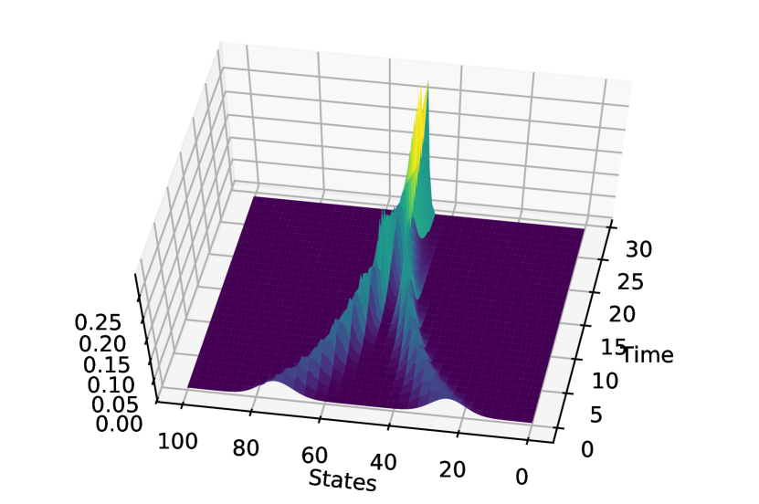
(a) Exact Solution

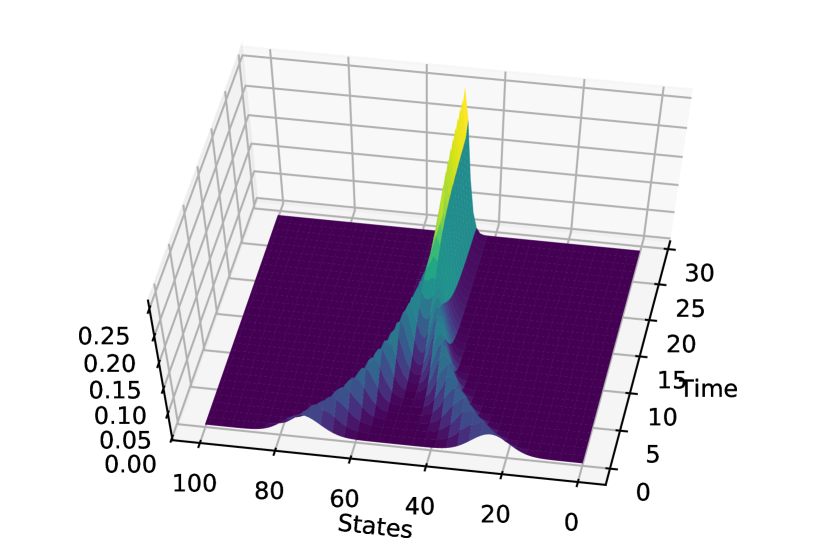
(b) Model-based

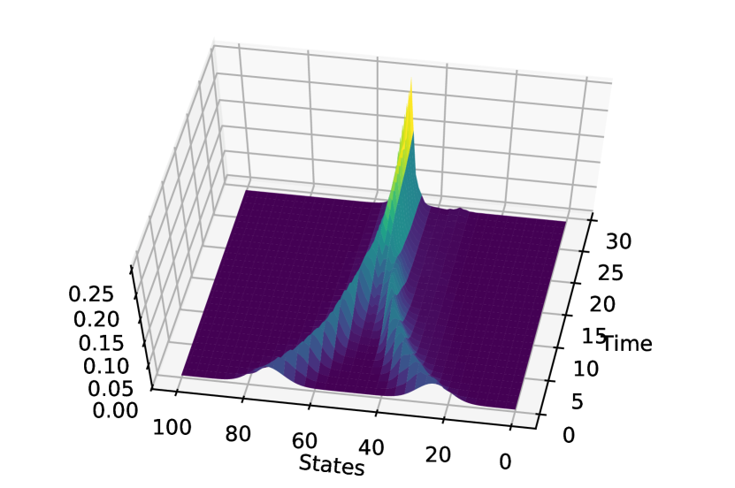
(c) Model-free

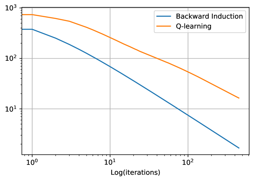
(d) Exploitability

Figure 1: Evolution of the distribution in the linear quadratic MFG with finite horizon.

Experimental setup: We consider a Linear Quadratic MFG with $100$ states and an horizon $N=30$, which provides a closed-form solution for the continuous state and action version of the game (see Appx. C) and bounds the number of actions $M=37$ required in the implementation. In practice, the variance $\sigma$ of the idiosyncratic noise $\epsilon_{n}$ is adapted to the number of states. Here, we set $\sigma=3$, $\Delta_{n}=0.1$, $K=1$, $q=0.01$, $\kappa=0.5$ and $c_{\rm term}=1$. In all the experiments, we set the learning rate $\alpha$ of $Q$-learning to 0.1 and the $\varepsilon$-greedy exploration parameter to $0.2$.

Numerical results: Figure 1 illustrates the convergence of Fictitious Play model-based and model-free algorithm in such context. The initial distribution, which is set to two separated bell-shaped distributions, are both driven towards $m$ and converge to a unique bell-shaped distribution as expected. The parameter $\sigma$ of the idiosyncratic noise influences the variance of the final normal distribution. We can observe that both Backward Induction and $Q$-learning provide policies that approximate this behaviour, and that the exploitability decreases with a rate close to $O(1/t)$ in the case of the model-based approach, while the model-free decreases more slowly.

4.2 The Beach Bar Process

Figure 2: The beach bar process.

As a second illustration, we now consider the beach bar process, a more involved monotone second order MFG with discrete state and action spaces, that does not offer a closed-form solution but can be analyzed intuitively. This example is a simplified version of the well known Santa Fe bar problem, which has received a strong interest in the MARL community, see e.g. [14, 55].

Environment: The beach bar process (Figure 2) is a Markov Decision Process with $|\mathcal{X}|$ states disposed on a one dimensional torus ($\mathcal{X}=\{0,\dots,|\mathcal{X}|-1\}$), which represents a beach. A bar is located in one of the states. As the weather is very hot, players want to be as close as possible to the bar, while keeping away from too crowded areas. Their dynamics is governed by the following equation:

$$x_{n+1}=x_{n}+b(x_{n},a_{n})+\epsilon_{n}$$

where $b$ is the drift, allowing the representative player to either stay still or move one node to the left or to the right. The additional noise $\epsilon_{n}$ can push the player one node away to the left or to the right with a small probability:

$$b(x_{n},a_{n})=\left\{\begin{array}[]{ll}1&\mbox{ if }a_{n}=\mbox{right}\\ 0&\mbox{ if }a_{n}=\mbox{still}\\ -1&\mbox{ if }a_{n}=\mbox{left}\end{array}\right. \epsilon_{n}=\left\{\begin{array}[]{ll}1&\mbox{ with probability }\frac{1-p}{2}\\ 0&\mbox{ with probability }p\\ -1&\mbox{ with probability }\frac{1-p}{2}\end{array}\right.$$ (15)

Therefore, the player can go up to two nodes right or left and it receives, at each time step, the reward:

$$r(x_{n},a_{n},\mu_{n})=\tilde{r}(x_{n})-\frac{|a_{n}|}{\mathcal{|X|}}-\log(\mu_{n}(x_{n}))\;,$$

where $\tilde{r}(x_{n})$ denotes the distance to the bar, whereas the last term represents the aversion of the player for crowded areas in the spirit of [11].

Numerical results: We conduct an experiment with 100 states and an horizon $N=15$. Starting from a uniform distribution, we can observe in Figure 3 that both backward induction and $Q$-learning algorithms converge quickly to a peaky distribution where the representative player intends to be as close as possible to the bar while moving away if the bar is already too crowded. The exploitability offers a nice way to measure how close we are from the Nash equilibrium and shows as expected that the model-based algorithm (backward induction) converges at a rate $O(1/t)$ and faster than the model-free algorithm ($Q$-learning).

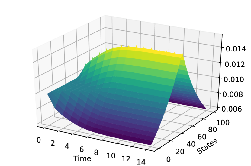
(a) Model-based

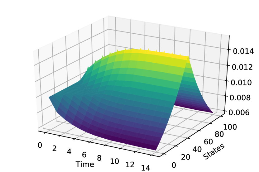
(b) Model-free

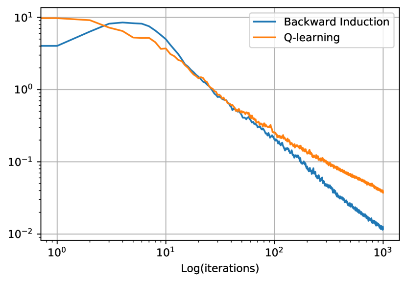
(c) Exploitability

Figure 3: Beach bar process in finite horizon: (a, b) evolution of the distribution, (c) exploitability.

5 Finite Horizon Mean Field Games with Common Noise

We now turn to the consideration of so-called MFG with common noise, that is including an additional discrete and common source of randomness in the dynamics. Players still sequentially take actions ($a\in\mathcal{A}$) in a state space $\mathcal{X}$, but the dynamics and the reward are affected by a common noise sequence $\{\xi_{n}\}_{0\leq n\leq N}$. We denote $\Xi_{n}=\{\xi_{k}\}_{0\leq k<n}=\Xi_{n-1}.\xi_{n-1}$ where $|\Xi_{n}|$ represents the total length of the sequence. The extra common source of randomness $\xi$ affects both the reward $r(x,a,\mu,\xi)$ and the probability transition function $p(x^{\prime}|x,a,\xi)$. We consider policies $\pi_{n}(a|x,\Xi)$ and population distribution $\mu_{n}(x|\Xi)$ which are both noise-dependent, and will simply be denoted $\pi_{n,\Xi}(a|x)$ and $\mu_{n|\Xi}(x)$. The $Q$ function is defined as:

$$Q^{\pi,\mu}_{N}(x,a|\Xi_{N})=r(x,a,\mu_{N|\Xi_{N}},\xi_{N}),\quad Q^{\pi,\mu}_{n-1}(x,a|\Xi_{n-1})=\sum\limits_{\xi}P(\xi_{n-1}=\xi|\Xi_{n-1})\Big{[}$$ (16)

$$\qquad r(x,a,\mu_{n-1,\Xi_{n-1}},\xi)+\sum\limits_{x^{\prime}\in\mathcal{X}}p(x^{\prime}|x,a,\xi)\mathbb{E}_{b\sim\pi_{n}(.|x^{\prime},\Xi_{n-1}.\xi)}\left[Q^{\pi,\mu}_{n}(x^{\prime},b|\Xi_{n-1}.\xi)\right]\Big{]},$$ (17)

while the value function is simply $V_{n}^{\pi,\mu}(x,\Xi_{n})=\mathbb{E}_{a\sim\pi_{n,\Xi_{n}}(.|x)}\left[Q^{\pi,\mu}_{n}(x,a|\Xi_{n})\right]$. Similarly, the distribution over states is conditioned on the sequence of noises and satisfies the balance equation: $\mu^{\pi}_{0}(x,\Xi_{0})=\mu_{0}(x)$ (with $\Xi_{0}$ being the empty sequence $\{\}$) and $\mu^{\pi}_{n+1}(x^{\prime}|\Xi.\xi)=\sum\limits_{x\in\mathcal{X}}p^{\pi_{n,\Xi.\xi}}(x^{\prime}|x,\xi)\mu^{\pi}_{n}(x|\Xi)$. The expected return for a representative player starting at $\mu_{0}$ is:

$$J(\mu_{0},\pi,\mu)=\sum_{x\in\mathcal{X}}\mu_{0}(x)V^{\pi,\mu}_{0}(x,\Xi_{0})=\sum_{n=0}^{N}\,\,\sum_{\Xi,\xi,|\Xi|=n}P(\Xi.\xi)\sum_{x\in\mathcal{X}}\left[\mu_{n}(x,\Xi)r(x,a,\mu_{n,\Xi},\xi)\right]$$ (18)

with $P(\Xi_{0})=1$ and $P(\Xi.\xi)=P(\xi|\Xi)P(\Xi)$. Finally the exploitability is again defined as:

$$\phi(\pi)=\max_{\pi^{\prime}}J(\mu_{0},\pi^{\prime},\mu^{\pi})-J(\mu_{0},\pi,\mu^{\pi}).$$ (19)

Continuous time Fictitious Play for MFGs with common noise: The Fictitious play process on MFGs with common noise is as follows. For $t<1$, we start with an arbitrary policy $\bar{\pi}^{t<1}$ (by convention we will take $\bar{\pi}^{t}=\pi^{\text{BR},t}$ for $t<1$) whose distribution is $\bar{\mu}^{t<1}=\mu^{\pi^{t<1}}$ (with the convention that $\bar{\mu}^{t}=\mu^{\text{BR},t}$). Then, for all $t$ and $\Xi$:

$$\bar{\mu}_{n}^{t}(x|\Xi)=\frac{1}{t}\int\limits_{s=0}^{t}\mu_{n}^{\text{BR},s}(x|\Xi)ds,$$ (20)

where $\mu^{\text{BR},t}$ is the distribution of a best response policy $\pi^{\text{BR},t}$ against $\bar{\mu}^{t}$ when $t\geq 1$. The distribution $\mu^{t}$ is the distribution of a policy $\bar{\pi}^{t}$, which is defined as follows for $t\geq 1$:

$$\forall n,\Xi,\qquad\;\bar{\pi}_{n}^{t}(a|x,\Xi)\int\limits_{s=0}^{t}\mu^{\text{BR},s}_{n}(x|\Xi)ds=\int\limits_{s=0}^{t}\mu^{\text{BR},s}_{n}(x|\Xi)\pi^{\text{BR},s}_{n}(a|x,\Xi)ds.$$ (21)

Theorem 2.

Under the monotony assumption, the exploitability is a strong Lyapunov function of the system for $t\geq 1$: $\frac{d}{dt}\phi(\bar{\pi}^{t})\leq-\frac{1}{t}\phi(\bar{\pi}^{t}).$ Therefore, $\phi(\bar{\pi}^{t})=O(\frac{1}{t})$.

6 Experiments with Common Noise

6.1 Linear Quadratic Mean Field Game

Environment: We use a similar environment as the one described in the Linear Quadratic MFG. On top of the idiosyncratic noise $\epsilon_{n}$, we add a common noise $\xi_{n}$, which is assumed to be stationary and i.i.d. We now consider the following dynamics:

$$x_{n+1}=x_{n}+(K(m_{n}-x_{n})+a_{n})\Delta_{n}+\sigma(\rho\xi_{n}+\sqrt{1-\rho^{2}}\epsilon_{n})\sqrt{\Delta_{n}}\;.$$ (22)

The reward remains unchanged, except that the first moment of the state distribution $\bar{\mu}_{n}$ now depends on the sequence of common noises $\Xi_{n}$: $m_{n}=\mathbb{E}[x_{n}|\Xi_{n}]$. We set $\rho=0.5$.

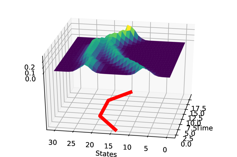
(a) Exact Solution

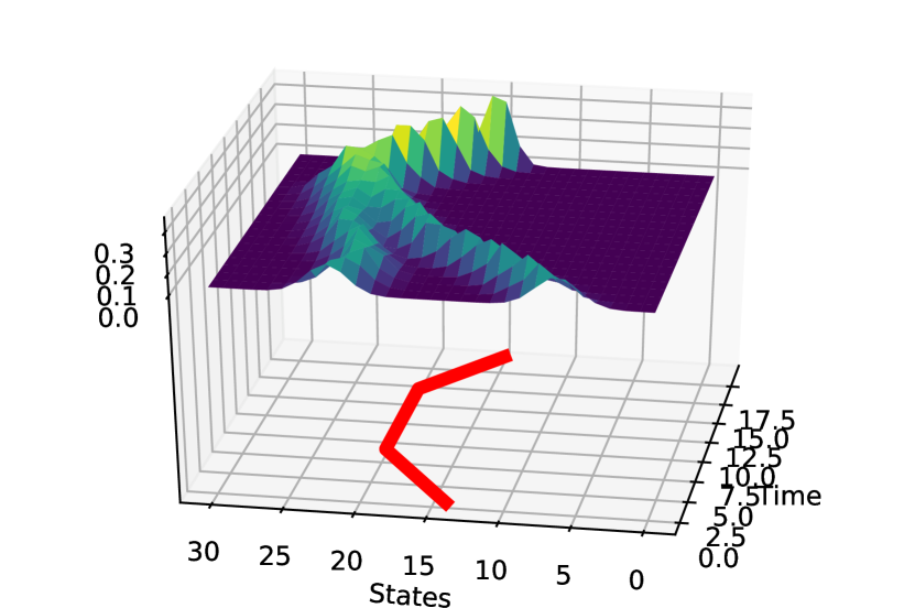
(b) Model-based

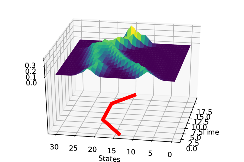
(c) Model-free

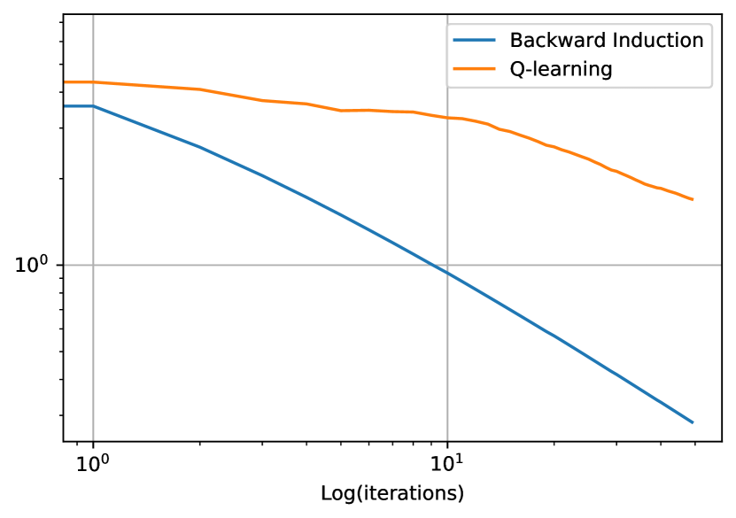
(d) Exploitability

Figure 4: Linear Quadratic with Common Noise.

Numerical results: On Figure 4, the two separated bell-shaped distributions reassemble and follow the sequence of common noises. Namely, the mean of the distribution moves with the successive common noises, which are represented by the red line below the distribution’s evolution. This evolution can be interpreted as a school of fish which undergoes a water flow (i.e. the sequence of common noises). Both model-based and model-free approaches approximate the exact solution. The exploitability of model-based still decreases at a rate $O(1/t)$, while the one of model-free decreases more slowly.

6.2 The Beach Bar Process

Environment: We consider a setting where the bar can close at only one given time step. This gives two possible realizations of the common noise: (1) the bar stays open or (2) it closes at this time step. Here, the dynamics remain unchanged but the reward now depends on the common noise: $r_{open}$ is the same reward as before, whereas $r_{closed}(x_{n},a_{n},\mu_{n})=-\frac{|a_{n}|}{\mathcal{|X|}}-\log(\mu_{n}(x_{n}))$.

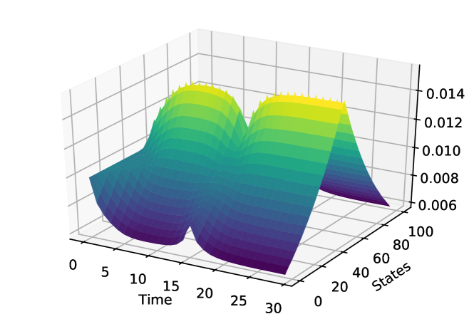
(a) Model-based, the bar stays open

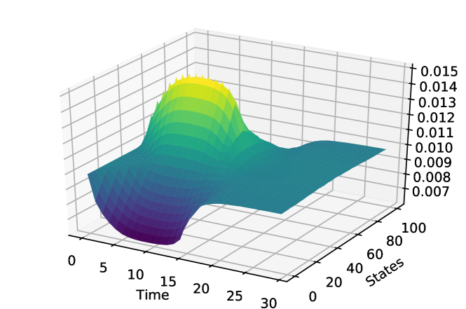
(b) Model-based, the bar closes

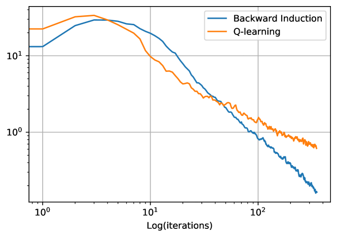
(c) Exploitability

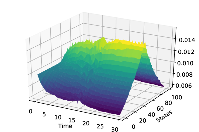
(d) Model-free, the bar stays open

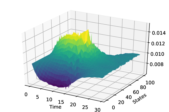
(e) Model-free, the bar closes

Figure 5: First Common Noise setting, the bar has a probability $0.5$ of closing at time step $15$.

Numerical results: We set the time step of closure at $\frac{N}{2}$ where $N=30$ is the horizon of the game and the number of states $\mathcal{|X|}$ to $100$. We choose the probability of closure to be $0.5$. Figure 5 shows that the players anticipate the possibility that the bar may close: the density of people next to the bar decreases before the time step of the common noise. After the common noise, the distribution becomes uniform if the bar has closed or people go back next to the bar if the bar stays open. Once again, the exploitability indicates that the model-based and model-free approaches both converge to the Nash equilibrium and that the model-based converges faster.

7 Experiment at Scale

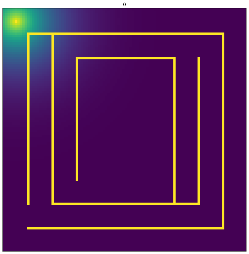
(a) Start

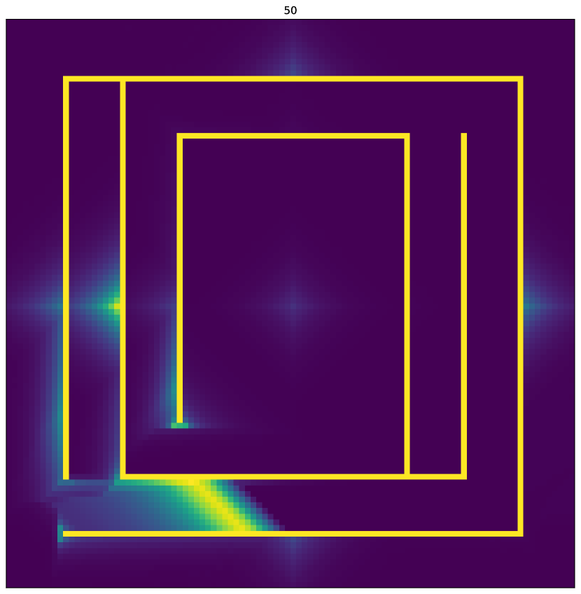
(b) Middle

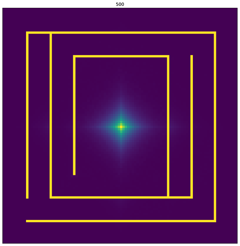
(c) End

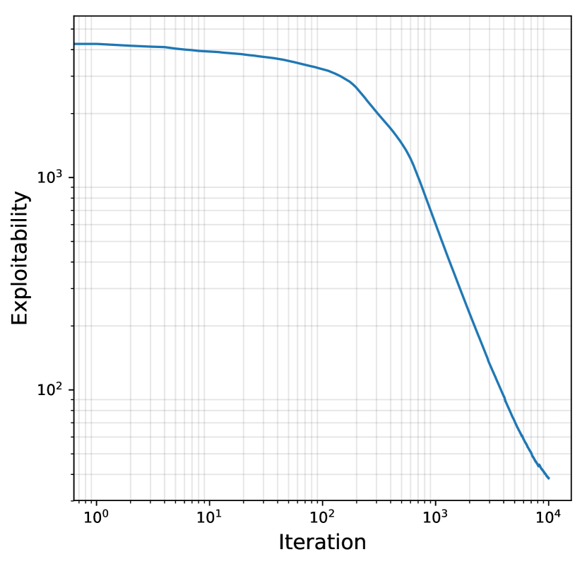
(d) Exploitability

Figure 6: 2D crowd modeling example.

We finally present a crowd modeling experiment, motivated by swarm robotics (see e.g. [88, 113, 48]), where a distribution of players is encouraged to move in a maze towards the center of a $100\times 100$ grid. The reward at a state $(i,j)$ is described as $r(s=(i,j),a,\mu)=10*(1-\frac{\|(i,j)-(50,50)\|_{1}}{100})-\frac{1}{2}\log(\mu(x))$, where the last term captures the aversion for crowded areas. The initial distribution is chosen proportional to $(1-\frac{\|(i,j)-(5,5)\|_{2}}{\sqrt{2\times 95^{2}}})^{10}$ while being null on the maze obstacles (the yellow strait lines). The evolution of the distribution as well as the exploitability are represented in Figure 6 (a video is available in supplementary material).

8 Related Work

Theoretical results in MFGs: Theoretical results in terms of uniqueness, existence and stability of Nash equilibrium in such games are numerous, see [30, 19, 36]. A key motivation is that the optimal control derived in an MFG provides an approximate Nash equilibrium in a game with a large but finite number of players. In general, most games are considered in a continuous setting while Gomes et al. [62] proved existence results for finite state and action spaces MFGs and [99] considered finite state discounted cost MFGs. An important and challenging extension is the case of players sharing a common source of risk (such as several companies in the same economy market), giving rise to the so-called MFG with common noise, see [37] or [36, Volume II]. These games are usually solved by numerical methods for partial differential equations [9] or probabilistic methods [12, 40, 59].

Learning in games and MFGs: The scaling limitations of traditional multi-agent learning methods with respect to the number of players remain quite hard to overcome as the complexity of independent learning methods [56, 96, 95, 109, 92, 58, 57] scales at least linearly with the number of players and some methods may scale exponentially (e.g. Nash $Q$-learning [74] or correlated $Q$-learning [66]). By approximating the discrete population by a continuous one, the MFG scheme made learning approaches more suitable and attracted a surge of interest. Model-based methods have been first considered (e.g.  [116] studied a MF oscillator game, [31] initiated the study of Fictitious Play in MFGs). Recently, several works have focused on model-free methods such as $Q$-learning [68] but the convergence results rely on very strong hypotheses. Note that, although our method can make use of $Q$-learning to learn a best response, it does not rely on it. Also, our method can make use of both model-based and model-free algorithms. Finally, our method relies only on the Lasry-Lions monotonicity condition, which is much less restrictive than a potential or variational structure.

Fictitious Play (FP), which is also a classical method to learn in $N$-player games [97, 93, 71, 73, 72, 96], combined with a model-free algorithm has been considered in [90] but with several inaccuracies, as already pointed out in [111], which focuses on policy gradient methods. However, they study a restricted stationary setting as opposed to the finite time horizon covered by our contribution and their convergence results hold under hardly verifiable assumptions.

Convergence of approximate FP has been proved in [54] (based on the FP analysis of [69]) but without common noise and their analysis is for discrete time FP and only for first-order MFGs (without noise in the dynamics). Our analysis, done in continuous time, is more transparent and works for MFGs with both idiosyncratic and common sources of randomness in the dynamics. Furthermore, their numerical example was stationary whereas we were also able to learn the solution of time-dependent MFGs, which covers a larger scope of meaningful applications. Finally, our analysis provides a rate of convergence ($O(\frac{1}{t})$) while previous FP work in MFG do not.

9 Conclusion

In this paper we have shown that Fictitious Play can serve as a basis for building practical algorithms to solve a wide variety of MFGs including finite horizon and $\gamma$-discounted MFGs as well as games perturbed by a common noise. We proved that, in all these settings, the resulting exploitability decreases at a rate of $O(\frac{1}{t})$ and that this metrics can be used to monitor the quality of the control throughout the learning. To illustrate our findings and the versatility of the method, we instantiated the Fictitious Play scheme using Backward Induction and $Q$-Learning to learn intermediate best responses. Application of these instances on different MFGs have shown that the proposed algorithms consistently learned a near-optimal control and led to the desired behaviour for the population of players. This scheme has the potential to scale up dramatically by using advanced reinforcement learning algorithms combined with neural networks for the computation of the best response.

Broader Impact

Applications of MFGs: The MFG model has inspired numerous applications [67] and we hope our work can help practitioners to solve MFGs problems at scale. A popular application focuses on population dynamics modeling [1, 33] including crowd motion modeling [7, 27, 46, 16, 8, 43], opinion dynamics and consensus formation [110, 18, 94], autonomous vehicles [75, 105] or sanitary vaccination [77, 51]. But MFGs have also naturally found applications in banking, finance and economics including banking systemic risk [38, 52], high frequency trading [82, 32], income and wealth distribution [6], economic contract design [53], economics in general [6, 2, 41, 61, 47] or price formation [84, 82, 63]. Energy management or production applications are studied in [10, 44, 50, 17, 79, 85, 67, 5, 42, 65], whereas security and communication applications appear in [89, 100, 70, 115, 80, 81].

Exploitability as a metric: One of the leading factor of progress for numerical or learning methods is the clear understanding of which metrics should be optimized. In reinforcement learning, the mean human normalized score is a standard metric of success. In supervised learning, the top 1 accuracy has been the foremost metric of success. We hope the exploitability can achieve such a role on the numerical aspects of MFGs.

Appendix A Continuous Time Fictitious Play in Finite Horizon

In this section, we prove the Fictitious Play convergence result in the absence of common noise. For the sake of clarity, we will write:

$$r^{\pi}(x,\mu)=\mathbb{E}_{a\sim\pi(.|x)}\left[r(x,a,\mu)\right]\quad\mbox{ and }\quad p^{\pi}(x^{\prime}|x)=\mathbb{E}_{a\sim\pi(.|x)}\left[p(x^{\prime}|x,a)\right]$$

for the rest of this section.

First, we prove the following property, which stems from monotonicity.

Property 1.

Let $f$ be a smooth enough function and let assume that the ODE $\dot{\mu}=f(\mu)$ (with $\dot{\mu}=\frac{d}{dt}\mu$) has a solution $(\mu^{t})_{t\geq 0}=(\mu^{t}_{n}(x))_{t\geq 0,x\in\mathcal{X}}$. If the game is monotone, then:

$$\sum\limits_{x\in\mathcal{X}}<\nabla_{\mu}\bar{r}(x,\mu),\dot{\mu}>\dot{\mu}(x)\leq 0.$$

Proof.

The monotonicity condition implies that, for all $\tau\geq 0$, we have:

$$\sum\limits_{x\in\mathcal{X}}(\mu^{t}(x)-\mu^{t+\tau}(x))(\bar{r}(x,\mu^{t})-\bar{r}(x,\mu^{t+\tau}))\leq 0.$$

Thus:

$$\sum\limits_{x\in\mathcal{X}}\frac{\mu^{t}(x)-\mu^{t+\tau}(x)}{\tau}\frac{\bar{r}(x,\mu^{t})-\bar{r}(x,\mu^{t+\tau})}{\tau}\leq 0.$$

The result follows when $\tau\rightarrow 0$. ∎

Property 2.

Let $\hat{\pi}^{t}=(\hat{\pi}^{t}_{n})_{n=0,\dots,N}$ be a sequence of time-dependent policies and let $\mu^{\hat{\pi}^{t}}=(\mu^{\hat{\pi}^{t}}_{n}(x))_{n=0,\dots,N,x\in\mathcal{X}}$ be the sequence of their distributions over states. Let us denote, for all $t,n,x$, $\bar{\mu}_{n}^{t}(x)=\frac{1}{t}\int\limits_{0}^{t}\mu_{n}^{\hat{\pi}^{s}}(x)ds$. Then, the policy generating this average distribution is:

$$\bar{\pi}_{n}^{t}(a|x)=\frac{\int\limits_{0}^{t}\mu_{n}^{\hat{\pi}^{s}}(x)\hat{\pi}_{n}^{s}(a|x)ds}{\int\limits_{0}^{t}\mu_{n}^{\hat{\pi}^{s}}(x)ds}.$$ (23)

Note that $\int\limits_{0}^{t}\mu_{n}^{\hat{\pi}^{s}}(x)ds$ can be chosen to be strictly positive as one can choose an arbitrary policy on the time interval $[0,1]$ (for example, the uniform policy).

Or, more simply, one can write:

$$\bar{\mu}_{n}^{t}(x)\bar{\pi}_{n}^{t}(a|x)=\frac{1}{t}\int\limits_{0}^{t}\mu_{n}^{\hat{\pi}^{s}}(x)\hat{\pi}_{n}^{s}(a|x)ds.$$ (24)

Moreover, we have:

$$\dot{\bar{\mu}}_{n}^{t}(x)\bar{\pi}_{n}^{t}(a|x)+\bar{\mu}_{n}^{t}(x)\dot{\bar{\pi}}_{n}^{t}(a|x)=\frac{1}{t}\left[\mu_{n}^{\hat{\pi}^{t}}(x)\hat{\pi}^{t}(a|x)-\bar{\mu}_{n}^{\hat{\pi}^{t}}(x)\bar{\pi}_{n}^{t}(a|x)\right].$$ (25)

Proof.

Let us start with the following equality, which holds by definition of the dynamics:

$$\mu_{n+1}^{\hat{\pi}^{s}}(x^{\prime})=\sum\limits_{x\in\mathcal{X}}\sum\limits_{a\in\mathcal{A}}p(x^{\prime}|x,a)\hat{\pi}_{n}^{s}(a|x)\mu_{n}^{\hat{\pi}^{s}}(x).$$ (26)

Then, taking on both sides the average over the Fictitious Play time yields:

$$\frac{1}{t}\int\limits_{0}^{t}\mu_{n+1}^{\hat{\pi}^{s}}(x^{\prime})ds=\sum\limits_{x\in\mathcal{X}}\sum\limits_{a\in\mathcal{A}}p(x^{\prime}|x,a)\frac{1}{t}\int\limits_{0}^{t}\hat{\pi}_{n}^{s}(a|x)\mu_{n}^{\hat{\pi}^{s}}(x)ds.$$ (27)

The left hand side is $\bar{\mu}_{n+1}^{t}(x^{\prime})$ by definition, and the time average in the right hand side can be written as:

$$\frac{1}{t}\int\limits_{0}^{t}\hat{\pi}_{n}^{s}(a|x)\mu_{n}^{\hat{\pi}^{s}}(x)ds=\frac{\int\limits_{0}^{t}\hat{\pi}_{n}^{s}(a|x)\mu_{n}^{\hat{\pi}^{s}}(x)ds}{\int\limits_{0}^{t}\mu_{n}^{\hat{\pi}^{s}}(x)ds}\frac{1}{t}\int\limits_{0}^{t}\mu_{n}^{\hat{\pi}^{s}}(x)ds=\bar{\mu}_{n}^{\hat{\pi}^{t}}(x)\bar{\pi}_{n}^{t}(a|x).$$

Combining the terms, we obtain:

$$\bar{\mu}_{n+1}^{t}(x^{\prime})=\sum\limits_{x\in\mathcal{X}}\sum\limits_{a\in\mathcal{A}}p(x^{\prime}|x,a)\bar{\mu}_{n}^{\hat{\pi}^{t}}(x)\bar{\pi}_{n}^{t}(a|x),$$

which proves that the policy $\bar{\pi}_{n}^{t}$ defined in (23) indeed generates $\bar{\mu}_{n}^{t}$. The other equalities in the statement can be deduced from here readily. ∎

Based on the above properties, we now proceed to the proof of the convergence of Fictitious Play (Theorem 1) in the finite horizon case.

Proof of Theorem 1.

To alleviate the notation, given a policy $\pi$, we denote:

$$r^{\pi}(x,\mu)=\sum_{a}\pi(a|x)r(x,a,\mu).$$

We start by noticing that, thanks to the structure of the reward coming from the monotonicity assumption,

$$\nabla_{\mu}r^{\pi_{n}^{\text{BR},t}}(x,\bar{\mu}_{n}^{t})=\nabla_{\mu}\bar{r}(x,\bar{\mu}_{n}^{t})\textrm{ and }\nabla_{\mu}r^{\pi_{n}}(x,\bar{\mu}_{n}^{t})=\nabla_{\mu}\bar{r}(x,\bar{\mu}_{n}^{t}).$$ (28)

Moreover, from Property 2 with $\pi$ replaced by $\hat{\pi}^{\text{BR}}$ and $\mu^{\hat{\pi}^{t}}$ replaced by $\mu^{\text{BR},t}$, we obtain (24). Dropping the overlines to alleviate the presentation (so $\mu^{t}$ and $\pi^{t}$ denote respectively the average sequence of distributions and the average sequence of policies), it implies:

$$\mu_{n}^{t}(x)\frac{d}{dt}\pi_{n}^{t}(a|x)=\frac{1}{t}\mu^{\text{BR},t}_{n}(x)[\pi^{\text{BR},t}_{n}(a|x)-\pi_{n}^{t}(a|x)].$$ (29)

Moreover, recall that:

$$\frac{d}{dt}\mu_{n}^{t}(x)=\frac{1}{t}\left[\mu^{\text{BR},t}_{n}(x)-\mu_{n}^{t}(x)\right].$$ (30)

From the above observations, we deduce successively:

$$\frac{d}{dt}\phi(\pi^{t}) =\frac{d}{dt}\left[\max\limits_{\pi^{\prime}}J(\mu_{0},\pi^{\prime},\mu^{t})-J(\mu_{0},\pi^{t},\mu^{t})\right]$$

$$=\sum\limits_{n=0}^{N}\sum\limits_{x\in\mathcal{X}}\Big{[}<\nabla_{\mu}r^{\pi_{n}^{\text{BR}}}(x,\mu_{n}^{t}),\frac{d}{dt}\mu_{n}^{t}>\mu^{\text{BR},t}_{n}(x)-<\nabla_{\mu}r^{\pi_{n}}(x,\mu_{n}^{t}),\frac{d}{dt}\mu_{n}^{t}>\mu_{n}^{t}(x)$$

$$\qquad\qquad\qquad\qquad-<\frac{d}{dt}\pi_{n}^{t}(.|x),r(x,.,\mu_{n}^{t})>\mu_{n}^{t}(x)-r^{\pi_{n}}(x,\mu_{n}^{t})\frac{d}{dt}\mu_{n}^{t}(x)\Big{]}$$

$$=\sum\limits_{n=0}^{N}\sum\limits_{x\in\mathcal{X}}\left[t<\nabla_{\mu}\bar{r}(x,\mu_{n}^{t}),\frac{d}{dt}\mu_{n}^{t}>\frac{1}{t}\left(\mu^{\text{BR},t}_{n}(x)-\mu_{n}^{t}(x)\right)\right]$$

$$\qquad+\sum\limits_{n=0}^{N}\sum\limits_{x\in\mathcal{X}}\left[\frac{1}{t}r^{\pi_{n}}(x,\mu_{n}^{t})\mu_{n}^{t}(x)-\frac{1}{t}r^{\pi_{n}^{\text{BR},t}}(x,\mu_{n}^{t})\mu_{n}^{\text{BR},t}(x)\right]$$

$$=-\frac{1}{t}\phi(\pi^{t})+\sum\limits_{n=0}^{N}\sum\limits_{x\in\mathcal{X}}\left[t<\nabla_{\mu}\bar{r}(x,\mu_{n}^{t}),\frac{d}{dt}\mu_{n}^{t}>\frac{d}{dt}\mu_{n}^{t}(x)\right],$$

where the third equality holds by (28),  (29) and (30). Note that the product $<\nabla_{\mu}\bar{r}(x,\mu_{n}^{t}),\frac{d}{dt}\mu_{n}^{t}>$ in the last sum above is non-positive thanks to Property 1 (i.e., thanks to the monotonicity assumption). Hence, the conclusion holds. ∎

Appendix B Continuous Time Fictitious Play in Finite Horizon with Common Noise

In this section, we prove the convergence result of continuous time Fictitious Play in finite horizon MFGs with common noise (Theorem 2). The reasoning is similar as in the finite horizon case without common noise (Appx. A). The only difference comes from the conditioning with the common noise.

Proof of Theorem 2.

For any policy, recall that we write $\pi_{n,\Xi}^{t}(a|x)=\pi_{n}^{t}(a|x,\Xi)$.

We first note that, by the structure of the reward function, we have,

$$\nabla_{\mu}r^{\pi_{n,\Xi.\xi}^{\text{BR},t}}(x,\mu_{n|\Xi}^{t})=\nabla_{\mu}\bar{r}(x,\mu_{n|\Xi}^{t})\textrm{ and }\nabla_{\mu}r^{\pi_{n,\Xi.\xi}}(x,\mu_{n|\Xi}^{t})=\nabla_{\mu}\bar{r}(x,\mu_{n|\Xi}^{t}).$$

Moreover,

$$-<\frac{d}{dt}\pi_{n,\Xi.\xi}^{t}(.|x),r(x,.,\mu_{n|\Xi}^{t})>\mu_{n|\Xi}^{t}(x)=-\frac{1}{t}r^{\pi_{n,\Xi.\xi}^{\text{BR},t}}(x,\mu_{n|\Xi}^{t})\mu_{n|\Xi}^{\text{BR},t}(x)+\frac{1}{t}r^{\pi_{n,\Xi.\xi}}(x,\mu_{n|\Xi}^{t})\mu_{n|\Xi}^{\text{BR},t}(x)$$

and

$$-r^{\pi_{n,\Xi.\xi}}(x,\mu_{n|\Xi}^{t})\frac{d}{dt}\mu_{n|\Xi}^{t}(x)=\frac{1}{t}r^{\pi_{n,\Xi.\xi}}(x,\mu_{n|\Xi}^{t})\mu_{n|\Xi}^{t}(x)-\frac{1}{t}r^{\pi_{n,\Xi.\xi}}(x,\mu_{n|\Xi}^{t})\mu^{\text{BR},t}_{n}(x)$$

Using the definition of exploitability together with the above remarks, we deduce:

$$\frac{d}{dt}\phi(\pi^{t})=\frac{d}{dt}\left[\max\limits_{\pi^{\prime}}J(\mu_{0},\pi^{\prime},\mu^{\pi})-J(\mu_{0},\pi,\mu^{\pi})\right]$$ (31)

$$=\sum\limits_{n=0}^{N}\,\,\sum_{\Xi,|\Xi|=n}\sum_{\xi}P(\Xi.\xi)\sum\limits_{x\in\mathcal{X}}\Big{[}<\nabla_{\mu}r^{\pi_{n,\Xi.\xi}^{\text{BR}},\xi}(x,\mu_{n|\Xi}^{t}),\frac{d}{dt}\mu_{n|\Xi}^{t}>\mu^{\text{BR},t}_{n,\Xi.\xi}(x)$$ (32)

$$\qquad\qquad-<\nabla_{\mu}r^{\pi_{n,\Xi.\xi}}(x,\mu_{n|\Xi}^{t},\xi),\frac{d}{dt}\mu_{n|\Xi}^{t}>\mu_{n|\Xi}^{t}(x)$$ (33)

$$\qquad\qquad-<\frac{d}{dt}\pi_{n,\Xi.\xi}^{t}(.|x),r(x,.,\mu_{n|\Xi}^{t})>\mu_{n|\Xi}^{t}(x)-r^{\pi_{n,\Xi.\xi}}(x,\mu_{n|\Xi}^{t})\frac{d}{dt}\mu_{n|\Xi}^{t}(x)\Big{]}$$ (34)

$$=\sum\limits_{n=0}^{N}\,\,\sum_{\Xi,|\Xi|=n}\sum_{\xi}P(\Xi.\xi)\sum\limits_{x\in\mathcal{X}}\Big{[}t<\nabla_{\mu}\bar{r}(x,\mu_{n|\Xi}^{t})),\frac{d}{dt}\mu_{n|\Xi}^{t}>\frac{1}{t}\left(\mu^{\text{BR},t}_{n|\Xi}(x)-\mu_{n|\Xi}^{t}(x)\right)\Big{]}$$ (35)

$$\qquad+\sum\limits_{n=0}^{N}\,\,\sum_{\Xi,|\Xi|=n}\sum_{\xi}P(\Xi.\xi)\sum\limits_{x\in\mathcal{X}}\big{[}\frac{1}{t}r^{\pi_{n,\Xi.\xi}}(x,\mu_{n|\Xi}^{t})\mu_{n|\Xi}^{t}(x)-\frac{1}{t}r^{\pi_{n,\Xi.\xi}^{\text{BR},t}}(x,\mu_{n|\Xi}^{t})\mu_{n|\Xi}^{\text{BR},t}(x)\big{]}$$ (36)

$$=-\frac{1}{t}\phi(\pi^{t})+\sum\limits_{n=0}^{N}\,\,\sum_{\Xi,|\Xi|=n}\sum_{\xi}P(\Xi.\xi)\sum\limits_{x\in\mathcal{X}}\big{[}t<\nabla_{\mu}\bar{r}(x,\mu_{n|\Xi}^{t}),\frac{d}{dt}\mu_{n|\Xi}^{t}>\frac{d}{dt}\mu_{n|\Xi}^{t}(x)\big{]},$$ (37)

where the last term is non-positive by Property 1 (i.e., thanks to the monotonicity assumption). ∎

Experiments: A More Complex Setting for the Beach Bar Process with common noise

Environment: Following the first setting of the paper where the bar could only close at one given time step, we now introduce a second more complex setting, bringing also of common noise in the beach bar process. Namely, the bar has a probability $p$ to close at every time step up to a point (in practice, this point is half of the horizon: $\frac{N}{2}$). Once the bar is closed, it does not open again. This setting gives $\frac{N}{2}+1$ possible realizations of the common noise: (1) the case where the bar never closes and (2) the $\frac{N}{2}$ cases where it closes at any of the first $\frac{N}{2}$ time steps. For the sake of clarity, we only present the evolution of the distributions when the bar finally remains open after $\frac{N}{2}$ time steps, and when it closes at the $\frac{N}{2}^{\text{th}}$ time step.

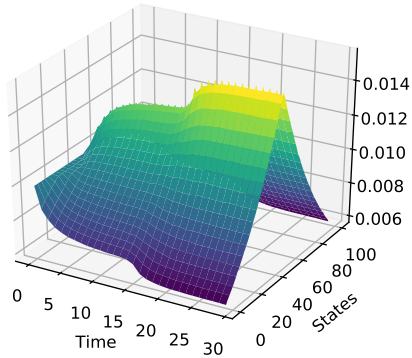
(a) Model-based, the bar stays open

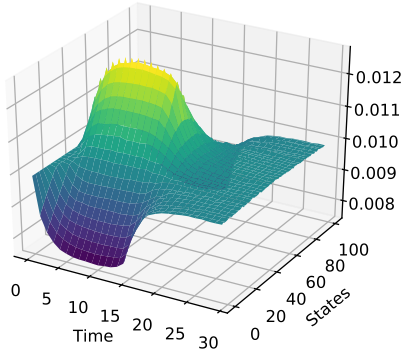
(b) Model-based, the bar closes

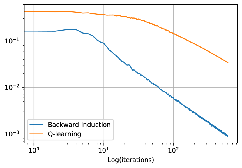
(c) Exploitability

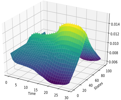
(d) Model-free, the bar stays open

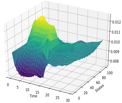
(e) Model-free, the bar closes

Figure 7: 2^nd common noise setting, the bar has a probability $p=0.5$ to close at every time step before $\frac{N}{2}$.

Numerical results: Similarly to the first setting, we take $|\mathcal{X}|=100$ states and $N=30$ time steps. As the bar has a probability $p=0.5$ to close at every time step until $\frac{N}{2}$, the distribution is flatter to anticipate the fact that people might need to spread. We can see that both model-based and model-free approaches converge to a Nash equilibrium and that model-based converges faster than model-free.

 

Appendix C Continuous Time Fictitious Play: the $\gamma$-discounted case

Surprisingly, the analysis also holds in the $\gamma$-discounted case with again the same style of reasoning. However, the distribution considered will be the $\gamma$-weighted occupancy measure instead of the distribution over states. In this section, we reintroduce the notations and we prove similar continuous time FP convergence results.

Consider, given the following:

• a finite state space $\mathcal{X}$ ($x\in\mathcal{X}$),

• a finite action space $\mathcal{A}$ ($a\in\mathcal{A}$),

• the set of distributions over state is $\Delta\mathcal{X}$ ($\mu\in\Delta\mathcal{X}$),

• a reward function $r(x,a,\mu)$,

• the transition function $p(x^{\prime}|x,a)$,

• a policy: $\pi(a|x)$.

We will write:

• $p^{\pi}(x^{\prime}|x)=\mathbb{E}_{a\sim\pi(.|x)}[p(x^{\prime}|x,a)]$,

• $r^{\pi}(x,\mu)=\mathbb{E}_{a\sim\pi(.|x)}[r(x,a,\mu)]$,

The cumulative $\gamma$-discounted reward is defined as:

$$J_{\gamma}(x_{0},\pi,\mu)=\mathbb{E}\left[\sum\limits_{n=0}^{+\infty}\gamma^{n}r(x_{n},a_{n},\mu)\;|\;x_{n+1}\sim p(.|x_{n},a_{n}),\;a_{n}\sim\pi(.|x_{n})\right]$$

Useful properties: We have $\mu_{\gamma}^{\pi}(x^{\prime})=\mu_{0}(x^{\prime})+\gamma\sum\limits_{x\in\mathcal{X}}p^{\pi}(x^{\prime}|x)\mu_{\gamma}^{\pi}(x)$ (in vectorial notations ${\mu_{\gamma}^{\pi}}^{\top}=\mu_{0}^{\top}(I-\gamma P^{\pi})^{-1}$).
The $\gamma$-discounted reward can be written as: $J_{\gamma}(x_{0},\pi,\mu)=\sum\limits_{x\in\mathcal{X}}\mu_{\gamma}^{\pi}(x)r^{\pi}(x,\mu)$.
We then have a similar formula for the policy generating the average distribution $\bar{\mu}^{\pi}_{\gamma}(x,t)=\frac{1}{t}\int\limits_{0}^{t}\mu_{\gamma}^{\pi}(x,s)ds$ can be written $\bar{\pi}_{\gamma}(a|x,t)=\frac{\int\limits_{0}^{t}\mu_{\gamma}^{\pi}(x,s)\pi(a|x,s)ds}{\int\limits_{0}^{t}\mu_{\gamma}^{\pi}(x,s)ds}$.

Finally, we can write:

$$\bar{\mu}_{\gamma}^{\pi}(x,t)\bar{\pi}_{\gamma}(a|x,t)=\frac{1}{t}\int\limits_{0}^{t}\mu_{\gamma}^{\pi}(x,s)\pi(a|x,s)ds$$ (38)

And:

$$\dot{\bar{\mu}}^{\pi}_{\gamma}(x,t)\bar{\pi}_{\gamma}(a|x,t)+\bar{\mu}^{\pi}_{\gamma}(x,t)\dot{\bar{\pi}}_{\gamma}(a|x,t)=\frac{1}{t}\left[\mu^{\pi}_{\gamma}(x,t)\pi(a|x,t)-\bar{\mu}^{\pi}_{\gamma}(x,t)\bar{\pi}_{\gamma}(a|x,t)\right].$$ (39)

Fictitious Play in MFGs: In the $\gamma$-discounted case, Fictitious Play can be written as (for $t\geq 1$):

$$\dot{\mu}(x,t)=\frac{1}{t}(\mu^{\text{BR}}_{\gamma}(x,t)-\mu(x,t))$$

where $\mu^{\text{BR}}_{\gamma}(x,t)$ is the distribution of a best response against $\mu(x,t)$ of policy $\pi^{\text{BR}}(a|x,t)$. In this section, we will write $\pi(a|x,t)$ the policy of the distribution $\mu(x,t)$. From Eq.(39), we can deduce the following property:

Property 3.

$$\forall n,\;\dot{\pi}(a|x,t)\mu(x,t)=\frac{1}{t}\mu^{\text{BR}}_{\gamma}(x,t)[\pi^{\text{BR}}(a|x,t)-\pi(a|x,t)]$$

Proof.

Such representation directly follows from Eq.(39). ∎

We are now in position to turn to the Lyapounov congerging property of the Fictitious process.

Property 4.

Under the monotony assumption, we can show that the exploitability ($\phi(t)=\max\limits_{\pi^{\prime}}J_{\gamma}(x_{0},\pi^{\prime},\mu^{\pi})-J_{\gamma}(x_{0},\pi,\mu^{\pi})$) is a strong Lyapunov function of the system:

$$\dot{\phi}(t)\leq-\frac{1}{t}\phi(t)$$

Proof.

$$\dot{\phi}(t)$$

$$=\sum\limits_{x\in\mathcal{X}}\big{[}\overbrace{<\nabla_{\mu}r^{\pi^{\text{BR}}}(x,\mu(t)),\dot{\mu}(t)>\mu^{\text{BR}}_{\gamma}(x,t)-<\nabla_{\mu}r^{\pi}(x,\mu(t)),\dot{\mu}(t)>\mu(x,t)}^{\textrm{With }\nabla_{\mu}r^{\pi^{\text{BR}}}(x,\mu(t))=\nabla_{\mu}\bar{r}(x,\mu(t))\textrm{ and }\nabla_{\mu}r^{\pi}(x,\mu(t))=\nabla_{\mu}\bar{r}(x,\mu(t))}$$

$$\underbrace{-<\dot{\pi}(.|x,t),r(x,.,\mu(t))>\mu(x,t)}_{=-\frac{1}{t}r^{\pi^{\text{BR}}}(x,\mu(t))\mu_{\gamma}^{\text{BR}}(x,t)+\frac{1}{t}r^{\pi}(x,\mu(t))\mu_{\gamma}^{\text{BR}}(x,t)}\underbrace{-r^{\pi}(x,\mu(t))\dot{\mu}(x,t)}_{=\frac{1}{t}r^{\pi}(x,\mu(t))\mu(x,t)-\frac{1}{t}r^{\pi}(x,\mu(t))\mu^{\text{BR}}_{\gamma}(x,t)}\big{]}$$

$$=\sum\limits_{x\in\mathcal{X}}\big{[}t<\nabla_{\mu}\bar{r}(x,\mu(t))),\dot{\mu}(t)>[\frac{1}{t}(\mu_{\gamma}^{\text{BR}}(x,t)-\mu(x,t))]\big{]}$$

$$\qquad+\sum\limits_{x\in\mathcal{X}}\big{[}\frac{1}{t}r^{\pi}(x,\mu(t))\mu(x,t)-\frac{1}{t}r^{\pi^{\text{BR}}}(x,\mu(t))\mu_{\gamma}^{\text{BR}}(x,t)\big{]}$$

$$=-\frac{1}{t}\phi(t)+\underbrace{\sum\limits_{x\in\mathcal{X}}\big{[}t<\nabla_{\mu}\bar{r}(x,\mu(t))),\dot{\mu}(t)>\dot{\mu}(x,t))\big{]}}_{\leq 0\textrm{ by monotony}}$$ (40)

$$\leq-\frac{1}{t}\phi(t)$$ (41)

∎

Experiment: the Beach Bar Process with $\gamma$-discounted reward.

Environment: We implement the beach bar process in the $\gamma$-discounted setting.

Numerical results: We set $\gamma=0.9$. The algorithm estimating the best response to a fixed distribution $\mu$ is Policy Iteration in the case of the model based approach and $Q$-learning in the model-free. As the flow of distributions converges towards the stationary distribution which is not time-dependant, we only plot the final distribution obtained after $300$ time steps (and not the evolution throughout time as before). In particular, we notice that model-based and model-free approaches converge towards the same distribution. We can also observe that the convergence rate of exploitability is $O(1/t)$ for the model-based and slower for the model-free approach.

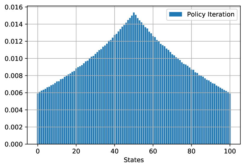
(a) Model-based

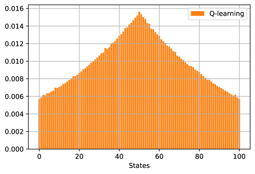
(b) Model-free

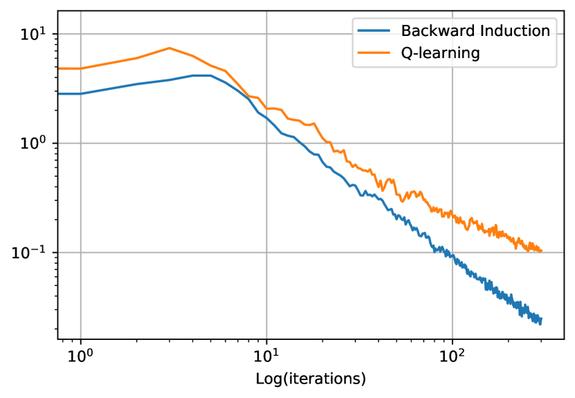
(c) Exploitability

Figure 8: Final distributions and exploitability in the $\gamma$-discounted case

Appendix D Algorithms

input : Start with a fixed distribution $\mu=(\mu_{k})_{k}$ and $Q^{k}=0$ and $\epsilon$ and the learning rate $\alpha$.

1 for $k=0,\dots,K$: do

2      sample $x^{k}_{0}\sim\mu_{0}$ ;

3      for $n=0,\dots,N$: do

4           $a_{n}^{k}$ is $\epsilon$-greedy with respect to $Q^{k}(x^{k}_{n},.)$.;

5           if not terminal sample $x_{n+1}^{k}$ according to $p(.|x^{k}_{n}a_{n}^{k})$.;

6           $Q^{k+1}_{n}(x^{k}_{n},a_{n}^{k})=(1-\alpha)Q^{k+1}_{n}(x^{k}_{n},a_{n}^{k})+\alpha[r(x^{k}_{n},a_{n}^{k},\mu_{k-1})+\max_{b}Q^{k}_{n+1}(x^{k}_{n+1},b)]$;

7          

8          

return $\pi^{*}$ a greedy policy with respect to $Q^{K}$

Algorithm 2 $Q$-Learning in Mean Field Games

input : Start with a fixed policy $\pi$ and an initial distribution $\mu_{0}=\mu^{\pi}_{0}$

1 for $k=0,\dots,K$: do

2      sample $x^{k}_{0}\sim\mu_{0}$ ;

3      for $n=0,\dots,N$: do

4           $a_{n}^{k}$ with respect to $Q^{k}(x^{k}_{n},.)$.;

5           if not terminal sample $x_{n+1}^{k}$ according to $p(.|x^{k}_{n}a_{n}^{k})$.

6          

7           Finally $\forall x,n\in\mathcal{X}\times\{0,\dots,N\}\;\hat{\mu}^{\pi}_{n}(x)=\frac{1}{K+1}\sum_{k=0}^{K}1_{x_{n}^{k}=x}$;

return $\hat{\mu}^{\pi}_{n}$

Algorithm 3 Empirical Density Estimation

input : Start with a fixed distribution $\mu=(\mu_{k})_{k}$ and a terminal $Q$-function $Q^{\mu}_{N}(x,a)=r(x,a,\mu_{N})$

1 for $n=N,\dots,0$: do

2      $\pi^{*}_{k}$ is greedy with respect to $Q^{\mu}_{k}(x,a)$. ;

3      $\forall a,x\in\mathcal{A}\times\mathcal{X}\;Q^{\mu}_{n-1}(x,a)=r(x,a,\mu_{n-1})+\sum\limits_{x^{\prime}\in\mathcal{X}}p(x^{\prime}|x,a)\max\limits_{b}Q^{\mu}_{n}(x^{\prime},b)$ ;

4     

return $\pi^{*}$

Algorithm 4 Backward Induction in Mean Field Games

input : Start with a fixed policy $\pi$ and an initial distribution $\mu_{0}=\mu^{\pi}_{0}$

1 for $n=1,\dots,N$: do

2      $\forall x\in\mathcal{X}\;\mu^{\pi}_{n}(x^{\prime})=\sum\limits_{x,a\in\mathcal{X}\times\mathcal{A}}\pi_{n-1}(a|x)p(x^{\prime}|x,a)\mu^{\pi}_{n-1}(x)$ ;

3     

return $\mu^{\pi}$

Algorithm 5 Density Estimation

Appendix E Linear Quadratic Model

E.1 Description

For the sake of completeness, we explain here how we obtained the benchmarck solution for the LQ problem. The original model has been introduced in [38] and corresponds to the continuous time and continuous spaces version of the LQ problem implemented in Section 4. Each player can influence their speed with a control denoted by $\alpha_{t}$. The dynamics of the players is linear in their state, their control and the mean position, denoted by $\bar{m}_{t}$. It is affected by an idiosyncratic source of randomness $\mathbf{W}=(W_{t})_{t\geq 0}$ as well as a common noise in the form of a Brownian motion $\mathbf{W}^{0}=(W^{0}_{t})_{t\geq 0}$. Given a flow of conditional mean positions $\boldsymbol{\bar{\mu}}=(\bar{\mu}_{t})_{t\in[0,T]}$ adapted to the filtration generated by $\mathbf{W}^{0}$, the cost function of a representative player is defined as:

$$J(a;{\boldsymbol{\bar{\mu}}})=\mathbb{E}\left[\int_{0}^{T}\left(\frac{1}{2}a_{t}^{2}-qa_{t}(\bar{\mu}_{t}-X_{t})+\frac{\kappa}{2}(\bar{\mu}_{t}-X_{t})^{2}\right)dt+\frac{c_{\rm term}}{2}(\bar{\mu}_{T}-X_{T})^{2}\right]$$ (42)

Subject to the dynamics:

$$dX_{t}=[K(\bar{\mu}_{t}-X_{t})+a_{t}]dt+\sigma\left(\rho\,dW^{0}_{t}+\sqrt{1-\rho^{2}}dW_{t}\right).$$

At equilibrium, we must have $\bar{\mu}_{t}=\mathbb{E}[X_{t}|(W^{0}_{s})_{s\leq t}]$ for every $t\in[0,T]$.

Here, $\rho\in[0,1]$ is a constant parameterizing the correlation between the noises, and $q,\kappa,c,a,\sigma$ are positive constants. We assume that $q\leq\kappa^{2}$ so that the running cost is jointly convex in the state and the control variables.

The terms $(\bar{\mu}_{t}-X_{t})$ in the dynamics and the cost function attract the process towards the mean $\bar{\mu}_{t}$. For the interpretation of this model in terms of systemic risk, the reader is referred to [38]. The model is of linear-quadratic type and has an explicit solution through a Riccati equation, which we use as a benchmark. The optimal control at time $t$ is a linear combination of $X_{t}$ and $\bar{\mu}_{t}$, whose coefficients depend on time. More precisely, it is given by:

$$a_{t}=(q+\eta_{t})(\bar{\mu}_{t}-X_{t}),$$

where $\eta$ solves the following Riccati ODE:

$$\dot{\eta}_{t}=2(a+q)\eta_{t}+\eta_{t}^{2}-(\kappa-q^{2}),\qquad\eta_{T}=c_{\rm term},$$

whose solution is explicitly given by:

$$\eta_{t}=\frac{-(\kappa-q^{2})\left(e^{(\delta^{+}-\delta^{-})(T-t)}-1\right)-c\left(\delta^{+}e^{(\delta^{+}-\delta^{-})(T-t)}-\delta^{-}\right)}{\left(\delta^{-}e^{(\delta^{+}-\delta^{-})(T-t)}-\delta^{+}\right)-c\left(e^{(\delta^{+}-\delta^{-})(T-t)}-1\right)}$$

where $\delta^{\pm}=-(a+q)\pm\sqrt{R}$ with $R=(a+q)^{2}+(\kappa-q^{2})>0$.

Appendix F Common Success Metrics in Mean Field Games

The optimal value function satisfies the recursive equation:

$$V^{*,\mu}_{N}(x)=r(x,\mu_{N}),\qquad V^{*,\mu}_{n-1}(x)=\max_{a}\left\{r(x,a,\mu_{n-1})+\sum\limits_{x^{\prime}\in\mathcal{X}}p(x^{\prime}|x,a)V^{*,\mu}_{n}(x^{\prime})\right\}.$$

In particular, by definition:

$$\max\limits_{\pi^{\prime}}J(\mu_{0},\pi^{\prime},\mu^{\pi})=\mathbb{E}_{x\sim\mu_{0}}[V^{*,\mu^{\pi}}_{0}(x)]$$

And:

$$J(\mu_{0},\pi,\mu^{\pi})=\mathbb{E}_{x\sim\mu_{0}}[V^{\pi,\mu^{\pi}}_{0}(x)].$$

Let $(x,\mu)\mapsto a^{*}(x,\mu)$ be such that for every $n$ and (reasonable?) $\mu$:

$$V^{*,\mu}_{n-1}(x)=r(x,a^{*}(x,\mu_{n-1}),\mu_{n-1})+\sum\limits_{x^{\prime}\in\mathcal{X}}p(x^{\prime}|x,a^{*}(x,\mu_{n-1}))V^{*,\mu}_{n}(x^{\prime}),$$ (43)

i.e. $a^{*}$ is an optimal control. Then, one way to check whether the value function we learned (e.g. deduced from the $Q$-table) is a good approximate solution, is to compute the residual in the fixed point equation (43). In other words, if the learned value function is $\tilde{V}$ and the policy is $\pi$ with associated distribution $\mu^{\pi}$, then, we compute:

$$\tilde{V}_{n-1}(x)-\left[r(x,a^{*}(x,\mu^{\pi}_{n-1}),\mu^{\pi}_{n-1})+\sum\limits_{x^{\prime}\in\mathcal{X}}p(x^{\prime}|x,a^{*}(x,\mu^{\pi}_{n-1}))\tilde{V}_{n}(x^{\prime})\right]$$

for every $n,x$. Taking the norm over $(n,x)\in\{1,\dots,N\}\times\mathcal{X}$ provides a metric to assess the convergence of the value function.

Link with fixed-point iterations: One of the most basic methods to compute a MFG equilibrium is to iteratively solve the forward equation for the distribution and the backward equation for the value function. A typical stopping criterion is that the distribution and the value function do not change too much between two successive iterations. We argue that this property implies an upper bound on the exploitability. To be specific, say that at iteration $k$, given a value function $V_{k}$ and its associated optimal control $\pi_{k}$, we compute the induced flow of distributions $\mu_{k}=\mu^{\pi_{k}}$, and then we compute the value function $V_{k+1}$ and the best response $\pi_{k+1}$ of an infinitesimal player against this flow of distributions. Note that:

$$\max_{\pi^{\prime}}J(\mu_{0},\pi^{\prime},\mu_{k})=\max_{\pi^{\prime}}J(\mu_{0},\pi^{\prime},\mu^{\pi_{k}})=J(\mu_{0},\pi_{k+1},\mu^{\pi_{k}})=\sum_{x}V_{k+1,0}(x)\mu_{0}(x)$$

And:

$$J(\mu_{0},\pi_{k},\mu_{k})=\sum_{x}V_{k,0}(x)\mu_{0}(x).$$

Hence, if we know that $\|V_{k+1}-V_{k}\|_{\infty}:=\sup_{x,n}|V_{k+1,n}(x)V_{k,n}(x)|<\epsilon$, then, in particular, $|V_{k+1,0}(x)-V_{k,0}(x)|<\epsilon$ for all $x$ and hence the exploitability is at most $\epsilon$ too. Conversely, under suitable regularity assumptions, we can expect that a small exploitability implies $V_{k+1}\approx V_{k}$ not only at time $0$ but at every time.

References

- [1] Yves Achdou, Martino Bardi, and Marco Cirant. Mean field games models of segregation. Mathematical Models and Methods in Applied Sciences, 27(01), 2017.
- [2] Yves Achdou, Francisco Buera, Jean-Michel Lasry, Pierre-Louis Lions, and Benjamin Moll. PDE models in macroeconomics. Proceedings of the Royal Society of London. Series A, Mathematical and Physical Sciences, 2014.
- [3] Yves Achdou, Fabio Camilli, and Italo Capuzzo-Dolcetta. Mean field games: numerical methods for the planning problem. SIAM Journal on Control and Optimization, 50(1), 2012.
- [4] Yves Achdou and Italo Capuzzo-Dolcetta. Mean field games: numerical methods. SIAM Journal on Numerical Analysis, 48(3), 2010.
- [5] Yves Achdou, Pierre-Noel Giraud, Jean-Michel Lasry, and Pierre-Louis Lions. A long-term mathematical model for mining industries. Applied Mathematics & Optimization, 74(3), 2016.
- [6] Yves Achdou, Jiequn Han, Jean-Michel Lasry, Pierre-Louis Lions, and Benjamin Moll. Income and wealth distribution in macroeconomics: A continuous-time approach. Technical report, National Bureau of Economic Research, August 2017.
- [7] Yves Achdou and Jean-Michel Lasry. Mean field games for modeling crowd motion. In Contributions to partial differential equations and applications. Springer, 2019.
- [8] Yves Achdou and Mathieu Laurière. Mean field type control with congestion. Applied Mathematics & Optimization, 73(3), 2016.
- [9] Yves Achdou and Mathieu Laurière. Mean field games and applications: Numerical aspects. arXiv preprint arXiv:2003.04444, 2020.
- [10] Clémence Alasseur, Imen Ben Taher, and Anis Matoussi. An extended mean field game for storage in smart grids. Journal of Optimization Theory and Applications, 184(2), 2020.
- [11] Noha Almulla, Rita Ferreira, and Diogo Gomes. Two numerical approaches to stationary mean-field games. Dynamic Games and Applications, 7(4), 2017.
- [12] Andrea Angiuli, Christy V Graves, Houzhi Li, Jean-François Chassagneux, François Delarue, and René Carmona. Cemracs 2017: numerical probabilistic approach to MFG. ESAIM: Proceedings and Surveys, 65, 2019.
- [13] Thomas Anthony, Zheng Tian, and David Barber. Thinking fast and slow with deep learning and tree search. In Proceedings of NeurIPS, 2017.
- [14] W Brian Arthur. Inductive reasoning and bounded rationality. The American Economic Review, 84(2), 1994.
- [15] Robert J Aumann. Markets with a continuum of traders. Econometrica: Journal of the Econometric Society, 1964.
- [16] Alexander Aurell and Boualem Djehiche. Modeling tagged pedestrian motion: A mean-field type game approach. Transportation Research Part B: Methodological, 121, 2019.
- [17] Fabio Bagagiolo and Dario Bauso. Mean-field games and dynamic demand management in power grids. Dynamic Games and Applications, 4(2), 2014.
- [18] Dario Bauso, Hamidou Tembine, and Tamer Basar. Opinion dynamics in social networks through mean-field games. SIAM Journal on Control and Optimization, 54(6), 2016.
- [19] Alain Bensoussan, Jens Frehse, and Sheung Chi Phillip Yam. Mean Field Games and Mean Field Type Control Theory. Springer Briefs in Mathematics. Springer, New York, 2013.
- [20] Alain Bensoussan, KCJ Sung, Sheung Chi Phillip Yam, and Siu-Pang Yung. Linear-quadratic mean field games. Journal of Optimization Theory and Applications, 169(2), 2016.
- [21] Michael Bowling, Neil Burch, Michael Johanson, and Oskari Tammelin. Heads-up limit hold’em poker is solved. Science, 347(6218), 2015.
- [22] Luis M. Briceño Arias, Dante Kalise, Ziad Kobeissi, Mathieu Laurière, Álvaro Mateos González, and Francisco J. Silva. On the implementation of a primal-dual algorithm for second order time-dependent mean field games with local couplings. ESAIM: Proceedings, 65, 2019.
- [23] Luis M. Briceño Arias, Dante Kalise, and Francisco J. Silva. Proximal methods for stationary mean field games with local couplings. SIAM Journal on Control and Optimization, 56(2), 2018.
- [24] Noam Brown and Tuomas Sandholm. Superhuman AI for heads-up no-limit poker: Libratus beats top professionals. Science, 360(6385), December 2017.
- [25] Noam Brown and Tuomas Sandholm. Superhuman AI for multiplayer poker. Science, 365(6456), 2019.
- [26] Neil Burch, Michael Johanson, and Michael Bowling. Solving imperfect information games using decomposition. In Proceedings of AAAI, 2014.
- [27] Martin Burger, Marco Francesco, Peter Markowich, and Marie-Therese Wolfram. Mean field games with nonlinear mobilities in pedestrian dynamics. Discrete and Continuous Dynamical Systems - Series B, 19, 04 2013.
- [28] Murray Campbell, A Joseph Hoane Jr, and Feng-hsiung Hsu. Deep Blue. Artificial intelligence, 134(1-2), 2002.
- [29] Haoyang Cao, Xin Guo, and Mathieu Laurière. Connecting GANs, MFGs, and OT. arXiv preprint arXiv:2002.04112, 2020.
- [30] Pierre Cardaliaguet. Notes on mean field games. P.-L. Lions’ Lectures at Collège de France, 2012.
- [31] Pierre Cardaliaguet and Saeed Hadikhanloo. Learning in mean field games: the fictitious play. ESAIM: Control, Optimisation and Calculus of Variations, 23(2), 2017.
- [32] Pierre Cardaliaguet and Charles-Albert Lehalle. Mean field game of controls and an application to trade crowding. Mathematics and Financial Economics, 12(3), 2018.
- [33] Pierre Cardaliaguet, Alessio Porretta, and Daniela Tonon. A segregation problem in multi-population mean field games. In International Symposium on Dynamic Games and Applications. Springer, 2016.
- [34] Elisabetta Carlini and Francisco J. Silva. A fully discrete semi-Lagrangian scheme for a first order mean field game problem. SIAM Journal on Numerical Analysis, 52(1), 2014.
- [35] Elisabetta Carlini and Francisco J. Silva. A semi-Lagrangian scheme for a degenerate second order mean field game system. Discrete and Continuous Dynamical Systems, 35(9), 2015.
- [36] René Carmona and François Delarue. Probabilistic Theory of Mean Field Games with Applications I-II. Springer, 2018.
- [37] René Carmona, François Delarue, and Daniel Lacker. Mean field games with common noise. Annals of Probability, 44(6), 2016.
- [38] René Carmona, Jean-Pierre Fouque, and Li-Hsien Sun. Mean field games and systemic risk. Commun. Math. Sci., 13(4), 2015.
- [39] René Carmona and Mathieu Laurière. Convergence analysis of machine learning algorithms for the numerical solution of mean field control and games: I - the ergodic case. preprint arXiv:1907.05980, 2019.
- [40] René Carmona and Mathieu Laurière. Convergence analysis of machine learning algorithms for the numerical solution of mean field control and games: II - the finite horizon case. preprint arXiv:1908.01613, 2019.
- [41] Patrick Chan and Ronnie Sircar. Bertrand and Cournot mean field games. Applied Mathematics & Optimization, 71(3), 2015.
- [42] Patrick Chan and Ronnie Sircar. Fracking, renewables, and mean field games. SIAM Review, 59(3), 2017.
- [43] Geoffroy Chevalier, Jerome Le Ny, and Roland Malhamé. A micro-macro traffic model based on mean-field games. In American Control Conference (ACC). IEEE, 2015.
- [44] Romain Couillet, Samir M Perlaza, Hamidou Tembine, and Mérouane Debbah. Electrical vehicles in the smart grid: A mean field game analysis. IEEE Journal on Selected Areas in Communications, 30(6), 2012.
- [45] Constantinos Daskalakis and Qinxuan Pan. A counter-example to Karlin’s strong conjecture for fictitious play. In IEEE 55th Annual Symposium on Foundations of Computer Science. IEEE, 2014.
- [46] Boualem Djehiche, Alain Tcheukam, and Hamidou Tembine. A mean-field game of evacuation in multilevel building. IEEE Transactions on Automatic Control, 62(10), 2017.
- [47] Boualem Djehiche, Alain Tcheukam Siwe, and Hamidou Tembine. Mean-field-type games in engineering. AIMS Electronics and Electrical Engineering, 1, 11 2017.
- [48] Frederick Ducatelle, Gianni A Di Caro, Alexander Förster, Michael Bonani, Marco Dorigo, Stéphane Magnenat, Francesco Mondada, Rehan O’Grady, Carlo Pinciroli, Philippe Rétornaz, et al. Cooperative navigation in robotic swarms. Swarm Intelligence, 8(1), 2014.
- [49] Tyrone E Duncan and Hamidou Tembine. Linear–quadratic mean-field-type games: A direct method. Games, 9(1), 2018.
- [50] Romuald Elie, Emma Hubert, Thibaut Mastrolia, and Dylan Possamaï. Mean-field moral hazard for optimal energy demand response management. Mathematical Finance (to appear), 2019.
- [51] Romuald Elie, Emma Hubert, and Gabriel Turinici. Contact rate epidemic control of COVID-19: an equilibrium view. Mathematical Modelling of Natural Phenomena, 2020.
- [52] Romuald Elie, Tomoyuki Ichiba, and Mathieu Laurière. Large banking systems with default and recovery: A mean field game model. arXiv preprint arXiv:2001.10206, 2020.
- [53] Romuald Elie, Thibaut Mastrolia, and Dylan Possamaï. A tale of a principal and many, many agents. Mathematics of Operations Research, 44(2), 2019.
- [54] Romuald Elie, Julien Perolat, Mathieu Laurière, Matthieu Geist, and Olivier Pietquin. On the convergence of model free learning in mean field games. In Proceedings of AAAI, 2020.
- [55] Julie Farago, Amy Greenwald, and Keith Hall. Fair and efficient solutions to the Santa Fe bar problem. In Proceedings of the Grace Hopper Conference on Women in Computing, 2002.
- [56] Jakob Foerster, Richard Y Chen, Maruan Al-Shedivat, Shimon Whiteson, Pieter Abbeel, and Igor Mordatch. Learning with opponent-learning awareness. In Proceedings of AAMAS, 2018.
- [57] Jakob Foerster, Nantas Nardelli, Gregory Farquhar, Triantafyllos Afouras, Philip HS Torr, Pushmeet Kohli, and Shimon Whiteson. Stabilising experience replay for deep multi-agent reinforcement learning. In Proceedings of ICML. JMLR. org, 2017.
- [58] Jakob N Foerster, Gregory Farquhar, Triantafyllos Afouras, Nantas Nardelli, and Shimon Whiteson. Counterfactual multi-agent policy gradients. In Proceedings of AAAI, 2018.
- [59] Jean-Pierre Fouque and Zhaoyu Zhang. Deep learning methods for mean field control problems with delay. Frontiers in Applied Mathematics and Statistics, 6, 2020.
- [60] Drew Fudenberg and David K Levine. The Theory of Learning in Games, volume 2. MIT press, 1998.
- [61] Diogo Gomes, Roberto M Velho, and Marie-Therese Wolfram. Socio-economic applications of finite state mean field games. Philosophical Transactions of the Royal Society A: Mathematical, Physical and Engineering Sciences, 372(2028), 2014.
- [62] Diogo A Gomes, Joana Mohr, and Rafael Rigao Souza. Discrete time, finite state space mean field games. Journal de Mathématiques Pures et Appliquées, 93(3), 2010.
- [63] Diogo A Gomes and João Saúde. A mean-field game approach to price formation. Dynamic Games and Applications, 2020.
- [64] P Jameson Graber. Linear quadratic mean field type control and mean field games with common noise, with application to production of an exhaustible resource. Applied Mathematics & Optimization, 74(3), 2016.
- [65] P Jameson Graber and Alain Bensoussan. Existence and uniqueness of solutions for Bertrand and Cournot mean field games. Applied Mathematics & Optimization, 77(1), 2018.
- [66] Amy Greenwald, Keith Hall, and Roberto Serrano. Correlated Q-learning. In Proceedings of ICML, volume 20, 2003.
- [67] Olivier Guéant, Jean-Michel Lasry, and Pierre-Louis Lions. Mean field games and applications. In Paris-Princeton Lectures on Mathematical Finance 2010. Springer, 2011.
- [68] Xin Guo, Anran Hu, Renyuan Xu, and Junzi Zhang. Learning mean-field games. In Proceedings of NeurIPS, 2019.
- [69] Saeed Hadikhanloo and Francisco J. Silva. Finite mean field games: fictitious play and convergence to a first order continuous mean field game. Journal de Mathématiques Pures et Appliquées (9), 132, 2019.
- [70] Kenza Hamidouche, Walid Saad, Mérouane Debbah, and H Vincent Poor. Mean-field games for distributed caching in ultra-dense small cell networks. In 2016 American Control Conference (ACC). IEEE, 2016.
- [71] Christopher Harris. On the rate of convergence of continuous-time fictitious play. Games and Economic Behavior, 22(2), 1998.
- [72] Johannes Heinrich, Marc Lanctot, and David Silver. Fictitious self-play in extensive-form games. In Proceedings of ICML, 2015.
- [73] Josef Hofbauer and William H Sandholm. On the global convergence of stochastic fictitious play. Econometrica, 70(6), 2002.
- [74] Junling Hu and Michael P Wellman. Nash Q-learning for general-sum stochastic games. Journal of Machine Learning Research, 4(Nov), 2003.
- [75] Kuang Huang, Xuan Di, Qiang Du, and Xi Chen. A game-theoretic framework for autonomous vehicles velocity control: Bridging microscopic differential games and macroscopic mean field games. Discrete & Continuous Dynamical Systems - B, 22(11), 2017.
- [76] Minyi Huang, Roland P. Malhamé, and Peter E. Caines. Large population stochastic dynamic games: closed-loop McKean-Vlasov systems and the Nash certainty equivalence principle. Communications in Information and Systems, 6(3), 2006.
- [77] Emma Hubert and Gabriel Turinici. Nash-MFG equilibrium in a SIR model with time dependent newborn vaccination. Ricerche di Matematica, 67(1), 2018.
- [78] Samuel Karlin. Mathematical Methods and Theory in Games, Programming and Economics. Addison-Wesley. American Association for the Advancement of Science, 1959.
- [79] Arman C Kizilkale, Rabih Salhab, and Roland P Malhamé. An integral control formulation of mean field game based large scale coordination of loads in smart grids. Automatica, 100, 2019.
- [80] Vassili N Kolokoltsov and Alain Bensoussan. Mean-field-game model for botnet defense in cyber-security. Applied Mathematics & Optimization, 74(3), 2016.
- [81] Vassili N Kolokoltsov and Oleg A Malafeyev. Corruption and botnet defense: a mean field game approach. International Journal of Game Theory, 47(3), 2018.
- [82] Aimé Lachapelle, Jean-Michel Lasry, Charles-Albert Lehalle, and Pierre-Louis Lions. Efficiency of the price formation process in presence of high frequency participants: a mean field game analysis. Mathematics and Financial Economics, 10(3), 2016.
- [83] Marc Lanctot, Kevin Waugh, Martin Zinkevich, and Michael Bowling. Monte Carlo sampling for regret minimization in extensive games. In Proceedings of NeurIPS, 2009.
- [84] Jean-Michel Lasry and Pierre-Louis Lions. Mean field games. Japanese Journal of Mathematics, 2(1), 2007.
- [85] Feng Li, Roland P Malhamé, and Jerome Le Ny. Mean field game based control of dispersed energy storage devices with constrained inputs. In 2016 IEEE 55th Conference on Decision and Control (CDC). IEEE, 2016.
- [86] Alex Tong Lin, Samy Wu Fung, Wuchen Li, Levon Nurbekyan, and Stanley J Osher. apac-net: Alternating the population and agent control via two neural networks to solve high-dimensional stochastic mean field games. arXiv preprint arXiv:2002.10113, 2020.
- [87] Stephen McAleer, John Lanier, Roy Fox, and Pierre Baldi. Pipeline PSRO: A scalable approach for finding approximate nash equilibria in large games. In Proceedings of NeurIPS, 2020.
- [88] KN McGuire, Christophe De Wagter, Karl Tuyls, HJ Kappen, and Guido CHE de Croon. Minimal navigation solution for a swarm of tiny flying robots to explore an unknown environment. Science Robotics, 4(35), 2019.
- [89] François Mériaux, Vineeth Varma, and Samson Lasaulce. Mean field energy games in wireless networks. In 2012 Conference Record of the Forty Sixth Asilomar Conference on Signals, Systems and Computers (ASILOMAR). IEEE, 2012.
- [90] David Mguni, Joel Jennings, and Enrique Munoz de Cote. Decentralised learning in systems with many, many strategic agents. In Proceedings of AAAI, 2018.
- [91] Matej Moravčík, Martin Schmid, Neil Burch, Viliam Lisỳ, Dustin Morrill, Nolan Bard, Trevor Davis, Kevin Waugh, Michael Johanson, and Michael Bowling. Deepstack: Expert-level artificial intelligence in heads-up no-limit poker. Science, 356(6337), 2017.
- [92] Shayegan Omidshafiei, Daniel Hennes, Dustin Morrill, Remi Munos, Julien Perolat, Marc Lanctot, Audrunas Gruslys, Jean-Baptiste Lespiau, and Karl Tuyls. Neural replicator dynamics. arXiv preprint arXiv:1906.00190, 2019.
- [93] Georg Ostrovski and Sebastian Strien. Payoff performance of fictitious play. Journal of Dynamics and Games, 1, 08 2013.
- [94] Francesca Parise, Sergio Grammatico, Basilio Gentile, and John Lygeros. Network aggregative games and distributed mean field control via consensus theory. arXiv preprint arXiv:1506.07719, 2015.
- [95] Julien Perolat, Remi Munos, Jean-Baptiste Lespiau, Shayegan Omidshafiei, Mark Rowland, Pedro Ortega, Neil Burch, Thomas Anthony, David Balduzzi, Bart De Vylder, et al. From Poincaré recurrence to convergence in imperfect information games: Finding equilibrium via regularization. arXiv preprint arXiv:2002.08456, 2020.
- [96] Julien Pérolat, Bilal Piot, and Olivier Pietquin. Actor-Critic Fictitious Play in Simultaneous Move Multistage Games. In Proceedings of AISTATS, 2018.
- [97] Julia Robinson. An iterative method of solving a game. Annals of mathematics, 1951.
- [98] Lars Ruthotto, Stanley J Osher, Wuchen Li, Levon Nurbekyan, and Samy Wu Fung. A machine learning framework for solving high-dimensional mean field game and mean field control problems. Proceedings of the National Academy of Sciences, 117(17), 2020.
- [99] Naci Saldi, Tamer Başar, and Maxim Raginsky. Markov-Nash equilibria in mean-field games with discounted cost. SIAM Journal on Control and Optimization, 56(6), 2018.
- [100] Sumudu Samarakoon, Mehdi Bennis, Walid Saad, Mérouane Debbah, and Matti Latva-Aho. Energy-efficient resource management in ultra dense small cell networks: A mean-field approach. In IEEE Global Communications Conference (GLOBECOM), 2015.
- [101] Arthur L. Samuel. Some studies in machine learning using the game of checkers. IBM Journal of Research and Development, 3(3), 1959.
- [102] Jonathan Schaeffer, Neil Burch, Yngvi Björnsson, Akihiro Kishimoto, Martin Müller, Robert Lake, Paul Lu, and Steve Sutphen. Checkers is solved. Science, 317(5844), 2007.
- [103] Claude E. Shannon. Programming a computer playing chess. Philosophical Magazine, Ser.7, 41(312), 1959.
- [104] Harold N. Shapiro. Note on a computation method in the theory of games. In Communications on Pure and Applied Mathematics, 1958.
- [105] Hamid Shiri, Jihong Park, and Mehdi Bennis. Massive autonomous uav path planning: A neural network based mean-field game theoretic approach. In IEEE Global Communications Conference (GLOBECOM), 2019.
- [106] David Silver, Aja Huang, Chris J Maddison, Arthur Guez, Laurent Sifre, George Van Den Driessche, Julian Schrittwieser, Ioannis Antonoglou, Veda Panneershelvam, Marc Lanctot, et al. Mastering the game of Go with deep neural networks and tree search. Nature, 529(7587), 2016.
- [107] David Silver, Thomas Hubert, Julian Schrittwieser, Ioannis Antonoglou, Matthew Lai, Arthur Guez, Marc Lanctot, Laurent Sifre, Dharshan Kumaran, Thore Graepel, Timothy Lillicrap, Karen Simonyan, and Demis Hassabis. A general reinforcement learning algorithm that masters chess, shogi, and Go through self-play. Science, 632(6419), 2018.
- [108] David Silver, Julian Schrittwieser, Karen Simonyan, Ioannis Antonoglou, Aja Huang, Arthur Guez, Thomas Hubert, Lucas Baker, Matthew Lai, Adrian Bolton, et al. Mastering the game of Go without human knowledge. Nature, 550(7676), 2017.
- [109] Sriram Srinivasan, Marc Lanctot, Vinicius Zambaldi, Julien Pérolat, Karl Tuyls, Rémi Munos, and Michael Bowling. Actor-critic policy optimization in partially observable multiagent environments. In Proceedings of NeurIPS, 2018.
- [110] Leonardo Stella, Fabio Bagagiolo, Dario Bauso, and Giacomo Como. Opinion dynamics and stubbornness through mean-field games. In 52nd IEEE Conference on Decision and Control. IEEE, 2013.
- [111] Jayakumar Subramanian and Aditya Mahajan. Reinforcement learning in stationary mean-field games. In Proceedings of AAMAS, 2019.
- [112] Richard S. Sutton and Andrew G. Barto. Reinforcement Learning: An Introduction. The MIT Press, second edition, 2018.
- [113] Marc Szymanski, Tobias Breitling, Jörg Seyfried, and Heinz Wörn. Distributed shortest-path finding by a micro-robot swarm. In International Workshop on Ant Colony Optimization and Swarm Intelligence. Springer, 2006.
- [114] Oriol Vinyals, Igor Babuschkin, Wojciech M Czarnecki, Michaël Mathieu, Andrew Dudzik, Junyoung Chung, David H Choi, Richard Powell, Timo Ewalds, Petko Georgiev, et al. Grandmaster level in StarCraft II using multi-agent reinforcement learning. Nature, 575(7782), 2019.
- [115] Chungang Yang, Jiandong Li, Min Sheng, Alagan Anpalagan, and Jia Xiao. Mean field game-theoretic framework for interference and energy-aware control in 5G ultra-dense networks. IEEE Wireless Communications, 25(1), 2017.
- [116] Huibing Yin, Prashant G Mehta, Sean P Meyn, and Uday V Shanbhag. Learning in mean-field oscillator games. In 49th IEEE Conference on Decision and Control (CDC). IEEE, 2010.
- [117] Martin Zinkevich, Michael Johanson, Michael Bowling, and Carmelo Piccione. Regret minimization in games with incomplete information. In Proceedings of NeurIPS, 2008.