The vibrations of thin plates

Abstract.

We describe the equations of motion of an incompressible elastic body $\Omega$ in 3-space acted on by an external pressure force, and the Newton iteration scheme that proves the well-posedness of the resulting initial value problem for its equations of motion on $C^{k,\alpha}$ spaces. We use the first iterate of this Newton scheme as an approximation to the actual vibration motion of the body, and given a (finite) triangulation $K$ of it, produce an algorithm that computes it, employing the direct sum of the space of PL vector fields associated to the oriented edges and faces of the first barycentric subdivision $K^{\prime}$ of $K$ (the metric duals of the Whitney forms of $K^{\prime}$ in degree one, and the metric duals of the local Hodge $*$ of the Whitney forms in degree two, respectively) as the discretizing space. These vector fields, which capture the algebraic topology properties of $\Omega$, encode them into the solution of the weak version of the linearized equations of motion about a stationary point, the essential component in the finding of the first iterate in the alluded Newton scheme. This allows for the selection of appropriate choices of $K$, relative to the geometry of $\Omega$, for which the algorithm produces solutions that accurately describe the vibration of thin plates in a computationally efficient manner. We use these to study the resonance modes of the vibration of these plates, and carry out several relevant simulations, the results of which are all consistent with known vibration patterns of thin plates derived experimentally.

1. Introduction

The motion of an incompressible elastodynamic body $\Omega$ is described by a path of embeddings $t\rightarrow\eta(t):\Omega\hookrightarrow{\mathbb{R}}^{3}$ that satisfies a nonlinear pseudodifferential wave equation, and with the boundary $\partial(\eta(t)\Omega)$, which is free to move, doing so following some conditions in the normal directions. The spatial component of the wave equation is an elliptic operator determined by a tensor $W$, which encodes the internal energy stored in $\Omega$ at the microscopic level as it is deformed in the various directions, exactly as a linear spring stores energy when it is compressed, or elongated. This elliptic operator has a nonlocal part, a correction term introduced by the gradient of a pressure function, that ensures that the motion stays incompressible at all time (that is to say, volume preserving at the infinitesimal level everywhere). And since $\eta(t)$ maps points on $\partial\Omega$ to points on $\partial\eta(t)\Omega$, any tangential change over the boundary must be compensated for by a corresponding change in the normal direction, so that the incompressible condition holds at those points as well. The mechanism by which this boundary motion happens is thus, a function of the stored energy tensor $W$ also.

At least for a short time, the initial value Cauchy problem for this nonlinear pseudodifferential wave is well-posed [10]. All particle points that are deformed a sufficiently small amount tend to go back to their equilibrium state, much like the spring does while it is deformed in its elastic regime. The pseudodifferential terms in the equation make the entire body feel these deformations at one point instantly anywhere else in the body, but they are initially so tiny that their effect on the nonlinear terms of the equation are negligible, and the body moves then as if its motion were being ruled by a differential linear wave equation instead. While the body keeps moving, eventually, the effect of these tiny local changes may add up to a point where the nonlinear terms in the equation, local and nonlocal, could enhance the effect they produce on the overall motion, making them no longer negligible as they were at the beginning. The body could then become irreparably deformed at locations where the motion gets driven into the plastic regime, developing cracks by inelastic shearing, or breakages by inelastic pull, if the effects of the tiny deformations grow to be sufficiently large that the nonlinear terms in the equation become the most significant, and quite large, at those locations where the crack or break is occurring. Up until the moment when singularities develop, if at all, the boundary moves so that the directional derivative of $W$ along the exterior normal $N$ of $\partial\Omega$, at a boundary point $x$, is a vector field that points in the direction of the exterior normal $\nu$ of $\partial(\eta(t)\Omega)$, at $\eta(t)(x)$.

The condition ruling the motion of the boundary makes visible the significant additional challenge in the study of the motion of very thin $\Omega$s, bounded three dimensional bodies with one of the dimensions at least one order of magnitude smaller in length than the other two, thus, geometrically, $3$d bodies that almost degenerate into $2$d plates. We have far apart pairs of boundary points on “oppossite sides” of a thin plate that are separated by a very small distance within the plate. At each of the points in these pairs, the exterior normals to the boundary point in directions almost opposite to each other, and so, while the motion does not develop singularities, these boundary points are being pulled further apart, elongating locally the body in the thin direction, or compressed into each other, further thinning the body at location. This phenomena accelerates the plausible formation of singularities in the motion of the body, a direct consequence of its quasi geometric degeneration.

An stationary thin plate is caused to vibrate when acted on by an external periodic pressure force; equivalently, a thin plate that moves uniformly through space is caused to vibrate by the action of the air pressure on it when the air pressure in the area where the plate is moving changes (somewhat) periodically. At certain frequencies of the external pressure force, the body responds and vibrates by resonance, the nodal and antinodal configuration points of these waves characteristic of the plate at its eigenfrequency resonance modes. Several acoustic experiments serve to illustrate this situation, notably, those carried out by Félix Savart as far back as 1830, and which were built on a method developed by Ernst Chladni (see, [14, $2^{\rm nd}$ column, page 171]; this reference describes various other types of related acoustic experiments also). Today, particularly among luthiers, the nodal lines of plates vibrating at these frequencies are called the Chladni lines, and the entire portrait that they make is called the Chladni pattern.

In this article, we study the theoretical, and practical foundations of these situations. We assume that the motion of $\Omega$ is incompressible, and proceeding in general, describe firstly the equations that rule the motion in analogous circumstances. We then produce an algorithm to compute a judicious numerical solution approximation to the motion, and carry out various simulations with it, displaying the resulting Chladni patterns for a handful of vibrating thin $\Omega$s.

In our simulations, we suppose that the plates are made of orthotropic elastic Hooke material, wood to be specific. The tensor $W$ of these bodies is characterized by nine independent parameters, which, together with the density, determine the equation of motion. For thin $\Omega$s of four distinct relevant geometries, assuming further that the parameters are constant throughout the body, we compute numerical solution approximations of the equations, and display the Chladni patterns for each of these plates vibrating by resonance at five different frequencies, these frequencies chosen to be those considered as the most important vibration modes in the tuning of a violin plate. We do so with an eye towards comparing, and validating our results, against those derived in the acoustic experiments mentioned above.

The finding of accurate numerical solutions to the equations of motion of incompressible elastic bodies is a matter of interest in its own right, and quite a difficult problem in general given the pseudodifferential nature of the nonlinear equation being solved, with changes to the solution in a neighborhood of any point affecting its value everywhere else all at once. These difficulties are further enlarged if we deal with bodies that are almost degenerate, very thin in one direction. We overcome both of these difficulties by implementing two key ideas that arise after taking a close look at the method of proof of the well-posedness of the equation of motion.

The said proof is based on the contraction mapping principle, originally carried out working on Sobolev spaces [10], and later on extended and shown to work on $C^{k,\alpha}$ spaces as well [24]. The benefit of the latter method is twofold: On the one hand, we get optimal regularity results for the analysis of the Cauchy problem, which can be started if we assume merely that $\eta(t)$ is a $C^{2,\alpha}$ curve of embeddings; and on the other hand, the $C^{k,\alpha}$-spaces are better suited to analyze the question of consistency of any numerical solution of the equations of motion that we might propose. Our algorithm computes numerically the weak solution of the linearized equation that yields the first orbit point in the Newton iteration scheme used to prove the theorem. Since this orbit point lies in $C^{1,\alpha}$, the weak solution of the equation can be construed as an element of $L^{2}$ that has weak derivatives in $L^{2}$ also. By the topological nature of the unknown in the equation, it is natural to resolve this problem introducing a finite triangulation $K$ in the body. We may then use, as discretizing spaces for this weak solution, the direct sum of the spaces of PL vector fields given by the metric duals of the degree one Whitney forms, and the metric duals of the Hodge $*$ of the degree two Whitney forms of the first barycentric subdivision $K^{\prime}$ of $K$, respectively. A good such choice of $K$ allows us to overcome, as efficiently as possible, the two difficulties above inherent in the problem.

Indeed, as this weak solution yields an approximation to the actual solution of the linearized pseudodifferential equations of motion, whose velocity field is a divergence-free vector field, the discretizing spaces for its numerical casting should have encoded into them the algebraic topology of gradient and divergence-free fields. The weak solution is not, in itself, divergence-free, and has a gradient component also, the latter being relatively small given the compatible initial conditions for the Cauchy problem that it satisfies. The metric duals of the Whitney forms of $K^{\prime}$ in degrees less or equal than one, or their Hodge $*$ in degrees greater or equal than two, produce a simplicial complex with functions as the Abelian groups of the complex in degrees zero, and three, and vector fields in degrees one, and two, respectively. (Notice the important fact here that $K^{\prime}$ is a naturally oriented simplicial complex.) The cohomology of this complex is the cohomology of the body, and in degrees one and two, the cycles are the Abelian subgroups of PL gradient fields associated to the edges, and divergence-free vector fields associated to the faces, respectively. The sought after solution is discretized as an element of the direct sum of the cochain groups of this complex in these two degrees. The closer this solution gets to be the sum of an actual gradient and actual divergence-free field, the closer it will get to be an element of the subspace given by the direct sum of the alluded cycle subspaces. The vector of coefficients of the linear combination producing the discretized solution is found by solving the linear system of second order ordinary differential equations arising from the weak formulation of the equation over this discretizing space, a square system of size equal to the sum of the number of edges and faces in $K^{\prime}$. The global nature of the pseudodifferential wave equation is thus transformed into a local problem for a rather large, but very tractable, linear system of differential equations.

The resonance vibration patterns that we intent to describe involve primarily small vibrations of the bodies under consideration, and these can be approximated well by the solution to the linearized equations of motion about the canonical stationary state, which in turn is described by our numerical solution wave. With this in mind, we see that the problem generated by the effects of the almost degenerate nature of a thin plate on our numerical algorithm is resolved by choosing $K$ to have sufficiently many simplices, each of them with an aspect ratio in the order of one, and so, a fortiori, a triangulation $K$ with a large number of simplices in it. For then we have the necessary resolution for the numerical approximation to the motion to be accurate at any point of the plate. The uniformly distributed oriented edges and faces of $K^{\prime}$ that ensues results into an almost constant number of these being placed at every location of the plate. At the local level, the Whitney vector fields associated to a face and its bounding edges interact with one another, and the interaction spills over to neighbor faces and edges, overall producing a global interaction of all of the Whitney PL vector fields with each other. This allows for the numerical solution to feel at any point the contributions to the vibration modes arising from all the points in the body, including the many far apart boundary points that are separated by a very small distance within the body, with the accuracy of the approximation improving as we enlarge the local almost constant number of edges and faces. We pay a larger computational price the larger we choose this local constant number to be, triangulating the body with the appropriate resolution, but the accuracy of the results increases as we do so. We are able to determine an appropriate resolution here (relative to the thinness of the plate) leading to a satisfying accuracy, and manage the computational complexity of the problem with this choice of resolution for $K$ using very modest resources.

All the known type of waves within the body, Lamb, Rayleigh, shear, or otherwise, fall within a single framework. They result from the elastic interaction of the material points that compose it, whose potential energy is codified into the tensor $W$. The solutions we construct numerically to describe these waves are built to maintain the global topological constraint imposed by the incompressibility condition in time, yielding accurate approximations to the actual motion of the body. The innovative use of our discretizing spaces counterbalances the need to go through the computational complexities inherent in the problem, and in exchange we are able to produce results that are faithful to the physical reality of the motion while in the elastic regime.

In our simulations for orthotropic bodies, the tensor $W$ is assumed to be covariantly constant. However, our approach works as well in the study of the vibrations of incompressible bodies whose stored energy tensor $W$ is (or is assumed to be) just $C^{2}$ differentiable, as well as for bodies that have portions of the boundary fixed, while the rest remains free to move, or incompressible bodies of this more general type (even perfect fluids for that matter) embedded into nonorientable $3$d Riemannian spaces, instead of Euclidean ${\mathbb{R}}^{3}$. A case of particular interest would be the treatment of the problem for isotropic functionally graded plates [16]; the smaller number of elastic parameters would make that treatment far easier by comparison, even if the values of the parameters now vary across the body.

Our simulations are computationally more complex than approaches describing aspects of the motion in terms of an ad hoc small number of degrees of freedom, and basic assumptions, but the physical meaning of their results cannot be questioned.

All of our simulations are in close correspondence with those carried out in [24], and fit well with the alluded classical experiments on violin plates above, as did the ones before. But we now expand significantly on accuracy, and range of applicability, the reasons why to be clarified in detail below, when we get the opportunity to contrast the equations solved, and the manner in which they were solved then, and are solved now. We use a simplifying analogy here that, loosely speaking, conveys quickly to the reader the differences in these works, and why the results are good in the regime where they are both applicable. For suppose that we look at a nonlinear, and nonhomogeneous system of ordinary differential equations, and approximate its solution with trivial data using the first iterate of Euler’s method, or approximate its solution with some arbitrary data using the first iterate of the Cauchy-Peano method. The numerical approximation to the solution of the equations of motion of incompressible bodies in [24] is to the former of these approaches, what the numerical solution of this same equation here is to the latter.

1.1. Organization of the article

In §2 we state the equations of motion of incompressible elastodynamic bodies, and briefly sketch their slight modifications leading to the proof of the well-posedness of the Cauchy problem [10, 24]. We emphasize the nonhomogeneous version of the equation, restate its linearization at an arbitrary point, and particularize the latter at a starting point of the form $(\eta(0),\dot{\eta}(0))=({\mathchoice{\rm 1\mskip-4.0mul}{\rm 1\mskip-4.0mul}{\rm 1\mskip-4.5mul}{\rm 1\mskip-5.0mul}},w)$, $w$ a divergence-free given field. We then give a full description of the first iterate in the Newton scheme that proves the well-posedness (in terms of $w$, and the nonhomogeneous term in the equation). In §3, we recall the notion of a generalized Hooke body, its stress and strain tensors, and the particular properties of an orthotropic one, together with the nine elastic parameters that characterize its stored energy tensor $W$. We show also the values of these parameters for the orthotropic material that are used in our simulations later on, in §6. In §4, we describe the Whitney forms of a $3$d manifold with boundary $M$, triangulated by the barycentric subdivision $K^{\prime}$ of a finite triangulation $K$, and the simplicial complex they give rise to, whose homology is the cohomology of $M$. The direct sum of the groups of this complex in degrees one and two, the Whitney vector fields associated to the edges and faces of $K^{\prime}$, is shown to parallel the usual decomposition of a vector field into a gradient field, and a divergence-free field, which are $L^{2}$ orthogonal to each other, a fact at the heart of the Poincaré duality for the simplicial complex, and which makes of this direct sum space the natural choice to discretize the weak solution that we pursue numerically, given its algebraic and geometric content. The algorithm to solve numerically the weak solution of the linearization of the modified equation of motion used to prove the well-posedness is explained in detail in §5, as well as an algorithm that from it, computes the full fledged first iterate of the Newton scheme employed in the proof. In §6, we present the simulations, and some additional numerical computations to support the virtues of our approach, in each case discussing the numerical complexity. We contrast the results obtained against known experiments, as a way of validating them. We end with some remarks of interest in §7, synthetizing the essence of the proofs of various results in the article, and pointing towards generalizations of various aspects of our work here.

2. Incompressible motions

We begin by summarizing the basics of the equations of motion of elastodynamic incompressible bounded bodies, and the essence of the argument that treats the well-posedness of the associated free-boundary initial value problem. We work with three dimensional bodies embedded in ${\mathbb{R}}^{3}$, though the results extend to any dimension $n$. We then bridge this to the nonhomogeneous problem resulting from the motion of the body under the influence of an external force, and in that context, we describe the fixed point iteration scheme argument that leads to the well-posedness of the equations of motion for a short time. We give special attention to the first complete iterate of this Newton scheme when the body starts its $F$ driven motion from the rest position, as we shall use it as an approximation to the actual motion of the body, which is given by the fixed point of the scheme instead. The reader may want to consult [9, 10], and [24], for relevant details on both topics.

We let $\Omega$ be a bounded domain in ${\mathbb{R}}^{3}$, whose boundary is of class $C^{1,\alpha}$. We assume that the density $\rho$ of the material filling $\Omega$ is constant. The motion of $\Omega$ is encoded into a curve

$$\eta(t):\Omega\hookrightarrow{\mathbb{R}}^{3}$$

of embeddings of $\Omega$ into ${\mathbb{R}}^{3}$ that preserve volume. The path $t\rightarrow\eta(t)(x)$ denotes the position at time $t$ of a particle initially at $x\in\Omega$. We denote by $D\eta(t)(x)=(\partial_{x^{i}}\eta^{j}(t)(x))$ the deformation gradient.

The material properties of $\Omega$ are characterized by its stored energy function $W$, which it is assumed to be a function of the deformation gradient, $W=W(D\eta)$. (This function is the quadratic form associated associated to the tensor $W$, the reason why we shall refer to both, the function and the tensor, using the same term, see §3 below). In the presence of no external forces, the trajectory of the body is an extremal path of the Lagrangian

(1) $${{\mathcal{L}}}(\eta)=\frac{1}{2}\int_{0}^{T}\int_{\Omega}\rho\|\dot{\eta}(t)(x)\|^{2}dxdt-\int_{0}^{T}\int_{\Omega}W(\partial_{i}\eta^{\alpha}(t)(x))dxdt\;,$$

where the stationary points of ${\mathcal{L}}(\eta)$ are searched for among incompressible variations of $\eta(t)$. The motion is described by the solution to the system of equations

(2) $$J(\eta(t))=\det{D\eta(t)(x)}=1\,,$$

(3) $$\rho\ddot{\eta}(t)(x)-{\rm Div}\,W^{{}^{\prime}}(D\eta(t)(x))=\nabla p(t)(\eta(t)(x))\,,$$

(4) $$W^{{}^{\prime}}(D\eta)N+p(t)(\eta(t)(x))J^{b}(\eta)\nu\circ\eta=0\;{\rm on}\;\partial\Omega\,,$$

where the pressure function $p(t):\eta(t)(\Omega)\rightarrow{\mathbb{R}}$ is a pseudodifferential operator in $(\eta,\dot{\eta})$. Here, $W^{{}^{\prime}}$ is the derivative of $W$ with respect to the variables $D\eta$, ${\rm Div}$ is the divergence of $W^{{}^{\prime}}$ with respect to the material coordinates $x$, $N$ and $\nu$ are the unit vectors normal to $\partial\Omega$ and $\partial(\eta(t)(\Omega))$, respectively, and $J^{b}(\eta)$ is the Jacobian determinant of $\eta$ restricted to the boundary.

In coordinates $\eta^{\alpha}=\eta^{\alpha}(x^{1},x^{2},x^{3})$, we have that

$$({\rm Div}\,W^{{}^{\prime}})^{\alpha}=\partial_{x^{i}}\left(\frac{\partial W}{\partial(\partial_{i}\eta^{\alpha})}\right)\stackrel{{\scriptstyle{\rm def}}}{{=}}A_{ij}^{\alpha\beta}(D\eta)\partial_{i}\partial_{j}\eta^{\beta}$$

and

$$(W^{{}^{\prime}}(D\eta)N)^{\alpha}=\frac{\partial W}{\partial(\partial_{i}\eta^{\alpha})}N^{i}\,,$$

respectively, and the system above is given by

$$\rho\ddot{\eta}^{\alpha}=A_{ij}^{\alpha\beta}(D\eta)\partial_{i}\partial_{j}\eta^{\beta}+(\partial_{\alpha}(p(t)))\circ\eta\,,$$

$$\frac{\partial W}{\partial(\partial_{i}\eta^{\alpha})}N^{i}+p(t)(\eta(t)(x))J^{b}(\eta)(\nu\circ\eta)^{\alpha}=0\,.$$

We require the stored energy function $W$ to be coercive, so we assume that the operator $A_{ij}^{\alpha\beta}(D\eta)\partial_{i}\partial_{j}$ is uniformly elliptic in a neighborhood of the curve $\eta(t)(x)$.

Given an operator $F$, we define the operator $F_{\eta}$ by $F_{\eta}u=(F(u\circ\eta^{-1}))\circ\eta$. If we now differentiate (2) with respect to $t$, we obtain that ${\rm div}_{\eta}\dot{\eta}=0$, and upon a second differentiation, we have that

$${\rm div}_{\eta}\ddot{\eta}=-[(\dot{\eta}\circ\eta^{-1})\cdot\nabla,{\rm div}]_{\eta}\dot{\eta}={\rm trace}(D_{\eta}\dot{\eta})^{2}\,.$$

Since embeddings map boundary points to boundary points, we have that $W^{\prime}(D\eta)N$ is perpendicular to $\partial_{T}\eta$ (where $T$ is any vector tangent to $\partial\Omega$), and the motion is described by the equivalent first order system

(5) $$\frac{d}{dt}\left(\begin{array}[]{c}\eta\\ \rho\dot{\eta}\end{array}\right)=\left(\begin{array}[]{c}\dot{\eta}\\ A(\eta,\dot{\eta})\end{array}\right)\stackrel{{\scriptstyle{\rm def}}}{{=}}F(\eta,\dot{\eta})\;,$$

where

$$A(\eta,\dot{\eta})={\rm Div}\,W^{\prime}(D\eta)+\nabla_{\eta}q\,,$$

and where the pressure function $q=p\circ\eta$ solves the boundary value problem

(6) $$\begin{array}[]{c@{=}l}\Delta_{\eta}q&\;-{\rm div}_{\eta}{\rm Div}\,W^{\prime}(D\eta)+\rho\,{\rm trace}(D_{\eta}\dot{\eta})^{2}\vspace{1mm}\\ q\mid_{\partial\Omega}&\;-{\displaystyle\frac{\langle W^{\prime}(D\eta)N,\nu\circ\eta\rangle}{J^{b}(\eta)}}\;.\end{array}$$

By the hypothesis on $W$, the boundary value problem (6) is elliptic, and has a unique pressure function solution $q=q(\eta,\dot{\eta})$, which is a nonlocal pseudodifferential operator in $(\eta,\dot{\eta})$. If $w$ is a constant divergence-free field, the system (5) admits the time independent curve $(\eta,\dot{\eta})=({\mathchoice{\rm 1\mskip-4.0mul}{\rm 1\mskip-4.0mul}{\rm 1\mskip-4.5mul}{\rm 1\mskip-5.0mul}},w)$ as a solution, with pressure function the constant $q=-\langle W^{\prime}({\mathchoice{\rm 1\mskip-4.0mul}{\rm 1\mskip-4.0mul}{\rm 1\mskip-4.5mul}{\rm 1\mskip-5.0mul}})N,N\rangle$.

Theorem 1.

([10, Theorem 5.53 and §6], [24, Theorem 2]) Under the hypothesis above on $\Omega$ and $W$, the Cauchy problem for (5) with initial condition $(\eta(0),\dot{\eta}(0))=({\mathchoice{\rm 1\mskip-4.0mul}{\rm 1\mskip-4.0mul}{\rm 1\mskip-4.5mul}{\rm 1\mskip-5.0mul}},w)$, $w$ a divergence-free vector field, is well-posed over a time interval whose length depends only upon a suitable norm of the Cauchy data.

The two proofs of this result use a contraction mapping principle working on Sobolev spaces of sufficiently high order [10], or in $C^{k,\alpha}$ spaces with $k\geq 2$ [24], respectively. The technical difficulties imposed by condition (2) are overcome by modifying equations (3) and (4) slightly, and considering instead the equation and boundary conditions

(7) $$\begin{array}[]{c}\rho\ddot{\eta}(t)(x)=A_{\lambda}(\eta,\dot{\eta})\stackrel{{\scriptstyle def}}{{=}}{\rm Div}\,W^{{}^{\prime}}(D\eta(t)(x))+J(\eta(t))\nabla_{\eta}q+\lambda J(\eta(t))\nabla_{\eta}J(\eta(t))\,,\vspace{1mm}\\ \text{$\langle W^{\prime}(D\eta)N,\partial_{T}\eta\rangle=0$, \quad$J(\eta)=1$ \quad on $\partial\Omega$,}\end{array}$$

$\lambda$ some positive constant chosen, and fixed a priori. Here $T$ is any vector tangent to $\partial\Omega$, and the scalar function $q$ solves the boundary value problem

(8) $$\begin{array}[]{rcl}L(\eta)q\stackrel{{\scriptstyle def}}{{=}}{\rm div}_{\eta}J(\eta)\nabla_{\eta}q&=&-{\rm div}_{\eta}{\rm Div}\,W^{\prime}(D\eta)+\rho\,{\rm trace}(D_{\eta}\dot{\eta})^{2}\,,\vspace{1mm}\\ q\mid_{\partial\Omega}&=&\;-{\displaystyle\frac{\langle W^{\prime}(D\eta)N,\nu\circ\eta\rangle}{J^{b}(\eta)}}\;.\end{array}$$

We write this equation as the first order system

(9) $$\frac{d}{dt}\left(\begin{array}[]{c}\eta\\ \rho\dot{\eta}\end{array}\right)=\left(\begin{array}[]{c}\dot{\eta}\\ A_{\lambda}(\eta,\dot{\eta})\end{array}\right)\stackrel{{\scriptstyle def}}{{=}}G_{\lambda}(\eta,\dot{\eta})\,.$$

A solution $(\eta(t),\dot{\eta}(t))$ of this system for which $\eta(t)$ satisfies (2), is a solution of (5). And vice versa.

The linearization of (9) at $(\eta,\dot{\eta})$, in the direction of $(u,v)$ yields the system

(10) $$\frac{d}{dt}\left(\begin{array}[]{c}u\\ \rho v\end{array}\right)=D_{(\eta,\dot{\eta})}G_{\lambda}\left(\begin{array}[]{c}u\\ v\end{array}\right)=\left(\begin{array}[]{c}v\\ D_{(\eta,\dot{\eta})}A_{\lambda}\left(\begin{array}[]{c}u\\ v\end{array}\right)\end{array}\right)\,.$$

We let $(u(t),v(t))$ be its solution with Cauchy data compatible with the given Cauchy data $({\mathchoice{\rm 1\mskip-4.0mul}{\rm 1\mskip-4.0mul}{\rm 1\mskip-4.5mul}{\rm 1\mskip-5.0mul}},w)$ for (5). Then, for sufficiently large $\gamma$, we solve the equation

(11) $$\gamma\left(\begin{array}[]{c}\zeta\\ \rho\dot{\zeta}\end{array}\right)-G_{\lambda}(\zeta,\dot{\zeta})=-\left(\begin{array}[]{c}u(t)\\ \rho v(t)\end{array}\right)+\gamma\left(\left(\begin{array}[]{c}{\mathchoice{\rm 1\mskip-4.0mul}{\rm 1\mskip-4.0mul}{\rm 1\mskip-4.5mul}{\rm 1\mskip-5.0mul}}\\ \rho w\end{array}\right)+\int_{0}^{t}\left(\begin{array}[]{c}u(s)\\ \rho v(s)\end{array}\right)ds\right)\,,$$

for $(\zeta,\dot{\zeta})$, for each fixed $t$. There results a mapping

$${\mathcal{M}}:(\eta(t),\dot{\eta}(t))\rightarrow(\zeta(t),\dot{\zeta}(t))$$

that, over a suitable domain of curves defined on some time interval, is a contraction. Its fixed point $(\eta,\dot{\eta})$ solves (9), and the diffeomorphism $\eta(t)$ so produced is volume preserving, and (2) holds. Thus, $(\eta(t),\dot{\eta}(t))$ is the desired solution of (5) with the said Cauchy data, and over the time interval where it is defined, $\eta(t)$ depends continuously upon the initial conditions.

We assume now that the body $\Omega$ is acted on by an external pressure force $F$, and rederive the nonhomogeneous version of the approach above to well-posedness. Thus, starting with pairs $(\eta,\dot{\eta})$ such that $(\eta(0),\dot{\eta}(0))=({\mathchoice{\rm 1\mskip-4.0mul}{\rm 1\mskip-4.0mul}{\rm 1\mskip-4.5mul}{\rm 1\mskip-5.0mul}},w)$, we solve the nonhomogeneous version of (10) given by

(12) $$\frac{d}{dt}\left(\begin{array}[]{c}u\\ \rho v\end{array}\right)=D_{(\eta,\dot{\eta})}G_{\lambda}\left(\begin{array}[]{c}u\\ v\end{array}\right)=\left(\begin{array}[]{c}v\\ D_{(\eta,\dot{\eta})}A_{\lambda}\left(\begin{array}[]{c}u\\ v\end{array}\right)\end{array}\right)+\left(\begin{array}[]{c}0\\ F\end{array}\right)$$

with compatible Cauchy data. If $(u,v)$ is the solution, we then consider the equation

(13) $$\gamma\left(\begin{array}[]{c}\zeta\\ \rho\dot{\zeta}\end{array}\right)-G_{\lambda}(\zeta,\dot{\zeta})=-\left(\begin{array}[]{c}u(t)\\ \rho v(t)\end{array}\right)+\int_{0}^{t}\left(\begin{array}[]{c}0\\ F(s)\end{array}\right)ds+\gamma\left(\left(\begin{array}[]{c}{\mathchoice{\rm 1\mskip-4.0mul}{\rm 1\mskip-4.0mul}{\rm 1\mskip-4.5mul}{\rm 1\mskip-5.0mul}}\\ \rho w\end{array}\right)+\int_{0}^{t}\left(\begin{array}[]{c}u(s)\\ \rho v(s)\end{array}\right)ds\right)\,,$$

and solve it for $(\zeta,\dot{\zeta})$ for fixed $t$, with $(\zeta(0),\dot{\zeta}(0))=({\mathchoice{\rm 1\mskip-4.0mul}{\rm 1\mskip-4.0mul}{\rm 1\mskip-4.5mul}{\rm 1\mskip-5.0mul}},w)$. We obtain the mapping

(14) $${\mathcal{M}}_{F}:(\eta(t),\dot{\eta}(t))\rightarrow(\zeta(t),\dot{\zeta}(t))$$

Its fixed point, over the time interval where it is defined, gives the solution curve to the equations of motion of the body under the action of $F$, and with the said initial conditions.

Explicitly, at a general $(\eta,\dot{\eta})$, we have that

$$\begin{array}[]{rcl}D_{(\eta,\dot{\eta})}A_{\lambda}\left(\!\!\begin{array}[]{c}u\\ v\end{array}\!\!\right)&=&A_{ij}^{\alpha\beta}(D\eta)\partial_{i}\partial_{j}u^{\beta}+(\partial_{(\partial_{k}\eta^{\gamma})}A_{ij}^{\alpha\beta})(D\eta)(\partial_{i}\partial_{j}\eta^{\beta})(\partial_{k}u^{\gamma})\\ &&+J(\eta)({\rm div}_{\eta}u)\nabla_{\eta}(q+\lambda J(\eta))+J(\eta)\left[\bar{u}\cdot\nabla,\nabla\right]_{\eta}(q+\lambda J(\eta))\vspace{1mm}\\ &&+J(\eta)\nabla_{\eta}(h+\lambda J(\eta){\rm div}_{\eta}u)\,,\end{array}$$

where $h$ is defined as the solution to the boundary value problem

$$\begin{array}[]{rcl}L(\eta)h&=&-{\rm div}_{\eta}(A_{ij}^{\alpha\beta}(D\eta)\partial_{i}\partial_{j}u^{\beta}+(\partial_{(\partial_{k}\eta^{\gamma})}A_{ij}^{\alpha\beta})(D\eta)(\partial_{i}\partial_{j}\eta^{\beta})(\partial_{k}u^{\gamma}))-\left[\bar{u}\cdot\nabla,{\rm div}\right]_{\eta}{\rm Div}\,W^{\prime}(D\eta)\vspace{1mm}\\ &&-\left[\bar{u}\cdot\nabla,{\rm div}\right]_{\eta}J(\eta)\nabla_{\eta}q-{\rm div}_{\eta}(J(\eta){\rm div}_{\eta}u\nabla_{\eta}q)-{\rm div}_{\eta}J(\eta)\left[\bar{u}\cdot\nabla,{\rm div}\right]_{\eta}q\vspace{1mm}\\ &&+2\rho{\rm trace}(-D\bar{u}(D\eta^{-1}D\dot{\eta})^{2}+(D\eta)^{-1}D\bar{v}(D\eta)^{-1}D\dot{\eta})\;,\vspace{1mm}\\ h\mid_{\partial\Omega}&=&{\displaystyle-\frac{1}{J^{b}(\eta)}\left(A_{ij}^{\alpha\beta}(D\eta)\partial_{j}u^{\beta}N^{i}\nu^{\alpha}\circ\eta+qJ^{b}(\eta)\left[\det{\left(\begin{array}[]{c}\partial_{T_{1}}u\\ \partial_{T_{2}}\eta\end{array}\right)}+\det{\left(\begin{array}[]{c}\partial_{T_{1}}\eta\\ \partial_{T_{2}}u\end{array}\right)}\right]\right)}\,,\end{array}$$

and where $q$ solves the boundary value problem (8). Here $\bar{u}=u\circ\eta^{-1}$, $\bar{v}=v\circ\eta^{-1}$, and $\{T_{1},T_{2}\}$ is an orthonormal frame of the boundary. The boundary condition for $h$ arises by expressing the boundary condition in (8) as

$$W^{\prime}(D\eta)N+qJ^{b}(\eta)\nu\circ\eta=0\,,$$

and showing that the linearization of $J^{b}(\eta)\nu\circ\eta$ is $J^{b}(\eta)$ times the bracketed sum of determinants in the expression above for $h\mid_{\partial\Omega}$. Notice that if $\eta={\mathchoice{\rm 1\mskip-4.0mul}{\rm 1\mskip-4.0mul}{\rm 1\mskip-4.5mul}{\rm 1\mskip-5.0mul}}$, this term is ${\rm div}^{b}(u):=\langle\partial_{T_{1}}u,T_{1}\rangle+\langle\partial_{T_{2}}u,T_{2}\rangle$.

At $(\eta,\dot{\eta})=({\mathchoice{\rm 1\mskip-4.0mul}{\rm 1\mskip-4.0mul}{\rm 1\mskip-4.5mul}{\rm 1\mskip-5.0mul}},0)$, the linearized equation has a simple expression. The linearization of the boundary conditions in (7) at $\eta={\mathchoice{\rm 1\mskip-4.0mul}{\rm 1\mskip-4.0mul}{\rm 1\mskip-4.5mul}{\rm 1\mskip-5.0mul}}$ yield

(15) $$\begin{array}[]{c}{\rm div}\,u\mid_{\partial\Omega}=0\,,\vspace{1mm}\\ (\langle\partial_{T}u,W^{\prime}({\mathchoice{\rm 1\mskip-4.0mul}{\rm 1\mskip-4.0mul}{\rm 1\mskip-4.5mul}{\rm 1\mskip-5.0mul}})N\rangle+\langle T,\partial_{s}(W^{\prime}(D\eta(s))N)\mid_{s=0}\rangle)\mid_{\partial\Omega}=0\,,\end{array}$$

and so, ${\rm div}^{b}(u)=-\langle\partial_{N}u,N\rangle$. Then, by evaluating $D_{({\mathchoice{\rm 1\mskip-4.0mul}{\rm 1\mskip-4.0mul}{\rm 1\mskip-4.5mul}{\rm 1\mskip-5.0mul}},0)}A_{\lambda}$, the system (12) reduces to

(16) $$\frac{d}{dt}\left(\begin{array}[]{c}u\\ \rho v\end{array}\right)=\left(\begin{array}[]{c}v\\ A_{ij}^{\cdot\,\beta}({\mathchoice{\rm 1\mskip-4.0mul}{\rm 1\mskip-4.0mul}{\rm 1\mskip-4.5mul}{\rm 1\mskip-5.0mul}})\partial_{i}\partial_{j}u^{\beta}+\nabla(h+\lambda{\rm div}\,u)\end{array}\right)+\left(\begin{array}[]{c}0\\ F\end{array}\right)\,,$$

where $h$ solves the boundary value problem

(17) $$\begin{array}[]{ccl}\Delta h&=&-{\rm div}A_{ij}^{\alpha\beta}({\mathchoice{\rm 1\mskip-4.0mul}{\rm 1\mskip-4.0mul}{\rm 1\mskip-4.5mul}{\rm 1\mskip-5.0mul}})\partial_{i}\partial_{j}u^{\beta}\,,\\ h\mid_{\partial\Omega}&=&{\displaystyle-A_{ij}^{\alpha\beta}({\mathchoice{\rm 1\mskip-4.0mul}{\rm 1\mskip-4.0mul}{\rm 1\mskip-4.5mul}{\rm 1\mskip-5.0mul}})\partial_{j}u^{\beta}N^{i}N^{\alpha}-\langle W^{\prime}({\mathchoice{\rm 1\mskip-4.0mul}{\rm 1\mskip-4.0mul}{\rm 1\mskip-4.5mul}{\rm 1\mskip-5.0mul}})N,N\rangle\langle\partial_{N}u,N\rangle\,.}\end{array}$$

We write the solution of (16) with trivial initial condition as $(u(t),v(t))=S_{F}({\mathchoice{\rm 1\mskip-4.0mul}{\rm 1\mskip-4.0mul}{\rm 1\mskip-4.5mul}{\rm 1\mskip-5.0mul}},0)$. We then have defined a right side for system (13), whose solution as a path in $t$ we write as $(\zeta,\dot{\zeta})=S_{G_{\lambda}}(u(t),v(t))$. The pair $(\zeta,\dot{\zeta})=(S_{G_{\lambda}}\circ S_{F})({\mathchoice{\rm 1\mskip-4.0mul}{\rm 1\mskip-4.0mul}{\rm 1\mskip-4.5mul}{\rm 1\mskip-5.0mul}},0)={\mathcal{M}}_{F}({\mathchoice{\rm 1\mskip-4.0mul}{\rm 1\mskip-4.0mul}{\rm 1\mskip-4.5mul}{\rm 1\mskip-5.0mul}},0)$ is the first orbit point of the mapping ${\mathcal{M}}_{F}$ for a body initially stationary at $(\eta(t),\dot{\eta}(0))=({\mathchoice{\rm 1\mskip-4.0mul}{\rm 1\mskip-4.0mul}{\rm 1\mskip-4.5mul}{\rm 1\mskip-5.0mul}},0)$, and moving subject to the action of the external pressure force $F$.

We use here a numerical evaluation of $(u(t),v(t))=S_{F}({\mathchoice{\rm 1\mskip-4.0mul}{\rm 1\mskip-4.0mul}{\rm 1\mskip-4.5mul}{\rm 1\mskip-5.0mul}},0)$ to approximate the actual nonlinear motion of this $\Omega$. This improves our work in [24], where the said motion was approximated by the solution of the linearization of (5) itself on the submanifold defined by (2) [24, system (22)], and where the actual motion needed to be small enough so that it could be approximated well in this manner. The changes now, and when numerically possible, the use of the first iterate ${\mathcal{M}}_{F}({\mathchoice{\rm 1\mskip-4.0mul}{\rm 1\mskip-4.0mul}{\rm 1\mskip-4.5mul}{\rm 1\mskip-5.0mul}},0)=S_{G_{\lambda}}(S_{F}({\mathchoice{\rm 1\mskip-4.0mul}{\rm 1\mskip-4.0mul}{\rm 1\mskip-4.5mul}{\rm 1\mskip-5.0mul}},0))$ itself to approximate the motion of $\Omega$, widens significantly the range where the approximation is reasonably accurate.

The methods here and in [24] yield compatible results in the regime where they are both applicable, but the differences impose significant changes when it comes to the numerical evaluation of the system (16) now involved. The finding of its numerical solution requires a discretizing space of richer structure than the one used in treating [24, system (22)]. Since $\lambda\neq 0$, the $u(t)$ that we seek now is not necessarily a divergence-free vector field, although it is close to one given the initial conditions, and tends to be driven even closer to one by the equation it satisfies, as ultimately, the actual solution of the equations of motion has a divergence-free velocity. Our work here is thus harder than that in [24].

This extra effort in our work now is justified by the better accuracy of the approximation to the actual motion that we obtain, and by the fact that if the procedure were to be iterated (with the subsequent linearizations carried out at the previously found $(\zeta,\dot{\zeta})$), we would produce a sequence that converges to the solution of the nonlinear elastic motion on some time interval, a possibility not available when using the numerical scheme in [24]. Going a bit further, if we were to take Cauchy data for (16) that is compatible with a nonzero divergence-free initial velocity $\dot{\eta}(0)=w$, the solution $(u,v)=S_{F}({\mathchoice{\rm 1\mskip-4.0mul}{\rm 1\mskip-4.0mul}{\rm 1\mskip-4.5mul}{\rm 1\mskip-5.0mul}},w)$, and the ensuing orbit point $(\zeta,\dot{\zeta})=(S_{G_{\lambda}}\circ S_{F})({\mathchoice{\rm 1\mskip-4.0mul}{\rm 1\mskip-4.0mul}{\rm 1\mskip-4.5mul}{\rm 1\mskip-5.0mul}},w)$ would serve to describe the motion of an initially moving $\Omega$ with velocity $w$ under the influence of the external pressure force $F$.

3. Hooke bodies: Orthotropic materials

We let ${\mathcal{S}}^{2}$ denote the space of symmetric 2-tensors on $\Omega$, and $\sigma$ and $e$ be the stress and strain tensors respectively. Since we assume conservation of momentum, the tensor $\sigma$ is symmetric. Its components have the dimension of force per unit area, or pressure. The tensor $e$ is symmetric; if $u$ is the displacement $\eta(t)(x)=x+u(t,x)$, and we use the Euclidean metric in ${\mathbb{R}}^{3}$, we have that

(18) $$e_{ij}=\frac{1}{2}(\nabla u+\nabla u^{T}-\nabla u^{T}\nabla u)_{ij}\,,$$

and modulo quadratic errors, $e$ coincides with the symmetrized vector of covariant derivatives of $u$. We often equate the two; the latter notion is usually called the infinitesimal strain. The components of $e$ are dimensionless.

The body $\Omega$ is said to be of Hooke type if there exists a tensor $W\in{\rm End}({\mathcal{S}}^{2})$,

$$W:C^{\infty}(\Omega;{\mathcal{S}}^{2})\rightarrow C^{\infty}(\Omega;{\mathcal{S}}^{2})$$

such that $\sigma=We$, and whose stored energy function is given by

(19) $$W(D\eta)=\frac{1}{2}\langle\sigma,e\rangle=\frac{1}{2}\langle We,e\rangle\,.$$

This tensor $W$ is called the tensor of elastic constants, or moduli, of the material.

In components $W=(W^{ijkl})$, we have that

(20) $$\sigma^{ij}=W^{ijkl}e_{kl}\,,$$

and

(21) $$W(D\eta)=\frac{1}{2}\langle\sigma,e\rangle=\frac{1}{2}W^{ijkl}e_{kl}e_{ij}\,,$$

with the symmetries $W^{ijkl}=W^{jikl}=W^{ijlk}$. Coercivity of $W$ imposes the additional symmetry $W^{ijkl}=W^{klij}$, yielding a total of $21$ degrees of freedom for $W$. Explicitly, we have

(22) $$\left(\begin{array}[]{c}\sigma_{11}\\ \sigma_{22}\\ \sigma_{33}\\ \sigma_{23}\\ \sigma_{31}\\ \sigma_{12}\end{array}\right)=\left(\begin{array}[]{cccccc}W_{11}^{\phantom{1}11}&W_{11}^{\phantom{1}22}&W_{11}^{\phantom{1}33}&W_{11}^{\phantom{1}23}&W_{11}^{\phantom{1}31}&W_{11}^{\phantom{1}12}\\ W_{22}^{\phantom{1}11}&W_{22}^{\phantom{1}22}&W_{22}^{\phantom{1}33}&W_{22}^{\phantom{1}23}&W_{22}^{\phantom{1}31}&W_{22}^{\phantom{1}12}\\ W_{33}^{\phantom{1}11}&W_{33}^{\phantom{1}22}&W_{33}^{\phantom{1}33}&W_{33}^{\phantom{1}23}&W_{33}^{\phantom{1}31}&W_{33}^{\phantom{1}12}\\ W_{23}^{\phantom{1}11}&W_{23}^{\phantom{1}22}&W_{23}^{\phantom{1}33}&W_{23}^{\phantom{1}23}&W_{23}^{\phantom{1}31}&W_{23}^{\phantom{1}12}\\ W_{31}^{\phantom{1}11}&W_{31}^{\phantom{1}22}&W_{31}^{\phantom{1}33}&W_{31}^{\phantom{1}23}&W_{31}^{\phantom{1}31}&W_{31}^{\phantom{1}12}\\ W_{12}^{\phantom{1}11}&W_{12}^{\phantom{1}22}&W_{12}^{\phantom{1}33}&W_{12}^{\phantom{1}23}&W_{12}^{\phantom{1}31}&W_{12}^{\phantom{1}12}\end{array}\right)\left(\begin{array}[]{c}e_{11}\\ e_{22}\\ e_{33}\\ e_{23}\\ e_{31}\\ e_{12}\end{array}\right)\,.$$

For bodies of Hooke type, we have that

(23) $$\begin{array}[]{rcl}W^{\prime}({\mathchoice{\rm 1\mskip-4.0mul}{\rm 1\mskip-4.0mul}{\rm 1\mskip-4.5mul}{\rm 1\mskip-5.0mul}})^{i}_{\mbox{}\hskip 2.84526pt\alpha}&=&{\displaystyle\frac{\partial W}{\partial(\partial_{i}\eta^{\alpha})}\mid_{\eta={\mathchoice{\rm 1\mskip-4.0mul}{\rm 1\mskip-4.0mul}{\rm 1\mskip-4.5mul}{\rm 1\mskip-5.0mul}}}=W^{i\hskip 2.84526ptj}_{\mbox{}\hskip 2.84526pt\alpha\hskip 2.84526ptj}}\,,\vspace{1mm}\\ \partial_{s}(W^{\prime}(D\eta(s))N)\mid_{s=0}&=&W^{\alpha\hskip 2.84526ptj}_{\mbox{}\hskip 4.2679pti\hskip 4.2679pt\beta}\partial_{j}u^{\beta}N^{i}=\sigma(\nabla u)^{\alpha}_{\mbox{}\hskip 2.84526pti}N^{i}=\sigma(\nabla u)N\,,\vspace{1mm}\\ A_{ij}^{\alpha\beta}({\mathchoice{\rm 1\mskip-4.0mul}{\rm 1\mskip-4.0mul}{\rm 1\mskip-4.5mul}{\rm 1\mskip-5.0mul}})&=&W^{i\hskip 4.2679ptj}_{\phantom{i}\alpha\hskip 4.2679pt\beta}\,.\end{array}$$

Orthotropic materials are bodies of Hooke type that posses three mutually orthogonal planes of symmetries at each point, with three corresponding orthogonal axes, and so have unchanging elastic coefficients under rotations of $180^{\circ}$ about any of these axes. Consequently, the tensor $W$ of these bodies has only $9$ degrees of freedom, and its expression (22) relative to these preferred axes reduces to

(24) $$W=\left(\begin{array}[]{cccccc}W_{11}^{\phantom{1}11}&W_{11}^{\phantom{1}22}&W_{11}^{\phantom{1}33}&0&0&0\\ W_{22}^{\phantom{1}11}&W_{22}^{\phantom{1}22}&W_{22}^{\phantom{1}33}&0&0&0\\ W_{33}^{\phantom{1}11}&W_{33}^{\phantom{1}22}&W_{33}^{\phantom{1}33}&0&0&0\\ 0&0&0&W_{23}^{\phantom{1}23}&0&0\\ 0&0&0&0&W_{31}^{\phantom{1}31}&0\\ 0&0&0&0&0&W_{12}^{\phantom{1}12}\end{array}\right)\,.$$

The elastic constants of an orthotropic Hooke body are parametrized by the three moduli of elasticity, the six Poisson ratios, and the three moduli of rigidity, or shear modulus, determined by the axes of symmetry. The moduli of elasticity $e_{1},e_{2},e_{3}$, and moduli of rigidity $g_{1},g_{2},g_{3}$, have dimensions of force per unit area, while the Poisson ratios $\mu_{12},\mu_{21},\mu_{13},\mu_{31},\mu_{23},\mu_{32}$ are dimensionless. The compatibility relations

(25) $$\frac{\mu_{ij}}{e_{i}}=\frac{\mu_{ji}}{e_{j}}\,,\quad\text{$i\neq j$, $1\leq i,j\leq 3$}\,,$$

leaves a total of $9$ independent parameters.

Wood is considered as a typical example of orthotropic material since it has unique, and somewhat independent, mechanical properties along three mutually perpendicular directions: The longitudinal axis $z$ that is parallel to the fiber grains; the radial axis $r$ that is normal to the growth rings; and the tangential axis $\theta$ to the growth rings. If we place the vertical axis of a tree trunk along the $z$-direction, the axes of symmetry of its wood coincide with the ordered cylindrical coordinates $(r,\theta,z)$. Then the elastic behaviour of wood is described by the elasticity moduli $e_{r},e_{\theta},e_{z}$, the rigidity moduli $g_{zr},g_{z\theta},g_{r\theta}$, and six Poisson ratios $\mu_{r\theta},\mu_{\theta r},\mu_{rz},\mu_{zr},\mu_{\theta z},\mu_{z\theta}$. These constants satisfy the three relations (25), and their relation to the components of the moduli tensor is explicitly given by

(26) $$U=W^{-1}=\left(\begin{array}[]{cccccc}{\displaystyle\frac{1}{e_{r}}}&{\displaystyle-\frac{\mu_{\theta r}}{e_{\theta}}}&{\displaystyle-\frac{\mu_{zr}}{e_{z}}}&0&0&0\vspace{1mm}\\ {\displaystyle-\frac{\mu_{r\theta}}{e_{r}}}&{\displaystyle\frac{1}{e_{\theta}}}&{\displaystyle-\frac{\mu_{z\theta}}{e_{z}}}&0&0&0\vspace{1mm}\\ {\displaystyle-\frac{\mu_{rz}}{e_{r}}}&{\displaystyle-\frac{\mu_{\theta z}}{e_{\theta}}}&{\displaystyle\frac{1}{e_{z}}}&0&0&0\vspace{1mm}\\ 0&0&0&{\displaystyle\frac{1}{g_{\theta z}}}&0&0\vspace{1mm}\\ 0&0&0&0&{\displaystyle\frac{1}{g_{rz}}}&0\vspace{1mm}\\ 0&0&0&0&0&{\displaystyle\frac{1}{g_{r\theta}}}\end{array}\right)\,.$$

where

(27) $$e^{ij}=U^{ijkl}\sigma_{kl}\,,$$

is the inverse of the tensorial relation (20).

For lack of better choices, in all of our simulations below, we use the material constants for the Engelmann Spruce extracted from data provided in [12] to obtain the moduli tensor of constant of the bodies. These values are shown in Tables 1 & 2 below. We have used these same constants previously in [24], so we may now draw comparisons of the results, and judge the improvement obtained.

	$e_{z}$ in MPa	$e_{\theta}/e_{z}$	$e_{r}/e_{z}$	$g_{zr}/e_{z}$	$g_{z\theta}/e_{z}$	$g_{r\theta}/e_{z}$
Spruce, Engelmann	9,790	0.059	0.128	0.124	0.120	0.010

Table 1. Ratios of elasticity to rigidity moduli for Engelmann spruce.

	$\mu_{zr}$	$\mu_{z\theta}$	$\mu_{r\theta}$	$\mu_{\theta r}$	$\mu_{rz}$	$\mu_{\theta z}$
Spruce, Engelmann	0.422	0.462	0.530	0.255	0.083	0.058

Table 2. Poisson ratios for Engelmann spruce.

The bodies we analyze are thin plates made of spruce with these elastic constants, the thinness condition making it natural to assume that the components of the elastic tensor are the same when expressed in cylindrical or Cartesian coordinates, which we take here as a fact (see [24, Remark 5]). In addition, we shall assume that these components are constant throughout the body. The values in Tables 1 and 2 reflect a failing condition (25), so we take the average of the computed values of $\mu_{ij}/e_{i}$ and $\mu_{ji}/e_{j}$ as the value of either one of these quantities in our calculations. Thus, in all of our simulations, the diagonal blocks of the tensor $W$ in (24) are

(28) $$\begin{array}[]{c}W_{3\times 3}=10^{7}\left(\begin{array}[]{ccc}157.198269069862&44.1920517114940&116.065341927474\\ 44.1920517114940&72.0200103705017&75.6887031695923\\ 116.065341927474&75.6887031695923&1095.80735919001\end{array}\right)\,,\vspace{1mm}\\ D_{3\times 3}=10^{7}\left(\begin{array}[]{ccc}117.480&0&0\\ 0&121.396&0\\ 0&0&9.790\end{array}\right)\,,\end{array}$$

respectively, the unit of measurement Pa. As we work in a Cartesian orthonormal frame, we can raise or lower indices in tensors with abandon. We take $\rho=360\;{\rm kg}/{\rm m}^{3}$ for the density parameter. Notice that the eigenvalues of $W_{3\times 3}$ are

$$10^{7}\{156.292790395160,1116.15681336097,52.5760348742398\}\,,$$

so the stored energy function of any of our bodies is coercive.

4. Smooth triangulations and induced discretizing spaces

The geometric nature of the unknowns in the systems (16) and (13) makes it natural to cast their solutions using the Whitney forms of an oriented triangulation of the body, or their metric duals. We recall these notions briefly. For general definitions, and properties of the Whitney forms, we refer the reader to [8]; some additional motivation behind our choices, or reasons for making them, may be found in [24, §4.1].

We consider a connected Riemannian $n$-manifold with boundary $(M^{n},g)$. In our work, $n=3$, $M^{3}$ is embedded in ${\mathbb{R}}^{3}$, and $g$ is the metric induced on it by the Euclidean metric in the ambient space; these $M^{3}$s are oriented, with their orientation compatible with that of ${\mathbb{R}}^{3}$.

We let $K$ be a finite smooth oriented triangulation of $M$. We identify the polytope of $K$ with $M$, and fix some ordering of the vertices of $K$. We denote by $C^{q}(K)$ the space of simplicial oriented $q$-cochains, and by $L^{2}(M;\Lambda^{q}T^{*}M)$ the space of $L^{2}$ $q$-forms on $M$. If $P\in C^{\infty}(M;E)\rightarrow C^{\infty}(M;\tilde{E})$ is a linear operator over $M$ mapping sections of $E$ to sections of $\tilde{E}$, we denote by $L^{2}_{P}(M;E)$ the subspace of $L^{2}(M;E)$ sections that are mapped by $P$ into $L^{2}(M;\tilde{E})$, provided with the graph norm.

The barycentric subdivision $K^{\prime}$ of a (not necessarily oriented) triangulation $K$ is a simplicial complex that is naturally oriented, its vertices ordered by decreasing dimension of the simplices of the triangulation of which they are the barycenters. This ordering induces a linear ordering of the vertices of each simplex of $K^{\prime}$ [18].

If $K^{\prime}$ is the the barycentric subdivision of the smooth triangulation $K$ of the Riemannian $3$-manifold $(M^{3},g)$, we denote by $K^{(j)}$ its $j$th skeleton, and by ${\mathcal{V}}^{\prime}$, ${\mathcal{E}}^{\prime}$, ${\mathcal{F}}^{\prime}$, and ${\mathcal{T}}^{\prime}$, the set of vertices, edges, faces, and tetrahedrons of $K^{\prime}$, respectively. The interior edges in $K^{(1)}$ are denoted by ${\mathcal{E}}^{\prime}_{\circ}$, while the boundary edges are denoted by ${\mathcal{E}}^{\prime}_{\partial}$. The interior faces in $K^{(2)}$ are denoted by ${\mathcal{F}}^{\prime}_{\circ}$, while the boundary faces are denoted by ${\mathcal{F}}^{\prime}_{\partial}$. If necessary, the analogous concepts for the triangulation $K$ itself will be denoted similarly but without the ^′s. Notice that $K^{(1)}$ is the oriented graph $G({\mathcal{V}}^{\prime},{\mathcal{E}}^{\prime})$. The cardinality of a set $S$ is denoted by $|S|$.

Any oriented triangulation of $(M^{n},g)$ has associated with it the set of piecewise linear Whitney forms [25], and their corresponding metric duals. When $n=3$, the metric duals of the said forms are functions in degree zero and three, and vector fields in degree one and two, respectively. They all play roles in our work. We use the barycentric subdivision $K^{\prime}$ of the triangulation $K$, and describe these Whitney forms, and their metric duals, in that particular case.

If $p\in{\mathcal{V}}^{\prime}$, we let $x_{p}$ be the $p$-th barycentric coordinate function in $K^{\prime}$. This is the Whitney form of degree zero associated to the vertex $p$. The collection $\cup_{p}\{x_{p}\}_{p\in{\mathcal{V}}^{\prime}}$ is a partition of unity of the polytope of $K^{\prime}$ “subordinated” to the open cover $\{{\rm St}\,p\}$. Notice that in the weak sense, $\nabla^{g}x_{p}$ is a well-defined $L^{2}$-vector field. We define the space

(29) $${\rm Fun}(K^{\prime})={\rm span}\{x_{p}\}_{p\in{\mathcal{V}}^{\prime}}\,.$$

We have that ${\rm dim}\,{\rm Fun}(K^{\prime})=|{\mathcal{V}}^{\prime}|$.

If $e=[p_{0},p_{1}]\in{\mathcal{E}}^{\prime}$, we consider the piecewise continuous $1$-form $w_{e}=x_{p_{0}}dx_{p_{1}}-x_{p_{1}}dx_{p_{0}}$, the Whitney form associated to $e$, and its metric dual vector field

(30) $$W_{e}=x_{p_{0}}\nabla^{g}x_{p_{1}}-x_{p_{1}}\nabla^{g}x_{p_{0}}\,.$$

It is an element of the space of $L^{2}$ forms, or vector fields, with integrable squared norm. It has compact support in $\overline{\rm St}\,p_{0}\cap\overline{\rm St}\,p_{1}=\overline{{\rm St}}\,e$, and in the weak sense, ${\rm curl}\,W_{e}$ is a well-defined $L^{2}$-vector field. Further, for any oriented edge $e^{\prime}$ of $K^{\prime}$,

$$e^{*}(e^{\prime})=\langle w_{e},e^{\prime}\rangle=\int_{e^{\prime}}W_{e}=\left\{\begin{array}[]{ll}1&\text{if $e^{\prime}=e$}\,,\\ 0&\text{otherwise}\,,\end{array}\right.$$

and if $b_{pe}$ is the incidence number of the vertex $p$ and edge $e$ in the graph $G({\mathcal{V}}^{\prime},{\mathcal{E}}^{\prime})=K^{(1)}$, we have that

(31) $$U_{p}:=\nabla^{g}x_{p}=\sum_{q\in{\mathcal{V}}^{\prime}}(x_{q}\nabla^{g}x_{p}-x_{p}\nabla^{g}x_{q})=(\sum_{q\in{\mathcal{V}}^{\prime}}x_{q})\nabla^{g}x_{p}-x_{p}\nabla^{g}(\sum_{q\in{\mathcal{V}}^{\prime}}x_{q})=\sum_{e\in{\mathcal{E}}^{\prime}}b_{pe}W_{e}\,.$$

(This last identity implies also that ${\rm curl}\,U_{p}$ is well-defined, and identically zero.)

We denote the spaces spanned by the $W_{e}$s in (30) and by the $U_{p}$s in (31) as

(32) $$\begin{array}[]{rcl}{\rm Grad}(K^{\prime})&=&{\rm span}\{W_{e}\}_{e\in{\mathcal{E}}^{\prime}}\,,\\ {\rm Grad}_{0}(K^{\prime})&=&{\rm span}\{U_{p}\}_{p\in{\mathcal{V}}^{\prime}}\,.\end{array}$$

Their dimensions are ${\rm dim}\,{\rm Grad}(K^{\prime})=|{\mathcal{E}}^{\prime}|$ and ${\rm dim}\,{\rm Grad}_{0}(K^{\prime})=|{\mathcal{V}}^{\prime}|-1$, respectively.

The Whitney forms of degree two are constructed from the faces of $K^{\prime}$. For if $f=[p_{0},p_{1},p_{2}]\in{\mathcal{F}}^{\prime}$, we associate with it the $L^{2}$ form $w_{f}=2(x_{p_{0}}dx_{p_{1}}\wedge dx_{p_{2}}+x_{p_{1}}dx_{p_{2}}\wedge dx_{p_{0}}+x_{p_{2}}dx_{p_{0}}\wedge dx_{p_{1}})$. Its Hodge $*$ is a degree one form whose metric dual is the vector field

(33) $$W_{f}=2(x_{p_{0}}\nabla^{g}x_{p_{1}}\times\nabla^{g}x_{p_{2}}+x_{p_{1}}\nabla^{g}x_{p_{2}}\times\nabla^{g}x_{p_{0}}+x_{p_{2}}\nabla^{g}x_{p_{0}}\times\nabla^{g}x_{p_{1}})\,,$$

where $\nabla^{g}x_{p_{i}}\times\nabla^{g}x_{p_{j}}$ is the cross product of the $L^{2}$-gradients $\nabla^{g}x_{p_{i}}$ and $\nabla^{g}x_{p_{j}}$, respectively.

The flux of $W_{f}$ through a face $f^{\prime}$ in ${\mathcal{F}}^{\prime}$ is well-defined, and given by

$$f^{*}(f^{\prime})=\int_{f^{\prime}}W_{f}\cdot n_{f^{\prime}}=\left\{\begin{array}[]{ll}1&\text{if $f^{\prime}=f$}\,,\\ 0&\text{otherwise}\,.\end{array}\right.$$

The family of vector fields $\{W_{f}\}_{\text{$f\in{\mathcal{F}}^{\prime}$}}$ is linearly independent, and its span contains the image under curl of ${\rm Grad}(K^{\prime})$. Indeed, if $e=[p_{0},p_{1}]$ is an edge in ${\mathcal{F}}^{\prime}$, and $b_{ef}$ is now the incidence number of the edge $e$ on the face $f$, we have that

(34) $$U_{e}:={\rm curl}\,W_{e}=2\nabla^{g}x_{p_{0}}\times\nabla^{g}x_{p_{1}}=\sum_{f\in{\mathcal{F}}^{\prime}}b_{ef}W_{f}\,.$$

(It follows from this identity that the weak divergence of $U_{e}$ in $L^{2}$ is well-defined, and identically zero.) Notice in addition that if $b_{ft}$ is the incidence number of the face $f$ in the tetrahedron $t$, we have that

$${\rm div}\,(\sum_{f\in{\mathcal{F}}^{\prime}}c_{f}W_{f})=\sum_{t\in{\mathcal{T}}^{\prime}}(\sum_{f\in{\mathcal{F}}^{\prime}}c_{f}b_{ft})t^{*}\,,$$

where $t^{*}$ is the characteristic function ordered $3$-cochain determined by the tetrahedron (or $3$-simplex) $t$. Thus, $\sum_{f\in{\mathcal{F}}^{\prime}}c_{f}W_{f}$ is divergence-free if, and only if, the weighted sum $\sum_{f\in{\mathcal{F}}^{\prime}}c_{f}b_{ft}$ over the four faces of each tetrahedron $t$ in $K^{\prime}$ is identically zero.

We denote the spaces spanned by the $W_{f}$s in (33) and by the $U_{e}$s in (34) as

(35) $$\begin{array}[]{rcl}{\rm Div}(K^{\prime})&=&{\rm span}\{W_{f}\}_{f\in{\mathcal{F}}^{\prime}}\,,\\ {\rm Div}_{0}(K^{\prime})&=&{\rm span}\{U_{e}\}_{\text{$e\in{\mathcal{E}}^{\prime}$}}\,.\end{array}$$

Their dimensions are ${\rm dim}\,{\rm Div}(K^{\prime})=|{\mathcal{F}}^{\prime}|$ and ${\rm dim}\,{\rm Div}_{0}(K^{\prime})=|{\mathcal{E}}^{\prime}|-(|{\mathcal{V}}|^{\prime}-1)$, respectively.

Finally, the Whitney form of a tetrahedron $t=[p_{0},p_{1},p_{2},p_{3}]\in K^{\prime}$ is defined by $w_{t}=6(x_{p_{0}}dx_{p_{1}}\wedge dx_{p_{2}}\wedge dx_{p_{3}}-x_{p_{1}}dx_{p_{0}}\wedge dx_{p_{2}}\wedge dx_{p_{3}}+x_{p_{2}}dx_{p_{0}}\wedge dx_{p_{1}}\wedge dx_{p_{3}}-x_{p_{3}}dx_{p_{0}}\wedge dx_{p_{1}}\wedge dx_{p_{2}})$. It is a piecewise linear three form supported on $t$, and since the restriction of $x_{p_{0}}+x_{p_{1}}+x_{p_{2}}+x_{p_{3}}$ to the polytope $|t|$ is equal to the constant function one, we can identified it with the $3$-form with $6d\mu_{t}$, $d\mu_{t}$ the natural volume form of the $3$-simplex $t$. By the Hodge star operator, we then see that $w_{t}$ corresponds to the $3$-cochain locally constant function $W_{t}=6t^{*}$. The set $\{\frac{1}{6}W_{t}\}_{t\in{\mathcal{T}}^{\prime}}$ is linearly independent, and the space

(36) $${\rm Char}(K^{\prime})={\rm span}\left\{\frac{1}{6}W_{t}\right\}_{t\in{\mathcal{T}}^{\prime}}$$

that it spans is a subspace of $L^{2}$ of dimension $|{\mathcal{T}}^{\prime}|$. It constitute a partition of unity of the polytope of $K^{\prime}$ through locally constant functions “subordinated” to the covering $\{\overline{t}\}_{t\in{\mathcal{T}}^{\prime}}$.

The space ${\rm Fun}\,(K^{\prime})$ is used in the usual manner to discretize scalar valued functions in $L^{2}(M)$ as a combination of locally supported continuous terms, its basis elements encoding the combinatorial property of all adding to the constant function $1$. The space ${\rm Grad}(K^{\prime})$ is the natural choice for discretizing gradient vector fields in $L^{2}(M;TM)$. Its subspace ${\rm Grad}_{0}(K^{\prime})$ is spanned by piecewise constant vector fields whose basis elements are true gradients. But they yield trivial results when they are acted on by differential operators of nonzero order that annihilate the constants, thus making it a necessity to enlarge the view, and consider ${\rm Grad}(K^{\prime})$ instead. Similarly, the space ${\rm Div}(K^{\prime})$ is the natural choice when discretizing divergence-free vector fields in $L^{2}(M;TM)$, its subspace ${\rm Div}_{0}(K^{\prime})$ consisting of elements that though divergence-free per se, are piecewise constant and so acted on by differential operators of nonzero order in a trivial manner. Finally, ${\rm Char}(K^{\prime})$ is the natural choice as discretizing space for the divergence of vector fields as a combination of locally constant terms, since ${\rm div}({\rm Div}(K^{\prime}))\subset{\rm Char}(K^{\prime})$. (Notice that by (30), we have that ${\rm div}\,{\rm Grad}(K^{\prime})=0$ in the $L^{2}$-sense.)

In any of these cases, the consistency between the geometric property of the discretization of the scalar or vector fields, and the choices of space where it is carried out, is encoded in the adjacency matrices of the triangulation in use, which in turn is a reflection of the fact that the homology of the complex

$$0\rightarrow C^{\infty}(M)\stackrel{{\scriptstyle{\rm grad}}}{{\longrightarrow}}C^{\infty}(M,TM)\stackrel{{\scriptstyle{\rm curl}}}{{\longrightarrow}}C^{\infty}(M,TM)\stackrel{{\scriptstyle{\rm div}}}{{\longrightarrow}}C^{\infty}(M)\rightarrow 0$$

equals the cohomology of $M$, and can be computed from the cohomology of its discretized $L^{2}(K^{\prime})$-version

$$0\rightarrow F(K^{\prime})\stackrel{{\scriptstyle{\rm grad}}}{{\longrightarrow}}{\rm Grad}(K^{\prime})\stackrel{{\scriptstyle{\rm curl}}}{{\longrightarrow}}{\rm Div}(K^{\prime})\stackrel{{\scriptstyle{\rm div}}}{{\longrightarrow}}{\rm Char}(K^{\prime})\rightarrow 0\,.$$

For the bodies of interest to us, the polytope of $K$ (and, consequently, of $K^{\prime}$) is contractible to a point, or to the wedge of two circles. Thus, the kernel of the divergence operator on ${\rm Div}(K^{\prime})$ coincides with ${\rm Div}_{0}(K^{\prime})$; in general, though, this is true only modulo a finite dimensional space whose dimension is the rank of the second cohomology group of $K^{\prime}$. In degree one, the kernel of the curl operator on ${\rm Grad}(K^{\prime})$ agrees with ${\rm Grad}_{0}(K^{\prime})$ if, and only if, the first cohomology of $M$ is trivial; otherwise, the equality holds modulo a finite dimensional space whose dimension is the rank of the first cohomology group of $K^{\prime}$. The cohomology groups in degrees zero and three have rank one, the cycle in both cases being the constant function $1$ expressed as $1=\sum_{p\in{\mathcal{V}}^{\prime}}x_{p}$, and $1=\sum_{t\in{\mathcal{T}}^{\prime}}\frac{1}{6}W_{t}$, respectively.

Although we ultimately seek solutions to the equations of motion (5), and these are given by curves of diffeomorphisms whose tangent vectors are divergence free fields, the intermediate steps in solving (9) to get to these solutions produce vector fields that do not have this property. The linearized equation (16) that we solve here, and its analogue in [24], contrast in that respect. As we solve numerically a weak version of (16) in the Sobolev space $H^{1}(\Omega;{\mathbb{R}}^{3})$, or in $C^{1,\alpha}(\Omega;{\mathbb{R}}^{3})$, the space of choice for discretizing the sought after solution is

(37) $$L^{2}_{1}(K^{\prime};{\mathbb{R}}^{3}):={\rm Grad}(K^{\prime})\oplus{\rm Div}(K^{\prime})\,,$$

with the discretization expressed in the natural Whitney basis elements defining the summands ${\mathcal{B}}_{L^{2}_{1}}=\{W_{s}\}_{W_{s}\in L^{2}_{1}}:=\{W_{e},W_{f}\}_{(e,f)\in{\mathcal{E}}^{\prime}\times{\mathcal{F}}^{\prime}}$. This space is really the basic set-up for the proof of the duality $H^{1}(M;{\mathbb{R}})\cong H_{2}(M;{\mathbb{R}})$, one step away from the sum of simplicial and dual block decompositions of $K^{\prime}$ from where this proof departs, and corresponds to the $L^{2}$ decomposition of a vector field into a gradient plus a divergence-free component. (Analogously, the space

$${\rm Fun}(K^{\prime})\oplus{\rm Char}(K^{\prime})\,,$$

in which it would be natural to discretize any scalar valued function defined on the polytope $|K^{\prime}|$, corresponds to the $L^{2}$ decomposition of a function as one in the image of the Laplace operator plus its projection onto the constants, and in a sense correlated to the one above, it is the basic set-up for the proof of the duality $H^{0}(M;{\mathbb{R}})\cong H_{1}(M;{\mathbb{R}})$.)

We emphasize the fact that although in the problems treated here the manifold $M$ is oriented, all of the spaces defined above do not depend on that, and it is only the orientation of the simplicial complex $K^{\prime}$ that matters. The latter allows for the fixing of compatible local orientations nearby any simplex in the complex $K^{\prime}$ that, if $M$ were to be oriented, would be compatible with this global orientation [23]; this local orientation is all that is required to carry out the Hodge * operation on the Whitney form associated to any simplex. Once we think about it, this situation is very natural; it becomes transparent when, for example, we attempt to study the motion of incompressible perfect fluids, or incompressible elastic bodies in general, on nonoriented Riemannian manifolds. The framework developed above for the discretizing spaces works verbatim in that context also, oblivious to this global orientation issue, and merely requiring the choice of a $1$-density on $M$ that can be used to define the discrete $L^{2}$-spaces above, and that would have to have been given anyway in order to define the Lagrangian (1) that would get the whole theory started.

We continue our work often relaxing, without mentioning it, the smoothness assumption on $M$ to that of being a smooth manifold with corners. All of the spaces above associated to the triangulation $K$, as well as the $L^{2}$ spaces that were considered, have natural extensions to that context if (some of) the differential operators involve in their definition are interpreted weakly.

5. The algorithms

We write the Cauchy problem for the linear system (16) as

(38) $$\begin{array}[]{lcl}{\displaystyle\rho\frac{d^{2}u}{dt^{2}}}&=&A_{ij}^{\cdot\,\beta}({\mathchoice{\rm 1\mskip-4.0mul}{\rm 1\mskip-4.0mul}{\rm 1\mskip-4.5mul}{\rm 1\mskip-5.0mul}})\partial_{i}\partial_{j}u^{\beta}+\nabla h+\lambda\nabla{\rm div}\,u+F\,,\vspace{1mm}\\ u\mid_{t=0}&=&u_{0}\,,\vspace{1mm}\\ \partial_{t}u\mid_{t=0}&=&u_{1}\,,\end{array}$$

where, by (23), $A_{ij}^{\alpha\,\beta}({\mathchoice{\rm 1\mskip-4.0mul}{\rm 1\mskip-4.0mul}{\rm 1\mskip-4.5mul}{\rm 1\mskip-5.0mul}})=W^{i\hskip 4.2679ptj}_{\phantom{i}\alpha\hskip 4.2679pt\beta}$, and equation (17) for $h$ reduces to

(39) $$\begin{array}[]{rcl}\Delta h&=&-{\rm div}\,(W^{i\hskip 4.2679ptj}_{\phantom{i}\alpha\hskip 4.2679pt\beta}\partial_{i}\partial_{j}u^{\beta})\\ h\mid_{\partial\Omega}&=&-N^{i}N^{\alpha}W^{\phantom{i}\hskip 4.2679ptj}_{i\alpha\hskip 4.2679pt\beta}\partial_{j}u^{\beta}-W^{\phantom{i}\hskip 4.2679ptj}_{i\alpha\hskip 4.2679ptj}N^{i}N^{\alpha}\langle\partial_{N}u,N\rangle=-\langle\sigma(\nabla u)N,N\rangle-\langle W^{\prime}({\mathchoice{\rm 1\mskip-4.0mul}{\rm 1\mskip-4.0mul}{\rm 1\mskip-4.5mul}{\rm 1\mskip-5.0mul}})N,N\rangle\langle\partial_{N}u,N\rangle\,.\end{array}$$

We analyze numerically its weak solutions in $H^{1}(\Omega;{\mathbb{R}}^{3})$.

The reader should notice that the trace map $H^{1}(\Omega;{\mathbb{R}}^{3})\ni u\rightarrow h\mid_{\partial\Omega}\in H^{-\frac{1}{2}}(\partial\Omega)$ for the boundary condition in (39) is not continuous [22, Corollary 2.3.5], which forces a careful interpretation of the meaning of the $L^{2}$ pairing $-\langle h,{\rm div}\,u\rangle$ that arises when dualizing the term $\nabla h$ in the right side of equation (38) [10, §2]. Theoretically, this is resolved by defining the boundary value problem (39) first over the dense subset of $H^{1}(\Omega;{\mathbb{R}}^{3})$ consisting of the $u$s in $H^{2}(\Omega;{\mathbb{R}}^{3})$ that satisfy the boundary conditions (15) (these $u$s are in $H^{1}_{\Delta}(\Omega;{\mathbb{R}}^{3})$) [15, §2.8.1], [21], and then extending it by continuity to the whole of $H^{1}(\Omega;{\mathbb{R}}^{3})$ [22, Proposition 2.3.6]. The solution operator $H^{1}(\Omega;{\mathbb{R}}^{3})\ni u\rightarrow h(u)\in L^{2}(\Omega)$ that results is continuous.

The discretization $U$ of a weak solution $u\in H^{1}(\Omega;{\mathbb{R}}^{3})$ is carried out over the space $L_{1}^{2}(K^{\prime};{\mathbb{R}}^{3})$ in (37). We use the basis ${\mathcal{B}}_{L^{2}_{1}}$ of this space given by the families of vector fields $\{W_{e}\}_{e\in{\mathcal{E}}^{\prime}}$, and $\{W_{f}\}_{f\in{\mathcal{F}}^{\prime}}$, respectively. By the decomposition ${\mathcal{E}}^{\prime}={\mathcal{E}}^{\prime}_{\circ}+{\mathcal{E}}^{\prime}_{\partial}$ and ${\mathcal{F}}^{\prime}={\mathcal{F}}^{\prime}_{\circ}+{\mathcal{F}}^{\prime}_{\partial}$ for the edges and faces of $K^{\prime}$, we split $U$ into blocks accordingly,

$$U=\sum_{e\in{\mathcal{E}}^{\prime}}c_{e}W_{e}+\sum_{f\in{\mathcal{F}}^{\prime}}c_{f}W_{f}=\sum_{e_{\circ}\in{\mathcal{E}}^{\prime}_{\circ}}c_{e_{\circ}}W_{e_{\circ}}+\sum_{e_{\partial}\in{\mathcal{E}}^{\prime}_{\partial}}c_{e_{\partial}}W_{e_{\partial}}+\sum_{f_{\circ}\in{\mathcal{F}}^{\prime}_{\circ}}c_{f_{\circ}}W_{f_{\circ}}+\sum_{f_{\partial}\in{\mathcal{F}}^{\prime}_{\partial}}c_{f_{\partial}}W_{f_{\partial}}\,,$$

which in the spirit of Einstein summation convention, we express succinctly as

(40) $$U=c_{e}W_{e}+c_{f}W_{f}=c_{e_{\circ}}W_{e_{\circ}}+c_{e_{\partial}}W_{e_{\partial}}+c_{f_{\circ}}W_{f_{\circ}}+c_{f_{\partial}}W_{f_{\partial}}\,.$$

The vector of coordinates $\left(\begin{array}[]{c}c_{e}\\ c_{f}\end{array}\right)$ is found as the solution of the second order differential equation that results from the weak formulation of the equation, after making an appropriate choice for a discretization $h(U)$ in $L^{2}(K^{\prime})$ of the function $h(u)$ that solves the boundary value problem (39).

For convenience, we use an orthonormal frame to write the components $A_{ij}^{\alpha\beta}({\mathchoice{\rm 1\mskip-4.0mul}{\rm 1\mskip-4.0mul}{\rm 1\mskip-4.5mul}{\rm 1\mskip-5.0mul}})=W^{i\hskip 4.2679ptj}_{\phantom{i}\alpha\hskip 4.2679pt\beta}$ of the tensor $A$. We assume that this tensor is covariantly constant over the support of each of the basis vectors in $L^{2}_{1}(K^{\prime};{\mathbb{R}}^{3})$, as indicated earlier.

5.1. The boundary conditions

The global condition ${\rm div}\,u\mid_{\partial\Omega}=0$ in (15) is enforced always when deriving the weak version of the equation (38). As for the remaining conditions in (15), of a local nature, we proceed as follows.

For each face $f_{\partial}$ in ${\mathcal{F}}_{\partial}$, we let $\{T_{1},T_{2},N\}$ be an oriented orthonormal frame, with $N$ the exterior normal to the said face in $K$. The barycentric subdivision of $f_{\partial}$ will have twelve edges $e^{j}_{f_{\partial}}$, $j=1,\ldots,12$ and six faces $f^{k}_{f_{\partial}}$, $k=1,\ldots,6$. For notational convenience, we denote the linear combination $\sum_{j=1}^{12}c_{e^{j}_{f_{\partial}}}W_{e^{j}_{f_{\partial}}}+\sum_{k=1}^{6}c_{f^{k}_{f_{\partial}}}W_{f^{k}_{f_{\partial}}}$ by $W_{c_{e^{j}_{f_{\partial}}}e^{j}_{f_{\partial}}}+W_{c_{f^{k}_{f_{\partial}}}f^{k}_{f_{\partial}}}$.

Since for any edge $e$ the matrix of component derivatives $\nabla W_{e^{j}}$ is antisymmetric, by (23) and the symmetries of the tensor of elastic constants $W$, we have that $(\sigma(\nabla W_{e^{j}_{f_{\partial}}})N)^{\alpha}=W^{\alpha\hskip 2.84526ptr}_{\mbox{}\hskip 4.2679pti\hskip 4.2679pt\beta}\,\partial_{r}W_{c_{e^{j}_{f_{\partial}}}e^{j}_{f_{\partial}}}^{\beta}N^{i}=0$. Hence, we discretize the local condition in (15) by requiring that

(41) $$\begin{array}[]{rcl}\langle\partial_{T_{1}}(W_{c_{e^{j}_{f_{\partial}}}e^{j}_{f_{\partial}}}+W_{c_{f^{k}_{f_{\partial}}}f^{k}_{f_{\partial}}}),W^{\prime}({\mathchoice{\rm 1\mskip-4.0mul}{\rm 1\mskip-4.0mul}{\rm 1\mskip-4.5mul}{\rm 1\mskip-5.0mul}})N\rangle+\langle T_{1},\sigma(\nabla W_{c_{f^{k}_{f_{\partial}}}f^{k}_{f_{\partial}}})N)\rangle&=&0\,,\\ \langle\partial_{T_{2}}(W_{c_{e^{j}_{f_{\partial}}}e^{j}_{f_{\partial}}}+W_{c_{f^{k}_{f_{\partial}}}f^{k}_{f_{\partial}}}),W^{\prime}({\mathchoice{\rm 1\mskip-4.0mul}{\rm 1\mskip-4.0mul}{\rm 1\mskip-4.5mul}{\rm 1\mskip-5.0mul}})N\rangle+\langle T_{2},\sigma(\nabla W_{c_{f^{k}_{f_{\partial}}}f^{k}_{f_{\partial}}})N)\rangle&=&0\,,\end{array}$$

where $(W^{\prime}({\mathchoice{\rm 1\mskip-4.0mul}{\rm 1\mskip-4.0mul}{\rm 1\mskip-4.5mul}{\rm 1\mskip-5.0mul}})N)^{\alpha}={\displaystyle W^{\alpha\hskip 1.42262ptj}_{\mbox{}\hskip 3.98337pti\hskip 2.84526ptj}N^{i}}$, and the pairings are in the sense of $L^{2}$ of the boundary face $f_{\partial}$. By the coercivity of the tensor $W$, at most one, if at all, of the last summands on the left in these expressions can be zero.

This $2\times 18$ system of homogeneous equations couples the indicated barycentric boundary coordinates of $U$ associated to the face $f_{\partial}\in{\mathcal{F}}_{\partial}$. In addition to that, the blocks associated to adjacent faces in ${\mathcal{F}}_{\partial}$ couple between them the two barycentric boundary edge coordinates of $U$ associated to the one common edge of these faces.

Since $|{\mathcal{E}}^{\prime}_{\partial}|=2|{\mathcal{E}}_{\partial}|+6|{\mathcal{F}}_{\partial}|$ and $|{\mathcal{F}}^{\prime}_{\partial}|=6|{\mathcal{F}}_{\partial}|$, the procedure carried out over all the faces of ${\mathcal{F}}_{\partial}$ produces an underdetermined system of $2|{\mathcal{F}}_{\partial}|$ homogeneous equations in the $(2|{\mathcal{E}}_{\partial}|+6|{\mathcal{F}}_{\partial}|)+6|{\mathcal{F}}_{\partial}|$ boundary coordinate unknowns $\left(\begin{array}[]{c}c_{e_{f_{\partial}}}\\ c_{f_{f_{\partial}}}\end{array}\right)$ of $U$.

By the symmetries and coercivity of $W$, the rank of the $2\times 18$ block associated to each $f_{\partial}\in{\mathcal{F}}_{\partial}$ is either two, or one, generically the former, and equals the rank of the $2\times 6$ subblock in it that involves the barycentric faces only. Thus, the equations in this block can be used to express two, or one, of the coordinates $c_{f^{k}_{f_{\partial}}}$ as a linear combination of the remaining edge and face barycentric boundary coordinates involve in it, unaffected by the extra coupling of adjacent face equations mentioned above. We carry out the row reduction of the block, and that of the entire system, accordingly.

By a suitable reordering of the basis elements, we may write the row reduced matrix of the entire system as $(-C\;\;{\mathchoice{\rm 1\mskip-4.0mul}{\rm 1\mskip-4.0mul}{\rm 1\mskip-4.5mul}{\rm 1\mskip-5.0mul}}\,)$, where $C$ is a block whose number of rows and columns are bounded above by $2|{\mathcal{F}}_{\partial}|$ and $2|{\mathcal{E}}_{\partial}|+11|{\mathcal{F}}_{\partial}|$, respectively. We decompose the boundary faces in ${\mathcal{F}}^{\prime}$ accordingly, ${\mathcal{F}}^{\prime}_{\partial}={\mathcal{F}}^{\prime}_{\partial^{I}}+{\mathcal{F}}^{\prime}_{\partial^{B}}$, so that $c_{e_{\circ}}W_{e_{\circ}}+c_{e_{\partial}}W_{e_{\partial}}+c_{f_{\circ}}W_{f_{\circ}}+c_{f_{\partial^{I}}}W_{f_{\partial^{I}}}+c_{f_{\partial^{B}}}W_{f_{\partial^{B}}}\in L_{1}^{2}(K^{\prime};{\mathbb{R}}^{3})$ satisfies (41) if, and only if, $c_{f_{\partial^{B}}}=C\left(\begin{array}[]{c}c_{e_{\partial}}\\ c_{f_{\partial^{I}}}\end{array}\right)$, and define $L^{2}_{1,b}(K^{\prime};{\mathbb{R}}^{3})$ as such a subspace:

(42) $$L^{2}_{1,b}(K^{\prime})=\{c_{e_{\circ}}W_{e_{\circ}}+c_{e_{\partial}}W_{e_{\partial}}+c_{f_{\circ}}W_{f_{\circ}}+c_{f_{\partial^{I}}}W_{f_{\partial^{I}}}+c_{f_{\partial^{B}}}W_{f_{\partial^{B}}}:\;c_{f_{\partial^{B}}}=C\left(\begin{array}[]{c}c_{e_{\partial}}\\ c_{f_{\partial^{I}}}\end{array}\right)\}\,.$$

If the row reduced matrix of the system of boundary conditions (41) were not to have any null rows for the $2\times 6$ subblocks, we would have that ${\rm dim}\,L^{2}_{1,b}(K^{\prime};{\mathbb{R}}^{3})=|{\mathcal{E}}^{\prime}|+|{\mathcal{F}}^{\prime}|-2|{\mathcal{F}}_{\partial}|=|{\mathcal{E}}^{\prime}|+|{\mathcal{F}}^{\prime}_{\circ}|+4|{\mathcal{F}}_{\partial}|$. Otherwise ${\rm dim}\,L^{2}_{1,b}(K^{\prime};{\mathbb{R}}^{3})=|{\mathcal{E}}^{\prime}|+|{\mathcal{F}}^{\prime}|-\left(2(|{\mathcal{F}}_{\partial}|-r_{n})+r_{n}\right)=|{\mathcal{E}}^{\prime}|+|{\mathcal{F}}^{\prime}_{\circ}|+4|{\mathcal{F}}_{\partial}|+r_{n}$, where $r_{n}$ is the number of null rows of the $2\times 6$ subblocks. If $C=\left(c_{f_{\partial^{B}},e_{\partial}}\;c_{f_{\partial^{B}},f_{\partial^{I}}}\right)$, the set ${\mathcal{B}}_{L^{2}_{1,b}}=\{W_{s}\}_{W_{s}\in L^{2}_{1,b}}:=\{W_{e_{\circ}},W_{f_{\circ}},W_{e_{\partial}}+c_{f_{\partial^{B}},e_{\partial}}W_{f_{\partial^{B}}},W_{f_{\partial^{I}}}+c_{f_{\partial^{B}},f_{\partial^{I}}}W_{f_{\partial^{B}}}\}_{e_{\circ}\in{\mathcal{E}}^{\prime}_{\circ},f_{\circ}\in{\mathcal{F}}^{\prime}_{\circ},e_{\partial}\in{\mathcal{E}}^{\prime}_{\partial},f_{\partial^{I}}\in{\mathcal{F}}^{\prime}_{\partial^{I}}}$ is a basis for $L^{2}_{1,b}(K^{\prime};{\mathbb{R}}^{3})$.

5.2. The discretized equation

The dualization of the term $A_{ij}^{\alpha\beta}({\mathchoice{\rm 1\mskip-4.0mul}{\rm 1\mskip-4.0mul}{\rm 1\mskip-4.5mul}{\rm 1\mskip-5.0mul}})\partial_{i}\partial_{j}u=W^{i\hskip 4.2679ptj}_{\phantom{i}\alpha\hskip 4.2679pt\beta}\partial_{i}\partial_{j}u$ is accomplished by writing this operator in divergence form. We obtain

$$\langle A_{ij}^{\alpha\beta}({\mathchoice{\rm 1\mskip-4.0mul}{\rm 1\mskip-4.0mul}{\rm 1\mskip-4.5mul}{\rm 1\mskip-5.0mul}})\partial_{i}\partial_{j}u,u\rangle=-\langle A_{ij}^{\cdot\,\beta}({\mathchoice{\rm 1\mskip-4.0mul}{\rm 1\mskip-4.0mul}{\rm 1\mskip-4.5mul}{\rm 1\mskip-5.0mul}})\partial_{j}u,\partial_{i}u\rangle+\langle\sigma(\nabla u)N,u\mid_{\partial\Omega}\rangle_{L^{2}(\partial\Omega)}\,,$$

where the stress tensor boundary term follows by using (the middle relation in) (23). It is then clear how this term is discretized. Notice that by the antisymmetry of $\nabla W_{e}$, the induced bilinear form that these two terms associate with pairs of edge coefficients of any type is zero, and by the symmetries of the tensor $W$, the same of true for any edge-face pair also.

If $h=h(u)$ solves the boundary value problem (39), we have that

$$\langle\nabla h,u\rangle=-(\langle\sigma(\nabla u)N,N\rangle+\langle W^{\prime}({\mathchoice{\rm 1\mskip-4.0mul}{\rm 1\mskip-4.0mul}{\rm 1\mskip-4.5mul}{\rm 1\mskip-5.0mul}})N,N\rangle\partial_{N}u,N\rangle)\langle u,N\rangle_{L^{2}(\partial\Omega)}-\langle h,{\rm div}\,u\rangle\,.$$

The discretization of the boundary term on the right is straightforward for $U\in L^{2}_{1}(K^{\prime};{\mathbb{R}}^{3})$. For the discretization of the last pairing, we observe that $-\Delta h=L_{1}(D)\partial_{1}u^{1}+L_{2}(D)\partial_{2}u^{2}+L_{3}(D)\partial_{3}u^{3}$, where

(43) $$\begin{array}[]{rcl}L_{1}(D)&=&W^{1\hskip 4.2679pt1}_{\phantom{1}1\hskip 4.2679pt1}\partial_{1}^{2}+(2W^{2\hskip 4.2679pt2}_{\phantom{2}1\hskip 4.2679pt1}+W^{2\hskip 4.2679pt1}_{\phantom{2}2\hskip 4.2679pt1})\partial_{2}^{2}+(2W^{3\hskip 4.2679pt3}_{\phantom{3}1\hskip 4.2679pt1}+W^{3\hskip 4.2679pt1}_{\phantom{3}3\hskip 4.2679pt1})\partial_{3}^{2}\,,\vspace{1mm}\\ L_{2}(D)&=&(2W^{1\hskip 4.2679pt1}_{\phantom{2}2\hskip 4.2679pt2}+W^{1\hskip 4.2679pt2}_{\phantom{2}1\hskip 4.2679pt2})\partial_{1}^{2}+W^{2\hskip 4.2679pt2}_{\phantom{2}2\hskip 4.2679pt2}\partial_{2}^{2}+(2W^{2\hskip 4.2679pt2}_{\phantom{2}3\hskip 4.2679pt3}+W^{3\hskip 4.2679pt2}_{\phantom{3}3\hskip 4.2679pt2})\partial_{3}^{2}\,,\vspace{1mm}\\ L_{3}(D)&=&(2W^{1\hskip 4.2679pt1}_{\phantom{1}3\hskip 4.2679pt3}+W^{1\hskip 4.2679pt3}_{\phantom{1}1\hskip 4.2679pt3})\partial_{1}^{2}+(2W^{2\hskip 4.2679pt2}_{\phantom{2}3\hskip 4.2679pt3}++W^{2\hskip 4.2679pt3}_{\phantom{3}2\hskip 4.2679pt3})\partial_{2}^{2}+W^{3\hskip 4.2679pt3}_{\phantom{3}3\hskip 4.2679pt3}\partial_{3}^{2}\,.\end{array}$$

Each of these elliptic nonpositive operators is weakly equivalent to the Laplacian. If $l_{L_{i}(D)}$ is the average of the coefficients of $L_{i}(D)$, for numerical purposes, we choose to approximate $L_{i}(D)$ by $l_{L_{i}(D)}\Delta$, so we will have $-\Delta h\cong l_{L_{1}(D)}\Delta\partial_{1}u^{1}+l_{L_{2}(D)}\Delta\partial_{2}u^{2}+l_{L_{3}(D)}\Delta\partial_{3}u^{3}$. This induces the $L^{2}(\Omega)$ approximation to $h$ given by the weighted divergence

(44) $$-h(u)\cong l_{L_{1}(D)}\partial_{1}u^{1}+l_{L_{2}(D)}\partial_{2}u^{2}+l_{L_{3}(D)}\partial_{3}u^{3}\,,$$

which we use, and discretize it to $h(U)$. Notice that for neoHookian materials, $L_{1}(D)=L_{2}(D)=L_{3}(D)=\Delta$, in which case we have that $-h(u)={\rm div}\,u$ exactly.

As for the last term, by the divergence condition in (15), the dualization of $\lambda\nabla{\rm div}\,u$ have zero boundary contribution. We have that

$$\lambda\langle\nabla{\rm div}\,u,u\rangle=-\lambda\langle{\rm div}\,u,{\rm div}\,u\rangle\,,$$

which can be discretized in the obvious manner. Notice that ${\rm div}\,W_{e}=0$ in $L^{2}(K^{\prime})$, so the induced bilinear form that this term associates with edge coefficients of any type, boundary or interior, is zero. Since the parameter $\lambda$ is introduced in (7) just to feel the effect of linearizing $J(\eta(t))$ when $J(\eta(t))$ does not necessarily satisfy (2), it is reasonable to take as $\lambda$ the value

(45) $$\lambda:=\lambda_{L}=1\,.$$

We show the naturality of this choice below by carrying a simulation with $\lambda$ equal to the average of the $l_{L_{i}(D)}$s also, which for the $l_{L_{i}}$s of our simulations, is a substantially larger value, and which makes this term of the same magnitude as the previous two, possibly leading to undesirable cancellations.

If over dots stand for time derivatives, the coefficients of $U$ in (40) are solutions of the equation

(46) $$\rho I_{\circ,\partial}\left(\begin{array}[]{c}\ddot{c}_{e^{\prime}_{\circ}}\\ \ddot{c}_{e^{\prime}_{\partial}}\\ \ddot{c}_{f^{\prime}_{\circ}}\\ \ddot{c}_{f^{\prime}_{\partial}}\end{array}\right)=K_{\circ,\partial}\left(\begin{array}[]{c}c_{e^{\prime}_{\circ}}\\ c_{e^{\prime}_{\partial}}\\ c_{f^{\prime}_{\circ}}\\ c_{f^{\prime}_{\partial}}\end{array}\right)+\left(\begin{array}[]{c}\langle F,W_{e_{\circ}}\rangle\\ \langle F,W_{e_{\partial}}\rangle\\ \langle F,W_{f_{\circ}}\rangle\\ \langle F,W_{f_{\partial}}\rangle\end{array}\right)\,,$$

where the block decomposition of the matrix $I_{\circ,\partial}$ of inner products of the basis elements is explicitly given by

$$I_{\circ,\partial}=\left(\begin{array}[]{cccc}\langle W_{e_{\circ}},W_{e^{\prime}_{\circ}}\rangle&\langle W_{e_{\circ}},W_{e^{\prime}_{\partial}}\rangle&\langle W_{e_{\circ}},W_{f^{\prime}_{\circ}}\rangle&\langle W_{e_{\circ}},W_{f^{\prime}_{\partial}}\rangle\\ \langle W_{e_{\partial}},W_{e^{\prime}_{\circ}}\rangle&\langle W_{e_{\partial}},W_{e^{\prime}_{\partial}}\rangle&\langle W_{e_{\partial}},W_{f^{\prime}_{\circ}}\rangle&\langle W_{e_{\partial}},W_{f^{\prime}_{\partial}}\rangle\\ \langle W_{f_{\circ}},W_{e^{\prime}_{\circ}}\rangle&\langle W_{f_{\circ}},W_{e^{\prime}_{\partial}}\rangle&\langle W_{f_{\circ}},W_{f^{\prime}_{\circ}}\rangle&\langle W_{f_{\circ}},W_{f^{\prime}_{\partial}}\rangle\\ \langle W_{f_{\partial}},W_{e^{\prime}_{\circ}}\rangle&\langle W_{f_{\partial}},W_{e^{\prime}_{\partial}}\rangle&\langle W_{f_{\partial}},W_{f^{\prime}_{\circ}}\rangle&\langle W_{f_{\partial}},W_{f^{\prime}_{\partial}}\rangle\end{array}\right)\,,$$

and the block decomposition of the matrix $K_{\circ,\partial}$ is of the form

$$K_{\circ,\partial}=\left(\begin{array}[]{cccc}{\mathbb{O}}_{e_{\circ},e^{\prime}_{\circ}}&{\mathbb{O}}_{e_{\circ},e^{\prime}_{\partial}}&{\mathbb{O}}_{e_{\circ},f^{\prime}_{\circ}}&{\mathbb{O}}_{e_{\circ},f^{\prime}_{\partial}}\\ {\mathbb{O}}_{e_{\partial},e^{\prime}_{\circ}}&{\mathbb{O}}_{e_{\partial},e^{\prime}_{\partial}}&{\mathbb{O}}_{e_{\partial},f^{\prime}_{\circ}}&K_{e_{\partial},f^{\prime}_{\partial}}\\ {\mathbb{O}}_{f_{\circ},e^{\prime}_{\circ}}&{\mathbb{O}}_{f_{\circ},e^{\prime}_{\partial}}&K_{f_{\circ},f^{\prime}_{\circ}}&K_{f_{\circ},f^{\prime}_{\partial}}\\ {\mathbb{O}}_{f_{\partial},e^{\prime}_{\circ}}&K_{f_{\partial},e^{\prime}_{\partial}}&K_{f_{\partial},f^{\prime}_{\circ}}&K_{f_{\partial},f^{\prime}_{\partial}}\end{array}\right)\,,$$

where ${\mathbb{O}}_{ij}$ stands for the $ij$th entry of the zero matrix, the remaining blocks associated with boundary edge elements given by

$$\begin{array}[]{rcl}K_{e_{\partial},f^{\prime}_{\partial}}&=&\frac{1}{2}\langle\sigma(\nabla W_{f^{\prime}_{\partial}})N,W_{e_{\partial}}\rangle-\frac{1}{2}\langle\sigma(\nabla W_{f^{\prime}_{\partial}})N,N\rangle\langle W_{e_{\partial}},N\rangle\\ &&-\frac{1}{2}\langle W^{\prime}({\mathchoice{\rm 1\mskip-4.0mul}{\rm 1\mskip-4.0mul}{\rm 1\mskip-4.5mul}{\rm 1\mskip-5.0mul}})N,N\rangle\left(\langle\partial_{N}W_{f_{\partial}^{\prime}},N\rangle\langle W_{e_{\partial}},N\rangle+\langle\partial_{N}W_{e_{\partial}},N\rangle\langle W_{f_{\partial}^{\prime}},N\rangle\right)\,,\\ K_{f_{\partial},e^{\prime}_{\partial}}&=&\frac{1}{2}\langle\sigma(\nabla W_{f_{\partial}})N,W_{e^{\prime}_{\partial}}\rangle-\frac{1}{2}\langle\sigma(\nabla W_{f_{\partial}})N,N\rangle\langle W_{e^{\prime}_{\partial}},N\rangle\vspace{1mm}\\ &&-\frac{1}{2}\langle W^{\prime}({\mathchoice{\rm 1\mskip-4.0mul}{\rm 1\mskip-4.0mul}{\rm 1\mskip-4.5mul}{\rm 1\mskip-5.0mul}})N,N\rangle(\langle\partial_{N}W_{e_{\partial}^{\prime}},N\rangle\langle W_{f_{\partial}},N\rangle+\langle\partial_{N}W_{f_{\partial}},N\rangle\langle W_{e_{\partial}^{\prime}},N\rangle)\,,\end{array}$$

the pairings on the right here in the sense of $L^{2}(\partial\Omega)$, and

$$\begin{array}[]{rcl}K_{f_{\circ},f^{\prime}_{\circ}}&=&-\langle\partial_{i}W^{\alpha}_{f_{\circ}},A^{\alpha\beta}_{ij}\partial_{j}W^{\beta}_{f^{\prime}_{\circ}}\rangle-\lambda_{L}\langle\partial_{i}W^{i}_{f_{\circ}},\partial_{j}W^{j}_{f^{\prime}_{\circ}}\rangle+\\ &&\hskip 42.67912pt\frac{1}{2}(\langle l_{L_{i}(D)}\partial_{i}W^{i}_{f_{\circ}},\partial_{j}W^{j}_{f^{\prime}_{\circ}}\rangle+\langle l_{L_{i}(D)}\partial_{i}W^{i}_{f^{\prime}_{\circ}},\partial_{j}W^{j}_{f_{\circ}}\rangle)\,,\vspace{1mm}\\ K_{f_{\circ},f^{\prime}_{\partial}}&=&-\langle\partial_{i}W^{\alpha}_{f_{\circ}},A^{\alpha\beta}_{ij}\partial_{j}W^{\beta}_{f^{\prime}_{\partial}}\rangle-\lambda_{L}\langle\partial_{i}W^{i}_{f_{\circ}},\partial_{j}W^{j}_{f^{\prime}_{\partial}}\rangle+\\ &&\hskip 42.67912pt\frac{1}{2}(\langle l_{L_{i}(D)}\partial_{i}W^{i}_{f_{\circ}},\partial_{j}W^{j}_{f^{\prime}_{\partial}}\rangle+\langle l_{L_{i}(D)}\partial_{i}W^{i}_{f^{\prime}_{\partial}},\partial_{j}W^{j}_{f_{\circ}}\rangle)\,,\vspace{1mm}\\ K_{f_{\partial},f^{\prime}_{\circ}}&=&-\langle\partial_{i}W^{\alpha}_{f_{\partial}},A^{\alpha\beta}_{ij}\partial_{j}W^{\beta}_{f^{\prime}_{\circ}}\rangle-\lambda_{L}\langle\partial_{i}W^{i}_{f_{\partial}},\partial_{j}W^{j}_{f^{\prime}_{\circ}}\rangle+\\ &&\hskip 42.67912pt\frac{1}{2}(\langle l_{L_{i}(D)}\partial_{i}W^{i}_{f_{\partial}},\partial_{j}W^{j}_{f^{\prime}_{\circ}}\rangle+\langle l_{L_{i}(D)}\partial_{i}W^{i}_{f^{\prime}_{\circ}},\partial_{j}W^{j}_{f_{\partial}}\rangle)\,,\vspace{1mm}\\ K_{f_{\partial},f^{\prime}_{\partial}}&=&-\langle\partial_{i}W^{\alpha}_{f_{\partial}},A^{\alpha\beta}_{ij}\partial_{j}W^{\beta}_{f^{\prime}_{\partial}}\rangle-\lambda_{L}\langle\partial_{i}W^{i}_{f_{\partial}},\partial_{j}W^{j}_{f^{\prime}_{\partial}}\rangle\\ &&+\frac{1}{2}(\langle l_{L_{i}(D)}\partial_{i}W^{i}_{f_{\partial}},\partial_{j}W^{j}_{f^{\prime}_{\partial}}\rangle+\langle l_{L_{i}(D)}\partial_{i}W^{i}_{f^{\prime}_{\partial}},\partial_{j}W^{j}_{f_{\partial}}\rangle)\vspace{1mm}+B(W_{f_{\partial}},W_{f_{\partial}^{\prime}})\,,\end{array}$$

where the boundary term $B(W_{f_{\partial}},W_{f_{\partial}^{\prime}})$ is given by the sum of $L^{2}(\partial\Omega)$ pairings

$$B(W_{f_{\partial}},W_{f_{\partial}^{\prime}})=\langle\sigma(\nabla W_{f_{\partial}^{\prime}})N,W_{f_{\partial}}\rangle-(\langle\sigma(\nabla W_{f_{\partial}^{\prime}})N,N\rangle+\langle W^{\prime}({\mathchoice{\rm 1\mskip-4.0mul}{\rm 1\mskip-4.0mul}{\rm 1\mskip-4.5mul}{\rm 1\mskip-5.0mul}})N,N\rangle\langle\partial_{N}W_{f_{\partial}^{\prime}},N\rangle)\langle W_{f_{\partial}},N\rangle\,.$$

The matrices in (46) are sparse, but their sparsity is lower than the sparsity of the square block associated to faces only. (This latter number agrees with the sparsity of the matrices in [24, system (31)], which are, up to the definition of the $K$ face blocks here, the same.) Indeed, for the entry of an edge block that a pair of edges $e,e^{\prime}$ defines to be zero, it is sufficient that ${\rm St}e\cap{\rm St}e^{\prime}=\emptyset$, while for the entry of a cross block that a pair $e,f^{\prime}$ of edge and face defines to be zero, it is sufficient that ${\rm St}e\cap{\rm St}f^{\prime}=\emptyset$. But there are fewer pairs $e,e^{\prime}$, or $e,f^{\prime}$, satisfying these conditions relative to their total than pair of faces $f,f^{\prime}$ relative to their total satisfying the condition ${\rm St}f\cap{\rm St}f^{\prime}=\emptyset$, which suffices for the entries in the matrices defined by $f,f^{\prime}$ to vanish.

The system (46) is symmetric. We notice that the relatively insignificant presence of edge terms in $K_{\circ,\partial}$ reflects the fact that edge elements $W_{e}$ are used to approximate the gradient component of $U$, a vector field that the equation of motion tries to bring closer to a divergence-free vector field starting from one that is already relatively close. Thus, edges play a lesser role in finding $U$ than that played by faces, and edges enter into the definition of $K_{\circ,\partial}$ only when interacting with a face.

With the vector of coefficients given by the solution to (46), (40) produces a numerical approximation to our solution of (38). The eigenvalues of $-(\rho I_{\circ,\partial})^{-1}K_{\circ,\partial}$ and the corresponding frequencies they induce approximate natural vibration frequencies of the body. Positive eigenvalues lead to vibrations that decay exponentially fast in time. Negative eigenvalues lead to undamped vibration modes. By resonance, any one of the latter induces oscillatory motions within the body when this is subjected to an external sinusoidal pressure wave force $F=F_{f}$ of frequency $f$ close to the frequency of the wave mode.

Since the eigenvectors of $-(\rho I_{\circ,\partial})^{-1}K_{\circ,\partial}$ do not necessarily satisfy the boundary condition (41), we take the waves they induce as coarse approximations to the vibration patterns of the body, and call coarse resonance waves the waves produced by resonance for frequencies close to the frequencies they intrinsically have.

By construction, the global divergence condition in (15) is satisfied by any of the waves above. We derive the fine approximations to the solution of (38) by incorporating into these waves the remaining local conditions, which in its discrete form, are given by the system (41). We discretize the solution $U$ now over the space $L^{2}_{1,b}(K^{\prime};{\mathbb{R}}^{3})\subset L^{2}_{1}(K^{\prime};{\mathbb{R}}^{3})$ in (42) instead, using the natural basis ${\mathcal{B}}_{L^{2}_{1,b}}$ for this space that the splitting ${\mathcal{F}}^{\prime}_{\partial}={\mathcal{F}}^{\prime}_{\partial^{I}}+{\mathcal{F}}^{\prime}_{\partial^{B}}$ leads to, and expressing the discretized solution into blocks accordingly,

(47) $$U=c_{e_{\circ}}W_{e_{\circ}}+c_{e_{\partial}^{B}}(W_{e_{\partial}}+c_{f_{\partial^{B}},e_{\partial}}W_{f_{\partial^{B}}})+c_{f_{\circ}}W_{f_{\circ}}+c_{f_{\partial^{I}}^{B}}(W_{f_{\partial^{I}}}+c_{f_{\partial^{B}},f_{\partial^{I}}}W_{f_{\partial^{B}}})\,,$$

where $C=(c_{f_{\partial^{B}},e_{\partial}}\;c_{f_{\partial^{B}},f_{\partial^{I}}}):=(C_{e_{\partial}}\;C_{f_{\partial^{I}}})$ is the $C$ block of the row reduced matrix of conditions (41). We obtain a square system of differential equations for the coefficients

(48) $$\rho I_{\circ,\partial^{B}}\left(\begin{array}[]{c}\ddot{c}_{e_{\circ}}\\ \ddot{c}_{e_{\partial}^{B}}\\ \ddot{c}_{f_{\circ}}\\ \ddot{c}_{f_{\partial^{I}}^{B}}\end{array}\right)=K_{\circ,\partial^{B}}\left(\begin{array}[]{c}c_{e_{\circ}}\\ c_{e_{\partial}^{B}}\\ c_{f_{\circ}}\\ c_{f_{\partial^{I}}^{B}}\end{array}\right)+\left(\begin{array}[]{c}\langle F,W_{e_{\circ}}\rangle\\ \langle F,W_{e_{\partial}}+c_{f_{\partial^{B}},e_{\partial}}W_{f_{\partial^{B}}}\rangle\\ \langle F,W_{f_{\circ}}\rangle\\ \langle F,W_{f_{\partial^{I}}}+c_{f_{\partial^{B}},f_{\partial^{I}}}W_{f_{\partial^{B}}}\rangle\end{array}\right)\,,$$

which is, of course, very closely related to (46) but now incorporates the additional splitting induced by the decomposition ${\mathcal{F}}^{\prime}_{\partial}={\mathcal{F}}^{\prime}_{\partial^{I}}+{\mathcal{F}}^{\prime}_{\partial^{B}}$ of the boundary faces. For instance, the blocks $I^{f}_{\circ,\partial^{B}}$ and $K^{f}_{\circ,\partial^{B}}$ in $I_{\circ,\partial^{B}}$ and $K_{\circ,\partial^{B}}$ that are associated to pair of faces only are given by

$$\begin{array}[]{rcl}I^{f}_{\circ,\partial^{B}}&=&\left(\!\!\begin{array}[]{cc}I_{{f_{\circ}},{f^{\prime}_{\circ}}}&I_{{f_{\circ}},{f^{\prime}_{\partial^{I}}}}+I_{{f_{\circ}},{f_{\partial^{B}}^{\prime}}}C^{t}_{f_{\partial^{I}}}\\ I_{f_{\partial^{I}},{f^{\prime}_{\circ}}}+C_{f_{\partial^{I}}}I_{f_{\partial^{B}},{f^{\prime}_{\circ}}}&C_{f_{\partial^{I}}}I_{{f_{\partial^{B}}},{f^{\prime}_{\partial^{B}}}}C^{t}_{f_{\partial^{I}}}+C_{f_{\partial^{I}}}I_{{f_{\partial^{B}}},{f^{\prime}_{\partial^{I}}}}+I_{{f_{\partial^{I}}},{f^{\prime}_{\partial^{B}}}}C^{t}_{f_{\partial^{I}}}+I_{{f_{\partial^{I}}},{f_{\partial^{I}}}^{\prime}}\end{array}\!\!\right)\,,\vspace{1mm}\\ K^{f}_{\circ,\partial^{B}}&=&\left(\begin{array}[]{cc}K_{f_{\circ},f^{\prime}_{\circ}}&K_{f_{\circ},f^{\prime}_{\partial^{I}}}+K_{f_{\circ},{f_{\partial^{B}}^{\prime}}}C^{t}_{f_{\partial^{I}}}\\ K_{f_{\partial^{I}},f^{\prime}_{\circ}}+C_{f_{\partial^{I}}}K_{f_{\partial^{B}},f^{\prime}_{\circ}}&C_{f_{\partial^{I}}}K_{f_{\partial^{B}},f^{\prime}_{\partial^{B}}}C^{t}_{f_{\partial^{I}}}+C_{f_{\partial^{I}}}K_{{f_{\partial^{B}}},{f_{\partial^{I}}^{\prime}}}+K_{{f_{\partial^{I}}},{f^{\prime}_{\partial^{B}}}}C^{t}_{f_{\partial^{I}}}+K_{f_{\partial^{I}},{f^{\prime}_{\partial^{I}}}}\end{array}\right)\,,\end{array}$$

respectively, where the $I,K$ entries on the right are defined by the expressions given in (46). (The remaining blocks in (48) have a similar description, incorporating the role that $C_{e_{\partial}}$ plays.) The system so produced is symmetric.

Notice that the local boundary conditions (41) bring about relations into the system through the boundary edges; the blocks in $K_{\circ,\partial^{B}}$ associated to pairs of boundary edges, or a boundary edge and an interior face, are now nontrivial in comparison with the analogous entries for the matrix $K_{\circ,\partial}$ in the system (46). Notice also that the bottom right blocks for the matrices $I^{f}_{\circ,\partial^{B}}$, and $K^{f}_{\circ,\partial^{B}}$, respectively, are no longer diagonal, as was the case of the corresponding blocks in the matrices of (46).

With the coefficients given by the solution to (48), the vector field (47) yields an approximation to the solution of (38) that satisfies the boundary conditions (15). The fine approximations to the vibration patterns of the body are those waves induced by the eigenvectors of the matrix $-(\rho I_{\circ,\partial^{B}})^{-1}K_{\circ,\partial^{B}}$. They satisfy the local boundary conditions in (15) by construction, and therefore, correspond to waves producing curves in $L^{2}_{1,b}(K^{\prime};{\mathbb{R}}^{3})$. The fine resonance waves are those associated to the negative eigenvalues of this matrix, generated by resonance when $\Omega$ is acted on by the external sinusoidal pressure wave force $F=F_{f}$ of frequency $f$ close to the intrinsic frequency of the fine wave modes.

5.3. The full fledged first iterate $(\zeta,\dot{\zeta})={\mathcal{M}}_{F}({\mathchoice{\rm 1\mskip-4.0mul}{\rm 1\mskip-4.0mul}{\rm 1\mskip-4.5mul}{\rm 1\mskip-5.0mul}},w)$

If the initial conditions $(u_{0},u_{1})$ of $u(t)$ in (38) are compatible with the initial conditions $({\mathchoice{\rm 1\mskip-4.0mul}{\rm 1\mskip-4.0mul}{\rm 1\mskip-4.5mul}{\rm 1\mskip-5.0mul}},w)$ for (7), our algorithm would produce a numerical solution $U=U(t)$ of (48) with initial condition $(U_{0},U_{1})$ that is the discretization of $(u_{0}=w,u_{1})$, and the pair $(U(t),V(t))$, $V(t)=\dot{U}(t)$, would be the numerical version of $S_{F}({\mathchoice{\rm 1\mskip-4.0mul}{\rm 1\mskip-4.0mul}{\rm 1\mskip-4.5mul}{\rm 1\mskip-5.0mul}},w)$ discretized over the spaces that we introduced for the purpose. This pair, together with the discretized pressure force $F$ in the right hand side of (48), could then be used to produce a discretization over these spaces of the right hand side of the system (13), a suitable numerical solution of which would then be a numerical version of the full fledged first iterate $(\zeta,\dot{\zeta})={\mathcal{M}}_{F}({\mathchoice{\rm 1\mskip-4.0mul}{\rm 1\mskip-4.0mul}{\rm 1\mskip-4.5mul}{\rm 1\mskip-5.0mul}},w)$ of the map (14).

The component $\zeta$ of one such is a $C^{1}$ path of embeddings that, for each $t$, is a linear combinations of all the modes of vibrations of $U(t)$, damping and oscillatory. We present an algorithm to compute it, the algorithm being a function of $U(t)$, and the discretized $F$. We do not make use of it in our work, but we can conceive of situations where, in spite of the technical difficulties given the complexity, we could use this numerical $\zeta(t)$ to analyze the vibrations of the body in further detail from the details provided here (in particular, if we were to concentrate our attention on the vibrations at frequencies nearby a predetermined one), and so we think it useful to have a way of computing it readily available, in case these details are of importance to obtain.

We recall that

$$\gamma^{2}\rho\zeta-A_{\lambda}(\zeta,\dot{\zeta})=-\rho v(t)+\int_{0}^{t}F(s)ds+\gamma^{2}\rho\left({\mathchoice{\rm 1\mskip-4.0mul}{\rm 1\mskip-4.0mul}{\rm 1\mskip-4.5mul}{\rm 1\mskip-5.0mul}}+\int_{0}^{t}u(s)ds\right)\,,$$

where $A_{\lambda}(\zeta,\dot{\zeta})=A_{\lambda=1}(\zeta,\dot{\zeta})$ is given by

$$A_{1}(\zeta,\dot{\zeta})=A_{ij}^{\alpha\beta}(D\zeta)\partial_{i}\partial_{j}\zeta^{\beta}+J(\zeta(t))\nabla_{\zeta}q+J(\zeta(t))\nabla_{\zeta}J(\zeta(t))\,,$$

$q$ being the solution to the boundary value problem

$$\begin{array}[]{rcl}{\rm div}_{\zeta}J(\zeta)\nabla_{\zeta}q&=&-{\rm div}_{\zeta}A_{ij}^{\alpha\beta}(D\zeta)\partial_{i}\partial_{j}\zeta^{\beta}+\rho\,{\rm trace}(D_{\zeta}\dot{\zeta})^{2}\,,\vspace{1mm}\\ q\mid_{\partial\Omega}&=&\;-{\displaystyle\frac{\langle W^{\prime}(D\zeta)N,\nu\circ\zeta\rangle}{J^{b}(\zeta)}}\;,\end{array}$$

and that $\zeta$ satisfies the conditions

$$\langle W^{\prime}(D\zeta)N,\partial_{T}\zeta\rangle=0 J(\zeta)=1 \partial\Omega$$,  ,  on .

We freeze $\zeta(t)={\mathchoice{\rm 1\mskip-4.0mul}{\rm 1\mskip-4.0mul}{\rm 1\mskip-4.5mul}{\rm 1\mskip-5.0mul}}$ in the operators $J(\zeta(t))\nabla_{\zeta}$, $D_{\zeta}$, and ${\rm div}_{\zeta}$ in these expressions, as well as in the terms $J^{b}(\zeta)$ and $J({\zeta})$ in the boundary conditions for $q$, and $\zeta$, respectively. Accordingly, we replace $D\zeta$ by $D\zeta={\mathchoice{\rm 1\mskip-4.0mul}{\rm 1\mskip-4.0mul}{\rm 1\mskip-4.5mul}{\rm 1\mskip-5.0mul}}$ in $A_{ij}^{\alpha\beta}(D\zeta)$ and $W^{\prime}(D\zeta)$, and set $\dot{\zeta}=u(t)$ in the quadratic trace term in the right of the interior equation for $q$. The term $J(\zeta(t))\nabla_{\zeta}J(\zeta(t))$ in the right side of the defining expression for $A_{1}(\zeta,\dot{\zeta})$ becomes $\nabla J(\zeta(t))$, and since $J(\zeta(t))$ is an ordered cubic in the components of $\nabla\zeta$, we freeze further $\zeta(t)={\mathchoice{\rm 1\mskip-4.0mul}{\rm 1\mskip-4.0mul}{\rm 1\mskip-4.5mul}{\rm 1\mskip-5.0mul}}$ in the first two factors of this cubic, thus transforming $\nabla J(\zeta(t))$ into $\nabla{\rm div}\,\zeta$. By (23), all of this results into the equation

(49) $$\gamma^{2}\rho\zeta-{\mathcal{A}}(\zeta)=-\rho v(t)+\int_{0}^{t}F(s)ds+\gamma^{2}\rho\left({\mathchoice{\rm 1\mskip-4.0mul}{\rm 1\mskip-4.0mul}{\rm 1\mskip-4.5mul}{\rm 1\mskip-5.0mul}}+\int_{0}^{t}u(s)ds\right)$$

for $\zeta$, where ${\mathcal{A}}$ is the operator

(50) $${\mathcal{A}}(\zeta)=W^{i\hskip 4.2679ptj}_{\phantom{i}\alpha\hskip 4.2679pt\beta}\partial_{i}\partial_{j}\zeta^{\beta}+\nabla q+\nabla{\rm div}\,\zeta\,,$$

$q$ is now the solution of the boundary value problem

(51) $$\begin{array}[]{rcl}{\rm div}\,\nabla q=\Delta q&=&-{\rm div}W^{i\hskip 4.2679ptj}_{\phantom{i}\alpha\hskip 4.2679pt\beta}\partial_{i}\partial_{j}\zeta^{\beta}+\rho\,{\rm trace}(\nabla u)^{2}\,,\vspace{1mm}\\ q\mid_{\partial\Omega}&=&\;-{\displaystyle\langle W^{i\hskip 4.2679ptj}_{\phantom{i}\alpha\hskip 4.2679ptj}N^{\alpha},\nu\circ\zeta\rangle}\;,\end{array}$$

and $\zeta$ satisfies the conditions

(52) $$\langle W^{i\hskip 4.2679ptj}_{\phantom{i}\alpha\hskip 4.2679ptj}N^{\alpha},\partial_{T}\zeta\rangle=0 \partial\Omega$$ on .

By the coercivity of the stored energy function, if $\gamma$ is chosen to be sufficiently large, the operator

$$\gamma^{2}\rho\,{\mathchoice{\rm 1\mskip-4.0mul}{\rm 1\mskip-4.0mul}{\rm 1\mskip-4.5mul}{\rm 1\mskip-5.0mul}}-{\mathcal{A}}:H^{2}(\Omega;{\mathbb{R}}^{3})\rightarrow L^{2}(\Omega;{\mathbb{R}}^{3})$$

is invertible, and (49) can be solved for $\zeta$, with $\zeta\in H^{2}(\Omega;{\mathbb{R}}^{3})$. We find this $\zeta$ by solving numerically a weak version of this equation, with the boundary conditions (52) enforced upon the solution.

We discretize the sought after solution $\zeta$ over the space $L^{2}_{1}(K^{\prime};{\mathbb{R}}^{3})$,

(53) $$Z=d_{e}W_{e}+d_{f}W_{f}=d_{e_{\circ}}W_{e_{\circ}}+d_{e_{\partial}}W_{e_{\partial}}+d_{f_{\circ}}W_{f_{\circ}}+d_{f_{\partial}}W_{f_{\partial}}\,.$$

Proceeding as in §5.1, we make $Z$ satisfy the conditions (52) by requiring that

(54) $$\begin{array}[]{rcl}\langle\partial_{T_{1}}(W_{d_{e^{j}_{f_{\partial}}}e^{j}_{f_{\partial}}}+W_{d_{f^{k}_{f_{\partial}}}f^{k}_{f_{\partial}}}),W^{\prime}({\mathchoice{\rm 1\mskip-4.0mul}{\rm 1\mskip-4.0mul}{\rm 1\mskip-4.5mul}{\rm 1\mskip-5.0mul}})N\rangle&=&0\,,\\ \langle\partial_{T_{2}}(W_{d_{e^{j}_{f_{\partial}}}e^{j}_{f_{\partial}}}+W_{d_{f^{k}_{f_{\partial}}}f^{k}_{f_{\partial}}}),W^{\prime}({\mathchoice{\rm 1\mskip-4.0mul}{\rm 1\mskip-4.0mul}{\rm 1\mskip-4.5mul}{\rm 1\mskip-5.0mul}})N\rangle&=&0\,,\end{array}$$

for each face $f_{\partial}$ in ${\mathcal{F}}_{\partial}$. Here, $e^{j}_{f_{\partial}}$, $j=1,\ldots,12$ and $f^{k}_{f_{\partial}}$, $k=1,\ldots,6$, are the twelve edges and six faces in the barycentric subdivision of the face $f_{\partial}$, respectively, with associated coefficients $d_{e^{j}_{f_{\partial}}}$, and $d_{f^{k}_{f_{\partial}}}$, and $\{T_{1},T_{2},N\}$ is an oriented orthonormal frame of the tangent space, with $N$ the exterior normal to the said face in $K$.

The whole vector of coordinates $\left(\begin{array}[]{c}d_{e}\\ d_{f}\end{array}\right)$ is found as the solution of the linear system that results from the weak formulation of the elliptic equation (49), subject to the constrains (54).

The dualizations of the first and last terms on the right of (49) are straightforward, an almost verbatim repetition of the analogous arguments in §5.2:

$$\begin{array}[]{rcl}\langle W^{i\hskip 4.2679ptj}_{\phantom{i}\alpha\hskip 4.2679pt\beta}\partial_{i}\partial_{j}\zeta^{\beta}\partial_{i}\partial_{j}\zeta,\zeta\rangle&=&-\langle W^{i\hskip 4.2679ptj}_{\phantom{i}\alpha\hskip 4.2679pt\beta}\partial_{i}\partial_{j}\zeta^{\beta}\partial_{j}u,\partial_{i}u\rangle+\langle\sigma(\nabla u)N,u\mid_{\partial\Omega}\rangle_{L^{2}(\partial\Omega)}\,,\vspace{1mm}\\ \langle\nabla{\rm div}\,\zeta,\zeta\rangle&=&-\langle{\rm div}\,\zeta,{\rm div}\,\zeta\rangle+\langle{\rm div}\,\zeta\,N,\zeta\rangle_{L^{2}(\partial\Omega)}\,.\end{array}$$

Just notice the novel boundary contribution arising in the last of these two terms, due to the fact that we now have $J(\zeta)=J({\mathchoice{\rm 1\mskip-4.0mul}{\rm 1\mskip-4.0mul}{\rm 1\mskip-4.5mul}{\rm 1\mskip-5.0mul}})=1$ over $\partial\Omega$, as opposed to ${\rm div}\,u\mid_{\partial\Omega}=0$ in the analogous term in §5.2, which then did not generate boundary contribution at all. The discretization of these two terms is straightforward.

The remaining term $\nabla q$ in (49) is dualized in a manner similar to the procedure used in §5.2 for $\nabla h$, modulo one adjustment. Indeed, we first split $q$ as $q=q_{0}+q(u)$, where $q(u)$ is the solution of

$$\begin{array}[]{rcl}\Delta q(u)&=&\rho\,{\rm trace}(\nabla u)^{2}\,,\\ q(u)\mid_{\partial\Omega}&=&0\,.\end{array}$$

We have that $\nabla q=\nabla q_{0}+\nabla q(u)$, and since $\nabla q(u)$ is a known function of $u$, we push it onto the right side of (49). We then proceed with $\nabla q_{0}$, and obtain that

$$\langle\nabla q_{0},\zeta\rangle=\;-{\displaystyle\langle W^{i\hskip 4.2679ptj}_{\phantom{i}\alpha\hskip 4.2679ptj}N^{\alpha},\nu\circ\zeta\rangle}\langle N,\zeta\rangle-\langle q_{0},{\rm div}\zeta\rangle\,,$$

discretizing the summands on the right as we did their alteregos (arising from $\nabla h$) in §5.2.

We let

$$R(u(t),F(t))=-\nabla q(u)-\rho v(t)+\int_{0}^{t}F(s)ds+\gamma^{2}\rho({\mathchoice{\rm 1\mskip-4.0mul}{\rm 1\mskip-4.0mul}{\rm 1\mskip-4.5mul}{\rm 1\mskip-5.0mul}}+\int_{0}^{t}u(s)ds)\,.$$

Using the numerical solution $U(t)$, and the discretized pressure force $F$ in the right side of (48), we obtain a numerical representation $R(U(t),F(t))$ of $R(u(t),F(t))$ that lies in $L^{2}_{1,b}(K^{\prime},{\mathbb{R}}^{3})\subset L^{2}_{1}(K^{\prime};{\mathbb{R}}^{3})$. Subject to the constraints (54), the vector of coordinate functions of (53) is the solution of the linear system of equations

$$\left(\gamma^{2}\rho{\mathchoice{\rm 1\mskip-4.0mul}{\rm 1\mskip-4.0mul}{\rm 1\mskip-4.5mul}{\rm 1\mskip-5.0mul}}-A_{\circ,\partial}\right)\left(\begin{array}[]{c}d_{e^{\prime}_{\circ}}\\ d_{e^{\prime}_{\partial}}\\ d_{f^{\prime}_{\circ}}\\ d_{f^{\prime}_{\partial}}\end{array}\right)=\left(\begin{array}[]{c}\langle R(U(t),F(t)),W_{e_{\circ}}\rangle\\ \langle R(U(t),F(t)),W_{e_{\partial}}\rangle\\ \langle R(U(t),F(t)),W_{f_{\circ}}\rangle\\ \langle R(U(t),F(t)),W_{f_{\partial}}\rangle\end{array}\right)\,,$$

where $A_{\circ,\partial}$ is the matrix

$$A_{\circ,\partial}=\left(\begin{array}[]{cccc}{\mathbb{O}}_{e_{\circ},e^{\prime}_{\circ}}&{\mathbb{O}}_{e_{\circ},e^{\prime}_{\partial}}&{\mathbb{O}}_{e_{\circ},f^{\prime}_{\circ}}&A_{e_{\circ},f^{\prime}_{\partial}}\\ {\mathbb{O}}_{e_{\partial},e^{\prime}_{\circ}}&A_{e_{\partial},e^{\prime}_{\partial}}&A_{e_{\partial},f^{\prime}_{\circ}}&A_{e_{\partial},f^{\prime}_{\partial}}\\ {\mathbb{O}}_{f_{\circ},e^{\prime}_{\circ}}&A^{t}_{e_{\partial},f^{\prime}_{\circ}}&K_{f_{\circ},f^{\prime}_{\circ}}&K_{f_{\circ},f^{\prime}_{\partial}}\\ A^{t}_{e_{\circ},f^{\prime}_{\partial}}&A^{t}_{e_{\partial},f^{\prime}_{\partial}}&K_{f_{\partial},f^{\prime}_{\circ}}&A_{f_{\partial},f^{\prime}_{\partial}}\end{array}\right)\,,$$

the blocks $K_{f_{\circ},f^{\prime}_{\circ}}$, $K_{f_{\circ},f^{\prime}_{\partial}}$, and $K_{f_{\partial},f^{\prime}_{\circ}}$ defined as they were in §5.2 (with $\lambda_{L}=1$), and the remaining nonzero blocks defined by

$$\begin{array}[]{rcl}A_{e_{\circ},f^{\prime}_{\partial}}&=&\frac{1}{2}\left(\langle{\rm div}\,W_{f^{\prime}_{\partial}}N,W_{e_{\circ}}\rangle-(\langle W^{i\hskip 4.2679ptj}_{\phantom{i}\alpha\hskip 4.2679ptj}N^{\alpha},\nu\circ W_{e_{\circ}}\rangle\langle N,W_{f^{\prime}_{\partial}}\rangle+\langle W^{i\hskip 4.2679ptj}_{\phantom{i}\alpha\hskip 4.2679ptj}N^{\alpha},\nu\circ W_{f^{\prime}_{\partial}}\rangle\langle N,W_{e_{\circ}}\rangle)\right)\,,\vspace{1mm}\\ A_{e_{\partial},e^{\prime}_{\partial}}&=&-\frac{1}{2}(\langle W^{i\hskip 4.2679ptj}_{\phantom{i}\alpha\hskip 4.2679ptj}N^{\alpha},\nu\circ W_{e_{\partial}}\rangle\langle N,W_{e^{\prime}_{\partial}}\rangle+\langle W^{i\hskip 4.2679ptj}_{\phantom{i}\alpha\hskip 4.2679ptj}N^{\alpha},\nu\circ W_{e^{\prime}_{\partial}}\rangle\langle N,W_{e_{\partial}}\rangle)\,,\vspace{1mm}\\ A_{e_{\partial},f^{\prime}_{\circ}}&=&\frac{1}{2}\langle\sigma(\nabla W_{f^{\prime}_{\circ}})N,W_{e_{\partial}}\rangle+\frac{1}{2}\langle{\rm div}\,W_{f^{\prime}_{\circ}}N,W_{e_{\partial}}\rangle-\vspace{1mm}\\ &&\frac{1}{2}(\langle W^{i\hskip 4.2679ptj}_{\phantom{i}\alpha\hskip 4.2679ptj}N^{\alpha},\nu\circ W_{e_{\partial}}\rangle\langle N,W_{f^{\prime}_{\circ}}\rangle+\langle W^{i\hskip 4.2679ptj}_{\phantom{i}\alpha\hskip 4.2679ptj}N^{\alpha},\nu\circ W_{f^{\prime}_{\circ}}\rangle\langle N,W_{e_{\partial}}\rangle)\,,\vspace{1mm}\\ A_{e_{\partial},f^{\prime}_{\partial}}&=&\frac{1}{2}\langle\sigma(\nabla W_{f^{\prime}_{\partial}})N,W_{e_{\partial}}\rangle+\frac{1}{2}\langle{\rm div}\,W_{f^{\prime}_{\partial}}N,W_{e_{\partial}}\rangle-\vspace{1mm}\\ &&\frac{1}{2}(\langle W^{i\hskip 4.2679ptj}_{\phantom{i}\alpha\hskip 4.2679ptj}N^{\alpha},\nu\circ W_{e_{\partial}}\rangle\langle N,W_{f^{\prime}_{\partial}}\rangle+\langle W^{i\hskip 4.2679ptj}_{\phantom{i}\alpha\hskip 4.2679ptj}N^{\alpha},\nu\circ W_{f^{\prime}_{\partial}}\rangle\langle N,W_{e_{\partial}}\rangle)\,,\vspace{1mm}\\ \end{array}$$

the pairings on the right here in the sense of $L^{2}(\partial\Omega)$, and

$$\begin{array}[]{rcl}A_{f_{\partial},f^{\prime}_{\partial}}&=&-\langle\partial_{i}W^{\alpha}_{f_{\partial}},A^{\alpha\beta}_{ij}\partial_{j}W^{\beta}_{f^{\prime}_{\partial}}\rangle-\langle\partial_{i}W^{i}_{f_{\partial}},\partial_{j}W^{j}_{f^{\prime}_{\partial}}\rangle\\ &&+\frac{1}{2}(\langle l_{L_{i}(D)}\partial_{i}W^{i}_{f_{\partial}},\partial_{j}W^{j}_{f^{\prime}_{\partial}}\rangle+\langle l_{L_{i}(D)}\partial_{i}W^{i}_{f^{\prime}_{\partial}},\partial_{j}W^{j}_{f_{\partial}}\rangle)\vspace{1mm}+B_{A}(W_{f_{\partial}},W_{f_{\partial}^{\prime}})\,,\end{array}$$

where the new boundary term $B_{A}(W_{f_{\partial}},W_{f_{\partial}^{\prime}})$ is given by the sum of $L^{2}(\partial\Omega)$ pairings

$$\begin{array}[]{rcl}B_{A}(W_{f_{\partial}},W_{f_{\partial}^{\prime}})&=&\langle\sigma(\nabla W_{f_{\partial}^{\prime}})N,W_{f_{\partial}}\rangle+\frac{1}{2}(\langle{\rm div}\,W_{f^{\prime}_{\partial}}N,W_{f_{\partial}}\rangle+\langle{\rm div}\,W_{f_{\partial}}N,W_{f^{\prime}_{\partial}}\rangle)\vspace{1mm}\\ &&-\frac{1}{2}(\langle W^{i\hskip 4.2679ptj}_{\phantom{i}\alpha\hskip 4.2679ptj}N^{\alpha},\nu\circ W_{f_{\partial}}\rangle\langle N,W_{f^{\prime}_{\partial}}\rangle+\langle W^{i\hskip 4.2679ptj}_{\phantom{i}\alpha\hskip 4.2679ptj}N^{\alpha},\nu\circ W_{f^{\prime}_{\partial}}\rangle\langle N,W_{f_{\partial}}\rangle)\,.\end{array}$$

By construction, $Z(0,x)=x$, and $\dot{Z}(0,x)={\mathcal{W}}(x)$, ${\mathcal{W}}$ the discretization in $L^{2}_{1}(K^{\prime};{\mathbb{R}}^{3})$ of the divergence-free initial velocity $w$. In general, $Z(t,\Omega)\neq\Omega$ and $Z(t,\partial\Omega)\neq\partial\Omega$ when $t>0$.

6. Simulation results

We take five of the negative eigenvalues of $-(\rho I_{\circ,\partial})^{-1}K_{\circ,\partial}$, $-(\rho I_{\circ,\partial^{B}})^{-1}K_{\circ,\partial^{B}}$ for the matrices in the systems (46) and (48), respectively, as indicated below, and describe the ensuing coarse and fine resonance vibration patterns of $\Omega$ by depicting the nodal points of these waves over the portion of the boundary opposite to that where the external sinusoidal force $F=F_{f}$ hits it.

In our experiments, we repeat the geometries considered in [24]:

1. In the first of the experiments, $\Omega$ is a slab of $\text{$10$ cm}\times\text{$1$ cm}\times\text{$20$ cm}$, or thinner versions of depth $0.5$ cm and $0.25$ cm, respectively, Fig. 1 left.

2. For the second of our experiments, $\Omega$ has the geometry of the top plate of the classic Viotti violin, as per [7], without its $f$-holes, Fig. 1 right.

The slabs of different depths serve to check the effects that flatness of the boundary of $\Omega$, and rescaling in the thin direction, have on the vibration patterns.

6.1. Computational complexity

The slab of $\text{$10$ cm}\times\text{$1$ cm}\times\text{$20$ cm}$ is subdivided into $400$ regular blocks of size $\text{$1$ cm}\times\text{$0.5$ cm}\times\text{$1$ cm}$ each, and triangulated accordingly, with the blocks given the standard subdivision into five tetrahedrons each. The triangulation $K$ so obtained has $693$ vertices, $3,212$ edges, $4,520$ faces and $2,000$ tetrahedrons; $522$ of the vertices, $1,560$ of the edges, and $1,040$ of the faces, are on the boundary. The first barycentric subdivision $K^{\prime}$ contains $10,425$ vertices, $61,544$ edges $99,120$ faces, and $48,000$ tetrahedrons; $3,122$ of the vertices, $9,360$ of the edges, and $6,240$ of the faces, are on the boundary. The two other thinner versions of the slab have triangulations with the same number of elements, merely scaling the depth accordingly. The aspect ratio of their tetrahedrons are a half, and a quarter of the aspect ratios that they have in the first of the triangulations, respectively. In this case, (46) is a system of $160,664$ equations in $160,664$ unknowns, an increase of $62\%$ in size of the corresponding system treated in [24].

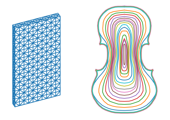
Figure 1. Left: Slab with its triangulation, as used here. Right: Viotti top plate view (without the $f$ holes) and sixteen level sets.

For $\Omega$ the top plate of the Viotti violin without its $f$-holes, the triangulation is more complex. This $\Omega$ can be inscribed into a rectangular box of $35.4\,{\rm cm}\times 20.8\,{\rm cm}$; it is curved with thickness that varies nonuniformly, ranging from a lowest of $0.21$ cm to a largest of $0.36$ cm. In order to obtain a reasonable resolution for this type of thickness and curvature, away from the edge of the plate, we subdivide $\Omega$ into blocks of size $\text{$0.5$ cm}\times\text{$0.5d$ cm}\times\text{$0.5$ cm}$, where $d$ is an average thickness of the plate at points where the block is located. We proceed similarly at the edge, but the first dimension of the blocks we consider there is taken to be nonuniform, out of necessity. All together, it takes 4,608 of these blocks to fill $\Omega$, and the triangulation $K$ that we then derive contains 7,296 vertices, 35,283 edges, 51,028 faces, and 23,040 tetrahedrons; $5,118$ of the vertices, $15,348$ of the edges, and 10,232 of the faces, are on the boundary. The first barycentric subdivision of this triangulation has 116,647 vertices, 699,294 edges, 1,135,608 faces, and 552,960 tetrahedrons; $30,698$ of the vertices, $92,088$ of the edges, and 61,392 of the faces, are located on the boundary. The system (46) has now $1,834,902$ equations in $1,834,902$ unknowns, again, an increase of $62\%$ in size of the corresponding system in [24] (the agreement in the increase between this body and the slab is due to the comparable aspect ratios of their geometries and triangulating elements).

All of these $\Omega$s are topologically $3$d balls with a $2$d sphere boundary. The number of elements in their triangulations $K$ and $K^{\prime}$ satisfy the combinatorial Euler characteristic identity of the $3$d ball, and the number of boundary elements satisfy the combinatorial Euler characteristic identity of the $2$d sphere.

In either case, as we traverse the body across the two blocks separating the bounding surface in the thin direction, the barycentric triangulations used contain 444 faces, with 35 intermediate faces separating pair of boundary faces on opposite ends, which when included yield a total 37 faces altogether traversed in going from one side to the other. These two blocks contain $382$ edges, so there are just about $32$ edges in between the two said faces, and so in going from one side to the other in the thin direction, we cross nearly $69$ triangulation elements that are involved in the expansion of the discretized approximate solution $U$. This provides an adequate resolution for the numerical approximation to accurately capture the true nature of the vibrating wave in these regions, and to propagate in all transversal directions it goes, or feel the propagating waves that are passing by. Refinements of the triangulations would increase the number of elements in going from side to side, and improve the accuracy of the numerical solution $U$, but such would lead to a complexity that is out of the scope of the author’s current computational resources.

As for the additional local boundary conditions that are satisfied by the fine vibration waves approximations, of all the $2\times 6$ subblocks of (41) that the faces in ${{\mathcal{F}}}_{\partial}$ generate, of the 1,040 of them for the slab, exactly eleven have rank one, and of the 10,232 of them for the Viotti plate, exactly one has this property [24]. As pointed out in [24], the differences between the numbers of null rows in the system (41) for the slab and Viotti plate reflect the ${\mathbb{Z}}/2\times{\mathbb{Z}}/2\times{\mathbb{Z}}/2$ symmetry of the triangulation of the former, as opposed to the nonsymmetric nature of the triangulation of the latter, whose thickness varies in a nonuniform manner throughout the body. Notice that the exterior normal to a boundary face, and its normal as an oriented two simplex, are not necessarily the same.

We find the matrices $I$ and $K$ of the systems (46), (48), by executing python code written for this purpose. The code is structured into four major modules. The first two are common to all geometries and topologies, and the last two are body specific, dealing with the coarse and fine waves, respectively. (We have improved the object-oriented conception used in [24], the organization of the code making it straightforward the incorporation of bodies with other physical and topological properties by a mere insertion of the new appropriate modules in the right places.) The processing of the results, and their graphical display, is carried out by some additional python code written for the purpose, the graphical component of it built on top of the PyLab standard library module.

We executed the code on a 2.4GHz Intel Core i7 processor, with 8GB 1600 MHz of memory. The generation of the new blocks in $I$ and $K$ associated to edges only require a CPU time that is of the same order as that taken to generate the blocks corresponding to faces only, reported in [24]. For the number of elements involved, as well as the sparsity of the blocks for edges, are of the same order of magnitude as those for the faces. The hardest new part arises when generating the cross block corresponding to interior edges and interior faces, given the number of elements involved, and the lower sparsity that this off-diagonal subblock has in relation to the others (for the Viotti plate, the sparsity score of the $I_{\circ,\partial}$ matrix of the system (46) here was $0.999990$; in contrast, the sparsity score of the corresponding matrix in [24] was $0.999994$). Overall, the hardware used handles well the complexities of the problem, but the size of it for the Viotti plate already demands the generation of the matrices in stages, parallelizing the calculations on the basis of the linear ordering of the simplices in $K^{\prime}$, and finding them employing a still reasonable amount of CPU time. A true technological problem arises in the calculation of the eigenvectors of (46) and (48) for this plate, which with the eigsh ARPACK routine we use for the purpose, requires the use of a bigger serial system than any we have had available to us (see §6.3.1 below).

The effective cross sectional area of the Viotti plate is about $2.88$ times the effective cross sectional area of the slab, and this produces a difference of one order of magnitude in the number of elements, edges and faces, that we must use in treating one or the other. Should we need to treat a thin $\Omega$ with cross sectional area $2.88$ times larger than that of the Viotti plate, the processor(s) needed for the purpose should be capable of handling matrices of size $10^{7}\times 10^{7}$, which is well within the reach of today’s computers. Our method scales, and thus, seems suitable for the treatment of several imaginable problems of interest in the current technological environment.

6.2. Elastic constants

The components of the tensor of elastic constants $W$ in (24) are those given in (28). For this tensor $W$, the constants $l_{1},l_{2},l_{3}$ in the weighted divergence (44) are

$$\begin{array}[]{rcl}l_{1}&=&1.932758876\cdot 10^{9}\,,\\ l_{2}&=&1.488135884\cdot 10^{9}\,,\\ l_{3}&=&5.884378014\cdot 10^{9}\,.\end{array}$$

As indicated earlier, we take $\rho=360{\rm kg/m^{3}}$, and $\lambda_{L}=1$. These are the values of the constants used in our simulations. The density value implies that the masses of the slabs are $18$g, $9$g, and $4.5$g in decreasing order of their thickness, respectively, and that the mass of the Viotti plate is approximately $59.1$g, very close to the actual mass of many violin plates of this size currently in existence (the Messiah, for instance). Just for the the perspective of the reader, we observe that the density of aluminum, $2,700$ ${\rm kg/m^{3}}$, is $7.5$ times $\rho$.

6.3. Simulations

We analyze first the divergences of the eigenvector wave modes of the systems (46) and (48), respectively, and then do the analysis of the resonance waves that they produce.

6.3.1. The divergence of the coarse and fine normalized eigenvector solutions

The eigenvalues and eigenvectors of the homogeneous systems associated to (46) and (48) are generated using the ARPACK routine eigsh in shift-invert mode, with their corresponding matrix parameters $\rho I$, and $K$, respectively. This computes the solutions $(\lambda,c)$ of the system

$$\rho Ic=\lambda Kc\,.$$

With sigma=-1/(2 pi f)^2, and which=’LM’ passed onto eigsh, we execute the routine for a frequency f any of $80$, $147$, $222$, $304$, and $349$ Hz, respectively. In each case, the routine returns pairs -((2 \pi f_r)^2, c^{f_r}) of eigenvalue and eigenvector of $(\rho I)^{-1}K$, where f_r is the eigenvalue of the matrix closest to the inputted f, in magnitude. We then consider the corresponding normalized eigenvector wave solution for each, the coarse, and fine systems, respectively.

For the Viotti plate simulations, the execution of $\verb+eigsh+$ above to find the eigenvectors fails with the error Can’t expand MemType 1: jcol 1801648, barely missing the end. It is for this reason that we adjust these simulations to use only the face elements in the triangulation, and the corresponding altered equation. These are the results we present below for the Viotti plate. Notice that the altered equation is not the same as that considered in [24], because the definition of the matrix $K$ here differs from what it was then.

In the case of (46), we denote by $f_{coarse}^{r}$ and $c_{s}^{f^{r}_{coarse}}$ the pair (f_r,c^{f_r}) produced for the inputted f, and let

$$U_{f^{f}_{coarse}}=e^{2\pi f^{r}_{coarse}ti}\sum_{W_{s}\in{\mathcal{B}}_{L^{2}_{1}(K^{\prime};{\mathbb{R}}^{3})}}c^{f^{r}_{coarse}}_{s}W_{s}$$

be the normalized coarse eigenvector solution in $L^{2}_{1}(K^{\prime};{\mathbb{R}}^{3})$ that results. In the case of the system (48), we proceed likewise, and let

$$U_{f^{f}_{fine}}=e^{2\pi f^{r}_{fine}ti}\sum_{W_{s}\in{\mathcal{B}}_{L^{2}_{1,b}(K^{\prime};{\mathbb{R}}^{3})}}c^{f^{r}_{fine}}_{s}W_{s}$$

be the normalized fine eigenvector solution in $L^{2}_{1,b}(K^{\prime};{\mathbb{R}}^{3})$ that results from the returned pair (f_r,c^{f_r}) for the given f.

We study the divergence of any of these normalized eigenvector solutions $U$ by computing the flux

$$\int_{\partial\Omega}U\cdot n\,d\sigma$$

through the boundary of the body at time $t=0$. The results are displayed in Table 3.

Body	$f$	$f^{r}_{coarse}$333	flux $U_{f^{f}_{coarse}}$	$f^{r}_{fine}$333	flux $U_{f^{f}_{fine}}$
Slab 1.0	80	79.98300620	-0.0000249730	80.01751279	0.0000009708
	147	146.90402861	-0.0001222083	146.01597845	0.0000663559
	222	221.93558743	0.0003161676	220.45892181	-0.0057717711
	304	304.03517536	-0.0023043236	304.01774121	-0.0000023969
	349	348.94594451	-0.0000171669	348.96922189	0.0000051104
Slab 0.5	80	79.44465641	-0.0041503791	79.44465959	-0.0009114188
	147	145.97955476	-0.0083605924	145.97955400	-0.0020807749
	222	220.45898203	-0.0026676193	220.46140952	-0.0002427300
	304	301.88969619	-0.0076778693	301.88974794	-0.0016486990
	349	349.09691350	-0.0000202374	349.05496747	-0.0000142132
Slab 0.25	80	79.44465624	-0.0031694079	79.44465547	-0.0063644096
	147	145.97955476	-0.0059265938	145.97955448	-0.0063411167
	222	220.45898620	-0.0018536358	221.99574371	0.0000703494
	304	301.88969891	-0.0050515305	301.88969505	-0.0041960055
	349	348.90773121	-0.0000748571	349.09787762	0.0000857175
Viotti plate	80	79.99818471	-0.0087776487	79.99972869	-0.0070498420
	147	146.99513939	-0.0168672080	146.99453429	0.0173401990
	222	222.00259999	0.0112724697	221.99478910	-0.0005874142
	304	303.99865189	-0.0053818663	304.00167789	-0.0094033063
	349	348.99889409	-0.0036936708	349.00660655	0.0029127309

Table 3. Initial fluxes for the coarse and fine eigenvector solutions. The results for the Viotti plate are derived using the face elements only.

We repeat this experiment just for the slab of depth $0.5$cm using the value $\lambda_{L}=3.101757591\cdot 10^{9}$, the average of $l_{1}$, $l_{2}$, and $l_{3}$ above, instead of $1$. Then, the spatial terms in equation (38), which are all of order two, have coefficients that are of the same order of magnitude, and for certain frequencies, the modifying weak term $-\lambda_{L}\langle{\rm div}\,u,{\rm div}\,u\rangle$ could drag the other two microlocally towards an operator that is not elliptic, producing a non physical wave result that could be detected by some numerical inconsistency, for instance, a negative “norm” for the eigenmode that is to be normalized in order to compute its flux. This does not happen here at any of the five frequencies used in our simulations, but could in principle occur for others that remain unexplored. The complete results are displayed in Table 4.

	$f$	$f^{r}_{coarse}$333	flux $U_{f^{f}_{coarse}}$	$f^{r}_{fine}$333	flux $U_{f^{f}_{fine}}$
$\begin{array}[]{c}\text{Slab 0.5}\\ \lambda_{L}=3.1\cdot 10^{9}\end{array}$	80	79.44465548	0.0085159297	79.44465548	0.0172430719
	147	146.91260194	0.0001067346	145.97955453	0.0188712978
	222	222.22211502	-0.0000724956	220.45891928	-0.0196273836
	304	301.88969256	-0.0080961614	301.88969160	0.0256947693
	349	346.57731074	-0.0082506915	346.57731061	-0.0316121099

Table 4. Slab 05: Initial fluxes for the coarse and fine eigenvector solutions of the equation with $\lambda_{L}=3.101757591\cdot 10^{9}$.

6.3.2. Coarse and fine resonance waves

We subject the body to an external sinusoidal pressure wave of the form

$$\vec{F}^{ext}=\vec{F}_{0}\sin({\bf k}\cdot{\bf x}\mp\omega t)=\vec{F}_{0}\sin({\bf k}\cdot{\bf x})\cos({\omega t})\mp\vec{F}_{0}\cos({\bf k}\cdot{\bf x})\sin({\omega t})$$

that travels in the appropriate direction for it to hit the bottom of the slab, or belly of the Viotti plate, first. If $k=|{\bf k}|$ is the magnitude of the wave vector, we use $v=\omega/k=343$ m/sec, the speed of sound in dry air at $20\mbox{}^{\circ}$C. The source of the wave is placed at a distance of $62$cm from the body, along a line that passes through the height-width plane of the body perpendicularly at the half way point of both, its height and width. This external force $\vec{F}^{ext}$ induces a force on the body, which we denote by $\vec{F}_{\omega}$.

The coarse (46) and fine (48) systems are considered with the nonhomogeneous force term $F=\vec{F}_{\omega}$, and with trivial initial data. (These are the coarse and fine discrete versions of the initial value problem for (16) when this system is viewed as the second order equation (38).) The nonhomogeneous terms in these systems are vectors of the form

$$\vec{C}_{1}\cos{(\omega t)}\mp\vec{C}_{2}\sin{(\omega t)}\,,$$

where $\vec{C}_{1}$ and $\vec{C}_{2}$ are time independent vector fields on the body. If $\omega=2\pi f$ for $f$ any of the frequency values $80$, $147$, $222$, $304$, and $349$ Hz, respectively, we let $\omega_{f_{r}}=2\pi f_{r}$ be the closest eigenvalue to $\omega$ that the matrix $(\rho I)^{-1}K$ has, $\rho I$ and $K$ the matrices of the system in consideration. The resonance wave that this vibration mode produces is given by

(55) $$W_{f_{r}}=\frac{1}{\omega^{2}_{f_{r}}-\omega^{2}}\sum_{W_{s}}\left(c^{W_{s}}_{1}\left(-\cos{(\omega_{f_{r}}t)}+\cos{(\omega t)}\right)\pm c^{W_{s}}_{2}\left(\frac{\omega}{\omega_{f_{r}}}\sin{(\omega_{f_{r}}t)}-\sin{(\omega t)}\right)\right)W_{s}\,,$$

where, for each $j=1,2$, the vector $\vec{c}_{j}=(c_{j}^{W_{s}})$ is the solution to the linear system of equations

$$-((2\pi f)^{2}\rho I+K)\vec{c}_{j}=\vec{C}_{j}\,.$$

The summation is over the basis elements $W_{s}$ of $L^{2}_{1}(K^{\prime};{\mathbb{R}}^{3})$ and $L^{2}_{1,b}(K^{\prime};{\mathbb{R}}^{3})$ for the coarse and fine systems, respectively.

We generate the vector $\vec{C}_{j}$ as a function of $\vec{F}_{\omega}$, and the geometry of the body, and then solve the system of equations above for $\vec{c}_{j}$ using the scipy.sparse.linalg routine spsolve, with the appropriate parameters.

We compute the values of the resonance wave at the barycenter, and vertices, of the boundary faces on the side of the body opposite to the incoming external wave $\vec{F}^{ext}$. There are $3,661$ such points for the slabs, and $42,069$ for the Viotti plate. We do these calculations at the equally spaced times $t_{j}=j\frac{2\pi}{10\omega}$, $j=1,\ldots,10$, corresponding to a full cycle of the external wave. For each $t_{j}$, we find the maximum ${\rm max}_{t_{j}}=\max{\{\|W_{f_{r}}(t_{j})\|}\}$ and minimum ${\rm min}_{t_{j}}=\min{\{\|W_{f_{r}}(t_{j})}\|\}$ of the set of norms of the resonance wave at the indicated points, and with $\delta_{t_{j}}=\frac{1}{10}({\rm max}_{t_{j}}-{\rm min}_{t_{j}})$, any of the said points is considered to be nodal at time $t_{j}$ if the norm of the resonance wave solution at the point is no larger than ${\rm min}_{t_{j}}+c_{\Omega}\delta_{t_{j}}$, with $c_{\Omega}=0.05$ for the slabs, and $c_{\Omega}=0.00002$ for the Viotti plate, respectively. We then declare a point to be nodal if it is nodal at all the $t_{j}$s. These are the points that we display.

The results for the coarse and fine resonance waves are depicted in Figs. 2-5 below. In each case, we indicate the value of $c_{\Omega}$ that is being used to define a point as nodal.

The triangulations with simplices of best aspect ratios are those for the slab of depth $1$cm, and the Viotti plate. We restrict our attention to them, and study the change in the resulting resonance pattern produced by taking into consideration now the six modes with eigenvalues $\omega_{f_{r_{j}}}=2\pi f_{r_{j}}$, $j=1,\ldots,6$, closest to $\omega=2\pi f$, as opposed to the single closest one, as above. The resonance wave is then a sum of six terms as in (55), one per each of the $f_{r_{j}}$s. We show the results of these simulation for the slab plate resonating at the frequency $f=147$Hz only, Fig. 6. The five cases depicted correspond to nodal points defined as above for values of $c_{\Omega}=0.1,0.05,0.03,0.02$, and $0.005$, respectively. We bypass showing the corresponding image for the Viotti plate because of the difficulties encountered with eigsh to find its resonance vibration modes using edges and faces together. The image we obtain using the face elements only compares very well to its analogue [24, Figure 7], the equation solved here being better when studying the resonance patterns over a wider range of vibrations, not just the small ones back then.

Finally, we look at the divergence of the resonance waves above. We denote by $W_{f_{coarse}^{f}}$ and $W_{f_{fine}^{f}}$ the normalized coarse and fine resonance wave solutions associated to the pair $(f,f_{r})$ for (46), and (48), respectively. As these waves start with trivial initial conditions, we quantify the extent to which our algorithm maintains the divergence free condition on them throughout time by evaluating their fluxes over the boundary at the time $t_{j}$, in each case, where the quotient ${\rm max}_{t_{j}}/{\rm min}_{t_{j}}$ is the largest. The normalization performed on the resonance waves makes the results independent of the magnitude of $\vec{F}_{0}$ in the external wave $\vec{F}^{ext}$ that induces the resonance. The said $t_{j}$ (at which value the fluxes are being evaluated) turns out to be a nontrivial function of $\Omega$ and $f$, as opposed to the analogous situation in [24], where it was equal to $t_{7}$ always. The results are listed in Table 5.

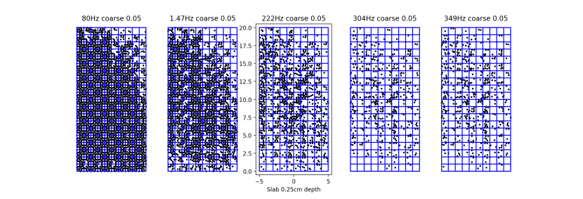
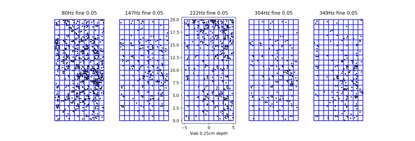
Figure 2. Slab $10\times 0.25\times 20$: Nodal points of the resonance waves at $f$Hz arising from the slab mode of vibration of frequency $f_{r}$ closest to $f$. The notion of nodal point is defined by $c_{\Omega}=0.05$.

6.4. Discussion of the results: Validation

The elastic constant values in Tables 1 and 2 for the Engelmann Spruce had been collected from wood with a 12% moisture content [12], which is not very conducive to the creation of good vibration patterns, and although the density value we employ in our simulations is close to the density of actual wood used in the making of violin plates, if compared to the original, our model for the Viotti plate is dull, and vibrates poorly. (D. Caron, a renowned american luthier, makes his violin plates using wood with a moisture content in the range of 2%-5% [4]; this content is lowered when the plate is coated with varnish, which adds mass and absorbs some moisture as it dries. The addition of the varnish changes the flexibility by stiffening the plate across the grain, in effect, creating an almost functionally graded plate, though not isotropic.) In spite of this drawback, the vibration patterns of the bodies in our simulations are very close to what they would be in practice under those nonideal circumstances.

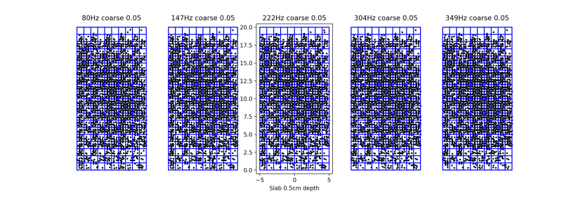
Figure 3. Slab $10\times 0.5\times 20$: Nodal points of the resonance waves at $f$Hz arising from the slab mode of vibration of frequency $f_{r}$ closest to $f$. The notion of nodal point is defined by $c_{\Omega}=0.05$.

Figs. 2-4, and 6 depict resonance patters in remarkable agreement with holographic images of standing sound waves, propagating in a body under experimental conditions comparable to those in our simulations (see, for instance, [20, Figs. 4, 6, 7]), showing that they are what they are supposed to be. The corresponding resonance patterns in Figs. 4 and 6 exhibit just a better definition of the details if we take into consideration the six vibrations modes closest to $147$Hz, as opposed to the single closest one, but not an actual change in the pattern, and in Fig. 6, as the notion of a nodal point becomes stricter by decreasing the value of $c_{\Omega}$, clearer details in the resulting patterns emerge. The simulation at $147$Hz for the Viotti plate in Fig. 5, which is derived using the face elements only, points quite closely towards the image by holographic interferometry of the mode 2 of a top violin plate in [14, Fig. on p. 177], and improves on those shown in [24, Figs. 6, 7]. In spite of the differing conditions between our simulations and the cited holographic experiments, we take the favorable comparison as a validation of our results. We elaborate on a few additional details of our simulations.

Figure 4. Slab $10\times 1.0\times 20$: Nodal points of the resonance waves at $f$Hz arising from the slab mode of vibration of frequency $f_{r}$ closest to $f$. The notion of nodal point is defined by $c_{\Omega}=0.05$.

For the two most geometrically degenerate bodies in our simulations, at a given frequency, the number of nodal points of the coarse waves is larger than the number for the fine waves. As the frequencies increase, the ratios of these numbers are 2.08, 2.15, 2.37, 2.51, and 2.41 for the slab of depth $0.5$cm, and 10.62, 10.88, 3.23, 3.13 and 2.88 for the slab of depth $0.25$cm, respectively. These patterns breaks altogether for the slab of depth 1cm, and for the Viotti plate, the two bodies in our simulations with triangulations of simplices of best aspect ratios. For comparison purposes, the said quotients for the thicker slab are 0.73, 0.71, 1.13, 1.14, and 0.60, while for the Viotti plate they are 0.33, 1.32, 0.49, 0.22, and 1.48, respectively.

A close look at the number of nodal points for the slabs in our simulations indicate a limitation to the effect of selective thinning of the plate, a practice among luthiers that is commonly believed to lower or increase frequency modes if carried out in regions of high or low curvature, respectively. For the thickest of the slabs the number of fine nodal points varies somewhat sinusoidally with $f$, oscillating about 1,990. For the slab of depth $05$cm, the numbers go as 1,076, 1,050, 965, 928, and 945, , while for the thinnest slab they go as 276, 215, 381, 158, and 188, respectively. At some point, the effect of additional thinning acts differently on the various vibration modes, counterbalancing the strength they have relative to each other.

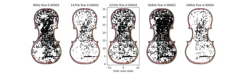
Figure 5. Viotti plate: Nodal points of the resonance waves at $f$Hz arising from the plate mode of vibration of frequency $f_{r}$ closest to $f$ (results derived using the face elements only). The notion of nodal point is defined by $c_{\Omega}=0.00002$.

The curvature of the violin plate is an important factor in the relative magnitude of the amplitude of the resonance wave near $f=349$Hz compared to the amplitude of the resonance wave near $f=80$Hz. The quotient of these amplitudes for the Viotti plate is of the order of $10$, while for the slab of depth $1$cm is of the order of $2\cdot 10^{3}$. (The brightness of this vibration mode is reported to be of importance in prejudging the good quality of an assembled instrument with the plate in it [14].) Of course, the comparison is weak in that the simulation for the Viotti plate was carried out using only the face elements, however many. But the resonance pattern that we have so obtained, Fig. 5, in spite of the poor quality of the wood used, is remarkably good.

7. Concluding remarks: Computational physics merging with computational topology

If $\eta$ is a solution of (2), (3), (4), we have that ${\rm div}_{\eta}\dot{\eta}=0$, and the linearized equations of motion about $(\eta,\dot{\eta})$ have as solution a curve $(u(t),\dot{u}(t))$ with $u$ a divergence-free vector field that, while well-defined, yields a curve in the Abelian group $H^{2}(\Omega;{\mathbb{R}})$. Solving for $u$ then is fraught with the problems inherent to maintaining the closed divergence-free property that the initial condition satisfies, hard theoretically, and harder computationally.

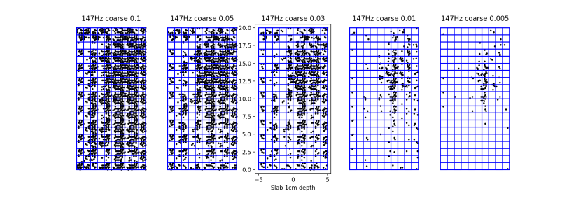
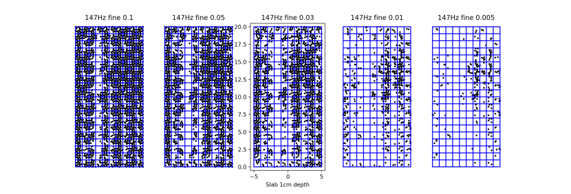
Figure 6. Nodal points of the resonance wave at $f=147$Hz arising from the six closest mode of vibrations of the plate to this frequency $f$. From left to right, the notion of nodal point is defined by $c_{\Omega}=0.1$, $0.05$, $0.03$, $0.01$, and $0.005$, respectively.

The linearized equations about a point $(\eta,\dot{\eta})$ other than $(\eta(t)x=x,0)$ produces an operator that is hyperbolic on the tangent space at $\eta$ of the submanifold defined by (2). The dependence of the space on $\eta$ makes it difficult to prove the well-posedness of its associated Cauchy problem in the usual manner. We enlarge the space to prevent this problem, but this in turn forces us to modify the equation in order to maintain the ellipticity of the spatial part of the linearized operator, and have its hyperbolicity on the larger domain. This is what we accomplish when we modify (5), and look at (7) instead, the latter an equation whose volume preserving solutions solve (5) as well. Technical issues aside, we then show that the fixed point $(\eta,\dot{\eta})$ of the contraction mapping principle that we devise solves the modified equation, and is volume preserving, so this fixed point solves (5) as well, which is what we wanted.

Body	$f$	$f^{r}_{coarse}$333	flux $W_{f^{f}_{coarse}}$	$f^{r}_{fine}$333	flux $W_{f^{f}_{fine}}$
Slab 1.0	80	79.98300620	-0.0045986774	80.01751279	-0.0000092823
	147	146.90402861	-0.0022899377	146.01597845	-0.0000271994
	222	221.93558743	-0.0074495371	220.45892181	-0.0000039583
	304	304.03517536	0.0006411380	304.01774121	0.0000089606
	349	348.94594451	-0.0141437966	348.96922189	0.0000717342
Slab 0.5	80	79.44465641	0.0000233879	79.44465959	0.0000114983
	147	145.97955476	0.0000740003	145.97955400	0.0000103866
	222	220.45898203	0.0001275103	220.46140952	0.0000111290
	304	301.88969619	0.0003156497	301.88974794	0.0000175093
	349	349.09691350	0.0004423489	349.05496747	0.0000111168
Slab 0.25	80	79.44465624	-0.0000157439	79.44465547	0.0000021530
	147	145.97955476	0.0000016388	145.97955448	0.0000103168
	222	220.45898620	-0.0000246448	221.99574371	0.0000710929
	304	301.88969891	0.0002215706	301.88969505	0.0000297836
	349	348.90773121	0.0003536785	349.09787762	-0.0000881610
Viotti plate	80	79.99818471	-0.0189303539	79.99972869	0.0035747785
	147	146.99513939	-0.0575648428	146.99453429	-0.0977355895
	222	222.00259999	-0.0189054794	221.99478910	-0.0118013729
	304	303.99865189	-0.0072224699	304.00167789	0.0000439681
	349	348.99889409	-0.0036936708	349.00660655	-0.0922473868

Table 5. Fluxes of the normalized coarse and fine resonance waves computed each at the value of $t_{j}$ maximizing ${\rm max}_{t_{j}}/{\rm min}_{t_{j}}$ (results for Viotti plate derived using the face elements only).

Having the existence settled, we can then turn our attention to the finding of a good numerical approximation to it. As it is impossible to maintain a closed condition when you solve numerically any equation, we give up on attempting to compute the volume preserving diffeomorphism solution of the equation, and use the iterates of the Newton scheme in the proof of its existence as the candidates to approximate it instead. The velocity fields of the diffeomorphisms in the iteration are not divergence-free per se, but close to one. Such a condition, a matter of satisfying an equation that locally involves finitely many of the coefficients in the discretized unknown, is left to be regulated by the equation itself, and if holding initially, it should be satisfied at later times within a small margin of error also due to the well-posedness of the problem solved, thus ensuring that the nonlocal incompressible condition of the diffeomorphism solution stays within a striking level of tolerance. Thus, we can accurately captured it numerically if we use discretizing spaces for them that are natural relative to the complexities of the problem, and that encode into them the algebraic topology of the actual solution velocity curve in the cohomology group above that this velocity represents, a global property. This is where we enter a triangulation $K$ of $\Omega$, and all of the Whitney forms of the simplices of its barycentric subdivision $K^{\prime}$. Through them we resolve both of these last issues in earnest.

For any $k$, $0\leq k\leq n$, the Whitney forms of the simplices in $K^{\prime}$ of degree $k$ are a finite basis of the $k$th cochain group of $K^{\prime}$. Since the simplices are all contractible, we may define locally a notion of $*$ operator, and use the $*$ of the Whitney forms of degree $n-k$ simplices to generate a dual cochain group of $k$-simplices in $K^{\prime}$. Preserving its algebraic topology properties, we discretize any $k$-form in the direct sum of these two groups, a set-up that is closely related to the dual block decomposition of $K^{\prime}$, and the proof of the Poincaré duality $H^{n-k}(K^{\prime};{\mathbb{R}})\cong H_{k}(K^{\prime};{\mathbb{R}})$. Using the individual groups for this purpose would lead to the loss of algebraic topology information, although some is still preserved. With that resolved, the issue of a proper resolution for an accurate numerical approximation of the said $k$-form is addressed by controlling the aspect ratios of all the simplices in $K$, making of this a relatively uniform number throughout the entire polytope $|K|$. A minimum lower bound on this number ensures a resolution good enough to have the form accurately described by its numerical approximation. This is what we have done in our problem, where $n=3$, and $k=1$, except for the additional fact that instead of looking at the $k$ form, we have worked equivalently with its metric dual vector field.

The large systems of equations that need to be solved, however sparse, are computationally challenging, and this is a difficulty that we must face even after resolving that of determining the systems themselves. The judicious choice of discretizing spaces minimizes these difficulties. Since we encode in them the initial conditions of the waves we seek, with the algebraic topological properties that they have, we can then allow the well-posedness of the equations solved for to play its role in keeping the numerical solutions derived physically accurate in time.

The use of Whitney forms associated to edges for numerical purposes of sort is well established already [19, 1, 2], but often they have been employed to discretize physical quantities that truly represent cohomology classes in degree two, rather than one, and for which the use of the Whitney forms associated to faces would be more natural instead [24], the direct sum of the forms for edges and faces described here a better candidate to work with, as a discretizing space, in general. Historically, as computers started to be developed, functions were approximated by their values at finitely many points chosen uniformly over their domains, the number of these points limited by the memory capacity, rather than expanding them as linear combinations of the elements in the partition of unity given by the Whitney forms associated to vertices, or tetrahedrons, individually, or together as a direct sum. That to a great extent this has remained so is kind of surprising, given the common use of orthonormal basis of $L^{2}$ functions derived from a starting wavelet [5, 6, 17], and which has appeared frequently in the numerical analysis of signals in a noisy background, the orthonormality of the basis ensuring that in the representation of the sequence of images as a discrete set of observation processes, the noise is no more correlated than it was in the original images [13]. The space ${\rm Char}(K^{\prime})$ serves perfectly well in that capacity also, an orthogonal partition of unity basis of $L^{2}$ functions generated by the Haar wavelet supported on a model top dimensional simplex. But the sum ${\rm Fun}(K^{\prime})\oplus{\rm Char}(K^{\prime})$ would be better for general purposes, as we had seen in §4, the natural space to discretize functions as a sum of their components in the image of the Laplace operator, and their orthogonal complements.

Regardless, the use of these forms is being increasingly advocated today in numerical analysis [3], and have regained some of the momentum they had at the time of Whitney (who had used them for several “computations” already), and shortly thereafter [8]. If their properties are exploited well, they serve to capture the essential algebraic structure underlying the problems under consideration, and, with a minimal number of computational elements, we may use that fact to derive accurate approximations of solutions to problems with large intrinsic complexities. The geometric content of a triangulation is a powerful tool to use to compute polytope quantities of physical significance [11], a tool through which we may control the local geometry of the problem. But the power of this tool truly comes to fruition if we include in the considerations its algebraic content as well, since then we can use it to tie up, and control, both the local, and global geometric and topological properties of it. The serial computer power remains a hindrance only to the size of the problem that you can treat, but that is just a technological issue. Parallelizing the calculations will take you as far as that may go, but if and when you need to proceed to do so, you know beforehand that the problem you are solving for is well posed.

As we indicated earlier, we can also study the vibrational patterns of elastic bodies with corners, under mild assumptions on their stored energy functions, or even bodies where part of the boundary is fixed while the rest is free to move. These are all variations of the theme treated here. What is of more importance is the fact that the computation of any time evolving tensor of physical significance can be treated in this manner also. We just need to add a minor part to the set-up above concerning the Whitney forms. For a simplex $\sigma_{k}=[x_{p_{0}},x_{p_{1}},\ldots,x_{p_{k}}]$, the Whitney form associated to it is the complete alternation of the tensor $\tau_{\sigma_{k}}=x_{p_{0}}dx_{p_{1}}\otimes\cdots\otimes dx_{p_{k}}$. In general, in order to treat evolving tensors that are not purely contravariant in a manner similar to the treatment of the tensor in our problem here, we would have to use the complete symmetrization of all the $\tau_{\sigma_{k}}$s as well, in parallel with the use of all of the Whitney forms, as above. The collection of all of these local elements associated to the simplices of $K^{\prime}$ is the optimal space where to track, at the discrete level, a weak version of the tensor.

References

• [1] J.S. Asvestas, B. Bielefeld, Y. Deng, J. Glimm, S. Simanca & F. Tangerman, Electromagnetic scattering from large cavities: Iterative methods, Comm. Appl. Anal. 2 (1998), pp. 37-47.
• [2] A. Bossavit, A new rationale for edge-elements, Int. Compumag Soc. Newslett. 1 (1995) pp. 3–6.
• [3] A. Bossavit & F. Rapetti, Whitney forms of higher degree, SIAM J. Numer. Anal. 47 (2009) pp. 2369-2386.
• [4] D. Caron, Private communication. (2018) Taos, NM.
• [5] I. Daubechies, The wavelet transform, time-frequency localization, and signal analysis, IEEE Trans. Information Theory, 36 (1990), pp. 961- 1,005.
• [6] I. Daubechies, Orthonormal basis of compactly supported wavelets, Comm. Pure Appl. Math., 41 (1988), pp. 909-996.
• [7] J. Dilworth, Stradivari ‘Viotti’ violin 1709 poster. The Strad Library.
• [8] J. Dodziuk, Finite-difference approach to the Hodge theory of harmonic forms, Amer. J. Math. 98 (1976), pp. 79-104.
• [9] D.G. Ebin & S.R. Simanca, Small Deformations of Incompressible Bodies with Free Boundary. Comm. in P.D.E., 15 (1990), pp. 1588-1617,
• [10] D.G. Ebin & S.R. Simanca, Deformations of Incompressible Bodies with Free Boundary. Arch. Rational Mech. Anal., 120 (1992), pp. 61-97.
• [11] J. Glimm, S.R. Simanca, T. Smith & F. Tangerman, Computational Physics meets Computational Geometry, preprint (1996), available at ftp://ftp.ams.sunysb.edu/papers/1996/susb96_19.ps.gz.
• [12] D. Green, J. Winandy & D. Kretschmann, Mechanical properties of wood, Wood handbook: wood as an engineering material. Madison, WI: USDA Forest Service, Forest Products Laboratory, 1999. GTR-113: Pages 4.1-4.45
• [13] Z. Haddad & S.R. Simanca, Filtering Imaging Records Using Wavelets and the Zakai Equation, IEEE Trans. PAMI 17 (1995), no. 11, pp. 1069-1078.
• [14] C.M. Hutchins, The Acoustics of Violin Plates, Scientific American, 245 (1981), pp. 171-186.
• [15] J.L. Lions & E. Magenes, Non-homogeneous boundary value problems and applications, Vol. I. Translated from the French by P. Kenneth. Die Grundlehren der mathematischen Wissenschaften, Band 181. Springer-Verlag, New York-Heidelberg, 1972. xvi+357 pp.
• [16] A. Mahi, E.A.A. Bedia & A. Tounsi, A new hyperbolic shear deformation theory for bending and free vibration analysis of isotropic, functionally graded, sandwich and laminated composite plates, Appl. Math. Mod. 39 (2015), pp. 2489-2508.
• [17] S. Mallat, A compact multiresolution representation: The wavelet model, Proc. IEEE Workshop Computer Vision (1987), pp. 2-7.
• [18] J.R. Munkres, Elements of algebraic topology. Addison-Wesley Publishing Company, Menlo Park, CA, 1984. ix+454 pp.
• [19] S.M. Rao, D.R. Wilton, & A.W. Glisson, Electromagnetic scattering by surfaces of arbitrary shape, IEEE Trans. Antennas and Propagation, 3 (1982), pp. 409-418.
• [20] D.A. Russell, D.E. Parker & R.S. Hughes, Analysis of standing sound waves using holographic interferometry, Am. J. Phys. 77 (2009), pp. 678-682.
• [21] S.R. Simanca, Mixed elliptic boundary value problems. Comm. Partial Differential Equations 12 (1987), pp. 123–200.
• [22] S.R. Simanca, Pseudo-differential Operators. Pitman Research Notes in Mathematics Series, 236. Longman Scientific & Technical, Harlow; copublished in the United States with John Wiley & Sons, Inc., New York, 1990. 123 pp.
• [23] S.R. Simanca, Riemannian metric representatives of the Stiefel-Whitney classes, preprint 2020, arXiv:2004.05719.
• [24] S.R. Simanca, The (small) vibrations of thin plates, Nonlinearity, 32 (2019), pp. 1175-1205.
• [25] H. Whitney, Geometric Integration Theory, Princeton University Press, 1957.