Bansak and Paulson

Dynamic Refugee Assignment

Outcome-Driven Dynamic Refugee Assignment with Allocation Balancing

Kirk Bansak Department of Political Science, University of California, San Diego, kbansak@ucsd.edu Elisabeth Paulson Immigration Policy Lab, Stanford University and the Technology and Operations Management Unit, Harvard Business School, epaulson@stanford.edu

This study proposes two new dynamic assignment algorithms to match refugees and asylum seekers to geographic localities within a host country. The first, currently implemented in a multi-year pilot in Switzerland, seeks to maximize the average predicted employment level (or any measured outcome of interest) of refugees through a minimum-discord online assignment algorithm. Although the proposed algorithm achieves near-optimal expected employment compared to the hindsight-optimal solution (and improves upon the status quo procedure by about 40%), it results in a periodically imbalanced allocation to the localities over time. This leads to undesirable workload inefficiencies for resettlement resources and agents. To address this problem, the second algorithm balances the goal of improving refugee outcomes with the desire for an even allocation over time. The performance of the proposed methods is illustrated using real refugee resettlement data from a large resettlement agency in the United States. On this dataset, we find that the allocation balancing algorithm can achieve near-perfect balance over time with only a small loss in expected employment compared to the pure employment-maximizing algorithm. In addition, the allocation balancing algorithm offers a number of ancillary benefits compared to pure outcome-maximization, including robustness to unknown arrival flows and greater exploration.

dynamic assignment algorithms, stochastic programming, load balancing, refugee matching, machine learning

1 Introduction

Host countries have, in recent years, been faced with increasing flows of refugees and asylum seekers. Currently, the United Nations Refugee Agency estimates that there are over 26 million refugees worldwide (United Nations 2020). In most countries that accept refugees and/or asylum seekers, refugees and asylum seekers are assigned and relocated (at least on a preliminary basis) across various localities by migration authorities. The capacity quotas or target distributions of refugees across the localities are determined by authorities on a yearly or other regular basis. Increasing inflows pose a strain on host countries, whose goal is to help these new arrivals achieve economic self-sufficiency and other positive integration outcomes. Accordingly, a number of countries have begun to explore and implement outcome-based geographic matching in their refugee resettlement and/or asylum programs. Therefore, recent research studies the problem of efficiently assigning refugees to localities in order to maximize outcomes such as employment (Bansak et al. 2018, Trapp et al. 2018). This research falls within a broader area of policy interest as national resettlement programs seek new approaches to help ever-increasing flows of refugees and asylum seekers better integrate (e.g. find employment) in their host countries (e.g. Mousa 2018, Andersson et al. 2018, Gölz and Procaccia 2019, Olberg and Seuken 2019, Acharya et al. 2021, Ahani et al. 2021).

Outcome-based matching was introduced in the context of refugee and asylum-seeker assignment by Bansak et al. (2018), with the goal of leveraging administrative data to improve key refugee outcomes (e.g. employment in the host country) by optimizing refugees’ geographic assignment within a country. To do so, machine learning methods are used to predict refugees’ expected outcomes in each possible landing location as a function of the refugees’ personal characteristics. Those expected outcomes are then used as inputs into constrained optimal matching procedures to determine a location recommendation for each refugee. Since its proposal, outcome-based matching has been piloted by the Swiss State Secretariat of Migration (SEM) in collaboration with the Bansak et al. (2018) research team, and by HIAS (a resettlement agency in the United States) in collaboration with Trapp et al. (2018), with future interest expressed by other countries and agencies as well.

A greedy approach to the refugee assignment problem—one that assigns each refugee to the location with the highest predicted outcome—is suboptimal because of the capacity constraints of the locations. Namely, each location only has a certain number of slots in a given time period (for the United States, the time period is one year, but this can vary across host countries). Therefore, Bansak et al. (2018) and other previous studies on outcome-based refugee matching (e.g. Trapp et al. 2018, Gölz and Procaccia 2019) have proposed optimal matching approaches to the refugee assignment problem that takes into account these capacity constraints.

This paper, along with the concurrent work of Ahani et al. (2021), is the first to consider the dynamic aspect of the outcome-maximization matching problem. In many countries—including the United States (US), Switzerland, Sweden, the Netherlands, and Norway—refugees and asylum seekers must be assigned to a locality virtually immediately upon being processed by resettlement authorities. As a result, each arriving refugee or asylum seeker case (an individual or family) is typically assigned in an online fashion, and these assignments cannot be reversed. The dynamic aspect of this problem introduces a key trade-off between immediate and future rewards: assigning a current case to a location results in an immediate reward (namely, the employment score of the current case at that location), but also uses up a slot at that location for future arrivals.

The goal of this paper is to develop a new assignment algorithm that dynamically matches refugees and asylum seekers to localities within host countries in order to improve employment outcomes while maintaining a smooth balance on the load placed over time on the receiving localities—which include burdens placed on local communities, service providers, and resettlement agents. This paper introduces two new dynamic matching algorithms. The first is a “minimum-discord” outcome-maximization algorithm that seeks to maximize the refugees’ expected employment (or any alternative outcome of interest), and is currently employed in a three-year pilot implementation in Switzerland, undertaken by the Swiss State Secretariat of Migration in collaboration with academic researchers (see Bansak et al. 2018). The proposed algorithm is a special case of the Bayes Selector algorithm introduced by Vera and Banerjee (2020), whose goal is to minimize the likelihood that the online algorithm makes a decision that conflicts with an offline benchmark in each time period.

The second algorithm proposed in this paper is an extension that integrates principles of load balancing into the objective. Because each locality has a given amount of resources (e.g. number of resettlement officers) that cannot be transferred across localities, maintaining a steady workload is crucial and is a first-order concern of many host countries. Hence, building on the minimum-discord outcome-maximization algorithm and borrowing ideas from queuing theory, the second algorithm incorporates wait time minimization into the assignment process. This allows refugees to be dynamically assigned to localities in a way that improves their expected employment scores while also maintaining a balanced allocation across the localities over time.

This paper focuses on the US context, although the methods presented can be readily applied within other host countries, and are currently employed in a pilot program in Switzerland. The performance of the proposed algorithms is demonstrated on real refugee resettlement data from one of the largest resettlement agencies in the US. We find that the minimum-discord outcome-maximizing algorithm achieves near-optimal employment compared to the hindsight-optimal solution. However, this algorithm results in significant imbalance at the localities over time. Modeling each locality as a single server queue, imbalance is measured through the total wait time and idle time at each location. The allocation balancing algorithm is able to drastically decrease both wait time and idle time with surprisingly little loss in employment.

Finally, the allocation balancing algorithm also offers several ancillary benefits. In particular, the balancing algorithm provides an immediate solution to the issue of an unknown total number of arrivals. For example, when the final number of arriving refugees or asylum seekers ends up being lower than initial plans/projections, the final allocation could end up being far from the desired year-end allocation proportions, as quotas will be filled for certain localities but not others. In smoothing the allocation across localities over time, the balancing algorithm averts this problem. As an additional benefit, the balancing algorithm also helps to improve the resilience of the underlying learning system through greater exploration.

1.1 Contributions

1. Minimum-discord outcome-maximizing dynamic assignment algorithm. We propose a “minimum-discord” online algorithm that assigns arriving refugees to locations within a host country. The goal of the algorithm is to maximize the sum of individual outcomes along a horizon, while obeying the capacity constraints of each location. This is accomplished through a Monte-Carlo-sampling-based method that seeks to minimize the probability of choosing the “wrong” assignment in each time period compared to an offline benchmark. This is referred to as a “minimum-discord” approach. The proposed method not only achieves near-optimal performance compared to the hindsight-optimal solution, but is also readily explainable—a desirable property in policy settings.

2. Allocation balancing dynamic assignment algorithm. We demonstrate that an outcome-maximizing assignment (not only online algorithms but even a hypothetical implementation of the hindsight-optimal solution) can result in severe periodic imbalance across the localities over time. Thus, we develop a second online algorithm that explicitly balances the trade-off between outcomes and wait time at the localities using a single parameter, $\gamma$, that controls the weight placed on allocation balancing. Larger values of $\gamma$ result in greater balance (less wait time and idle time).

3. Results on real US refugee resettlement data. The results of the proposed methods are tested on real refugee resettlement data from one of the largest resettlement agencies in the US. Using the cases that arrived in 2016 as our test cohort, the minimum-discord outcome-maximizing algorithm achieves 95% of the hindsight-optimal employment. The 5% optimality gap is primarily due to non-stationarity in the true arrival process. When the arrival dates of the cases are randomly perturbed to mimic a stationary process, the optimality percentage of the proposed algorithm increases to 99.5%. The performance of our algorithm is compared to the employment achieved under the actual historical assignments, as well as greedy and random assignment baselines, which achieve 69%, 81%, and 67% of the hindsight-optimal employment, respectively.

   Using the allocation balancing algorithm, we demonstrate the trade-off between total employment and wait time as $\gamma$ varies. As an example, for a particular choice of $\gamma$, the allocation balancing algorithm is able to significantly reduce wait time (by 88%) and idle time (by 76%) with only a 2% decrease in employment.

1.2 Related Literature

This paper is related to the existing literature on refugee assignment, online stochastic bipartite matching, one-sided matching with queues, and load balancing. In what follows, we provide an overview of the most relevant literature from each stream.

1.2.1 Geographic Assignment of Refugees

Prior research has proposed different schemes for refugee matching both across and within countries based on refugee and/or host location preferences (Fernández-Huertas Moraga and Rapoport 2015, Moraga and Rapoport 2014, Andersson and Ehlers 2016, Delacrétaz et al. 2016, Nguyen et al. 2021). However, the lack of systematic data on preferences has thus far been a barrier to implementing these preference-based schemes.

In contrast, outcome-based matching was introduced in the context of refugee and asylum-seeker assignment by Bansak et al. (2018), with the goal of leveraging already existing data to improve key refugee outcomes (e.g. employment in the host country). However, the dynamic aspect of the problem is not considered by Bansak et al. (2018), nor by most previous studies on outcome-based refugee matching (Trapp et al. 2018, Gölz and Procaccia 2019, Acharya et al. 2021). While Andersson et al. (2018) consider dynamically matching asylum seekers to localities, they focus on the goals of Pareto efficiency and envy-freeness across localities as opposed to outcome maximization.

The work by Ahani et al. (2021) is the closest to this paper. Like this paper, Ahani et al. (2021) propose a dynamic matching algorithm to assign arriving refugees to locations within host countries with the goal of outcome maximization. For each newly arriving household, both the algorithm proposed in this paper and that of Ahani et al. (2021) use a sampling procedure to solve many instances of the offline matching problem for the remaining horizon. Ahani et al. (2021) then propose using dual variables from the offline problems to inform the assignment of the current arrival—a method referred to as the potentials method. The algorithm proposed in this paper, on the other hand, assigns the current arrival to the location that minimizes the probability of a disagreement between the online algorithm and an offline benchmark. Both methods perform similarly on the data used in this paper. Our “minimum-discord” method, however, is both easily explainable and extends naturally to include allocation balancing, which is the focus of this paper.

1.2.2 Stochastic Online Bipartite Matching

Refugee matching is a special case of stochastic online bipartite matching, which has been a focus of operations and computer science researchers since the seminal work of Karp et al. (1990).

Two key features differentiate the refugee matching setting from the classic online matching problem. First, it is a weighted matching problem. Second, there is effectively an infinite number of arrival “types,” due to the large number of underlying covariates used to predict the outcome weights. While weighted online matching problems are well-studied, most existing methods rely on an assumption of finite types (Jaillet and Lu 2012, Bumpensanti and Wang 2020, Vee et al. 2010, Devanur and Hayes 2009). Although, in theory, the covariate domain could be discretized and adapted to a finite-type setting, this is undesirable. While there is prior research on distribution-free resource allocation problems, the performance guarantees of these algorithms nonetheless rely on a stationarity assumption (Devanur et al. 2019), which would not hold in practice in our setting. Rather, we seek to develop explainable methods that perform well, and do not focus on theoretical performance guarantees. The proposed method is built on recent work by Vera and Banerjee (2020).

Vera and Banerjee (2020) introduce a new framework for designing online policies given access to an offline benchmark. This framework is used to develop a meta-algorithm (“Bayes Selector") for implementing low-regret online decisions across a broad class of allocation problems, including the assignment problem. In each state, the Bayes Selector chooses an action at each time interval that minimizes the likelihood of disagreement with an offline benchmark.

When the number of arrival types is finite, Vera and Banerjee (2020) show that the Bayes Selector algorithm achieves constant regret for many special cases of the online assignment problem. This result is also proven in Arlotto and Gurvich (2019) for the multisecretary problem. In this paper, the outcome-maximization algorithm proposed can be thought of as a special case of a Bayes Selector with infinite arrival types. When arrival types are drawn from a continuous distribution, Bray (2019) shows that the multisecretary problem—which is a special case of the refugee matching problem with only two locations—no longer has bounded regret. Additionally, Freund and Banerjee (2019) extend the methods introduced in Vera and Banerjee (2020) to more general decision-making problems, in particular showing that the uniform regret bound does not hold in settings with large uncertainty about the time horizon, which is likely to be the case in the refugee matching context.

1.2.3 Allocation Balancing

This paper develops an online matching algorithm that not only improves outcomes for refugees, but also balances the allocation to receiving locations (or, more generally, assignment options) over time. This aspect of the paper is related to one-sided matching with queues. In our setting, each location can be thought of as having a dedicated queue, since location assignments are made immediately and cannot be changed.

A subset of online bipartite matching considers queuing systems. The topology of the queuing system is critical to the analysis method, and most research in this area either focuses on optimally designing the underlying topology, or has topology that is substantially different from the refugee matching context (e.g., Afeche et al. (2021), Leshno (2019), Vera et al. (2020)).

Balseiro et al. (2021) propose an algorithm for online resources allocation that combines a welfare-maximizing objective with an arbitrary regularizer on the total consumption of each resource. This regularizer term can model what they call “load balancing”—ensuring that the total level of consumption of each resource is balanced at the end of the horizon. While this has a similar flavor to our problem, we are interested in maintaining evenness in the allocation throughout the horizon.

The kidney exchange literature also considers queueing models. For example, Ünver (2010) develops an online mechanism for allocating kidneys with the goal of reducing wait time. Bertsimas et al. (2013) develop online kidney allocation policies that balance efficiency, fairness, and wait times. Recent work by Ding et al. (2018) also considers trade-offs between efficiency and fairness. However, unlike in our setting, the kidney exchange problem has a single queue.

Because of the structure of the refugee matching problem (namely, the fact that each location has its own queue and decisions are irrevocable), the allocation-balancing problem bears similarity to load balancing in computer science (Azar 1998). However, the utility of load balancing algorithms is limited in our setting because of our additional goal of outcome-maximization.

The remainder of the paper is organized as follows. Section 2 provides background on the refugee resettlement process in the US and more details on the dataset used in this study. Section 3 defines notation and describes the assumption of the model and dynamics. Section 4 formulates the offline outcome-maximization assignment problem, proposes an algorithm for the online setting, and demonstrates the performance of the method using the US data. Section 5 introduces the allocation balancing component of the problem and proposes a new heuristic that balances employment outcomes and wait time. Section 6 discusses additional benefits of integrating allocation balancing beyond the balancing itself. Section 7 concludes.

2 Setting and Data: Refugee Resettlement in the US

This section provides more detail on the specific context of refugee resettlement in the US, from which data are drawn for the application presented in this paper. Note, however, that the proposed methods are applicable to many other countries where refugees and asylum seekers must be dynamically assigned to localities, including Switzerland, Sweden, the Netherlands, and Norway.

2.1 Setting and Dynamics

In the US, the target number of refugees that will be resettled each year is determined by an annual cap set in advance of the start of the year. Refugees who are accepted into the US are then distributed across nine non-governmental resettlement agencies according to a proportionality key that is also set in advance. Finally, each of those agencies maintains its own network of localities to which they assign newly arrived refugees, with capacities for each locality also determined in advance. In reality, because the total number of refugees that will arrive in a given time frame is not exactly known beforehand, the location capacities are revised throughout the year. For most of the paper, it will be assumed that the total number of incoming refugees is known in advance. The additional complexity of an unknown number of arrivals will be addressed in Section 6.1.

Furthermore, refugees are accepted and resettled into the United States on a rolling basis, without full knowledge of future acceptances. The resettlement agencies hence need to make their geographic assignment decisions dynamically. In the US, these assignment decisions are made on a weekly basis. In other countries that follow a similar resettlement process, the assignment is done immediately for each case(individual or family) upon processing or arrival. Thus, throughout the paper, it is assumed that assignment decisions are made online (i.e., each case is immediately assigned to a locality before the next case). Appendix 13.2 discusses how the proposed methods can be extended to settings with batching. We note that batching only makes the problem easier, and any online algorithm can be trivially extended to settings with batching by ignoring the batches and assigning members of a batch one by one. However, the method discussed in Appendix 13.2 takes advantage of the additional information obtained under batching to improve performance.

Under the status quo assignment procedure, decisions are driven primarily by capacity constraint considerations across the resettlement locations, without a systematic attempt to optimize with respect to refugee employment. Our own analysis shows that the status quo assignment procedure performs similarly (although slightly better) than a random assignment mechanism.

After arriving at a locality, resettlement officers and service providers help the individual or family obtain housing, receive benefits, find employment, enroll the children in school, etc. These resettlement agents and their related resources cannot move between locations. Therefore, achieving a balanced workload over time for each locality—and hence avoiding the possibility of overloading or overwhelming a locality at any point in time—is desirable and a first-order concern of resettlement agencies both in the US and in other host countries.

2.2 Data

The data used in this study include (de-identified) information on refugees of working age (ages 18 to 64) who were resettled in 2015-2016 into the United States by one of the largest US refugee resettlement agencies. Only “free cases” (those without prior US ties) were included in this study, as the resettlement location for arriving cases with existing US ties (family already living in the United States) is predetermined. The decision to exclude cases with US ties from this study is further discussed in Appendix 10. In the paper, for simplicity of exposition, it is assumed that all free cases could be assigned to any location with remaining capacity.

Placement officers at the agency centrally assigned each case in the dataset to one of approximately 40 resettlement locations in the US. The data contain details on the cases’ characteristics (such as age, gender, origin, and education), their assigned resettlement locations, and whether each refugee was employed 90 days after arrival. In the US, refugees’ employment status 90 days after their arrival is the key (and only) outcome metric that the resettlement agencies are required to report and that is tracked by the US government, making it the natural metric for outcome optimization.

To test the methods in this paper, employment scores are predicted for every case-locality combination for each case that arrived in 2015-2016 (N=1,919). For each case, a vector of employment scores is constructed, where each element corresponds to the average probability for working-age individuals within that case of finding employment if assigned to the particular locality. If a certain case cannot be assigned to a particular location (for example, due to a medical condition), this incompatibility can easily be included in the proposed algorithms by setting the employment score for this case–location combination equal to a large negative number. Because of this straightforward adjustment, we do not discuss potential incompatibility constraints in the paper.

To generate each case’s outcome score vector, the same methodology is employed as in Bansak et al. (2018). Specifically, we use the data to generate models that predict the expected employment success of a working-age individual at any of the locations, as a function of their background characteristics. These models were then applied to the families who arrived in 2016 to generate their expected employment success at each location, which comprise their employment score vectors. For details of the employment score prediction method, we refer the reader to Bansak et al. (2018). This paper assumes that the employment scores are given for each case, and evaluates the proposed assignment algorithms relative to the predicted employment scores.

The free cases that were resettled in 2016 (N=1,175) are treated as the test cohort in this paper. That is, the proposed algorithms are applied to this particular cohort, in the specific order in which the families are logged as having actually arrived to the US. The 2015 arrivals are utilized as historical data from which samples are drawn in the proposed algorithms. To further mimic the real-world process by which these families would be assigned dynamically to locations, real-world capacity constraints are also employed such that each location can only receive the same number of cases that it actually received.

3 Notation and Preliminaries

Throughout, $[K]$ denotes the set of integers $\{1,...,K\}$. An indicator function is denoted by $\mathbbm{1}\{\cdot\}$. Additionally, $e_{j}$ denotes a vector with a value of one in the $j$-th component and zeros elsewhere. For a matrix $\mathbf{W}\in\mathbb{R}^{N_{1}\times N_{2}}$ and vector $\mathbf{w}\in\mathbb{R}^{N_{2}}$, $[\mathbf{w};\mathbf{W}]\in\mathbb{R}^{(N_{1}+1)\times N_{2}}$ denotes a new matrix whose first row is $\mathbf{w}$.

Let $M$ be the number of localities, indexed by $j$, with capacities/slots $s_{j}$. The capacities represent the number of individuals that each location can accommodate. Without loss of generality, we will assume that one case arrives each time period, and thus let $T$ denote both the number of arrivals and the time horizon. It is assumed that $T$ is known a priori and $\sum_{j=1}^{M}s_{j}=T$, although Section 6.1 addresses the situation where $T$ is unknown.

The arriving cases are indexed by $t$. For simplicity of exposition, it will be assumed that each case is comprised of exactly one individual. However, Appendix 13.3 shows how the proposed methods can be easily extended to account for varying case sizes. We will let $a_{j}(t)$ be the number of cases allocated to location $j$ after the allocation at time $t$, and define $\tilde{s}_{j}(t):=s_{j}-a_{j}(t)$ as the remaining slots at location $j$ after time $t$ (i.e., at the start of time $t+1$).

The assignment of case $t$ to location $j$ results in a scalar outcome, $w_{tj}$. In the US context, the value of $w_{tj}$ represents the probability that case $t$ will find employment within 90 days if assigned to location $j$. In this paper, the outcome scores $w_{tj}$ are assumed to be known. In practice, they are estimated using a machine learning model that takes a large number of covariates as input (see Bansak et al. 2018). In the online assignment problem, an arriving case is completely defined by its employment score vector, $\mathbf{w}_{t}$ (which is a function of the case’s underlying covariates). Thus, we will use the matrix $\mathbf{W}$ with elements $w_{tj}$ to denote an arbitrary population of $T$ cases. Additionally, let $\mathbf{W}_{t}$ be shorthand for a population of arrivals from time $t$ through $T$.

We will work in the underlying probability space $(\Omega,\mathcal{F},\mathbb{P})$, where $\omega\in\Omega$ denotes a sample path of arrivals. Thus, there is a one-to-one correspondence between $\Omega$ and the set of all matrices $\mathbf{W}$, and fixing $\omega$ also fixes $\mathbf{w}_{t}$ for all $t\in[T]$. The vectors $\mathbf{\tilde{s}}(t-1)$ and set $\{\mathbf{w}_{l}\}_{l\in[t]}$ fully describe the state of the online assignment problem at time $t$. Therefore, let $S_{t}:=(\mathbf{\tilde{s}}(t-1),\{\mathbf{w}_{l}\}_{l\in[t]})$ denote the state at time $t$. Note that if the arrivals in each time period are assumed to be independent, then the state could be described simply by $\mathbf{\tilde{s}}(t-1)$ and $\mathbf{w}_{t}$. To formalize the dynamics of the problem, the following features are assumed:
1. Blind Sequentiality: The cases are assigned in an order that is exogenously determined and unknown in advance, and each case $t$ must be assigned before case $t+1$ is assigned.
2. Non-anticipativity: Each case $t$ is assigned without knowledge of the outcome scores of the future arrivals.
3. Permanence: Assignments cannot be changed once they are made.

These features are representative of the real-world dynamics in many countries. Batching, which partially violates the non-anticipativity assumption, makes the assignment problem easier. Appendix 13.2 demonstrates how this small violation of non-anticipativity can be incorporated into the proposed algorithms, resulting in performance gains.

The binary variables $z_{tj}$ are the key decision variables, with $z_{tj}=1$ if case $t$ is assigned to location $j$ and $z_{tj}=0$ otherwise. Let $\Phi$ denote a full assignment of cases to locations such that the number of cases assigned to each location is exactly equal to the location’s capacity, and let $\phi(t)$ denote the assignment for case $t$ (and thus $z_{t\phi(t)}=1$). Therefore, $w_{t\phi(t)}$ is the outcome of case $t$ under assignment $\Phi$, which could also be written as $\sum_{j}z_{tj}w_{tj}$. The total employment score of matching $\Phi$ is given by

$$w(\Phi):=\sum_{t=1}^{T}w_{t\phi(t)}=\sum_{t=1}^{T}\sum_{j=1}^{M}w_{tj}z_{tj}.$$ (1)

To capture the allocation balancing problem, each location will be treated as a server with a dedicated queue. Although there are no physical queues, this modeling framework captures the relevant trade-offs. To that end, it is assumed that each location has a processing rate, $\rho_{j}$, based on the resources (i.e. resettlement officers, service providers, and other related resources) at that location. This is the rate at which location $j$ can handle incoming cases. For example, if $\rho_{j}=1/2$, then location $j$ is able to handle one case every two periods on average. Resettlement officers, service providers, and local community resources cannot be moved across locations. Therefore, we assume that $\rho_{j}$ is stationary. Furthermore, we will assume that capacities are set to be commensurate with processing rates, so that $\rho_{j}T=s_{j}$. In other words, over the entire time horizon of $T$ periods, location $j$’s allocated capacity is equal to its processing rate multiplied by $T$. Note that this assumption is essentially met by design in the resettlement program, as capacities for each location are programmatically decided on the basis of the resources at each location. In practice, $\rho_{j}$ could also be estimated through interviews with the resettlement officers and service providers.

The build-up of location $j$ at time $t$, for $t\geq 2$, is given by

$$b_{j}(t)=\max\{0,b_{j}(t-1)-\rho_{j}+z_{tj}\}$$ (2)

with $b_{j}(1)=z_{1j}$ for all $j\in\{1,...,M\}$. Notice that this is the build-up after the assignment at time $t$ but before the processing at time $t$. This represents the number of cases either waiting or in process at time $t$. For each location, the ideal build-up level is in the interval $(0,1]$, indicating that the location is actively settling a case and no cases are waiting. Location $j$ incurs wait time cost if $b_{j}(t)>1$, and is idle at time $t$ if $b_{j}(t)=0$.

4 Outcome Maximization

This section proposes a minimum-discord online assignment algorithm that seeks to maximize the sum of outcome scores (i.e. the overall employment level in the US refugee resettlement context) across the horizon. In this section, the build-up at each location is not considered. Section 5 will extend this algorithm by proposing a modified version that additionally seeks to minimize build-up.

First, we introduce the offline version of the outcome-maximization problem. For a given set of arrivals $\mathbf{W}$, the offline optimization problem is:

$$\operatorname*{max}_{\mathbf{Z}} \sum_{t=1}^{T}\sum_{j=1}^{M}w_{tj}z_{tj}$$ (OutcomeMax)

$$s.t. \sum_{j}z_{tj}=1\;\;\;\forall\;t\in[T]$$

$$\sum_{t}z_{tj}=s_{j}\;\;\;\forall\;j\in[M]$$

$$\mathbf{Z}\in\{0,1\}^{T\times M}$$

where $\mathbf{Z}$—the decision variable—is the assignment matrix with elements $z_{tj}$. The solution to OutcomeMax is the outcome-maximizing assignment for a population $\mathbf{W}$. When a particular population or sample path is specified, we may write this problem as OutcomeMax$(\mathbf{W})$ or OutcomeMax$(\omega)$. Thus, if $\mathbf{W}$ corresponds to the test cohort, OutcomeMax$(\mathbf{W})$ solves the hindsight-optimal assignment for the test cohort, and its objective value represents an upper-bound for any assignment of the test cohort. It is well-known that an optimal solution to OutcomeMax can be found by solving the linear programming (LP) relaxation of OutcomeMax.

The true online assignment problem is a dynamic program. In other words, the algorithm must make an assignment, given the current state, without knowledge of the outcome score vectors of future arrivals. Because of the online nature of the problem, it is helpful to let the notation $\ref{prob:offline}(\mathbf{W}_{t},\tilde{\mathbf{s}}(t-1))$ describe solving OutcomeMax for time steps $t$ onward for population $\mathbf{W}_{t}$, starting with capacities $\tilde{\mathbf{s}}(t-1)$.

In theory, the optimal solution to the dynamic problem could be found by solving Bellman’s equation, given by

$$V_{t}(S_{t})=\max_{\phi(t)\in[M]} \left(w_{t\phi(t)}+\int_{\omega\in\Omega}\mathbb{P}(\omega|S_{t})V_{t+1}(\mathbf{\tilde{s}}(t-1)-e_{\phi(t)},\{\mathbf{w}_{l}\}_{l\in[t]}\cup\mathbf{w}(\omega)_{t+1})\right)$$ (3)

$$s.t. \;e_{\phi(t)}\leq\tilde{s}_{j}(t-1)\;\;\forall\;j\in[M]$$

The optimal policy is the maximizer of the right-hand side of the equation above. Due to the so-called “curse of dimensionality” (Bellman 1966) arising from the large number of locations and continuous outcome scores, Problem 3 cannot be solved directly, even if the probabilities $\mathbb{P}(\omega|S_{t})$ were known. Many heuristics and approximation methods have been proposed to solve Problem 3. Our chosen solution method, a special case of the Bayes Selector method introduced in Vera and Banerjee (2020), is described in the following section.

4.1 Minimum-Discord Online Algorithm

Let

$$Q(\phi(t),S_{t}):=\{\omega\in\Omega:\phi(t)\notin\operatorname*{arg\,max}_{j}\left(w_{tj}+V_{t+1}(\mathbf{\tilde{s}}(t-1)-e_{j},\{\mathbf{w}_{l}\}_{l\in[t]}\cup\mathbf{w}(\omega)_{t+1})\right)\}$$ (4)

be the event that assigning case $t$ to location $\phi(t)$ is not optimal according to OutcomeMax$(\omega)$. This definition allows for the possibility that there are multiple optimal decisions according to the offline benchmark (in our case, due to the continuous employment scores, it is quite unlikely for this to be the case). Furthermore, let

$$q(\phi(t),S_{t}):=\mathbb{P}[Q(\phi(t),S_{t})|S_{t}]$$ (5)

be the disagreement probability. The most general version of the Bayes Selector algorithm proposed by Vera and Banerjee (2020) chooses the location at time $t$ that minimizes $q(\phi(t),S_{t})$ or an over-approximation of $q(\phi(t),S_{t})$. The algorithm proposed in this paper chooses the location which minimizes an approximation of these disagreement probabilities in each time period. This approach is referred to as minimum-discord, since the goal is to minimize the likelihood of disagreement with the offline optimal solution at time $t$. We note that this method does not take into account the degree of disagreement. An alternative and more complex algorithm could select the location that minimizes the expected optimality gap, as opposed to minimizing the likelihood of making a suboptimal decision. This is elaborated on in Appendix 13.1.

Although Vera and Banerjee (2020) establish performance guarantees for the Bayes Selector algorithm in many settings, the assumptions that underlie these guarantees do not hold in our setting with infinite “types” and an unknown underlying distribution. The focus of this paper is on proposing explainable algorithms with strong empirical performance that are capable of solving the real-world problem at hand. Nonetheless, in 8 we provide a characterization of the expected regret of any online algorithm in terms of the disagreement probabilities, following Lemma 1 of Vera and Banerjee (2020).

In this context, the difficulty in determining $q(\phi(t),S_{t})$ is that we have placed no assumptions on the underlying arrival process. Therefore, in this section we describe a Monte Carlo sampling procedure for estimating the disagreement probabilities. The intuition is as follows. When case $t$ arrives, we generate $K$ random trajectories of future arrivals $t+1$ through $T$, denoted by $\{\mathbf{W}_{t+1}^{k}\}_{k=1}^{K}$. For each random trajectory $k\in[K]$, the offline problem OutcomeMax${}_{t}([\mathbf{w}_{t};\mathbf{W}_{t+1}^{k}],\tilde{\mathbf{s}}(t-1))$ is solved. In other words, for each random trajectory, the offline optimal solution is found for cases $t$ through $T$ (where cases $t+1$ through $T$ are realized by the random trajectory) under the remaining location slots $\tilde{\mathbf{s}}(t-1)$. Let $n_{j}(t)$ be the number of times that case $t$ is assigned to location $j$ across the $K$ trajectories. The quantity $1-q(j,S_{t})$—namely, the probability that location $j$ is an optimal action—is approximated by $n_{j}(t)/K$. Therefore, minimizing our approximation of $q(j,S_{t})$ is equivalent to assigning case $t$ to location $\operatorname*{arg\,max}_{j}n_{j}(t)$, that is, the location that they were assigned to most often in the random instances. The proposed method is formally defined below.

Method 1 (MinDiscord)

blank
Case $t$ is assigned to location

$$\phi(t):=\operatorname*{arg\,max}_{j\in[M]}\sum_{k=1}^{K}z^{k}_{tj},$$

where

$$\mathbf{Z}^{k}=\operatorname*{arg\,max}_{\mathbf{Z}}\text{\ref{prob:offline}}([\mathbf{w}_{t};W^{k}_{t+1}],\tilde{\mathbf{s}}(t-1)).$$

The Monte Carlo sampling approach requires a “global population” to sample from, which we denote by $\mathcal{A}$. In this paper, $\mathcal{A}$ is comprised of the 2015 arrivals. Algorithm OnlineMinDiscord, defined below, is the online assignment algorithm that employs Method 1 in each time period.

Algorithm OnlineMinDiscord (Min-Discord Online Assignment)

initialize $\tilde{s}_{j}(0)\leftarrow s_{j}$ for all $j\in\{1,...,M\}$

for $t$ in $1,...,T$ do

     for $k$ in $1,...,K$ do

         $\mathbf{W}_{t+1}^{k}\leftarrow$ $T-t$ randomly drawn cases from set $\mathcal{A}$

         $\mathbf{Z}^{k}\leftarrow\operatorname*{arg\,max}$ OutcomeMax($[\mathbf{w}_{t};\mathbf{W}_{t+1}^{k}],\tilde{\mathbf{s}}(t-1)$)

     end for

     $\phi(t)\leftarrow\operatorname*{arg\,max}_{j}\sum_{k}z^{k}_{tj}$

     $\mathbf{\tilde{s}}(t)\leftarrow\mathbf{\tilde{s}}(t-1)-e_{\phi(t)}$

end for

return $\Phi^{MD}=\{\phi(t)\}_{t=1...T}$

We note that OnlineMinDiscord will perform particularly well under the following conditions:

1. Stage-wise independence: Each outcome score vector is independent of all others.

2. Stationarity of stochastic process: Outcome score vectors are produced by the same probability distribution which does not change over time.

When these properties hold, the Monte-Carlo sampling procedure results in unbiased approximations of the future arrivals. Thus, the proposed methods perform well because they have access to a reasonable approximation of the future. These properties, however, are not a requirement, and the algorithms can still be used if these properties are violated. In practice, and especially in refugee resettlement contexts, the stochastic process is non-stationary. We note that, depending on the level of non-stationarity and data availability, the performance of Algorithm OnlineMinDiscord can be improved by using more recent data to comprise the set $\mathcal{A}$.

4.2 Performance of Outcome-Maximizing Algorithms

Figure 1 shows the results of applying OnlineMinDiscord to the 2016 arrivals. Arrivals in 2015 serve as the set of historical data, $\mathcal{A}$, from which to sample. Throughout the paper, unless otherwise specified, we use $K=10$ for OnlineMinDiscord.

We compare OnlineMinDiscord to four benchmarks: the actual historical assignment, the hindsight-optimal solution, greedy assignment, and random assignment. The first benchmark assigns each case to the location that they were assigned to in reality under the status quo procedures. Although, for this benchmark, we could measure employment according to whether or not the cases actually found employment in reality (since this is contained in the data), for all benchmarks we measure employment according to the predicted employment scores, $\mathbf{W}$, so that they are all evaluated with respect to the same metric. (We note, however, that using actual employment results in an almost identical total employment score for this benchmark.)

The hindsight-optimal solution is included as a benchmark because, while it cannot be performed in a real-world dynamic context, it sets an upper bound of what is achievable by any algorithm. In the greedy algorithm, each case is assigned sequentially to the location with the highest expected employment score for that case, out of locations with remaining capacity. Finally, the employment score under random assignment for case $t$ is given by $\sum_{j\in[M]}w_{tj}\frac{s_{j}}{T}$, which we include as a simple reference point. A comparison of OnlineMinDiscord to the method proposed by Ahani et al. (2021) is also included in the Appendix, though we note that the methods perform quite similarly.

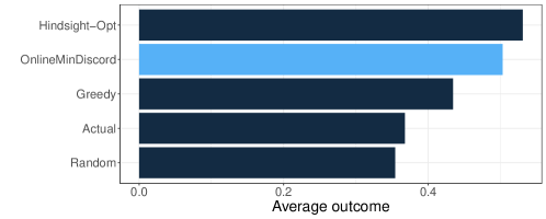
Figure 1: Results of online algorithms on employment for US refugees in 2016.

Figure 1 shows the results. OnlineMinDiscord achieves 95% of the employment score of the hindsight-optimal solution. This is compared to the greedy, random, and “actual assignment” benchmarks, which achieve 81%, 67%, and 69% of the hindsight optimal employment levels, respectively. We note that the 5% optimality gap of OnlineMinDiscord is primarily due to nonstationarity in the arrival process. When the arrival dates of the cases are randomly perturbed—mimicking a stationary process—the optimality percentage of the proposed algorithm increases to 99.5%. This was calculated as the average optimality percentage across five random instances, where in each instance the arrival dates of the cases are randomly shuffled; in each of these instances, the optimality percentage was between 99.4% and 99.6%. However, the focus of this paper is on the performance of the proposed algorithms on the real, non-stationary, arrival data.

4.3 Allocation Imbalance Under Outcome Maximization

Although the proposed method performs well in terms of maximizing outcomes, it results in significant wait time and idle time at the localities. To demonstrate the periodic imbalance resulting from applying OnlineMinDiscord, Figure 2 (left) shows the cumulative allocation to the largest nine locations over the horizon. Figure 2 (right) shows the build-up at each location over time, computed according to Equation (2). Waiting time can be calculated as the area under the curves in Figure 2 (right), and idle time occurs when these curves are at a value zero. Under OnlineMinDiscord, there is severe imbalance that manifests at almost all locations. Assuming (without loss of generality) one arrival per period, and thus a horizon of 1,175 periods, the average number of idle periods per location is 212 periods. Additionally, when a location is not idle, the average wait time per period per location is 15.4 cases. Thus, each location is idle about 18% of the time, and when they are not idle, has a backlog of over fifteen cases on average.

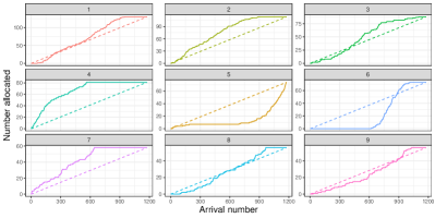
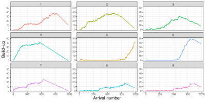
Figure 2: Allocation to top 9 locations over time (left), and build-up at each location (right) using Algorithm OnlineMinDiscord.

We note that this is not simply a consequence of the particular choice of online algorithm, nor entirely a consequence of the online nature of the problem: even the hindsight-optimal solution results in imbalance over time. A figure demonstrating the imbalance resulting from the hindsight-optimal solution can be found in Appendix 12.

So what accounts for this periodic imbalance over time? Consider the non-stationarity of arrivals. If a batch of “similar” cases arrives, imbalance will likely occur. The goal of OnlineMinDiscord is strictly to maximize outcomes while meeting the capacity constraints at the end of the horizon, not to ensure balance over time, and thus a batch of cases may all be assigned to the same location. In reality, because refugee inflows are, in part, due to international events, there can be clustering of arrivals with specific background characteristics—particularly with respect to country of origin, which is one of the predictors that underlies the employment scores. Thus, it can be common for batches of “similar” cases to arrive close together, contributing to an imbalanced allocation. These observations motivate the use of an algorithm that actively balances the allocation over time to each locality. The proposed method is described in the next section.

Further, even if the arrival process were truly stationary, explicitly balancing the allocation may still be desirable to mitigate against random deviations from a balanced allocation. Appendix 12 shows the allocation over time and build-up for five random instances where the arrival dates of the cases are randomly permuted in order to mimic a stationary process.

5 Allocation Balancing

In this section, the additional objective of minimizing wait time and idle time is added to the online matching problem. Because the number of slots at each location is fixed, minimizing wait time is effectively equivalent to minimizing wait time and idle time. Therefore, we focus on minimizing wait time explicitly, while also noting the subsequent impact of the proposed methods on idle time. For simplicity of exposition, we will assume that the cost of wait time is identical across locations, although extending the algorithm to the non-identical case is straightforward.

5.1 Offline Benchmark

First, consider a new variant of the offline benchmark. The new offline allocation-balancing outcome-maximizing optimization problem is given by:

$$\operatorname*{max}_{\mathbf{Z},\mathbf{b}} \sum_{t=1}^{T}\sum_{j=1}^{M}w_{tj}z_{tj}-\gamma\sum_{t=1}^{T}\sum_{j=1}^{M}\lceil b_{j}(t)-1\rceil\mathbbm{1}\{b_{j}(t)>1\}$$ (Balance)

s.t. $$\sum_{j=1}^{M}z_{tj}=1\;\;\;\forall\;\;\;t\in[T]$$

$$\sum_{t=1}^{T}z_{tj}=s_{j}\;\;\;\forall\;\;\;j\in[M]$$

$$b_{j}(t)=\max\{0,b_{j}(t-1)+z_{tj}-\rho_{j}\}\;\;\;\forall\;\;\;t\in\{2,...,T\},\;j\in[M]$$

$$b_{j}(1)=z_{1j}\;\;\;\forall\;\;\;j\in[M]$$

$$\mathbf{Z}\in\{0,1\}^{T\times M}$$

Recall that $b_{j}(t)$ denotes the build-up at location $j$ at time $t$, and $\rho_{j}$ is again the processing rate of location $j$. In the objective function of Balance, wait time cost is incurred when $b_{j}(t)>1$, and $\lceil b_{j}(t)-1\rceil$ is the number of cases waiting at time $t$. The parameter $\gamma$ is a weight that balances the trade-off between outcomes and wait time cost, and can be thought of as the cost of wait time. In practice, this parameter could be set either according to a cost-benefit analysis such that the units of measure were commensurate with one another, or according to an empirically driven decision on a value that results in acceptable balance across locations over time.

Let Balance$(\mathbf{W}_{t},\tilde{\mathbf{s}}(t-1),\mathbf{b}(t-1))$ denote solving Balance from time $t$ onward, for population $\mathbf{W}_{t}$ with slots $\tilde{\mathbf{s}}(t-1)$ and initial buildup $\mathbf{b}(t-1)$. Recall that in OnlineMinDiscord, OutcomeMax is solved $K$ times for each new arrival, each time using a randomly generated sample of future arrivals. This same approach will be used to develop the new online allocation-balancing outcome-maximizing assignment algorithm.

Consider the most straightforward extension of OnlineMinDiscord. For $K$ randomly drawn populations $\{\mathbf{W}_{t+1}^{k}\}_{k=1,...,K}$, we would solve Problem Balance$([\mathbf{w}_{t};\mathbf{W}^{k}_{t+1}],\tilde{\mathbf{s}}(t-1),\mathbf{b}(t-1))$. The final choice of location for case $t$ would again be given by

$$\operatorname*{arg\,max}_{j\in[M]}\sum_{k\in[K]}z^{k}_{tj},$$

where $\mathbf{Z}^{k}$ is the optimal assignment matrix for the $k$th random draw.

Unfortunately, unlike OutcomeMax, Balance cannot be solved to optimality as a linear program. The variables $b_{j}(t)$ are defined by non-linear expressions, and the objective function of Balance is also non-linear. Due to advances in mixed-integer programming (MIP), Balance can still be solved using state-of-the-art MIP solvers. However, solving this problem $K$ times may take minutes or even hours, depending on the length of the horizon. For this reason, we propose an alternative method that uses an approximate version of Balance in the online algorithm that results in the same run-time as OnlineMinDiscord.

5.2 Online Allocation Balancing Algorithm

In this section we propose an approximate version of Balance to use as the offline benchmark in the online allocation-balancing algorithm. Balance is difficult to solve because wait time and idle time depend on the entire sequence of arrivals and are non-linear functions of the assignment variables. In the online setting, the past assignments to each location are readily observable. Thus, at time $t$, the online algorithm has access to $b_{j}(t-1)$ for all locations $j$. We take advantage of this information when constructing the approximation method.

Consider the following problem at time $t$:

$$\operatorname*{max}_{\mathbf{Z}} \sum_{l=t}^{T}\sum_{j=1}^{M}w_{lj}z_{lj}-\gamma\sum_{j=1}^{M}z_{tj}\left\lceil\frac{b_{j}(t-1)-\rho_{j}}{\rho_{j}}\right\rceil\mathbbm{1}\{b_{j}(t-1)>0\}$$ (GBalance)

s.t. $$\sum_{j=1}^{M}z_{lj}=1\;\;\;\;\;\;\forall\;\;\;l\in\{t,...,T\}$$

$$\sum_{l=t}^{T}z_{lj}=\tilde{s}_{j}(t)\;\;\;\forall\;\;\;j\in[M]$$

$$\mathbf{Z}\in\{0,1\}^{N\times M}$$

Notice that GBalance takes $\mathbf{b}(t-1)$ as input, and only weights the employment score of case $t$ by the marginal wait time cost incurred by case $t$. The wait time that case $t$ experiences if assigned to location $j$ is the amount of time until all earlier cases are done being processed, starting from time $t$, namely $\left\lceil\frac{b_{j}(t-1)-\rho_{j}}{\rho_{j}}\right\rceil$. Because $\mathbf{b}(t-1)$ is known prior to the $t$-th arrival, GBalance has a linear objective function. Thus, the optimal solution to GBalance can be found by solving its LP relaxation. In fact, solving GBalance is as fast as solving OutcomeMax, making this problem appealing for use in an online setting.

To build intuition for GBalance, we present the following lemma, which bridges Balance and GBalance.

Lemma 5.1

The objective function of Balance is equivalent to

$$\sum_{t=1}^{T}\sum_{j=1}^{M}w_{tj}z_{tj}-\gamma\sum_{t=1}^{T}\sum_{j=1}^{M}z_{tj}\left\lceil\frac{b_{j}(t-1)-\rho_{j}}{\rho_{j}}\right\rceil\mathbbm{1}\{b_{j}(t-1)>0\}.$$ (6)

The objective function of GBalance is a greedy version of Expression 6—namely, it does not calculate wait time for the entire horizon, but does so only for the current arrival. Therefore, it handles wait time in a greedy fashion (hence the name Greedy Balance).

Although the greedy method does not work well when it comes to outcome maximization, it does work well for minimizing wait time. The reason that a greedy approach does not work well for outcome maximization is that taking a slot from location $j$—especially if this location is “good” for many cases—is irreversible and has implications on the achievable outcomes for future arrivals. In terms of wait time, taking a slot from location $j$ has two effects. First, this action immediately increases the build-up at location $j$. This could make it less likely for arrivals in the near-future to be assigned to location $j$, which could be consequential especially if, for some of these arrivals, location $j$ is highly desirable. However, this effect is short-lived: it is only relevant if an arrival in the near future (i.e., before the current arrival can be fully processed) would also be sent to location $j$. Thus, if there are many locations, or if location $j$ has few slots, this immediate effect is mitigated.

Sending case $t$ to location $j$ also has an indirect effect on the overall congestion of the system. Taking a slot at location $j$ means that location $j$ will be less congested in the future. Specifically, at each location, the ratio of remaining slots to the remaining time horizon impacts the expected wait time across all sample paths. However, for a given sample path, the arrival order is more consequential for wait time than a small change in the capacity vector. Therefore, especially when the horizon is long, this effect is likely to be limited. Additionally, to the extent that current build-up is a proxy for future build-up, the greedy approach already takes congestion into account.

Accordingly, we propose a new method for assigning a single arrival to a location. Method 2 is similar to Method 1, but assigns the current arrival based on the solution to GBalance instead of OutcomeMax as in Method 1.

Method 2 (Allocation-Balancing MinDiscord)

blank
Case $t$ is assigned to location

$$\phi(t)=\operatorname*{arg\,max}_{j\in[M]}\sum_{k\in[K]}z^{k}_{tj},$$

where

$$\mathbf{Z}^{k}=\operatorname*{arg\,max}_{\mathbf{Z}} \text{\ref{prob:offline_balance_greedy}}\left([\mathbf{w}_{t};\mathbf{W}^{k}_{t+1}],\tilde{\mathbf{s}}(t-1),\mathbf{b}(t-1)\right)$$

The new online algorithm, based on Method 2, is presented below in Algorithm OnlineBalance.

Algorithm OnlineBalance (Allocation-Balancing Online Assignment)

1:initialize $\tilde{s}_{j}(0)\leftarrow s_{j}$ for all $j\in\{1,...,M\}$

2:for $t$ in $1,...,T$ do

3:     for $k$ in $1,...,K$ do

4:         $\mathbf{W}_{t+1}^{k}\leftarrow$ $T-t$ randomly drawn cases from set $\mathcal{A}$

5:         $\mathbf{Z}^{k}\leftarrow\operatorname*{arg\,min}$ GBalance$([\mathbf{w}_{t};\mathbf{W}^{k}_{t+1}],\tilde{\mathbf{s}}(t-1),\mathbf{b}(t-1))$

6:     end for

7:     $\phi(t)\leftarrow\operatorname*{arg\,max}_{j}\sum_{k}z^{k}_{tj}$

8:     $\tilde{\mathbf{s}}(t)\leftarrow\tilde{\mathbf{s}}(t-1)-e_{\phi(t)}$

9:     $\mathbf{b}(t)\leftarrow\max\{0,(\mathbf{b}(t-1)-\boldsymbol{\rho})\mathbbm{1}_{t\geq 2}+e_{\phi(t)}\}$

10:end for

11:return $\Phi^{GB}=\{\phi(t)\}_{t=1...T}$

To emphasize the fact that solving GBalance is equivalent to solving OutcomeMax with modified weights, we note that the inner loop of OnlineBalance can equivalently be written as:

$$\SingleSpacedXI \tilde{w}_{tj}\leftarrow w_{tj}-\gamma\left\lceil\frac{b_{j}(t-1)-\rho_{j}}{\rho_{j}}\right\rceil\mathbbm{1}\{b_{j}(t-1)>0\}\;\;\;\forall\;j\in[M]$$

$$\mathbf{W}_{t+1}^{k}\leftarrow T-t\text{ randomly drawn cases from set }\mathcal{A}$$

$$\mathbf{z}^{k}\leftarrow\operatorname*{arg\,min}\textsc{Offline}([\tilde{\mathbf{w}}_{t};\mathbf{W}_{t+1}^{k}],\tilde{\mathbf{s}}(t-1))$$

5.3 Results and Discussion

Recall that the parameter $\gamma$ controls the trade-off between allocation balancing and outcome maximization. Therefore, the policymaker can choose or tune this parameter to obtain the desired level of employment and allocation balance. In situations in which the payoff/cost of outcomes, wait time, and idle time can all be measured in or converted to a common metric (such as payoff/cost in dollars), policymakers might want to set $\gamma$ to the specific value that leads to maximization of that common metric. Another approach would be to use empirical experiments to tune $\gamma$ to a value that establishes an acceptable degree of balance across locations over time.

Figure 3 shows the employment level and wait time incurred by various values of $\gamma$. Although we do not show idle time, we note that it is strongly correlated with wait time. The vertical axis of Figure 3 shows the employment level under a particular value of $\gamma$ divided by the employment level when $\gamma=0$ (i.e., under pure outcome-maximization). Interestingly, the highest employment level is not achieved when $\gamma=0$, but when $\gamma$ is slightly positive, likely due to the non-stationarity in the arrival process. This result may simply be due to idiosyncrasies in the particular arrival data rather than necessarily a general result. That being said, the results at least tentatively suggest that, aside from the direct load balancing benefits, the allocation-balancing method may also help to amplify the benefits and/or add robustness to the outcome-maximization objective in the face of non-stationarity.

As can be seen from Figure 3, wait time can be dramatically reduced with virtually no loss (and, again, perhaps with a gain) in employment. The ideal region in Figure 3 is the top left—where wait time is minimized, and employment is maximized. Based on this plot, a policymaker could choose an appropriate value of $\gamma$ to achieve their desired balance of employment versus allocation balancing.

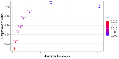
Figure 3: Trade-off between outcome maximization and allocation balancing.

To illustrate these results in greater detail, Figure 4 shows the allocation of the 2016 arrivals using OnlineBalance with $\gamma=0.005$. This can be compared to Figure 1. From visual inspection alone, it is clear that applying OnlineBalance results in a much more balanced allocation over time. Indeed, the average idle time per location in Figure 4 is 51 days (compared to 212 days under OnlineMinDiscord), and the average wait time per non-idle day is 1.87 (compared to 15.4). Furthermore, the total employment score obtained using OnlineBalance with $\gamma=0.005$ is 98% of the score obtained with OnlineMinDiscord.

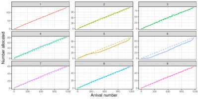
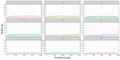
Figure 4: Allocation to top 9 locations over time, using heuristic with $\gamma=.005$.

6 Additional Benefits of Allocation Balancing

This section discusses additional benefits of using OnlineBalance as opposed to OnlineMinDiscord. While OnlineBalance was developed in order to achieve balanced workloads across the localities, allocation balancing also helps to address two other potential issues.

6.1 Unknown $T$

Up until this section, it was assumed that the number of arrivals in a given time horizon, and capacities for each location, are known a priori. Furthermore, it was assumed that $\sum_{j}s_{j}=T$. In the real-world setting of refugee resettlement, the number of refugees (or asylum seekers) arriving in a given time period is typically not known exactly. For instance, in the context of asylum seeker assignment in European countries like Switzerland, authorities can make projections, but the exact number of people who will arrive at their borders and claim asylum each year is fundamentally uncertain. Thus, target quotas can be set for each of the 26 Swiss cantons on the basis of annual arrival projections, but those quotas must be revised throughout the year as the number of actual arrivals becomes clear.

Therefore, in practice the assumption of known $T$ and $\mathbf{s}$—which underlies Algorithms OnlineMinDiscord and OnlineBalance—is often violated. The method proposed by Ahani et al. (2021) is also highly dependent on the assumption of known $T$ and capacities. Ahani et al. (2021) address the issue of unknown $T$ by demonstrating that their proposed methods still perform well (in terms of maximizing outcomes) under capacity revisions, and propose strategies for revising the capacities during the year. A similar dynamic revision method is also currently being used in the Swiss pilot program, which uses the OnlineMinDiscord algorithm.

Note that the initial number of slots allocated to each location is based upon a desired proportionality key across locations (e.g. proportional to the total population or other measures of capacity and resources in the location). Therefore, adding new slots if needed is a straightforward task: they are simply added according to the predetermined proportion. However, adjusting the capacities downward if the number of arrivals is less than expected is more difficult. Refugees that have already been assigned to a location cannot be reassigned. Suppose that at time $t^{\prime}$, it is realized that the total number of arrivals will be less than initially expected. If location $j$’s slots have already been used up by time $t^{\prime}$, no slots can be removed from location $j$. Thus, the final allocation of refugees to locations will end up imbalanced at the end of the year. If, however, the algorithm maintains balance throughout the year, scaling $T$ upward or downward has little impact on performance or balance. By expressly maintaining this balance, OnlineBalance implicitly accommodates uncertainty in $T$ effectively, straightforwardly, and without necessitating additional strategies.

6.2 Exploration

Although this paper does not focus on the outcome prediction methodology, the prediction and assignment steps are not completely independent. In this paper, it was assumed that the outcome weights are known. In practice, these outcome weights are estimated from historical data. To use the proposed methods, reliable weights must be determined for every combination of covariates and locations. If these weights are generated via statistical estimation procedures, maintaining some degree of exploration—assigning similar cases to different locations—is crucial to the resiliency of the estimation performance given the non-stationarity of the environment. The need for exploration in situations where individual decisions are made on the basis of estimated payoffs is, of course, a well-known issue and is not unique to the refugee matching context.

A non-stationary contextual bandit framework could be used to formally address this problem. However, without formalizing the bandit version of this problem, we note that the balancing heuristic achieves higher levels of exploration than a purely outcome-maximizing approach. Intuitively, because of the balancing component of the objective function, the assignment of a case not only depends on their predicted employment score and the remaining capacity vector (as in an outcome-maximizing online algorithm), but also depends on the current build-up at each location.

To demonstrate this idea, we run OnlineMinDiscord and OnlineBalance 100 times each for the last 500 arriving cases in 2016, where the arrival order is randomly permuted in each of the 100 iterations. Let case $i$ be the case that arrived $i-$th in the true arrival sequence. In the 100 random iterations, they could arrive on any of the 500 days. For each case, we compute the number of times that they are assigned to each location. Let $\ell_{i,1}$ be the location that case $i$ is most often assigned to, $\ell_{i,2}$ be their second most assigned location, etc. Let $n_{\ell_{i,k}}$ be the number of times that case $i$ was assigned to their $k$th most-assigned location. Figure 5 shows a bar chart of the average value of $n_{\ell_{i,k}}/100$ under OnlineMinDiscord and OnlineBalance. Note that $\sum_{k}n_{\ell_{i,k}}=100$ for each case $i$. If $n_{\ell_{i,1}}=100$, then $n_{\ell_{i,k}}=0$ for all $k>1$, and case $i$ did not “explore” at all. The more uniform the values of $n_{\ell_{i,k}}$, the greater the exploration.

Based on visual inspection of Figure 5, it is clear that OnlineBalance results in greater exploration than OnlineMinDiscord. Under OnlineBalance, the average value of $n_{\ell_{i,1}}/100$ is less than 0.4, whereas under OnlineMinDiscord the value is about 0.475. Thus, under OnlineBalance, on average a case is assigned to their “top” location less than 40% of the time, whereas under OnlineMinDiscord, they are assigned to their top location almost 50% of the time. Additionally, the average number of unique locations the same case was assigned to under OnlineMinDiscord was 8.17, versus 13.3 under OnlineBalance.

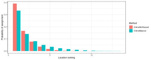
Figure 5: Average probability of being assigned to the $k$th location, where locations are ordered at the case-level according to their assignment probabilities.

7 Conclusions

This study proposed two assignment algorithms for matching refugees to localities. The first method seeks to maximize the employment scores of all refugees over a horizon by minimizing the probability of disagreement between the online algorithm and an offline benchmark. On the US refugee resettlement data used in this study, this method is able to achieve 95% of the hindsight-optimal employment score. This is a significant improvement over the actual historical assignment, random assignment, and greedy assignment, which achieve 69%, 67% and 82% of the hindsight-optimal employment scores, respectively.

However, this algorithm—and any outcome-maximizing algorithm—may result in severe periodic imbalance across the localities. In the setting of refugee resettlement, this imbalance is extremely undesirable as it leads to increased strain and highly variable workloads for the local caseworkers, service providers, and other community members who help each newly arriving family get settled. Therefore, we proposed a second assignment algorithm that directly seeks to balance the allocation over time to the localities, while still achieving high outcome levels. On the US refugee resettlement data used in this study, the allocation balancing method is able to significantly increase balance with little to no loss in employment, depending on the importance placed on allocation balance versus employment scores.

By all indications, the challenges and scale of forced migration will continue to grow into the future. The methods presented here build upon recent research on outcome-based refugee assignment and could be integrated into refugee resettlement and asylum programs in many host countries—such as the United States, Netherlands, Switzerland, Sweden, and Norway—to help improve the lives of some of the world’s most vulnerable populations.

We acknowledge funding from the Rockefeller Foundation, Schmidt Futures, and the Charles Koch Foundation. The funders had no role in the data collection, analysis, decision to publish, or preparation of the manuscript. We thank the Lutheran Immigration and Refugee Service (LIRS) for access to data and guidance. The US refugee data used in this study were provided under a collaboration research agreement with LIRS. This agreement requires that these data not be transferred or disclosed. We also thank the Swiss State Secretariat for Migration (SEM) for guidance and support. Finally, we are grateful to Daniel Freund and Jens Hainmueller for helpful comments.

Appendix

8 Regret of OnlineMinDiscord

The total regret of OnlineMinDiscord is defined as:

$$R(\ref{alg:modal}):=w(\Phi^{MD})-w(\Phi^{*})$$

where $w(\cdot)$ is defined in Equation (1) and $\Phi^{*}$ denotes the hindsight-optimal matching (namely, the solution to OutcomeMax$(\mathbf{W})$ where $\mathbf{W}$ is the true test cohort).

Suppose that, at time $t$, an arbitrary online algorithm assigns case $t$ to location $\phi(t)$. The expected disagreement cost is defined as

$$d_{t}(\phi(t),S_{t})=\mathbb{E}[ \ref{prob:offline}([\mathbf{w}_{t};\mathbf{W}(\omega)_{t+1}],\tilde{\mathbf{s}}(t-1))$$ (7)

$$-(w_{t\phi(t)}+\ref{prob:offline}(\mathbf{W}(\omega)_{t+1},\tilde{\mathbf{s}}(t-1)-e_{\phi(t)}))|S_{t}].$$

This is the amount that the online algorithm loses at time $t$ compared to the offline benchmark starting in the same state. Lemma 8.1 below characterizes the expected regret of OutcomeMax in terms of the disagreement probabilities, analogous to Lemma 1 of Vera and Banerjee [2020].

Lemma 8.1

Let $\phi(t)^{MD}$ be the location that case $t$ is assigned to under OnlineMinDiscord. Under the stage-wise independence and stationarity assumptions,

$$\mathbb{E}[R(\ref{alg:modal})]=\sum_{t=1}^{T}d_{t}(\phi(t)^{MD},S_{t})\leq\delta_{max}\sum_{t=1}^{T}q(\phi(t)^{MD},S_{t}),$$

where $\delta_{max}$ is an upper bound on the disagreement cost.

Before proving Lemma 5.1, note that in the setting of this paper, the outcome scores are probabilities so the disagreement costs cannot be greater than one. Thus, an upper bound on the expected regret is simply given by $\sum_{t=1}^{T}q(\phi(t)^{MD},S_{t})$. As mentioned before, note that OnlineMinDiscord does not minimize the expected disagreement cost at each step, but rather it minimizes the probability of disagreement at each step. Therefore, it minimizes an upper bound on the expected regret (Lemma 8.1). Appendix 13.1 presents an alternative version of the algorithm that does minimize the expected disagreement cost at each step.

Proof 8.2

Proof of Lemma 8.1 Let $v(\cdot)$ denote the objective value of a particular optimization problem. Let $\mathbf{W}$ denote the employment scores for a cohort of interest. Let $\Psi_{t}^{*}(\tilde{\mathbf{s}}(t-1)):=\mathbb{E}_{\mathbf{W}_{t}}[v(\ref{prob:offline}(\mathbf{W}_{t},\tilde{\mathbf{s}}(t-1)))]$ denote the expected sum of outcome scores of the optimal assignment for all cases $t$ onward, starting with capacity vector $\tilde{\mathbf{s}}(t-1)$.

Given the assignment of case $t$ to $\phi(t)$, the expected disagreement cost at time $t$ can be written as:

$$d_{t}=\mathbb{E}_{\mathbf{W}_{t+1}}[\Psi^{*}_{t}(\tilde{\mathbf{s}}(t-1))-\left(w_{t\phi(t)}+\Psi_{t+1}^{*}(\tilde{\mathbf{s}}(t-1)-e_{\phi(t)})\right)|\mathbf{w}_{t}].$$

This is equivalent to Expression 7 in the main text, where we have dropped the arguments in $d_{t}(\cdot)$ for simplicity.

Note that the expression above relies on the stage-wise independence assumption. Rearranged, and showing the same result for case $t+1$, yields:

$$w_{t\phi(t)}=\mathbb{E}_{\mathbf{W}_{t+1}}[\Psi_{t}^{*}(\tilde{\mathbf{s}}(t-1))|\mathbf{w}_{t}]-\mathbb{E}_{\mathbf{W}_{t+1}}[\Psi_{t+1}^{*}(\tilde{\mathbf{s}}(t-1)-e_{\phi(t)})|\mathbf{w}_{t}]+d_{t}$$

$$w_{(t+1)\phi(t+1)}=\mathbb{E}_{\mathbf{W}_{t+2}}[\Psi_{t+1}^{*}(\tilde{\mathbf{s}}(t))|\mathbf{w}_{t+1}]-\mathbb{E}_{\mathbf{W}_{t+2}}[\Psi_{t+2}^{*}(\tilde{\mathbf{s}}(t)-e_{\phi(t+1)})|\mathbf{w}_{t+1}]+d_{t+1}$$

Now note that, by the assumptions of stationarity and stagewise independence:

$$\mathbb{E}_{\mathbf{W}_{t+1}}[\Psi_{t+1}^{*}(\tilde{\mathbf{s}}(t-1)-e_{\phi(t)})|\mathbf{w}_{t}]=\mathbb{E}_{\mathbf{W}_{t+1}}[\mathbb{E}_{\mathbf{W}_{t+2}}[\Psi_{t+1}^{*}(\tilde{\mathbf{s}}(t))|\mathbf{w}_{t+1},\mathbf{w}_{t}]].$$

where $\tilde{\mathbf{s}}(t)=\tilde{\mathbf{s}}(t-1)-e_{\phi(t)}$.

Therefore, the expected sum of the outcome scores for assigning each item via $\Phi$ can be written as:

$$E_{\mathbf{W}}\left[\sum_{t=1}^{T}w_{t\phi(t)}\right]=E_{\mathbf{W}}\left[\Psi^{*}_{1}(\mathbf{s})\right]+\sum_{t=1}^{T}d_{t},$$

and thus the expected regret of assignment $\Phi$ is given by

$$\mathbb{E}[R(\phi)]=\mathbb{E}_{\mathbf{W}}\left[\sum_{t=1}^{T}w_{t\phi(t)}-\Psi^{*}_{1}(\mathbf{s})\right]=\sum_{t=1}^{T}d_{t}.$$

This states that the expected regret of an assignment $\Phi$ is equal to the sum of the expected disagreement costs at each time step. Note that this expression for regret applies to any online algorithm $\Phi$.

Therefore, it is natural to develop an online assignment algorithm that minimizes the disagreement cost at each time period. The algorithm OnlineMinDiscord does not minimize the disagreement cost explicitly, but instead minimizes the probability of disagreement. Appendix 13.1 proposes an online algorithm that minimizes the disagreement cost directly. This algorithm is more computationally taxing than OnlineMinDiscord.

The sum of expected disagreement costs can also be written as

$$\mathbb{E}\left[\sum_{t=1}^{T}d_{t}\mathbbm{1}\{Q(\phi(t),S_{t})\}\right].$$

where $Q(\phi(t),S_{t})$ is the event that assignment $\phi(t)$ disagrees with the offline benchmark at time $t$. If there is no disagreement, then the disagreement cost is zero. This expression can be upper bounded by:

$$\mathbb{E}\left[\sum_{t=1}^{T}d_{t}\mathbbm{1}\{Q(\phi(t),S_{t})\}\right]\leq\delta_{max}\mathbb{E}\left[\sum_{t=1}^{T}\mathbbm{1}\{Q(\phi(t),S_{t})\}\right]=\delta_{max}\sum_{t=1}^{T}q(\phi(t),S_{t})$$

where $\delta_{max}$ is an upper bound on the disagreement costs. In our setting, because the outcome scores correspond to employment probabilities, the disagreement cost in any time period is upper bounded by one. Thus, the expected total regret can be bounded above by the number of disagreements:

$$\mathbb{E}[R(\phi)]\leq\mathbb{E}\left[\sum_{t=1}^{T}\mathbbm{1}\{Q(\phi(t),S_{t})\}\right]=\sum_{t=1}^{T}q(\phi(t),S_{t}).$$

where $q(\phi(t),S_{t})$ is again the disagreement probability of action $\phi(t)$ in state $S_{t}$. $\square$

9 Proof of Lemma 5.1

Recall that $b_{j}(t)=b_{j}(t-1)-\rho_{j}+z_{tj}$ is the buildup after the assignment at time $t$ but before the processing at time $t$, and $b_{j}(1)=z_{1j}$. In order to prove the lemma, we must show that the following expressions are equivalent:

$$\sum_{t=1}^{T}\sum_{j=1}^{M}\lceil b_{j}(t)-1\rceil\mathbbm{1}\{b_{j}(t)>1\},$$ (8)

and

$$\sum_{t=1}^{T}\sum_{j=1}^{M}z_{tj}\left\lceil\frac{b_{j}(t-1)-\rho_{j}}{\rho_{j}}\right\rceil\mathbbm{1}\{b_{j}(t-1)>0\}$$ (9)

The first expression is the wait time component of the objective of Balance. Intuitively, the former expression calculates the wait time cost incurred per period, whereas the latter calculates the costs per case. To see this, notice that $\lceil b_{j}(t)-1\rceil$ is the number of cases waiting at time $t$, and $\left\lceil\frac{b_{j}(t-1)-\rho_{j}}{\rho_{j}}\right\rceil$ is the number of periods that case $t$ waits before being serviced. Let $q_{tj}:=\left\lceil\frac{b_{j}(t-1)-\rho_{j}}{\rho_{j}}\right\rceil$.

Now consider the following string of equalities for expression 9:

$$\sum_{c=1}^{T}z_{cj}q_{cj}= \sum_{c=1}^{T}z_{cj}\sum_{t=c}^{c+q_{cj}-1}1$$

$$= \sum_{c=1}^{T}\sum_{t=1}^{T}z_{cj}\mathbbm{1}\{t\in\{c,...,c+q_{cj}-1\}\}$$

$$= \sum_{t=1}^{T}\sum_{c=1}^{T}z_{cj}\mathbbm{1}\{t\in\{c,...,c+q_{cj}-1\}\}.$$

Intuitively, the last equality above exactly counts the number of cases that are waiting to be processed at time $t$. Case $c$ is waiting in time periods $t\in\{c,...,c+q_{cj}-1\}$ and is being processed in time periods $t\in\{c+q_{cj},c+\left\lceil\frac{b_{j}(t-1)-\rho_{j}+1}{\rho_{j}}\right\rceil-1\}$ (since $\lceil 1/\rho_{j}\rceil$ is the processing time). Therefore, $\lceil b_{j}(t)\rceil$—which is the number of cases being processed or serviced at time $t$, is equal to $\sum_{c=1}^{T}z_{cj}\mathbbm{1}\{t\in\{c,...,c+q_{cj}-1\}\}$.

Thus, we can write

$$\sum_{c=1}^{T}z_{cj}\mathbbm{1}\left\{t\in\left\{c,...,c+q_{cj}-1\right\}\right\}$$

$$=\lceil b_{j}(t)\rceil-\sum_{c=1}^{T}z_{cj}\mathbbm{1}\left\{t\in\left\{c+q_{cj},...,c+\left\lceil\frac{b_{j}(t-1)-\rho_{j}+1}{\rho_{j}}\right\rceil-1\right\}\right\}.$$

Since only one case can be processed at a time, the term

$$\sum_{c=1}^{T}z_{cj}\mathbbm{1}\left\{t\in\left\{c+q_{cj},...,c+\left\lceil\frac{b_{j}(c-1)-\rho_{j}+1}{\rho_{j}}\right\rceil-1\right\}\right\}$$

can be at most equal to one for each $t$, and is exactly equal to one unless location $j$ is idle at time $t$. Otherwise, this term is zero. Therefore,

$$\sum_{c=1}^{T}z_{cj}\mathbbm{1}\left\{t\in\left\{c+q_{cj},...,c+\left\lceil\frac{b_{j}(c-1)-\rho_{j}+1}{\rho_{j}}\right\rceil-1\right\}\right\}=\mathbbm{1}\{b_{j}(t)>0\},$$

and thus

$$\sum_{c=1}^{T}z_{cj}\mathbbm{1}\left\{t\in\left\{c,...,c+q_{cj}-1\right\}\right\}=\lceil b_{j}(t)\rceil-\mathbbm{1}\{b_{j}(t)>0\}=\lceil b_{j}(t)-1\rceil\mathbbm{1}\{b_{j}(t)>1\}.$$

Therefore, the objective function of Problem Balance can be re-written as

$$\sum_{t=1}^{T}\sum_{j=1}^{M}w_{tj}z_{tj}-\gamma\sum_{t=1}^{T}\sum_{j=1}^{M}z_{tj}\left\lceil\frac{b_{j}(t-1)-\rho_{j}}{\rho_{j}}\right\rceil\mathbbm{1}\{b_{j}(t-1)>0\}.$$

$\square$

10 Data scope

As noted in the main text, we included only free cases in the empirical demonstrations of our methods, and the location quotas that were employed were based on the actual distribution of free cases in the time frame of interest. We excluded cases with existing family ties from these demonstrations because they must be assigned to wherever their family is, regardless of any other considerations. Hence, given their predetermined location assignments, it is not possible to optimize their placement to improve outcomes or to balance their allocation. That being said, their exclusion from our empirical demonstrations does constitute a deviation from a real-world implementation, though the degree of deviation depends on the extent to which family-tie cases "compete" for location slots with free cases and the amount of impact they have on location build-up.

With respect to the former consideration, at one extreme is a situation in which there is no advance information on how many arrivals will have family ties (and where those family ties will be), such that assignment of both free cases and family-tie cases must be made according to a shared capacity system, where they are "competing" for the same slots. At the other extreme, family-tie arrivals can be known, determined, or selected in advance. This would allow the location capacities to be separated out for free cases (i.e. the total quotas net of those dedicated to the family-tie cases), as in how the empirical demonstrations have been presented in this paper. In the United States and other countries, the reality will be somewhere in between these two extremes, as it is generally possible to use recent trends and knowledge of prior arrivals who have indicated they have "trailing" family members to control or project (with a degree of uncertainty) the number of arrivals who will have family ties and where those ties are.

With respect to the latter consideration on the contribution of the family-tie cases to location build-up, it is again useful to consider two extremes. At one extreme, those cases would contribute to build-up in the exact same manner as free cases, which would then have implications for balancing the dynamic assignment decisions made for free cases. At the other extreme, the family networks and relationships that family-tie cases have at their receiving locations would eliminate the processing time and costs imposed on resettlement resources and hence result in negligible or no impact on build-up. Again, the reality is somewhere in the middle.

The assignment of family-tie cases could be directly incorporated or subsumed into the algorithms presented in this study in a number of different ways. (The most straightforward way would be to change nothing and simply include the family tie cases while forcing their assignment to their predetermined locations, assuming that quotas are shared and all cases contribute to build-up in the same manner.) The best manner in which to do so and the degree to which it would impact the results for free cases, however, will depend on precisely where on each of the two spectrums described above the reality lies, which would be specific to the implementing institutional context and require detailed guidance from resettlement authorities.

We note that free cases may also have certain location incompatibilities. For example, if a case has certain medical or educational needs, this may prevent them from being assigned to particular localities. These incompatibilities can be included in the proposed algorithms by setting $w_{tj}=-M$, for some large constant $M$, if case $t$ cannot be assigned to location $j$.

11 Scalability of OnlineMinDiscord

Although OutcomeMax can be efficiently solved as an LP, the inner loop of OnlineMinDiscord—namely, solving $K$ iterations of OutcomeMax—could still be time intensive when the horizon is large. For reference, solving OutcomeMax with a horizon of length 500 takes about 0.5 seconds. (This run-time was obtained using Gurobi on a Macbook Pro with a 2.3 GHz Dual-Core Intel Core i5 processor and 8GB of RAM.) Thus, for example, running 10 random trajectories for a horizon of length 3,000 could take about 30 seconds, which is not insignificant. It is not atypical for the largest resettlement agencies in the US to receive over 5,000 cases in a given year. Although runtime is not a first-order concern, it is nonetheless desirable for our algorithms to provide location assignments in a matter of seconds, not minutes.

Thus, we also propose a method to efficiently scale up OnlineMinDiscord when $T$ is large. Instead of simulating the entire remaining horizon of $T-t$ arrivals, the proposed scaling method only samples a portion of the remaining horizon. This method, described next, is independent of OutcomeMax and can be applied to any extant online assignment algorithm.

First, we set a horizon limit, $h$. Instead of drawing $T-t$ units each time step, we draw $\min\{h,T-t\}$ units. Additionally, we replace $\tilde{s}_{j}$ with $\hat{s}_{j}(t)$ in OutcomeMax, where $\hat{s}_{j}(t)$ is a scaled version of the locations’ capacities such that $\sum_{j}\hat{s}_{j}=\min\{h,T-t\}+1$.

The capacities $\hat{s}_{j}(t)$ are determined through the following procedure. For a vector of integers $x$, let expand($x$) be a set consisting of integer elements 1 through length($x$) such that element $i$ is repeated $x_{i}$ times. For example, expand($[2,3,1]$)=$\{1,1,2,2,2,3\}$. The scaled capacity vector $\hat{s}_{j}(t)$ is obtained by randomly sampling $\min\{h,T-t\}+1$ slots, without replacement, from $\texttt{expand}(\tilde{\mathbf{s}}(t))$ and re-grouping these slots based on location. Let the function $\texttt{sample}(x,n)$ denote sampling $n$ elements from the set $x$ without replacement. Then, $\hat{s}_{j}(t)=\sum_{k=1}^{\min\{h,T-t\}}\mathbbm{1}\left\{\texttt{sample}(\texttt{expand}(\tilde{\mathbf{s}}(t)),\min\{h,T-t\})_{k}=j\right\}$. When this scaling method is applied with horizon $h$, OnlineMinDiscord will be denoted by OnlineMinDiscord-H$(h)$.

Another method to reduce run-time, when desirable, is to decrease the number of sampled trajectories in each time step. This method does not improve scalability (i.e., the run-time in each time period still increases super-linearly as a function of the horizon length), however it can decrease run-time by many factors. Figure 6 (left) shows the performance of OnlineMinDiscord using the scaling method with horizons of 50 and 100. Figure 6 (right) shows the performance of OnlineMinDiscord with a smaller number of sample trajectories ($K=1,5$).

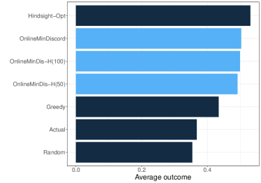
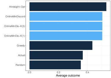
Figure 6: Performance of OnlineMD as the parameters $H$ and $K$ vary.

12 Additional Computations

Figure 7 shows the allocation over time and build-up for five random instances where the test cohort of arrivals (N=1,175) are randomly drawn from the entire population of 2015 and 2016 arrivals, and their arrival order is randomly permuted. In this case, the data generating process is stationary by design, and the population used for sampling is identical, in probability, to the test cohort. Although Figure 7 is much more balanced than Figure 2, random deviations from a balanced allocation can still occur. Thus, even in this case, explicitly enforcing balance is still beneficial. Furthermore, we will show that our balancing method can be implemented with no additional computational costs, and with very little loss in predicted employment.

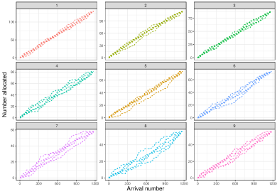
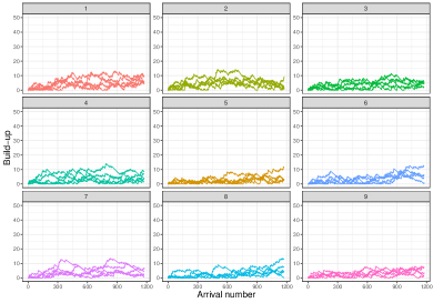
Figure 7: Allocation to top 9 locations over time (left), and build-up at each location (right), with a random arrival order. Results for five random instances are shown.

Figure 8 (left) compares the average employment level achieved by the algorithms proposed in this paper to the potentials algorithm of Ahani et al. [2021]. Figure 8 (right) shows the imbalance resulting from the potentials method of Ahani et al. [2021], which is extremely similar to the imbalance resulting from OnlineMinDiscord.

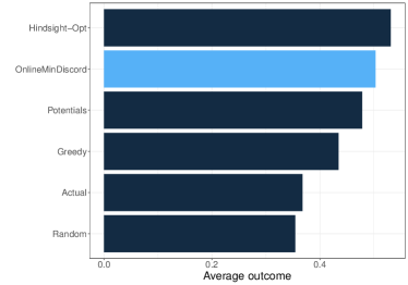
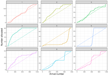
Figure 8: Performance of all outcome-maximizing algorithms, including the “potentials” method introduced by Ahani et al. [2021] (left), and the allocation over time obtained under the potentials method (right).

Figure 9 shows the allocation to the top nine locations over time resulting from the hindsight-optimal solution. Although the imbalance is not as severe as it is under OnlineMinDiscord, significant imbalance still persists. This further motivates the need to develop an algorithm that explicitly takes balance into account.

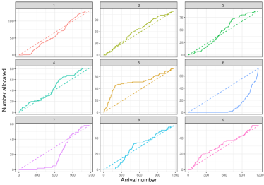
Figure 9: Imbalance of the hindsight-optimal solution for the employment-maximizing assignment problem.

13 Extensions

13.1 Minimum-Risk Formulation

OnlineMinDiscord seeks to minimize the disagreement probability at each time step. An alternative algorithm could instead attempt to directly minimize the expected disagreement cost, which is again given by:

$$d_{t}=\mathbb{E}_{\mathbf{W}_{t+1}}[\Psi^{*}_{t}(\tilde{\mathbf{s}}(t-1))-\left(w_{t\phi(t)}+\Psi_{t+1}^{*}(\tilde{\mathbf{s}}(t-1)-e_{\phi(t)})\right)|\mathbf{w}_{t}]$$

where $\Psi_{t}^{*}(\tilde{\mathbf{s}}):=\mathbb{E}_{\mathbf{W}_{t}}[v(\ref{prob:offline}(\mathbf{W}_{t},\tilde{\mathbf{s}}))]$ denotes the expected sum of employment scores of the optimal assignment for all cases $t$ onward, starting with capacity vector $\tilde{\mathbf{s}}$.

Algorithms such as the potentials method proposed by Ahani et al. [2021] attempt to minimize the disagreement cost by using the dual variables from the capacity constraints of Problem OutcomeMax as approximations of the following quantity for each location $j$:

$$\Psi^{*}_{t}(\tilde{\mathbf{s}}(t-1))-\Psi_{t+1}^{*}(\tilde{\mathbf{s}}(t-1)-j)$$

This approach (as demonstrated in Figure 8) appears to perform quite similarly, if not slightly worse, than OnlineMinDiscord on the data in this study.

The following steps provide a more exact and direct approach to minimizing the disagreement cost in each time step. We refer to this as the “minimum-risk" approach.
For each location $j\in[M]$:

1. Sample $K$ arrival trajectories for cases $t+1$ through $T$, denoted by $\mathbf{W}^{k}_{t+1}$, and compute $d_{tj}^{k}:=\Psi^{*}_{t}(\mathbf{W}^{k}_{t+1},\tilde{\mathbf{s}}(t-1))-\left(w_{tj}+\Psi_{t+1}^{*}(\mathbf{W}^{k}_{t+1},\tilde{\mathbf{s}}(t-1)-j)\right)$ for each trajectory and each $j\in[M]$.

2. Assign case $t$ to $\operatorname*{arg\,min}_{j}\frac{\sum_{k=1}^{K}d_{tj}^{k}}{K}$.

Although this method approximates minimizing the disagreement cost exactly, it requires solving $2\cdot K\cdot M$ instances of OutcomeMax in each time step. If run-time is not an issue, or if both the number of locations and horizon length are average in size, this method would be an appropriate choice over OnlineMinDiscord.

13.2 Batching

In the dynamic formulation of the assignment problem presented above, each item is observed and must be assigned one by one. At the opposite end of the spectrum is, of course, the classic static formulation of the assignment problem, where all items are observed and assigned simultaneously. There also exists a middle ground between the dynamic and static formulations, whereby items are observed and must be assigned in groups or batches. For instance, in the refugee assignment realm, there may be periodic (e.g. weekly, monthly) cohorts of refugee arrivals that can be assigned in batches rather than on a purely one-by-one basis. This section extends the dynamic assignment mechanisms presented above to a batching context.

First, we note that batching cannot hurt the performance of an online algorithm, since the batches can simply be ignored and the units within batches could be assigned one-by-one using the proposed online assignment algorithms. Batching, therefore, only presents an opportunity for improved efficiency. We propose two methods for applying our proposed algorithms to a batched setting.

The first method assigns each case in the batch simultaneously, resulting in the largest efficiency gains. However, it requires solving a MIP many times for each batch. Let $B_{t}$ be the size of the batch arriving at time $t$. For this batch, consider solving the following offline problem, adapted from GBalance.

$$\operatorname*{max}_{\mathbf{Z},\mathbf{b}} \sum_{l=t}^{T}\sum_{j=1}^{M}w_{lj}z_{lj}-\gamma\sum_{l=t}^{t+B_{t}}\sum_{j=1}^{M}z_{lj}\left\lceil\frac{b_{j}(l-1)-\rho_{j}}{\rho_{j}}\right\rceil\mathbbm{1}\{b_{j}(l-1)>0\}$$ (BatchBalance)

s.t. $$\sum_{j}z_{lj}=1\;\;\;\forall\;\;\;l\in\{t,...,t+B_{t}\}$$

$$\sum_{l}z_{lj}=s(t)_{j}\;\;\;\forall\;\;\;j\in[M]$$

$$b_{j}(l)=(b_{j}(l-1)+z_{lj}-\rho_{j})^{+}\;\;\;\forall\;\;\;l\in\{t,...,t+B_{t}\}$$

$$\mathbf{Z}\in\{0,1\}^{N\times M}$$

BatchBalance is equivalent to GBalance except that the objective function includes the wait time and idle time incurred by each case in the current batch. In solving BatchBalance at time $t$, the employment scores $\mathbf{w}_{l}$ are known for $l\in\{t,...,t+B_{t}\}$, but are not known for cases that arrive after time $t+B_{t}$. Thus, following Method 2, we sample $K$ random trajectories of arrivals from time $t+B_{t}+1$ onward is a random trajectory of arrivals from time $t+1+B_{t}$ through $T$. After solving BatchBalance for $K$ random trajectories, the current batch is assigned according to

$$\{\mathbf{z}^{*}_{l}\}_{l\in\{t,...,t+B_{t}\}}=\text{mode}\left(\{\mathbf{z}_{l}^{1}\}_{l\in\{t,...,t+B_{t}\}},...,\{\mathbf{z}_{l}^{K}\}_{l\in\{t,...,t+B_{t}\}}\right)$$

In the pure online setting without batching, this reduces to Method 2. In the pure online setting, each vector $\mathbf{z}_{t}^{k}$ is effectively one dimensional (since it only contains one positive element, it can be mapped to the one-dimensional domain $\{1,...,M\}$). Therefore, the disagreement probabilities could be estimated with a reasonable number of samples. However, with batching, the assignment decision is comprised of $B_{t}$ assignment vectors, and thus can be mapped to a $B_{t}$-dimensional domain ($\{1,...,M\}^{B_{t}}$). Thus, given the combinatorial complexity of the assignment decision with batching, obtaining reasonable estimates of the disagreement probabilities potentially requires many more sample trajectories. When $B_{t}$ is small, this method is likely to be tractable.

When $B_{t}$ is large, we propose either assigning cases within the batch one-by-one, or by breaking down the batch into smaller batches where the method above can be applied. Notice that even if cases within a batch are assigned one-by-one, knowledge of the employment scores for the entire batch is nonetheless helpful, and improves the performance of OnlineMinDiscord and OnlineBalance. Instead of randomly sampling the entire future horizon, we can fix the employment scores for the remaining cases within the batch, and therefore only need to randomly sample the horizon after the last case in the batch.

Now consider breaking down a larger batch into smaller batches, with the goal of assigning each smaller batch simultaneously. Offline, a reasonable batch size can be found by solving BatchBalance with the largest possible horizon and various batch sizes. This provides us with a lookup table of iteration run-times. Therefore, we can predetermine a reasonable maximum batch size and follow the procedure described above, using BatchBalance as the offline problem.

13.3 Varying Family Sizes

The paper has assumed for simplicity of exposition that each case has exactly one refugee, which is not realistic in practice. In reality, families often arrive together and must all be placed together. Therefore, multiple slots of the same location are often taken simultaneously. The proposed methods can be trivially extended to accommodate varying family sizes. In particular, a family with multiple members is a simpler version of the batching problem described above. Because an entire family must be assigned to the same location, the decision in each time period is still one-dimensional (as opposed to the general batching problem above where the decision was $B_{t}$-dimensional).

Let $y_{t}$ be the family size of case $t$. We will assume that the employment score vector has already been mapped from the individual-level to the family-level, as discussed in Bansak et al. [2018] (for example, the family outcome score vector could be the average of the score vector for each member of the family). Instead of randomly sampling $T-t$ cases, the algorithm must sample $T-y_{t}-t$ cases in each random trajectory. In the offline matching problems (OutcomeMax, Balance, and GBalance), the constraint $\sum_{l=t}^{T}z_{lj}=\tilde{s}_{j}(t-1)$ changes to $y_{t}z_{tj}+\sum_{l=t+y_{t}+1}^{T}z_{lj}=\tilde{s}_{j}(t)$ . In algorithms OnlineMinDiscord and OnlineBalance, the only line of code that changes is $\tilde{s}_{j}(t)\leftarrow\tilde{s}_{j}(t-1)-z_{tj}$, which changes to $\tilde{s}_{j}(t)\leftarrow\tilde{s}_{j}(t-1)-y_{t}z_{tj}$.

References

- Acharya et al. [2021] Avidit Acharya, Kirk Bansak, and Jens Hainmueller. Combining outcome-based and preference-based matching: A constrained priority mechanism. Political Analysis, Forthcoming, 2021.
- Afeche et al. [2021] Philipp Afeche, Rene Caldentey, and Varun Gupta. On the optimal design of a bipartite matching queueing system. Operations Research, 2021.
- Ahani et al. [2021] Narges Ahani, Paul Gölz, Ariel D Procaccia, Alexander Teytelboym, and Andrew C Trapp. Dynamic placement in refugee resettlement. arXiv preprint arXiv:2105.14388, 2021.
- Andersson and Ehlers [2016] Tommy Andersson and Lars Ehlers. Assigning refugees to landlords in Sweden: Stable maximum matchings. Technical report, Working Paper, Lund University, 2016.
- Andersson et al. [2018] Tommy Andersson, Lars Ehlers, and Alessandro Martinello. Dynamic refugee matching. Working Paper 2018:7, Lund University, Department of Economics, March 2018. URL https://ideas.repec.org/p/hhs/lunewp/2018_007.html.
- Arlotto and Gurvich [2019] Alessandro Arlotto and Itai Gurvich. Uniformly bounded regret in the multisecretary problem. Stochastic Systems, 9(3):231–260, 2019.
- Azar [1998] Yossi Azar. On-line load balancing. In Online algorithms, pages 178–195. Springer, 1998.
- Balseiro et al. [2021] Santiago Balseiro, Haihao Lu, and Vahab Mirrokni. Regularized online allocation problems: Fairness and beyond. In International Conference on Machine Learning, pages 630–639. PMLR, 2021.
- Bansak et al. [2018] Kirk Bansak, Jeremy Ferwerda, Jens Hainmueller, Andrea Dillon, Dominik Hangartner, Duncan Lawrence, and Jeremy Weinstein. Improving refugee integration through data-driven algorithmic assignment. Science, 359(6373):325–329, 2018.
- Bellman [1966] Richard Bellman. Dynamic programming. Science, 153(3731):34–37, 1966.
- Bertsimas et al. [2013] Dimitris Bertsimas, Vivek F Farias, and Nikolaos Trichakis. Fairness, efficiency, and flexibility in organ allocation for kidney transplantation. Operations Research, 61(1):73–87, 2013.
- Bray [2019] Robert Bray. Does the multisecretary problem always have bounded regret? Available at SSRN 3497056, 2019.
- Bumpensanti and Wang [2020] Pornpawee Bumpensanti and He Wang. A re-solving heuristic with uniformly bounded loss for network revenue management. Management Science, 66(7):2993–3009, 2020.
- Delacrétaz et al. [2016] David Delacrétaz, Scott Duke Kominers, and Alexander Teytelboym. Refugee resettlement. Technical report, Working Paper, University of Melbourne, 2016.
- Devanur and Hayes [2009] Nikhil R Devanur and Thomas P Hayes. The adwords problem: online keyword matching with budgeted bidders under random permutations. In Proceedings of the 10th ACM conference on Electronic commerce, pages 71–78, 2009.
- Devanur et al. [2019] Nikhil R Devanur, Kamal Jain, Balasubramanian Sivan, and Christopher A Wilkens. Near optimal online algorithms and fast approximation algorithms for resource allocation problems. Journal of the ACM (JACM), 66(1):1–41, 2019.
- Ding et al. [2018] Yichuan Ding, S McCormick, and Mahesh Nagarajan. A fluid model for an overloaded bipartite queueing system with heterogeneous matching utility. Available at SSRN 2854492, 2018.
- Fernández-Huertas Moraga and Rapoport [2015] Jesús Fernández-Huertas Moraga and Hillel Rapoport. Tradable refugee-admission quotas and EU asylum policy. CESifo Economic Studies, 61(3-4):638–672, 2015.
- Freund and Banerjee [2019] Daniel Freund and Siddhartha Banerjee. Good prophets know when the end is near. Available at SSRN 3479189, 2019.
- Gölz and Procaccia [2019] Paul Gölz and Ariel D Procaccia. Migration as submodular optimization. In Proceedings of the AAAI Conference on Artificial Intelligence, volume 33, pages 549–556, 2019.
- Jaillet and Lu [2012] Patrick Jaillet and Xin Lu. Near-optimal online algorithms for dynamic resource allocation problems. arXiv preprint arXiv:1208.2596, 2012.
- Karp et al. [1990] Richard M Karp, Umesh V Vazirani, and Vijay V Vazirani. An optimal algorithm for on-line bipartite matching. In Proceedings of the twenty-second annual ACM symposium on Theory of computing, pages 352–358, 1990.
- Leshno [2019] Jacob Leshno. Dynamic matching in overloaded waiting lists. Available at SSRN 2967011, 2019.
- Moraga and Rapoport [2014] Jesús Fernández-Huertas Moraga and Hillel Rapoport. Tradable immigration quotas. Journal of Public Economics, 115:94–108, 2014.
- Mousa [2018] Salma Mousa. Boosting refugee outcomes: evidence from policy, academia, and social innovation. Academia, and Social Innovation (October 2, 2018), 2018.
- Nguyen et al. [2021] Hai Nguyen, Thành Nguyen, and Alexander Teytelboym. Stability in matching markets with complex constraints. Management Science, 2021.
- Olberg and Seuken [2019] Nils Olberg and Sven Seuken. Enabling trade-offs in machine learning-based matching for refugee resettlement. Technical report, University of Zurich, 2019.
- Trapp et al. [2018] Andrew C. Trapp, Alexander Teytelboym, Alessandro Martinello, Tommy Andersson, and Narges Ahani. Placement optimization in refugee resettlement. Working Paper 2018:23, Lund University, Department of Economics, 2018.
- United Nations [2020] United Nations. Global trends: Forced displacement in 2020, 2020. URL https://www.unhcr.org/flagship-reports/globaltrends/.
- Ünver [2010] M Utku Ünver. Dynamic kidney exchange. The Review of Economic Studies, 77(1):372–414, 2010.
- Vee et al. [2010] Erik Vee, Sergei Vassilvitskii, and Jayavel Shanmugasundaram. Optimal online assignment with forecasts. In Proceedings of the 11th ACM conference on Electronic commerce, pages 109–118, 2010.
- Vera and Banerjee [2020] Alberto Vera and Siddhartha Banerjee. The Bayesian prophet: A low-regret framework for online decision making. Management Science, 67(3):1368–1391, 2020.
- Vera et al. [2020] Alberto Vera, Alessandro Arlotto, Itai Gurvich, and Eli Levin. Dynamic resource allocation: The geometry and robustness of constant regret. Technical report, Working paper, 2020.