THE SLOAN DIGITAL SKY SURVEY REVERBERATION MAPPING PROJECT: ESTIMATING MASSES OF BLACK HOLES IN QUASARS WITH SINGLE-EPOCH SPECTROSCOPY

Abstract

It is well known that reverberation mapping of active galactic nuclei (AGN) reveals a relationship between AGN luminosity and the size of the broad-line region, and that use of this relationship, combined with the Doppler width of the broad emission line, enables an estimate of the mass of the black hole at the center of the active nucleus based on a single spectrum. An unresolved key issue is the choice of parameter used to characterize the line width, either FWHM or line dispersion $\sigma_{\rm line}$ (the square root of the second moment of the line profile). We argue here that use of FWHM introduces a bias, stretching the mass scale such that high masses are overestimated and low masses are underestimated. Here we investigate estimation of black hole masses in AGNs based on individual or “single epoch” observations, with a particular emphasis in comparing mass estimates based on line dispersion and FWHM. We confirm the recent findings that, in addition to luminosity and line width, a third parameter is required to obtain accurate masses and that parameter seems to be Eddington ratio. We present simplified empirical formulae for estimating black hole masses from the H$\beta$ $\lambda 4861$ and C iv $\lambda 1549$ emission lines. While the AGN continuum luminosity at 5100 Å is usually used to predict the H$\beta$ reverberation lag, we show that the luminosity of the H$\beta$ broad component can be used instead without any loss of precision, thus eliminating the difficulty of accurately accounting for the host-galaxy contribution to the observed luminosity.

1 Introduction

1.1 Reverberation-Based Black Hole Masses

The presence of emission lines with Doppler widths of thousands of kilometers per second is one of the defining characteristics of active galactic nuclei (Burbidge & Burbidge 1967; Weedman 1976). It was long suspected that the large line widths were due to motions in a deep gravitational potential and this implied very large central masses (e.g., Woltjer 1959), as did the Eddington limit (Tarter & McKee 1973). Under a few assumptions, the central mass is $M\propto V^{2}R$, where $V$ is the Doppler width of the line and $R$ is the size of the broad-line region (BLR). It is the latter quantity that is difficult to determine. An early attempt to estimate $R$ by Dibai (1980) was based on the assumption of constant emissivity per unit volume, but led to an incorrect dependence on luminosity as in this case, luminosity is proportional to volume, so $R\propto L^{1/3}$. Wandel & Yahil (1985) inferred the BLR size from the H$\beta$ luminosity. Other attempts were based on photoionization physics (see Ferland & Shields 1985; Osterbrock 1985). Davidson (1972) found that the relative strength of emission lines in ionized gas could be characterized by an ionization parameter

$$U=\frac{Q({\rm H})}{4\pi R^{2}cn_{\rm H}},$$ (1)

where $Q({\rm H})$ is the rate at which H-ionizing photons are emitted by the central source and $n_{\rm H}$ is the particle density of the gas. The ionization parameter $U$ is proportional to the ratio of ionization rate to recombination rate in the BLR clouds. The similarity of emission-line flux ratios in AGN spectra over orders of magnitude in luminosity suggested that $U$ is constant, and the presence of C iii] $\lambda 1909$ sets an upper limit on the density $n_{\rm H}\lesssim 10^{9.5}$ ${\rm cm}^{-3}$ (Davidson & Netzer 1979). Since $L\propto Q({\rm H})$, this naturally led to the prediction that the BLR radius would scale with luminosity as $R\propto L^{1/2}$. Unfortunately, best-estimate values for $Q({\rm H})$ and $n_{\rm H}$ led to a significant overestimate of the BLR radius (Peterson et al. 1985) as a consequence of the simple but erroneous assumption that all the broad lines arise cospatially (i.e., models employed a single representative BLR cloud).

With the advent of reverberation mapping (hereafter RM; Blandford & McKee 1982; Peterson 1993), direct measurements of $R$ enabled improved black hole mass determinations. Attempts to estimate black hole masses based on early RM results and the $R\propto L^{1/2}$ prediction included those of Padovani & Rafanelli (1988), Koratkar & Gaskell (1991), and Laor (1998). The first multiwavelength RM campaigns demonstrated ionization stratification of the BLR (Clavel et al. 1991; Krolik et al. 1991; Peterson et al. 1991) and this eventually led to identification of the virial relationship, $R\propto V^{-2}$ (Peterson & Wandel 1999, 2000; Onken & Peterson 2002; Kollatschny 2003; Bentz et al. 2010), that gave reverberation-based mass measurements higher levels of credibility. Of course, the virial relationship demonstrates only that the central force has a $R^{-2}$ dependence, which is also characteristic of radiation pressure; whether or not radiation pressure from the continuum source is important has not been clearly established (Marconi et al. 2008, 2009; Netzer & Marziani 2010). If radiation pressure in the BLR turns out to be important, then the black hole masses, as we discuss them here, are underestimated.

Masses of AGN black holes are computed as

$$M_{\rm BH}=f\left(\frac{V^{2}R}{G}\right),$$ (2)

where $V$ is the line width, $R$ is the size of the BLR from the reverberation lag, and $G$ is the gravitational constant. The quantity in parentheses is often referred to as the virial product $\mu$; it incorporates the two observables in RM, line width and time delay $\tau=R/c$, and is in units of mass. The scaling factor $f$ is a dimensionless quantity of order unity that depends on the geometry, kinematics, and inclination of the AGN. Throughout most of this work, we ignore $f$ (i.e., set it to unity) and work strictly with the virial product.

While reverberation mapping has emerged as the most effective technique for measuring the black hole masses in AGNs (Peterson 2014), it is resource intensive, requiring many observations over an extended period of time at fairly high cadence. Fortunately, observational confirmation of the $R$–$L$ relationship (Kaspi et al. 2000, 2005; Bentz et al. 2006a, 2009a, 2013) enables “single-epoch” (SE) mass estimates because, in principle, a single spectrum could yield $V$ and also $R$, through measurement of $L$ (e.g., Wandel, Peterson, & Malkan 1999; McLure & Jarvis 2002; Vestergaard 2002; Corbett et al. 2003; Vestergaard 2004; Kollmeier et al. 2006; Vestergaard & Peterson 2006; Fine et al. 2008; Shen et al. 2008a, b; Vestergaard et al. 2008). Of the three strong emission lines generally used to estimate central black hole masses, the $R$–$L$ relationship is only well-established for H$\beta$ $\lambda 4861$ (Bentz et al. 2013, and references therein, but see the discussion in §3.3). Empirically establishing the $R$–$L$ relationship for Mg ii $\lambda 2798$ (Clavel et al. 1990, 1991; Reichert et al. 1994; Metzroth, Onken, & Peterson 2006; Cackett et al. 2015; Shen et al. 2016; Lira et al. 2018; Czerny et al. 2019; Zajaček et al. 2020; Homayouni et al. 2020) as well as for C iv $\lambda 1549$ (Clavel, Wamsteker, & Glass 1989; Clavel et al. 1990, 1991; Reichert et al. 1994; Korista et al. 1995; Rodríguez-Pascual et al. 1997; Wanders et al. 1997; O’Brien et al. 1998; Peterson et al. 2005; Metzroth, Onken, & Peterson 2006; Kaspi et al. 2007; Trevese et al. 2014; De Rosa et al. 2015; Lira et al. 2018; Grier et al. 2019; Hoormann et al. 2019) has been difficult because of the nature of the UV line variability and the high level of competition for suitable facilities.

Masses based on the C iv $\lambda 1549$ emission line, in particular, have been somewhat controversial. Some studies claim that there is good agreement between masses based on C iv and those measured from other lines (Vestergaard & Peterson 2006; Greene, Peng, & Ludwig 2010; Assef et al. 2011). On the other hand, there are several claims that there is inadequate agreement with masses based on other emission lines (Baskin & Laor 2005; Netzer et al. 2007; Sulentic et al. 2007; Shen et al. 2008b; Shen & Liu 2012; Trakhtenbrot & Netzer 2012). Denney et al. (2009a) and Denney et al. (2013), however, note that there are a number of biases that can adversely affect single-epoch mass estimates, with low $S/N$ “survey quality” data being an important problem with some of the studies for which poor agreement between C iv and other lines is found. It has also been argued, however, that some fitting methodologies are more affected by this than others (Shen et al. 2019). There have been more recent papers that attempt to correct C iv mass determinations to better agree with those based on other lines (e.g., Bian et al. 2012; Runnoe et al. 2013a; Brotherton et al. 2015a; Coatman et al. 2017; Mejía-Restrepo et al. 2018; Marziani et al. 2019).

1.2 Characterizing Line Widths

As first shown by Denney et al. (2009a) and Denney (2012) the apparent difficulties with C iv-based masses trace back not only to the $S/N$ issue, but also to how the line widths are characterized. It has been customary in AGN studies to characterize line widths by one of two parameters, either FWHM or the line dispersion $\sigma_{\rm line}$, which is defined by

$$\mbox{$\sigma_{\rm line}$}=\left[\frac{\int(\lambda-\lambda_{0})^{2}P(\lambda)\,d\lambda}{\int P(\lambda)\,d\lambda}\right]^{1/2},$$ (3)

where $P(\lambda)$ is the emission-line profile as a function of wavelength and $\lambda_{0}$ is the line centroid,

$$\lambda_{0}=\frac{\int\lambda P(\lambda)\,d\lambda}{\int P(\lambda)\,d\lambda}.$$ (4)

While both FWHM and $\sigma_{\rm line}$ have been used in the virial equation to estimate AGN black hole masses, they are not interchangeable. It is well known that AGN line profiles depend on the line width (Joly et al. 1985): broader lines have lower kurtosis, i.e., they are “boxier” rather than “peakier.” Indeed, for AGNs, the ratio ${\rm FWHM}/\mbox{$\sigma_{\rm line}$}$ has been found to be a simple but useful characterization of the line profile (Collin et al. 2006; Kollatschny & Zetzl 2013).

Each line-width measure has practical strengths and weaknesses (Peterson et al. 2004; Wang et al. 2020). The line dispersion $\sigma_{\rm line}$ is more physically intuitive, but it is sensitive to the line wings, which are often badly blended with other features. All three of the strong lines usually used to estimate masses — H$\beta$ $\lambda 4861$, Mg ii $\lambda 2798$, and C iv $\lambda 1549$ — are blended with other features: the Fe ii $\lambda 4570$ and Fe ii $\lambda\lambda$5190, 5320 complexes (Phillips 1978) and He ii $\lambda 4686$ in the case of H$\beta$, the UV Fe ii complexes in the case of Mg ii, and He ii$\,\lambda 1640$ in the case of C iv. The red wing of the H$\beta$ line is also blended with [O iii] $\lambda\lambda 4959$, 5007, though because they do not vary on short timescales these narrow lines disappear in the rms spectrum (defined below) and, on account of their narrowness, can usually be removed from mean or single spectra as we note below. The FWHM can usually be measured more precisely than $\sigma_{\rm line}$ (although Peterson et al. 2004 note that the opposite is true for the rms spectra, which are sometimes quite noisy), but it is not clear that FWHM yields more accurate mass measurements. In practice, FWHM is used more often than $\sigma_{\rm line}$ because it is relatively simple to measure and can be measured more precisely, while $\sigma_{\rm line}$ often requires deblending or modeling the emission features, which does not necessarily yield unambiguous results.

There are, however, a number of reasons to prefer $\sigma_{\rm line}$ to FWHM as the line-width measure for estimating AGN black hole masses. Certainly for radio-loud AGNs where inclination can be estimated from radio jets, core versus lobe dominance, or radio spectral index, it is well-known that FWHM correlates with inclination (Wills & Browne 1986; Runnoe et al. 2013b; Brotherton, Singh & Runnoe 2015b). Fromerth & Melia (2000) point out that $\sigma_{\rm line}$ better characterizes an arbitrary or irregular line profile. Peterson et al. (2004) note that $\sigma_{\rm line}$ produces a tighter virial relationship than FWHM, and Denney et al. (2013) find better agreement between C iv-based and H$\beta$-based mass estimates by using $\sigma_{\rm line}$ rather than FWHM (these latter two are essentially the same argument). In the case of NGC 5548, for which there are multiple reverberation-based mass measures, a possible correlation with luminosity is stronger for FWHM-based masses than for $\sigma_{\rm line}$-based masses, suggesting that the former are biased as the same mass should be recovered regardless of the luminosity state of the AGN (Collin et al. 2006; Shen & Kelly 2012). A possibly more compelling argument for using $\sigma_{\rm line}$ instead of FWHM is bias in the mass scale that is introduced by using FWHM as the line width. Steinhardt & Elvis (2010) used single-epoch masses for more than 60,000 SDSS quasars (Shen et al. 2008b) with masses computed using FWHM. They found that, in any redshift bin, if one plots the distribution of mass versus luminosity, the higher mass objects lie increasingly below the Eddington limit; they refer to this as the “sub-Eddington boundary.” There is no physical basis for this. Rafiee & Hall (2011) point out, however, that if the quasar masses are computed using $\sigma_{\rm line}$ instead of FWHM, the sub-Eddington boundary disappears: the distribution of quasar black hole masses approaches the Eddington limit at all masses. Referring to Figure 1 of Rafiee & Hall (2011), the distribution of quasars in the mass vs. luminosity diagram is an enlongated cloud of points whose axis is roughly parallel to the Eddington ratio when $\sigma_{\rm line}$ is used to characterize the line width. However, when FWHM is used, the axis of the distribution rotates as the higher masses are underestimated and the lower masses are overestimated. However, the apparent rotation of the mass distribution is in the same sense that is expected from the Malmquist bias and a bottom heavy quasar mass function (Shen 2013). Unfortunately, these arguments are not statistically compelling. Examination of the $M_{\rm BH}$–$\sigma{*}$ relation using FWHM-based and $\sigma_{\rm line}$-based masses is equally unrevealing (Wang et al. 2019).

In reverberation mapping, a further distinction among line-width measures must be drawn since either FWHM or $\sigma_{\rm line}$ can be measured in the mean spectrum,

$$\overline{F}(\lambda)=\frac{1}{N}\sum_{1}^{N}F_{i}(\lambda),$$ (5)

where $F_{i}(\lambda)$ is the flux in the $i^{th}$ spectrum of the time series at wavelength $\lambda$ and $N$ is the number of spectra, or they can be measured in the rms residual spectrum (hereafter simply “rms spectrum”), which is defined as

$$\sigma_{\rm rms}(\lambda)=\left\{\frac{1}{N-1}\sum_{1}^{N}\left[F_{i}(\lambda)-\overline{F}(\lambda)\right]^{2}\right\}^{1/2}.$$ (6)

In this paper, we will specifically refer to the measurements of $\sigma_{\rm line}$ in the mean spectrum as $\sigma_{\rm M}$ and in the rms spectrum as $\sigma_{\rm R}$. Similarly, ${\rm FWHM}_{\rm M}$ refers to FWHM of a line in the mean spectrum or a single-epoch spectrum and ${\rm FWHM}_{\rm R}$ is the FWHM in the rms spectrum. It is common to use $\sigma_{\rm R}$ as the line-width measure for determining black hole masses from reverberation data — it is intuitatively a good choice as it isolates the gas in the BLR that is actually responding to the continuum variations. As noted previously, the strong and strongly variable broad emission lines can be hard to isolate as they are blended with other features. In the rms spectra, however, the contaminating features are much less of a problem because they are generally constant or vary either slowly or weakly and thus nearly disappear in the rms spectra.

Since the goal is to measure a black hole mass from a single (or a few) spectra, we must use a proxy for $\sigma_{\rm R}$. Here we will attempt to determine if either $\sigma_{\rm M}$ or ${\rm FWHM}_{\rm M}$ in a single or mean spectrum can serve as a suitable proxy for $\sigma_{\rm R}$; we know a priori that there are good, but non-linear, correlations between $\sigma_{\rm R}$ and both $\sigma_{\rm M}$ and ${\rm FWHM}_{\rm M}$. It therefore seems likely that either $\sigma_{\rm M}$ or ${\rm FWHM}_{\rm M}$ could be used as a proxy for $\sigma_{\rm R}$.

Investigation of the relationship among the line-width measures motivated a broader effort to produce easy-to-use prescriptions for computing accurate black hole masses using H$\beta$ and C iv emission lines and nearby continuum fluxes measurements for each line. We do not discuss Mg ii RM results in this contribution as the present situation has been addressed rather thoroughly by Bahk, Woo, & Park (2019), Martínez-Aldama et al. (2020), and Homayouni et al. (2020). In §2, the data used in this investigation are described. In §3, the relationship between the H$\beta$ reverberation lag and different measures of the AGN luminosity are considered, and we identify the physical parameters to lead to accurate black-hole mass determinations. In §4, we will similarly discuss masses based on C iv. In §5, we present simple empirical formulae for estimating black hole masses from H$\beta$ or C iv; we regard this as the most important result of this study. The results of this investigation and our future plans to improve this method are outlined in §6. Our results are briefly summarized in §7. Throughout this work, we assume $H_{0}=72$ km s^-1 Mpc^-1, $\Omega_{\rm matter}=0.3$ and $\Omega_{\Lambda}=0.7$.

2 Observational Database and Methodology

2.1 Data

We use two high-quality databases for this investigation:

1. Spectra and measurements for previously reverberation-mapped AGNs, for H$\beta$ (Table A1) and for C iv (Table A2). These are mostly taken from the literature (see also Bentz & Katz 2015 for a compilation). Sources without estimates of host-galaxy contamination to the optical luminosity $L(5100\,{\rm\AA})$ have been excluded. This database provides the fundamental $R$–$L$ calibration for the single-epoch mass scale. In this contribution, we will refer to these collectively as the “reverberation-mapping database (RMDB)”.

2. Spectral measurements from the Sloan Digital Sky Survey Reverberation Mapping Program (Shen et al. 2015, hereafter “SDSS-RM” or more compactly simply as “SDSS”). We use both H$\beta$ (Table A3) and C iv (Table A4) data from the 2014–2018 SDSS-RM campaign (Grier et al. 2017b; Shen et al. 2019; Grier et al. 2019). Each spectrum is comprised of the average of the individual spectra obtained for each of the 849 quasars in the SDSS-RM field.

In addition, because C iv RM measurements remain rather scarce, we augmented the C iv sample with measurements from Vestergaard & Peterson (2006) (hereafter VP06), who combined single-epoch luminosity and line-width measurements from archival UV spectra with H$\beta$-based mass measurements of the objects in Table A1. The UV parameters are given in Table A5; we note, however, that we have excluded 3C 273 and 3C 390.3 because they both have uncertainities in their virial product larger than 0.5 dex; the former was a particular problem because there were far more measurements of UV parameters for this source than for any other and the combination of a large number of measurements and a poorly constrained virial product conspired to disguise real correlations.

All SDSS-RM spectra have been reduced and processed as described by Shen et al. (2015) and Shen et al. (2016), including post-processing with PrepSpec (Horne, in preparation). We note that only lags ($\tau$), line dispersion in the rms spectrum ($\sigma_{\rm R}$), and virial products ($\mbox{$\mu_{\rm RM}$}=\mbox{$\sigma_{\rm R}$}^{2}c\tau/G$) are taken from Grier et al. (2017b) and Grier et al. (2019); all luminosities and other line-width measures are from Shen et al. (2019) (Tables A3 and A4 are included here for the sake of clarity).

For each SDSS AGN, there are two determinations of both ${\rm FWHM}_{\rm M}$ and $\sigma_{\rm M}$; one is the best-fit (BF) to the mean spectrum, and the other is the mean of multiple Monte Carlo (MC) realizations. For each MC realization, $N$ independent random selections of the $N$ spectra are combined and the line width is measured for both ${\rm FWHM}_{\rm M}$ and $\sigma_{\rm M}$. After a large number of realizations, the mean $\langle V\rangle$ and rms $\Delta V$, for $V=\mbox{${\rm FWHM}_{\rm M}$}$ and $V=\mbox{$\sigma_{\rm M}$}$ are computed, and the rms values are adopted as the uncertainties in each line-width measure.

For the purpose of mass estimation, we need to establish relationships based on the most reliable data. Many of the SDSS average spectra are still quite noisy, so we imposed quality cuts. Even though we are for the most part restricting our attention to the SDSS-RM quasars for which there are measured lags for H$\beta$ (44 quasars) or C iv (48 quasars), we impose these cuts on the entire sample for the sake of later discussion. The first quality condition is that

$$V\geq 1000\,\mbox{\rm km~{}s${}^{-1}$}$$ (7)

for both $V=\mbox{${\rm FWHM}_{\rm M}$}$ and $V=\mbox{$\sigma_{\rm M}$}$, since AGNs with lines narrower than 1000 km s^-1  are probably Type 2 AGNs; there are some Type 1 AGNs with line widths narrower than this, including several in Table A1, but these are low-luminosity AGNs (e.g., Greene & Ho 2007), not SDSS quasars. The second quality condition is that the best fit value $V({\rm BF})$ must lie in the range

$$\langle V\rangle-\Delta V\leq V({\rm BF})\leq\langle V\rangle+\Delta V$$ (8)

for both FWHM and $\sigma_{\rm line}$. A third quality condition is a “signal-to-noise” ($S/N$) requirement that the line width must be significantly larger than its uncertainty. Some experimentation showed that

$$\frac{V}{\Delta V}\geq 10$$ (9)

is a good criterion for both $V=\mbox{${\rm FWHM}_{\rm M}$}$ and $V=\mbox{$\sigma_{\rm M}$}$ to remove the worst outliers from the line-width comparisons discussed in §3.2 and §4.1.

Finally, we removed quasars that were flagged by Shen et al. (2019) as having broad absorption lines (BALs), mini-BALs, or suspected BALs in C iv.

The effect of each quality cut on the size of the database available for each emission line is shown in Table 1. Of the 44 SDSS-RM quasars with measured H$\beta$ lags, 12 failed to meet at least one of the quality criteria, usually the $S/N$ requirement, thus reducing the SDSS-RN H$\beta$ sample to 32 quasars. Three quasars with C iv reverberation measurements (RMID 362, 408, and 722) were rejected for significant BALs, thus reducing the SDSS-RM C iv reverberation sample to 45 quasars. As we will show in §5, another effect of imposing quality cuts is, not surprisingly, that it removes some of the lower luminosity sources from the sample.

Table 1: Effects of Quality Cuts on SDSS-RM Sample Size

Criterion	H$\beta$	C iv
Original sample	221	540
(a) Minimum Line Width (eq. 7)	199	520
(b) Consistency (eq. 8)	194	368
(c) $S/N$ (eq. 9)	121	462
(a) + (b)	174	352
(a) + (c)	108	450
(b) + (c)	107	309
(a) + (b) + (c)	96	299
All + BAL removal	96	248

2.2 Fitting Procedure

Throughout this work, we use the fitting algorithm described by Cappellari et al. (2013) that combines the Least Trimmed Squares technique of Rousseeuw & van Driessen (2006) and a least-squares fitting algorithm which allows errors in all variables and includes intrinsic scatter, as implemented by Dalla Bontà et al. (2018). Briefly, the fits we perform here are of the general form

$$y=a+b\left(x-x_{0}\right),$$ (10)

where $x_{0}$ is the median value of the observed parameter $x$. The fit is done iteratively with $5\sigma$ rejection (unless stated otherwise) and the best fit minimizes the quantity

$$\chi^{2}=\sum_{i=1}^{N}\frac{[a+b(x_{i}-x_{0})-y_{i}]^{2}}{(b\Delta x_{i})^{2}+(\Delta y_{i})^{2}+\varepsilon_{y}^{2}},$$ (11)

where $\Delta x_{i}$ and $\Delta y_{i}$ are the errors on the variables $x_{i}$ and $y_{i}$, and $\varepsilon_{y}$ is the sigma of the Gaussian describing the distribution of intrinsic scatter in the $y$ coordinate; $\varepsilon_{y}$ is iteratively adjusted so that the $\chi^{2}$ per degree of freedom $\nu=N-2$ has the value of unity expected for a good fit. The observed scatter is

$$\Delta=\left\{\frac{1}{N-2}\sum_{i=1}^{N}\left[y_{i}-a-b\left(x_{i}-x_{0}\right)\right]^{2}\right\}^{1/2}.$$ (12)

The value of $\varepsilon_{y}$ is added in quadrature when $y$ is used as a proxy for $x$.

The bivariate fits are intended to establish the physical relationships among the various parameters and also to fit residuals. The actual mass estimation equations that we use will be based on multivariate fits of the general form

$$z=a+b\left(x-x_{0}\right)+c\left(y-y_{0}\right),$$ (13)

where the parameters are as described above, plus an additional observed parameter $y$ that has median value $y_{0}$. Similarly to linear fits, the plane fitting minimizes the quantity

$$\chi^{2}=\sum_{i=1}^{N}\frac{[a+b(x_{i}-x_{0})+c(y_{i}-y_{0})-z_{i}]^{2}}{(b\Delta x_{i})^{2}+(c\Delta y_{i})^{2}+(\Delta z_{i})^{2}+\varepsilon_{z}^{2}},$$ (14)

with $\Delta x_{i}$, $\Delta y_{i}$ and $\Delta z_{i}$ as the errors on the variables $(x_{i},y_{i},z_{i})$, and $\varepsilon_{z}$ as the sigma of the Gaussian describing the distribution of intrinsic scatter in the $z$ coordinate; $\varepsilon_{z}$ is iteratively adjusted so that the $\chi^{2}$ per degrees of freedom $\nu=N-3$ has the value of unity expected for a good fit. The observed scatter is

$$\Delta=\left\{\frac{1}{N-3}\sum_{i=1}^{N}\left[{z_{i}}-a-b\left(x_{i}-x_{0}\right)-c\left(y_{i}-y_{0}\right)\right]^{2}\right\}^{1/2}.$$ (15)

3 Masses Based on H$\beta$

3.1 The $R$–$L$ Relationships

In this section, we examine the calibration of the fundamental H$\beta$ $R$–$L$ relationship using various luminosity measures. The analysis in this section is based only on the RMDB sample in Table A1 because all these sources have been corrected for host-galaxy starlight. To obtain accurate masses from H$\beta$, contaminating starlight from the host galaxy must be accounted for in the luminosity measurement, or the mass will be overestimated. For reverberation-mapped sources, this has been done by modeling unsaturated images of the AGNs obtained with the Hubble Space Telescope (Bentz et al. 2006a, 2009a, 2013). The AGN contribution was removed from each image by modeling the images as an extended host galaxy plus a central point source representing the AGN. The starlight contribution to the reverberation-mapping spectra is determined by using simulated aperture photometry of the AGN-free image. In panel (a) of Figure 1, we show the H$\beta$ lag as a function of the AGN continuum with the host contribution removed in each case. This essentially reproduces the result of Bentz et al. (2013) as small differences are due solely to improvements in the quality and quantity of the RM database [cf. Table A1]; we give the best-fit values to equation (10) in the first line of Table 2.

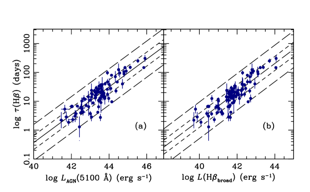
Figure 1: Panel (a): The rest-frame H$\beta$ lag in days is shown as a function of the AGN luminosity $L_{\rm AGN}(5100\,{\rm\AA})$ in erg s^-1. The host-galaxy starlight contribution has been removed by using unsaturated HST  images (see Bentz et al. 2013). Panel (b): The H$\beta$ lag in days is shown as a function of the broad H$\beta$ luminosity $L(\mbox{\rm H$\beta$}_{\rm broad})$ in erg s^-1. The narrow component of H$\beta$ has been removed in each case where it was sufficiently strong (i.e., easily identifiable) to isolate. In both panels, the solid line shows the best-fit to the data using equation (10) with coefficients given in Table 2. The short dashed lines show the $\pm 1\,\sigma$ uncertainty (equivalent to enclosing 68% of the values for a Gaussian distribution) and the long dashed lines show the $2.6\sigma$ uncertainties (equivalent to enclosing 99% of the values for a Gaussian distribution). The Spearman rank correlation coefficient for the data in panel (a) is $\rho=0.797$ and the probability that the relationship arises by chance is $P<10^{-6}$, and for the data in panel (b), $\rho=0.873$ with $P<10^{-6}$.

Table 2: Radius–Luminosity and Luminosity–Luminosity Relations

Line	$x$	$y$	$a\pm\Delta a$	$b\pm\Delta b$	$x_{0}$	$\varepsilon_{y}$	$\Delta$	Figure
(1)	(2)	(3)	(4)	(5)	(6)	(7)	(8)	(9)
1	$\log L_{\scriptsize\rm AGN}(5100\,{\rm\AA})$	$\log\tau(\mbox{\rm H$\beta$})$	$1.228\pm 0.025$	$0.482\pm 0.029$	$43.444$	$0.213\pm 0.021$	$0.241$	1a
2	$\log L(\mbox{\rm H$\beta$}_{\scriptsize\rm broad})$	$\log\tau(\mbox{\rm H$\beta$})$	$1.200\pm 0.025$	$0.492\pm 0.030$	$41.746$	$0.218\pm 0.022$	$0.244$	1b
3	$\log L(1350\,{\rm\AA})$	$\log\tau(\mbox{\rm C\,{\sc iv}})$	$1.915\pm 0.047$	$0.517\pm 0.036$	$45.351$	$0.336\pm 0.041$	$0.361$	7
4	$\log L_{\scriptsize\rm AGN}(5100\,{\rm\AA})$	$\log L(\mbox{\rm H$\beta$}_{\rm broad})$	$41.797\pm 0.017$	$0.960\pm 0.020$	$43.444$	$0.158\pm 0.014$	$0.171$	2
5	$\log L(\mbox{\rm H$\beta$}_{\rm broad})$	$\log L_{\scriptsize\rm AGN}(5100\,{\rm\AA})$	$43.396\pm 0.018$	$1.003\pm 0.022$	$41.746$	$0.161\pm 0.015$	$0.174$	2

Accounting for the host-galaxy contribution in the same way for large number of AGNs, such as those in SDSS-RM (not to mention the entire SDSS catalog), is simply not feasible. It is well-known, however, that there is a tight correlation between the AGN continuum luminosity and the luminosity of H$\beta$ (e.g., Yee 1980; Ilić et al. 2017), and it has indeed been argued that the H$\beta$ emission-line luminosity can be used as a proxy for the AGN continuum luminosity for reverberation studies (Kaspi et al. 2005; Vestergaard & Peterson 2006; Greene et al. 2010). However, in some of the reverberation-mapped sources, narrow-line H$\beta$ contributes significantly to the total H$\beta$ flux; NGC 4151 is an extreme example (e.g., Antonucci & Cohen 1983; Bentz et al. 2006a; Fausnaugh et al. 2017). Whenever the narrow-line component can be isolated, it has been subtracted from the total H$\beta$ flux. This also affects the line-width measurements. In general, it is assumed that [O iii] $\lambda 5007$ can be used as a template for narrow H$\beta$. The template is shifted and scaled to the largest flux that, when subtracted from the spectrum, does not produce a depression at the center of the remaining broad H$\beta$ component. In Figure 2, we show the tight relationship between $L_{\rm AGN}(5100\,{\rm\AA})$ and $L(\mbox{\rm H$\beta$}_{\rm broad})$; the best-fit coefficients for this relationship are given in Table 2.

In panel (b) of Figure 1, we show the H$\beta$ lag as a function of the luminosity of the broad component of H$\beta$, with the narrow component removed whenever possible. We give the best-fit values to the equation (10) in the second row of Table 2, which shows that the slope of this relationship is nearly identical to the slope of the $R$–$L$ relationship using the AGN continuum. The luminosity of the H$\beta$ broad component is thus an excellent proxy for the AGN luminosity and requires only removal of the H$\beta$ narrow component (at least when it is significant) which is much easier than estimating the starlight contribution to the continuum luminosity at 5100 Å. Moreover, by using the line flux instead of the continuum flux, we can include core-dominated radio sources where the continuum may be enhanced by the jet component (Greene & Ho 2005). This is therefore the $R$–$L$ relationship we prefer for the purpose of estimating single-epoch masses and we will focus on this relationship through the remainder of this contribution.

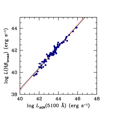
Figure 2: The relationship between the broad H$\beta$ emission line luminosity and the starlight-corrected AGN luminosity for the sources in Table A1. The black solid line is the regression of $L(\mbox{\rm H$\beta$}_{\rm broad})$ on $L_{\rm AGN}(5100\,{\rm\AA})$; the Spearman rank coefficient for this fit is $\rho=0.901$ with $P<10^{-6}$. The red dotted line is the regression of $L_{\rm AGN}(5100\,{\rm\AA})$ on $L(\mbox{\rm H$\beta$}_{\rm broad})$, which we use in equation (24); for this fit $\rho=0.970$ and $P<10^{-6}$. The coefficients for both fits are given in Table 2.

3.2 Line-Width Relationships

We now consider the use of $\sigma_{\rm M}$ and ${\rm FWHM}_{\rm M}$ as proxies for $\sigma_{\rm R}$ (cf. Collin et al. 2006; Wang et al. 2019). Panel (a) of Figure 3 shows the relationship between $\mbox{$\sigma_{\rm R}$}(\mbox{\rm H$\beta$})$, the H$\beta$ line dispersion in the rms spectrum, and $\mbox{$\sigma_{\rm M}$}(\mbox{\rm H$\beta$}),$ the H$\beta$ line dispersion in the mean spectrum. The relationship is nearly linear (slope $=1.085\pm 0.045$) and the intrinsic scatter is small ($0.079$ dex). The fit coefficients are given in the first line of Table 3.

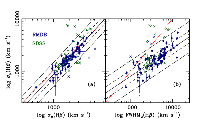
Figure 3: The relationship between H$\beta$ line dispersion in the rms $\mbox{$\sigma_{\rm R}$}(\mbox{\rm H$\beta$})$ and mean $\mbox{$\sigma_{\rm M}$}(\mbox{\rm H$\beta$})$ spectra is shown in panel (a). The relationship between H$\beta$ line dispersion in the rms spectrum $\sigma_{\rm R}$(H$\beta$) and FWHM in the mean spectrum ${\rm FWHM}_{\rm M}$(H$\beta$) is shown in panel (b). Blue filled circles are for the RMDB sample (Table A1) and open green triangles are for the SDSS sample (Table A3). The solid lines are best fits to equation (10) with coefficients in Table 3. The short dashed and long dashed lines indicate the $\pm 1\sigma$ and $\pm 2.6\sigma$ envelopes, respectively, and the red dotted lines indicate where the two line-width measures are equal. Crosses are points that were rejected at the 2.6$\sigma$ (99%) level and are colored-coded like the circles. The relationship in panel (a) is nearly linear (slope $=1.085\pm 0.045$) and the scatter $\varepsilon_{y}$ is low (0.079 dex). The Spearman rank correlation coefficient for these data is $\rho=0.901$ and the probability of the correlation arising by chance is $P<10^{-6}.$ It is clear in panel (b) that ${\rm FWHM}_{\rm M}$(H$\beta$) and $\sigma_{\rm R}$(H$\beta$) are well-correlated, but the relationship is significantly non-linear (slope $=0.535\pm 0.042$), the scatter $\varepsilon_{y}$ is slightly larger (0.106 dex), and there are several significant outliers. For these data, $\rho=0.786$ and $P<10^{-6}.$

Table 3: Line-Width Relations

Line	$x$	$y$	$a\pm\Delta a$	$b\pm\Delta b$	$x_{0}$	$\varepsilon_{y}$	$\Delta$	Figure
(1)	(2)	(3)	(4)	(5)	(6)	(7)	(8)	(9)
1	$\log\mbox{$\sigma_{\rm M}$}(\mbox{\rm H$\beta$})$	$\log\mbox{$\sigma_{\rm R}$}(\mbox{\rm H$\beta$})$	$3.260\pm 0.008$	$1.085\pm 0.045$	3.297	$0.079\pm 0.006$	0.087	3a
2	$\log\mbox{${\rm FWHM}_{\rm M}$}(\mbox{\rm H$\beta$})$	$\log\mbox{$\sigma_{\rm R}$}(\mbox{\rm H$\beta$})$	$3.205\pm 0.011$	$0.535\pm 0.042$	3.559	$0.106\pm 0.001$	0.114	3b
3	$\log\mbox{$\sigma_{\rm M}$}(\mbox{\rm C\,{\sc iv}})$	$\log\mbox{$\sigma_{\rm R}$}(\mbox{\rm C\,{\sc iv}})$	$3.436\pm 0.009$	$0.822\pm 0.059$	3.394	$0.064\pm 0.008$	0.067	8a
4	$\log\mbox{${\rm FWHM}_{\rm M}$}(\mbox{\rm C\,{\sc iv}})$	$\log\mbox{$\sigma_{\rm R}$}(\mbox{\rm C\,{\sc iv}})$	$3.447\pm 0.016$	$0.445\pm 0.101$	3.580	$0.121\pm 0.014$	0.121	8b

We also show in panel (a) of Figure 3 the relationship between $\sigma_{\rm R}$(H$\beta$) and the FWHM of H$\beta$ in the mean spectrum, ${\rm FWHM}_{\rm M}$(H$\beta$). The fit coefficients are given in the second line of Table 3. The relationship is far from linear (slope $=0.535\pm 0.042$), and the scatter $\varepsilon_{y}$ is larger than it is for the $\sigma_{\rm R}$(H$\beta$)–$\sigma_{\rm M}$(H$\beta$) relationship, even after removal of the notable outliers. The shallow slope of the relationship between ${\rm FWHM}_{\rm M}$ and $\sigma_{\rm R}$ is why the mass distribution is stretched by using ${\rm FWHM}_{\rm M}$ as the line-width measure in equation (2): for any given $R$, the ratio $(\mbox{${\rm FWHM}_{\rm M}$}/\mbox{$\sigma_{\rm R}$})^{2}$ is larger at the high-mass end of the distribution than it is at the low-mass end. Use of ${\rm FWHM}_{\rm M}$ in equation (2) overestimates the high masses and underestimates the low masses. While it is clear that $\sigma_{\rm M}$(H$\beta$) is an excellent proxy for $\sigma_{\rm R}$(H$\beta$), the value of ${\rm FWHM}_{\rm M}$(H$\beta$) is less clear, though the shallow slope of the ${\rm FWHM}_{\rm M}$–$\sigma_{\rm R}$ relationship needs to be taken into account. We will fit both versions in order to understand the relative merits of each.

3.3 Single-Epoch Predictors of the Virial Product

In the previous subsections, we have re-established the correlations between $\tau(\mbox{\rm H$\beta$})$ and $L(\mbox{\rm H$\beta$}_{\rm broad})$ and between $\sigma_{\rm R}$(H$\beta$) and both $\sigma_{\rm M}$(H$\beta$) and ${\rm FWHM}_{\rm M}$(H$\beta$). As a first approximation for a formula to estimate single-epoch masses, we fit the following equations:

$$\log\mbox{$\mu_{\rm RM}$}(\mbox{\rm H$\beta$})=a+b\left[\log L(\mbox{\rm H$\beta$}_{\rm broad})-x_{0}\right]+c\left[\log\mbox{$\sigma_{\rm M}$}(\mbox{\rm H$\beta$})-y_{0}\right],$$ (16)

and

$$\log\mbox{$\mu_{\rm RM}$}(\mbox{\rm H$\beta$})=a+b\left[\log L(\mbox{\rm H$\beta$}_{\rm broad})-x_{0}\right]+c\left[\log\mbox{${\rm FWHM}_{\rm M}$}(\mbox{\rm H$\beta$})-y_{0}\right].$$ (17)

The results of these fits based on the combined RMDB data (Table A1) and SDSS data (Table A3) are given in the first two lines of Table 4, and illustrated in panels (a) and (b) of Figure 4. Using these coefficients, we have initial of predictors of $\log\mbox{$\mu_{\rm SE}$}(\mbox{\rm H$\beta$})$ using $\sigma_{\rm M}$ as the line-width measure,

$$\log\mbox{$\mu_{\rm SE}$}(\mbox{\rm H$\beta$})=6.975+0.566\left[\log L(\mbox{\rm H$\beta$}_{\rm broad})-41.857\right]+1.757\left[\log\mbox{$\sigma_{\rm M}$}(\mbox{\rm H$\beta$})-3.293\right],$$ (18)

and using ${\rm FWHM}_{\rm M}$ as the line-width measure,

$$\log\mbox{$\mu_{\rm SE}$}(\mbox{\rm H$\beta$})=6.981+0.587\left[\log L(\mbox{\rm H$\beta$}_{\rm broad})-41.857\right]+1.039\left[\log\mbox{${\rm FWHM}_{\rm M}$}(\mbox{\rm H$\beta$})-3.599\right].$$ (19)

The luminosity coefficient $b$ and the line-width coefficient $c$ are roughly as expected from the virial relationship and the $R$–$L$ relationship, and we note that the line-width coefficient for ${\rm FWHM}_{\rm M}$ ($c=1.039$) is much smaller than that of $\sigma_{\rm M}$ ($c=1.757$), as expected from Figure 3. It is clear that both equations (18) and (19) overestimate masses at the low end and underestimate them at the high end, thus biasing the prediction. Coefficients based on fits to the relationship between $\log\mbox{$\mu_{\rm SE}$}(\mbox{\rm H$\beta$})$ and $\log\mbox{$\mu_{\rm RM}$}(\mbox{\rm H$\beta$})$ are given in the top two rows of Table 5, and the fits are shown in panels (a) and (b) of Figure 4. In both cases, the slopes are too shallow. The failure of equations (18) and (19) to correctly recover $\log\mbox{$\mu_{\rm RM}$}(\mbox{\rm H$\beta$})$ suggests that another parameter is required for the single-epoch virial product prediction.

We investigated the possible importance of another parameter by plotting the residuals $\Delta\log\mu=\log\mbox{$\mu_{\rm RM}$}-\log\mbox{$\mu_{\rm SE}$}$ against other parameters, specifically luminosity, mass (virial product), Eddington ratio, emission-line lag, and both line width and line-width ratio ${\rm FWHM}/\mbox{$\sigma_{\rm line}$}$ for both mean and rms spectra. The most significant correlation between the virial product residuals and other parameters was for Eddington ratio, which has been a result of other recent investigations (Du et al. 2016; Grier et al. 2017b; Du et al. 2018; Du & Wang 2019; Martínez-Aldama et al. 2019; Fonseca Alvarez et al. 2020). To determine the Eddington ratio, we start with the Eddington luminosity

$$L_{\rm Edd}=\frac{4\pi Gcm_{e}M}{\sigma_{e}}=1.257\times 10^{38}\left(\frac{M}{\mbox{$M_{\odot}$}}\right),$$ (20)

where $m_{e}$ is the electron mass and $\sigma_{e}$ is the Thomson cross-section. The black hole mass is $\log M=\log f+\log\mu$ and, as explained in the Appendix, we assume $\log f=0.683\pm 0.150$ (Batiste et al. 2017) so the Eddington luminosity is

$$\log L_{\rm Edd}=\log f+38.099+\log\mbox{$\mu_{\rm RM}$}=38.782+\log\mbox{$\mu_{\rm RM}$}.$$ (21)

The bolometric luminosity can be obtained from the observed 5100 Å AGN luminosity plus a bolometric correction

$$\log L_{\rm bol}=\log L_{\rm AGN}(5100\,{\rm\AA})+\log k_{\rm bol}.$$ (22)

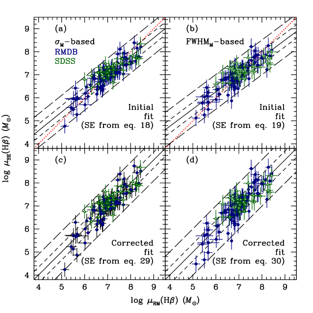
Figure 4: Single-epoch H$\beta$-based virial product predictions using equations (18) and (19) in panels (a) and (b), respectively, compared with the actual RM measurements for the same sources. The coefficients and their uncertainties for these initial predictors of $\log\mbox{$\mu_{\rm SE}$}(\mbox{\rm H$\beta$})$ are presented in the first two lines of Table 4. Blue filled circles represent RMDB data (Table A1) and green open triangles represent SDSS data (Table A3). The solid line shows the best fit to the data, and the red dotted line shows where the two values are equal. Coefficients for fits to the $\log\mbox{$\mu_{\rm SE}$}(\mbox{\rm H$\beta$})$–$\log\mbox{$\mu_{\rm RM}$}(\mbox{\rm H$\beta$})$ relationship are given in the first two lines of Table 5. The short and long dashed lines show the $\pm 1\sigma$ and $\pm 2.6\sigma$ envelopes, respectively. It is clear that this is an inadequate virial product predictor as it systematically underestimates higher masses and overestimates lower masses. The panels (c) and (d) show the same relationship after the empirical corrections as embodied in equations (29) and (30) for $\sigma_{\rm M}$ and ${\rm FWHM}_{\rm M}$, respectively. In panels (c) and (d), the best fit lines cover the equality lines; results of these fits are given in lines 8 and 9 of Table 5. The intrinsic errors $\varepsilon_{y}$ have been added in quadrature to the measurement uncertainties in $\log\mbox{$\mu_{\rm SE}$}(\mbox{\rm H$\beta$})$.

Table 4: Multivariate Fits

Line	$x$	$y$	$z$	$a\pm\Delta a$	$b\pm\Delta b$	$c\pm\Delta c$	$x_{0}$	$y_{0}$	$\varepsilon_{z}$	$\Delta$
	(erg s-1)	(km s-1)	($M_{\odot}$)				(erg s-1)	(km s-1)
(1)	(2)	(3)	(4)	(5)	(6)	(7)	(8)	(9)	(10)	(11)
1	$\log L(\mbox{\rm H$\beta$}_{\rm broad})$	$\log\mbox{$\sigma_{\rm M}$}(\mbox{\rm H$\beta$})$	$\log\mbox{$\mu_{\rm RM}$}(\mbox{\rm H$\beta$})$	$6.975\pm 0.029$	$0.566\pm 0.035$	$1.757\pm 0.160$	$41.857$	$3.293$	$0.273\pm 0.025$	$0.314$
2	$\log L(\mbox{\rm H$\beta$}_{\rm broad})$	$\log\mbox{${\rm FWHM}_{\rm M}$}(\mbox{\rm H$\beta$})$	$\log\mbox{$\mu_{\rm RM}$}(\mbox{\rm H$\beta$})$	$6.981\pm 0.033$	$0.587\pm 0.040$	$1.039\pm 0.128$	$41.857$	$3.559$	$0.323\pm 0.028$	$0.352$
3	$\log L(1350\,{\rm\AA})$	$\log\mbox{$\sigma_{\rm M}$}(\mbox{\rm C\,{\sc iv}})$	$\log\mbox{$\mu_{\rm RM}$}(\mbox{\rm C\,{\sc iv}})$	$7.664\pm 0.039$	$0.599\pm 0.033$	$1.014\pm 0.265$	$44.706$	$3.502$	$0.364\pm 0.033$	$0.397$

Table 5: Initial, Residual, and Final Fits

Line	Data Set	$x$	$y$	$a\pm\Delta a$	$b\pm\Delta b$	$x_{0}$	$\varepsilon_{y}$	$\Delta$	Figure
(1)	(2)	(3)	(4)	(5)	(6)	(7)	(8)	(9)	(10)
	Initial:
1	H$\beta$	$\log\mbox{$\mu_{\rm RM}$}(\mbox{$\sigma_{\rm M}$})$	$\log\mbox{$\mu_{\rm SE}$}(\mbox{$\sigma_{\rm M}$})$	$7.025\pm 0.025$	$0.805\pm 0.038$	$7.041$	$0.249\pm 0.021$	$0.279$	4a
2	H$\beta$	$\log\mbox{$\mu_{\rm RM}$}(\mbox{${\rm FWHM}_{\rm M}$})$	$\log\mbox{$\mu_{\rm SE}$}(\mbox{${\rm FWHM}_{\rm M}$})$	$7.012\pm 0.028$	$0.749\pm 0.042$	$7.007$	$0.278\pm 0.023$	$0.290$	4b
3	C iv	$\log\mbox{$\mu_{\rm RM}$}(\mbox{\rm C\,{\sc iv}})$	$\log\mbox{$\mu_{\rm SE}$}(\mbox{\rm C\,{\sc iv}})$	$7.483\pm 0.033$	$0.787\pm 0.041$	$7.481$	$0.321\pm 0.028$	$0.347$	9a
	Residual:
4	H$\beta$	$\log\dot{m}$	$\Delta\log\mu(\mbox{$\sigma_{\rm M}$})$	$-0.010\pm 0.022$	$-0.422\pm 0.045$	$-0.951$	$0.187\pm 0.021$	$0.246$	5a
5	H$\beta$	$\log\dot{m}$	$\Delta\log\mu(\mbox{${\rm FWHM}_{\rm M}$})$	$-0.007\pm 0.023$	$-0.543\pm 0.046$	$-0.951$	$0.191\pm 0.021$	$0.247$	5b
6	C iv	$\log\dot{m}$	$\Delta\log\mu$	$-0.049\pm 0.026$	$-0.557\pm 0.048$	$-1.155$	$0.213\pm 0.027$	$0.282$	10a
7	C iv	$\log\mbox{$\mu_{\rm RM}$}$	$\Delta\log\mu$	$-0.012\pm 0.026$	$0.297\pm 0.024$	$7.481$	$0.000\pm 0.000$	$0.139$	10d
	Final:
8	H$\beta$	$\log\mbox{$\mu_{\rm RM}$}(\mbox{$\sigma_{\rm M}$})$	$\log\mbox{$\mu_{\rm SE}$}(\mbox{$\sigma_{\rm M}$})$	$7.040\pm 0.031$	$0.999\pm 0.047$	$7.041$	$0.309\pm 0.027$	$0.346$	4c
9	H$\beta$	$\log\mbox{$\mu_{\rm RM}$}(\mbox{${\rm FWHM}_{\rm M}$})$	$\log\mbox{$\mu_{\rm SE}$}(\mbox{${\rm FWHM}_{\rm M}$})$	$7.007\pm 0.037$	$1.000\pm 0.055$	$7.007$	$0.371\pm 0.030$	$0.387$	4d
10	C iv	$\log\mbox{$\mu_{\rm RM}$}(\mbox{\rm C\,{\sc iv}})$	$\log\mbox{$\mu_{\rm SE}$}(\mbox{\rm C\,{\sc iv}})$	$7.485\pm 0.041$	$0.963\pm 0.006$	$7.481$	$0.408\pm 0.035$	$0.439$	9b

We ignore inclination effects and, following Netzer (2019), the bolometric correction we use is

$$\log k_{\rm bol}=10-0.2\log L_{\rm AGN}(5100\,{\rm\AA}).$$ (23)

Since we are using $L(\mbox{\rm H$\beta$}_{\rm broad})$ as a proxy for $L_{\rm AGN}(5100\,{\rm\AA})$, we substitute $L(\mbox{\rm H$\beta$}_{\rm broad})$ for $L_{\rm AGN}(5100\,{\rm\AA})$ by fitting the luminosities in Table A1, yielding (see Table 2)

$$\log L_{\rm AGN}(5100\,{\rm\AA})=43.396+1.003\left[\log L(\mbox{\rm H$\beta$}_{\rm broad})-41.746\right],$$ (24)

so we can write the bolometric luminosity as

$$\log L_{\rm bol}=44.717+0.802\left[\log(\mbox{\rm H$\beta$}_{\rm broad})-41.746\right].$$ (25)

The Eddington ratio $\dot{m}$ is given by

$$\log\mbox{$\dot{m}$}=\log L_{\rm bol}-\log L_{\rm Edd}.$$ (26)

Using equations (25) and (21), the Eddington ratio can then be written as

$$\log\dot{m}=5.935+0.802\left[\log L(\mbox{\rm H$\beta$}_{\rm broad})-41.746\right]-\log\mbox{$\mu_{\rm RM}$}.$$ (27)

To correct the single-epoch masses for Eddington ratio, we fit the equation

$$\Delta\log\mu=\log\mbox{$\mu_{\rm RM}$}-\log\mbox{$\mu_{\rm SE}$}=a+b(\log\dot{m}-x_{0}),$$ (28)

and use this as a correction to our initial fits, equations (18) and (19). The best-fit parameters for comparison of the $\sigma_{\rm M}$ and ${\rm FWHM}_{\rm M}$-based predictors of $\mu_{\rm SE}$ with the reverberation measurements $\mu_{\rm RM}$ are given in lines 4 and 5 of Table 5 and shown in panels (a) and (b) of Figure 5. Combining the correction equation (28) with the best-fit coefficients in Table 5 and equations (18) and (19) yields the corrected single-epoch masses

$$\log\mbox{$\mu_{\rm SE}$}(\mbox{\rm H$\beta$})=6.965+0.566\left[\log L(\mbox{\rm H$\beta$}_{\rm broad})-41.857\right]+1.757\left[\log\mbox{$\sigma_{\rm M}$}(\mbox{\rm H$\beta$})-3.293\right]-0.422\left[\log\mbox{$\dot{m}$}+0.951\right],$$ (29)

and

$$\log\mbox{$\mu_{\rm SE}$}(\mbox{\rm H$\beta$})=6.974+0.587\left[\log L(\mbox{\rm H$\beta$}_{\rm broad})-41.857\right]+1.039\left[\log\mbox{${\rm FWHM}_{\rm M}$}(\mbox{\rm H$\beta$})-3.599\right]-0.543\left[\log\mbox{$\dot{m}$}+0.951\right],$$ (30)

for $\sigma_{\rm M}$ and ${\rm FWHM}_{\rm M}$, respectively.

Once the dependence on Eddington ratio is removed (panels c and b of Figure 4), the residuals do not appear to correlate with other properties. We can now use equations (29) and (30) to make single-epoch mass predictions and we plot these versus the reverberation measurements in panels (c) and (d) of Figure 4. The quality of the correction can be tested by fitting these relationships. The best-fit coefficients for the corrected $\log\mbox{$\mu_{\rm SE}$}(\mbox{\rm H$\beta$})$–$\log\mbox{$\mu_{\rm RM}$}(\mbox{\rm H$\beta$})$ relationship are given in lines 8 and 9 of Table 5.

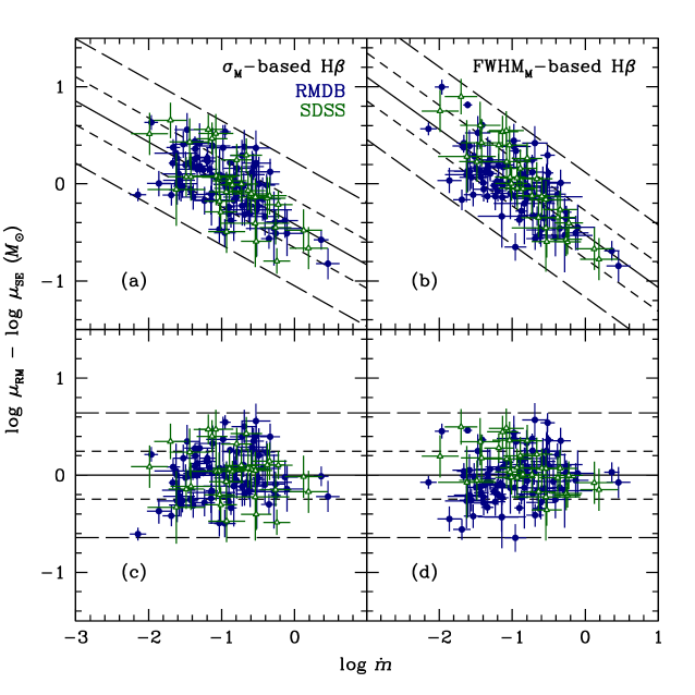
Figure 5: Panel (a): The mass residuals (equation 28) are the difference between the measured reverberation virial products and those predicted by equation (18). The residuals are plotted vs. Eddington ratio $\dot{m}$ (equation 27) for single-epoch virial products based on $\sigma_{\rm M}$(H$\beta$). The Spearman rank correlation coefficient is $\rho=-0.577$ with the probability that the correlation arises by chance $P<10^{-6}.$ Panel (b): The mass residuals (equation 28) are the difference between the measured reverberation virial products and those predicted by equation (19). The residuals are plotted vs. Eddington ratio $\dot{m}$ for single-epoch virial products based on ${\rm FWHM}_{\rm M}$(H$\beta$). For these data, $\rho=-0.679$ with $P<10^{-6}.$ Panels (c) and (d) show residuals after subtraction of the best fit in panels (a) and (b), respectively. The $\varepsilon_{y}$ scatter in the residuals is 0.197 dex for the $\sigma_{\rm M}$-based virial products and 0.204 dex for the ${\rm FWHM}_{\rm M}$-based virial products. In all panels, the solid blue circles represent RMDB data (Table A1) and the open green triangles represent SDSS data (Table A3). The solid line shows the best fit to the data. The short dashed and long dashed lines are the $\pm 1\sigma$ and $\pm 2.6\sigma$ envelopes, respectively. The coefficients of the fits are given in Table 5. Error bars on the residuals are measurement uncertainties only, without systematic errors.

4 Masses Based on C iv

4.1 Fundamental Relationships

As noted in §1, the veracity of C iv-based mass estimates is unclear and remains controversial. The ideal situation would be to have a large number of AGNs with both C iv and H$\beta$ reverberation measurements to effect a direct comparison. There are, unfortunately, very few AGNs that have both; indeed Table A2 of the Appendix includes all C iv results for which there are corresponding H$\beta$ measurements in Table A1. For the few sources with both C iv and H$\beta$ reverberation measurements, we plot the virial products $\mu_{\rm RM}(\mbox{\rm C\,{\sc iv}})$ and $\mu_{\rm RM}(\mbox{\rm H$\beta$})$ in Figure 6; these are in each case a weighted mean value of

$$\mu_{\rm RM}=\left(\frac{c\tau\mbox{$\sigma_{\rm R}$}^{2}}{G}\right)$$ (31)

for each of the observations of H$\beta$ and C iv for the AGNs that appear in both Tables A1 and A2. The close agreement of these values reassures us that the C iv-based RM masses can be trusted, at least over the range of luminosities sampled.

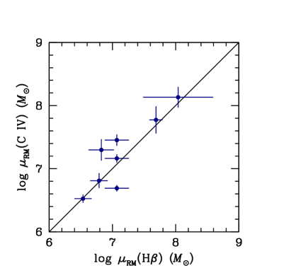
Figure 6: Virial products based on C iv and H$\beta$ for the few cases in the RMDB sample for which both are available. The solid line is the locus where the two virial products are equal. The values are weighted means of $\mbox{$\mu_{\rm RM}$}(\mbox{\rm H$\beta$})$ and $\mbox{$\mu_{\rm RM}$}(\mbox{\rm C\,{\sc iv}})$ for individual AGNs that appear in both Tables A1 and A2. The Spearman rank coefficient for these data is $\rho=0.805$ and the probability that the correlation arises by chance is $P=0.016$.

We now need to consider whether or not luminosities and mean line widths are suitable proxies for emission-line lag and rms line widths in the case of C iv. In Figure 7, we show the relationship between the UV continuum luminosity $L(1350\,{\rm\AA})$ and the C iv emission-line lag $\tau(\mbox{\rm C\,{\sc iv}})$ based on the C iv data in Table A2, plus the SDSS-RM C iv data in Table A4. The coefficients of the fit are given in line 3 of Table 2. We note again that we have removed from the Grier et al. (2019) sample in Table A4 three quasars with BALs, thus reducing the sample size from 48 to 45. The slope of the C iv $R$–$L$ relation ($0.517$) is consistent with that of H$\beta$ ($0.492$), though the $\varepsilon_{y}$ scatter is substantially greater ($0.336$ dex for C iv compared to $0.213$ dex for H$\beta$). Definition of the relationship does not depend on the two separate measurements of very short C iv lag measurements for the dwarf Seyfert NGC 4395 (Peterson et al. 2005). Thus it seems clear that we can use $L(1350\,{\rm\AA})$ as a reasonable proxy for $\tau(\mbox{\rm C\,{\sc iv}})$.

Figure 7: Relationship between the C iv rest-frame emission-line lag $\tau(\mbox{\rm C\,{\sc iv}})$ and the continuum luminosity at 1350 Å. Blue filled circles represent RMDB data (Table A2) and green open triangles represent SDSS data (Table A4). The solid line is the best fit to the data using equation (10) with coefficients given in Table 2. The short dashed and long dashed lines are the $\pm 1\sigma$ and $\pm 2.6\sigma$ envelopes, respectively. The Spearman rank coefficient for these data is $\rho=0.503$ with a probability $P=1.1\times 10^{-5}$ that the correlation arises by chance. If the two lowest luminosity points (both measurements of the dwarf Seyfert NGC 4395) are omitted, the Spearman rank coefficient is decreased to $\rho=0.481$ with $P=1.1\times 10^{-4}$.

We show the relationship between the C iv line dispersion measured in the rms spectrum $\sigma_{\rm R}$(C iv) and the line dispersion in the mean spectrum $\sigma_{\rm M}$(C iv) in Figure 8. The best-fit coefficients are given in line 3 of Table 3. The correlation is good. However, the correlation between ${\rm FWHM}_{\rm M}$(C iv) and $\sigma_{\rm R}$(C iv), also shown in Figure 8 with coefficients in line 4 of Table 3, is rather poor (see also Wang et al. 2020) and demonstrates that ${\rm FWHM}_{\rm M}$(C iv) is a dubious proxy for $\sigma_{\rm R}$(C iv). Measurement of ${\rm FWHM}_{\rm M}$(C iv) is clearly a much less reliable predictor of $\sigma_{\rm R}$(C iv) than is $\sigma_{\rm M}$(C iv), so we will not consider ${\rm FWHM}_{\rm M}$(C iv) further.

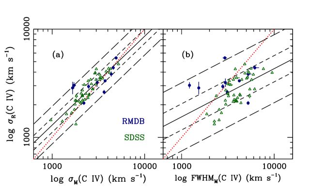
Figure 8: Panel (a): Relationship between C iv line dispersion in the mean and rms spectra of reverberation-mapped AGNs. The Spearman rank coefficient is $\rho=0.873$ with a probability of $P<10^{-6}$ that the correlation arises by chance. Panel (b): Relationship between ${\rm FWHM}_{\rm M}$(C iv) and $\sigma_{\rm R}$(C iv) for reverberation-mapped AGNs. The Spearman rank coefficient for these data is $\rho=0.524$ with $P=3.96\times 10^{-5}$. In both panels, blue filled circles represent RMDB sources in Table A2 and green open triangles represent SDSS-RM sources in Table A4. The red dotted line shows the locus where the two line-width measures are equal. The solid line is the best fit to equation (10) and the coefficients are given in Table 3. The short dashed and long dashed lines show the $\pm 1\sigma$ and $\pm 2.6\sigma$ envelopes, respectively.

4.2 Single-Epoch Masses

Following the same procedures as with H$\beta$, we use the RMDB data (Table A2) and the SDSS-RM data (Table A4) to fit the equation

$$\log\mbox{$\mu_{\rm RM}$}=a+b\left[\log L(1350\,{\rm\AA})-x_{0}\right]+c\left[\log\mbox{$\sigma_{\rm M}$}(\mbox{\rm C\,{\sc iv}})-y_{0}\right].$$ (32)

The resulting fit is shown in Figure 9 and the best-fit coefficients are given in line 3 of Table 4. Thus our initial single-epoch virial product prediction is

$$\log\mbox{$\mu_{\rm SE}$}(\mbox{\rm C\,{\sc iv}})=7.664+0.599\left[\log L(1350\,{\rm\AA})-44.706\right]+1.014\left[\log\mbox{$\sigma_{\rm M}$}(\mbox{\rm C\,{\sc iv}})-3.502\right].$$ (33)

Single-epoch virial product estimates based on equation (33) are plotted against the actual reverberation measurements in Figure 9 and the results of a fit to these data are given in line 3 of Table 5. As was the case with H$\beta$, the slope of this relationship is too shallow, indicating that equation (33) is too simple a prescription and suggesting that another parameter is required.

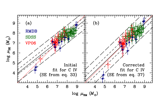
Figure 9: Panel (a): Comparison of single-epoch virial products $\mu_{\rm SE}$(C iv) and reverberation measurements $\mu_{\rm RM}$(C iv) for the data in Table A2 (blue filled circles), the SDSS-RM C iv reverberation data from Table A4 (green open triangles), and data from Table A5 (red open circles). The solid line is the best fit to the data and has slope $0.787\pm 0.041$. As was the case with H$\beta$, masses are overestimated at the low end and underestimated at the high end, excepting the three very low mass measurements. Panel (b): Comparison of single-epoch virial products after empirical correction as given in equation (42). In both panels, the solid line is the best fit to the relationship between $\log\mbox{$\mu_{\rm SE}$}(\mbox{\rm C\,{\sc iv}})$ and $\log\mbox{$\mu_{\rm RM}$}(\mbox{\rm C\,{\sc iv}})$. The short dashed and long dashed lines define the $\pm 1\sigma$ and $\pm 2.6\sigma$ envelopes, respectively. The diagonal red dotted line is the locus where $\mu_{\rm RM}$ and $\mu_{\rm SE}$ are equal. Coefficients for both fits are given in Table 5, in line 3 for panel (a) and in line 10 for panel (b). In both panels, the intrinsic errors $\varepsilon_{y}$ have been added in quadrature to the measurement errors in $\log\mbox{$\mu_{\rm SE}$}(\mbox{\rm C\,{\sc iv}})$.

Guided by our result for H$\beta$, we plot the residuals in $\log\mbox{$\mu_{\rm RM}$}-\log\mbox{$\mu_{\rm SE}$}$ versus Eddington ratio $\dot{m}$ in panel (a) of Figure 10. The Eddington ratio for the UV data is

$$\log\mbox{$\dot{m}$}=-33.737+0.9\log L(1350\,{\rm\AA})-\log\mu_{\rm RM},$$ (34)

where again we have used a bolometric correction from $L(1350\,{\rm\AA})$ from Netzer (2019),

$$\log k_{\rm bol}=5.045-0.1\log L(1350\,{\rm\AA}).$$ (35)

We fitted equation (28) to the C iv mass residuals and Eddington ratio and the results are given in line 6 of Table 5 and also plotted in panel (a) of Figure 10.

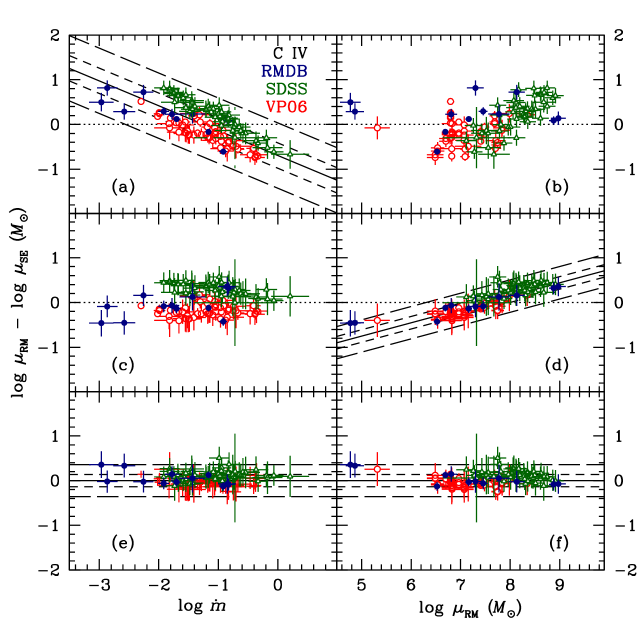
Figure 10: Mass residuals $\Delta\log\mu=\log\mbox{$\mu_{\rm RM}$}-\log\mbox{$\mu_{\rm SE}$}$ versus Eddington rate $\dot{m}$ (left column) and virial product $\mu_{\rm RM}$ (right column) for C iv. Panel (a) shows the residuals between $\mu_{\rm RM}$(C iv) and $\mu_{\rm SE}$(C iv) versus Eddington ratio $\dot{m}$ (equation 26). The fit to these data has Spearman rank coefficient $\rho=-0.693$ with a probability that the correlation arises by chance $P<10^{-6}.$ Panel (b) shows the residuals versus virial product $\mu_{\rm RM}$. Panels (c) and (d) show the residuals versus $\dot{m}$ and $\mu_{\rm RM}$ after subtracting the fit in panel (a). Panel (d) also shows a best fit to the residuals versus mass; coefficients are given in line 7 of Table 5. Note that there is no intrinsic scatter in this relationship because the error bars are so large. For these data, $\rho=0.883$ and $P<10^{-6}.$ Panels (e) and (f) show the mass residuals versus $\dot{m}$ and $\mu_{\rm RM}$ after subtracting the fit in panel (d). The scatter in panels (e) and (f) is 0.138 dex. In all panels, the blue filled circles represent RMDB data (Table A2), the green open triangles are SDSS data (Table A4), and the red open circles are VP06 data (Table A5). Best fits are shown as solid lines and the short dashed and long dashed lines indicate the $\pm 1\sigma$ and $\pm 2.6\sigma$ envelopes, respectively.

The offset between the residuals in the panel (a) of Figure 10 between the RMDB and VP06 data on one hand and the SDSS data on the other might seem to be problematic and we were initially concerned that this might be a data integrity issue. However, upon examining the distribution of mass and luminosity for these three samples as seen in Figure 11, we see clearly that the mass distribution of the SDSS sources is skewed toward much higher values than for the RMDB and VP06 sources, which are relatively local and less luminous than the SDSS quasars. We will thus proceed by examining mass residuals versus both Eddington ratio and $\mu_{\rm RM}$.

Figure 11: Distribution in virial product $\mu_{\rm RM}$ for the RMDB (Table A2, blue solid line), SDSS (Table A3, green dotted line), and VP06 (Table A4, red solid line) samples. The VP06 sample is a subset of the RMDB sample, which is dominated by the relatively low-mass Seyfert galaxies that were the first sources studied by reverberation mapping. The SDSS quasars are comparatively more massive and more luminous.

Figure 10 illustrates the process by which we eliminate the mass residuals in successive iterations. We compute the mass residuals $\Delta\log\mu=\log\mbox{$\mu_{\rm RM}$}-\log\mbox{$\mu_{\rm SE}$}$ from equation (33); these are shown versus $\dot{m}$ (left column) and $\mu_{\rm RM}$ (right column). We fit these residuals versus $\dot{m}$ (panel a) and subtract the best fit to get the corrected residuals shown in the panels (c) and (d). Examination of these residuals as a function of other parameters revealed that they are still correlated with $\mu_{\rm RM}$ (panel d), suggesting that the importance of the Eddington ratio depends on the black hole mass. We therefore fit the residuals a second time, this time as

$$\Delta\log\mu=a+b(\log\mbox{$\mu_{\rm RM}$}\ -x_{0}).$$ (36)

The best fit to this equation is shown in panel (d) and the coefficients are given in Table 5. Subtraction of the best fit yields the residuals shown in panels (e) and (f). We would under most circumstances consider this procedure with some trepidation from a statistical point of view, since $\mu_{\rm RM}$ appears explicitly in one correction and is implicitly in the Eddington ratio. A generalized solution would have multiple degeneracies as both mass and luminosity appear in multiple terms. However, the residual corrections are physically motivated; several previous investigations have also concluded that Eddington ratio is correlated with the deviation from the Bentz et al. (2013) $R$–$L$ relationship, and panels (c) and (d) of Figure 10 suggests that the impact of Eddington ratio varies slightly with mass. Nevertheless, one would prefer to work with parameters that are correlated with or indicators of $\dot{m}$ and $\mu_{\rm RM}$, as we will discuss in §6.

Combining the original fit (equation 33) with the two corrections (equations 34 and 36) yields a corrected single-epoch virial product predictor,

$$\log\mbox{$\mu_{\rm SE}$}(\mbox{\rm C\,{\sc iv}})=7.714+0.761\left[\log L(1350\,{\rm\AA})-44.706\right]+1.289\left[\log\mbox{$\sigma_{\rm M}$}(\mbox{\rm C\,{\sc iv}})-3.502\right].$$ (37)

Single-epoch virial products for all three samples are compared with the reverberation measurements in the right panel of Figure 9. The coefficients of the best fit to these data are given in line 10 of Table 5.

It is worth noting in passing that after correcting for Eddington ratio (Figure 5), the residuals in the H$\beta$-based mass estimates show no correlation with either mass or luminosity.

5 Computing Single-Epoch Masses

To briefly reiterate our approach so far, we started with the assumption that $\mbox{$\mu_{\rm SE}$}=f(R,L)$ only. This proved to be inadequate, so we examined the residuals in the $\log\mbox{$\mu_{\rm SE}$}$–$\log\mbox{$\mu_{\rm RM}$}$ relationship and found that these correlated best with Eddington ratio $\dot{m}$: fundamentally, at increasing $\dot{m}$, the Bentz et al. (2013) $R$–$L$ relationship overpredicts the size of the BLR $R$ (Du & Wang 2019). In the case of C iv, we found additional residuals that correlated with $\mu_{\rm RM}$, although we cannot definitively demonstrate that some part of this is not attributable to inhomogeneities in the data base (a point that will be pursued in the future). While we believe this analysis identifies the physical parameters that affect the mass estimates, there are multiple degeneracies, with both mass and luminosity appearing in more than one term.

Instead of trying to fit coefficients to all the physical parameters that have been identified, we can do a purely empirical correction to equations (16), (17), and (32) since the residuals in the $\log\mbox{$\mu_{\rm RM}$}$–$\log\mbox{$\mu_{\rm SE}$}$ relationships (upper panels in Figure 4 and left panel of Figure 9) are rather small. We can combine the basic $R$–$L$ fits (equations 16, 17, and 32) with the residual fits (equations 28 and 36) to obtain prescriptions that work over the mass range sampled. Renormalizing for convenience, we can estimate single-epoch masses based on H$\beta$($\sigma_{\rm M}$) from

$$\log M_{\rm SE} = \log f+7.530+0.703\left[\log L(\mbox{\rm H$\beta$})-42\right]+2.183\left[\log\mbox{$\sigma_{\rm M}$}(\mbox{\rm H$\beta$})-3.5\right],$$ (38)

with associated uncertainty

$$\Delta\log M_{\rm SE}=\left\{(\Delta\log f)^{2}+\left[0.703\ \Delta\log L(\mbox{\rm H$\beta$})\right]^{2}+\left[2.183\ \Delta\log\mbox{$\sigma_{\rm M}$}(\mbox{\rm H$\beta$})\right]^{2}\right\}^{1/2}\;.$$ (39)

Here $f$ is the scaling factor which is discussed briefly in the Appendix, and $\Delta\log P$ is the uncertainty in the parameter $\log P$. The intrinsic scatter in this relationship is $0.309$ dex, and this must be added in quadrature to the random error. For the case of H$\beta$(${\rm FWHM}_{\rm M}$), a single-epoch mass estimate is obtained from

$$\log M_{\rm SE} = \log f+7.015+0.784\left[\log L(\mbox{\rm H$\beta$})-42\right]+1.387\left[\log\mbox{${\rm FWHM}_{\rm M}$}(\mbox{\rm H$\beta$})-3.5\right],$$ (40)

with associated uncertainty

$$\Delta\log M_{\rm SE}=\left\{(\Delta\log f)^{2}+\left[0.784\ \Delta\log L(\mbox{\rm H$\beta$})\right]^{2}+\left[1.387\ \Delta\log\mbox{${\rm FWHM}_{\rm M}$}(\mbox{\rm H$\beta$})\right]^{2}\right\}^{1/2}\;.$$ (41)

In this case, the intrinsic scatter is $0.371$ dex.

A comparison of the reverberation-based virial products $\mu_{\rm RM}$(H$\beta$) and the single-epoch masses $\mu_{\rm SE}$(H$\beta$) based on equations (38) and (40) is shown in panels (c) and (d) of Figure 4.

Similarly, single-epoch masses based on C iv can be computed from

$$\log M_{\rm SE} = \log f+7.934+0.761\left[\log L(1350\,{\rm\AA})-45\right]+1.289\left[\log\mbox{$\sigma_{\rm M}$}(\mbox{\rm C\,{\sc iv}})-3.5\right],$$ (42)

with associated uncertainty

$$\Delta\log M_{\rm SE}=\left\{(\Delta\log f)^{2}+\left[0.761\ \Delta\log L(1350\,{\rm\AA}\right]^{2}+\left[1.289\ \Delta\log\mbox{$\sigma_{\rm M}$}(\mbox{\rm C\,{\sc iv}})\right]^{2}\right\}^{1/2}\;.$$ (43)

The intrinsic scatter in this relationship is 0.408 dex. Single-epoch predictions and reverberation-based masses for the AGNs in Tables A2, A4, and A5 are compared in panel (b) of Figure 9. Coefficients for this fit are given in line 10 of Table 5.

In Figure 12, we show the distribution in bolometric luminosity and black hole mass based on our prescriptions for the entire sample of SDSS-RM quasars for which H$\beta$ or C iv single-epoch masses can be estimated.

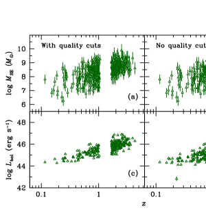
Figure 12: Distribution of masses (panels a and b) and bolometric luminosities (panels c and d) for the entire SDSS-RM sample for which H$\beta$ or C iv single-epoch masses can be computed using equations (38) and (42). Here we assume $f=4.28$ (Batiste et al. 2017). Bolometric corrections were made using equations (23) and (35). In the left column, the quality cuts of §2.1 have been imposed. In the right column, no quality cuts have been made.

6 Discussion

6.1 Single-Epoch Masses

Our primary goal has been to find simple, yet unbiased, prescriptions for estimating the masses of the black holes that power AGNs. Our underlying assumption has been that the most accurate measure of the virial product is given by using the emission-line lag $\tau$ and line width in the rms spectrum $\sigma_{\rm R}$ (e.g., equation A1 in the Appendix) as that quantity produces, upon adjusting by the scaling factor $f$, an $M_{\rm BH}$–$\sigma_{*}$ relationship for AGNs that is in good agreement with that for quiescent galaxies. Given that both $\tau$ and $\sigma_{\rm R}$ average over structure in a complex system (cf. Barth et al. 2015), it is somewhat surprising that this method of mass estimation works as well as it does.

Here we have shown that the luminosity of the broad component of the H$\beta$ emission line is a good proxy for the starlight-corrected AGN luminosity (Figure 1). This is useful since it eliminates the difficult task of accurately modeling the host-galaxy starlight contribution to the continuum luminosity. Moreover, the line luminosity and $\sigma_{\rm R}$ reflect the BLR state at the same time; a measurement of the continuum luminosity, by contrast, better represents the state of the BLR at a time $\tau$ in the future on account of the light travel-time delay within the system (Pogge & Peterson 1992; Gilbert & Peterson 2003; Barth et al. 2015); this is, however, generally a very small effect. For the sake of completeness, we also note that there is a small, but detectable, lag between continuum variations at shorter wavelengths and those at longer wavelengths (McHardy et al. 2014; Shappee et al. 2014; Edelson et al. 2015; Fausnaugh et al. 2016; Edelson et al. 2017; McHardy et al. 2018; Edelson et al. 2019).

We have also confirmed that, for the case of H$\beta$, both $\sigma_{\rm M}$ and ${\rm FWHM}_{\rm M}$ are reasonable proxies for $\sigma_{\rm R}$, though $\sigma_{\rm M}$ is somewhat better than ${\rm FWHM}_{\rm M}$.

On the other hand, the case of C iv remains problematic, as it differs in a number of ways from the other strong emission lines:

1. The equivalent width of C iv decreases with luminosity, which is known as the Baldwin Effect (Baldwin 1977); C iv is driven by higher-energy photons than, say, the Balmer lines and the Baldwin Effect reflects a softening of the high-ionization continuum. This could be due to higher Eddington ratio (Baskin & Laor 2004) or because more massive black holes have cooler accretion disks (Korista, Baldwin, & Ferland 1998).

2. The C iv emission line is typically blueshifted with respect to the systemic redshift of the quasar, which is attributed to outflow of the BLR gas (Gaskell 1982; Wilkes 1984, 1986; Espey et al. 1989; Wills et al. 1993; Richards et al. 2002; Sulentic et al. 2007; Richards et al. 2011; Coatman et al. 2016; Shen 2016; Bisogni et al. 2017; Vietri et al. 2018).

3. BALs in the short-wavelength wing of C iv, another signature of outflow, are common (Weymann et al. 1991; Hall et al. 2002; Hewett & Foltz 2003; Allen et al. 2011). We remind the reader that in §2.1 we removed $\sim 17$% of our SDSS C iv sample because the presence of BALs precludes accurate line-width measurements.

4. The pattern of “breathing” in C iv is the opposite of what is seen in H$\beta$ (Wang et al. 2020). Breathing refers to the response of the emission lines, both lag and line width, to changes in the continuum luminosity. In the case of H$\beta$, an increase in luminosity produces an increase in lag and a decrease in line width (Gilbert & Peterson 2003; Goad, Korista, & Knigge 2004; Cackett & Horne 2006). In the case of C iv, however, the line width increases when the continuum luminosity increases, contrary to expectations from the virial theorem (equation 2).

We must certainly be mindful that outflows can affect a mass measurement, though the effect is small if the gas is at escape velocity. Notably, in the cases studied to date there is good agreement between H$\beta$-based and C iv-based virial products (Figure 7), though, again, these are local Seyfert galaxies that are not representative of the general quasar population.

The C iv breathing issue is addressed in detail by Wang et al. (2020), building on evidence for a non-reverberating narrow core or blue excess in the C iv emission line presented by Denney (2012). In this two-component model, the variable part of the line is much broader than the non-variable core. As the continuum brightens, the variable broad component increases in prominence, resulting in a larger value of $\sigma_{\rm M}$. As the broad component reverberates in response to continuum variations, $\sigma_{\rm M}$ will track $\sigma_{\rm R}$ much better than ${\rm FWHM}_{\rm M}$, thus explaining the breathing characteristics and why ${\rm FWHM}_{\rm M}$ is a poor line-width measure for estimating black hole masses. Physical interpretation of the non-varying core remains an open question: Denney (2012) suggests that it might be an optically thin disk wind or an inner extension of the narrow-line region.

6.2 Eigenvector 1 and the Role of Eddington Ratio

Aside from the Baldwin Effect (Baldwin 1977), the average spectra of quasars show little dependence on luminosity (e.g., Vanden Berk et al. 2004). However, individual objects show considerable spectral diversity or differences from the mean spectrum, regardless of luminosity. Many of these spectral differences show strong correlations and anticorrelations with other spectral properties or physical parameters as revealed by Principal Component Analysis (PCA), as first shown by Boroson & Green (1992). The strongest of these multiple correlations, Eigenvector 1, is most clearly characterized by the anticorrelation between (a) the strength of the Fe ii $\lambda 4570$ and Fe ii $\lambda\lambda 5190$, 5320 complexes on either side of the broad H$\beta$ complex and (b) the strength of the [O iii] $\lambda\lambda 4959$, 5007 doublet. The Fe ii strength is typically characterized by the ratio of the equivalent widths (EW) or fluxes of Fe ii to H$\beta$, i.e., $\mbox{${\cal R}$(Fe\,{\sc ii})}={\rm EW(\mbox{\rm Fe\,{\sc ii}})}/{\rm EW(\mbox{\rm H$\beta$})}$. Boroson & Green (1992) speculate that the physical driver behind Eigenvector 1 is Eddington ratio as they are able to argue against inclination effects. Sulentic et al. (2000) incorporate UV data into the PCA and found that the magnitude of the C iv emission-line blueshift, a ubiquitous feature of AGN UV spectra (e.g., Richards et al. 2002), is also an Eigenvector 1 component, with larger blueshifts associated with higher ${\cal R}$(Fe ii) and lower [O iii] strength. This has been confirmed in a number of subsequent studies (Baskin & Laor 2005; Coatman et al. 2016; Sulentic et al. 2017). Sulentic et al. (2000) also demonstrated that the “narrow-line Seyfert 1” (NLS1) galaxies (Osterbrock & Pogge 1985), a subset of Type 1 AGNs with particularly small broad-line widths (${\rm FWHM}(\mbox{\rm H$\beta$})<2000\,\mbox{\rm km~{}s${}^{-1}$}$), lie at the strong ${\cal R}$(Fe ii)–weak [O iii] extreme of Eigenvector 1. To see why this is so, if we combine the $R$–$L$ relation with eq. (2), the expected line width dependence is seen to be

$$V\propto\left(\frac{M}{L^{1/2}}\right)^{1/2}\propto\left(\frac{M}{\mbox{$\dot{m}$}}\right)^{1/4},$$ (44)

where $\mbox{$\dot{m}$}\propto L/M$ is the Eddington ratio (eq. 26). Thus AGNs with the highest Eddington ratios have the smallest broad-line widths, and many such sources are classified as NLS1s. Boroson (2002) argues that the physical parameter driving Eigenvector 1 is indeed Eddington ratio, and that Eigenvector 2 is driven by accretion rate; these two physical parameters, plus inclination, appear to account for most of the spectral diversity among quasars. There is now, we believe, general consensus in the literature that Eigenvector 1 is driven by Eddington ratio (e.g., Shen & Ho 2014; Sun & Shen 2015; Marziani et al. 2018), and our own analysis supports this.

The necessity of including an Eddington ratio correction to single-epoch mass estimators became an issue when poor argeement was found between H$\beta$ and Mg ii-based SE masses on one hand and C iv-based masses on the other. Shen et al. (2008b) found that the offset between Mg ii-based SE masses and those based on C iv correlated with the C iv blueshift, an Eigenvector 1 parameter as already noted, thus enabling an empirical correction. Similarly Runnoe et al. (2013a) and Brotherton et al. (2015a) use the strength of the Si iv-O iv] blend, another Eigenvector 1 parameter, to effect an empirical correction.

The Super-Eddington Accreting Massive Black Holes (SEAMBH) collaboration has focused on high-$\dot{m}$ candidates in their reverberation-mapping program (Du et al. 2014, 2016, 2018; Du & Wang 2019). An important result from these studies, as we have noted earlier, is that the H$\beta$ lags are smaller than predicted by the current state-of-the-art $R$–$L$ relationship (Bentz et al. 2013). This implies that in these objects the ratio of hydrogen-ionizing photons to optical photons is lower than in the lower $\dot{m}$ sources; this is also consistent with the relative strength of ${\cal R}$(Fe ii), the weakness of high-ionization lines such as [O iii], and the soft X-ray spectra (Boller, Brandt, & Fink 1996) of high $\dot{m}$  sources. Du & Wang (2019) choose to make their correction to the BLR radius through adding a term that correlates with the deficiency of ionizing photons. In our approach, we absorb the correction directly into the virial product computation.

The studies cited above have noted that an Eddington ratio correction is required for single-epoch masses based on H$\beta$. We find, as have others (Shen et al. 2008b; Bian et al. 2012; Shen & Liu 2012; Runnoe et al. 2013a; Brotherton et al. 2015a; Coatman et al. 2017), that a similar correction is required for C iv-based masses as well.

As noted in §4.2, from a statistical point of view, in the single-epoch mass equations it would be preferrable to replace the Eddington ratio with a parameter strongly correlated with it. However, we find that the scatter in these relationships is so large that any gain in the accuracy of black hole mass estimates is offset by a large loss of precision. For example, while the correlation between ${\cal R}$(Fe ii) and Eddington ratio exists, as shown for the SDSS-RM sample in Figure 13, the scatter is so large that the correlation has no real predictive power. We therefore elect at this time to focus on the empirical formulae given in §5.

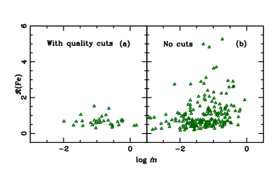
Figure 13: Correlation between ${\cal R}{\rm(Fe)}$ and Eddington ratio $\dot{m}$ for the subset of SDSS-RM quasars selected for our study on the basis of quality cuts (§2.1) in panel (a) and for all SDSS-RM quasars with measured Fe ii equivalent widths in the compilation of Shen et al. (2019) in panel (b). The Eddington ratio used by Shen et al. (2019) differs slightly from that used here.

6.3 Future Improvements

While we believe our current single-epoch prescription for estimating quasar black hole masses is more accurate than previous prescriptions, we also recognize that there are additional improvements that can be made to improve both accuracy and precision, some of which we became aware of near the end of the current project. We intend to implement these in the future. Topics that we will investigate in the future include the following:

1. Replace those reverberation lag measurements made with the interpolated cross-correlation function (Gaskell & Peterson 1987; White & Peterson 1994; Peterson et al. 1998b, 2004) with lag measurements and uncertainties from JAVELIN (Zu, Kochanek, & Peterson 2011). Recent tests (Li et al. 2019; Yu et al. 2020) show that while the JAVELIN and interpolation cross-correlation lags are generally consistent, the uncertainties predicted by JAVELIN are more reliable.

2. Utilize the expanded SDSS-RM database, which now extends over six years, not only to make use of additional lag detections, but to capitalize on the gains in $S/N$ that will increase the overall quality of the lag and line-width measurements and result in fewer rejections of poor data.

3. Expand the database in Table A1 with recent results and other previous results that we excluded because they did not have starlight-corrected continuum luminosities.

4. Update the VP06 database used to produce Table A5. There are now additional reverberation-mapped AGNs with archived HST UV spectra. Some of the poorer data in Table A5 can be replaced measurements based on higher-quality spectra.

5. Consider use of other line-width measures that may correlate well with $\sigma_{\rm line}$, but are less sensitive to blending in the wings. Mean absolute deviation (MAD) is one such candidate; indeed, Park et al. (2017) have already demonstrated that C iv-based masses are more consistent with those based on other lines if either $\sigma_{\rm line}$ or MAD is used instead of FWHM to characterize the line width.

6. Improve line-width measurements. There appear to be some systematic differences among the various data sets, probably due to different processes for measuring $\sigma_{\rm M}$; for example, panels (e) and (f) of Figure 10 show that the SE mass estimates for the VP06 sample are slightly higher than those from SDSS (compare also the last two columns in Table A5). Work on deblending alogrithms would aid more precise measurement of $\sigma_{\rm M}$, in particular.

7 Summary

The main results of this paper are:

1. We confirm that the luminosity of the broad component of the H$\beta$ emission line $L(\mbox{\rm H$\beta$}_{\rm broad})$ is an excellent substitute for the AGN continuum luminosity $L_{\rm AGN}(5100\,{\rm\AA})$ for predicting the H$\beta$ emission-line reverberation lag $\tau(\mbox{\rm H$\beta$})$. It has the advantage of being easier to isolate than $L_{\rm AGN}(5100\,{\rm\AA})$, which requires an accurate estimate of the host-galaxy starlight contribution to the observed luminosity. The fact that there is no statistical penalty for using $L(\mbox{\rm H$\beta$})$ as the luminosity measure is, from a practical point of view, one of the most important findings of this work because the high-quality unsaturated space-based images that are used for host-galaxy modeling (see Bentz et al. 2013, and references therein) may not be so easily acquired in the future.

2. We confirm that the line dispersion of the H$\beta$ broad component $\sigma_{\rm M}$(H$\beta$) and the full-width at half maximum for the H$\beta$ broad component ${\rm FWHM}_{\rm M}$(H$\beta$) in mean, or single-epoch, spectra are both reasonable proxies for the line dispersion of H$\beta$ in the rms spectrum $\sigma_{\rm M}$(H$\beta$) for computing single-epoch virial products $\mu_{\rm SE}$(H$\beta$). We find that $\sigma_{\rm M}$(H$\beta$) gives better results than ${\rm FWHM}_{\rm M}$(H$\beta$), but both are usable.

3. In the case of C iv, we find that the line dispersion of the C iv emission line $\sigma_{\rm M}$(C iv) in the mean, or single-epoch, spectrum is a good proxy for the line dispersion in the rms spectrum $\sigma_{\rm R}$(C iv) for estimating single-epoch virial products $\mu_{\rm SE}$(C iv). We find that ${\rm FWHM}_{\rm M}$(C iv), however, does not track $\sigma_{\rm R}$(C iv) well enough to be used as a proxy.

4. Although the $R$–$L$ relationship based on the continuum luminosity $L(1350\,{\rm\AA})$ and C iv emission-line reverberation lag $\tau(\mbox{\rm C\,{\sc iv}})$ is not as well defined as that for H$\beta$, the relationship appears to have a similar slope and it appears to be suitable for estimating virial products $\mu_{\rm SE}$(C iv).

5. We confirm for both H$\beta$ and C iv that combining the reverberation lag estimated from the luminosity with a suitable measurement of the emission-line width together introduces a bias where the high masses are underestimated and the low masses are overestimated. We confirm that the parameter that accounts for the systematic difference between reverberation virial product measurements $\mu_{\rm RM}$ and those estimated using only luminosity and line width is Eddington ratio. Increasing Eddington ratio causes the reverberation radius to shrink, suggesting a softening of the hydrogen-ionizing spectrum.

6. While the virial product estimate from combining luminosity and line width causes a systematic bias, the relationship between the reverberation virial product $\mu_{\rm RM}$ and the single-epoch estimate $\mu_{\rm SE}$ is still a power-law, but with a slope somewhat less than unity (upper panels of Figure 4, left panel of Figure 9). We are therefore able to empirically correct this relationship to an unbiased estimator of $\mu_{\rm SE}$ by fitting the residuals and essentially rotating the power-law distribution to have a slope of unity (lower panels of Figure 4, right panel of Figure 9). We present these empirical estimators for $\mu_{\rm SE}$(H$\beta$) and $\mu_{\rm SE}$(C iv) in §5. On account of its potential utility, we regard this as the most important conclusion of this study.

Database of Reverberation-Mapped AGNs

Reverberation-mapped AGNs provide the fundamental data that anchor the AGN mass scale. We selected all AGNs from the literature (as of 2019 August) for which unsaturated host-galaxy images acquired with HST  are available, since removal of the host-galaxy starlight contribution to the observed luminosity is critical to this calibration, and measurements of H$\beta$ time lags. It is worth noting, however, that since our analysis shows that the broad H$\beta$ flux is a useful proxy for the 5100 Å continuum luminosity, this criterion is over-restrictive and we will avoid imposing it in future compilations. In many cases, there is more than one reverberation-mapping data set available in the literature. In a few cases, the more recent data were acquired to replace, say, a more poorly sampled data set or one for which the initial result was ambiguous for some reason. In other cases, there are multiple data sets of comparable quality for individual AGNs, and in these cases we include them all. The particularly well-studied AGN NGC 5548 has been observed many times and in some sense has served as a “control” source that provides our best information about the repeatability of mass measurements as the continuum and line widths show long-term (compared to reverberation time scales) variations.

The final reverberation-mapped sample for H$\beta$ is given in Table A1. It consists of 98 individual time series for 50 individual low-redshift ($z<0.3$) AGNs. They span a range of AGN luminosity $41.46\leq\log L(5100\,{\rm\AA})\leq 45.81$, in erg s^-1. Luminosities have been corrected for Galactic absorption using extinction values on the NASA Extragalactic Database, which are based on the Schlafly & Finkbeiner (2011) recalibration of the Schlegel, Finkbeiner, & Davis (1998) dust map. Line-width and time-delay measurements are in the rest-frame of the AGNs. Luminosity distances are based on redshift, except the cases noted by Bentz et al. (2013), for which the redshift-independent distances quoted in that paper are used. For two of these sources, NGC 4051 and NGC 4151, we use preliminary Cepheid-based distances (M.M. Fausnaugh, private communication), and for NGC 6814, we use the Cepheid-based distance from Bentz et al. (2019). Individual virial products for these sources are easily computed using the H$\beta$ time lags (Column 6) and line dispersion measurements (Column 12) and the formula

$$\mu=0.1952\left(\frac{\tau(\mbox{\rm H$\beta$})}{{\rm days}}\right)\left(\frac{\mbox{$\sigma_{\rm R}$}(\mbox{\rm H$\beta$})}{{\rm km\,s}^{-1}}\right)^{2}\,\mbox{$M_{\odot}$}.$$ (A1)

Further conversion to mass requires multiplication by the virial factor $f$, i.e. $\log M=\log f+\log\mu$, a dimensionless factor that depends on the inclination, structure, and kinematics of the broad-H$\beta$-emitting region — indeed, detailed modeling of 9 of these objects (Pancoast et al. 2014; Grier et al. 2017a) shows that $f$ depends most clearly on inclination (Grier et al. 2017a). Since such models are available for only a very limited number of AGNs, it is more common to use a statistical estimate of a mean value of $f$ based on a secondary mass indicator, specifically the well-known $M_{\rm BH}$–$\sigma_{*}$ relationship (Ferrarese & Merritt 2000; Gebhardt et al. 2000; Gültekin et al. 2009), where $\sigma_{*}$ is the host-galaxy stellar bulge velocity dispersion. The required assumption is that the AGN $M_{\rm BH}$–$\sigma_{*}$ is identical to that of quiescent galaxies (Woo et al. 2013). In fact, it is found that the $\mu$–$\sigma_{*}$ has a slope consistent with the $M_{\rm BH}$–$\sigma_{*}$ slope for quiescent galaxies (Grier et al. 2013), and the zero points disagree by only a multiplicative factor, which is taken to be $f$. Here we take $\langle\log f\rangle=0.683\pm 0.150$ (Batiste et al. 2017) where the error on the mean is $\Delta\log f=0.030$ — this error must be propagated into the mass measurement error when comparing AGN reverberation-based masses to those based on other methods.

Table A1: Reverberation-Mapped AGNs (H$\beta$)

Source	Ref.	JD Range	$z$	$D_{L}$	$\tau(\mbox{\rm H$\beta$})$	$\log L_{\rm total}(5100)$	$\log L_{\rm AGN}(5100)$	$\log L(\mbox{\rm H$\beta$}_{\rm broad})$	${\rm FWHM}_{\rm M}$(H$\beta$)	$\sigma_{\rm M}$(H$\beta$)	$\sigma_{\rm R}$(H$\beta$)
		($-2400000$)		(Mpc)	(days)	(erg s-1)	(erg s-1)	(erg s-1)	(km s-1)	(km s-1)	(km s-1)
(1)	(2)	(3)	(4)	(5)	(6)	(7)	(8)	(9)	(10)	(11)	(12)
Mrk335	1	49156-49338	0.02579	109.5	$16.8^{+4.8}_{-4.2}$	$43.802\pm 0.010$	$43.703\pm 0.013$	$42.083\pm 0.010$	$1792\pm 3$	$1380\pm 6$	$917\pm 52$
Mrk335	1	49889-50118	0.02579	109.5	$12.5^{+6.6}_{-5.5}$	$43.861\pm 0.010$	$43.777\pm 0.013$	$42.124\pm 0.010$	$1679\pm 2$	$1371\pm 8$	$948\pm 113$
Mrk335	1	55431-55569	0.02579	109.5	$14.3^{+0.7}_{-0.7}$	$43.791\pm 0.007$	$43.683\pm 0.061$	$41.940\pm 0.009$	$1273\pm 3$	$1663\pm 6$	$1293\pm 64$
Mrk1501	2	55430-55568	0.08934	402.5	$12.6^{+3.9}_{-3.9}$	$44.314\pm 0.011$	$43.980\pm 0.053$	$42.719\pm 0.015$	$3106\pm 15$	$3494\pm 35$	$3321\pm 107$
PG0026+129	3	48545-51084	0.14200	653.1	$111.0^{+24.1}_{-28.3}$	$44.977\pm 0.010$	$44.911\pm 0.011$	$42.867\pm 0.016$	$2544\pm 56$	$1738\pm 100$	$1773\pm 285$
PG0052+251	3	48461-51084	0.15445	751.9	$89.8^{+24.5}_{-24.1}$	$44.964\pm 0.013$	$44.791\pm 0.020$	$43.113\pm 0.016$	$5008\pm 73$	$2167\pm 30$	$1783\pm 86$
Fairall9	4	49475-49743	0.04702	202.8	$17.4^{+3.2}_{-4.3}$	$44.224\pm 0.007$	$43.920\pm 0.026$	$42.393\pm 0.007$	$5999\pm 60$	$2347\pm 16$	$3787\pm 197$
Mrk590	1	48090-48323	0.02639	112.1	$20.7^{+3.5}_{-2.7}$	$43.842\pm 0.010$	$43.544\pm 0.029$	$41.855\pm 0.011$	$2788\pm 29$	$1942\pm 26$	$789\pm 74$
Mrk590	1	48848-49048	0.02639	112.1	$14.0^{+8.5}_{-8.8}$	$43.666\pm 0.011$	$43.075\pm 0.073$	$41.522\pm 0.011$	$3729\pm 426$	$2168\pm 30$	$1935\pm 52$
Mrk590	1	49183-49338	0.02639	112.1	$29.2^{+4.9}_{-5.0}$	$43.743\pm 0.010$	$43.320\pm 0.043$	$41.690\pm 0.010$	$2743\pm 79$	$1967\pm 19$	$1251\pm 72$
Mrk590	1	49958-50122	0.02639	112.1	$28.8^{+3.6}_{-4.2}$	$43.865\pm 0.010$	$43.589\pm 0.026$	$41.857\pm 0.010$	$2500\pm 43$	$1880\pm 19$	$1201\pm 130$
3C120	1	47837-50388	0.03301	140.9	$38.1^{+21.3}_{-15.3}$	$44.078\pm 0.012$	$44.010\pm 0.014$	$42.306\pm 0.012$	$2327\pm 48$	$1249\pm 21$	$1166\pm 50$
3C120	5	54726-54920	0.03301	140.9	$27.9^{+7.1}_{-5.9}$	$44.116\pm 0.013$	$44.094\pm 0.013$	$42.453\pm 0.012$	$2386\pm 52$	$\ldots$	$1689\pm 68$
3C120	2	55430-55569	0.03301	140.9	$25.9^{+2.3}_{-2.3}$	$43.993\pm 0.012$	$43.903\pm 0.052$	$42.298\pm 0.015$	$1430\pm 16$	$1687\pm 4$	$1514\pm 65$
Akn120	1	48148-48344	0.03271	139.6	$47.1^{+8.3}_{-12.4}$	$44.254\pm 0.010$	$43.921\pm 0.032$	$42.553\pm 0.010$	$6042\pm 35$	$1753\pm 6$	$1959\pm 109$
Akn120	1	49980-50175	0.03271	139.6	$37.1^{+4.8}_{-5.4}$	$44.131\pm 0.010$	$43.569\pm 0.067$	$42.390\pm 0.010$	$6246\pm 78$	$1862\pm 13$	$1884\pm 48$
MCG+08-11-011	6	56639-56797	0.02048	86.6	$15.72^{+0.50}_{-0.52}$	$43.574\pm 0.009$	$43.282\pm 0.045$	$41.706\pm 0.006$	$1159\pm 8$	$1681\pm 2$	$1466\pm 143$
Mrk6	7	49250-49872	0.01881	80.6	$21.2^{+4.}_{-3.2}$	$43.576\pm 0.009$	$43.351\pm 0.033$	$41.591\pm 0.011$	$\ldots$	$2813\pm 13$	$2836\pm 48$
Mrk6	7	49980-50777	0.01881	80.6	$20.7^{+3.0}_{-2.4}$	$43.578\pm 0.009$	$43.354\pm 0.033$	$41.632\pm 0.010$	$\ldots$	$2804\pm 6$	$2626\pm 37$
Mrk6	7	50869-51516	0.01881	80.6	$20.5^{+5.6}_{-7.0}$	$43.523\pm 0.011$	$43.258\pm 0.042$	$41.584\pm 0.013$	$\ldots$	$2808\pm 14$	$2626\pm 37$
Mrk6	7	51557-53356	0.01881	80.6	$23.9^{+17.0}_{-7.3}$	$43.431\pm 0.007$	$43.070\pm 0.058$	$41.449\pm 0.018$	$\dots$	$2870\pm 13$	$3222\pm 39$
Mrk6	7	53611-54804	0.01881	80.6	$20.4^{+4.6}_{-4.1}$	$43.613\pm 0.005$	$43.413\pm 0.027$	$41.579\pm 0.012$	$\ldots$	$2807\pm 8$	$2864\pm 35$
Mrk6	2	55340-55569	0.01881	80.6	$10.1^{+1.1}_{-1.1}$	$43.719\pm 0.008$	$43.507\pm 0.029$	$41.849\pm 0.012$	$2619\pm 24$	$4006\pm 6$	$3714\pm 68$
Mrk79	1	47838-48044	0.02219	94.0	$9.0^{+8.3}_{-7.8}$	$43.668\pm 0.011$	$43.569\pm 0.014$	$41.818\pm 0.011$	$5056\pm 85$	$2314\pm 23$	$2137\pm 375$
Mrk79	1	48193-48393	0.02219	94.0	$16.1^{+6.6}_{-6.6}$	$43.754\pm 0.010$	$43.675\pm 0.012$	$41.851\pm 0.010$	$4760\pm 31$	$2281\pm 26$	$1683\pm 72$
Mrk79	1	48905-49135	0.02219	94.0	$16.0^{+6.4}_{-5.8}$	$43.695\pm 0.010$	$43.602\pm 0.013$	$41.820\pm 0.010$	$4766\pm 71$	$2312\pm 21$	$1854\pm 72$
Mrk374	6	56663-56795	0.04263	183.3	$14.84^{+5.76}_{-3.30}$	$43.994\pm 0.009$	$43.752\pm 0.036$	$41.764\pm 0.013$	$3250\pm 19$	$1490\pm 4$	$1329\pm 373$
PG0804+761	3	48319-51085	0.10000	447.5	$146.9^{+18.8}_{-18.9}$	$44.905\pm 0.011$	$44.849\pm 0.011$	$43.230\pm 0.012$	$3053\pm 38$	$1434\pm 18$	$1971\pm 105$
NGC2617	6	56639-56797	0.01421	59.8	$4.32^{+1.1}_{-1.35}$	$43.099\pm 0.011$	$42.610\pm 0.096$	$41.173\pm 0.012$	$5303\pm 48$	$2709\pm 6$	$2424\pm 89$
Mrk704	8	55932-55980	0.02923	124.5	$12.65^{+1.49}_{-2.14}$	$43.708\pm 0.005$	$43.517\pm 0.025$	$41.800\pm 0.007$	$3502\pm 31$	$2650\pm 4$	$1860\pm 120$
Mrk110	1	48953-49149	0.03529	150.9	$24.3^{+5.5}_{-8.3}$	$43.711\pm 0.011$	$43.618\pm 0.014$	$42.055\pm 0.011$	$1543\pm 5$	$962\pm 15$	$1196\pm 141$
Mrk110	1	49751-49874	0.03529	150.9	$20.4^{+10.5}_{-6.3}$	$43.771\pm 0.010$	$43.691\pm 0.012$	$41.960\pm 0.010$	$1658\pm 3$	$953\pm 10$	$1115\pm 103$
Mrk110	1	50010-50262	0.03529	150.9	$33.3^{+14.9}_{-10.0}$	$43.594\pm 0.012$	$43.468\pm 0.017$	$41.905\pm 0.012$	$1600\pm 39$	$987\pm 18$	$755\pm 29$
Mrk110	9	51495-51678	0.03529	150.9	$23.4^{+3.6}_{-3.2}$	$43.340\pm 0.007$	$43.225\pm 0.011$	$41.769\pm 0.007$	$\ldots$	$\ldots$	$\ldots$
PG0953+414	3	48319-50997	0.23410	1137.2	$150.1^{+21.6}_{-22.6}$	$45.193\pm.010$	$45.126\pm 0.011$	$43.390\pm 0.012$	$3071\pm 27$	$1659\pm 31$	$1306\pm 144$
NGC3227	10	54184-54269	0.00386	23.7	$3.75^{+0.76}_{-0.82}$	$42.629\pm 0.035$	$42.243\pm 0.068$	$40.387\pm 0.035$	$3972\pm 25$	$1749\pm 4$	$1376\pm 44$
NGC3227	8	55933-56048	0.00386	23.7	$1.29^{+1.56}_{-1.27}$	$42.757\pm 0.006$	$42.424\pm 0.051$	$40.487\pm 0.010$	$1602\pm 2$	$1402\pm 2$	$1368\pm 38$
Mrk142	11	54506-54618	0.04494	193.5	$2.74^{+0.73}_{-0.83}$	$43.709\pm 0.010$	$43.543\pm 0.015$	$41.639\pm 0.010$	$1462\pm 2$	$1116\pm 22$	$859\pm 102$
Mrk142	12	56237-56413	0.04494	193.5	$6.4^{+0.8}_{-2.2}$	$43.610\pm 0.010$	$43.443\pm 0.016$	$41.586\pm 0.010$	$1647\pm 69$	$\ldots$	$\ldots$
NGC3516	14,15	54181-54300	0.00884	37.1	$11.68^{+1.02}_{-1.53}$	$43.299\pm 0.055$	$42.726\pm 0.133$	$40.995\pm 0.057$	$5236\pm 12$	$1584\pm 1$	$1591\pm 10$
NGC3516	8	55932-56072	0.00884	37.1	$5.74^{+2.26}_{-2.04}$	$43.272\pm 0.007$	$42.529\pm 0.196$	$41.022\pm 0.008$	$3231\pm 14$	$2633\pm 3$	$2448\pm 69$
SBS1116+583A	11	54550-54618	0.02787	118.5	$2.31^{+0.62}_{-0.49}$	$42.995\pm 0.021$	$42.076\pm 0.224$	$40.788\pm 0.015$	$3668\pm 186$	$1552\pm 36$	$1528\pm 184$
Arp151	11,13	54506-54618	0.02109	89.2	$3.99^{+0.49}_{-0.68}$	$42.979\pm 0.010$	$42.497\pm 0.047$	$40.931\pm 0.011$	$3098\pm 69$	$2006\pm 24$	$1252\pm 46$
NGC3783	14,15	48607-48833	0.00973	25.1	$10.2^{+3.3}_{-2.3}$	$42.791\pm 0.025$	$42.559\pm 0.051$	$41.009\pm 0.021$	$3770\pm 68$	$1691\pm 19$	$1753\pm 141$
Mrk1310	11	54550-54618	0.01956	82.7	$3.66^{+0.59}_{-0.61}$	$42.937\pm 0.018$	$42.231\pm 0.120$	$40.646\pm 0.012$	$2409\pm 24$	$1209\pm 42$	$755\pm 138$
NGC4051	16	54180-54311	0.00234	15.0	$1.87^{+0.54}_{-0.50}$	$42.290\pm 0.015$	$41.847\pm 0.080$	$40.079\pm 0.018$	$799\pm 2$	$1045\pm 4$	$927\pm 64$
NGC4051	6	56645-56864	0.00234	15.0	$2.87^{+0.86}_{-1.33}$	$42.265\pm 0.005$	$41.732\pm 0.106$	$39.882\pm 0.012$	$765\pm 3$	$470\pm 2$	$493\pm 35$
NGC4151	17	53430-53472	0.00332	15.0	$6.59^{+1.12}_{-0.76}$	$42.549\pm 0.012$	$42.004\pm 0.113$	$40.499\pm 0.013$	$5840\pm 863$	$6158\pm 47$	$2680\pm 64$
NGC4151	6	55931-56072	0.00332	15.0	$6.82^{+0.48}_{-0.57}$	$42.685\pm 0.007$	$42.315\pm 0.060$	$40.956\pm 0.008$	$992\pm 4$	$1833\pm 2$	$1894\pm 9$
Mrk202	11	54550-54617	0.02102	88.9	$3.05^{+1.73}_{-1.12}$	$42.946\pm 0.016$	$42.198\pm 0.126$	$40.477\pm 0.010$	$1471\pm 18$	$867\pm 40$	$659\pm 65$
NGC4253	11	54509-54618	0.01293	54.4	$6.16^{+1.63}_{-1.22}$	$42.948\pm 0.012$	$42.509\pm 0.044$	$40.873\pm 0.010$	$1609\pm 39$	$1088\pm 37$	$\ldots$
PG1226+023	3	48361-50997	0.15834	737.7	$306.80^{+68.5}_{-90.9}$	$45.935\pm 0.011$	$45.907\pm 0.011$	$44.072\pm 0.014$	$3509\pm 36$	$1778\pm 17$	$1777\pm 150$
3C273	18	54795-58194	0.15834	737.7	$146.3^{+8.3}_{-12.1}$	$45.864\pm 0.011$	$45.848\pm 0.011$	$44.056\pm 0.010$	$3256\pm 36$	$1701\pm 15$	$1090\pm 121$
PG1229+204	3	48319-50997	0.06301	274.9	$37.8^{+27.6}_{-15.3}$	$44.053\pm 0.010$	$43.636\pm 0.040$	$42.275\pm 0.011$	$3828\pm 54$	$1608\pm 24$	$1385\pm 111$
NGC4593	19	53391-53580	0.00900	37.7	$3.73^{+0.75}_{-0.75}$	$43.242\pm 0.013$	$43.005\pm 0.035$	$41.237\pm 0.013$	$5143\pm 16$	$1790\pm 3$	$1561\pm 55$
NGC4748	11	54550-54618	0.01463	61.6	$5.55^{+1.62}_{-2.22}$	$43.072\pm 0.012$	$42.557\pm 0.060$	$41.047\pm 0.010$	$1947\pm 66$	$1009\pm 27$	$657\pm 91$
PG1307+085	3	48319-51042	0.15500	718.7	$105.6^{+36.0}_{-46.6}$	$44.849\pm 0.012$	$44.790\pm 0.013$	$43.096\pm 0.020$	$5059\pm 133$	$1963\pm 47$	$1820\pm 122$
MCG-06-30-15	20	55988-56079	0.00775	25.5	$5.33^{+1.86}_{-1.75}$	$42.393\pm 0.009$	$41.651\pm 0.197$	$39.793\pm 0.011$	$1958\pm 75$	$976\pm 8$	$665\pm 87$
NGC5273	21	56774-56838	0.00362	15.3	$2.21^{+1.19}_{-1.60}$	$42.000\pm 0.009$	$41.465\pm 0.106$	$39.702\pm 0.010$	$5688\pm 163$	$1821\pm 53$	$1544\pm 98$
Mrk279	22	50095-50289	0.03045	129.7	$16.7^{+3.9}_{-3.9}$	$43.882\pm 0.021$	$43.643\pm 0.036$	$42.242\pm 0.021$	$5354\pm 32$	$1823\pm 11$	$1420\pm 96$
PG1411+442	3	48319-51038	0.08960	398.2	$124.3^{+61.0}_{-61.7}$	$44.603\pm 0.012$	$44.502\pm 0.014$	$42.792\pm 0.014$	$2801\pm 43$	$1774\pm 29$	$1607\pm 169$
NGC5548	23,24,25	47509-47809	0.01718	72.5	$19.7^{+1.5}_{-1.5}$	$43.534\pm 0.021$	$43.328\pm 0.042$	$41.728\pm 0.018$	$4674\pm 63$	$1934\pm 5$	$1687\pm 56$
NGC5548	24,25	47861-48179	0.01718	72.5	$18.6^{+2.1}_{-2.3}$	$43.390\pm 0.029$	$43.066\pm 0.068$	$41.546\pm 0.029$	$5418\pm 107$	$2227\pm 20$	$1882\pm 83$
NGC5548	24,26	48225-48534	0.01718	72.5	$15.9^{+2.9}_{-2.5}$	$43.496\pm 0.017$	$43.264\pm 0.042$	$41.645\pm 0.026$	$5236\pm 87$	$2205\pm 16$	$2075\pm 81$
NGC5548	24,26	48623-48898	0.01718	72.5	$11.0^{+1.9}_{-2.0}$	$43.360\pm 0.020$	$42.999\pm 0.070$	$41.457\pm 0.030$	$5986\pm 95$	$3110\pm 53$	$2264\pm 88$
NGC5548	24,27	48954-49255	0.01718	72.5	$13.0^{+1.6}_{-1.4}$	$43.497\pm 0.016$	$43.267\pm 0.040$	$41.691\pm 0.016$	$5930\pm 42$	$2486\pm 13$	$1909\pm 129$
NGC5548	24,28	49309-49636	0.01718	72.5	$13.4^{+3.8}_{-4.3}$	$43.509\pm 0.022$	$43.287\pm 0.043$	$41.649\pm 0.022$	$7378\pm 39$	$2877\pm 17$	$2895\pm 114$
NGC5548	24,28	49679-50008	0.01718	72.5	$21.7^{+2.6}_{-2.6}$	$43.604\pm 0.012$	$43.436\pm 0.026$	$41.746\pm 0.013$	$6946\pm 79$	$2432\pm 13$	$2247\pm 134$
NGC5548	24,28	50044-50373	0.01718	72.5	$16.4^{+1.2}_{-1.1}$	$43.527\pm 0.020$	$43.317\pm 0.039$	$41.656\pm 0.018$	$6623\pm 93$	$2276\pm 15$	$2026\pm 68$
NGC5548	24,29	50434-50729	0.01718	72.5	$17.5^{+2.0}_{-1.6}$	$43.413\pm 0.018$	$43.113\pm 0.054$	$41.622\pm 0.015$	$6298\pm 65$	$2178\pm 12$	$1923\pm 62$
NGC5548	24,29	50775-51085	0.01718	72.5	$26.5^{+4.3}_{-2.2}$	$43.620\pm 0.020$	$43.459\pm 0.032$	$41.762\pm 0.018$	$6177\pm 36$	$2035\pm 11$	$1732\pm 76$
NGC5548	24,29	51142-51456	0.01718	72.5	$24.8^{+3.2}_{-3.0}$	$43.565\pm 0.017$	$43.376\pm 0.034$	$41.719\pm 0.016$	$6247\pm 57$	$2021\pm 18$	$1980\pm 30$
NGC5548	24,29	51517-51791	0.01718	72.5	$6.5^{+5.7}_{-3.7}$	$43.327\pm 0.019$	$42.918\pm 0.081$	$41.521\pm 0.017$	$6240\pm 77$	$2010\pm 30$	$1969\pm 48$
NGC5548	24,29	51878-52174	0.01718	72.5	$14.3^{+5.9}_{-7.3}$	$43.321\pm 0.027$	$42.903\pm 0.089$	$41.428\pm 0.026$	$6478\pm 108$	$3111\pm 131$	$2173\pm 89$
NGC5548	24,30	53432-53472	0.01718	72.5	$6.3^{+2.6}_{-2.3}$	$43.263\pm 0.016$	$42.526\pm 0.211$	$40.967\pm 0.017$	$6396\pm 167$	$3210\pm 642$	$2388\pm 373$
NGC5548	10,24	54180-54332	0.01718	72.5	$12.4^{+2.7}_{-3.9}$	$43.287\pm 0.008$	$42.665\pm 0.140$	$40.660\pm 0.070$	$12575\pm 47$	$4736\pm 23$	$1822\pm 35$
NGC5548	11,24	54508-54618	0.01718	72.5	$4.18^{+0.86}_{-1.30}$	$43.214\pm 0.010$	$42.621\pm 0.129$	$41.157\pm 0.017$	$12771\pm 71$	$4266\pm 65$	$4270\pm 292$
NGC5548	8,24	55931-56072	0.01718	72.5	$2.83^{+0.88}_{-0.90}$	$43.433\pm 0.005$	$43.070\pm 0.058$	$41.543\pm 0.010$	$10587\pm 82$	$3056\pm 4$	$2772\pm 34$
NGC5548	31	56663-56875	0.01718	72.5	$4.17^{+0.36}_{-0.36}$	$43.612\pm 0.003$	$43.404\pm 0.027$	$41.666\pm 0.004$	$9496\pm 418$	$3691\pm 162$	$4278\pm 671$
NGC5548	32	57030-57236	0.01718	72.5	$7.18^{+1.38}_{-0.70}$	$43.175\pm 0.005$	$42.787\pm 0.063$	$41.630\pm 0.003$	$9912\pm 362$	$3350\pm 272$	$3124\pm 302$
PG1426+015	3	48334-51042	0.08657	383.9	$95.0^{+29.9}_{-37.1}$	$44.690\pm 0.012$	$44.568\pm 0.019$	$42.764\pm 0.015$	$7113\pm 160$	$2906\pm 80$	$3442\pm 308$
Mrk817	1	49000-49212	0.03146	134.2	$19.0^{+3.9}_{-3.7}$	$43.848\pm 0.010$	$43.726\pm 0.015$	$42.010\pm 0.010$	$4711\pm 78$	$1984\pm 8$	$1392\pm 78$
Mrk817	1	49404-49528	0.03146	134.2	$15.3^{+3.7}_{-3.5}$	$43.761\pm 0.087$	$43.608\pm 0.124$	$41.936\pm 0.089$	$5237\pm 67$	$2098\pm 13$	$1971\pm 96$
Mrk817	1	49752-49924	0.03146	134.2	$33.6^{+6.5}_{-7.6}$	$43.762\pm 0.009$	$43.609\pm 0.016$	$41.860\pm 0.010$	$4767\pm 72$	$2195\pm 16$	$1729\pm 158$
Mrk817	10	54185-54301	0.03146	134.2	$14.04^{+3.41}_{-3.47}$	$43.901\pm 0.006$	$43.776\pm 0.010$	$41.710\pm 0.016$	$5906\pm 34$	$2365\pm 9$	$2025\pm 5$
Mrk290	10	54180-54321	0.02958	126.0	$8.72^{+1.21}_{-1.02}$	$43.451\pm 0.028$	$43.157\pm 0.036$	$41.747\pm 0.030$	$4521\pm 24$	$2071\pm 24$	$1609\pm 47$
PG1613+658	3	48397-51073	0.12900	588.4	$40.1^{+15.0}_{-15.2}$	$44.948\pm 0.010$	$44.713\pm 0.019$	$42.943\pm 0.014$	$9074\pm 103$	$3084\pm 33$	$2547\pm 342$
PG1617+175	3	48362-51085	0.11244	507.4	$71.5^{+29.6}_{-33.7}$	$44.445\pm 0.011$	$44.330\pm 0.014$	$42.682\pm 0.023$	$6641\pm 190$	$2313\pm 69$	$2626\pm 211$
PG1700+518	3	48378-51084	0.29200	1463.3	$251.8^{+45.9}_{-38.8}$	$45.600\pm 0.010$	$45.528\pm 0.011$	$43.717\pm 0.020$	$2252\pm 85$	$3160\pm 93$	$1700\pm 123$
3C382	6	56679-56864	0.05787	251.5	$40.49^{+8.02}_{-3.74}$	$44.193\pm 0.008$	$43.792\pm 0.069$	$42.264\pm 0.011$	$3619\pm 203$	$3227\pm 7$	$4552\pm 190$
3C390.3	33	49718-50012	0.05610	243.5	$23.60^{+6.2}_{-6.7}$	$43.902\pm 0.018$	$43.620\pm 0.039$	$42.222\pm 0.015$	$12694\pm 13$	$3744\pm 42$	$3105\pm 81$
3C390.3	34	50100-54300	0.05610	243.5	$97.0^{+17.0}_{-17.0}$	$44.028\pm 0.016$	$43.913\pm 0.020$	$42.287\pm 0.021$	$11918\pm 325$	$\ldots$	$\ldots$
3C390.3	35	53631-53714	0.05610	243.5	$46.4^{+3.8}_{-3.2}$	$44.485\pm 0.007$	$44.434\pm 0.008$	$42.695\pm 0.012$	$13211\pm 278$	$5377\pm 37$	$5455\pm 278$
NGC6814	11	54545-54618	0.00521	21.6	$6.64^{+0.87}_{-0.90}$	$42.500\pm 0.017$	$42.058\pm 0.057$	$40.443\pm 0.010$	$3323\pm 7$	$1918\pm 36$	$1610\pm 108$
Mrk509	1	47653-50374	0.03440	147.0	$79.6^{+6.1}_{-5.4}$	$44.240\pm 0.027$	$44.130\pm 0.028$	$42.545\pm 0.027$	$3015\pm 2$	$1555\pm 7$	$1276\pm 28$
PG2130+099	36	54352-54450	0.06298	274.7	$22.9^{+4.7}_{-4.6}$	$44.406\pm 0.012$	$44.368\pm 0.012$	$42.667\pm 0.011$	$2853\pm 39$	$1485\pm 15$	$1246\pm 222$
PG2130+099	2	55430-55557	0.06298	274.7	$9.6^{+1.2}_{-1.2}$	$44.237\pm 0.032$	$44.150\pm 0.033$	$42.584\pm 0.033$	$1781\pm 5$	$1769\pm 2$	$1825\pm 65$
NGC7469	37	55430-55568	0.01632	68.8	$10.8^{+3.4}_{-1.3}$	$43.768\pm 0.009$	$43.444\pm 0.051$	$41.557\pm 0.013$	$4369\pm 6$	$1095\pm 5$	$1274\pm 126$

Note. — Columns are 1: AGN name; 2: literature reference for data; 3: Julian Dates of observations; 4: redshift; 5: luminosity distance; 6: H$\beta$ time lag; 7: log total luminosity at 5100 Å; 8: log AGN luminosity at 5100 Å; 9: log H$\beta$ broad-line component luminosity; 10: FWHM of H$\beta$ broad component in mean spectrum; 11: line dispersion of H$\beta$ broad component in mean spectrum; 12: line dispersion of H$\beta$ broad component in rms spectrum.

References. — 1: Peterson et al. (1998a); 2: Grier et al. (2012); 3: Kaspi et al. (2000); 4: Santos-Lleó et al. (1997); 5: Kollatschny et al. (2014); 6: Fausnaugh et al. (2017); 7: Doroshenko et al. (2012); 8: De Rosa et al. (2018); 9: Kollatschny et al. (2001); 10: Denney et al. (2010); 11: Bentz et al. (2009b); 12: Du et al. (2014); 13: Bentz et al. (2008); 14: Stirpe et al. (1994); 15: Onken & Peterson (2002); 16: Denney et al. (2009b); 17: Bentz et al. (2006a); 18: Zhang et al. (2019); 19: Denney et al. (2006); 20: Bentz et al. (2016); 21: Bentz et al. (2014); 22: Santos-Lleó et al. (2001); 23: Peterson et al. (1991); 24: Peterson et al. (2013); 25: Peterson et al. (1992) 26: Peterson et al. (1994); 27: Korista et al. (1995); 28: Peterson et al. (1999); 29: Peterson et al. (2002); 30: Bentz et al. (2007); 31: Pei et al. (2017); 32: Lu et al. (2016); 33: Dietrich et al. (1998); 34: Shapovalova et al. (2010); 35: Dietrich et al. (2012); 36: Grier et al. (2008); 37: Peterson et al. (2014)

Table A2: Reverberation-Mapped AGNs (C iv)

Source	Ref.	JD Range	$z$	$D_{L}$	$\tau(\mbox{\rm C\,{\sc iv}})$	$\log L(1350)$	$\mbox{${\rm FWHM}_{\rm M}$}(\mbox{\rm C\,{\sc iv}})$	$\mbox{$\sigma_{\rm M}$}(\mbox{\rm C\,{\sc iv}})$	$\mbox{$\sigma_{\rm R}$}(\mbox{\rm C\,{\sc iv}})$
		($-2400000$)		(Mpc)	(days)	(erg s-1)	(km s-1)	(km s-1)	(km s-1)
(1)	(2)	(3)	(4)	(5)	(6)	(7)	(8)	(9)	(10)
DESJ003-42	1	56919-57627	2.593	20723	$123^{+43}_{-42}$	$46.510\pm 0.020$	$4944\pm 93$	$3917\pm 29$	$6250\pm 64$
Fairall9	2,3	49473-49713	0.04702	202.8	$29.6^{+12.9}_{-14.4}$	$44.530\pm 0.030$	$2968\pm 37$	$3068\pm 27$	$3201\pm 285$
DESJ228-04	1	56919-57627	1.905	1686.4	$95^{+16}_{-23}$	$46.430\pm 0.098$	$5232\pm 57$	$3932\pm 22$	$6365\pm 66$
CT286	4	54821-57759	2.556	20,366	$459^{+71}_{-92}$	$46.798\pm 0.009$	$6256$	$\ldots$	$\ldots$
CT406	4	54355-57605	3.183	26,533	$115^{+64}_{-86}$	$46.910\pm 0.040$	$6236$	$\ldots$	$\ldots$
NGC3783	5,3	48611-48833	0.00973	25.1	$3.8^{+1.0}_{-0.9}$	$43.081\pm 0.017$	$2784\pm 24$	$2476\pm 18$	$2948\pm 160$
NGC4151	6,7	47494-47556	0.00332	15.0	$3.44^{+1.42}_{-1.24}$	$42.412\pm 0.016$	$2929\pm 154$	$4922\pm 51$	$5426\pm 196$
NGC4395	8	53106	0.00106	4.0	$0.033^{+0.017}_{-0.013}$	$39.494\pm 0.007$	$1214\pm 2$	$1727\pm 78$	$3025\pm 201$
NGC4395	8	53190	0.00106	4.0	$0.046^{+0.017}_{-0.013}$	$40.030\pm 0.012$	$1532\pm 6$	$1662\pm 34$	$2859\pm 376$
NGC5548	9,3	47510-47745	0.01718	72.5	$9.8^{+1.9}_{-1.5}$	$43.635\pm 0.016$	$5248\pm 428$	$4351\pm 37$	$3842\pm 210$
NGC5548	10,3	49060-49135	0.01718	72.5	$6.7^{+0.9}_{-1.0}$	$43.552\pm 0.007$	$4201\pm 101$	$3738\pm 17$	$3328\pm 104$
NGC5548	11	56690-56866	0.01718	72.5	$5.8^{+0.5}_{-0.5}$	$43.625\pm 0.007$	$5236\pm 87$	$2205\pm 16$	$2075\pm 81$
3C390.3	12,3	49718-50147	0.05610	243.5	$35.7^{+11.4}_{-14.6}$	$44.013\pm 0.045$	$6180\pm 638$	$4578\pm 65$	$4400\pm 186$
J214355	4	54729-57605	2.620	20,985	$128^{+91}_{-82}$	$46.962\pm 0.048$	$6895$	$\ldots$	$\ldots$
J221516	4	54232-57689	2.706	21821	$165^{+98}_{-13}$	$47.155\pm 0.057$	$5888$	$\ldots$	$\ldots$
NGC7469	13,3	50245-50293	0.01632	68.8	$2.5^{+0.3}_{-0.3}$	$43.719\pm 0.016$	$3112\pm 54$	$3650\pm 27$	$2619\pm 118$

Note. — Columns are 1: AGN name; 2: literature reference for data; 3: Julian Dates of observations; 4: redshift; 5: luminosity distance; 6: C iv time lag $\tau(\mbox{\rm C\,{\sc iv}})$; 7: log continuum luminosity at 1350 Å; 8: FWHM of C iv in the mean spectrum; 9: line dispersion of C iv in the mean spectrum; 10: line dispersion of C iv in the rms spectrum.

References. — 1: Hoormann et al. (2019); 2: Rodríguez-Pascual et al. (1997); 3: Peterson et al. (2004); 4: Lira et al. (2018); 5: Reichert et al. (1994); 6: Clavel et al. (1990); 7: Metzroth, Onken, & Peterson (2006); 8: Peterson et al. (2005); 9: Clavel et al. (1991); 10: Korista et al. (1995); 11: De Rosa et al. (2015); 12: O’Brien et al. (1998); 13: Wanders et al. (1997).

Table A3: Reverberation-Mapped AGNs (SDSS H$\beta$)

RMID	$z$	$D_{L}$	$\tau(\mbox{\rm H$\beta$})$	$\log L(5100)$	$\log L(\mbox{\rm H$\beta$}_{\rm broad})$	$\mbox{${\rm FWHM}_{\rm M}$}(\mbox{\rm H$\beta$})$	$\mbox{$\sigma_{\rm M}$}(\mbox{\rm H$\beta$})$	$\mbox{$\sigma_{\rm R}$}(\mbox{\rm H$\beta$})$
		(Mpc)	(days)	(erg s-1)	(erg s-1)	(km s-1)	(km s-1)	(km s-1)
(1)	(2)	(3)	(4)	(5)	(6)	(7)	(8)	(9)
16	$0.848$	5240.9	$32.0^{+11.6}_{-15.5}$	$44.7779\pm 0.0012$	$43.0718\pm 0.0600$	$7042\pm 43$	$4804\pm 41$	$6477\pm 54$
17	$0.456$	2466.9	$25.5^{+10.9}_{-5.8}$	$44.3552\pm 0.0005$	$42.1756\pm 0.0064$	$7847\pm 203$	$4295\pm 47$	$6101\pm 48$
101	$0.458$	2479.8	$21.4^{+4.2}_{-6.4}$	$44.3758\pm 0.0005$	$42.7316\pm 0.0449$	$2207\pm 7$	$1178\pm 5$	$976\pm 32$
160	$0.359$	1859.7	$21.9^{+4.2}_{-2.4}$	$43.7613\pm 0.0009$	$42.0456\pm 0.0047$	$3988\pm 23$	$2914\pm 36$	$1909\pm 12$
177	$0.482$	2635.8	$10.1^{+12.5}_{-2.7}$	$44.1735\pm 0.0009$	$42.2813\pm 0.0125$	$4808\pm 32$	$2224\pm 32$	$2036\pm 39$
191	$0.442$	2377.0	$8.5^{+2.5}_{-1.4}$	$43.9111\pm 0.0015$	$41.7344\pm 0.0131$	$2023\pm 32$	$1078\pm 79$	$1030\pm 18$
229	$0.47$	2557.5	$16.2^{+2.9}_{-4.5}$	$43.8259\pm 0.0017$	$41.9083\pm 0.0166$	$3089\pm 261$	$2178\pm 156$	$1781\pm 38$
265	$0.734$	4388.8	$8.5^{+3.2}_{-3.9}$	$44.3809\pm 0.0019$	$42.4400\pm 0.0273$	$3655\pm 323$	$2526\pm 55$	$7165\pm 36$
267	$0.587$	3342.0	$20.4^{+2.5}_{-2.0}$	$44.3013\pm 0.0008$	$42.5166\pm 0.0237$	$2395\pm 23$	$1229\pm 32$	$1202\pm 33$
272	$0.263$	1298.0	$15.1^{+3.2}_{-4.6}$	$43.9119\pm 0.0009$	$42.3449\pm 0.0017$	$2595\pm 10$	$1590\pm 5$	$1697\pm 10$
300	$0.646$	3754.6	$30.4^{+3.9}_{-8.3}$	$44.6130\pm 0.0008$	$42.5889\pm 0.0379$	$2376\pm 33$	$1303\pm 29$	$1232\pm 30$
305	$0.527$	2933.9	$53.5^{+4.2}_{-4.0}$	$44.2995\pm 0.0008$	$42.5025\pm 0.0365$	$2208\pm 28$	$1647\pm 20$	$2126\pm 35$
316	$0.676$	3968.3	$11.9^{+1.3}_{-1.0}$	$44.9958\pm 0.0004$	$43.4279\pm 0.0020$	$2988\pm 10$	$1884\pm 5$	$7195\pm 40$
320	$0.265$	1309.4	$25.2^{+4.7}_{-5.7}$	$43.6876\pm 0.0010$	$41.8663\pm 0.0096$	$4061\pm 26$	$3110\pm 37$	$1462\pm 26$
371	$0.472$	2570.5	$13^{+1.4}_{-0.8}$	$44.0638\pm 0.0009$	$42.3726\pm 0.0086$	$3506\pm 26$	$1682\pm 18$	$1443\pm 11$
373	$0.884$	5516.4	$20.4^{+5.6}_{-7.0}$	$44.9025\pm 0.0012$	$42.7743\pm 0.0191$	$5987\pm 268$	$1897\pm 48$	$2491\pm 26$
377	$0.337$	1727.4	$5.9^{+0.4}_{-0.6}$	$43.7819\pm 0.0011$	$41.5130\pm 0.0156$	$2746\pm 118$	$1576\pm 23$	$1789\pm 23$
392	$0.843$	5202.8	$14.2^{+3.7}_{-3.0}$	$44.4249\pm 0.0032$	$42.4894\pm 0.0427$	$2419\pm 82$	$2446\pm 110$	$3658\pm 56$
399	$0.608$	3487.6	$35.8^{+1.1}_{-10.3}$	$44.3272\pm 0.0020$	$42.2823\pm 0.0281$	$2689\pm 88$	$1989\pm 89$	$1619\pm 38$
428	$0.976$	6233.7	$15.8^{+6.0}_{-1.9}$	$45.4013\pm 0.0015$	$43.2816\pm 0.0048$	$2795\pm 29$	$1836\pm 18$	$7568\pm 70$
551	$0.68$	3997.0	$6.4^{+1.5}_{-1.4}$	$44.1196\pm 0.0021$	$42.4389\pm 0.0842$	$2101\pm 45$	$1255\pm 59$	$1298\pm 36$
589	$0.751$	4513.8	$46^{+9.5}_{-9.5}$	$44.4877\pm 0.0015$	$42.6421\pm 0.0107$	$3738\pm 62$	$2835\pm 62$	$5013\pm 49$
622	$0.572$	3238.9	$49.1^{+11.1}_{-2.0}$	$44.3737\pm 0.0006$	$42.5966\pm 0.0062$	$2389\pm 36$	$1147\pm 11$	$1423\pm 32$
645	$0.474$	2583.6	$20.7^{+0.9}_{-3.0}$	$44.1342\pm 0.0008$	$42.2965\pm 0.0047$	$6428\pm 163$	$2799\pm 13$	$1438\pm 17$
720	$0.467$	2538.0	$41.6^{+14.8}_{-8.3}$	$44.3176\pm 0.0008$	$42.4324\pm 0.0029$	$2829\pm 15$	$1679\pm 17$	$1232\pm 16$
772	$0.249$	1219.6	$3.9^{+0.9}_{-0.9}$	$43.7867\pm 0.0005$	$41.5251\pm 0.0081$	$2381\pm 33$	$1983\pm 40$	$1026\pm 14$
775	$0.172$	805.9	$16.3^{+13.1}_{-6.6}$	$43.7943\pm 0.0003$	$41.7848\pm 0.0021$	$2744\pm 36$	$2028\pm 10$	$1818\pm 8$
776	$0.116$	524.6	$10.5^{+1.0}_{-2.2}$	$43.3829\pm 0.0004$	$41.4179\pm 0.0220$	$3060\pm 20$	$3178\pm 19$	$1409\pm 11$
781	$0.263$	1298.0	$75.2^{+3.2}_{-3.3}$	$43.7604\pm 0.0034$	$41.8863\pm 0.0155$	$2506\pm 19$	$1290\pm 17$	$1089\pm 22$
782	$0.362$	1877.9	$20^{+1.1}_{-3.0}$	$44.0941\pm 0.0006$	$41.9722\pm 0.0044$	$3027\pm 35$	$1527\pm 16$	$1353\pm 23$
790	$0.237$	1153.2	$5.5^{+5.7}_{-2.1}$	$43.8222\pm 0.0014$	$41.8443\pm 0.0272$	$8365\pm 44$	$5069\pm 47$	$6318\pm 38$
840	$0.244$	1191.8	$5^{+1.5}_{-1.4}$	$43.6987\pm 0.0005$	$41.5724\pm 0.0074$	$6116\pm 267$	$3286\pm 254$	$4457\pm 60$

Note. — Columns are 1: Reverberation mapping identifier (RMID) — see Shen et al. (2015); 2: redshift; 3: luminosity distance; 4: H$\beta$ time lag; 5: log AGN continuum luminosity at 5100 Å; 6: log broad H$\beta$ luminosity; 7: FWHM of H$\beta$ in the mean spectrum; 8: line dispersion of H$\beta$ in the mean spectrum; 9: line dispersion of H$\beta$ in the rms spectrum.

Table A4: Reverberation-Mapped AGNs (SDSS C iv)

RMID	$z$	$D_{L}$	$\tau(\mbox{\rm C\,{\sc iv}})$	$\log L(1350\,{\rm\AA})$	${\rm FWHM}_{\rm M}$(C iv)	$\sigma_{\rm M}$(C iv)	$\sigma_{\rm R}$(C iv)
		(Mpc)	(days)	(erg s-1)	(km s-1)	(km s-1)	(km s-1)
(1)	(2)	(3)	(4)	(5)	(6)	(7)	(8)
0	1.463	10283	$131.1_{-36.6}^{+42.9}$	$44.847\pm 0.004$	$3967\pm 107$	$1968\pm 160$	$2144\pm 46$
32	1.72	12554	$22.8_{-3.6}^{+3.5}$	$44.492\pm 0.021$	$2999\pm 34$	$1770\pm 24$	$2017\pm 10$
36	2.213	17094	$188.4_{-29}^{+15.6}$	$45.909\pm 0.001$	$4830\pm 24$	$2890\pm 24$	$3900\pm 34$
52	2.311	18020	$56.5_{-5.9}^{+3.1}$	$45.499\pm 0.002$	$2258\pm 14$	$1809\pm 15$	$1322\pm 22$
57	1.93	14461	$208.3_{-5.6}^{+10.6}$	$45.393\pm 0.003$	$2692\pm 11$	$1626\pm 8$	$1682\pm 12$
58	2.299	17906	$186.1_{-7.4}^{+5.9}$	$45.353\pm 0.002$	$3627\pm 45$	$2611\pm 31$	$3412\pm 30$
130	1.96	14737	$224.3_{-37.9}^{+12.4}$	$45.534\pm 0.001$	$5619\pm 30$	$4078\pm 55$	$4324\pm 36$
144	2.295	17868	$179.4_{-42.3}^{+31.2}$	$45.516\pm 0.001$	$6153\pm 53$	$2762\pm 19$	$2792\pm 19$
145	2.138	16390	$180.9_{-4.7}^{+4.7}$	$45.113\pm 0.004$	$4472\pm 74$	$3287\pm 40$	$3408\pm 16$
158	1.477	10405	$36.7_{-26.1}^{+18.6}$	$44.999\pm 0.004$	$3603\pm 101$	$2099\pm 60$	$2136\pm 31$
161	2.071	15764	$180.1_{-6.4}^{+5.6}$	$45.491\pm 0.001$	$3163\pm 28$	$2323\pm 25$	$2524\pm 20$
181	1.678	12177	$102.6_{-10.1}^{+5}$	$44.545\pm 0.015$	$2998\pm 35$	$2127\pm 44$	$2721\pm 34$
201	1.797	13248	$41.3_{-19.5}^{+32}$	$46.240\pm 0.001$	$5438\pm 56$	$1833\pm 9$	$2408\pm 117$
231	1.646	11892	$80.4_{-7.5}^{+6.3}$	$45.736\pm 0.001$	$5975\pm 98$	$3267\pm 102$	$3803\pm 18$
237	2.394	18810	$49.9_{-4.4}^{+6.6}$	$45.866\pm 0.001$	$5455\pm 39$	$2734\pm 18$	$2779\pm 23$
245	1.677	12168	$107.1_{-28.6}^{+22.9}$	$45.351\pm 0.004$	$9496\pm 107$	$4174\pm 54$	$3953\pm 86$
249	1.721	12562	$24.9_{-3.1}^{+9.7}$	$44.984\pm 0.010$	$1871\pm 15$	$1432\pm 12$	$1640\pm 15$
256	2.247	17414	$43_{-11.9}^{+16.3}$	$45.089\pm 0.003$	$2544\pm 54$	$1742\pm 29$	$1802\pm 24$
269	2.4	18868	$197.2_{-12.6}^{+2.4}$	$45.193\pm 0.003$	$3930\pm 312$	$3280\pm 50$	$3547\pm 30$
275	1.58	11307	$81_{-24.4}^{+8.2}$	$45.611\pm 0.001$	$3213\pm 20$	$2108\pm 9$	$2406\pm 5$
295	2.351	18400	$163.8_{-5.3}^{+8.2}$	$45.605\pm 0.001$	$4311\pm 41$	$2501\pm 23$	$2446\pm 19$
298	1.633	11777	$106.1_{-31.7}^{+18.7}$	$45.596\pm 0.001$	$3160\pm 30$	$2066\pm 26$	$2549\pm 35$
312	1.929	14452	$56.9_{-6.7}^{+11.4}$	$45.077\pm 0.004$	$7663\pm 166$	$4273\pm 74$	$4291\pm 30$
332	2.58	20598	$81.6_{-11.4}^{+5.6}$	$45.551\pm 0.002$	$3799\pm 14$	$3009\pm 63$	$4277\pm 33$
346	1.592	11413	$71.9_{-11.3}^{+23.8}$	$44.905\pm 0.003$	$3389\pm 168$	$2220\pm 131$	$3055\pm 29$
386	1.862	13838	$38.2_{-19.3}^{+13.2}$	$45.279\pm 0.002$	$2972\pm 40$	$1782\pm 38$	$2187\pm 41$
387	2.427	19126	$30.3_{-3.4}^{+19.6}$	$45.687\pm 0.001$	$3676\pm 24$	$2123\pm 14$	$2451\pm 23$
389	1.851	13738	$224.3_{-18}^{+7.1}$	$45.564\pm 0.002$	$5222\pm 111$	$3839\pm 16$	$4064\pm 15$
401	1.823	13484	$47.4_{-8.9}^{+15.2}$	$45.564\pm 0.002$	$3273\pm 21$	$2457\pm 12$	$3321\pm 12$
411	1.734	12679	$248.3_{-39}^{+21.1}$	$44.887\pm 0.007$	$4256\pm 67$	$2511\pm 61$	$2490\pm 39$
418	1.419	9903	$82.5_{-16.9}^{+27.6}$	$45.040\pm 0.003$	$3143\pm 44$	$2662\pm 94$	$3110\pm 23$
470	1.883	14030	$19.9_{-4}^{+43.2}$	$44.821\pm 0.006$	$4022\pm 52$	$2441\pm 34$	$2317\pm 60$
485	2.557	20376	$133.4_{-5.2}^{+22.6}$	$46.119\pm 0.001$	$5342\pm 48$	$2924\pm 32$	$3961\pm 41$
496	2.079	15839	$197.9_{-6.6}^{+9.7}$	$45.560\pm 0.001$	$2364\pm 27$	$2137\pm 34$	$2409\pm 45$
499	2.327	18172	$168.5_{-35.9}^{+20.4}$	$45.058\pm 0.003$	$3261\pm 41$	$2968\pm 41$	$3085\pm 26$
506	1.753	12850	$231.6_{-11.1}^{+13.3}$	$45.075\pm 0.003$	$5046\pm 52$	$3507\pm 27$	$3510\pm 24$
527	1.651	11937	$52.3_{-12.2}^{+15.1}$	$44.788\pm 0.003$	$5154\pm 110$	$3384\pm 62$	$3587\pm 34$
549	2.277	17698	$69.8_{-7.2}^{+5.3}$	$45.369\pm 0.002$	$3907\pm 59$	$1818\pm 47$	$2176\pm 21$
554	1.707	12437	$194_{-12.2}^{+20.4}$	$45.573\pm 0.002$	$3690\pm 65$	$2253\pm 47$	$2229\pm 35$
562	2.773	22476	$158.5_{-34.2}^{+18.2}$	$46.302\pm 0.001$	$4379\pm 113$	$2036\pm 29$	$2078\pm 27$
686	2.13	16315	$64.7_{-6.3}^{+12.6}$	$45.444\pm 0.002$	$3827\pm 34$	$2135\pm 25$	$2203\pm 27$
689	2.007	15170	$157.6_{-42.2}^{+22.9}$	$45.223\pm 0.003$	$2258\pm 23$	$1292\pm 8$	$1407\pm 5$
734	2.324	18144	$87.2_{-11}^{+13.9}$	$45.530\pm 0.001$	$5701\pm 121$	$2982\pm 65$	$3405\pm 40$
809	1.67	12106	$108.6_{-50.7}^{+27.7}$	$45.204\pm 0.005$	$4811\pm 38$	$5210\pm 60$	$4749\pm 96$
827	1.966	14792	$137.7_{-19.4}^{+18.3}$	$44.999\pm 0.006$	$2542\pm 35$	$971\pm 13$	$1443\pm 13$

Note. — Columns are 1: Reverberation mapping identifier (RMID) — see Shen et al. (2015); 2: redshift; 3: luminosity distance; 4: C iv time lag; 5: log continuum luminosity at 1350 Å; 6: FWHM of C iv in the mean spectrum; 7: line dispersion of C iv in the mean spectrum; 8: line dispersion of C iv in the rms spectrum.

Table A5: C iv Single-Epoch Masses (VP06)

Source	${\rm FWHM}_{\rm M}$(C iv)	$\sigma_{\rm M}$(C iv)	$\log L(1350)$	$\mu_{\rm SE}$(VP06)	$\mu_{\rm SE}$(SDSS-RM)
	(km s-1)	(km s-1)	(erg s-1)	($M_{\odot}$)	($M_{\odot}$)
(1)	(2)	(3)	(4)	(5)	(6)
Mrk335	$2291\pm 27$	$2116\pm 160$	$44.173\pm 0.020$	$6.663\pm 0.337$	$7.079\pm 0.145$
Mrk335	$1741\pm 99$	$1806\pm 360$	$44.291\pm 0.078$	$6.588\pm 0.375$	$7.080\pm 0.187$
Mrk335	$2023\pm 17$	$2140\pm 93$	$44.262\pm 0.013$	$6.720\pm 0.332$	$7.153\pm 0.140$
PG0026+129	$1837\pm 136$	$3364\pm 70$	$45.165\pm 0.025$	$7.591\pm 0.331$	$8.092\pm 0.140$
PG0052+251	$3983\pm 370$	$5118\pm 486$	$45.265\pm 0.037$	$8.009\pm 0.341$	$8.402\pm 0.150$
PG0052+251	$5192\pm 251$	$5083\pm 437$	$45.176\pm 0.041$	$7.956\pm 0.339$	$8.331\pm 0.149$
Fairall9	$2593\pm 65$	$2981\pm 197$	$44.470\pm 0.028$	$7.118\pm 0.335$	$7.496\pm 0.144$
Fairall9	$2831\pm 40$	$3532\pm 92$	$44.582\pm 0.011$	$7.325\pm 0.331$	$7.676\pm 0.139$
Fairall9	$2370\pm 151$	$2978\pm 508$	$44.759\pm 0.126$	$7.270\pm 0.368$	$7.715\pm 0.193$
Mrk590	$4839\pm 59$	$3574\pm 141$	$44.119\pm 0.029$	$7.089\pm 0.332$	$7.330\pm 0.141$
3C120	$3302\pm 75$	$3199\pm 169$	$44.943\pm 0.039$	$7.430\pm 0.334$	$7.895\pm 0.144$
3C120	$3278\pm 105$	$3409\pm 286$	$44.617\pm 0.056$	$7.312\pm 0.339$	$7.682\pm 0.152$
Ark120	$3989\pm 451$	$3795\pm 165$	$44.634\pm 0.021$	$7.414\pm 0.332$	$7.755\pm 0.141$
Ark120	$3945\pm 42$	$3240\pm 149$	$44.482\pm 0.022$	$7.197\pm 0.333$	$7.551\pm 0.141$
Mrk79	$3182\pm 521$	$3344\pm 222$	$43.879\pm 0.039$	$6.904\pm 0.336$	$7.110\pm 0.146$
Mrk79	$3049\pm 128$	$2971\pm 248$	$43.495\pm 0.058$	$6.598\pm 0.339$	$6.752\pm 0.152$
Mrk79	$3113\pm 122$	$3803\pm 388$	$43.726\pm 0.065$	$6.935\pm 0.343$	$7.065\pm 0.157$
Mrk110	$2990\pm 64$	$2601\pm 272$	$43.770\pm 0.050$	$6.628\pm 0.343$	$6.887\pm 0.155$
Mrk110	$1638\pm 59$	$2576\pm 231$	$43.876\pm 0.081$	$6.676\pm 0.342$	$6.962\pm 0.159$
PG0953+414	$2873\pm 57$	$3512\pm 361$	$45.588\pm 0.031$	$7.853\pm 0.342$	$8.438\pm 0.151$
NGC3516	$4675\pm 538$	$3311\pm 372$	$42.830\pm 0.093$	$6.340\pm 0.348$	$6.306\pm 0.167$
NGC3516	$4875\pm 17$	$3132\pm 64$	$42.823\pm 0.017$	$6.288\pm 0.331$	$6.270\pm 0.139$
NGC3516	$5147\pm 103$	$3245\pm 84$	$43.192\pm 0.013$	$6.514\pm 0.331$	$6.570\pm 0.139$
NGC3516	$4729\pm 28$	$3430\pm 92$	$43.143\pm 0.013$	$6.536\pm 0.331$	$6.564\pm 0.139$
NGC3516	$4525\pm 97$	$3137\pm 79$	$43.030\pm 0.012$	$6.399\pm 0.331$	$6.428\pm 0.139$
NGC3516	$3940\pm 18$	$2834\pm 95$	$42.485\pm 0.034$	$6.022\pm 0.332$	$5.957\pm 0.142$
NGC3516	$4912\pm 23$	$3973\pm 36$	$42.793\pm 0.012$	$6.479\pm 0.330$	$6.380\pm 0.138$
NGC3783	$2831\pm 22$	$3273\pm 100$	$43.601\pm 0.014$	$6.738\pm 0.331$	$6.886\pm 0.139$
NGC3783	$2308\pm 17$	$3179\pm 185$	$43.744\pm 0.022$	$6.789\pm 0.334$	$6.979\pm 0.143$
NGC4051	$1319\pm 13$	$1713\pm 227$	$41.373\pm 0.058$	$4.995\pm 0.351$	$4.830\pm 0.163$
NGC4151	$6929\pm 76$	$5220\pm 123$	$43.224\pm 0.010$	$6.944\pm 0.331$	$6.860\pm 0.139$
NGC4151	$5418\pm 150$	$4604\pm 249$	$43.340\pm 0.019$	$6.896\pm 0.333$	$6.878\pm 0.142$
NGC4151	$5062\pm 51$	$4651\pm 371$	$43.396\pm 0.029$	$6.935\pm 0.338$	$6.926\pm 0.147$
NGC4151	$5246\pm 44$	$4675\pm 397$	$43.396\pm 0.031$	$6.939\pm 0.339$	$6.929\pm 0.148$
NGC4151	$5752\pm 144$	$4585\pm 321$	$43.418\pm 0.023$	$6.934\pm 0.336$	$6.935\pm 0.144$
NGC4151	$5173\pm 593$	$4664\pm 475$	$43.354\pm 0.044$	$6.915\pm 0.342$	$6.896\pm 0.153$
NGC4151	$3509\pm 10$	$4384\pm 66$	$43.038\pm 0.006$	$6.694\pm 0.330$	$6.621\pm 0.138$
PG1229+204	$3391\pm 205$	$3241\pm 457$	$44.654\pm 0.028$	$7.288\pm 0.352$	$7.682\pm 0.160$
PG1307+085	$3465\pm 168$	$3687\pm 290$	$45.012\pm 0.039$	$7.590\pm 0.338$	$8.027\pm 0.148$
Mrk279	$4126\pm 487$	$3118\pm 414$	$43.795\pm 0.118$	$6.799\pm 0.355$	$7.007\pm 0.181$
Mrk279	$3876\pm 99$	$3286\pm 511$	$43.754\pm 0.127$	$6.823\pm 0.363$	$7.005\pm 0.189$
NGC5548	$4790\pm 67$	$4815\pm 257$	$43.654\pm 0.022$	$7.102\pm 0.333$	$7.142\pm 0.142$
NGC5548	$4096\pm 14$	$3973\pm 34$	$43.568\pm 0.006$	$6.889\pm 0.330$	$6.969\pm 0.138$
NGC5548	$3280\pm 27$	$5050\pm 787$	$43.773\pm 0.069$	$7.206\pm 0.359$	$7.259\pm 0.171$
PG1426+015	$3778\pm 448$	$4101\pm 391$	$45.295\pm 0.023$	$7.832\pm 0.340$	$8.301\pm 0.149$
Mrk817	$4027\pm 71$	$4062\pm 289$	$44.123\pm 0.022$	$7.203\pm 0.336$	$7.404\pm 0.145$
PG1613+658	$5902\pm 136$	$3965\pm 215$	$45.221\pm 0.023$	$7.764\pm 0.334$	$8.226\pm 0.142$
PG1617+175	$4558\pm 1763$	$3383\pm 1036$	$44.784\pm 0.108$	$7.394\pm 0.428$	$7.805\pm 0.234$
Mrk509	$5035\pm 298$	$3558\pm 205$	$44.641\pm 0.029$	$7.362\pm 0.334$	$7.725\pm 0.143$
Mrk509	$4345\pm 49$	$3426\pm 115$	$44.532\pm 0.015$	$7.272\pm 0.331$	$7.621\pm 0.140$
Mrk509	$4973\pm 233$	$3647\pm 172$	$44.803\pm 0.020$	$7.469\pm 0.333$	$7.862\pm 0.141$
Mrk509	$4961\pm 218$	$3127\pm 226$	$44.552\pm 0.033$	$7.203\pm 0.336$	$7.585\pm 0.146$
Mrk509	$3716\pm 228$	$3174\pm 448$	$44.706\pm 0.071$	$7.297\pm 0.354$	$7.710\pm 0.168$
PG2130+099	$2113\pm 119$	$2390\pm 184$	$44.692\pm 0.025$	$7.044\pm 0.337$	$7.541\pm 0.146$
NGC7469	$3094\pm 53$	$3379\pm 182$	$43.774\pm 0.016$	$6.858\pm 0.333$	$7.036\pm 0.142$
NGC7469	$2860\pm 12$	$3266\pm 110$	$43.679\pm 0.015$	$6.778\pm 0.331$	$6.945\pm 0.140$

Note. — Data sources are listed in Table 2 of VP06. Columns are 1: AGN name; 2: FWHM of C iv; 3: line dispersion of C iv; 4: AGN continuum luminosity at 1350 Å; 5: single-epoch virial product from VP06; 6: single-epoch virial product based on the data in this table and equation (42).

References

- Allen et al. (2011) Allen, J. T., Hewett, P. C., Maddox, N., et al. 2011, MNRAS, 410:860
- Antonucci & Cohen (1983) Antonucci, R.R.J., & Cohen, R.D. 1983, ApJ, 271:564
- Assef et al. (2011) Assef, R. J., Denney, K. D., Kochanek, C. S., et al. 2011, ApJ, 742:93
- Bahk, Woo, & Park (2019) Bahk, H., Woo, J.-H., & Park, D. 2019, ApJ, 875:50
- Baldwin (1977) Baldwin, J. A. 1977, ApJ, 214:679
- Barth et al. (2015) Barth, A. J., Bennert, V. N., Canalizo, G., et al. 2015, ApJS, 217:26
- Baskin & Laor (2004) Baskin, A., & Laor, A. 2004, MNRAS, 350:L31
- Baskin & Laor (2005) Baskin, A., & Laor, A. 2005, MNRAS, 356:1029
- Batiste et al. (2017) Batiste, M., Bentz, M. C., Raimundo, S. I., Vestergaard, M., & Onken, C. A. 2017, ApJ, 838:L10
- Bentz et al. (2016) Bentz, M. C., Cackett, E. M., Crenshaw, D. M., et al. 2016, ApJ, 830:136
- Bentz et al. (2006a) Bentz, M. C., Denney, K. D., Cackett, E. M., et al. 2006a, ApJ, 651:775
- Bentz et al. (2007) Bentz, M. C., Denney, K. D., Cackett, E. M., et al. 2007, ApJ, 662:205
- Bentz et al. (2013) Bentz, M. C., Denney, K. D., Grier, C. J., et al. 2013, ApJ, 767:149
- Bentz et al. (2019) Bentz, M. C., Ferrarese, L., Onken, C. A., Peterson, B. M., & Valluri, M. 2019, ApJ, 885:161
- Bentz et al. (2014) Bentz, M. C., Horenstein, D., Bazhaw, C., et al. 2014, ApJ, 796:8
- Bentz & Katz (2015) Bentz, M. C., & Katz, S. 2015, PASP, 127:67
- Bentz et al. (2009a) Bentz, M. C., Peterson, B. M., Netzer, H., Pogge, R. W., & Vestergaard, M. 2009a, ApJ, 697:160
- Bentz (2006b) Bentz, M. C., Peterson, B. M., Pogge, R. W., Vestergaard, M., & Onken, C. A. 2006b, ApJ, 644:133
- Bentz et al. (2008) Bentz, M. C., Walsh, J. L., Barth, A. J., et al. 2008, ApJ, 689:L21
- Bentz et al. (2009b) Bentz, M. C., Walsh, J. L., Barth, A. J., et al. 2009b, ApJ, 705:199
- Bentz et al. (2010) Bentz, M. C., Walsh, J. L., Barth, A. J., et al. 2010, ApJ, 726:993
- Bian et al. (2012) Bian, W.-H., Fang, L.-L., Huang, K.-L., & Wang, J.-M. 2012, MNRAS, 427:2881
- Bisogni et al. (2017) Bisogni, S., di Serego Alighieri, S., Goldoni, P., et al. 2017, A&A, 603:A1
- Blandford & McKee (1982) Blandford, R.D., & McKee, C.F. 1982, ApJ, 255:419
- Boller, Brandt, & Fink (1996) Boller, Th., Brandt, W. N., & Fink, H. 1996, A&A, 305, 53
- Boroson (2002) Boroson, T. A. 2002, ApJ, 565:78
- Boroson & Green (1992) Boroson, T. A., & Green, R. F. 1992, ApJS, 80:109
- Brotherton et al. (2015a) Brotherton, M. S., Runnoe, J. C., Shang, Z., & DiPompeo, M. A. 2015a, MNRAS, 451:1290
- Brotherton, Singh & Runnoe (2015b) Brotherton, M. S., Singh, V., & Runnoe, J. 2015b, MNRAS, 454:3864
- Burbidge & Burbidge (1967) Burbidge, G., & Burbidge, M. 1967, Quasi-Stellar Objects, (San Francisco: Freeman)
- Cackett et al. (2015) Cackett, E. M., Gültekin, K., Bentz, M. C., Fausnaugh, M. M., Peterson, B. M., Troyer, J., & Vestergaard, M. 2015, ApJ, 810:86
- Cackett & Horne (2006) Cackett, E. M., & Horne, K. 2006, MNRAS, 365:1180
- Cappellari et al. (2013) Cappellari, M., Scott, N., Alatalo, K., et al. 2013, MNRAS, 432:1709
- Clavel et al. (1990) Clavel, J., Boksenberg, A., Bromage, G. E., Elvius, A., Penston, M. V., Perola, G. C., Santos-Lleó, M., Snijders, M. A. J., & Ulrich, M.-H. 1990, MNRAS, 246:668
- Clavel et al. (1991) Clavel, J., Reichert, G. A., Alloin, D., et al. 1991, ApJ, 366:64
- Clavel, Wamsteker, & Glass (1989) Clavel, J., Wamsteker, W., & Glass, I. S. 1989, ApJ, 337:236
- Coatman et al. (2016) Coatman, L., Hewett, P. C., Banerji, M., et al. 2016, MNRAS, 461:647
- Coatman et al. (2017) Coatman, L., Hewett, P. C., Banerji, M., et al. 2017, MNRAS, 465:2120
- Collin et al. (2006) Collin, S., Kawaguchi, T., Peterson, B.M., & Vestergaard, M. 2006, A&A, 456:75
- Corbett et al. (2003) Corbett, E. A., Croom, S. M., Boyle, B. J., et al. 2003, MNRAS, 343:705
- Corbin (1990) Corbin, M. R. 1990, ApJ, 357:346
- Czerny et al. (2019) Czerny, B., Olejak, A., Rałowski, M., et al. 2019, ApJ, 880:46
- Dalla Bontà et al. (2018) Dalla Bontà, E., Davies, R. L., Houghton, R. C. W., et al. 2018, MNRAS, 474:339
- Davidson (1972) Davidson, K. 1972, ApJ, 171:213
- Davidson & Netzer (1979) Davidson, K., & Netzer, H. 1979, Reviews of Modern Physics, 51, 715
- De Rosa et al. (2018) De Rosa, G., Fausnaugh, M. M., Grier, C. J., et al. 2018, ApJ, 866:133
- De Rosa et al. (2015) De Rosa, G., Peterson, B. M., Ely, J., et al. 2015, ApJ, 806:128
- Denney (2012) Denney, K. D. 2012, ApJ, 759:44
- Denney et al. (2006) Denney, K. D., Bentz, M. C., Peterson, B. M., et al. 2006, ApJ, 653:152
- Denney et al. (2009a) Denney, K.D., Peterson, B.M., Dietrich, M., Vestergaard, M., & Bentz, M.C. 2009a, ApJ, 692:246
- Denney et al. (2010) Denney, K. D., Peterson, B. M., Pogge, R. W., et al. 2010, ApJ, 721:715
- Denney et al. (2013) Denney, K. D., Pogge, R. W., Assef, R. J., et al. 2013, ApJ, 775:60
- Denney et al. (2009b) Denney, K. D., Watson, L. C., Peterson, B. M., et al. 2009b, ApJ, 702:1353
- Dibai (1980) Dibai, E.A. 1980, Soviet Astronomy, 24:389
- Dietrich et al. (1998) Dietrich, M., Peterson, B. M., Albrecht, P., et al. 1998, ApJS, 115:185
- Dietrich et al. (2012) Dietrich, M., Peterson, B. M., Grier, C. J., et al. 2012, ApJ, 757:53
- Doroshenko et al. (2012) Doroshenko, V. T., Sergeev, S. G., Klimanov, S. A., Pronik, V. I., & Efimov, Y. S. 2012, MNRAS, 426:416
- Du et al. (2014) Du, P., Hu, C., Lu, K.-X., et al. 2014, ApJ, 782:45
- Du et al. (2016) Du, P., Lu, K.-X., Zhang, Z.-X., et al. 2016, ApJ, 825:126
- Du & Wang (2019) Du, P., & Wang, J.-M. 2019, ApJ, 886:42
- Du et al. (2018) Du, P., Zhang, Z.-X., Wang, K., et al. 2018, ApJ, 856:6
- Edelson et al. (2017) Edelson, R., Gelbord, J., Cackett, E., et al. 2017, ApJ, 840:41
- Edelson et al. (2019) Edelson, R., Gelbord, J., Cackett, E., et al. 2019, ApJ, 870:123
- Edelson et al. (2015) Edelson, R., Gelbord, J. M., Horne, K., et al. 2015, ApJ, 806:129
- Espey et al. (1989) Espey, B. R., Carswell, R. F., Bailey, J. A., et al. 1989, ApJ, 342:666
- Fausnaugh et al. (2016) Fausnaugh, M. M., Denney, K. D., Barth, A. J., et al. 2016, ApJ, 821:56
- Fausnaugh et al. (2017) Fausnaugh, M. M., Grier, C. J., Bentz, M. C., et al. 2017, ApJ, 840:97
- Ferland & Shields (1985) Ferland, G. J., & Shields, G. A. 1985, in Astrophysics of Active Galaxies and Quasi-Stellar Objects (Mill Valley: University Science Books), pp. 157–184
- Ferrarese & Merritt (2000) Ferrarese, L., & Merritt, D. 2000, ApJ, 539:L9
- Fine et al. (2008) Fine, S., Croom, S. M., Hopkins, P. F., et al. 2008, MNRAS, 390:1413
- Fonseca Alvarez et al. (2020) Fonseca Alvarez, G., Trump, J. R., Homayouni, Y. et al. 2020, ApJ, 899:1
- Fromerth & Melia (2000) Fromerth, M.J., & Melia, F. 2000, ApJ, 533:172
- Gaskell (1982) Gaskell, C. M. 1982, ApJ, 263:79
- Gaskell & Peterson (1987) Gaskell, C. M., & Peterson, B. M. 1987, ApJS, 65:1
- Gebhardt et al. (2000) Gebhardt, K., Bender, R., Bower, G., et al. 2000, ApJ, 539:L13
- Gilbert & Peterson (2003) Gilbert, K. M., & Peterson, B. M. 2003, ApJ, 587:123
- Goad, Korista, & Knigge (2004) Goad, M. R., Korista, K. T., & Knigge, C. 2004, MNRAS, 352:277
- Greene & Ho (2005) Greene, J. E., & Ho, L. C. 2005, ApJ, 630:122
- Greene & Ho (2007) Greene, J. E., & Ho, L. C. 2007, ApJ, 667:131
- Greene et al. (2010) Greene, J. E., Hood, C. E., Barth, A. J., et al. 2010, ApJ, 723:409
- Greene, Peng, & Ludwig (2010) Greene, J. E., Peng, C. Y., & Ludwig, R. R. 2010, ApJ, 709:937
- Grier et al. (2013) Grier, C. J., Martini, P., Watson, L. C., et al. 2013, ApJ, 773:90
- Grier et al. (2017a) Grier, C. J., Pancoast, A., Barth, A. J., et al. 2017a, ApJ, 849:146
- Grier et al. (2017b) Grier, C. J., Trump, J. R., Shen, Y., et al. 2017b, ApJ, 851:21. Erratum: 2018, ApJ, 868:76
- Grier et al. (2008) Grier, C. J., Peterson, B. M., Bentz, M. C., et al. 2008, ApJ, 688:837
- Grier et al. (2012) Grier, C. J., Peterson, B. M., Pogge, R. W., et al. 2012, ApJ, 755:60
- Grier et al. (2019) Grier, C. J., Shen, Y., Horne, K., et al. 2019, ApJ, 887:38
- Gültekin et al. (2009) Gültekin, K., Richstone, D. O., Gebhardt, K., et al. 2009, ApJ, 698:198
- Hall et al. (2002) Hall, P. B., Anderson, S. F., Strauss, M. A., et al. 2002, ApJS, 141:267
- Hemler et al. (2019) Hemler, Z. S., Grier, C. J., Brandt, W. N., et al. 2019, ApJ, 872:21
- Hewett & Foltz (2003) Hewett, P. C., & Foltz, C. B. 2003, AJ, 125:1784
- Homayouni et al. (2020) Homayouni, Y., Trump, J.R., Grier, C.J., et al. 2020, submitted to ApJ (arXiv:2005.03663)
- Hoormann et al. (2019) Hoormann, J.K., Martini, P., Davis, T.M., et al. 2019, MNRAS, 487:3650
- Ilić et al. (2017) Ilić, D., Shapovalova, A. I., Popović, L. Č., et al. 2017, Frontiers in Astronomy and Space Sciences, 4:12
- Joly et al. (1985) Joly, M., Collin-Souffrin, S., Masnou, J. L., & Nottale, L. 1985, A&A, 152:282
- Kaspi et al. (2007) Kaspi, S., Brandt, W. N., Maoz, D., Netzer, J., Schneider, D.P., & Shemmer, O. 2007, ApJ, 659:997
- Kaspi et al. (2005) Kaspi, S., Maoz, D., Netzer, H., Peterson, B.M., Vestergaard, M., & Jannuzi, B.T. 2005, ApJ, 629:61
- Kaspi et al. (2000) Kaspi, S., Smith, P. S., Netzer, H., Maoz, D., Jannuzi, B. T., & Giveon, U. 2000, ApJ, 533:631
- Kollatschny (2003) Kollatschny, W. 2003, A&A, 407:461
- Kollatschny et al. (2001) Kollatschny, W., Bischoff, K., Robinson, E. L., Welsh, W. F., & Hill, G. J. 2001, A&A, 379:125
- Kollatschny et al. (2014) Kollatschny, W., Ulbrich, K., Zetzl, M., Kaspi, S., & Haas, M. 2014, A&A, 566:A106
- Kollatschny & Zetzl (2013) Kollatschny, W., & Zetzl, M. 2013, A&A, 549:A100
- Kollmeier et al. (2006) Kollmeier, J. A., Onken, C. A., Kochanek, C. S., et al. 2006, ApJ, 648:128
- Koratkar & Gaskell (1991) Koratkar, A. P., & Gaskell, C. M. 1991, ApJ, 370:L61
- Korista et al. (1995) Korista, K. T., Alloin, D., Barr, P., et al. 1995, ApJS, 97:285
- Korista, Baldwin, & Ferland (1998) Korista, K., Baldwin, J., & Ferland, G. 1998, ApJ, 507:24
- Krolik et al. (1991) Krolik, J. H., Horne, K., Kallman, T. R., et al. 1991, ApJ, 371:541
- Laor (1998) Laor, A. 1998, ApJ, 505:L83
- Li et al. (2019) Li, J. I., Shen, Y., Brandt, W. N., et al. 2019, ApJ, 884:119
- Lira et al. (2018) Lira, P., Kaspi, S., Netzer, H., Botti, I., Morrell, N., Mejía-Restrepo, J., Sánchez-Sáez, P., & Martínez-Palomera, J., López, P. 2018, ApJ, 865:56
- Lu et al. (2016) Lu, K.-X., Du, P., Hu, C., et al. 2016, ApJ, 827:118
- Marconi et al. (2008) Marconi, A., Axon, D. J., Maiolino, R., et al. 2008, ApJ, 678:693
- Marconi et al. (2009) Marconi, A., Axon, D. J., Maiolino, R., et al. 2009, ApJ, 698:L103
- Martínez-Aldama et al. (2019) Martínez-Aldama, M. L., Czerny, B., Kawka, D., et al. 2019, ApJ, 883, 170
- Martínez-Aldama et al. (2020) Martínez-Aldama, M. L., Zajaček, M., Czerny, B., & Panda, S. 2020, arXiv:2007.09955
- Marziani et al. (2019) Marziani, P., del Olmo, A., Martínez-Carballo, M. A., et al. 2019, A&A, 627:A88
- Marziani et al. (2018) Marziani, P., Dultzin, D., Sulentic, J. W., et al. 2018, Frontiers in Astronomy and Space Sciences, 5:6
- McHardy et al. (2014) McHardy, I. M., Cameron, D. T., Dwelly, T., et al. 2014, MNRAS, 444:1469
- McHardy et al. (2018) McHardy, I. M., Connolly, S. D., Horne, K., et al. 2018, MNRAS, 480:2881
- McLure & Jarvis (2002) McLure, R.J., & Jarvis, M.J. 2002, MNRAS, 337:109
- Mejía-Restrepo et al. (2018) Mejía-Restrepo, J. E., Trakhtenbrot, B., Lira, P., et al. 2018, MNRAS, 478:1929
- Metzroth, Onken, & Peterson (2006) Metzroth, K. G., Onken, C. A., & Peterson, B. M. 2006, ApJ, 647:901
- Netzer (2019) Netzer, H. 2019, MNRAS, 488:5185
- Netzer et al. (2007) Netzer, H., Lira, P., Trakhtenbrot, B., et al. 2007, ApJ, 671:1256
- Netzer & Marziani (2010) Netzer, H., & Marziani, P. 2010, ApJ, 724:318
- O’Brien et al. (1998) O’Brien, P. T., Dietrich, M., Leighly, K., et al. 1998, ApJ, 509:163
- Onken & Peterson (2002) Onken, C. A., & Peterson, B. M. 2002, ApJ, 572:746
- Osterbrock (1985) Osterbrock, D. E. 1985, in Astrophysics of Active Galaxies and Quasi-Stellar Objects (Mill Valley: University Science Books), pp. 111-155
- Osterbrock & Pogge (1985) Osterbrock, D. E., & Pogge, R. W. 1985, ApJ, 297:166
- Padovani & Rafanelli (1988) Padovani, P., & Rafanelli, P. 1988, A&A, 205:53
- Pancoast et al. (2014) Pancoast, A., Brewer, B. J., Treu, T., et al. 2014, MNRAS, 445:3073
- Park et al. (2017) Park, D., Barth, A. J., Woo, J.-H., Malkan, M. A., Treu, T., Bennert, V. N., Assef, R. J., & Pancoast, A. 2017, ApJ, 839:93
- Pei et al. (2017) Pei, L., Fausnaugh, M. M., Barth, A. J., et al. 2017, ApJ, 837:131
- Peterson (1993) Peterson, B.M. 1993, PASP, 105:247
- Peterson (2014) Peterson, B.M. 2014, Space Sci. Rev., 183:253
- Peterson et al. (1992) Peterson, B. M., Alloin, D., Axon, D., et al. 1992, ApJ, 392:470
- Peterson et al. (1991) Peterson, B. M., Balonek, T. J., Barker, E. S., et al. 1991, ApJ, 368:119
- Peterson et al. (1999) Peterson, B. M., Barth, A. J., Berlind, P., et al. 1999, ApJ, 510:659
- Peterson et al. (2005) Peterson, B. M., Bentz, M. C., Desroches, L.-B., et al. 2005, ApJ, 632:799
- Peterson et al. (1994) Peterson, B. M., Berlind, P., Bertram, R., et al. 1994, ApJ, 425:622
- Peterson et al. (2002) Peterson, B. M., Berlind, P., Bertram, R., et al. 2002, ApJ, 581:197
- Peterson et al. (2013) Peterson, B. M., Denney, K. D., De Rosa, G., et al. 2013, ApJ, 779:109
- Peterson et al. (2004) Peterson, B. M., Ferrarese, L., Gilbert, K. M., et al. 2004, ApJ, 613:682
- Peterson et al. (2014) Peterson, B. M., Grier, C. J., Horne, K., et al. 2014, ApJ, 795:149
- Peterson et al. (1985) Peterson, B. M., Meyers, K. A., Capriotti, E. R., et al. 1985, ApJ, 292:164
- Peterson & Wandel (1999) Peterson, B. M., & Wandel, A. 1999, ApJ, 521:L95
- Peterson & Wandel (2000) Peterson, B. M., & Wandel, A. 2000, ApJ, 540:L13
- Peterson et al. (1998a) Peterson, B. M., Wanders, I., Bertram, R., Hunley, J. F., Pogge, R. W., & Wagner, R. M. 1998a, ApJ, 501:82
- Peterson et al. (1998b) Peterson, B. M., Wanders, I., Horne, K., et al. 1998b, PASP, 110:660
- Phillips (1978) Phillips, M. M. 1978, ApJS, 38:187
- Pogge & Peterson (1992) Pogge, R. W., & Peterson, B. M. 1992, AJ, 103:1084
- Rafiee & Hall (2011) Rafiee, A., & Hall, P. B. 2011, MNRAS, 415:2932
- Reichert et al. (1994) Reichert, G. A., Rodriguez-Pascual, P. M., Alloin, D., et al. 1994, ApJ, 425:582
- Richards et al. (2011) Richards, G. T., Kruczek, N. E., Gallagher, S. C., et al. 2011, AJ, 141, 167
- Richards et al. (2002) Richards, G. T., Vanden Berk, D. E., Reichard, T. A., Hall, P. B., Schneider, D. P., SubbaRao, M., Thakar, A. R., & York, D. G. 2002, AJ, 124:1
- Rodríguez-Pascual et al. (1997) Rodríguez-Pascual, P. M., Alloin, D., Clavel, J., et al. 1997, ApJS, 110:9
- Rousseeuw & van Driessen (2006) Rousseeuw, P., & van Driessen, K. 2006, Data Min. Knowl. Discovery, 12:29
- Runnoe et al. (2013a) Runnoe, J. C., Brotherton, M. S., Shang, Z., & DiPompeo, M. A. 2013a, MNRAS, 434:848
- Runnoe et al. (2013b) Runnoe, J. C., Brotherton, M. S., Shang, Z., Wills, B. J., & DiPompeo, M. A. 2013b, MNRAS, 429:135
- Santos-Lleó et al. (1997) Santos-Lleó, M., Chatzichristou, E., de Oliveira, C. M., et al. 1997, ApJS, 112:271
- Santos-Lleó et al. (2001) Santos-Lleó, M., Clavel, J., Schulz, B., et al. 2001, A&A, 369:57
- Schlafly & Finkbeiner (2011) Schlafly, E. F., & Finkbeiner, D. P. 2011, ApJ, 737:103
- Schlegel, Finkbeiner, & Davis (1998) Schlegel, D. J., Finkbeiner, D. P., & Davis, M. 1998, ApJ, 500:525
- Shapovalova et al. (2010) Shapovalova, A. I., Popović, L. Č., Burenkov, A. N., et al. 2010, A&A, 517:A42
- Shappee et al. (2014) Shappee, B. J., Prieto, J. L., Grupe, D., et al. 2014, ApJ, 788:48
- Shen et al. (2008a) Shen, J., Vanden Berk, D. E., Schneider, D. P., et al. 2008a, AJ, 135:928
- Shen (2013) Shen, Y. 2013, Bulletin of the Astronomical Society of India, 41:61
- Shen (2016) Shen, Y. 2016, ApJ, 817:55
- Shen et al. (2015) Shen, Y., Brandt, W. N., Dawson, K. S., et al. 2015, ApJS, 216:4
- Shen et al. (2008b) Shen, Y., Greene, J. E., Strauss, M. A., et al. 2008b, ApJ, 680:169
- Shen et al. (2019) Shen, Y., Hall, P. B., Horne, K., et al. 2019, ApJS, 241:34
- Shen & Ho (2014) Shen, Y., & Ho, L. C. 2014, Nature, 513:210
- Shen et al. (2016) Shen, Y., Horne, K., Grier, C. J., et al. 2016, ApJ, 818:30
- Shen & Kelly (2012) Shen, Y., & Kelly, B. C. 2012, ApJ, 746:169
- Shen & Liu (2012) Shen, Y., & Liu, X. 2012, ApJ, 753:125
- Steinhardt & Elvis (2010) Steinhardt, C. L., & Elvis, M. 2010, MNRAS, 402:2637
- Stirpe et al. (1994) Stirpe, G. M., Winge, C., Altieri, B., et al. 1994, ApJ, 425:609
- Sulentic et al. (2007) Sulentic, J. W., Bachev, R., Marziani, P., et al. 2007, ApJ, 666:757
- Sulentic et al. (2017) Sulentic, J. W., del Olmo, A., Marziani, P., et al. 2017, A&A, 608:A122
- Sulentic et al. (2000) Sulentic, J. W., Zwitter, T., Marziani, P., & Dultzin-Hacyan, D. 2000, ApJ, 536:L5
- Sun & Shen (2015) Sun, J., & Shen, Y. 2015, ApJ, 804:L15
- Tarter & McKee (1973) Tarter, C. B., & McKee, C. F. 1973, ApJ, 186:L63
- Trakhtenbrot & Netzer (2012) Trakhtenbrot, B., & Netzer, H. 2012, MNRAS, 427:3081
- Trevese et al. (2014) Trevese, D., Perna, M., Vagnetti, F., Saturni, F.G., & Dadina, M. 2014, ApJ, 795:164
- Vanden Berk et al. (2004) Vanden Berk, D.E., et al. 2004, in AGN Physics with the Sloan Digital Sky Survey, ed. G. T. Richards and P. B. Hall (San Francisco: Astronomical Society of the Pacific), p. 21
- Vestergaard (2002) Vestergaard, M. 2002, ApJ, 571:733
- Vestergaard (2004) Vestergaard, M. 2004, ApJ, 601:676
- Vestergaard et al. (2008) Vestergaard, M., Fan, X., Tremonti, C. A., et al. 2008, ApJ, 674:L1
- Vestergaard & Peterson (2006) Vestergaard, M., & Peterson, B.M. 2006, ApJ, 641:689 (VP06)
- Vietri et al. (2018) Vietri, G., Piconcelli, E., Bischetti, M., et al. 2018, A&A, 617:A81
- Wandel, Peterson, & Malkan (1999) Wandel, A., Peterson, B.M., & Malkan, M.A. 1999, ApJ, 526:579
- Wandel & Yahil (1985) Wandel, A., & Yahil, A. 1985, ApJ, 295:L1
- Wanders et al. (1997) Wanders, I., Peterson, B. M., Alloin, D., et al. 1997, ApJS, 113:69
- Wang et al. (2009) Wang, J.-G., Dong, X.-B., Wang, T.-G., et al. 2009, ApJ, 707:1334
- Wang et al. (2019) Wang, S., Shen, Y., Jiang, L., et al. 2019, ApJ, 882:4
- Wang et al. (2020) Wang, S., Shen, Y., Jiang, L., et al. 2020, submitted to ApJ (arXiv:2006.06178)
- Weedman (1976) Weedman, D.W. 1976, QJRAS, 17:227
- Weymann et al. (1991) Weymann, R. J., Morris, S. L., Foltz, C. B., et al. 1991, ApJ, 373:23
- White & Peterson (1994) White, R. J., & Peterson, B. M. 1994, PASP, 106:879
- Wilkes (1984) Wilkes, B. J. 1984, MNRAS, 207:73
- Wilkes (1986) Wilkes, B. J. 1986, MNRAS, 218:331
- Wills et al. (1993) Wills, B. J., Brotherton, M. S., Fang, D., et al. 1993, ApJ, 415:563
- Wills & Browne (1986) Wills, B. J., Browne, I. W. A. 1986, ApJ, 302:56
- Woltjer (1959) Woltjer, L. 1959, ApJ, 130:38
- Woo et al. (2013) Woo, J.-H., Schulze, A., Park, D., et al. 2013, ApJ, 772:49
- Yee (1980) Yee, H.K.C. 1980, ApJ, 241:894
- Yu et al. (2020) Yu, Z., Kochanek, C. S., Peterson, B. M., et al. 2020, MNRAS, 491:6045
- Zajaček et al. (2020) Zajaček, M., Czerny, B., Martínez-Aldama, M. L., et al. 2020, ApJ, 896:146
- Zhang et al. (2019) Zhang, Z.-X., Du, P., Smith, P. S., et al. 2019, ApJ, 876:49
- Zu, Kochanek, & Peterson (2011) Zu, Y., Kochanek, C. S., & Peterson, B. M. 2011, ApJ, 735:80