Multi-defect Dynamics in Active Nematics

Abstract

Recent experiments and numerical studies have drawn attention to the dynamics of active nematics. Two-dimensional active nematics flow spontaneously and exhibit spatiotemporal chaotic flows with proliferation of topological defects in the nematic texture. It has been proposed that the dynamics of active nematics can be understood in terms of the dynamics of interacting defects, propelled by active stress. Previous work has derived effective equations of motion for individual defects as quasi-particles moving in the mean field generated by other defects, but an effective theory governing multi-defect dynamics has remained out of reach. In this paper, we examine the dynamics of 2D active nematics in the limit of strong order and overdamped compressible flow. The activity-induced defect dynamics is formulated as a perturbation of the manifold of quasi-static nematic textures explicitly parameterized by defect positions. This makes it possible to derive a set of coupled ordinary differential equations governing defect (and therefore texture) dynamics. Interestingly, because of the non-orthogonality of textures associated with individual defects, their motion is coupled through a position dependent “collective mobility” matrix. In addition to the familiar active self-propulsion of the $+1/2$ defect, we obtain new collective effects of activity that can be interpreted in terms of non-central and non-reciprocal interactions between defects.

I Introduction

Active nematics consist of collections of elongated units that consume energy to exert forces on their surroundings, while still tending to align, locally generating apolar liquid crystalline order Marchetti et al. (2013); Aditi Simha and Ramaswamy (2002); Doostmohammadi et al. (2018). Nematic order has been reported in a number of two-dimensional realizations of active systems, including suspensions of cytoskeletal filaments and associated motor proteins Sanchez et al. (2012); Keber et al. (2014); Kumar et al. (2018), epithelial monolayers Saw et al. (2017); Kawaguchi et al. (2017); Blanch-Mercader et al. (2018), and layers of vertically vibrated granular rods Narayan et al. (2007). When active forces are sufficiently high, active nematics exhibit spatio-temporally chaotic self-sustained flows that have been dubbed “active turbulence”, where vortical flows are accompanied by the proliferation of topological defects in the nematic texture Giomi et al. (2013); Thampi et al. (2013); Giomi (2015); Doostmohammadi et al. (2017). The relevant nematic defects are $\pm 1/2$ disclinations, that are created and annihilated in opposite sign pairs, with the resulting average defect density increasing with activity Doostmohammadi et al. (2018).

Previous theoretical work has made progress in formulating a description of “turbulent” active nematics by focusing on the dynamics of the topological defects as quasiparticles, with effective active interactions mediated by elastic distortions of the nematic texture and by active flows Giomi et al. (2013); Keber et al. (2014); Shankar et al. (2018); Shankar and Marchetti (2019). This work and related ones Vromans and Giomi (2016); Tang and Selinger (2017) have highlighted the importance of the anisotropy of nematic disclinations, and in particular the role of the polarity of the $+1/2$ defect by describing it as an effective active particle, with propulsive forces Narayan et al. (2007); Sanchez et al. (2012); Giomi et al. (2013); Pismen (2013) and aligning torques Shankar et al. (2018); Shankar and Marchetti (2019) determined by the active flows. Experiments and simulations of continuum active nematic hydrodynamics have suggested that active defects themselves exhibit emergent behavior and order in states with orientational order of defect polarity DeCamp et al. (2015); Putzig et al. (2016); Srivastava et al. (2016); Patelli et al. (2019); Doostmohammadi et al. (2016a); Pearce et al. (2020); Thijssen et al. (2020). In spite of recent progress, the nature of this emergent behavior and its relevance to specific experimental situations remains largely not understood.

Much of the earlier work had focused on the limit where the distortions of the texture due to different defects can be treated as independent, an assumption that is at odds with the long-range nature of nematic elasticity. An important open question is the role of multi-defect interactions in governing the defect dynamics. To that end, Ref. Cortese et al. (2018) obtained explicit solutions of the linearized equations determining quasi-static textures for neutral defect pairs and used them to describe defect pair-creation and annihilation. Generalization of the methods to multi-defect states is, however, cumbersome.

In the present paper, we begin with the familiar hydrodynamic equations of a compressible active nematic film on a substrate and proceed by writing down the explicit quasistatic solution for a multi-defect nematic texture fully parameterized by arbitrary position of $N$ defect cores. This forms a $2N$ dimensional “inertial manifold” on which slow dynamics associated with defect motion unfolds. To derive general equations for the defect dynamics driven by activity, we consider a system deep in the nematic state and treat activity as a perturbation. Our analysis transforms the partial differential equations of active nematic hydrodynamics into a set of ordinary differential equations for the defect positions that fully incorporates multi-defect interactions and yields a number of new results. First we show that, even in the passive limit, the overdamped dynamics of defects as quasiparticles is governed by a non-diagonal mobility matrix that captures the fact that because of the overlap of the textures associated with different defects, motion of one defect effectively “drags” the other defects, the source of the apparent non-locality being the long-range nature of elastic interactions in the nematic state. While the off-diagonal terms of the mobility matrix are small compared to the diagonal ones (that reduce to the well known defect friction Denniston (1996)), the off-diagonal terms fall off only logarithmically with interdefect distance. Activity renders the $+1/2$ defect self propelled along its axis, as shown earlier Narayan et al. (2007); Sanchez et al. (2012); Giomi et al. (2013); Pismen (2013). It additionally generates new active forces among defects that are qualitatively different from the well-known Coulomb interactions among defect charges. We also show that the forces on defects due to the active flow generated by all others are in general non-central and non-reciprocal, and are controlled by multi-defect dynamics. Previous work by some of us Shankar et al. (2018) had obtained the effective dynamics of individual defects in the mean-field of other defects. In this approach, the orientation or polarization of the $+1/2$ defect was treated as an independent degree of freedom. Here, in contrast, we describe directly the dynamics of multi-defect textures without the need for the mean-field approximation. We show that in the deep nematic limit the polarization of a defect is not an independent degree of freedom, but it is directly determined by the position of all other defects. This provides a complete description of multi-defect dynamics, but yields defect-defect interactions that are intrinsically determined by the dynamics of all defects. Finally, our work makes explicit the nonreciprocal and non-central nature of the interaction between defects, a feature that has only recently begun to be appreciated Maitra et al. (2020).

The paper is organized as follows. Sec. II introduces the model and Sec. III presents the class of quasi-stationary multi-defect solutions which we use to parameterize the dynamics of nematic textures. In Sec. IV we derive defect dynamics for the passive case, set up the perturbative scheme for the active case, and derive the defect dynamics equations including effects of active flow. In Sec. V, we state our main results and their consequences for the multi-defect dynamics. Sec. VI presents the discussion of our results in a broader context. Most of the technical details are relegated to the Appendices A-E.

II The Model

We consider a two-dimensional nematic liquid crystal described by the the Landau-de Gennes (LdG) free energy  Chaikin and Lubensky (2000), ${\cal F}(\{{\bf Q}\})$,

$${\cal F}(\{{\bf Q}\})={1\over 2}\int dxdy\left[K\ Tr({\nabla}{\bf Q})^{2}+g[1-2Tr({\bf Q}^{2})]^{2}\right]\;,$$ (1)

with $2D$ traceless tensor order parameter of the form

$${Q}_{ab}=A[{\hat{n}}_{a}{\hat{n}}_{b}-{1\over 2}\delta_{ab}]$$ (2)

expressed in terms of the position dependent director field ${\mathbf{\hat{n}}}$. The rigidity parameter, $K$, defines the energetic cost of spatial variation of ${\bf Q}$ (for simplicity we shall consider the single Frank constant approximation) and $g$, with units of energy density, controls the strength of nematic order, via the coherence length $\xi=\sqrt{K/2g}$ controls spatial variations in the magnitude of the order parameter $A$. Below we assume to be deep in the nematic state ($g\rightarrow\infty$), where $\xi$ is smaller than all other relevant lengthscales. In this limit $A\approx 1$ and the magnitude of the order parameter $Tr({\bf Q})^{2}\approx 1/2$ almost everywhere, exceptions being the cores of nematic defects of size $\sim\xi$.

The dynamics of a nematic is controlled by the balance of relaxation towards the minimum of the LdG free energy and advection of the tensorial order parameter by flow $\mathbf{v}$, according to

$$\partial_{t}{Q}_{ab}+{\bf v}\cdot\nabla{Q}_{ab}={1\over 2}[{\bf Q},{\bm{\omega}}]_{ab}-\frac{D}{4K}{\delta{\cal F}\over\delta{Q}_{ab}}\;,$$ (3)

where the diffusivity $D$ governs relaxation towards equilibrium and $\omega_{ab}=\partial_{a}v_{b}-\partial_{b}v_{a}$ is the vorticity. In an active nematic, flow is generated spontaneously by local extensile (or contractile) activity described by the active stress tensor proportional to the order parameter $\sigma_{ab}={\tilde{\alpha}}{Q}_{ab}$ Marchetti et al. (2013); Aditi Simha and Ramaswamy (2002). Here $\tilde{\alpha}$, with units of energy density, measures the strength of the activity, with $\tilde{\alpha}>0$ ($\tilde{\alpha}<0$) corresponding to contractile (extensile) activity. Assuming that flow is generated solely by the texture-dependent active force balanced by substrate friction $\mu$, the flow velocity $\mathbf{v}$ is determined by the force balance equation, given by

$$\mu v_{a}={\tilde{\alpha}}\partial_{b}{Q}_{ab}\;.$$ (4)

In Eq. (3) we have dropped the rate of strain alignment source term Marchetti et al. (2013), because in $2D$ and in the friction dominated, overdamped limit described by Eq. (4), its effect on dynamics can be represented by renormalizing the rigidity constant Srivastava et al. (2016); Putzig et al. (2016).

We will rescale time with $\tau=\ell^{2}/D$, where $\ell$ stands for the characteristic separation between topological defects that are generated by activity Sanchez et al. (2012); Giomi et al. (2013); Thampi et al. (2013). We restrict ourselves here to the case where this length is much larger than the coherence length $\xi$, hence the density of defects is low. We rescale all length with $\ell$. Deep in the nematic regime where $\xi$ is very small compared to all other relevant length-scales, we define $\epsilon=\xi/\ell\ll 1$. This small parameter will be helpful in organizing the perturbation theory. Finally, we define the dimensionless activity parameter $\alpha=\tilde{\alpha}/4\mu D$.

Because our approach will be entirely based on complex analysis, we introduce it from the outset by defining the complex positional coordinates $z=x+iy$ and ${\bar{z}}=x-iy$ and the complex order parameter de Gennes (1972); De Gennes and Prost (1993)

$$Q=({Q}_{xx}-{Q}_{yy})+i2{Q}_{xy}=Ae^{i\theta}$$ (5)

in terms of which the (dimensionless) LdG free energy has the form

$${\cal F}(\{Q\})=\int dzd{\bar{z}}\left[4|\partial Q|^{2}+\epsilon^{-2}(1-|Q|^{2})^{2}\right]\;,$$ (6)

where $\partial=\partial_{z}={1\over 2}[\partial_{x}-i\partial_{y}]$ (and ${\bar{\partial}}=\partial_{\bar{z}}={1\over 2}[\partial_{x}+i\partial_{y}]$).

In the complexified and rescaled form, $v=\alpha\partial Q$ and the dynamical equation is recast as

$$\partial_{t}Q=\mathcal{I}(Q)=-{\delta{\cal F}(\{Q\})\over\delta{\bar{Q}}}+\alpha\mathcal{I}_{\alpha}(Q)\;,$$ (7)

where

$$\mathcal{I}_{a}(Q) =-(\partial Q\partial Q+{\bar{\partial}}{\bar{Q}}{\bar{\partial}}Q)+(\partial^{2}Q-\bar{\partial}^{2}\bar{Q})Q$$ (8)

represents the active drive obtained by eliminating the flow velocity in favor of $Q$. The 1st and the 2nd terms describe, respectively, the advection of the order parameter and its rotation by the vorticity.

III Stationary and quasi-stationary textures deep in the nematic state

Stationary textures in the limit of zero activity ($\alpha=0$) minimize the LdG free energy and hence solve De Gennes and Prost (1993); Pismen (1999)

$${\delta{\cal F}\over\delta{\bar{Q}}}=-4{\bar{\partial}}\partial Q-2\epsilon^{-2}(1-|Q|^{2})Q=0\;,$$ (9)

the imaginary and the real part of which read, respectively,

$${\bar{\partial}}\partial\theta+{\bar{\partial}}\log A\ \partial\theta+{\partial}\log A\ {\bar{\partial}}\theta=0$$ (10)

and

$$A^{2}=1-{2\epsilon^{2}}\left[(\partial\theta)^{2}-A^{-1}{\bar{\partial}}\partial A\right]\;.$$ (11)

Deep in the nematic state ($\epsilon\rightarrow 0$) and away from possible singularities, Eqs. (10) and (11) are approximately

$${\bar{\partial}}\partial\theta=0+\mathcal{O}(\epsilon^{2})$$ (12)

and

$$A^{2}=1-2\epsilon^{2}(\partial\theta)^{2}+\mathcal{O}(\epsilon^{4})\;.$$ (13)

Thus, to the leading order in $\epsilon$, interesting nematic textures correspond to non-trivial solutions of the Laplace equation ${\bar{\partial}}\partial\theta=0$. While there are no non-constant harmonic functions on the plane (that are bounded at infinity), such functions exists on a punctured plane and define the “topological defect” solutions. The simplest solution has the form $\theta=i\sigma\log({{\bar{z}}\over{z}})$, with $\sigma=\pm{1\over 2}$ corresponding to the well known $2D$ nematic charge of $\pm 1/2$ disclinations, corresponding to

$$Q=\psi(z,{\bar{z}})=A_{c}(|z|)\left({z\over{\bar{z}}}\right)^{\sigma}\;,$$ (14)

with the amplitude $A_{c}(|z|)$ describing the defect core Pismen (1999): $A_{c}(0)=0$ and $A_{c}(|z|)\approx 1$ for $|z|>a$, where $a\sim\mathcal{O}(\epsilon)$.

More generally, one can construct a multi-defect texture starting with a harmonic function on a plane punctured at points $z_{i}$ labeling the defect positions, as

$$\theta(z,{\bar{z}})=i\sum_{i}\sigma_{i}\log({{\bar{z}}-{\bar{z}}_{i}\over{z-z_{i}}})+2\psi\;.$$ (15)

where the constant $\psi$ defines the orientation of the director at infinity. Eq. (15) gives rise to the order parameter texture of the form

$$Q_{0}(z,{\bar{z}}|\{z_{i}\})={\cal A}(z,{\bar{z}})\prod_{i}\left({z-z_{i}\over{\bar{z}}-{\bar{z}}_{i}}\right)^{\sigma_{i}}e^{i2\psi}\;,$$ (16)

with ${\cal A}(z,{\bar{z}})=1-2\epsilon^{2}|\partial\theta|^{2}+\mathcal{O}(\epsilon^{4})$ away from $z_{i}$ and ${\cal A}(z,{\bar{z}})\approx A_{c}(|z-z_{i}|)$ for $|z-z_{i}|\sim\epsilon$. With the proviso of “charge neutrality” $\sum_{i}\sigma_{i}=0$, this texture satisfies a fixed boundary condition $Q\rightarrow e^{i2\psi}$ as $|z|\rightarrow\infty$. We will assume that defects are separated by distances $\ell$ much larger than the core size $|z_{i}-z_{j}|\gg\epsilon$, in which case $|Q|\approx 1$ almost everywhere: the ${\mathcal{O}}(\epsilon^{2})$ correction to ${\cal A}$ outside defect cores can be viewed as a finite density ${\mathcal{O}}(\epsilon^{2})$ correction. The multi-defect texture $Q_{0}(z,{\bar{z}}|\{z_{i}\})$ minimizes ${\cal F}(Q)$ to order ${\mathcal{O}}(\epsilon^{2})$ on the punctured plane with fixed $z_{i}$. The free energy ${\cal F}_{0}={\cal F}(Q_{0})$ can be written in terms of the defect positions in the well-known form

$${\cal F}_{0}\approx 4\int dzd{\bar{z}}\ |\partial\theta|^{2}=-8\pi\sum_{i\neq j}\sigma_{i}\sigma_{j}\log{|z_{j}-z_{i}|\over a}+C$$ (17)

describing an effective Coulomb interaction between defect charges Chaikin and Lubensky (2000), where the constant $C$ stands for the sum of the core energies of all defects. This of course means that, even in the absence of any “activity”, the defect cores will move to minimize the free energy ${\cal F}_{0}$. Hence, $Q_{0}$ textures, while being extremal on a punctured plane, are only quasi-static. The manifold of textures $Q_{0}(z,{\bar{z}}|\{z_{i}\})$ parameterized explicitly by $\{z_{i}\}$ as independent “collective” coordinates, defines the “inertial manifold” on which the relatively slow dynamics due to defect interactions unfolds Temam (1990). Our analysis below provides the description of the slow dynamics within the inertial manifold and sets up a perturbative scheme for computing activity-dependent corrections to $Q_{0}$, which, when projected on the inertial manifold, define the effective dynamics of $z_{i}$ with the inclusion of active forces. In using perturbation theory to define slow dynamics of defects, our work follows the well established paradigm of (extended) dynamical systems theory Cross and Hohenberg (1993) which was also used previously in the study of single defect dynamics Denniston (1996); Pismen (1999, 2013); Shankar et al. (2018).

Before proceeding with the analysis, we note that in the vicinity of a defect, e.g. $z\approx z_{i}$, we can write

$$Q_{0}(z,{\bar{z}})\approx e^{i\phi_{i}}\psi(z-z_{i},{\bar{z}}-{\bar{z}}_{i})\;.$$ (18)

In other words, the texture reduces to the isolated defect form, with a phase factor that depends on the positions of all defects (and the boundary condition at infinity)

$$e^{i\phi_{i}}=\prod_{j\neq i}\left({z_{i}-z_{j}\over{\bar{z}}_{i}-{\bar{z}}_{j}}\right)^{\sigma_{j}}e^{i2\psi}\;.$$ (19)

This phase factor will play an important role in controlling the active dynamics of defects. It also readily interpreted in terms of the geometry of the director field close to the disclination, which exhibits one ($+1/2$) or three ($-1/2$) separatrix lines emerging radially from the core, as shown in Fig. 1. The separatrix is defined by the condition that the director points radially away from the core, which means that the polar angle of the director ${1\over 2}\arg Q_{0}|_{z\rightarrow z_{i}}=\varphi+\pi k$. Since the director angle in the vicinity of $z_{i}$ is ${1\over 2}\arg Q_{0}=\sigma_{i}\varphi+{1\over 2}\phi_{i}$ where $\varphi=\arg(z-z_{i})$, we can express the angle of the separatrix, $\Phi_{i}$, in terms of $\phi_{i}$ via $\Phi_{i}=(\phi_{i}+2\pi k)/(2-2\sigma_{i})$ which takes a unique value $\Phi_{i}=\phi_{i}$ for a plus disclination and three values $\Phi_{i}^{(k)}=\phi_{i}/3+2\pi k/3$ (with $k=0,\pm 1$) for a minus disclination.

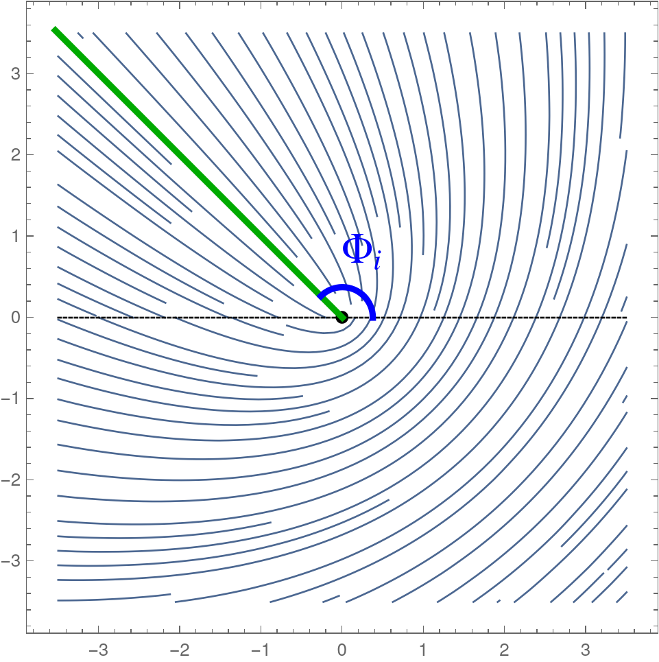
(a) $+1/2$

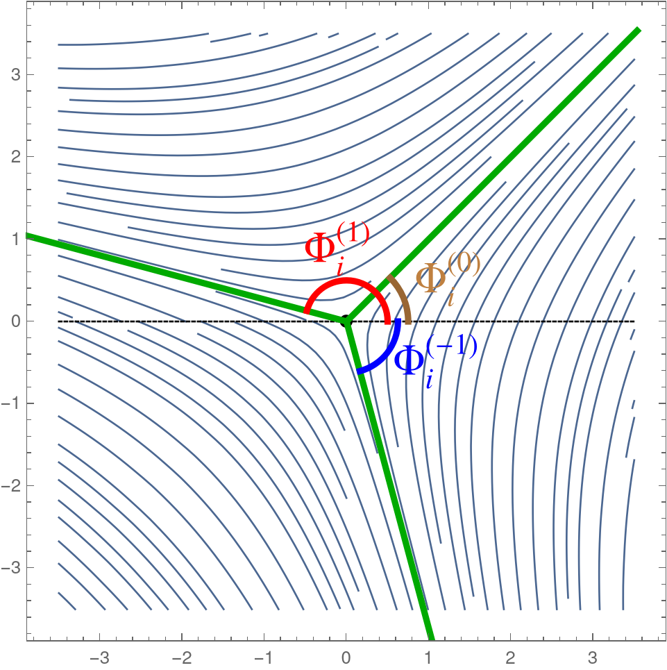
(b) $-1/2$ defect

Figure 1: Sketches of single defect textures showing the angles $\Phi_{i}$ for (a) a $+1/2$ defect where $\Phi_{i}=\phi_{i}=3\pi/4$, and (b) a $-1/2$ defect where $\Phi_{i}^{(k)}=\phi_{i}/3+2\pi k/3$ for $k=0\pm 1$.

Last but not least, we note that for a global rotation, under which $\varphi\rightarrow\varphi+\eta$ and $\psi\rightarrow\psi+\eta$, the complex order parameter transforms as $Q_{0}\to Q_{0}e^{i2\eta}$ , with the phase factor arising from the transformation of $\psi$. It follows that “defect phases” $\phi_{i}$ transform in a way that depends on the associated charge $\phi_{i}\to\phi_{i}+2(1-\sigma_{i})\eta$. In contrast, the phases $\Phi_{i}=\phi_{i}/(2-2\sigma_{i})$ transform naturally (i.e., shift by the rotation angle $\eta$) under rotation.

IV Derivation of the multi-defect dynamics equations

IV.1 Defect dynamics on the inertial manifold

Before considering active motion of defects, let us examine the relaxational dynamics on the inertial manifold governed by Eq. (7) with $\alpha=0$. Since we have the approximate solution $Q_{0}(z,{\bar{z}}|\{z_{i},{\bar{z}}_{i}\})$ which defines the free energy ${\cal F}_{0}(\{z_{i},{\bar{z}}_{i}\})\equiv{\cal F}(Q_{0})$ as a function of collective coordinates via Eq. (17), one expects ${\dot{z}}_{i}(t)={d\over dt}z_{i}$ to be determined by $\partial_{i}{\cal F}_{0}$. To simplify notation, we introduce a $2n$-dimensional (where $n$ is the number of defects) set of coordinates $\{\zeta_{k}\}=\{z_{i},{\bar{z}}_{i}\}$ (with $\zeta_{k}$ for $k=1,\ldots,n$ standing in for $z_{i}$ and $k=n+1,\ldots,2n$ denoting ${\bar{z}}_{i}$)

$${\dot{\zeta}}_{k}=-\sum_{l}m_{kl}{\bar{\partial}}_{l}{\cal F}_{0}\;.$$ (20)

Naively one may expect the mobility matrix to be diagonal, $m_{kl}=\delta_{kl}$, as would be the case if $z_{i}$ (and hence $\zeta_{k}$) were kinematically independent degrees of freedom, as often assumed Shankar et al. (2018). This is not, however, the case, as we will see by deriving defect dynamics on the inertial manifold $Q_{0}$ directly from Eq. (7). Restricting Eq. (7) to the $Q_{0}(z,{\bar{z}}|\{\zeta\})$ manifold gives

$$\partial_{t}Q(z,{\bar{z}}) =\sum_{k}{\dot{\zeta}}_{k}\partial_{k}Q_{0}(z,{\bar{z}}|\{\zeta\})=$$

$$=-\sum_{a}{\delta\zeta_{k}\over\delta{\bar{Q}}_{0}(z,{\bar{z}})}{\delta{\cal F}_{0}\over\delta\zeta_{k}}\;,$$ (21)

where we have formally used the chain rule of differentiation (and abbreviated $\partial_{k}=\partial_{\zeta_{k}}$) to evaluate $\delta{\cal F}_{0}/\delta Q_{0}$. The subtlety is in defining ${\delta\zeta_{k}\over\delta{\bar{Q}}_{0}(z)}$. While ${\delta{\bar{Q}}_{0}(z,\bar{z})\over\delta\zeta_{k}}=\partial_{k}{\bar{Q}}_{0}(z,\bar{z})$ is unambiguous, the meaning of the former is not obvious. To define it, we recall that the variation $\delta Q(z,\bar{z})$ is taken in the $L^{2}$ norm so that one can think of $\delta Q(z,\bar{z})$ as an $N$-dimensional vector (with $N\rightarrow\infty$) and of ${\delta{\bar{Q}}_{0}(z,\bar{z})\over\delta\zeta_{a}}$ as an $N\times 2n$ matrix. It is then natural to define ${\delta\zeta_{k}\over\delta{\bar{Q}}_{0}(z,\bar{z})}$ by the pseudo inverse so that it obeys

$$\delta_{kl} =\int dzd{\bar{z}}\left[{\delta\zeta_{k}\over\delta{\bar{Q}}_{0}(z,\bar{z})}{\delta{\bar{Q}}_{0}(z,\bar{z})\over\delta\zeta_{l}}+{\delta\zeta_{k}\over\delta{Q}_{0}(z,\bar{z})}{\delta{Q}_{0}(z,\bar{z})\over\delta\zeta_{l}}\right]$$

$$=2\int dzd{\bar{z}}{\delta\zeta_{k}\over\delta{\bar{Q}}_{0}(z,\bar{z})}{\delta{\bar{Q}}_{0}(z,\bar{z})\over\delta\zeta_{l}}\;,$$ (22)

where the second equality derives from the fact that to leading order $|Q_{0}|=1$ so that ${\bar{Q}}\delta Q=-Q\delta{\bar{Q}}$. This “completeness condition” is satisfied by

$${\delta\zeta_{k}\over\delta{\bar{Q}}_{0}(z,\bar{z})}={\bar{\partial}}_{l}{Q}_{0}(z,\bar{z})\mathcal{M}_{kl}^{-1}$$ (23)

(where we have adopted the Einstein repeated index summation convention) with a Hermitian matrix

$$\mathcal{M}_{kl}=2\int dzd{\bar{z}}\ \partial_{k}{\bar{Q}}_{0}{\bar{\partial}}_{l}{Q}_{0}\;.$$ (24)

The “overlap” matrix $\mathcal{M}_{kl}$ can be thought of as the intrinsic metric of the inertial manifold parameterized by collective coordinates $\{\zeta\}$. The explicit form of $\mathcal{M}_{kl}$ is computed in Appendix C.

Substituting into Eq. (21) we arrive at Eq. (20) and we identify

$$m_{kl}={\cal M}_{kl}^{-1}$$ (25)

relating the mobility matrix $m_{kl}$ to the metric ${\cal M}_{kl}$ of the inertial manifold.

IV.2 Defect dynamics in the presence of active stress.

To describe the nematic dynamics in the limit of weak activity and low defect density, we will assume that the order parameter texture $Q(z,{\bar{z}},t)$ stays close to the quasi-static manifold $Q_{0}(z,{\bar{z}}|\{z_{i}(t)\})$ parameterized by the time-dependent defect positions,

$$Q(z,{\bar{z}},t)=Q_{0}(z,{\bar{z}}|\{\zeta(t)\})+\epsilon^{2}\delta Q(z,{\bar{z}},t)$$ (26)

where the $\epsilon^{2}$ prefactor of $\delta Q$ provides correct scaling for the magnitude of the perturbation, as we shall see below. We rewrite the complex texture dynamics, Eq. (7), as

$${\dot{\zeta}}_{k}\partial_{k}Q_{0} +\epsilon^{2}\partial_{t}\delta Q=-{\delta{\cal F}\over\delta\bar{Q}}|_{(Q_{0}+\epsilon^{2}\delta Q)}+\alpha\mathcal{I}_{\alpha}(Q_{0}+\epsilon^{2}\delta Q)\;.$$ (27)

This serves as a starting point for our perturbation theory. Separating out variations within the inertial manifold described by the dynamics of $\{\zeta(t)\}$ from variations described by $\delta Q$ on the punctured plane, we have

$${\delta{\cal F}(\{Q\})\over\delta\bar{Q}}={\partial}_{k}{Q}_{0}\mathcal{M}_{kl}^{-1}{\delta{\cal F}_{0}\over\delta{\bar{\zeta}}_{l}}+\left[{\delta{\cal F}(\{Q\})\over\delta\bar{Q}}\right]_{\zeta}\;.$$ (28)

Substituting Eq. (28) into Eq. (27) and keeping terms to the linear order in activity and in $\epsilon^{2}$ leads to the linearized equation for $\delta Q$ in the form

$${\cal L}\delta Q+{\cal L}^{\prime} \delta{\bar{Q}}={\cal V}_{k}\partial_{k}Q_{0}-\alpha\mathcal{I}_{\alpha}(Q_{0})+{\cal O}(\epsilon^{2}\alpha,\epsilon^{2},\alpha^{2})\;,$$ (29)

with

$${\cal V}_{k}={\dot{\zeta}}_{k}+{\cal M}_{kl}^{-1}{\bar{\partial}}_{l}{\cal F}_{0}$$ (30)

representing the residual motion along the inertial manifold. We have also introduced the linear operators

$${\cal L}=2(1-2|Q_{0}|^{2})+4\epsilon^{2}\partial{\bar{\partial}}\;,$$ (31)

$${\cal L}^{\prime}=-2Q_{0}^{2}\;,$$ (32)

defined (on the punctured plane) by the linearization of ${\delta{\cal F}\over\delta Q(z)}(Q_{0}+\epsilon^{2}\delta Q)$. We note that $\epsilon^{2}\partial_{t}\delta Q$ does not appear in Eq. (29) to leading order in perturbation theory. In the limit of $\alpha\to 0$, $\delta Q\to 0+{\cal O}(\epsilon^{2})$ and ${\cal V}_{k}=0+{\cal O}(\epsilon^{2})$ which corresponds to the passive dynamics described by Eq. (20) with $m_{kl}={\cal M}_{kl}^{-1}$.

It is useful to reorganize Eq. (29) and its complex conjugate into a matrix form,

$$\left[\begin{matrix}&{\cal L}&{\cal L}^{\prime}\ \\ &{\bar{\cal L}}^{\prime}&{\cal L}\ \\ \end{matrix}\right]\left[\begin{matrix}&\delta Q\ \\ &\delta{\bar{Q}}\ \\ \end{matrix}\right]= {\cal V}_{k}\left[\begin{matrix}&\partial_{k}Q_{0}\ \\ &\partial_{k}{\bar{Q}}_{0}\ \\ \end{matrix}\right]-\alpha\left[\begin{matrix}\mathcal{I}_{\alpha}\ \\ \mathcal{\bar{I}}_{\alpha}\ \\ \end{matrix}\right]\;.$$ (33)

Crucially for our analysis, the linear operator on the left hand side of Eq. (33) has zero modes corresponding to infinitesimal changes of defect positions that enter $Q_{0}$ as free $\zeta_{k}$ parameters, or

$$\left[\begin{matrix}&{\cal L}&{\cal L}^{\prime}\ \\ &{\bar{\cal L}}^{\prime}&{\cal L}\ \\ \end{matrix}\right]\left[\begin{matrix}&\partial_{k}Q_{0}\ \\ &\partial_{k}{\bar{Q}}_{0}\ \\ \end{matrix}\right]=0\;,$$ (34)

as can be seen explicitly by differentiating ${\delta\mathcal{F}\over\delta Q}(Q_{0})=0$ (which holds within our approximation on the punctured plane) with respect to $\zeta_{k}$. This means that $\delta Q$ corrections must be orthogonal to the inertial manifold $Q_{0}(z,\bar{z}|\{\zeta\})$, something that was already anticipated in representing the dynamics of $Q$ in the form given in Eq. (26).

Hence the linear system of equations (33) for $\delta Q$ can only be solved if the inhomogeneous term is orthogonal to the null space of the linear operator, the so called “Fredholm alternative” condition Fredholm (1903). This solvability condition for Eq. (33) has the form

$$\mathcal{M}_{kl}{\cal V}_{l}=\alpha\int d^{2}z[\bar{\partial}_{k}\bar{Q}_{0}{\mathcal{I}}_{\alpha}+\bar{\partial}_{k}Q_{0}\bar{\mathcal{I}}_{\alpha}]\;,$$ (35)

with the same overlap matrix $\mathcal{M}_{kl}$ as appeared in the previous section and (see Appendix C)

$$\int dzd{\bar{z}}\ {\bar{\partial}}_{k}{\bar{Q}}_{0}{\partial}_{l}{Q}_{0}=\int dzd{\bar{z}}\ {\partial}_{k}{\bar{Q}}_{0}{\bar{\partial}}_{l}{Q}_{0}={1\over 2}\mathcal{M}_{kl}\;.$$ (36)

Substituting the definition of $\mathcal{V}_{k}$, we arrive at the system of ODEs governing the defect dynamics, given by

$$\mathcal{M}_{kl}{\dot{\zeta}}_{l}=-{\bar{\partial}}_{k}{\cal F}_{0}+\alpha\ {\cal U}_{k}\;,$$ (37)

with

$${\cal U}_{k}=\int dzd\bar{z}[\bar{\partial}_{k}\bar{Q}_{0}{\mathcal{I}}_{\alpha}+\bar{\partial}_{k}Q_{0}{\bar{\mathcal{I}}}_{\alpha}]\;.$$ (38)

Thus, flows driven by active stresses cause $Q$ to deviate from its form on the inertial manifold, with the deviation, $\delta Q$, limited by relaxational restoring forces. The component of active forcing that projects onto the tangent space of the inertial manifold shows up in the equations governing the dynamics of the defect positions $z_{i}(t)$. In the next section we will describe this dynamics more explicitly.

An alternative derivation of the defect dynamics (Eq. (37)) is given in Appendix E. We note also that the equations of motion for $z_{i}(t)$ obtained above minimize the deviation of the dynamics on the inertial manifold $Q_{0}$ from that described by the equation of motion, Eq. (7). In other words, the same dynamics can be obtained by minimizing

$$E =\int d^{2}dzd\bar{z}\left|\partial_{t}Q(z,{\bar{z}},t)-{d\over dt}Q_{0}(z,{\bar{z}}|\{z_{i}(t)\})\right|^{2}$$

$$\approx\int dzd\bar{z}\left|\mathcal{I}(Q_{0})-\dot{z}_{i}\partial_{i}Q_{0}-\dot{\bar{z}}_{i}\bar{\partial}_{i}Q_{0}\right|^{2}$$ (39)

with respect to $\dot{z}_{i}$, where $\mathcal{I}$ is defined in Eq. (7).

V Dynamics of defects in active nematics

In the previous section, we derived multi-defect dynamics based on a perturbation theory in defect density and activity. In this section, we present the explicit form of the resulting equations of motion, using the results for $\mathcal{M}_{kl}$ from Appendix C and for $\mathcal{U}_{k}$ from Appendix D, and discuss the nature of the various terms. For clarity, we return to the original notation where we denote with $z_{i}$ and $\bar{z}_{i}$ the defect coordinates.

V.1 Mobility matrix

The matrix ${\mathcal{M}}_{k\ell}$ on the left hand side of Eq. (37) is the inverse mobility matrix  Brady and Bossis (1988) representing the correlation in the motion of defects due to the non-orthogonality of the associated textures of order parameter. A nonlocal mobility is known to occur for colloidal particles in flow due to hydrodynamic interactions Brady and Bossis (1988). Evaluating Eq. (24) in Appendix C, we find that the $2n\times 2n$ matrix $\mathcal{M}_{k\ell}$ can be decomposed into four $n\times n$ blocks, and that the two off-diagonal blocks are much smaller than the diagonal parts, and hence we ignore it in the following. The two diagonal parts, which we denote by the $n\times n$ matrix $\mathcal{M}_{ij}$, are equal and given by

$$\mathcal{M}_{ij} \approx 4\pi\sigma_{i}\sigma_{j}\ln\frac{L}{r_{ij}}\;,$$ (40)

where

$$r_{ij}=\begin{cases}|z_{i}-z_{j}|\ &i\neq j\\ a\approx 0.8\epsilon\ &i=j\end{cases}$$ (41)

and $L$ is system size. Only the diagonal part of $\mathcal{M}_{ij}$ receives contributions from the defect cores.

V.2 Interactions due to active flows

We next present the result of evaluating the active forcing term $\mathcal{U}_{i}$ defined in Eq. (38). In Appendix D, we show that

$$\alpha{\cal U}_{i}= \quad\pi\alpha a^{-1}e^{i\phi_{i}}\delta_{2\sigma_{i},1}\ +\sum_{j\neq i}f_{ij}\;,$$ (42)

where

$$f_{ij}=-2\pi\alpha\frac{\sigma_{i}\sigma_{j}}{1-\sigma_{j}}{\bar{q}_{ij}-(-1)^{\delta_{\sigma_{i}+\sigma_{j},1}}q_{ij}\over{\bar{z}}_{i}-{\bar{z}}_{j}}$$ (43)

and

$$q_{ij}=e^{i\phi_{i}}\left(\frac{z_{i}-z_{j}}{\bar{z}_{i}-\bar{z}_{j}}\right)^{\sigma_{i}-1}=e^{2i(1-\sigma_{i})\Phi_{i}}\left(\frac{z_{i}-z_{j}}{\bar{z}_{i}-\bar{z}_{j}}\right)^{\sigma_{i}-1}\;,$$ (44)

with $\Phi_{i}=\frac{\phi_{i}}{2(1-\sigma_{i})}$ the defect phase defined in Fig. 3.

The first term in Eq. (42) is the well-known “self-propulsion” of the $\sigma_{i}=+1/2$ defect that arises from the flows that the defect itself generates  Giomi et al. (2013); Pismen (2013), with the phase factor $e^{i\phi_{i}}$ controlling the direction. The latter is therefore recognized as the polarization (unit) vector of the $+1/2$ defect (see for e.g. Vromans and Giomi (2016); Tang and Selinger (2017); Shankar et al. (2018)).

The second term describes forces induced by interaction with other defects, represented by the sum of pairwise terms, that like 2D Coulomb forces are inversely proportional to the pair separation $|z_{i}-z_{j}|$.

Unlike Coulomb forces, pairwise forces here are in general non-reciprocal and depend on the relative positions of all other defects through the phase factor $e^{i\phi_{i}}$, thus incorporating many-body effects. Note that $\bar{q}_{ij}-(-1)^{\delta_{\sigma_{i}+\sigma_{j},1}}q_{ij}$ is real, corresponding to a central force, only in the case of $\sigma_{i}=\sigma_{j}=1/2$. In all other cases, this factor is purely imaginary, corresponding to active forces that act normal to the line joining defect positions, thus resulting in a torque acting on the pair, that depends on the orientation of the pair relative to other defects and the order parameter in the far field.

Finally, for completeness we provide an explicit form of the multi-defect dynamics equations including both passive and active forces. After eliminating common factor of $4\pi$ from both sides, these are given by

$$\sum_{k}\left(\sigma_{i}\sigma_{k}\log\frac{L}{r_{ik}}\right)\dot{z}_{k}=2\sum_{j\neq i}\frac{\sigma_{i}\sigma_{j}}{{\bar{z}}_{i}-{\bar{z}}_{j}}+{\alpha e^{i\phi_{i}}\over 4a}\delta_{2\sigma_{i},1}$$

$$\quad-\frac{\alpha}{2}\sum_{j\neq i}\frac{\sigma_{i}\sigma_{j}}{(1-\sigma_{j})}{\bar{q}_{ij}-(-1)^{\delta_{\sigma_{i}+\sigma_{j},1}}q_{ij}\over{\bar{z}}_{i}-{\bar{z}}_{j}}\;.$$ (45)

The three terms on the right hand side are, in order, the Coulomb interaction, the active self-propulsion of the $+1/2$ defects, and the active interactions. This description of defect dynamics has a number of new features discussed below.

V.3 Non-centrality and non-reciprocity in active interactions

In contrast to Coulombic interaction between defects, interactions mediated by active flow cannot be described by additive pair potentials. Nevertheless, active force acting on a given defect is represented as a sum of of pairwise terms which one interprets as a force exerted by one defect on another, even though this force depends in a specific way (through tensor $q_{ij}$ appearing in Eq. (45)) on the global texture and hence on position of all other defects.

The active pairwise force term in Eq. (45) has a non-trivial form and we now examine it in greater detail. For a plus/minus disclination pair, we find that the force exerted on defect $i$ by defect $j$ is:

$$f_{ij}=-{i\pi\alpha\over 1-\sigma_{j}}{\sin[2(1-\sigma_{i})(\Phi_{i}-\theta_{ij})]\over{\bar{z}}_{i}-{\bar{z}}_{j}}\ \ \ \text{for}\ \ \sigma_{i}\neq\sigma_{j}\;,$$ (46)

where $\theta_{ij}$ is the angle of the line joining $z_{j}$ to $z_{i}$ relative to the $x$-axis and we have used $\phi_{i}=2(1-\sigma_{i})\Phi_{i}\,(\mod 2\pi)$. Notice that here, and in the following expressions, $\Phi_{i}-\theta_{ij}$ is the relative angle between the polarization and line connecting the defects. This force acts perpendicular to the line connecting the defects and is clearly non-reciprocal since $\sigma_{i}\neq\sigma_{j}$, hence $|f_{ij}|\neq|f_{ji}|$. As a result, the disclination pair will experience a net force acting on its center of mass, as well as a torque which tends to rotate the pair until the line joining the defect centers aligns with the far-field phase. This is particularly clear in a system with just a single neutral disclination pair. In this case, $2(1-\sigma_{i})\Phi_{i}=2\sigma_{j}\theta_{ij}+2\psi$. Hence $\sin[2(1-\sigma_{i})(\Phi_{i}-\theta_{ij})]=\sin(2\psi-2\theta_{ij})$. Assigning $\sigma_{i}=1/2$, $\sigma_{j}=-1/2$ (and defining $z_{i}-z_{j}=r_{ij}e^{i\theta_{ij}}$) we have

$$f_{ij} =-\frac{1}{3}\leavevmode\nobreak\ \frac{2i\pi\alpha e^{i\theta_{ij}}}{r_{ij}}\sin 2(\psi-\theta_{ij})$$

$$f_{ji} =\frac{2i\pi\alpha e^{i\theta_{ij}}}{r_{ij}}\sin 2(\psi-\theta_{ij})\;.$$ (47)

Due to the $1/(1-\sigma_{j})$ prefactor in Eq. (46), the force acting on the plus-disclination $(i)$ is 3 times smaller than the force acting on the minus-disclination $(j)$, resulting in a net force acting on the center of mass, perpendicular to the axis of the pair. There is also a torque $T_{ij}={2\over 3}|f_{ji}|r_{ij}$ that rotates the pair so as to align $\theta_{ij}$ with $\psi$ - the order parameter orientation in the far field. Physically, this dynamics is due to the entrainment of the defects to the active flows generated by the global texture, with rotational invariance broken by the nematic orientation in the far field.

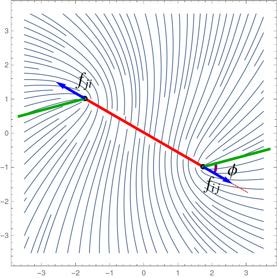
(a) $+1/2$ and $+1/2$ defects

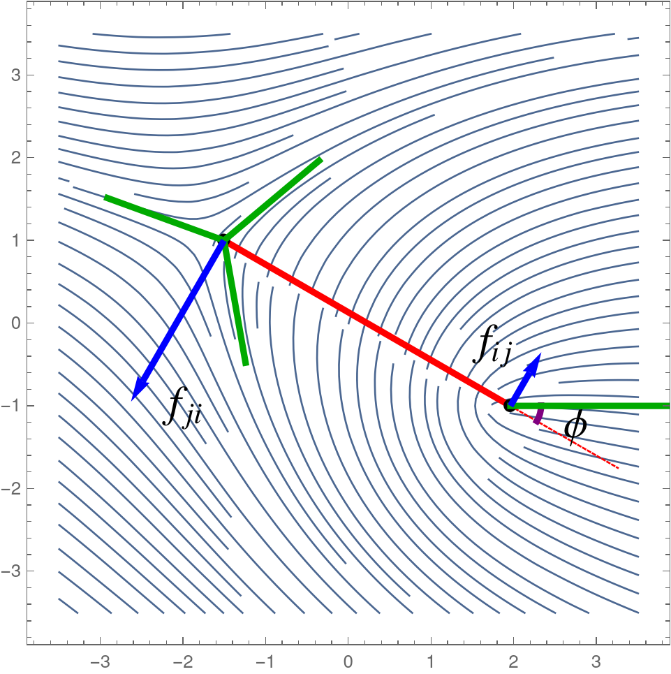
(b) $-1/2$ and $+1/2$ defects

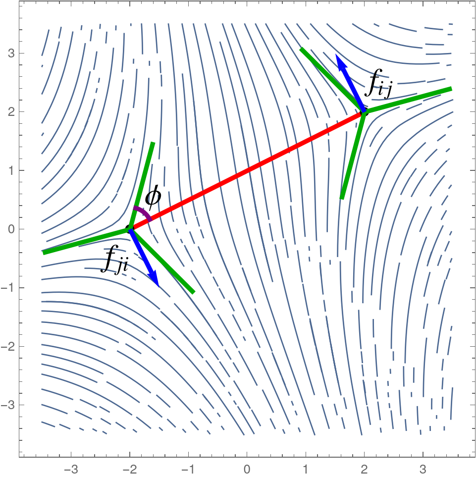
(c) $-1/2$ and $-1/2$ defects

Figure 2: Sketches of the active forces between defect pairs in an extensile system ($\alpha<0$). The blue arrows denote the forces, the red line joins the center of the two defects, and $\phi=\Phi_{i}-\theta_{ij}$ denotes the angle of the polarization relative to the line connecting the two defects. For $(+1/2,+1/2)$ pairs, the forces are radial, but for the $(-1/2,+1/2)$ and $(-1/2,-1/2)$ pairs, they are perpendicular to the line connecting the defects, generating rotations of the pair.

The force on a plus disclination at $z_{i}$ arising from a second plus disclination at $z_{j}$ is

$$f_{ij}={2\pi\alpha\cos(\Phi_{i}-\theta_{ij})\over{\bar{z}}_{i}-{\bar{z}}_{j}}\ \ \ \text{for}\sigma_{i}=\sigma_{j}=1/2\;.$$ (48)

This force acts along the line connecting the two defects. For a pair of plus-disclinations far away from all other defects, $\phi_{i}=\phi_{j}+\pi$, and so $f_{ij}+f_{ji}=0$. Otherwise, $\phi_{i}\neq\phi_{j}+\pi$, and so $f_{ij}+f_{ji}\neq 0$. This lack of reciprocity is due to the gradient of the “phase field” of the nematic texture. The presence of other defects cannot be forgotten in this case because a pair of same sign defects alone does not satisfy the boundary conditions at infinity: at least two negative charge disclinations must be present to satisfy (topological) charge neutrality. We also note explicit dependence of $f_{ij}$ on the phase of $Q$ at infinity, $2\psi$, (which additively contributes to $\phi_{i}$). Rotating this phase would modulate the magnitude of $f_{ij}$ - an effect that is made plausible by noting that the same phase uniformly rotates the active stress tensor everywhere and hence rotates the direction of active flow relative to $z_{i}-z_{j}$.

Finally, for a pair of minus-disclinations the force acting on $z_{i}$ is given by

$$f_{ij}={i2\alpha\pi\over 3}{\sin(3(\Phi_{i}-\theta_{ij}))\over{\bar{z}}_{i}-{\bar{z}}_{j}}\ \ \ \text{for}\ \ \sigma_{i}=\sigma_{j}=-{1\over 2}\;.$$ (49)

Like the force in a neutral pair, this force also acts perpendicular to the line $z_{i}-z_{j}$, thus generating a “2-body torque”. It is also non-reciprocal, thus yielding a net force acting on the pair.

The nonreciprocity and non-central character of the forces between defect pairs arise because the texture, as described by the $Q$ tensor, is nonlinear in the director, hence in the defect phases. So, even if we write the texture as a linear superposition of individual defect phases, the flow generated by the texture is a nonlinear superposition of the flow generated by individual defects. As a result, the flow near one defect depends on the flow due to the other defects, and this results in the form of the forces and torques.

V.4 Dynamics of $+1/2$ defect polarization

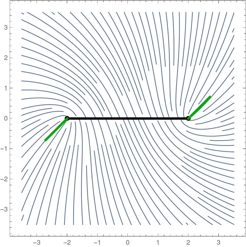
(a) Two neighboring $+1/2$ defects

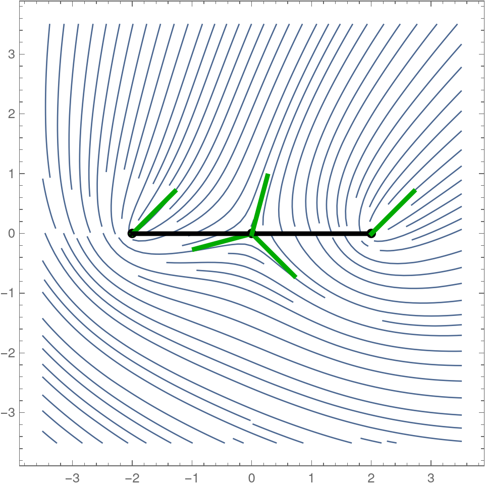
(b) Two $+1/2$ defects separated by a $-1/2$ defect

Figure 3: In (a), two neighboring $+1/2$ defects anti-align, and in (b), since the $+1/2$ defects are separated by a $-1/2$ defect, they align.

To illustrate our results and make contact with earlier work Keber et al. (2014); Shankar et al. (2018); Shankar and Marchetti (2019), we also construct an explicit equation for the dynamics of the polarization of a “tagged” $+1/2$ defect defined by the phase $\phi_{i}$ in the field of other defects. Differentiating Eq. (19) with respect to time, we obtain

$$\frac{d\phi_{i}}{dt}=-i\sum_{j\neq i}\sigma_{j}\left(\frac{\dot{z}_{i}-\dot{z}_{j}}{z_{i}-z_{j}}-c.c\right)\;.$$ (50)

For simplicity, we evaluate this equation in the dilute limit, when interaction between defects (and the off-diagonal elements of the mobility matrix) can be neglected and defect motion is dominated by the active drift of plus-defects, with the result

$$\frac{d\phi_{i}}{dt} \approx-ic\alpha\sum_{j\neq i}\frac{\sigma_{j}e^{i\phi_{i}}}{z_{i}-z_{j}}+ic\alpha\sum_{j^{+}\neq i}\frac{\sigma_{j_{+}}e^{i\phi_{j}}}{z_{i}-z_{j_{+}}}+c.c$$

$$=-2c\alpha\ {\cal E}_{i}\sin(\Theta_{i}-\phi_{i})-2c\alpha\sum_{j_{+}\neq i}{\sigma_{j_{+}}\over r_{ij_{+}}}\sin(\theta_{ij_{+}}-\phi_{j_{+}})\;,$$ (51)

where $c=[a\ln L/a]^{-1}$. In the 1st term, we have defined

$${\cal E}_{i}e^{i\Theta_{i}}=\sum_{j\neq i}{\sigma_{j}\over{\bar{z}}_{i}-{\bar{z}}_{j}}\;.$$ (52)

and in the 2nd term, the sum over ${j_{+}}$ runs only over plus-defects. Up to a numerical factor, ${\cal E}_{i}$ is the “electrostatic field” at point $z_{i}$ due to other defects. The 1st term in Eq. (51) describes the tendency of the plus-defect polarization in extensile (contractile) systems to align (anti-align) with the direction of net Coulomb force acting on it. This term already appeared in the equation for polarization dynamics derived in Shankar et al. (2018) by examining the dynamics of a single defect in the mean field of other defects. It is purely kinematic in origin as it arises from defect self-advection. The second term in Eq. (51) is new. The general structure of the polarization dynamics equation persists when defect dynamics ${\dot{z}}_{i}$ includes interaction terms of Eq. (45), which will cause the motion of minus-defects contributing to the second term in Eq. (51). Finally, we note in our formulation of the problem the equation for defect polarization dynamics is superfluous, as this polarization is defined kinematically by defect positions via Eq. (19).

Explicit dependence of polarization on defect positions given by Eq. (19) provides some useful insights. For example, it is easy to see that two neighboring plus disclinations far removed from all other defects have their polarizations anti-align with each other (independent of the orientation of the pair axis). However, the presence of a minus-disclination (or plus-disclination) in between leads to the alignment of the polarizations of the two flanking plus-disclinations (see Fig. 3). These effects have been noted in earlier work on defect orientation Vromans and Giomi (2016); Tang and Selinger (2017), as well as in recent numerical and experimental studies Pearce et al. (2020); Thijssen et al. (2020).

VI Discussion

We have presented a general formalism, based on perturbation theory in activity and defect density, to derive a set of coupled ordinary differential equations governing multi-defect dynamics for a 2D active nematic deep in the nematic phase. Our analysis goes beyond earlier work that obtained the dynamics of a single “tagged” defect in the mean-field of other defects Shankar et al. (2018), to capture the coupled dynamics of a many-defect texture. This yields a number of new results and explicitly demonstrates the non-central and non-reciprocal nature of active stress-induced defect-defect interactions Maitra et al. (2020).

Central to our approach is the realization that deep in the nematic state, order parameter textures stay close to a 2N-dimensional “inertial manifold” defined by the quasi-static multi-defect solution $Q_{0}$ parameterized by defect positions. By explicitly describing multi-defect configurations, we obtain a closed formulation that describes defect dynamics entirely in terms of the defect positions. This avoids the need to treat polarization as an independent degree of freedom, as was done in the earlier work by some of us Shankar et al. (2018). Here the polarization of the $+1/2$ defect and the orientation of the $-1/2$ as defined by the “defect phase” $\Phi_{i}$ are expressed explicitly in terms of defect positions through Eq. (19). Dynamics of the latter defines the relatively slow flow on the inertial manifold of textures by comparison to the rapid ($\sim{\cal O}(\epsilon^{-2})$) rate of relaxation of deviations away from the manifold. This separation of time-scales enables the perturbation theory about the $Q_{0}$ manifold.

The separation of time scales that enables us to describe the dynamics of $Q$ by projecting it onto the inertial manifold holds as long as the mean separation between defects is large compared to the coherence length $\xi$ ($\epsilon^{2}\ll 1$). In our analysis here, the defect density was treated as given by the initial condition. More realistically, nematic disclinations are subject to pairwise creation and annihilation. Extensive simulations of the continuum equations of active nematics have demonstrated that the state of spatio-temporal chaotic defect dynamics is characterized by a steady mean defect density $\ell^{-2}=\ell_{active}^{-2}\sim\alpha$ Giomi (2015); Hemingway et al. (2016); Doostmohammadi et al. (2018). For weak activity, this regime falls within the range of validity of our perturbation theory, even though we introduced it as an independent double expansion in $\epsilon^{2},\alpha\ll 1$.

One of the new results of our analysis is the recognition that defect velocities are directly coupled to each other through the inverse mobility matrix (on the left hand side of Eq. (45)). This effect, while resembling a “collective drag”, is purely kinematic in origin as it arises from the non-orthogonality of order parameter deformations, $\partial_{i}Q_{0}$, associated with translational motion of individual defects. The overlap of these modes defines the metric of the inertial manifold parameterized by defect positions. Off-diagonal elements of the mobility matrix are only logarithmically smaller than the diagonal ones $\sim\log(L/r_{ij})/\log(L/a)$.

Typical of 2D physics with soft modes, the mobility depends logarithmically on the size of the system $L$. Our formal way of dealing with the underlying infrared divergence has been to assume that defects are confined to a region much smaller than the size of the system $L$. It would however be straightforward to carry out the analysis in a finite disc, which can be done using the method of images as outlined in Appendix F. Alternatively, our analysis can be carried out on the surface of a sphere or of a torus, where IR modes would be naturally cutoff by the radius. We note that the study of such geometries is directly relevant to experiments that have realized active nematics on such curved surfaces Keber et al. (2014); Ellis et al. (2018).

We note that non-diagonal mobility enters already in the purely relaxation dynamics of defects driven by Coulomb interactions in the passive nematic. Although the Coulomb interaction is reciprocal, so that the total force on the system of defects is exactly zero, the center of mass (COM) $\sum_{i}z_{i}$ can nevertheless move, provided that there are more than two defects (as can be seen directly from Eq. (45)). This result may be counter intuitive, but it means simply that under relaxational dynamics, the defect system never translates rigidly as a whole and the motion of the COM is always accompanied by a change in defect configuration. By adding active forces with a suitable time dependence, it may be possible to take the system through a cycle that at the end restores relative position of the defects, but the possibility of a shift of the COM generated by such a “stroke” would not be a surprise.

Our analysis can be easily extended to include the interaction of defects with elastic deformations of the nematic order. To do that, one needs to replace the fixed phase $\psi$ in our definition of the $Q_{0}$ texture with an arbitrary harmonic function: $\Psi(z,t)+c.c$. With this generalization, $Q_{0}$ would still minimize ${\cal F}$ on the punctured plane. $\Psi(z,t)$ allows to represent the effect of the external forcing acting and to compute finite size corrections as shown in Appendix F.

Our work provides a unified framework for describing the dynamics of defects in active nematics and investigating the possibility of dynamical phases of defect order. Conflicting results have been reported in experiments and simulations with both polar and apolar (antiferromagnetic) order of the polar $+1/2$ defects reported by different authors  DeCamp et al. (2015); Putzig et al. (2016); Oza and Dunkel (2016); Srivastava et al. (2016); Ellis et al. (2018); Shankar et al. (2018); Pearce et al. (2020); Thijssen et al. (2020). While there have been suggestions that the type and range of defect order may be affected by the importance of density fluctuations and viscous dissipation, which are not included in the present calculation, the defects ODEs derived here could be used to settle some of these open questions. It would also be interesting to investigate the possibility of ordered lattices of defects accompanied by a regular array of flow vortices and resembling Abrikosov lattices in type-II superconductors that has been reported in simulations Doostmohammadi et al. (2016b).

While this manuscript was being prepared, we learned of the preprint by Y-H. Zhang, M. Deserno and Z-C. Tu posted on the arXiv Zhang et al. (2020). In this work, Zhang et al. derive - by a variational method similar to our Eq. (39) - active nematic defect dynamics equations for 4 plus disclinations on a sphere.

Appendices

Appendix A Defect core structure

Stationary textures in the limit of zero activity ($\alpha=0$) minimize LdG free energy and hence solve  De Gennes and Prost (1993); Pismen (1999)

$${\delta{\cal F}\over\delta{\bar{Q}}}=-\nabla^{2}Q-2\epsilon^{-2}(1-|Q|^{2})Q=0\;,$$ (53)

the imaginary and the real part of which read, respectively,

$$\nabla^{2}\theta+2\nabla\log A\cdot\nabla\theta=0$$ (54)

and

$$(1-A^{2})={\epsilon^{2}\over 2}\left[A^{-1}\nabla^{2}A-(\nabla\theta)^{2}\right]\;.$$ (55)

We look for a solution for a single defect of charge $\sigma$ of the form

$$Q=A(r)e^{2i\sigma\varphi}\;.$$ (56)

$A(r)$ would thus satisfy

$$A^{\prime\prime}(r)+\frac{A^{\prime}}{r}+\left(2\epsilon^{-2}-\frac{\sigma^{2}}{r^{2}}-2\epsilon^{-2}A^{2}\right)A=0\;.$$ (57)

For example, for $\sigma=\pm 1/2$, $A(r)$ can be approximated as Pismen (1999)

$$A(r)=\tilde{r}\sqrt{\frac{.68+.28\tilde{r}^{2}}{1+.82\tilde{r}^{2}+.28\tilde{r}^{4}}}\;,$$ (58)

where $\tilde{r}=r/\epsilon$. As $r\to 0$, $A(r)\propto r$, and for $r\gg\epsilon$, $A(r)\simeq 1-\frac{\epsilon^{2}}{4r^{2}}$. The defect core size $a$, which is the length scale over which $A$ goes from 0 to 1, is of the order $a\sim\epsilon$. As we will see later in the appendices, it is convenient for us to define the core size to be $a\approx 0.8\epsilon$.

Appendix B Free energy of the multi-defect texture

Here we compute the free energy in the passive case. For our ansatz $Q_{0}$, we have

$$\mathcal{F}(Q_{0}) =4\int d^{2}z|\partial\theta|^{2}=4\int d^{2}z\sum_{ij}\frac{\sigma_{i}\sigma_{j}}{(\bar{z}-\bar{z}_{i})(z-z_{j})}$$

$$={\color[rgb]{0,0,0}-8\pi\sum_{i\not=j}\sigma_{i}\sigma_{j}\ln\frac{|z_{i}-z_{j}|}{L}+C}\;,$$ (59)

where $C$ is a constant that accounts for the sum of the core energy of all defects Chaikin and Lubensky (2000). So in the passive case we can view the free energy $\mathcal{F}$ as a function of defect positions $z_{i}$.

Appendix C Computation of $\mathcal{M}_{ab}$

In this appendix, we compute the metric tensor of the multi-defect manifold $\mathcal{M}_{k\ell}$ by computing the “overlaps”. We can express the $2n\times 2n$ matrix $M_{k\ell}$ as a block matrix of four $n\times n$ matrices:

$$\mathcal{M}_{k\ell}=\begin{pmatrix}\mathcal{M}_{ij}&\mathcal{N}^{\dagger}_{ij}\\ \mathcal{N}_{ij}&\mathcal{M}_{ij}\end{pmatrix}\;,$$ (60)

where

$$\mathcal{M}_{ij}=2\int d^{2}z\partial_{i}\bar{Q}_{0}\bar{\partial}_{j}Q_{0}$$ (61)

$$\mathcal{N}_{ij}=2\int d^{2}z\bar{\partial}_{i}\bar{Q}_{0}\bar{\partial}_{j}Q_{0}\;.$$ (62)

Using the integrals below, it is easy to see that $M_{ij}$ and $\mathcal{N}_{ij}$ are both symmetric, and moreover, $\mathcal{M}_{ij}$ is real.

In the deep nematic limit, we can take $A=1$:

$${\cal M}_{ij}=\int d^{2}z{\sigma_{j}\over{\bar{z}}-{\bar{z}}_{j}}{\sigma_{i}\over z-z_{i}}$$

$$=2\int dzd{\bar{z}}{\sigma_{i}\sigma_{j}\over{\bar{z}}[z-(z_{j}-z_{i})]}$$

$$=2\sigma_{i}\sigma_{j}\int_{a}^{L}{dR\over R}\oint\limits_{R}{dz\over i[z-(z_{j}-z_{i})]}$$

$$=4\pi\sigma_{i}\sigma_{j}\int_{|z_{j}-z_{i}|}^{L}{dR\over R}$$ (63)

so that

$${\cal M}_{ij}=4\pi\sigma_{i}\sigma_{j}\log{L\over\max(|z_{j}-z_{i}|,a)}\;.$$ (64)

Here $a=0.8\epsilon$, as we will see below in a more careful treatment, by accounting for the fact that near the defect core $A\neq 1$.

We can also calculate $\mathcal{N}_{ij}$, which is given by

$$\mathcal{N}_{ij}=-2\int d^{2}z\frac{\sigma_{i}\sigma_{j}}{(\bar{z}-\bar{z}_{i})(\bar{z}-\bar{z}_{j})}\;.$$ (65)

We first note that for $i=j$, $\mathcal{N}_{ii}$ vanishes due to the phase integral. Thus below we assume $i\neq j$.

Shifting $z\to z+z_{j}$ and then rescaling $z\to z_{ij}z$, we have

$$\mathcal{N}_{ij}=-2\int d^{2}z\frac{\sigma_{i}}{\bar{z}-\bar{z}_{ij}}\frac{\sigma_{j}}{\bar{z}}=2\sigma_{i}\sigma_{j}\frac{z_{ij}}{\bar{z}_{ij}}\int\frac{dzd{\bar{z}}}{{\bar{z}}(1-{\bar{z}})}\;.$$ (66)

Splitting the region of integration to $|z|<1$, and $|z|>1$, and analytically expanding the integrand near $z=0$ (for $|z|<1$) and $z=\infty$ (for $|z|>1$) yields

$$\mathcal{N}_{ij}=2\pi\sigma_{i}\sigma_{j}\frac{z_{ij}}{\bar{z}_{ij}}\;.$$ (67)

Since we’re interested in the large $L$ limit, $|\mathcal{M}_{ij}|\gg|\mathcal{N}_{ij}|$, and thus in this paper we will ignore $\mathcal{N}_{ij}$ and set $\mathcal{N}_{ij}=0$.

C.1 A more careful treatment of the core for $\mathcal{M}_{ii}$

In order to compute $\mathcal{M}_{ii}$, we need to take into account the fact that near defect cores, $A\neq 1$ Pismen (1999); Chaikin and Lubensky (2000). We have

$$\mathcal{M}_{ii} =\int d^{2}zA^{2}\left(-\bar{\partial}\ln A_{i}-\frac{\sigma_{i}}{\bar{z}-\bar{z}_{i}}\right)\left(-\partial\ln A_{i}-\frac{\sigma_{i}}{z-z_{i}}\right)$$

$${}\,+\int d^{2}zA^{2}\left(-\bar{\partial}\ln A_{i}+\frac{\sigma_{i}}{\bar{z}-\bar{z}_{i}}\right)\left(-\partial\ln A_{i}+\frac{\sigma_{i}}{z-z_{i}}\right)$$

$$=2\int d^{2}zA^{2}\left[|\partial\ln A_{i}|^{2}+\frac{\sigma_{i}^{2}}{|z-z_{i}|^{2}}\right]$$

$$=\int d^{2}z\frac{1}{2}(A^{\prime})^{2}+2\sigma_{i}^{2}\int d^{2}z\frac{A^{2}}{|z-z_{i}|^{2}}$$

$$=4\pi\sigma_{i}^{2}\ln\frac{L}{a}\;,$$ (68)

where $a\approx 0.8\epsilon$ (using the approximate solution for $A$ in Eq. (58)).

Appendix D Computation of $U_{i}$

We are interested in computing

$$U_{i}=\int d^{2}z\bar{\partial}_{i}\bar{Q}\mathcal{I}_{\alpha}+\int d^{2}z\bar{\partial}_{i}Q\bar{\mathcal{I}}_{\alpha}=I_{1}+I_{2}\;,$$ (69)

where

$$I_{1} =\int d^{2}z\bar{\partial}_{i}\bar{Q}[Q\partial^{2}Q-(\partial Q)^{2}]-\int d^{2}z\bar{\partial}_{i}Q[\bar{Q}\partial^{2}Q+\partial Q\partial\bar{Q}]$$ (70)

$$I_{2} =\int d^{2}z\bar{\partial}_{i}Q[\bar{Q}\bar{\partial}^{2}\bar{Q}-(\bar{\partial}\bar{Q})^{2}]-\int d^{2}z\bar{\partial}_{i}\bar{Q}[Q\bar{\partial}^{2}\bar{Q}+\bar{\partial}\bar{Q}\bar{\partial}Q]\;.$$ (71)

We compute $I_{1}$ and $I_{2}$ in order.

D.1 Computation of $I_{1}$

Here we assume that $A=1$, as is the case in the deep nematic limit. A more careful treatment can be found later in this appendix.

We first note that

$$Q_{0}\partial^{2}Q_{0}-(\partial Q_{0})^{2} =-Q_{0}^{2}\sum_{j}\frac{\sigma_{j}}{(z-z_{j})^{2}}$$ (72)

$$\bar{Q}_{0}\partial^{2}Q_{0}+\partial Q_{0}\partial\bar{Q}_{0} =-\sum_{j}\frac{\sigma_{j}}{(z-z_{j})^{2}}\;.$$ (73)

Then

$$\bar{\partial}_{i}\bar{Q}_{0}(Q_{0}\partial^{2}Q_{0}-(\partial Q_{0})^{2})-\bar{\partial}_{i}Q_{0}(\bar{Q}_{0}\partial^{2}Q_{0}+\partial Q_{0}\partial\bar{Q}_{0})=$$

$$2Q_{0}\frac{\sigma_{i}}{\bar{z}-\bar{z}_{i}}\sum_{j}\frac{\sigma_{j}}{(z-z_{j})^{2}}\;.$$ (74)

Therefore,

$$I_{1}\approx 2\int d^{2}zQ_{0}\frac{\sigma_{i}}{\bar{z}-\bar{z}_{i}}\sum_{j}\frac{\sigma_{j}}{(z-z_{j})^{2}}\;.$$ (75)

We can write

$$I_{1}=I_{\text{leading}}+I_{\text{sub}}\;,$$ (76)

where

$$I_{\text{leading}} =2\int d^{2}zQ_{0}\frac{\sigma_{i}^{2}}{|z-z_{i}|^{2}}\frac{1}{z-z_{i}}$$ (77)

$$I_{\text{sub}} =2\int d^{2}zQ_{0}\frac{\sigma_{i}}{\bar{z}-\bar{z}_{i}}\sum_{j\neq i}\frac{\sigma_{j}}{(z-z_{j})^{2}}\;.$$ (78)

We explicitly compute and find that

$$I_{\text{leading}}=4\pi\sigma_{i}^{2}\alpha Q_{i}\delta_{2\sigma_{i},1}\int dr\frac{1}{r^{2}}=4\pi\sigma_{i}^{2}\frac{\alpha}{a}Q_{i}\delta_{2\sigma_{i},1}\;,$$ (79)

where

$$Q_{i}=\prod_{j\neq i}\frac{(z_{i}-z_{j})^{\sigma_{j}}}{(\bar{z}_{i}-\bar{z}_{j})^{\sigma_{j}}}\;.$$ (80)

We will see later in the subsection of this appendix that a more careful treatment again yields $a\approx 0.8\epsilon$.

We now compute the subleading term $I_{\text{sub}}$:

$$I_{\text{sub}}\approx\sigma_{i}\sigma_{j}Q_{ij}\int d^{2}z\frac{(z-z_{i})^{\sigma_{i}}}{(\bar{z}-\bar{z}_{i})^{\sigma_{i}}}\ \frac{(z-z_{j})^{\sigma_{j}}}{(\bar{z}-\bar{z}_{j})^{\sigma_{j}}}\frac{1}{\bar{z}-\bar{z}_{i}}\frac{1}{(z-z_{j})^{2}}\;,$$ (81)

where

$$Q_{ij}=\prod_{r\neq i,j}\frac{(z_{i}-z_{r})^{\sigma_{r}}}{(\bar{z}_{i}-\bar{z}_{r})^{\sigma_{r}}}\;.$$ (82)

Shifting $z\to z+z_{j}$, we have

$$I_{\text{sub}}\approx\sigma_{i}\sigma_{j}Q_{ij}\int d^{2}z\frac{(z-z_{ij})^{\sigma_{i}}}{(\bar{z}-\bar{z}_{ij})^{\sigma_{i}}}\ \frac{z^{\sigma_{j}}}{\bar{z}^{\sigma_{j}}}\frac{1}{\bar{z}-\bar{z}_{ij}}\frac{1}{z^{2}}\;.$$ (83)

Rescaling $z\to z_{ij}z$, we have

$$I_{\text{sub}}=\sigma_{i}\sigma_{j}q_{ij}\frac{I^{(1)}_{ij}}{\bar{z}_{ij}}\;,$$ (84)

where

$$q_{ij} =Q_{i}\hat{z}_{ij}^{2(\sigma_{i}-1)}$$ (85)

$$I^{(1)}_{ij} =\int d^{2}z\frac{(z-1)^{\sigma_{i}}}{(\bar{z}-1)^{\sigma_{i}}}\frac{z^{\sigma_{j}}}{\bar{z}^{\sigma_{j}}}\frac{1}{\bar{z}-1}\frac{1}{z^{2}}\;.$$ (86)

We’ll now outline how to compute $I^{(1)}_{ij}$. We first make the change of variables

$$w^{2}=\frac{z}{z-1}\;.$$ (87)

Then we split the region of integration to $|w|<1$, and $|w|>1$, and finally, we analytically expand the integrand near $w=0$ and $w=\infty$. Noting that $I^{(1)}_{ij}$ vanishes unless the powers of $w$ and $\bar{w}$ are equal yields

$$I^{(1)}_{ij} =(-1)^{\delta_{\sigma_{i}+\sigma_{j},1}}\frac{\pi}{1-\sigma_{j}}\;.$$ (88)

We want to remark that this expression is valid for $(\sigma_{i},\sigma_{j})=(\pm 1/2,\pm 1/2)$.

D.2 Computation of $I_{2}$

We first note that

$$Q_{0}\bar{\partial}^{2}\bar{Q}_{0}+\bar{\partial}\bar{Q}_{0}\bar{\partial}Q_{0} =-\sum_{j}\frac{\sigma_{j}}{(\bar{z}-\bar{z}_{j})^{2}}$$ (89)

$$\bar{Q}_{0}\bar{\partial}^{2}\bar{Q}_{0}-(\bar{\partial}\bar{Q}_{0})^{2} =-\bar{Q}_{0}^{2}\sum_{j}\frac{\sigma_{j}}{(\bar{z}-\bar{z}_{j})^{2}}\;.$$ (90)

Then

$$-\bar{\partial}_{i}\bar{Q}_{0}[Q_{0}\bar{\partial}^{2}\bar{Q}_{0}+\bar{\partial}\bar{Q}_{0}\bar{\partial}Q_{0}]+\bar{\partial}_{i}Q_{0}[\bar{Q}_{0}\bar{\partial}^{2}\bar{Q}_{0}-(\bar{\partial}\bar{Q}_{0})^{2}]=$$

$$-2\bar{Q}_{0}\frac{\sigma_{i}}{\bar{z}-\bar{z}_{i}}\sum_{j}\frac{\sigma_{j}}{(\bar{z}-\bar{z}_{j})^{2}}\;.$$ (91)

Therefore

$$I_{2} =-2\int d^{2}z\bar{Q}_{0}\frac{\sigma_{i}}{\bar{z}-\bar{z}_{i}}\sum_{j}\frac{\sigma_{j}}{(\bar{z}-\bar{z}_{j})^{2}}\;.$$ (92)

We now compute $I_{2}$:

$$I_{2} \approx-\sigma_{i}\sigma_{j}\bar{Q}_{ij}\int d^{2}z\frac{(\bar{z}-\bar{z}_{i})^{\sigma_{i}}}{(z-z_{i})^{\sigma_{i}}}\ \frac{(\bar{z}-\bar{z}_{j})^{\sigma_{j}}}{(z-z_{j})^{\sigma_{j}}}\frac{1}{\bar{z}-\bar{z}_{i}}\frac{1}{(\bar{z}-\bar{z}_{j})^{2}}\;.$$ (93)

Shifting $z\to z+z_{j}$, we have

$$I_{2}=-\sigma_{i}\sigma_{j}\bar{Q}_{ij}\int d^{2}z\frac{(\bar{z}-\bar{z}_{ij})^{\sigma_{i}}}{(z-z_{ij})^{\sigma_{i}}}\ \frac{\bar{z}^{\sigma_{j}}}{z^{\sigma_{j}}}\frac{1}{\bar{z}-\bar{z}_{ij}}\frac{1}{\bar{z}^{2}}\;.$$ (94)

Rescaling $z\to z_{ij}z$, we have

$$I_{2}=-\sigma_{i}\sigma_{j}\bar{q}_{ij}\frac{I^{(2)}_{ij}}{\bar{z}_{ij}}\;,$$ (95)

where

$$I^{(2)}_{ij}=\int d^{2}z\frac{(\bar{z}-1)^{\sigma_{i}}}{(z-1)^{\sigma_{i}}}\frac{\bar{z}^{\sigma_{j}}}{z^{\sigma_{j}}}\frac{1}{\bar{z}-1}\frac{1}{\bar{z}^{2}}\;.$$ (96)

To compute $I^{(2)}_{ij}$, we use the same method that we used to compute $I^{(1)}_{ij}$. Doing so yields

$$I^{(2)}_{ij} =\frac{\pi}{1-\sigma_{j}}\;.$$ (97)

Note that $|I^{(1)}_{ij}|=|I^{(2)}_{ij}|$, and the sign differs only when $\sigma_{i}+\sigma_{j}=1$.

D.3 A more careful treatment of the cores for $I_{\text{leading}}$

In order to quantify $a$ in the leading contribution, we need to take into account the deviation of $A$ away from 1 near the defect cores. Doing so yields

$$I_{\text{leading}} =2\int d^{2}zQ_{0}A^{2}\left[\frac{\sigma_{i}^{2}}{|z-z_{i}|^{2}}\frac{1}{z-z_{i}}-\frac{\sigma_{i}}{\bar{z}-\bar{z}_{i}}\partial^{2}\ln A_{i}\right.$$

$$\quad\left.+|\partial\ln A_{i}|^{2}\partial\ln A_{i}-\frac{\sigma_{i}}{\bar{z}-\bar{z}_{i}}(\partial\ln A_{i})^{2}\right.$$

$$\left.-\frac{\sigma_{i}^{2}}{|z-z_{i}|^{2}}\partial\ln A_{i}+|\partial\ln A_{i}|^{2}\frac{\sigma_{i}}{z-z_{i}}\right]\;.$$ (98)

We first compute $I_{\text{leading}}$ by computing each term separately:

$$-2\int d^{2}zQ_{0}A^{2}\frac{\sigma_{i}}{\bar{z}-\bar{z}_{i}}\partial^{2}\ln A_{i}$$

$$\qquad=-\pi\sigma_{i}\delta_{2\sigma_{i},1}Q_{i}\int drA\left[AA^{\prime\prime}-(A^{\prime})^{2}-\frac{AA^{\prime}}{r}\right]$$ (99)

$$2\int d^{2}zQ_{0}A^{2}\frac{\sigma_{i}^{2}}{|z-z_{i}|^{2}}\frac{1}{z-z_{i}}=4\pi\sigma_{i}^{2}\delta_{2\sigma_{i},1}Q_{i}\int dr\frac{A^{3}}{r^{2}}$$ (100)

$$2\int d^{2}zQ_{0}A^{2}|\partial\ln A_{i}|^{2}\partial\ln A_{i}=\frac{1}{2}\pi\delta_{2\sigma_{i},1}Q_{i}\int drr(A^{\prime})^{3}$$ (101)

$$-2\int d^{2}zQ_{0}A^{2}\frac{\sigma_{i}}{\bar{z}-\bar{z}_{i}}(\partial\ln A_{i})^{2}=-\pi\sigma_{i}\delta_{2\sigma_{i},1}Q_{i}\int drA(A^{\prime})^{2}$$ (102)

$$-2\int d^{2}zQ_{0}A^{2}\frac{\sigma_{i}^{2}}{|z-z_{i}|^{2}}\partial\ln A_{i}=-2\pi\sigma_{i}^{2}\delta_{2\sigma_{i},1}Q_{i}\int dr\frac{A^{2}A^{\prime}}{r}$$ (103)

$$2\int d^{2}zQ_{0}A^{2}|\partial\ln A_{i}|^{2}\frac{\sigma_{i}}{z-z_{i}}=\pi\sigma_{i}\delta_{2\sigma_{i},1}Q_{i}\int drA(A^{\prime})^{2}\;.$$ (104)

Combining all of these terms and computing, we find that

$$I_{\text{leading}}\approx$$

$$\quad 2\pi\sigma_{i}^{2}\alpha Q_{i}\delta_{2\sigma_{i},1}\int dr\left[-A^{2}A^{\prime\prime}+A(A^{\prime})^{2}+\frac{2A^{3}}{r^{2}}+r(A^{\prime})^{3}\right]$$

$$\quad\approx 4\pi\sigma_{i}^{2}\frac{\alpha}{a}Q_{i}\delta_{2\sigma_{i},1}\;,$$ (105)

where $a\approx 0.8\epsilon$ (using the approximate solution for $A$ in Eq. (58)).

Appendix E Alternative derivation of multi-defect dynamics equation

To describe nematic dynamics in the limit of weak activity and low defect density, we shall assume that the order parameter texture $Q(z,{\bar{z}},t)$ stays close to the inertial manifold $Q_{0}(z,{\bar{z}}|\{z_{i}(t)\})$ parameterized by time-dependent defect positions:

$$Q(z,{\bar{z}},t)=Q_{0}(z,{\bar{z}}|\{z_{i}(t)\})+\delta Q(z,{\bar{z}},t)\;,$$ (106)

where $\delta Q$ is locally perpendicular to the inertial manifold as defined by

$$\int dzd{\bar{z}}\ \partial_{i}\bar{Q}_{0}\delta Q=\int dzd{\bar{z}}\ {\bar{\partial}}_{i}\bar{Q}_{0}\delta Q=0\;.$$ (107)

We thus rewrite the complex texture dynamics equation Eq. (7) as

$${\dot{z}}_{i}\partial_{i}Q_{0}+{\dot{\bar{z}}}_{i}{\bar{\partial}}_{i}Q_{0} +\partial_{t}\delta Q=\mathcal{I}$$

$$=-{\delta{\cal F}(\{Q\})\over\delta\bar{Q}}+\alpha\mathcal{I}_{\alpha}(Q)\;.$$ (108)

Multiplying by $\partial_{i}\bar{Q}_{0}$ and integrating over space, we find that

$$\dot{z}_{j}\int dzd{\bar{z}}\partial_{i}\bar{Q}_{0}\partial_{j}Q_{0}+\dot{\bar{z}}_{j}\int dzd{\bar{z}}\partial_{i}\bar{Q}_{0}\bar{\partial}_{j}Q_{0}=\int dzd{\bar{z}}\partial_{i}\bar{Q}_{0}\mathcal{I}\;.$$ (109)

Similarly, if we multiply by $\bar{\partial}_{i}\bar{Q}_{0}$ and integrate over space, we find that

$$\dot{z}_{j}\int dzd{\bar{z}}\bar{\partial}_{i}\bar{Q}_{0}\partial_{j}Q_{0}+\dot{\bar{z}}_{j}\int dzd{\bar{z}}\bar{\partial}_{i}\bar{Q}_{0}\bar{\partial}_{j}Q_{0}=\int dzd{\bar{z}}\bar{\partial}_{i}\bar{Q}_{0}\mathcal{I}\;.$$ (110)

If we use the physical fact that in our ansatz, $\dot{\bar{z}}_{i}$ is the complex conjugate of $\dot{z}_{i}$ (which means that in our time evolution $|Q_{0}|$ remains 1, which is the case in the deep nematic limit), we can combine these equations as follows by taking the complex conjugate of the first equation and adding it to the second, to get

$$\mathcal{M}_{ij}\dot{z}_{j}+\mathcal{N}_{ij}\dot{\bar{z}}_{j}=\int d^{2}z[\bar{\partial}_{i}\bar{Q}_{0}\mathcal{I}+\bar{\partial}_{i}Q_{0}\bar{\mathcal{I}}]\;,$$ (111)

where

$$\mathcal{M}_{ij} =\int d^{2}z[\bar{\partial}_{i}\bar{Q}_{0}\partial_{j}Q_{0}+\bar{\partial}_{i}Q_{0}\partial_{j}\bar{Q}_{0}]$$ (112)

$$\mathcal{N}_{ij} =\int d^{2}z[\bar{\partial}_{i}\bar{Q}_{0}\bar{\partial}_{j}Q_{0}+\bar{\partial}_{i}Q_{0}\bar{\partial}_{j}\bar{Q}_{0}]\;.$$ (113)

Up to now, the discussion has been general. We will now work in the limit of small activity $\alpha\ll 1$ and large defect separation $\epsilon^{-1}\gg 1$. In this limit, $\delta Q\ll Q_{0}$ because the multi-defect texture $Q_{0}(z,{\bar{z}}|\{z_{i}\})$ minimizes the LdG free energy to order ${\mathcal{O}}(\epsilon^{2})$ on the punctured plane with fixed $z_{i}$. Thus to leading order

$$\mathcal{I}(Q)\approx\mathcal{I}(Q_{0})\;.$$ (114)

Now using the fact that

$$\frac{\partial\mathcal{F}}{\partial\bar{z}_{i}}=\int d^{2}z\bar{\partial}_{i}\bar{Q}_{0}\frac{\delta\mathcal{F}}{\delta\bar{Q}_{0}}+\int d^{2}z\bar{\partial}_{i}Q_{0}\frac{\delta\mathcal{F}}{\delta Q_{0}}\;,$$ (115)

we find that

$$\int d^{2}z[\bar{\partial}_{i}\bar{Q}_{0}\mathcal{I}+\bar{\partial}_{i}Q_{0}\bar{\mathcal{I}}]=$$

$$=\int d^{2}z\bar{\partial}_{i}\bar{Q}_{0}[-{\delta{\cal F}\over\delta{\bar{Q}_{0}}}+\alpha\mathcal{I}_{\alpha}(Q_{0})]$$

$$+\int d^{2}z\bar{\partial}_{i}Q_{0}[-{\delta{\cal F}\over\delta{Q_{0}}}+\alpha\bar{\mathcal{I}}_{\alpha}(Q_{0})]$$

$$=-\frac{\partial\mathcal{F}}{\partial\bar{z}_{i}}+\alpha\int d^{2}z[\bar{\partial}_{i}\bar{Q}_{0}\mathcal{I}_{\alpha}+\bar{\partial}_{i}Q_{0}\bar{\mathcal{I}}_{\alpha}]\;.$$ (116)

It may seem that the substitution of $\delta{\cal F}(Q_{0})/\delta{\bar{Q}}=0+{\cal O}(\epsilon^{2})$ on the RHS of Eq. (115) would lead to the vanishing of the RHS. However, one needs to worry about the integrand at the cores.

We can check Eq. (115) by evaluating

$$\int d^{2}z\bar{\partial}_{i}\bar{Q}_{0}\frac{\delta\mathcal{F}}{\delta\bar{Q}_{0}}=-\int d^{2}z\bar{\partial}_{i}{\bar{Q}}_{0}\left[4\partial{\bar{\partial}}Q_{0}+2\epsilon^{-2}(1-|Q_{0}|^{2})Q_{0}\right]$$

$$=\int d^{2}z{\sigma_{i}|Q_{0}|^{2}\over\bar{z}-\bar{z}_{i}}\ 4\partial{\bar{\partial}}\theta=-4\sigma_{i}\int d^{2}z{\partial}\left({|Q_{0}|^{2}\over\bar{z}-\bar{z}_{i}}\right)\bar{\partial}\theta$$

$$=4\pi\sum_{j}\frac{\sigma_{i}\sigma_{j}}{\bar{z}_{i}-\bar{z}_{j}}\;.$$ (117)

Similarly, we find that

$$\int d^{2}z\bar{\partial}_{i}Q_{0}\frac{\delta\mathcal{F}}{\delta Q_{0}}=4\pi\sum_{j}\frac{\sigma_{i}\sigma_{j}}{\bar{z}_{i}-\bar{z}_{j}}\;,$$ (118)

exactly recovering the Coulomb force term. Therefore upon substitution we arrive at the final equation for defect dynamics

$$\mathcal{M}_{ij}\dot{z}_{j}+\mathcal{N}_{ij}\dot{\bar{z}}_{j}=-\frac{\partial{\mathcal{F}}_{0}}{\partial\bar{z}_{i}}+{\cal U}_{i}\;,$$ (119)

with

$${\cal U}_{i}=\alpha\int d^{2}z[\bar{\partial}_{i}\bar{Q}_{0}\mathcal{I}_{\alpha}+\bar{\partial}_{i}Q_{0}\bar{\mathcal{I}}_{\alpha}]\;.$$ (120)

The same equation enters as the Fredholm solvability condition of the inhomogeneous linear equation for $\delta Q(z,{\bar{z}})$ (see Sec. IV). It is perhaps not surprising that the equations of motion for $z_{i}(t)$ that we have obtained minimize the deviation of the dynamics on the inertial manifold $Q_{0}$ from the exact equation of motion Eq. (7). That is, we minimize

$$E =\int d^{2}z\left|\partial_{t}Q(z,{\bar{z}},t)-{d\over dt}Q_{0}(z,{\bar{z}}|\{z_{i}(t)\})\right|^{2}$$

$$\approx\int d^{2}z\left|\mathcal{I}(Q_{0})-\dot{z}_{i}\partial_{i}Q_{0}-\dot{\bar{z}}_{i}\bar{\partial}_{i}Q_{0}\right|^{2}$$ (121)

with respect to $\dot{z}_{i}$.

Appendix F Finite size corrections

In this appendix, we compute the finite size corrections to $\mathcal{M}_{ij}$ in a disc of radius $R$ with a constant boundary condition on $Q$ at $|z|=R$. We use the method of images by replacing

$$\log\left[{z-z_{i}\over{\bar{z}}-{\bar{z}}_{i}}\right]\to\log\left[{z-z_{i}\over{\bar{z}}-{\bar{z}}_{i}}\right]+\log\left[{z^{-1}R^{2}-{\bar{z}_{i}}\over{\bar{z}}^{-1}R^{2}-{z}_{i}}\right]\;,$$ (122)

since the added term is analytic for $|z|<R$. Since $\mathcal{N}_{ij}\sim\mathcal{O}(R^{0})$, it suffices to compute corrections to $\mathcal{M}_{ij}$. In other words, we are interested in computing

$$\mathcal{M}_{ij}=2\sigma_{i}\sigma_{j}\int d^{2}z\frac{1}{z-z_{i}}\frac{1}{\bar{z}-\bar{z}_{j}}\left(1-\frac{r^{2}}{R^{2}}\right)^{2}\;.$$ (123)

$$I=\int d^{2}z\frac{\left(1-\frac{r^{2}}{R^{2}}\right)^{2}}{(z-z_{i})(\bar{z}-\bar{z}_{j})}\frac{1}{\left(1-\frac{z_{i}\bar{z}}{R^{2}}\right)\left(1-\frac{\bar{z}_{j}z}{R^{2}}\right)}$$ (124)

Using $z=rw$, where $w=e^{i\phi}$, and doing the contour integral over $w$, we get

$$I =2\pi\frac{1}{1-\frac{z_{i}\bar{z}_{j}}{R^{2}}}\left[\int_{a}^{R}{dr\over r}\ {\Theta(r-|z_{i}|)-\Theta(|z_{j}|-r)\over 1-r^{-2}z_{i}{\bar{z}}_{j}}\left(1-\frac{r^{2}}{R^{2}}\right)\right.$$

$$-\left.\frac{1}{R^{2}}\int rdr\frac{\left(1-\frac{r^{2}}{R^{2}}\right)^{2}}{1-\frac{r^{2}z_{i}\bar{z}_{j}}{R^{4}}}\right]$$ (125)

Now doing the integral over $r$ yields

$$\mathcal{M}_{ij} =2\sigma_{i}\sigma_{j}I$$

$$=2\pi\sigma_{i}\sigma_{j}\left[\ln\left(\frac{R^{2}-z_{i}\bar{z}_{j}}{r_{ij}^{2}}\right)-\frac{1-\frac{r_{i}^{2}+r_{j}^{2}}{R^{2}}}{1-\frac{z_{i}\bar{z}_{j}}{R^{2}}}\right]$$

$$+\sigma_{i}\sigma_{j}\frac{\pi R^{4}\left(\bar{z}_{j}z_{i}\left(3\bar{z}_{j}z_{i}-2R^{2}\right)-2\left(R^{2}-\bar{z}_{j}z_{i}\right)^{2}\log\left(1-\frac{\bar{z}_{j}z_{i}}{R^{2}}\right)\right)}{\bar{z}_{j}^{3}z_{i}^{3}\left(\bar{z}_{j}z_{i}-R^{2}\right)}$$

$$=4\pi\sigma_{i}\sigma_{j}\left[\ln\frac{R}{r_{ij}}-\frac{5}{12}+\frac{1}{4R^{2}}(\bar{z}_{j}z_{i}\ln\frac{r_{ij}^{2}}{R^{2}}+r_{i}^{2}+r_{j}^{2}-\frac{11}{6}\bar{z}_{j}z_{i})\right]$$

$$\quad+\mathcal{O}(1/R^{4})$$ (126)

References

- Marchetti et al. (2013) M Cristina Marchetti, Jean-François Joanny, Sriram Ramaswamy, Tanniemola B Liverpool, Jacques Prost, Madan Rao, and R Aditi Simha, “Hydrodynamics of soft active matter,” Reviews of Modern Physics 85, 1143 (2013).
- Aditi Simha and Ramaswamy (2002) R. Aditi Simha and Sriram Ramaswamy, “Hydrodynamic fluctuations and instabilities in ordered suspensions of self-propelled particles,” Phys. Rev. Lett. 89, 058101 (2002).
- Doostmohammadi et al. (2018) Amin Doostmohammadi, Jordi Ignés-Mullol, Julia M Yeomans, and Francesc Sagués, “Active nematics,” Nature communications 9, 3246 (2018).
- Sanchez et al. (2012) Tim Sanchez, Daniel TN Chen, Stephen J DeCamp, Michael Heymann, and Zvonimir Dogic, “Spontaneous motion in hierarchically assembled active matter,” Nature 491, 431 (2012).
- Keber et al. (2014) Felix C Keber, Etienne Loiseau, Tim Sanchez, Stephen J DeCamp, Luca Giomi, Mark J Bowick, M Cristina Marchetti, Zvonimir Dogic, and Andreas R Bausch, “Topology and dynamics of active nematic vesicles,” Science 345, 1135–1139 (2014).
- Kumar et al. (2018) Nitin Kumar, Rui Zhang, Juan J de Pablo, and Margaret L Gardel, “Tunable structure and dynamics of active liquid crystals,” Science advances 4, eaat7779 (2018).
- Saw et al. (2017) Thuan Beng Saw, Amin Doostmohammadi, Vincent Nier, Leyla Kocgozlu, Sumesh Thampi, Yusuke Toyama, Philippe Marcq, Chwee Teck Lim, Julia M Yeomans, and Benoit Ladoux, “Topological defects in epithelia govern cell death and extrusion,” Nature 544, 212 (2017).
- Kawaguchi et al. (2017) Kyogo Kawaguchi, Ryoichiro Kageyama, and Masaki Sano, “Topological defects control collective dynamics in neural progenitor cell cultures,” Nature 545, 327 (2017).
- Blanch-Mercader et al. (2018) C Blanch-Mercader, V Yashunsky, S Garcia, G Duclos, L Giomi, and P Silberzan, “Turbulent dynamics of epithelial cell cultures,” Physical review letters 120, 208101 (2018).
- Narayan et al. (2007) Vijay Narayan, Sriram Ramaswamy, and Narayanan Menon, “Long-lived giant number fluctuations in a swarming granular nematic,” Science 317, 105–108 (2007).
- Giomi et al. (2013) Luca Giomi, Mark J Bowick, Xu Ma, and M Cristina Marchetti, “Defect annihilation and proliferation in active nematics,” Physical review letters 110, 228101 (2013).
- Thampi et al. (2013) Sumesh P Thampi, Ramin Golestanian, and Julia M Yeomans, “Velocity correlations in an active nematic,” Physical review letters 111, 118101 (2013).
- Giomi (2015) Luca Giomi, “Geometry and topology of turbulence in active nematics,” Physical Review X 5, 031003 (2015).
- Doostmohammadi et al. (2017) Amin Doostmohammadi, Tyler N Shendruk, Kristian Thijssen, and Julia M Yeomans, “Onset of meso-scale turbulence in active nematics,” Nature communications 8, 15326 (2017).
- Shankar et al. (2018) Suraj Shankar, Sriram Ramaswamy, M Cristina Marchetti, and Mark J Bowick, “Defect unbinding in active nematics,” Physical review letters 121, 108002 (2018).
- Shankar and Marchetti (2019) Suraj Shankar and M. Cristina Marchetti, “Hydrodynamics of active defects: From order to chaos to defect ordering,” Phys. Rev. X 9, 041047 (2019).
- Vromans and Giomi (2016) Arthur J Vromans and Luca Giomi, “Orientational properties of nematic disclinations,” Soft matter 12, 6490–6495 (2016).
- Tang and Selinger (2017) Xingzhou Tang and Jonathan V Selinger, “Orientation of topological defects in 2d nematic liquid crystals,” Soft Matter 13, 5481–5490 (2017).
- Pismen (2013) LM Pismen, “Dynamics of defects in an active nematic layer,” Physical Review E 88, 050502 (2013).
- DeCamp et al. (2015) Stephen J DeCamp, Gabriel S Redner, Aparna Baskaran, Michael F Hagan, and Zvonimir Dogic, “Orientational order of motile defects in active nematics,” Nature materials 14, 1110 (2015).
- Putzig et al. (2016) Elias Putzig, Gabriel S Redner, Arvind Baskaran, and Aparna Baskaran, “Instabilities, defects, and defect ordering in an overdamped active nematic,” Soft Matter 12, 3854–3859 (2016).
- Srivastava et al. (2016) Pragya Srivastava, Prashant Mishra, and M Cristina Marchetti, “Negative stiffness and modulated states in active nematics,” Soft Matter 12, 8214–8225 (2016).
- Patelli et al. (2019) Aurelio Patelli, Ilyas Djafer-Cherif, Igor S. Aranson, Eric Bertin, and Hugues Chaté, “Understanding dense active nematics from microscopic models,” Phys. Rev. Lett. 123, 258001 (2019).
- Doostmohammadi et al. (2016a) Amin Doostmohammadi, Michael F Adamer, Sumesh P Thampi, and Julia M Yeomans, “Stabilization of active matter by flow-vortex lattices and defect ordering,” Nature communications 7, 10557 (2016a).
- Pearce et al. (2020) D. J. G. Pearce, J. Nambisan, P. W. Ellis, A. Fernandez-Nieves, and L. Giomi, “Scale-free defect ordering in passive and active nematics,” arXiv preprint arXiv:2004.13704 (2020).
- Thijssen et al. (2020) Kristian Thijssen, Mehrana R. Nejad, and Julia M. Yeomans, “Large scale ordering of active defects,” arXiv preprint arXiv:2005.01164 (2020).
- Cortese et al. (2018) Dario Cortese, Jens Eggers, and Tanniemola B Liverpool, “Pair creation, motion, and annihilation of topological defects in two-dimensional nematic liquid crystals,” Physical Review E 97, 022704 (2018).
- Denniston (1996) Colin Denniston, “Disclination dynamics in nematic liquid crystals,” Phys. Rev. B 54, 6272–6275 (1996).
- Maitra et al. (2020) Ananyo Maitra, Martin Lenz, and Raphael Voituriez, “Chiral active hexatics: Giant number fluctuations, waves and destruction of order,” arXiv preprint arXiv:2004.09115 (2020).
- Chaikin and Lubensky (2000) Paul M Chaikin and Tom C Lubensky, Principles of condensed matter physics (Cambridge university press, 2000).
- de Gennes (1972) P. G de Gennes, “An analogy between superconductors and smectics a,” Solid State Communications 10, 753 – 756 (1972).
- De Gennes and Prost (1993) Pierre Gilles De Gennes and Jacques Prost, The physics of liquid crystals (Clarendon Press, Oxford, 1993).
- Pismen (1999) L.M. Pismen, Vortices in nonlinear fields: From liquid crystals to superfluids, from non-equilibrium patterns to cosmic strings, Vol. 100 (Oxford University Press, 1999).
- Temam (1990) R. Temam, “Inertial manifolds,” The Mathematical Intelligencer 12, 68–74 (1990).
- Cross and Hohenberg (1993) M. C. Cross and P. C. Hohenberg, “Pattern formation outside of equilibrium,” Rev. Mod. Phys. 65, 851–1112 (1993).
- Fredholm (1903) Ivar Fredholm, “Sur une classe d’équations fonctionnelles,” Acta Math. 27, 365–390 (1903).
- Brady and Bossis (1988) J F Brady and G Bossis, “Stokesian dynamics,” Annual Review of Fluid Mechanics 20, 111–157 (1988), https://doi.org/10.1146/annurev.fl.20.010188.000551 .
- Hemingway et al. (2016) Ewan J Hemingway, Prashant Mishra, M Cristina Marchetti, and Suzanne M Fielding, “Correlation lengths in hydrodynamic models of active nematics,” Soft Matter 12, 7943–7952 (2016).
- Ellis et al. (2018) Perry W Ellis, Daniel JG Pearce, Ya-Wen Chang, Guillermo Goldsztein, Luca Giomi, and Alberto Fernandez-Nieves, “Curvature-induced defect unbinding and dynamics in active nematic toroids,” Nature Physics 14, 85 (2018).
- Oza and Dunkel (2016) Anand U Oza and Jörn Dunkel, “Antipolar ordering of topological defects in active liquid crystals,” New Journal of Physics 18, 093006 (2016).
- Doostmohammadi et al. (2016b) Amin Doostmohammadi, Sumesh P Thampi, and Julia M Yeomans, “Defect-mediated morphologies in growing cell colonies,” Physical review letters 117, 048102 (2016b).
- Zhang et al. (2020) Yi-Heng Zhang, Markus Deserno, and Zhan-Chun Tu, “The dynamics of active nematic defects on the surface of a sphere,” (2020), arXiv:2006.02947 [cond-mat.soft] .