Sharp Poincaré and log-Sobolev inequalities for the switch chain on regular bipartite graphs

Abstract.

Consider the switch chain on the set of $d$-regular bipartite graphs on $n$ vertices with $3\leq d\leq n^{c}$, for a small universal constant $c>0$. We prove that the chain satisfies a Poincaré inequality with a constant of order $O(nd)$; moreover, when $d$ is fixed, we establish a log-Sobolev inequality for the chain with a constant of order $O_{d}(n\log n)$. We show that both results are optimal. The Poincaré inequality implies that in the regime $3\leq d\leq n^{c}$ the mixing time of the switch chain is at most $O\big{(}(nd)^{2}\log(nd)\big{)}$, improving on the previously known bound $O\big{(}(nd)^{13}\log(nd)\big{)}$ due to Kanan, Tetali and Vempala [40] and $O\big{(}n^{7}d^{18}\log(nd)\big{)}$ obtained by Dyer et al. [22]. The log-Sobolev inequality that we establish for constant $d$ implies a bound $O(n\log^{2}n)$ on the mixing time of the chain which, up to the $\log n$ factor, captures a conjectured optimal bound. Our proof strategy relies on building, for any fixed function on the set of $d$-regular bipartite simple graphs, an appropriate extension to a function on the set of multigraphs given by the configuration model. We then establish a comparison procedure with the well studied random transposition model in order to obtain the corresponding functional inequalities. While our method falls into a rich class of comparison techniques for Markov chains on different state spaces, the crucial feature of the method — dealing with chains with a large distortion between their stationary measures — is a novel addition to the theory.

Keywords. Switch chain, random regular graph, mixing/relaxation time, Poincaré and log-Sobolev inequalities.

1. Introduction

Regular graphs or more generally graphs with predefined degree sequences have been popular in applications such as network analysis, and the active study of these models over past decades has spawned a large amount of research literature. Besides their practical importance, the study of those graphs is interesting from a purely theoretical viewpoint. One of the basic problems is sampling uniformly at random from the set of graphs with a predefined degree sequence. A conventional method for obtaining an exact uniform sampler is through the use of the configuration model [6, 9] (see also [28, Section 11.1]). However, a serious drawback in this approach is that the configuration model tends to create multiple edges and the probability of it being simple decays very fast as the degree grows (see for example [61]). A number of research papers has appeared with algorithms intended to sample regular graphs uniformly, either exactly or approximately. We refer, in particular, to [51, 60, 27, 37, 38, 5, 59, 41, 29, 35].

A general method to sample random elements from some set of objects is via rapidly mixing Markov chains. In the context of graphs with predefined degree sequences, a popular Markov chain — the switch chain — has been extensively studied [40, 12, 31, 32, 52, 23, 24, 3, 2, 25]. It relies on a local operation called the simple switching which can be described as follows: given a graph $G$ with a predefined degree sequence, take two non-incident edges $i\to_{G}j$ and $i^{\prime}\to_{G}j^{\prime}$, and replace them by $i^{\prime}\to j$ and $i\to j^{\prime}$ whenever this doesn’t introduce multiple edges (see Figure 1). Note that the simple switching keeps the degree sequence of the graph invariant. The simple switching was introduced (for general graphs) by Senior [57] (in that paper, it was called “transfusion”); in the context of regular graphs it was first applied by McKay [50], and since then has proved to be very useful in problems requiring certain information about the structure of a typical regular graph, essentially reduced to estimating cardinalities of some subsets of regular graphs. As just one of such examples, we would like to mention a line of research dealing with the limiting spectral distribution of random directed regular graphs [10, 11, 4, 45, 46, 47, 48, 49].

Figure 1. The simple switching.

Markov chains based on switchings have been introduced by Besag and Clifford [7] for bipartite graphs, Diaconis and Sturmfels [20] for contingency tables, and Rao et al. [53] for directed graphs.

Despite the enormous amount of study of the switch chain on various models of graphs, the mixing time is still to be determined exactly. The known polynomial bounds are very far from the truth as we will discuss later on. One of our motivations was to initiate a line of research aiming at reaching the optimal mixing time estimates. Our focus in this paper will be on the switch chain on bipartite regular graphs. We leave the study of the uniform undirected $d$–regular model to future works.

For any $n\in{\mathbb{N}}$ and any $2\leq d\leq n$, let $\Omega^{B}_{n}(d)$ be the set of all bipartite $d$–regular graphs without multiple edges on $[n^{(\ell)}]\sqcup[n^{(r)}]$ equipped with the uniform measure $\pi_{u}$. The switch chain is defined as follows: for every graph $G\in\Omega^{B}_{n}(d)$, we pick two edges of $G$ independently uniformly at random (there are $nd(nd-1)$ choices for the ordered pair of the edges). If the simple switching operation on the edges is admissible (i.e. the edges are not incident and the switching does not introduce multiedges) then the switching defines the transition to another graph. Otherwise, if the switching is not admissible, we stay at the same graph $G$. For any two distinct graphs $G_{1},G_{2}$, the transition probability from $G_{1}$ to $G_{2}$ takes one of the two values $0$ or $\big{(}nd(nd-1)/2\big{)}^{-1}$. Accordingly, the Markov generator of the switch chain is given by

$$Q_{u}(G_{1},G_{2}):=\begin{cases}-\frac{|{\mathcal{N}}(G_{1})|}{nd(nd-1)/2},&\mbox{if $G_{1}=G_{2}$};\\ \big{(}nd(nd-1)/2\big{)}^{-1},&\mbox{if $G_{2}\in{\mathcal{N}}(G_{1})$};\\ 0,&\mbox{otherwise.}\end{cases}$$

Here, ${\mathcal{N}}(G_{1})$ denotes the set of all graphs in $\Omega^{B}_{n}(d)$ which can be obtained from $G_{1}$ by the simple switching operation. It is easy to see that the chain defined in this way has uniform stationary distribution and that it is reversible i.e. $\pi_{u}(G_{1})Q_{u}(G_{1},G_{2})=\pi_{u}(G_{2})Q_{u}(G_{2},G_{1})$. The mixing time ${t_{\rm mix}}(\varepsilon)$ is formally defined as

$${t_{\rm mix}}(Q_{u},\varepsilon)=\max_{G\in\Omega^{B}_{n}(d)}\min\{t\geq 0:\,\|P_{t}(G,\cdot)-\pi_{u}\|_{TV}\leq\varepsilon\},$$

where $P_{t}=e^{tQ_{u}}$ refers to the underlying Markov semi-group and $\|\cdot\|_{TV}$ denotes the total variation distance.

In an influential work, Kannan, Tetali and Vempala [40] studied the mixing time of the switch chain on regular bipartite graphs. They showed that the conductance of the chain is at least of order $(nd)^{-6}$, which combined with the method of Jerrum and Sinclair [36] implied that for any $\varepsilon\in(0,1)$

(1) $${t_{\rm mix}}(Q_{u},\varepsilon)\leq C(nd)^{12}\big{(}\log|\Omega^{B}_{n}(d)|+\log\varepsilon^{-1}\big{)},$$

for some universal constant $C$. When $d$ is small enough, Dyer et al. [22] improved on this bound by obtaining

(2) $${t_{\rm mix}}(Q_{u},\varepsilon)\leq Cn^{6}d^{17}\big{(}nd\log(nd)+\log\varepsilon^{-1}\big{)},$$

for some universal constant $C$. The work of [40] was followed by a number of results on the mixing time of the switch chain for several models. To name a few, the switch chain was studied for regular undirected graphs [12], regular directed graphs [31], half-regular bipartite graphs [52], irregular graphs and digraphs [33]. We refer to [25] for a recent unified approach to these results and a complete account of the references. In most of these works, a multicommodity flow argument [58] was used to estimate the mixing time. As we will see below, our results based on establishing functional inequalities will imply a major improvement, under some growth condition on $d$, of the estimate of [40] for bipartite graphs. We believe that our approach can be extended to cover other regular models.

Functional inequalities have proved to be powerful tools to obtain bounds on the mixing time of Markov chains. However, those inequalities are important and interesting on their own right in view of their close relation to the concentration of measure phenomenon (see [42]). Our aim in this paper is to derive optimal Poincaré and log-Sobolev inequalities for the switch chain on regular bipartite graphs. In the context of Markov chains, these inequalities aim at comparing a Dirichlet form associated with the chain to the variance or entropy associated with its stationary measure. Given a probability measure $\mu$ on a finite state space $S$ and a reversible Markov generator $Q$, the associated Dirichlet form is given by

$${\mathcal{E}}_{\mu}(f,f):=-\langle Qf,f\rangle_{\mu}=-{\mathbb{E}}_{\mu}[fQf]=\frac{1}{2}\sum_{x,y\in S}Q(x,y)(f(x)-f(y))^{2}\mu(x),$$

where $Qf(x)=\sum_{y\in S}Q(x,y)f(y)$ for any function $f:S\to{\mathbb{R}}$, and ${\mathbb{E}}_{\mu}$ refers (here and in the rest of the paper) to the integral with respect to the measure $\mu$. We say that $(S,\mu,Q)$ satisfies a Poincaré inequality with constant $\alpha$ if for any function $f:\,S\to{\mathbb{R}}$

$${\rm Var}_{\mu}(f):=\frac{1}{2}\sum_{x,y\in S}\mu(x)\mu(y)(f(x)-f(y))^{2}\leq\alpha\,{\mathcal{E}}_{\mu}(f,f).$$

Similarly, $(S,\mu,Q)$ satisfies a Logarithmic Sobolev inequality (LSI) with constant $\alpha$ if for any function $f:\,S\to(0,\infty)$

$${\rm Ent}_{\mu}(f^{2}):={\mathbb{E}}_{\mu}\big{[}f^{2}(\log f^{2}-\log{\mathbb{E}}_{\mu}f^{2})\big{]}\leq\alpha\,{\mathcal{E}}_{\mu}(f,f).$$

These functional inequalities allow to bound the average global variations of a function (the left hand side of the inequalities) by its average local variations, where the notion of “local” is dictated by the Markov generator. We will refer to the best value of $\alpha$ in the above inequalities as the Poincaré and Log-Sobolev constant, respectively. It is a classical fact (see, for example, [44]) that a Poincaré inequality provides, in some cases, a control on the relaxation time of a reversible Markov chain as the latter is defined as the inverse of absolute spectral gap of the chain, while the Poincaré constant coincides with the (inverse) spectral gap. Moreover, we have

(3) $$\big{(}{t_{\rm rel}}(Q)-1\big{)}\log\big{(}\frac{1}{2\varepsilon}\big{)}\leq{t_{\rm mix}}(Q,\varepsilon)\leq\log\big{(}\frac{1}{2\varepsilon\mu_{\min}}\big{)}\,{t_{\rm rel}}(Q),$$

and

(4) $${t_{\rm mix}}(Q,\varepsilon)\leq\frac{1}{4}\alpha_{LS}(Q)\big{(}\log\log\frac{1}{\mu_{\min}}+\log\frac{1}{2\varepsilon^{2}}\big{)},$$

where $\mu_{\min}=\min_{x\in S}\mu(x)$, ${t_{\rm rel}}(Q)$ denotes the relaxation time and $\alpha_{LS}(Q)$ the log-Sobolev constant. We refer to [44] for more on the relaxation time and [18] for the relation between the logarithmic Sobolev inequality and the mixing time.

1.1. Main results

The main result of this paper is a sharp Poincaré inequality for the switch chain.

Theorem 1.1 (Poincaré inequality for the switch chain).

There exist positive universal constants $c,C$ such that the following holds. Let $n\in{\mathbb{N}}$ and $3\leq d\leq n^{c}$. Then $\big{(}\Omega^{B}_{n}(d),\pi_{u},Q_{u}\big{)}$ satisfies a Poincaré inequality with constant $Cnd$. In other words, for any $f:\,\Omega^{B}_{n}(d)\to{\mathbb{R}}^{+}$, we have

$${\rm Var}_{\pi_{u}}(f)\leq Cnd\,{\mathcal{E}}_{\pi_{u}}(f,f).$$

As we will show in Section 2, the above estimate is sharp. The constant $c$ in the above statement can be taken to be $1/1143$; we haven’t tried to optimize its value. We refer to the next subsection for a discussion of the restrictions on $d$ in our argument. In view of the above, Theorem 1.1 (see also Remark 2.2 below) asserts that the relaxation time of the switch chain on regular bipartite graphs is of order $nd$. Moreover, applying (3), we deduce the following bound on the mixing time.

Corollary 1.2.

There exist positive universal constants $c,C$ such that the following holds. Let $n\in{\mathbb{N}}$ and $3\leq d\leq n^{c}$. Then the relaxation and mixing time of the switch chain satisfy

$${t_{\rm rel}}(Q_{u})\leq Cnd\quad\text{and}\quad{t_{\rm mix}}(Q_{u},\varepsilon)\leq Cnd\big{(}\log|\Omega^{B}_{n}(d)|+\log(2\varepsilon^{-1})\big{)}.$$

The above bound on the mixing time improves considerably on the bounds stated in (1) and (2). Moreover, combined with known enumeration estimates for the number of regular bipartite graphs (see for example [61, 62]), it implies that for any $\varepsilon\in(0,1)$

$${t_{\rm mix}}(Q_{u},\varepsilon)\leq Cnd\big{(}nd\log(nd)+\log(2\varepsilon^{-1})\big{)},$$

for some universal constant $C>0$. Our approach also allows us to derive a log-Sobolev inequality when $d$ is a constant independent of $n$, which yields an improvement on the above bound for the mixing time.

Theorem 1.3 (Log-Sobolev inequality for the switch chain).

Let $d\geq 3$ be a fixed integer. Then $\big{(}\Omega^{B}_{n}(d),\pi_{u},Q_{u}\big{)}$ satisfies a log-Sobolev inequality with constant $C_{d}n\log n$, where $C_{d}>0$ may only depend on $d$. In other words, for any $f:\,\Omega^{B}_{n}(d)\to{\mathbb{R}}^{+}$, we have

$${\rm Ent}_{\pi_{u}}(f^{2})\leq C_{d}n\log n\,{\mathcal{E}}_{\pi_{u}}(f,f).$$

We show in Section 2 that the above estimate on the log-Sobolev constant is optimal. In fact, we implement a comparison procedure between the switch chain and the random transposition model on $\{1,\ldots,nd\}$, which implies that the Poincaré and the log-Sobolev constants coincide (up to constant multiples) for the two models. In view of (4), the above statement implies that for any $\varepsilon\in(0,1)$

$${t_{\rm mix}}(Q_{u},\varepsilon)\leq C_{d}n\log n\big{(}\log n+\log\frac{1}{2\varepsilon^{2}}\big{)},$$

for some constant $C_{d}$ depending only on $d$. This estimate matches the numerical upper bound on the mixing time stated in [3]. However, we believe, as was mentioned in [12] (see a remark after Theorem 1 there), that the correct mixing time is of order $n\log n$ when $d$ is constant. Thus, Theorem 1.3 captures, up to a logarithmic factor, the predicted mixing time for the switch chain on regular bipartite graphs. We expect that the tools developed in this paper can be extended to treat the switch chain on other regular models of graphs and considerably improve the mixing time estimates available in the literature [12, 31, 52, 33, 25]. We plan to pursue this program in the near future. Finally, let us note that in this paper, we focused on the Poincaré and the log-Sobolev inequalities and have not discussed the modified log-Sobolev inequality which is also known to imply estimates on the mixing time (see [8]). In particular, establishing the optimal modified log-Sobolev inequality would remove the extra logarithmic factor from our mixing time estimate. As proving this inequality will require additional effort, we chose to leave it for future work to keep the current paper of a reasonable size.

We should note that besides the implications of Theorem 1.1 and Theorem 1.3 on the mixing time of the switch chain, those functional inequalities are interesting on their own right as they also imply concentration inequalities on the space of graphs. Indeed, one can derive from Theorem 1.1 an exponential concentration inequality for any Lipschitz function on $\Omega^{B}_{n}(d)$, and in particular, for the edge count and other graph statistics. Similarly, Theorem 1.3 implies a corresponding sub-Gaussian concentration inequality. We refer the interested reader to [42, Chapters 3 and 5] for more information on how these concentration inequalities follow from the Poincaré and the log-Sobolev inequality.

1.2. Strategy of the proof

At a high-level, our proof is an implementation of a “double” comparison procedure that can be described as follows. We consider the switch chain on $\Omega^{B\,C}_{n}(d)$, the set of all $d$–regular bipartite multigraphs on $[n^{(\ell)}]\sqcup[n^{(r)}]$ equipped with the probability measure $\pi_{BC}$ induced by the configuration model (see Section 2 for the exact definition). As the first (simple) step, we establish the corresponding functional inequalities on $\Omega^{B\,C}_{n}(d)$ by comparing the model with the so-called random transposition model on the set of permutations of $\{1,\ldots,nd\}$. This comparison is rather straightforward and is carried in Section 2. The second, and main, comparison step is for the switch chain on $(\Omega^{B\,C}_{n}(d),\pi_{BC})$ (whose generator will be denoted by $Q_{c}$) and the switch chain on $(\Omega^{B}_{n}(d),\pi_{u})$. It will require considerable effort and novel ideas.

The random transposition model is a well studied Markov chain. The mixing time and relaxation time were established for this chain [14, 19]. Moreover, a corresponding log-Sobolev inequality for the random transposition model was also derived [18, 43] (see also [30] for the modified log-Sobolev inequality). In view of our comparison procedure, it is not surprising that the Poincaré and the log-Sobolev constants we obtain in Theorems 1.1 and 1.3 match the corresponding ones from the random transposition model.

Comparison techniques for Markov chains are a set of tools originally developed by Diaconis and Saloff-Coste [15, 16], which have been extensively used since then to estimate the relaxation and mixing times of Markov chains. In its essence, those methods aim at transferring knowledge of statistics of a known Markov chain (such as the relaxation time) to another Markov chain of interest. The main idea behind the methods of [15, 16] is that when the two stationary measures are “comparable”, it is enough to provide a comparison of the corresponding Dirichlet forms of the two chains. The canonical path or flow method then aims precisely at providing such a comparison between the Dirichlet forms when the two chains share the same state space. We refer to [56, 54, 21] for an extensive review of those techniques.

However, those methods have been typically used for the case when the two chains share the same state space and the ratio between their stationary measures is a well controlled constant. We are only aware of two works [17, 26, 13] where the assumption on having the same state space is relaxed as to having one of the spaces embedded or included in the other. However, in both these works, the two stationary measures are in a certain sense comparable.

In our setting, the probability measures $\pi_{BC}$ and $\pi_{u}$ differ significantly as $d$ grows with $n$. Indeed, it is known (see [34, Theorem 6.2]) that the probability that the configuration model produces a simple graph is asymptotically equivalent to $e^{\frac{-(d-1)^{2}}{2}}$. This discrepancy between $\pi_{BC}$ and $\pi_{u}$ makes any comparison procedure based on the results of [15, 16] inefficient as it produces an extra factor of $e^{\frac{(d-1)^{2}}{2}}$. Thus, it is only when $d$ is constant (which is the case of Theorem 1.3), when those techniques could be useful in our setting (see Section 9). Proving Theorem 1.1 for growing $d$ requires us to compare not only the Dirichlet forms, but also variances of functions on the two probability spaces.

The above discussion leads us to the problem of building, for a given real function $f$ on $(\Omega^{B}_{n}(d),\pi_{u},Q_{u})$, an appropriate extension $\tilde{f}:\,(\Omega^{B\,C}_{n}(d),\pi_{BC},Q_{c})\to{\mathbb{R}}$ such that the Dirichlet forms and variances are in some sense comparable. This would allow us to transfer a Poincaré inequality on $(\Omega^{B\,C}_{n}(d),\pi_{BC},Q_{c})$ to the one on $(\Omega^{B}_{n}(d),\pi_{u},Q_{u})$. More specifically, if for any given function $f$ we are able to construct another function $\tilde{f}$ on $\Omega^{B\,C}_{n}(d)$ such that

(5) $${\rm Var}_{\pi_{u}}(f)\leq c\,{\rm Var}_{\pi_{BC}}(\tilde{f})\quad\mbox{ and }\quad{\mathcal{E}}_{\pi_{BC}}(\tilde{f},\tilde{f})\leq C{\mathcal{E}}_{\pi_{u}}(f,f),$$

then we immediately get a Poincaré inequality on $\Omega^{B}_{n}(d)$ using known results for the random transposition model.

Note that, in a sense, the extension $\tilde{f}$ must simulteneously have a “large enough” variance and a “small enough” value of the Dirichlet form. Since the Dirichlet form measures the local variations of a function, it is natural to define the extension in such a way that it varies little locally. It is a well known fact that the smallest possible value of ${\mathcal{E}}_{\pi_{BC}}(\tilde{f},\tilde{f})$ for a function $\tilde{f}$ on $\Omega^{B\,C}_{n}(d)$ which coincides with $f$ on $\Omega^{B}_{n}(d)$, is achieved for the harmonic extension of $f$, i.e. under the assumption that $\tilde{f}$ is harmonic on $\Omega^{B\,C}_{n}(d)\setminus\Omega^{B}_{n}(d)$, with $\Omega^{B}_{n}(d)$ viewed as the boundary of the domain for $\tilde{f}$ (we note here that, in particular, the harmonic extension was used by Aldous (see [44, Theorem 13.20]) to compare the spectral gap of a Markov chain with an induced chain). In probabilistic terms, the harmonic extension $f_{H}$ of $f$ to the space $\Omega^{B\,C}_{n}(d)$ is given by

$$f_{H}(x)={\mathbb{E}}[f(X_{T_{\Omega^{B}_{n}(d)}})\mid X_{0}=x],$$

where $(X_{t})_{t\geq 0}$ denotes the switch chain on $\Omega^{B\,C}_{n}(d)$ and $T_{\Omega^{B}_{n}(d)}$ denotes the first time the chain hits $\Omega^{B}_{n}(d)$. While the harmonic extension minimizes the Dirichlet form over all possible extensions, it remains difficult to analyse as it requires a deep understanding of the underlying space in order to capture the hitting times essential to its definition. A much more serious problem is that the harmonic extension of a function in general does not satisfy the leftmost relation in (5) when the degree $d$ grows with $n$. We would like to give a heuristic argument here without providing a rigorous proof.

Assume that $d\to\infty$ with $n$ and that $d=o(n)$. For every subset $\mathcal{T}$ of $\Omega^{B}_{n}(d)$, let $f_{\mathcal{T}}$ be a function on $\Omega^{B}_{n}(d)$ which equals one for $G\in\mathcal{T}$ and equals zero otherwise. It is not difficult to see that for a vast majority of choices of $\mathcal{T}$ (with respect to the uniform counting measure on $2^{\Omega^{B}_{n}(d)}$), the variance of $f$, ${\rm Var}_{\pi_{u}}(f)=1/4+o(1)$. Now, let $f_{H,\mathcal{T}}$ be the harmonic extension of $f_{H}$. Then for each graph $G^{\prime}\in\Omega^{B\,C}_{n}(d)$,

$$f_{H,\mathcal{T}}(G^{\prime})=\sum_{G\in\Omega^{B}_{n}(d)}w(G,G^{\prime})\,f_{\mathcal{T}}(G),$$

where $w(G,G^{\prime})$ are non-negative weights not depending on $\mathcal{T}$ and summing up to one for each fixed $G^{\prime}$. The actual values of the weights are not important for us; the only observation we need is that $\max\limits_{G^{\prime}}\max\limits_{G}w(G,G^{\prime})=o(1)$ whenever $G^{\prime}\notin\Omega^{B}_{n}(d)$. This, together with standard concentration inequalities for linear combinations of independent Bernoulli variables, implies that for any fixed $G^{\prime}\in\Omega^{B\,C}_{n}(d)\setminus\Omega^{B}_{n}(d)$ and for $1-o(1)$ fraction of $2^{\Omega^{B}_{n}(d)}$, $f_{H,\mathcal{T}}(G^{\prime})=1/2+o(1)$. A simple double counting argument then gives that ${\rm Var}_{\pi_{BC}}(f_{H,\mathcal{T}})=o(1)$ for a typical $\mathcal{T}$. Thus, the harmonic extension (in the regime $d\to\infty$) does not satisfy (5).

Although the harmonic functions are not suitable for our purposes, they provide a good illustration of a desired property: the averaging behaviour of the extension, when the value at a given multigraph is defined as some average over simple graphs. Instead of launching a random walk from an element of $G\in\Omega^{B\,C}_{n}(d)$ until it reaches $\Omega^{B}_{n}(d)$, we exhibit a special type of tractable (defined in an explicit and simple manner) walks which we refer to as the simple paths (see Definition 3.3), whereas a set of simple graphs reached via the simple paths from $G$ is referred to as the $s$-neighborhood of $G$ (see Definition 3.4). The value of the function extension at $G$ will then be essentially determined by the average of the original function $f$ over the $s$–neighborhood of $G$. However, this still leaves a problem with the variance: a function extension defined as such an average will not satisfy the leftmost inequality in (5) in general. For that, we need to introduce controlled fluctuations in the definition of the extension, which will be large enough to get a satisfactory estimate for the variance, but not too large in order not to destroy the required bound for the Dirichlet form. Those fluctuations are essentially the standard deviation of $f$ restricted to a given $s$–neighborhood.

Let us be a little more specific at this stage while still avoiding technical details which would only overload the presentation. Suppose that for every multigraph $G\in\Omega^{B\,C}_{n}(d)\setminus\Omega^{B}_{n}(d)$ we defined its $s$–neighborhood ${\mathcal{S}\mathcal{N}}(G)$ — a collection of “nearby” simple graphs, with a crucial property that for multigraphs which are at a close distance to each other, their $s$–neighborhoods are also close in an appropriate sense (Section 5 will make this precise). We then set

$$h(G):=\frac{1}{|{\mathcal{S}\mathcal{N}}(G)|}\sum_{\tilde{G}\in{\mathcal{S}\mathcal{N}}(G)}f(\tilde{G}),\quad w(G):=\frac{1}{|{\mathcal{S}\mathcal{N}}(G)|}\sum_{\tilde{G}\in{\mathcal{S}\mathcal{N}}(G)}(f(\tilde{G})-h(G))^{2},$$

and define the extension

$$\tilde{f}(G)\approx h(G)+\xi_{G}\,\sqrt{w(G)},$$

where the weights $\xi_{G}$ are to be discussed below. Let us emphasize that the actual definition of $\tilde{f}$ is more complicated (see Definition 4.4), hence the “$\approx$” sign above.

Without a proper choice of the coefficients $\xi_{G}$, the above definition is still unsatisfactory. Indeed, to capture the right bound for the variance, we would need to make sure that $\xi_{G_{1}}$ and $\xi_{G_{2}}$ differ significantly when $G_{1}$ and $G_{2}$ are far enough from each other (this assertion should hold at least in the average, for a large fraction of couples $(G_{1},G_{2})$). On the other hand, for graphs $G_{1},G_{2}$ which are close (for example, adjacent), the values of $\xi_{G_{1}}$ and $\xi_{G_{2}}$ should ideally be close to each other as well because otherwise the Dirichlet form of $\tilde{f}$ may blow up. This produces complicated restrictions on $\xi_{G}$. Our approach consists in defining $\xi_{G}$ using randomness. In fact, $\{\xi_{G}\}_{G\in\Omega^{B\,C}_{n}(d)}$ shall be a specially constructed centered Gaussian field on $\Omega^{B\,C}_{n}(d)$ whose covariance structure will guarantee all the required properties with a non-zero probability. Thus, the function extension $\tilde{f}$ which we will be working on is randomized: in a sense, we are dealing with an uncountable collection of functions which, as it turns out, contains a function satisfying (5). The Gaussian field and its properties will be discussed in Section 4.

The above description is considerably simplified. In fact, as a first step we reduce ourselves to the study of a subset of multigraphs which have edges of multiplicities one and two only, no incident multiedges, and with no more than a prescribed number of multiedges. With our restrictions on $d$, those multigraphs hold the main weight of $\pi_{BC}$, and the remaining “rare” multigraphs can be handled differently with a special trick. We refer to Definition 3.1 for a precise definition of the “standard” multigraphs in our analysis. Another complication to the proof is connected with the fact that certain (small) number of simple graphs, the ones with a very weak expansion property, cannot be reached by our simple path construction, and as a result either do not belong to any $s$–neighborhood at all or are contained in very few of them. This destroys our counting argument, and so those graphs require a special treatment. Only those considerations, together with the Gaussian field construction, allow us to obtain a working definition of the function extension. We refer to sections Section 3 and Section 4 for all further details.

In Section 8, we prove the leftmost inequality (5) (which holds with a non-zero constant probability with respect to the randomness of $\tilde{f}$).

To complete the proof, we compare the Dirichlet forms in Section 7 to obtain the rightmost relation in (5). To this aim, similarly to the technique of [15, 16] using flows, we create, for every pair of adjacent (or equal) multigraphs, a special collection of paths on the set of simple graphs $\Omega^{B}_{n}(d)$. The choice of those paths is determined by our construction of the function extension and, disregarding certain rare cases, is essentially a mapping between the respective $s$–neighborhoods (or within the same $s$–neighborhood when the multigraphs are equal). The Dirichlet form associated with $\tilde{f}$ is then bounded above by a weighted sum of terms of the form $\sum_{P}\sum_{t=1}^{{\rm len}(P)}(f(P[t])-f(P[t-1]))^{2}$, where $P$ are paths on $\Omega^{B}_{n}(d)$. The success or failure of this procedure then crucially depends on the structure of the paths $P$ and on values of the weights. Roughly, we need to make sure that the cumulative weight of any given pair of adjacent simple graphs in the sum is not too large, which corresponds to controlling the congestion of a flow.

In Section 5, we show that for most pairs of adjacent multigraphs, which we call perfect pairs (see Definition 5.1), there is a bijective matching between their $s$–neighborhoods such that all the matched graphs are at distance one from each other. These perfect pairs turn out to be the main contributors to the Dirichlet form and are dealt with in a relatively simple manner. To work with the remaining pairs of multigraphs, we build special paths which we call connections. We will deal with three types of connections: between simple graphs within the $s$–neighborhoods of two non-perfect adjacent multigraphs, between two simple graphs within the same $s$–neighborhood, and between a simple graph and the $s$–neighborhood of an adjacent multigraph. As has already been mentioned, the main difficulty is to construct the connections in such a way that they do not overuse any given edge in $\Omega^{B}_{n}(d)$ since otherwise our estimate for the Dirichlet form will blow up. The actual argument is lengthy and involved; we refer to Section 6 for details.

As a concluding remark, we would like to comment on the conditions on $d$ which we obtain in our proof. The value of the constant $c>0$ in the condition $d\leq n^{c}$ that we impose in our result on the Poincaré constant, can definitely be improved with more careful computations in Section 6. At the same time, there are more fundamental obstacles appearing when considering a relatively large $d$. Specifically, in the case $d\gg n^{1/3}$ a typical multigraph (drawn according to $\pi_{BC}$) will contain a multiedge of multiplicity three or greater. Furthermore, when $d\gg\sqrt{n}$ the number of multiedges contained in a typical multigraph becomes comparable to or exceeds the number of vertices. This destroys our argument which relies heavily on the fact that perfect pairs of multigraphs contribute the main weight to the Dirichlet form.

Treatment of the log–Sobolev inequality for constant $d$ is simpler (because of the restriction on $d$) and to a large extent repeats the approach for the Poincaré inequality. We refer directly to Section 9 for further details.

Acknowledgment: The authors would like to thank Catherine Greenhill for bringing to their attention the paper [22]. This project was initiated when the first named author visited the second named author at New York University Abu Dhabi. Both authors would like to thank the institution for excellent working conditions. The first named author was partially supported by the Sloan Fellowship.

2. Preliminaries

Throughout the paper, we will make use of several parameters which we list below

(6) $$r_{0}=40,\quad{\mathfrak{z}}=\lfloor n/d\log^{2}n\rfloor,\quad{\mathfrak{n}}=\lceil n/d\rceil,\quad\text{and}\quad{\mathfrak{m}}=d^{2}\lfloor\log n\rfloor.$$

We suppose that $n$ is large enough and that

(7) $$3\leq d\leq n^{1/1143}.$$

Throughout the paper, we will use “$\subset$” to denote set inclusion which is not necessarily strict.

Recall that we denote by $\Omega^{B\,C}_{n}(d)$ the set of all $d$–regular bipartite multigraphs on $[n^{(\ell)}]\sqcup[n^{(r)}]$, and by $\pi_{BC}$ the probability measure on $\Omega^{B\,C}_{n}(d)$ induced by the configuration model. For any graph $G^{\prime}\in\Omega^{B\,C}_{n}(d)$, we denote by ${\rm Adj}(G^{\prime})$ its adjacency matrix, with

$${\rm Adj}(G^{\prime})_{ij}={\rm mult\,}_{G^{\prime}}(i,j),\quad(i,j)\in[n]\times[n],$$

where ${\rm mult\,}_{G^{\prime}}(i,j)$ is the multiplicity of the edge $(i,j)$ in $G^{\prime}$ (whenever $G^{\prime}$ does not contain an edge $(i,j)$, we will assume that its multiplicity in $G^{\prime}$ is zero). Edges whose multiplicity is greater than one, will be called multiedges in this paper.

A simple switching operation can be uniquely identified by a quadruple $\langle i_{1},i_{2},j_{1},j_{2}\rangle$, which determines the two edges $(i_{1},j_{1})$ and $(i_{2},j_{2})$ to be switched. More formally, a simple switching operation $\phi=\langle i_{1},i_{2},j_{1},j_{2}\rangle$, $i_{1},i_{2}\in[n^{\ell}]$, $j_{1},j_{2}\in[n^{(r)}]$, on the set of multigraphs $\Omega^{B\,C}_{n}(d)$ is defined as follows: for any graph $G^{\prime}$ with ${\rm mult\,}_{G^{\prime}}(i_{1},j_{1})>0$ and ${\rm mult\,}_{G^{\prime}}(i_{2},j_{2})>0$, the graph $\phi(G^{\prime})$ is uniquely identified by the conditions

• ${\rm mult\,}_{\phi(G^{\prime})}(i_{1},j_{1})={\rm mult\,}_{G^{\prime}}(i_{1},j_{1})-1$;

• ${\rm mult\,}_{\phi(G^{\prime})}(i_{2},j_{2})={\rm mult\,}_{G^{\prime}}(i_{2},j_{2})-1$;

• ${\rm mult\,}_{\phi(G^{\prime})}(i_{1},j_{2})={\rm mult\,}_{G^{\prime}}(i_{1},j_{2})+1$;

• ${\rm mult\,}_{\phi(G^{\prime})}(i_{2},j_{1})={\rm mult\,}_{G^{\prime}}(i_{2},j_{1})+1$;

• The multiplicities of all edges outside of the set $\{(i_{1},j_{1}),(i_{1},j_{2}),(i_{2},j_{1}),(i_{2},j_{2})\}$ are the same for $G^{\prime}$ and $\phi(G^{\prime})$.

The domain of $\phi$ is the set of all multigraphs $G^{\prime}$ with ${\rm mult\,}_{G^{\prime}}(i_{1},j_{1})>0$ and ${\rm mult\,}_{G^{\prime}}(i_{2},j_{2})>0$. In what follows, we will often use the “quadruple” notation $\langle i_{1},i_{2},j_{1},j_{2}\rangle$ for the switching.

The restriction of $\phi$ to the domain $\big{\{}G^{\prime}\in\Omega^{B}_{n}(d):\;{\rm mult\,}_{G^{\prime}}(i_{k},j_{k})=1,\;{\rm mult\,}_{G^{\prime}}(i_{k},j_{3-k})=0,\;k=1,2\big{\}}$ will be called a simple switching operation on the set of simple graphs $\Omega^{B}_{n}(d)$.

2.1. The switch chain on the configuration model

Observe that $(\Omega^{B\,C}_{n}(d),\pi_{BC})$ is generated from $(\mathcal{S}_{nd},\pi)$, the set of permutations of $nd$ elements equipped with the uniform measure $\pi$, once one takes into account the invariance of the graph under permutation within multiedges and permutations within the “buckets” of the configuration model. More precisely, for any $G\in\Omega^{B\,C}_{n}(d)$, we have

$$\pi_{BC}(G)=\frac{(d!)^{2n}}{(nd)!\prod_{1\leq i,j\leq n}{\rm mult\,}_{G}(i,j)!}.$$

The following estimate, which holds for large enough $n$, is taken from [34, Theorem 6.2] and will be often used:

(8) $$\frac{1}{2}e^{-\frac{(d-1)^{2}}{2}}\leq\pi_{BC}\big{(}\Omega^{B}_{n}(d)\big{)}\leq 2e^{-\frac{(d-1)^{2}}{2}}.$$

Note that the above relation can be equivalently rewritten as

(9) $$\frac{1}{2}e^{-\frac{(d-1)^{2}}{2}}\frac{(nd)!}{(d!)^{2n}}\leq|\Omega^{B}_{n}(d)|\leq 2e^{-\frac{(d-1)^{2}}{2}}\frac{(nd)!}{(d!)^{2n}}.$$

We will always assume a graph structure on $\Omega^{B\,C}_{n}(d)$, with two elements (graphs) of $\Omega^{B\,C}_{n}(d)$ connected by an edge whenever there is a simple switching operation on edges that are not incident (regardless whether it creates or destroys multiedges) transforming one graph to the other. Given a graph $G$ in $\Omega^{B\,C}_{n}(d)$, we denote by ${\mathcal{N}}(G)$ the set its neighbors $\Omega^{B\,C}_{n}(d)$.

We obtain the switch chain on $\Omega^{B\,C}_{n}(d)$ via its generator $Q_{c}$ defined for any $G_{1},G_{2}\in\Omega^{B\,C}_{n}(d)$ by

$$Q_{c}(G_{1},G_{2}):=\begin{cases}\frac{{\rm mult\,}_{G_{1}}(i,j)\,{\rm mult\,}_{G_{1}}(i^{\prime},j^{\prime})}{nd(nd-1)/2},&\mbox{if $G_{2}\in{\mathcal{N}}(G_{1})$ is obtained from $G_{1}$}\\ &\mbox{ by the switching $\langle i,i^{\prime},j,j^{\prime}\rangle$};\\ -\sum_{G^{\prime}\in{\mathcal{N}}(G_{1})}Q_{c}(G_{1},G^{\prime}),&\mbox{if $G_{1}=G_{2}$};\\ &\\ 0,&\mbox{otherwise.}\end{cases}$$

In the next lemma, we verify that the chain is reversible and aperiodic.

Lemma 2.1.

The Markov generator $Q_{c}$ defined above is reversible with respect to $\pi_{BC}$ and aperiodic provided $d\geq 2$.

Proof.

Let $G_{1},G_{2}\in\Omega^{B\,C}_{n}(d)$ be two adjacent multigraphs and let $\Phi=\langle i,i^{\prime},j,j^{\prime}\rangle$ be the switching operation such that $G_{2}=\Phi(G_{1})$. Note that the multiplicities ${\rm mult\,}_{G_{1}}(r,s)={\rm mult\,}_{G_{2}}(r,s)$ for any $(r,s)\not\in\{(i,j),(i,j^{\prime}),(i^{\prime},j),(i^{\prime},j^{\prime})\}$;

$${\rm mult\,}_{G_{1}}(i,j)={\rm mult\,}_{G_{2}}(i,j)+1,\quad{\rm mult\,}_{G_{1}}(i^{\prime},j^{\prime})={\rm mult\,}_{G_{2}}(i^{\prime},j^{\prime})+1,$$

and

$${\rm mult\,}_{G_{1}}(i,j^{\prime})={\rm mult\,}_{G_{2}}(i,j^{\prime})-1,\quad{\rm mult\,}_{G_{1}}(i^{\prime},j)={\rm mult\,}_{G_{2}}(i^{\prime},j)-1.$$

Using this, it is easy to check that $\pi_{BC}(G_{1})Q_{c}(G_{1},G_{2})=\pi_{BC}(G_{2})Q_{c}(G_{2},G_{1})$ and deduce the reversibility.

To prove that $Q_{c}$ is aperiodic, it is enough to show that for any $G\in\Omega^{B\,C}_{n}(d)$, we have

$$\sum_{G^{\prime}\in\Omega^{B\,C}_{n}(d)\setminus\{G\}}Q_{c}(G,G^{\prime})<1.$$

We have

$$\sum_{G^{\prime}\in\Omega^{B\,C}_{n}(d)\setminus\{G\}}Q_{c}(G,G^{\prime})=\frac{1}{2}\sum_{\underset{\text{not incident}}{e\neq e^{\prime}\in E_{G}}}\frac{{\rm mult\,}_{G}(e)\,{\rm mult\,}_{G}(e^{\prime})}{nd(nd-1)/2},$$

where we denoted by $E_{G}$ the set of (multi)edges of $G$, with multiplicities not counted (i.e. an edge enters the set $E_{G}$ once even if its multiplicity is greater than one). Given $e\in E_{G}$, we have by the regularity of $G$ that

$$\sum_{\underset{e^{\prime}\text{ incident or equal to }e}{e^{\prime}\in E_{G}}}{\rm mult\,}_{G}(e^{\prime})\geq d.$$

Therefore, using that $\sum_{e\in E_{G}}{\rm mult\,}_{G}(e)=nd$, we deduce

$$\sum_{G^{\prime}\in\Omega^{B\,C}_{n}(d)\setminus\{G\}}Q_{c}(G,G^{\prime})\leq\frac{nd(nd-d)}{nd(nd-1)}=\frac{nd-d}{nd-1}<1,$$

whenever $d\geq 2$. ∎

Remark 2.2.

Note that the calculation above shows that for every $G\in\Omega^{B}_{n}(d)$, the probability that there is a self-loop at $G$ (for the switch chain on both $\Omega^{B\,C}_{n}(d)$ and $\Omega^{B}_{n}(d)$) is at least $1-\frac{nd-d}{nd-1}>\frac{1}{2n}$. It follows that the smallest eigenvalue of the switch chain is bounded below by $-1+\frac{1}{n}$ (see for instance [16, Page 702]). In view of this and the lower bound on the Poincaré constant (see Proposition 2.4), the relaxation time of the switch chain is equivalent (up to a constant factor) to the Poincaré constant.

The transposition chain on the set of permutations $(\mathcal{S}_{nd},\pi)$ has been widely studied. Its Markov generator $Q$ is defined for any $\sigma,\sigma^{\prime}\in\mathcal{S}_{nd}$ by

$$Q(\sigma,\sigma^{\prime}):=\begin{cases}\frac{2}{(nd)^{2}},&\mbox{if $\sigma$ and $\sigma^{\prime}$ differ by a transposition}\\ -\frac{nd-1}{nd},&\mbox{if $\sigma=\sigma^{\prime}$};\\ 0,&\mbox{otherwise.}\end{cases}$$

It is known [19, 18, 43] that the Poincaré constant of the random transposition model is of order $nd$ while the log-Sobolev constant is of order $nd\log(nd)$. The next proposition encapsulates the first comparison step transferring the knowledge of the Poincaré and log-Sobolev constant of the random transposition model to the switch chain on $\Omega^{B\,C}_{n}(d)$.

Proposition 2.3 (Poincaré and log-Sobolev constant for the switch chain on the configuration model).

The Poincaré constant of $(\Omega^{B\,C}_{n}(d),\pi_{BC},Q_{c})$ is of order $nd$ while the log-Sobolev constant is of order $nd\log(nd)$.

Proof.

Let $\psi:\mathcal{S}_{nd}\to\Omega^{B\,C}_{n}(d)$ be the many-to-one mapping of the configuration model. Let $f:\Omega^{B\,C}_{n}(d)\to{\mathbb{R}}_{+}$. We consider the function $\tilde{f}=f\circ\psi$ on $\mathcal{S}_{nd}$. We will verify that

$${\rm Var}_{\pi}(\tilde{f})={\rm Var}_{\pi_{BC}}(f),\quad{\rm Ent}_{\pi}(\tilde{f})={\rm Ent}_{\pi_{BC}}(f),\quad\text{and }{\mathcal{E}}_{\pi}(\tilde{f},\tilde{f})=\frac{nd-1}{nd}{\mathcal{E}}_{\pi_{BC}}(f,f).$$

This will allow to deduce the statement of the proposition using the Poincaré and log-Sobolev constants of the transposition chain on $\mathcal{S}_{nd}$. First note that given $G\in\Omega^{B\,C}_{n}(d)$, the set $\psi^{-1}(\{G\})$ has cardinality $\frac{(d!)^{2n}}{\prod_{1\leq i,j\leq n}{\rm mult\,}_{G}(i,j)!}$. With this estimate in hand, we can write

$${\mathbb{E}}_{\pi}[\tilde{f}] =\frac{1}{(nd)!}\sum_{\sigma\in\mathcal{S}_{nd}}\tilde{f}(\sigma)=\frac{1}{(nd)!}\sum_{G\in\Omega^{B\,C}_{n}(d)}\sum_{\sigma\in\psi^{-1}(\{G\})}\tilde{f}(\sigma)$$

$$=\frac{1}{(nd)!}\sum_{G\in\Omega^{B\,C}_{n}(d)}f(G)\cdot|\psi^{-1}(\{G\})|={\mathbb{E}}_{\pi_{BC}}[f].$$

Similarly, we have ${\mathbb{E}}_{\pi}[{\tilde{f}}^{2}]={\mathbb{E}}_{\pi_{BC}}[f^{2}]$ and ${\mathbb{E}}_{\pi}[{\tilde{f}}\log\tilde{f}]={\mathbb{E}}_{\pi_{BC}}[f\log f]$ which proves that ${\rm Var}_{\pi}(\tilde{f})={\rm Var}_{\pi_{BC}}(f)$ and ${\rm Ent}_{\pi}(\tilde{f})={\rm Ent}_{\pi_{BC}}(f)$.

Finally, to compare the Dirichlet forms, we write

$${\mathcal{E}}_{\pi}(\tilde{f},\tilde{f})=\frac{1}{(nd)!\,(nd)^{2}}\sum_{\sigma\sim\sigma^{\prime}\in\mathcal{S}_{nd}}\big{(}\tilde{f}(\sigma)-\tilde{f}(\sigma^{\prime})\big{)}^{2}.$$

For every pair of adjacent permutations $\sigma,\sigma^{\prime}\in\mathcal{S}_{nd}$, we either have $\psi(\sigma)=\psi(\sigma^{\prime})$ or $\psi(\sigma)$ and $\psi(\sigma^{\prime})$ are adjacent with respect to the switch graph. Moreover, if $\psi(\sigma)=\psi(\sigma^{\prime})$, we have $\tilde{f}(\sigma)=\tilde{f}(\sigma^{\prime})$. Thus, we can write

$${\mathcal{E}}_{\pi}(\tilde{f},\tilde{f}) =\frac{1}{(nd)!\,(nd)^{2}}\sum_{G\sim G^{\prime}\in\Omega^{B\,C}_{n}(d)}\sum_{\underset{(\sigma,\sigma^{\prime})\in\psi^{-1}(\{G\})\times\psi^{-1}(\{G^{\prime}\})}{\sigma\sim\sigma^{\prime}}}\big{(}\tilde{f}(\sigma)-\tilde{f}(\sigma^{\prime})\big{)}^{2}$$

$$=\frac{1}{(nd)!\,(nd)^{2}}\sum_{G\sim G^{\prime}\in\Omega^{B\,C}_{n}(d)}\big{(}f(G)-f(G^{\prime})\big{)}^{2}\cdot|\Gamma(G,G^{\prime})|,$$

where we denoted $\Gamma(G,G^{\prime}):=\{(\sigma,\sigma^{\prime})\in\psi^{-1}(\{G\})\times\psi^{-1}(\{G^{\prime}\}):\,\sigma\sim\sigma^{\prime}\}$. Fix $G\sim G^{\prime}$ and let $\langle i,i^{\prime},j,j^{\prime}\rangle$ be the switching operation used to transform $G$ into $G^{\prime}$. Now given $\sigma\in\psi^{-1}(\{G\})$, it is not difficult to see that there are ${\rm mult\,}_{G}(i,j)\,{\rm mult\,}_{G}(i^{\prime},j^{\prime})$ choices for $\sigma^{\prime}\in\psi^{-1}(\{G^{\prime}\})$ such that $\sigma\sim\sigma^{\prime}$. Therefore, we deduce that

$$|\Gamma(G,G^{\prime})|={\rm mult\,}_{G}(i,j)\cdot{\rm mult\,}_{G}(i^{\prime},j^{\prime})\cdot|\psi^{-1}(\{G\})|=\frac{(d!)^{2n}{\rm mult\,}_{G}(i,j)\cdot{\rm mult\,}_{G}(i^{\prime},j^{\prime})}{\prod_{1\leq i,j\leq n}{\rm mult\,}_{G}(i,j)!}.$$

Replacing this identity above, we get that ${\mathcal{E}}_{\pi}(\tilde{f},\tilde{f})=\frac{nd-1}{nd}{\mathcal{E}}_{\pi_{BC}}(f,f)$ and finish the proof. ∎

2.2. Lower bounds on the Poincaré and log-Sobolev constants

We verify in this subsection that the estimates in Theorems 1.1 and 1.3 are optimal. To this aim, we will provide matching lower bounds for the Poincaré and log-Sobolev constants of the switch chain on $\Omega^{B}_{n}(d)$.

Proposition 2.4 (Lower bounds for Poincaré and log-Sobolev constants).

Let $2\leq d\leq\frac{n}{2}$. The Poincaré and log-Sobolev constants of $(\Omega^{B}_{n}(d),\pi_{u},Q_{u})$ are at least $nd/4$ and $\frac{1}{2}nd\log(\frac{n}{d})$, respectively.

Proof.

Denote by $\alpha$ and $\beta$ the Poincaré and the log-Sobolev constants, respectively. By definition, we have

$$\alpha=\sup\frac{{\rm Var}_{\pi_{u}}(f)}{{\mathcal{E}}_{\pi_{u}}(f,f)}\quad\text{ and }\quad\beta=\sup\frac{{\rm Ent}_{\pi_{u}}(f^{2})}{{\mathcal{E}}_{\pi_{u}}(f,f)},$$

where the supremum is taken over all functions $f:\,\Omega^{B}_{n}(d)\to{\mathbb{R}}$. To obtain the required lower bounds, we shall use a test function. Define $f:\,\Omega^{B}_{n}(d)\to{\mathbb{R}}$ by

$$f(G)=\begin{cases}1&\text{ if $(1,1)$ is an edge in $G$};\\ 0&\text{otherwise}.\end{cases}$$

Note that any $G\in\Omega^{B}_{n}(d)$ with $f(G)=1$ has at most $(nd-1)$ adjacent graphs $G^{\prime}$ satisfying $f(G^{\prime})=0$. Indeed, any such $G^{\prime}$ is obtained from $G$ by a switching involving the edge $(1,1)$, and it remains to choose the second edge participating in the switching. It follows from $d$-regularity that

$$|\{G\in\Omega^{B}_{n}(d):\,f(G)=1\}|=\frac{d}{n}|\Omega^{B}_{n}(d)|.$$

Using this, we now calculate

$${\mathcal{E}}_{\pi_{u}}(f,f)=\sum_{\underset{f(G)=1}{G\in\Omega^{B}_{n}(d)}}\sum_{\underset{G^{\prime}\sim G,\,f(G^{\prime})=0}{G^{\prime}\in\Omega^{B}_{n}(d)}}\pi_{u}(G)Q_{u}(G,G^{\prime})\leq\frac{2}{n^{2}}.$$

On the other hand, we have ${\mathbb{E}}_{\pi_{u}}f=\frac{d}{n}$. Therefore we have

$${\rm Var}_{\pi_{u}}(f)=\frac{d}{n}\Big{(}1-\frac{d}{n}\Big{)}\quad\text{and}\quad{\rm Ent}_{\pi_{u}}(f^{2})=-\frac{d}{n}\log\Big{(}\frac{d}{n}\Big{)}.$$

Putting these estimates together, we deduce that

$$\alpha\geq\frac{1}{2}nd\Big{(}1-\frac{d}{n}\Big{)}\quad\text{ and }\quad\beta\geq\frac{1}{2}nd\log\Big{(}\frac{n}{d}\Big{)}.$$

The result follows from the assumption on $d$. ∎

3. Simple neighborhoods of multigraphs

The goal of this section is to associate to a given multigraph $G\in\Omega^{B\,C}_{n}(d)$ a collection of simple graphs connected to it. This will allow us to naturally extend a function on simple graphs to one on $\Omega^{B\,C}_{n}(d)$ by making use of such collections.

Given a path $P$ of length ${\rm len}(P)$ on $\Omega^{B\,C}_{n}(d)$ or on $\Omega^{B}_{n}(d)$ starting at a graph $G^{\prime}$, we say that the sequence of switchings $(\phi_{1},\dots,\phi_{{\rm len}(P)})$ generates $P$ if for every $0\leq t<{\rm len}(P)$, $\phi_{t+1}$ is the simple switching operation transforming $P[t]$ to $P[t+1]$. Note that the ordering may be important in general.

Definition 3.1 (Category $k$ multigraphs).

Given an integer $0\leq k\leq nd/2$, we define ${\rm Cat}_{n,d}(k)$ as the set of multigraphs $G\in\Omega^{B\,C}_{n}(d)$ which satisfy the following:

• $G$ has exactly $k$ multiedges of multiplicity $2$;

• None of those multiple edges are incident to one another;

• $G$ has no edges of multiplicity three or greater.

In the terminology of matrices, the above conditions mean that the adjacency matrix ${\rm Adj}(G)$ of $G$ has all its entries smaller or equal to $2$, among which exactly $k$ entries equal to $2$, and no row or column contains more than one entry equal to $2$. When $G\in{\rm Cat}_{n,d}(k)$, we will refer to $k$ as the category number of $G$. Note that with this definition, $\Omega^{B}_{n}(d)$ consists of graphs which are of category $0$. Given two integers $a,b$, we also denote ${\rm Cat}_{n,d}([a,b]):=\cup_{k=a}^{b}{\rm Cat}_{n,d}(k)$.

Let ${\mathfrak{m}}$ be as in (6) and define

$$\mathcal{U}_{n,d}({\mathfrak{m}})=\Omega^{B\,C}_{n}(d)\setminus{\rm Cat}_{n,d}([0,{\mathfrak{m}}]).$$

Let us record the following useful observations.

Lemma 3.2.

Given an integer $0\leq k\leq nd/2$ and $G\in{\rm Cat}_{n,d}(k)$, then

$$\pi_{BC}(G)=\frac{(d!)^{2n}}{(nd)!2^{k}}=\frac{\pi_{BC}\big{(}\Omega^{B}_{n}(d)\big{)}}{2^{k}|\Omega^{B}_{n}(d)|},$$

and

$$|\{G^{\prime}\in\mathcal{U}_{n,d}({\mathfrak{m}}):\,G^{\prime}\sim G\}|\leq\begin{cases}4kd(d-2)^{2}&\mbox{ if $k\leq{\mathfrak{m}}-2$};\\ 4kd(d-2)^{2}+(nd-2k)(d-1)^{2}&\mbox{ otherwise}.\end{cases}$$

Proof.

The first part of the lemma follows from the definition of $\pi_{BC}$ and ${\rm Cat}_{n,d}(k)$. Now, we prove the second assertion. Let $G^{\prime}\in\mathcal{U}_{n,d}({\mathfrak{m}})$ be adjacent to $G$, and let $\langle i,i^{\prime},j,j^{\prime}\rangle$ be the switching used to pass from $G$ to $G^{\prime}$. Without loss of generality, we can assume that ${\rm mult\,}_{G}(i^{\prime},j)\geq{\rm mult\,}_{G}(i,j^{\prime})$. Then the switching necessarily satisfies one of the following:

• ${\rm mult\,}_{G}(i^{\prime},j)=2$ (so that a multiplicity $3$ edge is created in $G^{\prime}$);

• $i$ is incident to a multiple edge and ${\rm mult\,}_{G}(i,j)={\rm mult\,}_{G}(i,j^{\prime})=1$ OR $i^{\prime}$ is incident to a multiple edge and ${\rm mult\,}_{G}(i^{\prime},j)={\rm mult\,}_{G}(i^{\prime},j^{\prime})=1$ (two multiedges in the same row);

• $j$ is incident to a multiple edge and ${\rm mult\,}_{G}(i,j)={\rm mult\,}_{G}(i^{\prime},j)=1$ OR $j^{\prime}$ is incident to a multiple edge and ${\rm mult\,}_{G}(i,j^{\prime})={\rm mult\,}_{G}(i^{\prime},j^{\prime})=1$ (two multiedges in the same column);

• ${\rm mult\,}_{G}(i,j)={\rm mult\,}_{G}(i^{\prime},j^{\prime})={\rm mult\,}_{G}(i,j^{\prime})=1$ when $G\in{\rm Cat}_{n,d}([{\mathfrak{m}}-1,{\mathfrak{m}}])$ (two multiedges are created).

Since there are $k$ multiplicity $2$ edges in $G$, then using regularity of $G$, the number of switchings $\langle i,i^{\prime},j,j^{\prime}\rangle$ satisfying the first case is at most $k(d-2)^{2}$.

To count the number of switching satisfying the second case, note that since $G\in{\rm Cat}_{n,d}(k)$, then there are at exactly $k$ left vertices $i$ incident to a multiple edge. Therefore, there are at most $k(d-2)^{2}$ choices of indices $i,j,j^{\prime}$ satisfying ${\rm mult\,}_{G}(i,j)={\rm mult\,}_{G}(i,j^{\prime})=1$, and there are at most $d-1$ choices for the index $i^{\prime}$ to complete construction of the switching. Thus, the total number can be bounded above by twice $k(d-2)^{2}(d-1)$.

The third case is completely identical to the second one.

Finally, to bound the number of switchings in the fourth case, note that there are at most $(nd-2k)$ choices for the edge $(i,j)$, and at most $(d-1)^{2}$ choices for the indices $i^{\prime},j^{\prime}$ to satisfy ${\rm mult\,}_{G}(i^{\prime},j^{\prime})={\rm mult\,}_{G}(i,j^{\prime})=1$. Putting together the above estimates, we finish the proof. ∎

We now define the simple paths which lead from a multigraph $G^{\prime}\in{\rm Cat}_{n,d}([1,{\mathfrak{m}}])$ to a simple graph.

Definition 3.3 (Simple paths).

Let $1\leq k\leq{\mathfrak{m}}$, $G^{\prime}\in{\rm Cat}_{n,d}(k)$ and let $\{(i_{s},j_{s})\}_{1\leq s\leq k}$ be the multiplicity $2$ edges of $G^{\prime}$ ordered in increasing order of $(i_{s})_{1\leq s\leq k}$. We will say that a path $P$ starting at $G^{\prime}$ is simple if for every $0\leq t<k$, the simple switching used to obtain $P[t+1]$ from $P[t]$ is given by $\langle i_{t+1},i_{t+1}^{\prime},j_{t+1},j_{t+1}^{\prime}\rangle$ where $i_{t+1}^{\prime}\in[n^{(\ell)}],j_{t+1}^{\prime}\in[n^{(r)}]$ satisfy the following conditions:

• For every $0\leq t<k$, we have

  $$i_{t+1}^{\prime}\not\in\{i_{s}\}_{1\leq s\leq k},\quad j_{t+1}^{\prime}\not\in\{j_{s}\}_{1\leq s\leq k},$$

  and all $(i_{s}^{\prime})_{1\leq s\leq k}$ (resp. $(j_{s}^{\prime})_{1\leq s\leq k}$) are pairwise distinct.

• For every $0\leq t<k$, ${\rm mult\,}_{G^{\prime}}(i_{t+1}^{\prime},j_{t+1})={\rm mult\,}_{G^{\prime}}(i_{t+1},j_{t+1}^{\prime})=0$.

It is clear from the above definition that the length of any simple path starting at $G^{\prime}\in{\rm Cat}_{n,d}(k)$, if it exists, is equal to $k$ and its endpoint belongs to $\Omega^{B}_{n}(d)$. As we will see below, simple paths always exist provided ${\mathfrak{m}}$ is bounded appropriately.

Next, we define the $s$–neighborhood of a multigraph.

Definition 3.4 ($s$–neighborhood).

Let $G^{\prime}\in{\rm Cat}_{n,d}([1,{\mathfrak{m}}])$. The set of all endpoints of simple paths starting at $G^{\prime}$ will be denoted by ${\mathcal{S}\mathcal{N}}(G^{\prime})$ and called the $s$–neighborhood of the graph.

The next lemma asserts that every simple path is uniquely determined by its starting point and endpoint.

Lemma 3.5 (Uniqueness of a simple path).

Let $1\leq k\leq{\mathfrak{m}}$ and $G^{\prime}\in{\rm Cat}_{n,d}(k)$ with a non-empty $s$–neighborhood. Then any graph $G\in{\mathcal{S}\mathcal{N}}(G^{\prime})$ uniquely determines the collection of $k$ simple switching operations generating the simple path leading from $G^{\prime}$ to $G$.

Proof.

Let $1\leq k\leq{\mathfrak{m}}$, $G^{\prime}\in{\rm Cat}_{n,d}(k)$ and $G\in{\mathcal{S}\mathcal{N}}(G^{\prime})$. Let $\{(i_{s},j_{s})\}_{1\leq s\leq k}$ be the multiplicity $2$ edges of $G^{\prime}$ ordered so that the sequence $(i_{s})_{1\leq s\leq k}$ is increasing. Assume further that $(\langle i_{t+1},i_{t+1}^{\prime},j_{t+1},j_{t+1}^{\prime}\rangle)_{t<k}$ and $(\langle i_{t+1},i_{t+1}^{\prime\prime},j_{t+1},j_{t+1}^{\prime\prime}\rangle)_{t<k}$ are two collections of simple switchings generating simple paths leading from $G^{\prime}$ to $G$. We need to show that necessarily $i_{t+1}^{\prime}=i_{t+1}^{\prime\prime}$ and $j_{t+1}^{\prime}=j_{t+1}^{\prime\prime}$ for all $t<k$.

Fix any $t<k$. Note that, according to the definition of a simple path, the only switching from the first collection which operates on $i_{t+1}$–st left vertex is $\langle i_{t+1},i_{t+1}^{\prime},j_{t+1},j_{t+1}^{\prime}\rangle$, and analogous assertion is true for the second collection. Further, ${\rm mult\,}_{G^{\prime}}(i_{t+1},j_{t+1}^{\prime})={\rm mult\,}_{G^{\prime}}(i_{t+1},j_{t+1}^{\prime\prime})=0$ while ${\rm mult\,}_{G}(i_{t+1},j_{t+1}^{\prime})={\rm mult\,}_{G}(i_{t+1},j_{t+1}^{\prime\prime})=1$. Hence, we must have $j_{t+1}^{\prime}=j_{t+1}^{\prime\prime}$.

Similarly, the only switching from the first collection which operates on $j_{t+1}$–st right vertex is

$$\langle i_{t+1},i_{t+1}^{\prime},j_{t+1},j_{t+1}^{\prime}\rangle,$$

and the same is true for the second collection. Applying the above argument, we obtain $i_{t+1}^{\prime}=i_{t+1}^{\prime\prime}$, and the result follows. ∎

We now estimate the cardinality of every $s$–neighborhood.

Lemma 3.6 (Cardinality of $s$–neighborhoods).

Let $1\leq k\leq{\mathfrak{m}}$ and $G\in{\rm Cat}_{n,d}(k)$. Then necessarily

$$\big{(}(n-k-2d)d\big{)}^{k}\leq|{\mathcal{S}\mathcal{N}}(G)|\leq\big{(}(n-k)d\big{)}^{k}.$$

Moreover,

$$|{\mathcal{S}\mathcal{N}}(G)|\in\Big{[}\frac{(nd)^{k}}{2},(nd)^{k}\Big{]}.$$

Proof.

Let $1\leq k\leq{\mathfrak{m}}$, $G\in{\rm Cat}_{n,d}(k)$ and let $\{(i_{s},j_{s})\}_{1\leq s\leq k}$ be the ordered multiedges of $G$. It follows from the construction of simple paths that if $P$ and $P^{\prime}$ are two simple paths starting at $G$, then $P[t]\neq P^{\prime}[t]$ implies that $P[t+1]\neq P^{\prime}[t+1]$ for any $0\leq t<k$. In view of this, our task is reduced to estimating the number of choices of $P[t+1]$ conditioned on a choice of $P[t]$, for every $0\leq t<k$. We only need to estimate the number of choices of the edge $(i_{t+1}^{\prime},j_{t+1}^{\prime})$ on which the $t$–th switching will be operated. Since $G\in{\rm Cat}_{n,d}(k)$, then clearly there are at most $(nd-kd)$ choices for such an edge. The upper bound follows.

Further, consider the lower bound. Note that there are at most $(d-1)(d-2)$ choices of $(i_{t+1}^{\prime},j_{t+1}^{\prime})$ such that both $(i_{t+1}^{\prime},j_{t+1}^{\prime})$ and $(i_{t+1},j_{t+1}^{\prime})$ are edges in $P[t]$. Similarly, there are at most $(d-1)(d-2)$ choices of $(i_{t+1}^{\prime},j_{t+1}^{\prime})$ such that both $(i_{t+1}^{\prime},j_{t+1}^{\prime})$ and $(i_{t+1}^{\prime},j_{t+1})$ are edges in $P[t]$. Thus, we deduce that there are at least $(nd-kd)-2(d-1)(d-2)$ choices for the edge $(i_{t+1}^{\prime},j_{t+1}^{\prime})$ on which the $t$–th switching can be operated. This proves the first part of the lemma. The second one follows by the choice of ${\mathfrak{m}}$ in (6), the assumption on $d$ in (7), and the fact that $n$ is large enough. ∎

Note that the previous lemma implies that simple paths always exist under our assumptions on ${\mathfrak{m}}$ and $d$. It will also be important to know how many $s$–neighborhoods contain a given simple graph. Unfortunately, it turns out that some simple graphs belong to few, if any, $s$–neighborhoods. However, this only concerns a small proportion of graphs which have bad expansion properties. To measure “non-expansion” degree of $G$ in a convenient way for us, we introduce the following quantity.

Definition 3.7 (A measure of anti-expansion).

For any graph $G\in\Omega^{B}_{n}(d)$, define

$${\mathcal{Z}}(G):=\big{|}\big{\{}(i,j)\in[n]\times[n]:\; \exists\;k\in[n]\setminus\{i\},\;\mbox{$(i,j)$ and $(k,j)$ are edges of $G$},$$

$$|{\rm supp\,}{\rm row}_{i}({\rm Adj}(G))\cap{\rm supp\,}{\rm row}_{k}({\rm Adj}(G))|\geq 2\big{\}}\big{|}.$$

Let ${\mathfrak{z}}$ be as in (6) and define

$$\mathcal{R}_{n,d}({\mathfrak{z}}):=\{G\in\Omega^{B}_{n}(d):\,{\mathcal{Z}}(G)\leq{\mathfrak{z}}\}.$$

As it is well known, most simple regular graphs are very good expanders. In the next lemma, we verify that this also applies to our measure of expansion, and collect some other useful properties.

Lemma 3.8 (Properties of the anti-expansion measure).

The following assertions hold.

• For any two adjacent simple graphs $G$ and $G^{\prime}$ we have

  $${\mathcal{Z}}(G)\leq{\mathcal{Z}}(G^{\prime})+2d^{2}.$$

• Let $G\in\Omega^{B}_{n}(d)$. Then

  $$|\{G^{\prime}\in\Omega^{B}_{n}(d):\,G^{\prime}\sim G\mbox{ and }{\mathcal{Z}}(G^{\prime})<{\mathcal{Z}}(G)\}|\geq\frac{1}{2}{\mathcal{Z}}(G)(nd-2d^{4}).$$

• Let $G\in\Omega^{B}_{n}(d)$. Then

  $$|\{G^{\prime}\in\Omega^{B}_{n}(d):\,G^{\prime}\sim G\mbox{ and }{\mathcal{Z}}(G^{\prime})>{\mathcal{Z}}(G)\}|\leq nd^{5}.$$

• We have $\pi_{u}\big{(}\mathcal{R}_{n,d}({\mathfrak{z}})\big{)}\geq 1-\frac{4nd^{7}}{({\mathfrak{z}}+2-2d^{2})(nd-2d^{4})}$.

Proof.

• Let $G,G^{\prime}\in\Omega^{B}_{n}(d)$, $G\sim G^{\prime}$, and let $\langle i,i^{\prime},j,j^{\prime}\rangle$ be the switching transforming $G$ to $G^{\prime}$. Given $\tilde{i}\in[n^{(\ell)}]\setminus\{i,i^{\prime}\}$, note that if $(\tilde{i},\tilde{j})$ is an edge of $G$ such that there exists $k\in[n^{(\ell)}]\setminus\{i,i^{\prime}\}$ with $(k,\tilde{j})$ an edge of $G$ and

  $$|{\rm supp\,}{\rm row}_{\tilde{i}}({\rm Adj}(G))\cap{\rm supp\,}{\rm row}_{k}({\rm Adj}(G))|\geq 2,$$

  then necessarily

  $$|{\rm supp\,}{\rm row}_{\tilde{i}}({\rm Adj}(G^{\prime}))\cap{\rm supp\,}{\rm row}_{k}({\rm Adj}(G^{\prime}))|\geq 2,$$

  since ${\rm Adj}(G)$ and ${\rm Adj}(G^{\prime})$ coincide on these rows. This automatically implies that

  $${\mathcal{Z}}(G) \leq{\mathcal{Z}}(G^{\prime})+|\{(\tilde{i},\tilde{j})\in E_{G}:\,\tilde{i}\in\{i,i^{\prime}\}\}|$$

  $$\quad+|\{(\tilde{i},\tilde{j})\in E_{G}:\,\exists k\in\{i,i^{\prime}\},(k,\tilde{j})\in E_{G}\}|,$$

  where we denoted $E_{G}$ the set of edges of $G$. Note that there are $2d$ edges incident to $\{i,i^{\prime}\}$, and at most $(d-1)$ edges which share the same right vertex with a given edge. Thus, we get

  $${\mathcal{Z}}(G)\leq{\mathcal{Z}}(G^{\prime})+2d+2d(d-1),$$

  and finish the proof.

• Let $(i,j)$ be an edge of $G$ such that for some $k\neq i$ we have $(k,j)$ is an edge of $G$ and

  $$\big{|}{\rm supp\,}{\rm row}_{i}({\rm Adj}(G))\cap{\rm supp\,}{\rm row}_{k}({\rm Adj}(G))\big{|}\geq 2.$$

  Clearly, the number of such pairs $(i,j)$ is ${\mathcal{Z}}(G)$. We now pick an edge $(i^{\prime},j^{\prime})$ of $G$ satisfying the following:

  • For any $\tilde{i}\in[n^{(\ell)}]$ such that $(\tilde{i},j)$ is an edge of $G$, we have

    $${\rm supp\,}{\rm row}_{i^{\prime}}({\rm Adj}(G))\cap{\rm supp\,}{\rm row}_{\tilde{i}}({\rm Adj}(G))=\emptyset.$$

  • For any $\tilde{i}\in[n^{(\ell)}]$ such that $(\tilde{i},j^{\prime})$ is an edge of $G$, we have

    $${\rm supp\,}{\rm row}_{i}({\rm Adj}(G))\cap{\rm supp\,}{\rm row}_{\tilde{i}}({\rm Adj}(G))=\emptyset.$$

  Note that with these assumptions, the switching $\langle i,i^{\prime},j,j^{\prime}\rangle$ can be performed and the resulting simple graph $G^{\prime}$ satisfies ${\mathcal{Z}}(G^{\prime})\leq{\mathcal{Z}}(G)-1$. It remains to count the number of choices of the edge $(i^{\prime},j^{\prime})$ as above. Note that there are at most $d(1+(d-1)^{2})$ choices of $i^{\prime}$ which violate the first assumption, and thus at most $d^{4}$ choices of edges $(i^{\prime},j^{\prime})$ violating the first assumption. Similarly, note that there are at most $d(d-1)+1$ indices $\tilde{i}$ such that the supports of ${\rm row}_{\tilde{i}}({\rm Adj}(G))$ and ${\rm row}_{i}({\rm Adj}(G))$ intersect, and thus at most $d^{4}$ choices of edges $(i^{\prime},j^{\prime})$ violating the second assumption. Putting together these estimates, we get the result.

• Note that if $G^{\prime}\sim G$ satisfies ${\mathcal{Z}}(G^{\prime})>{\mathcal{Z}}(G)$, then necessarily there exists an edge $(i,j)$ of $G$ (and $G^{\prime}$) such that for any $k\in[n]\setminus\{i\}$ with $(k,j)$ an edge in $G$ we have

  $${\rm supp\,}{\rm row}_{i}({\rm Adj}(G))\cap{\rm supp\,}{\rm row}_{k}({\rm Adj}(G))=\{j\},$$

  while this property is violated for $G^{\prime}$. Let $(i,j)$ be an edge of $G$ satisfying the above. There are clearly $nd-{\mathcal{Z}}(G)$ choices of such an edge. We will count the number of switchings which makes $(i,j)$ violate the above property. To this aim, choose an edge $(a,b)$ such that $b\neq j$ and $b$ is adjacent to $i$. There are at most $d^{2}$ choices of such an edge. Now choose an edge $(a^{\prime},b^{\prime})$ such that $a^{\prime}\neq i$ and $a^{\prime}$ is adjacent to $j$. There are at most $d^{2}$ choices for such an edge. It is not difficult to see that the switching $\langle a,a^{\prime},b,b^{\prime}\rangle$, if possible, would result in $(i,j)$ violating the above property. Putting together the estimates, the desired bound follows.

• Let $h>{\mathfrak{z}}$ be an integer. We define a relation $R$ between the two sets $A_{h}:=\{G\in\Omega^{B}_{n}(d):\,{\mathcal{Z}}(G)=h\}$ and $B_{h}:=\{G^{\prime}\in\Omega^{B}_{n}(d):\,h-2d^{2}\leq{\mathcal{Z}}(G^{\prime})\leq h-1\}$ by letting $(G,G^{\prime})\in R$ whenever $G\sim G^{\prime}$. We will view $R$ as a multimap from $A_{h}$ to $B_{h}$. Note that, in view of the first assertion of the lemma, the value of ${\mathcal{Z}}(\cdot)$ on adjacent graphs can differ by at most $2d^{2}$. Then, using the second assertion, we get for any $G\in A_{h}$

  $$|R(G)|=|\{G^{\prime}\sim G:{\mathcal{Z}}(G^{\prime})<{\mathcal{Z}}(G)\}|\geq\frac{h}{2}(nd-2d^{4}),$$

  and for any $G^{\prime}\in B_{h}$,

  $$|R^{-1}(G^{\prime})|\leq|\{G^{\prime}\sim G:{\mathcal{Z}}(G^{\prime})>{\mathcal{Z}}(G)\}|\leq nd^{5}.$$

  Thus, we deduce that

  $$\pi_{u}(A_{h})\leq\frac{2nd^{5}}{h(nd-2d^{4})}\pi_{u}(B_{h})=\frac{2nd^{5}}{h(nd-2d^{4})}\sum_{s=h-2d^{2}}^{h-1}\pi_{u}(A_{s}).$$

  Finally, summing up over $h>{\mathfrak{z}}$, we get

  $$\pi_{u}\big{(}\mathcal{R}_{n,d}({\mathfrak{z}})^{c}\big{)} \leq\frac{2nd^{5}}{(nd-2d^{4})}\sum_{h\geq{\mathfrak{z}}+1}\frac{1}{h}\sum_{s=h-2d^{2}}^{h-1}\pi_{u}(A_{s})$$

  $$=\frac{2nd^{5}}{(nd-2d^{4})}\sum_{s\geq{\mathfrak{z}}+1-2d^{2}}\pi_{u}(A_{s})\sum_{h=s+1}^{s+2d^{2}}\frac{1}{h}.$$

  It remains to use that $\sum_{h=s+1}^{s+2d^{2}}\frac{1}{h}\leq\frac{2d^{2}}{{\mathfrak{z}}+2-2d^{2}}$ to finish the proof.

∎

Equipped with the definition of ${\mathcal{Z}}(G)$, we can now show that any simple graph belongs to many $s$–neighborhoods provided ${\mathcal{Z}}(G)$ is not too large.

Lemma 3.9 (Number of $s$–neighborhoods containing a graph).

Let $G\in\Omega^{B}_{n}(d)$. Then for every $1\leq k\leq{\mathfrak{m}}$, we have

$$\frac{\big{(}nd-{\mathcal{Z}}(G)-2kd^{3}\big{)}^{k}}{k!}(d-1)^{2k}\leq\big{|}\big{\{}G^{\prime}\in{\rm Cat}_{n,d}(k):\;G\in{\mathcal{S}\mathcal{N}}(G^{\prime})\big{\}}\big{|}\leq{nd\choose k}(d-1)^{2k}.$$

Moreover, for every $G\in\mathcal{R}_{n,d}({\mathfrak{z}})$,

$$\big{|}\big{\{}G^{\prime}\in{\rm Cat}_{n,d}(k):\;G\in{\mathcal{S}\mathcal{N}}(G^{\prime})\big{\}}\big{|}\in\Big{[}\frac{(nd)^{k}}{2\,k!}(d-1)^{2k},\frac{(nd)^{k}}{k!}(d-1)^{2k}\Big{]}.$$

Proof.

Fix $G\in\Omega^{B}_{n}(d)$ and $1\leq k\leq{\mathfrak{m}}$. We first establish the upper bound. Let us start with complexity of the choice of $k$ multiedges (of multiplicity $2$) over all $G^{\prime}\in{\rm Cat}_{n,d}(k)$ for which $G\in{\mathcal{S}\mathcal{N}}(G^{\prime})$. Note that every multiedge of such a graph $G^{\prime}$ must be an edge in $G$, by the definition of a simple path. Clearly, there are at most ${nd\choose k}$ choices of the locations $\{(i_{s},j_{s})\}_{s=1,\ldots,k}$ of those multiedges. Next, we give an upper bound for the number of multigraphs $G^{\prime}\in{\rm Cat}_{n,d}(k)$ having multiplicity $2$ edges given by $\{(i_{s},j_{s})\}_{s=1,\ldots,k}$ and such that $G\in{\mathcal{S}\mathcal{N}}(G^{\prime})$. To reconstruct all possible paths leading to $G$, let $1\leq t\leq k$ and suppose that $P[t],\ldots,P[k]$ are given. Our aim is to control the number of possible realizations of $P[t-1]$, that is, the number of switchings of the form $\langle i^{\prime},i_{t},j_{t},j^{\prime}\rangle$, such that both $(i^{\prime},j_{t})$ and $(i_{t},j^{\prime})$ are edges in $P[t]$. Clearly, there are at most $d-1$ choices for $i^{\prime}$ and at most $d-1$ choices for $j^{\prime}$. The upper bound follows.

Now, we prove the lower bound. Define

$$\mathcal{H}(G):=\big{\{}(i,j)\in E_{G}:\, \forall\;q\in[n]\setminus\{i\}\mbox{ such that $(q,j)$ is an edge in $G$},$$

$${\rm supp\,}{\rm row}_{i}({\rm Adj}(G))\cap{\rm supp\,}{\rm row}_{q}({\rm Adj}(G))=\{j\}\big{\}},$$

where $E_{G}$ denotes the set of edges of $G$. Note that $|\mathcal{H}(G)|=nd-{\mathcal{Z}}(G)$. We will estimate the number of $k$ tuples $\{(i_{s},i_{s}^{\prime},j_{s},j_{s}^{\prime})\}_{s=1,\ldots,k}$ such that

• $(i_{s},j_{s})\in\mathcal{H}(G)$ for any $s=1,\ldots,k$.

• $(i_{s},j_{s}),\,(i_{s}^{\prime},j_{s}),\,(i_{s},j_{s}^{\prime})$ are edges in $G$ but $(i_{s}^{\prime},j_{s}^{\prime})$ is not.

• All $i_{s},i_{s}^{\prime}$ (resp. $j_{s},j_{s}^{\prime}$), $s=1,\dots,k$, are distinct.

• The supports of ${\rm row}_{i_{s}}({\rm Adj}(G))$ (resp. ${\rm col}_{j_{s}}({\rm Adj}(G))$), $s=1,\ldots,k$, are pairwise disjoint.

Note that with those conditions, applying the switchings $\{\langle i_{s}^{\prime},i_{s},j_{s},j_{s}^{\prime}\rangle\}_{s=1,\ldots,k}$ to $G$ will result in a multigraph $G^{\prime}\in{\rm Cat}_{n,d}(k)$ for which $G\in{\mathcal{S}\mathcal{N}}(G^{\prime})$. Therefore, it is enough bound the number of such tuples from below. Since $|\mathcal{H}(G)|=nd-{\mathcal{Z}}(G)$, there are $nd-{\mathcal{Z}}(G)$ choices for $(i_{1},j_{1})$. Moreover, it follows from the definition of $\mathcal{H}(G)$ that for any $i_{1}^{\prime}\in{\rm supp\,}{\rm col}_{j_{1}}({\rm Adj}(G))\setminus\{i_{1}\}$ and any $j_{1}^{\prime}\in{\rm supp\,}{\rm row}_{i_{1}}({\rm Adj}(G))\setminus\{j_{1}\}$, $(i_{1}^{\prime},j_{1}^{\prime})$ is not an edge of $G$. Thus, there are $(d-1)^{2}$ choices of the couple $(i_{1}^{\prime},j_{1}^{\prime})$.

Now note that there are at most $d^{2}$ indices $i_{2}$ (resp. $j_{2}$) such that

$${\rm supp\,}{\rm row}_{i_{2}}({\rm Adj}(G))\cap{\rm supp\,}{\rm row}_{i_{1}}({\rm Adj}(G))\neq\emptyset$$

(resp. ${\rm supp\,}{\rm col}_{j_{2}}({\rm Adj}(G))\cap{\rm supp\,}{\rm row}_{j_{1}}({\rm Adj}(G))\neq\emptyset$). Therefore, there are at least $nd-{\mathcal{Z}}(G)-2d^{3}$ choices for $(i_{2},j_{2})\in\mathcal{H}(G)$ such that the supports of ${\rm row}_{i_{2}}({\rm Adj}(G))$ (resp. ${\rm col}_{j_{2}}({\rm Adj}(G))$) and that of ${\rm row}_{i_{1}}({\rm Adj}(G))$ (resp. ${\rm col}_{j_{1}}({\rm Adj}(G))$) are disjoint. As above, there are $(d-1)^{2}$ choices of the couple $(i_{2}^{\prime},j_{2}^{\prime})$ such that $(i_{2}^{\prime},j_{2}),\,(i_{2},j_{2}^{\prime})$ are edges in $G$.

Let $1\leq t<k$ and suppose that $\{(i_{s},i_{s}^{\prime},j_{s},j_{s}^{\prime})\}_{s=1,\ldots,t}$ has been chosen. Note that there are at most $td^{2}$ indices $i_{t+1}$ (resp. $j_{t+1}$) such that ${\rm supp\,}{\rm row}_{i_{t+1}}({\rm Adj}(G))\cap{\rm supp\,}{\rm row}_{i_{s}}({\rm Adj}(G))\neq\emptyset$ (resp. ${\rm supp\,}{\rm col}_{j_{t+1}}({\rm Adj}(G))\cap{\rm supp\,}{\rm row}_{j_{s}}({\rm Adj}(G))\neq\emptyset$) for some $s=1,\ldots,t$. Therefore, there are at least $nd-{\mathcal{Z}}(G)-2td^{3}$ choices for $(i_{t+1},j_{t+1})\in\mathcal{H}(G)$ such that the supports of ${\rm row}_{i_{t+1}}({\rm Adj}(G))$ (resp. ${\rm col}_{j_{t+1}}({\rm Adj}(G))$) and that of ${\rm row}_{i_{s}}({\rm Adj}(G))$ (resp. ${\rm col}_{j_{s}}({\rm Adj}(G))$) are disjoint for any $s=1,\ldots,t$. As above, there are $(d-1)^{2}$ choices of the couple $(i_{t+1}^{\prime},j_{t+1}^{\prime})$ such that $(i_{t+1}^{\prime},j_{t+1}),\,(i_{t+1},j_{t+1}^{\prime})$ are edges in $G$.

Thus, the number of $k$ tuples $\{(i_{s},i_{s}^{\prime},j_{s},j_{s}^{\prime})\}_{s=1,\ldots,k}$ satisfying the above conditions is at least

$$\big{(}nd-{\mathcal{Z}}(G)\big{)}\big{(}nd-{\mathcal{Z}}(G)-2d^{3}\big{)}\ldots\big{(}nd-{\mathcal{Z}}(G)-2(k-1)d^{3}\big{)}(d-1)^{2k}.$$

Finally, note that the order of the above chosen switchings $\{(i_{s},i_{s}^{\prime},j_{s},j_{s}^{\prime})\}_{s=1,\ldots,k}$ does not affect the resulting multigraph $G^{\prime}\in{\rm Cat}_{n,d}(k)$, so the product we have obtained must be divided by $k!$. This proves the first part of the Lemma. The second claim follows from the choice/assumptions on ${\mathfrak{z}},{\mathfrak{m}}$ and $d$. ∎

4. Construction of the function extension

In this section, we construct, for an arbitrary real valued function $f$ on $\Omega^{B}_{n}(d)$, its extension $\tilde{f}$ to the space $\Omega^{B\,C}_{n}(d)$. As we discussed in the proof overview, the extension will be constructed in such a way that both the Dirichlet form and the variance of $\tilde{f}$ can be bounded appropriately in terms of the Dirichlet form and the variance of the original function $f$. This shall be achieved by combining two strategies: averaging and controlled fluctuations. Our construction will be randomized, and to this aim we first introduce a special Gaussian field which will be used for the randomization. Recall that ${\mathfrak{n}}$ and ${\mathfrak{m}}$ are two global parameters used throughout the paper (see (6)).

Take any collection of disjoint subsets $(T^{\ell})_{\ell=1}^{{\mathfrak{n}}}$ of $[n]\times[n]$ and any subset $W\subset\{0,1,\dots,nd\}$, and denote $\mathcal{T}:=(T^{\ell})_{\ell=1}^{{\mathfrak{n}}}\sqcup W$. Everywhere in this subsection, we let $W^{c}$ to be the complement of $W$ in $\{0,1,\dots,nd\}$. We shall define a centered Gaussian field $(\xi_{G}^{\mathcal{T}})$ on $\Omega^{B\,C}_{n}(d)$ as follows. Let $(g^{\ell})_{\ell=1}^{{\mathfrak{n}}}\cup(\tilde{g}^{\ell})_{\ell=1}^{{\mathfrak{n}}}$ be i.i.d. standard Gaussian variables. For every $G\in\Omega^{B\,C}_{n}(d)$, we let

(10) $$\xi_{G}^{\mathcal{T}}:=\frac{1}{\sqrt{{\mathfrak{n}}}}\bigg{(}\sum_{\ell=1}^{{\mathfrak{n}}}\big{(}g^{\ell}\,{\bf 1}_{(\ell,\mathcal{T})}+\tilde{g}^{\ell}\,{\bf 1}^{\prime}_{(\ell,\mathcal{T})}\big{)}\bigg{)},$$

where ${\bf 1}_{(\ell,\mathcal{T})}={\bf 1}_{(\ell,\mathcal{T})}(G)$ denotes indicator of the boolean expression

$$\sum_{(i,j)\in T^{\ell}}{\rm Adj}(G)_{ij}\in W,$$

and ${\bf 1}^{\prime}_{(\ell,\mathcal{T})}={\bf 1}^{\prime}_{(\ell,\mathcal{T})}(G)$ is the indicator of “$\sum_{(i,j)\in T^{\ell}}{\rm Adj}(G)_{ij}\in W^{c}$”.

Let us record the following properties.

Lemma 4.1.

For any choice of $\mathcal{T}$, $(\xi_{G}^{\mathcal{T}})$ is a centered Gaussian field on $\Omega^{B\,C}_{n}(d)$ with ${\rm Var}\,\xi_{G}^{\mathcal{T}}=1$ for every graph $G\in\Omega^{B\,C}_{n}(d)$. Moreover, if $G_{1},G_{2}\in\Omega^{B\,C}_{n}(d)$ are adjacent, then

$${\rm Cov}\big{(}\xi_{G_{1}}^{\mathcal{T}},\xi_{G_{2}}^{\mathcal{T}}\big{)}\geq 1-\frac{4}{{\mathfrak{n}}}.$$

Proof.

The first part of the lemma follows clearly from the definition. To prove the second, we start by noticing that

$${\mathfrak{n}}\,{\rm Cov}\big{(}\xi_{G_{1}}^{\mathcal{T}},\xi_{G_{2}}^{\mathcal{T}}\big{)}={\mathfrak{n}}\,{\mathbb{E}}[\xi_{G_{1}}^{\mathcal{T}}\cdot\xi_{G_{2}}^{\mathcal{T}}]$$

$$={\mathbb{E}}\,\bigg{(}\sum_{\ell_{1}=1}^{{\mathfrak{n}}}\big{(}g^{\ell_{1}}\,{\bf 1}_{(\ell_{1},{\mathcal{T}})}(G_{1})+\tilde{g}^{\ell_{1}}\,{\bf 1}^{\prime}_{(\ell_{1},{\mathcal{T}})}(G_{1})\big{)}\bigg{)}\bigg{(}\sum_{\ell_{2}=1}^{{\mathfrak{n}}}\big{(}g^{\ell_{2}}\,{\bf 1}_{(\ell_{2},{\mathcal{T}})}(G_{2})+\tilde{g}^{\ell_{2}}\,{\bf 1}^{\prime}_{(\ell_{2},{\mathcal{T}})}(G_{2})\big{)}\bigg{)}$$

$$=\sum_{\ell=1}^{{\mathfrak{n}}}{\bf 1}_{(\ell,{\mathcal{T}})}(G_{1})\,{\bf 1}_{(\ell,{\mathcal{T}})}(G_{2})+\sum_{\ell=1}^{{\mathfrak{n}}}{\bf 1}^{\prime}_{(\ell,{\mathcal{T}})}(G_{1})\,{\bf 1}^{\prime}_{(\ell,{\mathcal{T}})}(G_{2}),$$

where ${\bf 1}_{(\ell_{h},{\mathcal{T}})}(G_{h})$ and ${\bf 1}^{\prime}_{(\ell_{h},{\mathcal{T}})}(G_{h})$, $h=1,2$, are defined after formula (10). Now, we observe that ${\rm Adj}(G_{1})$ and ${\rm Adj}(G_{2})$ differ at four entries, whence ${\bf 1}_{(\ell,{\mathcal{T}})}(G_{1})={\bf 1}_{(\ell,{\mathcal{T}})}(G_{2})$ and ${\bf 1}^{\prime}_{(\ell,{\mathcal{T}})}(G_{1})={\bf 1}^{\prime}_{(\ell,{\mathcal{T}})}(G_{2})$ for all but at most $4$ indices $\ell$. Thus,

$${\mathfrak{n}}\,{\rm Cov}\big{(}\xi_{G_{1}}^{\mathcal{T}},\xi_{G_{2}}^{\mathcal{T}}\big{)}\geq{\mathfrak{n}}-4,$$

and the result follows. ∎

The following lemma will be used to compare the variance of a function to that of its extension which we will construct at the end of this section.

Lemma 4.2.

Let $\mathcal{M}_{{\mathfrak{m}},{\mathfrak{n}}}$ be the set of pairs $(G_{1},G_{2})\in{\rm Cat}_{n,d}([1,{\mathfrak{m}}])\times{\rm Cat}_{n,d}([1,{\mathfrak{m}}])$ such that

$$|\{(i,j)\in[n]\times[n]:\,{\rm Adj}(G_{1})_{ij}\neq{\rm Adj}(G_{2})_{ij}\}|\geq{\mathfrak{n}}.$$

Further, let $(K_{G_{1},G_{2}})_{(G_{1},G_{2})\in\mathcal{M}_{{\mathfrak{m}},{\mathfrak{n}}}}$ be any sequence of real numbers indexed over the set $\mathcal{M}_{{\mathfrak{m}},{\mathfrak{n}}}$, and let $(L_{G_{1},G_{2}})_{(G_{1},G_{2})\in\mathcal{M}_{{\mathfrak{m}},{\mathfrak{n}}}}$ be any sequence of non-negative numbers. Then there is a choice of the collection $\mathcal{T}=(T^{\ell})_{\ell=1}^{{\mathfrak{n}}}\sqcup W$ such the corresponding Gaussian field $(\xi_{G}^{\mathcal{T}})$ on $\Omega^{B\,C}_{n}(d)$ satisfies the following condition. For any $G_{1},G_{2}\in\Omega^{B\,C}_{n}(d)$, let $\eta_{G_{1},G_{2}}$ be the indicator of the event that both $\xi_{G_{1}}^{\mathcal{T}}K_{G_{1},G_{2}}$ and $-\xi_{G_{2}}^{\mathcal{T}}K_{G_{1},G_{2}}$ are non-negative, $\xi_{G_{1}}^{\mathcal{T}}$ and $-\xi_{G_{2}}^{\mathcal{T}}$ have the same sign, and both $\xi_{G_{1}}^{\mathcal{T}}$ and $\xi_{G_{2}}^{\mathcal{T}}$ are at least $1$ in absolute value. Then we have

$$\sum_{(G_{1},G_{2})\in\mathcal{M}_{{\mathfrak{m}},{\mathfrak{n}}}}\eta_{G_{1},G_{2}}L_{G_{1},G_{2}}\geq c\sum_{(G_{1},G_{2})\in\mathcal{M}_{{\mathfrak{m}},{\mathfrak{n}}}}L_{G_{1},G_{2}},$$

with probability at least $c$, for some universal constant $c>0$.

Proof.

Let $\mathcal{S}$ be the collection of all unions $(T^{\ell})_{\ell=1}^{{\mathfrak{n}}}\sqcup W$, where $(T^{\ell})_{\ell=1}^{{\mathfrak{n}}}$ is a partition of $[n]\times[n]$ (where we allow the subsets to be empty), and $W$ is a subset of $\{0,1,\dots,nd\}$. Let $\mu$ be the uniform probability measure on $\mathcal{S}$ defined as

$$\mu\big{(}(T^{\ell})_{\ell=1}^{{\mathfrak{n}}}\sqcup W\big{)}:=2^{-(nd+1)}{\mathfrak{n}}^{-n^{2}},\quad(T^{\ell})_{\ell=1}^{{\mathfrak{n}}}\sqcup W\in\mathcal{S}.$$

A natural interpretation of the measure is the following: let $\xi_{ij}$, $(i,j)\in[n]\times[n]$, be a collection of i.i.d. random variables taking values in $\{1,2,\dots,{\mathfrak{n}}\}$ and uniformly distributed in the set, and let $\mathcal{W}$ be an independent uniform random subset of $\{0,1,\dots,nd\}$. Then

$$\big{(}\{(i,j)\in[n]\times[n]:\;\xi_{ij}=\ell\}\big{)}_{\ell=1}^{{\mathfrak{n}}}\sqcup\mathcal{W}$$

is distributed according to $\mu$.

Fix for a moment any pair of multigraphs $(G_{1},G_{2})\in\mathcal{M}_{{\mathfrak{m}},{\mathfrak{n}}}$. Let $U$ be the set of all pairs $(i,j)\in[n]\times[n]$ with ${\rm Adj}(G_{1})_{ij}\neq{\rm Adj}(G_{2})_{ij}$ and recall that $|U|\geq{\mathfrak{n}}$, according to our definition of $\mathcal{M}_{{\mathfrak{m}},{\mathfrak{n}}}$. Let $b_{ij}$, $(i,j)\in U$, be i.i.d. Bernoulli($1/{\mathfrak{n}}$) variables. We claim that

(11) $${\mathbb{P}}\Big{\{}\sum_{(i,j)\in U}b_{ij}({\rm Adj}(G_{1})_{ij}-{\rm Adj}(G_{2})_{ij})\neq 0\Big{\}}\geq c_{2},$$

for a universal constant $c_{2}>0$. To see this, we can use a classical anti-concentration inequality of Lévy–Kolmogorov–Rogozin [55]: the Lévy concentration function of $b_{ij}$ satisfies $\mathcal{Q}(b_{ij},t):=\sup_{\lambda\in{\mathbb{R}}}{\mathbb{P}}\{|b_{ij}-\lambda|\leq t\}=1-1/{\mathfrak{n}}$ for any $t<1/2$, whence there is a universal constant $C_{2}\geq 1$ such that (11) holds provided that $|U|\geq C_{2}\,{\mathfrak{n}}$. In the situation when ${\mathfrak{n}}\leq|U|<C_{2}\,{\mathfrak{n}}$, we can simply observe that with a constant probability exactly one of the variables in $\{b_{ij}\}_{(i,j)\in U}$ is non-zero, in which case $\big{|}\sum_{(i,j)\in U}b_{ij}({\rm Adj}(G_{1})_{ij}-{\rm Adj}(G_{2})_{ij})\big{|}=2$.

Viewing $b_{ij}$ as indicators of the event that $(i,j)\in{\bf T}^{\tilde{\ell}}$ for a fixed $\tilde{\ell}$, where the distribution of random set ${\bf T}^{\tilde{\ell}}$ is induced by $\mu$, we obtain: for any fixed $1\leq\tilde{\ell}\leq{\mathfrak{n}}$, we have

$$\mu\Big{\{}(T^{\ell})_{\ell=1}^{{\mathfrak{n}}}\sqcup W:\;\sum_{(i,j)\in T^{\tilde{\ell}}}{\rm Adj}(G_{1})_{ij}\neq\sum_{(i,j)\in T^{\tilde{\ell}}}{\rm Adj}(G_{2})_{ij}\Big{\}}\geq c_{2}.$$

Next, observe that, given any two distinct numbers $a$ and $b$ in $\{0,1,\dots,nd\}$ and a random set ${\bf W}$ uniformly distributed on the collection of all subsets of $\{0,1,\dots,nd\}$, we have $a\in{\bf W}$ and $b\in{\bf W}^{c}$ with probability $1/4$. Thus, applying the definition of $\mu$, for every fixed $1\leq\tilde{\ell}\leq{\mathfrak{n}}$ we get

$$\mu\Big{\{}(T^{\ell})_{\ell=1}^{{\mathfrak{n}}}\sqcup W:\;\sum_{(i,j)\in T^{\tilde{\ell}}}{\rm Adj}(G_{1})_{ij}\in W\mbox{ and }\sum_{(i,j)\in T^{\tilde{\ell}}}{\rm Adj}(G_{2})_{ij}\in W^{c}\Big{\}}\geq c_{3},$$

for a universal constant $c_{3}:=c_{2}/4$. Hence, using the reverse Markov inequality,

$$\mu\Big{\{}(T^{\ell})_{\ell=1}^{{\mathfrak{n}}}\sqcup W:\; \sum_{(i,j)\in T^{\ell}}{\rm Adj}(G_{1})_{ij}\in W\mbox{ and }\sum_{(i,j)\in T^{\ell}}{\rm Adj}(G_{2})_{ij}\in W^{c}$$

$$\mbox{for at least $c_{4}{\mathfrak{n}}$ indices $\ell$}\Big{\}}\geq c_{4},$$

for some universal constant $c_{4}>0$.

Returning to the Gaussian field, the last relation implies that for any pair of graphs $G_{1},G_{2}$ from $\mathcal{M}_{{\mathfrak{m}},{\mathfrak{n}}}$ we have

$$\mu\Big{\{}\mathcal{T}=(T^{\ell})_{\ell=1}^{{\mathfrak{n}}}\sqcup W:\;|{\rm Cov}\big{(}\xi_{G_{1}}^{\mathcal{T}},\xi_{G_{2}}^{\mathcal{T}}\big{)}|\leq 1-c_{5}\Big{\}}\geq c_{4}$$

for a universal constant $c_{5}>0$. Note that for any two-dimensional Gaussian $(\bar{g},\hat{g})$, where $\bar{g}$ and $\hat{g}$ are standard and $|{\rm Cov}(\bar{g},\hat{g})|\leq 1-c_{5}$, and for arbitrary real number $t$, we have

$${\mathbb{P}}\big{\{}\mbox{both $t\,\bar{g}$ and $-t\,\hat{g}$ are non-negative; $\bar{g}$ and $\hat{g}$ have opposite signs; }|\bar{g}|,|\hat{g}|\geq 1\big{\}}\geq c_{6}$$

for a universal constant $c_{6}>0$. Accordingly, we have

$$\mu\Big{\{}\mathcal{T}=(T^{\ell})_{\ell=1}^{{\mathfrak{n}}}\sqcup W:\;{\mathbb{P}}\big{\{}\eta_{G_{1},G_{2}}^{\mathcal{T}}=1\big{\}}\geq c_{6}\Big{\}}\geq c_{4}.$$

The above relation gives

$$\sum_{\mathcal{T}}\sum_{(G_{1},G_{2})\in\mathcal{M}_{{\mathfrak{m}},{\mathfrak{n}}}}L_{G_{1}G_{2}}\,\mu(\mathcal{T})\,{\mathbb{E}}\,\eta_{G_{1},G_{2}}^{\mathcal{T}}\geq c_{4}c_{6}\sum_{(G_{1},G_{2})\in\mathcal{M}_{{\mathfrak{m}},{\mathfrak{n}}}}L_{G_{1}G_{2}},$$

whence there is $\mathcal{T}$ such that

$$\sum_{(G_{1},G_{2})\in\mathcal{M}_{{\mathfrak{m}},{\mathfrak{n}}}}L_{G_{1}G_{2}}\,{\mathbb{E}}\,\eta_{G_{1},G_{2}}^{\mathcal{T}}\geq c_{4}c_{6}\sum_{(G_{1},G_{2})\in\mathcal{M}_{{\mathfrak{m}},{\mathfrak{n}}}}L_{G_{1}G_{2}}.$$

It remains to apply a reverse Markov inequality to finish the proof. ∎

Given any function $f:\,\Omega^{B}_{n}(d)\to{\mathbb{R}}$, we define $h:\,{\rm Cat}_{n,d}([1,{\mathfrak{m}}])\to{\mathbb{R}}$ by

(12) $$h(G_{1})=\frac{1}{|{\mathcal{S}\mathcal{N}}(G_{1})|}\sum_{G\in{\mathcal{S}\mathcal{N}}(G_{1})}f(G).$$

As a direct corollary of Lemmas 4.1 and 4.2, we get

Proposition 4.3 (Gaussian field properties).

Fix a function $f$ on $\Omega^{B}_{n}(d)$. There is a centered Gaussian field $\{\xi_{G}\}_{G\in\Omega^{B\,C}_{n}(d)}$ with the following properties:

• ${\rm Var}\xi_{G}=1$;

• For any two adjacent graphs $G_{1},G_{2}\in\Omega^{B\,C}_{n}(d)$, ${\rm Cov}(\xi_{G_{1}},\xi_{G_{2}})\geq 1-\frac{4}{{\mathfrak{n}}}$;

• Let $\mathcal{M}_{{\mathfrak{m}},{\mathfrak{n}}}$ be the set of pairs $(G_{1},G_{2})\in{\rm Cat}_{n,d}([1,{\mathfrak{m}}])\times{\rm Cat}_{n,d}([1,{\mathfrak{m}}])$ such that

  $$|\{(i,j)\in[n]\times[n]:\,{\rm Adj}(G_{1})_{ij}\neq{\rm Adj}(G_{2})_{ij}\}|\geq{\mathfrak{n}}.$$

  Further, for any $G_{1},G_{2}\in{\rm Cat}_{n,d}([1,{\mathfrak{m}}])$, let $\eta_{G_{1},G_{2}}$ be the indicator of the event that both $\xi_{G_{1}}(h(G_{1})-h(G_{2}))$ and $-\xi_{G_{2}}(h(G_{1})-h(G_{2}))$ are non-negative, $\xi_{G_{1}}$ and $-\xi_{G_{2}}$ have the same sign, and both $\xi_{G_{1}}$ and $\xi_{G_{2}}$ are at least $1$ in absolute value. Then we have

  $$\sum_{G_{1},G_{2}\in\mathcal{M}_{{\mathfrak{m}},{\mathfrak{n}}}}\eta_{G_{1},G_{2}}\frac{\pi_{BC}(G_{1})\pi_{BC}(G_{2})}{|{\mathcal{S}\mathcal{N}}(G_{1})||{\mathcal{S}\mathcal{N}}(G_{2})|}\sum_{G^{\prime}\in{\mathcal{S}\mathcal{N}}(G_{1}),G^{\prime\prime}\in{\mathcal{S}\mathcal{N}}(G_{2})}(f(G^{\prime})-f(G^{\prime\prime}))^{2}$$

  $$\geq c\sum_{G_{1},G_{2}\in\mathcal{M}_{{\mathfrak{m}},{\mathfrak{n}}}}\frac{\pi_{BC}(G_{1})\pi_{BC}(G_{2})}{|{\mathcal{S}\mathcal{N}}(G_{1})||{\mathcal{S}\mathcal{N}}(G_{2})|}\sum_{G^{\prime}\in{\mathcal{S}\mathcal{N}}(G_{1}),G^{\prime\prime}\in{\mathcal{S}\mathcal{N}}(G_{2})}(f(G^{\prime})-f(G^{\prime\prime}))^{2},$$

  with probability at least $c$, for some universal constant $c>0$.

Now, we are ready to construct a randomized extension of a function $f$ on $\Omega^{B}_{n}(d)$ to the set of multigraphs $\Omega^{B\,C}_{n}(d)$.

Definition 4.4 (Randomized extension).

Let $f:\,\Omega^{B}_{n}(d)\to{\mathbb{R}}$. Given any graph $G\in\Omega^{B\,C}_{n}(d)$, we define $\tilde{f}(G)$ according to the following rule:

• If $G\in\Omega^{B}_{n}(d)$ and

  (13) $$\sum_{G^{\prime},G^{\prime\prime}\in\mathcal{R}_{n,d}({\mathfrak{z}})}\pi_{u}(G^{\prime})\pi_{u}(G^{\prime\prime})\big{(}f(G^{\prime})-f(G^{\prime\prime})\big{)}^{2}\geq 2^{-7}{\rm Var}_{\pi_{u}}(f),$$

  then we set $\tilde{f}(G):=f(G)$.

• Otherwise, if $G\in\Omega^{B}_{n}(d)$ but (13) does not hold, we set

  $$\tilde{f}(G):=\frac{1}{\sqrt{\pi_{BC}\big{(}\Omega^{B}_{n}(d)\big{)}}}\big{(}f(G)-{\mathbb{E}}_{\pi_{u}}f\big{)}+{\mathbb{E}}_{\pi_{u}}f$$

  whenever $G\in\Omega^{B}_{n}(d)\setminus\mathcal{R}_{n,d}({\mathfrak{z}})$, and $\tilde{f}(G)=f(G)$ whenever $G\in\mathcal{R}_{n,d}({\mathfrak{z}})$;

• Otherwise, if $G\in{\rm Cat}_{n,d}([1,{\mathfrak{m}}])$, we let $w(G)$ be given by

  $$w(G):=\frac{1}{|{\mathcal{S}\mathcal{N}}(G)|}\sum_{G^{\prime}\in{\mathcal{S}\mathcal{N}}(G)}(f(G^{\prime})-h(G))^{2},$$

  and define

  $$\tilde{f}(G):=h(G)+\xi_{G}\,\sqrt{w(G)},$$

  where the Gaussian field $\{\xi_{G}\}$ is given by Proposition 4.3 and $h(G)$ is defined in (12);

• Otherwise, we set $\tilde{f}(G):={\mathbb{E}}_{\pi_{u}}f$.

Note that the constructed function $\tilde{f}$ is, strictly speaking, not an extension because its value on the simple graphs with large ${\mathcal{Z}}(\cdot)$ may be different from that of $f$. However, since the number of such graphs is relatively small, we will call $\tilde{f}$ an extension of $f$ as a minor abuse of terminology.

In what follows, we will need the next simple observation:

Lemma 4.5.

Assume that $f$ is a function on $\Omega^{B}_{n}(d)$ of zero mean, and that condition (13) does not hold. Then

$$\sum_{G^{\prime}\in\mathcal{R}_{n,d}({\mathfrak{z}})}\pi_{u}(G^{\prime})f(G^{\prime})^{2}\leq\frac{1}{2^{6}}\sum_{G^{\prime}\in\Omega^{B}_{n}(d)\setminus\mathcal{R}_{n,d}({\mathfrak{z}})}\pi_{u}(G^{\prime})f(G^{\prime})^{2}.$$

Proof.

We have

$$\sum_{G^{\prime}\in\mathcal{R}_{n,d}({\mathfrak{z}})}\pi_{u}(G^{\prime})f(G^{\prime})^{2}+\pi_{u}\big{(}\mathcal{R}_{n,d}({\mathfrak{z}})\big{)}{\rm Var}_{\pi_{u}}(f)$$

$$=\sum_{G^{\prime}\in\mathcal{R}_{n,d}({\mathfrak{z}}),G^{\prime\prime}\in\Omega^{B}_{n}(d)}\pi_{u}(G^{\prime})\pi_{u}(G^{\prime\prime})f(G^{\prime})^{2}+\sum_{G^{\prime}\in\mathcal{R}_{n,d}({\mathfrak{z}}),G^{\prime\prime}\in\Omega^{B}_{n}(d)}\pi_{u}(G^{\prime})\pi_{u}(G^{\prime\prime})f(G^{\prime\prime})^{2}$$

$$=\sum_{G^{\prime}\in\mathcal{R}_{n,d}({\mathfrak{z}}),G^{\prime\prime}\in\Omega^{B}_{n}(d)}\pi_{u}(G^{\prime})\pi_{u}(G^{\prime\prime})\big{(}f(G^{\prime})-f(G^{\prime\prime})\big{)}^{2}$$

$$<2^{-7}{\rm Var}_{\pi_{u}}(f)+\sum_{G^{\prime}\in\Omega^{B}_{n}(d),G^{\prime\prime}\in\Omega^{B}_{n}(d)\setminus\mathcal{R}_{n,d}({\mathfrak{z}})}\pi_{u}(G^{\prime})\pi_{u}(G^{\prime\prime})\big{(}f(G^{\prime})-f(G^{\prime\prime})\big{)}^{2}$$

$$\leq 2^{-7}{\rm Var}_{\pi_{u}}(f)+\pi_{u}\big{(}\Omega^{B}_{n}(d)\setminus\mathcal{R}_{n,d}({\mathfrak{z}})\big{)}{\rm Var}_{\pi_{u}}(f)+{\rm Var}_{\pi_{u}}(f),$$

which implies

$$\big{(}1-2^{-7}-2\pi_{u}\big{(}\Omega^{B}_{n}(d)\setminus\mathcal{R}_{n,d}({\mathfrak{z}})\big{)}\sum_{G^{\prime}\in\mathcal{R}_{n,d}({\mathfrak{z}})}\pi_{u}(G^{\prime})f(G^{\prime})^{2}$$

$$\hskip 28.45274pt\leq\big{(}2^{-7}+2\pi_{u}\big{(}\Omega^{B}_{n}(d)\setminus\mathcal{R}_{n,d}({\mathfrak{z}})\big{)}\big{)}\sum_{G^{\prime}\in\Omega^{B}_{n}(d)\setminus\mathcal{R}_{n,d}({\mathfrak{z}})}\pi_{u}(G^{\prime})f(G^{\prime})^{2}.$$

The result now follows in view of the estimate $\pi_{u}\big{(}\Omega^{B}_{n}(d)\setminus\mathcal{R}_{n,d}({\mathfrak{z}})\big{)}\leq 2^{-9}$ given by Lemma 3.8 together with the choice of parameters in (6) and the assumption on $d$ in (7). ∎

5. Coupling of $s$–neighborhoods

The goal of this section is to construct a perfect matching between the $s$–neighborhoods of two adjacent graphs, provided they satisfy certain assumptions. More precisely, we introduce the following set which we refer to as “perfect pairs”.

Definition 5.1 (Perfect pairs).

Given $1\leq k\leq{\mathfrak{m}}$, we define $\mathcal{C}_{n,d}(k)$ as the set of adjacent graphs $(G_{1},G_{2})\in{\rm Cat}_{n,d}(k)\times{\rm Cat}_{n,d}(k)$ such that the switching $\Phi:=\langle i,i^{\prime},j,j^{\prime}\rangle$ used to obtain $G_{2}$ from $G_{1}$ satisfies the following conditions:

• Vertices $i,i^{\prime},j,j^{\prime}$ are not incident to any multiedges.

• Vertices $i,i^{\prime},j,j^{\prime}$ are not adjacent to vertices incident to some multiedges.

See Figure 2.

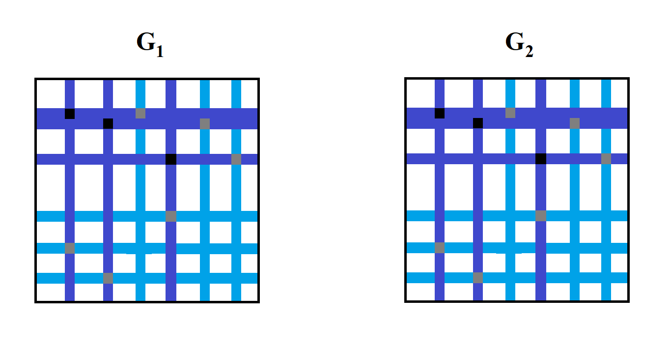
Figure 2. A visualization of a perfect pair of adjacent multigraphs $G_{1}$, $G_{2}$ (for $d=3$). The graphs are represented by their adjacency matrices. The elements colored in black correspond to multiedges. The elements in gray are edges incident to the multiedges. The rows and columns colored in dark blue correspond to left and right vertices incident to multiedges. Those colored in light blue correspond to left and right vertices adjacent to vertices incident to some multiedges. The edges (matrix elements) participating in the simple switching connecting $G_{1}$ and $G_{2}$ must lie outside the colored subset.

As we will see later, $\mathcal{C}_{n,d}(k)$ forms a vast majority in the set of couples of adjacent graphs in ${\rm Cat}_{n,d}(k)\times{\rm Cat}_{n,d}(k)$, and are the main “contributors” to the Dirichlet form. The next proposition establishes a property crucial for us: there is a natural coupling between the $s$–neighborhoods of two adjacent graphs from $\mathcal{C}_{n,d}(k)$.

Proposition 5.2 (Matching of $s$–neighborhoods of perfect pairs).

Let $1\leq k\leq{\mathfrak{m}}$ and $(G_{1},G_{2})\in\mathcal{C}_{n,d}(k)$. Then there is a bijective mapping $\psi_{G_{1},G_{2}}:{\mathcal{S}\mathcal{N}}(G_{1})\to{\mathcal{S}\mathcal{N}}(G_{2})$ such that

$$\mbox{${\rm dist}(G,\psi_{G_{1},G_{2}}(G))=1$ for all $G\in{\mathcal{S}\mathcal{N}}(G_{1})$}.$$

Proof.

Let $1\leq k\leq{\mathfrak{m}}$, $(G_{1},G_{2})\in\mathcal{C}_{n,d}(k)$ and $\Phi=\langle i,i^{\prime},j,j^{\prime}\rangle$ be the switching used to get $G_{2}$ from $G_{1}$. Let $G\in{\mathcal{S}\mathcal{N}}(G_{1})$ and $\Phi_{1},\ldots,\Phi_{k}$ be a sequence of switchings such that $G=\Phi_{k}\circ\ldots\circ\Phi_{1}(G_{1})$. Recall that this collection is uniquely determined, up to the ordering (see Lemma 3.5). Let us note that by the assumptions on the vertices of $\Phi$ and the definition of a simple path, the locations $(i,j^{\prime})$ and $(i^{\prime},j)$ cannot be used by any of the switchings $\Phi_{1},\ldots,\Phi_{k}$ (we recall that, according to our convention, ${\rm Adj}(G_{1})_{ij^{\prime}}={\rm Adj}(G_{1})_{i^{\prime}j}=0$). Indeed, if that was the case, it would necessarily imply that $i$ or $j^{\prime}$ (resp. $i^{\prime}$ or $j$) is incident to a multiedge in $G_{1}$. We will consider several cases:

1. None of the switchings used in $\Phi_{1},\ldots,\Phi_{k}$ involve any of the edges $(i,j)$ or $(i^{\prime},j^{\prime})$. Then we set $\psi_{G_{1},G_{2}}(G)$ to be $\Phi(G)$. Thus, $G^{\prime}=\psi_{G_{1},G_{2}}(G)$ is adjacent to $G$; moreover, since $\Phi$ does not operate on any common elements with $\{\Phi_{1},\ldots,\Phi_{k}\}$, the switchings commute, namely, we have

   $$\Phi_{k}\circ\ldots\circ\Phi_{1}(G_{2})=\Phi_{k}\circ\ldots\circ\Phi_{1}\circ\Phi(G_{1})=\Phi\circ(\Phi_{k}\circ\ldots\circ\Phi_{1}(G_{1}))=G^{\prime},$$

   whence $G^{\prime}$ belongs to ${\mathcal{S}\mathcal{N}}(G_{2})$.

2. Exactly one of the two edges $(i,j)$ or $(i^{\prime},j^{\prime})$ is operated on by one of the switchings $\Phi_{1},\ldots,\Phi_{k}$. Without loss of generality, we suppose that this edge is $(i,j)$. Let $1\leq s\leq k$ be such that the switching $\Phi_{s}=\langle i_{s},i_{s}^{\prime},j_{s},j_{s}^{\prime}\rangle$ operates on the edge $(i,j)$, where $(i_{s},j_{s})$ is a multiedge in $G_{1}$. Then necessarily $i=i_{s}^{\prime}$ and $j=j_{s}^{\prime}$. Note that, by the assumptions on $i,i^{\prime},j,j^{\prime}$, the locations $(i_{s},j^{\prime})$ and $(i^{\prime},j_{s})$ are edges neither in $G_{1}$ nor $G_{2}$, and they cannot be used by any of the switchings $\Phi_{1},\ldots,\Phi_{k}$. Indeed, if $(i_{s},j^{\prime})$ (resp. $(i^{\prime},j_{s})$) was an edge, it would imply that $j^{\prime}$ (resp. $i^{\prime}$) is adjacent to the vertex $i_{s}$ (resp. $j_{s}$) which is incident to a multiedge. Moreover, if the location $(i_{s},j^{\prime})$ (resp. $(i^{\prime},j_{s})$) was used by any of the switchings $\Phi_{1},\ldots,\Phi_{k}$, then it would imply that either $i_{s}$ (resp. $j_{s}$) is incident to more than one multiedge or $j^{\prime}$ (resp. $i^{\prime}$) is incident to a multiedge.

   Define $\psi_{G_{1},G_{2}}(G)$ to be the switching $\langle i_{s},i^{\prime},j,j^{\prime}\rangle$ applied to $G$; set $G^{\prime}=\psi_{G_{1},G_{2}}(G)$. It is not difficult to check that $G^{\prime}=\Phi_{k}^{\prime}\circ\ldots\circ\Phi_{1}^{\prime}(G_{2})$ where $\Phi_{s}^{\prime}=\langle i_{s},i,j_{s},j^{\prime}\rangle$ and $\Phi_{r}^{\prime}=\Phi_{r}$ for every $r\neq s$. Therefore $G^{\prime}=\psi_{G_{1},G_{2}}(G)\in{\mathcal{S}\mathcal{N}}(G_{2})$ and is adjacent to $G$. See Figure 3.

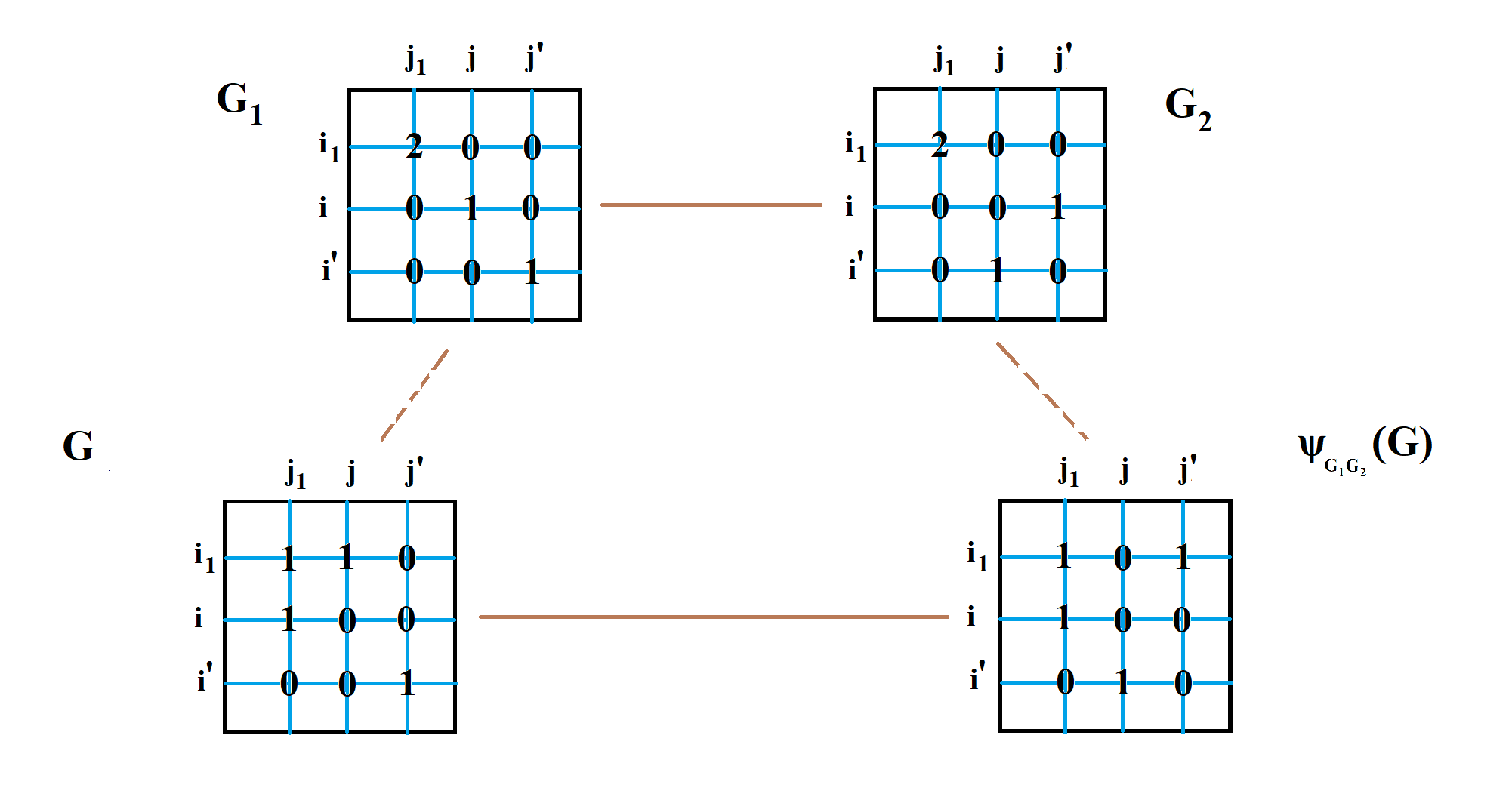
   Figure 3. Construction of a bijective mapping between $s$–neighborhoods of $G_{1}$ and $G_{2}$, case (2). The graphs are represented by their adjacency matrices. In the drawing, the switching $\Phi_{1}=\langle i_{1},i,j_{1},j\rangle$ operates on $(i,j)$. The corresponding switching for $G_{2}$ is $\Phi_{1}^{\prime}=\langle i_{1},i,j_{1},j^{\prime}\rangle$.

   

3. Suppose that both edges $(i,j)$ and $(i^{\prime},j^{\prime})$ are operated on by the switchings $\Phi_{1},\ldots,\Phi_{k}$. This means that there exist two indices $1\leq s_{1},s_{2}\leq k$ such that $\Phi_{s_{1}}=\langle i_{s_{1}},i_{s_{1}}^{\prime},j_{s_{1}},j_{s_{1}}^{\prime}\rangle$ (resp. $\Phi_{s_{2}}=\langle i_{s_{2}},i_{s_{2}}^{\prime},j_{s_{2}},j_{s_{2}}^{\prime}\rangle$) operates on $(i,j)$ (resp. $(i^{\prime},j^{\prime})$), where $(i_{s_{1}},j_{s_{1}})$ and $(i_{s_{2}},j_{s_{2}})$ are multiedges in $G_{1}$. Thus, $i=i_{s_{1}}^{\prime}$, $j=j_{s_{1}}^{\prime}$, $i^{\prime}=i_{s_{2}}^{\prime}$, $j^{\prime}=j_{s_{2}}^{\prime}$.

   Note that the locations $(i_{s_{1}},j^{\prime})$, $(i^{\prime},j_{s_{1}})$, $(i_{s_{2}},j)$, $(i,j_{s_{2}})$ are edges neither in $G_{1}$ nor $G_{2}$ since otherwise, this would imply (in the same order) that $j^{\prime}$, $i^{\prime}$, $j$, $i$ are adjacent to a vertex incident to a multiedge. Moreover, these locations could not have been used in any of the switchings $\Phi_{1},\ldots,\Phi_{k}$ since otherwise, this would imply (in the same order) that either $i_{s_{1}}$, $j_{s_{1}}$, $i_{s_{2}}$, $j_{s_{2}}$ are incident to more than one multiedge or that $j^{\prime}$, $i^{\prime}$, $j$, $i$ are incident to a multiedge.

   Define $\psi_{G_{1},G_{2}}(G)$ to be the switching $\langle i_{s_{1}},i_{s_{2}},j,j^{\prime}\rangle$ applied to $G$; set $G^{\prime}=\psi_{G_{1},G_{2}}(G)$. Note that $G^{\prime}=\Phi_{k}^{\prime}\circ\ldots\circ\Phi_{1}^{\prime}(G_{2})$ where $\Phi_{s_{1}}^{\prime}=\langle i_{s_{1}},i,j_{s_{1}},j^{\prime}\rangle$ and $\Phi_{s_{2}}^{\prime}=\langle i_{s_{2}},i^{\prime},j_{s_{2}},j\rangle$ while $\Phi_{r}^{\prime}=\Phi_{r}$ for any $r\neq s_{1},s_{2}$. Therefore $G^{\prime}=\psi_{G_{1},G_{2}}(G)\in{\mathcal{S}\mathcal{N}}(G_{2})$ and is adjacent to $G$. See Figure 4.

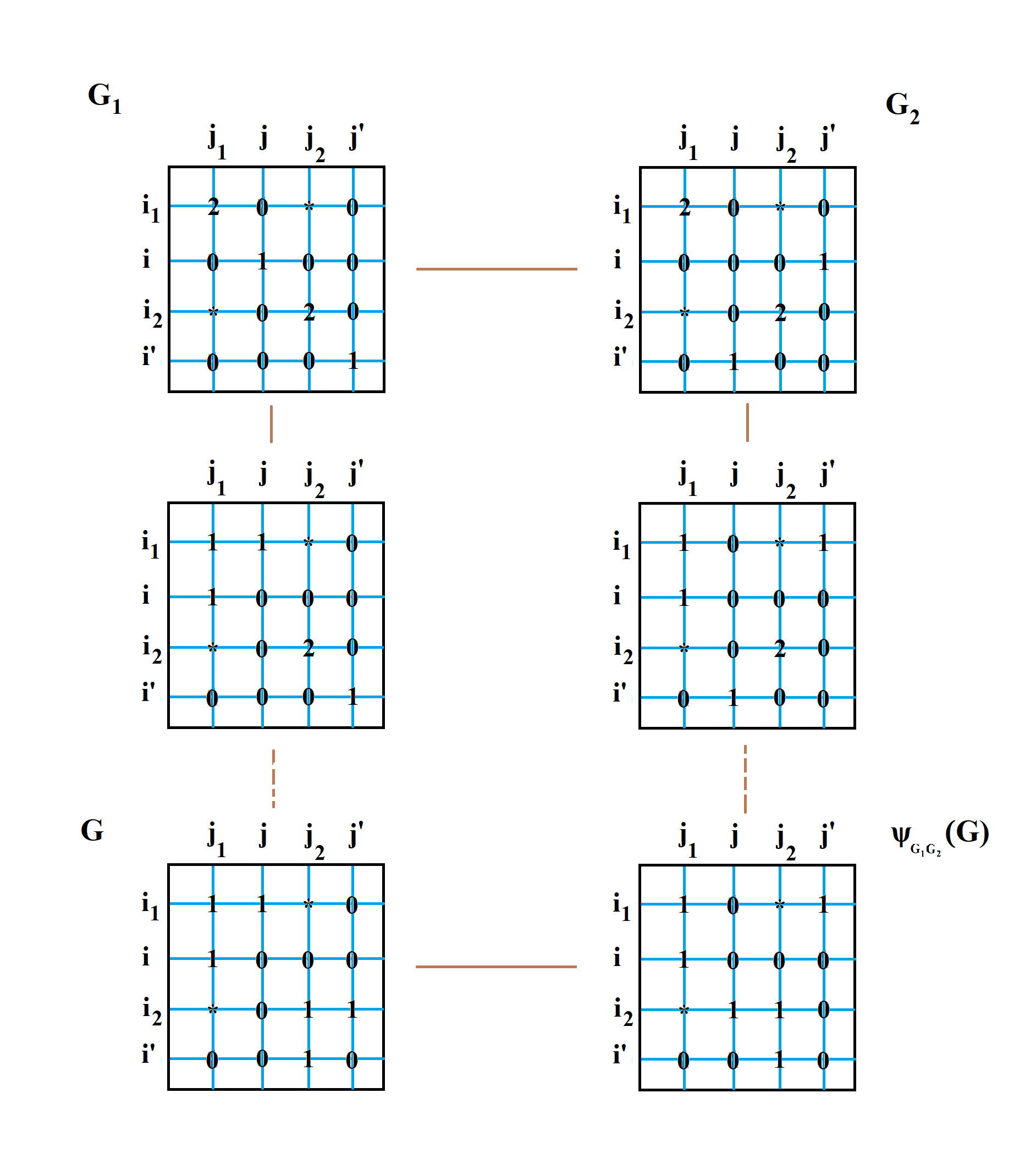
   Figure 4. Construction of a bijective mapping between $s$–neighborhoods of $G_{1}$ and $G_{2}$, case (3). The graphs are represented by their adjacency matrices. In the drawing, the switching $\Phi_{1}=\langle i_{1},i,j_{1},j\rangle$ operates on $(i,j)$, and the switching $\Phi_{2}=\langle i_{2},i^{\prime},j_{2},j^{\prime}\rangle$ operates on $(i^{\prime},j^{\prime})$. The corresponding switchings for the graph $G_{2}$ are $\Phi_{1}^{\prime}=\langle i_{1},i,j_{1},j^{\prime}\rangle$ and $\Phi_{2}^{\prime}=\langle i_{2},i^{\prime},j_{2},j\rangle$.

   

With the above definition, it is not difficult to check that $\psi_{G_{1},G_{2}}\circ\psi_{G_{2},G_{1}}$ (resp. $\psi_{G_{2},G_{1}}\circ\psi_{G_{1},G_{2}}$) is the identity operator on ${\mathcal{S}\mathcal{N}}(G_{2})$ (resp. ${\mathcal{S}\mathcal{N}}(G_{1})$). Moreover, we have ${\rm dist}(G,\psi_{G_{1},G_{2}}(G))=1$ for all $G\in{\mathcal{S}\mathcal{N}}(G_{1})$. This finishes the proof. ∎

Remark 5.3.

In what follows, we always refer to $\psi_{G_{1},G_{2}}$ constructed in the above proposition as the bijective mapping between ${\mathcal{S}\mathcal{N}}(G_{1})$ and ${\mathcal{S}\mathcal{N}}(G_{2})$.

It turns out that the above procedure can be reversed in the following sense.

Proposition 5.4 (Matching of perfect pairs).

Let $1\leq k\leq{\mathfrak{m}}$ and $G_{1}\in{\rm Cat}_{n,d}(k)$. Let $G\in{\mathcal{S}\mathcal{N}}(G_{1})$ and let $G^{\prime}\in\Omega^{B}_{n}(d)$ be adjacent to $G$. Then there exists at most one multigraph $G_{2}\in{\rm Cat}_{n,d}(k)$ such that $(G_{1},G_{2})\in\mathcal{C}_{n,d}(k)$ and $\psi_{G_{1},G_{2}}(G)=G^{\prime}\in{\mathcal{S}\mathcal{N}}(G_{2})$.

Proof.

Let $\Phi_{1}=\langle i_{1},i_{1}^{\prime},j_{1},j_{1}^{\prime}\rangle,\ldots,\Phi_{k}=\langle i_{k},i_{k}^{\prime},j_{k},j_{k}^{\prime}\rangle$ be the unique collection of switchings leading from $G_{1}$ to $G$ (as before, we assume that $(i_{s},j_{s})$ are the multiedges of $G_{1}$) and let $\psi=\langle a,a^{\prime},b,b^{\prime}\rangle$ be the switching used to pass from $G$ to $G^{\prime}$. For any $G_{2}\in{\rm Cat}_{n,d}(k)$ with $(G_{1},G_{2})\in\mathcal{C}_{n,d}(k)$, denote by $\Phi_{G_{1},G_{2}}=\langle i_{G_{1},G_{2}},i_{G_{1},G_{2}}^{\prime},j_{G_{1},G_{2}},j_{G_{1},G_{2}}^{\prime}\rangle$ the simple switching used to pass from $G_{1}$ to $G_{2}$. It follows from the construction of $\psi_{G_{1},G_{2}}$ that the switchings $\psi_{G_{1},G_{2}}$ and $\Phi_{G_{1},G_{2}}$ share the same right vertices. Moreover, the left vertices operated on by $\Phi_{G_{1},G_{2}}$ and $\psi_{G_{1},G_{2}}$, coincide whenever they do not belong to $\{i_{s}\}_{1\leq s\leq k}$.

Suppose there are two graphs $G_{2},G_{2}^{\prime}\in{\rm Cat}_{n,d}(k)$ such that $(G_{1},G_{2}),(G_{1},G_{2}^{\prime})\in\mathcal{C}_{n,d}(k)$ and $G^{\prime}=\psi(G)=\psi_{G_{1},G_{2}}(G)=\psi_{G_{1},G_{2}^{\prime}}(G)$. We will prove that $\Phi_{G_{1},G_{2}}=\Phi_{G_{1},G_{2}^{\prime}}$ which would imply that $G_{2}=G_{2}^{\prime}$. It follows from the above that $\Phi_{G_{1},G_{2}}$ and $\Phi_{G_{1},G_{2}^{\prime}}$ share the same right vertices and these are $b$ and $b^{\prime}$ i.e. $j_{G_{1},G_{2}}=j_{G_{1},G_{2}^{\prime}}=b$ and $j_{G_{1},G_{2}}^{\prime}=j_{G_{1},G_{2}^{\prime}}^{\prime}=b^{\prime}$.

We will consider several cases parallel to the ones in the proof of Proposition 5.2:

1. Neither of the two left vertices $a,a^{\prime}$ belong to $\{i_{s}\}_{1\leq s\leq k}$. This means that $\psi_{G_{1},G_{2}}(G)=\psi_{G_{1},G_{2}^{\prime}}(G)$ is constructed as in the first case of the proof of Proposition 5.2, i.e. $i_{G_{1},G_{2}}=i_{G_{1},G_{2}^{\prime}}=a$, $i_{G_{1},G_{2}}^{\prime}=i_{G_{1},G_{2}^{\prime}}^{\prime}=a^{\prime}$, and $\Phi_{G_{1},G_{2}}=\Phi_{G_{1},G_{2}^{\prime}}=\langle a,a^{\prime},b,b^{\prime}\rangle$.

2. Exactly one of the left vertices $a,a^{\prime}$ belongs to $\{i_{s}\}_{1\leq s\leq k}$. Without loss of generality, we suppose it is $a$. Let $1\leq s\leq k$ be such that $i_{s}=a$. Note that since $a^{\prime}\not\in\{i_{s}\}_{1\leq s\leq k}$, then we have $i_{G_{1},G_{2}}^{\prime}=i_{G_{1},G_{2}^{\prime}}^{\prime}=a^{\prime}$. Necessarily, we are in the second case of Proposition 5.2, i.e. the switching used to pass from $G$ to $G^{\prime}$ is

   $$\psi=\langle i_{s},i_{G_{1},G_{2}}^{\prime},j_{G_{1},G_{2}},j_{G_{1},G_{2}}^{\prime}\rangle=\langle i_{s},i_{G_{1},G_{2}^{\prime}}^{\prime},j_{G_{1},G_{2}^{\prime}},j_{G_{1},G_{2}^{\prime}}^{\prime}\rangle.$$

   Note that the second case of Proposition 5.2 assumes that $\Phi_{s}$ operates on one of the edges $(i_{G_{1},G_{2}},j_{G_{1},G_{2}})$ or $(i_{G_{1},G_{2}}^{\prime},j_{G_{1},G_{2}}^{\prime})=(a^{\prime},b^{\prime})$, i.e. either $(i_{s}^{\prime},j_{s}^{\prime})=(i_{G_{1},G_{2}},b)$ or $(i_{s}^{\prime},j_{s}^{\prime})=(a^{\prime},b^{\prime})$. The latter case is impossible because it would mean that the edge $(a^{\prime},b^{\prime})$ is removed from the graph $G$, so $\psi$ could not be applied to $G$. Thus, $i_{G_{1},G_{2}}=i_{s}^{\prime}$. By the same reasoning we get that $i_{G_{1},G_{2}^{\prime}}=i_{s}^{\prime}$, so $\Phi_{G_{1},G_{2}}=\Phi_{G_{1},G_{2}^{\prime}}=\langle i_{s}^{\prime},a^{\prime},b,b^{\prime}\rangle$.

3. Both left vertices $a,a^{\prime}$ belong to $\{i_{s}\}_{1\leq s\leq k}$. Let $1\leq s_{1},s_{2}\leq k$ be such that $a=i_{s_{1}}$ and $a^{\prime}=i_{s_{2}}$. Note that it is the third case of Proposition 5.2 which could lead to such configuration:

   $$\psi=\langle i_{s_{1}},i_{s_{2}},j_{G_{1},G_{2}},j_{G_{1},G_{2}}^{\prime}\rangle=\langle i_{s_{1}},i_{s_{2}},j_{G_{1},G_{2}^{\prime}},j_{G_{1},G_{2}^{\prime}}^{\prime}\rangle.$$

   Note that the third case assumes that $\Phi_{s_{1}}$ operates on the edge $(i_{G_{1},G_{2}},j_{G_{1},G_{2}})$ and $\Phi_{s_{2}}$ operates on $(i_{G_{1},G_{2}}^{\prime},j_{G_{1},G_{2}}^{\prime})$, i.e. $(i_{s_{1}}^{\prime},j_{s_{1}}^{\prime})=(i_{G_{1},G_{2}},j_{G_{1},G_{2}})$, $(i_{s_{2}}^{\prime},j_{s_{2}}^{\prime})=(i_{G_{1},G_{2}}^{\prime},j_{G_{1},G_{2}}^{\prime})$, so $\Phi_{G_{1},G_{2}}=\langle i_{s_{1}}^{\prime},i_{s_{2}}^{\prime},b,b^{\prime}\rangle$. Similarly, we must have $\Phi_{G_{1},G_{2}^{\prime}}=\langle i_{s_{1}}^{\prime},i_{s_{2}}^{\prime},b,b^{\prime}\rangle$, so $\Phi_{G_{1},G_{2}}=\Phi_{G_{1},G_{2}^{\prime}}$, and the proof is complete.

∎

6. Connections

The goal of this section is to define canonical paths between simple graphs, which will be called connections. As was mentioned in the proof overview, connections will be used when bounding from above the Dirichlet form of the function extension in terms of the Dirichlet form of the original function. Whereas the “main weight” of the Dirichlet form of the extension is comprised by perfect pairs of multigraphs which admit a bijective mapping between their $s$–neighborhoods (see Section 5), the imperfect pairs have to be dealt with differently. We prefer to give a simplistic viewpoint here. Given an imperfect pair of multigraphs $(G_{1}^{\prime},G_{2}^{\prime})$, we will first match all couples $(G_{1},G_{2})$ of simple graphs within the $s$–neighborhoods of $G_{1}^{\prime}$ and $G_{2}^{\prime}$ and then will bound expressions of the form $(f(G_{1})-f(G_{2}))^{2}$, which shall appear in computations, by

$${\rm len}(P)\,\sum_{t=1}^{{\rm len}(P)}(f(P[t])-f(P[t-1]))^{2},$$

where $P$ is a connection between $G_{1}$ and $G_{2}$ — a path starting at $G_{1}$ and ending at $G_{2}$ that is determined not only by $G_{1}$ and $G_{2}$ but also the multigraphs $G_{1}^{\prime},G_{2}^{\prime}$ and thus depends on the entire $4$–tuple ${\mathcal{T}}=(G_{1},G_{1}^{\prime},G_{2},G_{2}^{\prime})$. Connections must be constructed in such a way that in the resulting weighted sum over $4$–tuples

$$\sum\limits_{{\mathcal{T}}}\sum_{t=1}^{{\rm len}(P_{\mathcal{T}})}\mbox{weight}(t,{\mathcal{T}})\;(f(P_{\mathcal{T}}[t])-f(P_{\mathcal{T}}[t-1]))^{2},$$

no pair of adjacent simple graphs receives “too big” total weight, and this is the main difficulty in properly defining them. Connections will also be employed when mapping simple graphs within a common $s$–neighborhood, and in the situation when a multigraph is adjacent to a simple graph which does not belong to its $s$–neighborhood.

Thus, we will deal with three types of connections:

• Type $1$. Paths connecting simple graphs in $s$–neighborhoods of two adjacent multigraphs.

• Type $2$. Paths connecting two simple graphs within the $s$–neighborhood of a given multigraph.

• Type $3$. A path connecting a simple graph within the $s$–neighborhood of a multigraph, and a simple graph adjacent to the multigraph but not contained within its $s$–neighborhood.

Let us introduce a classification on quadruples of graphs. Let ${\mathcal{T}}:=(G_{1},G_{1}^{\prime},G_{2},G_{2}^{\prime})$ be a $4$–tuple of graphs in $\Omega^{B\,C}_{n}(d)$, where $G_{1},G_{2}\in\Omega^{B}_{n}(d)$. We say that ${\mathcal{T}}$ is

• Of type $1$, if $G_{1}\in{\mathcal{S}\mathcal{N}}(G_{1}^{\prime})$, $G_{2}\in{\mathcal{S}\mathcal{N}}(G_{2}^{\prime})$, the two graphs $G_{1}^{\prime}$ and $G_{2}^{\prime}$ are adjacent in $\Omega^{B\,C}_{n}(d)$; $G_{1}^{\prime},G_{2}^{\prime}\in{\rm Cat}_{n,d}([1,{\mathfrak{m}}])$, and the pair $(G_{1}^{\prime},G_{2}^{\prime})$ is not perfect (see Definition 5.1).

• Of type $2$, if $G_{1}\in{\mathcal{S}\mathcal{N}}(G_{1}^{\prime})$, $G_{2}\in{\mathcal{S}\mathcal{N}}(G_{2}^{\prime})$, and $G_{1}^{\prime}=G_{2}^{\prime}\in{\rm Cat}_{n,d}([1,{\mathfrak{m}}])$.

• Of type $3$, if $G_{1}=G_{1}^{\prime}$ is adjacent to $G_{2}^{\prime}\in{\rm Cat}_{n,d}([1,{\mathfrak{m}}])$, and $G_{2}\in{\mathcal{S}\mathcal{N}}(G_{2}^{\prime})$, $G_{1}\notin{\mathcal{S}\mathcal{N}}(G_{2}^{\prime})$.

A $4$–tuple of any of the above three types will be called admissible. We would like to emphasize that the graphs $G_{1}^{\prime}$ and $G_{2}^{\prime}$ for a type $1$ tuple may be of different categories (this may happen if the switching operation between the graphs operates on multiedges). Clearly, in the cases of type $2$ and $3$, $3$–tuples could have been used without any loss of information, but the above convention will allow us to treat all three types in a uniform way whenever possible. The following simple lemma follows directly from the definitions:

Lemma 6.1.

Let ${\mathcal{T}}:=(G_{1},G_{1}^{\prime},G_{2},G_{2}^{\prime})$ be of type $3$. Then necessarily $G_{2}^{\prime}$ has category number $2$, with two multiedges of multiplicity two each, and the simple switching used to produce $G_{1}=G_{1}^{\prime}$ from $G_{2}^{\prime}$, operates on those multiedges.

Proof.

We refer to Figure 5 for illustration. ∎

Figure 5. The structure of a type $3$ tuple ${\mathcal{T}}=(G_{1},G_{1}^{\prime},G_{2},G_{2}^{\prime})$. The graphs are represented by their adjacency matrices.

Let ${\mathcal{T}}:=(G_{1},G_{1}^{\prime},G_{2},G_{2}^{\prime})$ be any admissible $4$–tuple. Denote by $I(G_{2},G_{2}^{\prime})$ the collection of all indices $i\leq n$ such that a simple path leading from $G_{2}^{\prime}$ to $G_{2}$ contains a simple switching involving left vertex $i^{\ell}$. We will partition $I(G_{2},G_{2}^{\prime})$ into two subsets

$$I(G_{2},G_{2}^{\prime})=I_{m}(G_{2},G_{2}^{\prime})\sqcup I_{s}(G_{2},G_{2}^{\prime}),$$

where $I_{m}(G_{2},G_{2}^{\prime})$ is defined as the collection of all left vertices $i^{\ell}$ such that $G_{2}^{\prime}$ has a multiple edge emanating from $i^{\ell}$. Clearly, $I_{s}(G_{2},G_{2}^{\prime})$ then consists of all the left vertices which do not have incident multiple edges and which are employed in the simple switching operations leading from $G_{2}^{\prime}$ to $G_{2}$. We define $I(G_{1},G_{1}^{\prime})=I_{m}(G_{1},G_{1}^{\prime})\sqcup I_{s}(G_{1},G_{1}^{\prime})$ according to the same rules for types $1$ and $2$; let $I_{m}(G_{1},G_{1}^{\prime})=I_{s}(G_{1},G_{1}^{\prime})=\emptyset$ for type $3$ tuples, and let $I({\mathcal{T}}):=I(G_{1},G_{1}^{\prime})\cup I(G_{2},G_{2}^{\prime})$.

Definition 6.2.

We say that an edge $(i,j)$ is $m$–standard with respect to a $4$–tuple ${\mathcal{T}}=(G_{1},G_{1}^{\prime},G_{2},G_{2}^{\prime})$ of type $1$ or $2$ if all of the following conditions are satisfied (see Figure 6):

1. The multiplicity of $(i,j)$ both in $G_{1}^{\prime}$ and $G_{2}^{\prime}$ is $2$;

2. The (unique) left vertex ${\bf i1}\neq i$ with $({\bf i1},j)$ an edge in $G_{1}$ but not an edge in $G_{1}^{\prime}$, is not contained in $I(G_{2},G_{2}^{\prime})$, and

3. The (unique) left vertex ${\bf i2}\neq i$ with $({\bf i2},j)$ an edge in $G_{2}$ but not an edge in $G_{2}^{\prime}$, is not contained in $I(G_{1},G_{1}^{\prime})$;

4. For the unique index ${\bf j2}$ such that $(i,{\bf j2})$ an edge in $G_{2}$ but not an edge in $G_{2}^{\prime}$, the couple $({\bf i1},{\bf j2})$ is not an edge in $G_{1}$ or in $G_{2}$;

5. In case when $G_{1}^{\prime}$ and $G_{2}^{\prime}$ do not coincide, the simple switching operation used to pass from $G_{1}^{\prime}$ to $G_{2}^{\prime}$, does not operate on any of the left vertices $\{i,{\bf i1},{\bf i2}\}$.

For future reference, we provide an illustration in the case when all properties above, except for property 4, are satisfied; see Figure 7.

Denote the set of all $m$–standard edges w.r.t. ${\mathcal{T}}$ by $E_{S}({\mathcal{T}})$ (for type $3$ tuples, we will set $E_{S}({\mathcal{T}}):=\emptyset$). Observe that each $m$–standard edge $(i,j)\in E_{S}({\mathcal{T}})$ naturally defines four numbers (indices), which we will denote by ${\bf i1}(i,{\mathcal{T}})$, ${\bf i2}(i,{\mathcal{T}})$, ${\bf j1}(i,{\mathcal{T}})$, ${\bf j2}(i,{\mathcal{T}})$:

• ${\bf i1}={\bf i1}(i,{\mathcal{T}})$ is the unique left vertex such that the pair of vertices $({\bf i1},i)$ is operated on by a switching in a simple path from $G_{1}^{\prime}$ to $G_{1}$. Note that $({\bf i1},j)$ an edge in $G_{1}$ but not an edge in $G_{1}^{\prime}$;

• ${\bf i2}={\bf i2}(i,{\mathcal{T}})$ is the unique left vertex which, together with $i$, is operated on by a switching in a simple path from $G_{2}^{\prime}$ to $G_{2}$. Again, we note that that $({\bf i2},j)$ an edge in $G_{2}$ but not an edge in $G_{2}^{\prime}$;

• ${\bf j1}={\bf j1}(i,{\mathcal{T}})$ is the unique right vertex such that $(i,{\bf j1})$ an edge in $G_{1}$ but not an edge in $G_{1}^{\prime}$;

• ${\bf j2}={\bf j2}(i,{\mathcal{T}})$ is the unique right vertex such that $(i,{\bf j2})$ an edge in $G_{2}$ but not an edge in $G_{2}^{\prime}$.

Note that the uniqueness of ${\bf i1}(i,{\mathcal{T}})$ and ${\bf i2}(i,{\mathcal{T}})$ follows from the fact that each double edge of $G_{1}^{\prime}$ or $G_{2}^{\prime}$ is uniquely mapped to a generating simple switching for $G_{1}$ and $G_{2}$, i.e. is guaranteed by Lemma 3.5.

Figure 6. A schematic depiction of an $m$–standard edge $(i,j)$ (the multigraphs are represented by their adjacency matrices).

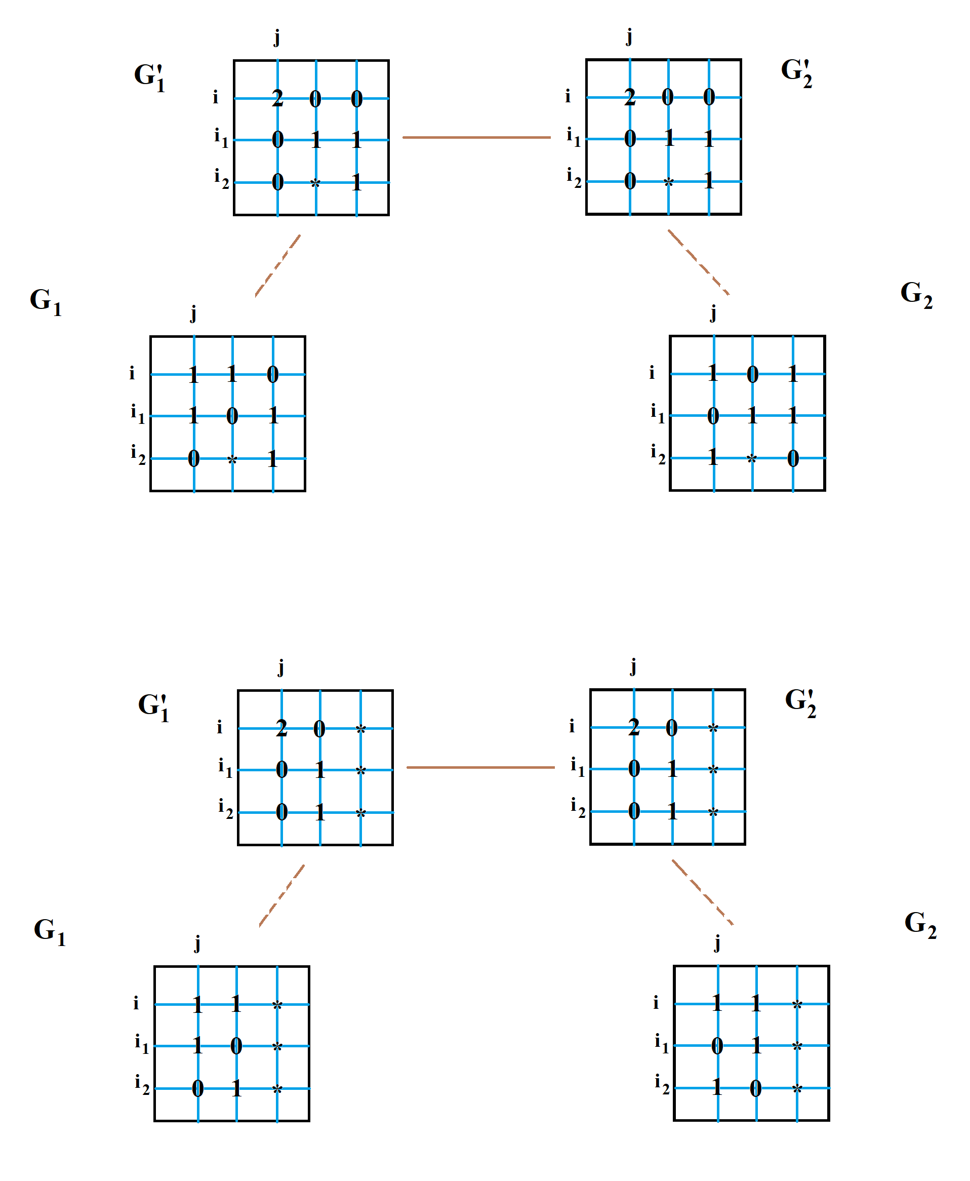
Figure 7. An edge $(i,j)$ satisfying all conditions for an $m$–standard edge, except for property 4 (the multigraphs are represented by their adjacency matrices). More precisely, we illustrate two situations: the first when the edge $({\bf i1},{\bf j2})$ is present in both $G_{1}$ and $G_{2}$, while the second is when the edge is present in $G_{2}$ and absent in $G_{1}$.

For any admissible ${\mathcal{T}}=(G_{1},G_{1}^{\prime},G_{2},G_{2}^{\prime})$, denote

$$I_{ST}({\mathcal{T}}):= \{i\leq n:\;\mbox{$(i,j)\in E_{S}({\mathcal{T}})$ for some $j$}\}\cup\{\tilde{i}\leq n:\;\mbox{there are $i,j\leq n$ such that}$$

$$\hskip 184.9429pt\mbox{$(i,j)\in E_{S}({\mathcal{T}})$ and $\tilde{i}\in\{{\bf i1}(i,{\mathcal{T}}),{\bf i2}(i,{\mathcal{T}})\}$}\}.$$

The set $I_{ST}({\mathcal{T}})$ comprises “standard” left vertices for which a definition of corresponding switching operations leading from $G_{1}$ to $G_{2}$ is relatively straightforward.

Definition 6.3.

Let ${\mathcal{T}}=(G_{1},G_{1}^{\prime},G_{2},G_{2}^{\prime})$ be of type $1$ or $3$.

• We say that the simple switching operation used to transfer between $G_{1}^{\prime}$ and $G_{2}^{\prime}$, is of type A if the left vertices it operates on are not contained in $I({\mathcal{T}})$.

• The switching is of type B if at least one of the left vertices it operates on is in $I({\mathcal{T}})$.

Note that in case of type $3$ tuples, the switching is necessarily of type $B$, whereas in case of type $1$ tuples it can be either type $A$ or type $B$. Moreover, for an admissible tuple ${\mathcal{T}}$ with type A switching, the condition that the pair $(G_{1}^{\prime},G_{2}^{\prime})$ is not perfect, immediately implies that either the vertices the switching operates on are incident to some multiedges of $G_{1}^{\prime},G_{2}^{\prime}$ or those vertices are adjacent to vertices incident to some multiedges (see Definition 5.1).

For any admissible tuple ${\mathcal{T}}=(G_{1},G_{1}^{\prime},G_{2},G_{2}^{\prime})$, denote by $I_{A}({\mathcal{T}})$ the set of left vertices operated on by the simple switching of type $A$ leading from $G_{1}^{\prime}$ to $G_{2}^{\prime}$, whenever such a switching is defined, and set $I_{A}({\mathcal{T}}):=\emptyset$ otherwise.

Let ${\mathcal{T}}=(G_{1},G_{1}^{\prime},G_{2},G_{2}^{\prime})$ be any admissible $4$–tuple. We define the collection of “non-standard” left indices with respect to ${\mathcal{T}}$ as follows. Set $\tilde{I}$ to be empty set if $G_{1}^{\prime}=G_{2}^{\prime}$ (i.e. ${\mathcal{T}}$ is of type $2$) or if the simple switching operating between the two graphs is of type $A$, and let $\tilde{I}$ be the (two) left vertices operated on by the switching from $G_{1}^{\prime}$ to $G_{2}^{\prime}$ if it is of type $B$. Then we set

$$I_{NS}({\mathcal{T}}):=\big{(}I({\mathcal{T}})\setminus I_{ST}({\mathcal{T}})\big{)}\cup\tilde{I}.$$

The set $I_{NS}({\mathcal{T}})$ comprises “non-standard” left indices.

Note that with the above definitions, with each admissible tuple ${\mathcal{T}}=(G_{1},G_{1}^{\prime},G_{2},G_{2}^{\prime})$ we have associated three disjoint sets $I_{ST}({\mathcal{T}})$, $I_{NS}({\mathcal{T}})$ and $I_{A}({\mathcal{T}})$. The canonical path (a connection) between the simple graphs $G_{1}$ and $G_{2}$ will be constructed by combining simple switching operations on $I_{ST}({\mathcal{T}})$, followed by the switching on $I_{A}({\mathcal{T}})$ (if any), and then switchings on the left vertices from $I_{NS}({\mathcal{T}})$. The major issue in constructing the canonical paths is to find a construction procedure which would guarantee that there is no pair of adjacent simple graphs belonging to “too many” connections (in which case we would not be able to efficiently bound the Dirichlet form). The most difficult element of the construction is treatment of the set $I_{NS}({\mathcal{T}})$, because of its relatively complicated structure.

6.1. Structure of the set $I_{NS}({\mathcal{T}})$

The following simple estimates will be important:

Lemma 6.4.

For any admissible tuple ${\mathcal{T}}=(G_{1},G_{1}^{\prime},G_{2},G_{2}^{\prime})$, let $M_{h}$ be the number of multiedges incident to $I_{NS}({\mathcal{T}})$ in $G_{h}^{\prime}$, $h=1,2$. Then necessarily

$$M_{h}\leq|I_{NS}({\mathcal{T}})|,\quad h=1,2.$$

Proof.

The lemma follows from the definition of $I_{NS}({\mathcal{T}})$ and the definition of an $s$–neighborhood. ∎

Lemma 6.5.

For any admissible tuple ${\mathcal{T}}=(G_{1},G_{1}^{\prime},G_{2},G_{2}^{\prime})$, the cardinality of the set of non-standard left indices $I_{NS}({\mathcal{T}})$ satisfies

$$|\{(i,j):\;i\in I_{NS}({\mathcal{T}}),\,(i,j)\mbox{ is an edge in precisely one of the graphs $G_{1},G_{2}$}\}|$$

$$\leq 8\,|I_{NS}({\mathcal{T}})|+4\cdot{\bf 1}_{\{\mbox{$G_{1}^{\prime}$ and $G_{2}^{\prime}$ are adjacent and connected by a type B switching}\}}.$$

Proof.

Denote by $Y$ the set of left vertices operated on by the simple switching connecting $G_{1}^{\prime}$ and $G_{2}^{\prime}$ (we set $Y=\emptyset$ if $G_{1}^{\prime}=G_{2}^{\prime}$). First, take any $i\in I_{NS}({\mathcal{T}})\setminus Y$, and observe that ${\rm row}_{i}({\rm Adj}(G_{1}^{\prime}))={\rm row}_{i}({\rm Adj}(G_{2}^{\prime}))$, and, in particular, the number $M(i)$ of multiedges of $G_{h}^{\prime}$ incident to $i^{\ell}$ is the same for $h=1,2$. Then the number of indices $j$ such that ${\rm mult\,}_{G_{1}}(i,j)\neq{\rm mult\,}_{G_{2}}(i,j)$, can be roughly bounded from above by $4\max(M(i),1)$.

Further, take any $i\in I_{NS}({\mathcal{T}})\cap Y$, and observe that, setting $M_{h}(i)$ to be the number of multiedges of $G_{h}^{\prime}$ incident to $i^{\ell}$ ($h=1,2$), the cardinality of the set

$$\big{\{}j\leq n:\;{\rm mult\,}_{G_{1}}(i,j)\neq{\rm mult\,}_{G_{2}}(i,j)\big{\}}$$

can be roughly estimated from above by $2\max(M_{1}(i),1)+2+2\max(M_{2}(i),1)$.

Summing up over all $i\in I_{NS}({\mathcal{T}})$, we get

$$|\{(i,j):\;i\in I_{NS}({\mathcal{T}}),\,(i,j)\mbox{ is an edge in precisely one of the graphs $G_{1},G_{2}$}\}|$$

$$\leq 4+4|I_{NS}({\mathcal{T}})|+2M_{1}+2M_{2},$$

where $M_{h}$ denotes the number of multiedges incident to $I_{NS}({\mathcal{T}})$ in $G_{h}^{\prime}$, $h=1,2$. It remains to apply Lemma 6.4. ∎

Definition 6.6.

Assume $I_{NS}({\mathcal{T}})\neq\emptyset$. We say that a partition $W_{1}\cup W_{2}\cup\dots\cup W_{h}$ of $I_{NS}({\mathcal{T}})$ is ${\mathcal{T}}$–admissible if all of the following conditions are satisfied:

• for any pair of left vertices $\tilde{i},\hat{i}$ used by a simple switching operation in a simple path leading from $G_{1}^{\prime}$ to $G_{1}$, we have either $\{\tilde{i},\hat{i}\}\subset W_{u}$ for some $u\leq h$ or $\{\tilde{i},\hat{i}\}\cap I_{NS}({\mathcal{T}})=\emptyset$;

• similarly, for any pair of left vertices $\tilde{i},\hat{i}$ used by a simple switching operation in the path from $G_{2}^{\prime}$ to $G_{2}$, either $\{\tilde{i},\hat{i}\}\subset W_{u}$ for some $u\leq h$ or $\{\tilde{i},\hat{i}\}\cap I_{NS}({\mathcal{T}})=\emptyset$;

• additionally, if $G_{1}^{\prime}$ and $G_{2}^{\prime}$ are adjacent and are connected by a type B switching then for the left vertices $\{\tilde{i},\hat{i}\}$ employed by the simple switching operation to transit between $G_{1}^{\prime}$ and $G_{2}^{\prime}$, we have $\{\tilde{i},\hat{i}\}\subset W_{u}$ for some $u\leq h$.

First, the definition of $I_{NS}({\mathcal{T}})$ implies that $\{I_{NS}({\mathcal{T}})\}$ is a ${\mathcal{T}}$–admissible partition. It is not difficult to see that there is a common refinement to all ${\mathcal{T}}$–admissible partitions which is also ${\mathcal{T}}$–admissible, and which we will call the canonical partition of $I_{NS}({\mathcal{T}})$. It will be convenient to fix an order of elements for a canonical partition: we will write $I_{NS}({\mathcal{T}})=W_{1}\sqcup W_{2}\sqcup\dots\sqcup W_{h}$, where $\min W_{q}<\min W_{q+1}$ for all $q<h$. To emphasize dependence on ${\mathcal{T}}$, we will occasionally use notation $W_{1}({\mathcal{T}}),W_{2}({\mathcal{T}}),\dots$. Further, we will adopt a convention that $W_{q}({\mathcal{T}})=\emptyset$ whenever $I_{NS}({\mathcal{T}})$ is empty or the index $q$ is larger than the cardinality of the canonical partition of $I_{NS}({\mathcal{T}})$, so that $I_{NS}({\mathcal{T}})$ can be associated with infinite sequence $(W_{q}({\mathcal{T}}))_{q=1}^{\infty}$.

The canonical partition can be interpreted in the following way. Consider the collection $S$ of all simple switchings operating on left vertices from $I_{NS}({\mathcal{T}})$ and participating in a simple path from $G_{1}^{\prime}$ to $G_{1}$ (if any) or from $G_{2}^{\prime}$ to $G_{2}$, together with the switching between $G_{1}^{\prime}$ and $G_{2}^{\prime}$ if it is of type B. We then connect any two distinct switchings $\phi,\psi\in S$ by an edge whenever they operate on intersecting $2$–subsets of left vertices. Then the canonical partition of $I_{NS}({\mathcal{T}})$ will correspond to partitioning the resulting graph on $S$ into connected components.

It will be crucial for us to have a description of the structure of the canonical partition. Note that a delicate feature of $I_{NS}({\mathcal{T}})$ is that number and location of multiedges of $G_{1}^{\prime}$ and $G_{2}^{\prime}$ incident to $I_{NS}({\mathcal{T}})$ might differ in the case when the simple switching connecting $G_{1}^{\prime}$ and $G_{2}^{\prime}$ operates on some multiedges (in particular, when ${\mathcal{T}}$ is of type $3$).

Lemma 6.7 (Structure of canonical partition for types $1,2$).

Let ${\mathcal{T}}=(G_{1},G_{1}^{\prime},G_{2},G_{2}^{\prime})$ be a tuple of type $1$ or $2$. Assume further that $I_{NS}({\mathcal{T}})$ is non-empty, and let $(W_{q})_{q=1}^{\infty}$ be its canonical partition. Fix any $u$ with $W_{u}\neq\emptyset$, and denote by $M_{u}^{h}$ the number of multiedges of $G_{h}^{\prime}$ incident to $W_{u}$, $h=1,2$. Let $Y$ be the set of left vertices employed in the simple switching operation taking $G_{1}^{\prime}$ to $G_{2}^{\prime}$ (if $G_{1}^{\prime}=G_{2}^{\prime}$ then we set $Y=\emptyset$). Then we have

• If $Y\cap W_{u}=\emptyset$ then necessarily $\max(|W_{u}|-2,1)\leq 2M_{u}^{1}-1=2M_{u}^{2}-1=M_{u}^{1}+M_{u}^{2}-1$;

• If $Y\cap W_{u}\neq\emptyset$ then $Y\subset W_{u}$, and $|W_{u}|\leq 2+M_{u}^{1}+M_{u}^{2}$.

In particular, in either case we have $|W_{u}|\leq 2+M_{u}^{1}+M_{u}^{2}$.

Proof.

First, consider the case $Y\cap W_{u}=\emptyset$. Note that in this case the location of the multiedges incident to left vertices from $W_{u}$, is the same for both graphs $G_{1}^{\prime}$ and $G_{2}^{\prime}$, so necessarily $M_{u}^{1}=M_{u}^{2}$. Further, for each $i\in W_{u}$, denote by $M_{u}(i)$ the number of multiedges of $G_{1}^{\prime}$ (or $G_{2}^{\prime}$) incident to $i$ (observe that $M_{u}(i)$ can only take values $0$ or $1$). Taking into account the definition of a simple path and of $I_{NS}({\mathcal{T}})$, each such left vertex $i$ is associated with a set $S(i,h)$ of left vertices not containing $i$, with $S(i,h)\subset W_{u}$, where $S(i,h)$ are the vertices operated on by simple switchings involving $i^{\ell}$ and participating in generation of the path leading from $G_{h}^{\prime}$ to $G_{h}$, $h=1,2$. Note that, by the conditions on ${\mathcal{T}}$, the set $S(i,h)$ is either empty or has cardinality $1$; $|S(i,h)|=M_{u}(i)$, $h=1,2$. If $\hat{I}$ is the set of all left vertices in $W_{u}$ incident to multiedges then

$$W_{u}=\bigcup_{i\in\hat{I}}\big{(}\{i\}\cup S(i,1)\cup S(i,2)\big{)}.$$

Now, a crucial observation is that we can introduce a total order “$\precsim$” on the vertices in $\hat{I}$ in such a way that

$$\big{(}\{i\}\cup S(i,1)\cup S(i,2)\big{)}\cap\bigcup\limits_{j\in\hat{I},\,j\prec i}\big{(}\{j\}\cup S(j,1)\cup S(j,2)\big{)}\neq\emptyset,\quad i\in\hat{I}\setminus\min\limits_{\precsim}\hat{I}.$$

The last assertion follows from the definition of the canonical partition as a common refinement of all ${\mathcal{T}}$–admissible partitions of $I_{NS}({\mathcal{T}})$: if the condition was not satisfied then it would be possible to split $W_{u}$ into smaller subsets. This property implies that

$$|W_{u}|=\Big{|}\bigcup_{i\in\hat{I}}\big{(}\{i\}\cup S(i,1)\cup S(i,2)\big{)}\Big{|} \leq\sum_{i\in\hat{I}}\big{|}\big{(}\{i\}\cup S(i,1)\cup S(i,2)\big{)}\big{|}-\big{(}|\hat{I}|-1\big{)}$$

$$=\sum_{i\in\hat{I}}\big{|}\big{(}S(i,1)\cup S(i,2)\big{)}\big{|}+1$$

$$\leq 2\sum_{i\in\hat{I}}M_{u}(i)+1=2M^{h}_{u}+1,\quad h=1,2.$$

Thus, $|W_{u}|\leq 2M^{h}_{u}+1$, $h=1,2$. Moreover, since $M_{u}^{h}\geq 1$, $h=1,2$ then necessarily $2M^{h}_{u}-1\geq 1$. Therefore, we get $\max(|W_{u}|-2,1)\leq 2M^{h}_{u}-1$.

Now, consider the case $Y\cap W_{u}\neq\emptyset$, when necessarily $Y\subset W_{u}$. This case is more complicated since the number and location of multiedges incident to $W_{u}$ does not have to be the same for $G_{1}^{\prime}$ and $G_{2}^{\prime}$. Denote by $\hat{I}_{h}$ the set of all left vertices in $W_{u}$ incident to multiedges of $G_{h}^{\prime}$, $h=1,2$, and define $S(i,h)$, $i\in\hat{I}_{h}$, as in the previous case. It will be convenient to set $S(i,h):=\emptyset$ for any $i\in\hat{I}_{3-h}\setminus\hat{I}_{h}$, $h=1,2$, and define $S(i):=\{i\}\cup S(i,1)\cup S(i,2)$, $i\in\hat{I}_{1}\cup\hat{I}_{2}$. We then have

$$W_{u}=Y\cup\bigcup_{i\in\hat{I}_{1}\cup\hat{I}_{2}}\big{(}\{i\}\cup S(i,1)\cup S(i,2)\big{)}=Y\cup\bigcup_{i\in\hat{I}_{1}\cup\hat{I}_{2}}S(i).$$

Let us introduce a “fake” token $\circledast$ and set $S(\circledast):=Y$. Then, again using the definition of the canonical partition, we can claim existence of a total order “$\precsim$” on $\hat{I}:=\hat{I}_{1}\cup\hat{I}_{2}\sqcup\{\circledast\}$, so that

$$S(i)\cap\bigcup\limits_{j\in\hat{I},\,j\prec i}S(j)\neq\emptyset,\quad i\in\hat{I}\setminus\min\limits_{\precsim}\hat{I}.$$

Thus,

$$|W_{u}|\leq\sum\limits_{i\in\hat{I}}|S(i)|-(|\hat{I}|-1)=2+\sum\limits_{i\in\hat{I}_{1}\cup\hat{I}_{2}}|S(i,1)\cup S(i,2)|\leq 2+M_{u}^{1}+M_{u}^{2}.$$

The result follows. ∎

Lemma 6.8 (Structure of canonical partition for type $3$).

Let ${\mathcal{T}}=(G_{1},G_{1}^{\prime},G_{2},G_{2}^{\prime})$ be a tuple of type $3$. Then $I_{NS}({\mathcal{T}})$ is of cardinality $4$, and its canonical partition consists of a single element $W_{1}({\mathcal{T}})$.

Proof.

The structure of $I_{NS}({\mathcal{T}})$ for type $3$ is visualized in Figure 5. ∎

6.2. Definition of a connection

Let us start with statements which provide a path between two bipartite irregular graphs. The first statement will be used for graphs having at least $2$ left vertices; the second one – with at least $4$ left vertices; both satisfying some additional assumptions. The statements will be used to estimate complexity (i.e. number of distinct realizations) of the set of non-standard left vertices $I_{NS}$. A crucial observation is that presence of common neighbors between left vertices reduces the complexity due to the fact that, in our setting, $d$ is less than a small power of $n$ whence most pairs of left vertices are at distance greater than $2$. The statements below will provide certain guarantees regarding existence of common neighbors.

Lemma 6.9.

Let $m\geq 2$, and let $\tilde{G}_{1}\neq\tilde{G}_{2}$ be two simple bipartite graphs on $[m]\sqcup[n]$, such that the degree of every left vertex of each of the graphs is $d\geq 3$, and such that $\deg_{\tilde{G}_{1}}(j^{r})=\deg_{\tilde{G}_{2}}(j^{r})$ for all $j\leq n$. Assume further that the total number of pairs $(i,j)\in[m]\times[n]$ such that $(i,j)$ is an edge in exactly one of the two graphs, is bounded above by $k$. Then there is a path $\tilde{P}$ (formed by simple switchings) on the set of all simple bipartite graphs on $[m]\sqcup[n]$ with left vertex degrees $d$ and right vertex degrees $(\deg_{\tilde{G}_{1}}(j^{r}))_{j=1}^{n}$, satisfying all of the following properties:

1. $\tilde{P}$ starts at $\tilde{G}_{1}$ and ends at $\tilde{G}_{2}$;

2. The length of $\tilde{P}$ is at most $k+2$;

3. Assume additionally that $m\geq 3$. Then for every $t\leq{\rm len}(\tilde{P})$, and the pair $\{i_{1},i_{2}\}$ of left vertices of $\tilde{P}[t-1]$ operated on by the simple switching transforming the graph to $\tilde{P}[t]$, at least one of the following should hold:

   • $i_{1}$ and $i_{2}$ have no common neighbors in $\tilde{P}[t-1]$;

   • there is a left vertex $i\in[m]\setminus\{i_{1},i_{2}\}$ having at least one common neighbor with some vertex in $[m]\setminus\{i\}$ in $\tilde{P}[t-1]$.

Proof.

The case $m=2$, as well as the case when all rows of ${\rm Adj}(\tilde{G}_{1})$ are disjoint, are straightforward and can be checked directly, so we will restrict our attention to the case when $m\geq 3$ and not all rows of ${\rm Adj}(\tilde{G}_{1})$ are disjoint.

We will describe an algorithm which produces a path with the required properties. Denote the set of simple bipartite graphs on $[m]\sqcup[n]$ with left vertex degrees $d$ and right vertex degrees $(\deg_{\tilde{G}_{1}}(j^{r}))_{j=1}^{n}$ by $M$. For any graph $G$ in $M$, let ${\rm disc\,}(G)$ be the total number of pairs $(i,j)\in[m]\times[n]$ such that ${\rm mult\,}_{G}(i,j)\neq{\rm mult\,}_{\tilde{G}_{2}}(i,j)$. The algorithm produces a sequence of graphs $G^{0},G^{1},\dots$ in two stages as follows. We let $G^{0}:=\tilde{G}_{1}$ and set $s:=1$ (the length count).

Stage 1.

Iteration step of Stage $1$. We are given a graph $G^{s-1}$. If

(14) $$\begin{split}&\mbox{there is a triple of distinct left vertices $\{i_{1},i^{(2)},i^{(3)}\}$ such that $i^{(2)}$ and $i^{(3)}$ have}\\ &\mbox{a common neighbor in $G^{s-1}$ and}\;\;{\rm row}_{i_{1}}({\rm Adj}(G^{s-1}))\neq{\rm row}_{i_{1}}({\rm Adj}(\tilde{G}_{2}))\end{split}$$

then we proceed as follows. We choose right vertices $j_{2}\neq j_{1}$ such that ${\rm mult\,}_{G^{s-1}}(i_{1},j_{1})=1$ and ${\rm mult\,}_{G^{s-1}}(i_{1},j_{2})=0$ whereas ${\rm mult\,}_{\tilde{G}_{2}}(i_{1},j_{1})=0$ and ${\rm mult\,}_{\tilde{G}_{2}}(i_{1},j_{2})=1$ (existence of such $j_{1},j_{2}$ follows from the fact that $G^{s-1}$ and $\tilde{G}_{2}$ have the same left degree $d$). Next, since $G^{s-1}$ and $\tilde{G}_{2}$ have the same right degrees sequence, there is necessarily an index $i_{2}\neq i_{1}$ such that ${\rm mult\,}_{G^{s-1}}(i_{2},j_{2})=1$ but ${\rm mult\,}_{\tilde{G}_{2}}(i_{2},j_{2})=0$. At this point we consider two subcases:

• Subcase (a): ${\rm mult\,}_{G^{s-1}}(i_{2},j_{1})=0$. Then we produce $G^{s}$ from $G^{s-1}$ by applying the simple switching on $(i_{1},i_{2},j_{1},j_{2})$. We then set $s:=s+1$ and go to the next iteration.

• Subcase (b): ${\rm mult\,}_{G^{s-1}}(i_{2},j_{1})=1$. In this subcase the switching operation on $(i_{1},i_{2},j_{1},j_{2})$ for the graph $G^{s-1}$ is impossible, and we have to invoke an additional argument. Observe that in this situation there is necessarily an index $i_{3}\notin\{i_{1},i_{2}\}$ such that ${\rm mult\,}_{\tilde{G}_{2}}(i_{3},j_{1})=1$ but ${\rm mult\,}_{G^{s-1}}(i_{3},j_{1})=0$. Further, since both left vertices $i_{3}$ and $i_{2}$ have $d$ neighbors in $G^{s-1}$, there must exist an index $j_{3}\in[n]$ such that ${\rm mult\,}_{G^{s-1}}(i_{3},j_{3})=1$ and ${\rm mult\,}_{G^{s-1}}(i_{2},j_{3})=0$. Then we generate $G^{s}$ from $G^{s-1}$ by applying the simple switching on $(i_{2},i_{3},j_{1},j_{3})$, and produce $G^{s+1}$ from $G^{s}$ via the simple switching on $(i_{1},i_{2},j_{1},j_{2})$ (see Figure 8). We then set $s:=s+2$ and go to the next iteration.

If condition (14) is not satisfied then we complete Stage $1$.

As the output of Stage $1$, we obtain a graph $G^{s-1}$ which does not satisfy condition (14). Termination of Stage $1$ is guaranteed by the following simple observation: whenever $G^{\tilde{s}}$ is produced from $G^{\tilde{s}-1}$ via subcase (a) then we have ${\rm disc\,}(G^{\tilde{s}})\leq{\rm disc\,}(G^{\tilde{s}-1})-2$, while in subcase (b), we get ${\rm disc\,}(G^{\tilde{s}+1})\leq{\rm disc\,}(G^{\tilde{s}-1})-2$. Observe also that at every transition step $G^{\tilde{s}-1}\to G^{\tilde{s}}$ of Stage $1$, there is a left vertex $i$ not operated on by the simple switching leading from $G^{\tilde{s}-1}$ to $G^{\tilde{s}}$, which has a common neighbor with $[m]\setminus\{i\}$ in $G^{\tilde{s}-1}$. If $G^{s-1}=\tilde{G}_{2}$ then the path construction is complete. Otherwise, we go to Stage $2$ of the algorithm.

Stage 2. We are given a graph $G^{s-1}$ which does not satisfy (14). In view of our initial assumption (not all rows of ${\rm Adj}(\tilde{G}_{1})$ are disjoint, hence not all rows of ${\rm Adj}(G^{s-1})$ are disjoint), there is a pair of left vertices $i^{\prime}\neq i^{\prime\prime}$ having a common neighbor in $G^{s-1}$ such that

$${\rm row}_{i}({\rm Adj}(G^{s-1}))={\rm row}_{i}({\rm Adj}(\tilde{G}_{2}))\quad\mbox{for all $i\notin\{i^{\prime},i^{\prime\prime}\}$}.$$

Note that ${\rm row}_{i^{\prime}}({\rm Adj}(G^{s-1}))\neq{\rm row}_{i^{\prime}}({\rm Adj}(\tilde{G}_{2}))$ and ${\rm row}_{i^{\prime\prime}}({\rm Adj}(G^{s-1}))\neq{\rm row}_{i^{\prime\prime}}({\rm Adj}(\tilde{G}_{2}))$. Assume for a moment that there is a right vertex $j$ adjacent to some left vertex $i\notin\{i^{\prime},i^{\prime\prime}\}$ in $G^{s-1}$, together with some vertex in $\{i^{\prime},i^{\prime\prime}\}$. For concreteness, we can suppose that $j$ is adjacent to $i$ and $i^{\prime}$. But since ${\rm row}_{i^{\prime\prime}}({\rm Adj}(G^{s-1}))\neq{\rm row}_{i^{\prime\prime}}({\rm Adj}(\tilde{G}_{2}))$, this would imply that (14) is satisfied. Thus, there is no such right vertex $j$.

Then necessarily for each $i\notin\{i^{\prime},i^{\prime\prime}\}$,

$${\rm supp\,}{\rm row}_{i}({\rm Adj}(G^{s-1}))\cap\big{(}{\rm supp\,}{\rm row}_{i^{\prime}}({\rm Adj}(G^{s-1}))\cup{\rm supp\,}{\rm row}_{i^{\prime\prime}}({\rm Adj}(G^{s-1}))\big{)}=\emptyset,$$

and there is a right vertex $\tilde{j}$ adjacent to $i^{\prime},i^{\prime\prime}$ (and only $i^{\prime},i^{\prime\prime}$) in $G^{s-1}$. Pick arbitrary left vertex $i\notin\{i^{\prime},i^{\prime\prime}\}$ and arbitrary $\hat{j}$ with ${\rm mult\,}_{G^{s-1}}(i,\hat{j})=1$. Then ${\rm mult\,}_{G^{s-1}}(i^{\prime},\hat{j})=0$, ${\rm mult\,}_{G^{s-1}}(i,\tilde{j})=0$, and so the simple switching on $(i,i^{\prime},\hat{j},\tilde{j})$ is admissible. Let $G^{s}$ be the graph obtained from $G^{s-1}$ via this switching. Now, consider a restriction of $G^{s}$ to the vertex set $\{i^{\prime},i^{\prime\prime}\}\sqcup([n]\setminus\{\tilde{j},\hat{j}\})$, and observe that both left and right degrees of $G^{s}[\{i^{\prime},i^{\prime\prime}\}\sqcup([n]\setminus\{\tilde{j},\hat{j}\})]$ and $\tilde{G}_{2}[\{i^{\prime},i^{\prime\prime}\}\sqcup([n]\setminus\{\tilde{j},\hat{j}\})]$ are the same. We shall apply iteratively simple switching operations restricted to $\{i^{\prime},i^{\prime\prime}\}\sqcup([n]\setminus\{\tilde{j},\hat{j}\})$ to obtain a graph $G^{\tilde{s}}$ from $G^{s}$ such that

$$G^{\tilde{s}}[\{i^{\prime},i^{\prime\prime}\}\sqcup([n]\setminus\{\tilde{j},\hat{j}\})]=\tilde{G}_{2}[\{i^{\prime},i^{\prime\prime}\}\sqcup([n]\setminus\{\tilde{j},\hat{j}\})],$$

whereas

$${\rm Adj}(G^{\tilde{s}})_{uv}={\rm Adj}(G^{s})_{uv},\quad(u,v)\notin\{i^{\prime},i^{\prime\prime}\}\times([n]\setminus\{\tilde{j},\hat{j}\}).$$

Since the transformed graphs have two left vertices, both of degrees $d-1$, the switching operations are straightforward; moreover, in view of the above remarks for Stage $1$, we can guarantee that $\tilde{s}-1\leq k$. Further, it is not difficult to see that the only four locations where the entries of ${\rm Adj}(G^{\tilde{s}})$ and ${\rm Adj}(\tilde{G}_{2})$ do not agree are $(i,\hat{j})$, $(i,\tilde{j})$, $(i^{\prime},\hat{j})$, $(i^{\prime},\tilde{j})$. Applying the simple switching operation on these entries, we obtain the graph $G^{\tilde{s}+1}=\tilde{G}_{2}$ (see Figure 9). Thus, the total length of the path does not exceed $k+2$. Note also that in view of our construction procedure, at every step there existed a left vertex not participating in the simple switching which has a common neighbor with its complement in $[m]$. ∎

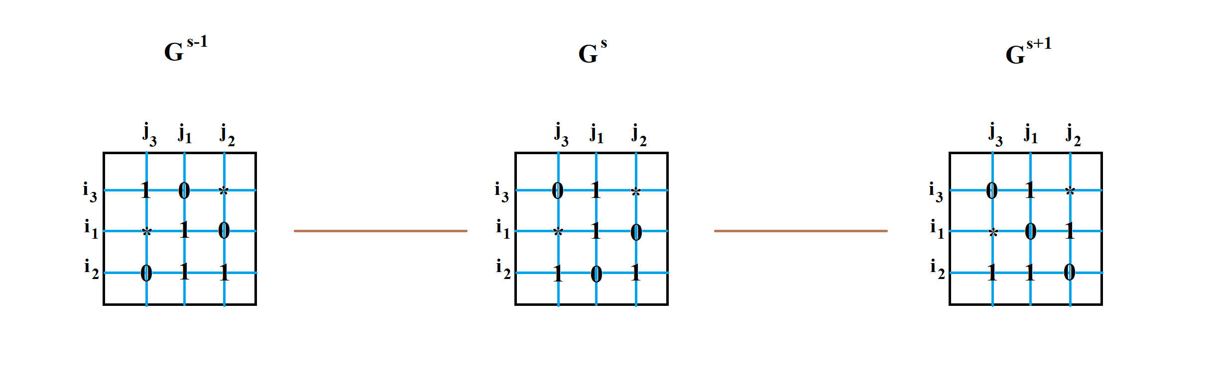
Figure 8. Proof of Lemma 6.9, Stage $1$, Subcase (b).

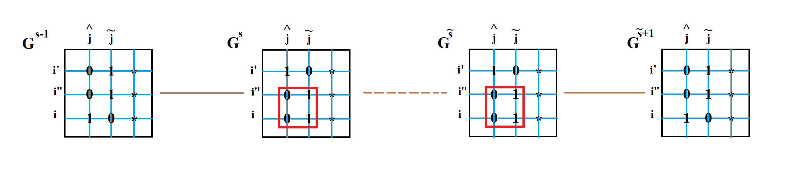
Figure 9. Proof of Lemma 6.9, Stage $2$. The graph $G^{s}$ is obtained from $G^{s-1}$ by “relocating” $1$ within the graphs’ adjacency matrix from position $(i^{\prime},\tilde{j})$ to $(i,\tilde{j})$. Then, necessary switchings are performed on rows $i^{\prime}$ and $i^{\prime\prime}$, leaving the quadruple of elements at the intersection of rows $i^{\prime},i^{\prime\prime}$ and columns $\tilde{j},\hat{j}$ intact. As the last step, the correct positions of elements in the square are “restored”.

Lemma 6.10.

Let $m\geq 4$, and let $\tilde{G}_{1}\neq\tilde{G}_{2}$ be two simple bipartite graphs on $[m]\sqcup[n]$, such that the degree of every left vertex of each of the graphs is $d\geq 3$, and such that $\deg_{\tilde{G}_{1}}(j^{r})=\deg_{\tilde{G}_{2}}(j^{r})$ for all $j\leq n$. Assume that the total number of pairs $(i,j)\in[m]\times[n]$ such that $(i,j)$ is an edge in exactly one of the two graphs, is bounded above by $k$. Assume additionally that for each $h=1,2$, there is a couple of distinct left vertices $i^{(1)}_{h},i^{(2)}_{h}$ such that $i^{(1)}_{h}$ has a common neighbor with $[m]\setminus\{i^{(1)}_{h},i^{(2)}_{h}\}$ in $\tilde{G}_{h}$, and $i^{(2)}_{h}$ has a common neighbor with $[m]\setminus\{i^{(2)}_{h}\}$ in $\tilde{G}_{h}$. Then there is a path $\tilde{P}$ (formed by simple switchings) on the set of all simple bipartite graphs on $[m]\sqcup[n]$ with left vertex degrees $d$ and right vertex degrees $(\deg_{\tilde{G}_{1}}(j^{r}))_{j=1}^{n}$, satisfying all of the following properties:

1. $\tilde{P}$ starts at $\tilde{G}_{1}$ and ends at $\tilde{G}_{2}$;

2. The length of $\tilde{P}$ is at most $C_{\text{\tiny\ref{l: 2095203598305298 bis}}}k$;

3. For every $t\leq{\rm len}(\tilde{P})$, and the pair $\{i_{1},i_{2}\}$ of left vertices of $\tilde{P}[t-1]$ operated on by the simple switching transforming the graph to $\tilde{P}[t]$, there exists a pair of distinct left vertices $\{i_{t}^{\prime},i_{t}^{\prime\prime}\}$ disjoint from $\{i_{1},i_{2}\}$ such that $i_{t}^{\prime}$ has a common neighbor with $[m]\setminus\{i_{t}^{\prime}\}$ and $i_{t}^{\prime\prime}$ has a common neighbor with $[m]\setminus\{i_{t}^{\prime},i_{t}^{\prime\prime}\}$ in the graph $\tilde{P}[t-1]$.

Here, $C_{\text{\tiny\ref{l: 2095203598305298 bis}}}=3/2$.

Proof.

The proof strategy is similar to that of Lemma 6.9 but involves more cases. As in the previous proof, we denote the set of simple bipartite graphs on $[m]\sqcup[n]$ with left vertex degrees $d$ and right vertex degrees $(\deg_{\tilde{G}_{1}}(j^{r}))_{j=1}^{n}$ by $M$, and for any graph $G$ in $M$, let ${\rm disc\,}(G)$ be the total number of pairs $(i,j)\in[m]\times[n]$ such that ${\rm mult\,}_{G}(i,j)\neq{\rm mult\,}_{\tilde{G}_{2}}(i,j)$.

We let $G^{0}:=\tilde{G}_{1}$ and $s:=1$.

Iteration step. We are given a graph $G^{s-1}$ having the following property:

(15) $$\begin{split}&\mbox{there is a couple of distinct left vertices $i^{(1)}_{s},i^{(2)}_{s}$ such that}\\ &\mbox{$i^{(1)}_{s}$ has a common neighbor with $[m]\setminus\{i^{(1)}_{s},i^{(2)}_{s}\}$, and}\\ &\mbox{$i^{(2)}_{s}$ has a common neighbor with $[m]\setminus\{i^{(2)}_{s}\}$ in $G^{s-1}$.}\end{split}$$

If $G^{s-1}=\tilde{G}_{2}$ then we are done. Thus, assume that $G^{s-1}\neq\tilde{G}_{2}$. Then there is a left vertex $i_{1}$ and two right vertices $j_{2}\neq j_{1}$ such that ${\rm mult\,}_{G^{s-1}}(i_{1},j_{1})=1$ and ${\rm mult\,}_{G^{s-1}}(i_{1},j_{2})=0$ while ${\rm mult\,}_{\tilde{G}_{2}}(i_{1},j_{1})=0$ and ${\rm mult\,}_{\tilde{G}_{2}}(i_{1},j_{2})=1$. Since $G^{s-1}$ and $\tilde{G}_{2}$ have the same right degrees sequence, there is necessarily a left index $i_{2}\neq i_{1}$ such that ${\rm mult\,}_{G^{s-1}}(i_{2},j_{2})=1$ but ${\rm mult\,}_{\tilde{G}_{2}}(i_{2},j_{2})=0$. We shall consider several subcases.

1. Assume that ${\rm mult\,}_{G^{s-1}}(i_{2},j_{1})=0$.

   1. Assume there are two distinct left vertices $i^{\prime}_{s},i^{\prime\prime}_{s}\in[m]\setminus\{i_{1},i_{2}\}$ such that $i_{s}^{\prime\prime}$ has a common neighbor with $[m]\setminus\{i_{s}^{\prime},i_{s}^{\prime\prime}\}$ and $i_{s}^{\prime}$ has a common neighbor with $[m]\setminus\{i_{s}^{\prime}\}$ in $G^{s-1}$. In this case, we perform the simple switching on $(i_{1},i_{2},j_{1},j_{2})$ to produce the graph $G^{s}$. Observe that the switching preserves the property of vertices $i_{s}^{\prime},i_{s}^{\prime\prime}$ in the graph $G^{s}$ (i.e. $i_{s}^{\prime\prime}$ has a common neighbor with $[m]\setminus\{i_{s}^{\prime},i_{s}^{\prime\prime}\}$ and $i_{s}^{\prime}$ has a common neighbor with $[m]\setminus\{i_{s}^{\prime}\}$ in $G^{s}$), and that ${\rm disc\,}(G^{s})\leq{\rm disc\,}(G^{s-1})-2$. Set $s:=s+1$ and go to the next iteration.

      
      

      We observe that in all subcases below which assume that the assertion in 1a is not true, there must exist a left vertex $i_{3}\notin\{i_{1},i_{2}\}$ which has a common neighbor with $[m]\setminus\{i_{3}\}$, such that no vertex $v$ in $[m]\setminus\{i_{1},i_{2},i_{3}\}$ has a common neighbor with $\{i_{1},i_{2}\}$.

      
      

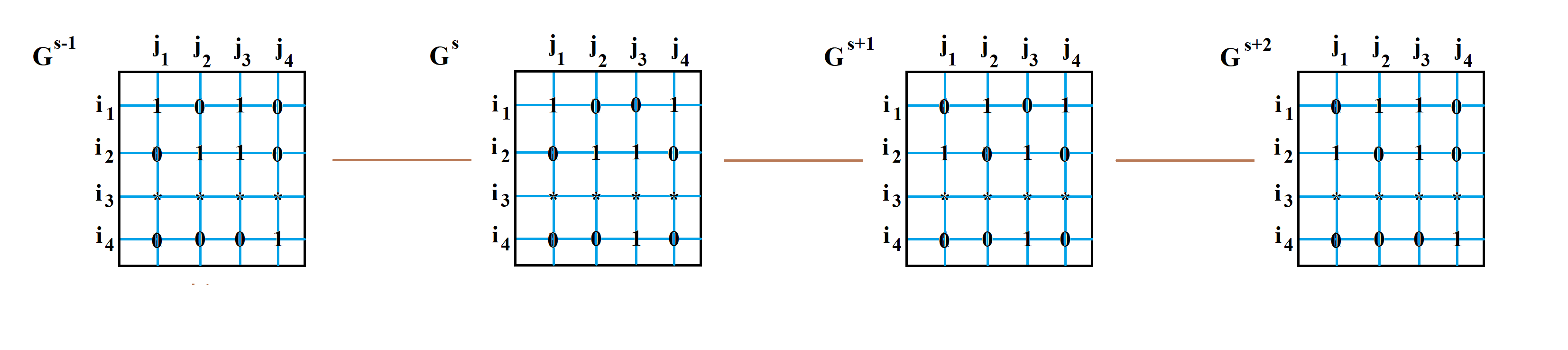
Figure 10. Proof of Lemma 6.10, Subcase 1b.

   2. Assume the assertion in 1a is not true, and the vertices $i_{1}$ and $i_{2}$ have a common neighbor $j_{3}$ in $G^{s-1}$. Pick any left vertex $i_{4}\in[m]\setminus\{i_{1},i_{2},i_{3}\}$. Then necessarily $i_{4}$ and $\{i_{1},i_{2}\}$ do not have common neighbors (because otherwise we fall into case 1a). Let $j_{4}$ be any right vertex such that ${\rm mult\,}_{G^{s-1}}(i_{4},j_{4})=1$. Then necessarily ${\rm mult\,}_{G^{s-1}}(i_{1},j_{4})=0$. Now, we produce the graph $G^{s}$ from $G^{s-1}$ with a switching on $(i_{1},i_{4},j_{3},j_{4})$, then obtain $G^{s+1}$ from $G^{s}$ by a switching on $(i_{1},i_{2},j_{1},j_{2})$, and finally “return” the configuration of $i_{4}$–th neighborhood by switching on $(i_{1},i_{4},j_{4},j_{3})$ to obtain $G^{s+2}$ from $G^{s+1}$. It can be easily checked that ${\rm disc\,}(G^{s+2})\leq{\rm disc\,}(G^{s-1})-2$, and that the graph $G^{s+2}$ satisfies condition (15). Moreover, for each transition $G^{s-1}\to G^{s}$, $G^{s}\to G^{s+1}$, $G^{s+1}\to G^{s+2}$, the property 3 is satisfied (see Figure 10). Set $s:=s+3$ and go to the next step.

      
      

      For future notice, let us explore what the negation of 1a and 1b implies. Let $i^{(1)}_{s},i^{(2)}_{s}$ be the couple of vertices from (15). Note that since we are not in subcase 1a, at least one of $i^{(1)}_{s},i^{(2)}_{s}$ must belong to $\{i_{1},i_{2}\}$, that is, either $i_{1}$ or $i_{2}$ has a common neighbor with some vertex in $[m]\setminus\{i_{1},i_{2}\}$ (at this moment, we applied a negation of 1b). This vertex in $[m]\setminus\{i_{1},i_{2}\}$ having a common neighbor with $\{i_{1},i_{2}\}$, must be unique, and it must be $i_{3}$, because, again, otherwise we would be in Subcase 1a. No vertex in $[m]\setminus\{i_{1},i_{2},i_{3}\}$ has any common neighbors with its complement in $[m]$, but, as (15) must still hold and $i_{1}$ and $i_{2}$ do not have common neighbors, we discover the following necessary conditions on $G^{s-1}$: $i_{3}$ has common neighbors with both $i_{1}$ and $i_{2}$; $i_{1}$ and $i_{2}$ do not have any common neighbors; each vertex $v$ in $[m]\setminus\{i_{1},i_{2},i_{3}\}$ does not have any common neighbors with $[m]\setminus\{v\}$ in $G^{s-1}$.

      
      

   3. Assume the assertions in 1a and 1b are not true, and there is a vertex $u\in[m]\setminus\{i_{1},i_{2},i_{3}\}$ such that ${\rm row}_{u}({\rm Adj}(G^{s-1}))\neq{\rm row}_{u}({\rm Adj}(\tilde{G}_{2}))$. Let $j^{\prime}$ and $j^{\prime\prime}$ be two right vertices so that ${\rm mult\,}_{G^{s-1}}(u,j^{\prime})=1$ and ${\rm mult\,}_{G^{s-1}}(u,j^{\prime\prime})=0$ while ${\rm mult\,}_{\tilde{G}_{2}}(u,j^{\prime})=0$ and ${\rm mult\,}_{\tilde{G}_{2}}(u,j^{\prime\prime})=1$. Since $G^{s-1}$ and $\tilde{G}_{2}$ have the same right degrees sequence, there is necessarily a left index $q\neq u$ such that ${\rm mult\,}_{G^{s-1}}(q,j^{\prime\prime})=1$ but ${\rm mult\,}_{\tilde{G}_{2}}(q,j^{\prime\prime})=0$. Note also that in view of our assumption on $u$ we necessarily have ${\rm mult\,}_{G^{s-1}}(q,j^{\prime})=0$. Then we simply apply Subcase 1a up to vertex relabelling, namely we perform the simple switching on $(u,q,j^{\prime},j^{\prime\prime})$ to produce graph $G^{s}$ from $G^{s-1}$. It is easy to see, using the above assumptions on $\{i_{1},i_{2},i_{3}\}$ that the required conditions on the switching and the graph $G^{s}$ are fulfilled. Set $s:=s+1$ and go to the next iteration.

      
      

      Let us note that negation of 1a, 1b and 1c implies that the rows ${\rm row}_{u}({\rm Adj}(G^{s-1}))$, $u\in[m]\setminus\{i_{1},i_{2},i_{3}\}$, coincide with respective rows of ${\rm Adj}(\tilde{G}_{2})$, and that each $u$ in that set does not have any common neighbors in graph $\tilde{G}_{2}$. At this stage, we apply the crucial property specified in the lemma: “there are $i^{(1)}_{2},i^{(2)}_{2}$ such that $i^{(1)}_{2}$ has a common neighbor with $[m]\setminus\{i^{(1)}_{2},i^{(2)}_{2}\}$, and $i^{(2)}_{2}$ has a common neighbor with $[m]\setminus\{i^{(2)}_{2}\}$ in $\tilde{G}_{2}$”. It, together with the above, implies that each of the vertices $i_{h}$, $h=1,2,3$, must have a common neighbor with $\{i_{1},i_{2},i_{3}\}\setminus\{i_{h}\}$ in the graph $\tilde{G}_{2}$ (and the degree of every right vertex adjacent to $\{i_{1},i_{2},i_{3}\}$ in $\tilde{G}_{2}$ is at most $2$). We shall use this observation in the Subcases 1f and 1g below.

      
      

   4. Assume the assertions in 1a, 1b and 1c are not true, and both right vertices $j_{1}$ and $j_{2}$ have degree one (i.e. adjacent to only one left vertex, $i_{1}$ and $i_{2}$, respectively, in $G^{s-1}$). In this subcase, there exist two right vertices $j_{4}$ and $j_{5}$ not in $\{j_{1},j_{2}\}$ such that $j_{4}$ is adjacent to $i_{1}$ and $i_{3}$, and $j_{5}$ is adjacent to $i_{2}$ and $i_{3}$. We pick any left vertex $i_{4}$ and a right vertex $j_{6}$ such that ${\rm mult\,}_{G^{s-1}}(i_{4},j_{6})=1$ (note that necessarily $i_{4}$ does not have any common neighbors with $i_{1}$, $i_{2}$ or $i_{3}$). The strategy here is very similar to Subcase 1b and consists in applying three switching operations in such a way that the required conditions are not violated by switchings and the graphs $G^{s},G^{s+1},G^{s+2}$. The three consecutive switchings are $(i_{3},i_{4},j_{5},j_{6})$, $(i_{1},i_{2},j_{1},j_{2})$, $(i_{3},i_{4},j_{6},j_{5})$ and the process is reflected in Figure 11. We set $s:=s+3$ and go to the next step.

   5. Assume the assertions in 1a, 1b and 1c are not true, and both $j_{1}$ and $j_{2}$ have degree $2$ in $G^{s-1}$. Pick a pair $(i_{4},j_{4})$ such that $i_{4}\in[m]\setminus\{i_{1},i_{2},i_{3}\}$, and ${\rm mult\,}_{G^{s-1}}(i_{4},j_{4})=1$. The three consecutive switchings are $(i_{3},i_{4},j_{2},j_{4})$, $(i_{1},i_{2},j_{1},j_{2})$, $(i_{3},i_{4},j_{4},j_{2})$ and the switching process is reflected in Figure 12. We set $s:=s+3$ and go to the next step.

   6. Assume the assertions in 1a, 1b and 1c are not true, $j_{1}$ has degree $1$ and $j_{2}$ has degree $2$ in $G^{s-1}$. According to the above remark, $i_{2}$ must have a common neighbor with $\{i_{1},i_{3}\}$ in $\tilde{G}_{2}$, and this common neighbor cannot be $j_{2}$ since ${\rm mult\,}_{\tilde{G}_{2}}(i_{2},j_{2})=0$. Thus, there must exist a right vertex $j_{4}$ of degree two which is adjacent to $i_{2}$ in $\tilde{G}_{2}$. In the graph $G^{s-1}$, $j_{4}$ can be either adjacent to both $i_{2},i_{3}$ or be adjacent to both $i_{1},i_{3}$. In the former sub-subcase, we perform the three-step switching as illustrated in Figure 13 (there, we use an additional edge $(i_{4},j_{5})$ for the switching process to complete). In the latter sub-subcase, our goal shifts from switching $\langle i_{1},i_{2},j_{1},j_{2}\rangle$ to switching $\langle i_{2},i_{1},j_{2},j_{4}\rangle$, again using the three-step process, which is identical, up to the vertex relabelling, to the one described in 1e. Observe that as a result of this procedure we will decrease ${\rm disc\,}(\cdot)$ by at least two since under the assumption that $j_{4}$ is adjacent to both $i_{1},i_{3}$, we have ${\rm mult\,}_{G^{s-1}}(i_{2},j_{4})=0$ while ${\rm mult\,}_{\tilde{G}_{2}}(i_{2},j_{4})=1$. We set $s:=s+3$ and go to the next step.

   7. Assume the assertions in 1a, 1b and 1c are not true, $j_{1}$ has degree $2$ and $j_{2}$ has degree $1$ in $G^{s-1}$. This subcase is identical to the previous one, up to vertex relabelling.

2. Assume that ${\rm mult\,}_{G^{s-1}}(i_{2},j_{1})=1$. In this case there is necessarily an index $i_{3}\notin\{i_{1},i_{2}\}$ such that ${\rm mult\,}_{\tilde{G}_{2}}(i_{3},j_{1})=1$ but ${\rm mult\,}_{G^{s-1}}(i_{3},j_{1})=0$. Further, since both left vertices $i_{3}$ and $i_{2}$ have $d$ neighbors in $G^{s-1}$, there must exist an index $j_{3}\in[n]$ such that ${\rm mult\,}_{G^{s-1}}(i_{3},j_{3})=1$ and ${\rm mult\,}_{G^{s-1}}(i_{2},j_{3})=0$. Again, we consider two subcases.

   1. Assume that there is a vertex $i_{4}\in[m]\setminus\{i_{1},i_{2},i_{3}\}$ which has a common neighbor with $[m]\setminus\{i_{4}\}$ in $G^{s-1}$. In this case we produce $G^{s}$ from $G^{s-1}$ by a simple switching on $(i_{2},i_{3},j_{1},j_{3})$ and $G^{s+1}$ from $G^{s}$ by a switching on $(i_{1},i_{2},j_{1},j_{2})$. It is not difficult to check that ${\rm disc\,}(G^{s+1})\leq{\rm disc\,}(G^{s-1})-2$ (see also Lemma 6.9, Subcase (b)). Moreover, the graph $G^{s+1}$ satisfies condition (15) with the two indices $i_{3}$ and $i_{4}$, and for each transition $G^{s-1}\to G^{s}$, $G^{s}\to G^{s+1}$, the property 3 is satisfied. We set $s:=s+2$ and go to the next iteration.

   2. Assume that there is no left vertex $i_{4}\in[m]\setminus\{i_{1},i_{2},i_{3}\}$ which has a common neighbor with $[m]\setminus\{i_{4}\}$ in $G^{s-1}$. Note that there is a right vertex $j_{4}$ such that ${\rm mult\,}_{G^{s-1}}(i_{2},j_{4})=0$ but ${\rm mult\,}_{\tilde{G}_{2}}(i_{2},j_{4})=1$ (the vertex may coincide with $j_{3}$ or may be different from $j_{3}$). Accordingly, there is a left vertex $i_{5}$ such that ${\rm mult\,}_{G^{s-1}}(i_{5},j_{4})=1$ but ${\rm mult\,}_{\tilde{G}_{2}}(i_{5},j_{4})=0$. If ${\rm mult\,}_{G^{s-1}}(i_{5},j_{2})=0$ then we find ourselves in the setting of Case 1, up to the vertex relabelling, i.e. we apply Case 1 setting to the quadruple $(i_{2},i_{5},j_{2},j_{4})$, and go to the next iteration step. Otherwise, if ${\rm mult\,}_{G^{s-1}}(i_{5},j_{2})=1$ then necessarily $i_{5}=i_{3}$ because $[m]\setminus\{i_{1},i_{2},i_{3}\}$ do not have any common neighbors with $\{i_{1},i_{2},i_{3}\}$ in $G^{s-1}$. We then essentially apply the three-step switching described in Subcase 1e, where $i_{2}$ and $i_{3}$ swap roles: see Figure 12. Set $s:=s+3$ and go to the next iteration step.

Note that at every iteration step the value of ${\rm disc\,}(\cdot)$ decreases at least by $2$, and that each iteration step adds at most $3$ graphs $G^{\cdot}$ to the sequence. Thus, the total sequence length is bounded above by $3k/2$.

∎

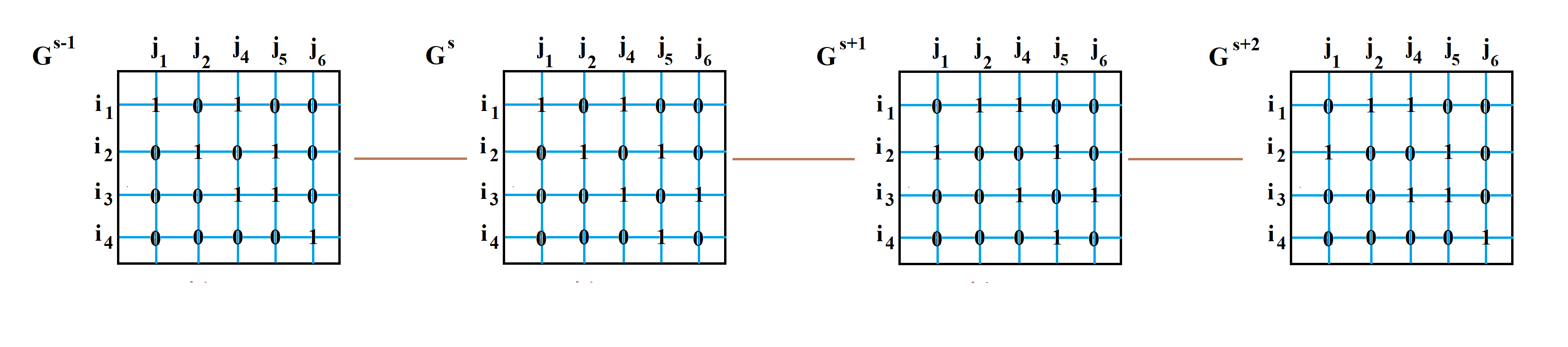
Figure 11. Proof of Lemma 6.10, Subcase 1d.

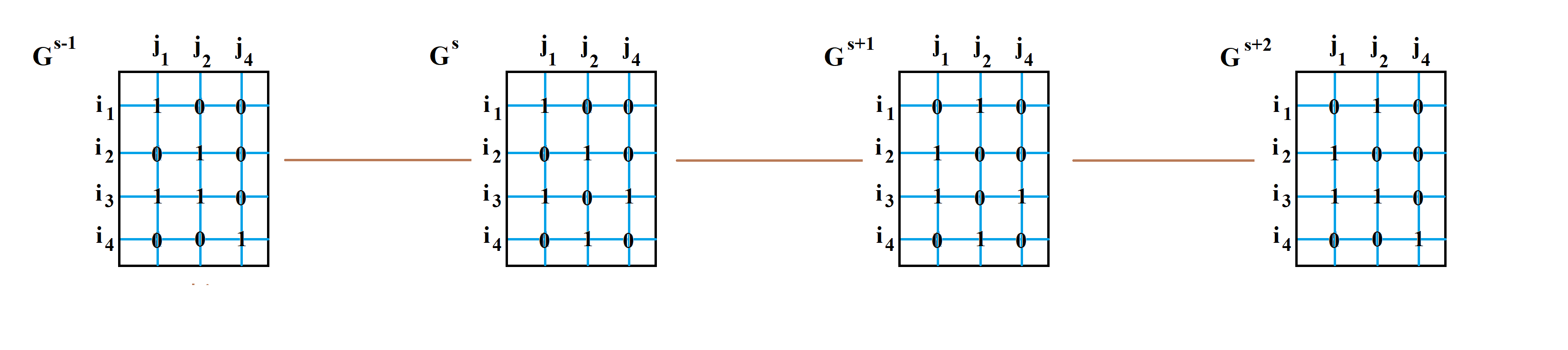
Figure 12. Proof of Lemma 6.10, Subcase 1e.

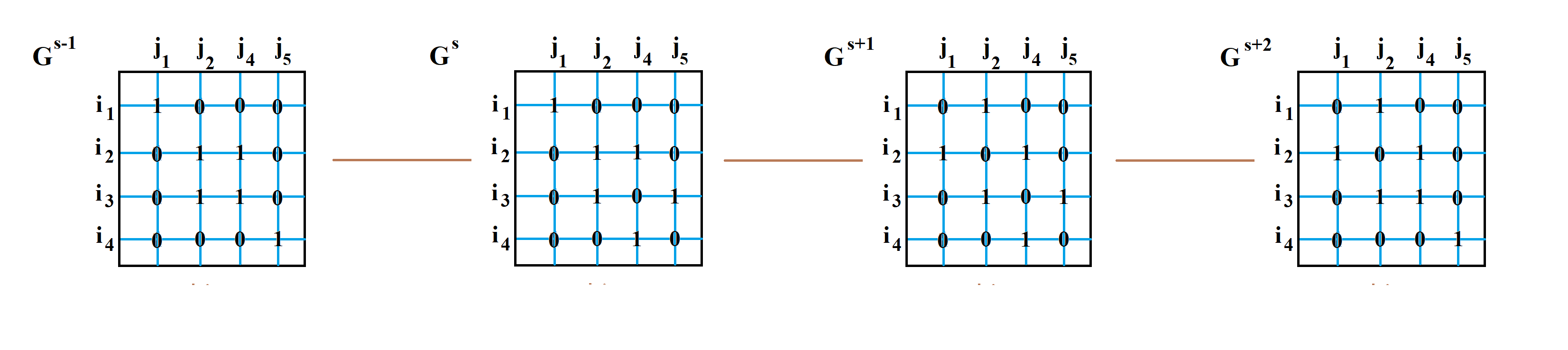
Figure 13. Proof of Lemma 6.10, an illustration to Subcase 1f.

Now, we are in position to construct a canonical path between the simple graphs. Let ${\mathcal{T}}=(G_{1},G_{1}^{\prime},G_{2},G_{2}^{\prime})$ be an admissible tuple.

Definition 6.11.

A connection (with respect to ${\mathcal{T}}$) is a path $P\subset\Omega^{B}_{n}(d)$ starting at $G_{1}$ and ending at $G_{2}$ constructed as follows:

• We set $P[0]:=G_{1}$.

• For each integer $1\leq t\leq 2|E_{S}({\mathcal{T}})|$, the simple graph $P[t]$ is obtained from $P[t-1]$ as follows. Let $i$ be the $\lceil t/2\rceil$–th smallest index with $(i,j)\in E_{S}({\mathcal{T}})$ for some $j$. Denote $i_{1}:={\bf i1}(i,{\mathcal{T}})$, $i_{2}:={\bf i2}(i,{\mathcal{T}})$, $j_{1}:={\bf j1}(i,{\mathcal{T}})$, $j_{2}:={\bf j2}(i,{\mathcal{T}})$. Then, if $t$ is odd, $P[t]$ is obtained by switching the edges $(i_{1},j)$ and $(i_{2},j_{2})$ of $P[t-1]$. Otherwise, if $t$ is even, $P[t]$ is obtained from $P[t-1]$ by switching the edges $(i_{1},j_{2})$ and $(i,j_{1})$ (see Figure 6). Once $P[2|E_{S}({\mathcal{T}})|]$ is constructed, set $t_{0}:=2|E_{S}({\mathcal{T}})|$ and go to the next stage of the construction.

• If $G_{1}^{\prime}$ and $G_{2}^{\prime}$ are adjacent and the switching transforming $G_{1}^{\prime}$ into $G_{2}^{\prime}$ (say, performed on edges $(v,w)$ and $(\tilde{v},\tilde{w})$) is of type A, we define $P[2|E_{S}({\mathcal{T}})|+1]$ by performing a simple switching on the edges $(v,w)$ and $(\tilde{v},\tilde{w})$ of $P[2|E_{S}({\mathcal{T}})|]$, and set $t_{0}:=2|E_{S}({\mathcal{T}})|+1$.

• If $I_{NS}({\mathcal{T}})$ is empty, the above construction gives the graph $G_{2}=P[t_{0}]$. Otherwise, if $I_{NS}({\mathcal{T}})$ is non-empty, we produce $G_{2}$ from $P[t_{0}]$ as follows. First, take the canonical partition $W_{1}\sqcup W_{2}\sqcup\dots\sqcup W_{h}$ of $I_{NS}({\mathcal{T}})$, set $G^{(0)}:=P[t_{0}]$, and for each $1\leq u\leq h$ let $G^{(u)}$ be the graph on $[n]\sqcup[n]$ whose adjacency matrix satisfies ${\rm row}_{i}({\rm Adj}(G^{(u)}))={\rm row}_{i}({\rm Adj}(G^{(u-1)}))$, $i\in[n]\setminus W_{u}$, and ${\rm row}_{i}({\rm Adj}(G^{(u)}))={\rm row}_{i}({\rm Adj}(G_{2}))$, $i\in W_{u}$. For each $u\leq h$, we apply

  • in the case when $|W_{u}|\in\{2,3,4\}$ — Lemma 6.9;

  • in the case $|W_{u}|\geq 5$ and $W_{u}$ comprises type B switching between $G_{1}^{\prime}$ and $G_{2}^{\prime}$ — Lemma 6.9;

  • in the case $|W_{u}|\geq 5$ and $W_{u}$ does not comprise type B switching — Lemma 6.10

  to subgraphs $G^{(u-1)}[W_{u}\sqcup[n]]$ and $G^{(u)}[W_{u}\sqcup[n]]$ to construct a path $\tilde{P}^{(u)}$ connecting $G^{(u-1)}$ and $G^{(u)}$ and satisfying all the properties listed in the lemmas. Then we complete the construction of $P$ by sequentially connecting $P[t_{0}]$ with $G^{(1)}$, $G^{(2)},\dots$, $G^{(h)}=G_{2}$ using the paths $\tilde{P}^{(u)}$.

It can be shown that the construction described above is valid, i.e. the prescribed simple switching operations at each stage can be performed, and that the ending vertex of $P$ is indeed $G_{2}$. In particular, in the case when $|W_{u}|\geq 5$ and $W_{u}$ does not comprise type B switching, the above subgraphs $G^{(u-1)}[W_{u}\sqcup[n]]$ and $G^{(u)}[W_{u}\sqcup[n]]$ do satisfy the conditions of Lemma 6.10:

Lemma 6.12.

Let $G^{(u-1)},G^{(u)}$ be graphs from the construction procedure above (for some $u$), and assume that $|W_{u}|\geq 5$ and $W_{u}$ does not comprise type B switching. Then the graphs $\tilde{G}_{1}:=G^{(u-1)}[W_{u}\sqcup[n]]$ and $\tilde{G}_{2}:=G^{(u)}[W_{u}\sqcup[n]]$ satisfy conditions of Lemma 6.10 with $k\leq 4|W_{u}|$.

Proof.

Obviously, both $\tilde{G}_{1}$ and $\tilde{G}_{2}$ have the same right degrees sequences because for every switching within the connection from $G_{1}$ to $G_{2}$, either both of the left vertices it operates on are contained in $W_{u}$ or none. The condition on $k$ comes from the next simple observation: any left vertex in $W_{u}$ can be used by at most one simple switching within the simple path from $G_{1}^{\prime}$ to $G_{1}$, and by at most one switching within the simple path from $G_{2}^{\prime}$ to $G_{2}$. Thus, within the corresponding rows of the adjacency matrices of $\tilde{G}_{1}$ and $\tilde{G}_{2}$, at most four elements can differ.

It remains to check the crucial condition on existence of common neighbors. The assumption that $|W_{u}|\geq 5$, implies that there are at least two distinct left vertices $v^{\prime},v^{\prime\prime}\in W_{u}$ and right vertices $z^{\prime},z^{\prime\prime}$ such that $(v^{\prime},z^{\prime})$ and $(v^{\prime\prime},z^{\prime\prime})$ are both multiedges in $G_{1}^{\prime}$. Further, by the definition of a simple path, the corresponding simple switching operations $\langle v^{\prime},g_{1}^{\prime},z^{\prime},x_{1}^{\prime}\rangle$ and $\langle v^{\prime\prime},g_{1}^{\prime\prime},z^{\prime\prime},x_{1}^{\prime\prime}\rangle$ within the simple path leading from $G_{1}^{\prime}$ to $G_{1}$, must satisfy $g_{1}^{\prime}\neq g_{1}^{\prime\prime}$ and $g_{1}^{\prime},g_{1}^{\prime\prime}\notin\{v^{\prime},v^{\prime\prime}\}$. In particular, $v^{\prime}$ must have a common neighbor with $W_{u}\setminus\{v^{\prime},v^{\prime\prime}\}$ and $v^{\prime\prime}$ must have a common neighbor with $W_{u}\setminus\{v^{\prime\prime}\}$ in graph $G_{1}$, hence in graph $\tilde{G}_{1}$. The same argument works for $\tilde{G}_{2}$. ∎

The main steps of the construction procedure are reflected in Figure 14.

Note that the path described above may not be uniquely defined whenever $I_{NS}({\mathcal{T}})$ is non-empty (because Lemmas 6.9 and 6.10 confirm existence but not uniqueness of respective subpaths). In this case we fix any admissible path for the given $4$–tuple ${\mathcal{T}}$ satisfying the above conditions. Often, to emphasize dependence on the $4$–tuple, we will denote the connection for ${\mathcal{T}}$ by $P_{\mathcal{T}}$.

Remark 6.13.

The length of $P_{\mathcal{T}}$ is always at least $2|E_{S}({\mathcal{T}})|$, and is equal to $2|E_{S}({\mathcal{T}})|$ when $G_{1}^{\prime}=G_{2}^{\prime}$ and $I_{NS}({\mathcal{T}})$ is empty. In general, the length of $P_{\mathcal{T}}$ can be bounded from above by $2|E_{S}({\mathcal{T}})|+C_{\text{\tiny\ref{l: 2095203598305298 bis}}}(8|I_{NS}({\mathcal{T}})|+4)$, in view of Lemmas 6.9, 6.10, and 6.5.

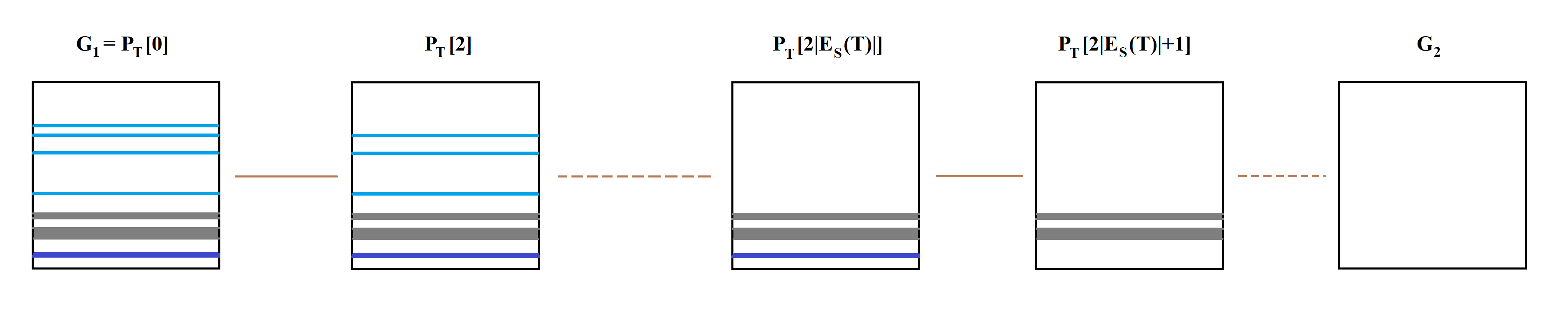
Figure 14. A schematic depiction of a connection for a tuple ${\mathcal{T}}=(G_{1},G_{1}^{\prime},G_{2},G_{2}^{\prime})$ in the case when the graphs $G_{1}^{\prime}$ and $G_{2}^{\prime}$ are connected by a type $A$ switching. The graphs are represented by their adjacency matrices. The first $2|E_{S}({\mathcal{T}})|$ steps of the connection deal with rows associated with $m$–standard edges (shown in light blue). The graphs $P_{\mathcal{T}}[2|E_{S}({\mathcal{T}})|]$ and $P_{\mathcal{T}}[2|E_{S}({\mathcal{T}})|+1]$ are related by a switching of type $A$ (corresponding couple of rows is colored in dark blue and are shown as “adjacent” for simplicity). The last ${\rm len}(P_{\mathcal{T}})-2|E_{S}({\mathcal{T}})|-1$ steps deal with the set $I_{NS}({\mathcal{T}})$ which is in turn represented via the canonical partition (grey). The uncolored rows of adjacency matrices coincide with those of $G_{2}$.

Definition 6.14.

For each $t\leq{\rm len}(P_{\mathcal{T}})$, we say that the couple $(P_{\mathcal{T}}[t-1],P_{\mathcal{T}}[t])$ is

• $m$–standard if $t\leq 2|E_{S}({\mathcal{T}})|$;

• of type A if $G_{1}^{\prime}$ and $G_{2}^{\prime}$ are connected by a type $A$ switching, and that is the simple switching operation taking $P_{\mathcal{T}}[t-1]$ to $P_{\mathcal{T}}[t]$ (note that necessarily $t=2|E_{S}({\mathcal{T}})|+1$ in this case);

• $NS$–couple if the left vertices participating in the switching from $P_{\mathcal{T}}[t-1]$ to $P_{\mathcal{T}}[t]$, belong to $I_{NS}({\mathcal{T}})$.

6.3. Complexity of $I_{NS}({\mathcal{T}})$

The goal of this subsection is to count the number of possible distinct realizations of the set $I_{NS}({\mathcal{T}})$ such that the corresponding connection $P_{\mathcal{T}}$ contains a given pair of adjacent simple graphs $(\Gamma,\tilde{\Gamma})$. This estimate will then be used to bound the total number of tuples ${\mathcal{T}}$ with $P_{\mathcal{T}}$ containing the couple $(\Gamma,\tilde{\Gamma})$. We start with two auxiliary lemmas.

Lemma 6.15.

Let ${\mathcal{T}}=(G_{1},G_{1}^{\prime},G_{2},G_{2}^{\prime})$ be an admissible $4$–tuple, and let $W_{q}\neq\emptyset$ be the $q$–th element of the canonical partition of $I_{NS}({\mathcal{T}})$. Then necessarily there is a right vertex $j\in[n]$ having at least two neighbors in $W_{q}$ in each of the graphs $G_{1}$ and $G_{2}$.

Proof.

Note that, by the definition of the canonical partition, the path $P$ from $G_{1}$ to $G_{2}$ in ${\mathcal{M}}^{B}_{n}(d)$ obtained by concatenation of simple paths from $G_{1}^{\prime}$ to $G_{1}$ and $G_{2}^{\prime}$ to $G_{2}$, and of the simple switching connecting $G_{1}^{\prime}$ and $G_{2}^{\prime}$ (if any), has the property that for any $t\leq{\rm len}(P)$, the simple switching from $P[t-1]$ to $P[t]$ operates on left vertices which either are both contained in $W_{q}$ or are both not contained in $W_{q}$. Thus, necessarily $G_{1}[W_{q}\sqcup[n]]$ has the same right degrees sequence as $G_{2}[W_{q}\sqcup[n]]$, so it is enough to check the statement for one of the graphs $G_{1}$ or $G_{2}$. But then the result follows immediately since each $W_{q}$ must contain at least one left vertex incident to a multiedge either in $G_{1}^{\prime}$ or $G_{2}^{\prime}$, so the corresponding right vertex $j$ has the required properties. ∎

Lemma 6.16.

Let ${\mathcal{T}}=(G_{1},G_{1}^{\prime},G_{2},G_{2}^{\prime})$ be admissible, and let $t\geq 1$ be such that $(P_{\mathcal{T}}[t-1],P_{\mathcal{T}}[t])$ is $NS$–couple in $P_{\mathcal{T}}$. Let $W_{q}=W_{q}({\mathcal{T}})$ be the element of the canonical partition of $I_{NS}({\mathcal{T}})$ which contains left vertices $\{i_{1},i_{2}\}$ operated on by the simple switching leading from $P_{\mathcal{T}}[t-1]$ to $P_{\mathcal{T}}[t]$, and assume that $|W_{q}|\geq 3$. Then necessarily there is a left vertex $i_{3}\in W_{q}\setminus\{i_{1},i_{2}\}$ which has a common neighbor with $W_{q}\setminus\{i_{3}\}$ in $P_{\mathcal{T}}[t-1]$.

Proof.

By the definition of a connection, the part of the path $P_{\mathcal{T}}$ which transforms the subgraph of $G_{1}$ on $W_{q}\sqcup[n]$ into the respective subgraph of $G_{2}$, satisfies all the conditions listed in Lemma 6.9 or 6.10. Specifically, at least one of the following must be true:

• $i_{1}$ and $i_{2}$ have no common neighbors in $P_{\mathcal{T}}[t-1]$;

• there is a left vertex $i_{3}\in W_{q}\setminus\{i_{1},i_{2}\}$ having at least one common neighbor with $W_{q}\setminus\{i_{3}\}$ in $P_{\mathcal{T}}[t-1]$.

Note that, in view of Lemma 6.15, there is a right vertex $j$ having at least two neighbors in $W_{q}$ in both graphs $G_{1}$ and $G_{2}$, hence in graphs $P_{\mathcal{T}}[t-1]$ and $P_{\mathcal{T}}[t]$ as well.

In the first case, since $i_{1}$ and $i_{2}$ have no common neighbors, $j$ must be adjacent to at least one left vertex $i_{3}\notin\{i_{1},i_{2}\}$. This left vertex satisfies the necessary conditions.

In the second case we have the required property automatically. The result follows. ∎

In the following three lemmas, we consider the problem of estimating the number of possible realizations for a given element of the canonical partition of $I_{NS}({\mathcal{T}})$.

In the first two lemmas, we study the complexity of the sets $W_{q}({\mathcal{T}})$ under the assumption that the switching connecting $\Gamma$ and $\tilde{\Gamma}$ is not “contained” in $W_{q}({\mathcal{T}})$.

Lemma 6.17.

Let $(\Gamma,\tilde{\Gamma})$ be a pair of adjacent graphs in $\Omega^{B}_{n}(d)$, and $q,r_{q}\in{\mathbb{N}}$. Let $T$ be the collection of all admissible $4$–tuples ${\mathcal{T}}=(G_{1},G_{1}^{\prime},G_{2},G_{2}^{\prime})$ such that

• $P_{\mathcal{T}}$ contains the pair $(\Gamma,\tilde{\Gamma})$, and

• the left vertices operated on by the simple switching leading from $\Gamma$ to $\tilde{\Gamma}$ do not belong to $W_{q}({\mathcal{T}})$, and

• $|W_{q}({\mathcal{T}})|=r_{q}$, and

• $G_{1}^{\prime}=G_{2}^{\prime}$ or the simple switching leading from $G_{1}^{\prime}$ to $G_{2}^{\prime}$ operates on left vertices that do not belong to $W_{q}({\mathcal{T}})$.

Then the cardinality of the set

$${\bf W}:=\big{\{}W\subset[n]:\;\mbox{$W=W_{q}({\mathcal{T}})$ for some ${\mathcal{T}}\in T$}\big{\}}$$

is bounded above by $4n^{\max(1,r_{q}-2)}\big{(}\max(1,r_{q}-2)d(d-1)\big{)}^{2}$.

Proof.

Note that, by the conditions on the couple $(\Gamma,\tilde{\Gamma})$, for every ${\mathcal{T}}\in T$, either

$$\Gamma[W_{q}({\mathcal{T}})\sqcup[n]]=\tilde{\Gamma}[W_{q}({\mathcal{T}})\sqcup[n]]=G_{1}[W_{q}({\mathcal{T}})\sqcup[n]]$$

or

$$\Gamma[W_{q}({\mathcal{T}})\sqcup[n]]=\tilde{\Gamma}[W_{q}({\mathcal{T}})\sqcup[n]]=G_{2}[W_{q}({\mathcal{T}})\sqcup[n]].$$

Denote the subset of $T$ of tuples satisfying the former condition by $T_{1}$, and the latter condition — by $T_{2}$.

For any ${\mathcal{T}}\in T$, denote by $M_{q}({\mathcal{T}})$ the number of multiedges of $G_{h}^{\prime}$ incident to $W_{q}({\mathcal{T}})$, $h=1,2$ (observe that the quantity is the same for both graphs $G_{1}^{\prime}$ and $G_{2}^{\prime}$). Denote by $T^{\prime}$ the subset of all ${\mathcal{T}}\in T$ with $M_{q}({\mathcal{T}})>1$.

Now, let us consider several cases:

• Treatment of $T^{\prime}\cap T_{1}$. For any ${\mathcal{T}}\in T^{\prime}\cap T_{1}$ we observe that, in view of the definition of a simple path and sets $T^{\prime},T_{1}$, $W_{q}({\mathcal{T}})$ contains at least two left vertices from $I_{s}(G_{1},G_{1}^{\prime})$ which have common neighbors with $W_{q}({\mathcal{T}})\cap I_{m}(G_{1},G_{1}^{\prime})$ in $\Gamma$. Thus, the set $W_{q}({\mathcal{T}})$ for ${\mathcal{T}}\in T^{\prime}\cap T_{1}$ can be determined first by choosing $r_{q}-2$ left vertices from $[n]$ and then choosing two more vertices having common neighbors with the given $(r_{q}-2)$–set. Clearly, the number of choices for the latter is bounded above by $((r_{q}-2)d(d-1))^{2}$, whence

  $$\big{|}\big{\{}W_{q}({\mathcal{T}}):\;{\mathcal{T}}\in T^{\prime}\cap T_{1}\big{\}}\big{|}\leq n^{r_{q}-2}((r_{q}-2)d(d-1))^{2}.$$

• Treatment of $T^{\prime}\cap T_{2}$. Similarly, we get

  $$\big{|}\big{\{}W_{q}({\mathcal{T}}):\;{\mathcal{T}}\in T^{\prime}\cap T_{2}\big{\}}\big{|}\leq n^{r_{q}-2}((r_{q}-2)d(d-1))^{2}.$$

• Treatment of $T\setminus T^{\prime}$. Now, consider the case when ${\mathcal{T}}\in T\setminus T^{\prime}$. Note that in this case the set $W_{q}({\mathcal{T}})$ can have cardinality either $2$ or $3$. In the former case, we necessarily have $W_{q}({\mathcal{T}})\cap I_{s}(G_{1},G_{1}^{\prime})=W_{q}({\mathcal{T}})\cap I_{s}(G_{2},G_{2}^{\prime})$, and the unique left vertex contained in this set must have at least one common neighbor with $W_{q}({\mathcal{T}})\cap I_{m}(G_{1},G_{1}^{\prime})=W_{q}({\mathcal{T}})\cap I_{m}(G_{2},G_{2}^{\prime})$.

  In the latter case, the only reason why the multiedge of $G_{1}^{\prime}$ (and $G_{2}^{\prime}$) incident to $W_{q}({\mathcal{T}})\cap I_{m}(G_{1},G_{1}^{\prime})=W_{q}({\mathcal{T}})\cap I_{m}(G_{2},G_{2}^{\prime})$ is not $m$–standard is a violation of property (4) in the definition of $m$–standard edges. It is not difficult to see that without this property, there must exist a left vertex $i\in W_{q}({\mathcal{T}})$ having common neighbors with both remaining vertices of $W_{q}({\mathcal{T}})\setminus\{i\}$ in $\Gamma$ (see Figures 7).

  Taking into account these observations we obtain that

  $$\big{|}\big{\{}W_{q}({\mathcal{T}}):\;{\mathcal{T}}\in T\setminus T^{\prime}\big{\}}\big{|}\leq nd(d-1)+nd(d-1)^{3}\leq 2n(d(d-1))^{2}.$$

The result follows by combining the estimates. ∎

Lemma 6.18.

Let $(\Gamma,\tilde{\Gamma})$ be a pair of adjacent graphs in $\Omega^{B}_{n}(d)$, and $q,r_{q}\in{\mathbb{N}}$. Let $T$ be the collection of all admissible $4$–tuples ${\mathcal{T}}=(G_{1},G_{1}^{\prime},G_{2},G_{2}^{\prime})$ such that

• $P_{\mathcal{T}}$ contains the pair $(\Gamma,\tilde{\Gamma})$, and

• the left vertices operated on by the simple switching leading from $\Gamma$ to $\tilde{\Gamma}$ are not contained in $W_{q}({\mathcal{T}})$, and

• $|W_{q}({\mathcal{T}})|=r_{q}$, and

• the simple switching leading from $G_{1}^{\prime}$ to $G_{2}^{\prime}$ operates on left vertices contained in $W_{q}({\mathcal{T}})$.

Then the cardinality of the set

$${\bf W}:=\big{\{}W\subset[n]:\;\mbox{$W=W_{q}({\mathcal{T}})$ for some ${\mathcal{T}}\in T$}\big{\}}$$

is bounded above by $n^{r_{q}-1}(r_{q}-1)d(d-1)$.

Proof.

Applying Lemma 6.15, we immediately get that for any ${\mathcal{T}}=(G_{1},G_{1}^{\prime},G_{2},G_{2}^{\prime})\in T$, there is right vertex $j=j({\mathcal{T}})$ which has at least two neighbors in $W_{q}({\mathcal{T}})$ in each of the two graphs $G_{1}$, $G_{2}$, hence in graphs $\Gamma$ and $\tilde{\Gamma}$ as well. Thus, each set from ${\bf W}$ can be identified first by choosing $(r_{q}-1)$–subset of $[n]$ and then choosing a left vertex having at least one common neighbor with the given subset. Thus,

$$|{\bf W}|\leq n^{r_{q}-1}(r_{q}-1)d(d-1).$$

∎

Now, we consider the situation when the simple switching connecting $\Gamma$ and $\tilde{\Gamma}$ is “contained” in $W_{q}({\mathcal{T}})$.

Lemma 6.19.

Let $(\Gamma,\tilde{\Gamma})$ be a pair of adjacent graphs in $\Omega^{B}_{n}(d)$, and $q,r_{q}\in{\mathbb{N}}$. Let $T$ be the collection of all admissible $4$–tuples ${\mathcal{T}}=(G_{1},G_{1}^{\prime},G_{2},G_{2}^{\prime})$ such that

• $(\Gamma,\tilde{\Gamma})$ is a $NS$–couple in the connection $P_{\mathcal{T}}$, and

• the left vertices operated on by the simple switching leading from $\Gamma$ to $\tilde{\Gamma}$ are contained in $W_{q}({\mathcal{T}})$, and

• $|W_{q}({\mathcal{T}})|=r_{q}$.

Then the cardinality of the set

$${\bf W}:=\big{\{}W\subset[n]:\;\mbox{$W=W_{q}({\mathcal{T}})$ for some ${\mathcal{T}}\in T$}\big{\}}$$

is bounded above by $\max\big{(}1,n^{r_{q}-3}(r_{q}-1)d(d-1)\big{)}$.

Furthermore, assume that $r_{q}\geq 5$, and denote by $T^{\prime}$ the subset of tuples ${\mathcal{T}}=(G_{1},G_{1}^{\prime},G_{2},G_{2}^{\prime})\in T$ such that either $G_{1}^{\prime}=G_{2}^{\prime}$ or the switching connecting $G_{1}^{\prime}$ and $G_{2}^{\prime}$ does not operate on vertices in $W_{q}({\mathcal{T}})$. Then the cardinality of the set

$${\bf W^{\prime}}:=\big{\{}W\subset[n]:\;\mbox{$W=W_{q}({\mathcal{T}})$ for some ${\mathcal{T}}\in T^{\prime}$}\big{\}}$$

can be bounded above by $n^{r_{q}-4}(r_{q}-1)(r_{q}-2)d^{2}(d-1)^{2}$.

Proof.

When $r_{q}=2$, the above bound for $|{\bf W}|$ is obvious, so we shall consider the case when $r_{q}\geq 3$. Let $\{i_{1},i_{2}\}$ be the pair of left vertices operated on by the simple switching transforming $\Gamma$ to $\tilde{\Gamma}$. Applying Lemma 6.16, we get that any subset $W\in{\bf W}$ must contain at least one left vertex $i$ (distinct from $i_{1},i_{2}$) which has common neighbors with $W\setminus\{i\}$. Hence, any set $W\in{\bf W}$ can be identified by first picking $(r_{q}-3)$–subset of $[n]\setminus\{i_{1},i_{2}\}$ and then selecting a left vertex having at least one common neighbor with either the constructed $(r_{q}-3)$–subset or $\{i_{1},i_{2}\}$. The $d$–regularity implies that the number of choices for this last index is at most $(r_{q}-1)d(d-1)$, and the first bound follows.

Now, consider the case $r_{q}\geq 5$. Note that in this case the total multiplicity of multiedges of each of the graphs $G_{1}^{\prime},G_{2}^{\prime}$ incident to $W_{q}({\mathcal{T}})$ must be at least four, and the part of the connection is constructed according to Lemma 6.10. Hence, we get that for each tuple ${\mathcal{T}}\in T^{\prime}$ there are two left vertices $\{i^{\prime},i^{\prime\prime}\}\subset W_{q}({\mathcal{T}})$ disjoint from the vertices operated on by the switching connecting $\Gamma$ and $\tilde{\Gamma}$, such that $i^{\prime}$ has a common neighbor with $W_{q}({\mathcal{T}})\setminus\{i^{\prime}\}$ in $\Gamma$ and $i^{\prime\prime}$ has a common neighbor with $W_{q}({\mathcal{T}})\setminus\{i^{\prime},i^{\prime\prime}\}$. Hence, a set $W\in{\bf W^{\prime}}$ can be identified by first picking $(r_{q}-4)$–subset of $[n]\setminus\{i_{1},i_{2}\}$, then selecting a left vertex having at least one common neighbor with either the constructed $(r_{q}-4)$–subset or $\{i_{1},i_{2}\}$, and finally picking one more left vertex having at least one common neighbor with the $(r_{q}-1)$–subset. The total number of choices can be bounded above by $n^{r_{q}-4}(r_{q}-2)d(d-1)(r_{q}-1)d(d-1)$. The result follows. ∎

Finally, we are in position to compute “complexity” of $I_{NS}({\mathcal{T}})$ by combining the above three lemmas. Let us introduce additional classification on the set of admissible $4$–tuples of graphs.

Definition 6.20.

Let $k_{1},k_{2},r\in{\mathbb{N}}$ and $u\in\{A,B\}$. We say that a $4$–tuple ${\mathcal{T}}=(G_{1},G_{1}^{\prime},G_{2},G_{2}^{\prime})$ is of subtype $1$–$(k_{1},k_{2},u,r)$ if all of the following conditions are satisfied:

• ${\mathcal{T}}$ is of type $1$;

• $G_{1}^{\prime}$ is of category $k_{1}$ and $G_{2}^{\prime}$ is of category $k_{2}$;

• $|I_{NS}({\mathcal{T}})|=r$;

• $G_{1}^{\prime}$ and $G_{2}^{\prime}$ are adjacent, and the simple switching operation transforming $G_{1}^{\prime}$ to $G_{2}^{\prime}$ is of type $u$.

Similarly,

Definition 6.21.

We say that an admissible $4$–tuple ${\mathcal{T}}=(G_{1},G^{\prime},G_{2},G^{\prime})$ is of subtype $2$–$(k,r)$, $k,r\in{\mathbb{N}}$, if

• $G_{1},G_{2}\in{\mathcal{S}\mathcal{N}}(G^{\prime})$;

• $G^{\prime}$ is of category $k$;

• $|I_{NS}({\mathcal{T}})|=r$.

For the reader’s convenience, we group together the classification of $4$–tuples used in this section in the following table.

Type	Subtype /  Remarks
Type $1$ tuples. Tuples $(G_{1},G_{1}^{\prime},G_{2},G_{2}^{\prime})$ such that $G_{1}\in{\mathcal{S}\mathcal{N}}(G_{1}^{\prime})$, $G_{2}\in{\mathcal{S}\mathcal{N}}(G_{2}^{\prime})$, the graphs $G_{1}^{\prime}$ and $G_{2}^{\prime}$ are adjacent in ${\mathcal{M}}^{B}_{n}(d)$; $G_{1}^{\prime},G_{2}^{\prime}\in{\rm Cat}_{n,d}([1,{\mathfrak{m}}])$, and the pair $(G_{1}^{\prime},G_{2}^{\prime})$ is not perfect.	Subtype $1$–$(k_{1},k_{2},A,r)$. $G_{1}^{\prime}$ has category $k_{1}$, $G_{2}^{\prime}$ — category $k_{2}$, $|I_{NS}({\mathcal{T}})|=r$, and $G_{1}^{\prime}$ and $G_{2}^{\prime}$ are connected by a type $A$ switching.
	Subtype $1$–$(k_{1},k_{2},B,r)$. $G_{1}^{\prime}$ has category $k_{1}$, $G_{2}^{\prime}$ — category $k_{2}$, $|I_{NS}({\mathcal{T}})|=r$, and $G_{1}^{\prime}$ and $G_{2}^{\prime}$ are connected by a type $B$ switching.
Type $2$ tuples. Tuples $(G_{1},G^{\prime},G_{2},G^{\prime})$ such that $G_{1}\in{\mathcal{S}\mathcal{N}}(G^{\prime})$, $G_{2}\in{\mathcal{S}\mathcal{N}}(G^{\prime})$, and $G^{\prime}\in{\rm Cat}_{n,d}([1,{\mathfrak{m}}])$.	Subtype $2$–$(k,r)$. $G^{\prime}$ has category $k$, and $|I_{NS}({\mathcal{T}})|=r$.
Type $3$ tuples. Tuples $(G_{1},G_{1},G_{2},G_{2}^{\prime})$ such that $G_{1}\in\Omega^{B}_{n}(d)$ is adjacent to $G_{2}^{\prime}\in{\rm Cat}_{n,d}([1,{\mathfrak{m}}])$, and $G_{2}\in{\mathcal{S}\mathcal{N}}(G_{2}^{\prime})$, $G_{1}\notin{\mathcal{S}\mathcal{N}}(G_{2}^{\prime})$.	For every type $3$ tuple, the category of $G_{2}^{\prime}$ is equal to $2$, and $G_{1}$ and $G_{2}^{\prime}$ are connected by a type $B$ switching.

Proposition 6.22 (Complexity of $I_{NS}({\mathcal{T}})$).

Let $(\Gamma,\tilde{\Gamma})$ be a pair of adjacent graphs in $\Omega^{B}_{n}(d)$, and let $k_{1},k_{2}\in{\mathbb{N}}$, $r\geq 1$, $N_{ms}\geq 0$. Then

1. The number of distinct realizations of $I_{NS}({\mathcal{T}})$ over all $4$–tuples ${\mathcal{T}}=(G_{1},G_{1}^{\prime},G_{2},G_{2}^{\prime})$ of subtype $1$–$(k_{1},k_{2},A,r)$ such that $|E_{S}({\mathcal{T}})|=N_{ms}$ and $(\Gamma,\tilde{\Gamma})$ is an $m$–standard couple or an $A$–couple in $P_{\mathcal{T}}$, is bounded above by

   $$8^{r}n^{k_{1}+k_{2}-2N_{ms}-1}\big{(}rd(d-1)\big{)}^{r}.$$

   Similarly, the number of distinct realizations of $I_{NS}({\mathcal{T}})$ over tuples ${\mathcal{T}}=(G_{1},G^{\prime},G_{2},G^{\prime})$ of subtype $2$–$(k_{1},r)$ such that $|E_{S}({\mathcal{T}})|=N_{ms}$ and $(\Gamma,\tilde{\Gamma})$ is an $m$–standard couple in $P_{\mathcal{T}}$, is bounded above by

   $$8^{r}n^{2k_{1}-2N_{ms}-1}\big{(}rd(d-1)\big{)}^{r}.$$

2. The number of distinct realizations of $I_{NS}({\mathcal{T}})$ over all $4$–tuples ${\mathcal{T}}=(G_{1},G_{1}^{\prime},G_{2},G_{2}^{\prime})$ of subtype $1$–$(k_{1},k_{2},B,r)$ such that $|E_{S}({\mathcal{T}})|=N_{ms}$ and $(\Gamma,\tilde{\Gamma})$ is an $m$–standard couple in $P_{\mathcal{T}}$, is bounded above by

   $$8^{r}\,r\,n^{k_{1}+k_{2}-2N_{ms}+1}\big{(}rd(d-1)\big{)}^{r}.$$

3. The number of distinct realizations of $I_{NS}({\mathcal{T}})$ over all $4$–tuples ${\mathcal{T}}=(G_{1},G_{1}^{\prime},G_{2},G_{2}^{\prime})$ of subtype $1$–$(k_{1},k_{2},A,r)$ such that $|E_{S}({\mathcal{T}})|=N_{ms}$ and $(\Gamma,\tilde{\Gamma})$ is an $NS$–couple in $P_{\mathcal{T}}$, is bounded above by

   $$(r-1)d(d-1),\quad\mbox{ if $r\leq 3$},$$

   and

   $$8^{r}\,r\,n^{k_{1}+k_{2}-2N_{ms}-3}\big{(}rd(d-1)\big{)}^{r},\quad\mbox{ if $r\geq 4$}.$$

   Similarly, the number of distinct realizations of $I_{NS}({\mathcal{T}})$ over tuples ${\mathcal{T}}=(G_{1},G^{\prime},G_{2},G^{\prime})$ of subtype $2$–$(k_{1},r)$ such that $|E_{S}({\mathcal{T}})|=N_{ms}$ and $(\Gamma,\tilde{\Gamma})$ is an $NS$–couple in $P_{\mathcal{T}}$, is bounded above by $(r-1)d(d-1)$ for $r\leq 3$ and by $8^{r}\,r\,n^{2k_{1}-2N_{ms}-3}\big{(}rd(d-1)\big{)}^{r}$ for $r\geq 4$.

4. The number of distinct realizations of $I_{NS}({\mathcal{T}})$ over all $4$–tuples ${\mathcal{T}}=(G_{1},G_{1}^{\prime},G_{2},G_{2}^{\prime})$ of subtype $1$–$(k_{1},k_{2},B,r)$ such that $|E_{S}({\mathcal{T}})|=N_{ms}$ and $(\Gamma,\tilde{\Gamma})$ is an $NS$–couple in $P_{\mathcal{T}}$, is bounded above by

   $$8^{r}\,r^{2}\,n^{k_{1}+k_{2}-2N_{ms}-1}\big{(}rd(d-1)\big{)}^{r}.$$

Proof.

1. Fix any sequence of non-negative integers $(r_{1},r_{2},\dots)$, such that $r_{q}=0$ implies $r_{q+1}=0$ for all $q\geq 1$, and such that $\sum_{q=1}^{\infty}r_{q}=r$. First, we shall estimate the number of realizations of sets $I_{NS}({\mathcal{T}})$ whose canonical partitions $(W_{q}({\mathcal{T}}))_{q=1}^{\infty}$ satisfy $|W_{q}({\mathcal{T}})|=r_{q}$, $q\geq 1$. Applying Lemma 6.17, we get that the number of realizations of each non-empty $W_{q}$ is bounded above by $4n^{\max(1,r_{q}-2)}\big{(}\max(1,r_{q}-2)d(d-1)\big{)}^{2}$ (regardless whether we consider type $1$ or type $2$). Taking the product, we obtain that the number of realizations of $I_{NS}({\mathcal{T}})$ with the cardinalities of the elements of the canonical partition encoded by the sequence $(r_{q})_{q=1}^{\infty}$, is bounded above by

   $$4^{r}n^{\sum_{q\geq 1,\,r_{q}\neq 0}\max(1,r_{q}-2)}\big{(}rd(d-1)\big{)}^{r},$$

   where we have used that the number of non-zero elements of the sequence $(r_{q})$ is at most $r/2$. Observe that, in notation of Lemma 6.7,

   $$\sum_{q\geq 1,\,W_{q}({\mathcal{T}})\neq\emptyset}M^{h}_{q}=k_{h}-N_{ms},\quad h=1,2.$$

   Thus, in view of Lemma 6.7, for every ${\mathcal{T}}$ of subtype $1$–$(k_{1},k_{2},A,r)$ satisfying the conditions in the first part of the proposition we have

   $$\sum_{q\geq 1,\,W_{q}({\mathcal{T}})\neq\emptyset}\max(1,|W_{q}({\mathcal{T}})|-2)\leq k_{1}+k_{2}-2N_{ms}-1\quad\mbox{ whenever $r\neq 0$.}$$

   Similarly, for every ${\mathcal{T}}$ of subtype $2$–$(k_{1},r)$ satisfying the conditions in the first part of the proposition we have $\sum_{q\geq 1,\,W_{q}({\mathcal{T}})\neq\emptyset}\max(1,|W_{q}({\mathcal{T}})|-2)\leq 2k_{1}-2N_{ms}-1$, whenever $r\neq 0$. Further, the total number of admissible realizations of $(r_{1},r_{2},\dots)$ can be (roughly) bounded from above by $2^{r}$; thus the number of admissible realizations of $I_{NS}({\mathcal{T}})$ for type $1$ case is bounded from above by

   $$8^{r}n^{k_{1}+k_{2}-2N_{ms}-1}\big{(}rd(d-1)\big{)}^{r},$$

   with the straightforward modification for subtype $2$–$(k_{1},r)$ tuples.

2. As in the previous case, we fix a sequence of non-negative integers $(r_{1},r_{2},\dots)$, and, additionally, fix a number $u\leq r$ which will serve as a label for the element of the canonical partition containing the left vertices operated on by the simple switching connecting $G_{1}^{\prime}$ and $G_{2}^{\prime}$. Applying Lemma 6.17 and Lemma 6.18, we get that the total number of realizations of $I_{NS}({\mathcal{T}})$ satisfying $|W_{q}({\mathcal{T}})|=r_{q}$, $q\geq 1$, and $W_{u}({\mathcal{T}})$ containing the left vertices used to switch from $G_{1}^{\prime}$ to $G_{2}^{\prime}$, is bounded above by

   $$n^{r_{u}-1}(r_{u}-1)d(d-1)\prod\limits_{q\neq u,\,r_{q}\neq 0}\Big{(}4n^{\max(1,r_{q}-2)}\big{(}\max(1,r_{q}-2)d(d-1)\big{)}^{2}\Big{)}.$$

   Invoking Lemma 6.7 (the “in particular” part of the lemma, to be precise), we get that

   $$r_{u}+\sum_{q\neq u,\,r_{q}\neq 0}\max(1,r_{q}-2)\leq k_{1}+k_{2}-2N_{ms}+2$$

   (the worst-case estimate corresponds to the situation when $r_{u}=r_{1}=r$), whence the previous expression can be bounded from above by

   $$4^{r}\big{(}rd(d-1)\big{)}^{r}n^{k_{1}+k_{2}-2N_{ms}+1}.$$

   The result follows by summing over all possible choices of $(r_{q})_{q=1}^{\infty}$ and $u\leq r$.

3. Again, we fix a sequence $(r_{1},r_{2},\dots)$ with $\sum_{q=1}^{\infty}r_{q}=r$, and, additionally, fix a number $u\leq r$ which identifies the element of the canonical partition containing the left vertices $\{i_{1},i_{2}\}$ operated on by the simple switching connecting $\Gamma$ and $\tilde{\Gamma}$.

   First, consider the case $r\leq 3$. Note that in this case $I_{NS}({\mathcal{T}})$ consists of a single set $W_{1}$, which comprises exactly one multiedge. Applying Lemma 6.19, we get upper bound $(r-1)d(d-1)$ for the complexity, both for subtype $1$–$(k_{1},k_{2},A,r)$ tuples and for subtype $2$–$(k_{1},r)$ tuples.

   Now, assume that $r\geq 4$. We have to consider two subcases then.

   • There is $q\neq u$ with $r_{q}\neq 0$. Then, applying Lemmas 6.17 and 6.19 as above, we get that the number of possible realizations is bounded above by

     $$n^{\max(1,r_{u}-2)-1}(r_{u}-1)d(d-1)\cdot$$

     $$\prod\limits_{q\neq u,\,r_{q}\neq 0}\big{(}4n^{\max(1,r_{q}-2)}\big{(}\max(1,r_{q}-2)d(d-1)\big{)}^{2}\big{)}$$

     $$\leq 4^{r}\big{(}rd(d-1)\big{)}^{r}n^{k_{1}+k_{2}-2N_{ms}-3},$$

     where we also used Lemma 6.7 (the first assertion $\max(1,r_{x}-2)\leq 2M_{x}^{1}-1=2M_{x}^{2}-1$, to be precise), and this time took into account that there are factors corresponding to $q\neq u,\,r_{q}\neq 0$, with straightforward modification for subtype $2$–$(k_{1},r)$.

   • There is no $q\neq u$ with $r_{q}\neq 0$. Then necessarily $r_{u}\geq 4$. If $r_{u}=4$ then using Lemma 6.19 we bound the complexity by

     $$n^{r_{u}-3}(r_{u}-1)d(d-1)=3nd(d-1)\leq 3d(d-1)n^{k_{1}+k_{2}-2N_{ms}-3},$$

     where we use the simple observation that $k_{1}+k_{2}-2N_{ms}\geq 4$ under the assumption $r>3$. If $r_{u}\geq 5$ then we apply the “furthermore” part of Lemma 6.19 to get the upper bound

     $$n^{r_{u}-4}(r_{u}-1)(r_{u}-2)d^{2}(d-1)^{2}\leq r^{2}d^{2}(d-1)^{2}n^{k_{1}+k_{2}-2N_{ms}-3},$$

     where the last inequality follows by appying Lemma 6.7. Again, a direct modification of the argument gives $r^{2}d^{2}(d-1)^{2}n^{2k_{1}-2N_{ms}-3}$ as the upper bound in subtype $2$–$(k_{1},r)$ case.

   Summing over $(r_{q})_{q=1}^{\infty}$ and $u\leq r$, we get the estimate.

4. For the $4$–th case, we condition first on cardinalities $(r_{q})_{q=1}^{\infty}$ of the elements of the canonical partition and on two indices $u$ and $v$, where $u$ identifies the element of the partition of $I_{NS}({\mathcal{T}})$ containing the left vertices used to switch between $\Gamma$ and $\tilde{\Gamma}$, and $v$ identifies the element of the canonical partition containing the left vertices operated on by the simple switching connecting $G_{1}^{\prime}$ and $G_{2}^{\prime}$. When $u\neq v$, we can bound from above the number of realizations of $I_{NS}({\mathcal{T}})$ by combining Lemmas 6.19, 6.17, and 6.18, by

   $$n^{\max(1,r_{u}-2)-1}(r_{u}-1)d(d-1)\;n^{r_{v}-1}(r_{v}-1)d(d-1)\cdot$$

   $$\prod\limits_{q\neq u,v,\,r_{q}\neq 0}\big{(}4n^{\max(1,r_{q}-2)}\big{(}\max(1,r_{q}-2)d(d-1)\big{)}^{2}\big{)},$$

   which in turn can be bounded with help of Lemma 6.7 by

   $$4^{r}\big{(}rd(d-1)\big{)}^{r}n^{k_{1}+k_{2}-2N_{ms}-1}.$$

   Further, when $u=v$ then we use a combination of Lemmas 6.17 and 6.19 to obtain upper bound

   $$n^{\max(0,r_{u}-3)}(r_{u}-1)d(d-1)\prod\limits_{q\neq u,\,r_{q}\neq 0}\big{(}4n^{\max(1,r_{q}-2)}\big{(}\max(1,r_{q}-2)d(d-1)\big{)}^{2}\big{)}.$$

   When either $r_{u}\geq 3$ or $\{q\neq u,\,r_{q}\neq 0\}\neq\emptyset$, this expression is clearly bounded from above, using Lemma 6.7, by

   $$4^{r}\big{(}rd(d-1)\big{)}^{r}n^{k_{1}+k_{2}-2N_{ms}-1}.$$

   On the other hand, when $r_{u}=r=2$, the couple $(\Gamma,\tilde{\Gamma})$ defines the set $I_{NS}({\mathcal{T}})$ uniquely, so, using that $k_{1}+k_{2}-2N_{ms}-1\geq 0$, we can trivially bound the number of choices by the above expression. Summing over all choices of $v,u$ and $(r_{q})$ then gives the result.

∎

6.4. Complexity of the data set for $m$–standard edges

In this subsection, we consider the problem of “recovering” the information about $m$–standard edges of an admissible tuple, by observing a couple of graphs in the corresponding connection. For convenience, let us introduce a data structure ${\mathcal{D}_{m}}({\mathcal{T}})$ associated with every admissible ${\mathcal{T}}=(G_{1},G_{1}^{\prime},G_{2},G_{2}^{\prime})$. The data structure ${\mathcal{D}_{m}}({\mathcal{T}})$ is defined as a collection of $5$-tuples:

$${\mathcal{D}_{m}}({\mathcal{T}}):=\big{\{}\big{(}(i,j),{\bf i1}(i,{\mathcal{T}}),{\bf i2}(i,{\mathcal{T}}),{\bf j1}(i,{\mathcal{T}}),{\bf j2}(i,{\mathcal{T}})\big{)}:\;(i,j)\in E_{S}({\mathcal{T}})\big{\}}.$$

Proposition 6.23 (Complexity of ${\mathcal{D}_{m}}({\mathcal{T}})$).

Let $(\Gamma,\tilde{\Gamma})$ be a pair of adjacent graphs in $\Omega^{B}_{n}(d)$, and let $N_{ms}>0$. Then

1. The number of distinct realizations of ${\mathcal{D}_{m}}({\mathcal{T}})$ over all admissible ${\mathcal{T}}=(G_{1},G_{1}^{\prime},G_{2},G_{2}^{\prime})$ such that $|E_{S}({\mathcal{T}})|=N_{ms}$ and $(\Gamma,\tilde{\Gamma})$ is an $m$–standard couple in $P_{\mathcal{T}}$, is bounded above by

   $$4{n-1\choose N_{ms}-1}\big{(}d^{2}(d-1)^{2}n\big{)}^{N_{ms}-1}d^{2}.$$

2. The number of distinct realizations of ${\mathcal{D}_{m}}({\mathcal{T}})$ over all admissible ${\mathcal{T}}=(G_{1},G_{1}^{\prime},G_{2},G_{2}^{\prime})$ such that $|E_{S}({\mathcal{T}})|=N_{ms}$ and $(\Gamma,\tilde{\Gamma})$ is an $NS$–couple in $P_{\mathcal{T}}$, is bounded above by

   $${n\choose N_{ms}}\big{(}d^{2}(d-1)^{2}n\big{)}^{N_{ms}}.$$

3. The number of distinct realizations of ${\mathcal{D}_{m}}({\mathcal{T}})$ over all $4$–tuples ${\mathcal{T}}=(G_{1},G_{1}^{\prime},G_{2},G_{2}^{\prime})$ of type $1$ such that $|E_{S}({\mathcal{T}})|=N_{ms}$ and $(\Gamma,\tilde{\Gamma})$ is an $A$–couple in $P_{\mathcal{T}}$, is bounded above by

   $$2d^{2}{n-1\choose N_{ms}-1}\big{(}d^{2}(d-1)^{2}n\big{)}^{N_{ms}}.$$

Proof.

1. Suppose that $\tilde{\Gamma}$ is obtained from $\Gamma$ by a simple switching on edges $(v,w)$ and $(\tilde{v},\tilde{w})$. If $(\Gamma,\tilde{\Gamma})=(P_{\mathcal{T}}[t-1],P_{\mathcal{T}}[t])$ for odd $t$ then one of the right vertices $w$ or $\tilde{w}$ must be incident to the corresponding $m$–standard edge, and thus there are at most $2(d-1)$ choices for the corresponding $m$–standard edge. Once that multiple edge of $G_{1}^{\prime}$ (and $G_{2}^{\prime}$) is determined, we have at most $d-1$ possible choices for the simple switching taking $\tilde{\Gamma}$ to $P_{\mathcal{T}}[t+1]$, so overall number of the choices for $P_{\mathcal{T}}[t+1]$ and the corresponding $m$–standard edge can be bounded by $2d^{2}$. Similarly, it is not difficult to check that when $t$ is even, the complexity of the choices for $P_{\mathcal{T}}[t-2]$ and the corresponding $m$–standard edge of $G_{1}^{\prime}$ and $G_{2}^{\prime}$ is at most $2d^{2}$ as well (see Figure 6). Note that this operation uniquely identifies the $5$–tuple associated with that $m$–standard edge.

   Let $i_{\Gamma}$ be the left vertex incident to the $m$–standard edge in $G_{1}^{\prime}$ and $G_{2}^{\prime}$ associated with $(\Gamma,\tilde{\Gamma})$. Then $(N_{ms}-1)$ $5$–tuples associated with the remaining $m$–standard edges can be uniquely encoded with a parameter taking at most

   $${n-1\choose N_{ms}-1}\big{(}d^{2}(d-1)^{2}n\big{)}^{N_{ms}-1}$$

   distinct values. Here, the multiple ${n-1\choose N_{ms}-1}$ is responsible for choosing the left vertices for the remaining $N_{ms}-1$ standard edges (the order of that choice is not important). Further, having chosen an $m$–standard edge $(i,j)$, there are $(d-1)^{2}$ choices for two edges, one incident to $i^{\ell}$ and the other to $j^{r}$, and $nd$ choices for the remaining “free” edge completing the pattern in Figure 6. The required estimate follows (the additional factor $2$ comes from the separate treatment of even and odd indices at the beginning of the argument.

2. Treatment of this case essentially repeats the second part of the above argument, with some simplifications. The total number of choices of $N_{ms}$ $m$–standard edges is clearly bounded above by ${n\choose N_{ms}}d^{N_{ms}}$. For every edge, we complete the pattern (i.e. determine ${\bf i1},{\bf i2},{\bf j1},{\bf j2}$) by picking one of at most $(d-1)^{2}nd$ combinations. Thus, we obtain the upper bound

   $${n\choose N_{ms}}\big{(}d^{2}(d-1)^{2}n\big{)}^{N_{ms}}.$$

3. We shall use the definition of $A$–switching in combination with the fact that the type $1$ tuples correspond to non-perfect pairs of multigraphs (see Definition 5.1). Let $i^{\prime},i^{\prime\prime}$ and $j^{\prime},j^{\prime\prime}$ be the two left and right vertices, respectively, operated on by the switching connecting $\Gamma$ and $\tilde{\Gamma}$. Then one of the following must be true:

   • $\{j^{\prime},j^{\prime\prime}\}$ is incident to an $m$–standard edge (in $G_{1}^{\prime},G_{2}^{\prime}$);

   • For some $h\in\{1,2\}$, $\{i^{\prime},i^{\prime\prime}\}$ is adjacent to a right vertex incident to an $m$–standard edge in graph $G_{h}^{\prime}$;

   • For some $h\in\{1,2\}$, $\{j^{\prime},j^{\prime\prime}\}$ is adjacent to a left vertex incident to an $m$–standard edge in graph $G_{h}^{\prime}$.

   Note that in the first case, $\{j^{\prime},j^{\prime\prime}\}$ must be incident to an $m$–standard edge in both $\Gamma$ and $\tilde{\Gamma}$. In the second case, $\{i^{\prime},i^{\prime\prime}\}$ is adjacent to a right vertex incident to an $m$–standard edge in both $\Gamma$ and $\tilde{\Gamma}$, because otherwise we would have $\{i^{\prime},i^{\prime\prime}\}\cap I({\mathcal{T}})\neq\emptyset$ which contradicts to the assumption that $G_{1}^{\prime}$ and $G_{2}^{\prime}$ are connected by $A$– (and not $B$–) switching. In the third case, $\{j^{\prime},j^{\prime\prime}\}$ is adjacent to a left vertex incident to an $m$–standard edge in both $\Gamma$ and $\tilde{\Gamma}$ because the edges $\{(i,v):\;(i,j)\in E_{S}({\mathcal{T}}),\;v\in{\mathcal{N}}_{G_{1}^{\prime}}(i^{\ell})\setminus\{j\}\}$ are not affected by the switching operations and are also edges in graphs $G_{1},G_{2}^{\prime},G_{2}$ and any graph in the connection $P_{\mathcal{T}}$. To summarize, if we denote by $U$ the collection of all left vertices which are either adjacent to $j^{\prime}$ or $j^{\prime\prime}$, or at distance two from $i^{\prime}$ or $i^{\prime\prime}$ in graph $\Gamma$ then necessarily $U$ is incident to an $m$–standard edge. Clearly, the cardinality of $U$ is at most $2d+2d(d-1)=2d^{2}$. Thus, the complexity of ${\mathcal{D}_{m}}({\mathcal{T}})$ can be estimated as follows: first, we choose an $m$–standard edge incident to $U$ in $\Gamma$ (there are at most $2d^{3}$ choices). Then we determine corresponding ${\bf i1},{\bf j1},{\bf i2},{\bf j2}$ (at most $(d-1)^{2}nd$ choices, see Figure 6). After that, we identify the part of the data structure associated with the remaining $(N_{ms}-1)$ $m$–standard edges; we have at most

   $${n-1\choose N_{ms}-1}\big{(}d^{2}(d-1)^{2}n\big{)}^{N_{ms}-1}$$

   choices for that. The estimate follows.

∎

6.5. Complexity of the set of $4$–tuples

Proposition 6.24 (Type $1$ counting).

Let $(\Gamma,\tilde{\Gamma})$ be a pair of adjacent graphs in $\Omega^{B}_{n}(d)$, and let $k_{1},k_{2}\geq 1$, $r\in{\mathbb{N}}_{0}$, and $u\in\{A,B\}$. Then the number of $4$–tuples ${\mathcal{T}}=(G_{1},G_{1}^{\prime},G_{2},G_{2}^{\prime})$ of subtype $1$–$(k_{1},k_{2},u,r)$ such that $\Gamma=P_{\mathcal{T}}[t-1]$ and $\tilde{\Gamma}=P_{\mathcal{T}}[t]$ for some $t\geq 1$, is bounded above by

$$\frac{C_{r}(k_{1}+k_{2})^{r+2}}{\lfloor k_{1}/2+k_{2}/2\rfloor!}\,n^{k_{1}+k_{2}-1}d^{3+r+C_{\text{\tiny{\ref{l: 2095203598305298 bis}}}}(16r+8)+k_{1}+k_{2}}(d-1)^{r+k_{1}+k_{2}},$$

where $C_{r}>0$ may only depend on $r$.

Proof.

Let us first fix the number of $m$–standard edges, i.e. fix an integer $N_{ms}$ and estimate the number of tuples satisfying the conditions of the proposition under the additional assumption that $|E_{S}({\mathcal{T}})|=N_{ms}$.

Let us make a remark that, conditioned on $I_{NS}({\mathcal{T}})=I$ (for a fixed subset $I\subset[n]$ of size $r$), the $NS$–couples in $P_{\mathcal{T}}$, the corresponding multiple edges in $G_{1}^{\prime}$ and $G_{2}^{\prime}$, and the simple switchings on simple paths from $G_{h}^{\prime}$ to $G_{h}$, $h=1,2$, operating on $I_{NS}({\mathcal{T}})=I$, can all be uniquely identified with a parameter taking at most

(16) $$\big{(}(rd)^{2}\big{)}^{C_{\text{\tiny\ref{l: 2095203598305298 bis}}}(8r+4)}\big{(}rd\,(d-1)(r-1)\big{)}^{k_{1}+k_{2}-2N_{ms}}$$

values. Here, the multiple $\big{(}(rd)^{2}\big{)}^{C_{\text{\tiny\ref{l: 2095203598305298 bis}}}(8r+4)}$ corresponds to identification of the $NS$–couples in $P_{\mathcal{T}}$ (where we have applied Lemmas 6.5, 6.9, 6.10), and the multiple $(rd\,(d-1)(r-1))^{k_{1}+k_{2}-2N_{ms}}$ corresponds to recovering the simple paths leading from $G_{h}^{\prime}$ to $G_{h}$, $h=1,2$. In what follows, we will use that $k_{1}+k_{2}-2N_{ms}\leq 2r$ (see Lemma 6.4).

We shall consider three cases corresponding to the type of the couple $(\Gamma,\tilde{\Gamma})$ in the connection $P_{\mathcal{T}}$.

• Assume first that $(\Gamma,\tilde{\Gamma})$ is $m$–standard. In this case, the complexity of the data structure ${\mathcal{D}_{m}}$, according to Proposition 6.23, is

  $$4{n-1\choose N_{ms}-1}\big{(}d^{2}(d-1)^{2}n\big{)}^{N_{ms}-1}d^{2}.$$

  Further, we consider several subcases.

  • $u=A$ and $r\neq 0$, i.e. there are non-standard multiedges. There are at most $(nd)^{2}$ choices for the simple switching between $G_{1}^{\prime}$ and $G_{2}^{\prime}$. Further, applying corresponding part of Proposition 6.22, we get that the complexity of $I_{NS}({\mathcal{T}})$ is bounded above by

    $$8^{r}n^{k_{1}+k_{2}-2N_{ms}-1}\big{(}rd(d-1)\big{)}^{r}.$$

    Taking into account (16), we get the combined upper bound

    $$4 {n-1\choose N_{ms}-1}\big{(}d^{2}(d-1)^{2}n\big{)}^{N_{ms}-1}d^{2}\cdot(nd)^{2}\cdot 8^{r}n^{k_{1}+k_{2}-2N_{ms}-1}$$

    $$\cdot\big{(}rd(d-1)\big{)}^{r}\big{(}(rd)^{2}\big{)}^{C_{\text{\tiny\ref{l: 2095203598305298 bis}}}(8r+4)}(rd\,(d-1)r)^{k_{1}+k_{2}-2N_{ms}},$$

    which can be in turn bounded above by

    $$\frac{C_{r}}{(N_{ms}-1)!}\,n^{k_{1}+k_{2}-1}d^{2+r+C_{\text{\tiny\ref{l: 2095203598305298 bis}}}(16r+8)+k_{1}+k_{2}}(d-1)^{r-2+k_{1}+k_{2}},$$

    for some $C_{r}>0$ depending only on $r$.

  • $u=B$ and $r\neq 0$, i.e. there are non-standard multiedges. The only difference from the above subcase is that we do not introduce the additional multiple $(nd)^{2}$ to account for the simple switching connecting $G_{1}^{\prime}$ and $G_{2}^{\prime}$ and use the bound

    $$8^{r}\,r\,n^{k_{1}+k_{2}-2N_{ms}+1}\big{(}rd(d-1)\big{)}^{r}$$

    for the complexity of $I_{NS}({\mathcal{T}})$. Overall, we obtain the upper bound

    $$4 {n-1\choose N_{ms}-1}\big{(}d^{2}(d-1)^{2}n\big{)}^{N_{ms}-1}d^{2}\cdot 8^{r}\,r\,n^{k_{1}+k_{2}-2N_{ms}+1}\big{(}rd(d-1)\big{)}^{r}$$

    $$\cdot\big{(}(rd)^{2}\big{)}^{C_{\text{\tiny\ref{l: 2095203598305298 bis}}}(8r+4)}(rd\,(d-1)r)^{k_{1}+k_{2}-2N_{ms}},$$

    which gives, after simplification, the estimate

    $$\frac{C_{r}}{(N_{ms}-1)!}\,n^{k_{1}+k_{2}-1}d^{r+C_{\text{\tiny\ref{l: 2095203598305298 bis}}}(16r+8)+k_{1}+k_{2}}(d-1)^{r-2+k_{1}+k_{2}}.$$

  • $r=0$, i.e. there are no non-standard multiedges, and $2N_{ms}=k_{1}+k_{2}$. As the data structure ${\mathcal{D}_{m}}$ has already been defined, we can uniquely identify the set $U$ of left vertices which are at distance at most one from some $m$–standard edge in $G_{1}^{\prime}$ (and $G_{2}^{\prime}$). The switching between $G_{1}^{\prime}$ and $G_{2}^{\prime}$ must operate on a vertex from $U$ because the couple $(G_{1}^{\prime},G_{2}^{\prime})$ is not perfect (see Definition 5.1). The cardinality of $U$ is at most $N_{ms}+N_{ms}(d-1)=dN_{ms}$. Thus, the switching connecting $G_{1}^{\prime}$ and $G_{2}^{\prime}$ can be identified with a parameter taking at most $d^{2}N_{ms}\cdot dn$ values. Thus, we can estimate the overall complexity by

    $$\frac{CN_{ms}}{(N_{ms}-1)!}\,n^{k_{1}+k_{2}-1}d^{k_{1}+k_{2}+3}(d-1)^{k_{1}+k_{2}-2}.$$

• Assume that $(\Gamma,\tilde{\Gamma})$ is the $A$–couple. We have two subcases:

  • $r\neq 0$, i.e. there are non-standard multiedges. The complexity of $I_{NS}({\mathcal{T}})$ is bounded, using Proposition 6.22, by

    $$8^{r}n^{k_{1}+k_{2}-2N_{ms}-1}\big{(}rd(d-1)\big{)}^{r}.$$

    The complexity of ${\mathcal{D}_{m}}({\mathcal{T}})$ is given by Proposition 6.23:

    $${2d^{2}{n-1\choose N_{ms}-1}\big{(}d^{2}(d-1)^{2}n\big{)}^{N_{ms}}.}$$

    Combining the estimate with (16), we get a bound

    $${\frac{C_{r}}{(N_{ms}-1)!}\,n^{k_{1}+k_{2}-2}d^{2+r+C_{\text{\tiny\ref{l: 2095203598305298 bis}}}(16r+8)+k_{1}+k_{2}}(d-1)^{r+k_{1}+k_{2}}.}$$

  • $r=0$. Applying Proposition 6.23, we get the complexity bound for ${\mathcal{D}_{m}}$:

    $$2d^{2}{n-1\choose N_{ms}-1}\big{(}d^{2}(d-1)^{2}n\big{)}^{N_{ms}},$$

    which can be further simplified to

    $$\frac{C}{(N_{ms}-1)!}\,n^{k_{1}+k_{2}-1}d^{k_{1}+k_{2}+2}(d-1)^{k_{1}+k_{2}}.$$

• Finally, consider the case when $(\Gamma,\tilde{\Gamma})$ is an $NS$–couple. By Proposition 6.23, the complexity of ${\mathcal{D}_{m}}$ is at most

  $${n\choose N_{ms}}\big{(}d^{2}(d-1)^{2}n\big{)}^{N_{ms}}.$$

  We shall consider the following subcases:

  • $u=B$. Then, applying Proposition 6.22, we get the complexity bound

    $$8^{r}\,r^{2}\,n^{k_{1}+k_{2}-2N_{ms}-1}\big{(}rd(d-1)\big{)}^{r}$$

    for $I_{NS}$. Thus, in view of (16), the total complexity is bounded above by

    $${n\choose N_{ms}}\big{(}d^{2}(d-1)^{2}n\big{)}^{N_{ms}}\cdot 8^{r}\,r^{2}\,n^{k_{1}+k_{2}-2N_{ms}-1}\big{(}rd(d-1)\big{)}^{r}$$

    $$\cdot\big{(}(rd)^{2}\big{)}^{C_{\text{\tiny\ref{l: 2095203598305298 bis}}}(8r+4)}(rd\,(d-1)r)^{k_{1}+k_{2}-2N_{ms}},$$

    which can be simplified to

    $$\frac{C_{r}}{N_{ms}!}\,n^{k_{1}+k_{2}-1}d^{r+C_{\text{\tiny\ref{l: 2095203598305298 bis}}}(16r+8)+k_{1}+k_{2}}(d-1)^{r+k_{1}+k_{2}}.$$

  • $u=A$ and $r\geq 4$. Applying Proposition 6.22, we get the complexity bound

    $$8^{r}\,r\,n^{k_{1}+k_{2}-2N_{ms}-3}\big{(}rd(d-1)\big{)}^{r}$$

    for $I_{NS}$. Combining this with an estimate $(nd)^{2}$ for the number of choices of the $A$–switching and (16), we get upper bound

    $$\frac{C_{r}}{N_{ms}!}\,n^{k_{1}+k_{2}-1}d^{2+r+C_{\text{\tiny\ref{l: 2095203598305298 bis}}}(16r+8)+k_{1}+k_{2}}(d-1)^{r+k_{1}+k_{2}}.$$

  • $u=A$ and $r<4$. Note that necessarily $2N_{ms}+2=k_{1}+k_{2}$. From Proposition 6.22, we get that the complexity of $I_{NS}$ is at most

    $$2d(d-1).$$

    The complexity of the $A$–switching can be estimated by $nd\cdot N_{ms}\cdot d^{2}$, using the assumption that the couple of multigraphs is not perfect. Together with (16), this gives upper bound

    $${n\choose N_{ms}}\big{(}d^{2}(d-1)^{2}n\big{)}^{N_{ms}}\cdot nd\cdot N_{ms}\cdot d^{2}\cdot 2d(d-1)$$

    $$\cdot\big{(}(rd)^{2}\big{)}^{C_{\text{\tiny\ref{l: 2095203598305298 bis}}}(8r+4)}(rd\,(d-1)r)^{k_{1}+k_{2}-2N_{ms}},$$

    simplifying to the upper bound

    $$\frac{C_{r}}{(N_{ms}-1)!}\,n^{k_{1}+k_{2}-1}d^{3+r+C_{\text{\tiny{\ref{l: 2095203598305298 bis}}}}(16r+8)+k_{1}+k_{2}}(d-1)^{r+k_{1}+k_{2}}.$$

Combining all the above bounds, we get the following: the number of $4$–tuples ${\mathcal{T}}=(G_{1},G_{1}^{\prime},G_{2},G_{2}^{\prime})$ of subtype $1$–$(k_{1},k_{2},u,r)$ such that $\Gamma=P_{\mathcal{T}}[t-1]$ and $\tilde{\Gamma}=P_{\mathcal{T}}[t]$ for some $t\geq 1$, and $|E_{S}({\mathcal{T}})|=N_{ms}$, is bounded above by

$$\frac{C_{r}N_{ms}}{(N_{ms}-1)!}\,n^{k_{1}+k_{2}-1}d^{3+r+C_{\text{\tiny{\ref{l: 2095203598305298 bis}}}}(16r+8)+k_{1}+k_{2}}(d-1)^{r+k_{1}+k_{2}}$$

for some $C_{r}>0$ depending only on $r$.

Now, we observe that the parameter $N_{ms}$ can take only a constant number of values: $2N_{ms}\leq k_{1}+k_{2}$, whereas $k_{1}+k_{2}-2N_{ms}\leq 2r$ (see Lemma 6.4). Thus, for any admissible $N_{ms}$ we have

$$\frac{C_{r}N_{ms}}{(N_{ms}-1)!}\,n^{k_{1}+k_{2}-1}d^{3+r+C_{\text{\tiny{\ref{l: 2095203598305298 bis}}}}(16r+8)+k_{1}+k_{2}}(d-1)^{r+k_{1}+k_{2}}$$

$$\leq\frac{C_{r}^{\prime}(k_{1}+k_{2})^{r+2}}{\lfloor k_{1}/2+k_{2}/2\rfloor!}\,n^{k_{1}+k_{2}-1}d^{3+r+C_{\text{\tiny{\ref{l: 2095203598305298 bis}}}}(16r+8)+k_{1}+k_{2}}(d-1)^{r+k_{1}+k_{2}}.$$

The result follows.

∎

Proposition 6.25 (Type $2$ counting).

Let $(\Gamma,\tilde{\Gamma})$ be a pair of adjacent graphs in $\Omega^{B}_{n}(d)$, and let $k\geq 1$, $r\in{\mathbb{N}}_{0}$. Then the number of $4$–tuples ${\mathcal{T}}=(G_{1},G^{\prime},G_{2},G^{\prime})$ of subtype $2$–$(k,r)$ such that $\Gamma=P_{\mathcal{T}}[t-1]$ and $\tilde{\Gamma}=P_{\mathcal{T}}[t]$ for some $t\geq 1$, is bounded above by

$$\frac{C_{r}k^{r+1}}{k!}\,n^{2k-2}d^{r+C_{\text{\tiny{\ref{l: 2095203598305298 bis}}}}(16r+8)+2k}(d-1)^{r+2k},$$

where $C_{r}>0$ may only depend on $r$.

Proof.

As in the previous proof, we fix the number of $m$–standard edges $N_{ms}$ and estimate the number of tuples satisfying the conditions of the proposition under the assumption that $|E_{S}({\mathcal{T}})|=N_{ms}$.

Again, we note that, conditioned on $I_{NS}({\mathcal{T}})=I$ (for a fixed subset $I\subset[n]$ of size $r$), the $NS$–couples in $P_{\mathcal{T}}$, the corresponding multiple edges in $G^{\prime}$ and the simple switchings on simple paths from $G^{\prime}$ to $G_{h}$, $h=1,2$, operating on $I_{NS}({\mathcal{T}})=I$, can all be uniquely identified with a parameter taking at most

(17) $$\big{(}(rd)^{2}\big{)}^{C_{\text{\tiny\ref{l: 2095203598305298 bis}}}(8r+4)}(r^{2}d\,(d-1))^{2k-2N_{ms}}$$

values. In what follows, we will use that $k-N_{ms}\leq r$ (see Lemma 6.4).

We shall consider two cases corresponding to the type of the couple $(\Gamma,\tilde{\Gamma})$ in the connection $P_{\mathcal{T}}$.

• Assume that $(\Gamma,\tilde{\Gamma})$ is $m$–standard. The complexity of the data structure ${\mathcal{D}_{m}}$, according to Proposition 6.23, is

  $$4{n-1\choose N_{ms}-1}\big{(}d^{2}(d-1)^{2}n\big{)}^{N_{ms}-1}d^{2}.$$

  Further, we consider two subcases.

  • $r\neq 0$, i.e. there are non-standard multiedges. Applying corresponding part of Proposition 6.22, we get that the complexity of $I_{NS}({\mathcal{T}})$ is bounded above by

    $$8^{r}n^{2k-2N_{ms}-1}\big{(}rd(d-1)\big{)}^{r}.$$

    Taking into account (17), we get the combined upper bound

    $$4 {n-1\choose N_{ms}-1}\big{(}d^{2}(d-1)^{2}n\big{)}^{N_{ms}-1}d^{2}\cdot 8^{r}n^{2k-2N_{ms}-1}\big{(}rd(d-1)\big{)}^{r}$$

    $$\cdot\big{(}(rd)^{2}\big{)}^{C_{\text{\tiny\ref{l: 2095203598305298 bis}}}(8r+4)}(rd\,(d-1)r)^{2k-2N_{ms}},$$

    which can be in turn bounded above by

    $$\frac{C_{r}}{(N_{ms}-1)!}\,n^{2k-3}d^{r+C_{\text{\tiny\ref{l: 2095203598305298 bis}}}(16r+8)+2k}(d-1)^{r-2+2k},$$

    for some $C_{r}>0$ depending only on $r$.

  • $r=0$, i.e. there are no non-standard multiedges. In this subcase, we just estimate the overall complexity by complexity of ${\mathcal{D}_{m}}$ i.e. by

    $$4{n-1\choose N_{ms}-1}\big{(}d^{2}(d-1)^{2}n\big{)}^{N_{ms}-1}d^{2}\leq\frac{8}{(k-1)!}\,n^{2k-2}d^{2k}(d-1)^{2k-2}.$$

• $(\Gamma,\tilde{\Gamma})$ is an $NS$–couple. By Proposition 6.23, the complexity of ${\mathcal{D}_{m}}$ is at most

  $${n\choose N_{ms}}\big{(}d^{2}(d-1)^{2}n\big{)}^{N_{ms}}.$$

  Applying Proposition 6.22, we get the complexity bound

  $$8^{r}\,r\,n^{2k-2N_{ms}-2}\big{(}rd(d-1)\big{)}^{r}$$

  for $I_{NS}$ (where we combined the two subcases $r\leq 3$ and $r\geq 4$ to treat them simultaneously). Combining this with (17), we get upper bound

  $$\frac{C_{r}}{N_{ms}!}\,n^{2k-2}d^{r+C_{\text{\tiny\ref{l: 2095203598305298 bis}}}(16r+8)+2k}(d-1)^{r+2k}.$$

Finally, as in the previous proposition, we observe that the parameter $N_{ms}$ can take only a constant number of values: $N_{ms}\leq k$, and $k-N_{ms}\leq r$ (see Lemma 6.4). Thus, for any admissible $N_{ms}$ we have

$$\frac{C_{r}}{(N_{ms}-1)!}\,n^{2k-2}d^{r+C_{\text{\tiny{\ref{l: 2095203598305298 bis}}}}(16r+8)+2k}(d-1)^{r+2k}$$

$$\leq\frac{C_{r}^{\prime}k^{r+1}}{k!}\,n^{2k-2}d^{r+C_{\text{\tiny{\ref{l: 2095203598305298 bis}}}}(16r+8)+2k}(d-1)^{r+2k}.$$

The result follows.

∎

Proposition 6.26 (Type $3$ counting).

Let $(\Gamma,\tilde{\Gamma})$ be a pair of adjacent graphs in $\Omega^{B}_{n}(d)$. Then the number of $4$–tuples ${\mathcal{T}}=(G_{1},G_{1},G_{2},G_{2}^{\prime})$ of type $3$ such that $\Gamma=P_{\mathcal{T}}[t-1]$ and $\tilde{\Gamma}=P_{\mathcal{T}}[t]$ for some $t\geq 1$, is bounded above by

$$C_{\text{\tiny\ref{prop: type3 count}}}d^{20}n,$$

where $C_{\text{\tiny\ref{prop: type3 count}}}>0$ is a universal constant.

Proof.

First, applying Lemma 6.9 and the definition of type $3$ tuples (see Figure 5), we get that any connection for a tuple of type $3$ has length at most $10$.

Fix any $t\leq 10$. We will bound from above the number of tuples ${\mathcal{T}}$ such that $\Gamma=P_{\mathcal{T}}[t-1]$ and $\tilde{\Gamma}=P_{\mathcal{T}}[t]$. Let $\{i_{1},i_{2}\}$ be the couple of left vertices operated on by the switching taking $\Gamma$ to $\tilde{\Gamma}$. Note that the total number of left vertices operated on by the connection for any type $3$ tuple, is four. We start by bounding the number of choices of the other two left vertices $\{i_{3},i_{4}\}$. Note that, according to Lemma 6.9, at least one of the following must be true:

• $i_{1}$ and $i_{2}$ have no common neighbors in graph $P_{\mathcal{T}}[t-1]$;

• there is a left vertex $i\in\{i_{3},i_{4}\}$ having at least one common neighbor with $\{i_{1},i_{2},i_{3},i_{4}\}\setminus\{i\}$ in $P_{\mathcal{T}}[t-1]$.

At the same time, we know (see Figure 5) that there are at least two right vertices $j_{1},j_{2}$ such that $j_{h}$ has at least two neighbors in $\{i_{1},i_{2},i_{3},i_{4}\}$, $h=1,2$, in $P_{\mathcal{T}}[t-1]$, so the second condition above must hold in any case. Thus, the choice of $\{i_{3},i_{4}\}$ can be accomplished by choosing one “free” left vertex $i_{3}$ and then choosing $i_{4}$ having a common neighbor with $\{i_{1},i_{2},i_{3}\}$. This gives $3d(d-1)n$ possible realizations.

Having chosen $\{i_{1},i_{2},i_{3},i_{4}\}$, we need to reconstruct the tuple ${\mathcal{T}}$ by applying simple switching operations within the set. Note that at each step there are at most $16d^{2}$ choices for a simple switching operation. Since ${\rm len}(P_{\mathcal{T}})\leq 10$, we need at most $9$ operations to reconstruct both $G_{1}$ and $G_{2}$. Once this is done, there is only a constant (independent of $d$) number of possible choices for a pair of edges in $G_{1}$ and $G_{2}$ which become multiedges in $G_{2}^{\prime}$ (see Figure 5). This will identify ${\mathcal{T}}$ uniquely. Thus, we get that the total number of choices for ${\mathcal{T}}$ is bounded above by

$$O\big{(}3d(d-1)n\cdot(16d^{2})^{9}\big{)}.$$

The result follows. ∎

7. Upper bound on the Dirichlet form of $\tilde{f}$

The goal of this section is to compare the Dirichlet form of a function $f$ on $(\Omega^{B}_{n}(d),\pi_{u},Q_{u})$ to that of its extension on $(\Omega^{B\,C}_{n}(d),\pi_{BC},Q_{c})$ which we constructed in Definition 4.4. Since the Dirichlet form is invariant under translations, we can (and will) assume without loss of generality that $f$ is centered. We decompose the set of pairs of adjacent multigraphs into several categories. Let us define

$$\Gamma_{1}:=\{(G_{1}^{\prime},G_{2}^{\prime})\in\Omega^{B}_{n}(d)\times\Omega^{B}_{n}(d):\,G_{1}^{\prime}\sim G_{2}^{\prime}\},$$

$$\Gamma_{2}:=\{(G_{1}^{\prime},G_{2}^{\prime})\in\Omega^{B}_{n}(d)\times{\rm Cat}_{n,d}([1,2]):\,G_{1}^{\prime}\sim G_{2}^{\prime}\},$$

$$\Gamma_{3}:=\{(G_{1}^{\prime},G_{2}^{\prime}):\;(G_{1}^{\prime},G_{2}^{\prime})\in\mathcal{C}_{n,d}(k)\mbox{ for some $1\leq k\leq{\mathfrak{m}}$}\},$$

$$\Gamma_{4}:=\{(G_{1}^{\prime},G_{2}^{\prime})\in{\rm Cat}_{n,d}([1,{\mathfrak{m}}])\times{\rm Cat}_{n,d}([1,{\mathfrak{m}}]):\,G_{1}^{\prime}\sim G_{2}^{\prime}\}\setminus\Gamma_{3},$$

$$\Gamma_{5}:=\{(G_{1}^{\prime},G_{2}^{\prime})\in{\rm Cat}_{n,d}([1,{\mathfrak{m}}])\times\mathcal{U}_{n,d}({\mathfrak{m}}):\,G_{1}^{\prime}\sim G_{2}^{\prime}\},$$

$$\Gamma_{6}:=\{(G_{1}^{\prime},G_{2}^{\prime})\in\mathcal{U}_{n,d}({\mathfrak{m}})\times\mathcal{U}_{n,d}({\mathfrak{m}}):\,G_{1}^{\prime}\sim G_{2}^{\prime}\},$$

where $\mathcal{U}_{n,d}({\mathfrak{m}})$ and $\mathcal{C}_{n,d}(k)$ were introduced in Definitions 3.1 and 5.1, respectively. Note that given $G_{1}\in\Omega^{B}_{n}(d)$, any multigraph $G_{2}\in\Omega^{B\,C}_{n}(d)\setminus\Omega^{B}_{n}(d)$ adjacent to $G_{1}$ necessarily belongs to ${\rm Cat}_{n,d}([1,2])$. Therefore, the above partition, up to changing the order of graphs, covers all pairs of adjacent elements from $\Omega^{B\,C}_{n}(d)$.

We start by estimating the part of the Dirichlet form of $\tilde{f}$ involving simple graphs. Recall that $\tilde{f}(G)$ is only random when $G\in{\rm Cat}_{n,d}([1,{\mathfrak{m}}])$. Therefore, the expectation in the second part of the lemma below refers to the randomness of $\tilde{f}(G_{2}^{\prime})$ when $(G_{1}^{\prime},G_{2}^{\prime})\in\Gamma_{2}$.

Lemma 7.1.

Let $f:\Omega^{B}_{n}(d)\to{\mathbb{R}}$ be of mean zero and $\tilde{f}$ be its randomized extension from Definition 4.4. Then

$$\sum_{(G_{1}^{\prime},G_{2}^{\prime})\in\Gamma_{1}}\pi_{BC}(G_{1}^{\prime})Q_{c}(G_{1}^{\prime},G_{2}^{\prime})\big{(}\tilde{f}(G_{1}^{\prime})-\tilde{f}(G_{2}^{\prime})\big{)}^{2}\leq 20{\mathcal{E}}_{\pi_{u}}(f,f),$$

and

$${\mathbb{E}}\sum_{(G_{1}^{\prime},G_{2}^{\prime})\in\Gamma_{2}} \pi_{BC}(G_{1}^{\prime})Q_{c}(G_{1}^{\prime},G_{2}^{\prime})\big{(}\tilde{f}(G_{1}^{\prime})-\tilde{f}(G_{2}^{\prime})\big{)}^{2}$$

$$\leq{\mathcal{E}}_{\pi_{u}}(f,f)+2\sum_{(G_{1}^{\prime},G_{2}^{\prime})\in\Omega^{B}_{n}(d)\times{\rm Cat}_{n,d}(2)}\frac{\pi_{BC}(G_{1}^{\prime})Q_{c}(G_{1}^{\prime},G_{2}^{\prime})}{|{\mathcal{S}\mathcal{N}}(G_{2}^{\prime})|}\sum_{G\in{\mathcal{S}\mathcal{N}}(G_{2}^{\prime})}\big{(}f(G_{1}^{\prime})-f(G)\big{)}^{2}$$

$$+\frac{16}{(nd-1)}\sum_{G_{2}^{\prime}\in{\rm Cat}_{n,d}([1,2])}\frac{\pi_{BC}(G_{2}^{\prime})}{|{\mathcal{S}\mathcal{N}}(G_{2}^{\prime})|^{2}}\sum_{G,G^{\prime}\in{\mathcal{S}\mathcal{N}}(G_{2}^{\prime})}\big{(}f(G)-f(G^{\prime})\big{)}^{2}.$$

Proof.

For $(G_{1}^{\prime},G_{2}^{\prime})\in\Gamma_{2}$, we can write

$${\mathbb{E}}\big{(}\tilde{f}(G_{1}^{\prime})-\tilde{f}(G_{2}^{\prime})\big{)}^{2} =\Big{(}\tilde{f}(G_{1}^{\prime})-\frac{1}{|{\mathcal{S}\mathcal{N}}(G_{2}^{\prime})|}\sum_{G\in{\mathcal{S}\mathcal{N}}(G_{2}^{\prime})}f(G)\Big{)}^{2}$$

$$\quad+\frac{1}{|{\mathcal{S}\mathcal{N}}(G_{2}^{\prime})|}\sum_{G\in{\mathcal{S}\mathcal{N}}(G_{2}^{\prime})}\Big{(}f(G)-\frac{1}{|{\mathcal{S}\mathcal{N}}(G_{2}^{\prime})|}\sum_{G^{\prime}\in{\mathcal{S}\mathcal{N}}(G_{2}^{\prime})}f(G^{\prime})\Big{)}^{2}.$$

Using the Cauchy–Schwarz inequality and the reversibility, we get

$$\alpha_{2}: ={\mathbb{E}}\sum_{(G_{1}^{\prime},G_{2}^{\prime})\in\Gamma_{2}}\pi_{BC}(G_{1}^{\prime})Q_{c}(G_{1}^{\prime},G_{2}^{\prime})\big{(}\tilde{f}(G_{1}^{\prime})-\tilde{f}(G_{2}^{\prime})\big{)}^{2}$$

$$\leq\sum_{(G_{1}^{\prime},G_{2}^{\prime})\in\Gamma_{2}}\frac{\pi_{BC}(G_{1}^{\prime})Q_{c}(G_{1}^{\prime},G_{2}^{\prime})}{|{\mathcal{S}\mathcal{N}}(G_{2}^{\prime})|}\sum_{G_{2}\in{\mathcal{S}\mathcal{N}}(G_{2}^{\prime})}\big{(}\tilde{f}(G_{1}^{\prime})-f(G_{2})\big{)}^{2}$$

$$\quad+\sum_{(G_{1}^{\prime},G_{2}^{\prime})\in\Gamma_{2}}\frac{\pi_{BC}(G_{2}^{\prime})Q_{c}(G_{2}^{\prime},G_{1}^{\prime})}{|{\mathcal{S}\mathcal{N}}(G_{2}^{\prime})|^{2}}\sum_{G,G^{\prime}\in{\mathcal{S}\mathcal{N}}(G_{2}^{\prime})}\big{(}f(G)-f(G^{\prime})\big{)}^{2}.$$

Note that given $(G_{1}^{\prime},G_{2}^{\prime})\in\Gamma_{2}$, the category number of $G_{2}^{\prime}$ is at most $2$ and thus

$$Q_{c}(G_{2}^{\prime},G_{1}^{\prime})\leq\frac{8}{nd(nd-1)},$$

where we used that $G_{2}^{\prime}$ has at most $2$ multiedges of multiplicity $2$ each. Moreover, any such $G_{2}^{\prime}$ has at most $nd$ adjacent simple graphs $G_{1}^{\prime}$. Therefore, we have

$$\alpha_{2} \leq\sum_{(G_{1}^{\prime},G_{2}^{\prime})\in\Omega^{B}_{n}(d)\times{\rm Cat}_{n,d}([1,2])}\frac{\pi_{BC}(G_{1}^{\prime})Q_{c}(G_{1}^{\prime},G_{2}^{\prime})}{|{\mathcal{S}\mathcal{N}}(G_{2}^{\prime})|}\sum_{G\in{\mathcal{S}\mathcal{N}}(G_{2}^{\prime})}\big{(}\tilde{f}(G_{1}^{\prime})-f(G)\big{)}^{2}$$

$$\quad+\frac{8}{(nd-1)}\sum_{G_{2}^{\prime}\in{\rm Cat}_{n,d}([1,2])}\frac{\pi_{BC}(G_{2}^{\prime})}{|{\mathcal{S}\mathcal{N}}(G_{2}^{\prime})|^{2}}\sum_{G,G^{\prime}\in{\mathcal{S}\mathcal{N}}(G_{2}^{\prime})}\big{(}f(G)-f(G^{\prime})\big{)}^{2}.$$

Note that if $(G_{1}^{\prime},G_{2}^{\prime})\in\Omega^{B}_{n}(d)\times{\rm Cat}_{n,d}(1)$, and the two graphs are adjacent then necessarily $G_{1}^{\prime}$ belongs to the $s$-neighborhood of $G_{2}^{\prime}$. Moreover, in such a case, using Lemma 3.6 we have

(18) $$\frac{2}{nd-1}\frac{\pi_{BC}(G_{2}^{\prime})}{|{\mathcal{S}\mathcal{N}}(G_{2}^{\prime})|}\leq\pi_{BC}(G_{1}^{\prime})Q_{c}(G_{1}^{\prime},G_{2}^{\prime})\leq\frac{4}{nd-1}\frac{\pi_{BC}(G_{2}^{\prime})}{|{\mathcal{S}\mathcal{N}}(G_{2}^{\prime})|},$$

where we also used that $G_{2}^{\prime}$ has exactly one multiedge of multiplicity $2$ and thus $\pi_{BC}(G_{1}^{\prime})=2\pi_{BC}(G_{2}^{\prime})$. Therefore, we deduce that

(19) $$\begin{split}\alpha_{2}&\leq\sum_{(G_{1}^{\prime},G_{2}^{\prime})\in\Omega^{B}_{n}(d)\times{\rm Cat}_{n,d}(2)}\frac{\pi_{BC}(G_{1}^{\prime})Q_{c}(G_{1}^{\prime},G_{2}^{\prime})}{|{\mathcal{S}\mathcal{N}}(G_{2}^{\prime})|}\sum_{G\in{\mathcal{S}\mathcal{N}}(G_{2}^{\prime})}\big{(}\tilde{f}(G_{1}^{\prime})-f(G)\big{)}^{2}\\ &\quad+\frac{4}{(nd-1)}\sum_{G_{2}^{\prime}\in{\rm Cat}_{n,d}(1)}\frac{\pi_{BC}(G_{2}^{\prime})}{|{\mathcal{S}\mathcal{N}}(G_{2}^{\prime})|^{2}}\sum_{G,G^{\prime}\in{\mathcal{S}\mathcal{N}}(G_{2}^{\prime})}\big{(}\tilde{f}(G)-f(G^{\prime})\big{)}^{2}\\ &\quad+\frac{8}{(nd-1)}\sum_{G_{2}^{\prime}\in{\rm Cat}_{n,d}([1,2])}\frac{\pi_{BC}(G_{2}^{\prime})}{|{\mathcal{S}\mathcal{N}}(G_{2}^{\prime})|^{2}}\sum_{G,G^{\prime}\in{\mathcal{S}\mathcal{N}}(G_{2}^{\prime})}\big{(}f(G)-f(G^{\prime})\big{)}^{2}.\end{split}$$

Note that if (13) is satisfied then $\tilde{f}=f$ on $\Omega^{B}_{n}(d)$ and the statement of the lemma follows from the above. Thus, for the remainder of the proof we will suppose that (13) is violated which, together with the mean zero assumption on $f$ and Lemma 4.5, implies

$$\sum_{G\in\mathcal{R}_{n,d}({\mathfrak{z}})}\pi_{u}(G)f(G)^{2}\leq\frac{1}{2^{6}}\sum_{G\in\Omega^{B}_{n}(d)\setminus\mathcal{R}_{n,d}({\mathfrak{z}})}\pi_{u}(G)f(G)^{2}.$$

Using this together with Lemma 3.8, we can write

$$\sum_{\underset{{\mathcal{Z}}(G_{1}^{\prime})>{\mathcal{Z}}(G_{2}^{\prime})}{(G_{1}^{\prime},G_{2}^{\prime})\in\Omega^{B}_{n}(d)\times\Omega^{B}_{n}(d)}}\pi_{u}(G_{1}^{\prime})Q_{c}(G_{1}^{\prime},G_{2}^{\prime})f(G_{2}^{\prime})^{2}$$

$$\hskip 28.45274pt=\frac{2}{nd(nd-1)}\sum_{G_{2}^{\prime}\in\Omega^{B}_{n}(d)}\pi_{u}(G_{2}^{\prime})f(G_{2}^{\prime})^{2}|\{G_{1}^{\prime}\in\Omega^{B}_{n}(d):\,G_{1}^{\prime}\sim G_{2}^{\prime},\,{\mathcal{Z}}(G_{1}^{\prime})>{\mathcal{Z}}(G_{2}^{\prime})\}|$$

$$\hskip 28.45274pt\leq\frac{2nd^{5}}{nd(nd-1)}\sum_{G_{2}^{\prime}\in\Omega^{B}_{n}(d)}\pi_{u}(G_{2}^{\prime})f(G_{2}^{\prime})^{2}$$

$$\hskip 28.45274pt\leq\frac{4nd^{5}}{nd(nd-1)}\sum_{G_{1}^{\prime}\in\Omega^{B}_{n}(d)\setminus\mathcal{R}_{n,d}({\mathfrak{z}})}\pi_{u}(G_{1}^{\prime})f(G_{1}^{\prime})^{2}$$

$$\hskip 28.45274pt\leq\frac{4nd^{5}}{{\mathfrak{z}}(nd-2d^{4})}\sum_{\underset{{\mathcal{Z}}(G_{1}^{\prime})>{\mathcal{Z}}(G_{2}^{\prime})}{(G_{1}^{\prime},G_{2}^{\prime})\in\Omega^{B}_{n}(d)\times\Omega^{B}_{n}(d)}}\pi_{u}(G_{1}^{\prime})Q_{c}(G_{1}^{\prime},G_{2}^{\prime})f(G_{1}^{\prime})^{2},$$

where in the last line we used that, by Lemma 3.8, there are at least $\frac{1}{2}{\mathfrak{z}}(nd-2d^{4})$ adjacent graphs $G_{2}^{\prime}$ to a given graph $G_{1}^{\prime}\in\Omega^{B}_{n}(d)\setminus\mathcal{R}_{n,d}({\mathfrak{z}})$ with ${\mathcal{Z}}(G_{1}^{\prime})>{\mathcal{Z}}(G_{2}^{\prime})$. By the choice of ${\mathfrak{z}}$ in (6) and the assumption on $d$ in (7), this implies that

(20) $$\sum_{\underset{{\mathcal{Z}}(G_{1}^{\prime})>{\mathcal{Z}}(G_{2}^{\prime})}{G_{1}^{\prime},G_{2}^{\prime}\in\Omega^{B}_{n}(d)}}\pi_{u}(G_{1}^{\prime})Q_{c}(G_{1}^{\prime},G_{2}^{\prime})\big{(}f(G_{1}^{\prime})-f(G_{2}^{\prime})\big{)}^{2}\geq\frac{1}{2}\sum_{\underset{{\mathcal{Z}}(G_{1}^{\prime})>{\mathcal{Z}}(G_{2}^{\prime})}{G_{1}^{\prime},G_{2}^{\prime}\in\Omega^{B}_{n}(d)}}\pi_{u}(G_{1}^{\prime})Q_{c}(G_{1}^{\prime},G_{2}^{\prime})f(G_{1}^{\prime})^{2},$$

where we made use of Cauchy-Schwarz inequality. At the level of intuition, the above relation must hold true since violation of (13) essentially means that the function $f$ tends to take greater values on the set $\Omega^{B}_{n}(d)\setminus\mathcal{R}_{n,d}({\mathfrak{z}})$ than on the set $\mathcal{R}_{n,d}({\mathfrak{z}})$. Now, using reversibility, we write

$$\alpha_{1}: =\sum_{(G_{1}^{\prime},G_{2}^{\prime})\in\Gamma_{1}}\pi_{BC}(G_{1}^{\prime})Q_{c}(G_{1}^{\prime},G_{2}^{\prime})\big{(}\tilde{f}(G_{1}^{\prime})-\tilde{f}(G_{2}^{\prime})\big{)}^{2}$$

$$=\sum_{(G_{1}^{\prime},G_{2}^{\prime})\in\Omega^{B}_{n}(d)\setminus\mathcal{R}_{n,d}({\mathfrak{z}})\times\Omega^{B}_{n}(d)\setminus\mathcal{R}_{n,d}({\mathfrak{z}})}\pi_{BC}(G_{1}^{\prime})Q_{c}(G_{1}^{\prime},G_{2}^{\prime})\big{(}\tilde{f}(G_{1}^{\prime})-\tilde{f}(G_{2}^{\prime})\big{)}^{2}$$

$$\hskip 28.45274pt+\sum_{(G_{1}^{\prime},G_{2}^{\prime})\in\mathcal{R}_{n,d}({\mathfrak{z}})\times\mathcal{R}_{n,d}({\mathfrak{z}})}\pi_{BC}(G_{1}^{\prime})Q_{c}(G_{1}^{\prime},G_{2}^{\prime})\big{(}\tilde{f}(G_{1}^{\prime})-\tilde{f}(G_{2}^{\prime})\big{)}^{2}$$

$$\hskip 28.45274pt+2\sum_{(G_{1}^{\prime},G_{2}^{\prime})\in\Omega^{B}_{n}(d)\setminus\mathcal{R}_{n,d}({\mathfrak{z}})\times\mathcal{R}_{n,d}({\mathfrak{z}})}\pi_{BC}(G_{1}^{\prime})Q_{c}(G_{1}^{\prime},G_{2}^{\prime})\big{(}\tilde{f}(G_{1}^{\prime})-\tilde{f}(G_{2}^{\prime})\big{)}^{2}.$$

Note that $Q_{c}$ and $Q_{u}$ coincide on $\Omega^{B}_{n}(d)\times\Omega^{B}_{n}(d)$. Moreover, using the definition of $\tilde{f}$ and that $\pi_{BC}(G_{1}^{\prime})=\pi_{u}(G_{1}^{\prime})\pi_{BC}\big{(}\Omega^{B}_{n}(d)\big{)}\leq\frac{1}{2}\pi_{u}(G_{1}^{\prime})$, $G_{1}^{\prime}\in\Omega^{B}_{n}(d)$, we get

$$\alpha_{1} \leq 4{\mathcal{E}}_{\pi_{u}}(f,f)+4\sum_{(G_{1}^{\prime},G_{2}^{\prime})\in\Omega^{B}_{n}(d)\setminus\mathcal{R}_{n,d}({\mathfrak{z}})\times\mathcal{R}_{n,d}({\mathfrak{z}})}\pi_{u}(G_{1}^{\prime})Q_{c}(G_{1}^{\prime},G_{2}^{\prime})f(G_{1}^{\prime})^{2},$$

where we made use of the inequality

(21) $$\Bigg{(}\frac{f(G_{1}^{\prime})}{\sqrt{\pi_{BC}\big{(}\Omega^{B}_{n}(d)\big{)}}}-f(G_{2}^{\prime})\Bigg{)}^{2}\leq\frac{2}{\pi_{BC}(\Omega^{B}_{n}(d))}f(G_{1}^{\prime})^{2}+2\big{(}f(G_{1}^{\prime})-f(G_{2}^{\prime})\big{)}^{2}.$$

It remains to apply (20) to obtain the required bound for the sum over $\Gamma_{1}$. To get the bound on $\Gamma_{2}$, we combine (21) with (19) to write

$$\alpha_{2} \leq 2\sum_{(G_{1}^{\prime},G_{2}^{\prime})\in\Omega^{B}_{n}(d)\times{\rm Cat}_{n,d}(2)}\frac{\pi_{BC}(G_{1}^{\prime})Q_{c}(G_{1}^{\prime},G_{2}^{\prime})}{|{\mathcal{S}\mathcal{N}}(G_{2}^{\prime})|}\sum_{G\in{\mathcal{S}\mathcal{N}}(G_{2}^{\prime})}\big{(}f(G_{1}^{\prime})-f(G)\big{)}^{2}$$

$$\hskip 28.45274pt+\frac{2}{\pi_{BC}(\Omega^{B}_{n}(d))}\sum_{(G_{1}^{\prime},G_{2}^{\prime})\in\Omega^{B}_{n}(d)\setminus\mathcal{R}_{n,d}({\mathfrak{z}})\times{\rm Cat}_{n,d}(2)}\sum_{G\in{\mathcal{S}\mathcal{N}}(G_{2}^{\prime})}\frac{\pi_{BC}(G_{1}^{\prime})Q_{c}(G_{1}^{\prime},G_{2}^{\prime})}{|{\mathcal{S}\mathcal{N}}(G_{2}^{\prime})|}\,f(G_{1}^{\prime})^{2}$$

$$\hskip 28.45274pt+\frac{8}{(nd-1)}\sum_{G_{2}^{\prime}\in{\rm Cat}_{n,d}(1)}\frac{\pi_{BC}(G_{2}^{\prime})}{|{\mathcal{S}\mathcal{N}}(G_{2}^{\prime})|^{2}}\sum_{G,G^{\prime}\in{\mathcal{S}\mathcal{N}}(G_{2}^{\prime})}\big{(}f(G)-f(G^{\prime})\big{)}^{2}$$

$$\hskip 28.45274pt+\frac{4}{(nd-1)}\sum_{G_{2}^{\prime}\in{\rm Cat}_{n,d}(1)}\frac{\pi_{BC}(G_{2}^{\prime})}{|{\mathcal{S}\mathcal{N}}(G_{2}^{\prime})|}\sum_{G\in{\mathcal{S}\mathcal{N}}(G_{2}^{\prime})\setminus\mathcal{R}_{n,d}({\mathfrak{z}})}\frac{2}{\pi_{BC}(\Omega^{B}_{n}(d))}f(G)^{2}$$

$$\hskip 28.45274pt+\frac{8}{(nd-1)}\sum_{G_{2}^{\prime}\in{\rm Cat}_{n,d}([1,2])}\frac{\pi_{BC}(G_{2}^{\prime})}{|{\mathcal{S}\mathcal{N}}(G_{2}^{\prime})|^{2}}\sum_{G,G^{\prime}\in{\mathcal{S}\mathcal{N}}(G_{2}^{\prime})}\big{(}f(G)-f(G^{\prime})\big{)}^{2}$$

$$\leq 6\sum_{(G_{1}^{\prime},G_{2}^{\prime})\in\Omega^{B}_{n}(d)\setminus\mathcal{R}_{n,d}({\mathfrak{z}})\times{\rm Cat}_{n,d}([1,2])}\pi_{u}(G_{1}^{\prime})Q_{c}(G_{1}^{\prime},G_{2}^{\prime})f(G_{1}^{\prime})^{2}$$

$$\hskip 28.45274pt+2\sum_{(G_{1}^{\prime},G_{2}^{\prime})\in\Omega^{B}_{n}(d)\times{\rm Cat}_{n,d}(2)}\frac{\pi_{BC}(G_{1}^{\prime})Q_{c}(G_{1}^{\prime},G_{2}^{\prime})}{|{\mathcal{S}\mathcal{N}}(G_{2}^{\prime})|}\sum_{G\in{\mathcal{S}\mathcal{N}}(G_{2}^{\prime})}\big{(}f(G_{1}^{\prime})-f(G)\big{)}^{2}$$

$$\hskip 28.45274pt+\frac{16}{(nd-1)}\sum_{G_{2}^{\prime}\in{\rm Cat}_{n,d}([1,2])}\frac{\pi_{BC}(G_{2}^{\prime})}{|{\mathcal{S}\mathcal{N}}(G_{2}^{\prime})|^{2}}\sum_{G,G^{\prime}\in{\mathcal{S}\mathcal{N}}(G_{2}^{\prime})}\big{(}f(G)-f(G^{\prime})\big{)}^{2},$$

where we also made use of (18). To bound the first term above, note that given $G_{1}^{\prime}\in\Omega^{B}_{n}(d)\setminus\mathcal{R}_{n,d}({\mathfrak{z}})$, there are at most $nd^{3}$ multigraphs in ${\rm Cat}_{n,d}([1,2])$ adjacent to it. Therefore,

$$\sum_{(G_{1}^{\prime},G_{2}^{\prime})\in\Omega^{B}_{n}(d)\setminus\mathcal{R}_{n,d}({\mathfrak{z}})\times{\rm Cat}_{n,d}([1,2])}\pi_{u}(G_{1}^{\prime})Q_{c}(G_{1}^{\prime},G_{2}^{\prime})f(G_{1}^{\prime})^{2}$$

$$\hskip 28.45274pt\leq\frac{2nd^{3}}{nd(nd-1)}\sum_{G_{1}^{\prime}\in\Omega^{B}_{n}(d)\setminus\mathcal{R}_{n,d}({\mathfrak{z}})}\pi_{u}(G_{1}^{\prime})f(G_{1}^{\prime})^{2}$$

$$\hskip 28.45274pt\leq\frac{2nd^{3}}{{\mathfrak{z}}(nd-2d^{4})}\sum_{\underset{{\mathcal{Z}}(G_{2}^{\prime})<{\mathcal{Z}}(G_{1}^{\prime})}{(G_{1}^{\prime},G_{2}^{\prime})\in\Omega^{B}_{n}(d)\setminus\mathcal{R}_{n,d}({\mathfrak{z}})\times\Omega^{B}_{n}(d)}}\pi_{u}(G_{1}^{\prime})Q_{c}(G_{1}^{\prime},G_{2}^{\prime})f(G_{1}^{\prime})^{2},$$

where we made use of Lemma 3.8 in the last line. It remains to use (20), (6) and (7) to finish the proof. ∎

The next lemma is a preparatory step for sets $\Gamma_{3},\Gamma_{4}$ and $\Gamma_{5}$, where we apply standard functional inequalities to estimate ${\mathbb{E}}(\tilde{f}(G_{1}^{\prime})-\tilde{f}(G_{2}^{\prime}))^{2}$, with the couple $(G_{1}^{\prime},G_{2}^{\prime})$ belonging to an appropriate $\Gamma_{i}$. In regard to sets $\Gamma_{3},\Gamma_{4}$, we will apply the crucial property of the Gaussian field used in our randomized extension, namely, that components of the field for adjacent graphs are highly correlated.

Lemma 7.2.

Let $f:\Omega^{B}_{n}(d)\to{\mathbb{R}}$ be of mean zero and let $\tilde{f}$ be its randomized extension defined previously. The following assertions hold:

• If $(G_{1}^{\prime},G_{2}^{\prime})\in\Gamma_{3}$ and $\psi_{G_{1}^{\prime},G_{2}^{\prime}}:{\mathcal{S}\mathcal{N}}(G_{1}^{\prime})\to{\mathcal{S}\mathcal{N}}(G_{2}^{\prime})$ denotes the bijection from Proposition 5.2, then

  $${\mathbb{E}}\big{(}\tilde{f}(G_{1}^{\prime})-\tilde{f}(G_{2}^{\prime})\big{)}^{2} \leq\frac{5}{|{\mathcal{S}\mathcal{N}}(G_{1}^{\prime})|}\sum_{G\in{\mathcal{S}\mathcal{N}}(G_{1}^{\prime})}\big{(}f(G)-f\circ\psi_{G_{1}^{\prime},G_{2}^{\prime}}(G)\big{)}^{2}$$

  $$\hskip 28.45274pt+\frac{8}{{\mathfrak{n}}|{\mathcal{S}\mathcal{N}}(G_{1}^{\prime})|^{2}}\sum_{G,G^{\prime}\in{\mathcal{S}\mathcal{N}}(G_{1}^{\prime})}\big{(}f(G)-f(G^{\prime})\big{)}^{2}$$

  $$\hskip 28.45274pt+\frac{8}{{\mathfrak{n}}|{\mathcal{S}\mathcal{N}}(G_{2}^{\prime})|^{2}}\sum_{G,G^{\prime}\in{\mathcal{S}\mathcal{N}}(G_{2}^{\prime})}\big{(}f(G)-f(G^{\prime})\big{)}^{2}.$$

• If $(G_{1}^{\prime},G_{2}^{\prime})\in\Gamma_{4}$, then

  $${\mathbb{E}}\big{(}\tilde{f}(G_{1}^{\prime})-\tilde{f}(G_{2}^{\prime})\big{)}^{2} \leq\frac{5}{|{\mathcal{S}\mathcal{N}}(G_{1}^{\prime})||{\mathcal{S}\mathcal{N}}(G_{2}^{\prime})|}\sum_{(G_{1},G_{2})\in{\mathcal{S}\mathcal{N}}(G_{1}^{\prime})\times{\mathcal{S}\mathcal{N}}(G_{2}^{\prime})}\big{(}f(G_{1})-f(G_{2})\big{)}^{2}$$

  $$\hskip 28.45274pt+\frac{8}{{\mathfrak{n}}|{\mathcal{S}\mathcal{N}}(G_{1}^{\prime})|^{2}}\sum_{G,G^{\prime}\in{\mathcal{S}\mathcal{N}}(G_{1}^{\prime})}\big{(}f(G)-f(G^{\prime})\big{)}^{2}$$

  $$\hskip 28.45274pt+\frac{8}{{\mathfrak{n}}|{\mathcal{S}\mathcal{N}}(G_{2}^{\prime})|^{2}}\sum_{G,G^{\prime}\in{\mathcal{S}\mathcal{N}}(G_{2}^{\prime})}\big{(}f(G)-f(G^{\prime})\big{)}^{2}.$$

• If $(G_{1}^{\prime},G_{2}^{\prime})\in\Gamma_{5}$, then

  $${\mathbb{E}} \big{(}\tilde{f}(G_{1}^{\prime})-\tilde{f}(G_{2}^{\prime})\big{)}^{2}$$

  $$\leq\frac{1}{|{\mathcal{S}\mathcal{N}}(G_{1}^{\prime})|}\sum_{G\in{\mathcal{S}\mathcal{N}}(G_{1}^{\prime})}f(G)^{2}+\frac{1}{|{\mathcal{S}\mathcal{N}}(G_{1}^{\prime})|^{2}}\sum_{G,G^{\prime}\in{\mathcal{S}\mathcal{N}}(G_{1}^{\prime})}\big{(}f(G)-f(G^{\prime})\big{)}^{2}.$$

Proof.

• Let $(G_{1}^{\prime},G_{2}^{\prime})\in\Gamma_{3}$. Using the definition of $\tilde{f}$ and the second property in Proposition 4.3, we have

  $${\mathbb{E}} \big{(}\tilde{f}(G_{1}^{\prime})-\tilde{f}(G_{2}^{\prime})\big{)}^{2}$$

  $$=\big{(}h(G_{1}^{\prime})-h(G_{2}^{\prime})\big{)}^{2}+w(G_{1}^{\prime})+w(G_{2}^{\prime})-2\sqrt{w(G_{1}^{\prime})}\,\sqrt{w(G_{2}^{\prime})}\,{\mathbb{E}}(\xi_{G_{1}^{\prime}}\xi_{G_{2}^{\prime}})$$

  $$\leq\big{(}h(G_{1}^{\prime})-h(G_{2}^{\prime})\big{)}^{2}+\Big{(}\sqrt{w(G_{1}^{\prime})}-\sqrt{w(G_{2}^{\prime})}\Big{)}^{2}+\frac{8}{{\mathfrak{n}}}\sqrt{w(G_{1}^{\prime})w(G_{2}^{\prime})}.$$

  Note that $w(G_{i}^{\prime})=\frac{1}{|{\mathcal{S}\mathcal{N}}(G_{i}^{\prime})|}\Big{\|}(f(G^{\prime})-h(G_{i}^{\prime}))_{G^{\prime}\in{\mathcal{S}\mathcal{N}}(G_{i}^{\prime})}\Big{\|}_{2}^{2}$ for $i=1,2$, and by the Cauchy-Schwarz inequality we have

  (22) $$w(G_{i}^{\prime})\leq\frac{1}{|{\mathcal{S}\mathcal{N}}(G_{i}^{\prime})|^{2}}\sum_{G,G^{\prime}\in{\mathcal{S}\mathcal{N}}(G_{i}^{\prime})}\Big{(}f(G)-f(G^{\prime})\Big{)}^{2}.$$

  Using the triangle inequality and that $|{\mathcal{S}\mathcal{N}}(G_{1}^{\prime})|=|{\mathcal{S}\mathcal{N}}(G_{2}^{\prime})|$ (recall there is a bijective mapping between the $s$–neighborhoods), we have

  $$\Big{(} \sqrt{w(G_{1}^{\prime})}-\sqrt{w(G_{2}^{\prime})}\Big{)}^{2}$$

  $$\leq\frac{1}{|{\mathcal{S}\mathcal{N}}(G_{1}^{\prime})|}\sum_{G^{\prime}\in{\mathcal{S}\mathcal{N}}(G_{1}^{\prime})}\big{(}f(G^{\prime})-f\circ\psi_{G_{1}^{\prime},G_{2}^{\prime}}(G^{\prime})+h(G_{1}^{\prime})-h(G_{2}^{\prime})\big{)}^{2}$$

  $$\leq 2\big{(}h(G_{1}^{\prime})-h(G_{2}^{\prime})\big{)}^{2}+\frac{2}{|{\mathcal{S}\mathcal{N}}(G_{1}^{\prime})|}\sum_{G^{\prime}\in{\mathcal{S}\mathcal{N}}(G_{1}^{\prime})}\big{(}f(G^{\prime})-f\circ\psi_{G_{1}^{\prime},G_{2}^{\prime}}(G^{\prime})\big{)}^{2}.$$

  Now, writing $h(G_{1}^{\prime})-h(G_{2}^{\prime})=\frac{1}{|{\mathcal{S}\mathcal{N}}(G_{1}^{\prime})|}\sum_{G^{\prime}\in{\mathcal{S}\mathcal{N}}(G_{1}^{\prime})}\big{(}f(G^{\prime})-f\circ\psi_{G_{1}^{\prime},G_{2}^{\prime}}(G^{\prime})\big{)}$ and using the Cauchy–Schwarz inequality, we deduce

  $${\mathbb{E}} \big{(}\tilde{f}(G_{1}^{\prime})-\tilde{f}(G_{2}^{\prime})\big{)}^{2}$$

  $$\leq\frac{5}{|{\mathcal{S}\mathcal{N}}(G_{1}^{\prime})|}\sum_{G^{\prime}\in{\mathcal{S}\mathcal{N}}(G_{1}^{\prime})}\big{(}f(G^{\prime})-f\circ\psi_{G_{1}^{\prime},G_{2}^{\prime}}(G^{\prime})\big{)}^{2}+\frac{8}{{\mathfrak{n}}}\sqrt{w(G_{1}^{\prime})w(G_{2}^{\prime})}.$$

  It remains to use that $\sqrt{w(G_{1}^{\prime})w(G_{2}^{\prime})}\leq\frac{1}{2}\big{(}w(G_{1}^{\prime})+w(G_{2}^{\prime})\big{)}$, and use (22) to finish the proof.

• For $(G_{1}^{\prime},G_{2}^{\prime})\in\Gamma_{4}$, the proof follows similar lines to the one above. One only needs to note that

  $$w(G_{i}^{\prime})=\frac{1}{|{\mathcal{S}\mathcal{N}}(G_{1}^{\prime})||{\mathcal{S}\mathcal{N}}(G_{2}^{\prime})|}\Big{\|}(f(G)-h(G_{i}^{\prime}))_{(G,G^{\prime})\in{\mathcal{S}\mathcal{N}}(G_{i}^{\prime})\times{\mathcal{S}\mathcal{N}}(G_{3-i}^{\prime})}\Big{\|}_{2}^{2},$$

  for $i=1,2$, and use the triangle inequality to get

  $$\Big{(}\sqrt{w(G_{1}^{\prime})}-\sqrt{w(G_{2}^{\prime})}\Big{)}^{2}$$

  $$\leq\frac{1}{|{\mathcal{S}\mathcal{N}}(G_{1}^{\prime})||{\mathcal{S}\mathcal{N}}(G_{2}^{\prime})|}\sum_{(G_{1},G_{2})\in{\mathcal{S}\mathcal{N}}(G_{1}^{\prime})\times{\mathcal{S}\mathcal{N}}(G_{2}^{\prime})}\big{(}f(G_{1})-f(G_{2})-h(G_{1}^{\prime})+h(G_{2}^{\prime})\big{)}^{2}$$

  $$\leq 2\big{(}h(G_{1}^{\prime})-h(G_{2}^{\prime})\big{)}^{2}$$

  $$\quad+\frac{2}{|{\mathcal{S}\mathcal{N}}(G_{1}^{\prime})||{\mathcal{S}\mathcal{N}}(G_{2}^{\prime})|}\sum_{(G_{1},G_{2})\in{\mathcal{S}\mathcal{N}}(G_{1}^{\prime})\times{\mathcal{S}\mathcal{N}}(G_{2}^{\prime})}\big{(}f(G_{1})-f(G_{2})\big{)}^{2}.$$

  Writing $h(G_{1}^{\prime})-h(G_{2}^{\prime})=\frac{1}{|{\mathcal{S}\mathcal{N}}(G_{1}^{\prime})||{\mathcal{S}\mathcal{N}}(G_{2}^{\prime})|}\sum_{(G_{1},G_{2})\in{\mathcal{S}\mathcal{N}}(G_{1}^{\prime})\times{\mathcal{S}\mathcal{N}}(G_{2}^{\prime})}\big{(}f(G_{1})-f(G_{2})\big{)}$ and using the Cauchy–Schwarz inequality, we deduce

  $${\mathbb{E}} \big{(}\tilde{f}(G_{1}^{\prime})-\tilde{f}(G_{2}^{\prime})\big{)}^{2}$$

  $$\leq\frac{5}{|{\mathcal{S}\mathcal{N}}(G_{1}^{\prime})||{\mathcal{S}\mathcal{N}}(G_{2}^{\prime})|}\sum_{(G_{1},G_{2})\in{\mathcal{S}\mathcal{N}}(G_{1}^{\prime})\times{\mathcal{S}\mathcal{N}}(G_{2}^{\prime})}\big{(}f(G_{1})-f(G_{2})\big{)}^{2}$$

  $$\quad+\frac{8}{{\mathfrak{n}}}\sqrt{w(G_{1}^{\prime})w(G_{2}^{\prime})},$$

  where we used the definition of $\tilde{f}$ and the second property in Proposition 4.3. The final step of the proof is identical to the previous case.

• Let $(G_{1}^{\prime},G_{2}^{\prime})\in\Gamma_{5}$. By the definition of $\tilde{f}$, we can write

  $${\mathbb{E}}\big{(}\tilde{f}(G_{1}^{\prime})-\tilde{f}(G_{2}^{\prime})\big{)}^{2}=h(G_{1}^{\prime})^{2}+w(G_{1}^{\prime}).$$

  It remains to use the Cauchy–Schwarz inequality as before.

∎

The next lemma uses the above calculations to provide a preliminary bound for the Dirichlet form of the extension.

Lemma 7.3.

Let $f:\Omega^{B}_{n}(d)\to{\mathbb{R}}$ satisfy ${\mathbb{E}}_{\pi_{u}}f=0$, and let $\tilde{f}:\Omega^{B\,C}_{n}(d)\to{\mathbb{R}}$ be its randomized extension. Then

$${\mathbb{E}}\,{\mathcal{E}}_{\pi_{BC}}(\tilde{f},\tilde{f}) \leq C{\mathcal{E}}_{\pi_{u}}(f,f)+C\frac{d}{n^{2}}{\rm Var}_{\pi_{u}}(f)$$

$$\hskip 28.45274pt+C\sum_{(G_{1}^{\prime},G_{2}^{\prime})\in\Gamma_{4}}\frac{\pi_{BC}(G_{1}^{\prime})Q_{c}(G_{1}^{\prime},G_{2}^{\prime})}{|{\mathcal{S}\mathcal{N}}(G_{1}^{\prime})|\cdot|{\mathcal{S}\mathcal{N}}(G_{2}^{\prime})|}\sum_{(G,G^{\prime})\in{\mathcal{S}\mathcal{N}}(G_{1}^{\prime})\times{\mathcal{S}\mathcal{N}}(G_{2}^{\prime})}\big{(}f(G)-f(G^{\prime})\big{)}^{2}$$

$$\hskip 28.45274pt+\frac{Cd}{n}\sum_{G_{1}^{\prime}\in{\rm Cat}_{n,d}([1,{\mathfrak{m}}])}\frac{\pi_{BC}(G_{1}^{\prime})}{|{\mathcal{S}\mathcal{N}}(G_{1}^{\prime})|^{2}}\sum_{G,G^{\prime}\in{\mathcal{S}\mathcal{N}}(G_{1}^{\prime})}\big{(}f(G)-f(G^{\prime})\big{)}^{2}$$

$$\hskip 28.45274pt+C\sum_{(G_{1}^{\prime},G_{2}^{\prime})\in\Omega^{B}_{n}(d)\times{\rm Cat}_{n,d}(2)}\frac{\pi_{BC}(G_{1}^{\prime})Q_{c}(G_{1}^{\prime},G_{2}^{\prime})}{|{\mathcal{S}\mathcal{N}}(G_{2}^{\prime})|}\sum_{G\in{\mathcal{S}\mathcal{N}}(G_{2}^{\prime})}\big{(}f(G_{1}^{\prime})-f(G)\big{)}^{2},$$

where $C>0$ is a universal constant.

Proof.

Using the chain reversibility, we start by writing

$${\mathbb{E}}\,{\mathcal{E}}_{\pi_{BC}}(\tilde{f},\tilde{f}) =\sum_{(G_{1}^{\prime},G_{2}^{\prime})\in\Gamma_{2}\cup\Gamma_{5}}\pi_{BC}(G_{1}^{\prime})Q_{c}(G_{1}^{\prime},G_{2}^{\prime}){\mathbb{E}}\big{(}\tilde{f}(G_{1}^{\prime})-\tilde{f}(G_{2}^{\prime})\big{)}^{2}$$

$$+\frac{1}{2}\sum_{(G_{1}^{\prime},G_{2}^{\prime})\in\Gamma_{1}\cup\Gamma_{3}\cup\Gamma_{4}}\pi_{BC}(G_{1}^{\prime})Q_{c}(G_{1}^{\prime},G_{2}^{\prime}){\mathbb{E}}\big{(}\tilde{f}(G_{1}^{\prime})-\tilde{f}(G_{2}^{\prime})\big{)}^{2}.$$

For $i=1,\ldots,5$, we denote by $\alpha_{i}$ the corresponding sum over $\Gamma_{i}$ in the right hand side above. Note that a bound on $\alpha_{1}$ and $\alpha_{2}$ was provided in Lemma 7.1. We will estimate each of the remaining $\alpha_{i}$ separately.

Given $(G_{1}^{\prime},G_{2}^{\prime})\in\Gamma_{3}$, let $\psi_{G_{1}^{\prime},G_{2}^{\prime}}:{\mathcal{S}\mathcal{N}}(G_{1}^{\prime})\to{\mathcal{S}\mathcal{N}}(G_{2}^{\prime})$ be the bijection from Propostion 5.2. Recall from Lemma 3.2 that if $G_{1}^{\prime}\in{\rm Cat}_{n,d}(k)$ then

$$\pi_{BC}(G_{1}^{\prime})=\frac{(d!)^{2n}}{(nd)!2^{k}}=\pi_{BC}\big{(}\Omega^{B}_{n}(d)\big{)}\frac{\pi_{u}(G)}{2^{k}},$$

for any $G\in\Omega^{B}_{n}(d)$. Moreover, it follows from the definition of $\mathcal{C}_{n,d}(k)$ that $Q_{c}(G_{1}^{\prime},G_{2}^{\prime})=\big{(}nd(nd-1)/2\big{)}^{-1}$ for every $(G_{1}^{\prime},G_{2}^{\prime})\in\mathcal{C}_{n,d}(k)$, $1\leq k\leq{\mathfrak{m}}$. Following Lemma 7.2 and using Lemma 3.6, we first estimate

$$\sum_{(G_{1}^{\prime},G_{2}^{\prime})\in\Gamma_{3}} \frac{5\pi_{BC}(G_{1}^{\prime})Q_{c}(G_{1}^{\prime},G_{2}^{\prime})}{|{\mathcal{S}\mathcal{N}}(G_{1}^{\prime})|}\sum_{G^{\prime}\in{\mathcal{S}\mathcal{N}}(G_{1}^{\prime})}\big{(}f(G^{\prime})-f\circ\psi_{G_{1}^{\prime},G_{2}^{\prime}}(G^{\prime})\big{)}^{2}$$

$$\leq 10\pi_{BC}\big{(}\Omega^{B}_{n}(d)\big{)}\sum_{(G,G^{\prime})\in\Gamma_{1}}\pi_{u}(G)Q_{u}(G,G^{\prime})\big{(}f(G)-f(G^{\prime})\big{)}^{2}\sum_{k=1}^{{\mathfrak{m}}}\frac{\gamma_{k}(G,G^{\prime})}{2^{k}(nd)^{k}},$$

where $\gamma_{k}(G,G^{\prime})$ denotes the number of pairs $(G_{1}^{\prime},G_{2}^{\prime})\in\mathcal{C}_{n,d}(k)$ such that $G\in{\mathcal{S}\mathcal{N}}(G_{1}^{\prime})$ and $G^{\prime}=\psi_{G_{1}^{\prime},G_{2}^{\prime}}(G)\in{\mathcal{S}\mathcal{N}}(G_{2}^{\prime})$. Combining Proposition 5.4 and Lemma 3.9, we get that $\gamma_{k}(G,G^{\prime})\leq\frac{(d-1)^{2k}}{k!}(nd)^{k}$ and hence

$$\sum_{(G_{1}^{\prime},G_{2}^{\prime})\in\Gamma_{3}} \frac{5\pi_{BC}(G_{1}^{\prime})Q_{c}(G_{1}^{\prime},G_{2}^{\prime})}{|{\mathcal{S}\mathcal{N}}(G_{1}^{\prime})|}\sum_{G^{\prime}\in{\mathcal{S}\mathcal{N}}(G_{1}^{\prime})}\big{(}f(G^{\prime})-f\circ\psi_{G_{1}^{\prime},G_{2}^{\prime}}(G^{\prime})\big{)}^{2}$$

$$\leq 10\pi_{BC}\big{(}\Omega^{B}_{n}(d)\big{)}\sum_{(G,G^{\prime})\in\Gamma_{1}}\pi_{u}(G)Q_{u}(G,G^{\prime})\big{(}f(G)-f(G^{\prime})\big{)}^{2}\sum_{k=1}^{{\mathfrak{m}}}\frac{(d-1)^{2k}}{2^{k}k!}$$

$$\leq 40{\mathcal{E}}_{\pi_{u}}(f,f),$$

where we made use of (8). Note that for a given $G_{1}^{\prime}$ we have $\sum_{G_{2}^{\prime}\sim G_{1}^{\prime}}Q_{c}(G_{1}^{\prime},G_{2}^{\prime})\leq 1$. Using this with Lemma 7.2, we obtain from the above

$$\alpha_{3}\leq 40\,{\mathcal{E}}_{\pi_{u}}(f,f)+\frac{16}{{\mathfrak{n}}}\sum_{G_{1}^{\prime}\in{\rm Cat}_{n,d}([1,{\mathfrak{m}}])}\frac{\pi_{BC}(G_{1}^{\prime})}{|{\mathcal{S}\mathcal{N}}(G_{1}^{\prime})|^{2}}\sum_{G,G^{\prime}\in{\mathcal{S}\mathcal{N}}(G_{1}^{\prime})}\big{(}f(G)-f(G^{\prime})\big{)}^{2}.$$

To estimate the sum over $\Gamma_{4}$, we use again Lemma 7.2 with the fact that $\sum_{G_{2}^{\prime}\sim G_{1}^{\prime}}Q_{c}(G_{1}^{\prime},G_{2}^{\prime})\leq 1$ for a given $G_{1}^{\prime}$, and write

$$\alpha_{4} \leq 5\sum_{(G_{1}^{\prime},G_{2}^{\prime})\in\Gamma_{4}}\frac{\pi_{BC}(G_{1}^{\prime})Q_{c}(G_{1}^{\prime},G_{2}^{\prime})}{|{\mathcal{S}\mathcal{N}}(G_{1}^{\prime})|\cdot|{\mathcal{S}\mathcal{N}}(G_{2}^{\prime})|}\sum_{(G,G^{\prime})\in{\mathcal{S}\mathcal{N}}(G_{1}^{\prime})\times{\mathcal{S}\mathcal{N}}(G_{2}^{\prime})}\big{(}f(G)-f(G^{\prime})\big{)}^{2}$$

$$+\frac{16}{{\mathfrak{n}}}\sum_{G_{1}^{\prime}\in{\rm Cat}_{n,d}([1,{\mathfrak{m}}])}\frac{\pi_{BC}(G_{1}^{\prime})}{|{\mathcal{S}\mathcal{N}}(G_{1}^{\prime})|^{2}}\sum_{G,G^{\prime}\in{\mathcal{S}\mathcal{N}}(G_{1}^{\prime})}\big{(}f(G)-f(G^{\prime})\big{)}^{2}.$$

Finally, we estimate $\alpha_{5}$. Take any $G_{1}^{\prime}\in{\rm Cat}_{n,d}(k)$, for some $1\leq k\leq{\mathfrak{m}}$. Recall that by Lemma 3.2, if $k\leq{\mathfrak{m}}-2$, there are at most $4kd^{3}$ multigraphs $G_{2}^{\prime}\in\mathcal{U}_{n,d}({\mathfrak{m}})$ adjacent to $G_{1}^{\prime}$ while if $k\in[{\mathfrak{m}}-1,{\mathfrak{m}}]$, then there are at most $d^{3}(4k+n)$ such adjacent multigraphs. Thus, using Lemma 3.2 and Lemma 7.2, we get

$$\alpha_{5} \leq\sum_{(G_{1}^{\prime},G_{2}^{\prime})\in\Gamma_{5}}\mbox{$\frac{2\pi_{BC}(G_{1}^{\prime})}{nd(nd-1)|{\mathcal{S}\mathcal{N}}(G_{1}^{\prime})|}$}\bigg{(}\sum_{G\in{\mathcal{S}\mathcal{N}}(G_{1}^{\prime})}f(G)^{2}+\frac{1}{|{\mathcal{S}\mathcal{N}}(G_{1}^{\prime})|}\sum_{G,G^{\prime}\in{\mathcal{S}\mathcal{N}}(G_{1}^{\prime})}\big{(}f(G)-f(G^{\prime})\big{)}^{2}\bigg{)}$$

$$\leq\frac{8d^{3}\pi_{BC}\big{(}\Omega^{B}_{n}(d)\big{)}}{nd(nd-1)}\sum_{k\in[1,{\mathfrak{m}}-2]}\frac{k}{2^{k}}\sum_{G_{1}^{\prime}\in{\rm Cat}_{n,d}(k)}\sum_{G\in{\mathcal{S}\mathcal{N}}(G_{1}^{\prime})}\frac{\pi_{u}(G)}{|{\mathcal{S}\mathcal{N}}(G_{1}^{\prime})|}f(G)^{2}$$

$$+\frac{2d^{3}\pi_{BC}\big{(}\Omega^{B}_{n}(d)\big{)}}{nd(nd-1)}\sum_{k\in[{\mathfrak{m}}-1,{\mathfrak{m}}]}\frac{(4k+n)}{2^{k}}\sum_{G_{1}^{\prime}\in{\rm Cat}_{n,d}(k)}\sum_{G\in{\mathcal{S}\mathcal{N}}(G_{1}^{\prime})}\frac{\pi_{u}(G)}{|{\mathcal{S}\mathcal{N}}(G_{1}^{\prime})|}f(G)^{2}$$

$$+\frac{2d^{3}(n+4{\mathfrak{m}})}{nd(nd-1)}\sum_{G_{1}^{\prime}\in{\rm Cat}_{n,d}([1,{\mathfrak{m}}])}\frac{\pi_{BC}(G_{1}^{\prime})}{|{\mathcal{S}\mathcal{N}}(G_{1}^{\prime})|^{2}}\sum_{G,G^{\prime}\in{\mathcal{S}\mathcal{N}}(G_{1}^{\prime})}\big{(}f(G)-f(G^{\prime})\big{)}^{2}$$

$$\leq\frac{16d^{3}\pi_{BC}\big{(}\Omega^{B}_{n}(d)\big{)}}{nd(nd-1)}\sum_{G\in\Omega^{B}_{n}(d)}\pi_{u}(G)f(G)^{2}\sum_{k=1}^{{\mathfrak{m}}-2}\frac{(d-1)^{2k}}{2^{k}(k-1)!}$$

$$+\frac{4d^{3}\pi_{BC}\big{(}\Omega^{B}_{n}(d)\big{)}}{nd(nd-1)}\sum_{G\in\Omega^{B}_{n}(d)}\pi_{u}(G)f(G)^{2}\sum_{k\in[{\mathfrak{m}}-1,{\mathfrak{m}}]}\frac{(4k+n)(d-1)^{2k}}{2^{k}k!}$$

$$+\frac{4d^{2}}{(nd-1)}\sum_{G_{1}^{\prime}\in{\rm Cat}_{n,d}([1,{\mathfrak{m}}])}\frac{\pi_{BC}(G_{1}^{\prime})}{|{\mathcal{S}\mathcal{N}}(G_{1}^{\prime})|^{2}}\sum_{G,G^{\prime}\in{\mathcal{S}\mathcal{N}}(G_{1}^{\prime})}\big{(}f(G)-f(G^{\prime})\big{)}^{2},$$

where we applied Lemmas 3.6 and 3.9, and used that $4{\mathfrak{m}}\leq n$ to get the last inequality. Finally, note that by the choice of ${\mathfrak{m}}$ in (6), we have $\sum_{k\in[{\mathfrak{m}}-1,{\mathfrak{m}}]}\frac{(4k+n)(d-1)^{2k}}{2^{k}k!}\leq 1$. In view of this, we finish the proof after using (8), the assumption on $d$ in (7) and the choice of ${\mathfrak{n}}$ in (6), and putting together the above estimates. ∎

In the sequel, we will bound each of the last three terms in the right hand side of the expression in Lemma 7.3. To this aim, we will make use of the connections constructed (see Section 6) Note that those three terms correspond to three different types of connections (tuples): the ones connecting simple graphs belonging to the $s$-neighborhood of two adjacent multigraphs, those connecting two simple graphs within the same $s$-neighborhood, and the one between a simple graph and the $s$-neighborhood of an adjacent multigraph. We start with the first type and refer the reader to Definition 6.20.

Lemma 7.4 (Type $1$ tuples with small $|I_{NS}|$).

Let $f:\Omega^{B}_{n}(d)\to{\mathbb{R}}$ satisfy ${\mathbb{E}}_{\pi_{u}}f=0$ and $r_{0}$ be as in (6). Then we have

$$\sum_{\underset{\underset{u\in\{A,B\}}{0\leq r\leq r_{0}}}{1\leq k_{1},k_{2}\leq{\mathfrak{m}}}}\sum_{\underset{\text{of subtype $1$--$(k_{1},k_{2},u,r)$}}{(G_{1},G_{1}^{\prime},G_{2},G_{2}^{\prime})}}\frac{\pi_{BC}(G_{1}^{\prime})Q_{c}(G_{1}^{\prime},G_{2}^{\prime})}{|{\mathcal{S}\mathcal{N}}(G_{1}^{\prime})|\cdot|{\mathcal{S}\mathcal{N}}(G_{2}^{\prime})|}\big{(}f(G_{1})-f(G_{2})\big{)}^{2}\leq C{\mathcal{E}}_{\pi_{u}}(f,f),$$

where $C>0$ is a universal constant.

Proof.

Let $P_{\mathcal{T}}$ be the connection corresponding to a tuple ${\mathcal{T}}=(G_{1},G_{1}^{\prime},G_{2},G_{2}^{\prime})$ and $L_{\mathcal{T}}$ its length. Then we can write

$$\alpha: =\sum_{\underset{\underset{u\in\{A,B\}}{0\leq r\leq r_{0}}}{1\leq k_{1},k_{2}\leq{\mathfrak{m}}}}\sum_{\underset{\text{of subtype $1$--$(k_{1},k_{2},u,r)$}}{(G_{1},G_{1}^{\prime},G_{2},G_{2}^{\prime})}}\frac{\pi_{BC}(G_{1}^{\prime})Q_{c}(G_{1}^{\prime},G_{2}^{\prime})}{|{\mathcal{S}\mathcal{N}}(G_{1}^{\prime})|\cdot|{\mathcal{S}\mathcal{N}}(G_{2}^{\prime})|}\big{(}f(G_{1})-f(G_{2})\big{)}^{2}$$

$$=\sum_{\underset{\underset{u\in\{A,B\}}{0\leq r\leq r_{0}}}{1\leq k_{1},k_{2}\leq{\mathfrak{m}}}}\sum_{\underset{\text{of subtype $1$--$(k_{1},k_{2},u,r)$}}{{\mathcal{T}}=(G_{1},G_{1}^{\prime},G_{2},G_{2}^{\prime})}}\frac{\pi_{BC}(G_{1}^{\prime})Q_{c}(G_{1}^{\prime},G_{2}^{\prime})}{|{\mathcal{S}\mathcal{N}}(G_{1}^{\prime})|\cdot|{\mathcal{S}\mathcal{N}}(G_{2}^{\prime})|}\big{(}f(P_{\mathcal{T}}[0])-f(P_{\mathcal{T}}[L_{\mathcal{T}}])\big{)}^{2}.$$

Using the Cauchy–Schwarz inequality, we get

$$\alpha\leq\sum_{\underset{\underset{u\in\{A,B\}}{0\leq r\leq r_{0}}}{1\leq k_{1},k_{2}\leq{\mathfrak{m}}}}\sum_{\underset{\text{of subtype $1$--$(k_{1},k_{2},u,r)$}}{{\mathcal{T}}=(G_{1},G_{1}^{\prime},G_{2},G_{2}^{\prime})}}\frac{L_{\mathcal{T}}\,\pi_{BC}(G_{1}^{\prime})Q_{c}(G_{1}^{\prime},G_{2}^{\prime})}{|{\mathcal{S}\mathcal{N}}(G_{1}^{\prime})|\cdot|{\mathcal{S}\mathcal{N}}(G_{2}^{\prime})|}\sum_{t=1}^{L_{\mathcal{T}}}\big{(}f(P_{\mathcal{T}}[t])-f(P_{\mathcal{T}}[t-1])\big{)}^{2}.$$

Recall that the category numbers of two adjacent multigraphs differ by at most $2$ and that, in view of Remark 6.13, $L_{\mathcal{T}}\leq 2\max(k_{1},k_{2})+C_{\text{\tiny\ref{l: 2095203598305298 bis}}}(8r+4)$. Moreover, note that

$$\pi_{BC}(G_{1}^{\prime})Q_{c}(G_{1}^{\prime},G_{2}^{\prime})\leq\frac{8(d!)^{2n}}{2^{k_{1}}(nd)!\,nd(nd-1)}.$$

Using this together with the estimates of Lemma 3.6 and assuming that $n$ is large enough, we deduce that for some universal constant $C>0$,

$$\alpha \leq C\sum_{\underset{\underset{u\in\{A,B\}}{0\leq r\leq r_{0}}}{\underset{|k_{1}-k_{2}|\leq 2}{1\leq k_{1},k_{2}\leq{\mathfrak{m}}}}}\,\sum_{\underset{\text{of subtype $1$--$(k_{1},k_{2},u,r)$}}{{\mathcal{T}}}}\frac{k_{1}(d!)^{2n}}{2^{k_{1}}(nd)!\,nd(nd-1)(nd)^{k_{1}+k_{2}}}\sum_{t=1}^{L_{\mathcal{T}}}\big{(}f(P_{\mathcal{T}}[t])-f(P_{\mathcal{T}}[t-1])\big{)}^{2}$$

$$\leq C\sum_{\underset{\underset{u\in\{A,B\}}{0\leq r\leq r_{0}}}{\underset{|k_{1}-k_{2}|\leq 2}{1\leq k_{1},k_{2}\leq{\mathfrak{m}}}}}\frac{k_{1}\pi_{BC}\big{(}\Omega^{B}_{n}(d)\big{)}}{2^{k_{1}}(nd)^{k_{1}+k_{2}}}\sum_{\begin{subarray}{c}H,H^{\prime}\in\Omega^{B}_{n}(d)\\ H\sim H^{\prime}\end{subarray}}\pi_{u}(H)Q_{u}(H,H^{\prime})\big{(}f(H)-f(H^{\prime})\big{)}^{2}\gamma_{k_{1},k_{2},u,r}(H,H^{\prime}),$$

where $\gamma_{k_{1},k_{2},u,r}(H,H^{\prime})$ is the number of tuples ${\mathcal{T}}=(G_{1},G_{1}^{\prime},G_{2},G_{2}^{\prime})$ of subtype $1$–$(k_{1},k_{2},u,r)$ such that $(H,H^{\prime})$ is a pair of adjacent graphs in $P_{\mathcal{T}}$. Applying Proposition 6.24, we deduce

$$\alpha \leq C^{\prime}\,\pi_{BC}\big{(}\Omega^{B}_{n}(d)\big{)}{\mathcal{E}}_{\pi_{u}}(f,f)\sum_{\underset{\underset{u\in\{A,B\}}{0\leq r\leq r_{0}}}{1\leq k_{1},k_{2}\leq{\mathfrak{m}},|k_{1}-k_{2}|\leq 2}}\frac{d^{3+r+C_{\text{\tiny{\ref{l: 2095203598305298 bis}}}}(16r+8)}(k_{1}+k_{2})^{r+3}}{n2^{k_{1}}\lfloor k_{1}/2+k_{2}/2\rfloor!}\,(d-1)^{r+k_{1}+k_{2}}$$

$$\leq C^{\prime\prime}\,\frac{d^{5+2r_{0}+C_{\text{\tiny{\ref{l: 2095203598305298 bis}}}}(16r_{0}+8)}(2{\mathfrak{m}})^{r_{0}+3}}{n}\pi_{BC}\big{(}\Omega^{B}_{n}(d)\big{)}{\mathcal{E}}_{\pi_{u}}(f,f)\sum_{k_{1}=1}^{{\mathfrak{m}}}\frac{(d-1)^{2k_{1}}}{2^{k_{1}}k_{1}!}$$

$$\leq\widetilde{C}\,\frac{d^{5+2r_{0}+C_{\text{\tiny{\ref{l: 2095203598305298 bis}}}}(16r_{0}+8)}(2{\mathfrak{m}})^{r_{0}+3}}{n}{\mathcal{E}}_{\pi_{u}}(f,f),$$

for some appropriate universal constants $C^{\prime\prime}>0$ and $\widetilde{C}>0$. Applying (6) and (7), we finish the proof. ∎

Next, we consider the sum over type $2$ tuples with not many non-standard edges (see Definition 6.21).

Lemma 7.5 (Type $2$ tuples with small $|I_{NS}|$).

Let $f:\Omega^{B}_{n}(d)\to{\mathbb{R}}$ satisfy ${\mathbb{E}}_{\pi_{u}}f=0$ and $r_{0}$ be as in (6). Then, we have

$$\frac{d}{n}\sum_{\underset{0\leq r\leq r_{0}}{1\leq k\leq{\mathfrak{m}}}}\sum_{\underset{\text{of subtype $2$--$(k,r)$}}{(G_{1},G_{1}^{\prime},G_{2},G_{1}^{\prime})}}\frac{\pi_{BC}(G_{1}^{\prime})}{|{\mathcal{S}\mathcal{N}}(G_{1}^{\prime})|^{2}}\big{(}f(G_{1})-f(G_{2})\big{)}^{2}\leq C{\mathcal{E}}_{\pi_{u}}(f,f),$$

where $C>0$ is a universal constant.

Proof.

For a tuple ${\mathcal{T}}=(G_{1},G_{1}^{\prime},G_{2},G_{1}^{\prime})$ of subtype $2$–$(k,r)$, let $P_{\mathcal{T}}$ be the corresponding connection and $L_{\mathcal{T}}$ its length. Then we can write

$$\alpha: =\sum_{\underset{0\leq r\leq r_{0}}{1\leq k\leq{\mathfrak{m}}}}\sum_{\underset{\text{of subtype $2$--$(k,r)$}}{(G_{1},G_{1}^{\prime},G_{2},G_{1}^{\prime})}}\frac{\pi_{BC}(G_{1}^{\prime})}{|{\mathcal{S}\mathcal{N}}(G_{1}^{\prime})|^{2}}\big{(}f(G_{1})-f(G_{2})\big{)}^{2}$$

$$=\sum_{\underset{0\leq r\leq r_{0}}{1\leq k\leq{\mathfrak{m}}}}\sum_{\underset{\text{of subtype $2$--$(k,r)$}}{(G_{1},G_{1}^{\prime},G_{2},G_{1}^{\prime})}}\frac{\pi_{BC}(G_{1}^{\prime})}{|{\mathcal{S}\mathcal{N}}(G_{1}^{\prime})|^{2}}\big{(}f(P_{\mathcal{T}}[0])-f(P_{\mathcal{T}}[L_{\mathcal{T}}])\big{)}^{2}.$$

Using the Cauchy–Schwarz inequality, we get

$$\alpha\leq\sum_{\underset{0\leq r\leq r_{0}}{1\leq k\leq{\mathfrak{m}}}}\sum_{\underset{\text{of subtype $2$--$(k,r)$}}{(G_{1},G_{1}^{\prime},G_{2},G_{1}^{\prime})}}\frac{L_{{\mathcal{T}}}\,\pi_{BC}(G_{1}^{\prime})}{|{\mathcal{S}\mathcal{N}}(G_{1}^{\prime})|^{2}}\sum_{t=1}^{L_{\mathcal{T}}}\big{(}f(P_{\mathcal{T}}[t])-f(P_{\mathcal{T}}[t-1])\big{)}^{2}.$$

Now note that $\pi_{BC}(G_{1}^{\prime})=\frac{(d!)^{2n}}{(nd)!2^{k}}$ and recall that, in view of Remark 6.13, $L_{\mathcal{T}}\leq 2k+C_{\text{\tiny\ref{l: 2095203598305298 bis}}}(8r+4)$. Using this together with Lemma 3.6 and assuming that $n$ is large enough, we get for some universal constant $C$ that

$$\alpha \leq C\,{\mathfrak{m}}\sum_{\underset{0\leq r\leq r_{0}}{1\leq k\leq{\mathfrak{m}}}}\sum_{\underset{\text{of subtype $2$--$(k,r)$}}{(G_{1},G_{1}^{\prime},G_{2},G_{1}^{\prime})}}\frac{(d!)^{2n}}{2^{k}(nd)!(nd)^{2k}}\sum_{t=1}^{L_{\mathcal{T}}}\big{(}f(P_{\mathcal{T}}[t])-f(P_{\mathcal{T}}[t-1])\big{)}^{2}$$

$$\leq C\,{\mathfrak{m}}\pi_{BC}\big{(}\Omega^{B}_{n}(d)\big{)}\sum_{H,H^{\prime}\in\Omega^{B}_{n}(d):H\sim H^{\prime}}\pi_{u}(H)Q_{u}(H,H^{\prime})\big{(}f(H)-f(H^{\prime})\big{)}^{2}\sum_{\underset{0\leq r\leq r_{0}}{1\leq k\leq{\mathfrak{m}}}}\frac{\gamma_{k,r}(H,H^{\prime})}{2^{k}(nd)^{2k-2}},$$

where $\gamma_{k,r}(H,H^{\prime})$ denotes the number of tuples ${\mathcal{T}}=(G_{1},G_{1}^{\prime},G_{2},G_{1}^{\prime})$ of subtype $2$–$(k,r)$ such that $(H,H^{\prime})$ is a pair of adjacent graphs in $P_{\mathcal{T}}$. Using Proposition 6.25, we obtain

$$\alpha \leq C^{\prime}\,{\mathfrak{m}}\,\pi_{BC}\big{(}\Omega^{B}_{n}(d)\big{)}\sum_{H,H^{\prime}\in\Omega^{B}_{n}(d):H\sim H^{\prime}}\pi_{u}(H)Q_{u}(H,H^{\prime})\big{(}f(H)-f(H^{\prime})\big{)}^{2}\times$$

$$\hskip 28.45274pt\sum_{\underset{0\leq r\leq r_{0}}{1\leq k\leq{\mathfrak{m}}}}\frac{k^{r+1}}{2^{k}\,k!}\,d^{2+r+C_{\text{\tiny{\ref{l: 2095203598305298 bis}}}}(16r+8)}(d-1)^{r+2k},$$

whence

$$\alpha\leq C^{\prime\prime}\,{\mathfrak{m}}^{r_{0}+2}d^{2+2r_{0}+C_{\text{\tiny{\ref{l: 2095203598305298 bis}}}}(16r_{0}+8)}{\mathcal{E}}_{\pi_{u}}(f,f),$$

for some universal constant $C^{\prime\prime}$. The proof follows from the choice of parameters in (6) and (7), and the assumption that $n$ is large enough. ∎

The next lemma is needed to deal with tuples of type $1$ and $2$ with many non-standard edges.

Lemma 7.6 (Type $1$ and $2$ tuples with large $|I_{NS}|$).

Let $f:\Omega^{B}_{n}(d)\to{\mathbb{R}}$ satisfy ${\mathbb{E}}_{\pi_{u}}f=0$ and $r_{0}$ be as in (6). Then, we have

$$\sum_{\underset{\underset{u\in\{A,B\}}{r>r_{0}}}{1\leq k_{1},k_{2}\leq{\mathfrak{m}}}}\sum_{\underset{\text{of subtype $1$--$(k_{1},k_{2},u,r)$}}{(G_{1},G_{1}^{\prime},G_{2},G_{2}^{\prime})}}\frac{\pi_{BC}(G_{1}^{\prime})Q_{c}(G_{1}^{\prime},G_{2}^{\prime})}{|{\mathcal{S}\mathcal{N}}(G_{1}^{\prime})|\cdot|{\mathcal{S}\mathcal{N}}(G_{2}^{\prime})|}\big{(}f(G_{1})-f(G_{2})\big{)}^{2}\leq\frac{d}{n^{2}}{\rm Var}_{\pi_{u}}(f),$$

and

$$\frac{d}{n}\sum_{\underset{r>r_{0}}{1\leq k\leq{\mathfrak{m}}}}\sum_{\underset{\text{of subtype $2$--$(k,r)$}}{(G_{1},G_{1}^{\prime},G_{2},G_{1}^{\prime})}}\frac{\pi_{BC}(G_{1}^{\prime})}{|{\mathcal{S}\mathcal{N}}(G_{1}^{\prime})|^{2}}\big{(}f(G_{1})-f(G_{2})\big{)}^{2}\leq\frac{d}{n^{2}}{\rm Var}_{\pi_{u}}(f).$$

Proof.

We start by applying the Cauchy–Schwarz inequality and reversibility to write

$$\alpha: =\sum_{\underset{\underset{u\in\{A,B\}}{r>r_{0}}}{1\leq k_{1},k_{2}\leq{\mathfrak{m}}}}\sum_{\underset{\text{of subtype $1$--$(k_{1},k_{2},u,r)$}}{(G_{1},G_{1}^{\prime},G_{2},G_{2}^{\prime})}}\frac{\pi_{BC}(G_{1}^{\prime})Q_{c}(G_{1}^{\prime},G_{2}^{\prime})}{|{\mathcal{S}\mathcal{N}}(G_{1}^{\prime})|\cdot|{\mathcal{S}\mathcal{N}}(G_{2}^{\prime})|}\big{(}f(G_{1})-f(G_{2})\big{)}^{2}$$

$$\leq 4\sum_{\underset{\underset{u\in\{A,B\}}{r>r_{0}}}{1\leq k_{1},k_{2}\leq{\mathfrak{m}}}}\sum_{\underset{\text{of subtype $1$--$(k_{1},k_{2},u,r)$}}{(G_{1},G_{1}^{\prime},G_{2},G_{2}^{\prime})}}\frac{\pi_{BC}(G_{1}^{\prime})Q_{c}(G_{1}^{\prime},G_{2}^{\prime})}{|{\mathcal{S}\mathcal{N}}(G_{1}^{\prime})|\cdot|{\mathcal{S}\mathcal{N}}(G_{2}^{\prime})|}f(G_{1})^{2}$$

$$\leq\frac{128\pi_{BC}\big{(}\Omega^{B}_{n}(d)\big{)}}{nd(nd-1)}\sum_{G_{1}\in\Omega^{B}_{n}(d)}\pi_{u}(G_{1})f(G_{1})^{2}\sum_{\underset{\underset{u\in\{A,B\}}{r>r_{0}}}{1\leq k_{1},k_{2}\leq{\mathfrak{m}}}}\sum_{\underset{\text{of subtype $1$--$(k_{1},k_{2},u,r)$}}{\underset{(G_{1},G_{1}^{\prime},G_{2},G_{2}^{\prime})}{G_{1}^{\prime},G_{2}^{\prime},G_{2}\text{ such that}}}}\frac{1}{2^{k_{1}}(nd)^{k_{1}+k_{2}}},$$

where we used Lemmas 3.2 and 3.6, and that $Q_{c}(G_{1}^{\prime},G_{2}^{\prime})\leq\frac{8}{nd(nd-1)}$. To prove the first part of the lemma, it is enough to provide an upper bound for

$$\alpha_{G_{1}}:=\frac{128\pi_{BC}\big{(}\Omega^{B}_{n}(d)\big{)}}{nd(nd-1)}\sum_{\underset{\underset{u\in\{A,B\}}{r>r_{0}}}{1\leq k_{1},k_{2}\leq{\mathfrak{m}}}}\sum_{\underset{\text{of subtype $1$--$(k_{1},k_{2},u,r)$}}{\underset{(G_{1},G_{1}^{\prime},G_{2},G_{2}^{\prime})}{G_{1}^{\prime},G_{2}^{\prime},G_{2}\text{ such that}}}}\frac{1}{2^{k_{1}}(nd)^{k_{1}+k_{2}}},$$

for every fixed $G_{1}\in\Omega^{B}_{n}(d)$. Fix for a moment $1\leq k_{1},k_{2}\leq{\mathfrak{m}}$ (with $|k_{1}-k_{2}|\leq 2$), $r>r_{0}$ and $u\in\{A,B\}$. Note that the number of $m$-standard edges of any tuple $(G_{1},G_{1}^{\prime},G_{2},G_{2}^{\prime})$ of subtype $1$–$(k_{1},k_{2},u,r)$ lies between $k_{1}-r$ and $(k_{1}+k_{2}+1)/2-r/3$. Indeed, according to Lemma 6.7, for every element $W_{q}$ of the canonical partition of $I_{NS}$ we have $|W_{q}|\leq M^{1}_{q}+M^{2}_{q}+1\leq\frac{3}{2}(M^{1}_{q}+M^{2}_{q})$ whenever the switching between $G_{1}^{\prime}$ and $G_{2}^{\prime}$ does not operate on $W_{q}$, and $|W_{q}|\leq M^{1}_{q}+M^{2}_{q}+2\leq\frac{3}{2}(M^{1}_{q}+M^{2}_{q})+3/2$ otherwise, where $M^{1}_{q}$ and $M^{2}_{q}$ are the number of non-standard multiedges incident to $W_{q}$ in graphs $G_{1}^{\prime}$ and $G_{2}^{\prime}$, respectively. Thus, $r\leq\frac{3}{2}(k_{1}+k_{2}-2N_{ms})+3/2$ implying the range for $N_{ms}$.

Further, it follows from Lemma 3.9 that there are at most ${nd\choose k_{1}}(d-1)^{2k_{1}}$ choices for graphs $G_{1}^{\prime}\in{\rm Cat}_{n,d}(k_{1})$ such that $G_{1}\in{\mathcal{S}\mathcal{N}}(G_{1}^{\prime})$. Moreover, there are at most $nd(nd-1)/2$ neighboring multigraphs $G_{2}^{\prime}\in{\rm Cat}_{n,d}(k_{2})$ for a given $G_{1}^{\prime}$. We now fix such $G_{1}^{\prime},G_{2}^{\prime}$ and $N_{ms}\in[k_{1}-r,(k_{1}+k_{2}+1)/2-r/3]$, and estimate the number of graphs $G_{2}$ with $G_{2}\in{\mathcal{S}\mathcal{N}}(G_{2}^{\prime})$ and such that $(G_{1},G_{1}^{\prime},G_{2},G_{2}^{\prime})$ is of subtype $1$–$(k_{1},k_{2},u,r)$ and has $N_{ms}$ standard edges. Following the usual approach within this paper, we will do this by estimating the complexity of a data structure sufficient to identify $G_{2}$ uniquely.

First, we need to identify the $m$–standard multiedges associated with the tuple. The graph $G_{1}$, hence its multiedges, have already been defined, so it is only needed to mark those of the $k_{1}$ multiedges which are $m$–standard. There are clearly ${k_{1}\choose N_{ms}}$ choices for these $m$–standard edges and at most $(nd)^{N_{ms}}$ choices for the corresponding switchings in the simple path leading from $G_{2}^{\prime}$ to some graph $G_{2}\in{\mathcal{S}\mathcal{N}}(G_{2}^{\prime})$.

Now, assume the collection of $m$–standard edges associated with the tuple is fixed. To identify $G_{2}$ uniquely, it remains to define those switchings generating the simple path from $G_{2}^{\prime}$ to $G_{2}$ which operate on non-standard multiedges of $G_{2}^{\prime}$. Set

$$Q:=\big{\{}(i^{\prime},j^{\prime}):\;(i^{\prime},j^{\prime})\mbox{ is a multiedge in $G_{2}^{\prime}$ which is not $m$--standard}\big{\}}.$$

Note that any non-standard multiedge must violate at least one of the properties listed in Definition 6.2. Pick any non-standard multiedge $(i,j)\in Q$ of $G_{2}^{\prime}$, and let $\langle u,u^{\prime},v,v^{\prime}\rangle$ be the simple switching operation taking $G_{1}^{\prime}$ to $G_{2}^{\prime}$. There are two cases.

1. Either $i\in\{u,u^{\prime}\}$;

2. Or $i\notin\{u,u^{\prime}\}$. Note that in this case necessarily $(i,j)$ is a (non-standard) multiedge in $G_{1}^{\prime}$ as well. Let $\langle i,{\bf i1}(i),j,{\bf j1}(i)\rangle$ be the simple switching operation from the simple path leading from $G_{1}^{\prime}$ to $G_{1}$, operating on $(i,j)$. We have four possible subcases.

   1. ${\bf i1}(i)\in\{u,u^{\prime}\}$.

   2. ${\bf i1}(i)\notin\{u,u^{\prime}\}$ and for the simple switching operation in the simple path from $G_{2}^{\prime}$ to $G_{2}$ operating on $(i,j)$, both left vertices it operates on are in $I(G_{1},G_{1}^{\prime})$. It is immediate that the number of choices for such switching is at most $k_{1}d$ (because the set $I(G_{1},G_{1}^{\prime})$ is already fixed and contains precisely $k_{1}$ left vertices which are not incident to multiedges in $G_{1}^{\prime}$).

   3. The above two do not hold and ${\bf i1}(i)\in I(G_{2},G_{2}^{\prime})$. In this subcase, there is necessarily a simple switching within the path from $G_{2}^{\prime}$ to $G_{2}$ which operates on ${\bf i1}(i)$.

   4. The first two subcases do not hold and ${\bf i1}(i)\notin I(G_{2},G_{2}^{\prime})\cup\{u,u^{\prime}\}$. In this setting, necessarily one of the Properties 4 or 5 in Definition 6.2 is violated for $(i,j)$ (note that Property 3 cannot be violated because otherwise we would find ourselves in 2b). There are at most $2d$ choices for the switching violating Property 5. Finally, there are at most $d^{2}$ choices for the switching violating Property 4 and satisfying all the other properties (see Figure 7).

To summarize, for each edge $(i,j)\in Q$ we can bound the complexity of corresponding switching in the simple path leading from $G_{2}^{\prime}$ to $G_{2}$, by $k_{1}d+d^{2}+2d$ unless 1, 2a or 2c holds. There are at most $4$ edges $(i,j)\in Q$ such that 1 or 2a hold, and complexity of each of the corresponding switchings is at most $nd$. So, we can proceed as follows: first, choose a subset $Z_{1}\subset Q$ of cardinality at most $4$ which comprises the edges satisfying either 1 or 2a above. Next, choose a subset $Z_{2}\subset Q\setminus Z_{1}$ of those edges which satisfy 2c. Then $Q\setminus(Z_{1}\cup Z_{2})$ will comprise the edges satisfying either 2b or 2d. We will find an upper bound on the complexity of each switching associated to an edge from $Z_{2}$, by $nd$. Thus, recalling that $|Q|=k_{2}-N_{ms}$, the complexity of the choice of non-standard switchings is at most

$$\sum_{z_{1}=0}^{4}\sum_{z_{2}}{k_{2}-N_{ms}\choose z_{1}}{k_{2}-N_{ms}-z_{1}\choose z_{2}}(nd)^{z_{1}+z_{2}}\big{(}k_{1}d+d^{2}+2d\big{)}^{k_{2}-N_{ms}-z_{1}-z_{2}},$$

where $z_{1}$ and $z_{2}$ are cardinalities of $Z_{1}$ and $Z_{2}$, respectively. To make the above estimate useful, we need to define the range of the variable $z_{2}$. To do that, observe that for every $(i,j)$ from $Z_{2}$ there is necessarily an edge $(i^{\prime}_{ij},j^{\prime}_{ij})\in Q$ such that ${\bf i2}(i^{\prime}_{ij})={\bf i1}(i)$, where we define ${\bf i2}(i^{\prime}_{ij})$ as the unique left vertex which, together with $i^{\prime}_{ij}$, is operated on by a switching in a simple path from $G_{2}^{\prime}$ to $G_{2}$. Note further that necessarily this edge $(i^{\prime}_{ij},j^{\prime}_{ij})$ satisfies one of the conditions 1, 2a or 2b, i.e. belongs to $Q\setminus Z_{2}$. Thus, we obtain that $|Z_{2}|\leq|Q\setminus Z_{2}|$, whence $z_{2}\leq|Q|/2$. The complexity of the choice of non-standard edges can then be bounded by

$$\sum_{z_{1}=0}^{4}\sum_{z_{2}=0}^{\lfloor(k_{2}-N_{ms})/2\rfloor}{k_{2}-N_{ms}\choose z_{1}}{k_{2}-N_{ms}-z_{1}\choose z_{2}}(nd)^{z_{1}+z_{2}}\big{(}k_{1}d+d^{2}+2d\big{)}^{k_{2}-N_{ms}-z_{1}-z_{2}},$$

which is in turn bounded by

$$3(k_{2}-N_{ms})^{4}\,2^{k_{2}-N_{ms}}\,(nd)^{4+(k_{2}-N_{ms})/2}\,\big{(}k_{1}d+d^{2}+2d\big{)}^{(k_{2}-N_{ms})/2-4}.$$

We deduce that there are at most

$$3{k_{1}\choose N_{ms}}(nd)^{N_{ms}}(k_{2}-N_{ms})^{4}\,2^{k_{2}-N_{ms}}\,(nd)^{4+(k_{2}-N_{ms})/2}\,\big{(}k_{1}d+d^{2}+2d\big{)}^{(k_{2}-N_{ms})/2-4},$$

choices for a graph $G_{2}\in{\mathcal{S}\mathcal{N}}(G_{2}^{\prime})$ with the desired properties. Putting the estimates together, we obtain

$$\alpha_{G_{1}}\leq C^{\prime}\,\pi_{BC}\big{(}\Omega^{B}_{n}(d)\big{)}\sum_{\underset{\underset{u\in\{A,B\}}{r>r_{0}}}{1\leq k_{1},k_{2}\leq{\mathfrak{m}},\,|k_{1}-k_{2}|\leq 2}}\frac{(d-1)^{2k_{1}}}{2^{k_{1}}k_{1}!}\times$$

$$\sum_{N_{ms}\in[k_{1}-r,(k_{1}+k_{2}+1)/2-r/3]}k_{1}^{k_{1}-N_{ms}}(k_{2}-N_{ms})^{4}\,2^{k_{2}-N_{ms}}\,\frac{(k_{1}d+d^{2}+2d)^{(k_{2}-N_{ms})/2-4}}{(nd)^{(k_{2}-N_{ms})/2-4}},$$

and using (8), the definition of $r_{0}$ and that $\min(k_{1}-N_{ms},k_{2}-N_{ms})\geq(r_{0}+1)/3-3/2$, we can obtain the (rough) bound

$$\alpha_{G_{1}} \leq C^{\prime\prime}\,\pi_{BC}\big{(}\Omega^{B}_{n}(d)\big{)}\sum_{\begin{subarray}{c}1\leq k_{1},k_{2}\leq{\mathfrak{m}}\\ |k_{1}-k_{2}|\leq 2\end{subarray}}\frac{(d-1)^{2k_{1}}}{2^{k_{1}}k_{1}!}k_{1}^{(r_{0}+1)/3+1/2}\,\bigg{(}\frac{k_{1}d+d^{2}+2d}{nd}\bigg{)}^{(r_{0}+1)/6-19/4}$$

$$\leq C^{\prime\prime\prime}\,{\mathfrak{m}}^{(r_{0}+1)/3+1/2}\bigg{(}\frac{{\mathfrak{m}}}{n}\bigg{)}^{(r_{0}+1)/6-19/4}\leq C^{\prime\prime\prime}\,\frac{{\mathfrak{m}}^{16.25}}{n^{2.083}},$$

for some universal constants $C^{\prime\prime},C^{\prime\prime\prime}>0$. It remains to use (6) and (7) to get the first part of the lemma.

We now turn to the second part of the lemma. Similarly, we use the Cauchy–Schwarz inequality and reversibility to write

$$\beta :=\frac{d}{n}\sum_{\underset{r>r_{0}}{1\leq k\leq{\mathfrak{m}}}}\sum_{\underset{\text{of subtype $2$--$(k,r)$}}{(G_{1},G_{1}^{\prime},G_{2},G_{1}^{\prime})}}\frac{\pi_{BC}(G_{1}^{\prime})}{|{\mathcal{S}\mathcal{N}}(G_{1}^{\prime})|^{2}}\big{(}f(G_{1})-f(G_{2})\big{)}^{2}$$

$$\leq\frac{4d}{n}\sum_{\underset{r>r_{0}}{1\leq k\leq{\mathfrak{m}}}}\sum_{\underset{\text{of subtype $2$--$(k,r)$}}{(G_{1},G_{1}^{\prime},G_{2},G_{1}^{\prime})}}\frac{\pi_{BC}(G_{1}^{\prime})}{|{\mathcal{S}\mathcal{N}}(G_{1}^{\prime})|^{2}}f(G_{1})^{2}$$

$$\leq\frac{16d\pi_{BC}\big{(}\Omega^{B}_{n}(d)\big{)}}{n}\sum_{G_{1}\in\Omega^{B}_{n}(d)}\pi_{u}(G_{1})f(G_{1})^{2}\sum_{\underset{r>r_{0}}{1\leq k\leq{\mathfrak{m}}}}\sum_{\underset{\text{of subtype $2$--$(k,r)$}}{\underset{(G_{1},G_{1}^{\prime},G_{2},G_{1}^{\prime})}{G^{\prime}_{1},G_{2}\text{ such that}}}}\frac{1}{2^{k}(nd)^{2k}},$$

where we used Lemmas 3.2 and 3.6 to get the last inequality. We will prove that

$$\beta_{G_{1}}:=\frac{16d\pi_{BC}\big{(}\Omega^{B}_{n}(d)\big{)}}{n}\sum_{\underset{r>r_{0}}{1\leq k\leq{\mathfrak{m}}}}\,\sum_{\underset{\text{of subtype $2$--$(k,r)$}}{\underset{(G_{1},G_{1}^{\prime},G_{2},G_{1}^{\prime})}{\,G^{\prime}_{1},G_{2}\text{ such that}}}}\frac{1}{2^{k}(nd)^{2k}}\leq\frac{d}{n^{2}},$$

for every $G_{1}\in\Omega^{B}_{n}(d)$. Since the argument is very similar to the one above, we will skip some details. Fix $1\leq k\leq{\mathfrak{m}}$ and $r>r_{0}$. Note that the number of $m$-standard edges of any tuple $(G_{1},G_{1}^{\prime},G_{2},G_{1}^{\prime})$ of subtype $2$–$(k,r)$ lies between $k-r$ and $k+1/2-r/3$ (and that we necessarily have $k\geq r/2$; see Lemma 6.7). It follows from Lemma 3.9 that there are at most ${nd\choose k}(d-1)^{2k}$ choices for $G_{1}^{\prime}\in{\rm Cat}_{n,d}(k)$ such that $G_{1}\in{\mathcal{S}\mathcal{N}}(G_{1}^{\prime})$. We now fix such $G_{1}^{\prime}$ and $N_{ms}\in[k-r,k+1/2-r/3]$ and estimate the number of graphs $G_{2}\in{\mathcal{S}\mathcal{N}}(G_{1}^{\prime})$ such that $(G_{1},G_{1}^{\prime},G_{2},G_{1}^{\prime})$ is of subtype $2$–$(k,r)$ and has $N_{ms}$ standard edges. There are clearly ${k\choose N_{ms}}$ choices for these $m$–standard edges and at most $(nd)^{N_{ms}}$ choices for the corresponding switchings in the simple paths leading to some graph $G_{2}\in{\mathcal{S}\mathcal{N}}(G_{1}^{\prime})$. Further, repeating the above argument, we get that complexity of non-standard switchings is at most

$$(k-N_{ms})^{4}\,2^{k-N_{ms}}\,(nd)^{4+(k-N_{ms})/2}\,\big{(}kd+d^{2}+2d\big{)}^{(k-N_{ms})/2-4}.$$

We deduce that there are at most

$${k\choose N_{ms}}(nd)^{N_{ms}}(k-N_{ms})^{4}\,2^{k-N_{ms}}\,(nd)^{4+(k-N_{ms})/2}\,\big{(}kd+d^{2}+2d\big{)}^{(k-N_{ms})/2-4}$$

choices for a graph $G_{2}\in{\mathcal{S}\mathcal{N}}(G_{1}^{\prime})$ with the desired properties. Putting the above estimates together and using (8), we deduce that

$$\beta_{G_{1}} \leq\frac{C^{\prime}d}{n}\sum_{\underset{r>r_{0}}{1\leq k\leq{\mathfrak{m}}}}\,\sum_{N_{ms}\in[k-r,k+1/2-r/3]}{k\choose N_{ms}}(k-N_{ms})^{4}\,2^{k-N_{ms}}\,\frac{(kd+d^{2}+2d)^{(k-N_{ms})/2-4}}{(nd)^{(k-N_{ms})/2-4}}$$

$$\leq{\frac{C^{\prime}_{1}d}{n}\sum_{1\leq k\leq{\mathfrak{m}}}\,k^{r_{0}/3-1/6}\bigg{(}\frac{k+d+2}{n}\bigg{)}^{(r_{0}+1)/6-4.25}}$$

$$\leq{\frac{C^{\prime}_{2}d}{n}\,{\mathfrak{m}}^{1+r_{0}/3-1/6}\bigg{(}\frac{{\mathfrak{m}}}{n}\bigg{)}^{(r_{0}+1)/6-4.25}\leq\frac{C^{\prime}_{2}d\,{\mathfrak{m}}^{16.75}}{n^{3.58}}},$$

where $C^{\prime},C^{\prime}_{1},C_{2}^{\prime}>0$ are universal constants. Finally, using (6) and (7), we finish the proof. ∎

We now estimate the sum over type $3$ tuples.

Lemma 7.7 (Type $3$ tuples).

There exists a universal constant $C>0$ such that

$$\sum_{\underset{\text{ of type $3$}}{(G_{1},G_{1},G_{2},G_{2}^{\prime})}}\frac{\pi_{BC}(G_{1})Q_{c}(G_{1},G_{2}^{\prime})}{|{\mathcal{S}\mathcal{N}}(G_{2}^{\prime})|}\big{(}f(G_{1})-f(G_{2})\big{)}^{2}\leq C\,{\mathcal{E}}_{\pi_{u}}(f,f).$$

Proof.

For a tuple ${\mathcal{T}}=(G_{1},G_{1},G_{2},G_{1}^{\prime})$ of type $3$, let $P_{\mathcal{T}}$ be the corresponding connection and $L_{\mathcal{T}}$ its length. We start by using the Cauchy–Schwarz inequality to write

$$\alpha: =\sum_{\underset{\text{ of type $3$}}{(G_{1},G_{1},G_{2},G_{2}^{\prime})}}\frac{\pi_{BC}(G_{1})Q_{c}(G_{1},G_{2}^{\prime})}{|{\mathcal{S}\mathcal{N}}(G_{2}^{\prime})|}\big{(}f(G_{1})-f(G_{2})\big{)}^{2}$$

$$\leq\sum_{\underset{\text{ of type $3$}}{{\mathcal{T}}=(G_{1},G_{1},G_{2},G_{2}^{\prime})}}\frac{L_{\mathcal{T}}\pi_{BC}(G_{1})Q_{c}(G_{1},G_{2}^{\prime})}{|{\mathcal{S}\mathcal{N}}(G_{2}^{\prime})|}\sum_{t=1}^{L_{\mathcal{T}}}\big{(}f(P_{\mathcal{T}}[t])-f(P_{\mathcal{T}}[t-1])\big{)}^{2}$$

$$\leq C\sum_{\underset{\text{ of type $3$}}{{\mathcal{T}}=(G_{1},G_{1},G_{2},G_{2}^{\prime})}}\frac{\pi_{BC}(G_{1})Q_{c}(G_{1},G_{2}^{\prime})}{|{\mathcal{S}\mathcal{N}}(G_{2}^{\prime})|}\sum_{t=1}^{L_{\mathcal{T}}}\big{(}f(P_{\mathcal{T}}[t])-f(P_{\mathcal{T}}[t-1])\big{)}^{2},$$

where we used that $L_{{\mathcal{T}}}$ is bounded above by a universal constant $C>0$. Since $G_{2}^{\prime}$ in the above sum is of category $2$, then using Lemma 3.6 together with the definition of $Q_{c}$ and $\pi_{BC}$, we get for some universal constant $C^{\prime}$

$$\alpha\leq\frac{C^{\prime}}{(nd)^{2}}\sum_{H,H^{\prime}\in\Omega^{B}_{n}(d):H\sim H^{\prime}}\pi_{u}(H)Q_{u}(H,H^{\prime})\big{(}f(H)-f(H^{\prime})\big{)}^{2}\gamma(H,H^{\prime}),$$

where $\gamma(H,H^{\prime})$ denotes the number of tuples ${\mathcal{T}}=(G_{1},G_{1},G_{2},G_{2}^{\prime})$ of type $3$ such that $(H,H^{\prime})$ is a pair of adjacent graphs in $P_{\mathcal{T}}$. Using the estimate of Proposition 6.26 and the assumption on $d$ in (7), we finish the proof. ∎

Combining Lemmas 7.3,  7.4, 7.5, 7.6 and 7.7, we are now ready to state the main result of this section:

Theorem 7.8 (Comparison of Dirichlet forms).

Let $f:\Omega^{B}_{n}(d)\to{\mathbb{R}}$ and let $\tilde{f}:\Omega^{B\,C}_{n}(d)\to{\mathbb{R}}$ be its extension. Then, we have

$${\mathbb{E}}{\mathcal{E}}_{\pi_{BC}}(\tilde{f},\tilde{f})\leq C\,{\mathcal{E}}_{\pi_{u}}(f,f)+C\,\frac{d}{n^{2}}{\rm Var}_{\pi_{u}}(f),$$

for some universal constant $C>0$.

8. Lower bounds on the variance of $\tilde{f}$

The goal of this section is to compare the variance of a function defined on $\Omega^{B}_{n}(d)$ with that of its extension constructed in Section 4. Observe that whenever $\tilde{f}$ is the extension of a function $f$, we have that $\tilde{f}+R$ is the extension of $f+R$ for any fixed number $R$; that is, a map assigning to every function $f$ on $\Omega^{B}_{n}(d)$ its extension on $\Omega^{B\,C}_{n}(d)$ the way we have defined it, commutes with constant shift operator. Therefore, without loss of generality we can (and will) assume throughout the section that ${\mathbb{E}}_{\pi_{u}}\,f=0$.

The next lemma relates the fluctuations of $\tilde{f}$ to those of $f$.

Lemma 8.1.

Let $G_{1},G_{2}$ be any two distinct graphs in ${\rm Cat}_{n,d}([1,{\mathfrak{m}}])$. Then

$$(\tilde{f}(G_{1})-\tilde{f}(G_{2}))^{2}\geq\frac{\eta_{G_{1},G_{2}}}{3|{\mathcal{S}\mathcal{N}}(G_{1})|\,|{\mathcal{S}\mathcal{N}}(G_{2})|}\sum_{G^{\prime}\in{\mathcal{S}\mathcal{N}}(G_{1}),\,G^{\prime\prime}\in{\mathcal{S}\mathcal{N}}(G_{2})}(f(G^{\prime})-f(G^{\prime\prime}))^{2},$$

where $\eta_{G_{1},G_{2}}$ is defined as in Proposition 4.3.

Proof.

By the definition of $\tilde{f}$, we have

$$\tilde{f}(G_{1})-\tilde{f}(G_{2}) =\xi_{G_{1}}\bigg{(}\frac{1}{|{\mathcal{S}\mathcal{N}}(G_{1})|}\sum_{G^{\prime}\in{\mathcal{S}\mathcal{N}}(G_{1})}(f(G^{\prime})-h(G_{1}))^{2}\bigg{)}^{1/2}$$

$$-\xi_{G_{2}}\bigg{(}\frac{1}{|{\mathcal{S}\mathcal{N}}(G_{2})|}\sum_{G^{\prime\prime}\in{\mathcal{S}\mathcal{N}}(G_{2})}(f(G^{\prime\prime})-h(G_{2}))^{2}\bigg{)}^{1/2}+h(G_{1})-h(G_{2}),$$

where $h(G_{i})$ is the arithmetic average of $f$ over the $s$–neighborhood of $G_{i}$, $i=1,2$.

Recall from Proposition 4.3 that $\eta_{G_{1},G_{2}}$ is the indicator of the event that both $\xi_{G_{1}}(h(G_{1})-h(G_{2}))$ and $-\xi_{G_{2}}(h(G_{1})-h(G_{2}))$ are non-negative, $\xi_{G_{1}}$ and $\xi_{G_{2}}$ have opposite signs, and both $\xi_{G_{1}}$ and $\xi_{G_{2}}$ are at least $1$ by the absolute value. Note that whenever the event holds, the expressions

$$\xi_{G_{1}}\Big{(}\frac{1}{|{\mathcal{S}\mathcal{N}}(G_{1})|}\sum_{G^{\prime}\in{\mathcal{S}\mathcal{N}}(G_{1})}(f(G^{\prime})-h(G_{1}))^{2}\Big{)}^{1/2},\;-\xi_{G_{2}}\Big{(}\frac{1}{|{\mathcal{S}\mathcal{N}}(G_{2})|}\sum_{G^{\prime\prime}\in{\mathcal{S}\mathcal{N}}(G_{2})}(f(G^{\prime\prime})-h(G_{2}))^{2}\Big{)}^{1/2}$$

are either both non-negative or both non-positive, so their product is non-negative. Then, expanding the square and using the definition of $\eta_{G_{1},G_{2}}$, we can write

$$(\tilde{f}(G_{1})-\tilde{f}(G_{2}))^{2} \geq\eta_{G_{1},G_{2}}\bigg{(}(h(G_{1})-h(G_{2}))^{2}$$

$$\hskip 28.45274pt+\frac{1}{|{\mathcal{S}\mathcal{N}}(G_{1})|}\sum_{G^{\prime}\in{\mathcal{S}\mathcal{N}}(G_{1})}(f(G^{\prime})-h(G_{1}))^{2}$$

$$\hskip 28.45274pt+\frac{1}{|{\mathcal{S}\mathcal{N}}(G_{2})|}\sum_{G^{\prime\prime}\in{\mathcal{S}\mathcal{N}}(G_{2})}(f(G^{\prime\prime})-h(G_{2}))^{2}\bigg{)}$$

$$=\frac{\eta_{G_{1},G_{2}}}{|{\mathcal{S}\mathcal{N}}(G_{1})|\,|{\mathcal{S}\mathcal{N}}(G_{2})|}\sum_{G^{\prime}\in{\mathcal{S}\mathcal{N}}(G_{1}),G^{\prime\prime}\in{\mathcal{S}\mathcal{N}}(G_{2})}\bigg{(}(h(G_{1})-h(G_{2}))^{2}$$

$$\hskip 28.45274pt+(f(G^{\prime})-h(G_{1}))^{2}+(f(G^{\prime\prime})-h(G_{2}))^{2}\bigg{)}$$

$$\geq\frac{\eta_{G_{1},G_{2}}}{3|{\mathcal{S}\mathcal{N}}(G_{1})|\,|{\mathcal{S}\mathcal{N}}(G_{2})|}\sum_{G^{\prime}\in{\mathcal{S}\mathcal{N}}(G_{1}),G^{\prime\prime}\in{\mathcal{S}\mathcal{N}}(G_{2})}(f(G^{\prime})-f(G^{\prime\prime}))^{2},$$

where we used the Cauchy–Schwarz inequality in the last line. ∎

We now use the above calculation to estimate a part of the variance of the extension.

Lemma 8.2.

There exists a universal constant $c>0$ such that with probability at least $c$ with respect to the randomness of $\tilde{f}$,

$$\sum_{G_{1},G_{2}\in{\rm Cat}_{n,d}([1,{\mathfrak{m}}])} \pi_{BC}(G_{1})\pi_{BC}(G_{2})\big{(}\tilde{f}(G_{1})-\tilde{f}(G_{2})\big{)}^{2}$$

$$\hskip 56.9055pt\geq c\sum_{\underset{\tilde{d}(G^{\prime},G^{\prime\prime})\geq{\mathfrak{n}}+8{\mathfrak{m}}}{G^{\prime},G^{\prime\prime}\in\mathcal{R}_{n,d}({\mathfrak{z}})}}\pi_{u}(G^{\prime})\pi_{u}(G^{\prime\prime})(f(G^{\prime})-f(G^{\prime\prime}))^{2},$$

where $\tilde{d}(G^{\prime},G^{\prime\prime}):=|\{(i,j)\in[n]\times[n]:\,{\rm Adj}(G^{\prime})_{ij}\neq{\rm Adj}(G^{\prime\prime})_{ij}\}|$ and where the set $\mathcal{R}_{n,d}({\mathfrak{z}})$ was defined in Definition 3.7.

Proof.

Denote by $\mathcal{M}_{{\mathfrak{m}},{\mathfrak{n}}}$ the set of pairs $(G_{1},G_{2})\in{\rm Cat}_{n,d}([1,{\mathfrak{m}}])\times{\rm Cat}_{n,d}([1,{\mathfrak{m}}])$ such that $\tilde{d}(G_{1},G_{2})\geq{\mathfrak{n}}$. Combining Lemma 8.1 together with Proposition 4.3, we get that with probability at least $c$ (for some universal constant $c>0$),

$$\alpha :=\sum_{G_{1},G_{2}\in{\rm Cat}_{n,d}([1,{\mathfrak{m}}])}\pi_{BC}(G_{1})\pi_{BC}(G_{2})\big{(}\tilde{f}(G_{1})-\tilde{f}(G_{2})\big{)}^{2}$$

$$\geq c\sum_{G_{1},G_{2}\in\mathcal{M}_{{\mathfrak{m}},{\mathfrak{n}}}}\frac{\pi_{BC}(G_{1})\pi_{BC}(G_{2})}{|{\mathcal{S}\mathcal{N}}(G_{1})||{\mathcal{S}\mathcal{N}}(G_{2})|}\sum_{G^{\prime}\in{\mathcal{S}\mathcal{N}}(G_{1}),G^{\prime\prime}\in{\mathcal{S}\mathcal{N}}(G_{2})}(f(G^{\prime})-f(G^{\prime\prime}))^{2}$$

$$=c\sum_{G^{\prime},G^{\prime\prime}\in\Omega^{B}_{n}(d)}(f(G^{\prime})-f(G^{\prime\prime}))^{2}\sum_{\underset{G^{\prime}\in{\mathcal{S}\mathcal{N}}(G_{1}),G^{\prime\prime}\in{\mathcal{S}\mathcal{N}}(G_{2})}{G_{1},G_{2}\in\mathcal{M}_{{\mathfrak{m}},{\mathfrak{n}}}:}}\frac{\pi_{BC}(G_{1})\pi_{BC}(G_{2})}{|{\mathcal{S}\mathcal{N}}(G_{1})||{\mathcal{S}\mathcal{N}}(G_{2})|}.$$

Note that by the definition of the simple path, we have $\tilde{d}(G,G_{1})=4k$ for any $G_{1}\in{\rm Cat}_{n,d}(k)$, $k\in[1,{\mathfrak{m}}]$, and any $G\in{\mathcal{S}\mathcal{N}}(G_{1})$. Therefore, if $G^{\prime},G^{\prime\prime}\in\Omega^{B}_{n}(d)$ are such that $\tilde{d}(G^{\prime},G^{\prime\prime})\geq{\mathfrak{n}}+8{\mathfrak{m}}$, then necessarily any $G_{1},G_{2}\in{\rm Cat}_{n,d}([1,{\mathfrak{m}}])$ with $G^{\prime}\in{\mathcal{S}\mathcal{N}}(G_{1})$ and $G^{\prime\prime}\in{\mathcal{S}\mathcal{N}}(G_{2})$ satisfy $\tilde{d}(G_{1},G_{2})\geq{\mathfrak{n}}$. Thus, we get that with probability at least $c$,

$$\alpha \geq c\sum_{\underset{\tilde{d}(G^{\prime},G^{\prime\prime})\geq{\mathfrak{n}}+8{\mathfrak{m}}}{G^{\prime},G^{\prime\prime}\in\Omega^{B}_{n}(d)}}(f(G^{\prime})-f(G^{\prime\prime}))^{2}\sum_{\underset{G^{\prime}\in{\mathcal{S}\mathcal{N}}(G_{1}),G^{\prime\prime}\in{\mathcal{S}\mathcal{N}}(G_{2})}{G_{1},G_{2}\in{\rm Cat}_{n,d}([1,{\mathfrak{m}}]}}\frac{\pi_{BC}(G_{1})\pi_{BC}(G_{2})}{|{\mathcal{S}\mathcal{N}}(G_{1})||{\mathcal{S}\mathcal{N}}(G_{2})|}$$

$$\geq c\sum_{\underset{\tilde{d}(G^{\prime},G^{\prime\prime})\geq{\mathfrak{n}}+8{\mathfrak{m}}}{G^{\prime},G^{\prime\prime}\in\mathcal{R}_{n,d}({\mathfrak{z}})}}(f(G^{\prime})-f(G^{\prime\prime}))^{2}\sum_{k,\ell=1}^{{\mathfrak{m}}}\sum_{\underset{G^{\prime}\in{\mathcal{S}\mathcal{N}}(G_{1}),G^{\prime\prime}\in{\mathcal{S}\mathcal{N}}(G_{2})}{\underset{G_{2}\in{\rm Cat}_{n,d}(\ell)}{G_{1}\in{\rm Cat}_{n,d}(k)}}}\frac{\pi_{BC}(G_{1})\pi_{BC}(G_{2})}{|{\mathcal{S}\mathcal{N}}(G_{1})||{\mathcal{S}\mathcal{N}}(G_{2})|}.$$

Using Lemmas 3.2, 3.6 and 3.9, we obtain with the same probability

$$\alpha \geq c\sum_{\underset{\tilde{d}(G^{\prime},G^{\prime\prime})\geq{\mathfrak{n}}+8{\mathfrak{m}}}{G^{\prime},G^{\prime\prime}\in\mathcal{R}_{n,d}({\mathfrak{z}})}}(f(G^{\prime})-f(G^{\prime\prime}))^{2}\sum_{k,\ell=1}^{{\mathfrak{m}}}\sum_{\underset{G^{\prime}\in{\mathcal{S}\mathcal{N}}(G_{1}),G^{\prime\prime}\in{\mathcal{S}\mathcal{N}}(G_{2})}{\underset{G_{2}\in{\rm Cat}_{n,d}(\ell)}{G_{1}\in{\rm Cat}_{n,d}(k)}}}\frac{\pi_{BC}\big{(}\Omega^{B}_{n}(d)\big{)}^{2}\pi_{u}(G^{\prime})\pi_{u}(G^{\prime\prime})}{2^{k+\ell}\,(nd)^{k+\ell}}$$

$$\geq\frac{c}{4}\,\pi_{BC}\big{(}\Omega^{B}_{n}(d)\big{)}^{2}\sum_{\underset{\tilde{d}(G^{\prime},G^{\prime\prime})\geq{\mathfrak{n}}+8{\mathfrak{m}}}{G^{\prime},G^{\prime\prime}\in\mathcal{R}_{n,d}({\mathfrak{z}})}}\pi_{u}(G^{\prime})\pi_{u}(G^{\prime\prime})(f(G^{\prime})-f(G^{\prime\prime}))^{2}\sum_{k,\ell=1}^{{\mathfrak{m}}}\frac{(d-1)^{2(k+\ell)}}{k!\ell!2^{k+\ell}}.$$

which combined with (8) and our choice for the parameter ${\mathfrak{m}}$ (see (6)), finishes the proof. ∎

Next, we estimate another part of the variance of the extension.

Lemma 8.3.

There exists a universal constant $c>0$ such that with probability at least $c$ with respect to the randomness of $\tilde{f}$,

$$\sum_{\underset{G_{2}\in{\rm Cat}_{n,d}([1,{\mathfrak{m}}])}{G_{1}\in\Omega^{B}_{n}(d)}} \pi_{BC}(G_{1})\pi_{BC}(G_{2})\big{(}\tilde{f}(G_{1})-\tilde{f}(G_{2})\big{)}^{2}$$

$$\geq c\,\pi_{BC}\big{(}\Omega^{B}_{n}(d)\big{)}\sum_{\underset{G^{\prime}\in\mathcal{R}_{n,d}({\mathfrak{z}})}{G_{1}\in\Omega^{B}_{n}(d)}}\pi_{u}(G_{1})\pi_{u}(G^{\prime})\big{(}\tilde{f}(G_{1})-f(G^{\prime})\big{)}^{2}.$$

Proof.

Given $(G_{1},G_{2})\in\Omega^{B}_{n}(d)\times{\rm Cat}_{n,d}([1,{\mathfrak{m}}])$, we have

$$\big{(}\tilde{f}(G_{1})-\tilde{f}(G_{2})\big{)}^{2}=\big{(}\tilde{f}(G_{1})-h(G_{2})\big{)}^{2}+\xi_{G_{2}}^{2}w(G_{2})-2\xi_{G_{2}}\big{(}\tilde{f}(G_{1})-h(G_{2})\big{)}\sqrt{w(G_{2})}.$$

We remark that $\tilde{f}(G_{1})$ is non-random and is entirely determined by the structure of $f$. Denote by $\tilde{\eta}_{G_{1},G_{2}}$ the indicator of the event that

$$|\xi_{G_{2}}|\geq 1\quad\text{ and }\quad\xi_{G_{2}}\sum_{G_{1}\in\Omega^{B}_{n}(d)}\pi_{BC}(G_{1})\big{(}\tilde{f}(G_{1})-h(G_{2})\big{)}\leq 0.$$

With this definition, we can write

$$\alpha :=\sum_{\underset{G_{2}\in{\rm Cat}_{n,d}([1,{\mathfrak{m}}])}{G_{1}\in\Omega^{B}_{n}(d)}}\pi_{BC}(G_{1})\pi_{BC}(G_{2})\big{(}\tilde{f}(G_{1})-\tilde{f}(G_{2})\big{)}^{2}$$

$$\geq\sum_{\underset{G_{2}\in{\rm Cat}_{n,d}([1,{\mathfrak{m}}])}{G_{1}\in\Omega^{B}_{n}(d)}}\tilde{\eta}_{G_{1},G_{2}}\frac{\pi_{BC}(G_{1})\pi_{BC}(G_{2})}{|{\mathcal{S}\mathcal{N}}(G_{2})|}\sum_{G^{\prime}\in{\mathcal{S}\mathcal{N}}(G_{2})}\Big{(}\big{(}\tilde{f}(G_{1})-h(G_{2})\big{)}^{2}+\big{(}f(G^{\prime})-h(G_{2})\big{)}^{2}\Big{)}$$

$$\geq\beta:=\frac{1}{2}\sum_{\underset{G_{2}\in{\rm Cat}_{n,d}([1,{\mathfrak{m}}])}{G_{1}\in\Omega^{B}_{n}(d)}}\tilde{\eta}_{G_{1},G_{2}}\frac{\pi_{BC}(G_{1})\pi_{BC}(G_{2})}{|{\mathcal{S}\mathcal{N}}(G_{2})|}\sum_{G^{\prime}\in{\mathcal{S}\mathcal{N}}(G_{2})}\big{(}\tilde{f}(G_{1})-f(G^{\prime})\big{)}^{2},$$

where we made use of the Cauchy–Schwarz inequality in the last line. Note that

$$\beta\leq\frac{1}{2}\sum_{\underset{G_{2}\in{\rm Cat}_{n,d}([1,{\mathfrak{m}}])}{G_{1}\in\Omega^{B}_{n}(d)}}\frac{\pi_{BC}(G_{1})\pi_{BC}(G_{2})}{|{\mathcal{S}\mathcal{N}}(G_{2})|}\sum_{G^{\prime}\in{\mathcal{S}\mathcal{N}}(G_{2})}\big{(}\tilde{f}(G_{1})-f(G^{\prime})\big{)}^{2},$$

and

$${\mathbb{E}}\beta\geq c\sum_{\underset{G_{2}\in{\rm Cat}_{n,d}([1,{\mathfrak{m}}])}{G_{1}\in\Omega^{B}_{n}(d)}}\frac{\pi_{BC}(G_{1})\pi_{BC}(G_{2})}{|{\mathcal{S}\mathcal{N}}(G_{2})|}\sum_{G^{\prime}\in{\mathcal{S}\mathcal{N}}(G_{2})}\big{(}\tilde{f}(G_{1})-f(G^{\prime})\big{)}^{2},$$

for some universal constant $c$. Therefore, using a reverse Markov inequality, we get that with probability at least $c^{\prime}$

$$\alpha \geq c^{\prime}\sum_{\underset{G_{2}\in{\rm Cat}_{n,d}([1,{\mathfrak{m}}])}{G_{1}\in\Omega^{B}_{n}(d)}}\frac{\pi_{BC}(G_{1})\pi_{BC}(G_{2})}{|{\mathcal{S}\mathcal{N}}(G_{2})|}\sum_{G^{\prime}\in{\mathcal{S}\mathcal{N}}(G_{2})}\big{(}\tilde{f}(G_{1})-f(G^{\prime})\big{)}^{2}$$

$$\geq c^{\prime}\sum_{\underset{G^{\prime}\in\mathcal{R}_{n,d}({\mathfrak{z}})}{G_{1}\in\Omega^{B}_{n}(d)}}\big{(}\tilde{f}(G_{1})-f(G^{\prime})\big{)}^{2}\sum_{\underset{G^{\prime}\in{\mathcal{S}\mathcal{N}}(G_{2})}{G_{2}\in{\rm Cat}_{n,d}([1,{\mathfrak{m}}]):}}\frac{\pi_{BC}(G_{1})\pi_{BC}(G_{2})}{|{\mathcal{S}\mathcal{N}}(G_{2})|},$$

for some universal constant $c^{\prime}>0$. Using Lemmas 3.2, 3.6 and 3.9, we get that with the same probability,

$$\alpha \geq c^{\prime}\sum_{\underset{G^{\prime}\in\mathcal{R}_{n,d}({\mathfrak{z}})}{G_{1}\in\Omega^{B}_{n}(d)}}\big{(}\tilde{f}(G_{1})-f(G^{\prime})\big{)}^{2}\sum_{k=1}^{{\mathfrak{m}}}\sum_{\underset{G^{\prime}\in{\mathcal{S}\mathcal{N}}(G_{2})}{G_{2}\in{\rm Cat}_{n,d}(k):}}\frac{\pi_{BC}(G_{1})\,\pi_{BC}(\Omega^{B}_{n}(d))}{2^{k}|\Omega^{B}_{n}(d)|(nd)^{k}}$$

$$\geq\frac{c^{\prime}}{2}\,\pi_{BC}\big{(}\Omega^{B}_{n}(d)\big{)}^{2}\sum_{\underset{G^{\prime}\in\mathcal{R}_{n,d}({\mathfrak{z}})}{G_{1}\in\Omega^{B}_{n}(d)}}\pi_{u}(G_{1})\pi_{u}(G^{\prime})\big{(}\tilde{f}(G_{1})-f(G^{\prime})\big{)}^{2}\sum_{k=1}^{{\mathfrak{m}}}\frac{(d-1)^{2k}}{2^{k}k!}.$$

It remains to use (8), together with our assumption on ${\mathfrak{m}}$, to finish the proof. ∎

We are now ready to prove the main statement of this section which provides the desired comparison between the variance of $f$ and its extension.

Theorem 8.4 (Variance comparison).

Let $f:\,\Omega^{B}_{n}(d)\to{\mathbb{R}}$ be a function on $\Omega^{B}_{n}(d)$ and let $\tilde{f}$ its extension. Then, with probability at least $c$ with respect to the randomness of $\tilde{f}$, we have

$${\rm Var}_{\pi_{BC}}(\tilde{f})\geq c\,{\rm Var}_{\pi_{u}}(f),$$

where $c>0$ is a universal constant.

Proof.

As before, we suppose that the mean of $f$ is zero. First, assume that (13) is satisfied i.e.

$$\sum_{G_{1},G_{2}\in\mathcal{R}_{n,d}({\mathfrak{z}})}\pi_{u}(G_{1})\pi_{u}(G_{2})(f(G_{1})-f(G_{2}))^{2}\geq\frac{1}{2^{7}}{\rm Var}_{\pi_{u}}(f).$$

Note that using the Cauchy–Schwarz inequality, we obtain

$$\sum_{\underset{\tilde{d}(G_{1},G_{2})<{\mathfrak{n}}+8{\mathfrak{m}}}{G_{1},G_{2}\in\Omega^{B}_{n}(d)}}\pi_{u}(G_{1})\pi_{u}(G_{2})\big{(}f(G_{1})-f(G_{2})\big{)}^{2}\leq 4\sum_{\underset{\tilde{d}(G_{1},G_{2})<{\mathfrak{n}}+8{\mathfrak{m}}}{G_{1},G_{2}\in\Omega^{B}_{n}(d)}}\pi_{u}(G_{1})\pi_{u}(G_{2})f(G_{1})^{2},$$

where $\tilde{d}(G_{1},G_{2})=|\{(i,j)\in[n]\times[n]:\,{\rm Adj}(G_{1})_{ij}\neq{\rm Adj}(G_{2})_{ij}\}|$. Now, note that given $G_{1}\in\Omega^{B}_{n}(d)$ and $k<{\mathfrak{n}}+8{\mathfrak{m}}$, there are at most ${n^{2}\choose k}$ graphs $G_{2}\in\Omega^{B}_{n}(d)$ satisfying $\tilde{d}(G_{1},G_{2})=k$. Therefore, for $n$ sufficiently large, we deduce from the above that

$$\sum_{\underset{\tilde{d}(G_{1},G_{2})<{\mathfrak{n}}+8{\mathfrak{m}}}{G_{1},G_{2}\in\Omega^{B}_{n}(d)}}\pi_{u}(G_{1})\pi_{u}(G_{2})\big{(}f(G_{1})-f(G_{2})\big{)}^{2} \leq 4{\rm Var}_{\pi_{u}}(f)\sum_{k<{\mathfrak{n}}+8{\mathfrak{m}}}\frac{{n^{2}\choose k}}{|\Omega^{B}_{n}(d)|}$$

$$\leq\frac{1}{2^{8}}{\rm Var}_{\pi_{u}}(f),$$

where we made use of (9) and the choice of parameters in (6) and (7). Putting the above estimates together, we get

$$\sum_{\underset{\tilde{d}(G^{\prime},G^{\prime\prime})\geq{\mathfrak{n}}+8{\mathfrak{m}}}{G^{\prime},G^{\prime\prime}\in\mathcal{R}_{n,d}({\mathfrak{z}})}}\pi_{u}(G^{\prime})\pi_{u}(G^{\prime\prime})(f(G^{\prime})-f(G^{\prime\prime}))^{2}\geq\frac{1}{2^{8}}{\rm Var}_{\pi_{u}}(f).$$

With this in hand, a direct application of Lemma 8.2 yields the desired result.

Now, suppose that (13) is violated. By Lemma 4.5, we have

(23) $$\sum_{G^{\prime}\in\mathcal{R}_{n,d}({\mathfrak{z}})}\pi_{u}(G^{\prime})f(G^{\prime})^{2}\leq\frac{1}{2^{6}}{\rm Var}_{\pi_{u}}(f),$$

or, equivalently,

(24) $$\sum_{G_{1}\in\Omega^{B}_{n}(d)\setminus\mathcal{R}_{n,d}({\mathfrak{z}})}\pi_{u}(G_{1})f(G_{1})^{2}\geq\frac{2^{6}-1}{2^{6}}{\rm Var}_{\pi_{u}}(f).$$

Applying Lemma 8.3, we have that with probability at least $c$

$${\rm Var}_{\pi_{BC}}(\tilde{f}) \geq c\,\pi_{BC}\big{(}\Omega^{B}_{n}(d)\big{)}\sum_{\underset{G^{\prime}\in\mathcal{R}_{n,d}({\mathfrak{z}})}{G_{1}\in\Omega^{B}_{n}(d)}}\pi_{u}(G_{1})\pi_{u}(G^{\prime})\big{(}\tilde{f}(G_{1})-f(G^{\prime})\big{)}^{2}$$

$$\geq c\,\pi_{BC}\big{(}\Omega^{B}_{n}(d)\big{)}\sum_{\underset{G^{\prime}\in\mathcal{R}_{n,d}({\mathfrak{z}})}{G_{1}\in\Omega^{B}_{n}(d)\setminus\mathcal{R}_{n,d}({\mathfrak{z}})}}\pi_{u}(G_{1})\pi_{u}(G^{\prime})\big{(}\tilde{f}(G_{1})-f(G^{\prime})\big{)}^{2},$$

for some universal constant $c>0$. Expanding the square and using the definition of $\tilde{f}$, we get that with probability at least $c$

$${\rm Var}_{\pi_{BC}}(\tilde{f}) \geq c\,\pi_{u}\big{(}\mathcal{R}_{n,d}({\mathfrak{z}})\big{)}\sum_{G_{1}\in\Omega^{B}_{n}(d)\setminus\mathcal{R}_{n,d}({\mathfrak{z}})}\pi_{u}(G_{1})f(G_{1})^{2}$$

$$\quad-2c\,\sqrt{\pi_{BC}\big{(}\Omega^{B}_{n}(d)\big{)}}\sum_{G_{1}\in\Omega^{B}_{n}(d)\setminus\mathcal{R}_{n,d}({\mathfrak{z}})}\pi_{u}(G_{1})f(G_{1})\sum_{G^{\prime}\in\mathcal{R}_{n,d}({\mathfrak{z}})}\pi_{u}(G^{\prime})f(G^{\prime})$$

$$\geq c\,\frac{2^{6}-1}{2^{6}}\pi_{u}\big{(}\mathcal{R}_{n,d}({\mathfrak{z}})\big{)}{\rm Var}_{\pi_{u}}(f)-\frac{c}{4}{\rm Var}_{\pi_{u}}(f),$$

where the last inequality follows after using Cauchy-Schwarz inequality together with (23) and (24). The proof is finished by noting that $\pi_{u}\big{(}\mathcal{R}_{n,d}({\mathfrak{z}})\big{)}\geq 1-2^{-8}$ for $n$ sufficiently large. ∎

Note that Theorem 1.1 can be obtained as a simple combination of Theorems 7.8 and 8.4. Indeed, applying Markov’s inequality, we get that with probability at least $c/2$,

$${\rm Var}_{\pi_{BC}}(\tilde{f})\geq c\,{\rm Var}_{\pi_{u}}(f)\quad\mbox{ and }\quad{\mathcal{E}}_{\pi_{BC}}(\tilde{f},\tilde{f})\leq\tilde{C}\,{\mathcal{E}}_{\pi_{u}}(f,f)+\tilde{C}\,\frac{d}{n^{2}}{\rm Var}_{\pi_{u}}(f)$$

for some universal constant $\tilde{C}>0$, whereas, according to Proposition 2.3, we have (deterministically)

$${\rm Var}_{\pi_{BC}}(\tilde{f})\leq C^{\prime}\,nd\,{\mathcal{E}}_{\pi_{BC}}(\tilde{f},\tilde{f}).$$

This immediately implies

$${\rm Var}_{\pi_{u}}(f)\leq\frac{C^{\prime}}{c}\,nd\,\bigg{(}\tilde{C}\,{\mathcal{E}}_{\pi_{u}}(f,f)+\tilde{C}\,\frac{d}{n^{2}}{\rm Var}_{\pi_{u}}(f)\bigg{)},$$

and Theorem 1.1 follows.

9. Logarithmic Sobolev inequality

The goal of this section is to prove Theorem 1.3. As discussed in the introduction, when $d$ is constant, the two probability measures $\pi_{u}$ and $\pi_{BC}$ are comparable and one can potentially use the techniques developed by Diaconis and Saloff-Coste [15, 16]. More precisely, for any $G\in\Omega^{B}_{n}(d)$, we have

(25) $$\pi_{BC}(G)=\pi_{BC}\big{(}\Omega^{B}_{n}(d)\big{)}\pi_{u}(G)\geq\frac{1}{2}e^{-\frac{(d-1)^{2}}{2}}\pi_{u}(G),$$

where we made use of (8). With this comparison in hand, one can readily apply [56, Theorem 4.1.1] provided we associate to any $f:\,\Omega^{B}_{n}(d)\to{\mathbb{R}}$ an extension to $\Omega^{B\,C}_{n}(d)$ such that the corresponding Dirichlet forms are comparable (in this case, we have to work with actual function extensions, so we cannot directly use our function $\tilde{f}$ since it may differ from $f$ on a small subset of simple graphs). Given $f:\,\Omega^{B}_{n}(d)\to{\mathbb{R}}$, we will define $\hat{f}:\,\Omega^{B\,C}_{n}(d)\to{\mathbb{R}}$ as follows:

$$\hat{f}(G)=\begin{cases}f(G)&\text{ if $G\in\Omega^{B}_{n}(d)$};\\ \tilde{f}(G)&\text{ if $G\in\Omega^{B\,C}_{n}(d)\setminus\Omega^{B}_{n}(d)$},\end{cases}$$

where $\tilde{f}$ is the function from Definition 4.4. Thus, the only difference of $\hat{f}$ from $\tilde{f}$ is that we make sure the function $f$ and its extension agree on $\Omega^{B}_{n}(d)$. The statement of [56, Theorem 4.1.1] asserts that if ${\mathcal{E}}_{\pi_{BC}}(\hat{f},\hat{f})\leq A{\mathcal{E}}_{\pi_{u}}(f,f)$ (for some realization of $\hat{f}$), then combined with (25) this implies that

$$\alpha_{LS}(Q_{u})\leq 2Ae^{\frac{(d-1)^{2}}{2}}\alpha_{LS}(Q_{c}),$$

where $\alpha_{LS}(Q_{u})$ and $\alpha_{LS}(Q_{c})$ denote the log-Sobolev constants of the switch chain on $\Omega^{B}_{n}(d)$ and $\Omega^{B\,C}_{n}(d)$ respectively. Thus, Theorem 1.3 follows from Proposition 2.3 once we determine the constant $A$ in the above comparison. The details on obtaining the latter are indicated in the following lemma which completes the proof.

Lemma 9.1.

There exists a universal constant $C>0$ such that the following holds. Let $f:\,\Omega^{B}_{n}(d)\to{\mathbb{R}}$ and let $\hat{f}$ be its (random) extension defined above. Then, we have ${\mathbb{E}}\,{\mathcal{E}}_{\pi_{BC}}(\hat{f},\hat{f})\leq C{\mathcal{E}}_{\pi_{u}}(f,f)$.

Proof.

The proof is actually identical to the one in Section 7. One starts similarly by partitioning the pairs of adjacent multigraphs into the sets $\Gamma_{i}$, $i=1,\ldots,6$ (see beginning of Section 7). Since $\hat{f}$ and $\tilde{f}$ coincide on $\Omega^{B\,C}_{n}(d)\setminus\Omega^{B}_{n}(d)$, then one only needs to modify the treatment of the sets $\Gamma_{1}$ and $\Gamma_{2}$ which is done in Lemma 7.1. Since $\hat{f}$ and $f$ coincide on $\Omega^{B}_{n}(d)$, then one only needs to bound the corresponding sum over $\Gamma_{2}$. A quick look at Lemma 7.1 reveals that the corresponding bound for the sum over $\Gamma_{2}$ follows from (19) since $\hat{f}$ coincides with $f$ on $\Omega^{B}_{n}(d)$. Therefore, we deduce similarly to Theorem 7.8 that

$${\mathbb{E}}\,{\mathcal{E}}_{\pi_{BC}}(\hat{f},\hat{f})\leq C{\mathcal{E}}_{\pi_{u}}(f,f)+C\frac{d}{n^{2}}{\rm Var}_{\pi_{u}}(f),$$

for some universal constant $C$. Applying Theorem 1.1 and using that $d$ is constant, the result follows. ∎

References

- [1] D. Aldous. Some inequalities for reversible Markov chains. J. London Math Society,(2) 25 (1982), pp. 564–57.
- [2] G. Amanatidis and P. Kleer. Rapid mixing of the switch Markov chain for strongly stable degree sequences and 2-class joint degree matrices. In Proceedings of the Thirtieth Annual ACM-SIAM Symposium on Discrete Algorithms, 2019, 966–985.
- [3] T. Bannink, R. van der Hofstad, C. Stegehuis. Switch chain mixing times and triangle counts in simple random graphs with given degrees. Journal of Complex Networks 7 (2019), 210–225.
- [4] A. Basak, N. Cook, O. Zeitouni, Circular law for the sum of random permutation matrices, Electron. J. Probab. 23 (2018), no. 33, 1–51
- [5] M. Bayati, J. H. Kim and A. Saberi. A sequential algorithm for generating random graphs. Algorithmica 58 (2010), no. 4, 860–910.
- [6] E.A. Bender and E.R. Canfield. The asymptotic number of labeled graphs with given degree sequences. J. Combin. Theory, Ser. A, 24 (1978), 296–307.
- [7] J. Besag and P. Clifford. Generalized Monte Carlo significance tests. Biometrika 76 (1989), 633–642.
- [8] S. G. Bobkov and P. Tetali. Modified logarithmic Sobolev inequalities in discrete settings. J. Theoret. Probab., 19(2):289–336, 2006.
- [9] B. Bollobás. A probabilistic proof of an asymptotic formula for the number of labelled regular graphs. European J. Comb., 1 (1980), 311–316.
- [10] N.A. Cook, On the singularity of adjacency matrices for random regular digraphs, Probab. Theory Related Fields, 167 (2017), 143–200.
- [11] N.A. Cook, The circular law for random regular digraphs, Ann. Inst. Henri Poincaré Probab. Stat., to appear, arXiv:1703.05839.
- [12] C. Cooper, M. Dyer, C. Greenhill. Sampling regular graphs and a peer-to-peer network. Comb. Prob. Comp. 16 (4) (2007), 557–593.
- [13] C. Cooper, M. Dyer, C. Greenhill, and A. Handley. The flip Markov chain for connected regular graphs. Discrete Appl. Math. 254 (2018), 56–79.
- [14] P. Diaconis. Group Representations in Probability and Statistics. Lecture Notes - Monograph Series 1998, vol. 11, Inst. Math. Stat., Hayward, CA.
- [15] P. Diaconis, L. Saloff-Coste. Comparison techniques for random walk on finite groups. Ann. Probab., 21(4):2131–2156, 10 1993.
- [16] P. Diaconis, L. Saloff-Coste. Comparison theorems for reversible Markov chains. Ann. Appl. Probab., 3(3):696–730, 08 1993.
- [17] P. Diaconis, L. Saloff-Coste. Walks on generating sets of abelian groups. Probab. Theory Related Fields 105 (1996), no. 3, 393–421.
- [18] P. Diaconis and L. Saloff-Coste. Logarithmic Sobolev inequalities for finite Markov chains. Ann. Appl. Probab., 6(3):695–750, 1996.
- [19] P. Diaconis and M. Shahshahani. Generating a random permutation with random transpositions. Z. Wahrsch. Verw. Gebiete, 57(2):159–179, 1981.
- [20] P. Diaconis and B. Sturmfels. Algebraic algorithms for sampling from conditional distributions. Ann. Stat. 26 (1998), 363–397.
- [21] M. Dyer, L. Goldberg, M. Jerrum, R. Martin. Markov chain comparison. Probab. Surv. 3(2005), 89–111.
- [22] M. Dyer, C. Greenhill, P. Kleer, J. Ross, L. Stougie. Sampling hypergraphs with given degrees. Preprint, available on arXiv:2006.12021.
- [23] P.L. Erdös, Z. .S. Kiss, I. Miklós, L. Soukup. Approximate Counting of Graphical Realizations. PLOS ONE (2015), pp 20. #e0131300.
- [24] P.L. Erdös, T. .R. Mezei, D. Soltész. Efficiently sampling the realizations of bounded, irregular degree sequences of bipartite and directed graphs. PLOS One (2018), # e0201995, 1–19.
- [25] P.L. Erdös, C. Greenhill, T. R. Mezei, I. Miklós, D. Soltész, L. Soukup. The mixing time of switch Markov chains: a unified approach. Available on arXiv:1903.06600.
- [26] T. Feder, A. Guetz, M. Mihail, and A. Saberi. A local switch markov chain on given degree graphs with application in connectivity of peer-to-peer networks. In Proceedings of the 47th Annual IEEE Symposium on Foundations of Computer Science, FOCS’06, pages 69–76, Washington, DC, USA, 2006. IEEE Computer Society.
- [27] A. Frieze. On random regular graphs with non-constant degree. Research report 88-2, Department of Mathematics, Cargenie-Mellon University, 1988.
- [28] A. Frieze, M. Karoński. Introduction to Random Graphs. Cambridge Univ Press, Cambridge, UK, 2015.
- [29] P. Gao and N. Wormald, Uniform generation of random regular graphs, SIAM J. Comput. 46 (2017), no. 4, 1395–1427.
- [30] S. Goel. Modified logarithmic Sobolev inequalities for some models of random walk. Stochastic Process. Appl., 114(1):51–79, 2004.
- [31] C. Greenhill. A polynomial bound on the mixing time of a Markov chain for sampling regular directed graphs. Elec. J. Combin. 18 (2011), #P234.
- [32] C. Greenhill. The switch Markov chain for sampling irregular graphs. In 26th Annual ACM-SIAM Symposium on Discrete Algorithms, New York-Philadelphia (2015), 1564–1572.
- [33] C. Greenhill, M. Sfragara. The switch Markov chain for sampling irregular graphs and digraphs. Theoretical Computer Science, 719 (2018), 1–20.
- [34] S. Janson, The probability that a random multigraph is simple, II. J. Appl. Probab. 51A (2014), 123–137.
- [35] S. Janson, Random graphs with given vertex degrees and switchings, Random Structures and Algorithms, to appear.
- [36] M. Jerrum and A. Sinclair. Conductance and the rapid mixing property for Markov chains: the approximation of the permanent resolved. Proc. 20nd Annual ACM Symposium on Theory of Computing (1988), 235–243.
- [37] M. Jerrum and A. Sinclair. Approximate counting, uniform generation and rapidly mixing Markov chains. Inform. and Comput. 82 (1989) 93–133.
- [38] M. Jerrum and A. Sinclair. Fast uniform generation of regular graphs. Theoret. Comput. Sci. 73(1) (1990), 91–100.
- [39] M. Jerrum, J-B. Son, P. Tetali, and E. Vigoda. Elementary bounds on Poincaré and log-Sobolev constants for decomposable Markov chains. Ann. Appl. Probab., 14(4):1741–1765, 2004.
- [40] R. Kannan, P. Tetali, and S. Vempala. Simple Markov-chain algorithms for generating bipartite graphs and tournaments. Rand. Struct. Alg., 14(4):293–308, 1999.
- [41] J.H. Kim and V.H. Vu. Generating random regular graphs. Combinatorica 26 (2006), 683–708.
- [42] M. Ledoux. The concentration of measure phenomenon. Mathematical Surveys and Monographs, vol. 89. American Mathematical Society, Providence, RI(2001).
- [43] T. Y. Lee, H. T. Yau. Logarithmic Sobolev inequality for some models of random walks. Ann. Probab., 26(4):1855–1873, 1998.
- [44] D. A. Levin, Y. Peres, and E. L. Wilmer. Markov chains and mixing times. American Mathematical Society, Providence, RI, 2017. Second edition of [MR2466937], With a chapter on “Coupling from the past” by James G. Propp and David B. Wilson.
- [45] A.E. Litvak, A. Lytova, K. Tikhomirov, N. Tomczak-Jaegermann, and P. Youssef. Adjacency matrices of random digraphs: singularity and anti-concentration. J. Math. Anal. Appl. 445 (2017), no. 2, 1447–1491.
- [46] A.E. Litvak, A. Lytova, K. Tikhomirov, N. Tomczak-Jaegermann, and P. Youssef. The rank of random regular digraphs of constant degree. J. of Complexity, 48 (2018), 103–110.
- [47] A.E. Litvak, A. Lytova, K. Tikhomirov, N. Tomczak-Jaegermann, and P. Youssef. The smallest singular value of a shifted -regular random square matrix. Probab. Theory Related Fields 173 (2019), no. 3-4, 1301–1347.
- [48] A.E. Litvak, A. Lytova, K. Tikhomirov, N. Tomczak-Jaegermann, and P. Youssef. Structure of eigenvectors of random regular digraphs. Trans. Amer. Math. Soc. 371 (2019), no. 11, 8097–8172.
- [49] A.E. Litvak, A. Lytova, K. Tikhomirov, N. Tomczak-Jaegermann, and P. Youssef. Circular law for sparse random regular digraphs. J. Eur. Math. Soc., to appear. arXiv:1801.05576.
- [50] B.D. McKay. Subgraphs of random graphs with specied degrees. Congr. Numer. 33 (1981), 213–223.
- [51] B. McKay and N. Wormald. Uniform generation of random regular graphs of moderate degree. Journal of Algorithms, 11 (1990), 52–67.
- [52] I. Miklós, P. L . Erdös, L. Soukup. Towards random uniform sampling of bipartite graphs with given degree sequence. Elec. J. Combin. 20 (1) (2013), #P16, 1–49.
- [53] A.R. Rao, R. Jana and S. Bandyopadhyay. A Markov chain Monte Carlo method for generating random -matrices with given marginals. The Indian Journal of Statistics 58 (1996), 225–242.
- [54] D. Randall and P. Tetali. Analyzing glauber dynamics by comparison of Markov chains. J. Math. Phys., 41:1598–1615, 2000.
- [55] B. A. Rogozin, On the increase of dispersion of sums of independent random variables, Teor. Verojatnost. i Primenen 6 (1961), 106–108.
- [56] L. Saloff-Coste. Lectures on finite Markov chains. Lectures on Probability Theory and Statistics, Ecole d’Eté de Probabilités de Saint-Flour XXVI - 1996, pp. 301–413.
- [57] J.K. Senior. Partitions and their representative graphs. Amer. J. Math. 73 (1951), 663–689.
- [58] A. Sinclair. Improved bounds for mixing rates of Markov chains and multicommodity flow. Combin. Probab. Comput., 1 (1992), 351–370.
- [59] A. Steger and N. Wormald. Generating random regular graphs quickly. (English, English summary), Random graphs and combinatorial structures (Oberwolfach, 1997), Combin. Probab. Comput. 8(4) (1999), 377–396.
- [60] N. C. Wormald. Generating random regular graphs. J. Algorithms, 5 (1984), 247–280.
- [61] N. C. Wormald. Models of random regular graphs. In Surveys in combinatorics, 1999 (Canterbury), volume 267 of London Math. Soc. Lecture Note Ser., pages 239–298. Cambridge Univ. Press, Cambridge, 1999.
- [62] N. C. Wormald. Asymptotic enumeration of graphs with given degree sequence. Proc. ICM Rio de Janeiro, Vol. 3, 2018, 3229–3248.