Abstract

We propose an extension of the Ellipsoidal-Statistical BGK model to account for discrete levels of vibrational energy in a rarefied polyatomic gas. This model satisfies an H-theorem and contains parameters that allow to fit almost arbitrary values for the Prandtl number and the relaxation times of rotational and vibrational energies. With the reduced distribution technique, this model can be reduced to a three distribution system that could be used to simulate polyatomic gases with rotational and vibrational energy for a computational cost close to that of a simple monoatomic gas.

1 Introduction

During reentry a space vehicle encounters several atmospheric layers at high velocity; it is critical to estimate heat fluxes to design its heat shield. At high altitudes, air is in rarefied regime and usual macroscopic fluid dynamics equations become non valid; instead the Boltzmann equation is used to describe transport and collisions of molecules at a microscopic scale. The Direct Simulation Monte Carlo method (DSMC) [1, 2] is generally used but its computational cost is known to become very large close to dense regimes. In this case, it can be more efficient to use deterministic solvers based on discretizations of BGK like models of the Boltzmann equation: the Boltzmann collision operator is replaced by a simple relaxation operator towards Maxwellian equilibrium which satisfies conservation of macroscopic quantities and second principle of thermodynamics. However, by construction, the simple BGK model [3] (derived for monoatomic gases) induces a Prandtl number equal to $1$ and cannot predict the correct transport coefficients: models which include another parameter to uncouple the thermal relaxation from the viscosity relaxation have been proposed, like the ES-BGK model [4] and the Shakhov model [5]. Both models have been extended to polyatomic gases with degrees of freedom of rotation [6, 7]. However, up to our knowledge, only the ES-BGK model can be proved to satisfy the second principle of thermodynamics (also called H-theorem in kinetic theory). This was proved and extended to polyatomic gases with rotational energy by Andries et al. [7]. We also mention another model where the Boltzmann collision operator is replaced by a Fokker-Planck operator in velocity variable that allows for efficient stochastic simulations: this model has been recently extended by Jenny et al. [8, 9, 10, 11] and also by Mathiaud and Mieussens [12, 13, 14].

Here we want to extend the ES-BGK model of [7] to take into account vibration energy of molecules. Indeed, at high temperature, there are exchanges of energy between translational, rotational, and vibration modes. Taking into account vibration energy has a strong influence on the parietal heat flux and shock position [15, 16]. In recent literature, one can find models that take into account vibrations of molecules by assuming a continuous distribution of the vibrational energy [17, 18, 19, 20, 16]. However, up to our knowledge, it is not possible so far to prove any H-theorem for these models.

Moreover, while transitional and rotational energies in air can be considered as continuous for temperature larger than 1K and 10K, respectively, vibrational energy can be considered as continuous only for much larger temperatures (2000K for oxygen and 3300K for nitrogen). For flows up to 3000K around reentry vehicles, discrete levels of vibrational energy must be used [21]. An older BGK model proposed by Morse [22] accounts for vibrational effects through discrete energy levels of vibration. We used this idea to derive a new BGK model with discrete vibrational energy levels in [14], for which we were able to prove a H-theorem. In this paper, we use this model and the methodology of [7] to propose an ES-BGK extension, for which we are also able to prove a H-theorem. This model contains some free parameters that can be adjusted to recover any relaxation times for rotation and vibration modes (as given by Jeans and Landau-Teller equations, for instance), as well as the correct value of the Prandtl number. Note that since the vibration energy is a non linear function of temperature, this extension is not trivial: while [7] is based on convex combinations of temperatures, we have found more natural to work with convex combinations of energies.

At a computational level, note that even if the computational cost of a deterministic solver based on a model with so many variables (velocity, energy of rotation and vibration) is necessarily very large, the great advantage of the BGK approach is that this cost can be drastically reduced. Indeed, like every BGK models, the computational complexity of our new model can be reduced by the standard reduced distribution technique [23]: this gives a model that has the same computational cost as a model for monoatomic gas (the only kinetic variable is the velocity), while it still accounts for rotation and vibration energy exchanges. Moreover, a H-theorem also holds for this reduced model.

The outline of our paper is as follows. The next two sections are necessary to prepare the introduction of our model: in section 2 we detail the different energies at macroscopic scale as functions of temperature, and we give their mathematical properties; the description, at the kinetic level, of a polyatomic gas with energy of translation, rotation, and vibration is given in section 3. We define our new ES-BGK model in section 4, in which we also prove a H-theorem. In section 5, we show how the parameters of our model can be adjusted to fit the correct relaxation times of rotation and vibration. In section 6 we derive the hydrodynamics limits of our model by the usual Chapman-Enskog expansion. The reduced ES-BGK model is derived and analyzed in section 7. Finally, some preliminary numerical results are shown in section 8 to illustrate the capability of our model to capture correct relaxation times.

2 Internal energies of vibrational polyatomic perfect gases

2.1 The different macroscopic internal energies at equilibrium

In these paper we consider vibrational polyatomic perfect gases. Each molecule has several degrees of freedom: translation, rotation and vibration. At the macroscopic level, a gas in thermodynamical equilibrium at temperature $T$ has different specific energies associated to each mode. For translational and rotational modes, the translational and rotational energies are

$$e_{tr}(T)=\frac{3}{2}RT,\quad\text{ and }\quad e_{rot}(T)=\frac{\delta}{2}RT,$$ (1)

where $\delta$ is the number of degrees of freedom of rotation. For the vibrational mode, the vibrational energy is

$$e_{vib}(T)=\frac{RT_{0}}{\exp\left(T_{0}/T\right)-1},$$ (2)

where $T_{0}$ is some characteristic temperature of the vibrations ($T_{0}=2256K$ for dioxygen for instance).

The total internal energy is denoted by $e(T)$ and is simply the sum of the three previous energies:

$$e(T)=e_{tr}(T)+e_{rot}(T)+e_{vib}(T).$$ (3)

Finally, we also define the joint translational-rotational energy function

$$e_{tr,rot}(T)=e_{tr}(T)+e_{rot}(T)=\frac{3+\delta}{2}RT,$$ (4)

that will be useful for the derivation of our model.

2.2 Mathematical properties of the energy functions

For the construction of our model, it is useful to study the specific internal energies defined in the previous section, as functions of the temperature. The property needed here is the invertibility, since it will be used to define an equivalent temperature for each mode in non-equilibrium regimes.

We denote by $e_{i}^{-1}$ the function that maps any given energy $E$ to the corresponding temperature. In other words, $e_{i}^{-1}(E)=T$ such that $e_{i}(T)=E$, where $i$ stands for $tr$, $rot$, $vib$, and $tr,rot$. Since $e_{tr}$, $e_{rot}$, and $e_{tr,rot}$ are linear functions of $T$ (see (1) and (4)), they are clearly invertible, and we have

$$e_{tr}^{-1}(E)=\frac{2}{3R}E,\qquad e_{rot}^{-1}(E)=\frac{2}{\delta R}E,\quad\text{ and }\quad e_{tr,rot}^{-1}(E)=\frac{2}{(3+\delta)R}E.$$ (5)

For $e_{vib}$, which is a non linear function of $T$, it can be proved it is increasing, thus invertible, and we have

$$e_{vib}^{-1}(E)={T_{0}}/{\log\left(1+\frac{RT_{0}}{E}\right)}.$$ (6)

The total internal energy $e$ is also an increasing function (see (3)), thus invertible, but its inverse $e^{-1}(E)$ cannot be written analytically, and instead it must be computed numerically. In other words

$$e^{-1}(E)=T\quad\text{ such that }\quad E=\frac{3+\delta}{2}RT+\frac{RT_{0}}{\exp\left(T_{0}/T\right)-1}$$ (7)

which has to be solved numerically.

3 Kinetic description

3.1 Distribution function

The state of any gas molecule will be described by its position $x$, its velocity $v$, its rotational energy $\varepsilon$, and its discrete vibrational energy. In the case of the usual simple harmonic oscillator model, this energy is given by $iRT_{0}$, where $i$ is the $i$th vibrational energy level and $T_{0}$ is the characteristic vibrational temperature of the gas.

The distribution function of the gas is the mass density $f(t,x,v,\varepsilon,i)$ of molecules that at time $t$ are located in a elementary volume $dx$ centered in $x$, have the velocity $v$ in a elementary volume $dv$, have the rotational energy $\varepsilon$ centered in $d\varepsilon$ and the discrete vibrational energy $iRT_{0}$.

The macroscopic densities of mass $\rho$, momentum $\rho u$, and internal energy $\rho E$ are defined by the first five moments of $f$:

$$\rho=\left\langle f\right\rangle_{v,\varepsilon,i},\qquad\rho u=\left\langle vf\right\rangle_{v,\varepsilon,i},\qquad\rho E(f)=\left\langle\left(\frac{1}{2}|v-u|^{2}+\varepsilon+iRT_{0}\right)f\right\rangle_{v,\varepsilon,i}.$$ (8)

In this paper, to clarify the notations, the dependence of $E$ on $f$ is made explicit, and we denote by $\left\langle\phi\right\rangle_{v,\varepsilon,i}(t,x)=\sum_{i=0}^{+\infty}\int_{\mathbb{R}^{3}}\int_{\mathbb{R}}\phi(t,x,v,\varepsilon,i)d\varepsilon dv$ the integral of any function $\phi$.

The specific internal energy $E(f)$ can be decomposed into

$$E(f)=E_{tr}(f)+E_{rot}(f)+E_{vib}(f),$$ (9)

which is the sum of the energy $E_{tr}(f)$ associated with the translational motion of particles, the energy $E_{rot}(f)$ associated with the rotational mode, and the energy $E_{vib}(f)$ associated with the vibrational mode, defined by

$$\rho E_{tr}(f)=\left\langle\frac{1}{2}|v-u|^{2}f\right\rangle_{v,\varepsilon,i},\qquad\rho E_{rot}(f)=\left\langle\varepsilon f\right\rangle_{v,\varepsilon,i},\qquad\rho E_{vib}(f)=\left\langle iRT_{0}f\right\rangle_{v,\varepsilon,i}.$$ (10)

We also define the shear stress tensor $\Theta$ and the heat flux $q$ by

$$\rho\Theta=\left\langle(v-u)\otimes(v-u)f\right\rangle_{v,\varepsilon,i}\qquad q=\left\langle\left(\frac{1}{2}|v-u|^{2}+\varepsilon+iRT_{0}\right)(v-u)f\right\rangle_{v,\varepsilon,i}.$$ (11)

3.2 Internal temperatures

When the gas is in a non-equilibrium state, as described by the distribution $f$, a temperature can be defined for each mode, by using the specific energy functions and their inverse as defined in section 2. Indeed, the translational, rotational, and vibrational temperatures are defined by

$$T_{tr}=e_{tr}^{-1}(E_{tr}(f)),\quad T_{rot}=e_{rot}^{-1}(E_{rot}(f)),\quad T_{vib}=e_{vib}^{-1}(E_{vib}(f)),$$ (12)

so that we have the following relations

$$E_{tr}(f)=\frac{3}{2}RT_{tr},\quad E_{rot}(f)=\frac{\delta}{2}RT_{rot},\quad E_{vib}(f)=\frac{RT_{0}}{\exp(T_{0}/T_{vib})-1}.$$ (13)

The equilibrium temperature $T_{eq}$ is the temperature corresponding to the total internal energy, that is to say

$$T_{eq}=e^{-1}(E(f)).$$ (14)

In other words, $T_{eq}$ can be obtained by numerically solving

$$E(f)=\frac{3+\delta}{2}RT_{eq}+\frac{RT_{0}}{\exp\left(T_{0}/T_{eq}\right)-1}.$$ (15)

Note that (11) and (13) give the following relation between $T_{tr}$ and the stress tensor: ${\rm Tr}(\Theta)=3RT_{tr}$. Moreover, each diagonal component of $\Theta$ can be associated to a directional translational temperature: indeed, the translational temperature $T_{j,j}$ in direction $j$ can be defined by $\Theta_{jj}=RT_{j,j}$, where $j=1,2,3$. Consequently, the previous relation gives $T_{tr}=(T_{1,1}+T_{2,2}+T_{3,3})/3$.

Finally, it is useful for the following to define the intermediate translational-rotational temperature by

$$T_{tr,rot}=e_{tr,rot}^{-1}(E_{tr}(f)+E_{rot}(f)).$$ (16)

3.3 Vibrational number of degrees of freedom

By analogy with the relation between $E_{rot}(f)$ and $T_{rot}$ (see (13)), a number of degrees of freedom $\delta_{v}(T_{vib})$ for the vibration mode can be defined such that $E_{vib}(f)=\frac{\delta_{v}(T_{vib})}{2}RT_{vib}$, so that we have

$$\delta_{v}(T_{vib})=\frac{2T_{0}/T_{vib}}{\exp(T_{0}/T_{vib})-1}.$$ (17)

This number is not an integer, is temperature dependent, and tends to $2$ for large $T_{vib}$.

3.4 Relaxation times

The exchanges of energy between the different modes and their relaxation to equilibrium are characterized by the relaxation times $\tau$, $\tau_{rot}$, $\tau_{vib}$. The first one is the translation relaxation time, that can be written as $\tau=1/\nu$, where $\nu$ is the collision frequency of molecules. The two others are the rotational and vibrational relaxation times. They can be written as functions of $\tau$ by $\tau_{rot}=\tau Z_{rot}$ and $\tau_{vib}=\tau Z_{vib}$, where $Z_{rot}$ and $Z_{vib}$ can be viewed as average numbers of collisions needed to enforce a change in rotational and vibrational energy.

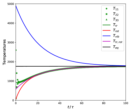
Figure 1: Relaxation of temperatures, on the right a zoom between $t=0$ and $t=25\tau$. ($\circ$) $T_{11}$, ($\square$) $T_{22}$ and ($\triangle$) $T_{33}$ are the components of the stress tensor. $T_{tr}$ (green), $T_{rot}$ (red) and $T_{vib}$ (blue) are respectively the temperatures of translation, rotation and vibration, while $T_{tr,rot}$ (purple) and $T_{eq}$ (black) are the translational-rotational temperature and temperature at equilibrium, respectively

In most cases $1<Z_{rot}<Z_{vib}$ and relaxation processes occur in a specific sequence (see [1] for empirical laws that are temperature dependent): first, the translational temperatures $T_{j,j}$ in the three directions $j=1,2,3$ relax towards the mean translational temperature $T_{tr}$, then the translational and rotational temperatures $T_{tr}$ and $T_{rot}$ relax towards the intermediate temperature $T_{tr,rot}$, and for longer times this temperature and the vibrational temperature $T_{vib}$ relax towards the equilibrium temperature $T_{eq}$ (see figure 1 in section 8 for an illustration).

4 An ES-BGK model with vibrations

In this section, our new ES-BGK model that accounts for vibrations of molecules is presented, and its main properties are stated and discussed.

4.1 Construction of the model

The evolution of the mass density of a gas in non-equilibrium is described by the Boltzmann equation

$$\partial_{t}f+v\cdot\nabla f=Q(f),$$ (18)

where $Q(f)$ is the Boltzmann collision operator.

A simpler relaxation BGK like model can be derived, as proposed in [14], where $Q(f)$ is replaced by $\frac{1}{\tau}(\mathcal{M}[f]-f)$, where $\tau$ is a relaxation time and $\mathcal{M}[f]$ is the generalized Maxwellian in velocity and energy, as defined by

$$\mathcal{M}[f](v,\varepsilon,i)=\mathcal{M}_{tr}[f](v)\mathcal{M}_{rot}[f](\varepsilon)\mathcal{M}_{vib}[f](i),$$ (19)

where

$$\mathcal{M}_{tr}[f](v)=\frac{\rho}{(2\pi RT_{eq})^{3/2}}\exp\left(-\frac{|v-u|^{2}}{2RT_{eq}}\right),$$

$$\mathcal{M}_{rot}[f](\varepsilon)=\frac{\Lambda(\delta)\varepsilon^{\frac{\delta-2}{2}}}{(RT_{eq})^{\delta/2}}\exp\left(-\frac{\varepsilon}{RT_{eq}}\right),$$

$${M}_{vib}[f](i)=\left(1-\exp(-T_{0}/T_{eq})\right)\exp\left(-i\frac{T_{0}}{T_{eq}}\right),$$

where exponential laws associated to vibrations and rotations are normalized by functions $(1-\exp(-T_{0}/T_{vib}^{rel}))$ and $\Lambda(\delta)=1/{\bf\Gamma}(\frac{\delta}{2})$, where ${\bf\Gamma}$ is the usual gamma function.

However, this model is too simple, since the single relaxation time cannot account for the various time scales of the original problem. Indeed, such a model gives the same value for rotational and vibrational relaxation times, and the same value for relaxation times of viscous and thermal fluxes, which gives the usual incorrect value $\Pr=1$ of the Prandtl number.

This problem can be fixed by using additional parameters in the model (at least 3 in this case). The correct Prandtl number for a monoatomic gas can be obtained by the ES-BGK approach [4], which has been extended later in [7] to account for a correct rotational time scale for polyatomic gases. Here, we extend this model to account for a correct vibrational time scale. Note that in this case, since the relation between temperature and energy is non linear, we find it more relevant to make an intensive use of the energy variable, that makes the derivation a bit different from that of [7].

Our ES-BGK collision operator is the following:

$$Q(f)=\frac{1}{\tau}(\mathcal{G}[f]-f),$$ (20)

where the Gaussian distribution $\mathcal{G}[f]$ is defined by

$$\mathcal{G}[f](v,\varepsilon,i)=\mathcal{G}_{tr}[f](v)\mathcal{G}_{rot}[f](\varepsilon)\mathcal{G}_{vib}[f](i),$$ (21)

with

$$\mathcal{G}_{tr}[f](v)=\frac{\rho}{\sqrt{\hbox{det}(2\pi\Pi)}}\exp\left(-\frac{1}{2}(v-u)^{T}\,\Pi^{-1}\,(v-u))\right),$$ (22)

$$\mathcal{G}_{rot}[f](\varepsilon)=\frac{\Lambda(\delta)}{(R{T_{rot}^{rel}})^{\delta/2}}\varepsilon^{\frac{\delta-2}{2}}\exp\left(-\frac{\varepsilon}{RT_{rot}^{rel}}\right),$$

$$\mathcal{G}_{vib}[f](i)=(1-\exp(-T_{0}/T_{vib}^{rel}))\exp\left(-i\frac{T_{0}}{T_{vib}^{rel}}\right).$$

Note that $\mathcal{G}_{tr}[f]$, $\mathcal{G}_{rot}[f]$ and $\mathcal{G}_{vib}[f]$ are distributions associated to the energies of translation, rotation and vibration of the molecules.

The covariance matrix $\Pi$ and the temperatures $T_{rot}^{rel}$ and $T_{vib}^{rel}$ are modifications of the stress tensor $\Theta$ and rotational and vibrational temperatures so as to fit different relaxation times to some given values, as it is explained below.

First, the corrected stress tensor $\Pi$ is defined by (with $I$ the identity matrix):

$$\Pi=\Gamma RT_{eq}I+(1-\Gamma)\left[\theta RT_{tr,rot}I+(1-\theta)(\nu\Theta+(1-\nu)RT_{tr}I)\right],$$ (23)

so that the hierarchy of relaxation processes explained in section 3.4 holds: (1) the directional temperatures $T_{j,j}$ (the diagonal elements of $\Theta$) first relax to $T_{tr}$ (this is governed by parameter $\nu$); (2) the translational temperature $T_{tr}$ relaxes to the intermediate temperature $T_{tr,rot}$ (this is governed by parameter $\theta$); (3) this temperature relaxes to the final equilibrium temperature $T_{eq}$, as governed by parameter $\Gamma$.

Now the relaxation temperatures $T_{rot}^{rel}$ and $T_{vib}^{rel}$, used in distributions $\mathcal{G}_{rot}$ and $\mathcal{G}_{vib}$, are defined with the same idea as the covariance matrix $\Pi$, except that we first write the relaxations in term of energies. Indeed, we define the relaxation energies for rotation and vibration by

$$\begin{split}&e_{rot}^{rel}=\Gamma e_{rot}(T_{eq})+(1-\Gamma)\left[\theta e_{rot}(T_{tr,rot})+(1-\theta)E_{rot}(f)\right],\\ &e_{vib}^{rel}=\Gamma e_{vib}(T_{eq})+(1-\Gamma)E_{vib}(f),\end{split}$$ (24)

and the corresponding relaxation temperatures are

$$T_{rot}^{rel}=e_{rot}^{-1}(e_{rot}^{rel}),\quad\text{ and }\quad T_{vib}^{rel}=e_{vib}^{-1}(e_{vib}^{rel}).$$ (25)

These definitions account for the relaxation of $T_{rot}$ to $T_{tr,rot}$ then to $T_{eq}$, and for the relaxation of $T_{vib}$ to $T_{eq}$ with rates that are consistent with the definition of $\Pi$.

Note that the relaxation rotational temperature $T_{rot}^{rel}$ can be equivalently defined by $T_{rot}^{rel}=\Gamma T_{eq}+(1-\Gamma)\left[\theta T_{tr,rot}+(1-\theta)T_{rot}\right]$, which is a simple extension of the definition given in [7]. However, the relaxation vibrational temperature $T_{vib}^{rel}$ cannot be defined in the same way: indeed, the nonlinearity of the function $e_{vib}$ would make the simpler definition $T_{vib}^{rel}=\Gamma T_{eq}+(1-\Gamma)T_{vib}$ not consistent with the energy conservation (see section 4.2).

This derivation shows that parameter $\theta$ is associated with transfers between translational and rotational energies and $\Gamma$ with transfers between translational-rotational and vibrational energies. It will be shown in section 5.1 that these parameters are related to $Z_{rot}$ and $Z_{vib}$ by the relations

$$\Gamma=\frac{1}{Z_{vib}},\quad\text{ and }\quad\theta=\frac{1/Z_{rot}-1/Z_{vib}}{1-1/Z_{vib}}.$$ (26)

Moreover, parameter $\nu$ will be used to fit the correct Prandtl number. It will be shown in section 5.2 that $\nu$ has to be set so that the Prandtl number $Pr$ is

$$Pr=\frac{1}{1-(1-\Gamma)(1-\theta)\nu}.$$ (27)

Finally, the relaxation time $\tau$ of the model is

$$\tau=\frac{\mu}{p}(1-(1-\Gamma)(1-\theta)\nu),$$

as it is proved in section 6.3.

4.2 Conservation properties

For the analysis of the conservation properties of our model, it is useful to define the relaxation energy of translation

$$e_{tr}^{rel}=\frac{1}{2}\operatorname{Tr}(\Pi)=\Gamma\frac{3}{2}RT_{eq}+(1-\Gamma)(\theta\frac{3}{2}RT_{tr,rot}+(1-\theta)\frac{3}{2}RT_{tr}),$$

and the corresponding relaxation temperature of translation which is

$$T_{tr}^{rel}=e_{tr}^{-1}(e_{tr}^{rel}),$$ (28)

that will be used later.

Then, note that this relation and the definition (24) of relaxation energies of rotation and vibration can be rewritten under the compact form

$$\begin{pmatrix}e_{tr}^{rel}\\ e_{rot}^{rel}\\ e_{vib}^{rel}\end{pmatrix}=\Gamma\begin{pmatrix}e_{tr}(T_{eq})\\ e_{rot}(T_{eq})\\ e_{vib}(T_{eq})\end{pmatrix}+(1-\Gamma)\begin{pmatrix}1-\frac{\delta\theta}{3+\delta}&\frac{3\theta}{3+\delta}&0\\ \frac{\delta\theta}{3+\delta}&1-\frac{3\theta}{3+\delta}&0\\ 0&0&1\end{pmatrix}\begin{pmatrix}E_{tr}(f)\\ E_{rot}(f)\\ E_{vib}(f)\end{pmatrix}.$$ (29)

Now, we state what are the first moments of ${\cal G}[f]$ that can be computed by standard integrals and series (see appendix D).

Proposition 4.1.

The Gaussian ${\cal G}[f]$ satisfies

$$\left\langle{\cal G}[f]\right\rangle_{v,\varepsilon,i}=\rho,$$ (30)

$$\left\langle v{\cal G}[f]\right\rangle_{v,\varepsilon,i}=\rho u,$$ (31)

$$\left\langle\frac{1}{2}|v-u|^{2}{\cal G}[f]\right\rangle_{v,\varepsilon,i}=\rho e_{tr}^{rel},\quad\left\langle\varepsilon{\cal G}[f]\right\rangle_{v,\varepsilon,i}=\rho e_{rot}^{rel},\quad\left\langle iRT_{0}{\cal G}[f]\right\rangle_{v,\varepsilon,i}=\rho e_{vib}^{rel}.$$ (32)

Then these properties can be used to prove the conservations properties of our kinetic model.

Proposition 4.2.

The collision operator of the ES-BGK model satisfies the conservation of mass, momentum, and energy:

$$\left\langle(1,v,\frac{1}{2}|v-u|^{2}+\varepsilon+iRT_{0})\frac{1}{\tau}({\cal G}[f]-f)\right\rangle_{v,\varepsilon,i}=0.$$

Proof.

The conservation of mass and momentum are obvious consequences of relations (30) and (31). For the conservation of energy, note that (32) and (29) imply

$$\begin{split}\left\langle(\frac{1}{2}|v-u|^{2}+\varepsilon+iRT_{0}){\cal G}[f]\right\rangle_{v,\varepsilon,i}&=\rho(e_{tr}^{rel}+e_{rot}^{rel}+e_{vib}^{rel})\\ &=\rho\Gamma(e_{tr}(T_{eq})+e_{rot}(T_{eq})+e_{vib}(T_{eq}))+\rho(1-\Gamma)(E_{tr}(f)+E_{rot}(f)+E_{int}(f))\\ &=\rho\Gamma E(f)+\rho(1-\Gamma)E(f)\\ &=\rho E(f)=\left\langle(\frac{1}{2}|v-u|^{2}+\varepsilon+iRT_{0})f\right\rangle_{v,\varepsilon,i},\end{split}$$

where we have used relations (13)–(15) and (8). ∎

4.3 Entropy

Andries et al. [7] proved that the ES-BGK model for polyatomic gases satisfies the entropy dissipation property. Since our ES-BGK model is an extension to include the energy of vibration of polyatomic gases we follow the same proof. First, the rotational energy variable $\varepsilon$ is transformed to the variable $I$ so that $\varepsilon=I^{2/\delta}$. With this new variable, the distribution function of the gas now is $g(t,x,v,I,i)$, defined such that $g(t,x,v,I,i)dI=f(t,x,v,\varepsilon,i)d\varepsilon$, which gives

$$g(t,x,v,I,i)=\frac{2}{\delta}\varepsilon^{1-\delta/2}f(t,x,v,\varepsilon,i).$$

Our ES-BGK model given by (18) and (20) now reads

$$\partial_{t}g+v\cdot\nabla g=\frac{1}{\tau}(\mathcal{G}[g]-g),$$ (33)

where the Gaussian distribution now reads:

$$\begin{split}\mathcal{G}[g]&=\rho\frac{2}{\delta}\frac{\Lambda(\delta)(1-\exp(-T_{0}/T_{vib}^{rel}))}{\sqrt{\det(2\pi\Pi)}(RT_{rot}^{rel})^{\delta/2}}\exp\left(-\frac{1}{2}(v-u)^{T}\,\Pi^{-1}\,(v-u)-\frac{I^{2/\delta}}{RT_{rot}^{rel}}-i\frac{T_{0}}{T_{vib}^{rel}}\right)\\ &=\exp(\boldsymbol{\alpha}^{T}\mathbf{m}),\end{split}$$ (34)

with

$$\Lambda(\delta)=\frac{\delta}{2}\left(\int_{\mathbb{R}}\exp(-I^{2/\delta})dI\right)^{-1},$$

$$\mathbf{m}=(1,v,v\otimes v,I^{2/\delta},iRT_{0})^{T},$$

$$\boldsymbol{\alpha}=\left(\log\left(\frac{2}{\delta}\frac{\rho\Lambda(\delta)(1-\exp(-T_{0}/T_{vib}^{rel}))}{\sqrt{\det(2\pi\Pi)}(RT_{rot}^{rel})^{\delta/2}}\right)-\frac{1}{2}u^{T}\Pi^{-1}u,\Pi^{-1}u,-\frac{1}{2}\Pi^{-1},-\frac{1}{RT_{rot}^{rel}},-\frac{1}{RT_{vib}^{rel}}\right).$$

The corresponding Maxwellian equilibrium now is

$${\cal M}[g]=\rho\frac{2}{\delta}\frac{\Lambda(\delta)(1-\exp(-T_{0}/T_{eq}))}{(2\Pi RT_{eq})^{3/2}(RT_{eq})^{\delta/2}}\exp\left(-\frac{|v-u|^{2}}{2RT_{eq}}-\frac{I^{2/\delta}}{RT_{eq}}-i\frac{T_{0}}{T_{eq}}\right).$$

This transformation makes all the proofs of this section much simpler. Now we give the conditions on which our model is well defined, and we state its entropy property.

Proposition 4.3.

For parameters $-1/2\leq\nu<1$, $0\leq\theta<1$, and $0\leq\Gamma<1$ we have:

1. For symmetric positive definite tensor $\Theta$ and positive temperatures $T_{tr,rot}$ and $T_{tr}$, the tensor $\Pi$ defined by (23) is symmetric positive definite.

2. (Entropy minimization) If $g$ is a non-negative distribution, then the Gaussian distribution $\mathcal{G}[g]$ defined by (34) is the unique minimizer of the entropy $\mathbb{H}(g)=\left\langle g\log g-g\right\rangle_{v,I,i}$ on the set ${\cal X}=\{\phi\geq 0,\ \left\langle\mathbf{m}\phi\right\rangle_{v,I,i}=\left(\rho,\rho u,\rho(u\otimes u+\Pi),\rho e_{rot}^{rel},\rho e_{vib}^{rel}\right)\}.$

3. (H-theorem) The ES-BGK model (33) satisfies

   $$\partial_{t}\mathbb{H}(g)+\nabla\cdot\left\langle v(g\log g-g)\right\rangle_{v,I,i}=\left\langle\frac{1}{\tau}(\mathcal{G}[g]-g)\log g\right\rangle_{v,I,i}\leq 0,$$

4. (Equilibrium) If $g=\mathcal{G}[g]$, then $g=\mathcal{M}[g]$.

Proof of Property 1..

We first rewrite $\Pi$ as follows: we define the intermediate stress tensor $A=\nu\Theta+(1-\nu)RT_{tr}I$ associated to the relaxation phenomenon for the translation mode, and the tensor $B=(1-\theta)A+\theta RT_{tr,rot}I$ associated to the relaxation of the rotational mode, such that (23) reads $\Pi=(1-\Gamma)B+\Gamma RT_{eq}I$. Andries et al. [7] have proved that tensor $A$ is positive definite for $\nu\in[-1/2,1]$. Now, for $\theta\in[0,1]$, since $B$ is a convex combination of $A$ and $RT_{tr,rot}I$, it is also symmetric and positive definite. Finally, for $\Gamma\in[0,1]$, $\Pi$ is a convex combination of $B$ and $RT_{eq}I$, and hence is symmetric and positive definite too. ∎

Proof of Property 2..

First, note that by construction, ${\cal G}[g]$ is in set ${\cal X}$. Then, since the functional $g\mapsto\mathbb{H}(g)$ is convex, then we have

$$\mathbb{H}(\mathcal{G}[g])\leq\mathbb{H}(\phi)-\mathbb{H}^{\prime}(\mathcal{G}[g])(\phi-\mathcal{G}[g])$$

for every $\phi$ in ${\cal X}$. Moreover, we have

$$\begin{split}\mathbb{H}^{\prime}(\mathcal{G}[g])(\phi-\mathcal{G}[g])&=\left\langle(\phi-\mathcal{G}[g])\log\mathcal{G}[g]\right\rangle_{v,I,i}\\ &=\left\langle(\phi-\mathcal{G}[g])\boldsymbol{\alpha}^{T}\mathbf{m}\right\rangle_{v,I,i}\\ &=0,\end{split}$$

since both $\mathcal{G}[g]$ and $\phi$ are in ${\cal X}$. Consequently $\mathbb{H}(\mathcal{G}[g])\leq\mathbb{H}(\phi)$ for every $\phi$ in ${\cal X}$, which concludes the proof.

∎

Proof of property 3..

This proof is decomposed into 4 steps.

Step 1: entropy inequality.

First, note that with elementary calculus, (33) implies

$$\partial_{t}\mathbb{H}(g)+\nabla\cdot\left\langle v(g\log g-g)\right\rangle_{v,I,i}=\frac{1}{\tau}\mathbb{H}^{\prime}(g)(\mathcal{G}[g]-g).$$

Then, since $\mathbb{H}$ is convex, the right-hand side of the previous equality satisfies

$$\mathbb{H}^{\prime}(g)(\mathcal{G}[g]-g)\leq\mathbb{H}(\mathcal{G}[g])-\mathbb{H}(g).$$

Consequently, the H-theorem is obtained if we can prove that

$$\mathbb{H}(\mathcal{G}[g])\leq\mathbb{H}(g).$$ (35)

Note that this is not obvious, since $g$ is not in ${\cal X}$.

Step 2: entropy minima on different sets.

It is convenient to define, for every macroscopic quantities $\rho$, $u$, $\Pi$, $T_{rot}^{rel}$ and $T_{vib}^{rel}$ the minimum of entropy $\mathbb{H}$ on $\cal X$, and we set

$$S(\rho,u,\Pi,T_{rot}^{rel},T_{vib}^{rel})=\min\left\{\mathbb{H}(\phi),\phi\geq 0\text{ s.t.}\left\langle\mathbf{m}\phi\right\rangle_{v,I,i}=\left(\rho,\rho u,\rho(u\otimes u+\Pi),\rho e_{rot}^{rel},\rho e_{vib}^{rel}\right)\right\}.$$

Property 2 implies

$$S(\rho,u,\Pi,T_{rot}^{rel},T_{vib}^{rel})=\mathbb{H}(\mathcal{G}[g]).$$

Now we define a second entropy minimization problem, based on the moments of $g$. Namely

$$S(\rho,u,\Theta,T_{rot},T_{vib})=\min\left\{\mathbb{H}(\phi),\phi\geq 0\text{ s.t.}\left\langle\mathbf{m}\phi\right\rangle_{v,I,i}=\left(\rho,\rho u,\rho(u\otimes u+\Theta),\rho E_{rot}(f),\rho E_{vib}(f)\right)\right\}.$$

Here, by definition $g$ belongs to the minimization set, and therefore

$$S(\rho,u,\Theta,T_{rot},T_{vib})\leq\mathbb{H}(g).$$

Therefore, a sufficient condition to have (35) is $S(\rho,u,\Pi,T_{rot}^{rel},T_{vib}^{rel})\leq S(\rho,u,\Theta,T_{rot},T_{vib})$, which is rewritten as

$$\Delta S=S(\rho,u,\Pi,T_{rot}^{rel},T_{vib}^{rel})-S(\rho,u,\Theta,T_{rot},T_{vib})\leq 0.$$ (36)

This entropy difference is now analyzed in the following.

Step 3: entropy difference

A direct calculation gives

$$S(\rho,u,\Pi,T_{rot}^{rel},T_{vib}^{rel})=\rho\log\left(\rho\frac{2}{\delta}\frac{\Lambda(\delta)(1-\exp(-T_{0}/T_{vib}^{rel}))}{\sqrt{\det(2\pi\Pi)}(RT_{rot}^{rel})^{\delta/2}}\right)-\rho\frac{5+\delta+\delta_{v}(T_{vib}^{rel})}{2}.$$

A similar relation is deduced for $S(\rho,u,\Theta,T_{rot},T_{vib})$ and we get

$$\Delta S =\frac{1}{2}\rho\log\left(\frac{\det\Theta}{\det\Pi}\left(\frac{T_{rot}}{T_{rot}^{rel}}\right)^{\delta}\left(\frac{(1-\exp(-T_{0}/T_{vib}^{rel}))}{(1-\exp(-T_{0}/T_{vib}))}\right)^{2}\right)-\rho\frac{\delta_{v}(T_{vib}^{rel})-\delta_{v}(T_{vib})}{2},$$

$$=\frac{1}{2}\rho\log\left(\frac{\det\Theta}{\det\Pi}\left(\frac{E_{rot}(f)}{e_{rot}^{rel}}\right)^{\delta}\left(\frac{RT_{0}+E_{vib}(f)}{RT_{0}+e_{vib}^{rel}}\right)^{2}\right)-\rho\frac{\delta_{v}(T_{vib}^{rel})-\delta_{v}(T_{vib})}{2}$$

where we have used relations (2), (12), and (25) to obtain the last equality.

First, the following result is admitted (see the proof in appendix A):

$$\frac{\det\Theta}{\det\Pi}\leq\left(\frac{E_{tr}(f)}{e_{tr}^{rel}}\right)^{3}.$$ (37)

This allows us to write the following inequality, as function of energies only:

$$\Delta S\leq\frac{1}{2}\rho\log\left(\left(\frac{E_{tr}(f)}{e_{tr}^{rel}}\right)^{3}\left(\frac{E_{rot}(f)}{e_{rot}^{rel}}\right)^{\delta}\left(\frac{RT_{0}+E_{vib}(f)}{RT_{0}+e_{vib}^{rel}}\right)^{2}\right)-\rho\frac{\delta_{v}(T_{vib}^{rel})-\delta_{v}(T_{vib})}{2}.$$

After expansion, this inequality reads as

$$\Delta S\leq\frac{\rho}{R}\left(\mathcal{S}(E_{tr}(f),E_{rot}(f),E_{vib}(f))-\mathcal{S}(e^{rel}_{tr},e^{rel}_{rot},e^{rel}_{vib})\right),$$ (38)

where we have introduced the new energy functional $\mathcal{S}$, defined for every energy triplet $(e_{1},e_{2},e_{3})$ by

$$\mathcal{S}(e_{1},e_{2},e_{3})=R\left(\frac{3}{2}\log(e_{1})+\frac{\delta}{2}\log(e_{2})+\log\left(1+\frac{e_{3}}{RT_{0}}\right)+\frac{e_{3}}{RT_{0}}\log\left(1+\frac{RT_{0}}{e_{3}}\right)\right).$$

Note that to obtain (38), we also have replaced $\delta_{v}$ by its definition (17) and the temperatures of vibration have been replaced by their corresponding energies.

Now it is clear that a sufficient condition to have $\Delta S\leq 0$ is

$$\mathcal{S}(E_{tr}(f),E_{rot}(f),E_{vib}(f))\leq\mathcal{S}(e^{rel}_{tr},e^{rel}_{rot},e^{rel}_{vib}),$$ (39)

which is proved in the last step.

Step 4: proof of (39)

The usual argument to conclude an entropy inequality is a convexity property. Here, our functional $\mathcal{S}$ can easily be seen to be concave (see appendix B). However, since the right-hand side of (39) is not at equilibrium, a direct use of the convexity inequality does not work here. Instead, we find it simpler, and physically relevant, to use successively two paths, based on parameters $\theta$ and $\Gamma$. Indeed, note that relaxation energies $(e^{rel}_{tr},e^{rel}_{rot},e^{rel}_{vib})$ depend on $\theta$ and $\Gamma$ (see (29)). Then we set

$$s(\theta,\Gamma)=\mathcal{S}(e^{rel}_{tr},e^{rel}_{rot},e^{rel}_{vib}).$$

From (29), it is clear that $s(0,0)=\mathcal{S}(E_{tr}(f),E_{rot}(f),E_{vib}(f))$ since the relaxation energies reduce to the internal energies of $f$ for such values of $\theta$ and $\Gamma$. Consequently, inequality (39) reduces to

$$s(0,0)\leq s(\theta,\Gamma).$$ (40)

The idea is now to decompose inequality (40) into two embedded inequalities

$$s(0,0)\leq s(\theta,0)\leq s(\theta,\Gamma).$$ (41)

We start with the second inequality and consider the variation of $s$ with respect to $\Gamma$. Elementary calculus shows that

$$\begin{split}\frac{\partial s}{\partial\Gamma}(\theta,\Gamma)&=\frac{1}{T_{tr}^{rel}}\left(e_{tr}(T_{eq})-\left(1-\frac{\delta\theta}{3+\delta}\right)E_{tr}(f)-\frac{3\theta}{3+\delta}E_{rot}(f)\right)\\ &+\frac{1}{T_{rot}^{rel}}\left(e_{rot}(T_{eq})-\left(1-\frac{3\theta}{3+\delta}\right)E_{rot}(f)-\frac{\delta\theta}{3+\delta}E_{tr}(f)\right)\\ &+\frac{1}{T_{vib}^{rel}}\left(e_{vib}(T_{eq})-E_{vib}(f)\right),\end{split}$$ (42)

and

$$\begin{split}\frac{\partial^{2}s}{\partial\Gamma^{2}}(\theta,\Gamma)&=\partial_{1,1}\mathcal{S}(e_{tr}^{rel},e_{rot}^{rel},e_{vib}^{rel})\left(e_{tr}(T_{eq})-\left(1-\frac{\delta\theta}{3+\delta}\right)E_{tr}(f)-\frac{3\theta}{3+\delta}E_{rot}(f)\right)^{2}\\ &+\partial_{2,2}\mathcal{S}(e_{tr}^{rel},e_{rot}^{rel},e_{vib}^{rel})\left(e_{rot}(T_{eq})-\left(1-\frac{3\theta}{3+\delta}\right)E_{rot}(f)-\frac{\delta\theta}{3+\delta}E_{tr}(f)\right)^{2}\\ &+\partial_{3,3}\mathcal{S}(e_{tr}^{rel},e_{rot}^{rel},e_{vib}^{rel})\left(e_{vib}(T_{eq})-E_{vib}(f)\right)^{2},\end{split}$$

and the reader is referred to appendix B for the computation of the partial derivatives of $\mathcal{S}$. The previous relation shows that $s$ is a concave function of $\Gamma$. Moreover, note that for $\Gamma=1$, relation (29) shows that all the relaxation energies are equal to the equilibrium energy, and hence all the relaxation temperatures are equal to $T_{eq}$. When this is used into (42), we find that $\frac{\partial s}{\partial\Gamma}(\theta,1)=0$. With the concavity property, this proves that $s$ is an increasing function of $\Gamma$ on the interval $[0,1]$, and this proves the second inequality of (41).

For the first inequality of (41), we set $\Gamma$ to 0, and we study the variation of $s(\theta,0)$ with respect to $\theta$. Again, elementary calculus shows that $\frac{\partial^{2}s}{\partial\theta^{2}}(\theta,0)\leq 0$, and hence $s(\theta,0)$ is a concave function of $\theta$. Moreover, we find

$$\begin{split}\frac{\partial s}{\partial\theta}(0,0)=-\frac{3\delta}{2(3+\delta)}R(T_{tr}-T_{rot})(\frac{1}{T_{tr}}-\frac{1}{T_{rot}}),\end{split}$$ (43)

which implies that $s(\theta,0)$ is a non decreasing function of $\theta$. Consequently, this gives the first inequality of (41) which concludes the proof of (39), and hence of (35), and the proof of the H-theorem is now complete.

∎

Proof of property 4..

At equilibrium $g=\mathcal{G}[g]$ and hence $\Theta=\Pi$, $E_{rot}(g)=e_{rot}^{rel}$, and $E_{vib}(g)=e_{vib}^{rel}$. Then it is easy to see that relations (23)–(25) imply $T_{tr}=T_{rot}=T_{vib}=T_{tr,rot}=T_{rot}^{rel}=T_{vib}^{rel}=T_{eq}$ and then $\Theta=RT_{eq}I$. Consequently, $\mathcal{G}[g]=\mathcal{M}[g]$ and then $g=\mathcal{M}[g]$. ∎

Remark 4.1.

Of course, the equivalent H-theorem for our initial model (with function $f$ and variable $\varepsilon$) can then be obtained by using the change of variable $\varepsilon=I^{\frac{2}{\delta}}$. However, note that the entropy functional now reads $\mathbb{H}(f)=\langle f\log(f/\varepsilon^{\frac{\delta}{2}-1})\rangle_{v,\varepsilon,i}$.

5 Relaxation phenomena

In this section, we resolve the local relaxation equations for energies, stress tensor, and heat flux. This give us the relations between parameters $\Gamma$, $\theta$, and $\nu$ of our model and the vibrational and rotation collision numbers $Z_{vib}$, $Z_{rot}$, and the Prandtl number.

5.1 Relaxation rates of translational, rotational and vibrational energies

The energy of translation, rotation and vibration are transferred from one mode to another one during inter-molecular collisions. These transfers are described by local relaxations obtained as moments of our ES-BGK model (in a space homogeneous case). Indeed, our model (18)–(20) is multiplied by $\frac{1}{2}|v-u|^{2}$, $\varepsilon$, $iRT_{0}$, and integrated w.r.t $v$, $\varepsilon$, and $i$, and we use closure relations (29) to find

$$\frac{d}{dt}\begin{pmatrix}E_{tr}(f)\\ E_{rot}(f)\\ E_{vib}(f)\end{pmatrix}=\frac{\Gamma}{\tau}\begin{pmatrix}e_{tr}(T_{eq})-E_{tr}(f)\\ e_{rot}(T_{eq})-E_{rot}(f)\\ e_{vib}(T_{eq})-E_{vib}(f)\end{pmatrix}+\frac{1-\Gamma}{\tau}\begin{pmatrix}-\frac{\delta\theta}{3+\delta}&\frac{3\theta}{3+\delta}&0\\ \frac{\delta\theta}{3+\delta}&-\frac{3\theta}{3+\delta}&0\\ 0&0&0\end{pmatrix}\begin{pmatrix}E_{tr}(f)\\ E_{rot}(f)\\ E_{vib}(f)\end{pmatrix}$$ (44)

The last equation has to be consistent with the Landau-Teller relaxation equation that describes the relaxation of the macroscopic energy of vibration to equilibrium, at a relaxation rate $\tau_{vib}=\tau Z_{vib}$. The second equation has to be consistent with the Jeans relaxation equation, which plays the same role for rotational energy, at the rate $\tau_{rot}=\tau Z_{rot}$. Moreover, this equation should also be consistent with the fast relaxation of $T_{tr}$ and $T_{rot}$ towards $T_{tr,rot}$ (see section 3.4).

Now we assume parameters $\tau$, $\Gamma$, and $\theta$ to be constant, and we solve these equations to find

$$E_{vib}(f(t)) =e_{vib}(T_{eq})+(E_{vib}(f(0))-e_{vib}(T_{eq}))\exp\left(-\frac{\Gamma}{\tau}t\right),$$

$$E_{rot}(f(t)) =e_{rot}(T_{eq})$$

$$\quad+\left[E_{rot}(f(0))-e_{rot}(T_{eq})+\frac{\delta}{3+\delta}(E_{vib}(f(0))-e_{vib}(T_{eq}))\right]\exp\left(-\frac{1-(1-\Gamma)(1-\theta)}{\tau}t\right)$$

$$\quad-\frac{\delta}{3+\delta}(E_{vib}(f(0))-e_{vib}(T_{eq}))\exp\left(-\frac{\Gamma}{\tau}t\right).$$

From these equations we deduce that:

$$Z_{vib}=\frac{1}{\Gamma},\quad Z_{rot}=\frac{1}{1-(1-\Gamma)(1-\theta)},$$

or equivalently $\Gamma=1/Z_{vib}$ and $\theta={(Z_{vib}-Z_{rot})}/{((Z_{vib}-1)Z_{rot})}$.

Since we want the rotational and vibrational collision numbers such that $1<Z_{rot}<Z_{vib}$ (see section 3.4), then the previous definition gives the restriction $0\leq\theta<1$ and $0\leq\Gamma<1$. Case $\theta=0$ gives $Z_{rot}=Z_{vib}$ which means that vibration modes relax as fast as rotation modes. In case $\Gamma=0$, then $Z_{vib}=+\infty$ and $Z_{rot}=1/\theta$, and we find the polyatomic ES-BGK model without vibrations of Andries et al. [7].

The equivalent relaxations of temperatures are

$$R(T_{tr,rot}-T_{eq})= -\frac{2}{3+\delta}(E_{vib}(f(0))-e_{vib}(T_{eq}))\exp\left(-\frac{t}{\tau Z_{vib}}\right)$$ (45)

$$R(T_{tr}-T_{tr,rot})= -\frac{2}{3}\left[E_{rot}(f(0))-e_{rot}(T_{eq})+\frac{\delta}{3+\delta}(E_{vib}(f(0))-e_{vib}(T_{eq}))\right]\exp\left(-\frac{t}{\tau Z_{rot}}\right)$$

These two expressions will be used in the numerical tests of section 8 to check the correct rates of convergence to equilibrium.

5.2 Relaxation of stress and heat flux

Relaxation equations for stress tensor and heat flux are obtained by multiplying the kinetic equation (18) by $(v-u)\otimes(v-u)$ and $(\frac{1}{2}|v-u|^{2}+\varepsilon+iRT_{0})(v-u)$ and integrating w.r.t $v$,$\varepsilon$ and $i$ to get, in the space homogeneous case :

$$\frac{d}{dt}\Theta=\frac{1}{\tau}((1-\Gamma)(1-\theta)(1-\nu)(RT_{tr}I-\Theta)+(1-\Gamma)\theta(RT_{tr,rot}I-\Theta)+\Gamma(RT_{eq}I-\Theta)),$$ (46)

$$\frac{d}{dt}q=-\frac{1}{\tau}q.$$ (47)

Since $\operatorname{Tr}(\Theta)=3RT_{tr}$, taking the trace of (46) gives

$$\frac{d}{dt}RT_{tr}=\frac{1}{\tau}\left((1-\Gamma)\theta(RT_{tr,rot}-RT_{tr})+\Gamma(RT_{eq}-RT_{tr})\right).$$

This equation is subtracted to (46) to get

$$\frac{d}{dt}(\Theta-RT_{tr}I)=-\frac{1}{\tau}(1-(1-\theta)(1-\Gamma)\nu)(\Theta-RT_{tr}I).$$

This shows that for large times, the stress tensor tends to $RT_{tr}I$, while the heat flux tends to 0. More precisely, for $\nu$, $\theta$, $\Gamma$ and $\tau$ constant, we have the analytic solutions:

$$\Theta(t)-RT_{tr}(t)I=(\Theta(0)-RT_{tr}(0)I)\exp\left(-(1-(1-\Gamma)(1-\theta)\nu)\frac{t}{\tau}\right),$$

$$q(t)=q(0)\exp\left(-\frac{t}{\tau}\right).$$

The Prandtl number can be viewed as the ratio between the relaxation times of these two processes, and we get:

$$\Pr=\frac{1}{1-(1-\Gamma)(1-\theta)\nu}.$$

Incidentally, this value will be checked numerically in section 8 by computing the ratio

$$\frac{\log(|q_{i}(t)/q_{i}(0)|)}{\log(|(\Theta_{ii}(t)-RT_{tr}(t))/(\Theta_{ii}(0)-RT_{tr}(0))|)}$$ (48)

for $i=1,2,3$.

6 Chapman-Enskog analysis

The conservation laws are obtained by multiplying (18) by the vector $1$, $v$, and $\frac{1}{2}|v|^{2}$ and then by integrating it to get:

$$\partial_{t}\rho+\nabla\cdot(\rho u)=0,$$ (49)

$$\partial_{t}(\rho u)+\nabla\cdot(\rho u\otimes u)+\nabla\cdot\Sigma(f)=0,$$

$$\partial_{t}\mathcal{E}+\nabla\cdot(\mathcal{E}u)+\nabla\cdot\Sigma(f)+\nabla\cdot q(f)=0,$$

where $\mathcal{E}=\langle(\frac{1}{2}|v|^{2}+\varepsilon+iRT_{0})f\rangle_{v,\varepsilon,i}=\frac{1}{2}\rho|u|^{2}+\rho E(f)$ is the total energy density, $\Sigma(f)=\langle(v-u)\otimes(v-u)f\rangle_{v,\varepsilon,i}=\rho\Theta$ is the stress tensor and $q(f)=\langle(\frac{1}{2}|v-u|^{2}+\varepsilon+iRT_{0})(v-u)f\rangle_{v,\varepsilon,i}$ is the heat flux.

If we have some characteristic values of length, time, velocity, density, and temperature, our ES-BGK model (18)–(20) can be non-dimensionalized. This equation reads

$$\partial_{t}f+v\cdot\nabla f=\frac{1}{{\rm Kn}\,\tau}(\mathcal{G}[f]-f),$$ (50)

where ${\rm Kn}$ is the Knudsen number which is the ratio between the mean free path and a macroscopic length scale. For simplicity, here we use the same notations for the non-dimensional variables as for the dimensional ones.

The Chapman-Enskog analysis consists in approximating the stress tensor and the heat flux at first and second order with respect to the Knudsen number, which gives compressible Euler equations and compressible Navier-Stokes equations, respectively.

6.1 Euler asymptotics

At equilibrium $f$, is equal to the equilibrium Maxwellian distribution. Even in non-equilibrium, when ${\rm Kn}$ is very small the gas is very close to its equilibrium state, and equation (18)–(20) gives

$$f=\mathcal{M}[f]+O({\rm Kn}),$$ (51)

if in addition $f$ and its time and space derivatives are $O(1)$ w.r.t ${\rm Kn}$. Then definition (11) gives

$$\Sigma(f)=pI+O({\rm Kn}),\qquad q(f)=O({\rm Kn}),$$ (52)

where we denote by $p=\rho RT_{eq}$ the pressure at equilibrium.

These last relations are used into conservation laws (49) to get the compressible Euler equations with first order reminder:

$$\partial_{t}\rho+\nabla\cdot(\rho u)=0,$$ (53)

$$\partial_{t}(\rho u)+\nabla\cdot(\rho u\otimes u)+\nabla p=O({\rm Kn}),$$

$$\partial_{t}\mathcal{E}+\nabla\cdot\left((\mathcal{E}+p)u\right)=O({\rm Kn}).$$

The non-conservative form of these equations is

$$\partial_{t}\rho+u\cdot\nabla\rho+\rho\nabla\cdot u=0,$$ (54)

$$\partial_{t}u+(u\cdot\nabla)u+\frac{1}{\rho}\nabla p=O({\rm Kn}),$$

$$\partial_{t}T_{eq}+u\cdot\nabla T_{eq}+T_{eq}C\nabla\cdot u=O({\rm Kn}),$$

with $C=\frac{R}{c_{v}(T_{eq})}$, and $c_{v}(T_{eq})=\frac{\partial e(T_{eq})}{\partial T_{eq}}$ is the heat capacity at constant volume of the gas, which is temperature dependent here due to vibration modes (see equations (14) and (15)).

Moreover, simple calculations give $E_{\alpha}(\mathcal{M}[f])=e_{\alpha}(T_{eq})$ for $\alpha=tr,rot,vib$. Since the energy functions are regular, our expansion $f=\mathcal{M}[f]+O({\rm Kn})$ and relations (12) and (16) give

$$T_{tr}=T_{eq}+O({\rm Kn}),\ T_{rot}=T_{eq}+O({\rm Kn}),\ T_{vib}=T_{eq}+O({\rm Kn}),\ T_{tr,rot}=T_{eq}+O({\rm Kn}).$$ (55)

The Navier-Stokes equations are obtained by looking for a second order expansion of $f$. In the following section, we first derive useful second order expansions of energies and tensor $\Pi$ that are used in our model.

6.2 Energy and tensor relations at second order

First, (18) is multiplied by $\frac{1}{2}|v-u|^{2}$, $\varepsilon$, and $iRT_{0}$ and integrated w.r.t $v$, $\varepsilon$, and $i$. We use relations (52), (55), and (29) to get

$$\partial_{t}\begin{pmatrix}E_{tr}(f)\\ E_{rot}(f)\\ E_{vib}(f)\end{pmatrix}+u\cdot\nabla\begin{pmatrix}E_{tr}(f)\\ E_{rot}(f)\\ E_{vib}(f)\end{pmatrix}+\begin{pmatrix}RT_{eq}\nabla\cdot u\\ 0\\ 0\end{pmatrix}+O({\rm Kn})=\frac{\Gamma}{{\rm Kn}\tau}\begin{pmatrix}e_{tr}(T_{eq})\\ e_{rot}(T_{eq})\\ e_{vib}(T_{eq})\end{pmatrix}+\frac{1}{{\rm Kn}\tau}D\begin{pmatrix}E_{tr}(f)\\ E_{rot}(f)\\ E_{vib}(f)\end{pmatrix}$$ (56)

with

$$D=\begin{pmatrix}-\frac{(1-\Gamma)\delta\theta}{3+\delta}-\Gamma&\frac{3(1-\Gamma)\theta}{3+\delta}&0\\ \frac{\delta(1-\Gamma)\theta}{3+\delta}&-\frac{3(1-\Gamma)\theta}{3+\delta}-\Gamma&0\\ 0&0&-\Gamma\end{pmatrix}.$$

Note that the eigenvalues of $D$ are $-\Gamma$, $-\Gamma$, and $-\Gamma-(1-\Gamma)\theta$ so that (56) is indeed a relaxation process, and also that $D$ is invertible.

Moreover, from (12), we deduce the differential relation $dE_{\alpha}(f)=e^{\prime}_{\alpha}(T_{\alpha})dT_{\alpha}$, for $\alpha=tr,rot,vib$. Then, using (55) and the last equation of (54), we get

$$\partial_{t}\begin{pmatrix}E_{tr}(f)\\ E_{rot}(f)\\ E_{vib}(f)\end{pmatrix}+u\cdot\nabla\begin{pmatrix}E_{tr}(f)\\ E_{rot}(f)\\ E_{vib}(f)\end{pmatrix}=-\begin{pmatrix}e_{tr}^{\prime}(T_{eq})CT_{eq}\\ e_{rot}^{\prime}(T_{eq})CT_{eq}\\ e_{vib}^{\prime}(T_{eq})CT_{eq}\end{pmatrix}\nabla\cdot u+O({\rm Kn}).$$ (57)

Finally, relations (56) and (57) give the following system

$$\Gamma\begin{pmatrix}e_{tr}(T_{eq})\\ e_{rot}(T_{eq})\\ e_{vib}(T_{eq})\end{pmatrix}+D\begin{pmatrix}E_{tr}(f)\\ E_{rot}(f)\\ E_{vib}(f)\end{pmatrix}=-{\rm Kn}\tau\begin{pmatrix}e_{tr}^{\prime}(T_{eq})CT_{eq}-RT_{eq}\\ e_{rot}^{\prime}(T_{eq})CT_{eq}\\ e_{vib}^{\prime}(T_{eq})CT_{eq}\end{pmatrix}\nabla\cdot u+O({\rm Kn}^{2})$$

that has to be solved to get second order expansion of energies as functions of the equilibrium temperature and of the divergence of $u$. We only write here the relations that will be useful to derive the Navier-Stokes hydrodynamics:

$$E_{tr}(f)=e_{tr}(T_{eq})+\frac{{\rm Kn}\tau}{\Gamma}\left(\frac{3}{2}C-\frac{1}{\Gamma+(1-\Gamma)\theta}\left(\Gamma+\frac{3(1-\Gamma)\theta}{3+\delta}\right)\right)RT_{eq}\nabla\cdot u+O({\rm Kn}^{2}),$$

$$E_{tr,rot}(f)=e_{tr,rot}(T_{eq})+\frac{{\rm Kn}\tau}{\Gamma}\left(\frac{3+\delta}{2}C-1\right)RT_{eq}\nabla\cdot u+O({\rm Kn}^{2}).$$

Similar relations are readily derived for temperatures $T_{tr}$ and $T_{tr,rot}$ by using (12) and (16), and therefore, (23) can now be used to derive the second order expansion of tensor $\Pi$:

$$\begin{split}\Pi=&(1-(1-\Gamma)(1-\theta)\nu)RT_{eq}I+(1-\Gamma)(1-\theta)\nu\Theta\\ &+(1-\Gamma)\theta\frac{{\rm Kn}\tau}{\Gamma}\left(C-\frac{2}{3+\delta}\right)RT_{eq}\nabla\cdot u\\ &+(1-\Gamma)(1-\theta)(1-\nu)\frac{{\rm Kn}\tau}{\Gamma}\left(C-\frac{1}{\Gamma+(1-\Gamma)\theta)}\frac{2}{3}\left(\Gamma+\frac{3(1-\Gamma)\theta}{3+\delta}\right)\right)RT_{eq}\nabla\cdot u\\ &+O({\rm Kn}^{2}).\end{split}$$ (58)

Finally, we find it convenient to define the following three quantities

$$\gamma_{mono}=\frac{5}{3},\quad\gamma_{rot}=\frac{5+\delta}{3+\delta},\quad\gamma=1+\frac{R}{c_{v}(T_{eq})}\\$$ (59)

that are nothing but heat capacity ratios for a monoatomic gas, a polyatomic gas with rotational modes only, and the present gas with rotational and vibrational modes, respectively. Then $\Pi$ can be rewritten as

$$\begin{split}\Pi=&(1-(1-\Gamma)(1-\theta)\nu)RT_{eq}I+(1-\Gamma)(1-\theta)\nu\Theta\\ &-\left(\frac{(1-\Gamma)(1-\theta)(1-\nu)}{1-(1-\Gamma)(1-\theta)}(\gamma_{mono}-\gamma_{rot})+\frac{(1-\Gamma)(1-(1-\theta)\nu)}{\Gamma}(\gamma_{rot}-\gamma)\right){\rm Kn}\tau RT_{eq}\nabla\cdot u\\ &+O({\rm Kn}^{2}).\end{split}$$ (60)

6.3 Navier-Stokes limit

We first state our main result.

Proposition 6.1.

The moments of $f$, solution of the ES-BGK model (18), satisfy the compressible Navier-Stokes equations up to $O({\rm Kn}^{2})$:

$$\partial_{t}\rho+\nabla\cdot(\rho u)=O({\rm Kn}^{2}),$$

$$\partial_{t}(\rho u)+\nabla\cdot(\rho u\otimes u)+\nabla p=-\nabla\cdot\sigma+O({\rm Kn}^{2}),$$

$$\partial_{t}\mathcal{E}+\nabla\cdot(\mathcal{E}+p)u=-\nabla\cdot q-\nabla\cdot(\sigma u)+O({\rm Kn}^{2}),$$

where, in dimensional form, the shear stress tensor and the heat flux are given by

$$\sigma=-\mu\left(\nabla u+(\nabla u)^{T}-\alpha\nabla\cdot uI\right),\quad q=-\kappa\nabla T,$$

the viscosity and heat transfer coefficient are

$$\mu=\frac{\tau p}{1-(1-\Gamma)(1-\theta)\nu},\qquad\kappa=(1-(1-\Gamma)(1-\theta)\nu)\mu c_{p},$$

the second viscosity coefficient is

$$\alpha=(\gamma-1)-\frac{(1-\Gamma)(1-\theta)(1-\nu)}{1-(1-\Gamma)(1-\theta)}(\gamma_{mono}-\gamma_{rot})-\frac{(1-\Gamma)(1-(1-\theta)\nu)}{\Gamma}(\gamma_{rot}-\gamma),$$

and the Prandtl number is

$$Pr=\frac{\mu c_{p}}{\kappa}=\frac{1}{1-(1-\Gamma)(1-\theta)\nu},$$

while $c_{p}=\frac{\partial h}{\partial T_{eq}}$ is the heat capacity at constant pressure, where $h=e(T_{eq})+p/\rho$ is the enthalpy. The heat capacity ratios $\gamma$, $\gamma_{mono}$, $\gamma_{rot}$ are defined in (59).

Proof.

First, (50) yields

$$f=\mathcal{G}[f]-\tau{\rm Kn}(\partial_{t}\mathcal{M}[f]+v\cdot\nabla\mathcal{M}[f])+O({\rm Kn}^{2})$$

By linearity, the stress tensor and the heat flux are

$$\Sigma(f) =\Sigma(\mathcal{G}[f])-\tau{\rm Kn}\,\Sigma(\partial_{t}\mathcal{M}[f]+v\cdot\nabla\mathcal{M}[f])+O({\rm Kn}^{2})$$ (61)

$$q(f) =q(\mathcal{G}[f])-\tau{\rm Kn}\,q(\partial_{t}\mathcal{M}[f]+v\cdot\nabla\mathcal{M}[f])+O({\rm Kn}^{2})$$

We first deal with the expansion of the stress tensor. For the first term, note that (22) and (23) imply $\Sigma(\mathcal{G}[f])=\rho\Pi$. Therefore the expression above reads

$$\Sigma(f)=\rho\Pi-\tau{\rm Kn}\left\langle(v-u)\otimes(v-u)(\partial_{t}\mathcal{M}[f]+v\cdot\nabla\mathcal{M}[f])\right\rangle_{v,\varepsilon,i}+O({\rm Kn}^{2}).$$

For the second term, tedious but standard calculations show that time derivatives can be written as functions of the space derivatives only by using Euler equations (53), and then suitable integral formula give

$$\Sigma(f)=\rho\Pi-\tau{\rm Kn}\rho RT_{eq}(\nabla u+(\nabla u)^{T}-C\nabla\cdot uI)+O({\rm Kn}^{2}),$$

see some details in appendix C and D. Then combining this equation with (60) one finally gets

$$\Sigma(f)=\rho RT_{eq}I-{\rm Kn}\tau\rho RT_{eq}\frac{1}{1-(1-\Gamma)(1-\theta)\nu}(\nabla u+(\nabla u)^{T}-\alpha\nabla\cdot uI)+O({\rm Kn}^{2}),$$

where $\alpha$ takes the value given in the proposition. Now we use the equilibrium pressure $p=\rho RT_{eq}$ and we define the viscosity coefficient $\mu=\tau p/(1-(1-\Gamma)(1-\theta)\nu)$ to get the value of the shear stress tensor given in the proposition.

For the heat flux, a simple parity argument shows that $q(\mathcal{G}[f])=0$, so that

$$q(f)=-\tau{\rm Kn}\left\langle(\frac{1}{2}|v-u|^{2}+\varepsilon_{r}+iRT_{0})(v-u)(\partial_{t}\mathcal{M}[f]+v\cdot\nabla\mathcal{M}[f])\right\rangle_{v,\varepsilon,i}+O({\rm Kn}^{2}).$$

Using the same tools as for the stress tensor, we find

$$q(f)=-\tau{\rm Kn}p\nabla\left(\frac{5+\delta+\delta_{v}(T_{eq})}{2}RT_{eq}\right)+O({\rm Kn}^{2}).$$

Now we notice that $\frac{5+\delta+\delta_{v}(T_{eq})}{2}RT_{eq}=e(T_{eq})+RT_{eq}=e(T_{eq})+p/\rho=h(T_{eq})$. Consequently,

$$\begin{split}q(f)&=-\tau{\rm Kn}p\nabla h(T_{eq})+O({\rm Kn}^{2})\\ &=-\tau{\rm Kn}p\frac{\partial h}{T_{eq}}\nabla T_{eq}+O({\rm Kn}^{2})=-{\rm Kn}\tau pc_{p}\nabla T_{eq}+O({\rm Kn}^{2}),\end{split}$$

which gives the Fourier law with the value of the heat transfer coefficient $\kappa=\tau pc_{p}$ in dimensional variables. Then using the value of $\mu$ found above leads to the value of $\kappa$ given in the proposition.

Finally, note that with this analysis, if the Prandtl number is defined as $\Pr=\mu c_{p}/\kappa$, then we find $\Pr=\frac{1}{1-(1-\Gamma)(1-\theta)\nu}$, which is the same result as found in section 5.2.

∎

Remark 6.1.

Note that by writing $\nu$, $\Gamma$ and $\Theta$ as functions of the Prandtl number and of $Z_{rot}$ and $Z_{vib}$ (see section 5.1), the second viscosity can be simply written

$$\alpha=\frac{2}{3}-\frac{Z_{rot}}{Pr}(\gamma_{mono}-\gamma_{rot})-\frac{Z_{vib}}{Pr}(\gamma_{rot}-\gamma)$$

This second viscosity appears to be driven by relaxation processes due to rotations and vibrations of molecules characterized by $Z_{rot}$ and $Z_{vib}$.

7 Reduced ES-BGK model

7.1 The reduced distribution technique

For numerical simulations with a deterministic solver, our ES-BGK model is much too expensive, since the distribution $f$ depends on many variables: time $t\in\mathbb{R}$, position $x\in\mathbb{R}^{3}$, velocity $v\in\mathbb{R}^{3}$, rotational energy $\varepsilon\in\mathbb{R}^{+}$ and discrete levels of the vibrational energy $i\in\mathbb{N}$. For aerodynamic problems, it is generally sufficient to compute the macroscopic velocity and temperatures fields : a reduced distribution technique [23] (by integration w.r.t rotational and vibrational energy) permits to drastically reduce the computational cost, without any approximation. We define the three marginal distributions

$$\begin{pmatrix}F(t,x,v)\\ G(t,x,v)\\ H(t,x,v)\end{pmatrix}=\sum_{i=0}^{+\infty}\int_{\mathbb{R}}\begin{pmatrix}1\\ \varepsilon\\ iRT_{0}\end{pmatrix}f(t,x,v,\varepsilon,i)\,d\varepsilon.$$

The macroscopic quantities defined by (8)–(11) can now be computed through $F$, $G$ and $H$ only by

$$\rho=\left\langle F\right\rangle_{v},\quad\rho u=\left\langle vF\right\rangle_{v},$$ (62)

$$\rho E_{tr}(f)=\left\langle\frac{1}{2}|v|^{2}F\right\rangle_{v},\quad\rho E_{rot}(f)=\left\langle G\right\rangle_{v},\quad\rho E_{vib}(f)=\left\langle H\right\rangle_{v},$$

$$\rho\Theta=\left\langle\frac{1}{2}(v-u)\otimes(v-u)F\right\rangle_{v},\quad q=\left\langle(\frac{1}{2}|v-u|^{2}F+G+H)(v-u)\right\rangle_{v},$$

where $\left\langle.\right\rangle_{v}$ denotes integrals with respect to $v$ only.

The reduced ES-BGK is obtained by multiplying our kinetic model (18)-(20) by the vector $(1,\varepsilon,iRT_{0})^{T}$ and by summing and integrating w.r.t to $i$ and $\varepsilon$, respectively. We get:

$$\partial_{t}{\bf F}+v\cdot\nabla{\bf F}=\frac{1}{\tau}(\mathcal{G}[{\bf F}]-{\bf F}),$$ (63)

where ${\bf F}=(F,G,H)$ and $\mathcal{G}[{\bf F}]=(\mathcal{G}_{tr}[f],e_{rot}^{rel}\mathcal{G}_{tr}[f],e_{vib}^{rel}\mathcal{G}_{tr}[f])$.

7.2 Reduced entropy

In this section, we again use the change of variable $\varepsilon=I^{2/\delta}$. To prove the H-theorem for our reduced model, it is convenient to view it as an entropic moment closure (w.r.t variables $I$ and $i$), see for instance [24, 25, 26]. Then we define $g_{{\bf F}}$ such that $\mathbb{H}(g_{{\bf F}})$ is the minimum of $\mathbb{H}$ on the set $\chi_{{\bf F}}=\{\phi\geq 0\text{ such that}\left\langle(1,I^{\frac{2}{\delta}},iRT_{0})\phi\right\rangle_{I,i}={\bf F}\}$, and we set ${\cal H}({\bf F})=\mathbb{H}(g_{{\bf F}})$. It is now possible to prove that ${\cal H}({\bf F})$ is an entropy for our reduced system.

Proposition 7.1 (Reduced entropy).

An explicit form of ${\cal H}$ is given by ${\cal H}({\bf F})=\left\langle h({\bf F})\right\rangle_{v}$, where $h$ is the strictly convex function defined by

$$h({\bf F})= F\left[\left(1+\frac{\delta}{2}\right)\left(\log\left(\frac{F}{G^{\frac{\delta}{2+\delta}}}\right)-1\right)+\log\left(\frac{RT_{0}F}{RT_{0}F+H}\right)+\frac{\delta}{2}\log\frac{\delta}{2}+\log\Lambda(\delta)\right]$$ (64)

$$+\frac{H}{RT_{0}}\log\left(\frac{H}{RT_{0}F+H}\right).$$

Proof.

First, we compute $g_{{\bf F}}$ by solving the minimization problem $\mathbb{H}(g_{{\bf F}})=\min_{\chi_{{\bf F}}}\mathbb{H}$. Since $\chi_{{\bf F}}$ is convex, we use a Lagrange multiplier method to find the minimum of the functional $\mathcal{L}$ defined as follows:

$$\mathcal{L}(\phi,\alpha,\beta,\gamma)=\left\langle\phi\log\phi-\phi\right\rangle_{I,i}+\alpha\left(\left\langle\phi\right\rangle_{I,i}-F\right)+\beta\left(\left\langle I^{2/\delta}\phi\right\rangle_{I,i}-G\right)+\gamma\left(\left\langle iRT_{0}\phi\right\rangle_{I,i}-H\right),$$

where the Lagrange multipliers $\alpha$, $\beta$ and $\gamma$ are functions of $v$. The minimum satisfies $\displaystyle\frac{\partial\mathcal{L}}{\partial\phi}(g_{{\bf F}},\alpha,\beta,\gamma)=0$, which leads to

$$g_{{\bf F}}=\exp(-\alpha-\beta I^{2/\delta}-\gamma iRT_{0}).$$ (65)

With the linear constraints $\left\langle(1,I^{2/\delta},RT_{0}i)g_{{\bf F}}\right\rangle_{I,i}=(F,G,H)$, we find explicit values for $\alpha$, $\beta$, and $\gamma$ as functions of $F$, $G$, and $H$. Consequently, by using ${\cal H}({\bf F})=\mathbb{H}(g_{{\bf F}})$ and these values of $\alpha$, $\beta$, and $\gamma$, we find (64). ∎

Remark 7.1.

The convexity property of $h$ could also be proved without any explicit computation: indeed, it can be viewed as the Legendre transform of $h^{*}(\alpha,\beta,\gamma)=\left\langle\exp(-\alpha-\beta I^{2/\delta}-\gamma iRT_{0})\right\rangle_{v}$ (where $\alpha$, $\beta$, and $\gamma$ are such that ${\bf F}=\left\langle(1,I^{2/\delta},iRT_{0})\exp(-\alpha-\beta I^{2/\delta}-\gamma iRT_{0})\right\rangle_{I,i}$), which is clearly strictly convex (see details for a similar argument in [24]).

Proposition 7.2 (H-theorem).

The reduced ES-BGK system (63) satisfies the following local entropy dissipation law

$$\partial_{t}{\cal H}({\bf F})+\nabla\cdot\left\langle vh({\bf F})\right\rangle_{v}=\left\langle D_{{\bf F}}h({\bf F})(\frac{1}{\tau}\mathcal{G}[{\bf F}]-{\bf F})\right\rangle_{v}\leq 0,$$ (66)

and the equilibrium is reached (the right-hand side of (63) is zero) if, and only if,

$${\bf F}=(\mathcal{M}_{tr}[f],e_{rot}(T_{eq})\mathcal{M}_{tr}[f],e_{vib}(T_{eq})\mathcal{M}_{tr}[f]),$$

where $\mathcal{M}_{tr}[f]$ is the Maxwellian for translation d.o.f (see section 4.1).

Proof.

The equality in (66) is obtained with elementary calculus. Since $h$ is convex, the right-hand side of this equality satisfies

$$\left\langle D_{{\bf F}}h({\bf F})(\frac{1}{\tau}\mathcal{G}[{\bf F}]-{\bf F})\right\rangle_{v}\leq\left\langle h(\mathcal{G}[{\bf F}])-h({\bf F})\right\rangle_{v}={\cal H}(\mathcal{G}[{\bf F}])-{\cal H}({\bf F})$$

Therefore, the H-theorem is proved if we can prove that this entropy difference is non-negative.

First, we prove that ${\cal H}(\mathcal{G}[{\bf F}])\leq\mathbb{H}({\cal G}[g])$. Indeed, ${\cal G}[g]$ is clearly in $\chi_{\mathcal{G}[{\bf F}]}$, and since ${\cal H}(\mathcal{G}[{\bf F}])$ is the minimum value of $\mathbb{H}$ on this set, we have ${\cal H}(\mathcal{G}[{\bf F}])\leq\mathbb{H}({\cal G}[g])$. It is easy to prove that we have in fact equality, but this is not necessary here.

Now it is sufficient to prove that $\mathbb{H}(({\cal G}[g]))\leq{\cal H}({\bf F})$. First, remind that in the proof of Proposition 4.3 (step 2), we have obtained

$$\mathbb{H}(({\cal G}[g]))=S(\rho,u,\Pi,T_{rot}^{rel},T_{vib}^{rel})\leq S(\rho,u,\Theta,T_{rot},T_{vib}).$$

Then we remind that ${\cal H}({\bf F})=\mathbb{H}(g_{{\bf F}})$, where $g_{{\bf F}}$ is in $\chi_{{\bf F}}$. Consequently, $g_{{\bf F}}$ has the same moments as $g$, and hence $S(\rho,u,\Theta,T_{rot},T_{vib})\leq\mathbb{H}(g_{{\bf F}})={\cal H}({\bf F})$, which concludes the proof. ∎

Remark 7.2.

The reduced entropy can be simplified by dropping out some terms that are proportional to $F$: if we set

$$\tilde{{\cal H}}({\bf F})=F\log\left(\frac{F}{G^{\frac{\delta}{2+\delta}}}\right)-F+F\log\left(\frac{RT_{0}F}{RT_{0}F+H}\right)+\frac{H}{RT_{0}}\log\left(\frac{H}{RT_{0}F+H}\right),$$

then $\tilde{{\cal H}}$ is also strictly convex. The previous proof also leads to an entropy production term lower than $\tilde{{\cal H}}(\mathcal{G}[{\bf F}])-\tilde{{\cal H}}({\bf F}).$ This entropy difference is the same as that obtained with the original reduced entropy ${\cal H}$ up to an integral of $\mathcal{G}[{\bf F}]-{\bf F}$ which is zero (mass conservation). This simplified reduced entropy is similar to that of [7, 26] with, in addition, the effects of vibrations ([14]).

8 Numerical test

In this section, we study the relaxation process to equilibrium in a space homogeneous polyatomic vibrating gas by using Monte Carlo simulations of the ES-BGK model presented in section 4. Our results will be used to confirm that the relaxation rates of translational, rotational, and vibrational degrees of freedom can indeed be obtained by adjusting the parameters $\theta$ and $\Gamma$. Moreover, we will also check that the correct Prandtl number can be obtained by adjusting the parameter $\nu$.

In this space homogeneous case, the ES-BGK model reads

$$\partial_{t}f=\frac{1}{\tau}(\mathcal{G}[f]-f).$$ (67)

Note that by conservation property 4.1, the mass density, velocity, and equilibrium temperature, are constant in time here.

8.1 The Monte Carlo method

To observe the process of relaxation we enforce a non-equilibrium initial condition, for instance a gap between the mean of the velocities of the particles and the velocity of the gas: the model should relax velocities and internal energies towards equilibrium state. We use a large number $N$ of numerical particles related to the real molecules by a distribution function associated to a constant numerical weight $\omega=1/N$. We use an explicit Euler scheme for time discretization and get:

$$f^{n+1}=\left(1-\frac{\Delta t}{\tau}\right)f^{n}+\frac{\Delta t}{\tau}\mathcal{G}[f^{n}],$$ (68)

with $\Delta t=t^{n+1}-t^{n}$ and we consider $\Delta t/\tau\leq 0.1$ to ensure stability [27]. Equation (68) models the effects of collisions on the distribution functions of velocities and energies: at time $t^{n+1}$ the distribution function is a convex combination of the distribution function at time $t^{n}$ and its corresponding local Gaussian distribution. This can be simulated with a Monte Carlo algorithm as follows: at each time step, for each particle, we decide if its velocity has to be modified by a collision (with a probability $\Delta t/\tau$). In such case, the components of its velocity $v$ are modified by

$$v_{k}=u_{k}+A(B_{1},B_{2},B_{3})^{T},e_{rot}^{k}=B_{4},e_{rot}^{k}=B_{5},$$ (69)

where $u$ is macroscopic velocity of the gas, $B_{1}$, $B_{2}$, $B_{3}$ are three random numbers generated from a standard normal law and the matrix $A$ needs to satisfy the condition: $\Pi=AA^{T}$ (generally, $A$ is given by the Cholesky decomposition due to its simplicity and its low computational cost). $B_{4}$ is generated through an exponential distribution depending on $RT_{rot}^{rel}$ and $B_{5}$ through a Poisson distribution of parameter $RT_{vib}^{rel}$.

8.2 Numerical results

We consider $N=10^{7}$ numerical particles of velocities initially distributed according to a Gaussian distribution of variance $500$ and of mean $0$ for the second and the third components and $50$ for the first. The initial rotational energy is set to $1000\,r_{1}$ and the initial vibrational energy is set to $10\,r_{2}$ where the random numbers $r_{1}$ and $r_{2}$ follow an uniform law between $0$ and $1$. The parameters $\theta$ and $\Gamma$ are defined by (26), so that collision numbers $Z_{rot}$ and $Z_{vib}$ are respectively equal to $5$ and $20$. Finally, we set $\nu$ according to (27) so that the Prandtl number is equal to $0.73$, which is close to the tabulated value for air at $2000K$. These non-equilibrium initial conditions create energy exchanges between modes and a heat flux.

We first show in figure 1 that the temperature relaxes as expected (see section 3.4). First, the translational directional temperatures converge to the mean translational temperature $T_{tr}$ at time $\tau$. Then, at time $20\tau$, this temperature and the rotational temperature converge towards the translational-rotational temperature $T_{tr,rot}$. Finally, at time $100\tau$, $T_{tr,rot}$ and the vibrational temperature $T_{vib}$ converge to the equilibrium temperature $T_{eq}$.

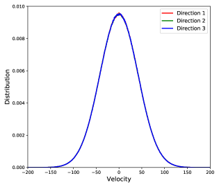
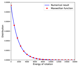
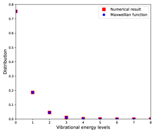
Figure 2: Top left: Distribution function of velocities at equilibrium: $x$ direction (blue), $y$ direction (red) and $z$ direction (green). Top right: Distribution of the energy of rotation: numerical result (blue) and equilibrium theoretical distribution (red). Bottom: discrete distribution of the vibrational energy: numerical result (blue) and theoretical result (red).

In figure 2, we show the distribution of velocities, rotational energy, and vibrational energy, obtained at steady state. This distributions are compared to the components of the Maxwellian distribution (19), and we observe a prefect agreement between them, which proves that the correct equilibrium is captured by the model.

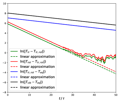
Figure 3: Relaxation of temperatures differences: $(T_{tr}-T_{tr,rot})$ (green), $(T_{rot}-T_{tr,rot})$ (red), $(T_{tr,rot}-T_{eq})$ (blue), $(T_{vib}-T_{eq})$ (black).

Now we plot in figure 3 the temperature differences $T_{tr}-T_{tr,rot}$, $T_{rot}-T_{tr,rot}$, $T_{tr,rot}-T_{eq}$, and $T_{vib}-T_{eq}$. We observe that this functions converge exponentially, as expected (even if a numerical noise is observed for $t>20\tau$ which corresponds to machine accuracy when the translational and the rotational temperatures are converged). Moreover, according to (45), the slopes of these convergence curves can be used to compute $Z_{rot}$ and $Z_{vib}$, a posteriori. We find $Z_{rot}=4.878$ and $Z_{vib}=19.61$, which is very close to the expected values.

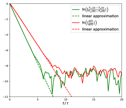
Figure 4: Relaxation of the difference of temperatures $(T_{11}-T_{tr})$ (green) and first component of the heat flux $q_{1}$ (red).

Finally, we plot in figure 4 the evolution of the difference of the first directional temperature $T_{11}$ and the mean translational temperature $T_{tr}$, as well as the evolution of the first component of the heat flux $q_{1}$. According to equation (48), it is possible to estimate the Prandtl number by evaluating the slopes of the of these quantities: we find $0.71$, which is close to the input value $0.75$.

9 Conclusion

In this paper, we have proposed an extension of the original polyatomic ES-BGK model to take into account discrete levels of vibrational energy. For a gas flow in non-equilibrium, for instance for a high enthalpy flow, we expect this model to capture the shock position and the parietal heat flux with more accuracy. This model satisfies the conservation properties and the H-theorem and allows to adjust correct transport coefficients and relaxation rates. It has been illustrated by numerical simulations for an homogeneous problem. Finally, a reduced model which also satisfies the conservation laws and the H-theorem has been obtained: with this model, it should be possible to make simulations at a computational cost which is of same order of magnitude as for a monoatomic gas.

Appendix A Inequality for $\det(\Theta)/det(\Pi)$

Here we prove the result for inequality (37) which is: $\frac{\det\Theta}{\det\Pi}\leq\left(\frac{E_{tr}(f)}{e_{tr}^{rel}}\right)^{3}$. We establish the result in a basis where $\Theta$ can be diagonalized and we note $\Theta_{1},\Theta_{2},\Theta_{3}$ its eigenvalues. Note that $\Pi$ is diagonal in the same basis. Then we have

$$\frac{\det\Theta}{\det\Pi}=\frac{\prod_{i=1}^{3}\Theta_{i}}{\prod_{i=1}^{3}(\Gamma RT_{eq}+(1-\Gamma)(\theta(RT_{tr,rot})+(1-\theta)(\nu\Theta_{i}+(1-\nu)RT_{tr})}.$$

The proof is based on convexity arguments. However, since parameter $\nu$ can be negative (we remind that $\nu$ lies in $[-\frac{1}{2},1]$), we first want to obtain an lower bound for ${\det\Pi}$ that does not depend on $\nu$.

First, we consider $\det\Pi$ as a function of $\nu$, and we take its logarithm denoted by $\phi(\nu)$:

$$\phi(\nu)=\sum_{i=1}^{3}\log(\Gamma RT_{eq}+(1-\Gamma)(\theta(RT_{tr,rot})+(1-\theta)(\nu\Theta_{i}+(1-\nu)RT_{tr}).$$

By computing their second derivatives, it can easily be seen that each component of this sum is a concave function of $\nu$, and so is the function $\phi$. Moreover, a simple derivation and relation $\sum_{i=1}^{3}\Theta_{i}=3RT_{tr}$ (see section 3.2) show that $\phi^{\prime}(0)=0$. These two properties imply that $\phi$ necessarily reaches its minimum on $[-\frac{1}{2},1]$ at $\nu=-\frac{1}{2}$ or at $\nu=1$.

Now we have to determine what is the minimum between $\phi(-\frac{1}{2})$ and $\phi(1)$. In order to simplify the notations, we introduce $X=\Gamma RT_{eq}+(1-\Gamma)\theta RT_{tr,rot}$, which is positive, and $Y=(1-\Gamma)(1-\theta)$, which is in $[0,1[$. Then we find

$$\phi(-\frac{1}{2})=\log(\prod_{i=1}^{3}(X+Y\frac{\Theta_{j}+\Theta_{k}}{2}))\quad\text{ and }\quad\phi(1)=\log(\prod_{i=1}^{3}(X+Y\Theta_{i})),$$

where $j$ and $k$ in the first expression denote the two other indices different from $i$. A convex inequality (which is nothing but the usual inequality between arithmetic and geometric means) implies

$$\phi(-\frac{1}{2})\geq\log(\prod_{i=1}^{3}(\sqrt{(X+Y\Theta_{j}}\sqrt{(X+Y\Theta_{k}}))=\log(\prod_{i=1}^{3}(X+Y\Theta_{i}))=\phi(1).$$

Consequently, $\phi(\nu)\geq\phi(1)$ for every $\nu$ in $[-\frac{1}{2},1]$: this implies $\det\Pi\geq\prod_{i=1}^{3}(X+Y\Theta_{i})$ and we deduce this upper bound

$$\frac{\det\Theta}{\det\Pi}\leq\prod_{i=1}^{3}\frac{\Theta_{i}}{X+Y\Theta_{i}},$$ (70)

that does not depend on $\nu$ anymore, as announced above.

In the last part, we analyze the logarithm of the right-hand side of the previous inequality: we denote by

$$g(\Theta)=\log\prod_{i=1}^{3}\frac{\Theta_{i}}{X+Y\Theta_{i}}=\sum_{i=1}^{3}f(\Theta_{i}),$$

where $f(s)=\log\left(\frac{s}{X+Ys}\right)$ is clearly a concave function. Then we use the Jensen inequality to get

$$\begin{split}\frac{1}{3}g(\Theta)&=\frac{1}{3}\sum_{i=1}^{3}f(\Theta_{i})\leq f\left(\frac{1}{3}\sum_{i=1}^{3}\Theta_{i}\right)\\ &=f(RT_{tr})=\log\left(\frac{RT_{tr}}{X+YRT_{tr}}\right).\end{split}$$

Now we note that $X+YRT_{tr}=RT_{tr}^{rel}$ (see the definition of $X$ and $Y$ above and the definition (28)) of $T_{tr}^{rel}$, so that $g(\Theta)\leq\log((\frac{RT_{tr}}{RT_{tr}^{rel}})^{3})$. Finally, we use this estimate in (70) to find

$$\frac{\det\Theta}{\det\Pi}\leq\left(\frac{RT_{tr}}{RT_{tr}^{rel}}\right)^{3},$$

and this gives the result, since we remind that $E_{tr}(f)=\frac{3}{2}RT_{tr}$ and $e_{tr}^{rel}=\frac{3}{2}RT_{tr}^{rel}$.

Appendix B First and second order partial derivatives of $\mathcal{S}$

We remind that

$$\mathcal{S}(e_{1},e_{2},e_{3})=R\left(\frac{3}{2}\log(e_{1})+\frac{\delta}{2}\log(e_{2})+\log\left(1+\frac{e_{3}}{RT_{0}}\right)+\frac{e_{3}}{RT_{0}}\log\left(1+\frac{RT_{0}}{e_{3}}\right)\right).$$

The first order derivatives of $S$ are

$$\partial_{1}\mathcal{S}=\frac{3}{2}R\frac{1}{e_{1}},\qquad\partial_{2}\mathcal{S}=\frac{\delta}{2}R\frac{1}{e_{2}},\qquad\partial_{3}\mathcal{S}=\frac{1}{T_{0}}\log\left(1+\frac{RT_{0}}{e_{3}}\right).$$

At $(e_{1},e_{2},e_{3})=(e_{tr}^{rel},e_{rot}^{rel},e_{vib}^{rel})$, with the corresponding definitions (25) and (28) of the relaxation temperatures, the relations above give

$$\partial_{1}\mathcal{S}=\frac{1}{T_{tr}^{rel}},\qquad\partial_{2}\mathcal{S}=\frac{1}{T_{rot}^{rel}},\qquad\partial_{3}\mathcal{S}=\frac{1}{T_{vib}^{rel}},$$

while the second order derivatives are

$$\partial_{1,1}\mathcal{S}=-\frac{3R}{2(e_{tr}^{rel})2},\qquad\partial_{2,2}\mathcal{S}=-\frac{\delta R}{2(e_{rot}^{rel})^{2}},\qquad\partial_{3,3}\mathcal{S}=-\frac{R}{e_{vib}^{rel}\left(RT_{0}+{e_{vib}^{rel}}\right)},$$

and are clearly negative, while the cross derivatives are zero.

Appendix C Second order expansion of $\Sigma(f)$ and $q(f)$

Since $\mathcal{M}[f]=\mathcal{M}_{tr}[f]\mathcal{M}_{rot}[f]\mathcal{M}_{vib}[f]$, the expansion of $\partial_{t}\mathcal{M}[f]+v\cdot\nabla\mathcal{M}[f]$ requires the expansion of the transport operator applied to each component of $\mathcal{M}[f]$. We only detail here how we proceed for the translation component $\mathcal{M}_{tr}[f]$. The chain rule gives

$$\begin{split}\partial_{t}\mathcal{M}_{tr}[f]+v\cdot\nabla\mathcal{M}_{tr}[f]=&\left[\frac{\partial_{t}\rho+v\cdot\nabla\rho}{\rho}+(\partial_{t}u+(v\cdot\nabla)u)\cdot\frac{v-u}{RT_{eq}}\right.\\ &\quad\left.+(\partial_{t}T_{eq}+v\cdot\nabla T_{eq})\left(\frac{|v-u|^{2}}{2RT_{eq}}-\frac{3}{2}\right)\frac{1}{T_{eq}}\right]\mathcal{M}_{tr}[f].\end{split}$$

Euler equations (54) are used to replace time derivatives of $\rho$, $u$, and $T_{eq}$ by their space derivatives, and finally, we use the change of variables $V=\frac{v-u}{\sqrt{RT_{eq}}}$ to get

$$\partial_{t}M_{tr}[f]+v\cdot\nabla M_{tr}[f]=\frac{\rho}{(RT_{eq})^{3/2}}M_{0}(V)\left(A(V)\cdot\frac{\nabla\theta}{\sqrt{\theta}}+B(V):\nabla u\right)+O({\rm Kn}),$$

with

$$A(V)=\left(\frac{|V|^{2}}{2}-\frac{5}{2}\right)V,\qquad\text{ and }\qquad B(V)=V\otimes V-\left(\left(\frac{|V|^{2}}{2}-\frac{3}{2}\right)C+1\right)I.$$

The same kind of algebra is also used for the components $\mathcal{M}_{rot}[f]$ and $\mathcal{M}_{vib}[f]$. They are much simpler and are left to the reader.

Appendix D Gaussian integrals and other summation formulas

In this section, we give some summation and integrals formula that are used in the paper. First, we have $\sum_{i=0}^{+\infty}e^{-i\theta}=\frac{1}{1-e^{-\theta}}$ and $\sum_{i=0}^{+\infty}ie^{-i\theta}=\frac{e^{-\theta}}{(1-e^{-\theta})^{2}}$, which can be used to obtain

$$\sum_{i=0}^{+\infty}{\cal M}_{vib}(i)[f]=1,\qquad\text{ and }\qquad\sum_{i=0}^{+\infty}iRT_{0}{\cal M}_{vib}(i)[f]=\frac{\delta_{v}(T_{eq})}{2}RT_{eq}.$$

Then, we remind the gamma function ${\bf\Gamma}(x)=\int_{0}^{+\infty}s^{x-1}e^{-s}\,ds$, which is such that ${\bf\Gamma}(x+1)=x{\bf\Gamma}(x)$ and ${\bf\Gamma}(1)=1$. This is used to get

$$\int_{0}^{+\infty}{\cal M}_{rot}[f](\varepsilon)\,d\varepsilon=1\qquad\text{ and }\qquad\int_{0}^{+\infty}\varepsilon{\cal M}_{rot}[f](\varepsilon)\,d\varepsilon=\frac{\delta}{2}RT_{eq}.$$

Finally, we remind the definition of the absolute Maxwellian $M_{0}(V)=\frac{1}{(2\pi)^{\frac{3}{2}}}\exp(-\frac{|V|^{2}}{2})$. We denote by $\langle\phi\rangle_{V}=\int_{{\mathbb{R}}^{3}}\phi(V)\,dV$ for any function $\phi$. It is standard to derive the following integral relations (see [28], for instance), written with the Einstein notation:

$$\langle M_{0}\rangle_{V}=1,$$

$$\langle V_{i}V_{j}M_{0}\rangle_{V}=\delta_{ij},\qquad\langle V_{i}^{2}M_{0}\rangle_{V}=1,\qquad\langle|V|^{2}M_{0}\rangle_{V}=3,$$

$$\langle V_{i}V_{j}V_{k}V_{l}M_{0}\rangle_{V}=\delta_{ij}\delta_{kl}+\delta_{ik}\delta_{jl}+\delta_{il}\delta_{jk},\qquad\langle V_{i}^{2}V_{j}^{2}M_{0}\rangle_{V}=1+2\,\delta_{ij}$$

$$\langle V_{i}V_{j}|V|^{2}M_{0}\rangle_{V}=5\,\delta_{ij},\qquad\langle|V|^{4}M_{0}\rangle_{V}=15,$$

$$\langle V_{i}V_{j}|V|^{4}M_{0}\rangle_{V}=35\,\delta_{ij},\qquad\langle|V|^{6}M_{0}\rangle=105,$$

while all the integrals of odd power of $V$ are zero. Note that the first relation of each line implies the other relations of the same line: these relations are given here to improve the readability of the paper. From the previous Gaussian integrals, it can be shown that for any $3\times 3$ matrix $C$, we have

$$\langle V_{i}V_{j}C_{kl}V_{k}V_{l}M_{0}\rangle_{V}=C_{ij}+C_{ji}+C_{ii}\delta_{ij}.$$

References

• [1] G. A. Bird. Molecular Gas Dynamics and the Direct Simulation of Gas Flows. Oxford Engineering Science Series, 2003.
• [2] Iain D. Boyd and Thomas E. Schwartzentruber. Nonequilibrium Gas Dynamics and Molecular Simulation. Cambridge Aerospace Series. Cambridge University Press, 2017.
• [3] E.P. Gross, P.L. Bhatnagar, and M. Krook. A model for collision processes in gases. Physical review, 94(3):511–525, 1954.
• [4] Jr. Lowell H. Holway. New statistical models for kinetic theory: Methods of construction. Physics of Fluids, 9(9):1658–1673, 1966.
• [5] E. M. Shakhov. Generalization of the Krook relaxation kinetic equation. Izv. Akad. Nauk SSSR. Mekh. Zhidk. Gaza, pages 142–145, 1968.
• [6] V. A. Rykov. A model kinetic equation for a gas with rotational degrees of freedom. Fluid Dynamics, 10(6):959–966, 1975.
• [7] P. Andries, P. Le Tallec, J.-P. Perlat, and B. Perthame. The gaussian-BGK model of boltzmann equation with small Prandtl number. Eur. J. Mech. B-Fluids, pages 813–830, 2000.
• [8] P. Jenny, M. Torrilhon, and S. Heinz. A solution algorithm for the fluid dynamic equations based on a stochastic model for molecular motion. Journal of computational physics, 229(4):1077–1098, 2010.
• [9] M.H. Gorji, M. Torrilhon, and P. Jenny. Fokker-–Planck model for computational studies of monatomic rarefied gas flows. Journal of fluid mechanics, 680:574–601, August 2011.
• [10] H. Gorji and P. Jenny. A Kinetic Model for Gas Mixtures Based on a Fokker-Planck Equation. Journal of Physics: Conference Series, 362(1):012042–, 2012.
• [11] M. H. Gorji and P. Jenny. A Fokker–Planck based kinetic model for diatomic rarefied gas flows. Physics of Fluids, 25(6):062002, 2013.
• [12] J. Mathiaud and L. Mieussens. A Fokker–Planck model of the Boltzmann equation with correct Prandtl number. Journal of Statistical Physics, 162(2):397–414, Jan 2016.
• [13] J. Mathiaud and L. Mieussens. A Fokker–Planck model of the Boltzmann equation with correct Prandtl number for polyatomic gases. Journal of Statistical Physics, 168(5):1031–1055, Sep 2017.
• [14] J. Mathiaud and L. Mieussens. Bgk and Fokker-planck models of the boltzmann equation for gases with discrete levels of vibrational energy. Journal of Statistical Physics, 178(5):1076–1095, 2020.
• [15] J. Mathiaud. Models and methods for complex flows: application to atmospheric reentry and particle / fluid interactions. Habilitation à diriger des recherches, University of Bordeaux, June 2018.
• [16] C. Baranger, Y. Dauvois, G. Marois, J. Mathe, J. Mathiaud, and L. Mieussens. A BGK model for high temperature rarefied gas flows. European Journal of Mechanics - B/Fluids, 80:1 – 12, 2020.
• [17] Behnam Rahimi and Henning Struchtrup. Capturing non-equilibrium phenomena in rarefied polyatomic gases: A high-order macroscopic model. Physics of Fluids, 26(5):052001, 2014.
• [18] Z. Wang, H. Yan, Q. Li, and K. Xu. Unified gas-kinetic scheme for diatomic molecular flow with translational, rotational, and vibrational modes. Journal of Computational Physics, 350:237 – 259, 2017.
• [19] T. Arima, T. Ruggeri, and M. Sugiyama. Rational extended thermodynamics of a rarefied polyatomic gas with molecular relaxation processes. Phys. Rev. E, 96:042143, Oct 2017.
• [20] S. Kosuge, H.-W. Kuo, and K. Aoki. A kinetic model for a polyatomic gas with temperature-dependent specific heats and its application to shock-wave structure. Journal of Statistical Physics, 177(2):209–251, Oct 2019.
• [21] J. D. Anderson. Hypersonic and high-temperature gas dynamics second edition. American Institute of Aeronautics and Astronautics, 2006.
• [22] T. F. Morse. Kinetic model for gases with internal degrees of freedom. Phys. Fluids, 7(159), 1964.
• [23] A. B. Huang and D. L. Hartley. Nonlinear rarefied couette flow with heat transfer. Phys. Fluids, 11(6):1321, 1968.
• [24] C. David Levermore. Moment closure hierarchies for kinetic theories. Journal of Statistical Physics, 83(5):1021–1065, 1996.
• [25] B. Perthame. Boltzmann type schemes for gas dynamics and the entropy property. SIAM Journal on Numerical Analysis, 27(6):1405–1421, 1990.
• [26] B. Dubroca and L. Mieussens. A conservative and entropic discrete-velocity model for rarefied polyatomic gases. ESAIM Proceedings, 10:127–139, CEMRACS 1999.
• [27] B. Lapeyre, E. Pardoux, and R. Sentis. Méthodes de Monte-Carlo pour les équations de transport et de diffusion. Mathématiques et applications. Springer, Berlin, 1998.
• [28] S. Chapman and T.G. Cowling. The mathematical theory of non-uniform gases. Cambridge University Press, 1970.
Refer to caption
Refer to caption