Partial Order Resolution of Event Logs for Process Conformance Checking

Abstract

While supporting the execution of business processes, information systems record event logs. Conformance checking relies on these logs to analyze whether the recorded behavior of a process conforms to the behavior of a normative specification. A key assumption of existing conformance checking techniques, however, is that all events are associated with timestamps that allow to infer a total order of events per process instance. Unfortunately, this assumption is often violated in practice. Due to synchronization issues, manual event recordings, or data corruption, events are only partially ordered. In this paper, we put forward the problem of partial order resolution of event logs to close this gap. It refers to the construction of a probability distribution over all possible total orders of events of an instance. To cope with the order uncertainty in real-world data, we present several estimators for this task, incorporating different notions of behavioral abstraction. Moreover, to reduce the runtime of conformance checking based on partial order resolution, we introduce an approximation method that comes with a bounded error in terms of accuracy. Our experiments with real-world and synthetic data reveal that our approach improves accuracy over the state-of-the-art considerably.

1 Introduction

The execution of business processes is these days supported by information systems [1]. Whether it is the handling of a purchase order in e-commerce, the tracking of an issue in complaint management, or monitoring of patient pathways in healthcare, information systems track the progress of processes in terms of event data. An event hereby denotes the execution of a specific activity (e.g., checking plausibility of a purchase order, proposing some issue resolution, creating a patient treatment plan) as part of a specific case (e.g., a purchase order, an issue ticket, a patient) at a specific point in time [2]. A collection of such events, referred to as an event log, therefore represents the recorded behavior of a process.

A considerable threat to process improvement initiatives is non-conformance in process execution, i.e., situations in which the actual behavior of a process deviates from the desired behavior [3]. Such differences stem from the fact that information systems support process execution, but do not enforce a particular way of executing the process [4]. Rather, human interaction drives a process, giving people a certain flexibility in the execution of a particular case. The implications of non-conformance are known to be severe. They range from reduced productivity [5] to financial penalties imposed by authorities [6]. To efficiently detect cases of non-conformance, techniques for conformance checking have been introduced [3, 7, 8]. They strive for automatic detection of deviations of the recorded and desired process behavior, by comparing event logs with process models. They verify whether the causal dependencies for activity execution, as specified in a process model, hold true in an event log and provide diagnostic information on non-conformance.

However, a key assumption of state-of-the-art conformance checking techniques is that all events of a case are labeled with timestamps that allow to infer a total order [9]. Unfortunately, this assumption is often violated. In practice, there are various sources affecting the quality of recorded event data, among them synchronization issues, manual recording of events, or unreliable data sensing [10]. For instance, in healthcare processes, only the day of a set of treatments may be known, but not the specific point in time [11]. Hence, events are only partially ordered, which renders existing conformance checking techniques inapplicable.

In this paper, we argue that it is often possible to resolve the unknown order of such events. Our idea is to use information from the entire event log to estimate the probability of each possible total order, induced by the partial order of events. This way, conformance checking is grounded in a stochastic model, incorporating the probabilities of specific order resolutions.

Our contributions and the structure of the paper, following background on conformance checking and uncertain event data in the next section, are summarized as follows:

• We introduce the problem of partial order resolution for event logs (Section 3). We formalize the problem and outline how it enables probabilistic conformance checking.

• We present various behavioral models to address partial order resolution (Section 4). These models encode different levels of abstraction of event orders, which are then used to correlate events of different cases.

• To improve the computational efficiency of conformance checking in the presence of order uncertainty, we propose a sample-based approximation method that provides statistical guarantees on obtained conformance checking results (Section 5).

• The accuracy and efficiency of our approach, as well as the approximation method are demonstrated through evaluation experiments based on real-world and synthetic data collections (Section 6). The conducted experiments reveal that our approach achieves considerably more accurate results than the state-of-the-art, reducing the average error by 59.0%.

Finally, we review our contributions in light of related work (Section 7) and conclude (Section 8).

2 Background

Section 2.1 first introduces a running example and illustrates the goal of conformance checking. Section 2.2 then discusses the impact that order uncertainty has on this task.

2.1 Conformance Checking

Conformance checking analyzes deviations between the recorded and the desired behavior of a process. Recorded behavior is given as a log of events, each event carrying at least a timestamp, a reference to an activity, and an identifier of the case for which an activity was executed. Based on the latter, a log can be partitioned into traces: ordered, maximal sets of events, all related to the same, individual case.

The desired behavior of a process, in turn, is captured by a normative specification, i.e., a process model. It defines causal dependencies for the activities of a process, thereby inducing a set of execution sequences, i.e., sequences of possible activity executions that are allowed according to the process model. Conformance checking determines whether a recorded trace corresponds to an execution sequence of the process model. Put differently, it assesses whether a trace represents a word of the language of the process model.

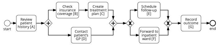
Figure 1: Process model capturing the desired behavior for a healthcare process.

For illustration, consider the process model depicted in Figure 1, henceforth referred to as model $M$. It defines the desired behavior of a healthcare process, using the Business Process Model and Notation (BPMN). That is, in each case, a patient’s history should first be reviewed (activity $A$), before checking their insurance coverage ($B$) and creating a treatment plan ($C$). In parallel, the general practitioner (GP) of the patient is contacted ($D$). Depending on the result of these activities, a patient either gets a follow-up appointment ($E$) or is forwarded to the inpatient ward ($F$), before the outcome is recorded ($G$).

Next to this process model, consider the following traces: $\pi_{1}=\langle a,b,c,d,e,g\rangle$, $\pi_{2}=\langle a,b,c,e,d,g\rangle$, and $\pi_{3}=\langle a,d,b,f,e,g\rangle$. We observe that $\pi_{1}$ represents a proper execution sequence of the process model $M$, so we can conclude that $\pi_{1}$ conforms to $M$. By contrast, $\pi_{2}$ and $\pi_{3}$ do not. In $\pi_{2}$, activity $E$ occurs before $D$. That is, a follow-up appointment was scheduled ($E$) without first contacting the patient’s GP ($D$), even though the model explicitly specifies that these activities should occur in the reverse order. Trace $\pi_{3}$ has several different issues. First, the creation of a treatment plan ($C$) has been omitted, even though this represents a mandatory activity. Second, a follow-up appointment has been scheduled ($E$), even though the patient has also been forwarded to the inpatient ward ($F$). According to the model, these activities are defined to be mutually exclusive, therefore leading to another conformance issue.

Conformance checking techniques aim to automatically detect such deviations between recorded and desired process behavior. State-of-the-art techniques for this task construct alignments between traces and execution sequences of a model to detect deviations [3, 9, 12]. An alignment is a sequence of steps, each step comprising a pair of an event and an activity, or a skip symbol $\bot$, if an event or activity is without counterpart. For instance, for the non-conforming trace $\pi_{3}$, an alignment with two such skip steps may be constructed with the execution sequence $\langle A,D,B,C,F,G\rangle$ of the model:

$$\begin{array}[]{l c c c c c c c}\text{Trace }\pi_{3}&a&d&b&\bot&f&e&g\\ \hline\cr\text{Execution sequence}&A&D&B&C&F&\bot&G\\ \end{array}$$

Assigning costs to skip steps, a cost-optimal alignment (not necessarily unique) is constructed for a trace in relation to all execution sequences of a model [9]. An optimal alignment then answers not only the question whether there are deviations between a trace and the execution sequences of a model, but also enables quantification of non-conformance by aggregating the costs of skip steps. In addition, considering a log as a whole, events and activities that are frequently part of skip steps highlight hotspots of non-conformance in process execution.

2.2 Event Data Uncertainty

While various conformance checking techniques have been presented in recent years, they all assume and require event data to have been accurately recorded. Yet, in practice, event logs are subject to diverse quality issues [10, 13, 14] along all the dimensions known to assess data quality in general [15], e.g., accuracy, timeliness, precision, completeness, and reliability.

In this work, we focus on quality issues that relate to temporal aspects of events, which are highly relevant in conformance checking. In particular, state-of-the-art conformance checking relies on discrete events that are assigned a precise timestamp. Hence, the commonly adopted notion of a trace requires all events of a single case to be totally ordered by their timestamps [9, 12]. However, this assumption is often violated in practice. Below, we illustrate potential reasons for this observation. While the respective phenomena may cause various different types of data quality issues, they particularly disturb the order of events as established through their timestamps.

1. Lack of synchronization. Event logs integrate data from various information systems. Tracing the execution in such distributed systems has to cope with unsynchronized clocks [16], making timestamps partially incomparable. Also, the logical order of events induced by timestamps may be inconsistent with the order of their recording [17].

2. Manual recording. The execution of activities is not always directly observed by information systems. Rather, people involved in process execution have to record them manually. Such manual recordings are subject to inaccuracies. For instance, it has been observed in the healthcare domain that personnel records their work solely at the end of a shift [18], rendering it impossible to determine a precise order of executed activities.

3. Data sensing. Event logs may be derived from sensed data as recorded by real-time locating systems (RTLS). Then, the construction of discrete events from raw signals is inherently uncertain and grounded in probabilistic inference [19, 20]. For instance, deriving treatment events in a hospital based on RTLS positions of patients and staff members does not yield fully accurate traces [21].

The above phenomena have in common that they result in imprecise event timestamps. In conformance checking, this leads to the particular problem of order uncertainty: The exact order in which events of a trace have occurred is not known. Consider, for instance, the events shown in Table 1, recorded for a single case of the aforementioned process. The events may have been captured manually, so that the timestamps only indicate the rough hour in which activities have been executed. Since events $b$ and $c$ carry the same timestamp, it is unclear whether the patient’s insurance was checked ($B$) before or after creating a treatment plan ($C$). Since the type of insurance may influence the treatment plan, the model in Figure 1 defines an explicit execution order for both activities. Yet, due to order uncertainty, we cannot establish whether the process was indeed executed as specified.

A result of order uncertainty, whether caused by a lack of synchronization, manual recording, or data sensing issues, is that the events of a trace are only partially ordered. Such a partial order is visualized in Figure 2 for the events of the example case. This partial order induces four totally ordered sequences of events, denoted as $\pi_{4}$ to $\pi_{7}$ in the figure. Such a situation is highly problematic in conformance checking, because of the implied ambiguity. For the example in Table 1, only one of the totally ordered event sequences, i.e., $\pi_{4}$ conforms to model $M$, whereas different kinds of deviations are detected for the remaining three. Hence, one cannot conclude if the case was executed as specified by the model at all and, if it was not, which conformance violations actually occurred.

Without further insights into the execution of a case, two approaches may be followed to resolve order uncertainty. First, one may consider all induced totally ordered traces to be equally likely, so that the number of such traces that conform to the model provides a conformance measure. Second, order uncertainty may be neglected, verifying whether one of the induced total orders is conforming [18]. As we will demonstrate empirically, both approaches introduce a severe bias in conformance checking. In this work, we therefore strive for a fine-granular assessment of each induced total event order.

Table 1: Events recorded for a single case.

Event ID	Activity	Timestamp
a	Review patient history [A]	13:00
b	Check insurance coverage [B]	14:00
c	Create treatment plan [C]	14:00
f	Forward to inpatient ward [F]	15:00
d	Contact patient’s GP [D]	15:00
g	Record outcome [G]	16:00

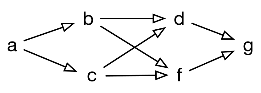
. $\pi_{4}=\langle a,b,c,d,f,g\rangle$
$\pi_{5}=\langle a,c,b,d,f,g\rangle$
$\pi_{6}=\langle a,b,c,f,d,g\rangle$
$\pi_{7}=\langle a,c,b,f,d,g\rangle$

Figure 2: Partial order and trace resolutions resulting from the order uncertainty in the case of Table 1.

3 Problem Statement

We first give preliminaries in terms of a formal model (Section 3.1), before defining the problem addressed in this paper, partial-order resolution (Section 3.2).

3.1 Preliminaries

In this section, we introduce our formal model to capture normative and recorded process behavior.

Normative process behavior. A process model defines the execution dependencies between the activities of a process, establishing the normative or desired behavior. For our purposes, it is sufficient to abstract from specific process modeling languages (e.g., BPMN or Petri nets) and focus on the behavior defined by a model. Process models capture relations that exist among a collection of activities. We denote the universe of such activities as $\mathcal{A}$. Then, a process model defines a set of execution sequences, $M\subseteq\mathcal{A}^{*}$, that capture sequences of activity executions that lead the process to its final state. For instance, the model in Figure 1 defines a total of six allowed execution sequences, including $\langle A,B,C,D,E,G\rangle$, $\langle A,B,C,D,E,F\rangle$, as well as variations in which activity $D$ occurs before or after $B$.

Recorded process behavior. The executions of activities of a process are recorded as events. If these activity executions happen within the context of a single case, the respective events are part of the same trace. While most models define traces as sequences of events, we adopt a model that explicitly captures order uncertainty by allowing multiple events, even if belonging to the same trace, to be assigned the same timestamp. Hence, the events of a trace are only partially ordered. We capture this by modeling traces as sequences of sets of events, where each set contains events with identical timestamps. Captured as follows:

Definition 1 (Traces)

A trace is a sequence of disjoint sets of events, $\sigma=\langle E_{1},\dots,E_{n}\rangle$, with $E_{\sigma}=\bigcup_{1\leq i\leq n}E_{i}$ as the set of all events of $\sigma$.

For a trace $\sigma=\langle E_{1},\dots,E_{n}\rangle$, we refer to $E_{i}$, $1\leq i\leq n$, as an event set of $\sigma$. This event set is uncertain, if $|E_{i}|>1$. Accordingly, a trace that does not contain uncertain event sets is certain, otherwise it is uncertain. Intuitively, in a certain trace, a total order of events is established by the events’ timestamps. For an uncertain trace, events within an uncertain event set are not ordered.

An event log is a set of traces, capturing the events as they have been recorded during process execution. Moreover, for each event, we capture the activity for which the execution is represented by this event. The latter establishes a link between an event log and the activities of a process model.

Definition 2 (Event Log)

An event log is a tuple $L=(\Sigma,\lambda)$, where $\Sigma$ is a set of traces and $\lambda:\bigcup_{\sigma\in\Sigma}E_{\sigma}\rightarrow\mathcal{A}$ assigns activities to all events of all traces.

As a short-hand notation, we write a trace of a log not only as a sequence of sets of events, but also as a sequence of sets of activities. That is, for a trace $\langle\{e_{1},e_{2}\},\{e_{3}\}\rangle$ with $\lambda(e_{1})=x$, $\lambda(e_{2})=y$, and $\lambda(e_{3})=z$, we also write $\langle\{x,y\},\{z\}\rangle$. According to this model, the case from Table 1 is captured by the trace $\sigma_{1}=\langle\{a\},\{b,c\},\{d,f\},\{g\}\rangle$.

3.2 The Partial Order Resolution Problem

To assess the conformance of an event log with a model, the order uncertainty of its traces needs to be handled. Yet, there may be several ways to resolve this uncertainty as the events of each uncertain event set may be ordered differently. We capture such different orders by means of possible resolutions of event sets and, based thereon, of a trace.

Definition 3 (Possible Resolutions)

Given a trace $\sigma=\langle E_{1},\dots,E_{n}\rangle$, we define possible resolutions for:

• an event set $E_{i}$, as any total order over its events, i.e., $\Phi(E_{i})=\{\langle e_{1},\ldots,e_{|E_{i}|}\rangle\mid\forall\ 1\leq j,k\leq|E_{i}|:e_{j}~{}\in~{}E_{i}\ \wedge\ e_{j}=e_{k}\Rightarrow j=k\}$;

• the trace $\sigma$, as any total order over events of its event sets, i.e., $\Phi(\sigma)=\{\langle e^{1}_{1},\ldots,e^{m_{1}}_{1},\ldots,e^{1}_{n},\ldots e^{m_{n}}_{n}\rangle\mid\forall\ 1\leq i\leq n:\langle e^{1}_{i},\ldots e^{m_{i}}_{i}\rangle\in\Phi(E_{i})\}$.

In the context of an event log $L=(\Sigma,\lambda)$, we lift the short-hand notation for traces based on the assigned activities to resolutions. Then, for our example trace $\sigma_{1}=\langle\{a\},\{b,c\},\{d,f,\},\{g\}\rangle$, possible resolutions would be $\langle a,c,b,f,d,g\rangle$ or $\langle a,b,c,d,f,g\rangle$, but neither $\langle a,b,f,d,g\rangle$ (event $c$ is missing) nor $\langle a,c,f,b,d,g\rangle$ (events from different event sets are interleaved).

Although the events originally occurred in a total order, there is no way to recover this original order when it is obscured due to the aforementioned reasons for order uncertainty. However, we argue that even without identifying a single resolution, valuable insights on the conformance of a trace may be obtained. This can be achieved by assessing which resolutions of a trace conform and which do not conform to a process model. As illustrated above, it is crucial here to avoid basing conformance assessments purely on the number of possible resolutions that conform to its associated process model: a single conforming resolution may be more likely to have occurred than multiple non-conforming resolutions combined.

We therefore resort to a probabilistic model that defines a probability distribution over a trace’s possible resolutions. Then, conformance checking can be grounded in the cumulative probabilities of the resolutions that conform to a model, or show particular deviations, respectively. Following this line, a crucial problem addressed in this paper is how to assign probabilities to the possible resolutions of a partial order, which can be phrased as follows:

Problem 1 (Partial Order Resolution)

Let $L=(\Sigma,\lambda)$ be an event log. The partial order resolution problem is to derive, for each trace $\sigma\in\Sigma$ and each possible resolution $\varphi\in\Phi(\sigma)$, the probability $P(\varphi)$ of $\varphi$ representing the order of event generation for the respective case.

Based on the probabilities $P(\varphi)$ of each resolution $\varphi\in\Phi(\sigma)$, the probabilistic conformance of a trace $\sigma$ with respect to a model $M$ can be assessed. Let $\mathit{conf}(\varphi,M)$ be a function that quantifies the conformance of a resolution to model $M$. Exemplary functions are a binary function $\mathit{conf}_{\mathit{bin}}:\varphi\times M\rightarrow\{0,1\}$, indicating a conforming resolution with 1 and a non-conforming with 0, or a function based on trace fitness [3], yielding a range from 0 to 1, i.e., $\mathit{conf}_{\mathit{fit}}:\varphi\times M\rightarrow[0,1]$. Based on such a function, the weighted conformance of a trace is denoted as follows:

$$\mathit{P_{\mathit{conf}}}(\sigma,M)=\sum_{\varphi\in\Phi(\sigma)}P(\varphi)\times\mathit{conf}(\varphi,M)$$ (1)

Similarly, more fine-granular feedback based on non-conformance may be given by analyzing alignments obtained per possible resolution of a trace. For instance, the probabilities assigned to resolutions can be incorporated as weighting factors in the aggregation of the non-conformance measured per possible resolution. This manifests itself in the form of the accumulative probabilities associated with the skip steps ($\bot$) in an alignment, as shown in Section 2.1. In this way, probabilistic conformance checking can be used to identify hotspots of non-conformance in processes.

4 Partial Order Resolution

To estimate the probability of a partial order resolution, we follow the idea that the context of a trace provided by the event log is beneficial. A business process is structured through the causal dependencies for the execution of activities. These dependencies are manifested in the traces in terms of behavioral regularities. Assuming that order uncertainty occurs independently of the execution of the process, behavioral regularities among the traces may be exploited for partial order resolution. The probability of a specific resolution for a given trace may be assessed based on order information derived from similar traces contained in the event log. Intuitively, if one possible resolution denotes an order of activity executions that is frequently observed for other traces, this resolution is expected to be more likely than another resolution that denotes a rare execution sequence. It is important to note that model characteristics cannot be leveraged to determine the likelihood of a resolution since this would introduce a bias towards conforming resolutions.

Using traces for partial order resolution requires a careful selection of the abstraction level based on which traces are compared. In practice, event logs contain traces encoding a large number of different sequences of activity executions. Reasons for that are concurrent execution of activities, which leads to an exponential blow-up of the number of execution sequences, as well as the presence of noise, such as incorrectly recorded events. For a possible resolution of a trace, it may therefore be impossible to observe the exact same sequence of activity executions in another trace, unaffected by order uncertainty. We cope with this issue by defining behavioral models that realize different levels of abstraction in the comparison of traces. We propose (i) the trace equivalence model, (ii) the N-gram model, and (iii) the weak order model, see Table 2. The models differ in the notion of behavioral regularity that is used for the partial order resolution.

Table 2: Proposed behavioral models.

Model	Illustration	Basis
Trace equivalence		Equal, certain traces
N-gram		Equal sub-sequences of length $N$
Weak order		Indirectly follows relation of events

4.1 Trace Equivalence Model

This model estimates the probability of a resolution by exploring how often the respective sequence of activity executions is observed in the event log, in traces without order uncertainty. To this end, we first clarify that two resolutions shall be considered to be equivalent, if they represent the same sequences of executed activities.

Let $L=(\Sigma,\lambda)$ be an event log and $\sigma,\sigma^{\prime}\in\Sigma$ two traces of the same length, i.e., $|E_{\sigma}|=|E_{\sigma^{\prime}}|$. Let $\varphi=\langle e_{1},\ldots,e_{n}\rangle\in\Phi(\sigma)$ and $\varphi^{\prime}=\langle e^{\prime}_{1},\ldots,e^{\prime}_{n}\rangle\in\Phi(\sigma^{\prime})$ two of their resolutions. Then, the resolutions are equivalent, denoted by $\varphi\equiv\varphi^{\prime}$, if and only if $\lambda(e_{i})=\lambda(e^{\prime}_{i})$ for $1\leq i\leq n$.

We define $\Sigma_{certain}=\{\sigma\in\Sigma\mid|\Phi(\sigma)|=1\}$ as the set of all certain traces, i.e., all traces that do not have uncertainty and, thus, only a single resolution. Then, we quantify the probability associated with a resolution $\varphi\in\Phi(\sigma)$ of a trace $\sigma$ as the fraction of certain traces for which the resolutions are equivalent:

$$P_{trace}(\varphi)=\frac{\left|\left\{\sigma\in\Sigma_{certain}\mid\exists\ \varphi^{\prime}\in\Phi(\sigma):\varphi^{\prime}\equiv\varphi\right\}\right|}{|\Sigma_{certain}|}$$ (2)

The above model enables a direct assessment of the probability of a resolution. Yet, it may have limited applicability: (i) It only considers certain traces, and there may only be a small number of those in a log; (ii) none of the certain traces may show an equivalent resolution, as it requires the entire sequence of activity executions to be the same.

4.2 N-Gram Model

As a second approach, we introduce a behavioral model based on N-gram approximation. It takes up the idea of sequence approximations as they are employed in a broad range of applications, such as prediction [22] and speech recognition [23]. Specifically, N-gram approximation enables us to define a more abstract notion of behavioral regularities that determines which traces shall be considered when computing the probability of a resolution.

Given a resolution of a trace, this model first estimates the probability of the individual events of the resolution occurring at their specific position. Here, up to $N-1$ events preceding the respective event are considered and their probability of being followed by the event in question is determined. The latter is based on all traces of the log that comprise sub-sequences of the same activity executions without order uncertainty. For instance, for $N=4$ and a resolution $\varphi_{1}=\langle a,b,c,d,f,g\rangle$, we determine the likelihood that event $f$ occurs at the fifth position by exploring the likelihood that a sequence $\langle b,c,d\rangle$ is followed by $f$. This estimation is based on all traces of the log that comprise events of the sequence $\langle b,c,d,f\rangle$ without order uncertainty.

To formalize this idea, we first define a predicate certain. Given a log $L=(\Sigma,\lambda)$, this predicates holds for a sequence of activities $\langle a_{1},\ldots,a_{m}\rangle$, $a_{i}\in\mathcal{A}$ for $1\leq i\leq m$ and a trace $\sigma=\langle E_{1},\ldots,E_{n}\rangle\in\Sigma$, $m\leq n$, if $\sigma$ contains events for the respective activity executions without order uncertainty:

$$\begin{split}certain(\langle a_{1},\ldots,a_{m}\rangle,\sigma=\langle E_{1},\ldots,E_{n}\rangle)\Leftrightarrow&\\ \exists\ i\in\{0,\ldots,n-m\},\forall\ j\in\{1,\ldots,m\}:E_{i+j}=\{e_{i+j}&\}\wedge\lambda(e_{i+j})=a_{j}.\\ \end{split}$$ (3)

Using this predicate, we define the probability of events related to activity $a$ to follow events denoting the execution of some activities $\langle a_{1},\dots,a_{m}\rangle$. This definition is based on the number of times the two respective sequences, with and without $a$, are observed in the traces of the event log:

$$P(a\mid\langle a_{1},\dots,a_{m}\rangle)=\frac{\left|\left\{\sigma\in\Sigma\mid certain(\langle a_{1},\dots,a_{m},a\rangle,\sigma)\right\}\right|}{\left|\left\{\sigma\in\Sigma\mid certain(\langle a_{1},\dots,a_{m}\rangle,\sigma)\right\}\right|}.$$ (4)

For illustration, we return to the example of estimating the probability of events related to $f$ to be preceded by those representing the execution of activities $\langle b,c,d\rangle$. That is, we divide the number of occurrences of $\langle b,c,d,f\rangle$ by the number of occurrences of $\langle b,c,d\rangle$, while considering only traces that do not show order uncertainty for the respective events. Based thereon, the probability of a resolution is derived by aggregating the N-gram-based probabilities of all its events:

$$P_{N\text{-}gram}(\varphi=\langle e_{1},\dots e_{n}\rangle)=\prod\limits_{k=2}^{n}P(\lambda(e_{k})\mid\langle\lambda(e_{\max(1,k-N+1)}),\dots,\lambda(e_{k-1})\rangle)$$ (5)

The above approach may be adapted to explicitly consider the first events of traces in the assessment. Technically, an artificial event is added to the beginning of all traces, so that it will be part of the respective N-gram definitions. For instance, the example trace $\sigma_{1}=\langle\{a\},\{b,c\},\{d,f,\},\{g\}\rangle$ would be changed to $\sigma^{\prime}_{1}=\langle\{\circ\},\{a\},\{b,c\},\{d,f,\},\{g\}\rangle$ with $\circ$ denoting the start of the trace. Then, the estimation of the probability for the resolution $\varphi^{\prime}_{1}=\langle\circ,a,b,c,d,f,g\rangle$ would, using $N=4$, be based on an assessment of the probability that $c$ is preceded by $\langle\circ,a,b\rangle$. This explicitly considers solely traces that start with events that denote executions of $a$ and $b$.

Compared to the trace equivalence model, the N-gram model is more abstract. This makes the model more generally applicable, as it requires only the presence of traces that show equivalent sub-sequences of activity executions without order uncertainty, instead of requiring fully equivalent traces without order uncertainty. This is particularly useful to identify local dependencies that are independent of other choices in a process. For example, looking back at the running example of Figure 1, a 2-gram model would clearly be able to learn the ordering dependency between checking a patient’s insurance coverage (activity $B$) and establishing a treatment plan ($C$). However, this probability would not be dependent on whether activity $C$ is eventually followed by scheduling a follow-up ($E$) or by forwarding a patient ($F$). As such, the N-gram model would be able to identify this order requirement while imposing fewer requirements on the available data than the trace equivalence model. The parameter $N$, furthermore, provides further flexibility. Higher values of $N$ lead to longer sub-sequences being considered, which induces a stricter notion of behavioral regularities to be exploited in partial order resolution. Lower values, in turn, decrease this strictness, thereby increasing the amount of evidence on which the resolution is based.

Yet, the N-gram model assumes that behavioral regularities materialize in the form of consecutive activity executions. Even if $N=2$, only events that (certainly) follow upon each other directly in a trace are considered in the assessment.

4.3 Weak Order Model

To obtain an even more abstract model, we drop the assumption that behavioral regularities relate solely to consecutive executions of activities. Rather, indirect order dependencies, referred to as a weak order, among the activity executions, and thus events, are exploited.

To illustrate this idea, consider two resolutions, $\varphi_{1}=\langle a,b,c,d,f,g\rangle$ and $\varphi_{2}=\langle a,c,b,d,f,g\rangle$, of our example trace $\sigma_{1}$. To estimate their probabilities, under a weak order model, we determine the fraction of traces in which an event related to activity $b$ occurs at some point before $c$, or vice versa, to obtain evidence about the most likely order. Assume that the event log also contains an uncertain trace $\sigma_{2}=\langle\{a,b\},\{d\},\{c\},\{f,g\}\rangle$. In this trace, $b$ and $c$ are not part of consecutive event sets, and $b$ is even part of an uncertain event set. Still, this trace provides evidence that activity $b$ is executed before $c$, which supports resolution $\varphi_{1}$ of trace $\sigma_{1}$. Thereby, the weak order model would appropriately gain evidence that a patient’s insurance coverage should be checked ($b$) before establishing a treatment plan ($c$). Similarly, this model enables us to incorporate information from consecutive uncertain event sets, as in $\sigma_{1}=\langle\{a\},\{b,c\},\{d,f\},\{g\}\rangle$. Due to order uncertainty, it is unclear whether events $c$ and $f$ directly followed each other. However, $c$ definitely occurred earlier than $f$, i.e., a treatment plan was certainly created ($c$) before forwarding the patient to an inpatient ward ($f$). Such information would not be taken into account by the N-gram model.

Formally, let $L=(\Sigma,\lambda)$ be an event log and $a,a^{\prime}\in\mathcal{A}$ two activities. We define a predicate order to capture whether a trace comprises events representing the executions of these activities in weak order:

$$order(a,a^{\prime},\sigma=\langle E_{1},\ldots,E_{n}\rangle)\Leftrightarrow\exists\ i,j\in\{1,\ldots,n\},i<j:e_{i}\in E_{i}\wedge e_{j}\in E_{j}\wedge\lambda(e_{i})=a\wedge\lambda(e_{j})=a^{\prime}.\\$$ (6)

This predicate enables us to estimate the probability of having events related to specific activity executions in weak order. More specifically, we determine the ratio of traces that contain the respective events:

$$P(a,a^{\prime})=\frac{|\{\sigma\in\Sigma\mid order(a,a^{\prime},\sigma)\}|}{|\{\sigma\in\Sigma\mid\exists\ e,e^{\prime}\in E_{\sigma}:\lambda(e)=a\wedge\lambda(e^{\prime})=a^{\prime}\}|}.$$ (7)

Based thereon, the probability of a resolution is defined by aggregating the probabilities of all pairs of events to occur in the particular order:

$$P_{WO}(\varphi=\langle e_{1},\dots e_{n}\rangle)=\prod\limits_{\begin{subarray}{c}1\leq i<n\\ i<j\leq n\end{subarray}}P(\lambda(e_{i}),\lambda(e_{j})).$$ (8)

Compared to the other two models, the weak order model employs the most abstract notion of behavioral regularity when resolving partial orders. Consequently, the computation of the probability of a particular resolution can exploit information from many traces of an event log.

5 Result Approximation

A key issue hindering the applicability of conformance checking techniques in industry is their computational complexity, since state-of-the-art algorithms suffer from an exponential runtime complexity in the size of the process model and the length of the trace [3]. In the context of this paper, this is particularly problematic: Order uncertainty exponentially increases the number of conformance checks that are required per trace. To increase the applicability of conformance checking under order uncertainty, this section therefore proposes an approximation method incorporating statistical guarantees.

This section discusses the calculation of expected conformance values (Section 5.1) and associated confidence intervals (Section 5.2), before describing approximation method itself (Section 5.3).

5.1 Expected Conformance

To reduce the computational complexity of the conformance checking task, we propose an approximation method that provides statistical guarantees about the conformance results $P_{\mathit{conf}}(\sigma,M)$ obtained for a trace $\sigma$. The method provides a confidence interval for the conformance results, which is computed based on conformance checks performed for a sample of its possible resolutions $\Phi(\sigma)$. We use $\bar{\Phi}\subseteq\Phi(\sigma)$ to denote this sample and $\bar{p}=\sum_{\varphi\in\bar{\Phi}}P(\varphi)$ to denote the cumulative probability of the resolutions in the sample. Then, we define the expected conformance for a trace $\sigma$ to a process model $M$ as follows:

$$E(P_{\mathit{conf}}(\sigma,M))=\sum_{\varphi\in\bar{\Phi}}P(\varphi)\times\mathit{\mathit{conf}}(\varphi,M)+(1-\bar{p})\times\mu_{\mathit{conf}}$$ (9)

Equation 9 consists of two components: (i) the known, weighted conformance of the sampled resolutions, i.e., $\sum_{\varphi\in\bar{\Phi}}P(\varphi)\times\mathit{conf}(\varphi,M)$, and (ii) an estimated part, $(1-\bar{p})\times\mu_{conf}$. This estimated part receives a weight of $1-\bar{p}$, i.e., the cumulative probability of the traces not included in the sample. The estimate itself, i.e., $\mu_{\mathit{conf}}$, reflects the expected conformance of a previously unseen resolution. This value is obtained by fitting a statistical distribution over the conformance values obtained for the sample $\bar{\Phi}$. Consider the conformance functions discussed in Section 3.2: For a binary function $\mathit{conf}_{\mathit{bin}}$ with range $\{0,1\}$, the results of a sample represent a Binomial distribution. For a more fine-granular function $\mathit{conf}_{\mathit{fit}}$ based on trace fitness with range $[0,1]$, the resulting distribution can be characterized using a normal distribution for a sufficiently large sample (e.g., size over 20) following the central limit theorem [24].

For illustration, consider a sample $\bar{\Phi}$ that contains 30 resolutions, 21 conforming and 9 non-conforming. Then, the estimated, binary conformance of unseen resolutions is given as $\mu_{\mathit{conf}}=0.70$. With a cumulative probability of $\bar{p}=0.80$, the estimated component of Equation 9 equals $(1-0.80)\times 0.70=0.14$. Note that determining the expected conformance $\mu_{\mathit{conf}}$ is independent of the probabilities assigned by a behavioral model. Therefore, due to differences among the probabilities associated with the resolutions in $\bar{\Phi}$, it does not necessarily hold that $E(P_{\mathit{conf}}(\sigma,M))=\mu_{\mathit{conf}}$. For instance, for the given example, we may have $\sum_{\varphi\in\bar{\Phi}}P(\varphi)\times\mathit{\mathit{conf}}(\varphi,M)=0.60$, yielding an estimated overall conformance of $0.60+0.14=0.74$, which is considerably higher than $\mu_{\mathit{conf}}$.

5.2 Confidence Intervals

Based on statistical distributions established for expected conformance values, we further derive statistical bounds in the form of a confidence interval for the estimation of $P_{\mathit{conf}}(\sigma,M)$. Recognizing that one part of the conformance checking results is known, whereas the other requires estimation, we define the confidence interval as follows:

$$CI_{\alpha}=E(P_{\mathit{conf}}(\sigma,M))\pm(1-\bar{p})\times m_{\alpha}$$ (10)

Equation 10 consists of two components: (i) the expected conformance $E(P_{\mathit{conf}}(\sigma,M))$, and (ii) a margin, $\pm(1-\bar{p})\times m_{\alpha}$, which determines the size of the interval. Here, $m_{\alpha}$ denotes the margin of error of the distribution for a significance level $\alpha$. The margin of error for a Binomial distribution obtained over a set of binary conformance assessments, $m_{\alpha}$ is computed using, e.g., the Wilson score interval [25]. For a normal distribution, the margin of error is based on the standard error [26].

It is important to note that the width of a confidence interval established using Equation 10 decreases if the cumulative probability of the sample ($\bar{p}$) is higher. This property naturally follows, because the margin of error $m_{\alpha}$ is only applicable to the estimated component of a conformance assessment, which has the weight $1-\bar{p}$. We utilize this property in the method described next.

5.3 Computation Method

Our proposed method for efficient conformance approximation is presented in Algorithm 1. The approximation is an iterative procedure that incorporates the conformance of newly sampled resolutions until a sufficiently accurate conformance value is established.

Algorithm 1 Statistical conformance approximation method

1:input $\sigma$, a trace; $M$, a process model; $B$, a behavioral model; $\mathit{conf}$, a conformance

2:input function; $\alpha$, a significance level; $\delta$, a desired accuracy threshold.

3:$\bar{\Phi}\leftarrow\emptyset$ $\triangleright$ The set of sampled resolutions

4:$R\leftarrow[\,]$ $\triangleright$ Bag of conformance results

5:$\bar{p}\leftarrow 0$ $\triangleright$ Accumulated probability of sampled resolutions

6:repeat

7:    $\varphi\leftarrow\mathit{select}(\Phi(\sigma)\setminus\bar{\Phi},B)$ $\triangleright$ Sample a new resolution

8:    $\bar{\Phi}\leftarrow\bar{\Phi}\cup\{\varphi\}$ $\triangleright$ Add resolution to sample

9:    $R\leftarrow R\uplus[\mathit{conf}(\varphi,M)]$ $\triangleright$ Compute and add conf. result

10:    $\mathcal{D}\leftarrow\mathit{fit}(R)$ $\triangleright$ Fit distribution on the results

11:    $E\leftarrow\mathit{estimateResult}(R,\mathcal{D})$ $\triangleright$ Use Equation 9

12:    $m_{\alpha}\leftarrow\mathit{computeMargin}(\mathcal{D,\alpha})$ $\triangleright$ Margin of error

13:    $\bar{p}\leftarrow\bar{p}+P_{B}(\phi)$ $\triangleright$ Increase accumulated probability

14:until $(1-\bar{p})\times m_{\alpha}/E\leq\delta$ $\triangleright$ Check threshold

15:return $E\pm m_{\alpha}$ $\triangleright$ Return confidence interval

Loop. Each iteration starts by selecting a resolution $\phi$, which has a maximal likelihood from those in $\Phi(\sigma)\setminus\bar{\Phi}$ (line 7). This selection is guided by one of the behavioral models introduced in Section 4, as configured by the input parameter $B$. Next, the algorithm computes the conformance result for $\phi$ and adds it to $R$, the bag of conformance results (line 9). Then, statistical distribution is fit to the results sample (line 10). Based on this distribution, the estimated result is computed using Equation 9 (line 11), before the margin of error is determined (line 12) and the accumulated probability of all sampled resolutions is updated (line 13).

Stop condition. The iterative procedure is repeated until the margin of error leads to results that are below a user-specified precision threshold $\delta$. In particular, the method samples resolutions until the ratio of the margin of error $m_{\alpha}$ and the estimated conformance $E$, weighted by the complement of the accumulated probability of sampled resolutions, is below $\delta$ (line 14). The stop condition is based on the ratio, rather than the absolute margin of error, given that, for instance, a margin of $0.05$ has a considerably greater impact when $E=0.2$ than compared to $E=0.8$.

By employing this approximation method, we obtain results that satisfy a desired significance value $\alpha$ and precision level $\delta$. This means that, when possible, the method requires only a relatively low number of resolutions, whereas for traces with a higher variability among its resolutions, the method will use a greater sample to ensure result accuracy.

6 Evaluation

This section describes evaluation experiments in which we assess the accuracy of the proposed behavioral models for conformance checking. We achieve this by comparing the conformance checking results obtained for uncertain traces to the conformance results that would have been obtained without order uncertainty. These results are also compared against two baselines. Both the datasets and the implementation used to conduct these experiments are publicly available.

6.1 Data

We conducted our evaluation based on both real-world and synthetic data collections.

Real-world collection. We used three, publicly available, real-world events logs, detailed in Table 3. As shown in the table, the three logs differ considerably, for instance in terms of their size (13,087 for BPI-12 to 150,370 traces for the traffic fines log) and trace length (averages from 3.7 to 20.0 events per trace). These logs also demonstrate the prevalence of coarse-grained timestamps in real-world settings, since all logs contain a considerable amount of uncertain traces, ranging up to 93.4% of the traces for the BPI-14 log. To obtain a process model that serves as a basis for conformance checking, we use the inductive miner [27], a state-of-the-art process discovery technique, with the default parameter setting (i.e., a noise filtering threshold of 80%).

Table 3: Characteristics of the real-world collection.

Characteristic	BPI-12 [28]	BPI-14 [29]	Traffic fines [30]
Places	32	27	23
Transitions	45	29	26
Traces	13,087	41,353	150,370
Variants	4,366	31,725	231
Trace length (avg.)	20.0	7.3	3.7
Uncertain traces	5,006 (38.3%)	38,649 (93.4%)	9,166 (6.1%)
Events	262,200	369,485	561,470
Events in uncertain event sets	25,369 (9.7%)	224,515 (60.7%)	21,308 (3.8%)
Resolutions..(avg.)	21.8	91.7	3.2
Resolutions (max.)	3,072	4,608	12

Synthetic collection. We have generated a collection of 500 synthetic models with varying characteristics, including aspects such as loops, arbitrary skips, and non-free choice constructs. By using synthetic logs, we are able to assess the impact of factors such as the degree of non-conformance and order uncertainty on the conformance checking accuracy of our approach. We employed the state-of-the-art process model generation technique from [31] due to its ability to also generate non-structured models, e.g., models that include non-local decisions. To generate models, we employed the default parameters set by the technique’s developers.

For each of these models, we used a stochastic simulation plug-in of the ProM 6 framework [32] to generate an event log consisting of 1000 traces, using the default plug-in settings (i.e., uniform probabilities for all choices and exponential inter-arrival and execution times). The main characteristics of these models and their logs are detailed in Table 4.

To introduce non-conformance, we insert noise using the same simulation plug-in, which randomly inserts, swaps, and removes events in a specified fraction of the traces. For each model, we created logs with four different noise levels, by inserting noise into 25%, 50%, 75%, and 100% of the traces. This results in four sets of logs with, on average 353.8, 564.0, 774.2 and 998.4 non-conforming traces, respectively. We introduced ordering uncertainty by abstracting all timestamps to minutes, i.e., by omitting all information on seconds and milliseconds. As a result, about 50.6% of the traces in the event logs have some order uncertainty in the form of at least two unordered events. The uncertain traces have an average of 4.0 possible resolutions per trace, up to a maximum of 16,384.

Table 4: Characteristics of the synthetic collection.

Per process model				Per event log
Node Type	Avg.	Max.		Characteristic	Avg.	Max.
Places	19.1	77		Traces	1,000.0	1,000
Transitions	19.2	84		Trace length	6.4	122
And-splits	4.8	54		Uncertain traces	506.4	873
Xor-splits	3.4	28		Events in uncertain event sets	20.1%	68.7%
Silent steps	6.9	64		Resolutions	4.0	16,384

The model-log pairs included in the real-world and synthetic collections differ considerably in terms of model complexity, trace length, degree of non-conformance, and degree of uncertainty. As a result, these collections enable us to assess the impact of such key factors on the conformance checking accuracy and efficiency of our proposed behavioral models and approximation method. In this way, we make sure the experimental results have a sufficiently high level of external validity.

6.2 Setup

To conduct our evaluation experiments, we implemented the proposed approach as a plug-in for the Java-based open-source Process Mining Framework ProM 6.

Behavioral Models. Using the implementation and the datasets described above, we conducted experiments with the following behavioral models:

• TE: The trace equivalence model from Section 4.1.

• 2G, 3G, 4G: The N-gram model from Section 4.2, using $N=2$ (the strictest notion), $N=3$, and $N=4$, respectively.

• WO: The weak order model from Section 4.3.

Note that when a behavioral model returns a probability of zero for all possible resolutions of a trace, which happens if the model cannot derive any evidence from the event log, we regard all resolutions to be equally likely. That is, we assign a uniform probability $|\Phi(\sigma)|^{-1}$ to each resolution.

Approximation methods. To evaluate the impact of our proposed method for result approximation, we compute results based on two configurations:

• No approximation: the conformance for all resolutions with a non-zero probability is assessed.

• $\alpha$=0.99 approximation: the approximation method from Section 5 with $\alpha=0.99$ and $\delta=0.10$.

Performance measures. To determine how accurate the obtained conformance values are, we compare them to the true conformance values, i.e., a gold standard value, based on the order in which a trace’s events appear in a log. For the purposes of this evaluation, we consider conformance in terms of (weighted) fitness, as defined in Section 3.2. We consider accuracy at both the trace- and the log-levels, where the former focuses on the accuracy for individual traces and the latter on the accuracy obtained per log.

At the trace-level, we quantify the difference between obtained and true fitness values by employing the Root-Mean Squared Error (RMSE). Given an event log $L$, a process model $M$, and a behavioral model $B$, the RMSE is given as follows:

$$\mathit{error_{tracelevel}}(L,M,B)=\sqrt{\frac{\sum_{\sigma\in L\setminus\Sigma_{certain}}(\mathit{fit}(\sigma,M)-P_{\mathit{fit}}^{B}(\sigma,M))^{2}}{|L\setminus\Sigma_{certain}|}}$$ (11)

At the log-level, we quantify the difference between the obtained and true fitness values by computing the absolute difference:

$$\mathit{error_{loglevel}}(L,M,B)=|\mathit{fit}(L,M)-P_{\mathit{fit}}^{B}(L,M)|$$ (12)

Note that, as shown, the trace-level results are computed over only the traces with uncertainty, i.e., $L\setminus\Sigma_{certain}$, whereas the log-level results are computed over all traces in $L$.

Baselines. As a basis for comparison, we employ two baseline techniques, BL1 and BL2:

• BL1: This baseline follows state-of-the-art work by considering each potential resolution of an uncertain trace to be equally likely, such as proposed by Lu et al. [18]. As such, the baseline assigns a uniform probability of $|\Phi(\sigma)|^{-1}$ to each resolution. The comparison against this baseline is intended to demonstrate the value of using probabilistic models that assess the likelihood of different resolutions.

• BL2: This baseline deals with order uncertainty by simply excluding all traces that are affected by it, i.e., basing the computation of log fitness on only those traces without any order uncertainty. Naturally, this baseline can only be used to assess accuracy at the log-level because it cannot compute results for traces with order uncertainty.

6.3 Results

This section presents results on the accuracy of conformance checking using the proposed behavioral models for various noise levels and degrees of uncertainty (Section 6.3.1), followed by analysis of the computational efficiency and accuracy of the approximation method (Section 6.3.2).

6.3.1 Result Accuracy

Real-world collection. Figures 4 and 4 visualize the conformance checking accuracy obtained by the behavioral models and baselines for the real-world event logs. In general, the figures reveal that the result accuracy on the trace-level is subject to much more variance than the result accuracy on the log-level. While the trace-level RMSE (Figure 4) differs quite considerably across the different behavioral models, the log-level error is relatively stable (Figure 4). Note that the red dashed line in Figure 4 shows the true fitness value.

Taking a look at the details of the trace-level results, we see that the weak order model (WO) outperforms the others for the BPI-12 log (RMSE of 0.052 versus 0.086). However, for the BPI-14 log, the 2G model performs much better than the WO model (RMSE of 0.088 versus 0.210). For the Traffic fines log, the behavioral models achieve the same overall performance. Noticeably, the best performing models consistently outperform the baseline approach BL1. The RMSE of the Traffic fines case primarily shows that the uniform probability distribution from BL1 can result in a a considerably reduced trace-level accuracy (RMSE of 0.182 versus 0.011 of the proposed models).

The details of the log-level results show that all behavioral models have the same accuracy for the BPI-12 and the Traffic fines log. For the BPI-14 log, we observe slightly more variation. Here, the WO model is closest to the actual fitness value. In general, we see that the behavioral models consistently perform equally or better than both baselines. However, BL1 is more accurate than BL2, which is considerably off for the BPI-12 and BPI-14 logs, given their high amounts of uncertain traces (38.3% and 93.4%, respectively). Nevertheless, it is interesting to recognize that the fitness for the BPI-14 log is better than perhaps expected for an approach that is only able to consider less than 7% of the total traces in an event log.

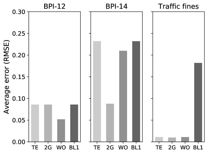
Figure 3: Results accuracy real-world logs (trace-level)

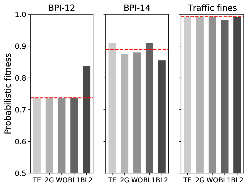
Figure 4: Results accuracy real-world logs (log-level)

Synthetic collection. Figures 6 and 6 visualize the results obtained for the 500 generated process models, over varying noise levels. The figures clearly show that the general trends of the results are preserved across noise levels and apply to both trace and log-level error measurements. In particular, the 2-gram model (2G) here consistently outperforms the other models, achieving a trace-level RMSE ranging from 0.026 (25% noise) to 0.036 (100% noise) and a log-level error between 0.002 and 0.003. At the trace-level, the 2G model is closely followed by the WO model, with an RMSE between 0.030 and 0.042, though Figure 6 clearly reveals a larger difference when considering the log-level. There, the WO model still performs second best, but achieves an error between 0.010 and 0.012, i.e., between 4 and 5 times as large as the error of the 2G model.

When aggregating the accuracy of the behavioral models over all noise levels, we observe that the 2G model achieves an average RMSE of 0.032 and a log-level fitness error of 0.003. By contrast, the WO model model achieves an RMSE of 0.038 (1.2 times as high) and a log-level error of 0.013 (4.3 times as high as the 2G model). The trace equivalence model (TE) performs worst, with an RMSE of 0.042 (1.3 times) and log-level error of 0.015 (4.9 times). Nevertheless, as also depicted, all models considerably outperform both baselines. The uniform probability baseline (BL1) has the worst performance, obtaining an RMSE of 0.078 (2.40 times the error of 2G) and a log-level error of 0.043 (14.3 times as high). BL2, which simply ignored all traces with ordering uncertainty, achieves a log-level error of 0.023 (7.8 times the error of 2G).

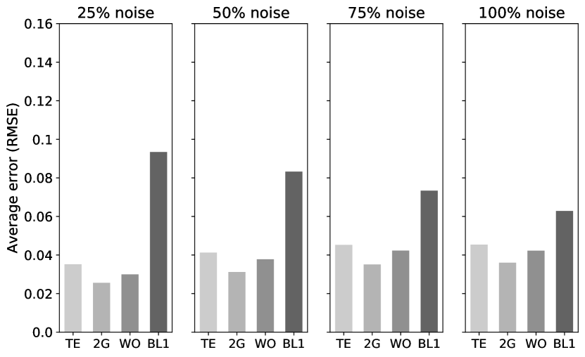
Figure 5: Results accuracy synthetic logs (trace-level)

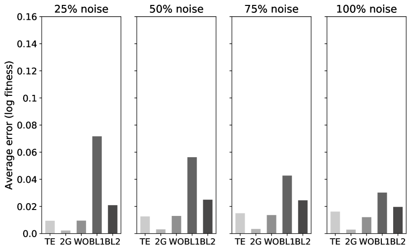
Figure 6: Results accuracy synthetic logs (log-level)

Considering the tracel-level results obtained per event log, we observe some variability among the performance of the behavioral models. Out of the 2000 cases (500 models over 4 noise levels), the 2G model outperforms all other models in the majority of the cases: 1203 times. Surprisingly, the trace equivalence model (TE) performs best for 533 cases, while the weak order model (WO) outperforms the others in 264 cases. There is no event log in the synthetic collection for which the baselines outperform the proposed models.

Impact of order uncertainty. Aside from assessing the accuracy for different noise levels, it is interesting to assess how the degree of uncertainty in an event log affects the conformance checking accuracy. To obtain event logs that cover a broad range of uncertainty degrees, we generated additional event logs for the models in the synthetic data collection using different throughput rates. In particular, for each of the 500 models, we also generated event logs with 0.25, 0.50, and 2.0 times the throughput rate of the event logs used in the experiments described earlier. The idea here is that a higher (lower) throughput rate results in more (fewer) events that have a timestamp within the same minute and, therefore, more (fewer) uncertainty.

We grouped the obtained event logs based on their percentage of traces with order uncertainty, as shown in Table 5. The table reveals the overall expected trend in which the average error increases along with the amount of order uncertainty present in an event log. However, it is interesting to observe that this applies in only a very limited manner to the 2G model, which is both the best performing and most stable model across the various degrees of uncertainty. By contrast, the performance of the TE model quickly decreases with higher uncertainty. This makes sense, given that this model requires traces without any form of uncertainty in order to be able to derive evidence for its probability computation. Although it is more stable than TE, the WO model is outperformed by the 2G model. Finally, the results clearly show that each of the proposed models outperform the baselines. In line with expectations, especially the performance of BL2, which only consider traces without uncertainty, sharply decreases for higher amounts of uncertainty.

Uncertain trace ratio	0.0–0.2	0.2–0.4	0.4–0.6	0.6–0.8	0.8–1.0
Number of event logs	304	1110	877	539	170
Uncertain events (avg.)	7.0%	13.2%	19.5%	25.5%	36.2%
TE	.001	.004	.011	.020	.033
2G	.001	.004	.002	.002	.004
WO	.002	.010	.012	.011	.016
BL1	.006	.038	.046	.044	.049
BL2	.018	.020	.027	.033	.082

Table 5: Log-level error for different levels of uncertainty in synthetic logs

6.3.2 Computational Efficiency

To assess the runtime efficiency of conformance checking under uncertainty and our proposed approximation method, we conducted experiments on a 2017 MacBook Pro (Dual-Core Intel i5) with 3,3GHz and an 8GB Java Virtual Machine.

Real-world collection. The results obtained by applying the approach without and with approximation on the three real-world event logs are shown in Table 6. We here report on the runtimes obtained using the 2G behavioral model, which achieves the overall best performance accuracy. The recorded runtimes highlight that conformance checking in the presence of traces with order uncertainty can take considerable time. Although the Traffic fines log is processed in less than half a second, the BPI-14 log requires almost 40 minutes, whereas the BPI-12 log takes close to 4 hours to process. These lengthy runtimes follow from the combination of various factors: the traffic fines log is has short traces (average length of 3.7 events), a low number of variants (231), and a relatively low amount of uncertainty. This means that the vast majority of its 150,370 traces do not require intensive expensive alignment computation, given that they do not show uncertainty and follow a previously observed trace variant. By contrast, the BPI-12 and BPI-14 event logs have longer traces (20.0 and 7.3 events per trace, respectively), have more variants (4,366 and 31,725) and a higher fraction of uncertainty (38.3% and 93.4% of the traces). The runtime difference between the BPI-12 and BPI-14 logs can, most likely, be attributed to the average length of traces, which is considerably higher for the BPI-12 case (20.0 versus 7.3 average events per trace).

When considering the results including our proposed approximation method, first and foremost, we note that approximation has minimal impact on the conformance checking accuracy. For all real-world logs, the (trace-level) error values obtained when using our approximation method are equal up to 3 decimal places compared to those obtained without using approximation. Our results cover a configuration with $\alpha=0.99$. Yet, experiments with $\alpha=0.95$ yielded near-identical results.

This near-identical accuracy is obtained while potentially achieving considerable improvements in terms of runtime. As shown in Table 6, approximation does not impact the Traffic fines event log. Due to the relatively low order uncertainty in the event log and short trace length, there are no traces for which there are sufficient possible resolutions to trigger the approximation approach. However, we do observe considerable gains for the other two event logs. In particular for the BPI-12 event log, we observed that the approximation method nearly halves the time required to obtain conformance checking results (gaining 47.9% of the runtime). For the BPI-14 log, the runtime improvement is smaller though still notable, with 13.5% of the runtime saved. These results imply that the benefits of the approximation methods are particularly apparent when they are needed most, i.e., for conformance checking settings with otherwise high runtimes. This conclusion is strengthened by also considering the results obtained for the synthetic data collection.

Table 6: Runtime efficiency on the real-world logs.

Measure	BPI-12	BPI-14	Traffic fines
Runtime (no approx. )	237.8m	39.6m	424ms
Runtime (with approx.)	123.8m	34.2m	390ms
Time saved through approx.	114.0m (47.9%)	5.4m (13.5%)	n/a
Traces approximated	1,090 (8.3%)	2,318 (5.6%)	0 (0.0%)
Additional error (RMSE)	0.000	0.000	0.000

Synthetic collection. Table 7 presents the runtime results obtained for the synthetic data collection. We observe that the approximation method achieves considerable time savings, averaging between 58.9% and 45.9% savings per log and a maximum of 85.7% time saved. These gains are achieved while having a limited impact on the conformance checking accuracy of the approach. On average, the additional error incurred based on approximation is between only 0.02% and 0.03%, whereas the maximum additional error is 1.0%.

It is interesting to observe that the approximation method is actually applied to only about 2.0% of the traces with uncertainty, with a maximum of 18.8% in a single log. However, as shown by the much larger gains in runtime, it is clear that the approximation method is applied to traces that contribute the most to the total runtime. This naturally follows from the approximation method’s dependence on the central limit theorem, which enforces that approximation can only be applied to traces with at least 20 possible resolutions. In other words, the approximation method is generally applied to traces with the otherwise largest runtime.

Table 7: Runtime efficiency on the synthetic collection (averages over collection).

	Noise level
Measure	25.0	50.0	75.0	100.0
Time, no approx. (avg.)	12.1s	12.8	13.8s	14.0s
Time, with approx. (avg.)	5.0s	6.0s	6.7s	7.6s
Time saved through approx. (avg.)	58.9%	53.1%	51.2%	45.9%
Time saved through approx. (max.)	85.7%	80.9%	84.6%	80.7%
Traces approximated (avg.)	1.7%	1.9%	2.0%	2.2%
Traces approximated (max.)	17.2%	18.7%	17.9%	18.8%
Approx. error (avg.)	0.03%	0.02%	0.03%	0.02%
Approx. error (max.)	1.00%	0.98%	1.01%	1.00%

6.4 Discussion

The results presented in this section show that the 2G model is generally the best performing one, though there are cases when the WO model and, occasionally the TE model achieve the best accuracy. A factor that plays an important role for the performance of the behavioral models is the amount of information that the model can utilize from the available event log. The higher the abstraction level of a behavioral model, the more information that can be taken into account. The trace equivalence model, the least abstract model, can only derive probabilistic information from traces that do not contain any uncertainty. Even if such traces are available, the model can only provide probabilistic insights if the same trace is repeated for the process. This makes the trace equivalence model inapplicable to logs with a high variety and uncertainty, such as the BPI-14 log, in which over 93% of the traces have uncertainty. This problem can also occur for the 4G and 3G models, which still depend on repeated sequences of events without uncertainty.

Best performing behavioral model. Overall, we conclude that the 2G model performs best. Especially on the widely varying synthetic model collection, the 2G model is shown to achieve the most accurate trace-level and log-level results across all noise levels (Figures 6 and 6) and degrees of uncertainty (Table 5). However, the WO model outperforms the others for the BPI-12 log. This may be attributed to the larger average length of the traces, which may suggest, that in this case, it is more helpful to consider events that indirectly follow each other, rather than only those that directly follow each other. Note that a post-hoc evaluation of the results did not reveal any notable correlation between process model characteristics, such as the presence of loops or non-free choice components, and the accuracy obtained by the different behavioral models.

Impact of approximation. Aside from the selection of a behavioral model, the results from Section 6.3.2 show that the proposed approximation method can be used with little impact on the approach’s accuracy, while gaining considerable benefits in terms of runtime. The preservation of such a high level of result accuracy is due to the method’s grounding in statistical distributions, which requires that at least 20 possible resolutions of a trace are checked before applying approximation.

Applicability of the approach. As defined in our event model presented in Section 3.1, our approach targets cases in which order uncertainty is explicitly captured through the presence of events with identical timestamps. This is a situation that has clearly been shown to be prevalent in practical settings through our analysis of the real-world event logs, as depicted in Table 3. However, we recognize that there are also cases in which order uncertainty exists, but may not be directly visible from the granularity of the available timestamps. For instance, an unreliable sensor may record timestamps in terms of milliseconds, even though the true moment of occurrence can only be guaranteed in terms of seconds. These cases could be detected using approaches such as proposed by Dixit et al. [33]. Following such a detection, a pre-processing step could be employed that abstracts the unreliable timestamps to a granularity at which the uncertainty no longer exists, before employing our proposed approach. In this manner, also such occurrences of order uncertainty can be detected, while maintaining the benefits of our approach in comparison to approaches that impose strict assumptions on the correct order of a trace.

7 Related Work

In this section we discuss the three primary streams to which our work relates: conformance checking, sequence classification, and uncertain data management.

Conformance checking is commonly based on alignments, as discussed in Section 2.1. Due to the computational complexity of alignment-based conformance checking, various angles have been followed to improve its runtime performance. Efficiency improvements have been obtained through the use of search-based methods [34, 35], and planning algorithms [36]. Similar to the approximation method presented in Section 5, several approaches approximate conformance results to gain efficiency, e.g., by employing approximate alignments [37], sampling strategies [38], and applying divide-and-conquer schemes in the computation of conformance results [39, 12, 40]. These approaches can be regarded as complimentary to our approximation method, since our method reduces the number of resolutions for which conformance results need to be obtained, whereas these other approaches improve the efficiency achieved per resolution.

Sequence classification refers to the task of assigning class labels to sequences of events [41], a task with applications, e.g., in genomic analysis, information retrieval, and anomaly detection. A key challenge of sequence classification is the high dimensionality of features, resulting from the sequential nature of events. A broad variety of methods have been developed for this task, which can be generally grouped over three categories [41], i.e., feature-based, distance-based, and model-based methods. In particular the latter methods, which employ techniques such as Hidden Markov Models, may resemble the behavioral models proposed in this work. However, the addressed problem fundamentally differs: Sequence classification assigns labels to sequences, whereas our models aim at determining the actual sequence of events itself.

Data uncertainty is inherent to various application contexts, typically caused by data randomness, incompleteness, or limitations of measuring equipment [42]. This has created a need for algorithms and applications for uncertain data management [43]. These include models for probabilistic and uncertain databases, see [44], along with respective query mechanisms [45]. Moreover, models to capture uncertain event occurrence. This includes models where the event occurrence itself is uncertain [46] as well as those where uncertainty relates only to the time of event occurrence [47], which may be defined by a density function over an interval. Our model, in turn, incorporates the particular aspect of order uncertainty within a trace. The reason being that the probability of an event occurrence at a particular time is of minor importance when assessing conformance of a trace with respect to the execution sequences of a model. Aside from the order uncertainty we consider, uncertainty can also follow from unknown mappings of events to process model activities [48, 49] and from the use of ambiguous process specifications [50].

8 Conclusion

In this paper, we overcame a key assumption of conformance checking that limits its applicability in practical situations: The requirement that the events observed for a case in a process are totally ordered. In particular, we established various behavioral models, each incorporating a different notion of behavioral abstraction. These behavioral models enable the resolution of partial orders by inferring probabilistic information from other process executions. Our evaluation of the approach based on real-world and synthetic data reveal that our approach achieves considerably more accurate results than an existing baseline, reducing the average error by 59%. To cope with the runtime complexity of conformance checking with order uncertainty, we also presented a sample-based approximation method. The conducted experiments demonstrate that this method can lead to considerable runtime reductions, while still obtaining a near-identical conformance checking accuracy.

In our experiments, we focused on conformance on the trace and log level. However, as indicated in Section 3.2, the assignment of probabilities to resolutions is also beneficial for advanced feedback on non-conformance. Measures that quantify conformance may be computed per resolution and then be aggregated based on the assigned probabilities. Similarly, our probabilistic model highlights the overall importance of particular deviations. However, we see open research questions related to the perception of such probabilistic results in conformance checking and intend to explore this aspect in future case studies. We also aim to extend our work with behavioral models that go beyond temporal aspects of event logs. For instance, employing decision mining techniques, multi-perspective models may enable more fine-granular selection of traces for partial order resolution.

Reproducibility: Links to the employed source code and datasets are given in Section 6.

References

- [1] M. Dumas, M. L. Rosa, J. Mendling, H. A. Reijers, Fundamentals of Business Process Management, Second Edition, Springer, 2018.
- [2] W. M. P. V. der Aalst, Process Mining - Data Science in Action, Second Edition, Springer, 2016.
- [3] J. Carmona, B. F. van Dongen, A. Solti, M. Weidlich, Conformance Checking - Relating Processes and Models, Springer, 2018. doi:10.1007/978-3-319-99414-7.
- [4] H. Schonenberg, R. Mans, N. Russell, N. Mulyar, W. Van der Aalst, Process flexibility: A survey of contemporary approaches, in: EOMAS, Springer, 2008, pp. 16–30.
- [5] F. Bagayogo, A. Beaudry, L. Lapointe, Impacts of IT acceptance and resistance behaviors: a novel framework, in: Intl. Conf. Information Systems, 2013.
- [6] R. Lu, S. Sadiq, G. Governatori, Compliance aware business process design, in: Intl. Conf. Business Process Management, Springer, 2007, pp. 120–131.
- [7] F. Caron, J. Vanthienen, B. Baesens, Comprehensive rule-based compliance checking and risk management with process mining, Decision Support Systems 54 (3) (2013) 1357–1369.
- [8] W. Van der Aalst, K. Van Hee, J. M. Van der Werf, A. Kumar, M. Verdonk, Conceptual model for online auditing, Decision Support Systems 50 (3) (2011) 636–647.
- [9] A. Adriansyah, B. van Dongen, W. M. P. Van der Aalst, Conformance checking using cost-based fitness analysis, in: EDOC, IEEE, 2011, pp. 55–64.
- [10] J. C. J. C. Bose, R. S. Mans, W. M. P. Van der Aalst, Wanna improve process mining results?, in: CIDM, IEEE, 2013, pp. 127–134. doi:10.1109/CIDM.2013.6597227.
- [11] R. S. Mans, W. M. P. Van der Aalst, R. J. Vanwersch, A. J. Moleman, Process mining in healthcare: Data challenges when answering frequently posed questions, in: ProHealth, Springer, 2013, pp. 140–153.
- [12] J. Munoz-Gama, J. Carmona, W. v. d. Aalst, Single-entry single-exit decomposed conformance checking, Inf. Syst. 46 (2014) 102–122.
- [13] S. Suriadi, R. Andrews, A. H. ter Hofstede, M. T. Wynn, Event log imperfection patterns for process mining: Towards a systematic approach to cleaning event logs, Inf. Syst. 64 (2017) 132–150.
- [14] S. Suriadi, C. Ouyang, W. M. van der Aalst, A. H. ter Hofstede, Event interval analysis: Why do processes take time?, Decision Support Systems 79 (2015) 77–98.
- [15] C. Batini, M. Scannapieco, Data Quality: Concepts, Methodologies and Techniques, Data-Centric Systems and Applications, Springer, 2006. doi:10.1007/3-540-33173-5.
- [16] E. Koskinen, J. Jannotti, Borderpatrol: isolating events for black-box tracing, in: J. S. Sventek, S. Hand (Eds.), Proc. 2008 EuroSys Conference, ACM, 2008, pp. 191–203. doi:10.1145/1352592.1352613.
- [17] C. Mutschler, M. Philippsen, Reliable speculative processing of out-of-order event streams in generic publish/subscribe middlewares, in: Proc. 7th Intl. Conf. Distr. Event-based Syst., 2013, pp. 147–158.
- [18] X. Lu, R. S. Mans, D. Fahland, W. M. P. Van der Aalst, Conformance checking in healthcare based on partially ordered event data, in: ETFA, IEEE, 2014, pp. 1–8.
- [19] T. T. L. Tran, C. A. Sutton, R. Cocci, Y. Nie, Y. Diao, P. J. Shenoy, Probabilistic inference over RFID streams in mobile environments, in: Proc. 25th Intl. Conf. Data Engineering ICDE, 2009, pp. 1096–1107.
- [20] N. Busany, H. van der Aa, A. Senderovich, A. Gal, M. Weidlich, Interval-based queries over lossy iot event streams, ACM Transactions on Data Science (in press).
- [21] A. Senderovich, A. Rogge-Solti, A. Gal, J. Mendling, A. Mandelbaum, The ROAD from sensor data to process instances via interaction mining, in: CAISE, 2016, pp. 257–273.
- [22] S. Chen, J. L. Moore, D. Turnbull, T. Joachims, Playlist prediction via metric embedding, in: SIGKDD, ACM, 2012, pp. 714–722.
- [23] M. Mohri, F. Pereira, M. Riley, Weighted finite-state transducers in speech recognition, Computer Speech & Language 16 (1) (2002) 69–88.
- [24] M. Rosenblatt, A central limit theorem and a strong mixing condition, Proceedings of the National Academy of Sciences of the United States of America 42 (1) (1956) 43.
- [25] A. Agresti, B. A. Coull, Approximate is better than “exact” for interval estimation of binomial proportions, The American Statistician 52 (2) (1998) 119–126.
- [26] S. L. Lohr, Sampling: Design and Analysis: Design and Analysis, Chapman and Hall/CRC, 2019.
- [27] S. J. Leemans, D. Fahland, W. M. P. Van der Aalst, Discovering block-structured process models from event logs-a constructive approach, in: Petri nets, Springer, 2013, pp. 311–329.
- [28] Van Dongen, B.F. (Boudewijn), Bpi challenge 2012 (2012). doi:10.4121/UUID:3926DB30-F712-4394-AEBC-75976070E91F.
- [29] B. Van Dongen, BPI Challenge 2014 (2014). doi:10.4121/uuid:c3e5d162-0cfd-4bb0-bd82-af5268819c35.
- [30] M. M. De Leoni, F. F. Mannhardt, Road traffic fine management process (2015). doi:10.4121/UUID:270FD440-1057-4FB9-89A9-B699B47990F5.
- [31] T. Jouck, B. Depaire, Generating artificial data for empirical analysis of control-flow discovery algorithms: A process tree and log generator, BISE (2018) 1–18.
- [32] A. Rogge-Solti, M. Weske, Prediction of remaining service execution time using stochastic petri nets with arbitrary firing delays, in: ICSOC, Springer, 2013, pp. 389–403.
- [33] P. M. Dixit, S. Suriadi, R. Andrews, M. T. Wynn, A. H. ter Hofstede, J. C. Buijs, W. M. van der Aalst, Detection and interactive repair of event ordering imperfection in process logs, in: International Conference on Advanced Information Systems Engineering, Springer, 2018, pp. 274–290.
- [34] D. Reißner, R. Conforti, M. Dumas, M. L. Rosa, A. Armas-Cervantes, Scalable conformance checking of business processes, in: OTM to Meaningful Int. Syst., 2017, pp. 607–627. doi:10.1007/978-3-319-69462-7\_38.
- [35] B. F. van Dongen, Efficiently computing alignments - using the extended marking equation, in: Business Process Management, 2018, pp. 197–214. doi:10.1007/978-3-319-98648-7\_12.
- [36] M. de Leoni, A. Marrella, How planning techniques can help process mining: The conformance-checking case, in: Italian Symp. on Advanced Database Syst., 2017, p. 283.
- [37] F. Taymouri, J. Carmona, A recursive paradigm for aligning observed behavior of large structured process models, in: Business Process Management, Springer, 2016, pp. 197–214. doi:10.1007/978-3-319-45348-4\_12.
- [38] M. Bauer, H. van der Aa, M. Weidlich, Estimating process conformance by trace sampling and result approximation, in: Business Process Management, Springer, 2019, pp. 179–197.
- [39] W. M. P. V. der Aalst, H. M. W. Verbeek, Process discovery and conformance checking using passages, Fundam. Inform. 131 (1) (2014) 103–138. doi:10.3233/FI-2014-1006.
- [40] S. J. J. Leemans, D. Fahland, W. M. P. V. der Aalst, Scalable process discovery and conformance checking, Software and System Modeling 17 (2) (2018) 599–631. doi:10.1007/s10270-016-0545-x.
- [41] Z. Xing, J. Pei, E. Keogh, A brief survey on sequence classification, SIGKDD Explor 12 (1) (2010) 40–48.
- [42] J. Pei, B. Jiang, X. Lin, Y. Yuan, Probabilistic skylines on uncertain data, in: Proc. 33rd Intl. Conf. Very large data bases, 2007, pp. 15–26.
- [43] C. C. Aggarwal, P. S. Yu, A survey of uncertain data algorithms and applications, IEEE Trans. Knowl. Data Eng. 21 (5) (2009) 609–623.
- [44] L. Peng, Y. Diao, Supporting data uncertainty in array databases, in: SIGMOD Intl. Conf. Mgt. of Data, ACM, 2015, pp. 545–560.
- [45] R. Murthy, R. Ikeda, J. Widom, Making aggregation work in uncertain and probabilistic databases, IEEE Trans. Knowl. Data Eng. 23 (8) (2011) 1261–1273.
- [46] C. Ré, J. Letchner, M. Balazinska, D. Suciu, Event queries on correlated probabilistic streams, in: J. T. Wang (Ed.), Proc. SIGMOD Intl. Conf. Mgt. of Data, SIGMOD, ACM, 2008, pp. 715–728. doi:10.1145/1376616.1376688.
- [47] H. Zhang, Y. Diao, N. Immerman, Recognizing patterns in streams with imprecise timestamps, Inf. Syst. 38 (8) (2013) 1187–1211. doi:10.1016/j.is.2012.01.002.
- [48] H. Van der Aa, H. Leopold, H. A. Reijers, Efficient process conformance checking on the basis of uncertain event-to-activity mappings, TKDE 32 (5) (2020) 927–940.
- [49] T. Baier, J. Mendling, M. Weske, Bridging abstraction layers in process mining, Inf. Syst. 46 (2014) 123–139.
- [50] H. Van der Aa, H. Leopold, H. A. Reijers, Checking process compliance against natural language specifications using behavioral spaces, Inf. Syst. 78 (2018) 83–95.