Analysis of Neural Clusters due to
Deep Brain Stimulation Pulses

Abstract

Deep brain stimulation (DBS) is an established method for treating pathological conditions such as Parkinson’s disease, dystonia, Tourette syndrome, and essential tremor. While the precise mechanisms which underly the effectiveness of DBS are not fully understood, theoretical studies of populations of neural oscillators stimulated by periodic pulses suggest that this may be related to clustering, in which subpopulations of the neurons are synchronized, but the subpopulations are desynchronized with respect to each other. The details of the clustering behavior depend on the frequency and amplitude of the stimulation in a complicated way. In the present study, we investigate how the number of clusters, their stability properties, and their basins of attraction can be understood in terms of one-dimensional maps defined on the circle. Moreover, we generalize this analysis to stimuli that consist of pulses with alternating properties, which provide additional degrees of freedom in the design of DBS stimuli. Our results illustrate how the complicated properties of clustering behavior for periodically forced neural oscillator populations can be understood in terms of a much simpler dynamical system.

1 Introduction

A primary motivation for this study is Parkinson’s disease, which can cause an involuntary shaking that typically affects the distal portion of the upper limbs, and difficulty initiating motion. For patients with advanced Parkinson’s disease who do not respond to drug therapy, electrical deep brain stimulation (DBS), an FDA-approved therapeutic procedure, may offer relief bena91 . Here, a neurosurgeon guides a small electrode into the sub-thalamic nucleus or globus pallidus interna (GPi); the electrode is connected to a pacemaker implanted in the chest which sends periodic electrical pulses directly into the brain tissue. The efficacy of DBS for the treatment of Parkinson’s disease has been found to depend on the frequency of stimulation, with high-frequency stimulation (70 to 1000 Hz and beyond) being therapeutically effective bena91 ; rizz01 ; moro02 . The generally accepted therapeutic range is 130-180 Hz volk02 ; kunc04 . Experimental evidence has suggested that motor symptoms of Parkinson’s disease are associated with pathological synchronization of neurons in the basal ganglia, and that DBS desynchronizes the neural activity uhlh06 ; chen07 ; hamm07 ; levy00 ; schn05 . DBS has also shown promising results in treating other neurological conditions, for which the stimulation electrode is implanted in the GPi (for dystonia) or the thalamus (for Tourette syndrome and essential tremor) savi12 ; bena02 .

While the precise mechanisms which underly the effectiveness of DBS are not fully understood, theoretical studies have shown that DBS-like stimulation consisting of a periodic pulses applied to neural oscillator populations can lead to chaotic desynchronization wils11 or clustering behavior wils15cluster , in which subpopulations of the neurons are synchronized, but the subpopulations are desynchronized with respect to each other. Clustering has also been found in theoretical studies of coordinated reset, in which multiple electrodes deliver inputs which are separated by a time delay luck13 ; lysy11 ; lysy13 ; tass03a . These studies, along with clinical successes with coordinated reset adam14 , point to clustering as an attractive objective for designing stimulation properties; this has motivated the design of single control inputs which promote clustering matc18 ; mong19_physicad ; wils20 , in contrast to methods which seek to fully desynchronize the neural activity tass03 ; nabi13 ; wils14a ; mong20 . Notably, clustering has at least two important differences from chaotic desynchronization: clustered states often exist over a much larger parameter range than chaotic desynchronization, a possible explanation why effective DBS parameters are easier to find than chaotic desynchronization would suggest; and clustered states may induce plasticity changes more effectively than chaotic desynchronization, which may explain why benefits are more persistent for some kinds of stimulation mechanisms than others (cf. adam14 ; mong19_physicad ). In this paper, we will focus on clustering which arises from a single stimulation electrode, unlike coordinated reset which uses multiple electrodes.

Despite substantial data backing the general efficacy of DBS, it can have side effects including disorientation, memory deficits, spatial delayed recall, response inhibition, episodes of mania, hallucinations, or mood swings, as well as impairment of social functions such as the ability to recognize the emotional tone of a face cyro16 ; buhm17 . Our study develops tools which can help to identify different stimuli that result in the same clustering behavior; our hope is that the identification of these alternatives will allow neurologists to consider different stimuli in order to find those which are effective at treating neurological disorders while minimizing the severity of side effects.

In this paper, we investigate how the details of clustering due to periodic pulses of the type used in DBS can be understood in terms of one-dimensional maps defined on the circle. As a first step, Section 2 describes phase reduction, a powerful classical technique for the analysis of oscillators in which a single variable describes the phase of the oscillation with respect to some reference state. Section 3 shows results from simulations of populations of neural ocsillators stimulated by periodic pulses of the type used for DBS; this illustrates the different types of clustering which can occur, and motivates the theoretical analysis. Section 4 derives and investigates the one-dimensional maps which can be used to understand the types of clusters which occur, their stability properties, and their basins of attraction. Section 5 then demonstrates how this analysis in terms of maps can be generalized to consider stimuli that consist of pulses with alternating properties, which provide additional degrees of freedom for DBS stimulus design. Section 6 summarizes the results. The models for the neurons considered in this paper are given in the Appendix.

2 Phase Reduction

A common way to describe the dynamics of neurons is to use conductance-based models such as the Hodgkin-Huxley equations hodg52d . Such models are typically high-dimensional and contain a large number of parameters, which can make them unwieldy for simulations of large neural populations. A powerful technique for the analysis of oscillatory neurons, whose dynamics are described by a stable periodic orbit, is the rigorous reduction of conductance-based models to phase models, with a single variable $\theta$ describing the phase of the oscillation with respect to some reference state winf01 ; kura84 ; mong19 .

Suppose that our conductance-based model is described by the $n$-dimensional dynamical system

$$\frac{d{\bf x}}{dt}={\bf F}({\bf x}),\qquad{\bf x}\in\mathbb{R}^{n}\quad(n\geq 2),$$ (1)

with a stable periodic orbit $\gamma(t)$ with period $T$. For each point ${\bf x}^{\ast}$ in the basin of attraction of $\gamma(t)$ there exists a corresponding phase $\theta$(${\bf x}^{\ast}$) such that guck75 ; winf01

$$\lim\limits_{t\to\infty}\left|{\bf x}(t)-\gamma\left(t+\frac{T}{2\pi}\theta({\bf x}^{\ast})\right)\right|=0,$$ (2)

where, under the given vector field, ${\bf x}(t)$ is the trajectory of the initial point ${\bf x}^{\ast}$. The asymptotic phase of ${\bf x}$, $\theta({\bf x})$, ranges in value from $[0,2\pi)$. In this paper, $\theta=0$ will represent the phase at which the neuron fires an action potential. Isochrons are level sets of $\theta({\bf x})$, and we define isochrons such that the phase of a trajectory evolves linearly in time both on and off of the periodic orbit winf67 ; winf01 . As a result, for the entire basin of attraction of the periodic orbit,

$$\frac{d\theta}{dt}=\frac{2\pi}{T}\equiv\omega.$$ (3)

If we now consider the dynamical system

$$\frac{d{\bf x}}{dt}={\bf F}({\bf x})+{\bf U}(t),\qquad{\bf x}\in\mathbb{R}^{n},$$ (4)

where ${\bf U}(t)\in\mathbb{R}^{n}$ is an infinitesimal control input, phase reduction gives the one-dimensional system kura84 ; brow04 ; mong19

$$\frac{d\theta}{dt}=\omega+{\bf U}(t)^{T}{\bf Z}(\theta).$$ (5)

In this equation, ${\bf Z}(\theta)$ is the gradient of $\theta$ evaluated on the periodic orbit, and is known as the phase response curve (PRC) winf01 ; erme10 ; neto12 ; it represents the change in phase that the control input will cause when applied at a given phase. In this paper, we consider electrical current inputs which only act in the voltage direction defined by the unit vector $\hat{V}$, i.e., ${\bf U}(t)=u(t)\hat{V}$, with the corresponding phase reduction

$$\frac{d\theta_{i}}{dt}=\omega+Z(\theta_{i})u(t).$$ (6)

Here, $\theta_{i}$ represents the phase of the $i^{\rm th}$ neuron, $\omega$ is the natural frequency of the neuron in radians per second, $Z(\theta)=\frac{\partial\theta}{\partial V}$ is the component of the PRC in the voltage direction, and $u(t)$ is the input. For the populations of neurons considered in this paper, we assume that the neurons are identical and they all receive the same input, and we will consider uncoupled neurons without noise; these assumptions allow a more detailed analysis to be performed.

In the next section, we show simulation results for populations of neurons described by such phase models with periodic pulses of the type used for DBS.

3 Simulation Results for Identical Periodic DBS Pulses

In this section, we show simulation results for populations of neurons stimulated by periodic pulses of the type used for DBS; these results will inspire the analysis in Section 4. To illustrate a range of clustering behaviors, we show simulations for prototypical systems which represent two common types of neurons rinz98 : as a Type I neuron model, we consider the model for thalamic neurons from rubi04 , and as a Type II model we consider the Hodgkin-Huxley equations hodg52d . These models are not meant to correspond to the neurons directly relevant to Parkinson’s disease in human patients; rather, they are used to illustrate typical clustering behaviors for populations of neural oscillators under DBS-like stimuli. The full equations and parameters for these models are given in the Appendix. For our simulations, we use the corresponding phase models. For reference, for these parameters the thalamic neurons have $\omega=0.748$ rad/s, and the Hodgkin-Huxley neurons have $\omega=0.429$ rad/s. The PRC functions for these neurons are shown in Figure 1(a) and (b), respectively. Each PRC was calculated numerically using XPP erme02 , and is approximated by a Fourier series.

Figure 1: Panels (a) and (b) show the phase response curves $Z(\theta)$ of the thalamic (Type I) and Hodgkin-Huxley (Type II) neurons considered in this paper, respectively.

Figure 2: Periodic sequence of identical pulses.

The input $u(t)$ that we consider, shown in Figure 2 and inspired by DBS stimuli mont10 , is a periodic sequence of identical charge-balanced pulses parameterized by amplitude $u_{max}$, period $\tau$ (with corresponding frequency $1/\tau$), pulse width $p$, and multiplier $\lambda$ (the ratio of time that the pulse is negative to the time that the pulse is positive). Mathematically, $u(t)$ is given by:

$$u(t)=\left\{\begin{array}[]{ll}u_{max}&\bmod(t,\tau)\leq p\\ u_{min}\equiv-\frac{u_{max}}{\lambda}&p<\bmod(t,\tau)\leq(\lambda+1)p\\ 0&$otherwise$.\end{array}\right.$$ (7)

Unless otherwise stated, we will use $u_{max}$ corresponding to a current density of $20\mu A/cm^{2}$, $p=0.5$ ms, and $\lambda=3$ in our simulations. We consider different frequencies of stimulation between 70-300 Hz, which includes the typical therapeutic range of 130-180 Hz for DBS treatment of Parkinson’s disease.

We simulated 500 Hodgkin-Huxley neurons with initial phases evenly spaced between $0$ and $2\pi$, corresponding to an initial uniform phase distribution. The stimulation frequency was varied from 70 Hz to 300 Hz in increments of 5 Hz. Figure 3 shows the final phases after 40 periods of stimulation, after transients have decayed away. The colors indicate the initial phases of the neurons. Not all colors are visible for most stimulation frequencies because the final phases of entire subpopulations of neurons are nearly identical, and only one representative initial phase can be seen. All of the neurons which have nearly the same final phase are part of the same cluster.

Figure 4 shows the times series of the phases of a population of Hodgkin-Huxley neurons for selected frequencies, and helps us to interpret the results shown in Figure 3. For example, Figure 4(a) shows that for a $100$ Hz stimulus the neurons separate into three clusters, as is also the case for $250$ Hz as shown in Figure 4(e). (Notice that Figure 3 shows three possible final phases for each of these frequencies, corresponding to these three clusters.) Figure 4(b) shows that for a $150$ Hz stimulus they separate into two clusters. For a $180$ Hz stimulus, there is no clustering; see Figure 4(c). By carefully looking at Figure 4(d), one sees that for a $185$ Hz stimulus there are five clusters, and from Figure 4(f) that for a $295$ Hz stimulus there are seven clusters, as expected from final states shown at these frequencies in Figure 3. Such clustering behavior and non-clustering (chaotic) behavior has been seen in other studies, such as wils11 and wils15cluster .

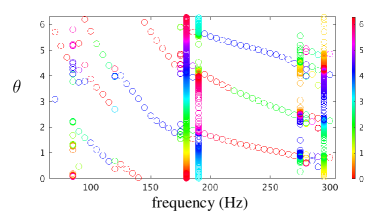
Figure 3: The final phases $\theta$ of Hodgkin-Huxley neurons drawn from an initial uniform distribution as a function of stimulation frequency, after 40 periods of stimulation. Colors correspond to the neurons’ initial phases.

Figure 4: Time series showing the phases of Hodgkin-Huxley neurons drawn from an initial uniform distribution for frequencies (a) 100 Hz, (b) 150 Hz, (c) 180 Hz, (d) 185 Hz, (e) 250 Hz, and (f) 290 Hz. The titles of these panels indicate the number of clusters found after transients have decayed away. For (c), clusters do not form. For this and subsequent time series figures, $t$ is measured in ms, and the colors indicate the initial phases of the neurons, with colorbar as in Figure 3.

Inspired by neural synchrony in Parkison’s patients, we also considered an initial partially synchronized neural population, with phases distributed according to a von Mises distribution best79 centered at $\theta=0$:

$$\rho_{0}(\theta)=\frac{e^{\kappa\cos\theta}}{2\pi I_{0}(\kappa)},$$ (8)

where $I_{0}(\kappa)$ is the modified Bessel function of order 0. This distribution is similar to a Gaussian distribution, but on a circle. We simulated 500 Hodgkin-Huxley neurons with initial phases distributed according to the von Mises distribution with $\kappa=50$. As for Figure 3, the stimulation frequency was varied from 70 Hz to 300 Hz in increments of 5 Hz. Figure 5 shows the final phases after 40 periods of stimulation, after transients have decayed away. We see that the final phases of the neurons from the initial von Mises distribution lie on a subset of the final phases of the neurons from the intial uniform distribution. For example, when the stimulation frequency is 100 Hz, the neurons from the initial von Mises distribution are concentrated in two of the three clusters which exist for the initial uniform distribution.

Figure 5: As a function of stimulation frequency, the final phases $\theta$ of Hodgkin-Huxley neurons drawn from an initial von Mises distribution after 40 periods of stimulation are shown as black $*$’s, overlaid on the final phases of Hodgkin-Huxley neurons drawn from an initial uniform distribution (as was shown in Figure 3).

We also designed an algorithm to detect the size of clusters in a population. The algorithm groups the phases of neurons in a population at each timestep into clusters by sorting the phases in ascending order and checking if the $i^{\rm th}$ phase is within $\epsilon$ of the $(i+1)$-th phase for an appropriate small value of $\epsilon$. If so, the size of the current cluster is increased by one. If not, the algorithm creates a new cluster. The process is repeated until all neurons have been grouped into clusters. Figure 6 shows the number of neurons in the different clusters over a range of frequencies for the intial uniform distribution (for which three clusters are populated) and von Mises distribution (for which only two clusters are populated). As we will see in Section 4, this figure can be explained in terms of the basins of attraction of fixed points of iterates of a one-dimensional map defined on the circle. The initial phase of a given neuron will determine which cluster it ends up in.

Figure 6: The number of Hodgkin-Huxley neurons in different clusters for a population size of 500, with initial (a) uniform and (b) von Mises distributions.

We also considered populations of thalamic (Type I) neurons with the same stimuli (7) with $u_{max}$ corresponding to a current density of $20$ $\mu A/cm^{2}$, $p=0.5$ ms, and $\lambda=3$. We simulated 500 thalamic neurons with initial phases evenly spaced between $0$ and $2\pi$, corresponding to a uniform distribution. The stimulation frequency was varied from 70 Hz to 300 Hz in increments of 5 Hz. Figure 7 shows the final phases after 40 periods of stimulation, after transients have decayed. Figure 8 shows the time series of the phases of a population of such neurons for selected frequencies. Here we again see clustering for some frequencies (such as $250$ Hz), and non-clustering behavior for other frequencies (such as $200$ Hz).

Figure 7: The final phases $\theta$ of thalamic neurons drawn from an initial uniform distribution as a function of stimulation frequency, after 40 periods of stimulation. Colors correspond to the neurons’ initial phases.

Figure 8: Time series showing the phases of thalamic neurons drawn from an initial uniform distribution for frequencies (a) 200 Hz, and (b) 250 Hz. For (a), clusters do not form; for (b), there are two clusters after transients decay away.

In the next section, we derive and investigate one-dimensional maps which can be used to understand the types of clusters which occur in these simulations, along with their stability properties and their basins of attraction.

4 Analysis of Clusters due to Identical Pulses

In this section, we show how the clustering behavior found in the simulations from Section 3 can be understood in terms of appropriate compositions of one-dimensional maps on the circle.

We consider a system of neural oscillators subjected to a $\tau$-periodic sequence of pulses as shown in Figure 2, and described by the dynamics wils15cluster

$$\dot{\theta}_{i}=\omega+f(\theta_{i})\delta({\rm mod}(t,\tau)),\qquad i=1,\cdots,N.$$ (9)

Here the response function $f(\theta)$ describes the change in phase due to a single pulse (including the positive current for time $p$, and the negative current for time $\lambda p$). If the pulse was a delta function with unit area, $f(\theta)$ would be equal to the infinitesimal PRC $Z(\theta)$; for more general pulses, it can be calculated using a direct method in which a pulse is applied at a known phase, and the change in phase is deduced from the change in timing of the next action potential neto12 . We will think of the change in phase due to the pulse as occurring instantaneously, even though the pulse will typically have a finite duration; this will be a good approximation for pulses of short duration. Figure 9 shows $f(\theta)$ for the Hodgkin-Huxley neurons considered in this paper for pulses as shown in Figure 2 with $u_{max}$ corresponding to a current density of $20\mu A/cm^{2}$, $p=0.5$ ms, and $\lambda=3$.

Figure 9: Response function $f(\theta)$ which characterizes the phase response of Hodgkin-Huxley neurons to the stimulus, for $u_{max}$ corresponding to a current density of $20\mu A/cm^{2}$, $p=0.5$ ms, and $\lambda=3$.

To understand the clustering behavior, it will be useful to consider the map which takes the phase of a neuron to the phase exactly one forcing cycle later, cf. wils15cluster . To find this map, suppose that we start with $\theta(0^{+})=0$, immediately after the start of a pulse, where we assume that we have already accounted for the effect of the pulse according to the function $f(\theta)$. The next pulse comes at time $\tau$. Up until time $\tau$, the phase evolves according to $\dot{\theta}=\omega$; therefore,

$$\theta(\tau^{-})=\theta_{0}+\omega\tau.$$ (10)

Treating the change in phase due to the next pulse as occurring instantaneously, we have

$$\theta(\tau^{+})=\theta_{0}+\omega\tau+f(\theta_{0}+\omega\tau).$$ (11)

The system then evolves for a time $\tau$ without stimulus, giving

$$\theta(2\tau^{-})=\theta_{0}+2\omega\tau+f(\theta_{0}+\omega\tau);$$ (12)

the next pulse at time $2\tau$ gives

$$\theta(2\tau^{+})=\theta_{0}+2\omega\tau+f(\theta_{0}+\omega\tau)+f(\theta+2\omega\tau+f(\theta_{0}+\omega\tau)),$$ (13)

and so on. It is useful to let wils15cluster

$$g(s)=s+\omega\tau+f(s+\omega\tau),$$ (14)

which gives

$$\theta(n\tau^{+})=g^{(n)}(\theta_{0}),$$ (15)

where $g^{(n)}$ denotes the composition of $g$ with itself $n$ times, and $\theta_{0}$ is the initial state of the neuron.

We look for fixed points of $g^{(n)}$, that is, solutions to $\theta^{*}=g^{(n)}(\theta^{*})$; for such solutions, the phase has the same value after $n$ pulses as where it started. We are particularly interested in fixed points of $g^{(n)}$ which are not fixed points of $g^{(m)}$ for any positive integer $m$ satisfying $m<n$; then there will be $n$ fixed points of $g^{(n)}$ that correspond to points on a period-$n$ orbit of $g$. If

$$\left|\left.\frac{d}{d\theta}\right|_{\theta=\theta^{*}}(g^{(n)}(\theta))\right|<1,$$ (16)

then the fixed point $\theta^{*}$ of $g^{(n)}$ is stable, as is the corresponding period-$n$ orbit of $g$. Neurons which start with initial phases within the basin of attraction of a given fixed point of $g^{(n)}$ will asymptotically approach that fixed point under iterations of $g^{(n)}$. The $n$ different fixed points will each have a basin of attraction, so a uniform intial distribution of neurons will form $n$ clusters, one for each of these fixed points of $g^{(n)}$, cf. wils15cluster .

We now illustrate how these maps can be used to understand the specific clustering behavior shown in Section 3. As a first example, suppose that a population of Hodgkin-Huxley neurons is stimulated with frequency 150 Hz, corresponding to $\tau=6.67$ ms. Figure 10 shows $g(\theta)$ and $g^{(2)}(\theta)$. Fixed points of these maps correspond to intersections with the diagonal. We see that there are two stable fixed points for $g^{(2)}(\theta)$, at $\theta=2.86$ and $\theta=5.86$ (these fixed points are stable because the slope at the intersection is between $-1$ and $+1$). There are also two unstable fixed points for $g^{(2)}$ at $\theta=1.305$ and $\theta=4.685$, where the slope at the intersection is greater than 1. There are no fixed points for $g(\theta)$, but a cobweb analysis verifies that there is a period-2 orbit

$$\theta=2.86\rightarrow 5.86\rightarrow 2.86\rightarrow\cdots.$$

These fixed points of $g^{(2)}$ correspond a stable 2-cluster state for a population of oscillators, as shown in Figure 4(b). We note that we can deduce the basin of attraction for the different stable fixed points of $g^{(2)}$; for example, the basin of attraction for the stable fixed point at $\theta=2.86$ is the range $1.305<\theta_{0}<4.685$, that is, between the two unstable fixed points.

Figure 10: Maps $g(\theta)$ and $g^{(2)}(\theta)$ for Hodgkin-Huxley neuron with stimulation frequency $150$ Hz. Intersections with the diagonal dashed line indicate fixed points of the respective map. The dotted lines show $\theta$ values for the stable fixed points of the $g^{(2)}$ map.

As another example, suppose that a population of Hodgkin-Huxley neurons is stimulated with frequency 100 Hz, corresponding to $\tau=10$ ms. Figure 11 shows $g(\theta)$ and $g^{(3)}(\theta)$. We see that there are three stable fixed points for $g^{(3)}(\theta)$, at $\theta=1.43$, $\theta=3.37$, and $\theta=5.86$ (these fixed points are stable because the slope at the intersection has slope between $-1$ and $+1$). There are no fixed points for $g(\theta)$, but a cobweb analysis verifies that there is a period-3 orbit

$$\theta=1.43\rightarrow 5.86\rightarrow 3.37\rightarrow 1.43\rightarrow\cdots.$$

These fixed points of $g^{(3)}$ correspond a stable 3-cluster state for a population of oscillators, as shown in Figure 4(a).

Figure 11: Maps $g(\theta)$ and $g^{(3)}(\theta)$ for Hodgkin-Huxley neuron with stimulation frequency $100$ Hz.

We see that this map can also capture $n$-clusters for larger values of $n$. For example, for frequency 185 Hz, the $g$ and $g^{(5)}$ maps shown in Figure 12 confirm that there is a stable period-5 orbit

$$\theta=1.62\rightarrow 3.38\rightarrow 5.85\rightarrow 2.05\rightarrow 5.51\rightarrow 1.62\rightarrow\cdots,$$

corresponding to the stable 5-cluster state shown in Figure 4(d).

Figure 12: Maps $g(\theta)$ and $g^{(5)}(\theta)$ for Hodgkin-Huxley neuron with stimulation frequency $185$ Hz.

Finally, if we apply these identical stimuli at $300$ Hz, we obtain a total of four stable fixed points for $g^{(4)}$, corresponding to a stable period-4 orbit for $g(\theta)$

$$\theta=0.82\rightarrow 2.61\rightarrow 3.32\rightarrow 5.69\rightarrow 0.82\rightarrow\cdots\$$

which is equivalent to two stable period-2 orbits for $g^{(2)}$

$$\theta=0.82\rightarrow 3.32\rightarrow 0.82\rightarrow\cdots,$$

$$\theta=2.61\rightarrow 5.69\rightarrow 2.61\rightarrow\cdots,$$

and four stable fixed points for $g^{(4)}$

$$\theta=0.82,\qquad\theta=2.61,\qquad\theta=3.32,\qquad\theta=5.69;$$

see Figure 13. We show in the next section that it is possible to obtain similar dynamics with stimuli consisting of pulses with alternating properties.

Figure 13: For the Hodgkin-Huxley neurons with stimulation frequency $300$ Hz, there is a stable period-4 orbit for $g$, which corresponds to two stable period-2 orbits for $g^{(2)}$, which in turn correspond to four stable fixed points for $g^{(4)}$.

We can understand the cluster sizes shown in Figure 6(a) by looking at the basins of attraction of the different stable fixed points, as indicated in Figure 14 for $200$ Hz and $260$ Hz stimuli. The basin boundaries are at the phases of the appropriate unstable fixed points. When the initial phase distribution is uniform, the number of neurons which end up in each cluster is proportional to the size of the corresponding basin of attraction. For example, if there are 500 uniformly distributed neurons, this predicts that there will be 144, 173, and 183 neurons in Clusters I, II, and III, respectively, for a $200$ Hz stimluus, and 209, 133, and 159 neurons in Clusters I, II, and III, respectively, for a $260$ Hz stimulus. This is consistent with the results shown in Figure 6(a). The number of neurons in each cluster for Figure 6(b) would be determined by the number of neurons which are initially in the respective basin of attraction, as determined by the initial phase distribution; here, there were no neurons with initial phases that end up in Cluster III.

Figure 14: Basins of attraction for the different clusters for (a) $200$ Hz and (b) $260$ Hz stimuli.

The same analysis techniques can also be used to understand the dynamics of thalamic neurons subjected to periodic pulses. Figure 15(a) shows the response function $f(\theta)$ for thalamic neurons with the stimulus given by (7) with $u_{max}$ corresponding to a current density of $20\mu A/cm^{2}$, $p=0.5$ ms, and $\lambda=3$; Figure 15(b) shows that there is a stable 2-cluster state for a stimulation frequency of $250$ Hz, as expected from Figure 7.

Figure 15: (a) Response function $f(\theta)$ which characterizes the phase response of thalamic neurons to a pulse with $u_{max}$ corresponding to a current of $20\mu A/cm^{2}$, $p=0.5$ ms, and $\lambda=3$. (b) Map $g^{(2)}(\theta)$ for the thalamic neuron with stimulation frequency $250$ Hz, showing two stable fixed points which correspond to a 2-cluster state.

5 Analysis of Clusters due to Pulses with Alternating Properties

In this section, we consider more general stimuli, specifically pulses with alternating properties, as shown in Figure 16. Here, the pulses from before, that is with $u_{max}$ corresponding to a current density of $20\mu A/cm^{2}$, $p=0.5$ ms, and $\lambda=3$, will be assumed to occur at times $0,\tau,2\tau,\cdots$. But now additional pulses with $u_{2max}$ corresponding to a current density of $10\mu A/cm^{2}$, $\lambda=3$, $u_{2min}=-u_{2max}/\lambda$ and $p=0.5$ ms, will be assumed to occur at times $\tau_{2}$, $\tau+\tau_{2}$, $2\tau+\tau_{2},\cdots$. Figure 17 shows that the clustering behavior for such alternating pulses with $\tau_{2}=\tau/2$ strongly resembles the clustering behavior found at twice the frequency for identical pulses, as shown in Figure 3, although there are differences. The analysis in this section shows how the methods from Section 4 can be adapted to understand clustering behavior for such alternating pulses.

Figure 16: Sequence of alternating pulses.

Figure 17: The final phases $\theta$ of Hodgkin-Huxley neurons drawn from an initial uniform distribution as a function of stimulation frequency, after 80 periods of pulses with alternating properties (to allow transients to decay), as described in the text. Colors correspond to the neurons’ initial phases.

Figure 18: Response function $f_{2}(\theta)$ which characterizes the phase response of a Hodgkin-Huxley neuron to a pulse with $u_{2max}$ corresponding to a current density of $10\mu A/cm^{2}$, $u_{2min}=-u_{2max}/3$, and $p=0.5$ ms.

It will again be useful to consider the map which takes the phase of a neuron to its phase at a time $\tau$ later. To formulate this map, we need the response curves for each type of pulse: the response curve $f(\theta)$ for the pulse with $u_{max}$ corresponding to $20\mu A/cm^{2}$ was already shown in Figure 9; the response curve $f_{2}(\theta)$ for the pulse with $u_{max}$ corresponding to $10\mu A/cm^{2}$ is shown in Figure 18. To find this map, suppose that we start with $\theta(0^{+})=0$, immediately after the start of a pulse, where we assume that we have already accounted for the effect of the pulse according to the function $f(\theta)$. The next pulse, of different type, comes at time $\tau_{2}$. Up until time $\tau_{2}$, the phase evolves according to $\dot{\theta}=\omega$; therefore,

$$\theta(\tau_{2}^{-})=\theta_{0}+\omega\tau_{2}.$$ (17)

Treating the change in phase due to the next pulse as occurring instantaneously, we have

$$\theta(\tau_{2}^{+})=\theta_{0}+\omega\tau_{2}+f_{2}(\theta_{0}+\omega\tau_{2}).$$ (18)

The system then evolves for a time $\tau-\tau_{2}$ without stimulus, giving

$$\theta(\tau^{-}) = \theta_{0}+\omega\tau_{2}+\omega(\tau-\tau_{2})+f_{2}(\theta_{0}+\omega\tau_{2})$$

$$= \theta_{0}+\omega\tau+f_{2}(\theta_{0}+\omega\tau_{2}).$$

At time $\tau$, we have another pulse of the type that started at $t=0$, so

$$\theta(\tau^{+})=\theta_{0}+\omega\tau+f_{2}(\theta_{0}+\omega\tau_{2})+f(\theta_{0}+\omega\tau+f_{2}(\theta_{0}+\omega\tau_{2})).$$

Continuing in this fashion, we obtain

$$\theta(\tau+\tau_{2}^{-})=\theta_{0} + \omega(\tau+\tau_{2})+f_{2}(\theta_{0}+\omega\tau_{2})$$

$$+ f(\theta_{0}+\omega\tau+f_{2}(\theta_{0}+\omega\tau_{2})),$$

$$\theta(\tau+\tau_{2}^{+}) = \theta_{0}+\omega(\tau+\tau_{2})+f_{2}(\theta_{0}+\omega\tau_{2})$$

$$+f(\theta_{0}+\omega\tau+f_{2}(\theta_{0}+\omega\tau_{2}))$$

$$+f_{2}(\theta_{0}+\omega(\tau+\tau_{2})+f_{2}(\theta_{0}+\omega\tau_{2})$$

$$\;\;\;\;\;\;\;\;\;\;\;+f(\theta_{0}+\omega\tau+f_{2}(\theta_{0}+\omega\tau_{2})))$$

$$\theta(2\tau^{-}) = \theta_{0}+2\omega\tau+f_{2}(\theta_{0}+\omega\tau_{2})$$

$$+f(\theta_{0}+\omega\tau+f_{2}(\theta_{0}+\omega\tau_{2}))$$

$$+f_{2}(\theta_{0}+\omega(\tau+\tau_{2})+f_{2}(\theta_{0}+\omega\tau_{2})$$

$$\;\;\;\;\;\;\;\;\;\;\;+f(\theta_{0}+\omega\tau+f_{2}(\theta_{0}+\omega\tau_{2})))$$

$$\theta(2\tau^{+})=\theta(2\tau^{-})+f(\theta(2\tau^{-})).$$

A useful formulation is to let

$$G(s)=s+\omega\tau+f_{2}(s+\omega\tau_{2})+f(s+\omega\tau+f_{2}(s+\omega\tau_{2})),$$ (19)

which gives

$$\theta(n\tau^{+})=G^{(n)}(\theta_{0}).$$ (20)

Alternatively, we can view this as a composition of two maps:

$$\theta(0^{+})=\theta_{0},$$

$$\theta(\tau_{2}^{+})=\theta_{0}+\omega\tau_{2}+f_{2}(\theta_{0}+\omega\tau_{2})\equiv h_{2}(\theta_{0}),$$

$$\theta(\tau^{+})=\theta(\tau_{2}^{+})+\omega(\tau-\tau_{2})\!\! + \!\!f(\theta(\tau_{2}^{+})+\omega(\tau-\tau_{2}))$$

$$\equiv h_{1}(\theta(\tau_{2}^{+})) = h_{1}(h_{2}(\theta_{0}))=G(\theta_{0}).$$

Note that we have written $G$, which is a map over the time interval $\tau$, as the composition of two maps $h_{1}$ and $h_{2}$, that is,

$$G=h_{1}\circ h_{2}.$$

Similar to before, we will look for fixed points of $G^{(n)}$, that is, solutions to $\theta^{*}=G^{(n)}(\theta^{*})$. If

$$\left|\left.\frac{d}{d\theta}\right|_{\theta=\theta^{*}}(G^{(n)}(\theta))\right|<1,$$ (21)

then the fixed point of $G^{(n)}$ is stable. Note that the relationship between fixed points of $G^{(n)}$ and clusters is more subtle for pulses with alternating properties than the relationship between fixed points of $g^{(n)}$ and $n$-clusters for identical pulses, because each $\tau$-interval for the alternating case contains two pulses. This will be illustrated in the following examples.

Figure 19 shows $h_{1}(\theta)$ for $u_{max}$ corresponding to a current density of $20\mu A/cm^{2}$ and $h_{2}(\theta)$ for $u_{2max}$ corresponding to a current density of $10\mu A/cm^{2}$, for $\tau=10$ ms and $\tau_{2}=\tau/2$. We notice that these functions are quite similar to each other. Next, we show $G(\theta)=h_{1}(h_{2}(\theta))$ and $G^{(3)}(\theta)$ in Figure 20. We see that there is a stable period-3 orbit for $G$, corresponding to three stable fixed points for $G^{(3)}$. This corresponds to a 3-cluster state, as expected from Figure 17 evaluated at 100 Hz. Here, the stable fixed points of $G^{(3)}$ correspond to a stable period-3 orbit of $G$, which in turn corresponds to a 3-cluster state. We note that Figure 20 looks very similar to Figure 11 for identical pulses with frequency 100 Hz; however, the sequence of pulses is different. For Figure 20, there is a “large” pulse at $t=0$, a “small” pulse at $t=5$ ms, another large pulse at $t=10$ ms, another small pulse at $t=15$ ms, another large pulse at $t=20$ ms, etc. For Figure 11, there is a large pulse at $t=0$, another large pulse at $t=10$ ms, another large pulse at $t=20$ ms, etc, with no small pulses.

Figure 19: Functions $h_{1}(\theta)$ for $u_{max}$ corresponding to a current density of $20\mu A/cm^{2}$ and $h_{2}(\theta)$ for $u_{2max}$ corresponding to a current density of $10\mu A/cm^{2}$, for $\tau=10$ ms and $\tau_{2}=\tau/2$.

Figure 20: Functions $G(\theta)$ and $G^{(3)}(\theta)$ for pulses with alternating properties with $u_{max}$ corresponding to a current density of $20\mu A/cm^{2}$ and $u_{2max}$ corresponding to a current density of $10\mu A/cm^{2}$, and $\tau=10$ ms, $\tau_{2}=\tau/2$.

Figure 21 shows $h_{1}(\theta)$ for $u_{max}$ corresponding to a current density of $20\mu A/cm^{2}$ and $h_{2}(\theta)$ for $u_{2max}$ corresponding to a current density of $10\mu A/cm^{2}$, for $\tau=6.67$ ms and $\tau_{2}=\tau/2$. As before, $h_{1}$ and $h_{2}$ are quite similar to each other. Figure 22 shows $G(\theta)=h_{1}(h_{2}(\theta))$ and $G^{(2)}(\theta)$. We see that there are four stable fixed points for $G^{(2)}$; these actually correspond to a 4-cluster state, as shown in Figure 17 evaluated at 150 Hz. While at first it might seem surprising that stable fixed points for $G^{(2)}$ correspond to a 4-cluster state, we note that these results are similar to what we found for identical stimuli for a $300$ Hz stimulus (or, equivalently, for alternating pulses with $\tau=6.67$ ms and $u_{max}=u_{2max}$ corresponding to a current density of $20\mu A/cm^{2}$, $\tau_{2}=\tau/2$). The proper comparison is that $G$ for alternating pulses with a stimulation frequency of $150$ Hz is similar to $g^{(2)}$ for identical pulses with a stimulation frquency of $300$ Hz, and $G^{(2)}$ for alternating pulses for a stimulation frequncy of $150$ Hz is similar to $g^{(4)}$ for identical pulses with a stimulation frequency of $300$ Hz. These results show that we can obtain 4-cluster solutions for a population of oscillators with these alternating pulses; see Figure 23(a).

Figure 21: Functions $h_{1}(\theta)$ for $u_{max}$ corresponding to a current density of $20\mu A/cm^{2}$ and $h_{2}(\theta)$ for $u_{2max}$ corresponding to a current density of $10\mu A/cm^{2}$, for $\tau=6.67$ ms and $\tau_{2}=\tau/2$.

Figure 22: Functions $G(\theta)$ and $G^{(2)}(\theta)$ for pulses with alternating properties with $u_{max}$ corresponding to a current density of $20\mu A/cm^{2}$ and $u_{2max}$ corresponding to a current density of $10\mu A/cm^{2}$, and $\tau=6.67$ ms, $\tau_{2}=\tau/2$.

Figure 23: Time series showing the phases of Hodgkin-Huxley neurons drawn from an initial uniform distribution with alternating pulses with $u_{max}$ corresponding to $20\mu A/cm^{2}$ and $u_{2max}$ corresponding to $10\mu A/cm^{2}$, for $\tau=6.67$ ms and (a) $\tau_{2}=0.5\tau$, (b) $\tau_{2}=0.4\tau$, (c) $\tau_{2}=0.6\tau$. Four clusters form for (a) and (b), while only two clusters form for (c).

Our analytical formalism also allows one to consider alternating pulses for which $\tau_{2}\neq\tau/2$. For example, Figure 24 shows results for $u_{max}$ corresponding to $20\mu A/cm^{2}$, $u_{2max}$ corresponding to $10\mu A/cm^{2}$, and $\tau_{2}=0.4\tau$ and $\tau_{2}=0.6\tau$. Interestingly, for $\tau_{2}=0.4\tau$ there are four fixed points of the $G^{(2)}$ map, corresponding to a 4-cluster solution, but for $\tau_{2}=0.6\tau$ there are only two fixed points of the $G^{(2)}$ map, corresponding to a 2-cluster solution. Figures 23(b) and (c) show the corresponding time series for these cases. Comparing Figure 24 with the right panel of Figure 22, we deduce that if $\tau_{2}$ is treated as a bifurcation parameter, there is a saddlenode bifurcation (this could also be called a tangent bifurcation for the $G^{(2)}$ map) for $\tau_{2}$ slightly larger than $0.5$.

Figure 24: Function $G^{(2)}(\theta)$ for alternating pulses with $u_{max}$ corresponding to $20\mu A/cm^{2}$ and $u_{2max}$ corresponding to $10\mu A/cm^{2}$, with $\tau=6.67$ ms, and (left) $\tau_{2}=0.4\tau$ and (right) $\tau_{2}=0.6\tau$.

6 Conclusion

Populations of neural oscillators subjected to periodic pulsatile stimuli can display interesting clustering behavior, in which subpopulations of the neurons are synchronized but the subpopulations are desynchronized with respect to each other. The details of the clustering behavior depend on the frequency and amplitude of the stimuli in a complicated way. Such clustering may be an important mechanism by which deep brain stimulation can lead to the alleviation of symptoms of Parkinson’s disease and other disorders.

In this paper, we illustrated how the details of clustering for phase models of neurons subjected to periodic pulsatile inputs can be understood in terms of one-dimensional maps defined on the circle. In particular, the analysis allows one to predict the number of clusters, their stability properties, and their basins of attraction. Moreover, we generalized our analysis to consider stimuli with alternating properties, which provide additional degrees of freedom in the design of DBS stimuli.

As part of our study, we found multiple ways to get the same type of clustering behavior, for example by using identical pulses or pulses with alternating properties, or from stimuli with different parameters such as stimulation frequency or the time spacing between pulses with alternating properties. Such clustering occurs through the use of a single stimulation electrode, unlike coordinated reset which requires multiple electrodes. We expect that the same clustering behavior can also be obtained for different amplitudes of the pulses, cf. wils15cluster . We believe that the analysis techniques used in this paper can be useful for identifying a collection of stimuli which give the same desireable clustering dynamics for a population of neurons, which will make it easier to find stimuli which are effective while minimizing the severity of side effects for DBS treatments.

Our analysis assumed certain properties of a neural population: all neurons are identical, they all receive the same input, they are uncoupled, and there is no noise. For real neural populations, none of these assumptions would be valid. We also assumed that the phase models accurately capture the dynamics of the neurons, which is only true for sufficiently small inputs; see, for example, wils18 . However, we believe that the results presented here form an important baseline for the analysis of more realistic neural populations stimulated by periodic pulses. We note that the effect of noise on periodically forced neural populations has been considered in wils15cluster , which shows that for weak noise and long times, the number of neurons in each cluster is roughly the same. We expect that similar results will hold for neurons in the presence of weak noise subjected to alternating stimuli.

Our hope is that the techniques in this paper will help to guide the design of stimuli for the treatment of Parkinson’s disease and other disorders. We believe that the use of pulses with alternating properties is particularly worthy of further investigation, since it represents a larger class of stimuli than has been considered in previous studies.

7 Acknowledgements

This research grew out of the Research Mentorship Program at the University of California, Santa Barbara during summer 2018. We thank Dr. Lina Kim for providing the opportunity for Daniel and Jacob to conduct this research as high school students, and for Tim Matchen for guidance on the project.

Appendix: Neuron Models

In this Appendix, we give details of the neural models used in the main text.

Thalamic neuron model

The full thalamic neuron model is given by:

$$\dot{V} = \frac{-I_{L}-I_{Na}-I_{K}-I_{T}+I_{b}}{C_{m}}+u(t),$$

$$\dot{h} = \frac{h_{\infty}-h}{\tau_{h}},$$

$$\dot{r} = \frac{r_{\infty}-r}{\tau_{r}},$$

where

$$h_{\infty} = 1/(1+\exp((V+41)/4)),$$

$$r_{\infty} = 1/(1+\exp((V+84)/4)),$$

$$\alpha_{h} = 0.128\exp(-(V+46)/18),$$

$$\beta_{h} = 4/(1+\exp(-(V+23)/5)),$$

$$\tau_{h} = 1/(\alpha_{h}+\beta_{h}),$$

$$\tau_{r} = (28+\exp(-(V+25)/10.5)),$$

$$m_{\infty} = 1/(1+\exp(-(V+37)/7)),$$

$$p_{\infty} = 1/(1+\exp(-(V+60)/6.2)),$$

$$I_{L} = g_{L}(v-e_{L}),$$

$$I_{Na} = g_{Na}({m_{\infty}}^{3})h(v-e_{Na}),$$

$$I_{K} = g_{K}((0.75(1-h))^{4})(v-e_{K}),$$

$$I_{T} = g_{T}(p_{\infty}^{2})r(v-e_{T}).$$

The parameters for this model are

$$C_{m}=1\;\mu F/cm^{2}\;,\;g_{L}=0.05\;mS/cm^{2}\;,\;e_{L}=-70\;mV\;,$$

$$g_{Na}=3\;mS/cm^{2}\;,\;e_{Na}=50\;mV,g_{K}=5\;mS/cm^{2}\;,$$

$$e_{K}=-90\;mV\;,\;g_{T}=5\;mS/cm^{2}\;,\;e_{T}=0\;mV\;,$$

$$I_{b}=5\;\mu A/cm^{2}.$$

Hodgkin-Huxley neuron model

The full Hodgkin-Huxley model is given by:

$$\dot{V} = (I_{b}-\bar{g}_{Na}h(V-V_{Na})m^{3}-\bar{g}_{K}(V-V_{K})n^{4}$$

$$-\bar{g}_{L}(V-V_{L}))/c+u(t)\;,$$

$$\dot{m} = a_{m}(V)(1-m)-b_{m}(V)m\;,$$

$$\dot{h} = a_{h}(V)(1-h)-b_{h}(V)h\;,$$

$$\dot{n} = a_{n}(V)(1-n)-b_{n}(V)n\;,$$

where

$$a_{m}(V) = 0.1(V+40)/(1-\exp(-(V+40)/10))\;,$$

$$b_{m}(V) = 4\exp(-(V+65)/18)\;,$$

$$a_{h}(V) = 0.07\exp(-(V+65)/20)\;,$$

$$b_{h}(V) = 1/(1+\exp(-(V+35)/10))\;,$$

$$a_{n}(V) = 0.01(V+55)/(1-\exp(-(V+55)/10))\;,$$

$$b_{n}(V) = 0.125\exp(-(V+65)/80)\;,$$

The parameters for this model are

$$V_{Na}=50\;mV\;,\;V_{K}=-77\;mV\;,\;V_{L}=-54.4\;mV\;,\\$$

$$\bar{g}_{Na}=120\;mS/cm^{2}\;,\;\bar{g}_{K}=36\;mS/cm^{2}\;,$$

$$bar{g}_{L}=0.3\;mS/cm^{2}\;,\;I_{b}=10\;\mu A/cm^{2}\;,$$

$$c=1\;\mu F/cm^{2}.$$

References

- (1) Adamchic, I., Hauptmann, C., Barnikol, U.B., Pawelczyk, N., Popovych, O., Barnikol, T.T., Silchenko, A., Volkmann, J., Deuschl, G., Meissner, W.G., Maarouf, M., Sturm, V., Freund, H.J., Tass, P.A.: Coordinated reset neuromodulation for Parkinson’s disease: proof-of-concept study. Mov. Disord. 29(13), 1679–1684 (2014)
- (2) Benabid, A., Benazzous, A., Pollak, P.: Mechanisms of deep brain stimulation. Movement Disorders 17(SUPPL. 3), 19–38 (2002)
- (3) Benabid, A.L., Pollak, P., Gervason, C., Hoffmann, D., Gao, D.M., Hommel, M., Perret, J.E., Rougemont, J.D.: Long-term suppression of tremor by chronic stimulation of the ventral intermediate thalamic nucleus. The Lancet 337, 403–406 (1991)
- (4) Best, D., Fisher, N.: Efficient simulation of the von Mises distribution. J. R. Stat. Soc. Ser. C. Appl. Stat. 28, 152–157 (1979)
- (5) Brown, E., Moehlis, J., Holmes, P.: On the phase reduction and response dynamics of neural oscillator populations. Neural Comp. 16, 673–715 (2004)
- (6) Buhmann, C., Huckhagel, T., Engel, K., Gulberti, A., Hidding, U., Poetter-Nerger, M., Goerendt, I., Ludewig, P., Braass, H., Choe, C., et al: Adverse events in deep brain stimulation: a retrospective long-term analysis of neurological psychiatric and other occurrences. PLoS One 12, e0178984 (2017)
- (7) Chen, C., Litvak, V., Gilbertson, T., Kuhn, A., Lu, C., Lee, S., Tsai, C., Tisch, S., Limousin, P., Hariz, M., Brown, P.: Excessive synchronization of basal ganglia neurons at 20 hz slows movement in Parkinson’s disease. Experimental Neurology 205, 214–221 (2007)
- (8) Cyron, D.: Mental side effects of deep brain stimulation (DBS) for movement disorders: the futility of denial. Frontiers in Integrative Neuroscience 10, 17 (2016)
- (9) Ermentrout, G.: Simulating, Analyzing, and Animating Dynamical Systems: A Guide to XPPAUT for Researchers and Students. SIAM, Philadelphia (2002)
- (10) Ermentrout, G.B., Terman, D.H.: Mathematical Foundations of Neuroscience. Springer, Berlin (2010)
- (11) Guckenheimer, J.: Isochrons and phaseless sets. J. Math. Biol. 1, 259–273 (1975)
- (12) Hammond, C., Bergman, H., Brown, P.: Pathological synchronization in parkinson’s disease: networks, models and treatments. Trends in Neurosciences 30, 357–364 (2007)
- (13) Hodgkin, A.L., Huxley, A.F.: A quantitative description of membrane current and its application to conduction and excitation in nerve. J. Physiol. 117, 500–544 (1952)
- (14) Kuncel, A.M., Grill, W.M.: Selection of stimulus parameters for deep brain stimulation. Clin. Neurophysiol. 115(11), 2431–2441 (2004)
- (15) Kuramoto, Y.: Chemical Oscillations, Waves, and Turbulence. Springer, Berlin (1984)
- (16) Levy, R., Hutchison, W., Lozano, A., Dostrovsky, J.: High-frequency synchronization of neuronal activity in the subthalamic nucleus of Parkinsonian patients with limb tremor. The Journal of Neuroscience 20, 7766–7775 (2000)
- (17) Lücken, L., Yanchuk, S., Popovych, O., Tass, P.: Desynchronization boost by non-uniform coordinated reset stimulation in ensembles of pulse-coupled neurons. Frontiers in Computational Neuroscience 7 (2013)
- (18) Lysyansky, B., Popovych, O., Tass, P.: Desynchronizing anti-resonance effect of m: n ON-OFF coordinated reset stimulation. Journal of Neural Engineering 8, 036019 (2011)
- (19) Lysyansky, B., Popovych, O., Tass, P.: Optimal number of stimulation contacts for coordinated reset neuromodulation. Frontiers in Neuroengineering 6 (2013). Article 5
- (20) Matchen, T., Moehlis, J.: Phase model-based neuron stabilization into arbitrary clusters. Journal of Computational Neuroscience 44, 363–378 (2018)
- (21) Monga, B., Moehlis, J.: Phase distribution control of a population of oscillators. Physica D 398, 115–129 (2019)
- (22) Monga, B., Moehlis, J.: Supervised learning algorithms for control of underactuated dynamical systems. Physica D 412, 132621 (2020)
- (23) Monga, B., Wilson, D., Matchen, T., Moehlis, J.: Phase reduction and phase-based optimal control for biological systems: a tutorial. Biological Cybernetics 113, 11–46 (2019)
- (24) Montgomery, E.: Deep Brain Stimulation Programming: Principles and Practice. Oxford University Press, Oxford (2010)
- (25) Moro, E., Esselink, R.J., Xie, J., Hommel, M., Benabid, A.L., Pollak, P.: The impact on Parkinson’s disease of electrical parameter settings in STN stimulation. Neurology 59(5), 706–713 (2002)
- (26) Nabi, A., Mirzadeh, M., Gibou, F., Moehlis, J.: Minimum energy desynchronizing control for coupled neurons. J. Comp. Neuro. 34, 259–271 (2013)
- (27) Netoff, T., Schwemmer, M., Lewis, T.: Experimentally estimating phase response curves of neurons: theoretical and practical issues. In: Phase Response Curves in Neuroscience, pp. 95–129. Springer (2012)
- (28) Rinzel, J., Ermentrout, G.B.: Analysis of neural excitability and oscillations. In: C. Koch, I. Segev (eds.) Methods in Neuronal Modeling, pp. 251–291. MIT Press (1998)
- (29) Rizzone, M., Lanotte, M., Bergamasco, B., Tavella, A., Torre, E., Faccani, G., Melcarne, A., Lopiano, L.: Deep brain stimulation of the subthalamic nucleus in Parkinson’s disease: effects of variation in stimulation parameters. J. Neurol. Neurosurg. Psychiatr. 71(2), 215–219 (2001)
- (30) Rubin, J., Terman, D.: High frequency stimulation of the subthalamic nucleus eliminates pathological thalamic rhythmicity in a computational model. Journal of Computational Neuroscience 16(3), 211–235 (2004)
- (31) Savica, R., Stead, M., Mack, K., Lee, K., Klassen, B.: Deep brain stimulation in Tourette syndrome: A description of 3 patients with excellent outcome. Mayo Clinic Proceedings 87, 59–62 (2012)
- (32) Schnitzler, A., Gross, J.: Normal and pathological oscillatory communication in the brain. Nature Review Neuroscience 6, 285–296 (2005)
- (33) Tass, P.A.: A model of desynchronizing deep brain stimulation with a demand-controlled coordinated reset of neural subpopulations. Biol. Cybern. 89(2), 81–88 (2003)
- (34) Tass, P.A.: Desynchronization by means of a coordinated reset of neural sub-populations - A novel technique for demand-controlled deep brain stimulation. Progress of Theoretical Physics Supplement 150, 281–296 (2003)
- (35) Uhlhaas, P., Singer, W.: Neural synchrony in brain disorders: relevance for cognitive dysfunctions and pathophysiology. Neuron 52, 155–168 (2006)
- (36) Volkmann, J., Herzog, J., Kopper, F., Deuschl, G.: Introduction to the programming of deep brain stimulators. Mov. Disord. 17 Suppl 3, S181–187 (2002)
- (37) Wilson, C.J., Beverlin, B., Netoff, T.: Chaotic desynchronization as the therapeutic mechanism of deep brain stimulation. Front. Syst. Neurosci. 5, 50 (2011)
- (38) Wilson, D.: Optimal open-loop desynchronization of neural oscillator populations. J. Math. Biol. (2020)
- (39) Wilson, D., Ermentrout, B.: Greater accuracy and broadened applicability of phase reduction using isostable coordinates. Journal of Mathematical Biology 76(1-2), 37–66 (2018)
- (40) Wilson, D., Moehlis, J.: Optimal chaotic desynchronization for neural populations. SIAM J. Appl. Dyn. Syst. 13, 276–305 (2014)
- (41) Wilson, D., Moehlis, J.: Clustered desynchronization from high-frequency deep brain stimulation. PLoS Comput. Biol. 11(12), e1004673 (2015)
- (42) Winfree, A.: Biological rhythms and the behavior of populations of coupled oscillators. J. Theor. Biol. 16, 14–42 (1967)
- (43) Winfree, A.: The Geometry of Biological Time, Second Edition. Springer, New York (2001)