The miniJPAS survey: a preview of the Universe in 56 colours

The Javalambre-Physics of the Accelerating Universe Astrophysical Survey (J-PAS) will soon start to scan thousands of square degrees of the northern extragalactic sky with a unique set of $56$ optical filters from a dedicated $2.55$m telescope, JST, at the Javalambre Astrophysical Observatory. Before the arrival of the final instrument, JPCam (a 1.2 Gpixels, $4.2\deg^{2}$ field-of-view camera), the JST was equipped with an interim camera (JPAS-Pathfinder), used to test the telescope performance and execute the first scientific operations. The JPAS-Pathfinder camera is composed of one $9\rm{k}\,\times\,9\rm{k}$ CCD, with a $0.3\deg^{2}$ field-of-view and same pixel size as JPCam, 0.23 arcsec pixel^-1. To demonstrate the scientific potential of J-PAS, with the JPAS-Pathfinder camera we carried out a survey on the AEGIS field (along the Extended Groth Strip), dubbed miniJPAS. We observed a total of $\sim 1\deg^{2}$, with the $56$ J-PAS filters, which include $54$ narrow band (NB, $\rm{FWHM}\sim 145$ Å) and two broader filters extending to the UV and the near-infrared, complemented by the $u,g,r,i$ SDSS broad band (BB) filters. In this paper we present the miniJPAS data set, the details of the catalogues and data access, and illustrate the scientific potential of our multi-band data. The data surpass the target depths originally planned for J-PAS, reaching $\rm{mag}_{\rm{AB}}$ between $\sim 22$ and $23.5$ for the NB filters and up to $24$ for the BB filters ($5\sigma$ in a $3$ arcsec aperture). The miniJPAS primary catalogue contains more than $64,000$ sources extracted in the $r$ detection band with forced photometry in all other band. We estimate the catalogue to be complete up to $r=23.6$ AB for point-like sources and up to $r=22.7$ AB for extended sources. Photometric redshifts reach subpercent precision for all sources up to $r=22.5$ AB , and a precision of $\sim 0.3$% for about half of the sample. On this basis, we outline several scientific applications for our data, including the study of spatially resolved stellar populations of nearby galaxies, the analysis of the large scale structure to $z\sim 0.9$ and the detection of large numbers of clusters and groups. We further show that sub-percent redshift precision can be reached also for quasars within a broad range of redshifts, allowing to push the study of the large scale structure to $z>2$. miniJPAS demonstrates the capability of the J-PAS filter system to accurately characterize a broad variety of sources and paves the way for the upcoming arrival of J-PAS, which is expected to multiply this data by three orders of magnitude. The miniJPAS data and associated value added catalogues are publicly accessible via this url: http://archive.cefca.es/catalogues/minijpas-pdr201912.

1 Introduction

From the pioneering Sloan Digital Sky Survey (SDSS, York et al. 2000), to the most recent Dark Energy Survey (DES, Wester & Dark Energy Survey Collaboration 2005), Panoramic Survey Telescope and Rapid Response System 1 (Pan-STARRS1, Chambers et al. 2016) and Hyper Suprime-Cam Subaru Strategic Program (HSC-SSP, Aihara et al. 2018), wide photometric surveys have been providing in the last few decades a huge wealth of data to study all kinds of objects in our Universe. From stellar population studies to the analysis of the large scale structure, from the discovery of dwarf galaxies to gravitational lensing, all fields in astronomy have benefited from these surveys, and a leap forward is expected with the arrival of the Legacy Survey of Space and Time (LSST, Ivezić et al. 2019). However, typically featuring information in only a few broad bands, the characterization of the nature and redshift of the detected objects from these photometric surveys has large intrinsic errors, and for the precise analysis of the sources and their use for precision cosmology, large follow-up spectroscopic campaigns have been needed.

COMBO-17 (Wolf et al. 2003) was the first experiment using a significantly larger number of bands, narrower in full-width-half-maximum (FWHM), allowing a more precise characterization of the sources using photometric data alone (see also the seminal work of Hickson et al. 1994). The approach has been then followed by other projects, such as COSMOS (Scoville et al. 2007), ALHAMBRA (Moles et al. 2008) and SHARDS (Pérez-González et al. 2013). All these experiments focused on the observation of small, but deep, fields, and opened the way for more extensive “spectrophotometric” observations. The PAU survey (e.g., Eriksen et al. 2019) is currently targeting tens of $\mathrm{deg}^{2}$ over a few known fields (e.g., CFHTLS, KiDS ) with 40 narrow band filters on the PAU Camera (Padilla et al. 2019), a guest instrument at the $4.2$ m William Herschel Telescope. The J-PLUS (Cenarro et al. 2019) and S-PLUS (Mendes de Oliveira et al. 2019) surveys are scanning very wide areas with $12$ filters, including $7$ narrow bands positioned at strategic wavelengths to be able to properly classify and characterize spectral features of stars and local galaxies. Initially conceived to provide an alternative way to calibrate J-PAS data, J-PLUS started in $2017$ and is being carried out from a dedicated $80$ cm telescope, the JAST/T80, at the Observatorio Astrofìsico de Javalambre (OAJ, Cenarro et al. 2014), located in the province of Teruel, in an exceptionally dark region in continental Spain. J-PLUS  has already observed thousands of square degrees and its data are being used for a broad variety of science studies, e.g., the search for metal-poor stars (Whitten et al. 2019b), the 2D study of nearby galaxies (San Roman et al. 2019) and star forming regions (Logroño-García et al. 2019). S-PLUS is observing using the T80-South, a replica of the JAST/T80, located at Cerro Tololo, Chile. S-PLUS is imaging the southern sky with different survey strategies to optimize a variety of science goals (see Mendes de Oliveira et al. 2019).

The project which aims at pushing the spectrophotometric approach to the largest scales is the Javalambre-Physics of the Accelerating Universe Astrophysical Survey (J-PAS, Benítez et al. 2009, 2014). J-PAS is about to start observing thousands of square degrees with a unique set of $56$ filters, $54$ overlapping narrow bands (NB, FWHM $\sim 145$ Å) complemented with two broader filters in the blue and red extremes of the optical spectrum. Designed and optimized to achieve extremely accurate redshift precision to perform baryonic acoustic oscillation (BAO) measurements and other cosmological experiments across a wide range of cosmic epochs, the J-PAS filter system will effectively offer a low-resolution spectrum for every pixel of the sky observed, with no issues such as target selection or fiber collision incompleteness, making J-PAS a very versatile project to carry out a broad range of astrophysical studies. From asteroids to stellar physics, from galaxy evolution to cosmology, J-PAS will provide a unique data-set with a powerful legacy value. The survey will be carried out with the primary telescope at the OAJ, the $2.55$ m Javalambre Survey Telescope (JST/T250), characterized by a very large Field of View ($3$ deg ⌀). The main instrument of the JST/T250 is the Javalambre Panoramic Camera (JPCam), a 1.2 Gpixel camera that will cover an area of $\sim 4.2\deg^{2}$ with its 14 CCDs. While waiting for the final steps of the assembly and testing of JPCam, the JST/T250 has been equipped with the JPAS-Pathfinder camera, a single CCD camera located at the center of the focal plane, with a field of view of $\sim 0.3\deg^{2}$. This camera has been used to perform the first scientific operations of the JST/T250 and to deliver the first J-PAS-like data. A variety of observations have been performed, but most of the effort has been devoted in completing $\sim 1\deg^{2}$ on the famous Extended Groth Stip (EGS) field, an area covered by many experiments, from the AEGIS (Davis et al. 2007) to the ALHAMBRA (Moles et al. 2008) and the HSC-SSP (Aihara et al. 2018, 2019) surveys. The JPAS-Pathfinder observations on the EGS field, dubbed miniJPAS, have been used to test the performance of the telescope and to prove the potential of the J-PAS filter system. In this paper we present the miniJPAS data set and the data products, which are part of the first public release of the J-PAS collaboration. We also provide a flavour of the diverse science cases that can be studied with future J-PAS data.

The paper is organized as follows. Section 2 provides details on the OAJ, the instruments and filter system, and describes miniJPAS  from the observational strategy to basic data statistics. The data reduction and catalogues construction pipelines are described in Sect. 3. Section 4 offers an overview of the data products, including photometric redshifts and other value-added catalogues. In Sect. 5 we discuss the quality of the data and in Sect. 6 we give a brief overview of the science that can be achieved with the J-PAS filter system. Section 7 summarizes our results.

Throughout this work, we adopt a Lambda Cold Dark Matter ($\Lambda$CDM) cosmology with $h=0.674$, $\Omega_{M}=0.315$, $\Omega_{\Lambda}=0.685$, as in the latest Planck results (Planck Collaboration et al. 2018). Magnitudes are quoted in the AB-system (Oke & Gunn 1983).

2 Survey definition and data acquisition

In this section we first summarize the technical aspects of the survey, and then focus on the data acquisition.

2.1 The Observatorio Astrofísico de Javalambre (OAJ)

The OAJ (Cenarro et al. 2014) is an astronomical infrastructure conceived to carry out large sky photometric surveys from the Northern hemisphere with dedicated telescopes of large field-of-view (FoV). The definition, design, construction, exploitation and management of the observatory and the data produced at the OAJ are responsibility of the Centro de Estudios de Física del Cosmos de Aragón (CEFCA), and since 2014 the OAJ is a Spanish Singular Scientific and Technical Infrastructure (known with the Spanish acronym ICTS for Infraestructura Científico Técnica Singular). The observatory is located at the Pico del Buitre of the Sierra de Javalambre, Teruel, Spain, and is organized around two telescopes, the Javalambre Survey Telescope (JST/T250, Cenarro et al. 2018) and the Javalambre Auxiliary Survey Telescope (JAST/T80), both manufactured by AMOS. The site, at an altitude of $1957$ m, has excellent median seeing (0.71 arcsec in V band, with a mode of 0.58 arcsec) and darkness (typical sky surface brightness of $V\sim 22$ mag arcsec^-1), a feature quite exceptional in continental Europe. Full details about the site testing of the OAJ can be found in Moles et al. (2010).

J-PAS will be conducted from the JST/T250 (see Fig.  1), an innovative Ritchey-Chrétien-like, alt-azimuthal, large-étendue telescope, with an aperture of 2.55 m and a 3 deg diameter FoV. The focal plane of JST/T250 is flat and corresponds to a Cassegrain layout. The effective collecting area of JST/T250 is 3.75 m², yielding an étendue of 26.5 m² deg². Motivated by the need of optimizing the etendue, JST/T250 is a very fast optics telescope (F$\#$3.5) with a plate scale of 22.67 arcsec mm^-1. The optical design has been optimized to provide a good image quality in the optical spectral range (330-1100 nm) all over the 48 cm diameter focal plane (7 deg²). Table 1 illustrates a summary of the main technical characteristics of JST/T250 (see also Cenarro et al. 2018).

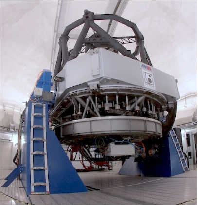
Figure 1: View of the JST/T250 telescope, the primary telescope of the OAJ. It is the telescope used for the miniJPAS  survey, with the JPAS-Pathfinder camera integrated at the Cassegrain focus.

Table 1: Main technical characteristics of the JST/T250 telescope

Mount:	Altazimuthal
Optical configuration:	Ritchey Chrétien modified,
	equipped with a field corrector
	and rotator
M1 diameter:	2.55 m
Field corrector:	3 aspherical lenses
Effective collecting area:	3.75 m2
Focus:	Cassegrain
F$\#$:	3.5
Focal length:	9098 mm
Plate scale:	22.67 arcsec mm-1
FoV (diameter)	3.0 deg
Étendue:	26.5 m2deg2
EE50 (diameter, as-built)	$12\,\mu{\rm m}$
EE80 (diameter, as-built)	$25\,\mu{\rm m}$

The main scientific instrument of the JST/T250, which will be used to carry out J-PAS, is the Javalambre Panoramic Camera (JPCam, Taylor et al. 2014; Marín-Franch et al. 2017), a 1.2 Gpixel camera with an effective FoV of 4.2 deg² and a plate scale of 0.23 arcsec pix^-1. JPCam has completed the assembly, integration and verification phases and is currently being installed and commissioned at the Cassegrain focus of the JST/T250 telescope. Before the arrival of JPCam, the JST/T250 telescope has been equipped with a first light instrument, single CCD camera, called JPAS-Pathfinder, specifically built to test the system optical performance and carry out the first scientific operations.

2.2 The JPAS-Pathfinder camera

The JPAS-Pathfinder camera (JPAS-PF hereafter) is the first scientific, interim instrument installed at the JST/T250 telescope. This single CCD, direct imager had been developed with two primary goals: (i) to minimize the time and risk of JPCam commissioning at the telescope, as it was used to perform the JPCam Actuator System commissioning at the telescope before the JPCam instrument was assembled in the OAJ clean room, and (ii) to start the scientific operation of the JST/T250.

The JPAS-PF camera is equipped with one large format, 9.2k x 9.2k, 10 $\mu$m pixel, low noise detector from Teledyne-e2V located at the center of the JST/T250 FoV. The detector is read out from 16 ports simultaneously. It has an image area of 92.16 mm $\times$ 92.32 mm and a broadband anti-reflective coating for optimized performance from 380 nm to 850 nm. The JPAS-PF consists of two main subsystems, the filter and shutter unit (FSU) and the cryogenic camera.

The cryogenic camera is a 1110S CCD camera manufactured by Spectral Instruments (USA). It comprises the scientific detector and its associated controllers, the cooling and vacuum systems and the image acquisition electronics and control software. The proximity drive electronics provide 16 different operational modes. The miniJPAS survey has been observed with a read mode that achieves total system level noise performance of 3.4 ${\rm e}^{-}$ (RMS), allowing read out times of 12 s (full frame) and 4.3 s (2x2 binning). The FSU includes a two-curtain shutter provided by Bonn-Shutter UG (Germany) that allows taking integration times as short as 0.1 s with an illumination uniformity better that 1$\%$ over the whole JPAS-PF FoV. The FSU incorporates a single filter wheel designed to integrate 7 different J-PAS filters simultaneously. As these filters have a physical dimension slightly smaller than the size of the CCD, the CCD is vignetted on its periphery (see Sect. 3.1). As a result, JPAS-PF provides an effective FoV of 0.27 deg² with a pixel scale of 0.23 arcsec pixel^-1. A summary of the technical characteristics of the camera is presented in Table 2.

The JPAS-PF camera was dismounted at the end of 2019, leaving room for JPCam.

Table 2: Main technical performances of the JPAS-Pathfinder camera

CCD format	$9216\times 9232$ pix
	$10\,\mu{\rm m}\,{\rm pix}^{-1}$
Pixel scale	$0.23$ arcsec pix-1
Effective FoV	$0.54\deg$ $\times$ $0.50\deg$ $=$ $0.27\deg^{2}$
Read out time	12 s (full frame)
	4.3 s (2x2 binning)
Read out noise	$3.4\,{\rm e}^{-}\,{\rm pix}^{-1}$
Full well	$123\,000\,{\rm e}^{-}$
CTE	0.99995
Dark current	$0.0008\,{\rm e}^{-}\,{\rm pix}^{-1}\,{\rm s}^{-1}$
Quantum Efficiency	$40\%$ $@$ 350nm
”	$86\%$ $@$ 400nm
”	$93\%$ $@$ 500nm
”	$93\%$ $@$ 650nm
”	$61\%$ $@$ 900nm
Filters per filter wheel	7

2.3 The J-PAS filter system

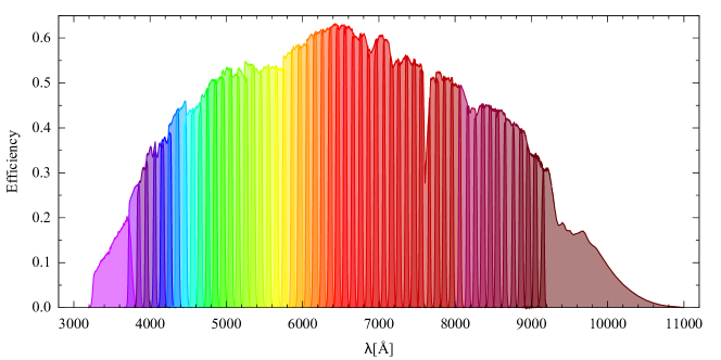
Figure 2: The measured transmission curves of the J-PAS filters. Effects of the CCD quantum efficiency, the entire optical system of the JST/T250 telescope and sky absorption are included. The HTML color representation of each filter is provided in the miniJPAS database in the table minijpas.Filter.

The novel and unique aspect of J-PAS lies on its filter system: $54$ narrow band filters ranging from $3780$ Å to $9100$ Å, complemented with two broader filters in the blue and red wings. The NB filters have a FWHM of $145$ Å and are spaced by about $100$ Å (except for the filter $J0378$), thus creating a continuous spectral coverage through the entire optical range. The two additional filters are one medium band covering the UV edge ($J0348$, called $u_{\rm JAVA}$) and a broad filter red-wards of $9100$ Å ($J1007$). Table 3 lists the main characteristics of the J-PAS filter set, while Fig. 2 shows the transmission curves of the 56 filters described above, where the overall system efficiency has been taken into account (including the atmospheric transmission, the CCD efficiency, and the telescope optics). This filter system effectively delivers a low-resolution ($R\sim 60$) spectra (J-spectra  hereafter) for every object observed and has been particularly designed and optimized to achieve a photometric redshift (photo-$z$) accuracy sufficient to carry out cosmological experiments using a variety of tracers at different redshift ranges (see Benítez et al. 2009, 2014, and Sect. 4.2.2). The observations in the $56$ filters discussed above are complemented with broad-band observations. The miniJPAS field has been observed with the SDSS-like broad band filters $u_{\rm JPAS}$, $g_{\rm SDSS}$, $r_{\rm SDSS}$, and $i_{\rm SDSS}$. The $r_{\rm SDSS}$ filter has been chosen as the detection band for the miniJPAS “dual-mode” catalogues, as explained in Sect. 3.4. From now on, unless otherwise stated, we will refer to these filters simply with $u$, $g$, $r$ and $i$. The information on FWHM and central wavelengths of these filters is also available, as for the other filters, in the miniJPAS data release ADQL table minijpas.Filter (see Sect.4.3). The filter transmission curves are publicly available at the Spanish Virtual Observatory page.

Beyond the specified theoretical filter transmission curves, whose definition is exclusively driven by the main scientific goals, additional functional requirements are influenced by the telescope and instrument opto-mechanical designs. Some of the most demanding requirements are: filter physical dimension (101.7 mm $\times$ 96.5 mm), central wavelength (CW) uniformity across the filter usable area (CW varies less than $\pm$ 0.2$\%$), high band-pass transmission and flatness (higher than 90$\%$, except for the bluest filters, with a flatness better than 5$\%$ peak-to-valley), out of band blocking (OD5 from 250 to 1050 nm) and filter-to-filter continuity (overlap at transmissions higher that 75$\%$).

The J-PAS filters have been designed by CEFCA and SCHOTT Suisse SA (Switzerland) and manufactured by SCHOTT. A detailed technical description of the filter requirements, design, measurements and characterization can be found in Marin-Franch et al. (2012), Brauneck et al. (2018a) and Brauneck et al. (2018b).

Table 3: Filter system main characteristics. The full table is available in the miniJPAS database in the ADQL table minijpas.Filter.

		Central
Filter $\#$	Filter name	Wavelength	FWHM
		[Å]	[Å]
1	$uJAVA$	3497	495
2	$J0378$	3782	155
3	$J0390$	3904	145
4	$J0400$	3996	145
5	$J0410$	4110	145
$...$	$...$	$...$	$...$
54	$J0900$	9000	145
55	$J0910$	9107	145
56	$J1007$	9316	High-pass filter

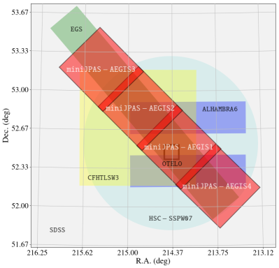
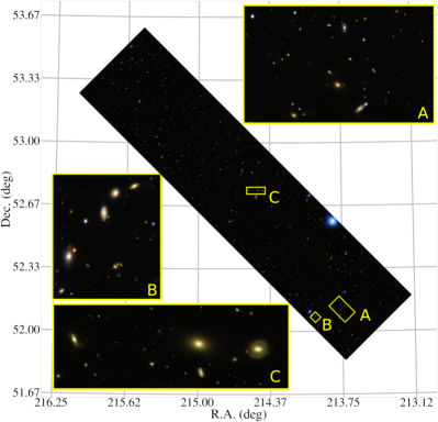
Figure 3: Left: Footprint of the miniJPAS field, with pointings shown as red squares (see their coordinates in Table 4). It overlaps with the footprints of other projects, also shown for reference: EGS (in green), pointing #6 of the ALHAMBRA Survey (in violet), the W07 wide field of the HSC-SSP (large circle in pale blue), field W3 of the CFHTLS (in yellow), OSIRIS Tunable Emission Line Object survey (OTELO) (small square close to the center of the figure) and SDSS (in light gray occupying the whole area). We refer to Table 9 for the references to these overlapping surveys. Right: $g,r,i$ color image of miniJPAS  with zoom in three selected areas.

2.4 miniJPAS observations

This section is devoted to the description of the miniJPAS observations, from the definition of the footprint to the observational strategy and the primary statistics of the collected data.

2.4.1 Footprint and survey strategy

The area targeted for the miniJPAS observations is the well-known EGS field, in the north galactic hemisphere. The field has been chosen for two main reasons: (i) its sky location ($+215.00$^∘,$+53.00$^∘), which makes it optimally observable at altitudes $>30$^∘ from the OAJ from February to July and (ii) the wealth of multi-wavelength data available in the field, from the AEGIS project, to SDSS and the HSC-SSP wide field. The size of the JPAS-PF camera FoV allowed to cover the EGS field almost entirely with only $4$ pointings, with observations carried out with the instrument rotated at $45$^∘ with respect to the celestial North. The $4$ pointings composing the miniJPAS field are listed in Table 4 and shown in Fig. 12, together with the footprints of other projects.

The overlap between the pointings is of $3.6$′. Each tile was covered with a minimum of $4$ exposures, with a dithering of $10$ arcsec along the horizontal and vertical direction of the CCD. The total area covered is $\sim 1\deg^{2}$, while the total area with overlapping tiles is $\sim 0.09\deg^{2}$, $9\%$ of the total area. After taking the mask into account, the effective area is $0.895\deg^{2}$ (see Sect. 3.6).

The exposure times for the miniJPAS observations have been scaled up with respect to the ones quoted in Benítez et al. (2014) to account for the degraded reflectivity of M1 during observations. For the $56$ J-PAS filters and the $u$ filter, each independent exposure was of $120\sec$, while each exposure for the broad bands $g$, $r$ and $i$ was of $30\sec$, to avoid saturation. The basic strategy for the narrow bands and $u$ required $4$ exposures, one per dithered position (except for the reddest filters, where a minimum of $8$ exposures, two per dithered position, was planned), while the strategy for the broad bands was of $4$ exposures per dithered position. Therefore, the total minimum exposure time per filter was set to $480\sec$, $4\times 120\sec$ for the NB and $u$ ($960\sec$ for the reddest filters ) and $4\times 4\times 30\sec$ for the BB. However, for several filters more than this minimum number of images is currently available, as multiple observations have been carried out with different sky conditions to test the system. Concerning the readout modes, the same setup expected for J-PAS was adopted: full frame mode for $u$, $g$, $r$, $i$ and 2x2 binning for the remaining filters. The readout noise is the same in the two cases (see Table 2). All good-quality images (see Sect. 3) have been included in the coadded images used to generate the miniJPAS catalogues. The number of exposures available per filters and per tile are provided in Appendix A. The resulting depths are shown in Fig. 4. The minimum target depths are reached in all the filters, with most actually reaching fainter magnitudes. The differences in depth from band to band depend both on the net effect of sky brightness when the observations were acquired and on the final number of combined images. This inhomogeneity is expected to be minimized for J-PAS data, as the exposure times for each pointing will be modulated according to the sky brightness of the night, following a similar procedure than the one applied in J-PLUS (Cenarro et al. 2019).

Table 4: Central coordinates of each pointing.

Tile	RA J2000 (deg)	DEC J2000 (deg)
miniJPAS-AEGIS1	214.2825	52.5143
miniJPAS-AEGIS2	214.8285	52.8487
miniJPAS-AEGIS3	215.3879	53.1832
miniJPAS-AEGIS4	213.7417	52.1770

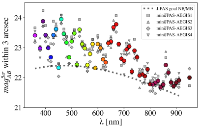
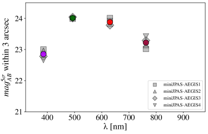
Figure 4: Estimated depths ($5\sigma$ at $3$ arcsec aperture), computed from the noise in each tile, for the narrow bands (left) and broad bands (right). The coloured symbols show the average values for each filter, while the gray ones are the values for the co-added images of each pointing. For the narrow bands, the dashed gray line indicates the approximate targeted minimum depth, as defined in Benítez et al. (2014).

2.4.2 Details on data acquisition

Data were acquired between May and September 2018, although for few filters further images were taken in the next available season in 2019 (see Appendix A). Because of the nature of the filter wheel available for the JPAS-Pathfinder camera (see Sect. 2.2), observations were performed in groups of six filters. The filter ordering was chosen to maximize the data validation and scientific analysis as the survey was progressing, and to ensure a broad enough spectral coverage in case some filters could not be observed for unforeseen reasons. Even though the nominal desired minimum elevation of the telescope during observations is $40^{\circ}$, for this first data set this restriction was relaxed to allow observations for a longer period of time. The quality of the data in terms of PSF and depth suffered only mildly from this choice, as images with FWHM below $2$ arcsec can be taken down to an elevation of around $30^{\circ}$.

The average FWHM per tile and per filter are shown in Fig. 5. Most of the bands have FWHM below $1.5$ arcsec. A slight systematic increase in FWHM can be observed for the reddest bands, from $800$ nm up and, especially, from $860$ nm to higher wavelengths. The main reason for this behaviour is that the reddest filters were scheduled to be observed last, and towards the end of the observing campaign the EGS/AEGIS field reached the lowest elevations. As a consequence, the FWHMs are larger than the ones we would have obtained at lower zenith distances with the same atmospheric conditions. Nonetheless, very few tiles have PSFs with FWHM above $2$ arcsec. Regarding the 2D stability of the PSF across the images, the median rms FWHM relative variation is, accounting for all filters and tiles, $3.7\%$, with a normalized median absolute deviation, $\sigma_{NMAD}$, of 2.3%.

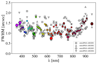
Figure 5: Statistics of the PSF FWHM. The coloured symbols represent the average values for each filter, while the gray ones are the value for each pointing. The larger symbols indicate the FWHM of the the broad bands.

3 The J-PAS pipeline and data management

All data collected by the OAJ observatory are handled and processed by the Data Processing and Archiving Unit (hereafter UPAD) group at CEFCA. The UPAD data center (Cristóbal-Hornillos et al. 2014) has the capacity to provide reduced and calibrated data and to archive and allow external access to the whole scientific community. In this section we go over the several steps of data managing, from the construction of coadded images to the development of the source catalogues.

3.1 Processing of single frames

The detrending of the single frames follows the standard steps of bias subtraction, pre/overscan subtraction, trimming, flat field correction, illumination correction and, if needed, fringing corrections. We refer to  Cenarro et al. (2019) for details on how these steps have been implemented, as the same procedure as for J-PLUS has been followed. In what follows we focus on few particular aspects that needed specific treatment for miniJPAS  data (e.g., reflections, background patterns, etc.), provided that JPAS-PF was not specifically designed for JST/T250 and its FoV is significantly smaller than the one of the telescope. For the same reason, we do not expect many of these issues in the final J-PAS images from JPCam, since both camera and the telescope were designed together as a unique optical system.

The main issues that needed special treatment were:

Vignetting.

The first detected issue on JPAS-PF images is a strong vignetting in the outer parts of the CCD. As a result, the images show a strong gradient of efficiency. To minimize the impact on the final measurements, the images need to be trimmed to exclude regions with low efficiency. The preliminary tests required a reduction of the effective area of the CCD from 9216 $\times$ 9232 pixels to 7777 $\times$ 8473. The resulting effective FoV of JPAS-Pathfinder is thus 0.27 deg² (see Table 2).

Background patterns.

The other important issue detected in JPAS-PF images are background patterns with strong gradients and variations in time scales of few minutes, which affect in different ways filters at different wavelengths. We were able to identify two kinds of reflections with two different origins. The first one is characterized by straight patterns and is likely due to the optics of the camera. The second one, instead, features circular patterns affecting many of the reddest filters, likely due to the small variation of the central wavelength of the transmission curves of the filters. In both cases, the net effect is an irregular distribution of the sky light which affects the images in two ways: affecting the flat field images via spurious changes of efficiency and creating an irregular background pattern. The first needs to be corrected through the illumination correction while the second needs a careful subtraction to not affect the photometry of the objects.

The technical details of the procedures followed to remove the background patterns can be found in Appendix B. The left panels of Fig. 6 show an example of an image before and after the background subtraction.

Fringing.

For filters redder than J0740, the presence of fringing requires an extra step to remove the pattern. In this case, we follow the standard implementation already used for the $z$ filter of J-PLUS and constructed master fringing images using all available images taken with JPAS-PF in each filter. This is possible as the fringing pattern is very stable across nights. However, some small residuals of the fringing pattern could still be visible in the final images of a few filters for which the pattern can be particularly strong (special mention here for the J1007 filter), and for which the number of available images is small.

The right panels of Fig. 6 show an example of an image of the J0880 filter before and after full processing. In the raw image one can see vignetting in the edges, present in all the images, and the circular pattern and fringing, which are common in the red filters.

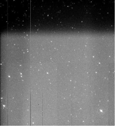
(a) Example of an image before and after background subtraction (miniJPAS-AEGIS2, in the filter J0690).

(b) Example of an image before and after the full processing (miniJPAS-AEGIS1, in the filter J0880).

Figure 6: Examples of image processing. In the left panels, an example of the background subtraction. In the right panels, an example of the full processing, from a raw image to the final one.

Astrometric calibration is the last step needed for the proper combination of the images. This is carried out again as a part of the standard procedure for OAJ images using the software Scamp (Bertin 2010a) and the Gaia DR2 (Gaia Collaboration et al. 2018) as reference catalogue. The typical uncertainty of the final astrometry of the single frames, with respect to Gaia, is $\sim 0.035$ arcsec. That is a small fraction ($\sim 7-15\%$) of the pixel size, which is $\sim 0.23$ arcsec for not binned images and $\sim 0.46$ arcsec for the binned ones.

3.2 Final coadded images

Once the single frames are cleaned of instrumental effects, they are combined with the Astromatic software Swarp (Bertin 2010b). All the images are sampled to the fiducial pixel size of the camera (i.e., $0.23$ arcsec pixel^-1), including all the images of the narrow bands that were observed with a binning of 2$\times$2. We opted for keeping the orientation as the one of the original frames instead of forcing to have the coadded images oriented with North towards up (increasing Y axis) and East toward left (decreasing X axis). In addition to the combined scientific images, Swarp also constructs a normalized weight image that keeps track, for example, of areas were the number of combined images is lower (for instance, in the edges due to the dithering pattern but also in regions were spurious detection were previously masked in one or more single frames). Therefore, the weight image can be considered as a map of the effective exposure time of the different parts of the image. This is taken into account, for example, in the masking process explained below, in Sect. 3.6.

3.3 PSF treatment

One of the main challenges of large field surveys is to provide homogeneous photometry for a large number of objects. Each miniJPAS pointing is composed of 60 coadded images from multiple exposures. Variations in the PSF from filter to filter can produce inhomogeneous photometry, thus artificial color terms, since the light coming from the same area of the sky will be redistributed differently in the final image depending on the filter used.

This discontinuous PSF variations can cause problems in the photometry for objects with a significantly different PSF between the tiles. The homogenization process allows PSF-Matched aperture-corrected photometry measurements to be more consistent, at the expense of degrading some images (see Sect. 3.4). This method uses PSFEx (Bertin 2011) to calculate a PSF homogenization kernel, to convert variable instrumental PSFs to constant round Moffat profiles for practical purposes. The homogenization process has consequences in the image noise and generates variable noise correlations over the image pixels. For that reason, the algorithm recalculates the noise model of the images that later is used to compute photometric errors (Molino et al. 2014). We only apply the homogenization kernel to the corrected PSF apertures (PSFCOR and WORST_PSF, see Sect. 3.4) in the dual-mode catalogues, while for all other apertures no convolution takes place.

As product of the PSF analysis of the images, we provide the overall PSF model produced by PSFEx for each image, as well as a service that generates on-demand an actual image of the PSF model in any position of any image (see Sect. 4.1.2).

3.4 Photometry

The detection of sources in the images is done with the widely used software SExtractor (Bertin & Arnouts 1996). To cover as much as possible the needs of the astronomical community we have run SExtractor in two different complementary ways:

Dual-mode.

To construct catalogues in which the photometry in the different bands for each object is done consistently, we have run SExtractor in the so called “dual-mode”. In dual-mode, SExtractor is first run on a reference image for source detection and for the definition of the position and sizes of the apertures. Afterwards, it is run on the other images, where the photometry is performed within the apertures defined by the reference image (forced photometry). In our case, we chose the $r$ band co-added images as reference images for constructing the dual-mode catalogues.

Single-mode.

In the so called “single-mode”, both the detection and the photometry are performed for each filter separately. This has the advantage that objects not detected in the reference band (e.g., faint objects with strong emission lines out of the $r$ band) can be identified. The drawback is that, for the same object, the photometry can be done in slightly different positions in the different bands, increasing the chance for inconsistent colours.

The detection parameters were set to particular values to compromise between large detectability (i.e., completeness), while avoiding spurious detections (i.e., purity). Due to higher noise in all the bands different to the $r$ band, the detection threshold (in units of the $\sigma$ of the background) for the generation of single-mode catalogues were set to a higher value (DETECT_THRESH=2) than for the dual-mode catalogues (DETECT_THRESH=0.9). The full list of SExtractor parameters can be found in the Appendix C.

3.5 Photometric calibration

The final step to generate the final catalogues is the photometric calibration of the fluxes. The photometric calibration of miniJPAS data was adapted from the methodology presented in (López-Sanjuan et al. 2019a), developed to provide the calibration of J-PLUS. We applied the following steps:

1. Definition of a high-quality sample of stars for calibration. We selected those miniJPAS+Gaia sources with $S/N>10$ in all the photometric bands and with $S/N>3$ in Gaia parallax. We constructed the dust de-reddened absolute $G$ magnitude vs. $G_{BP}-G_{RP}$ colour using the information from the 3D dust maps in Green et al. (2018a) and selected those sources belonging to the main sequence. This provides 334 calibration stars.

2. Calibration of the $gri$ broad-band filters to the Pan-STARRS photometry. We compared our $6^{\prime\prime}$ aperture magnitudes corrected to total magnitudes with the PSF magnitudes in Pan-STARRS. The aperture corrections were computed from the light growth curves of unsaturated, bright stars in each tile and are stored in the ADQL table minijpas.TileImage. This step provides the zero points of the $gri$ broad band filters. We computed also the zero points by comparison with J-PLUS photometry, obtaining differences below $0.01$ mag.

3. Homogenization of the narrow bands with the stellar locus. For each NB, we compute the dust de-reddened $(\mathcal{X}_{\rm ins}-r)_{0}$ vs. $(g-i)_{0}$ colour-colour diagrams of the calibration stars, where $\mathcal{X}_{\rm ins}$ is the instrumental magnitude of the selected NB. From this, we computed the offsets that lead to a consistent stellar locus among the pointings. This provides a homogeneous instrumental photometry in miniJPAS.

4. Absolute colour calibration. The last step is to translate the instrumental magnitudes on top of the atmosphere. This step was done in J-PLUS with the white dwarf (WD) locus, but there is no high-quality WD in the miniJPAS area. We therefore used BOSS stellar spectra as reference to provide the absolute calibration of miniJPAS  colours. After a visual inspection of the available BOSS spectra, we ended up with 40 stars. We compared the synthetic $(\mathcal{X}-r)$ colours from BOSS spectra with the instrumental magnitudes from miniJPAS to obtain one offset per passband except for $r$, which is used as reference and anchored to the Pan-STARRS calibration.

5. The BOSS spectra do not cover the $u_{\rm JAVA}$ and $u_{\rm JPAS}$ filters. For these bands, we obtained the colour offset by direct comparison with J-PLUS photometry.

Summarising, the flux calibration of miniJPAS photometry is referred to the Pan-STARRS $r$ band and the colours are anchored to the BOSS spectra except for the $u_{\rm JAVA}$ and $u_{\rm JPAS}$, which are anchored to the J-PLUS photometry.

We estimate the zero points also by direct comparison with J-PLUS photometry in the shared or similar passbands. Such comparison provides consistent zero points at the 4% level. Thus, we conclude that the current photometric calibration has an absolute error of $\sim 0.04$ mag. We set this as a safe upper limit in the calibration performance because of the limited statistics to provide an accurate estimation. The consistency in the calibration among tiles is tested in Sect. 5.1 by comparing the photometry in overlapping areas. Note that this comparison only reflects the errors in the miniJPAS homogenization (step iii) and is not sensitive to the uncertainties in the absolute colour calibration (steps iv and v). We expect to reach a 1-2% accuracy in the J-PAS photometric calibration when $\sim 500$ deg² are gathered. This will provide a few hundred WDs to derive a consistent colour calibration with the WD locus and a robust estimation of the uncertainties thanks to a large number of overlapping areas with duplicated measurements of the same sources.

3.6 Masks

In order to help the identification of problematic areas in the images, we also computed masks, provided in the MANGLE format(Swanson et al. 2008). In addition, we flag the objects falling in those masked areas storing this information in the FLAGS_MASK column of the catalogues (see Sect. 4.1.1).

The problematic areas that we are currently identifying and masking are the following:

Window frame mask.

This mask identifies regions where the normalized weight map values are less than 85%. This is determined from the tiling weight-map image, in order to homogenize the effective exposure times for the same coadd. The threshold value has been selected to be a compromise to maximize the valid observation area and minimize regions with less effective exposure time where, usually, a lower number of images have been combined. Nevertheless, for each object we compute the value of the normalized weight map at its position, which is stored in the parameter NORM_WMAP_VAL. This parameter takes a value of 1 in the area with highest effective exposure.

Mask of bright stars.

The mask of bright stars discards regions around bright stars found in the Bright Star Catalog and the Tycho-2 catalog (Høg et al. 2000). The radius of each masked region is a function of the magnitude of the star.

Mask of artefacts.

This mask identifies obvious artefacts in the images, usually due to light reflections in the telescope or its optical elements. We developed specific algorithms able to automatically detect, analyse and mask artefacts or patterns. In addition, artefacts not detected automatically are manually masked.

We provide the masks for each tile or coadded image as well as a combined mask of the whole miniJPAS footprint.

4 The miniJPAS data set and data access

In this section we describe the data products available and how to access them.

4.1 Data products

This data release includes images, basic catalogue data (parameters measured from images, such as photometry or morphology data), as well as value-added information.

For images we provide not only the final coadded image but also the following ancillary data:

• Basic parameters of the observations, like total exposure time, photometric zero points, estimations of the photometric depth, etc.

• Information on the single frames used for generating the co-added image, including the details of the sky conditions during the observations.

• The weight image resulting from the Swarp co-adding procedure (see Sect. 3.2).

• Mask (see Sect. 3.6).

• PSF model as resulting from PSFEx (see Sect. 3.3).

The information of individual objects or detections is placed in different tables in a relational database. We provide two kinds of tables storing the data coming from running SExtractor in both, “dual-mode” and “single-mode”, as explained in Sect 3.4. For the dual-mode, the photometry of each detection in all the bands is unique by construction. In the catalogues, for each detection in the reference band, we provide the list of geometrical parameters (position of the barycentre, shape, FWHM,…) as well as different types of photometric measurements in all the bands. For the single-mode, the relation between measurements in different bands is not always straightforward and the actual identification of measurements in different bands will depend on the strategy for the cross-matching between catalogues. Therefore, we opted for providing a catalogue with all the detections treated independently leaving to the user the freedom to perform the cross-match in the most convenient way.

In summary, each entry in the dual-mode catalogue corresponds to one object detected in the $r$ band and its photometry in all the J-PAS bands while each entry in the single-mode catalogue is a detection of one object in one band (and only if it is detected in that band) and, hence, each detection in each band has its own entry in the single-mode catalogue. Table 5 shows a brief summary of the basic number counts for each pointing and for dual- and single-mode catalogues.

To cover the needs of different kinds of analyses, we provide the photometric catalogues in three different units:

• AB magnitudes (names of the tables tagged with MagAB).

• Fluxes as a function of wavelength in units of $10^{-19}$erg s${}^{-1}\,$cm${}^{-2}\,\AA^{-1}$ (names of the tables tagged with FLambda).

• Fluxes as a function of frequency in units of $10^{-30}$erg s${}^{-1}\,$cm${}^{-2}\,$Hz^-1 (names of the tables tagged with Fnu.).

Table 5: Detected objects for each miniJPAS pointing. N_Dual refers to the total number of detections in the dual-mode catalogues as derived by SExtractor (see Sect. 3.4 and SExtractor parameters in Appendix C). N_Single refers to the total number of detections in the single-mode catalogues. Note that for the single-mode catalogues a higher detection threshold for SExtractor has been applied (see Sect. 3.4).

Pointing	NDual	NSingle
miniJPAS-AEGIS1	20016	167150
miniJPAS-AEGIS2	13836	142481
miniJPAS-AEGIS3	15792	142496
miniJPAS-AEGIS4	14649	152443
Total	64293	604570

We detail the different types of photometry that are provided in the database:

MAG_AUTO, MAG_ISO, MAG_PETRO.

These are different types of estimations of total magnitudes. The reader is referred to SExtractor User’s Manual for a detailed description.

MAG_APER_....

These correspond to aperture photometry in apertures of different sizes. The numbers in the names refer to the sizes of the aperture in arcseconds, e.g. MAG_APER_1_5 corresponds to the photometry in an aperture of 1.5 arcsec of diameter.

MAG_ISO_WORSTPSF, MAG_APER3_WORSTPSF.

These correspond to MAG_ISO and MAG_APER_3_0 with the particularity of being measured after transforming all the images of a given pointing to present a PSF size equal to the worst PSF among all the images. This is a straightforward procedure to remove the effect of the variation of the PSF among different filters on the photometry and to have more robust measurements of the colours. The disadvantage is the loss of information from the images with better PSF.

MAG_PSFCOR.

This photometry is performed following the approach of Molino et al. (2019) (see also Molino et al. 2014, 2017) with the aim of applying corrections object by object in the images with worst PSF to correct for the differences in PSF among different bands. To increase the robustness of the color determination, instead of total magnitudes estimators like MAG_AUTO or MAG_ISO, the fluxes are measured within an aperture with the same shape as the Kron aperture and a semimajor axis equal to 1 KRON_RADIUS, also called restricted magnitudes (Molino et al. 2017, 2019). Being smaller than the aperture of MAG_AUTO, the signal-to-noise ratio is higher and, therefore, color measurements, which are key in spectral analysis like photo-$z$ determination, are more robust. We stress, though, that these are not total magnitudes.

Table 6: List of individual MASK_FLAGS values. The final value of the MASK_FLAGS parameter of a given object will be the sum of all the individual MASK_FLAGS flags that apply to that object.

Value	Name	Description
0	not mask	Not inside a mask
1	window	Object is outside the window frame
2	bright star	Object is bright star or near one
4	artefact	Object masked due to nearby artefact

4.1.1 Flags

In order to easily identify objects with known specific issues, for each detected object two types of flags are provided to help in that identification.

SExtractor FLAGS.

This parameter, inherited from SExtractor, contains 10 flag bits with basic warnings about the source extraction process (see Table 7). To the original first 8 flags from SExtractor, the values 1024 and 2048 have been added to identify, respectively, objects with detections in more than one image (in the area where tiles overlap) and known variable objects from the cross-match with other surveys. Like in SExtractor, the final value of the FLAGS parameter of a given object is the sum of the individual values of the FLAGS that affect that object.

Table 7: List of individual FLAGS values. The final value of the FLAGS of a given object will be the sum of all the individual FLAGS values that apply to that object.

Value	Name	Description
1	close neighbours	The object has neighbours, bright and close enough to significantly bias the photometry, or bad pixels (more than 10% of the integrated area affected)
2	blending	The object was originally blended with another one
4	saturation	At least one pixel of the object is saturated (or very close to saturation)
8	truncated	The object is truncated (too close to an image boundary)
16	aperture incomplete	Object’s aperture data are incomplete or corrupted
32	isophotal incomplete	Object’s isophotal data are incomplete or corrupted
64	memory overflow deblending	A memory overflow occurred during deblending
128	memory overflow extraction	A memory overflow occurred during extraction
1024	duplicated	The object has been marked as duplicated
2048	known variable	The object could be a known variable

Mask FLAGS.

Besides the issues affecting individual objects, there are large areas of the images affected by different problems. Those areas are identified and masked (see Sect. 3.6) and the objects falling inside those masked areas are flagged using the MASK_FLAGS parameter. In Table 6 are shown the individual values that the MASK_FLAGS parameter can have and the corresponding image issues. Like in the case of the FLAGS parameter, the final value of the MASK_FLAGS parameter for each object is the sum of all the individual MASK_FLAGS that applied to that object.

4.1.2 PSF models

In Sect. 3.3 we described how we treated variations of the PSF from filter to filter to achieve a homogeneous photometry. In the database the PSF models are provided in two different ways:

• As the direct output of PSFEx. This can be downloaded for each image through the “Image Search” service of the Web Portal.

• As FITS images of the actual model of the PSF for a given position in a given image. This is an “on-demand” service accessible via HTTP request to allow programmed access.

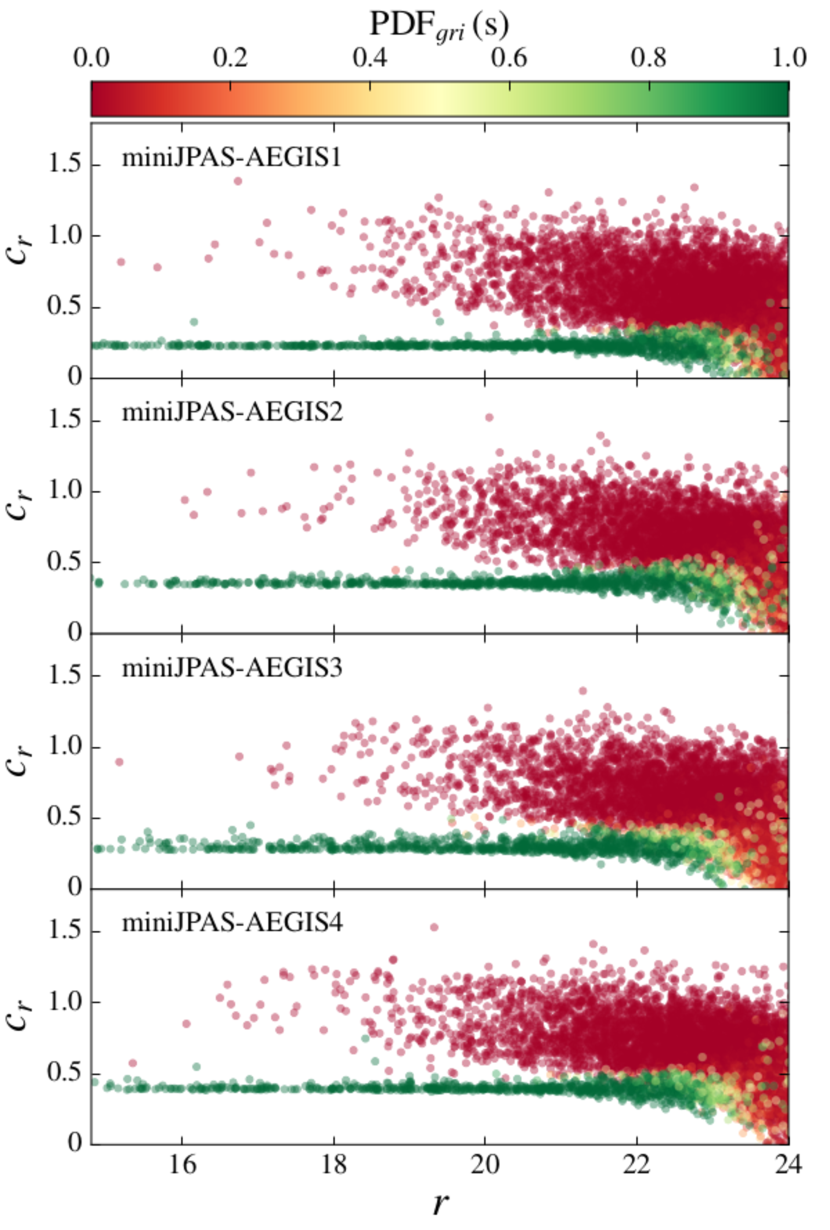
Figure 7: Concentration-magnitude relation (MAG_AUTO) for sources in each individual miniJPAS pointing. Symbols are color-coded according to the probability of being compact or extended, based on the SGLC of López-Sanjuan et al. (2019b), adapted to miniJPAS data.

4.2 Value-added catalogues

On top of the basic photometric information described above, the database contains a wealth of ancillary information to facilitate the scientific analysis of the data. We describe the most relevant ones below.

4.2.1 Stellarity index

The database provides the results of different complementary methods for the star/galaxy classification of the sources, where “stars” are considered all compact/point-like objects (thus including quasars and very compact galaxies) and “galaxies” all resolved ones. We provide here a brief description of the three approaches:

SExtractor classification

SExtractor automatically provides a morphological classification (the CLASS_STAR parameter) for all detected objects. We refer to the manual of SExtractor for details on this classification.

Stellar-Galaxy Locus Classification (SGLC)

We applied the Bayesian star/galaxy morphological classifier developed in López-Sanjuan et al. (2019b) for J-PLUS data. The concentration vs. magnitude diagram presents two distinct populations, corresponding to compact and extended sources (see Fig. 7). We modelled both populations to obtain for each source a probability for being compact or extended, as indicated in Fig. 7 by the color of the symbols. The most relevant update with respect to the J-PLUS methodology is the modification of the galaxy population model. The galaxy locus is assumed to be constant with magnitude in the J-PLUS analysis, but such assumption does not hold at the fainter magnitudes probed by miniJPAS data. Galaxies become apparently smaller at larger magnitudes, with the galaxy locus approaching asymptotically to the stellar locus. We modelled such trend with an error function calibrated with miniJPAS data. The morphological information in the $g$, $r$ and $i$ broad band filters was combined. A prior in $r$ magnitude, accounting for the larger number of galaxies at fainter magnitudes and estimated in each pointing independently, was applied. The modelling of the stellar and galaxy populations was done pointing-by-pointing as in López-Sanjuan et al. (2019b). As we will show in Sect. 5.4, the number counts derived from this Bayesian classification agree with the expectations from the literature up to $r\sim 23.5$. The derived probabilities for the morphology of each source are publicly available in the ADQL table minijpas.StarGalClass.

Machine learning classification

We used machine learning (ML) to classify sources of miniJPAS as stars or galaxies in the magnitude interval $15\leq r\leq 23.5$. In order to train and test our classifiers, we cross-matched the miniJPAS dataset with SDSS and HSC-SSP data, whose classification we assume to be trustworthy within the intervals $15\leq r\leq 18.5$ and $18.5<r\leq 23.5$, respectively. The best ML classifiers are Extremely Randomized Trees (ERT) and Random Forest (RF), whose performance is shown in Fig. 8 as compared to SExtractor and SGLC, described above. We can see that, when using morphological parameters, ERT outperforms SGLC. For the case in which we use only photometric bands, RF is the best classifier. For a more detailed analysis with other methods and metrics see Baqui et al. (2020). A value added catalogue is available in the miniJPAS database via the ADQL table minijpas.StarGalClassML

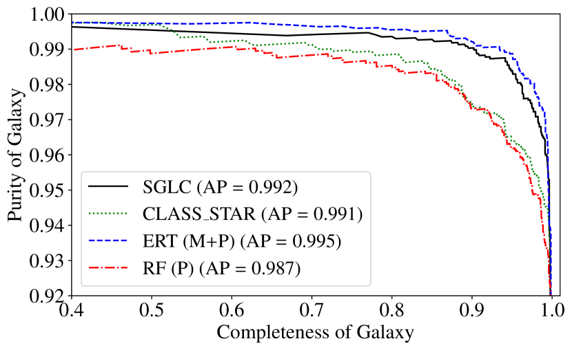
Figure 8: Purity-completeness curves for galaxies in the magnitude range $15\leq r\leq 23.5$, based on the morphological classification of SExtractor (CLASS_STAR, green dotted line), SGLC (black solid line), Extremely Randomized Trees (blue dashed line) and Random Forest (red dot-dashed line). ERT uses both the photometric (P) and morphological (M) information of the sources, while the RF uses photometric information only.

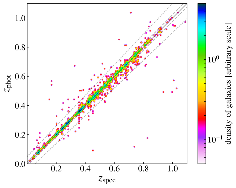
Figure 9: Comparison between photometric and spectroscopic redshifts for miniJPAS galaxies at $r<22.5$ with ODDS¿0.5. In order to better highlight the density of points, we have applied a 2-D Gaussian smoothing to the data. The solid line marks the 1:1 relation. The two dashed lines enclose a region containing $80\%$ of the sources, while the dotted lines indicate the $\lvert\Delta z\rvert=0.05$ threshold used to define redshift outliers. Note that each outlier smoothed regions correspond to individual sources.

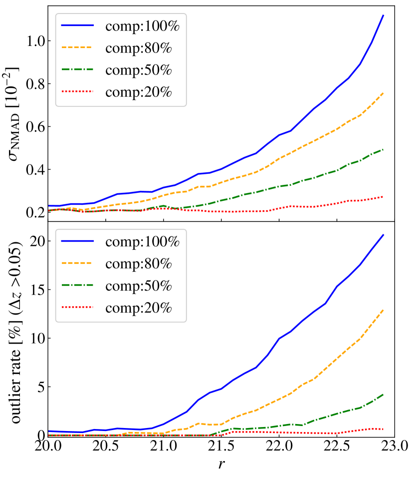
Figure 10: Normalized median absolute deviation of photo-$z$ errors (top panel, in units of $[10^{-2}]$) and outlier rate (bottom panel) as a function of the limiting magnitude in the $r$-band (MAG_AUTO). Outliers are defined as having redshift errors $\lvert\Delta z\rvert$ $>$ 0.05. The colors refer to different cuts in the ODDS parameter, resulting in the selection of 100%, 80%, 50% or 20% of the sources in the spectroscopic sample. The $\sigma_{\rm{NMAD}}$ values and the associated errors are provided in Table 8.

4.2.2 Photometric redshifts

The photometric redshifts (photo-$z$) for miniJPAS were obtained with the jphotoz package, developed at CEFCA as part of the reduction pipeline for the J-PLUS and J-PAS surveys. jphotoz is a set of python scripts that acts as interface between the database and the actual photo-$z$ computing code, which is a custom version of LePhare (Arnouts & Ilbert 2011) modified to work with a larger number of filters and higher resolution in redshift than typically required for broadband photometry.

LePhare computes photo-$z$ by fitting the observed photometry of each source with a set of templates. We used 50 galaxy templates specifically tailored for miniJPAS data. The templates are stellar population synthesis models generated with CIGALE that match the J-spectra of individual miniJPAS galaxies. The process of generation and selection of the most suitable set of templates is described in detail in Hernán-Caballero et al. (in prep.).

To test the accuracy of miniJPAS photo-$z$ we use a subsample of galaxies with spectroscopic redshifts taken from SDSS DR12 and the DR4 of the DEEP2 Galaxy Redshift Survey (Newman et al. 2013). The later covers the footprint of the EGS and includes $12,051$ reliable galaxy redshifts down to magnitude $r=24.1$, with no preselection in magnitude or colour. We matched sources in the miniJPAS catalogue with those in SDSS and DEEP2 using a search radius of 1.5 arcsec. To ensure a proper evaluation of the photo-$z$ accuracy in galaxies, we considered only sources with a reliable redshift determination (Q ¿= 3 in DEEP2 or zwarning = 0 in SDSS) and spectroscopic classification as galaxy. In addition, we excluded sources with FLAGS¿0 in the miniJPAS photometric catalogue. Table 8 summarizes the total number of miniJPAS sources and the number of those used for evaluation of the photo-$z$ accuracy in bins of magnitude.

The error in the photo-$z$ for a given source is expressed by the quantity $\Delta z=(z_{\rm{phot}}-z_{\rm{spec}})/(1+z_{\rm{spec}})$. The distribution of $\Delta z$ is approximately Gaussian but with heavier wings far from the core due to an almost flat distribution of outliers (defined as those galaxies with catastrophic redshift errors $\lvert\Delta z\rvert$ $>$ 0.05) in the redshift search range. A common statistic used to represent the width of the distribution is the normalized median absolute deviation $\sigma_{\rm{NMAD}}=1.4826\times{\rm median}(\lvert\Delta z-{\rm median}(\Delta z)\rvert)$, which equals the standard deviation for a purely Gaussian distribution but is less sensitive to the outliers.

It is possible to select samples with more accurate photo-$z$ (both in terms of $\sigma_{\rm{NMAD}}$ and outlier rate) by sacrificing the sources with the least reliable estimates. Our confidence in the photo-$z$ determination of individual sources depends on the shape of their redshift probability distribution function (PDF). A common parametrization of this confidence is the ODDS parameter (Benítez 2000), defined as the integral of the PDF in a window of fixed width centred at the mode of the PDF. For miniJPAS, we choose a half-width of $0.03(1+z)$ for the integration window. The value of the ODDS ranges from  0 to 1, with higher values implying higher confidence in the photo-$z$.

In Fig. 9 we show the photometric vs. spectroscopic redshift plane for the sources at $r<22.5$ with ODDS¿0.5, which qualitatively indicates the high level of precision of our photo-$z$ solutions. The redshift precision for this sample is $\sigma_{\rm NMAD}=0.004$ and the outlier rate $\sim 4\%$.

In Fig. 10 we show the $\sigma_{\rm{NMAD}}$ and outlier rate for the sample with spectroscopic counterparts as a function of the limiting magnitude in the $r$ band, after applying cuts in ODDS corresponding to completeness of 20, 50, 80 and 100%. As expected, both $\sigma_{\rm{NMAD}}$ and the outlier rate increase for fainter magnitude cuts due to the decrease in the average S/N of the J-spectra. For the entire sample of 2421 galaxies at $r<22.5$ with reliable spectroscopic redshifts, we obtain $\sigma_{\rm{NMAD}}=0.0078\pm 0.0004$ and an outlier rate of $15.3\pm 8\%$ (for $\Delta z=0.05$), where the uncertainties are calculated using bootstrap resampling. However, it is possible to select subsamples with $\sigma_{\rm{NMAD}}$ as low as $\sim 0.002$ and an outlier rate of $\sim 1-2\%$ just by imposing a more restrictive cut in ODDS. We note that further refinement of the photometry might lead to even better photo-$z$ depth. The threshold value of the ODDS parameter required to achieve the desired redshift accuracy or completeness is shown in Fig. 11. In Sect. 6.3 we show how different cuts in ODDS translate to cuts in number densities and redshift precision for sources at different redshifts.

Table 8: Redshift precision, in units of $[10^{-2}]$ for different magnitude cuts, differential and cumulative, and for different completeness cuts ($100\%$, $80\%$, $50\%$ and $20\%$)

$r$ (MAG_AUTO)	Ntot	Nused	$\sigma_{\rm{NMAD}}\,[10^{-2}]$ (100%)	$\sigma_{\rm{NMAD}}\,[10^{-2}]$ (80%)	$\sigma_{\rm{NMAD}}\,[10^{-2}]$ (50%)	$\sigma_{\rm{NMAD}}\,[10^{-2}]$ (20%)
20.0–20.5	1103	155	0.34$\pm$0.04	0.28$\pm$0.03	0.25$\pm$0.04	0.20$\pm$0.04
20.5–21.0	1633	226	0.43$\pm$0.04	0.39$\pm$0.04	0.34$\pm$0.05	0.26$\pm$0.04
21.0–21.5	2360	394	0.68$\pm$0.06	0.58$\pm$0.07	0.40$\pm$0.04	0.33$\pm$0.04
21.5–22.0	3404	645	1.21$\pm$0.10	0.90$\pm$0.10	0.67$\pm$0.06	0.41$\pm$0.08
22.0–22.5	4795	773	2.30$\pm$0.29	1.72$\pm$0.20	1.11$\pm$0.12	0.58$\pm$0.07
22.5–23.0	6972	935	4.56$\pm$0.34	3.74$\pm$0.37	2.39$\pm$0.38	1.30$\pm$0.17
$r$ (MAG_AUTO)	Ntot	Nused	$\sigma_{\rm{NMAD}}\,[10^{-2}]$ (100%)	$\sigma_{\rm{NMAD}}\,[10^{-2}]$ (80%)	$\sigma_{\rm{NMAD}}\,[10^{-2}]$ (50%)	$\sigma_{\rm{NMAD}}\,[10^{-2}]$ (20%)
¡20.5	4016	383	0.26$\pm$0.02	0.23$\pm$0.02	0.21$\pm$0.02	0.21$\pm$0.02
¡21.0	5649	609	0.31$\pm$0.02	0.28$\pm$0.02	0.23$\pm$0.02	0.22$\pm$0.02
¡21.5	8009	1003	0.40$\pm$0.02	0.34$\pm$0.02	0.25$\pm$0.02	0.20$\pm$0.02
¡22.0	11413	1648	0.56$\pm$0.02	0.45$\pm$0.03	0.32$\pm$0.02	0.22$\pm$0.02
¡22.5	16208	2421	0.78$\pm$0.04	0.59$\pm$0.02	0.39$\pm$0.02	0.24$\pm$0.02
¡23.0	23180	3356	1.21$\pm$0.05	0.83$\pm$0.04	0.51$\pm$0.02	0.28$\pm$0.02

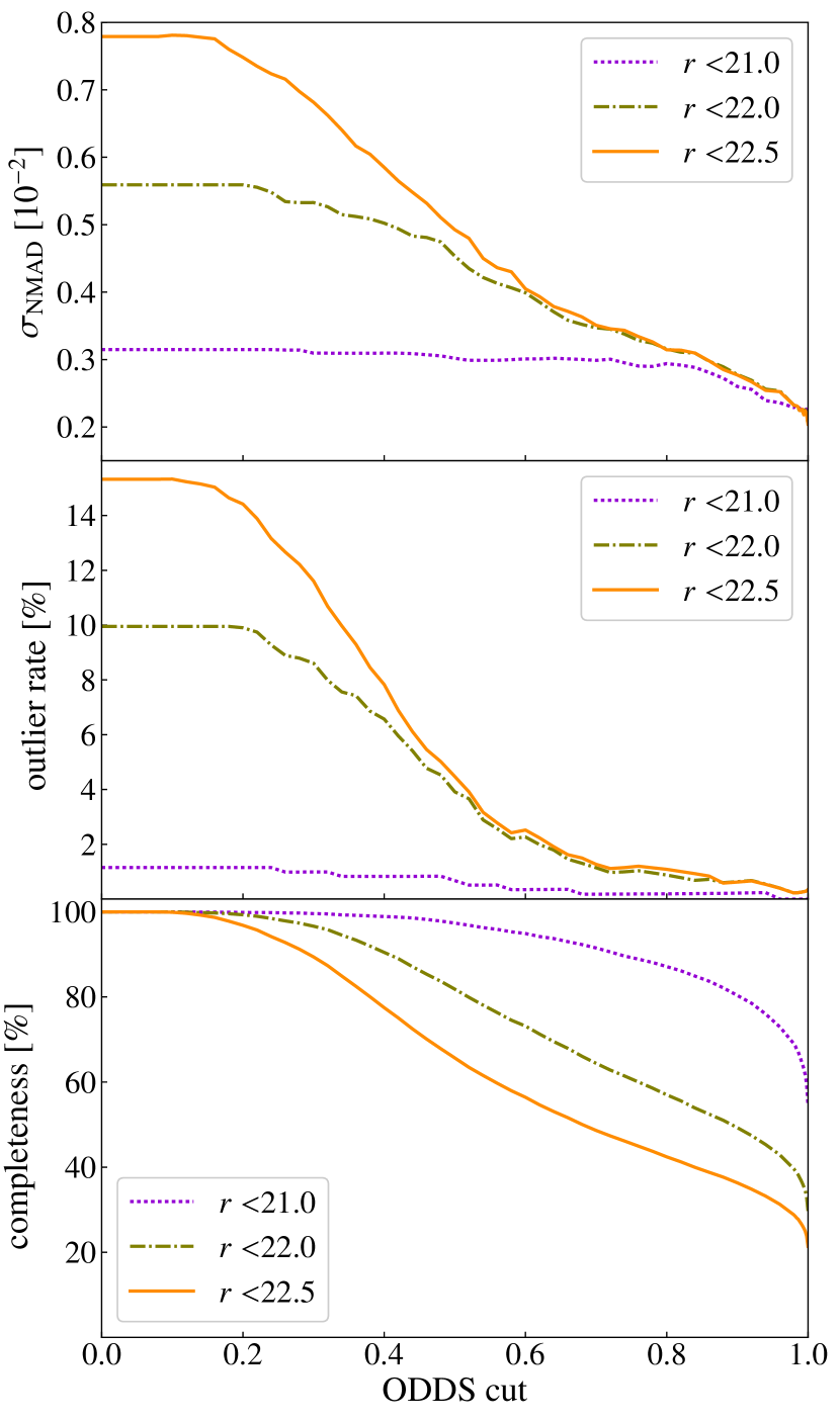
Figure 11: Dependence of the Normalized median absolute deviation of photo-$z$ errors (top panel) outlier rate (middle panel) and completeness (bottom panel) on the ODDS parameter for different $r$-band cuts.

The accuracy of the photo-$z$ for galaxies also depends on their spectral class. In particular, LRGs are expected to have more accurate photo-$z$ compared to the general population at the same magnitude thanks to a strong 4000 Å spectral break. To estimate the photo-$z$ accuracy for LRGs we split miniJPAS galaxies in two samples according to the starforming/quiescent classification based on SED-fitting, discussed in Sect. 6.2.3, which has been performed for galaxies with $r<22.5$. This classification is broadly consistent with a red/blue classification based on the Dn(4000) index, which measures the strength of the $4000$ Å  break (see Balogh et al. 1999). Figure 12 shows the redshift accuracy as a function of the limiting magnitude for the subsamples of passively evolving and main sequence/star-forming galaxies. Note that the redshift precision of blue galaxies depends more strongly with magnitude. This is because at fainter magnitude the emission lines typical of star-forming galaxies become weaker and we have to rely on the continuum to estimate the photo-$z$. For passive galaxies, instead, the precision of the photo-$z$ estimate decreases only weakly with magnitude. This same classification and the results on redshift accuracy are used in Sect. 6.3 to discuss the derived number densities of red and blue galaxies, in view of clustering studies of the large scale structure.

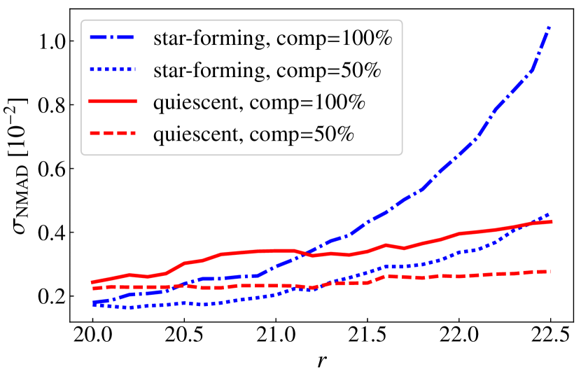
Figure 12: Dependence of photo-$z$ errors on the limiting magnitude in the $r$-band for galaxies in the “passive” subsample (red line) compared to other galaxies (main sequence and starburst galaxies, blue line). Solid lines indicate values for 100% completeness (no cut in ODDS) while dashed lines correspond to the 50% with highest ODDS in each magnitude bin.

4.2.3 Extinction and cross-matches

We provide an estimation of the integrated $E(B-V)$ colour excess due to the Milky Way extinction along the line of sight of each detected source in the database table minijpas.MWExtinction. This was derived from the Bayestar17 (Green et al. 2018b) dust maps and coupled with the extinction coefficients $k_{\lambda}$ gathered in table minijpas.Filter and computed from the Schlafly et al. (2016) extinction curve following the prescription in Whitten et al. (2019b). In addition to the $E(B-V)$ value, we also provide a precomputed extinction correction $k_{\lambda}\,E(B-V)$ for each source.

Finally, we provide the cross-match with the surveys listed in Table 9. For catalogues with a Vizier ID, the cross-match has been performed using the CDS X-Match Service. We warn the reader that we report, for each miniJPAS source, all the objects within the search radius. Therefore, a miniJPAS source may have multiple counterparts in the cross-match catalogues.

Table 9: List of external catalogues for which a precomputed cross-match with miniJPAS is provided.

Catalogue Name	Reference	Vizier ID	Search radius	Data base table
J-PLUS DR1	Cenarro et al. (2019)	—	3”	xmatch_jplus_dr1
ALHAMBRA Survey	Molino et al. (2014)	J/MNRAS/441/2891/photom	4”	xmatch_alhambra
Gaia DR2	Gaia Collaboration et al. (2018)	I/345/gaia2	1.5”	xmatch_gaia_dr2
PanSTARRS DR1	Chambers et al. (2016)	II/349/ps1	1.5”	xmatch_panstarrs_dr1
SDSS DR12	Alam et al. (2015)	V/147/sdss12	1.5”	xmatch_sdss_dr12
All WISE	Cutri & et al. (2014)	II/328/allwise	4”	xmatch_allwise
GALEX AIS	Bianchi et al. (2011)	II/312/ais	4”	xmatch_galex_ais
CFRS	Lilly et al. (1995)	VII/225B/catalog	4”	xmatch_cfrs
DEEP2	Coil et al. (2004)	II/301/catalog	1.5”	xmatch_deep2_photo
DEEP2 All	Matthews et al. (2013)	III/268/deep2all	1.5”	xmatch_deep2_spec
HSC-SSP PDR2	Aihara et al. (2019)	–	1.5”	xmatch_subaru_pdr2

4.3 Data access

Large projects like J-PAS require an easy and agile access to the data. For this purpose, CEFCA has developed a powerful Science Web Portal offering advanced tools for data search, visualization and download, each suited to a particular need (Civera & Hernandez 2020). The data of this Public Data Release (PDR-201912) of miniJPAS can be accessed here: http://archive.cefca.es/catalogues/minijpas-pdr201912.

The portal includes a user-friendly sky navigator service including colour images of the survey. Sources are highlighted, and clicking on an object allows the user to visualize a summary of its properties and J-spectra. Further object exploration is possible through an Object Visualization tool. This tool displays the detailed information about the selected source and the image thumbnail in each filter. It also provides tools to download reports and custom object fits cutouts and to perform cross matches with other catalogues.

An object list search tool is also offered, which lets the user upload a list of sky positions, object names or object identifiers and then returns a list of objects near those positions, displaying a customizable summary, J-spectra and thumbnail images for all of them. Users can also retrieve a list of objects within a certain angular distance to a given sky position, fulfilling additional brightness and photometric redshift criteria if needed, using the cone search service.

To download the full coadded images and derived products, an image search service has been implemented where users can select and download the desired data using a variety of search criteria. A coverage map service is also available which helps users to visualise the sky area covered and the distribution of the pointings of the survey. With the Multi-Order Coverage maps (MOC) download service (Fernique et al. 2019), users can download the MOC file which describes the area covered by the survey and can be used to compute very fast data set operations (e.g., unions, intersections) or query data (e.g., sources, images) of other data releases only inside this data release area, using external tools like VizieR, Aladin or Topcat.

An asynchronous queries interface based on Virtual Observatory (VO) Table Access Protocol (TAP, Dowler et al. 2010) has also been implemented in the portal where users can perform Astronomical Data Query Language (ADQL) queries (Osuna et al. 2008) directly to the database. All of these services support the Simple Application Messaging Protocol (SAMP Boch et al. 2012) that enables the catalogues portal to interoperate and communicate with VO-compatible applications .

Catalogue data and images are also accessible through VO protocols (Hernandez & Civera 2020). These VO services allow the users to access data in a standardized way using VO compatible applications or their own scripts. Images are available via the Simple Image Access Protocol (SIAP, Dowler et al. 2015) that allows not only to search for all images covering a sky region, but also to retrieve the full fits images, cutouts or colour images. Catalogue data is accessible both via Simple Cone Search (SCS, Plante et al. 2008) and TAP. The first allows to search all the objects within a given radius around a specified location, while TAP offers a more flexible access to data tables allowing perform complex searches (using ADQL) on the tables storing information of images, filters, objects and photo-$z$.

Below we provide a summary of the different tools available to access the data:

Sky Navigator. Sky exploration by panning and zooming. By clicking on an object, one obtains a summary of its properties and the options to explore it or search it in other catalogues.

Object List Search. Search for a list of objects via sky positions, object names or objects identifiers. It returns a list of sources near those positions and displays a summary, photo-spectra and thumbnail images for the list of objects.

Image search. Search and download images by position or name.

Cone search. Search the database for objects near a certain sky position. Restrictions on colors, magnitudes and photo-$z$ can be added.

Coverage map. Shows the sky area covered by the data release. The map is linked to the Sky Navigator.

Multi-Order Coverage Map (MOC). To download the Multi-Order Coverage map (MOC), which describes the area covered by the data release (FITS file).

VO Services. Access to images and objects data through the Virtual Observatory (VO) protocols using VO compatible applications. VO services offered are Simple Cone Search (SCS), Table Access Protocol (TAP) and Simple Image Access Protocol (SIAP).

VO Asynchronous Queries (ADQL). Search the database via Astronomical Data Query Language (ADQL) queries. A help manual with examples is provided.

Direct Download Services. Allow easy automatic access to most of the data. It is possible to download directly some data through simple HTTP access. The data currently available through this service include:

• Full images and weight maps in FITS format and PNG.

• “On-demand” cutouts of images and weight maps in FITS and PNG formats.

• Masks of individual images in MANGLE format.

• PSF models of full frames in PSFEx format or as actual FITS images of PSF models in a given position of any image.

• “On-demand” PSF models for a given position and image in FITS format.

• photo-$z$ catalogues.

• Information on the original individual images.

5 Data quality

In this section we show the results of a variety of tests aimed at characterizing the quality of the data.

5.1 Homogeneity across the footprint

A powerful test of the consistency of the data reduction and photometric calibration is the comparison of the photometry of objects in the overlap area of adjacent pointings. For these objects the data reduction and calibration have been performed twice, in an independent way in each pointing (see Sect.  3.5). Based on the miniJPAS observation strategy, the overlap area is approximately 10% of the whole area of the total footprint (see Sect. 2.4.1).

We have compared the magnitudes of point sources (CLASS_STAR $>0.5$) within a 6 arcsec aperture, taking into account the corrections to the flux driven by the variations of the PSF between the different observations (i.e., the light profile of the point sources was used to extend the flux beyond the cut-off at 6 arcsec). The result of that comparison is shown in Fig. 13 for the $r$ band, where we plot the difference in the magnitudes for each object in the overalap area of two contiguous tiles, $\Delta r=r_{a}-r_{b}$, as a function of the mean magnitude, $r=(r_{a}+r_{b})/2$, with error bars given by $\sigma=(\sigma_{a}^{2}+\sigma_{b}^{2})^{1/2}$, where $a,b=$ 1, 2, 3, 4 (the four miniJPAS pointings). In the figure we show the differences in magnitudes before (light symbols) and after (heavy symbols) the PSF correction. From the scatter of the data points we can estimate the calibration error for each filter: in the case of the $r$ band, this additional uncertainty due to the photometric calibration should be of the order of $\sigma_{\rm zpt}\simeq 0.005$ in order to obtain a reduced $\chi^{2}$ of 1. However, this calibration error is different for each filter, with the upper limit being set by the filters in the blue-end of the spectrum. These show  a calibration error of approximately $0.04$ magnitudes (see Sect. 3.5). We stress, however, that the current statistics is too small to properly use this procedure to estimate calibration errors. This will not be a problem for J-PAS, where areas observed will be three order of magnitude larger, and the strategy will include a larger overlap area.

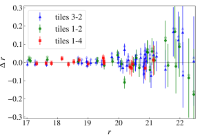
Figure 13: Magnitude differences in objects in overlapping tiles for the $r$ band (rSDSS), using a fixed aperture of 6 arcsec. Each point corresponds to a point source in one of the overlapping areas (distinguished here by colors). The light symbols are the magnitude differences before correcting for the PSF of each tile, and the heavy symbols are the magnitude differences after that correction is applied. The error bars are those of the individual tiles, added in quadrature.

5.2 Comparison with other surveys

We further test the quality of the data by comparing our photometry with that from other surveys. The broad band photometry is compared with that from SDSS and HSC-SSP, while the narrow band photometry is compared with synthetic photometry derived by convolving SDSS spectra with the J-PAS filters, as detailed below:

Broad band photometry

We compare the broad band photometry of miniJPAS with the one of SDSS and HSC-SSP. We use sources with no warnings or flags and the MAG_AUTO photometry, which is a proxy of total magnitude. For this comparison we use colors, as they best reflect the SED of the sources. Colours are also very useful to check the quality of the relative calibration in miniJPAS. We show in Fig.  14 the $(r-i)$ color difference of miniJPAS and SDSS/HSC-SSP, as a function of the miniJPAS $r$-band for both point-like and extended sources, where point sources are defined to be the ones with CLASS_STAR ¿ 0.9. We immediately see that colors in miniJPAS with respect to SDSS and HSC-SSP are generally consistent. The lack of systematic shifts in the comparison with SDSS confirms the quality of the calibration. As expected, the scatter is larger in the comparison with SDSS than in the one with HSC-SSP, because of the shallower depths reached by SDSS. We get similar results when comparing the colors from other broad bands. The good agreement for both point and extended sources confirms not only the quality of the calibration, but also that we can trust the SED of galaxies for extragalactic studies.

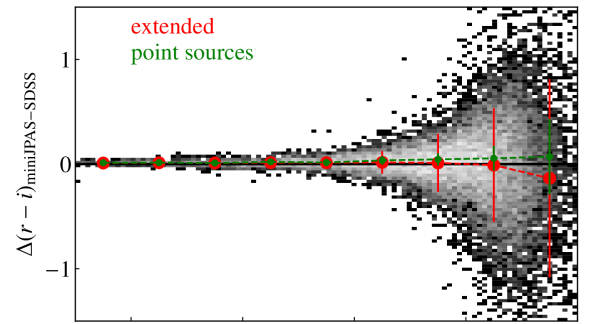
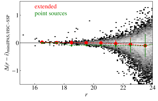
Figure 14: Color $(r-i)$ difference of miniJPAS and SDSS (upper panel) and HSC-SSP (lower panel) as a function of the miniJPAS $r$ band. The gray density map is for all objects. The coloured points indicate the median with 1-$\sigma$ error in different magnitude bins for extended (red) and point sources (green).

Narrow band photometry

We compare the narrow-band photometry of miniJPAS with the synthetic photometry obtained by convolving SDSS spectra with the transmission curves of the J-PAS filters. We use the spectra available in the SDSS DR12 of galaxies with magnitude in the miniJPAS $r$-band $r\leq 20$ and $20\leq r\leq 22.5$ in the MAG_PSFCOR photometry. We used the MAG_PSFCOR photometry to avoid aperture corrections. In any case, we scaled the spectra (in AB magnitudes) to the median of the $g,r,i$ miniJPAS MAG_PSFCOR photometry to account for the differences in aperture between the SDSS fibre and the miniJPAS photometry. In total, there are 405 spectra at $r\leq 22.5$, of which 122 at $r\leq 20$. Figure 15 shows the mean of the difference between the observed and the synthetic magnitudes for each narrow band filter. The mean of the shifts is $0.006\pm 0.028$ and the median scatter is $0.06$. These small values confirm the accuracy of the miniJPAS narrow-band calibration. The scatter is larger for galaxies with 20 $\leq r\leq$ 22.5 than for brighter objects due to the shallower depth reached by SDSS, and it is larger in the blue than the red narrow-band filters.

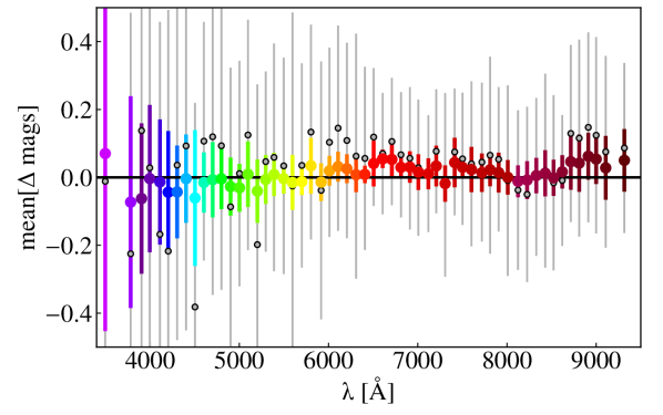
Figure 15: Difference between miniJPAS photometry (MAG_PSFCOR magnitudes) and synthetic photometry derived by convolving SDSS spectra with the J-PAS filters. Coloured symbols, and thick error bars, correspond to galaxies with $r<20$, while gray circles with thin error bars to galaxies with $20<r<22.5$. The error bars refer to the scatter of the distribution within each filter.

5.3 miniJPAS completeness

The definition of the limiting flux at which a survey is not biased in detection, a.k.a. completeness, is one of the key points that must be addressed during the preliminary analysis and data validation phase. The J-PAS survey will include an automatic pipeline devoted to determining the completeness curves of the composite images or tiles. Here, we first briefly introduce the methodology and completeness curves obtained for miniJPAS, which will then be confronted with the results obtained from the comparison with HSC-SSP.

Our pipeline is based on the use of synthetic images of galaxies and stars, which are treated separately. The completeness of each pointing is obtained after injecting in random positions without previous detections a position-dependent PSFs for point-like sources and light profiles of galaxies extracted from COSMOS HST images in the $F814W$ for extended sources. In the latter case, an average colour term is applied to transport the structure measured in $F814W$ to the appropriate scale in the miniJPAS filters, and the original profile is convolved with the corresponding position-dependent PSF. The completeness curves are then calculated from the fraction of injected sources that the source detection process recovers (see Sect. 3.4). We note that this analysis must be made for each of the miniJPAS pointings to account for discrepancies related, for example, to different observational conditions. In Fig. 16 we show the derived completeness curves, both for compact and extended sources. The curves are properly fitted by a Fermi-Dirac distribution function (see e.g. Sandage et al. 1979; Díaz-García et al. 2019) of the form:

$$\mathcal{C}=\frac{100}{\exp{\left\{(r_{\mathrm{JPAS}}-\mathcal{C}_{50})/\Delta_{\mathcal{C}}\right\}}+1},\$$ (1)

where $\mathcal{C}$ is the detection fraction (in per cent units), $\mathcal{C}_{50}$ is the magnitude at which the sample is $50$% complete, and $\Delta_{\mathcal{C}}$ the decay rate on the fraction of detections. In Table 10, we show the parameters that result from fitting Eq. (1) to miniJPAS data. We estimate that the sample of point-like sources in the full miniJPAS catalogue is $99$% complete up to $r\sim 23.6$ (MAG_AUTO). For extended sources this limit is constrained at $r\sim 22.7$. It is worth mentioning that the miniJPAS-AEGIS1 field is deeper than the other pointings with limiting fluxes at $r\sim 24.1$ and $r\sim 23.3$ for point-like and extended sources, respectively.

With a typical seeing of $0.6-0.8$ arcsec in the optical range, along with a depth of $r\sim 26$ ($5$ $\sigma$ limit within a $2$ arcsec diameter aperture), the HSC-SSP survey can be used to test the miniJPAS completeness. To carry out the comparison, we used the second data release of the HSC-SSP survey (Aihara et al. 2019) as the reference catalogue for the HSC-SSP photometry. The overlap area with miniJPAS is of $0.7$ deg². Taking as reference the $r$ band from HSC-SSP (cmodel magnitudes, which are a proxy to total magnitudes), we computed the fraction of common detections between HSC-SSP and miniJPAS at different magnitude ranges, following a similar procedure than the one described above for the injection of synthetic images. Owing to the lower seeing of the HSC-SSP observations, we used as compactness discriminator the parameter r_extendedness_value provided by the HSC-SSP catalogues. To perform a robust and fair determination of the completeness, we quadratically include the systematic uncertainties reported by Huang et al. (2018) for both PSF and cmodel magnitudes (see Tables 1 and 3 in Huang et al. 2018). The impact of these uncertainties on the fraction of common detections is determined via a Monte Carlo approach by assuming Gaussian errors for the $r_{\mathrm{HSC}}$ fluxes. Nevertheless, discrepancies between the HSC-SSP and the miniJPAS observations (e.g. seeing, deblending, etc.) may yield systematic discrepancies in the fraction of common sources, typically ranging from $5$ to $10$%, even when both surveys are not biased by incompleteness. To account for this effect and obtain alternative completeness curves based on HSC-SSP data, we fitted the fraction of common detections to Eq. (1), adding a linear term of the form $\alpha\cdot r_{\mathrm{HSC}}+\beta$ (with $\alpha$ and $\beta$ as free parameters). Figure 16 illustrates the fraction of common detected sources in the HSC-SSP and the miniJPAS surveys for extended and point-like sources, as well as the fits following Eq. (1), with and without the added linear term. We find a good agreement between the completeness curves obtained from synthetic sources and from the comparison with HSC-SSP observations, within a 1$\sigma$ uncertainty level (see also Table 10). In addition, there is no discrepancy between the detection of common point-like sources, and therefore, $\alpha$ and $\beta$ are fully compatible with a null value. Regarding the miniJPAS-AEGIS3 pointing, we are not able to observationally determine the completeness curve of point-like sources owing to the very low overlapping area. For extended sources, there exist systematic discrepancies at $r_{\mathrm{HSC}}\gtrsim 20$ in all the miniJPAS pointings, which were properly taken into account by the linear term added to Eq. (1).

We note that the completeness curves were obtained from total (synthetic) magnitudes in miniJPAS and from cmodel magnitudes in HSC-SSP. Regarding the practical application of the completeness curves, the AUTO magnitude is our best proxy for a total magnitude and should be used as reference to define a complete flux-limited sample. Consequently, the limiting magnitudes in all the fields of miniJPAS for the dual mode catalogues are $r_{\texttt{AUTO}}=23.6$ and $22.7$ for point-like and extended sources, respectively. The completeness curve parameters are available in the ADQL table minijpas.TileImage.

Table 10: Parameters describing the completeness function of the mini-JPAS survey obtained from injection of synthetic sources ($\mathcal{C}_{50}$ and $\Delta_{\mathcal{C}}$, see Eq. (1) ) and after comparing with the fraction of common sources with respect to HSC-SSP photometry catalogues ($\mathcal{C}_{50}^{\mathrm{HSC}}$ and $\Delta_{\mathcal{C}}^{\mathrm{HSC}}$). In the last column, we present the limiting values for a completeness level of $99$% for the miniJPAS detection band ($r$, MAG_AUTO).

Field	$\mathcal{C}_{50}$	$\Delta_{\mathcal{C}}$	$\mathcal{C}_{50}^{\mathrm{HSC}}$	$\Delta_{\mathcal{C}}^{\mathrm{HSC}}$	$r_{\mathrm{99}}^{\mathrm{AUTO}}$
Point-like
miniJPAS-AEGIS1	$24.74$	$0.14$	$24.57^{+0.09}_{-0.09}$	$0.13^{+0.06}_{-0.06}$	$24.10$
miniJPAS-AEGIS2	$24.33$	$0.16$	$24.33^{+0.16}_{-0.12}$	$0.23^{+0.11}_{-0.08}$	$23.59$
miniJPAS-AEGIS3	$24.39$	$0.16$	–	–	$23.65$
miniJPAS-AEGIS4	$24.26$	$0.14$	$24.26^{+0.12}_{-0.10}$	$0.20^{+0.08}_{-0.07}$	$23.62$
Extended
miniJPAS-AEGIS1	$24.22$	$0.21$	$24.39^{+0.07}_{-0.08}$	$0.29^{+0.09}_{-0.06}$	$23.26$
miniJPAS-AEGIS2	$23.86$	$0.24$	$24.03^{+0.07}_{-0.07}$	$0.33^{+0.04}_{-0.03}$	$22.76$
miniJPAS-AEGIS3	$23.88$	$0.26$	$24.11^{+0.14}_{-0.15}$	$0.39^{+0.09}_{-0.07}$	$22.69$
miniJPAS-AEGIS4	$23.89$	$0.22$	$24.09^{+0.07}_{-0.07}$	$0.34^{+0.04}_{-0.04}$	$22.88$

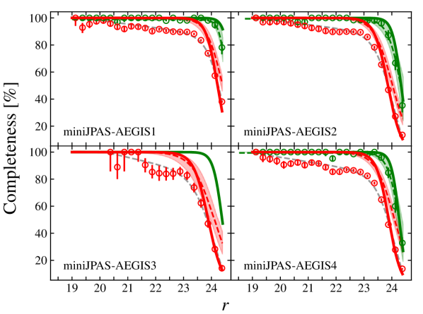
Figure 16: Completeness of extended and point-like miniJPAS sources as a function of total magnitude in the miniJPAS $r$ band for the four miniJPAS pointings. The solid lines are the completeness curves of extended and point-like sources (red and green, respectively) obtained from a synthetic injection of sources. The red (green) circles illustrate the observed fraction of common extended (point-like) sources in the miniJPAS and HSC-SSP surveys (this comparison is not possible for miniJPAS-AEGIS3, given the small overlap between this pointing and HSC-SSP). The dashed coloured lines are the completeness curves obtained from the comparison with the HSC-SSP dataset, with uncertainties highlighted by the shaded area (see the text for the description of their derivation). The dashed gray lines show the curve that best fits the fraction of common sources (Eq. 1 plus a linear term, details in text).

5.4 Number counts

We present the stellar and galaxy number counts in Fig. 17. To derive the number counts separately for point-like and extended sources we used the stellar-galaxy locus classification presented in Sect. 4.2.1, corrected for the completeness derived by synthetic images as described above. The number counts derived from the Bayesian classification agree with the expectations from the literature both for stars and galaxies up to $r=23.5$, as shown in Fig.  17. The derived probabilities are publicly available in the ADQL table minijpas.StarGalClass.

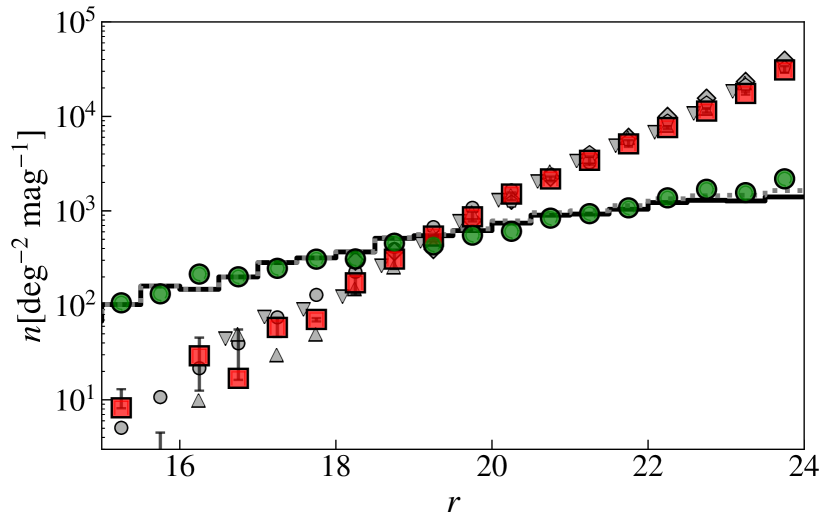
Figure 17: Stellar (green circles) and galaxy (red squares) number counts as a function of the $r$ band magnitude. The black solid curve is the stellar number counts at the EGS position estimated with the default TRILEGAL model of the Milky Way (Girardi et al. 2005). The dotted gray curve includes the expected contribution for point-like quasars (from the BOSS survey, Palanque-Delabrouille et al. 2016) to the compact population. Gray symbols are galaxy number counts from the literature: Yasuda et al. (2001, circles); Huang et al. (2001, triangles); Kümmel & Wagner (2001, inverted triangles); Kashikawa et al. (2004, diamonds); and Capak et al. (2004, pentagons).

5.5 Caveats and known problems

We provide below a brief list of issues and caveats to keep in mind when using the data-release presented in this paper:

Inhomogeneous exposure times.

Narrow bands present heterogeneous total exposure times from band to band and from pointing to pointing as, in some cases, more than the planned number of images was used to produce the co-adds. For JPCam observations the strategy will be defined to obtain more homogeneous depths.

Extended faint sources.

The superbackground subtraction described in Appendix B, together with the small dithering pattern of miniJPAS, makes extended sources to be potentially confused with instrumental background. Therefore, for miniJPAS data we cannot discard that some faint extended real sources have been totally or partially removed from the final images. For J-PAS data, this issue is not expected because of its high dithering pattern of 1/2 CCD.

Image quality.

Since the time window to complete the miniJPAS project was limited, the initial requirements in terms of seeing, airmass and atmospheric stability were at times relaxed to guarantee the completion of the whole project on time. This has led to PSFs which are on average larger than what the system can typically provide (¡1 arcsec), and to the presence of some thin clouds for the latest tray of reddest filters (mainly in J0790 filter and redder), which were detected only after the data reduction.

Fringing correction.

The time limitation in the observations of miniJPAS resulted in a number of scientific images which turned out to be scarce to generate high-quality, master fringing images for all red filters. This means that the final fringing removal is not optimal in all cases.

Astrometric accuracy in coadded images.

Despite single individual images exhibit astrometric solution accuracies with respect to Gaia DR2 of the order of $\sim 0.03$ arcsec , these degrade to up to $\sim 0.3$ arcsec in the case of coadded images and dual-mode catalogues. Resampling and pixel rotations before coadding seems to be the main source of this effect, which will certainly be revisited in future releases.

6 A foretaste of J-PAS science

In this section we give a brief overview of the wide variety of scientific cases that can be addressed thanks to the J-PAS filter system. We use miniJPAS data to provide concrete examples and we discuss results in view of the upcoming J-PAS data. Representative J-spectra of the wide variety of astrophysical objects in the surveyed area are presented in 18.

6.1 Galactic Science

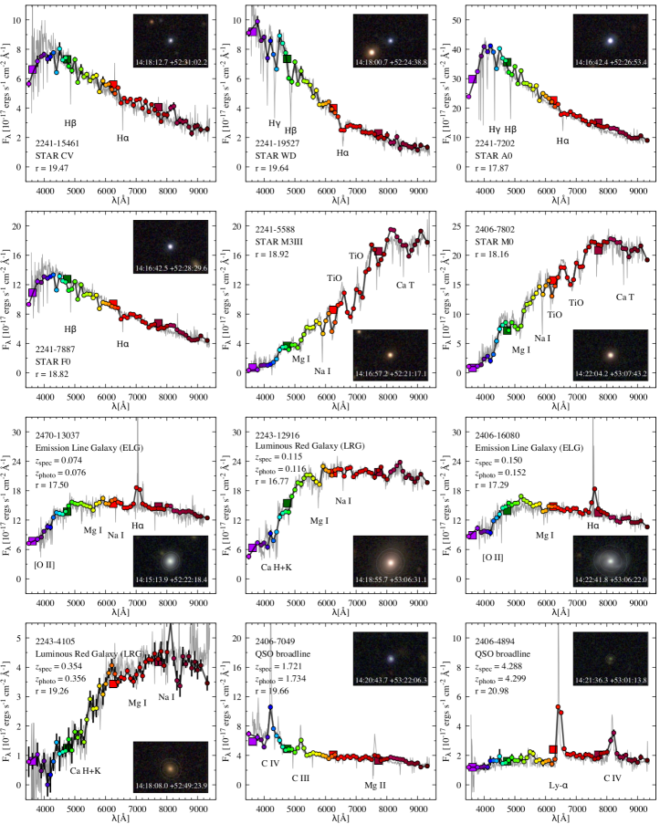
Figure 18: The J-spectra of different classes of stars, galaxies and quasars in the miniJPAS field (coloured symbols) compared with the SDSS spectra (gray lines). The miniJPAS object ID, $r$ magnitude, and classification are listed in the legend. Extragalactic sources are ordered by increasing redshift, and both spectroscopic (SDSS) and photometric (miniJPAS) redshift are provided in the legend. The multi-color inset images are centred on the object and are $30$ arcsec across. The ellipses visible for extended sources are the ¡auto ellipse¿ (inner ellipses) and the ¡petro ellipse¿ (outer ellipses).

The unique J-PAS photometric system is able to provide the equivalent of a low-resolution spectrum for each stellar source within its footprint. Key absorption features, as well as the shape of the SED, can be used to identify, classify and characterize targets of interest. In addition, the J-spectra allow for the determination of stellar atmospheric parameters (effective temperature, surface gravity, and metallicity) and selected chemical abundances. Basic approaches used to derive stellar parameters can be based on photometry (Ivezić et al. 2008; An et al. 2015; Starkenburg et al. 2017; Huang et al. 2019), the fitting of theoretical SED’s (Allende Prieto 2016), or on the application of machine learning algorithms (Li et al. 2018; Thomas et al. 2019; Whitten et al. 2019b). Previous experience with the Stellar Photometric Index Network Explorer (SPHINX, Whitten et al. 2019b), applied to the Early Data Release of J-PLUS (Cenarro et al. 2019) has shown the reliability of estimating effective temperature and metallicity based on narrow-band photometry, achieving $\sigma(T_{\rm eff})=91$ K and $\sigma([\rm{Fe}/\rm{H}])\sim 0.2$ dex. A key ingredient for a successful application of any machine learning technique is the definition of an adequate training dataset, which should ideally sample a parameter space as complete as possible. Examples of large medium-resolution spectroscopic databases in the northern hemisphere that can help address this issue are the SEGUE (Sloan Extension for Galactic Understanding and Evolution; Lee et al. 2008), LAMOST (Large Sky Area Multi-Object Fiber Spectroscopic Telescope; Li et al. 2018, Boeche et al. 2018), and APOGEE (Apache Point Observatory Galactic Evolution Experiment; Majewski et al. 2017).

Different topics in stellar astrophysics can be addressed once the stellar parameters have been estimated. A few science cases include the search for metal-poor stars (Youakim et al. 2017; Yoon et al. 2018; Placco et al. 2018, 2019), blue horizontal branch stars (Santucci et al. 2015b; Whitten et al. 2019a; Starkenburg et al. 2019), blue stragglers (Santucci et al. 2015a), ultracool dwarfs, and white dwarfs. Other topics include the identification and chemical characterization of Galactic stellar streams, classical dwarf galaxies and ultra-faint dwarf galaxies (e.g., Longeard et al. 2018; Shipp et al. 2018, 2019; Chiti et al. 2020; Longeard et al. 2020). Systems such as planetary nebulae and symbiotic stars, that involve circumstellar ionized gas, can be also identified and characterized based on the J-spectra  (Gutiérrez-Soto et al. 2020). J-PAS photometry can also contribute to the study of stellar populations of Globular Clusters as shown by Bonatto et al. (2019) for the GC M15, based on J-PLUS Science Verification Data. The PRISTINE survey (Starkenburg et al. 2017) has been successful in determining stellar atmospheric parameters and selecting metal-poor stars by combining SDSS photometry with a narrow-band filter centred on metallicity-sensitive Ca H&K absorption features (3900-4000Å). Since J-PAS has other filters in metallicity-sensitive regions besides the Ca H&K lines, it is expected that the errors and identification thresholds will improve considerably. In addition, J-PAS can provide a powerful data-set to pre-select interesting stellar sources for large-scale wide-field spectroscopic efforts such as DESI (DESI Collaboration et al. 2016) and WEAVE (Dalton et al. 2012).

Examples of stellar sources observed in miniJPAS are presented in the top 6 panels of Fig. 18. The measured fluxes in the narrow filters are shown and compared with the SDSS spectra. The classes and spectral types listed in each panel were retrieved from the SDSS spectroscopic pipeline database. The inset color images have $30$ arcsec across and are centred on the stars. It is possible to see that the miniJPAS photometry is capable of successfully capturing the continuum shape for these stellar sources and also the main spectral absorption features used to determine spectral types, atmospheric parameters, and selected chemical abundances (e.g., carbon, $\alpha$-elements). For the warmer stars (first four panels), the hydrogen Balmer lines are clearly traceable for $\lambdaup<5000$ Å, while for cooler stars (middle and right panels in the second row), several TiO molecular bands are present for $\lambdaup>6000$ Å. The small footprint of miniJPAS does not allow the application of the aforementioned techniques that are currently being applied to the J-PLUS data (Whitten et al. 2019b; Bonatto et al. 2019), as they require large training samples. This will be possible with the much larger areas scanned by J-PAS.

6.2 Galaxy evolution studies

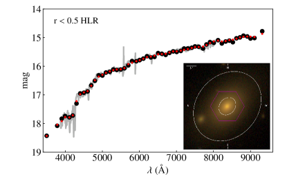
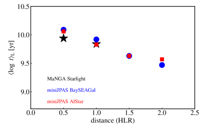
Figure 19: Upper panel: The MaNGA spectrum of the central ring of 0.5 HLR (grey line) of a galaxy at $z\sim 0.1$ is compared with miniJPAS data (black dots). The result of the fitting of miniJPAS data is also plotted (red dots). The inset shows an image of the galaxy in the $r$ band where two ellipses are overlaid at 0.5 HLR and 2 HLR. The FoV of the MaNGA survey is over-plotted as a red hexagon. Bottom panel: Comparison of the radial variation of the average age $\langle\log t\rangle_{L}$ derived from miniJPAS data, with the non-parametric code AlStar (red dots) and the parametric code BaySEAGal (blue dots), and from the MaNGA data analysed with the STARLIGHT code (black stars).

The uniform and un-biased observations of J-PAS will offer a unique large dataset for galaxy evolution studies, from the IFU-like analysis of nearby sources, to stellar population studies across cosmic time. The narrow bands will allow for the detection of strong line emitters, from star-bursting galaxies to quasars. The wide area will also enable the detection of rare objects as well as the study of galaxies in all kinds of environments.

Examples of J-spectra of extragalactic sources observed by miniJPAS are provided in the bottom six panels of Fig. 18. Ordered by increasing redshift, the first four panels show examples of both passive and star forming galaxies. Clearly visible are the $4000$ Å break of red galaxies and the $\rm{H}\alpha$ emission of blue star forming objects. The last two panels, instead, show examples of quasars, with the profiles of broad emission lines, such as Ly$\alpha$, CIV, CIII, clearly traced by multiple filters.

In what follows we provide few examples of galaxy studies based on the miniJPAS dataset.

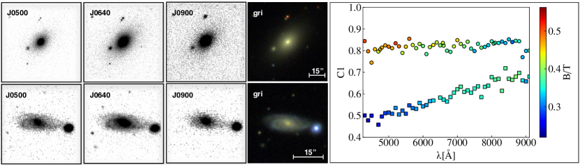
Figure 20: Left panel: snapshots of an elliptical galaxy, ID 2470-10239 (upper row) and a spiral galaxy, ID 2470-10291 (bottom row), in three of the J-PAS narrow bands (J0430, J0640, J0900), as an example of the variation of galaxies’ properties with wavelength. Middle panel: $g,r,i$ broad band colour images of the two galaxies. The $15$ arcsec length, indicated on the images for reference, corresponds to $21.5$ kpc for the elliptical galaxy ($z\simeq 0.075$) and $20.8$ kpc for the spiral galaxy ($z\simeq 0.073$). Right panel: variation of the concentration $C1$ parameter with wavelength, colour coded according to the bulge-to-total light ratio ($B/T$), for the early type galaxy (circles) and the spiral galaxy (squares). The magnitudes are integrated up to 1 disk scale lengths.

6.2.1 J-PAS: a low spectral resolution IFU survey

The combination of the wide area and the CCD pixel size will make J-PAS a competitive IFU-like survey of extended galaxies at $z<0.15$, where the low spectral resolution will be compensated by the large statistics that the survey will provide. In this sense, J-PAS will be highly complementary to CALIFA (Sánchez et al. 2012; García-Benito et al. 2015; Sánchez et al. 2016) and MaNGA (Bundy et al. 2015; Law et al. 2015), by providing larger samples and having the ability of studying galaxy properties to larger galactocentric distances, up to several half-light-radii (HLR), with a significantly better spatial sampling ($0.23$ arsec pixel^-1 for the broad bands and $0.46$ arsec pixel^-1 for the narrow bands). For example, even at $z\sim 0.1$, where the spatial scale is $\sim 1.8$ kpc arcsec^-1, galaxies with a typical HLR of $4$ kpc can be studied every $\sim$0.5 HLR, assuming an average seeing of $1$ arcsec.

Moreover, J-PAS data will not suffer from FoV restrictions, so the spatial properties of the largest galaxies of the Local Volume (distance $\leq 15$ Mpc) will be easily studied.

In the small miniJPAS footprint there are few extended galaxies with a HLR exceeding $5$ arcsec that can be useful to show the potential of J-PAS on this subject. We have chosen, as example, a quiescent galaxy at $z\sim 0.1$ with $14.7$ mag in the $r$ band. This galaxy ($\alpha$ = 14:15:20.37; $\delta$ = 52:20:45.19) was also observed by the MaNGA survey (Bundy et al. 2015), so that we can directly show how results based on the analysis of our J-spectra compare with the results from spectroscopic data. MaNGA data were retrieved from the SDSS DR14 (Abolfathi et al. 2018), and the spectra were analysed using the PyCASSO pipeline (de Amorim et al. 2017). From the miniJPAS data we define the nucleus as the maximum of the galaxy emission at the wavelength 5600 Å, and we estimate the HLR to be 9.4 arcsec. The top panel of Fig. 19 shows a comparison between the MANGA spectra and the miniJPAS photometric data within $0.5$ HLR, demonstrating the very good agreement in terms of flux and SED. We derive the spatially-resolved stellar population properties of the galaxy by analysing both miniJPAS and MaNGA data in rings centred on the nucleus. While the MaNGA FoV allows to study the galaxy properties in the first two rings (within $1$ HLR, see the inset in Fig. 19), with miniJPAS data we can extend the analysis up to $2$ HLR. The miniJPAS J-spectra of the 4 rings are fitted by BaySEAGal (de Amorim et al. in prep), a Bayesian code that allows to derive a wide variety of intrinsic galaxy properties, such as the stellar mass, the luminosity-weighted age of the stellar population, the metallicity and stellar extinction. For comparison, we also fit the J-spectra with the non-parametric code AlStar (Cid Fernandes et al. in prep.). Both codes use the same set of single stellar populations (SSP) models by Bruzual & Charlot (2019, in prep.) to build the star formation histories. The magnitudes obtained from the fitting with BaySEAGal are plotted in Fig. 19. The MaNGA spectra of the two inner rings are instead fitted with the non-parametric code STARLIGHT (Cid Fernandes et al. 2005; López Fernández et al. 2016), and following the same processes used for CALIFA data (de Amorim et al. 2017), using the same set of SSPs. We find a very good agreement in the stellar population properties derived from the parametric and non-parametric codes (AlStar and BaySEAGal) with miniJPAS data, and these results also agree with the ones derived from the MaNGA spectroscopic data. In the bottom panel of Fig. 19 we show, as an example, the results for the radial distribution of luminosity-weighted stellar ages $\langle\log t\rangle_{L}$. Note that this negative age gradient was also found in the CALIFA sample (González Delgado et al. 2015), and in a few extended galaxies in the ALHAMBRA survey (San Roman et al. 2018). The stellar mass in the inner $0.5$ HLR is estimated to be $10^{11.10}\rm{M}_{\odot}$ and $10^{11.06}\rm{M}_{\odot}$ from the MaNGA and miniJPAS analysis, respectively.

J-PAS will also be competitive for IFU-like studies of star forming galaxies of the nearby Universe. The HII regions distributions and their ionized gas properties will be retrieved for galaxies of the Local Volume ($z<0.015$), in similar way as it has been done for J-PLUS (Logroño-García et al. 2019, following the methodology of Vilella-Rojo et al. (2015)). Several methodologies can be developed to retrieve the emission line flux for galaxies out of the Local Volume. One of these is based on a Neural Network method that estimates the equivalent width of the emission lines of H$\alpha$, H$\beta$, [NII]$\lambda$6584, [OIII]$\lambda$5007 using a collection of spectra from the CALIFA and MaNGA surveys used for training (Martínez-Solaeche et al., in prep.).

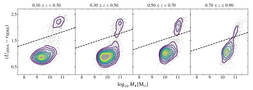
Figure 21: Rest-frame stellar mass-colour diagram corrected for extinction, showing the distribution of star-forming (lower cloud) and quiescent (upper cloud) galaxies at four redshift intervals. The dashed black line illustrates the lower colour limit of quiescent galaxies as a function of stellar mass and redshift. Yellow (purple) contours illustrate higher (lower) densities.

6.2.2 Morphological studies in multi-color

The morphology of galaxies, derived from the analysis of photometric data, can vary with wavelength, as different stellar populations present different colors. For example, if the disk of a galaxy is characterized by a young, star-forming population, while the spheroid is old and metal rich, the Sérsic index will increase for redder wavelengths (Vulcani et al. 2014; Vika et al. 2015). Several works have been already exploring the variation of morphological parameters with wavelengths and recovered the star formation history and stellar population of the different galaxy components. The number of fitted wavelengths has been increasing during the years, from, e.g., the 5 broad bands of the SDSS survey ($ugriz$, Bottrell et al. 2019), to the 9 of the GAMA survey (SDSS + UKIDSS, Kennedy et al. 2016) and the $\simeq 15$ bands in the Dustpedia project (GALEX, SDSS, 2MASS/UKIDSS, WISE, Davies et al. 2017). The J-PAS data set will be unique for this type of studies, as it will provide a low-resolution spectrum for each galaxy component and multicolor CAS (concentration, asymmetry, entropy) parameters. Vika et al. (2013) showed, using SDSS data, that a multi-band bulge-to-disk light decomposition is reliable up to $z\sim 0.3$, while the CAS parameters have been used to define morphological properties up to $z\sim 0.25$ using SDSS data (Ferrari et al. 2015) and even up to $z\sim 3$ using the Hubble Space Telescope GOODS ACS and Hubble Deep Field images (Conselice 2003).

Figure 20, generated with miniJPAS data, gives a taste of the J-PAS potential. From a purely qualitative perspective, the first three panels show how an early- and a late-type galaxy appear at different wavelengths. While the isophotal intensity of the early type galaxy increases with increasing wavelength, since the majority of its mass comprises old and metal rich stars, for the late type galaxy the spiral arms, where most star formation occurs, fade away at red wavelengths. The colors of the different components are also clearly visible in the middle $g,r,i$ color image. More quantitatively, we show in the right panel, for both galaxies, the variation with wavelength of the concentration $C1$, which ranges from 0 to 1. This was derived using the non-parametric code MFMTK (Ferrari et al. 2015). The symbols are color-coded according to the bulge-to-total light ratio, obtained performing a bulge-to-disk light decomposition of the galaxy images using GALFITM, a multi-wavelength extension of GALFIT (Peng et al. 2011). For the early type galaxy the concentration is nearly constant with wavelength, while for the late type galaxy $C1$ increases with increasing wavelength. The spiral galaxy is disk-dominated ($B/T<0.25$), while in the early type galaxy the bulge and the disk contribute almost equally to the galaxy light. Interestingly, while for the spiral galaxy the B/T ratio increases with increasing wavelength, i.e. the percentage of light associated with the bulge is higher in redder bands, in the early type galaxy the bulge is slightly more prominent in bluer bands. Novel techniques, e.g., the Kurvature method of Lucatelli & Ferrari (2019), allow to disentangle the structural multi-components of a galaxy and give indication of the transition regions and allow to infer the presence of other features, such as bars and nuclear disks. All this information, together with the SED fitting of the J-spectra  allow to obtain a full picture of the build-up of galaxy structures (Cortesi et. al. in prep).

In conclusion, the J-PAS filter system will allow to accurately recover galaxy morphologies as well as to study structural and stellar population properties. The wide area of J-PAS will also allow to observe and characterize peculiar and rare objects in all kinds of environment, such as jellyfish galaxies and green peas.

6.2.3 Galaxy properties across cosmic time

The accuracy of the photometric redshifts and the full J-spectra allow to characterize the galaxy population and their properties from the nearby universe up to $z\sim 1$. By fitting the continuum with parametric or non-parametric star formation histories, one can constrain stellar population properties of galaxies, as well as segregate galaxy populations according to their star-formation activity (see, e.g., Cid Fernandes et al. 2005; Mathis et al. 2006; Walcher et al. 2011; Moustakas et al. 2013). The ability of the J-PAS narrow band-filters in extracting physical parameters of galaxies have been studied in Mejía-Narváez et al. (2017) for a variety of star formation histories. The authors used SED fitting codes (TGASPEX and DynBaS Magris C. et al. 2015) to investigate biases, correlations and degeneracies affecting the retrieved parameters in mock galaxies. They also compared results obtained from SDSS galaxy spectra to narrow-band SEDs (synthesised from the same spectra), concluding that the J-PAS filter system yields the same trend in the age-metallicity relation as spectroscopy, for typical SNR values. With the data introduced in Sec. 6.2.1, González Delgado et al. (2020, in prep.) study a sample of galaxies with several SED fitting codes (MUFFIT by Díaz-García et al. 2015; TGASPEX by Magris C. et al. 2015; AlStar by Cid Fernandes et al. 2020, in prep.; BaySEAGal by de Amorim et al. 2020, in prep.), additionally showing that J-PAS photometry yields the same trend in the age-mass, color (rest and intrinsic)-mass as the analysis of spectroscopic data.

In the example of Fig. 21, we used the MUlti-Filter FITting code (MUFFIT, Díaz-García et al. 2015) to separate star-forming and quiescent galaxies via a rest-frame stellar mass-colour diagram corrected for extinction (Díaz-García et al. 2019). In this specific analysis we used the single stellar population models of Bruzual & Charlot (2003) to build two-burst composite stellar population models, assuming the extinction law of Fitzpatrick (1999). The accurate determination of the intrinsic extinction of galaxies, which needs precise and well-calibrated photospectra, is essential to differentiate quiescent galaxies from dusty star-forming galaxies and it is also important for the selection of the well-known green valley galaxies to avoid contamination from obscured star-forming galaxies (Brammer et al. 2009; Cardamone et al. 2010; Moresco et al. 2013; Díaz-García et al. 2019). At the same time, other interesting properties related to the stellar content of galaxies and its evolution (such as formation epoch and age, environment effect, quenching mechanisms, metallicity, initial stellar mass function, etc.) can be studied in a self-consistent way (González Delgado et al. 2020, in prep.), making possible a proper analysis and interpretation of the correlations between different physical parameters (see Belli et al. 2015; Martín-Navarro et al. 2015; Díaz-García et al. 2019b, c, and references therein).

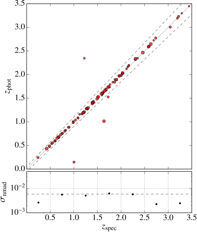
Figure 22: Upper panel: photometric versus spectroscopic redshifts for a sample of $97$ DR14 quasars with $z_{\mathrm{spec}}<3.5$ detected in the miniJPAS field. Larger symbols represent higher $\mathrm{med}(\mathrm{SNR})$. The solid diagonal line indicates $z_{\mathrm{phot}}=z_{\mathrm{spec}}$, and the dashed lines correspond to $z_{\mathrm{phot}}=z_{\mathrm{spec}}\pm 0.05(1+z_{\mathrm{spec}})$. The average photo-$z$ uncertainty, $\sigma_{\mathrm{nmad}}$, is $0.0059$ and the fraction of outliers is $4.1\%$. Bottom panel: photo-$z$ precision as a function of redshift, with the horizontal dashed gray line indicating the average photo-$z$ uncertainty.

6.2.4 Emission line objects

As visually evident from the examples of Fig. 18, the J-PAS filter system allows the detection and characterization of emission lines with equivalent widths larger than a few Å (Martínez-Solaeche et al. 2020, in prep.), from star forming galaxies to AGN and quasars.

H$\alpha$ and [OII]$\lambda$3727 can be used to trace the star forming population from the local universe up to $z\sim$ 1. Weaker lines, such as H$\beta$ and [OIII]$\lambda$5007, can also be easily detected for galaxies with $r<20$ and $z<0.35$, the same magnitude and redshift range of the GAMA survey (Driver et al. 2011). This capability is very important to identify star forming galaxies without, on one hand, the limitations on redshift and/or area coverage typical of narrow-band emission lines surveys, and, on the other hand, the limitations on magnitudes or pre-selection biases of spectroscopic surveys.

AGN and quasars can also be easily identified and their properties characterized with the J-spectra (Abramo et al. 2012; Chaves-Montero et al. 2017). We used miniJPAS data to test a new method that estimates the photo-$z$ of quasars by means of a PCA modeling of the spectral variations (Queiroz et al., in prep.). The eigenspectra of the PCA are computed using as basis a selection of SDSS spectra of broad-line quasars (Yip et al. 2004, but see also Abramo et al. (2012)), and they correspond to the most relevant modes of variation of broad-line quasars. In addition to these eigenmodes we also include a reddening law to allow the eigenspectra’s slope to adjust and better fit reddened quasar spectra. Therefore, our method employs an optimization routine that is tuned to extract the full redshift probability distribution. The quality of the derived photometric redshifts for quasars at $z_{\mathrm{spec}}<3.5$ with $r<22$ is estimated using a subsample of $97$ quasars in the miniJPAS footprint with $\mathrm{med}(\mathrm{SNR})$$\geq 5$, reliable spectral identification in SDSS from Pâris et al. (2018) (mask flag and zWarning flag equal to zero), and for which a visual inspection did not show relevant calibration issues within the miniJPAS observations.

The result is shown in Fig. 22. The estimated average photo-$z$ uncertainty is $0.0059$ and the fraction of outliers is $4.1\%$. We notice that photo-$z$ uncertainty decreases for $z>2$, thanks to the fact that multiple strong emission lines are present within the J-PAS spectral coverage at those high-$z$. With the larger samples provided by J-PAS  we expect to be able to further fine-tune our methods and reach even higher redshift precision.

At $z>2$ J-PAS will also be able to detect and characterize large samples of bright Ly-$\alpha$ emitters (LAEs). The wide spectral coverage of the J-spectra will allow to distinguish those from quasars, making J-PAS highly complementary to surveys studying LAEs with a few narrow bands (e.g., Ouchi et al. 2018) and/or with spectroscopic instruments with limited spectral coverage, such as HETDEX (Hill et al. 2008). In the next section we will discuss the power of J-PAS in performing clustering studies using the expected large samples of emission line galaxies at $z<1$ and quasars and LAEs at $z>2$.

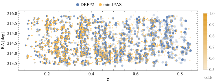
Figure 23: A slice of miniJPAS as mapped by the spectroscopic sample of DEEP2 (blue symbols) and the miniJPAS counterparts (orange symbols), for $r<22.5$. miniJPAS successfully reproduces the pattern of spatial clustering of galaxies unveiled by the spectroscopic DEEP2 survey. The redshifts of miniJPAS sources are given by the best photo-$z$ solution, as described in Sect. 4.2.2. The color shade of the miniJPAS/DEEP2 galaxy pairs is related to the ODDS value of the miniJPAS photo-$z$ solution. The size of the symbols of DEEP2 sources is given by the target photo-$z$ precision, $\sigma_{\rm{NMAD}}=0.003\times(1+z)$, which is reached when the constant-size miniJPAS symbol lies within the DEEP2 one.

6.3 Large scale structure

As already discussed and demonstrated in previous sections, J-PAS was designed as a high-completeness astrophysical survey (Benítez et al. 2009, 2014), with a set of narrow-band filters able to provide photospectra with enough resolution to result in excellent photo-$z$ (see Sect. 4.2.2).

An example of the ability of J-PAS to map the cosmic web is presented in Fig. 23, where we show a slice of the common volume mapped by the spectroscopic sample of DEEP2 and by the photometrically characterized miniJPAS counterparts. Across a wide redshift range, miniJPAS is able to reproduce the pattern of spatial clustering of galaxies unveiled by the spectroscopic DEEP2 survey. The impact of the line-of-sight blurring due to the photo-$z$ errors becomes visible in particular for objects with low values of photo-$z$ accuracy (ODDS). This typically affects scales along the line-of-sight below $\lesssim 50\,h^{-1}$ Mpc. Therefore, J-PAS will be able to accurately map the cosmic structures, from the largest scales to mildly non-linear scales, where most of the cosmological information is encoded. In particular, it will be possible to constrain cosmological models using the filamentary structure of the universe (Tempel et al. 2014; Kitaura et al. 2019).

Due to its large area, high density of objects, as well as accurate photo-$z$, J-PAS will impact cosmology in several different ways. First, since the entire sample of galaxies has photo-$z$ errors lower than $<0.8\%$ (see Sect. 4.2.2), we will be able to extract the scale of baryonic acoustic oscillations (BAO) from galaxy clustering up to $z\sim 1$, both in the transverse and in the radial directions (see, e.g., Chaves-Montero et al. 2018, for the impact of photometric redshifts on clustering measurements). This analysis will produce accurate measurements of the angular-diameter distance $D_{a}(z)$ and the Hubble parameter $H(z)$ (Blake & Glazebrook 2003; Seo & Eisenstein 2003), allowing us to tightly constrain the dark energy equation of state and the other cosmological parameters. Second, being an imaging survey which does not need to rely on the pre-selection of targets, we will be able to measure the shape of the power spectrum (or, equivalently, the correlation function) using many different tracers of the large-scale structure (Seljak 2009; McDonald & Seljak 2009; Abramo et al. 2016): galaxies of different spectral types, colors, luminosities and stellar masses (Arnalte-Mur et al. 2014; Hurtado-Gil et al. 2016; Montero-Dorta et al. 2020), quasars (Abramo et al. 2012), Ly-$\alpha$ emitters (Gurung-López et al. 2019a, b) or even groups and clusters. The multi-tracer character of J-PAS will lead to improved constraints not only on dark energy but also on modified gravity models, primordial non-Gaussianities, and neutrino masses (Abramo & Bertacca 2017). In particular, J-PAS has the potential to provide the most precise determination of the Hubble parameter $H(z)$ and the growth rate $f\sigma_{8}(z)$ for $0.2\leq z\leq 0.6$, outperforming past and upcoming surveys in this redshift range. Dedicated forecast analysis can be found in Costa et al. (2019), Resco et al. (2020) and Aparicio Resco & Maroto (2020, in prep.).

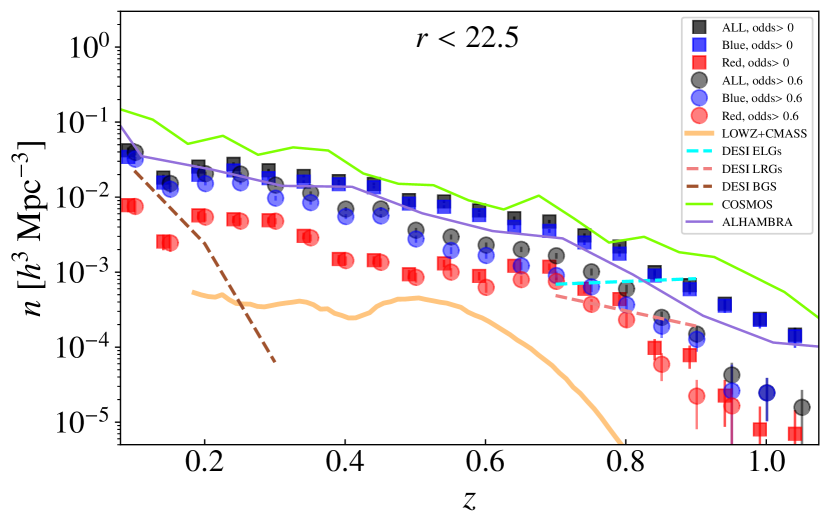
Figure 24: Comoving number density of galaxies in miniJPAS, as a function of redshift. The total galaxy population (dark gray squares) is broken into star-forming (blue squares) and quiescent (red squares). We also apply a cut in photo-$z$ precision (ODDS $>0.6$) (circles, with the same color coding as the squares). We show the number density of galaxies for other surveys like LOWZ+CMASS (orange line), DESI (DESI Collaboration et al. 2016, brown, cyan, and magenta solid lines for, respectively, BCGs, ELGs, and LRGs), ALHAMBRA (Molino et al. 2014, purple line, with an applied cut of $F644W<22.5$, where $F644W$ is a medium-band centred at $6440$Å) and COSMOS (Laigle et al. 2016, green line, with an applied cut of $r<22.5$ ).

Another indicator of the power of J-PAS to constrain cosmology is the signal-to-noise with which we can measure galaxy clustering. For a galaxy with bias $b_{g}$, the amplitude of its clustering in Fourier space is given by $P_{g}=b_{g}^{2}P_{m}(k)$, where $P_{m}(k)$ is the matter power spectrum, whereas the main source of noise is shot (count) noise, $1/\bar{n}_{g}$, where $\bar{n}_{g}$ is the comoving galaxy number density. Since the matter power spectrum at the typical BAO scales ($k_{BAO}=0.1\,h$ Mpc^-1) is of order $P_{m}(k_{BAO})\sim(1+z)^{-2}\times 10^{4}\;h^{-3}$ Mpc³, and galaxy bias is of order $b_{g}\leavevmode\nobreak\ \sim\leavevmode\nobreak\ 1\leavevmode\nobreak\ -\leavevmode\nobreak\ 2$, in order to rise above the level of shot noise a galaxy survey should achieve number densities of $\bar{n}_{g}\gtrsim(1+z)^{2}\times 10^{-4}\,h^{3}$ Mpc^-3. In Fig. 24 we show the estimated (comoving) spatial number density of galaxies at different redshifts for different color and ODDS cuts, based on the photo-$z$ results of miniJPAS (see Sect. 4.2.2) for extended sources with $r<22.5$. These estimates account for the masked regions in the miniJPAS footprint, and incorporate the statistical weights correcting for the stellar contamination (López-Sanjuan et al. 2019b). As expected, we find that blue/late-type galaxies are significantly more abundant than red/early-type ones. Moreover, the photo-$z$ precision of blue galaxies depends significantly on redshift, while the one of red galaxies is approximately constant throughout cosmic ages. Typically, we find number densities in the range $[10^{-3},5\times 10^{-2}]$ $h^{3}$ Mpc^-3, significantly higher than past spectroscopic surveys like LOWZ+CMASS and comparable to the photometric pencil-beam surveys like COSMOS or ALHAMBRA and the upcoming DESI spectroscopic survey. We can select galaxy samples of progressively higher photo-$z$ quality by applying cuts in the ODDS parameter (see details in Section 4.2.2), at the cost of reducing the sample completeness. In Fig. 24 we show that for a cut in ODDS of 0.6, we still obtain fairly large number densities, in the range $[10^{-4},10^{-2}]$ $h^{3}$ Mpc^-3. The redshift precision associated to each ODDS cut depends on redshift, as shown in Fig. 25, where the complicated relation between redshift precision and expected number density of sources is shown for different ODDS cuts and redshift slices. An ODDS cut of 0.6, as used in Fig. 24, generally ensures a relative redshift error of $0.004$ or lower. The previous results and the completeness shown in Fig. 16 suggest that J-PAS will be able to perform very well in the redshift range $0.2<z<0.6$ (Resco et al. 2020; Costa et al. 2019). Indeed, thanks to its unique combination of speed and photo-$z$ accuracy, J-PAS will be able to observe a large number of ELG in this very important redshift range.

In addition to measuring clustering on large scales, J-PAS will also study galaxy correlations at very short scales (a few tens of kiloparsecs, sampling the so-called 1-halo term) due to the high number densities of detected sources. In particular, since J-PAS is not affected by fiber-collision problems in the way spectroscopic surveys are, the small scale limit is set only by the combination of seeing and photometric redshift accuracy. Beyond the standard clustering analyses, the quality of J-PAS data will enable a family of alternative cosmological tests. For instance, the redshift precision of J-PAS will allow us to analyse angular redshift fluctuations (ARF, Hernández-Monteagudo et al. 2019) under narrow redshift shells ($\Delta z\sim 0.01$). This new cosmological observable contains information about the bias and peculiar velocities of the probes, and thus is sensitive to gravity and non-Gaussianity parameters from inflation, among others. A tomographic analysis (like that of Hernández-Monteagudo et al. 2020) would hence provide a detailed view of the redshift evolution of source bias, peculiar velocity amplitudes, and a number of other cosmological quantities that can be derived thereof. At the same time, the combination of ARF with standard 2D angular clustering maps can be naturally cross-correlated with current and future CMB/sub-millimeter maps, and other 2D maps derived from them, like the CMB lensing convergence map, maps of the Cosmic Infrared Background, or maps of the thermal Sunyaev-Zel’dovich effect (Sunyaev & Zeldovich 1972). Given its high number density of galaxies (reaching $>10^{-2}\,h^{3}$ Mpc^-3 at $z<0.5$), J-PAS will also be able to map the cosmic web in rich detail, revealing the pattern of sheets, filaments and voids over an unprecedented volume, and providing a powerful test of the cosmological model as well as of our theory of structure formation (Kitaura et al. 2019). Another potential field where J-PAS may contribute significantly is the study of emission from unresolved sources in different (and narrow) redshift shells: the narrow bands should allow for the isolation of line emitters placed at particular redshifts, even when these lack the required S/N to be identified as sources in the catalogue. Crucial for this intensity mapping (IM) approach (see, e.g., Gong et al. 2011) are the adopted techniques for background removal, which may impact IM signal on the largest scales. Finally, J-PAS will have the unique ability to measure the cosmic shear (see Sect. 6.5.2) in the same volume in which the galaxy power spectrum is measured, thus probing different combinations of the gravitational potentials with two independent observables.

At the highest redshifts ($z>2$), cosmological studies will be possible via quasars and Ly-$\alpha$ emitters (LAEs). Because of their strong emission features, these objects can be easily detected and characterized with the J-spectra. Using miniJPAS, we tested the quasar photo-$z$ uncertainty for objects at $r<22$, being on average $\sim 0.5\%$, but decreasing to $0.3\%$ for objects at $z>2$ (see Sect. 6.2.4). Even at fainter magnitudes (up to $r\sim 23$) we expect to recover complete quasar samples (with a density of $\sim 200$ deg^-2) with $\sim 1\%$ redshift precision, allowing efficient spectroscopic follow-up campaigns. The WEAVE-QSO survey (Pieri et al. 2016) will target $\sim 400k$ J-PAS quasars at $z>2$ which will allow precise Ly-$\alpha$ forest and IGM studies. Finally, at $z>2$, J-PAS will select large samples of LAEs to perform cosmological studies. This will be highly complementary to the HETDEX spectroscopic survey (Hill et al. 2008), as the lower redshift precision of J-PAS will be compensated by the larger area and wider spectral coverage, which allows to easily distinguish LAEs from quasars.

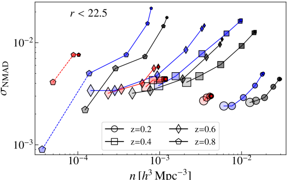
Figure 25: Relation between galaxy number density and corresponding redshift error, as a function of redshift, ODDS cut and galaxy color. Red galaxies, blue galaxies and the full sample are shown, respectively, by red, blue and black lines and symbols. Results are presented in redshift bins of $\Delta z=0.2$, centred at $z=0.2$ (circles), $z=0.4$ (squares), $z=0.6$ (diamonds) and $z=0.8$ (pentagons). For each redshift, the symbols correspond to the cumulative number density for progressively increasing ODDS cuts, with cuts at $ODDS>$0.0, 0.2, 0.4, 0.6, 0.8, 0.9 (for some cuts the symbols are overlapping). The larger the size of the symbols, the larger the ODDS cut (thus the redshift precision). Dashed lines correspond to the regime where we have, in the miniJPAS field, less than 15 galaxies.

6.4 Galaxy clusters

Being the largest gravitationally bound structures in the Universe, galaxy clusters are key to discriminate among the various cosmological models. In particular, they can be used to place constraints on several fundamental parameters such as $\Omega_{m}$ and $\Omega_{\Lambda}$, $w$ and $\sigma_{8}$ (e.g., see Allen et al. 2011, for a review). Ascaso et al. (2016) applied the Bayesian Cluster Finder (Ascaso et al. 2012) and calculated the selection function for J-PAS from N-body+analytical mock catalogues similar to the ones of Merson et al. (2013) adapted to J-PAS. Thanks to the exquisite photo-$z$ that J-PAS can deliver, they found the minimum halo mass threshold for detection of galaxy systems with both $>$80% completeness and purity to be M${}_{halo}\sim 5\times 10^{13}M_{\odot}$ up to z $\sim$ 0.7, outperforming DES (DES Collaboration et al. 2020), ACTpol (Hilton et al. 2018) & SPTpol (Bleem et al. 2020), and comparable to eROSITA (Merloni et al. 2012) and LSST (LSST Science Collaboration et al. 2009) at lower-intermediate redshifts. This is a unique feature of J-PAS, that will allow to expand the study of the evolution of galaxy systems down to galaxy groups. These low-mass systems are particularly interesting and poorly observed at higher redshifts and J-PAS will allow us to clarify many of their unusual properties, among them, to analyse the relative importance of the different mechanisms responsible for the reduction of their measured low baryon fraction (e.g., Dai et al. 2010), for example by comparing stellar loss to intracluster light (Jiménez-Teja et al. 2018, 2019) to IGM ejection (e.g., Bower et al. 2008) due to the energetic excess by central AGN. Moreover, galaxy star formation activity has been suggested to vary over an extended range of environments, measured as a function of galaxy density, and redshift (e.g., Elbaz et al. 2007; Paulino-Afonso et al. 2020). Therefore, the statistical study of galaxy properties in groups will allow us to probe the evolution of galaxies in intermediate environments.

To demonstrate the strength of our multi-band data for the selection of groups and clusters (which hereafter we refer to only as “clusters”), we searched for clusters in miniJPAS within the redshift range $0.05<z<0.8$ with the Voronoi Tessellation (VT) technique (Ramella et al. 2001; Lopes et al. 2004), the Adaptive Matched identifier of Clustered Objects (AMICO, Bellagamba et al. 2018, 2019; Maturi et al. 2019) and the Photo-$z$ Wavelet Cluster Detection Code (PZWav), as described in Euclid Collaboration et al. (2019). AMICO and PZWav are the detection algorithms adopted for the upcoming Euclid survey (Euclid Collaboration et al. 2019). Their use in J-PAS will allow to compare and cross validate the results of the two surveys. All cluster finder algorithms mentioned above found a minimum of 30%-43% of the systems detected in X-rays with a $\leq$ 0.5 Mpc matching scale for $z\leq 0.5$. From these first tests we can detect clusters down to a mass of $\sim 10^{13}M_{\odot}$ and clusters up to redshift $z=0.76$ (mass based on the Chandra X-ray Luminosity scaled mass of Erfanianfar et al. 2013). The cluster catalogue based on miniJPAS data will be presented in an upcoming paper (Maturi & the J-PAS Collaboration 2020, in Prep.). We show here only two illustrative examples. An example of a low mass system is shown in Fig. 26. It is dominated by a bright group galaxy at $z=0.24$ and it has a mass (scaled from X-ray Luminosity) of 2.9$\times 10^{13}M_{\odot}$, typical of groups or poor clusters.

In Fig. 27, instead, we show the most massive cluster detected in the miniJPAS footprint. This is the first cluster that stands out in all cluster finding algorithms used (VT, AMICO, PZWav). It is roughly centred around the Bright Cluster Galaxy at RA:$213.62543$ DEC:$+51.93786$ (one of the two galaxies with spectroscopic redshift in the region, with $z_{s}=0.289$), and we will refer to this cluster as miniJPAS Pathfinder Cluster $2470-1771$, or mJPC $2470-1771$ . It is in the Southwest edge of the miniJPAS field and it has not been analysed previously. The cluster has an unusual central alignment that spans about 500 h${}_{70}^{-1}$ kpc in the plane of the sky, as shown in Fig. 27. Even though this cluster was barely missed by the Chandra observations of the AEGIS field, the XMM-Newton program covering a large area around the Chandra field (PI Merloni) allowed us to derive some X-ray properties relatively well through a a very off-centered 18 ksec XMM pointed observation. We used standard data reduction protocol using the XMM-Newton Science Analysis System (SAS) version xmmsas-v18.0.0. The X-ray spectrum of the hot gas was modeled with an absorbed thermal Bremsstrahlung with emission lines (phabs apec), with redshift fixed on 0.289, corresponding to the Bright Cluster Galaxy (BCG) and hydrogen column density of 1.9 $\times$ 10²⁰ cm^-2. Simultaneous spectral fitting of all imaging spectrometers showed an intracluster gas temperature of $(2.8\pm 0.8)$ keV for a core excised (30 arcsec) region of 80 arcsec radius centred in the X-ray peak. The R₂₀₀, scaled from that X-ray temperature is $\sim 1200\rm{h}_{70}^{-1}$ kpc and a mass M_200c is $\sim$ 3.26$\pm$1.4$\times 10^{14}$ M_⊙. Within that radius miniJPAS finds 29 galaxies within 2000 km s^-1 of the BCG redshift (scale is 4.378 kpc arcsec^-1). Using miniJPAS data alone the mass estimated using richness scaling relation (Lopes et al. 2009), photo-z derived velocity dispersion (Heisler et al. 1985) and the cluster model amplitude returned by the AMICO code is found to be (2.6,4.8,3.7)$\times 10^{14}M_{\odot}$ with (50%,16%,17%) confidence errors respectively. A more detailed analysis of this cluster, including the physical properties of its member galaxies, will be presented in a separate work.

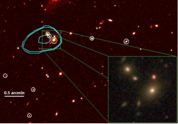
Figure 26: Example of a low-mass cluster (group), mJPC 2241-16656, detected by all three cluster finder algorithms in the miniJPAS/Chandra AEGIS field. The system, dominated by the galaxy SDSS J141719.86+523537.6 is at RA=14:17:20 DEC=+52:35:38 and has photo-$z$=0.238. Overlaid on the i-band image, white circles mark the position of galaxy members (within a window of $\pm$ 4$\sigma_{los}$ - or  840 km/s) within R₂₀₀ (507 h${}_{70}^{-1}$ kpc) (Evrard et al. 1996). These galaxies have membership probability larger than $88\%$ as provided by the AMICO code. The contours in cyan show the extended X-ray emission in the 0.5-2 keV range obtained by the analysis of Chandra data in 0.5dex surface brightness levels levels (for details refer to Erfanianfar et al. 2013). In the bottom right we show a zoom-in of the BCG surroundings for illustration. 1 arcmin corresponds to $\approx$ 230 kpc at the clusters redshift.

6.5 Lensing

The excellent conditions at the OAJ open the window to carry out many studies using gravitational lensing, since not only the shapes of several hundred millions of galaxies will be measured, but their redshifts will also be known with high accuracy.

6.5.1 Strong Lensing

Strong lensing by galaxy clusters offers the opportunity to map the central distribution of dark matter in the cluster, invisible otherwise. Our team has two unique tools to automatically analyse potential cluster strong-lenses found within the J-PAS footprint. The first method was formulated by Zitrin et al. (2012), who showed that by calibrating the effective mass-to-light ratio of cluster members (e.g., using other well-known clusters analysed in HST data), their light-traces-mass method could be operated automatically on large sky surveys, without requiring multiple images as input and relying only on the photometry of identified cluster members (see also Carrasco et al. 2020). This is particularly important because multiple-image constraints for building strong-lens models are typically very hard to identify from the ground. Built on the foundations of this method, Stapelberg et al. (2019) formulated EasyCritics, the second method we use here, which not only estimates the lensing strength of clusters, but also finds them in the data. In Fig.  27 we show the critical curves from the EasyCritics method for a fiducial source at redshift $z_{s}=2$. Note that the calibration used to derive these curves relied on CFHTlens data, not on the miniJPAS data, and thus these curves should only be referred to as an illustration.

In addition to the possibility of J-PAS to find relatively small galaxy-cluster lenses, J-PAS offers unique opportunities to find galaxy-galaxy lenses. Most of these systems are unresolved from the ground with $2.5$ m class telescopes, making the task to find them very difficult. However, using the J-spectra it is in principle possible to find some of these rare systems by looking for outliers corresponding to the overlapping spectra of a foreground lens (the most likely lenses are ellipticals with no emission lines) and a background high-redshift galaxy (common background sources are star forming galaxies at $z>1$, with emission lines). A similar, and successful, effort was conducted using real spectra from SDSS in the SLACS project (Auger et al. 2009)

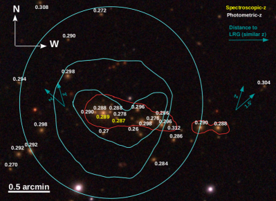
Figure 27: The most massive cluster found in the miniJPAS footprint, centred at RA=213.6254, DEC=51.9379. This cluster is also part of the redMaPPer catalogue where it is listed as a cluster with richness $\lambda=33$. The brightest galaxy has a spectroscopic redshift (from SDSS) of 0.289. Numbers in white next to galaxies indicate the photometric redshift derived from miniJPAS for galaxies with photometric redshifts between $\sim 0.26$ and 0.31. More galaxies in this redshift interval (including some luminous ellipticals) are found at larger distances. The arrows indicate the direction and approximate distance of luminous galaxies found nearby and in this redshift interval. In red are overdrawn the strong lensing critical curves, estimated for fiducial sources at redshift $z_{s}=2$ with the EasyCritics code applied to our data. We also show the X-ray iso-contour emission in the 0.5-2 keV range obtained by the analysis of XMM-Newton (cyan) in steps of 0.5 dex in surface brightness. 1 arcmin corresponds to $\approx$ 200 kpc at the clusters redshift.

6.5.2 Weak Gravitational Lensing

Clusters as massive as mJPC 2470-1771 (Fig. 27) are predicted to show strong lensing effects. Such clusters also produce weak gravitational lensing signals. The photometric depth of J-PAS, in general, makes weak lensing measurements of individual clusters challenging. However, this can be alleviated by performing joint analyses of large samples such as stacked analysis. This has the potential to extract valuable astrophysical and cosmological information from not only massive clusters, but also from low mass ones (see e.g., Fig. 26) and even from individual galaxies.

The OAJ site has shown to have seeing better than 0.8^′′ during 68% of the night time (Moles et al. 2010) and thus can produce images with quality for shear estimation from faint galaxy shape measurements. Given its area and depth, J-PAS has the potential to be one of the main contributors on the fields of cosmic shear, cluster and galaxy-galaxy lensing, prior to the LSST/Euclid era. By using the same procedures and selection criteria as the first year of the HSC-SSP survey (Mandelbaum et al. 2018), we estimated with miniJPAS  that we have an effective number density of source galaxies of $\sim$2.7 arcmin^-2, using the co-added $r$ band images alone, which is a lower limit to what we expect to obtain with J-PAS. This is because the broad band images of the future J-PAS observations are planned to be taken under better conditions (airmass and seeing) than those of miniJPAS. Moreover, with the use of multiple filters for shape measuring we expect to significantly increase the effective number density of source galaxies.

Lensing magnification provides complementary, independent observational alternatives to gravitational shear (Broadhurst et al. 1995; Umetsu et al. 2011; Umetsu 2013). In contrast to the shear-based analysis, measuring the effects of magnification does not require source galaxies to be spatially resolved, whereas it does require accurate photometry across the sky and a stringent flux limit against incompleteness effects. This is where J-PAS has unique advantages against other wide-field surveys.

In the presence of lensing magnification $\mu$ ($\approx 1+2\kappa$ in the weak-lensing regime), the source counts $n(<m)$ for a given magnitude cut $m$ are modified as $n(<m)/n_{0}(<m)=\mu^{2.5s(m)-1}$, with $n_{0}(<m)$ the intrinsic (unlensed) source counts and $s(m)$ the intrinsic count slope, $s(m)=d\log_{10}n_{0}(<m)/dm$. By analysing miniJPAS data, we find that the source counts $n_{0}(<m)$ for a $r$-magnitude-limited sample of background galaxies increase progressively with magnitude down to the completeness limit ($r\sim 22.7$). Since the net effect of magnification bias depends on the count slope $s(m)$, while its signal-to-noise ratio is limited by $n_{0}(<m)$, we will make use of the precise photo-$z$ delivered by J-PAS to optimize the selection of background galaxies in magnitude and redshift space so as to maximize the sensitivity. Therefore, with J-PAS data, we will measure the magnification signal around a large statistical sample of galaxy clusters to obtain a robust mass calibration for cluster cosmology.

7 Summary and Conclusions

In this paper we have presented miniJPAS, a unique 3D survey using the full J-PAS filter system that we have carried out to evaluate the scientific potential of the large J-PAS survey to follow. This first data has allowed us to establish the photometric depth and redshift accuracy that the system can achieve and to test our reduction pipelines for J-PAS. The footprint of miniJPAS was chosen to cover $\sim 1\rm{deg}^{2}$ of the well studied AEGIS field, in all the 56 filters of the J-PAS filter system, plus the four broad bands $u,g,r,i$. The observational strategy adopted allowed us to reach, and often surpass, the desired minimum depths as described in Benítez et al. (2014), obtaining $\rm{mag}_{\rm{AB}}$ between $\sim 22$ and $23.5$ for the NB filters and to $24$ for the BB filters to $5\sigma$ in a $3$ arcsec aperture.

The miniJPAS primary catalogue contains over 64k sources, extracted in the primary $r$ detection band with forced photometry in all other bands. In addition, over 600k sources have been extracted separately in the individual bands, generating catalogues that are particularly interesting for the detection of extreme line emitters over the wide spectral range covered by the narrow band filters. We estimate the full miniJPAS catalogue to be complete up to $r=23.6$ AB for point-like sources and $r=22.7$ AB for extended sources. Photometric redshifts have been derived using a customised version of LePhare, modified to work with a larger number of filters and higher resolution in redshift than typically required for broad-band photometry. We have demonstrated here that the J-PAS filter system is able to reach sub-percent precision in photo-$z$  for all sources brighter than mag$\sim 22.5$. The target precision of $0.3\%$ is reached for about half the sources, and subsamples with redshift precision as high as $0.2\%$ can also be extracted by performing appropriate cuts from the photo-$z$ outputs.

All data, from images to catalogues and value-added data products from this miniJPAS survey have been publicly released at the end of 2019 and are available in the J-PAS data portal. Data can be accessed via a variety of tools: sky navigator , object list searches and ADQL queries.

The analysis of miniJPAS  has highlighted several examples of the many scientific applications possible with the upcoming large J-PAS. We have shown how the J-spectra can be used to characterize a very wide variety of sources, from galactic objects to high redshift quasars, thanks to the photometric detection of absorption and emission features readily visible in our spectral energy distributions. We have demonstrated that stellar population studies can be carried out up to $z\sim 1$ and the that detailed morphology and structural properties of galaxies can be analysed combining the multi-color information. We have shown the capability of J-PAS as effectively a massive IFU survey, of cosmologically useful spectral resolution over an unprecedentedly large FoV. The accurate photo-$z$ achieved are key to the study of the large scale structure, including baryon acoustic oscillations as well as the shape and evolution of the power spectrum of galaxies and clusters. It is now clear from our survey that galaxy samples with sub-percent redshift precision and a number density as high as $>10^{-2}\,h^{3}$ Mpc^-3 can be selected at $z<0.4$, and with a number density exceeding $10^{-4}\,h^{3}$ Mpc^-3 at $0.4<z<0.9$, as well as a near-complete sample of $r<23$ quasars at redshifts $z>2$. We have shown that secure identification of clusters and groups of galaxies can be made within this redshift range because our redshift precision means there is minimal contamination by non members. Furthermore, we have shown with miniJPAS that weak lensing is detectable for individual massive clusters and can be stacked for groups, allowing us to track the mass evolution of clusters to unprecedented depth, providing a self-contained evolution of the mass function with the J-PAS survey.

We conclude that miniJPAS has demonstrated the capability of the J-PAS filter system to deliver accurate classification of stars and extragalactic sources, and the unambiguous redshift determination of tens of thousands of galaxies per squared degree. miniJPAS is only a tiny wedge of the sky that J-PAS will probe, as J-PAS will surpass miniJPAS by more than three orders of magnitude in terms of area and hence number of sources and volume surveyed. The full survey will provide a contiguous 3D map of the Northern sky to $z\sim 0.9$, offering the opportunity to study galaxy evolution and the large scale structure of the Universe over a large fraction of the cosmological volume and opening the window to serendipitous discoveries.

Appendix A Log of miniJPASobservations

In this appendix we provide some information on the data aquisition. More details on each tile can be found in the database in the ADQL table minijpas.TileImage. In Table 11 we indicate the number of exposures taken for each filter in each pointings (red: miniJPAS-AEGIS1, blue: miniJPAS-AEGIS2, green: miniJPAS-AEGIS3, orange: miniJPAS-AEGIS4). Different groups of filters have been observed in different observational blocks (FW$\#$), following the chosen strategy of filter changes in the JPAS-PF filter wheel (see Sect. 2.4). Total exposure times per pointing are reported in the last column.

Table 11: Log of miniJPAS observations. Number of exposures taken for each filter, for each pointing and in each observing epoch (the dates correspond to the day a new set of filter was installed on the filter wheel). The last two columns provide the total number of exposures used in the final co-added images and the total exposure time. Red: miniJPAS-AEGIS1, blue: miniJPAS-AEGIS2, green: miniJPAS-AEGIS3, orange: miniJPAS-AEGIS4.

FILTER	FW01	FW02	FW03	FW04	FW05	FW06	FW07	FW08	FW09	FW10	FW11	FW12	FW13	TOTAL	TOTAL
	2018-04-27	2018-05-18	2018-06-18	2018-06-28	2018-07-11	2018-07-20	2018-08-03	2018-08-14	2018-08-24	2018-09-25	2018-10-09	2019-02-05	2019-07-11	$N_{\textrm{img}}$	$t_{\textrm{exp}}$(s)
uJAVA												16, 8, 8, 18		16, 8, 8, 18	1920, 960, 960, 2160
uJPAS								4, 4, 4, 4						4, 4, 4, 4	480, 480, 480, 480
gSDSS	16, 16, 16, 16													16, 16, 16, 16	480, 480, 480, 480
rSDSS	6, 27, 1, 19	31	16, 3	10, 16, 15	4									37, 37, 37, 37	1110, 1110, 1110, 1110
iSDSS	16, 16, 16, 16												16, 32	16, 16, 32, 48	480, 480, 960, 1440
J0378								4, 8, 4, 4						4, 8, 4, 4	480, 960, 480, 480
J0390		11, 4, 4, 4										16, 8, 8, 8		27, 12, 12, 12	3240, 1440, 1440, 1440
J0400				9, 4, 4, 8										9, 4, 4, 8	1080, 480, 480, 960
J0410						16, 12, 8, 4								16, 12, 8, 4	1920, 1440, 960, 480
J0420			4, 4, 4, 8								4, 12			4, 4, 8, 20	480, 480, 960, 2400
J0430							10, 4, 4, 4							10, 4, 4, 4	1200, 480, 480, 480
J0440					8, 4, 4, 8								4, 8, 4	8, 8, 12, 12	960, 960, 1440, 1440
J0450								9, 8, 4, 8						9, 8, 4, 8	1080, 960, 480, 960
J0460		10, 4, 5, 9										8, 8, 8, 8		18, 12, 13, 17	2160, 1440, 1560, 2040
J0470				8, 4, 4, 8										8, 4, 4, 8	960, 480, 480, 960
J0480						12, 12, 8, 8								12, 12, 8, 8	1440, 1440, 960, 960
J0490			4, 4, 4, 8								12			4, 4, 4, 20	480, 480, 480, 2400
J0500							4, 4, 4, 4							4, 4, 4, 4	480, 480, 480, 480
J0510					8, 4, 4, 8									8, 4, 4, 8	960, 480, 480, 960
J0520								8, 8, 8, 8						8, 8, 8, 8	960, 960, 960, 960
J0530		12, 4, 4, 4											4, 8, 4	12, 8, 12, 8	1440, 960, 1440, 960
J0540				4, 4, 4, 4										4, 4, 4, 4	480, 480, 480, 480
J0550						12, 12, 9, 8								12, 12, 9, 8	1440, 1440, 1080, 960
J0560			8, 4, 4, 8								8			8, 4, 4, 16	960, 480, 480, 1920
J0570							4, 4, 4, 4							4, 4, 4, 4	480, 480, 480, 480
J0580					8, 4, 4, 8									8, 4, 4, 8	960, 480, 480, 960
J0590								4, 8, 8, 8			12, 4			16, 8, 12, 8	1920, 960, 1440, 960
J0600		5, 4										8, 8, 8, 8		13, 8, 8, 12	1560, 960, 960, 1440
J0610				4, 4, 4, 4										4, 4, 4, 4	480, 480, 480, 480
J0620						8, 8, 8, 12								8, 8, 8, 12	960, 960, 960, 1440
J0630			4, 4, 4, 8								4			4, 4, 4, 12	480, 480, 480, 1440
J0640							8, 9, 11, 8							8, 9, 11, 8	960, 1080, 1320, 960
J0650					8, 4, 4, 8									8, 4, 4, 8	960, 480, 480, 960
J0660	8, 12, 4, 5											8, 8, 8, 8		16, 20, 12, 13	1920, 2400, 1440, 1560
J0670		12, 4, 4, 6										8, 8, 4, 4		20, 12, 8, 10	2400, 1440, 960, 1200
J0680				4, 4, 4, 4									4, 8, 4	4, 8, 12, 8	480, 960, 1440, 960
J0690						8, 8, 8, 9							4, 8, 4	8, 12, 16, 13	960, 1440, 1920, 1560
J0700			4, 4, 4, 8											4, 4, 4, 8	480, 480, 480, 960
J0710							4, 4, 4, 4							4, 4, 4, 4	480, 480, 480, 480
J0720					8, 4, 4, 8									8, 4, 4, 8	960, 480, 480, 960
J0730								4, 8, 7, 8			8			12, 8, 7, 8	1440, 960, 840, 960
J0740		12, 4, 4, 4											4, 8, 4	12, 8, 12, 8	1440, 960, 1440, 960
J0750				4, 4, 4, 4										4, 4, 4, 4	480, 480, 480, 480
J0760						9, 4, 8, 9								9, 4, 8, 9	1080, 480, 960, 1080
J0770			4, 4, 4, 8											4, 4, 4, 8	480, 480, 480, 960
J0780							8, 4, 4, 4							8, 4, 4, 4	960, 480, 480, 480
J0790					8, 4, 4, 8									8, 4, 4, 8	960, 480, 480, 960
J0800									8, 18, 8, 8					8, 18, 8, 8	960, 2160, 960, 960
J0810									8, 8, 8, 8					8, 8, 8, 8	960, 960, 960, 960
J0820									8, 8, 8, 8					8, 8, 8, 8	960, 960, 960, 960
J0830									16, 8, 16, 8					16, 8, 16, 8	1920, 960, 1920, 960
J0840									16, 8, 8, 8					16, 8, 8, 8	1920, 960, 960, 960
J0850									13, 8, 8, 8					13, 8, 8, 8	1560, 960, 960, 960
J0860	12, 12, 4, 4													12, 12, 4, 4	1440, 1440, 480, 480
J0870										12, 16, 20, 8				12, 16, 20, 8	1440, 1920, 2400, 960
J0880										12, 13, 12, 8				12, 13, 12, 8	1440, 1560, 1440, 960
J0890										12, 8, 12, 8				12, 8, 12, 8	1440, 960, 1440, 960
J0900										12, 8, 12, 8				12, 8, 12, 8	1440, 960, 1440, 960
J0910										4, 8, 4, 8				4, 8, 4, 8	480, 960, 480, 960
J1007										4, 7, 12, 8				4, 7, 12, 8	480, 840, 1440, 960

Appendix B Background correction

Extending the discussion from Sect. 3.1, here we provide more technical details on the background treatment of the miniJPAS images. In particular, we describe a background correction derived from the illumination correction and a “superbackground” correction, as we call it.

B.1 Background correction derived from illumination correction

The illumination correction is becoming a standard step in the image reduction chain when the acquisition system involves large FoVs and/or includes lenses like field correctors. Such telescopes are prone to suffer from illumination issues. Their origin is explained in Andersen et al. (1995). Nowadays, projects involving that type of telescopes take that effect into account (e.g. DES, Bernstein et al. (2017) and SDSS, Betoule et al. (2013)). The approach adopted for the illumination correction in the OAJ reduction pipeline is based on Manfroid (1995). It requires the acquisition of a set of specific observations. In the case of miniJPAS  these were planned during miniJPAS observing campaign. From these observations a master illumination correction image (ICOR, hereafter) was constructed for each filter and this was applied to the images just after the flat field correction. However, images corrected by the illumination correction showed a background pattern not visible after the preceding flat field correction.

Before continuing with the description of the procedure aiming at removing this apparent worsening of the images after the illumination correction, let us explain its origin.

Due to the optics of the system, a flat illumination arriving to the telescope can result in a non uniform distribution of light in the detector. This affects the scientific images in two ways. First, they show a non uniform background pattern which is an additive component that should be subtracted. Second, it affects the flat field correction. If not taken into account, the non uniform distribution of light in the flat field images is assumed as a variation of efficiency (which is not). This has two effects on the scientific images after being divided by the master flat. First, it introduces a 2D variation of the photometry of the objects (i.e. a 2D variation of the photometric zero point). This is the effect corrected by the ICOR. The second effect is to apparently remove the previous background pattern of the scientific images. However, this background should be corrected by subtraction and not by division and, therefore, this apparent background removal is actually wrong. And, in fact, any additive background present in the raw image, should be present in the images after flat field correction. That is the reason why after the illumination correction, which corrects the flat field itself, the original additive background pattern present in the raw image reappears in the scientific image.

Then, knowing that there is a background component of the images which has the same spatial distribution as the ICOR and that it is an additive component, a new background correction is computed having the 2D distribution of the ICOR and an average value of the average background of the target image. This background correction is subtracted just after applying ICOR resulting in an reduced image with flatter background and flatter zero point.

Finally, to check that this background subtraction did not affect the actual photometry of the objects of the images, we processed the individual images used for constructing an ICOR, controlling that the differences in the photometry of individual objects observed in different images were compatible with zero.

B.2 Superbackground correction

After the background subtraction from the ICOR, many single frames still display background patterns whose spatial distribution made them difficult to be properly managed in a massive automatic way during the source detection process, i.e. with SExtractor. These patterns have two main characteristics that make the correction complex: presence of strong background gradients and strong temporal variability of the patterns, either in intensity or spatial distribution.

Under the assumptions that these patterns are instrumental, and therefore do not depend on the sky position (at least for close enough pointings), and that they are stable in time scales of few minutes, we can consider that images taken close in time (with the same filter) present the same background pattern. Therefore, a median combination of scientific images with celestial objects in different CCD positions should keep the background pattern while removing the real astrophysical objects. This is a procedure analogue to the construction of master fringing images or superflat images, for this reason we dubbed these background images as “superbackground images” (SBGK, hereafter).

The observational strategy of miniJPAS in which the single exposures of the same pointing and same filter were taken with small dithering and one after the other, introduced one problem and provided an advantage. First, to not subtract light of real objects when constructing the SBGK, it is necessary to avoid to have celestial objects falling in the same parts of the images combined to construct the SBGK. Due to the temporal variation of the patterns (with detected changes on scales of several minutes), it was not possible to combine images of the same filter and different pointings, since they already showed changes in the background. Therefore, we were left with the only possibility of having to use the images of the same pointing and, due to the small dithering pattern, the chances of having areas of the image covered by actual objects were high, in particular for larger diffuse objects. To minimize this possibility, before combining the images, the objects detected in a preliminary reduction without SBKG correction were masked with masks a bit larger than the actual detected size of the object to take into account extended diffuse light. This masking procedure was fine-tuned until it was checked that there were no residuals of extended galaxies in the SBGK (for bright saturated stars we allowed for light of their halos to be in the SBKG). In the specific case of miniJPAS data, being a cosmological field devoid of large galaxies (i.e., galaxies occupying a large area of the CCD), the possible oversubtraction of background due to this procedure was not a big issue, although for the studies of faint extended studies this has to be kept in mind.

In summary, the SBKG construction consisted, first, in identifying the images to be combined. That was done taking advantage that exposures of the same pointing and same filter were done consecutively and, therefore, we could consider that in the interval between the first and last exposure the background pattern was stable (although in few ocassions we detected that this wasn’t the case and some residuals were left). Then, objects were masked and images median-combined. Finally, the resulting image was smoothed using SExtractor. The last step was to subtract the SBKG to the individual scientific frames.

Again, in order to verify that the SBGK correction did not affect the photometry of the objects, we simulated the construction of an ICOR (a procedure that by construction shows changes in photometry of object across the CCD) applying all the corrections to the images to be used, finding that the resulting map was compatible with no correction.

Appendix C SExtractor’s parameters

Source detection and basic parameters of the objects in the images have been done using SExtractor Bertin & Arnouts (1996). Details on how SExtractor works can be found either in Bertin & Arnouts (1996) and in the SExtractor User’s Manual. In Table 12 we provide the list of parameters that have been used to obtain the photometric catalogues that are the base of this data release. We only list those parameters that are common to all the images. Other parameters, such as CATALOG_NAME, CHECKIMAGE_NAME, are obviously specific to each image and are not included in the table.

Table 12: List of SExtractor’s parameters used to construct the miniJPAS source catalogues.

SExtractorparameter	value
ANALYSIS_THRESH	2.0
BACKPHOTO_THICK	24
BACKPHOTO_TYPE	LOCAL
BACK_FILTERSIZE	3
BACK_FILTTHRESH	0.0
BACK_SIZE	512
BACK_TYPE	AUTO
BACK_VALUE	0.0,0.0
CLEAN	Y
CLEAN_PARAM	1.0
DEBLEND_MINCONT	0.005
DEBLEND_NTHRESH	32
DETECT_MINAREA	5
DETECT_THRESH	0.9 (dual-mode) / 2 (single-mode)
DETECT_TYPE	CCD
FILTER	Y
FILTER_NAME	gauss_3.0_5x5.conv
GAIN_KEY	GAIN
MASK_TYPE	CORRECT
PHOT_AUTOAPERS	0.0,0.0
PHOT_AUTOPARAMS	2.5,3.5
PHOT_FLUXFRAC	0.5
PHOT_PETROPARAMS	2.0,3.5
PIXEL_SCALE	0.2267
STARNNW_NAME	default.nnw
THRESH_TYPE	RELATIVE
VERBOSE_TYPE	NORMAL
WEIGHT_GAIN	Y
WEIGHT_THRESH	0,0
WEIGHT_TYPE	MAP_WEIGHT,MAP_WEIGHT