Fully dispersive Boussinesq models with uneven bathymetry

Abstract

Three weakly nonlinear but fully dispersive Whitham-Boussinesq systems for uneven bathymetry are studied. The derivation and discretization of one system is presented. The numerical solutions of all three are compared with wave gauge measurements from a series of laboratory experiments conducted by Dingemans [13]. The results show that although the models are mathematically similar, their accuracy varies dramatically.

1 Introduction

In coastal engineering, Boussinesq models are used to approximate full Euler or Navier-Stokes equations which are numerically intractable on large scales. The main assumptions on the waves to be represented by approximate Boussinesq-type models are that they be of small amplitude and long wavelength when compared to the undisturbed depth of the fluid. As explained in [24], classical Boussinesq models are able to accurately describe waves up to a wavelength-to-depth ratio of $kh\sim 1.3$, where $k=2\pi/\lambda$ is the wavenumber, $\lambda$ is the wavelength, and $h$ is the local depth. On the other hand, in many practical applications, it is desirable to be able to treat shorter waves or waves in deeper water, and the development of coastal models has long been focused on obtaining models allowing closer approximation of waves in deeper water.

One of the first results in this direction was given in [37], where a KdV equation with improved dispersion properties was found. In [24, 26], two-dimensional Boussinesq equations with improved dispersion and bathymetry were put forward. The dispersion relation was further improved by [28], and in many subsequent articles. Current models are able to treat smaller wavelength-to-depth ratios than the traditional Boussinesq models, up to about $kh\sim 30$ [7, 25, 32]. However, one drawback with these high-order systems is that they tend to become very cumbersome to represent in writing and to implement numerically. In addition, many numerical fixes are used (sometimes tacitly) because the modifications done in order to improve linear dispersion and treatment of bathymetry sometimes introduce instabilities.

In the present work, we consider a class of fully dispersive Boussinesq systems. These systems are developed using an idea of Whitham [36] who put forward the original nonlinear fully dispersive equation

$$\eta_{t}+\frac{3}{2}\frac{c_{0}}{h}\eta\eta_{x}+\int_{-\infty}^{\infty}\mathcal{K}_{h}(y)\eta_{x}(x-y)\,dy=0,$$ (1.1)

where $h$ is the undisturbed depth of the fluid, $c_{0}=\sqrt{gh}$ is the corresponding long-wave speed, and $g$ is the gravitational acceleration. The integral kernel $\mathcal{K}_{h}$ is given in terms of the Fourier transform and the linear phase speed $c(\xi)$ by

$$\mathcal{F}\mathcal{K}_{h}(\xi)=c(\xi)={\textstyle{\sqrt{g\frac{\tanh(h\xi)}{\xi}}}}.$$ (1.2)

The convolution can be thought of as a Fourier multiplier operator and (1.2) represents the Fourier symbol of the operator. Indeed, using the notation $D=-i\partial_{x}$, the integral operator can be written in the form $\sqrt{gh\mathcal{K}}$, where

$$\mathcal{K}=\frac{\tanh(hD)}{hD}.$$ (1.3)

The linearization of equation (1.1) gives an exact unidirectional representation of the linear dispersion relation of the free-surface water-wave problem. The fidelity of solutions of this equation has been tested against numerical solutions of the the Euler equations [27] and measurements from wave tank experiments [8]. In recent work, the Whitham equation, (1.1), has been generalized to systems of equations allowing for bi-directional wave propagation. Essentially, three different forms of the equations have been put forward [1, 14, 19], and these have also been tested against laboratory data from experiments with constant depth, see [8].

We consider the influence of bathymetry, which is an essential feature from the point of view of coastal engineering. In fact, the model found in [1] already featured nontrivial bathymetry, but the bathymetric terms were somewhat simplified. Here, we investigate the bidirectional Whitham-type system from [1] with full bathymetric terms as well as capillarity in the form

$$\partial_{t}\eta =-h\mathcal{K}\partial_{x}(1+\frac{\tau}{g}D^{2})u-\partial_{x}(\eta u)-\partial_{x}L(\beta)D^{-1}u,$$ (1.4)

$$\partial_{t}u =-g\partial_{x}\eta-\partial_{x}u^{2}/2,$$

where the parameter $\tau$ represents the coefficient of surface tension. The unknowns $\eta$ and $u$ are real-valued functions of the spatial variable $x\in\mathbb{R}$ and the temporal variable $t\in[0,\infty)$. They represent the surface displacement of the fluid and the horizontal velocity component defined by $u=\partial_{x}\Phi$ where $\Phi(x,t)$ is the surface trace of the fluid’s velocity potential $\phi(x,z,t)$. The bathymetry operator $L(\beta)$ was introduced in [12] and has the form

$$L(\beta)=-C(\beta)^{-1}A(\beta),$$ (1.5)

where the operators $A(\beta)$ and $C(\beta)$ are defined by

$$A(\beta)f=\int e^{ikx}\sinh\big{(}\beta(x)k\big{)}\operatorname{sech}(hk)\widehat{f}(k)dk=\int e^{ik(x-s)}\frac{\sinh\big{(}\beta(x)k\big{)}}{\cosh(hk)}f(s)dsdk,$$ (1.6)

$$C(\beta)f=\int e^{ikx}\cosh\big{(}(-h+\beta(x))k\big{)}\widehat{f}(k)dk=\int e^{ik(x-s)}\cosh\big{(}(-h+\beta(x))k\big{)}f(s)dsdk.$$ (1.7)

If the bottom is flat, then $\beta(x)=0$ and $L(\beta)=0$, and in this case, it was proven in [30] that this system is well-posed if the surface displacement is strictly positive. Additionally, it was suggested that this system is ill-posed in general. Numerical results corroborating these well-posedness/ill-posedness statements were detailed in [10, 15]. However, as will be shown below, these result do not seem to have a bearing on the numerical experiments presented here. Indeed, it was shown in [8] that the flat-bottom version of this system represents a more accurate model of the evolution of initial waves of depression over a flat bottom than the KdV equation and even the higher-order Serre-Green-Naghdi system.

The system has the conserved Hamiltonian function

$$\mathcal{H}=\frac{1}{2}\int_{\mathbb{R}}\Big{(}g\eta^{2}+hu\mathcal{K}(1+\frac{\tau}{g}D^{2})u+uLD^{-1}u+\eta u^{2}\Big{)}dx,$$ (1.8)

and in terms of $\mathcal{H}$ , the system can be written in the form

$$\eta_{t}=-\partial_{x}\frac{\delta\mathcal{H}}{\delta u},$$ (1.9)

$$u_{t}=-\partial_{x}\frac{\delta\mathcal{H}}{\delta\eta}.$$

It was shown in [27] that (1.8) can be viewed as a fully-dispersive approximation of the total energy of the full water-wave problem.

A different model system was proposed in the case of a flat-bottom in [19]. In the presence of bathymetry and capillarity, the system has the form

$$\partial_{t}\eta =-h\partial_{x}u-\partial_{x}(\eta u)-\partial_{x}L(\beta)D^{-1}u,$$ (1.10)

$$\partial_{t}u =-g\mathcal{K}\partial_{x}(1+\frac{\tau}{g}D^{2})\eta-\partial_{x}u^{2}/2,$$

where $\eta$ is the free-surface displacement, and $u=\partial_{x}\Phi(x,t)$ is the horizontal velocity component as before. The system (1.10) also has a Hamiltonian structure. Indeed, the system can be written in the form

$$\eta_{t}=-\partial_{x}\frac{\delta\mathcal{H}}{\delta u},$$ (1.11)

$$u_{t}=-\partial_{x}\frac{\delta\mathcal{H}}{\delta\eta},$$

with the Hamiltonian

$$\mathcal{H}=\frac{1}{2}\int_{\mathbb{R}}\Big{(}g\eta\mathcal{K}(1+\frac{\tau}{g}D^{2})\eta+hu^{2}+uLD^{-1}u+\eta u^{2}\Big{)}dx.$$ (1.12)

However this Hamiltonian is not an approximation of the Hamiltonian of the water-wave problem in the context of the Craig-Sulem-Zakharov formulation (see for example[21]). It was shown in [19] that periodic traveling-wave solutions are spectrally unstable with respect to long-wave perturbations due to the modulational instability.

A third model can be obtained by imposing the operator $\mathcal{K}$ also on the nonlinear parts of (1.10). This gives the system

$$\partial_{t}\eta =-h\partial_{x}v-\mathcal{K}\partial_{x}(\eta v)-\partial_{x}L(\beta)D^{-1}\mathcal{K}^{-1}v,$$ (1.13)

$$\partial_{t}v =-g\mathcal{K}\partial_{x}(1+\frac{\tau}{g}D^{2})\eta-\mathcal{K}\partial_{x}v^{2}/2.$$

The unknowns $\eta$ and $v$ are real-valued functions of the spatial variable $x\in\mathbb{R}$ and the temporal variable $t\in[0,\infty)$. They represent the surface displacement of the fluid and the “velocity” defined by $v=\mathcal{K}\partial_{x}\Phi$ where $\Phi(x,t)$ is the surface trace of the fluid’s velocity potential $\phi(x,z,t)$. The system given in equation (1.13) is a conservative Hamiltonian system. In $\eta,v$ variables the Hamiltonian functional, $\mathcal{H}(\eta,v)$, has the form

$$\mathcal{H}=\frac{1}{2}\int_{\mathbb{R}}\Big{(}g\eta(1+\frac{\tau}{g}D^{2})\eta+hv\mathcal{K}^{-1}v+v\mathcal{K}^{-1}LD^{-1}\mathcal{K}^{-1}v+\eta v^{2}\Big{)}dx,$$ (1.14)

with the structure map

$$J_{\eta,v}=\begin{pmatrix}0&-\mathcal{K}\partial_{x}\\ -\mathcal{K}\partial_{x}&0\end{pmatrix}.$$

Thus, the Hamiltonian system is given by

$$\eta_{t}=-\mathcal{K}\partial_{x}\frac{\delta\mathcal{H}}{\delta v},$$ (1.15)

$$v_{t}=-\mathcal{K}\partial_{x}\frac{\delta\mathcal{H}}{\delta\eta}.$$

The system (1.13) was first introduced in [15] in the context of an even bed and without capillarity, and it was shown in [14, 17] that in this simpler case, the system is mathematically well-posed. It was also shown that the simplified system admits solitary-wave solutions [16].

The three systems detailed above are similar, yet have very different mathematical properties. In this article, we aim to study these systems from a modeling point of view, in order to determine which of these systems holds most promise as a water-wave model. We start by giving a derivation of (1.13) from the full water wave problem by applying the Hamiltonian long-wave approximation presented in [11]. In fact, the derivation of these three systems is similar, and we chose to show the derivation of (1.13) because it has appeared most recently in the literature. The derivation is based on an approximation of the Hamiltonian which approximates the total energy of the water-wave problem based on the full Euler equations.

2 Hamiltonian formulation

Consider an inviscid, incompressible, and irrotational fluid with domain $x\in\mathbb{R}$, $-h+\beta(x)<z<\eta(x,t)$. Its motion is described by the Laplace equation

$$\partial_{x}^{2}\phi+\partial_{z}^{2}\phi=0,$$

in the fluid domain, the Neumann boundary condition

$$\partial_{n}\phi=0,$$

at the bottom, $z=-h+\beta(x)$, indicating the fact that the bottom is impenetrable, the kinematic condition

$$\partial_{t}\eta+(\partial_{x}\eta)\partial_{x}\phi-\partial_{z}\phi=0,$$

at the free surface, $z=\eta(x,t)$, and the Bernoulli equation including surface tension

$$\partial_{t}\phi+\frac{1}{2}|\nabla\phi|^{2}+g\eta-\tau\partial_{x}\Big{(}\frac{\partial_{x}\eta}{\sqrt{1+(\partial_{x}\eta)^{2}}}\Big{)}=0,$$

also at the free surface.

In order to reduce this system, we introduce the trace of the velocity potential at the free surface, $\Phi(x,t)=\phi(x,\eta(x,t),t)$, and the Dirichlet-Neumann operator, $G(\eta,\beta)$, via the formula

$$G(\eta,\beta)\Phi=\sqrt{1+(\partial_{x}\eta)^{2}}\partial_{n}\phi,$$ (2.1)

where $\partial_{n}\phi$ is the projection of the surface fluid velocity on the outward normal vector. For a more detailed definition of $G(\eta,\beta)$ taking into account the appropriate asymptotic conditions on $\phi$, we refer the reader to [2, 21]. Using the Dirichlet-Neumann operator, the full problem reduces to

$$\partial_{t}\eta =G(\eta,\beta)\Phi,$$ (2.2)

$$\partial_{t}\Phi =-g\eta+\tau\partial_{x}\Big{(}\frac{\partial_{x}\eta}{\sqrt{1+(\partial_{x}\eta)^{2}}}\Big{)}-\frac{1}{2}(\partial_{x}\Phi)^{2}+\frac{((\partial_{x}\eta)\partial_{x}\Phi+G(\eta,\beta)\Phi)^{2}}{2(1+(\partial_{x}\eta)^{2})},$$

posed on the free surface. A pair $(\eta,\Phi)$ that solves system (2.2) completely describes the surface waves. A drawback of this formulation is that the Dirichlet-Neumann operator implicitly depends on the surface elevation $\eta$. Zakharov [38] showed that system (2.2) has the Hamiltonian structure

$$\partial_{t}\eta=\frac{\delta\mathcal{H}}{\delta\Phi},$$ (2.3)

$$\partial_{t}\Phi=-\frac{\delta\mathcal{H}}{\delta\eta},$$

with total energy

$$\mathcal{H}(\eta,\Phi)=\frac{1}{2}\int_{\mathbb{R}}\Big{(}g\eta^{2}+\Phi G(\eta,\beta)\Phi+{\textstyle\frac{2\tau(\partial_{x}\eta)^{2}}{1+\sqrt{1+(\partial_{x}\eta)^{2}}}}\Big{)}dx,$$ (2.4)

serving as the Hamiltonian. The first term in the integral, which we denote $\mathcal{H}_{p}$, represents the potential energy, the second term, $\mathcal{H}_{k}$, represents the kinetic energy, and the last term, $\mathcal{H}_{\tau}$, represents the capillary energy. The surface water wave problem can be further simplified by approximating the Dirichlet-Neumann operator using different explicit expressions. We also note that there are different Hamiltonian formulations for this problem, such as detailed for example in [29]

3 Derivation

It is well known that the Dirichlet-Neumann operator can be expanded in a power series in $\eta$, see for example, [12]. In the weakly nonlinear framework considered here, we keep the first two terms in this power series, and disregard all higher-order terms. In other words, we make the approximation $G\approx G^{0}+G^{1}$, where

$$G^{0}=D\tanh(hD)+DL,$$ (3.1)

$$G^{1}=D\eta D-G^{0}\eta G^{0}.$$

Recall that the operator $L=L(\beta)$ defined above in equation (1.5) represents bathymetric effects. Note also that $G^{0}=G(0,\beta)$ is symmetric, i.e. for any real-valued functions $f_{1}$ and $f_{2}$ belonging to the domain of $G^{0}$ the following identity

$$\int_{\mathbb{R}}(G^{0}f_{1})(x)f_{2}(x)dx=\int_{\mathbb{R}}f_{1}(x)(G^{0}f_{2})(x)dx,$$

holds. This follows from the definition of the Dirichlet-Neumann operator and Green’s formula. In particular, $DL$ is symmetric and therefore $LD^{-1}$ is also symmetric. This fact will figure into the analysis below.

In order to simplify the system, we introduce four nondimensional parameters: $\varepsilon=a_{s}/h$, $\mu=h^{2}/\lambda^{2}$, $\gamma=a_{b}/h$, and $\varkappa=\tau/(gh^{2})$ that measure nonlinearity, shallowness, bathymetric variation, and capillarity, respectively. Here $a_{s}$ represents a characteristic surface amplitude, $a_{b}$ represents a characteristic bathymetric variation, and $\lambda$ represents a characteristic surface wavelength. We assume $\mu\ll 1$. Generally in the Boussinesq regime, $\varepsilon=\mathcal{O}(\mu)$. However below, it is sufficient to assume only $\epsilon=o(1)$. Additionally, we assume that the bathymetric variation does not have to be small by allowing $\gamma=\mathcal{O}(1)$.

Linear theory suggests defining $t_{0}=\lambda/\sqrt{gh}$ and $\Phi_{0}=a_{s}\lambda\sqrt{gh}/h$ to be the units for time and velocity potential. Therefore, let $\tilde{x}=x/\lambda$, $\tilde{\eta}=\eta/a_{s}$, $\tilde{\beta}=\beta/a_{b}$, $\tilde{t}=t/t_{0}$ and $\tilde{\Phi}=\Phi/\Phi_{0}$ be dimensionless variables. Similarly, it is convenient to take the units of energy to be $\mathcal{H}_{0}=ga_{s}^{2}\lambda.$ The dimensionless Dirichlet-Neumann operator, $G_{\mu}$, is defined by

$$G_{\mu}\left(\varepsilon\tilde{\eta},\gamma\tilde{\beta}\right)\tilde{\Phi}=\frac{h}{\Phi_{0}}G(\eta,\beta)\Phi,$$

and in particular, $G_{\mu}^{0}=G_{\mu}\left(0,\gamma\tilde{\beta}\right).$ See [21] for a rigorous proof that $G_{\mu}^{0}\tilde{\Phi}=\mathcal{O}(\mu).$

In dimensionless variables, the operator $\mathcal{K}$ is written in the form

$$\mathcal{K}=\frac{\tanh(\sqrt{\mu}\tilde{D})}{\sqrt{\mu}\tilde{D}},$$

where $\tilde{D}=-i\partial_{\tilde{x}}$ is the derivative with respect to the nondimensional horizontal variable $\tilde{x}$. Finally, the dimensionless velocity is $\tilde{v}=\mathcal{K}\partial_{\tilde{x}}\tilde{\Phi}$ and therefore $v=\varepsilon\sqrt{gh}\tilde{v}.$

The kinetic energy is approximated by

$$\mathcal{H}_{k}=\frac{1}{2}\int_{\mathbb{R}}\Phi\big{(}G^{0}+G^{1}\big{)}\Phi dx,$$

where the $G^{0}$ part is given by

$$\int_{\mathbb{R}}\Phi G^{0}\Phi dx=\int_{\mathbb{R}}\left(hv\mathcal{K}^{-1}v+v\mathcal{K}^{-1}LD^{-1}\mathcal{K}^{-1}v\right)dx,$$

and the $G^{1}$ part is given by

$$\int_{\mathbb{R}}\Phi G^{1}\Phi dx=\int_{\mathbb{R}}\Phi D(\eta D\Phi)dx-\int_{\mathbb{R}}\Phi G^{0}\left(\eta G^{0}\Phi\right)dx=\int_{\mathbb{R}}\eta(\partial_{x}\Phi)^{2}dx-\int_{\mathbb{R}}\eta\left(G^{0}\Phi\right)^{2}dx,$$

where we have integrated by parts in the first integral and used symmetry property of $G^{0}$ in the second. Converting to nondimensional variables gives

$$\int_{\mathbb{R}}\Phi G^{1}\Phi dx=\varepsilon\mathcal{H}_{0}\left[\int_{\mathbb{R}}\tilde{\eta}\left(\partial_{\tilde{x}}\tilde{\Phi}\right)^{2}d\tilde{x}-\frac{1}{\mu}\int_{\mathbb{R}}\tilde{\eta}\left(G_{\mu}^{0}\tilde{\Phi}\right)^{2}d\tilde{x}\right]=\varepsilon\mathcal{H}_{0}\int_{\mathbb{R}}\tilde{\eta}\left[\left(\mathcal{K}^{-1}\tilde{v}\right)^{2}+\mathcal{O}(\mu)\right]d\tilde{x}.$$

Making use of the small-$\mu$ Taylor expansion, $\mathcal{K}^{-1}=1+\mathcal{O}(\mu)$, gives

$$\int_{\mathbb{R}}\Phi G^{1}\Phi dx=\varepsilon\mathcal{H}_{0}\int_{\mathbb{R}}\tilde{\eta}\tilde{v}^{2}d\tilde{x}\left(1+\mathcal{O}(\mu)\right).$$

The error term $\mathcal{H}_{0}\mathcal{O}(\varepsilon\mu)$ is neglected below. The surface tension energy

$$\mathcal{H}_{\tau}=\varkappa\mu\mathcal{H}_{0}\int_{\mathbb{R}}\frac{(\partial_{\tilde{x}}\tilde{\eta})^{2}}{1+\sqrt{1+\mu\varepsilon^{2}(\partial_{\tilde{x}}\tilde{\eta})^{2}}}d\tilde{x}=\frac{\varkappa\mu\mathcal{H}_{0}}{2}\int_{\mathbb{R}}(\partial_{\tilde{x}}\tilde{\eta})^{2}d\tilde{x}\left(1+\mathcal{O}\left(\mu\varepsilon^{2}\right)\right),$$

where the error term is negligible. Note that the linearization of system (2.2) has energy equal to $\mathcal{H}_{0}\mathcal{O}(1).$ We have also neglected $\mathcal{H}_{0}\mathcal{O}(\varepsilon^{2})$ in equation (2.4) by discarding the high-order terms, $G^{n}$ with $n\geqslant 2$, in the expansion of the Dirichlet-Neumann operator. In total, discarding the terms $\mathcal{H}_{0}\mathcal{O}(\mu\varepsilon+\varepsilon^{2})$ in equation (2.4) and converting back to the original dimensional variables leads to the Hamiltonian given in equation (1.14). Calculating variational derivatives in (1.15) with $\mathcal{H}$ given by (1.14) gives system (1.13).

4 Numerical evaluation

Define the Fourier transform of a function $f(x)$ by

$$\mathcal{F}\big{(}f(x)\big{)}=\hat{f}(k)=\int e^{-ikx}f(x)dx,$$

and the inverse Fourier transform of a function $\hat{f}(k)$ by

$$\mathcal{F}^{-1}\big{(}\hat{f}(k)\big{)}=f(x)=\frac{1}{2\pi}\int e^{ikx}\hat{f}(k)dk.$$

Any differential operator $\varphi(D)$ can be calculated by

$$\varphi(D)=\mathcal{F}^{-1}\varphi\mathcal{F},$$

where $\varphi$ is the operation of multiplication by the function $\varphi$ in Fourier space. Bathymetric effects are defined by the operator $-\partial_{x}LD^{-1}=-iDLD^{-1}$. As with other differential operators, this one can be calculated as follows (omitting $-i$ for simplicity)

$$DL(\beta)D^{-1}=\mathcal{F}^{-1}\mathcal{Q}(\beta)\mathcal{F},$$

where

$$\mathcal{Q}(\beta)=\mathcal{F}DL(\beta)D^{-1}\mathcal{F}^{-1}=\left(\mathcal{F}D\mathcal{F}^{-1}\right)\mathcal{F}L(\beta)D^{-1}\mathcal{F}^{-1}.$$

Note that

$$\mathcal{F}LD^{-1}\mathcal{F}^{-1}=-(C\mathcal{F}^{-1})^{-1}AD^{-1}\mathcal{F}^{-1},$$

where operator $AD^{-1}\mathcal{F}^{-1}$ is defined on functions in spectral space

$$\big{(}\mathcal{A}\hat{f}\big{)}(x)=\left(AD^{-1}\mathcal{F}^{-1}\hat{f}\right)(x)=\int e^{ikx}\frac{\sinh(\beta(x)k)}{k\cosh(hk)}\hat{f}(k)dk,$$ (4.1)

and operator $C\mathcal{F}^{-1}$ can be represented as multiplication of operators

$$C\mathcal{F}^{-1}=C\operatorname{sech}(hD)\mathcal{F}^{-1}\mathcal{F}\cosh(hD)\mathcal{F}^{-1},$$

with

$$\big{(}\mathcal{C}\hat{f}\big{)}(x)=\left(C\operatorname{sech}(hD)\mathcal{F}^{-1}\hat{f}\right)(x)=\int e^{ikx}\frac{\cosh((-h+\beta(x))k)}{\cosh(hk)}\hat{f}(k)dk.$$ (4.2)

The last factorization helps to diminish significantly the condition number of the corresponding discretization. And so,

$$(C\mathcal{F}^{-1})^{-1}=\mathcal{F}\operatorname{sech}(hD)\mathcal{F}^{-1}\mathcal{C}^{-1}.$$

Combining all of this together, gives the following factorization of the bathymetry operator

$$-iDL(\beta)D^{-1}=-i\mathcal{F}^{-1}\mathcal{Q}(\beta)\mathcal{F}=i\mathcal{F}^{-1}\left(\mathcal{F}D\operatorname{sech}(hD)\mathcal{F}^{-1}\right)\mathcal{C}^{-1}\mathcal{A}\mathcal{F},$$

with $\mathcal{A}$ and $\mathcal{C}$ defined by (4.1) and (4.2) respectively. In system (1.13) one applies the operator $\mathcal{K}^{-1}$ first, and then the bathymetry operator.

4.1 Direct discretization of Bathymetry operator.

Let $\mathbb{L}$ be the period for the periodic approximation of the problem. Short waves do not “feel” the bottom, see [3]. If additionally one can show that the bathymetry does not cause the creation of short waves, then waves with frequencies $|k|\geqslant\pi M/\mathbb{L}$ belong to the kernel of the operator $L(\beta)D^{-1}$ for some large enough even integer $M$. This corresponds to assuming that short waves do not play a significant role in the bathymetry terms in equations (1.4), (1.10), and (1.13). Define the projection onto low frequency waves by $P_{0}=\mathcal{F}^{-1}\chi_{[-\pi M/\mathbb{L},\pi M/\mathbb{L}]}\mathcal{F}$ with $\chi$ standing for the indicator function. The velocity in equation (1.13) can be represented as $v=P_{0}v+(1-P_{0})v$, where the last term belongs to the kernel of the operator $L(\beta)D^{-1}$. As a result one can write the approximation

$$-iDL(\beta)D^{-1}\mathcal{K}^{-1}=-iP_{0}DL(\beta)D^{-1}\mathcal{K}^{-1}P_{0}\\ =i\mathcal{F}^{-1}\chi_{[-\pi M/\mathbb{L},\pi M/\mathbb{L}]}\left(\mathcal{F}D\operatorname{sech}(hD)\mathcal{F}^{-1}\right)\mathcal{C}^{-1}\mathcal{A}(\mathcal{F}\mathcal{K}^{-1}\mathcal{F}^{-1})\chi_{[-\pi M/\mathbb{L},\pi M/\mathbb{L}]}\mathcal{F}.$$

This allows us to replace the operator $\mathcal{A}$ with

$$\big{(}\mathcal{A}\hat{f}\big{)}(x)=\int_{-\pi M/\mathbb{L}}^{\pi M/\mathbb{L}}e^{ikx}\frac{\sinh(\beta(x)k)}{k\cosh(hk)}\hat{f}(k)dk,$$

and the operator $\mathcal{C}$ the

$$\big{(}\mathcal{C}\hat{f}\big{)}(x)=\int_{-\pi M/\mathbb{L}}^{\pi M/\mathbb{L}}e^{ikx}\frac{\cosh((-h+\beta(x))k)}{\cosh(hk)}\hat{f}(k)dk.$$

A discrete approximation of these operators can be obtained in a manner similar to the discrete Fourier transform on the grid $x_{l}=l\mathbb{L}/M$ with $l=0,\ldots,M-1$ and $k_{q}=2\pi q/\mathbb{L}$ with $q=-M/2+1,\ldots,M/2$. Then the operators $\mathcal{A}$ and $\mathcal{C}$ have the form

$$\big{(}\mathcal{A}\hat{f}\big{)}(x_{l})=\frac{2\pi}{\mathbb{L}}\sum_{q=-M/2+1}^{M/2}e^{ik_{q}x_{l}}\frac{\sinh(\beta(x_{l})k_{q})}{k_{q}\cosh(hk_{q})}\hat{f}(k_{q}),$$

$$\big{(}\mathcal{C}\hat{f}\big{)}(x_{l})=\frac{2\pi}{\mathbb{L}}\sum_{q=-M/2+1}^{M/2}e^{ik_{q}x_{l}}\frac{\cosh((-h+\beta(x_{l}))k_{q})}{\cosh(hk_{q})}\hat{f}(k_{q}).$$

Thus the corresponding discrete transforms have the forms

$$\mathcal{A}(l,q)=\frac{2\pi}{\mathbb{L}}e^{ik_{q}x_{l}}\frac{\sinh(\beta(x_{l})k_{q})}{k_{q}\cosh(hk_{q})},$$

$$\mathcal{C}(l,q)=\frac{2\pi}{\mathbb{L}}e^{ik_{q}x_{l}}\frac{\cosh((-h+\beta(x_{l}))k_{q})}{\cosh(hk_{q})}.$$

For the discretization of the operators like $D$ and $\operatorname{sech}(hD)$, we let $N\geqslant M$ be a power of two and compute $\mathcal{F}$ and $\mathcal{F}^{-1}$ using fast Fourier transforms (FFTs) of dimension $N$.

4.2 An alternative evaluation via power series

The operator $L$ can be represented as a series of the form

$$L=\sum_{j=1}^{\infty}L_{j},$$ (4.3)

where

$$L_{1}(\beta)=-\operatorname{sech}(hD)\beta D\operatorname{sech}(hD),$$

$$L_{2}(\beta)=\operatorname{sech}(hD)\beta D\sinh(hD)L_{1},$$

$$L_{3}(\beta)=-\operatorname{sech}(hD)\Big{(}\frac{1}{6}\beta^{3}D^{2}-\frac{1}{2}\beta^{2}D^{2}\beta+\beta D\tanh hD\beta D\tanh hD\beta\Big{)}D\operatorname{sech}(hD),$$

and the higher-order terms are given in [12]. A similar approach was used in [1].

5 Results and conclusions

In order to test the validity and accuracy of these three models, we compare their predictions with the experimental data collected in [13]. These experimental measurements have been used as a benchmark for a number of Boussinesq models (see [13, 18, 9]). In the laboratory experiments, surface water waves were created at one end of a tank by a vertically moving paddle. These waves traveled down the tank and over a “seamount” to the other end of the tank where they were dissipated. Plots of the bathymetry are shown in Figure 1. Note that our domain is vertically shifted with respect to that used in [13] because we require the bathymetry to have zero mean. This is simply a choice of coordinates and does not affect the dynamics. The undisturbed water depth over the seamount is $20$ cm. Eleven wave gauges located near the seamount recorded time series of the free surface deflection as the waves propagated. Data was recorded every 0.05 seconds. The time series data for the gauges ordered by distance from the wave maker are included in Figures 3-6. These plots are discussed in more detail below.

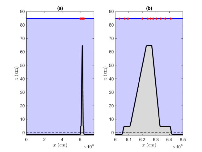
Figure 1: (a) A plot of our entire computational domain. (b) A zoomed-in plot of the “seamount.” In both plots, the horizontal line at $z\approx 84.68$ is the undisturbed water surface, the dashed horizontal line is at $z=0$, and the dots represent the gauge locations.

We numerically solve the systems given in equations (1.4), (1.10), and (1.13) using sixth-order operator splitting in time and a Fourier basis in space. The Fourier basis in space allows the linear, non-bathymetric parts of the models to be solved exactly (to within spectral resolution). This ensures that the linear phase speed of the waves is accurately reproduced. No dissipation of any sort, physical or numerical, was included in our codes. More specifically, we used no filtering to prevent numerical instabilities. We used $\tau=72.86~{}\text{cm}^{3}/\text{s}^{2}$ and $g=981~{}\text{cm}/\text{s}^{2}$ as the coefficient of surface tension and the acceleration due to gravity respectively. It is important to note that applying $\mathcal{Q}$ is a multiplication of a symmetric matrix in Fourier space. This means applying the operator $\mathcal{Q}$ is an $\mathcal{O}(M^{2}/4)$ operation. Finally, note that the inverse of $\mathcal{C}$ only needs to be computed once per simulation (not per time step) since the bathymetry does not change in time.

A drawback of using a Fourier basis is that the motion of the wave maker at the boundary cannot easily be reproduced. Therefore, we chose the initial conditions to consist of second-order Stokes waves multiplied by an envelope with compact support placed just before the seamount. The amplitude ($2$ cm), temporal period ($2.86$ sec), and wavelength ($766$ cm) of the waves were chosen to match the experimental wave parameters. Figure 2 includes a plot of the initial conditions. Since we used periodic boundary conditions and did not include dissipation, we needed to use a computational domain that was large enough that waves did not “wrap around” at the right boundary of the domain. This forced our computational domain to be much larger than the experimental tank. We used a numerical tank that with length $24000\pi$ cm. Requiring the bathymetry to have zero mean gives $h\approx 84.68$. A plot of the entire computational domain is shown in Figure 1(a).

All three systems were solved using $N=2048$ (resolution of $\eta$ and $u$ or $v$), $M=2048$ (resolution of the bathymetry), and a time step of $0.05$ seconds. For the systems given in equations (1.10) and (1.13), the conserved quantities (the integral of $\eta$, the integral of $u$ or $v$, and the Hamiltonians) were preserved to within eight or more places. Increasing the spatial or temporal resolution does not lead to a significant improvement in the preservation of the conserved quantities or a notable difference in the surface displacement predictions. This is likely due to the fact that the condition number of the matrix $\mathcal{C}$ increases from roughly 200 when $M=N=2048$ to roughly $60,000$ when $M=N=4096$ which leads to more error in computing $\mathcal{C}^{-1}$.

The Hamiltonian for the system given in equation (1.4) was preserved only to three places, while the other two conserved quantities were preserved to within 10 places. Increasing the spatial resolution to $N=M=4096$ led to numerical instabilities that destroyed the solution before the waves traveled over the entire seamount. (Recall that our code included no filtering nor dissipation.) The difficulty preserving the Hamiltonian and the numerical instabilities may be related to the possible ill-posedness of the system.

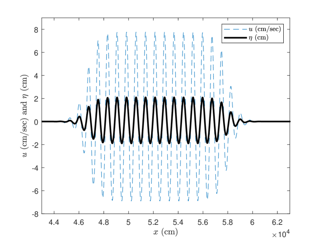
Figure 2: A zoomed-in plot of the initial conditions for the simulations. The thick solid curve represents the initial surface displacement, $\eta(x,t=0)$, and the thin dashed curve represents the initial horizontal velocity, $u(x,t=0)$. Both $\eta(x,t=0)$ and $u(x,t=0)$ are zero everywhere outside of this interval.

Figures 3, 4, and 5 include the results from the systems given in equations (1.13), (1.10), and (1.4) respectively. These plots show that system (1.4) provides the best approximation of the experimental data by far. This may be surprising because this system is thought to be ill-posed when the surface displacement is sometimes negative (as it is here). The three models provide similar predictions for the surface displacement at the first three gauges (i.e. before the bathymetry). They accurately reproduce the experimental measurements at the first three gauge locations. This suggests that all three models are accurate in the flat-bottom regime. The model predictions start to deviate at the fourth gauge and this deviation increases as the waves travel over the seamount. Setting the coefficient of surface tension to zero leads to plots that are indistinguishable to the naked eye from the plots shown. This suggests that capillarity did not play a significant role in the experiments considered here. However, it is well known that capillarity may be important in different settings (see for example [4, 31]). Regarding the nonlinear terms, we can report that predictions obtained from the linearized versions of all three models, including system (1.4), provide poor reproductions of the experimental data (plots omitted for brevity). Indeed, these considerations motivated us to aim for a versatile model which incorporates not only bathymetric effects, but also nonlinearity and capillarity.

Over the time intervals we considered, none of these systems exhibited the oscillatory instabilities found in [10, 15, 23]. Additional simulations (not shown) suggest that there may be a ratio between the amount of negative surface displacement and the length of the computational domain that determines the instability’s onset time and/or existence. It remains unclear why the accuracy of these models varies so much, though it must be said that the model which performs best by far is (1.4) which is given directly in terms of the Hamiltonian structure of the fully nonlinear water-wave problem.

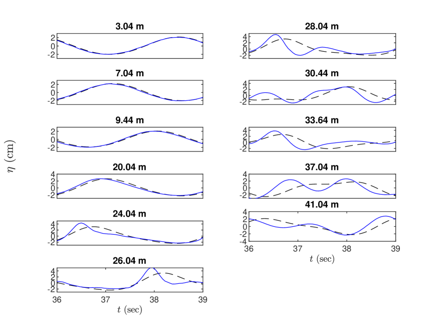
Figure 3: Plots of the experimental time series and the predictions from the system given in equation (1.13) at the eleven gauges ordered by distance from the wave maker. The solid curves are the experimental time series and the dashed curves are the model’s predictions.

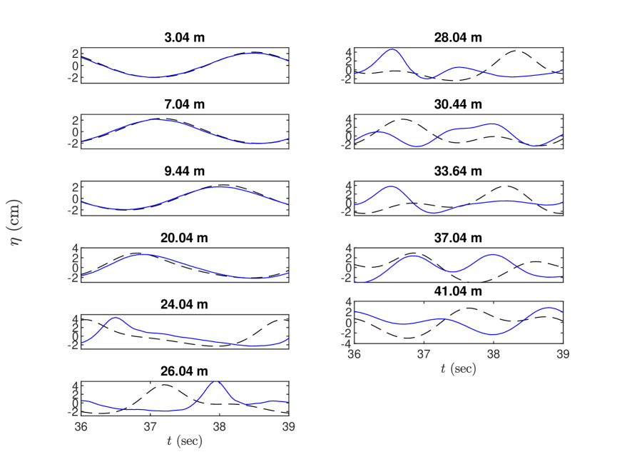
Figure 4: Plots of the experimental time series and the predictions from the system given in equation (1.10) at the eleven gauges ordered by distance from the wave maker. The solid curves are the experimental time series and the dashed curves are the model’s predictions.

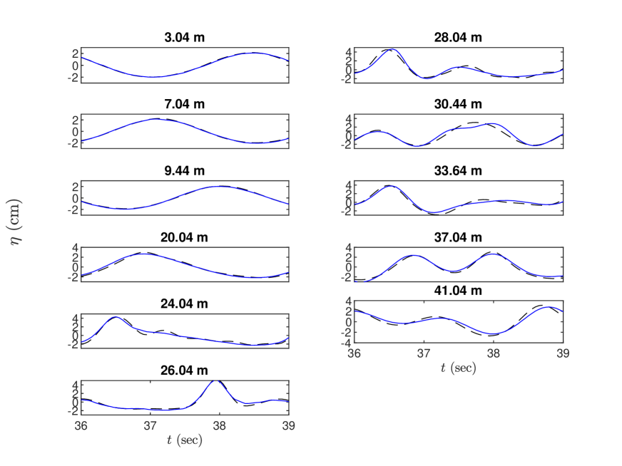
Figure 5: Plots of the experimental time series and the predictions from the system given in equation (1.4) at the eleven gauges ordered by distance from the wave maker. The solid curves are the experimental time series and the dashed curves are the model’s predictions.

For comparative purposes, we developed an alternative code using up to three of the terms in the series approximation to $L$ given in equation (4.3). These computations are faster than the computations of the full systems because the operators $L_{j}$ can be computed entirely with FFTs while applying the complete $L$ operator requires a convolution which takes $\mathcal{O}(M^{2}/4)$ operations. On the other hand, increasing the number of $L_{j}$ included in the approximation (4.3) also requires a larger number of FFTs in the computation, so three terms appear to be a reasonable compromise. Figure 6 shows that as the number of terms in the approximation of the system given in equation (1.4) increases, the results approach those shown in Figure 5. The other two models produce similar results.

To summarize, the system (1.4) which is obtained from a direct approximation of the Hamiltonian of the water-wave systems performs best of the three models tested here. The other models are also Hamiltonian, but use either different canonical variables or a different Hamiltonian structure, and this is a potential reason why the system (1.4)performs best. One might note that good agreement with the data of Dingemans has been found by other authors based on Boussinesq codes (see [9] for example). However, these higher-order models generally have many parameters which need to be tuned. On the other hand, the model proposed here needs no tuning at all.

For future work, it would be interesting to extend the systems studied here to more highly nonlinear situations. Indeed in some cases large wave heights occur due to storms, and especially near the surf zone, and in this case, Boussinesq models may cease to be applicable. For larger wave heights, it is possible to use higher-order Boussinesq or Serre-Green-Naghdi models, such as detailed in [22, 35]. In order to capture breaking waves in the surf zone, some models transition to a non-dispersive shallow-water system based on a breaking parameter, such as explained in [5, 6, 20, 34, 33]. However, so far we do not know of a system combining fully dispersive properties with a fully or even moderately nonlinear approximation.

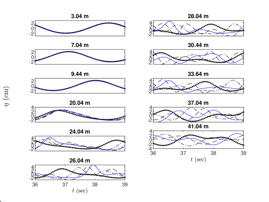
Figure 6: Plots of the experimental time series (solid curve) and the predictions from the system given in equation (1.4) using the $L_{1}$ approximation (dotted curve), $L_{1}+L_{2}$ approximation (dash dotted curve), and the $L_{1}+L_{2}+L_{3}$ approximation (dashed curve).

References

- [1] P. Aceves-Sánchez, A.A. Minzoni, and P. Panayotaros. Numerical study of a nonlocal model for water-waves with variable depth. Wave Motion, 50:80–93, 2013.
- [2] T. Alazard, N. Burq, and C. Zuily. On the water-wave equations with surface tension. Duke Mathematical Journal, 158:413–499, 2011.
- [3] D. Andrade and A. Nachbin. A three-dimensional Dirichlet-to-Neumann operator for water waves over topography. Journal of Fluid Mechanics, 845:321–345, 2018.
- [4] P.J. Aston. Local and global aspects of the (1, n) mode interaction for capillary-gravity waves. Physica D, 52:415–428, 1991.
- [5] P. Bacigaluppi, M. Ricchiuto, and P. Bonneton. Implementation and evaluation of breaking detection criteria for a hybrid Boussinesq model. Water Waves, 2:207–241, 2020.
- [6] M. Bjørkavåg and H. Kalisch. Wave breaking in Boussinesq models for undular bores. Physics Letters A, 375:1570–1578, 2011.
- [7] M. Brocchini. A reasoned overview on Boussinesq-type models: the interplay between physics. Proceedings of the Royal Society of London Series A, 469:1–27, 2013.
- [8] J.D. Carter. Bidirectional Whitham equations as models of waves on shallow water. Wave Motion, 82:51–61, 2018.
- [9] F. Chazel, D. Lannes, and F. Marche. Numerical simulations of strongly nonlinear and dispersive waves using a Green-Naghdi model. Journal of Scientific Computing, 48:105–116, 2011.
- [10] K.M. Claassen and M.A. Johnson. Numerical bifurcation and spectral stability of wavetrains in bidirectional Whitham models. Studies in Applied Mathematics, 141:205–246, 2018.
- [11] W. Craig and M.D. Groves. Hamiltonian long-wave approximations to the water-wave problem. Wave Motion, 19:367–389, 1994.
- [12] W. Craig, P. Guyenne, D.P. Nicholls, and C. Sulem. Hamiltonian long-wave expansions for water waves over a rough bottom. Proceedings of the Royal Society of London Series A, 461:839–873, 2005.
- [13] M.W. Dingemans. Comparison of computations with Boussinesq-like models and laboratory measurements. Delft Hydraulics memo H1684.12, 1994.
- [14] E. Dinvay. On well-posedness of a dispersive system of the Whitham-Boussinesq type. Applied Mathematics Letters, 88:13–20, 2019.
- [15] E. Dinvay, D. Dutykh, and H. Kalisch. A comparative study of bi-directional Whitham systems. Applied Numerical Mathematics, 141:248–262, 2019.
- [16] E. Dinvay and D. Nilsson. Solitary wave solutions of a Whitham-Boussinesq system. arXiv:1902.09438, 2019.
- [17] E. Dinvay, S. Selberg, and A. Tesfahun. Well-posedness for a dispersive system of the Whitham-Boussinesq type. SIAM Journal on Mathematical Analysis, 52:2353–2382, 2020.
- [18] M.F. Gobbi and J.T. Kirby. Wave evolution over submerged sills: tests of a high-order Boussinesq model. Coastal Engineering, 37:57–96, 1999.
- [19] V.M. Hur and A.K. Pandey. Modulational instability in a full-dispersion shallow water model. Studies in Applied Mathematics, 142:3–47, 2019.
- [20] M. Kazolea, A. Delis, and C. Synolakis. Numerical treatment of wave breaking on unstructured finite volume approximations for extended Boussinesq-type equations. Journal of Computational Physics, 271:281–305, 2014.
- [21] D. Lannes. The Water Waves Problem. American Mathematical Society, Providence, RI, 2013.
- [22] D. Lannes and P. Bonneton. Derivation of asymptotic two-dimensional time-dependent equations for surface water wave propagation. Physics of Fluids, 21:016601, 2009.
- [23] P.A. Madsen and D.R. Fuhrman. Trough instabilities in Boussinesq formulations for water waves. Journal of Fluid Mechanics, 889:A38, 2020.
- [24] P.A. Madsen, D.R. Fuhrman, and O.R. Sørensen. A new form of the Boussinesq equations with improved linear dispersion characteristics. Coastal Engineering, 15:371–388, 1991.
- [25] P.A. Madsen, D.R. Fuhrman, and B. Wang. A Boussinesq-type method for fully nonlinear waves interacting with rapidly varying bathymetry. Coastal Engineering, 53:487–504, 2006.
- [26] P.A. Madsen and O.R. Sørensen. A new form of the Boussinesq equations with improved linear dispersion characteristics. Part 2. A slowly-varying bathymetry. Coastal Engineering, 18:183–204, 1992.
- [27] D. Moldabayev, H. Kalisch, and D. Dutykh. The Whitham equation as a model for surface water waves. Physica D, 309:99–107, 2015.
- [28] O. Nwogu. Alternative form of Boussinesq equations for nearshore wave propagation. Journal of Waterway, Port, Coastal and Ocean Engineering, 119:618–638, 1993.
- [29] C.E. Papoutsellis. Numerical simulation of non-linear water waves over variable bathymetry. Procedia Computer Science, 66:174–183, 2015.
- [30] L. Pei and Y. Wang. A note on well-posedness of bidirectional Whitham equation. Applied Mathematics Letters, 98:215–223, 2019.
- [31] F. Remonato and H. Kalisch. Numerical bifurcation for the capillary Whitham equation. Physica D, 343:51–62, 2017.
- [32] V. Roeber, K.F. Cheung, and M.H. Kobayashi. Shock-capturing Boussinesq-type model for nearshore wave processes. Coastal Engineering, 57:407–433, 2010.
- [33] M. Tissier, P. Bonneton, F. Marche, F. Chazel, and D. Lannes. A new approach to handle wave breaking in fully non-linear Boussinesq models. Coastal Engineering, 67:54–66, 2012.
- [34] M. Tonelli and M. Petti. Simulation of wave breaking over complex bathymetries by a Boussinesq model. Journal of Hydraulic Research, 49:473–486, 2011.
- [35] G. Wei, J.T. Kirby, S.T. Grilli, and R. Subramanya. A fully nonlinear Boussinesq model for surface waves. Part 1. Highly nonlinear unsteady waves. Journal of Fluid Mechanics, 294:71–92, 1995.
- [36] G.B. Whitham. Linear and nonlinear waves. John Wiley & Sons, New York, NY, 1974.
- [37] J.M. Witting. A unified model for the evolution of nonlinear water waves. Journal of Computational Physics, 56:203–236, 1984.
- [38] V. Zakharov. Weakly nonlinear waves on the surface of an ideal finite depth fluid. American Mathematical Society Translations, 182:167–197, 1998.