Knowledge Distillation for Revenue Optimization:
Interpretable Personalized Pricing
Supplementary Material

1 A Toy Example

We use the following example to highlight the potential pitfall of a naive application of the student-teacher framework in the prescriptive setting.

Consider a market with an equal number of Type A and Type B customers, characterized by $x_{A}$ and $x_{B}$ respectively. Their demand or the response function $f(x,p)$ is shown in Figure 1. For Type A customers, $f(x_{A},p)=1$ when $p\leq 10$, 0 otherwise; similarly for Type B customers, $f(x_{B},p)=1$ when $p\leq 12$. This is known as the perfectly inelastic demand, where demand is not influenced by a change in price (up to a maximum price).

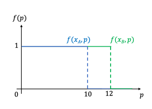
Figure 1: Response function for the toy example

With a perfect teacher model, the revenue-maximizing price for Type A and B customers are simply their respective maximum valuation, i.e., $p^{*}_{A}=10$ and $p^{*}_{B}=12$, and the optimal expected revenue is $\mathcal{R}^{*}=\frac{1}{2}(10)+\frac{1}{2}(12)=11$.

Suppose only a single price is allowed. One way of naively applying the student-teacher framework here is to use a regression tree with a single leaf to approximate the optimal prices given by the teacher model by minimizing Mean Square Error, from which we obtain $p_{RT}=\frac{1}{2}(p^{*}_{A}+p^{*}_{B})=11$ and $\mathcal{R}_{RT}=\frac{11}{2}$. On the other hand, with the student prescriptive tree whose objective is to maximize revenue, its price and revenue are given by $p_{SPT}=10$ and $\mathcal{R}_{SPT}=10$ respectively. The difference in terms of the revenue between the two methods is given by $\mathcal{R}_{RT}=\frac{11}{20}\mathcal{R}_{SPT}$. More generally, with inelastic demand given in this setup, as the maximum valuations between the two types of customers diminish, the revenue generated by the regression tree reduces to 50% of what is achievable with the prescriptive student tree.

2 Proof of Theorem 1

We begin by partitioning the feature space $[0,1]^{d}$ into a set of hypercubes of width $\frac{1}{m}$, where $m\in\mathbb{Z}^{+}$. Note, the furthest euclidean distance between any two points in each hypercube is $\frac{\sqrt{d}}{m}$.

An axis aligned binary tree of depth $k\in\mathbb{Z}^{+}$ is able to partition the feature space into any set of $2^{k}$ hyperrectangles. In particular find $\tilde{k}=\max k\in\mathbb{Z}^{+}$ such that $2^{k}\leq m^{d}$. Then $m^{-1}\leq 2^{\frac{-\tilde{k}}{d}}$.

Denote $S(x)$ as subset of observations which are in the same hypercube as $x$. For notational convenience, let $p^{*}=\tau^{*}(x)$ and $\hat{p}=\operatorname*{\rm argmax}_{p}\sum_{i\in S(x)}p\hat{f}(x_{i},p)$ be an estimation of the revenue maximizing price for hypercube which contains $x$. This is a feasible tree policy for a depth of $\tilde{k}$. The regret can be bounded as follows:

$$\tau^{*}(x) f(x,\tau^{*}(x))-\hat{\tau}(x)f(x,\hat{\tau}(x))$$

$$=p^{*}f(x,p^{*})-\hat{p}f(x,\hat{p})$$

$$=p^{*}f(x,p^{*})-\frac{1}{|S(x)|}\sum_{i\in S(x)}\hat{p}\hat{f}(x_{i},\hat{p})+\frac{1}{|S(x)|}\sum_{i\in S(x)}\hat{p}\hat{f}(x_{i},\hat{p})-\hat{p}f(x,\hat{p})$$

$$\leq p^{*}f(x,p^{*})-\frac{1}{|S(x)|}\sum_{i\in S(x)}p^{*}\hat{f}(x_{i},p^{*})+\frac{1}{|S(x)|}\sum_{i\in S(x)}\hat{p}\hat{f}(x_{i},\hat{p})-\hat{p}f(x,\hat{p})$$

$$\leq p^{*}f(x,p^{*})-\frac{1}{|S(x)|}\sum_{i\in S(x)}p^{*}f(x_{i},p^{*})+\mathcal{K}(n)$$

$$\qquad\qquad\qquad\qquad+\frac{1}{|S(x)|}\sum_{i\in S(x)}\hat{p}f(x_{i},\hat{p})-\hat{p}f(x,\hat{p})+\mathcal{K}(n)$$

$$=\frac{1}{|S(x)|}\sum_{i\in S(x)}\left[p^{*}f(x,p^{*})-p^{*}f(x_{i},p^{*})\right]+$$

$$\qquad\qquad\qquad\qquad\frac{1}{|S(x)|}\sum_{i\in S(x)}\left[\hat{p}f(x_{i},\hat{p})-\hat{p}f(x,\hat{p})\right]+2\mathcal{K}(n)$$

$$\leq\frac{1}{|S(x)|}\sum_{i\in S(x)}L|x_{i}-x|+\frac{1}{|S(x)|}\sum_{i\in S(x)}L|x_{i}-x|+2\mathcal{K}(n)$$

$$\leq L\frac{\sqrt{d}}{m}+L\frac{\sqrt{d}}{m}+2\mathcal{K}(n)$$

$$\leq 2L\sqrt{d}2^{\frac{-\tilde{k}}{d}}+2\mathcal{K}(n)$$

$$=2^{\frac{-\tilde{k}}{d}+1}L\sqrt{d}+2\mathcal{K}(n)$$

The third inequality follows from optimality of $\hat{p}$ over the estimated revenue for the observations which fall in that leaf. The fourth inequality follows from the uniform bounds on the estimation error and triangle inequality. The fifth inequality follows from the Lipschitz continuity assumption and the sixth inequality follows from the maximum distance between two points in each hypercube. The final equality is due to the ability of a binary tree of depth $\tilde{k}$ to replicate the hypercubes of width $\frac{1}{m}$.

3 Synthetic experiments

Datasets (1)-(6) used are visualized in Figure 2. This provides insight into the shape of expected revenue, as a function of the treatment (price), $X_{i}$ or $h(X)$ (the coefficient in front of price) depending on what illustrates the relationship most intuitively.

Figure 3 shows how the expected revenue changes as the size of the training sets changes for the methods we benchmark against.

Figure 4 shows how the expected revenue changes as the depth of the tree changes for the methods we benchmark against.

Remarks on an alternative implementation of distillation Another approach which uses the idea from knowledge distillation is as follows, train a teacher model that learns demand, then train a student model to approximate the teacher, and lastly optimize based on the student model. We implemented the approach on Dataset (4), and revenue obtained as tree depth increases from 1 to 10 is: 1.85, 1.84, 2.44, 2.58, 2.80, 2.98, 3.02, 3.05, 3.03, 3.04 (averaged over 10 repetitions). We observe this approach is significantly worse than the prescriptive methods we benchmark against comparing for the same depth tree (see fig 2a in paper with same experimental set-up). It appears this method needs a much greater depth (therefore impacting interpretabilty) to start achieving sensible results. However, even at depth 10, the results are inferior to even very shallow SPT trees (i.e. SPT achieves 3.4 revenue at depth 3 in Fig 2a in the main paper). Other datasets resulted in similar performance. We conjecture that a significant difference is that SPT finds splits which result in homogeneity of optimal price, whereas this approach finds splits which find homogeneity in predicted outcome.

4 Preprocessing on Dunnhumby data

The original data is in a format where each row corresponds to an item purchased on a shopping trip. To make personalized prediction on whether an item would be purchased on a particular trip by a given shopper, the data was transformed to a format where each row corresponds a shopping trip, and a label was assigned to indicate whether the item was purchased. However, when an item is not purchased in a particular shopping trip, it’s price is not recorded. Due to observed differences in the price trends over time, different imputation approaches are used for strawberries and milk. For strawberries, the price was assumed to be the mode of the price of the previous 3 sales. This is consistent with the slow moving price trends observed for strawberries where the price changed infrequently. There did not appear to be differences in pricing on a store to store level. This imputation approach has an accuracy of 83% and is marginally more accurate than just using the previous price 80%. Milk on the other hand, had significant variability in the price between stores. To impute the price for milk, we used the price of the last milk sale at that store. Only stores with at least 50 sales of milk were included in the data, to avoid long time lags between purchases. This imputation approach has an accuracy of 77% accuracy with last observation of the store, compared to 49% using the last purchased price without conditioning on the store.

The price for strawberries follows a discrete ladder of prices (from $1.99 to $4.99 per unit in $0.50 increments). The price for milk gallons follows a more irregular discrete ladder of prices, with 90% of prices falling in the set $\{\$1.66,\$1.99,\$2.32,\$2.49,\$2.69,\$2.79,\$2.89\}$, with $\$2.32,\$2.49,\$2.69$ being the most popular prices. The personalized prices in the algorithms are restricted to the same discretization. The processed data was also restricted to shoppers who purchased strawberries or milk at least once over the 2 years studied. For strawberries, this results in a dataset with 102080 shopping trips, with 3373 instances where strawberries are purchased, while milk has 89936 trips with 7688 purchases.

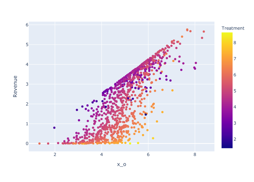
(a) Dataset 1

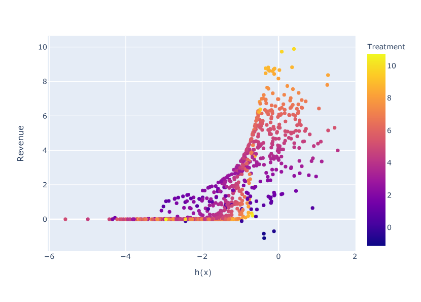
(b) Dataset 2

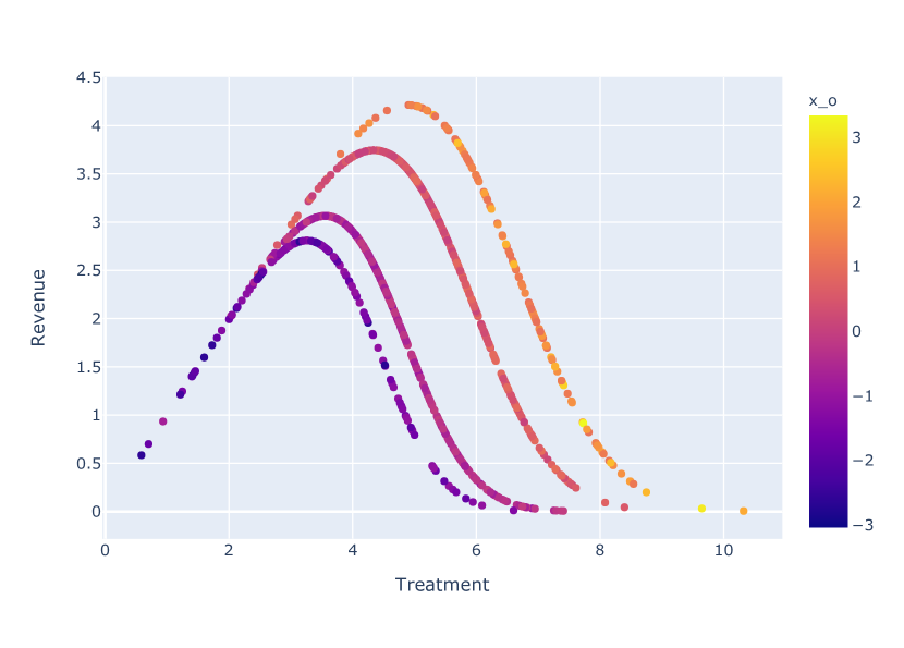
(c) Dataset 3

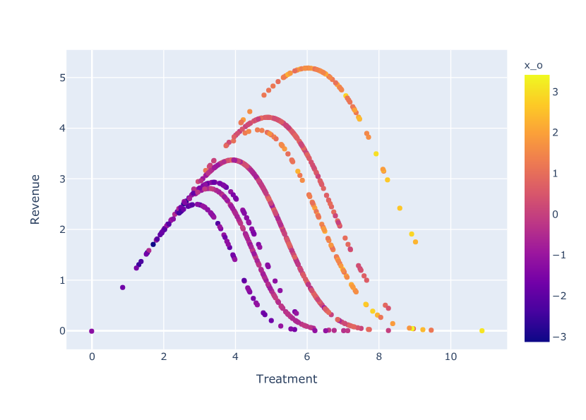
(d) Dataset 4

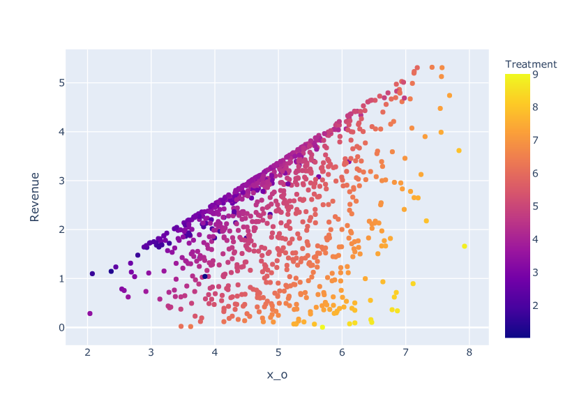
(e) Dataset 5

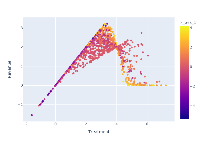
(f) Dataset 6

Figure 2: Visualization of revenue of synthetic datasets

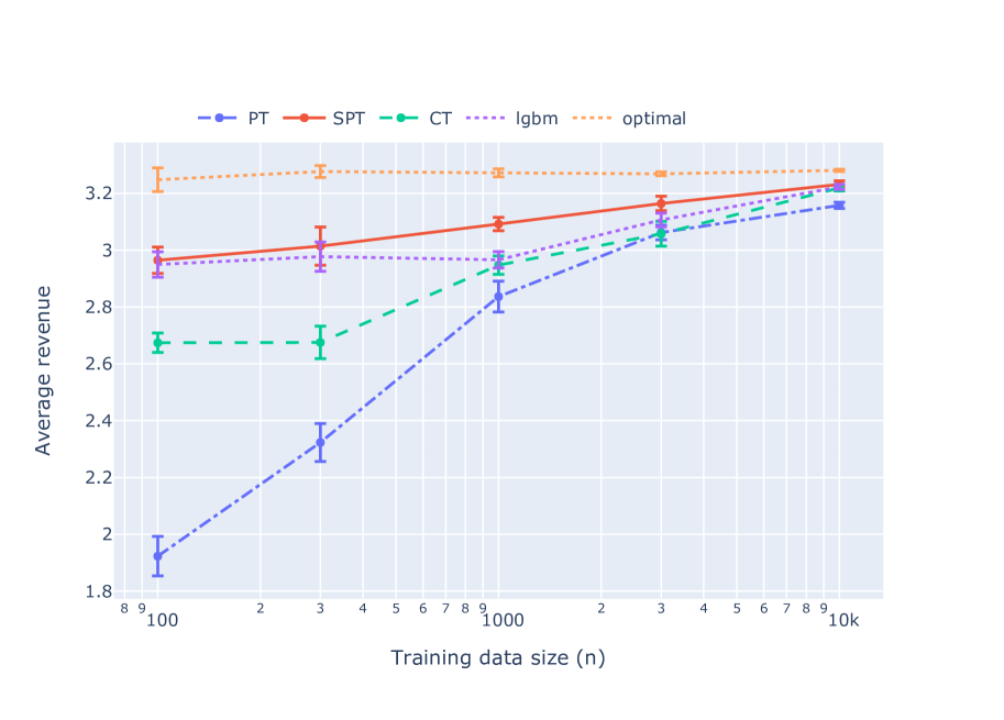
(a) Dataset 1

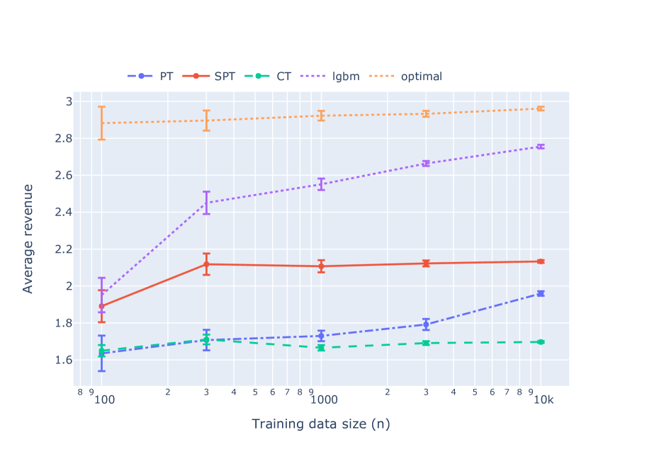
(b) Dataset 2

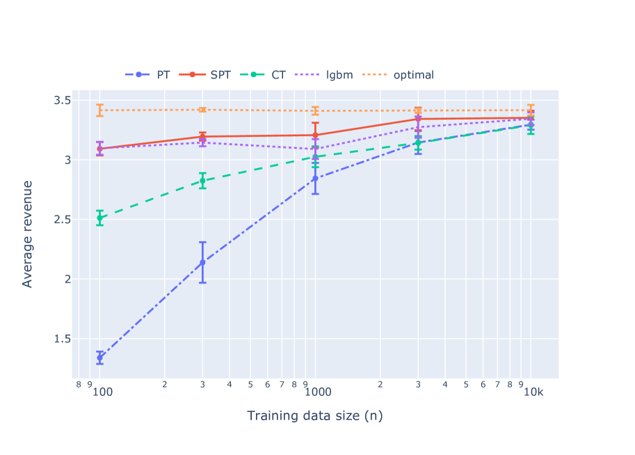
(c) Dataset 3

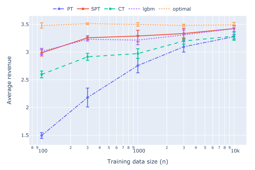
(d) Dataset 4

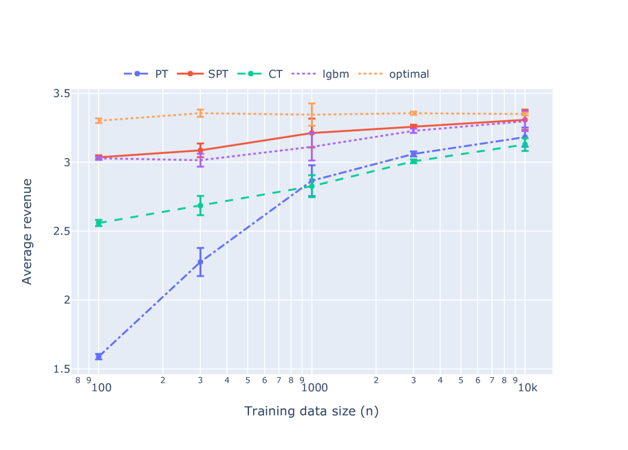
(e) Dataset 5

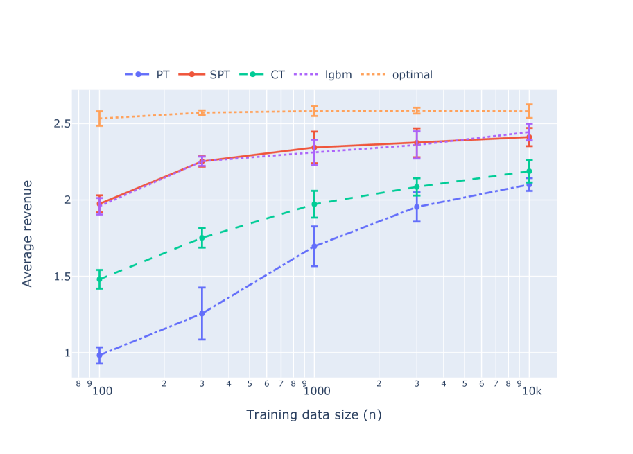
(f) Dataset 6

Figure 3: Experiments synthetic data with with increasing data (n)

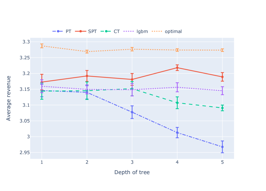
(a) Dataset 1

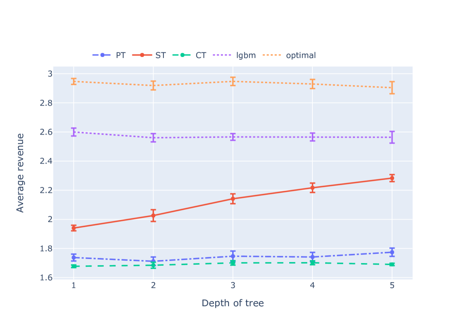
(b) Dataset 2

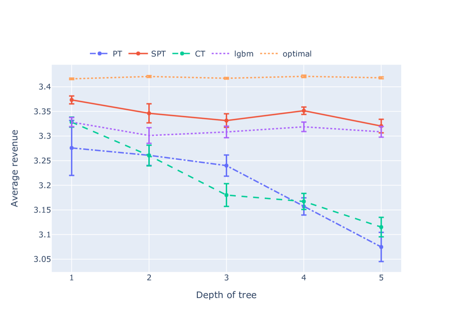
(c) Dataset 3

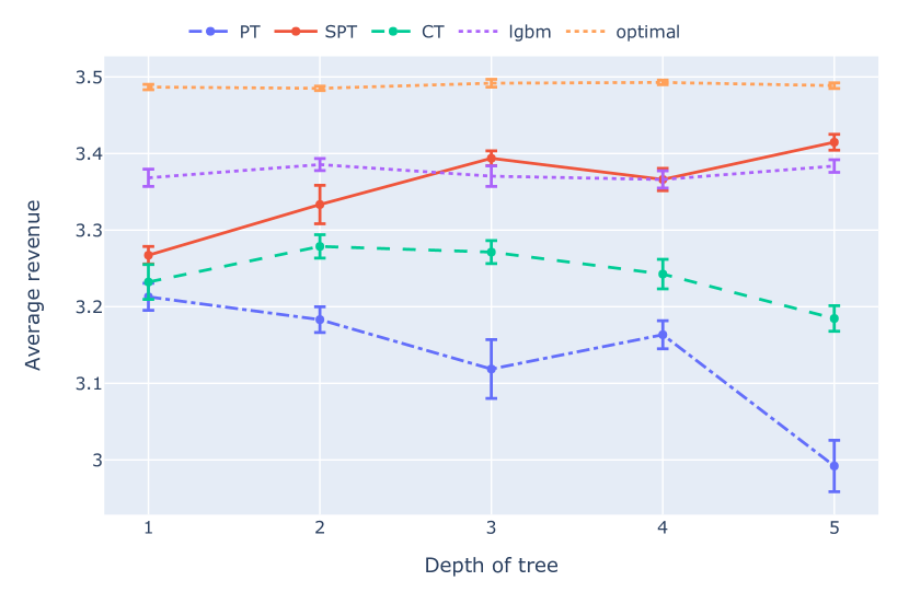
(d) Dataset 4

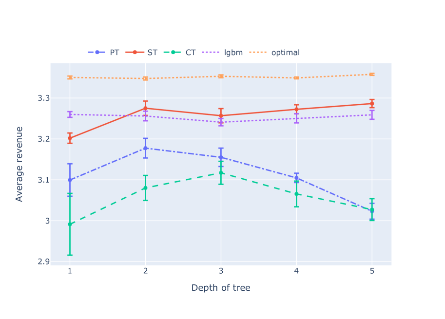
(e) Dataset 5

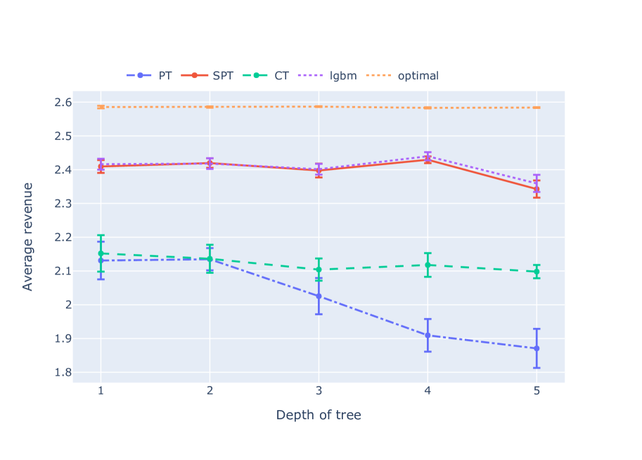
(f) Dataset 6

Figure 4: Experiments synthetic data with increasing tree depth