Hi intensity mapping with MeerKAT: 1/f noise analysis

Abstract

The nature of the time correlated noise component (the 1/f noise) of single dish radio telescopes is critical to the detectability of the HI signal in intensity mapping experiments. In this paper, we present the 1/f noise properties of the MeerKAT receiver system using South Celestial Pole (SCP) tracking data. We estimate both the temporal power spectrum density and the 2D power spectrum density for each of the antennas and polarizations. We apply Singular Value Decomposition (SVD) to the dataset and show that, by removing the strongest components, the 1/f noise can be drastically reduced, indicating that it is highly correlated in frequency. Without SVD mode subtraction, the knee frequency over a $20\,$MHz integration is higher than $0.1\,\rm Hz$; with just $2$ mode subtraction, the knee frequency is reduced to $\sim 3\times 10^{-3}\,{\rm Hz}$, indicating that the system induced 1/f-type variations are well under the thermal noise fluctuations over a few hundred seconds time scales. The 2D power spectrum shows that the 1/f-type variations are restricted to a small region in the time-frequency space, either with long wavelength correlations in frequency or in time. This gives a wide range of cosmological scales where the 21cm signal can be measured without further need to calibrate the gain time fluctuations. Finally, we demonstrate that a simple power spectrum parameterization is sufficient to describe the data and provide fitting parameters for both the 1D and 2D power spectrum.

1 Introduction

A major goal of modern cosmology is to understand the formation and evolution of the cosmological large-scale structure (LSS), as well as the information it carries from the early universe. In the past decades, cosmologists have traced the LSS fluctuations with wide-field spectroscopic and photometric surveys of galaxies (Cole et al., 2005; Eisenstein et al., 2005; Anderson et al., 2014; Hinton et al., 2017). However, these surveys are often limited with either cosmologically small volumes or lower sampling density. Furthermore, detecting individual objects at high significance is time consuming.

Recently, the $21{\rm cm}$ emission line of Neutral Hydrogen (Hi) hyperfine spin-flip transition, has been proposed as another cosmological probe of the LSS (e.g. Battye, Davies & Weller, 2004; McQuinn et al., 2006; Pritchard & Loeb, 2012). Instead of observing the Hi emission line from individual galaxies, cosmologists proposed to measure the total Hi intensity of the galaxies within large voxels, a technique known as Hi intensity mapping (IM) (Chang et al., 2008; Loeb & Wyithe, 2008; Mao et al., 2008; Pritchard & Loeb, 2008; Wyithe & Loeb, 2008; Wyithe, Loeb & Geil, 2008; Peterson et al., 2009; Bagla, Khandai & Datta, 2010; Seo et al., 2010; Lidz et al., 2011; Ansari et al., 2012; Battye et al., 2013). Because of the low angular resolution requirement, an Hi IM survey can be quickly carried out with single dishes and extended to very large survey volumes. The Hi IM technique was explored with the Green Bank Telescope (GBT), by measuring the cross-correlation function between an Hi IM survey and a optical galaxy survey (Chang et al., 2010). Later, the cross-correlation power spectrum between an Hi IM survey and an optical galaxy survey was also reported with the GBT and Parkes telescopes (Masui et al., 2013; Li et al., 2014; Anderson et al., 2018; Wolz et al., 2017), while the Hi IM auto power spectrum remains undetected (Switzer et al., 2013). There are several planned Hi IM experiments targeting the post-reionization epoch, such as the Tianlai project (Chen, 2012), the Canadian Hydrogen Intensity Mapping Experiment (CHIME Bandura et al. (2014)), the Baryonic Acoustic Oscillations from Integrated Neutral Gas Observations (BINGO Battye et al. (2013)) and the Hydrogen Intensity and Real-Time Analysis experiment (HIRAX Newburgh et al. (2016)). The SKA has also been proposed as a major instrument to probe cosmology using this technique (Santos et al., 2015; Bull et al., 2015; Square Kilometre Array Cosmology Science Working Group et al., 2020). Recently, it was also proposed to have an Hi IM survey with the newly built MeerKAT telescope in single-dish mode (Santos et al., 2017).

There are several challenges for Hi IM power spectrum detection. The primary challenge is to remove the bright continuum radiation of the Milky Way and extragalactic galaxies. The continuum radiation foreground is known to have a smooth frequency spectrum and can be extracted by fitting the spectrum with low order polynomial functions (Mao, 2012). However, due to instrumental effects, the smooth-spectrum assumption breaks down and the foreground signal leaks into higher order fluctuation modes. Several foreground cleaning methods have been proposed to try to address this (Alonso, Ferreira & Santos, 2014; Wolz et al., 2015) and used in the analysis of GBT and Parkes Hi IM survey (Switzer et al., 2015; Wolz et al., 2017).

Hi IM measurements also requires the receiver system to be stable. However, the receiver system noise is known to have time correlated fluctuations, the so-called 1/f-type noise (1/f noise). Such 1/f noise injects long-range correlations in time and leads to stripes in the final IM map. Since the measurements are performed in single dish mode (auto-correlation), they do not benefit from the suppression of 1/f noise afforded by interferometric measurements. The 1/f noise effect has been discussed in previous analyses of Cosmic Microwave Background (CMB) experiments (Janssen et al., 1996). Several different destriping methods have been proposed and tested with the analysis of CMB data (Maino et al., 2002; Seiffert et al., 2002; Keihänen et al., 2004; Kurki-Suonio et al., 2009; Sutton et al., 2010).

The effect of 1/f noise on an Hi IM survey has been analysed through simulations (Bigot-Sazy et al., 2015; Harper et al., 2018). In the case of Hi IM, the data are collected across multiple frequency channels. However, the correlation of 1/f noise across frequency is currently not very well understood. In this work, we develop a 1/f noise power spectrum density estimator to extract the temporal and spectroscopic 1/f noise properties of the MeerKAT receiver system using astronomical observation data. We also apply Singular Value Decomposition (SVD) to the data in order to reduce the 1/f-type fluctuations. The paper is organized as followed. Our power spectrum density analysis method and the 1/f noise model are introduced in Sect. (2); the details of observation data are given in Sect. (3); the SVD method is introduced in Sect. (4); a mask filling method is introduced in Sect. (5) to reconstruct the missing data due to the RFI flagging; the results are discussed in Sect. (6); and the conclusions are summarized in Sect. (7).

2 1/f Noise Power Spectrum Density Model

2.1 Temporal Power Spectrum Density

The time-ordered data (in arbitrary units) as a function of time $t$ and frequency $\nu$, $d(t,\nu$), can be modeled as the input temperature, $T_{\rm in}(t,\nu)$, multiplied by the gain, $G(t,\nu)$:

$$d(t,\nu)=G(t,\nu)T_{\rm in}(t,\nu)+n(t,\nu),$$ (1)

where $n(t,\nu)$ represents the white noise term (a Gaussian variable uncorrelated in time and frequency). The input temperature can be expressed as $T_{\rm in}=\left(T_{\rm sky}+T_{\rm rx}\right)$, where $T_{\rm sky}$ is the sky temperature (convolved by the telescope primary beam) and $T_{\rm rx}$ is the receiver temperature. The gain, $G(t,\nu)$, refers to the gain of the amplifiers in the receiver. There are several sources of temporal fluctuations in Eq. (1). First, there are the usual sky fluctuations. Since in these observations the telescope is fixed and pointing at the South Celestial Pole (SCP), we should not see much variation, except as a result of point sources or our galaxy moving in and out of asymmetries in the primary beam (or rising and setting). These changes are expected to vary slowly over time. Second, we have instrumental fluctuations. There are slow gain drifts that we expect to be able to calibrate out, the intrinsic white noise fluctuations mentioned above that should average down in time and the “non-calibrated”, correlated gain fluctuations that are the focus of this paper (the 1/f noise). Note that even the long time scales gain drifts could in principle be incorporated in this correlated noise term although this is unnecessary as it can be calibrated out. The correlated noise has simple statistical properties (at least on timescales $\lesssim 1$ h) which we describe next.

We start by defining, $G(t,\nu)\equiv\bar{G}(\nu)+\delta G(t,\nu)$ and $T_{\rm in}(t,\nu)\equiv\bar{T}_{\rm in}(\nu)+\delta T_{\rm in}(t,\nu)$, where $\bar{G}(\nu)$ and $\bar{T}_{\rm in}(\nu)$ are the time averaged quantities. We subtract and divide the data by its time average, $\bar{d}(\nu)$, taking only the varying part for the rest of the analysis: $\delta_{d}(t,\nu)\equiv\frac{d(t,\nu)}{\bar{d}(\nu)}-1$. By dividing by $\bar{d}(\nu)$ we also cancel out the frequency dependence both from the sky and instrument (the part that is stable in time, e.g., the bandpass). To first order we can then write

$$\delta_{d}(t,\nu)\approx\frac{\delta T_{\rm in}(t,\nu)}{\bar{T}_{\rm in}(\nu)}+\frac{\delta G(t,\nu)}{\bar{G}(\nu)}+\frac{n(t,\nu)}{\bar{T}_{\rm in}(\nu)\bar{G}(\nu)}.$$ (2)

The first term corresponds to sky fluctuations, which should be small, while $\delta G/G$ incorporates the 1/f-type fluctuations.

We are going to assume that we can model the ”non-calibrated” instrument fluctuations through a correlated Gaussian distribution (both in time and frequency). These can be characterised by the temporal power spectrum density function, $\hat{S}^{t}(f,\nu)$, which is estimated via the Fourier transfer of $\delta_{d}(t,\nu)$ along the time axis as

$$\hat{S}^{t}(f,\nu)=\left|\sqrt{\frac{\delta t}{N_{t}}}\sum_{p=0}^{N_{t}-1}\delta_{d}(p\delta t,\nu)\exp[-2\pi ifp\delta t]\right|^{2},$$ (3)

in which, $f$ is the temporal frequency; $\delta t$ is the time resolution of the data ($t=p\delta t$) and $N_{t}$ the number of time samples.

If we only have the white noise fluctuations, we can write,

$$S^{t}(f,\nu)\equiv\left<\hat{S}^{t}(f,\nu)\right>=\frac{\delta t}{N_{t}}\sum_{p=0}^{N_{t}-1}<\delta_{d}^{2}(p\delta t,\nu)>$$ (4)

$$=\delta t\frac{\sigma_{n}^{2}}{\bar{T}_{\rm in}^{2}(\nu)\bar{G}^{2}(\nu)}=\frac{\delta t}{\bar{T}_{\rm in}^{2}(\nu)}\frac{\bar{T}_{\rm in}^{2}(\nu)}{\delta t\delta\nu}=\frac{1}{\delta\nu},$$ (5)

where $\sigma_{n}^{2}$ is the white noise variance and $\sigma_{n}^{2}/\bar{G}^{2}(\nu)=\frac{T^{2}_{\rm in}}{\delta\nu\delta t}$ for a frequency bin width of $\delta\nu$ and integration time of $\delta t$ (e.g. Wilson, Rohlfs & Hüttemeister, 2009). Please note that, since $\delta_{d}$ is normalized with the system temperature, the power spectrum density is normalized with $T_{\rm sys}^{2}$. The power spectrum in the time direction from the extra 1/f-type noise component can then be modelled as (Harper et al., 2018),

$$S^{t}_{\rm fn}(f,\nu)=\frac{1}{\delta\nu}\left(\frac{f_{k}}{f}\right)^{\alpha},$$ (6)

where $\alpha$ is the spectral index of the noise. This enforces that for large $f$ the 1/f noise power spectrum goes to zero and the overall power spectrum becomes dominated by white noise. Our model for the full temporal power spectrum density function is then,

$$S^{t}(f,\nu)=\frac{A}{\delta\nu}\left(1+\left(\frac{f_{k}}{f}\right)^{\alpha}\right),$$ (7)

where $A$ ($\sim 1$) is as a free parameter fit together with $\alpha$ and $f_{k}$.

2.2 2-Dimensional Power Spectrum Density

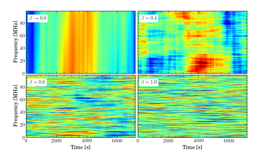
(a)

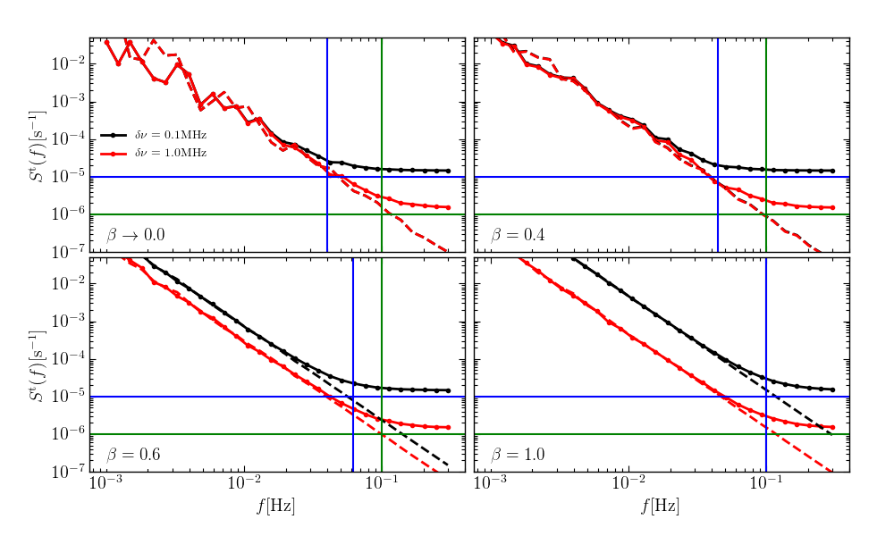
(b)

Figure 1: (a): The waterfall plot of the simulated time-ordered data using the model of Eq. (12) as the input power spectrum. The simulation uses 1/f noise parameters: $f_{k}=0.1\,{\rm Hz}$ at frequency resolution $\delta\nu=1\,{\rm MHz}$, $\alpha=2.5$ and different values of $\beta$ as shown in each panel. $\beta=1$ corresponds to uncorrelated 1/f noise across frequency while $\beta\to 0$ is fully correlated (one can still see a fluctuation since we cannot simulate $\beta=0$ exactly). (b): The temporal power spectrum density of the simulated time-ordered data as shown in Fig. (1). The black dashed curve shows the power spectrum of pure 1/f noise simulation (set white noise equals to $0$) with frequency resolution of $0.1\,{\rm MHz}$ and the solid curve shows the simulation with white noise added; The red dashed/solid curve show the same simulations with frequency resolution reduced to $1\,{\rm MHz}$. The horizontal lines indicate the white noise level with frequency resolution of $0.1\,{\rm MHz}$ (blue) and $1\,{\rm MHz}$ (green), respectively. The cross points with the vertical lines indicate the knee frequency at the corresponding frequency resolution, which is estimated with Eq. (13). For $\beta=1$ (fully uncorrelated), we expect the 1/f noise power spectrum to be inversely proportional to the frequency resolution.

The 1/f noise can potentially be correlated in frequency. We need therefore to consider a 2-dimensional power spectrum to fully describe its statistics. This 2-D power spectrum density can be estimated by Fourier transforming the observed time-ordered data along the time and frequency axes,

$$\hat{S}(f,\tau)=\left|\sqrt{\frac{\delta t\delta\nu}{N_{t}N_{\nu}}}\sum_{p=0}^{N_{t}-1}\sum_{k=0}^{N_{\nu}-1}\delta_{d}\exp\left[-2\pi i\left(fp\delta t+\tau k\delta\nu\right)\right]\right|^{2},$$ (8)

in which $f$ is the temporal frequency and $\tau$ is the spectroscopic frequency (the Fourier conjugate in the frequency domain). In this case, if we only have white noise fluctuations, $\hat{S}(f,\tau)=1$. We then build our 2-Dimensional (2D) power spectrum density model as

$$S_{\rm fn}(f,\tau)=F(f)H(\tau),$$ (9)

where $F(f)$ describes the temporal correlation power spectrum,

$$F(f)=\frac{1}{\delta\nu}\left(\frac{f_{k}}{f}\right)^{\alpha},$$ (10)

with $f_{k}$ the knee frequency defined at the frequency resolution of $\delta\nu$). $H(\tau)$ is the spectroscopic correlation power spectrum density, which can be modeled as (Harper et al., 2018),

$$H(\tau)=\left(\frac{\tau_{0}}{\tau}\right)^{\frac{1-\beta}{\beta}},$$ (11)

where $\beta$ specifies the amount of correlation across frequencies and $\tau_{0}=1/(N_{\nu}\delta\nu)$. Combining the white noise term, the 2D power spectrum model can be expressed as,

$$S(f,\tau)=A\left(1+\frac{1}{K\delta\nu}\left(\frac{f_{k}}{f}\right)^{\alpha}\left(\frac{\tau_{0}}{\tau}\right)^{\frac{1-\beta}{\beta}}\right),$$ (12)

in which, $K=\int{\rm d}\,\tau{\rm sinc}^{2}(\pi\delta\nu\tau)\left(\frac{\tau_{0}}{\tau}\right)^{(1-\beta)/\beta}$. The derivation of Eq. (12) is shown in the appendix. $A\sim 1$ due to the normalization with $T_{\rm sys}^{2}$. In our analysis, $A$ is set as an overall amplitude parameter which can be constrained by the observation data together with $f_{0}$, $\alpha$ and $\tau_{0}$.

The knee frequency $f_{k}$ as a function of frequency resolution is an important consideration for the LSS correlation signal on the largest scale sizes. For example, if we are interested in line-of-sight scales of $\sim 100\,{\rm Mpc}/h$, at $900\,{\rm MHz}$ (i.e. $z\sim 0.6$), this corresponds to frequency scales of $\sim 25\,{\rm MHz}$. Depending upon the knee frequency, at the $\sim 25\,{\rm MHz}$ frequency resolution there is the potential to detect the 1/f noise more significantly than at lower values of the frequency resolution. The knee frequency at two different frequency resolutions, $\delta\nu$, $\delta\nu^{\prime}$, is related via,

$$\lg f_{k}=\lg f_{k^{\prime}}+\frac{1}{\alpha}\lg\left(\frac{K\delta\nu}{K^{\prime}\delta\nu^{\prime}}\right).$$ (13)

The derivation is shown in the appendix. We test the shift of the knee frequency with simulated time-ordered data. Fig. (1) shows the waterfall plots of the simulated time-ordered data with different frequency correlation properties. As $\beta\to 0$, the 1/f noise becomes fully correlated over the frequency band. As $\beta\to 1$, the frequency correlation length is reduced and the 1/f noise between different frequencies becomes independent (down to the frequency resolution).

The corresponding temporal power spectrum of the simulated data is shown in Fig. (1). The black solid curve shows the power spectrum with $0.1\,{\rm MHz}$ frequency resolution, which is the raw frequency resolution of the simulation; while the red curve shows the power spectrum after averaging over $10$ frequency channels. The dashed curves show the simulation with only 1/f noise (set white noise level to 0). The horizontal lines indicate the white noise level with frequency resolution of $0.1\,{\rm MHz}$ (blue) and $1\,{\rm MHz}$ (green), respectively. The cross points with the vertical lines indicate the knee frequency at the corresponding frequency resolution, which is estimated with Eq. (13). The white noise floor, as expected, is reduced by one order of magnitude after frequency averaging. However, the 1/f noise level behaves differently with different $\beta$ values. In the case of $\beta=0$, the 1/f noise is fully correlated over the frequency band. The level of 1/f noise power spectrum does not change with averaging frequency channels, but the white noise does. The different behavior between 1/f noise and white noise results in a higher knee frequency value at lower frequency resolution. With $\beta$ increasing, the 1/f noise behaves more like the white noise. In the case of $\beta=1$, the 1/f noise if fully uncorrelated between frequencies and the power spectrum level is reduced by one order of magnitude as well. In this case, the knee frequency does not change with frequency resolution.

2.3 Parameter fitting

The parameters that characterise the 1/f noise can be constrained by fitting the model against the measured noise power spectrum. We build the $\chi^{2}$ function both for temporal and the 2-D power spectrum density function,

$$\chi^{2}_{t}=\frac{\left(\langle\hat{S}^{t}(f)\rangle_{\nu}-S^{t}(f)\right)^{2}}{\sigma^{2}_{\hat{S}^{t}}}\;\;{\rm and},\;\;\chi^{2}=\frac{\left(\hat{S}(f,\tau)-S(f,\tau)\right)^{2}}{\sigma^{2}_{\hat{S}}},$$ (14)

in which, $\langle\ \rangle_{\nu}$ represents the average over the frequency channels and $\sigma_{\hat{S}^{t}}$, $\sigma_{\hat{S}}$ are the estimated errors of the temporal and 2-D power spectrum density, respectively. The errors of the temporal power spectrum density are estimated via the standard deviation of the power spectrum density using different frequency channels,

$$\sigma^{2}_{\hat{S}^{t}}=\frac{1}{N_{\nu}}\left(\langle(\hat{S}^{t}(f))^{2}\rangle_{\nu}-(\langle\hat{S}^{t}(f)\rangle_{\nu})^{2}\right),$$ (15)

where $N_{\nu}$ is the number of frequency channels. The errors of the 2-D power spectrum density is simply estimated via,

$$\sigma^{2}_{\hat{S}}=\frac{1}{N_{\rm mode}}\hat{S}^{2}(f,\tau),$$ (16)

where $N_{\rm mode}$ is the number of Fourier modes within the $f-\tau$ bins. We constrain the free parameters by minimizing the $\chi^{2}$ function, using the publicly available Markov Chain Monte Carlo (MCMC) algorithm emcee (Foreman-Mackey et al., 2019).

3 Observations and Data Reduction

Details on the MeerKAT telescope can be found in Jonas & MeerKAT Team (2016), Camilo et al. (2018) and Mauch et al. (2020). In order to characterise the 1/f-type fluctuations of the system noise, we need a constant input signal and a long duration observation. Both requirements can be satisfied by tracking the SCP over several hours. Two SCP datasets are used in our analysis. One was collected in 2016 with a few antennas; the other was collected in 2019 using the majority of the MeerKAT array.

2016 SCP Data The data in 2016 (SCP16) was observed with three of the MeerKAT antennas, named M017, M021 and M036, pointing at the South Celestial Pole (SCP). The observation started with a $20\,{\rm Hz}$ sampling rate for $3.5\,{\rm min}$ (Experiment ID 20160922-0004), followed by $1\,{\rm Hz}$ sampling rate for $2\,{\rm hours}$ (Experiment ID 20160922-0005). The frequencies range from $856\,{\rm MHz}$ to $1711.791\,{\rm MHz}$, with $4096$ frequency channels and $0.209\,{\rm MHz}$ frequency resolution.

2019 SCP Data The SCP tracking data in 2019 (SCP19) was observed on April 24 (Experiment ID 20190424-0024) using $\sim 60$ antennas over $2.5\,{\rm hours}$. The data was taken with a $0.5\,{\rm Hz}$ sampling rate. The frequency range and resolution for the data in 2019 are the same as in 2016.

Fig. (2) shows the frequency spectrum of the SCP tracking data, averaged over the observation time. The top panel shows the spectrum of all three antennas used in the SCP16. The bottom panel shows the spectrum of the first 6 antennas used in the SCP19 observation. The amplitude shown here is the uncalibrated raw detector output power. The scattering of the amplitude across antennas is mainly due to the different digital gain settings. We use the relatively RFI-free frequency range between $1294.8672\,{\rm MHz}$ and $1503.8516\,{\rm MHz}$ for the rest of the analysis but exclude the HI signal from our galaxy at 1420MHz.

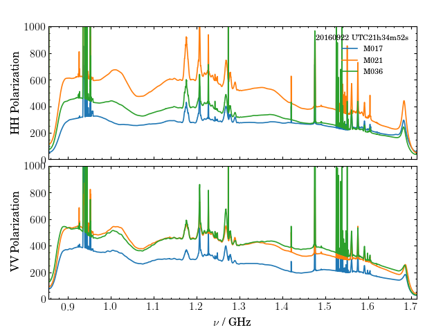
Figure 2: The frequency spectrum of SCP tracking data. The top panel shows the spectrum of the SCP16 20Hz data; the bottom panel shows the SCP19 data. In each panel, the top/bottom sub-panels show the two polarizations. The y-axis is the uncalibrated raw detector output power.

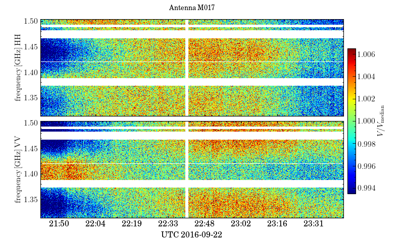
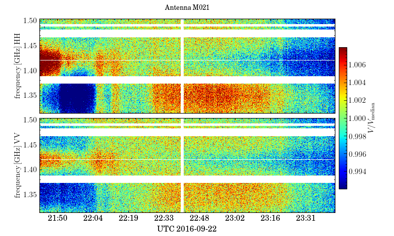
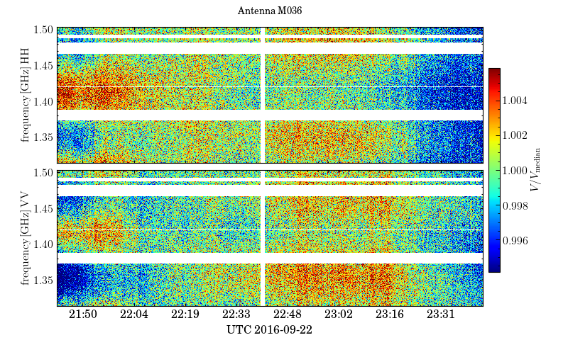
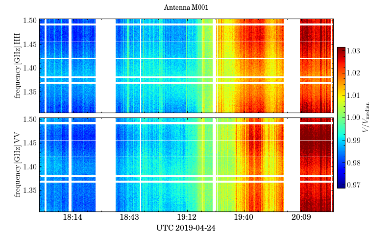
Figure 3: The waterfall plots of the SCP tracking data. The SCP16 $1\,{\rm Hz}$ data observed by antenna M017, M021 and M036 are shown in the top-left, top-right and bottom-left panels, respectively; The SCP19 data observed by M001, as an example, is shown in the bottom-right panel ($0.5\,{\rm Hz}$ sampling rate). The frequency range is truncated between $1294.8672\,{\rm MHz}$ and $1503.8516\,{\rm MHz}$, which is relatively RFI-free. The power amplitude of each frequency is normalized with the median values along the time axis. The color scale is restricted between the mean value of the shown data plus/minus $2$ times of the r.m.s. of the data.

As discussed in section 2, we are interested in the fluctuations around the time average, $\delta_{d}(t,\nu)=\frac{d(t,\nu)}{\bar{d}(\nu)}-1$. We then need to normalise the data by its time average. Note however that we use median values instead of the mean values to avoid time varying RFI. We expect the receiver temperature as well as most external sources to be constant during the observation time since the telescope is fixed and observing the SCP. Therefore, this normalisation should calibrate out the telescope bandpass as well as most spectral features from the sky, ground pick up and atmosphere. The remaining time and frequency fluctuations in $\delta_{d}(t,\nu)$ are expected to be from 1/f and white noise. However, some fluctuations can still be present from sources rising and setting and due to primary beam asymmetries. The waterfall plots of the normalized data are shown in the Fig. (3).

Three antennas from SCP16 at $1$Hz sampling rate are shown in the top-left, top-right and bottom-left panels of Fig. (3), while one antenna from SCP19, as an example, is shown in the bottom-left panel. In each panel, the two polarizations are shown in the top and bottom sub-panels. The color scale is restricted to run between the mean value plus/minus $2$ times the r.m.s. of the data shown. The amplitude varies over both frequency and observation time. The variation of SCP16 data is around $0.3\%$ of the mean, $T_{\rm sys}$, which is much less than the SCP19 data. The SCP19 data shows strong variations in time while showing strong correlations across frequency. Such frequency-correlated variations are synchronous across different antennas, which indicates an larger overall environment variation during the 2019 observation.

4 Time-ordered SVD

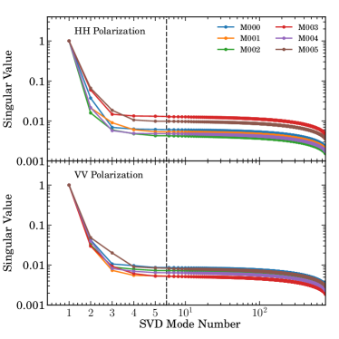
Figure 4: The singular values of each of the SVD modes, normalized to the first singular value. The black dashed line indicates the first 5 singular values. The left panel shows the singular values of the SCP16 data, both for $1\,{\rm Hz}$ and $20\,{\rm Hz}$ sampling rate, observed with different antennas. The right panels show the singular values of data from Apr. 24th, SCP19. The results of the first $6$ antennas are shown in different colors. For the $20\,{\rm Hz}$ data, the changes in amplitude are small since the modes are dominated by noise.

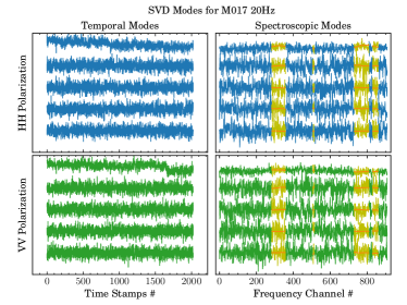
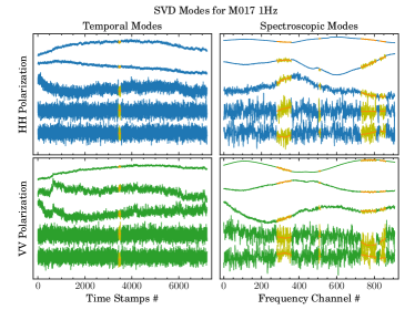
Figure 5: The singular modes of each of the first $5$ SVD modes, of antenna M017, as an example, of the SCP16 data, with results of $20\,{\rm Hz}$ data on the left panel and $1\,{\rm Hz}$ data on the right. The HH and VV polarization are shown in the top and bottom sub-panels, respectively; and the temporal and spectroscopic modes are shown in the left and right sub-panels, respectively. The areas shown in yellow are the re-filled values due to the RFI flagging, and the orange curves are the Wiener filtered smooth curves. We discuss our mask-filling strategy in Sect. (5).

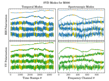
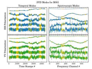
Figure 6: Same as Fig. (5) but shown with the modes of antenna M000 (left) and M001 (right) of the SCP19 data. The two polarizations are shown in the top and bottom sub-panels; and the temporal and spectroscopic modes are shown in the left and right sub-panels, respectively.

We apply Singular Value Decomposition (SVD) to the time-ordered data in order to extract its strongest components. If the 1/f noise is strongly correlated in frequency, we expect the SVD will be able to remove it while keeping the 21cm signal unaffected on the scales of interest. Foregrounds should also be removed in this process. SVD corresponds to the following matrix decomposition:

$${\bf D}={\bf U}{\bf\Lambda}{\bf V}^{\dagger},$$ (17)

where ${\bf D}$ is the data matrix with shape of $n_{t}\times n_{\nu}$; the columns of ${\bf U}=\{u_{0},...,u_{n_{t}}\}$ and ${\bf V}=\{v_{0},...,v_{n_{\nu}}\}$ are the temporal and spectroscopic modes and ${\bf\Lambda}$ is a $n_{t}\times n_{\nu}$ diagonal singular value matrix. The symbol $\dagger$ denotes the conjugate transpose. Both the temporal and spectroscopic modes are sorted according to their singular values, and the first $N_{\rm m}$ modes are subtracted,

$${\bf D}^{\rm c}={\bf D}-{\bf U}{\bf\Lambda}^{\prime}{\bf V}^{\dagger},$$ (18)

where ${\bf\Lambda}^{\prime}$ equals ${\bf\Lambda}$ with diagonals beyond $N_{\rm m}$ set to $0$. It can be further expressed as,

$${\bf D}^{\rm c} ={\bf D}-\sum_{i=0}^{N_{\rm m}}u_{i}(u_{i}^{\dagger}{\bf D})$$ (19)

$$={\bf D}-\sum_{i=0}^{N_{\rm m}}({\bf D}v_{i})v_{i}^{\dagger},$$ (20)

where $u_{i}$, $u_{i}^{\dagger}$, $v_{i}$ and $v_{i}^{\dagger}$ are the elements of ${\bf U}$, ${\bf U}^{\dagger}$, ${\bf V}$ and ${\bf V}^{\dagger}$ respectively.

The singular values of the SCP datasets are shown in Fig. (4), normalized with the first (largest) singular value. The first $5$ singular values are shown on the left of the black dashed line and the rest are shown on the right. It is clear that after the first 5 modes there is little variation in the amplitude. Therefore, we restrict the analysis in this paper to the first 5 modes. The temporal and spectroscopic modes for SCP16 and SCP19 are shown in Fig. (5) and Fig. (6), respectively. In each panel, the two polarizations are shown in the upper/lower sub-panels with blue/green colors and the temporal/spectroscopic modes shown in the left/right sub-panels, respectively. The areas shown in yellow are the re-filled values due to the RFI flagging, and the orange curves are the Wiener filtered smooth curves. We will discuss our mask-filling strategy in Sect. (5).

The $20\,{\rm Hz}$ and $1\,{\rm Hz}$ data of SCP16 have significant differences in the singular values, as well as the singular modes. The left panel of Fig. (4) shows the singular values of all three antennas of both the $20\,{\rm Hz}$ and $1\,{\rm Hz}$ data of SCP16; the singular values of the $1\,{\rm Hz}$ data decrease more quickly than those of the $20\,{\rm Hz}$ data. This is because the $20\,{\rm Hz}$ data has much shorter observation time than the $1\,{\rm Hz}$ data and the SVD modes are dominated by the system noise. This difference can also be seen with the SVD modes in Fig. (5). The two panels of Fig. (5) show the SVD modes of the antenna M017 of SCP16 data, where the $1\,{\rm Hz}$ data are on the left and the $20\,{\rm Hz}$ data are on the right. We can see that, at least for the first $3$ modes, both for the temporal and spectroscopic modes, the $1\,{\rm Hz}$ data have clear variation shapes; but the modes of $20\,{\rm Hz}$ data are mostly noise dominated.

The singular values of the data of SCP19 are shown in the right panels of Fig. (4). Only the first $6$ antennas are shown here as examples; the rest of the antennas have the same trend as these first $6$ antennas. The SVD modes of the SCP19 data are shown in the Fig. (6), in which the left and right panel show the modes of two different antennas as examples. Similar to the SCP16 $1\,{\rm Hz}$ data, with long enough observation time, the system variations both along time and frequency are well represented with the first several singular modes.

5 Power spectrum in the presence of RFI flagging

The gaps due to the RFI flagging result in significant window function effects in the final power spectrum. To reduce the impact of this effect in our analysis, we fill the missing data with values reconstructed with the SVD modes. The mask-filling strategy is described below.

First of all, some data are removed across either whole frequency channels or whole time samples. Frequency channels that are contaminated by some known narrow band RFI are fully masked for the whole observation time. The Hi emission line of the Milky Way, which is in our selected frequency band, is also removed. On the other hand, some short time duration occasional RFI, for example due to transiting satellites, are masked across the whole frequency band. By ignoring the masked frequency channels and time stamps, the rest of the data are merged into a continuous frequency-time matrix. SVD is applied to this merged data.

We take the resulting first $5$ temporal and spectroscopic modes, which have larger singular values than the noise modes, and fill the masked regions with linear interpolation. The interpolation is applied for each of the temporal and spectroscopic modes individually. However, if the singular modes are noise dominated, such as the first several modes of SCP16 $20\,{\rm Hz}$ data, the interpolation is ignored and the masked region is filled with the mean value of the singular mode. Then we apply a Wiener filter to each of the masked-filled singular modes to make the filled values smoothly connect with the unmasked region. The smoothed filling values are shown with orange curves in Fig. (5) and Fig. (6).

We then subtract the Wiener-filter-smoothed singular modes from the 5 modes, estimate the r.m.s. of the residuals for each mode and add random noise to the filling values according to the residual r.m.s. of each mode. The noise-added filling values are shown in yellow in Fig. (5) and Fig. (6). Using only these 5 modes we construct a new dataset (through Eq. (17)) which now has values in the missing gaps. We could be tempted to use these values to fill the flagged gaps in our original data. However, this reconstructed data with the first $5$ modes still has noise missing (from the remaining modes). In order to account for this, we subtract this new dataset from the original dataset and estimate an overall noise r.m.s. using the non-flagged part of the data. We then add random noise to the new dataset using this r.m.s and use its values to fill the flagged gaps in the original data. The original masked data and masked filled data of SCP19 (antenna M001) are shown in the top-left and top-right panels of Fig. (7), respectively.

Finally, we perform SVD a second time to the mask-filled data. The waterfall plots with the first $1$, $2$ and $5$ modes removed are shown in the middle-left, middle-right and bottom panels of Fig. (7). The corresponding first $5$ modes are shown in Fig. (7). The power spectrum estimation discussed in Sect. (6) is performed with the mask-filled data.

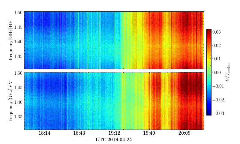
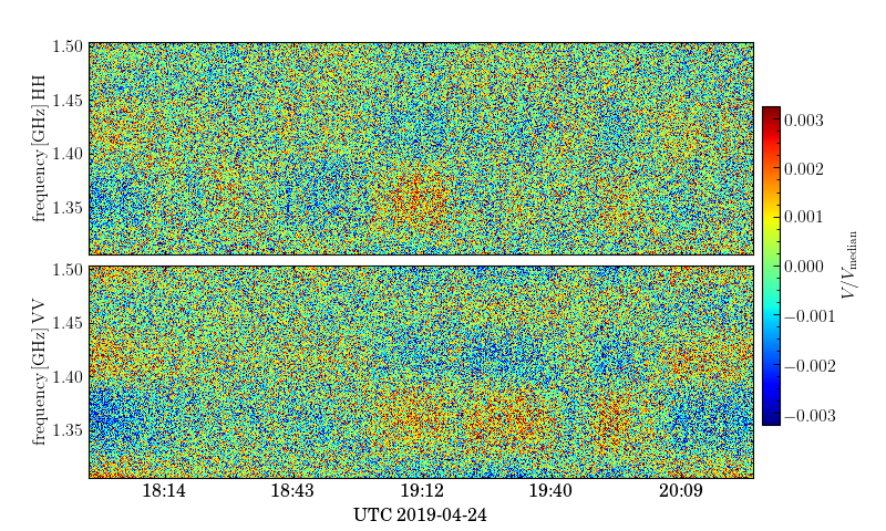
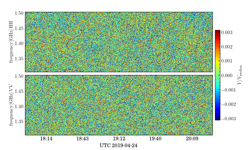
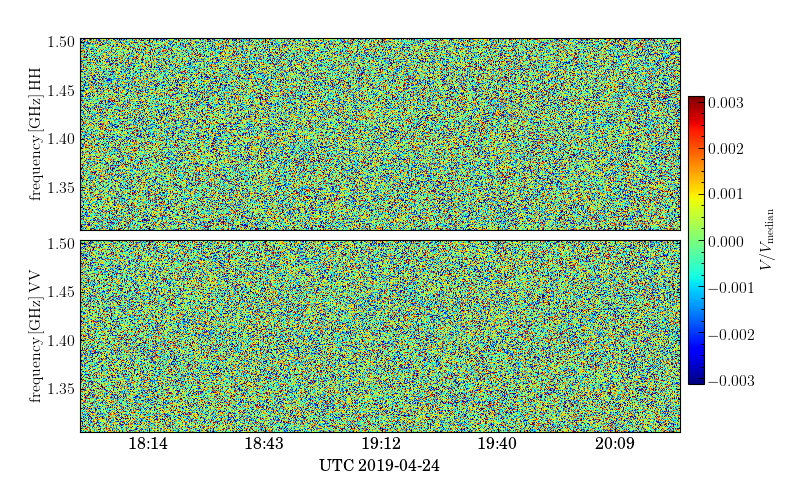
(a)

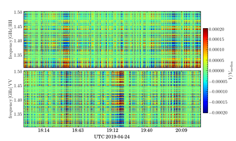
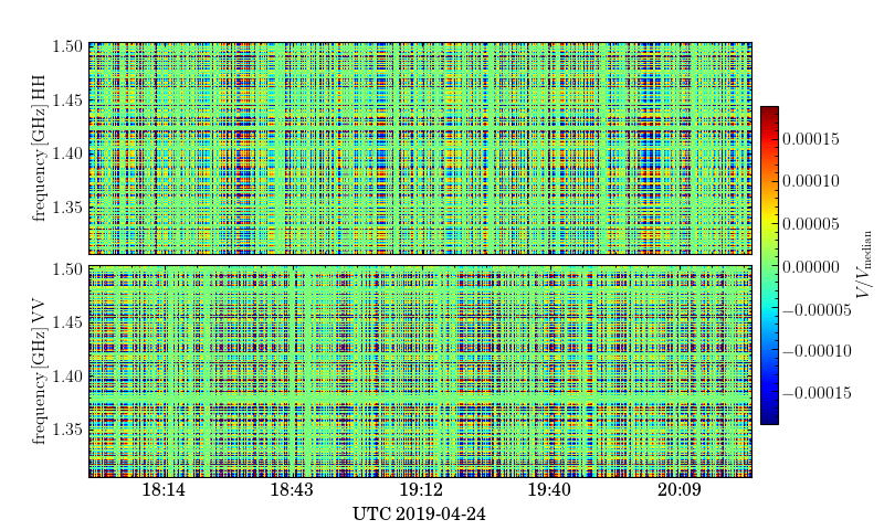
(b)

Figure 7: (a): The top-left panel shows the waterfall plots of the mean-subtracted data before SVD mode subtraction; The top-right panel shows the same data with the RFI masks filled; The middle-left, middle-right and bottom panels are the waterfall plots of the mask filled data with $1$, $2$ and $5$ SVD modes subtracted. (b): The waterfall plots of the first $5$ SVD modes from the mask filled data. All these data are the SCP19 observation with antenna M001.

6 Results and Discussion

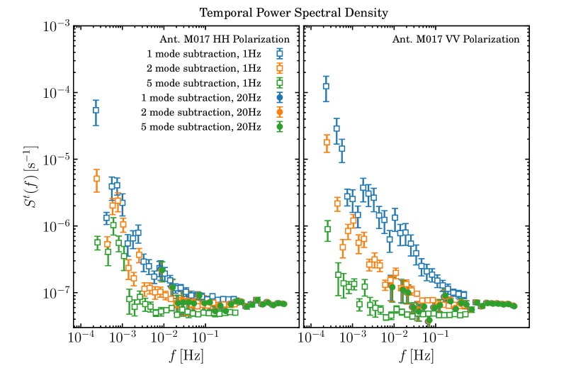
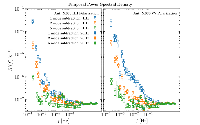
Figure 8: The temporal power spectrum density of the SCP16 data. The results of the $3$ antennas are shown in different panels. In each panel, the results of two polarizations are shown in the left and right subpanels; The results with $1$, $2$ and $5$ mode subtraction are shown in different colors as labeled in the legend. The errors of the power spectrum density are estimated via the variance over different frequency channels.

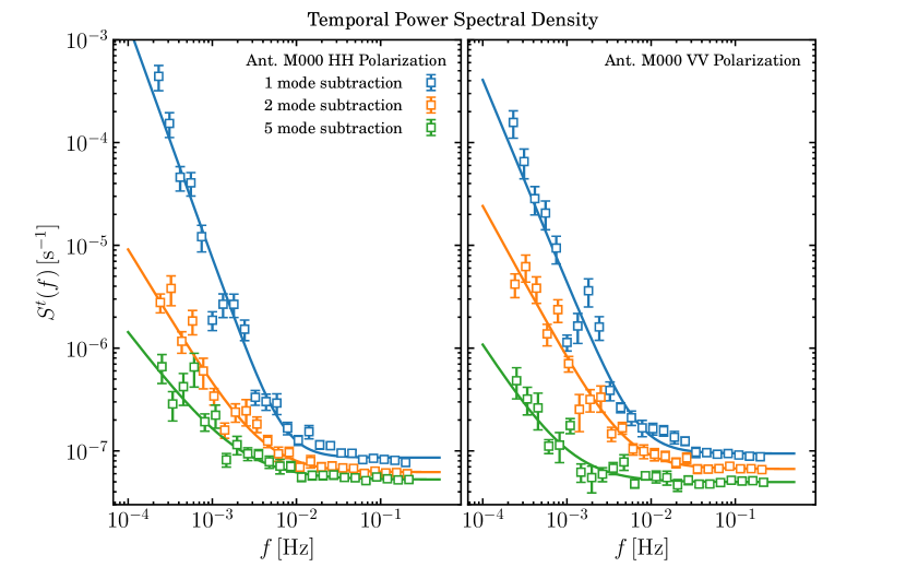
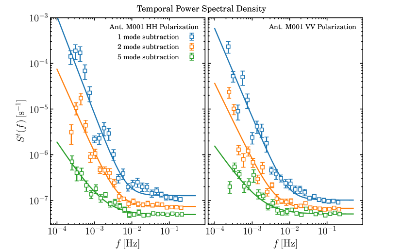
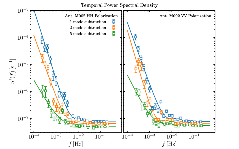
Figure 9: Same as Fig. (9) but for SCP19 datasets. The results of the first $3$ antennas are shown in different panels. The solid lines are the fitted 1/f noise temporal model using Eq. (7).

6.1 The Temporal Power Spectrum Density

We now focus on the analysis of the power spectrum along the time domain and how it compares to our model. The temporal power spectrum is estimated by Fourier transforming the data along the time axis. Before the power spectrum estimation, we reduce the frequency resolution down to $\sim 20\,{\rm MHz}$ by averaging every $100$ frequency channels. The frequency averaging can reduce the white noise level and shift the knee frequency to the high-end of $f$. However, as we discussed before, the shift of the knee frequency is also dependent on the frequency correlation of the 1/f noise.

The temporal power spectrum density results of SCP16 data observed with the three antennas are shown in Fig. (9), and the results of the first $3$ antennas of SCP19 data are shown in Fig. (9). The two polarizations are shown in the left and right subpanels. We do not show the raw data as it is mostly dominated by external sources (e.g. sky and ground pick up). This should be very smooth in frequency with our observation and most of it should be removed with the first SVD mode. The results with $1$, $2$ and $5$ mode subtraction are shown in different colors as labeled in the legend. The errors of the power spectrum density are estimated via the variance over different frequency channels. Significant 1/f-type noise in the power spectrum is visible in all the plots. After SVD modes subtraction, the 1/f-type noise power is reduced and flat white noise dominates the power spectrum over a wide frequency range, with a clear knee frequency visible. This indicates that most of the 1/f noise is correlated in frequency.

For the SCP16 data, the results with $1\,$Hz sampled data are shown with empty markers and the $20\,$Hz sampled data with filled markers. Both show good agreement of the white noise floor (Fig. (9)) . This level is also consistent with the theoretical value in Eq. (7) given by $1/\delta\nu$, which at $\delta\nu=20\,{\rm MHz}$ corresponds to $\sim 5\times 10^{-8}$. The noise floor is also slightly reduced with the $5$ modes subtraction. Note however that it is still equal or above the predicted theoretical white noise value. Mostly likely, this noise floor reduction is due to the removal of correlated modes in frequency but that are fluctuating on short time-scales.

We also notice that the SVD mode subtraction does not work well with antenna M021 for the $20\,$Hz sampled data, especially for the VV polarization. As shown in Fig. (4), the singular values of this antenna with $20\,$Hz sampled data are barely reduced. With $1\,$Hz sampled data, M021 has larger singular values for the second and third modes compared with the other two antennas. By looking at the waterfall plot in Fig. (3), M021 has more fluctuations than the other two antennas. This indicates that the system of M021 was quite unstable during the observation of SCP16.

The SVD mode subtraction works well for the SCP19 data, as shown in Fig. (9). We only show the results of the first $3$ antennas because the other antennas have similar behaviors. Comparing to SCP16 datasets, the $f$ upper bond of SCP19 is limited by the lower time sampling resolution. The solid lines in Fig. (9) are the fitted 1/f noise temporal model using Eq. (7). Again we do not fit to the raw data here as that would require a more complex model, possibly with a running power law. Once we remove one or more modes the fit using Eq. (7) works quite well. Removing two modes is quite conservative and we expect it to be done for most data analysis.

After the subtraction of the first singular mode, the 1/f type correlation in time is highly reduced and the knee frequency is reduced below $10^{-2}\,$Hz. A clear white noise floor is shown at the high-$f$ end and the noise floor is $\sim 5\times 10^{-8}$, which is consistent with both the SCP16 data, as well as the model prediction. With additional singular modes subtraction, the knee frequency is further reduced. Again, the noise floor is slightly reduced with $5$ mode subtraction.

6.2 2D Power Spectrum Density

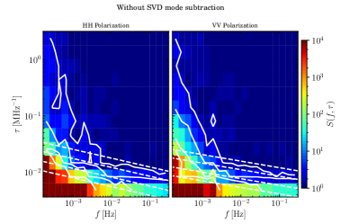
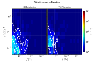
Figure 10: The 2D power spectrum density estimated with SCP19 data. From the top-left to the bottom-right, each panel shows the result with no SVD modes subtraction, one mode, two modes and five modes subtraction. The two polarization are shown in the left/right sub-panels. All the plots are truncated with the same color scale. The white contours shows the levels $2$, $10$, $10^{2}$, and $10^{3}$. and the dashed contours show the fitted power spectrum model at the same levels.

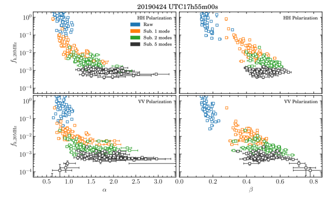
Figure 11: The fitted $f_{\rm k,20MHz}$ versus $\alpha$ (left panels) and $\beta$ (right panels) for each of the antennas. Top/bottom panels show the results of HH/VV polarizations. The results with different number of modes subtracted are shown with different colors.

Figure 12: Same as Fig. (10) but only for the results with no SVD mode subtraction (left) and five mode subtraction (right). The white dotted lines indicate the corresponding cosmological scales projecting to the $f-\tau$ space, assuming observations at $900\,{\rm MHz}$ with scanning speed of $5\ {\rm arcmin}\,s^{-1}$. $k$ is in units of ${\rm Mpc}^{-1}h$.

The 2D power spectrum density is estimated by Fourier transforming the data along both the time and frequency axes. The results for SCP19 are shown in Fig. (10) for one antenna (M000) as an example. From top-left to the bottom-right panels, it shows the 2D power spectrum with $0$, $1$, $2$ and $5$ SVD modes subtracted, as labeled in the title of each panel. The results for the two polarizations are shown in the left and right subpanels, respectively. The white contour shows the levels $2$, $10$, $10^{2}$ and $10^{3}$. The dashed contours show the fitted 2D power spectrum model at the same power spectrum levels as the measurements. Since we are analysing the power spectrum of $\delta_{d}$ (Eq. 12), the 2D power spectrum of the white noise should be at a level of $1$.

The top-left panel of Fig. (10) shows the results of the data without singular mode subtraction. The power spectrum is peaked at the low-$\tau$ end, which indicates a strong correlation across frequency channels. Such strong frequency correlation results in a smooth frequency spectrum, which is clearly shown in the waterfall plots (top panels of Fig. (7)). The power spectrum has a tail below $f\sim 10^{-2}$ extending to higher $\tau$. Such a tail structure indicates other 1/f components, which are less correlated across frequency channels. However, the model is only fitted to the component with strong frequency correlation as it is the dominant one and the model assumes a single spectrum index. This is also the reason why the temporal power spectrum model can not fit the data without singular mode subtraction as discussed in Sect. (6.1).

The strong frequency correlated component can be removed by subtracting the first singular mode. The waterfall plots of the first singular mode are shown in the top panel of Fig. (7), which have structures consistent with the raw data. The 2D power spectrum of the data with first mode subtracted is shown in the top-right panel of Fig. (10). Comparing to the top-left panel, the strong frequency correlated component is subtracted out.

With more singular modes subtraction, the 1/f-type power spectrum is highly reduced and the knee frequency is also reduced to lower values. The 2D power spectrum model, Eq. (12), is fitted to the measurements for each antenna and polarization with a differing number of SVD modes subtracted, individually. The fitting parameters $f_{\rm k,20MHz}$, $\alpha$ and $\beta$ are shown in Fig. (11), where each square marker shows the fitting value for one antenna. The results for the two polarizations are shown in the left and right panels and the results with different singular mode subtraction are shown in different colors as labeled in the legend. The median value of the fitting parameters, as well as the r.m.s, over all dishes are listed in Tab. (1).

As shown in Fig. (11), without singular mode subtraction, the fitting value for $\beta$ is less than $0.2$, which indicates a strong correlation across frequency. After one singular mode is subtracted, the $\beta$ values increase significantly, but do not keep increasing as further modes are subtracted. This indicates that the singular modes are sensitive to highly correlated structures either in frequency or time axis. The fitting value for $f_{\rm k,20MHz}$ is continuously reduced with additional singular mode subtraction. With one mode subtraction, the fitting values, especially $f_{\rm k,20MHz}$ and $\alpha$, have large scatter between different antennas. The scatter indicates that the correlation features are too complex to be described by one singular mode and the residuals, which can be different between antennas, are dominating the second singular mode. With $2$ modes subtraction, the knee frequency at $20\,$MHz is reduced to around $3\times 10^{-3}\,{\rm Hz}$, which indicates that the system 1/f-type variations are well under the thermal noise fluctuation over $\sim 3\times 10^{2}\,{\rm s}$. The time scale can be even longer with $5$ modes subtraction. However, as more modes are removed, there is the danger of over-cleaning, although $5$ or more modes removal is standard in foreground cleaning methods. We plan to investigate this behaviour further in follow up work with simulations.

Table 1: The median value of fitting parameters across all dishes. The errors are the r.m.s. of the fitting values across all dishes.

	$\lg f_{\rm k,20MHz}$		$\alpha$		$\beta$
	HH	VV	HH	VV	HH	VV
2D power spectrum density
1 mode subtraction	$-1.77\pm 0.49$	$-1.97\pm 0.38$	$0.98\pm 0.25$	$1.00\pm 0.33$	$0.42\pm 0.06$	$0.41\pm 0.06$
2 mode subtraction	$-2.49\pm 0.26$	$-2.65\pm 0.28$	$1.39\pm 0.25$	$1.39\pm 0.37$	$0.52\pm 0.05$	$0.51\pm 0.08$
5 mode subtraction	$-3.04\pm 0.13$	$-3.19\pm 0.32$	$1.70\pm 0.35$	$1.80\pm 0.55$	$0.51\pm 0.06$	$0.49\pm 0.11$
1D power spectrum density
1 mode subtraction	$-2.23\pm 0.18$	$-2.23\pm 0.18$	$2.28\pm 0.34$	$2.25\pm 0.41$	–	–
2 mode subtraction	$-2.40\pm 0.21$	$-2.40\pm 0.21$	$1.83\pm 0.40$	$1.98\pm 0.38$	–	–
5 mode subtraction	$-2.78\pm 0.14$	$-2.85\pm 0.21$	$1.28\pm 0.26$	$1.47\pm 0.37$	–	–

The white dotted lines in Fig. (12) indicate the corresponding cosmological scales projecting to the $f-\tau$ space, assuming observation at $900\,{\rm MHz}$ with scan speed of $5\,{\rm arcmin}\,s^{-1}$. The temporal and spectroscopic wavenumber, $f$ and $\tau$, are related to the cosmological scales $k$ by

$$\tau=\frac{\nu_{0}}{\nu_{\rm obs}^{2}}\frac{c}{H(z)}\frac{k_{\parallel}}{2\pi},\;\;f=\frac{k_{\perp}\chi(z)u}{2\pi},\;\;{\rm and}\;k^{2}=k^{2}_{\parallel}+k^{2}_{\perp},$$ (21)

in which, $k$ is in units of ${\rm Mpc}^{-1}h$; $\nu_{0}=1420{\rm MHz}$ is the rest frame Hi emission line frequency; $c$ is the speed of light; $\nu_{\rm obs}$ is the observing frequency and $u$ is the scanning speed. We assume the fiducial cosmology parameters from Planck Collaboration et al. (2018) ($h=0.6736$, $\Omega_{\rm m}=0.3153$ and $\Omega_{\Lambda}=0.6847$). We see that there is a large region in the $f-\tau$ space that will be available for the 21cm measurements. In particular, even without any mode subtraction, most contamination, either because of 1/f noise or foregrounds is constrained to a region of low $f$ or low $\tau$.

7 Summary and Conclusions

In this work we measured the power spectrum density of the 1/f noise for the MeerKAT receiver system. The analysis is performed with South Celestial Pole (SCP) tracking data to avoid sky variations. Two SCP tracking datasets are used in this analysis. We find a relatively RFI free frequency range from $1313.6758\,$ MHz to $1461.8457\,$ MHz. Absolute flux calibration is ignored in our analysis as the data are normalized with the time averaged system temperature for each frequency channel.

We apply Singular Value Decomposition to the data and determine how effective removing the first several principal components is on suppressing the time-frequency correlated noise. The results show that indeed, the 1/f noise can be drastically reduced by removing the first few SVD modes. Moreover, the correlation features are well described by the proposed noise model with just a few parameters. Using the parameterisation presented in Eq. (12), the removal of a single SVD mode reduces $\beta$ from $\sim 0.16$ (e.g., 1/f noise that is highly correlated in frequency) to $\beta=0.5$, which indicates a large reduction in correlation across frequency. Along the temporal axis of the time-ordered data, a similar reduction is seen, with the raw data averaged over 20 MHz having a knee frequency ($f_{k}$) of 10^-1 Hz, which is reduced to $\sim 3\times 10^{-3}\,{\rm Hz}$ with $2$ mode subtraction, indicating that the system 1/f-type variation is well under the thermal noise fluctuation over a few hundred seconds time scales. The results from this analysis, along with the described noise power spectrum model, can be used in realistic noise simulations for MeerKAT and extended to SKA1-Mid.

The 2d power spectrum shows that the 1/f noise is constrained to a small region of either low $\tau$ or low $f$, e.g. large scale correlations in time or in frequency. This provides many scales where the 21cm signal can be probed without contamination. With scanning speeds of $5\ {\rm arcmin}\,s^{-1}$, $10^{3}\,{\rm s}$ time scales would correspond to $\sim 80$ degrees, which is enough for our cosmological purposes. Longer time scales can be achieved by using noise diodes. Our calibration plan is to use celestial sources for calibration on timescales $\sim 1.5\,{\rm hour}$ (absolute flux and bandpass calibration) and noise diodes for shorter time scales. We can then apply a conservative SVD cleaning on the time-ordered data (e.g. $2$ modes) in order to remove most of the 1/f noise contamination. These modes correspond to large frequency scales where we expect the 21cm correlations to be negligible. Therefore, this cleaning should have a minor impact on the 21cm signal given what we already know about foreground cleaning methods (e.g. Alonso et al., 2015). Any residual noise will be included in the map making process which will allow for correlated noise in frequency. Finally we will apply foreground cleaning to the maps.

The 1/f noise has been a substantial challenge to precision radio cosmology in the past and, if it is not carefully treated, has been shown to be detrimental to future HI IM experiments. We have demonstrated here a methodology that can be used to effectively suppress 1/f noise in single dish HI IM observations that should preserve the cosmological signal. In future work we plan demonstrate the effectiveness of this technique both on simulated and real MeerKAT data.

Appendix A

Relation between temporal power spectrum density and 2D Power spectrum density

The temporal power spectrum density can be expressed as,

$$S_{ij}(f)=\langle\delta(f,\nu_{i})\delta^{\dagger}(f,\nu_{j})\rangle=\int{\rm d}\,\nu\,{\rm d}\,\nu^{\prime}\,\phi_{i}(\nu)\phi_{j}^{\dagger}(\nu^{\prime})\xi(f,\nu_{ij})$$ (22)

in which, $\nu_{ij}=\nu_{i}-\nu_{j}$, $\phi_{i}(\nu)$ is the spectroscopic window function and $\delta(f,\nu_{i})=\int{\rm d}\,\nu\,\phi_{i}(\nu)\delta(f,\nu)$; $\xi(f,\nu_{ij})$ is related to the 2D power spectrum density, $S(f,\tau)$, via inverse Fourier transform,

$$\xi(f,\nu_{ij})=\int{\rm d}\,\tau S(f,\tau)\exp\left[2\pi i\tau\nu_{ij}\right].$$ (23)

Substituting Eq. (23) to Eq. (22), the temporal power spectrum density can be further expressed as

$$S_{ij}(f)=\int{\rm d}\,\tau\,\phi_{i}(\tau)\phi^{\dagger}_{j}(\tau)S(f,\tau)$$ (24)

where $\phi_{i}(\tau)=\int{\rm d}\,\nu\,\phi_{i}(\nu)\exp[-2\pi i\tau\nu]$ is the Fourier transform of the spectroscopic window function. If we ignore the cross correlation between frequencies, the diagonal term of the temporal power spectrum density is,

$$S_{i}(f)=\int{\rm d}\,\tau\,\phi_{i}^{2}(\tau)S(f,\tau)$$ (25)

The white noise level

If we use a top-hat window function with width of $\delta\nu$, the Fourier transform of the top-hat window function, $\phi_{i}(\tau)$, can be expressed with a sinc function,

$$\phi_{i}(\tau)={\rm sinc}(\pi\delta\nu\tau),$$ (26)

where the window function is normalized with $\int{\rm d}\,\tau\phi_{i}^{2}(\tau)=\int{\rm d}\,\tau\phi_{i}(\tau)=1/\delta\nu$. Substituting the 2D white noise power spectrum model (the first term of Eq. (12)), Eq. (25) becomes,

$$A\int{\rm d}\,\tau\,\phi_{i}^{2}(\tau)=\frac{A}{\delta\nu},$$ (27)

which is consistent with the white noise term of 1D power spectrum density model Eq. (7).

The knee frequency conversion between frequency resolutions

We firstly model the 2D 1/f noise power spectrum density with $f_{0}$ at arbitrary frequency resolution,

$$S(f,\tau)=A\left(\frac{f_{0}}{f}\right)^{\alpha}\left(\frac{\tau_{0}}{\tau}\right)^{\frac{1-\beta}{\beta}}.$$ (28)

Substituting the noise model into Eq. (25),

$$A\left(\frac{f_{0}}{f}\right)^{\alpha}\int{\rm d}\,\tau\phi_{i}^{2}(\tau)\left(\frac{\tau_{0}}{\tau}\right)^{\frac{1-\beta}{\beta}}=AK\left(\frac{f_{0}}{f}\right)^{\alpha}$$ (29)

where $K$ is

$$K=\int{\rm d}\,\tau\,{\rm sinc}^{2}(\pi\delta\nu\tau)\left(\frac{\tau_{0}}{\tau}\right)^{\frac{1-\beta}{\beta}}.$$ (30)

The 1D power spectrum model assumes the 1/f noise is reduced with factor of $\delta\nu$, which indicates that the 1/f noise is uncorrelated across frequencies. That equivalent to set $\beta=1$ in the 2D power spectrum density model,

$$AK\left(\frac{f_{0}}{f}\right)^{\alpha} =A\left(\frac{f_{0}}{f}\right)^{\alpha}\int{\rm d}\,\tau\,{\rm sinc}^{2}(\pi\delta\nu\tau)\left(\frac{\tau_{0}}{\tau}\right)^{0}=\frac{A}{\delta\nu}\left(\frac{f_{0}}{f}\right)^{\alpha}.$$ (31)

Comparing with the second term of 1D power spectrum density model Eq. (7), we have $f_{0}=f_{k}$. This indicates that, if the 1/f noise is fully uncorrelated across frequencies, the knee frequency is constant with any frequency resolution.

On the other hand, if $\beta\to 0$, the spectroscopic spectrum density index is approaching to $+\infty$ and the spectroscopic power spectrum density model becomes a Dirac delta function, $H(\tau)\to\delta^{\rm D}(\tau)$. In this case, we have

$$AK\left(\frac{f_{0}}{f}\right)^{\alpha} =A\left(\frac{f_{0}}{f}\right)^{\alpha}\int{\rm d}\,\tau\,{\rm sinc}^{2}(\pi\delta\nu\tau)\delta^{\rm D}(\tau)=\frac{A}{\Delta\nu}\left(\frac{f_{0}}{f}\right)^{\alpha}.$$ (32)

where $\Delta\nu=1/\tau$. When $\tau=0$, $\Delta\nu\to+\infty$, indicating the infinity frequency bandwidth.

However, the measurements are always limited within finite frequency bandwidth. If we write the integrals in terms of discrete sums, Eq. (25) is expressed as,

$$S_{i}(f)=\sum_{p=0}^{N_{\nu}-1}\phi_{i}^{2}(p\tau_{0})S(f,p\tau_{0})\tau_{0},$$ (33)

where $\tau_{0}$ is the minimal spectroscopic frequency interval and related to the minimal frequency interval $\nu_{0}$ via $\tau_{0}=1/(N_{\nu}\nu_{0})=1/\Delta\nu$, where $\Delta\nu$ is the full frequency bandwidth. The Eq. (32) becomes,

$$A\left(\sum_{p=0}^{N_{\nu}-1}{\rm sinc}^{2}(\pi\delta\nu p\tau_{0})\tau_{0}\delta^{D}_{p}\right)\times\left(\frac{f_{0}}{f}\right)^{\alpha}=\frac{A}{\Delta\nu}\left(\frac{f_{0}}{f}\right)^{\alpha}$$ (34)

Comparing with the 1D power spectrum density model, we have,

$$\frac{1}{\Delta\nu}\left(\frac{f_{0}}{f}\right)^{\alpha}=\frac{1}{\delta\nu}\left(\frac{f_{k}}{f}\right)^{\alpha},$$ (35)

$$\lg f_{0}=\lg f_{k}-\frac{1}{\alpha}\lg{\frac{\delta\nu}{\Delta\nu}}.$$ (36)

When $\delta\nu=\Delta\nu$, we have $f_{0}=f_{k}$, which indicates that $f_{0}$ is the knee frequency at full frequency bandwidth, which is corresponding to the minimal spectroscopic frequency interval $\tau_{0}$.

In the case of $0<\beta<1$, the shift of $f_{0}$ with frequency resolution is dependents on the frequency correlation properties. The relation of $f_{k}$ between different frequency resolutions, $\delta\nu$ and $\delta\nu^{\prime}$, is expressed as

$$\lg f_{k,\delta\nu}=\lg f_{k,\delta\nu^{\prime}}+\frac{1}{\alpha}\lg\left(\frac{K\delta\nu}{K^{\prime}\delta\nu^{\prime}}\right).$$ (37)

Replacing $f_{0}$ with $f_{k}$, we have Eq. (12),

$$S(f,\tau)=A\left(1+\frac{1}{K\delta\nu}\left(\frac{f_{k}}{f}\right)^{\alpha}\left(\frac{\tau_{0}}{\tau}\right)^{\frac{1-\beta}{\beta}}\right).$$ (38)

References

- Alonso et al. (2015) Alonso D., Bull P., Ferreira P. G., Santos M. G., 2015, Monthly Notices of the Royal Astronomical Society, 447, 400
- Alonso, Ferreira & Santos (2014) Alonso D., Ferreira P. G., Santos M. G., 2014, Monthly Notices of the Royal Astronomical Society, 444, 3183
- Anderson et al. (2018) Anderson C. J. et al., 2018, Monthly Notices of the Royal Astronomical Society, 476, 3382
- Anderson et al. (2014) Anderson L. et al., 2014, Monthly Notices of the Royal Astronomical Society, 441, 24
- Ansari et al. (2012) Ansari R. et al., 2012, Astronomy and Astrophysics, 540, A129
- Bagla, Khandai & Datta (2010) Bagla J. S., Khandai N., Datta K. K., 2010, Monthly Notices of the Royal Astronomical Society, 407, 567
- Bandura et al. (2014) Bandura K. et al., 2014, Society of Photo-Optical Instrumentation Engineers (SPIE) Conference Series, Vol. 9145, Canadian Hydrogen Intensity Mapping Experiment (CHIME) pathfinder, p. 914522
- Battye et al. (2013) Battye R. A., Browne I. W. A., Dickinson C., Heron G., Maffei B., Pourtsidou A., 2013, Monthly Notices of the Royal Astronomical Society, 434, 1239
- Battye, Davies & Weller (2004) Battye R. A., Davies R. D., Weller J., 2004, Monthly Notices of the Royal Astronomical Society, 355, 1339
- Bigot-Sazy et al. (2015) Bigot-Sazy M. A. et al., 2015, Monthly Notices of the Royal Astronomical Society, 454, 3240
- Bull et al. (2015) Bull P., Ferreira P. G., Patel P., Santos M. G., 2015, The Astrophysical Journal, 803, 21
- Camilo et al. (2018) Camilo F. et al., 2018, The Astrophysical Journal, 856, 180
- Chang et al. (2010) Chang T.-C., Pen U.-L., Bandura K., Peterson J. B., 2010, Nature, 466, 463
- Chang et al. (2008) Chang T.-C., Pen U.-L., Peterson J. B., McDonald P., 2008, Physical Review Letter, 100, 091303
- Chen (2012) Chen X., 2012, in International Journal of Modern Physics Conference Series, Vol. 12, International Journal of Modern Physics Conference Series, pp. 256–263
- Cole et al. (2005) Cole S. et al., 2005, Monthly Notices of the Royal Astronomical Society, 362, 505
- Eisenstein et al. (2005) Eisenstein D. J. et al., 2005, The Astrophysical Journal, 633, 560
- Foreman-Mackey et al. (2019) Foreman-Mackey D. et al., 2019, The Journal of Open Source Software, 4, 1864
- Harper et al. (2018) Harper S. E., Dickinson C., Battye R. A., Roychowdhury S., Browne I. W. A., Ma Y. Z., Olivari L. C., Chen T., 2018, Monthly Notices of the Royal Astronomical Society, 478, 2416
- Hinton et al. (2017) Hinton S. R. et al., 2017, Monthly Notices of the Royal Astronomical Society, 464, 4807
- Janssen et al. (1996) Janssen M. A. et al., 1996, arXiv e-prints, astro
- Jonas & MeerKAT Team (2016) Jonas J., MeerKAT Team, 2016, in MeerKAT Science: On the Pathway to the SKA, p. 1
- Keihänen et al. (2004) Keihänen E., Kurki-Suonio H., Poutanen T., Maino D., Burigana C., 2004, Astronomy and Astrophysics, 428, 287
- Kurki-Suonio et al. (2009) Kurki-Suonio H., Keihänen E., Keskitalo R., Poutanen T., Sirviö A. S., Maino D., Burigana C., 2009, Astronomy and Astrophysics, 506, 1511
- Li et al. (2014) Li Y.-C. et al., 2014, Clustering of neutral hydrogen with intensity mapping - 2dFGRS cross-correlation. ATNF Proposal
- Lidz et al. (2011) Lidz A., Furlanetto S. R., Oh S. P., Aguirre J., Chang T.-C., Doré O., Pritchard J. R., 2011, The Astrophysical Journal, 741, 70
- Loeb & Wyithe (2008) Loeb A., Wyithe J. S. B., 2008, Physical Review Letter, 100, 161301
- Maino et al. (2002) Maino D., Burigana C., Górski K. M., Mand olesi N., Bersanelli M., 2002, Astronomy and Astrophysics, 387, 356
- Mao (2012) Mao X.-C., 2012, The Astrophysical Journal, 744, 29
- Mao et al. (2008) Mao Y., Tegmark M., McQuinn M., Zaldarriaga M., Zahn O., 2008, Physical Review D, 78, 023529
- Masui et al. (2013) Masui K. W. et al., 2013, Astrophysical Journal Letters, 763, L20
- Mauch et al. (2020) Mauch T. et al., 2020, The Astrophysical Journal, 888, 61
- McQuinn et al. (2006) McQuinn M., Zahn O., Zaldarriaga M., Hernquist L., Furlanetto S. R., 2006, The Astrophysical Journal, 653, 815
- Newburgh et al. (2016) Newburgh L. B. et al., 2016, Society of Photo-Optical Instrumentation Engineers (SPIE) Conference Series, Vol. 9906, HIRAX: a probe of dark energy and radio transients, p. 99065X
- Peterson et al. (2009) Peterson J. B. et al., 2009, in astro2010: The Astronomy and Astrophysics Decadal Survey, Vol. 2010, p. 234
- Planck Collaboration et al. (2018) Planck Collaboration et al., 2018, arXiv e-prints, arXiv:1807.06209
- Pritchard & Loeb (2008) Pritchard J. R., Loeb A., 2008, Physical Review D, 78, 103511
- Pritchard & Loeb (2012) Pritchard J. R., Loeb A., 2012, Reports on Progress in Physics, 75, 086901
- Santos et al. (2015) Santos M. et al., 2015, in Advancing Astrophysics with the Square Kilometre Array (AASKA14), p. 19
- Santos et al. (2017) Santos M. G. et al., 2017, arXiv e-prints, arXiv:1709.06099
- Seiffert et al. (2002) Seiffert M., Mennella A., Burigana C., Mand olesi N., Bersanelli M., Meinhold P., Lubin P., 2002, Astronomy and Astrophysics, 391, 1185
- Seo et al. (2010) Seo H.-J., Dodelson S., Marriner J., Mcginnis D., Stebbins A., Stoughton C., Vallinotto A., 2010, The Astrophysical Journal, 721, 164
- Square Kilometre Array Cosmology Science Working Group et al. (2020) Square Kilometre Array Cosmology Science Working Group et al., 2020, Publications Astronomical Society of Australia, 37, e007
- Sutton et al. (2010) Sutton D. et al., 2010, Monthly Notices of the Royal Astronomical Society, 407, 1387
- Switzer et al. (2015) Switzer E. R., Chang T. C., Masui K. W., Pen U. L., Voytek T. C., 2015, The Astrophysical Journal, 815, 51
- Switzer et al. (2013) Switzer E. R. et al., 2013, Monthly Notices of the Royal Astronomical Society, 434, L46
- Wilson, Rohlfs & Hüttemeister (2009) Wilson T. L., Rohlfs K., Hüttemeister S., 2009, Tools of Radio Astronomy
- Wolz et al. (2015) Wolz L. et al., 2015, in Advancing Astrophysics with the Square Kilometre Array (AASKA14), p. 35
- Wolz et al. (2017) Wolz L. et al., 2017, Monthly Notices of the Royal Astronomical Society, 464, 4938
- Wyithe & Loeb (2008) Wyithe J. S. B., Loeb A., 2008, Monthly Notices of the Royal Astronomical Society, 383, 606
- Wyithe, Loeb & Geil (2008) Wyithe J. S. B., Loeb A., Geil P. M., 2008, Monthly Notices of the Royal Astronomical Society, 383, 1195