Fixed points and the inverse problem for central configurations
Abstract
Central configurations play an important role in the dynamics of the -body problem: they occur as relative equilibria and as asymptotic configurations in colliding trajectories. We illustrate how they can be found as projective fixed points of self-maps defined on the shape space, and some results on the inverse problem in dimension , i.e. finding (positive or real) masses which make a given collinear configuration central. This survey article introduces readers to the recent results of the author, also unpublished, showing an application of the fixed point theory.
Keywords: -body problem; multi-valued map; central configuration; inverse problem.
1 Introduction
Let be and integer, and positive parameters, masses. Given a dimension , a configuration of points in is a -tuple with for all and whenever . Spaces of configurations (configuration spaces) have been the object of much of study in recent decades (see Fadell–Husseini [6] for a topological point of view and some deep and interesting consequences). The set of all configurations is denoted , following Fadell–Husseini notation. Topological properties of configuration spaces have consequences on the study of dynamical systems of point particles interacting with mutual forces (the -body problem: see for example [22]). One of the most immediate problem occurring in this context is the problem of finding and classifying central configurations: if the particles interact under a potential defined, for a given homogeneity parameter , as
then central configurations are configurations of points such that there exists a (negative) constant such that
| ((1.1)) |
for . For , it is the Newtonian gravitational interaction. There have been an active line of research on central configurations since decades: see for example [17], [4] [22]), [23], [15], [12], [2], [16], [1]. The purpose of this article is to survey some recent results (mostly of the author) in this field, with applications of fixed point theory.
2 Central configurations as fixed points: self-maps and multi-valued self maps
Since the potential and its gradient are homogeneous in , equation ((1.1)) can be re-written as a fixed point problem defined on the unit ellipsoid :
| ((2.1)) |
If denotes the gradient with respect to the mass-metric defined on the tangent vectors of as
where is the standard euclidean scalar product in , then equation ((2.1)) can be written as
| ((2.2)) |
for a map . Here is the norm associated to the mass-metric scalar product , hence is the unit sphere in with respect to the norm mass-metric norm. This notation is standard, and highlights the fact that here masses are a chosen (and fixed) parameter of the problem. For the inverse problem, below, this notation will be not necessary since masses will be part of the solution.
Now consider the euclidean group of symmetries of : it acts diagonally (component-by-component) on the configuration space . Since is invariant with respect to translations in , the map is invariant with respect to translations: , whenever is a vector of type . Hence, the image is orthogonal to any such a diagonal (with respect to ), i.e. it belongs to the subspace
Since any fixed point (central configuration) must belong to , we can restrict the inertia ellipsoid to , and consider the restricted map . Here we must take the closure because it is not guaranteed that is collision-free for every .
Now, the potential is -invariant, where again the action is diagonal on , and hence its -gradient and the function are -equivariant: for each one has . This means that, if denotes the projection (and the same for ), the map induces a map on the quotient
| ((2.3)) |
The results in following proposition were proved in [7], [8], [10]. See also [9]), where a combinatorially cohomological approach on coordinates was used to simplify the mass-metric projections, which we are going to use later below in ((2.6)).
(2.4)
The map is well-defined, compactly fixed, and
If is an isolated fixed-point of , with maximal isotropy stratum of , then its fixed point index is , where is the Morse index of at .
(2.5) Remark.
Consider the following variables, for all
| ((2.6)) |
Then
Hence belongs to the positive cone generated by the column vectors if the skew-symmetric matrix with entries .
(2.7) Example.
If , then is trivial, and the dimension of is : it has connected components, one for each strict ordering of the coordinates . If , then the map can not be extended by continuity on , so that to be a genuine self-map . In fact, the matrix is a skew-symmetric matrix with real entries and is the renormalization of the vector obtained by matrix-vector multiplication
Consider the component , which means , . If , then tends to the renormalization of the vector (divide by which is positive and goes to as )
On the other, if we approach the collision from the component , we must divide by which is positive and goes to as , the limit is
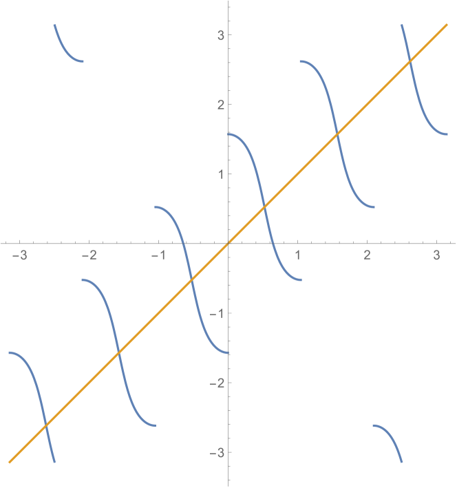
In order to define a map we need to consider the antipodal map , the corresponding group action, and the quotient . It is easy to see that is -equivariant, and it induces a map
This map now can be extended to a continuous map . For , it is the map represented in figure 1. The same happens for any : is an open subspace of the sphere of dimension (with components), which projects onto an open subspace of the projective space (with components).
(2.8) Remark.
Fixed point indices sum up to form the (local) Lefschetz number, and critical point Morse indices yield the Morse polynomial. Both give topological estimates on the number of central configurations, provided they are non-degenerate (and here Morse non-degenerate on the quotient, which is equivalent to say that the Jacobian of is non-degenerate at fixed points). The computations involve homology computations on configuration spaces or on projective configuration spaces. See [20], [21], [19], [13], and [14].
Now, for each choice of masses there is a (compact) subset of central configurations in . It can be proven that the set is non-empty (the minima of the potential yield central configurations). On the other hand, as already Moulton set forth, there is the inverse problem of central configurations: We consider, after Albouy–Moeckel [3], the inverse problem for central configurations: given a configuration of bodies, find positive masses which make it central. We consider only collinear configurations (), and we refer for details and further references on the inverse problem to [3], [18], [24], [5], [11].
3 The inverse collinear central configurations problem: simplex-valued maps
Now we reformulate the inverse collinear problem in a quotient space. First, re-define : now it does not depend on the masses. Consider the orthogonal projection of (with respect to the standard euclidean scalar product in , i.e. the projection parallel to the vector ). Then the inverse problem for a configuration has solutions (i.e. positive masses such that the configuration is central with respect with this choice of masses and its center of mass) if and only if there exists with positive coefficients such that .
The space has dimension : let denote the -dimensional subspace
Consider the open cone
It is homeomorphic to , where is the closure of in : it is a -simplex, and its faces are given by the equations
the simplex itself is given by the inequalities with and .
A simple computation gives the following lemma (cf. [11] for details and [9] for more on mutual differences).
(3.1) Lemma.
Let , for . Then are a linear system of coordinates on , and if and only if for . Moreover, the simplex is the standard simplex in , and are barycentric coordinates with respect to its vertices.
In -coordinates then for a configuration there is a solution to the inverse problem if and only if there exists , all positive, such that
| ((3.2)) |
Let denote the matrix with entries . Note that the sums of the entries in the -th column is
| ((3.3)) |
Let be a configuration. Let denote the -th column of the matrix . Then, by ((3.3)), belongs to the half-space of determined by the inequality .
As a consequence, for each the vector
belongs to (the sum of its components is ).
(3.4) Theorem.
Let be the multi-valued map defined as follows: for each the image is the convex hull (which is a finite union of simplices) of the points
for . Then the map is continuous and there is a solution to the inverse central configuration problem for the configuration if and only if .
(3.5) Remark.
A priori the dimension of the simplices in could be ; as a corollary of Theorems (2.13) and (2.17) of [11], at least for small, the columns of are always in general position (that is, the dimension of the simplices of is equal to ).
(3.6) Example ().
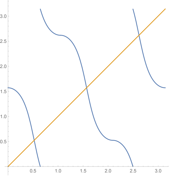
For , it is well-known that for the inverse problem has solutions for all configurations. It is in fact true for every , and it can be seen for in figure 2.
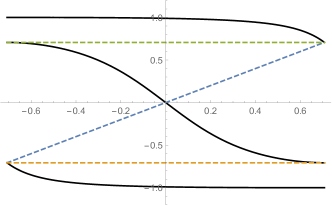
In order to visualize it, consider the homeomorphism , which sends the interval to the upper unit semicircle, and the interval to the arc of the unit circle with endpoints in . Rotate in clockwise and project it radially onto (this last step is not strictly necessary): then consider the corresponding three columns , and of the matrix , and their images in , and the projections on the unit circle (actually, the semicircle with ). Then rotating counter-clockwise by and taking the inverse of the homeomorphism gives the three maps
represented in figure 2, with . Now, it is clear that (where means the convex hull of the following list of points), and if (and hence ) , while if (and hence ) .
(3.7) Example ().
In this case the matrix ((3.2)) is
The -simplex and the plane can be projected on the unit sphere, as in figure 3.
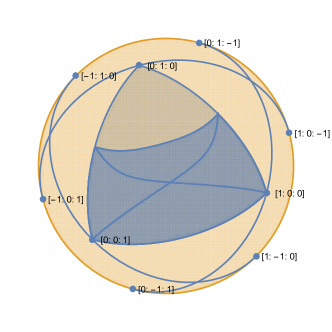
The simplex is represented together with the lines of equation in . Now it is not possible to visualize the maps , , and from to , defined as in the previous example. But after renormalization it is possible to consider the restrictions of to the three faces of , for , as follows. The matrix as will be (up to norms of the columns):
since for each . Recall that the matrix for the three particles is
hence the limiting as has a submatrix which corresponds to the columns of the problem with . The same computation can be performed for the other columns: it happens that the restrictions of to the faces of the simplex are nothing but the maps defined with , , and for suitable choice of masses. For further details on such self-map, see [11].
Acknowledgements
I would like to thank the organizers and the participants of the Nielsen Theory and Related Topics conference held in Kortrijk June 3–7, 2019. In particular, I would like to thank Jan Andres, Peter Wong and Daciberg Gonçalves for very interesting discussions on this topic, among others.
References
- [1] A. Albouy, Open Problem 1: Are Palmore’s “Ignored Estimates” on the Number of Planar Central Configurations Correct?, Qualitative Theory of Dynamical Systems, 14 (2015), pp. 403–406.
- [2] A. Albouy and V. Kaloshin, Finiteness of central configurations of five bodies in the plane, Annals of Mathematics, 176 (2012), pp. 535–588.
- [3] A. Albouy and R. Moeckel, The Inverse Problem for Collinear Central Configurations, Celestial Mechanics and Dynamical Astronomy, 77 (2000), pp. 77–91.
- [4] H. E. Buchanan, On certain determinants connected with a problem in celestial mechanics, Bulletin of the American Mathematical Society, 15 (1909), pp. 227–232.
- [5] C. Davis, S. Geyer, W. Johnson, and Z. Xie, Inverse problem of central configurations in the collinear 5-body problem, Journal of Mathematical Physics, 59 (2018), p. 052902.
- [6] E. R. Fadell and S. Y. Husseini, Geometry and Topology of Configuration Spaces, Springer Monographs in Mathematics, Springer Berlin Heidelberg, Berlin, Heidelberg, 2001.
- [7] D. L. Ferrario, Planar central configurations as fixed points, Journal of Fixed Point Theory and Applications, 2 (2007), pp. 277–291.
- [8] D. L. Ferrario, Fixed point indices of central configurations, Journal of Fixed Point Theory and Applications, 17 (2015), pp. 239–251.
- [9] , Central configurations and mutual differences, SIGMA. Symmetry, Integrability and Geometry. Methods and Applications, 13 (2017), pp. Paper No. 021, 11.
- [10] , Central configurations, Morse and fixed point indices, Bulletin of the Belgian Mathematical Society. Simon Stevin, 24 (2017), pp. 631–640.
- [11] , Pfaffians and the inverse problem for collinear central configurations, to appear in Celestial Mechanics and Dynamical Astronomy, (2020), p. 20.
- [12] M. Hampton and R. Moeckel, Finiteness of relative equilibria of the four-body problem, Inventiones mathematicae, 163 (2006), pp. 289–312.
- [13] C. K. McCord, Planar central configuration estimates in the n-body problem, Ergodic Theory and Dynamical Systems, 16 (1996), pp. 1059–1070.
- [14] J. C. Merkel, Morse Theory and Central Configurations in the Spatial N-body Problem, Journal of Dynamics and Differential Equations, 20 (2008), pp. 653–668.
- [15] R. Moeckel, On central configurations, Mathematische Zeitschrift, 205 (1990), pp. 499–517.
- [16] , Central configurations, in Central Configurations, Periodic Orbits, and Hamiltonian Systems, Adv. Courses Math. CRM Barcelona, Birkhäuser/Springer, Basel, 2015, pp. 105–167.
- [17] F. R. Moulton, The straight line solutions of the problem of $n$ bodies, Annals of Mathematics. Second Series, 12 (1910), pp. 1–17.
- [18] T. Ouyang and Z. Xie, Collinear Central Configuration in Four-Body Problem, Celestial Mechanics and Dynamical Astronomy, 93 (2005), pp. 147–166.
- [19] F. Pacella, Central configurations of the N-body problem via equivariant Morse theory, Archive for Rational Mechanics and Analysis, 97 (1987), pp. 59–74.
- [20] J. I. Palmore, Classifying relative equilibria. I, Bulletin of the American Mathematical Society, 79 (1973), pp. 904–908.
- [21] , Classifying relative equilibria. II, Bulletin of the American Mathematical Society, 81 (1975), pp. 489–491.
- [22] S. Smale, Topology and mechanics. II, Inventiones mathematicae, 11 (1970), pp. 45–64.
- [23] Z. Xia, Central configurations with many small masses, Journal of Differential Equations, 91 (1991), pp. 168–179.
- [24] Z. Xie, An analytical proof on certain determinants connected with the collinear central configurations in the $n$-body problem, Celestial Mechanics and Dynamical Astronomy, 118 (2014), pp. 89–97.
Address:
DL Ferrario
Department of Mathematics and Applications
University of Milano–Bicocca
Via R. Cozzi 55
20125 Milano – Italy
email: davide.ferrario@unimib.it