Abstract

This paper develops a technique allowing one to prove the convergence of a class of series of multiple integrals which corresponds to the form factor expansion of space-like separated two-point functions in the 1+1 dimensional massive integrable Sinh-Gordon quantum field theory.

MSC Classification : 82B23, 81Q80

1 Introduction

1.1 The physical background of the problem

The S-matrix program, initiated by Heisenberg [24] and Wheeler [49], was actively investigated in the 60s and 70s. Its conclusions where rather unsatisfactory in spacial dimensions higher than one: on the one hand due to the triviality of the S-matrix as soon as a given model exhibits a local conservation law other than the energy-momentum [15] and, on the other hand, due to the incapacity of constructing viable, explicit, S-matrices for any model missing such properties. However, the situation turned out to be drastically different for quantum field theories in 1+1 dimensions. The pioneering work of Gryanik and Vergeles [22] developed the first aspects of a method allowing one to determine S-matrices for quantum analogues of classical 1+1 dimensional field theories having an infinite set of independent local integrals of motion. It turns out that the existence of analogous conservation laws on the quantum level heavily constrains the classes of "in/out" asymptotic states that can be connected by the S-matrix. The reasoning of [22] applies to the case of models only exhibiting one type of asymptotic particles, the main example being given by the quantum Sinh-Gordon model. In those cases, the S-matrix is diagonal and thus fully described by one scalar function of the relative "in" rapidities of the two particles.

Dealing with the case of models having several types of asymptotic particles, some of equal masses and others realised as bound states of the former, turned out to be more involved. An archetype of such models is given by the Sine-Gordon quantum field theory. Building on the factorisability of the $n$-particle S-matrix into two-particle processes and on the independence of the order in which a three particle scattering process arises from a concatenation of two-particle processes -which is captured by the celebrated Yang-Baxter equation [8, 50]- Zamolodchikov derived the S-matrix of the Sine-Gordon model in the soliton-antisoliton sector [52] and managed to argue the model’s asymptotic particles content upon relying on Faddeev-Korepin’s [33] semi-classical quantisation results of the solitons in the classical Sine-Gordon model. Later, the S-matrix related to the soliton bound-state sectors, built out from the so-called breathers, was given in [27]. This provided the full S-matrix of the model since all asymptotic particles were now taken under consideration. Since then, S-matrices of many other models have been found, see e.g. [3, 51]. In fact, the factorisability of the $n$-particle S-matrix into two-particle processes was later established by Iagolnitzer within the S matrix axiomatics for theories having one [25] or several [26] asymptotic particles, under the hypotheses of macrocausality, causal factorisation, absence of particle production, conservation of individual particle momenta throughout the scattering and validity of the Yang-Baxter equation in the case of models having multiple asymptotic particles with internal degrees of freedom. Later, Parke [38] argued, on a more loose level of rigour, the same result solely in the presence of two extra conserved quantities in addition to the energy-momentum conservation.

Yet, the main physical interest does not reside in the per se calculation of S-matrices -which is just an intermediate tool in reaching the goal- but rather in being able to obtain a thorough description of correlation functions which are the observables being directly measured in experiments. Doing so may be achieved by obtaining the matrix elements of the local operators in the theory taken between the asymptotic states. Such quantities are called form factors. The full characterisation of the S matrix of the Sine-Gordon model allowed Weisz [48] to argue an expression for a specific form factor of the model: the matrix element of the electromagnetic current operator taken between an incoming and outgoing solition. The approach allowing one to calculate systematically the form factors in massive integrable 1+1 dimensional quantum field theories starting from the S-matrix has been initiated by Karowski, Weisz [28] who wrote down a set of equation satisfied by a model’s n-particle form factors and provided closed expressions for two particle form factors in several models. The calculation of form factors was subsequently addressed within the recently developed quantum inverse scattering method [19] which allowed to set up a quantum version of the Gelfand-Levitan-Marchenko equations allowing one to describe some of the operators arising in the quantum field theory model by means of solutions to certain singular integral equations involving free quantum fields satisfying the Faddeev-Zamolodchikov algebra. Their iterative solution expresses formally the quantum fields in terms of series of multiple integrals involving the free fields. The carry out of this program was implemented by Smirnov on the example of the Sine-Gordon model in the works [40, 41, 42]. This allowed him to obtain combinatorial expressions for the form factors of the exponential of the field operator, this for all types of asymptotic particles of the theory, in particular, reproducing the formulae for certain two-particle form factors derived earlier by Karowski, Weisz [28]. Smirnov’s approach was improved in the works [43, 44] where a set of auxiliary equations satisfied by the form factors was singled out and solved explicitly. This provided the first fully explicit representations for all the form factors of the Sine-Gordon model. Around that period Khamitov [29] constructed certain local operators for the quantisation of the classical 1+1 dimensional Sinh-Gordon field theory by means of formally solving the associated system of Gel’fand-Levitan-Marchenko equations for the exponentials of the field operators. He then showed, by using certain identities established by Kirillov [30], that the final combinatorial expressions he got for the form factors do ensure that the associated operators satisfy the CPT invariance and the local commutativity, viz. that two local operators located at the space-time points $\boldsymbol{x}$ and $\boldsymbol{y}$, with $\boldsymbol{x}-\boldsymbol{y}$ being a space-like vector, commute. I stress that this property is the necessary ingredient for having a causal theory. This approach opened up an important change of perspective in the construction of a quantum counterpart of a integrable classical field theory in that once one is able to propose some expressions, be it combinatoral or fully explicit, for the form factors of local operators taken between asymptotic states and then check independently that these satisfy CPT invariance and ensure that the operators satisfy local commutativity, then one may assert that one has built a per se quantum field theory in that the fundamental requirements thereof are satisfied.

This point of view was raised to its full glory by Kirillov, Smirnov [31, 32] on the example of the massive Thirring model. The authors postulated, as an axiomatic first input of the construction, a set of equations satisfied by the form factors of the model and which involve the model’s S-matrix: this setting constitutes what is called nowadays the bootstrap program for the form factors. Those bootstrap equations contain some of the equation already argued in [28], but also additional ones. It was shown by Kirillov, Smirnov [31, 32] that operators whose form factors satisfy the bootstrap equations do satisfy the local commutativity property. Hence, in the case of massive quantum integrable field theories, the bootstrap equations can be taken as an axiomatic input of the theory. The resolution of the bootstrap equations, if possible, then allows one to define the local operators of the theory as matrix operator. The resolution of the bootstrap program was systematised over the years and these efforts led to explicit expressions for the form factors of local operators in numerous 1+1 dimensional massive quantum field theories, see e.g. [47]. The first expressions for the form factors were rather combinatorial in nature. Later, a substantial progress was achieved in simplifying the latter, in particular by exhibiting a deeper structure at their root. Notably, one can mention the free field based approach, also called angular quantisation, to the calculation of form factors. It was introduced by Lukyanov [36] and allowed to obtain convenient representations for certain form factors solving the bootstrap program. In particular, the construction led to closed and manageable expressions [13] for the form factors of the exponential of the field operators in the Sinh-Gordon and the Bullough-Dodd models. While first results were obtained for the form factors of operators going to primary operators the approach was generalised so as to encompass the form factors of the descendant operators [20, 35]. Also, one should mention that the free field construction of the form factors was refined into the $p$-function method, developed for the Sine-Gordon model in [5, 6, 7]. In this last approach, the non-trivial part of the form factors is expressed in terms of the action of some explicit operator on a simple symmetric function $p$ of many variables satisfying simple constraints. The choice of different $p$ functions gives rise to different local operators of the model.

1.2 The open mathematical problems related to integrable quantum field theories

Despite its importance, the sole construction of the form factors, even if very explicit, cannot be considered as the end of the story. Indeed, one may think of bootstrap program issued explicit expressions for the form factors as a way to define the local operators of the theory as matrix operators. Still, from the perspective of physics, one would like to go further, on the one hand, by being able to establish that such operators do enjoy certain properties and, on the other hand, by being able to characterise the model’s multi-point vacuum-to-vacuum correlation functions built out of such operators. The most essential of such properties is that the form factors obtained as solutions to the bootstrap program do give rise to local matrix operators which enjoy the local commutativity. As already mentioned, this was established by Kirillov and Smirnov [31, 32]. More precisely, they considered the matrix elements of the commutator taken between asymptotic states and expressed explicitly the products of the two local operators building up the commutator by using their matrix elements, the form factors. This thus expressed the commutator as a series of multiple integrals corresponding to a summation over all types of asymptotic states in the theory; namely a summation over all the various types of asymptotic particles, their internal degrees of freedom, and an integration over all their possible rapidities. Thus, on top of using various algebraic properties issuing from the boostrap equations, the Kirillov and Smirnov [31, 32] approach for establishing local commutativity also demands to rely on the convergence of the form factor series which are handled in the proof. In fact, this convergence property is what is also needed to ensure that the product of two matrix operators constructed through the bootstrap program is well-defined. A similar issue with convergence also arises when computing the multi-point vacuum-to-vacuum correlation functions. Indeed, by taking explicitly the products of each operator building up the correlator and averaging them over the vacuum, as in the case of the commutator, these may be expressed in terms of series of multiple integrals called form factor expansion. Hence, the very possibility to describe vacuum to vacuum multi-point correlation functions through their form factor expansions also demands to have established the convergence of these series of multiple integrals. While constituting an important mathematical ingredient for the rigorous construction of the bootstrap program solvable 1+1 dimensional massive quantum field theories, the convergence of form factors based series of multiple integrals is basically a completely open problem.

Numerical investigations, see e.g. [18], of the magnitude of the higher particle number form factors contribution to a two-point function seems to indicate that form factor expansions should converge quickly, this even for moderate separations between the operators. However, this does not constitute by any means a proof thereof. In fact, the sole proof of convergence was achieved by Smirnov, in an unpublished note, relatively to the form factor expansion of a specific two-point function in the Lee-Yang model [14, 53]. By using the very specific form of the form factors of certain operators in that model Smirnov was able to bound explicitly the form factors in terms of explicitly summable positive functions. The given proof was however lacking a generality that would allow it to be extended to other models where the expressions for the form factors are more intricate.

1.3 The main result

The purpose of this work is to develop a technique allowing one to prove the convergence of the form factor expansion associated with of the vacuum-to-vacuum space-like separated two-point functions of a large -if not full- class of local operators in the simplest massive 1+1 dimensional integrable quantum field theory: the quantum Sinh-Gordon model.

Those series takes the form

$$\mathcal{U}(\mathfrak{r})=\sum\limits_{N\geq 0}\mathcal{U}_{N}(r)\qquad\mathrm{with}\qquad r>0\;,$$ (1.1)

where the $N^{\mathrm{th}}$-summand takes the form

$$\mathcal{U}_{N}(r)\;=\;\int\limits_{\mathbb{R}^{N}}{\mathchoice{\dfrac{\mathrm{d}^{N}\beta}{N!(2\pi)^{N}}}{\dfrac{\mathrm{d}^{N}\beta}{N!(2\pi)^{N}}}{\frac{\mathrm{d}^{N}\beta}{N!(2\pi)^{N}}}{\frac{\mathrm{d}^{N}\beta}{N!(2\pi)^{N}}}}\prod\limits_{a\not=b}^{N}\Big{\{}\mathrm{e}^{{\mathchoice{\dfrac{1}{2}}{\dfrac{1}{2}}{\frac{1}{2}}{\frac{1}{2}}}\mathfrak{w}(\beta_{ab})}\Big{\}}\cdot\prod\limits_{a=1}^{N}\Big{\{}\mathrm{e}^{-r\,\cosh(\beta_{a})}\Big{\}}\cdot\mathcal{K}_{N}^{(\mathcal{O}_{1})}(\boldsymbol{\beta}_{N})\cdot\mathcal{K}_{N}^{(\mathcal{O}_{2})}(\boldsymbol{\beta}_{N})\;.$$ (1.2)

The function $\mathcal{K}_{N}^{(\mathcal{O})}\big{(}\boldsymbol{\beta}_{N}\big{)}$ is given in terms of a combinatorial sum involving a parameter $\mathfrak{b}\in]0\,;1/2[$:

$$\mathcal{K}_{N}^{(\mathcal{O})}\big{(}\boldsymbol{\beta}_{N}\big{)}\,=\;\sum\limits_{\boldsymbol{\ell}_{N}\in\{0,1\}^{N}}\prod\limits_{a<b}^{N}\bigg{\{}1\,-\,\mathrm{i}{\mathchoice{\dfrac{(\ell_{a}-\ell_{b})\cdot\sin[2\pi\mathfrak{b}]}{\sinh(\beta_{a}-\beta_{b})}}{\dfrac{(\ell_{a}-\ell_{b})\cdot\sin[2\pi\mathfrak{b}]}{\sinh(\beta_{a}-\beta_{b})}}{\frac{(\ell_{a}-\ell_{b})\cdot\sin[2\pi\mathfrak{b}]}{\sinh(\beta_{a}-\beta_{b})}}{\frac{(\ell_{a}-\ell_{b})\cdot\sin[2\pi\mathfrak{b}]}{\sinh(\beta_{a}-\beta_{b})}}}\bigg{\}}\cdot p_{N}^{(\mathcal{O})}\big{(}\boldsymbol{\beta}_{N}\mid\boldsymbol{\ell}_{N}\big{)}\;,$$ (1.3)

where $\boldsymbol{\ell}_{N}=(\ell_{1},\dots,\ell_{N})$. The functions $p_{N}^{(\mathcal{O})}$ depend on the operator considered. Several examples of such functions can be found in Subsection 2.4.

In its turn, the two-body interaction potential $\mathfrak{w}$ is defined, for $\lambda\in\mathbb{R}^{*}$, by means of the below Riemann integral of a slowly decaying oscillating integrand:

$$\mathfrak{w}(\lambda)\;=\;-4\int\limits_{\mathbb{R}}\mathrm{d}x\,{\mathchoice{\dfrac{\sinh(x\mathfrak{b})\cdot\sinh(x\hat{\mathfrak{b}})\cdot\sinh(\tfrac{1}{2}x)\cdot\cosh(x)}{x\cdot\sinh^{2}(x)}}{\dfrac{\sinh(x\mathfrak{b})\cdot\sinh(x\hat{\mathfrak{b}})\cdot\sinh(\tfrac{1}{2}x)\cdot\cosh(x)}{x\cdot\sinh^{2}(x)}}{\frac{\sinh(x\mathfrak{b})\cdot\sinh(x\hat{\mathfrak{b}})\cdot\sinh(\tfrac{1}{2}x)\cdot\cosh(x)}{x\cdot\sinh^{2}(x)}}{\frac{\sinh(x\mathfrak{b})\cdot\sinh(x\hat{\mathfrak{b}})\cdot\sinh(\tfrac{1}{2}x)\cdot\cosh(x)}{x\cdot\sinh^{2}(x)}}}\mathrm{e}^{\mathrm{i}\frac{\lambda x}{\pi}}\;,\qquad\mathrm{with}\qquad\hat{\mathfrak{b}}={\mathchoice{\dfrac{1}{2}}{\dfrac{1}{2}}{\frac{1}{2}}{\frac{1}{2}}}-\mathfrak{b}\;.$$ (1.4)

Standard techniques of complex analysis entail that $\mathfrak{w}$ has a logarithmic singularity at the origin $\mathfrak{w}(\lambda)\;=\;2\ln|\lambda|+\mathrm{O}(1)$ and decays to zero exponentially fast at $\pm\infty$. I refer to Section 3 for more details on why form factor expansions of the vacuum-to-vacuum space-like separated two-point functions are represented by the series of multiple integrals given above. There one will also find the discussion of the well-definiteness of the multiple integrals $\mathcal{U}_{N}(r)$.

The main result of this paper is gathered in Theorem 1.1 below.

Theorem 1.1.

Let $p_{N}^{(\mathcal{O}_{1})},p_{N}^{(\mathcal{O}_{2})}$ be bounded as

$$\big{|}p_{N}^{(\mathcal{O}_{k})}\big{(}\boldsymbol{\beta}_{N}\mid\boldsymbol{\ell}_{N}\big{)}\big{|}\;\leq\;C_{1}^{N}\cdot\prod\limits_{a=1}^{N}\mathrm{e}^{C_{2}|\beta_{a}|^{s}}$$ (1.5)

for some $N$-independent constants $C_{1},C_{2},s>0$.

Then, for any $r_{0}>0$, the series defining the function $\mathcal{U}(r)$ converges uniformly in

$$r\in[r_{0}\,;+\infty[$$ (1.6)

and one has the upper bound

$$\big{|}\mathcal{U}_{N}(r)\big{|}\;\leq\;\exp\Bigg{[}-{\mathchoice{\dfrac{3\pi^{4}\mathfrak{b}\,\hat{\mathfrak{b}}\cdot N^{2}}{4\cdot(\ln N)^{3}}}{\dfrac{3\pi^{4}\mathfrak{b}\,\hat{\mathfrak{b}}\cdot N^{2}}{4\cdot(\ln N)^{3}}}{\frac{3\pi^{4}\mathfrak{b}\,\hat{\mathfrak{b}}\cdot N^{2}}{4\cdot(\ln N)^{3}}}{\frac{3\pi^{4}\mathfrak{b}\,\hat{\mathfrak{b}}\cdot N^{2}}{4\cdot(\ln N)^{3}}}}\cdot\bigg{\{}1+\mathrm{O}\Big{(}{\mathchoice{\dfrac{1}{\ln N}}{\dfrac{1}{\ln N}}{\frac{1}{\ln N}}{\frac{1}{\ln N}}}\Big{)}\bigg{\}}\Bigg{]}\;.$$ (1.7)

I stress that the remainder is not uniform in $r\rightarrow{0}^{+}$ in accordance with the expected power-law in $r$ ultraviolet $r\rightarrow 0^{+}$ behaviour of $\mathcal{U}(r)$. Indeed, then one expect the series to loose its convergence properties and $\mathcal{U}(r)$ should exhibit a power-law behaviour in $r\rightarrow 0^{+}$.

The technique allowing one to establish this result takes its root in the probabilistic approach to extracting the large-$N$ behaviour of multiple integrals arising in random matrix theory and its refinements to more complex multiple integrals [2, 4], builds on certain features of potential theory [39], singular integral equations of truncated Wiener-Hopf type [37] and the Deift-Zhou non-linear steepest descent [17] asymptotic analysis of matrix valued Riemann–Hilbert problems. To start with, one establishes an upper bound on $\big{|}\mathcal{U}_{N}(r)\big{|}$ in terms of certain auxiliary $N$-fold integrals only involving one and two-body interactions between the integration variables. After some reductions, the large-$N$ behaviour of the auxiliary integral is then estimated in terms of the infimum over the space of probability measures on $\mathbb{R}$ of the quadratic functional

$$\mathcal{E}_{N}^{(+)}\big{[}\sigma\big{]}\,=\,{\mathchoice{\dfrac{\varkappa}{N}}{\dfrac{\varkappa}{N}}{\frac{\varkappa}{N}}{\frac{\varkappa}{N}}}\int\limits\cosh(\ln Ns)\,\mathrm{d}\sigma(s)\,-\,{\mathchoice{\dfrac{1}{2}}{\dfrac{1}{2}}{\frac{1}{2}}{\frac{1}{2}}}\int\limits\mathfrak{w}^{(+)}\Big{(}\ln N(s-u)\Big{)}\cdot\mathrm{d}\sigma(s)\,\mathrm{d}\sigma(u)\;,\qquad\varkappa={\mathchoice{\dfrac{r}{2}}{\dfrac{r}{2}}{\frac{r}{2}}{\frac{r}{2}}}\;,$$ (1.8)

where

$$\mathfrak{w}^{(+)}(u)\;=\;\mathfrak{w}(u)+{\mathchoice{\dfrac{1}{2}}{\dfrac{1}{2}}{\frac{1}{2}}{\frac{1}{2}}}\ln\Bigg{(}{\mathchoice{\dfrac{\sinh(u+2\mathrm{i}\pi\mathfrak{b})\sinh(u-2\mathrm{i}\pi\mathfrak{b})}{\sinh^{2}(u)}}{\dfrac{\sinh(u+2\mathrm{i}\pi\mathfrak{b})\sinh(u-2\mathrm{i}\pi\mathfrak{b})}{\sinh^{2}(u)}}{\frac{\sinh(u+2\mathrm{i}\pi\mathfrak{b})\sinh(u-2\mathrm{i}\pi\mathfrak{b})}{\sinh^{2}(u)}}{\frac{\sinh(u+2\mathrm{i}\pi\mathfrak{b})\sinh(u-2\mathrm{i}\pi\mathfrak{b})}{\sinh^{2}(u)}}}\Bigg{)}$$ (1.9)

so that $\mathfrak{w}^{(+)}(u)=\ln|u|+\mathrm{O}(1)$ at the origin. This stage of the analysis ultimately yields the upper bound

$$\big{|}\mathcal{U}_{N}(r)\big{|}\;\leq\;\exp\Bigg{\{}-N^{2}\cdot\mathrm{inf}\Big{\{}\mathcal{E}_{N}^{(+)}\big{[}\sigma\big{]}\;:\;\sigma\in\mathcal{M}^{1}(\mathbb{R})\Big{\}}\,+\,\mathrm{O}\big{(}(\ln N)^{2}N\big{)}\Bigg{\}}\;.$$ (1.10)

Since $\mathcal{E}_{N}^{(+)}$ depends itself on $N$, the infimum does depend on $N$ so that to conclude relatively to the convergence of the series one needs to evaluate it explicitly, at least to the leading order in $N$, and then to check that the infimum has strictly positive large-$N$ behaviour which dominates $(\ln N)^{2}/N$ in the large-$N$ limit.

To start with, it is shown that $\mathcal{E}_{N}^{(+)}$ admits a unique minimiser $\sigma_{\mathrm{eq}}^{(N)}$ on $\mathcal{M}^{1}(\mathbb{R})$. $\sigma_{\mathrm{eq}}^{(N)}$ is shown to be Lebesgue continuous with a density supported on a single interval which satisfies a singular integral equation of truncated Wiener-Hopf type. Such integral operators were extensively studied by Krein’s school and the solution may be expressed in terms of the solution to a $2\times 2$ matrix Riemann–Hilbert problem, see [37]. The presence of a parameter blowing up with $N$ in this problem allows one to apply the Deift-Zhou non-linear steepest descent method so as to produce a solution to this matrix Riemann–Hilbert problem in the large-$N$ regime. In this way, one is able to express $\mathcal{E}_{N}^{(+)}\big{[}\sigma_{\mathrm{eq}}^{(N)}\big{]}$ in terms of the Riemann–Hilbert problem data and then build on the established large-$N$ behaviour of its solution so as to extract the leading large-$N$ behaviour of $\mathcal{E}_{N}^{(+)}\big{[}\sigma_{\mathrm{eq}}^{(N)}\big{]}$. This, finally, yields Theorem 1.1.

The upper bound on $\mathcal{U}_{N}(r)$ obtained in Theorem 1.1 may be put in parallel with the large-$N$ behaviour arising in the study of partition functions of $\beta$-ensembles or the closely connected random matrix models. These take the form

$$\mathscr{Z}_{N}\;=\;\int\limits_{\mathbb{R}^{N}}\mathrm{d}^{N}\lambda\prod\limits_{a<b}^{N}|\lambda_{a}-\lambda_{b}|^{\beta}\cdot\prod\limits_{a=1}^{N}\mathrm{e}^{-NV(\lambda_{a})}\;.$$ (1.11)

It is a classical result, see e.g. [2, 10], that for a large class of potentials $V$ leading to the so-called on-cut regime $\mathscr{Z}_{N}$ admits, for any $k\geq 0$, the large-$N$ asymptotic expansion

$$\mathscr{Z}_{N}\;=\;C_{N}\exp\Bigg{\{}-N^{2}F_{0}\,+\,\sum\limits_{p=1}^{k+1}N^{2-p}F_{p}\;+\;\mathrm{O}\big{(}N^{-k}\big{)}\Bigg{\}}$$ (1.12)

The first term of the asymptotics is called the free energy and $C_{N}$ is an explicit, potential $V$ independent sequence related to a Selberg integral. In the upper bound (1.7) given in Theorem 1.1, there appears an additional $\ln N$ scale in the large-$N$ asymptotics. Thus, comparing with the above result for $\beta$-ensembles, all looks like one ends up with a free energy that is $N$-dependent, viz. $F_{0}\hookrightarrow F_{0}(N)$ such that $F_{0}(N)\mathrel{\underset{N\rightarrow+\infty}{{[}1]{$\sim$}}}f_{0}/(\ln N)^{3}$. One could be tempted to argue that all of such a large-$N$ behaviour is due to (1.7) being an upped bound so that, if one were to access to the true asymptotic behaviour of $\mathcal{U}_{N}(r)$, then the latter would rather follow the typical random matrix like structure (1.12). I would like to stress that it would notation be so since the two scales -$N$ and $\ln N$- are natural to this problem. While the leading asymptotic behaviour of $\mathcal{U}_{N}(r)$ might surely differ from the upper bound (1.7), one still expects that

$$\ln\big{[}\mathcal{U}_{N}(r)\big{]}\;\simeq\;-N^{2}(\ln N)^{p}\Bigg{\{}Q_{0,0}\;+\;\sum\limits_{\begin{subarray}{c}(s,\ell)\\ \not=(0,0)\end{subarray}}{\mathchoice{\dfrac{Q_{s,\ell}}{N^{\ell}(\ln N)^{s}}}{\dfrac{Q_{s,\ell}}{N^{\ell}(\ln N)^{s}}}{\frac{Q_{s,\ell}}{N^{\ell}(\ln N)^{s}}}{\frac{Q_{s,\ell}}{N^{\ell}(\ln N)^{s}}}}\Bigg{\}}$$ (1.13)

in the sense of a two-scaled asymptotic expansion. The presence of the two-scales -$N$ and $\ln N$- stems from the lack of a prefactor of $N$ in the exponentially growing at infinity one-body confining potential: $r\,\cosh(\beta)$, which has to compete with $N^{2}$ terms issuing from the two-body interaction $\mathfrak{w}(\beta-\beta^{\prime})$ which is repulsive on short distances. Only after going to a $\ln N$ dilatation scale in between the integration variables do the one and two body interactions become of the same scale in $N$ for typical, bounded, values of the new integration variables. The source of the $1/\big{(}\ln N\big{)}^{3}$ prefactor in the upper bound is rather subtle and I do not have a nice, heuristical interpretation thereof.

To conclude the presentation of the main results of this work, I will comment on the generality of the method. While developed for the case of a specific two-point function in the Sinh-Gordon model with operators being separated by space-time intervals, it is clear that the method is applicable to a wide range of situations. First of all, upon a few additional technical steps, the method will allow to also determine convergence in the case of time-like separation between the operators building up a two point function. Moreover, there does not seem to appear any obstruction so as to apply the method so as to prove the convergence of multi-point correlation functions in the model as well as the one of other that the vacuum-to-vacuum expectation values. As such, upon appropriate modifications, this allows to finish the proof, for this model, of the causality property of the local operators constructed through the bootstrap program. Finally, the technique for proving the convergence of form factor expansions developed in this work only relies on very general properties of the form factors and not their detailed form. Hence, the method looks like a promising path which would allow one to solve the convergence problem of form factor expansions in more complex integrable quantum field theories such as the Sine-Gordon model.

Outline of the work

The paper is organised as follows. Section 2 reviews the bootstrap program issued results providing explicit expressions for the form factors of local operators in the 1+1 dimensional Sinh-Gordon model. Section 3 presents the general structure of the form factor expansion of two-point functions, in Euclidian space-time, of the model. I establish an upper bound for the $N^{\mathrm{th}}$ summand of this series in the case of space-like separated operators. It is shown in Section 4 that the large-$N$ behaviour of this upper bound can be estimated by solving a minimisation problem. The unique solvability of this minimisation problem is then established in Section 5. The characterisation of the minimiser is then reduced to the resolution of a singular integral equation of truncated Wiener-Hopf type in Section 6. Section 7 develops the non-linear steepest descent solution of an auxiliary matrix Riemann–Hilbert problem whose solution plays a central role in the inversion of the singular integral operator arising in the characterisation of the minimiser. Section 8 builds on these results so as to produce a closed form, for $N$ large enough, of this operator’s inverse. Then, Section 9 utilises these results so as to provide an explicit description of the equilibrium measure associated with the minimisation problem. Finally, Section 10 carries out the large-$N$ estimates of the minimisation problem what allows one to conclude relatively to the convergence of the series.

2 Form factors in the quantum Sinh-Gordon model

The classical Sinh-Gordon model describes the evolution of a scalar field $\varphi(x,t)$ under the partial differential equation

$$\Big{(}\partial_{t}^{2}-\partial_{x}^{2}\Big{)}\varphi\,+\,{\mathchoice{\dfrac{m^{2}}{g}}{\dfrac{m^{2}}{g}}{\frac{m^{2}}{g}}{\frac{m^{2}}{g}}}\sinh(g\varphi)\,=\,0$$ (2.1)

which is associated with the extremalisation condition for the action $\mathcal{S}[\varphi]=\int\limits\mathcal{L}(\varphi,\partial_{\mu}\varphi)\cdot\mathrm{d}^{2}x$ subordinate to the Lagrangian

$$\mathcal{L}(\varphi,\partial_{\mu}\varphi)\,=\,{\mathchoice{\dfrac{1}{2}}{\dfrac{1}{2}}{\frac{1}{2}}{\frac{1}{2}}}\partial_{\mu}\varphi\partial^{\mu}\varphi\,-\,{\mathchoice{\dfrac{m^{2}}{g^{2}}}{\dfrac{m^{2}}{g^{2}}}{\frac{m^{2}}{g^{2}}}{\frac{m^{2}}{g^{2}}}}\cosh(g\varphi)\;.$$ (2.2)

In infinite volume, the quantum field theory underlying to this classical field theory is associated with the Hilbert space

$$\mathfrak{h}_{\mathrm{SG}}\,=\,\bigoplus\limits_{n=0}^{+\infty}L^{2}(\mathbb{R}^{n}_{>})\qquad\mathrm{with}\qquad\mathbb{R}^{n}_{>}\;=\;\Big{\{}\boldsymbol{\beta}_{n}=(\beta_{1},\dots,\beta_{n})\in\mathbb{R}^{n}\;:\;\beta_{1}>\dots>\beta_{n}\Big{\}}\;.$$ (2.3)

Here $f\in L^{2}(\mathbb{R}^{n}_{>})$ has the physical interpretation of an "in", viz. incoming, asymptotic $n$-particle wave-packet. More precisely, on physical grounds, one interprets elements of the Hilbert space $\mathfrak{h}_{\mathrm{SG}}$ as parameterised by $n$-particles states, $n\in\mathbb{N}$, arriving, in the remote past, with well-ordered rapidities $\beta_{1}>\dots>\beta_{n}$. Such states are called asymptotic "in" states. Then, within this physical picture, as time goes by, the "in" particles approach each other, interact, scatter and finally travel again as free particles out of the system. Within such a scheme, an "out" $n$-particle state is then paramaterised by $n$ well-ordered rapidities $\beta_{1}<\dots<\beta_{n}$. In fact, one could equivalently associate the model with the Hilbert space

$$\bigoplus\limits_{n=0}^{+\infty}L^{2}(\mathbb{R}^{n}_{<})\qquad\mathrm{with}\qquad\mathbb{R}^{n}_{<}\;=\;\Big{\{}\boldsymbol{\beta}_{n}=(\beta_{1},\dots,\beta_{n})\in\mathbb{R}^{n}\;:\;\beta_{1}<\dots<\beta_{n}\Big{\}}\;,$$ (2.4)

in which elements of the $L^{2}(\mathbb{R}^{n}_{<})$ spaces have the physical interpretation of an "out", viz. outgoing in the distant future, asymptotic $n$-particle wave-packet.

Within the formalism of quantum field theory, the "in" and "out" states are connected by the model’s S matrix. In the case of the Sinh-Gordon 1+1 dimensional quantum field theory, the S-matrix was first determined in [22]. It corresponds to a diagonal scattering between the particles and takes the form

$$\boldsymbol{\texttt{S}}(\beta)\,=\,{\mathchoice{\dfrac{\tanh\big{[}\tfrac{1}{2}\beta-\mathrm{i}\pi\mathfrak{b}\big{]}}{\tanh\big{[}\tfrac{1}{2}\beta+\mathrm{i}\pi\mathfrak{b}\big{]}}}{\dfrac{\tanh\big{[}\tfrac{1}{2}\beta-\mathrm{i}\pi\mathfrak{b}\big{]}}{\tanh\big{[}\tfrac{1}{2}\beta+\mathrm{i}\pi\mathfrak{b}\big{]}}}{\frac{\tanh\big{[}\tfrac{1}{2}\beta-\mathrm{i}\pi\mathfrak{b}\big{]}}{\tanh\big{[}\tfrac{1}{2}\beta+\mathrm{i}\pi\mathfrak{b}\big{]}}}{\frac{\tanh\big{[}\tfrac{1}{2}\beta-\mathrm{i}\pi\mathfrak{b}\big{]}}{\tanh\big{[}\tfrac{1}{2}\beta+\mathrm{i}\pi\mathfrak{b}\big{]}}}}\qquad\mathrm{with}\qquad\mathfrak{b}\,=\,{\mathchoice{\dfrac{1}{2}}{\dfrac{1}{2}}{\frac{1}{2}}{\frac{1}{2}}}{\mathchoice{\dfrac{g^{2}}{8\pi+g^{2}}}{\dfrac{g^{2}}{8\pi+g^{2}}}{\frac{g^{2}}{8\pi+g^{2}}}{\frac{g^{2}}{8\pi+g^{2}}}}\;.$$ (2.5)

This S-matrix satisfies the unitarity $\boldsymbol{\texttt{S}}(\beta)\boldsymbol{\texttt{S}}(-\beta)=1$, and crossing $\boldsymbol{\texttt{S}}(\beta)=\boldsymbol{\texttt{S}}(\mathrm{i}\pi-\beta)$ symmetries. Moreover, the S matrix is $2\mathrm{i}\pi$ periodic in $\beta$ and has simple poles at

$$\beta\,\in\;\mathrm{i}\pi\,+\,2\mathrm{i}\pi\mathfrak{b}\,+\,2\mathrm{i}~\pi\mathbb{Z}\quad\mathrm{and}\quad\beta\,\in\;-2\mathrm{i}\pi\mathfrak{b}\,+\,2\mathrm{i}~\pi\mathbb{Z}\;.$$ (2.6)

For $g\in\mathbb{R}^{*}$, one has $0<\mathfrak{b}<1/2$, what ensures that S has no poles in the physical strip $0<\Im(\beta)<\pi$. This property is consistent with the absence of bound states in the model. The S-matrix has simple zeroes at

$$\beta\,\in\;\mathrm{i}\pi\,-\,2\mathrm{i}\pi\mathfrak{b}\,+\,2\mathrm{i}~\pi\mathbb{Z}\quad\mathrm{and}\quad\beta\,\in\;2\mathrm{i}\pi\mathfrak{b}\,+\,2\mathrm{i}~\pi\mathbb{Z}\;.$$ (2.7)

The two zeroes $\mathrm{i}\pi\,-\,2\mathrm{i}\pi\mathfrak{b}$ and $2\mathrm{i}\pi\mathfrak{b}$ belong to the physical strip and are related by the crossing symmetry

$$\mathfrak{b}\;\hookrightarrow\;\hat{\mathfrak{b}}\,=\,1/2-\mathfrak{b}\;.$$ (2.8)

This is obviously also a symmetry of the model’s S-matrix $\boldsymbol{\texttt{S}}(\beta)=\boldsymbol{\texttt{S}}(\beta)_{\mid\mathfrak{b}\hookrightarrow\hat{\mathfrak{b}}}$. This symmetry reflects the weak/strong duality of the theory, viz. the invariance of the model’s observables under the map $g\hookrightarrow 8\pi/g$.

In order to realise the quantum field theory of interest on $\mathfrak{h}_{\mathrm{SG}}$ one should provide a thorough and explicit description of the operator content of the model. In fact, one is interested mainly in so-called local operators which are thought of as objects located at the space-time point $\boldsymbol{x}=(x_{0},x_{1})$. Generically these will be denoted as $\mathcal{O}(\boldsymbol{x})$. The quantum Sinh-Gordon field theory is transitionally invariant, what means that the model is naturally endowed with a unitary operator $\boldsymbol{\texttt{U}}_{\boldsymbol{\texttt{T}}_{\boldsymbol{y}}}$ such that

$$\boldsymbol{\texttt{U}}_{\boldsymbol{\texttt{T}}_{\boldsymbol{y}}}\cdot\mathcal{O}(\boldsymbol{x})\cdot\boldsymbol{\texttt{U}}_{\boldsymbol{\texttt{T}}_{\boldsymbol{y}}}^{-1}\,=\,\mathcal{O}(\boldsymbol{x}+\boldsymbol{y})\;.$$ (2.9)

The translation operator acts diagonally in the asymptotic states’ Hilbert space $\mathfrak{h}_{\mathrm{SG}}$, namely for
$\boldsymbol{f}=(f^{(0)},\dots,f^{(n)},\dots)\in\mathfrak{h}_{\mathrm{SG}}$, it holds

$$\boldsymbol{\texttt{U}}_{\boldsymbol{\texttt{T}}_{\boldsymbol{y}}}\cdot\boldsymbol{f}\;=\;\Big{(}\boldsymbol{\texttt{U}}_{\boldsymbol{\texttt{T}}_{\boldsymbol{y}}}^{(0)}\cdot f^{(0)},\dots,\boldsymbol{\texttt{U}}_{\boldsymbol{\texttt{T}}_{\boldsymbol{y}}}^{(n)}\cdot f^{(n)},\dots\Big{)}\quad\mathrm{where}\quad\boldsymbol{\texttt{U}}_{\boldsymbol{\texttt{T}}_{\boldsymbol{y}}}^{(n)}\cdot f^{(n)}(\boldsymbol{\beta}_{n})\;=\;\exp\bigg{\{}\mathrm{i}\sum\limits_{a=1}^{n}\boldsymbol{p}(\beta_{a})\cdot\boldsymbol{y}\bigg{\}}f^{(n)}(\boldsymbol{\beta}_{n})$$ (2.10)

in which $\boldsymbol{p}(\beta)=\big{(}m\cosh(\beta),m\sinh(\beta)\big{)}$ and $\boldsymbol{x}\cdot\boldsymbol{y}$ stands for the Minkowski $2$-form $\boldsymbol{x}\cdot\boldsymbol{y}\,=\,x_{0}y_{0}-x_{1}y_{1}$.

In order to describe the action of a local operator $\mathcal{O}(\boldsymbol{x})$ on $\boldsymbol{f}=(f^{(0)},f^{(1)},\dots,)$ belonging to an appropriate dense subspace of $\mathfrak{h}_{\mathrm{SG}}$, within the bootstrap program, one first introduces the elementary building blocks of the action which arise as

$$\Big{(}\mathcal{O}(\boldsymbol{x})\cdot\boldsymbol{f}\Big{)}^{(0)}\;=\;\sum\limits_{m\geq 0}\;\int\limits_{\beta_{1}>\dots>\beta_{m}}\mathrm{d}^{m}\beta\;\mathcal{F}_{m;+}^{(\mathcal{O})}(\boldsymbol{\beta}_{m})\prod\limits_{a=1}^{m}\Big{\{}\mathrm{e}^{-\mathrm{i}\boldsymbol{p}(\beta_{a})\cdot\boldsymbol{x}}\Big{\}}f^{(m)}\big{(}\boldsymbol{\beta}_{m}\big{)}\;.$$ (2.11)

The oscillatory prefactor is simply a consequence of the translation invariance (2.9). The quantities $\mathcal{F}_{n}^{(\mathcal{O})}(\boldsymbol{\beta}_{n})$ are called form factors and are certain meromorphic functions in each of the variables $\beta_{a}$ belonging to the so-called physical strip $0\leq\Im(\beta_{a})\leq\pi$. $\mathcal{F}_{m;+}^{(\mathcal{O})}$ then corresponds to the $+$ boundary value on $\mathbb{R}^{m}$ of $\mathcal{F}_{m}^{(\mathcal{O})}(\boldsymbol{\beta}_{m})$, understood as

$$\mathcal{F}_{m;+}^{(\mathcal{O})}(\boldsymbol{\beta}_{m})\;=\;\lim_{\begin{subarray}{c}\boldsymbol{\epsilon}_{m}\rightarrow\,\boldsymbol{0}\\ \epsilon_{1}>\cdots>\epsilon_{m}>0\end{subarray}}\mathcal{F}_{m}^{(\mathcal{O})}(\boldsymbol{\beta}_{m}+\mathrm{i}\boldsymbol{\epsilon}_{m})\;.$$ (2.12)

These quantities, and the axiomatics leading to their characterisation within the bootstrap program, will be discussed below.

Within the bootstrap approach to quantum integrable field theories, the remaining part of the action of the operator may then be constructed out of the form factors. This procedure is, in fact, part of the axioms of the theory. More precisely, the component on higher particle number spaces of the operator’s action may be recast, for sufficiently regular functions $\boldsymbol{f}$, as

$$\Big{(}\mathcal{O}(\boldsymbol{x})\cdot\boldsymbol{f}\Big{)}^{(n)}(\boldsymbol{\gamma}_{n})\;=\;\sum\limits_{m\geq 0}\;\boldsymbol{\texttt{M}}_{\mathcal{O}}^{(m)}\Big{(}\boldsymbol{x}\,\mid\boldsymbol{\gamma}_{n}\Big{)}\big{[}f^{(m)}\big{]}\;,$$ (2.13)

in which $\boldsymbol{\texttt{M}}_{\mathcal{O}}^{(m)}\big{(}\boldsymbol{x}\,\mid\boldsymbol{\gamma}_{n}\big{)}$ are certain functions taking values in distributions which act on appropriate spaces of functions in $m$ variables. Note that their $x$ dependence follows readily from the translation invariance (2.9). It is convenient, in order to avoid heavy notations, to represent their action as

$$\boldsymbol{\texttt{M}}_{\mathcal{O}}^{(m)}\Big{(}\boldsymbol{x}\,\mid\boldsymbol{\gamma}_{n}\Big{)}\big{[}f^{(m)}\big{]}\;=\;\prod\limits_{a=1}^{n}\mathrm{e}^{\mathrm{i}\boldsymbol{p}(\gamma_{a})}\,\cdot\int\limits_{\beta_{1}>\dots>\beta_{m}}\mathrm{d}^{m}\beta\;\mathcal{M}_{\mathcal{O}}\Big{(}\boldsymbol{\gamma}_{n};\boldsymbol{\beta}_{m}\Big{)}\cdot\prod\limits_{a=1}^{m}\mathrm{e}^{-\mathrm{i}\boldsymbol{p}(\beta_{a})\cdot\boldsymbol{x}}\cdot f^{(m)}\big{(}\boldsymbol{\beta}_{m}\big{)}\;,$$ (2.14)

and where the integrals should be understood in a distributional sense, i.e. the quantities $\mathcal{M}_{\mathcal{O}}\big{(}\boldsymbol{x}\mid\boldsymbol{\gamma}_{n};\boldsymbol{\beta}_{m}\big{)}$ should be thought of as generalised functions. These generalised functions are postulated to satisfy an inductive reduction structure which, again, should be understood in the sense of distributions

$$\mathcal{M}_{\mathcal{O}}\Big{(}\boldsymbol{\alpha}_{n};\boldsymbol{\beta}_{m}\Big{)}\;=\;\mathcal{M}_{\mathcal{O}}\Big{(}(\alpha_{2},\dots,\alpha_{n});(\alpha_{1}+\mathrm{i}\pi,\boldsymbol{\beta}_{m})\Big{)}\\ \;+\;2\pi\sum\limits_{a=1}^{m}\delta_{\alpha_{1};\beta_{a}}\prod\limits_{k=1}^{a-1}\boldsymbol{\texttt{S}}(\beta_{k}-\alpha_{1})\cdot\mathcal{M}_{\mathcal{O}}\Big{(}(\alpha_{2},\dots,\alpha_{n});(\beta_{1},\dots,\widehat{\beta}_{a},\dots,\beta_{m})\Big{)}\;.$$ (2.15)

In the above expression, $\widehat{\beta}_{a}$ means that the variable $\beta_{a}$ should be omitted and $\delta_{x;y}$ refers to the Dirac mass distribution centred at $x$ and acting on functions of $y$. Note in particular that there is no problem with multiplication of distributions in the above formula since the variables are separated. Finally, the evaluation at $\alpha_{1}+\mathrm{i}\pi$ should be understood in the sense of a meromorphic continuation in the strip $0\leq\Im(z)\leq\pi$ from $\mathbb{R}$ up to $\mathbb{R}+\mathrm{i}\pi$. The recursion (2.15) is to be complemented with the initialisation condition $\mathcal{M}_{\mathcal{O}}\big{(}\boldsymbol{0}\mid\emptyset;\boldsymbol{\beta}_{n}\big{)}\;=\;\mathcal{F}_{n}^{(\mathcal{O})}(\boldsymbol{\beta}_{n})$. The recursion may be solved in closed form, see e.g. [31], although I will not discuss the form of this solution here in that it will play no role in the problem to be considered. However, it is clear from the structure of the recursion that the generalised functions $\mathcal{M}_{\mathcal{O}}\big{(}\boldsymbol{x}\mid\boldsymbol{\alpha}_{n};\boldsymbol{\beta}_{m}\big{)}$ can be expressed as linear combinations of terms involving the form factors dressed up by certain products of S-matrices and Dirac masses. This thus justifies the statement that the form factors are the elementary building blocks allowing one to define the action of the operators of the theory.

Finally, one should mention that the generalised functions $\mathcal{M}_{\mathcal{O}}\big{(}\boldsymbol{x}\mid\boldsymbol{\alpha}_{n};\boldsymbol{\beta}_{m}\big{)}$ are invariant under an overall shift of the rapidities what is a manifestation of the Lorentz invariance of the theory, namely that

$$\mathcal{M}_{\mathcal{O}}\Big{(}\boldsymbol{\alpha}_{n}+\theta\,\overline{\boldsymbol{e}}_{n};\boldsymbol{\beta}_{m}+\theta\,\overline{\boldsymbol{e}}_{m}\Big{)}\;=\;\mathrm{e}^{\theta\boldsymbol{\texttt{s}}_{\mathcal{O}}}\cdot\mathcal{M}_{\mathcal{O}}\Big{(}\boldsymbol{\alpha}_{n};\boldsymbol{\beta}_{m}\Big{)}$$ (2.16)

where $\boldsymbol{\texttt{s}}_{\mathcal{O}}$ is called the spin of the operator $\mathcal{O}$ while $\overline{\boldsymbol{e}}_{k}=(1,\dots,1)\in\mathbb{R}^{k}$.

One may readily connect this description with the formal picture usually encountered in quantum field theory. In that picture, the $\mathrm{in}/\mathrm{out}$ states of the particles with rapidities $\boldsymbol{\beta}_{n}$ are formally denoted as $\boldsymbol{\mathcal{A}}_{\mathrm{in}/\mathrm{out}}(\boldsymbol{\beta}_{n})$. Then, $\mathcal{M}_{\mathcal{O}}\Big{(}\boldsymbol{x}\,\mid\boldsymbol{\alpha}_{n};\boldsymbol{\beta}_{m}\Big{)}$ correspond to the matrix elements of the operator $\mathcal{O}(\boldsymbol{x})$ taken between two asymptotic states

$$\mathcal{M}_{\mathcal{O}}\Big{(}\boldsymbol{\alpha}_{n};\boldsymbol{\beta}_{m}\Big{)}\;=\;\Big{(}\boldsymbol{\mathcal{A}}_{\mathrm{in}}(\boldsymbol{\alpha}_{n}),\mathcal{O}(\boldsymbol{x})\boldsymbol{\mathcal{A}}_{\mathrm{in}}(\boldsymbol{\beta}_{m})\Big{)}\;,\quad\mathrm{where}\quad\boldsymbol{\beta}_{k}\,=\,\big{(}\beta_{1},\dots,\beta_{k}\big{)}\;.$$ (2.17)

In particular, one has that the form factors correspond to the vacuum-to-excited state matrix elements of the operator $\mathcal{O}(\boldsymbol{0})$:

$$\mathcal{F}_{n}^{(\mathcal{O})}(\boldsymbol{\beta}_{n})\;=\;\Big{(}\boldsymbol{\mathcal{A}}_{\mathrm{in}}(\emptyset),\mathcal{O}(\boldsymbol{0})\boldsymbol{\mathcal{A}}_{\mathrm{in}}(\beta_{1},\dots,\beta_{n})\Big{)}\;.$$ (2.18)

The recursive relation (2.15) may then be interpreted as issuing from the formal LSZ reduction formula [23]. See [5, 47] for more details.

2.1 The form factor axioms

The form factors are postulated to satisfy the below set of bootstrap equations [31]:

• $\mathcal{F}_{n}^{(\mathcal{O})}(\beta_{1},\dots,\beta_{a},\beta_{a+1},\dots,\beta_{n})\;=\;\boldsymbol{\texttt{S}}(\beta_{a}-\beta_{a+1})\cdot\mathcal{F}_{n}^{(\mathcal{O})}(\beta_{1},\dots,\beta_{a+1},\beta_{a},\dots,\beta_{n})$;

• $\mathcal{F}_{n}^{(\mathcal{O})}(\beta_{1}+2\mathrm{i}\pi,\beta_{2},\dots,\beta_{n})\;=\;\mathcal{F}_{n}^{(\mathcal{O})}(\beta_{2},\dots,\beta_{n},\beta_{1})\,=\,\prod\limits_{a=2}^{n}\Big{\{}\boldsymbol{\texttt{S}}(\beta_{a}-\beta_{1})\Big{\}}\cdot\mathcal{F}_{n}^{(\mathcal{O})}(\beta_{1},\dots,\beta_{n})$;

• $\mathcal{F}_{n}^{(\mathcal{O})}$ is meromorphic in each variable taken singly throughout the strip $0\leq\Im(\beta)\leq 2\pi$. Its only poles are simple and located at $\mathrm{i}\pi$ shifted rapidities. The residues at these poles enjoy the inductive structure

  $$-\mathrm{i}\,\mathrm{Res}\bigg{(}\mathcal{F}_{n+2}^{(\mathcal{O})}(\alpha+\mathrm{i}\pi,\beta,\beta_{1},\dots,\beta_{n})\cdot\mathrm{d}\alpha\,,\,\alpha=\beta\bigg{)}\;=\;\bigg{\{}1\,-\,\prod\limits_{a=1}^{n}\boldsymbol{\texttt{S}}(\beta-\beta_{a})\bigg{\}}\cdot\mathcal{F}_{n}^{(\mathcal{O})}(\beta_{1},\dots,\beta_{n})\;;$$ (2.19)

• $\mathcal{F}_{n}^{(\mathcal{O})}$ are boost invariant

  $$\mathcal{F}_{n}^{(\mathcal{O})}(\beta_{1}+\Lambda,\dots,\beta_{n}+\Lambda)\;=\;\mathrm{e}^{\Lambda\boldsymbol{\texttt{s}}_{\mathcal{O}}}\cdot\mathcal{F}_{n}^{(\mathcal{O})}(\beta_{1},\dots,\beta_{n})\;.$$ (2.20)

In fact, the above equations can be taken as a set of axioms satisfied by the form factors of the theory.

2.2 The $2$-particle sector solution

The form factor axioms in the two-particle sector $n=2$ take the particularly simple form of a scalar Riemann–Hilbert problem in one variable for a holomorphic function F in the strip $0\leq\Im(\beta)\leq 2\pi$ that has no zeroes in this strip, behaves as $\boldsymbol{\texttt{F}}(\beta)=1\,+\,\mathrm{O}\big{(}\beta^{-2}\big{)}$ as $\Re(\beta)\rightarrow\pm\infty$ uniformly in $0\leq\Im(\beta)\leq 2\pi$ and satisfies

$$\boldsymbol{\texttt{F}}(\beta)\,=\,\boldsymbol{\texttt{F}}(-\beta)\cdot\boldsymbol{\texttt{S}}(\beta)\qquad\mathrm{and}\qquad\boldsymbol{\texttt{F}}(\mathrm{i}\pi-\beta)\,=\,\boldsymbol{\texttt{F}}(\mathrm{i}\pi+\beta)\;.$$ (2.21)

One can effectively solve these equations by observing that S admits the integral representation

$$\boldsymbol{\texttt{S}}(\beta)\;=\;\exp\Bigg{\{}8\int\limits_{0}^{+\infty}\mathrm{d}x{\mathchoice{\dfrac{\sinh(x\mathfrak{b})\cdot\sinh(x\hat{\mathfrak{b}})\cdot\sinh(\tfrac{1}{2}x)}{x\sinh(x)}}{\dfrac{\sinh(x\mathfrak{b})\cdot\sinh(x\hat{\mathfrak{b}})\cdot\sinh(\tfrac{1}{2}x)}{x\sinh(x)}}{\frac{\sinh(x\mathfrak{b})\cdot\sinh(x\hat{\mathfrak{b}})\cdot\sinh(\tfrac{1}{2}x)}{x\sinh(x)}}{\frac{\sinh(x\mathfrak{b})\cdot\sinh(x\hat{\mathfrak{b}})\cdot\sinh(\tfrac{1}{2}x)}{x\sinh(x)}}}\sinh\Big{(}\tfrac{x\beta}{\mathrm{i}\pi}\Big{)}\Bigg{\}}\quad\mathrm{with}\quad\hat{\mathfrak{b}}\,=\,{\mathchoice{\dfrac{1}{2}}{\dfrac{1}{2}}{\frac{1}{2}}{\frac{1}{2}}}\,-\,\mathfrak{b}\;.$$ (2.22)

Following e.g. the method of [28], this yields that

$$\boldsymbol{\texttt{F}}(\beta)\;=\;\exp\Bigg{\{}-4\int\limits_{0}^{+\infty}\mathrm{d}x{\mathchoice{\dfrac{\sinh(x\mathfrak{b})\cdot\sinh(x\hat{\mathfrak{b}})\cdot\sinh(\tfrac{1}{2}x)}{x\sinh^{2}(x)}}{\dfrac{\sinh(x\mathfrak{b})\cdot\sinh(x\hat{\mathfrak{b}})\cdot\sinh(\tfrac{1}{2}x)}{x\sinh^{2}(x)}}{\frac{\sinh(x\mathfrak{b})\cdot\sinh(x\hat{\mathfrak{b}})\cdot\sinh(\tfrac{1}{2}x)}{x\sinh^{2}(x)}}{\frac{\sinh(x\mathfrak{b})\cdot\sinh(x\hat{\mathfrak{b}})\cdot\sinh(\tfrac{1}{2}x)}{x\sinh^{2}(x)}}}\cos\Big{(}\tfrac{x}{\pi}(\mathrm{i}\pi-\beta)\Big{)}\Bigg{\}}\quad\mathrm{for}\quad 0<\Im(\beta)<2\pi\;.$$ (2.23)

The above integral representation can be obtained by starting from the Cauchy formula valid for $0<\Im(\beta)<2\pi$

$$\ln\boldsymbol{\texttt{F}}(\beta)\,=\int\limits_{\mathbb{R}\cup\{-\mathbb{R}+2\mathrm{i}\pi\}}{\mathchoice{\dfrac{\mathrm{d}s}{4\mathrm{i}\pi}}{\dfrac{\mathrm{d}s}{4\mathrm{i}\pi}}{\frac{\mathrm{d}s}{4\mathrm{i}\pi}}{\frac{\mathrm{d}s}{4\mathrm{i}\pi}}}\coth\Big{[}\tfrac{1}{2}(s-\beta)\Big{]}\ln\boldsymbol{\texttt{F}}(s)\;=\;\int\limits_{\mathbb{R}}{\mathchoice{\dfrac{\mathrm{d}s}{4\mathrm{i}\pi}}{\dfrac{\mathrm{d}s}{4\mathrm{i}\pi}}{\frac{\mathrm{d}s}{4\mathrm{i}\pi}}{\frac{\mathrm{d}s}{4\mathrm{i}\pi}}}\coth\Big{[}\tfrac{1}{2}(s-\beta)\Big{]}\ln\boldsymbol{\texttt{S}}(s)$$ (2.24)

and then by taking the $s$ integral by means of the integral representation (2.22) for $\ln\boldsymbol{\texttt{S}}(s)$. One may also compute the $s$ integral in a different way by using the Wiener-Hopf factorisation of $\boldsymbol{\texttt{S}}=\boldsymbol{\texttt{S}}_{\downarrow}\cdot\boldsymbol{\texttt{S}}_{\uparrow}$:

$$\boldsymbol{\texttt{S}}_{\uparrow}(\beta)\;=\;\Gamma\left(\begin{array}[]{c}1-\mathfrak{z}\\ -\mathfrak{z}\end{array}\right)\cdot\Gamma\left(\begin{array}[]{cc}\mathfrak{b}-\mathfrak{z}&\hat{\mathfrak{b}}-\mathfrak{z}\\ 1-\mathfrak{b}-\mathfrak{z}&1-\hat{\mathfrak{b}}-\mathfrak{z}\end{array}\right)\quad\mathrm{and}\quad\boldsymbol{\texttt{S}}_{\downarrow}(\beta)\;=\;\Gamma\left(\begin{array}[]{c}\mathfrak{z}\\ 1+\mathfrak{z}\end{array}\right)\cdot\Gamma\left(\begin{array}[]{cc}1+\mathfrak{z}-\mathfrak{b}&1+\mathfrak{z}-\hat{\mathfrak{b}}\\ \mathfrak{z}+\mathfrak{b}&\mathfrak{z}+\hat{\mathfrak{b}}\end{array}\right)\;,$$ (2.25)

where

$$\mathfrak{z}\,=\,{\mathchoice{\dfrac{\mathrm{i}\beta}{2\pi}}{\dfrac{\mathrm{i}\beta}{2\pi}}{\frac{\mathrm{i}\beta}{2\pi}}{\frac{\mathrm{i}\beta}{2\pi}}}\;\qquad\mathrm{and}\qquad\Gamma\left(\begin{array}[]{c}a_{1},\dots,a_{n}\\ ~b_{1},\dots,b_{\ell}\end{array}\right)\,=\,{\mathchoice{\dfrac{\prod\limits_{k=1}^{n}\Gamma(a_{k})}{\prod\limits_{k=1}^{n}\Gamma(b_{k})}}{\dfrac{\prod\limits_{k=1}^{n}\Gamma(a_{k})}{\prod\limits_{k=1}^{n}\Gamma(b_{k})}}{\frac{\prod\limits_{k=1}^{n}\Gamma(a_{k})}{\prod\limits_{k=1}^{n}\Gamma(b_{k})}}{\frac{\prod\limits_{k=1}^{n}\Gamma(a_{k})}{\prod\limits_{k=1}^{n}\Gamma(b_{k})}}}\;.$$ (2.26)

It is easy to see that $\boldsymbol{\texttt{S}}_{\uparrow/\downarrow}\in\mathcal{O}(\mathbb{H}^{+/-})$ and that $\boldsymbol{\texttt{S}}_{\uparrow/\downarrow}(\beta)=1+\mathrm{O}\big{(}\mathfrak{z}^{-1}\big{)}$ when $\mathfrak{z}\rightarrow\infty$ . Then, direct calculations eventually lead to

$$\boldsymbol{\texttt{F}}(\beta)\,=\,{\mathchoice{\dfrac{1}{\Gamma\Big{(}1+\mathfrak{z},-\mathfrak{z}\Big{)}}}{\dfrac{1}{\Gamma\Big{(}1+\mathfrak{z},-\mathfrak{z}\Big{)}}}{\frac{1}{\Gamma\Big{(}1+\mathfrak{z},-\mathfrak{z}\Big{)}}}{\frac{1}{\Gamma\Big{(}1+\mathfrak{z},-\mathfrak{z}\Big{)}}}}G\left(\begin{array}[]{cccc}1-\mathfrak{b}-\mathfrak{z}\,,&2-\mathfrak{b}+\mathfrak{z}\,,&1-\hat{\mathfrak{b}}-\mathfrak{z}\,,&2-\hat{\mathfrak{b}}+\mathfrak{z}\\ \mathfrak{b}-\mathfrak{z}\,,&1+\mathfrak{b}+\mathfrak{z}\,,&\hat{\mathfrak{b}}-\mathfrak{z}\,,&1+\hat{\mathfrak{b}}+\mathfrak{z}\end{array}\right)\;.$$ (2.27)

Above, $G$ is the Barnes function and I adopted similar product conventions to (2.26).

The above formulae easily allow one to check that it holds

$$\boldsymbol{\texttt{F}}(\mathrm{i}\pi+\beta)\boldsymbol{\texttt{F}}(\beta)\,=\,{\mathchoice{\dfrac{\sinh(\beta)}{\sinh(\beta)+\sinh(2\mathrm{i}\pi\mathfrak{b})}}{\dfrac{\sinh(\beta)}{\sinh(\beta)+\sinh(2\mathrm{i}\pi\mathfrak{b})}}{\frac{\sinh(\beta)}{\sinh(\beta)+\sinh(2\mathrm{i}\pi\mathfrak{b})}}{\frac{\sinh(\beta)}{\sinh(\beta)+\sinh(2\mathrm{i}\pi\mathfrak{b})}}}\;.$$ (2.28)

2.3 The multi-particle sector solution

The general solution of the form factor axioms i)-iv) takes the form

$$\mathcal{F}_{n}^{(\mathcal{O})}(\boldsymbol{\beta}_{n})\,=\,\prod\limits_{a<b}^{n}\boldsymbol{\texttt{F}}\big{(}\beta_{ab}\big{)}\cdot\mathcal{K}_{n}^{(\mathcal{O})}\big{(}\boldsymbol{\beta}_{n}\big{)}\qquad\mathrm{where}\qquad\beta_{ab}\,=\,\beta_{a}-\beta_{b}\;,$$ (2.29)

in which $\mathcal{K}_{n}^{(\mathcal{O})}$ depends on the specific operator whose form factor is being computed. It follows from the form factor axioms that the representation (2.29) solves the form factor axioms provided that

• $\mathcal{K}_{n}^{(\mathcal{O})}$ is a symmetric function of $\boldsymbol{\beta}_{n}$

• $\mathcal{K}_{n}^{(\mathcal{O})}$ is a $2\mathrm{i}\pi$ periodic and meromorphic function of each variable taken singly;

• the only poles of $\mathcal{K}_{n}^{(\mathcal{O})}$ are simple and located at $\beta_{a}-\beta_{b}\in\mathrm{i}\pi(1+2\mathbb{Z})$. The associated residues are given by

  $$\mathrm{Res}\bigg{(}\mathcal{K}_{n}^{(\mathcal{O})}(\boldsymbol{\beta}_{n})\cdot\mathrm{d}\beta_{1}\,,\,\beta_{1}=\beta_{2}+\mathrm{i}\pi\bigg{)}\;=\;{\mathchoice{\dfrac{\mathrm{i}}{\boldsymbol{\texttt{F}}(\mathrm{i}\pi)}}{\dfrac{\mathrm{i}}{\boldsymbol{\texttt{F}}(\mathrm{i}\pi)}}{\frac{\mathrm{i}}{\boldsymbol{\texttt{F}}(\mathrm{i}\pi)}}{\frac{\mathrm{i}}{\boldsymbol{\texttt{F}}(\mathrm{i}\pi)}}}\cdot\prod\limits_{a=3}^{n}\bigg{\{}{\mathchoice{\dfrac{1}{\boldsymbol{\texttt{F}}(\beta_{2a}+\mathrm{i}\pi)\boldsymbol{\texttt{F}}(\beta_{2a})}}{\dfrac{1}{\boldsymbol{\texttt{F}}(\beta_{2a}+\mathrm{i}\pi)\boldsymbol{\texttt{F}}(\beta_{2a})}}{\frac{1}{\boldsymbol{\texttt{F}}(\beta_{2a}+\mathrm{i}\pi)\boldsymbol{\texttt{F}}(\beta_{2a})}}{\frac{1}{\boldsymbol{\texttt{F}}(\beta_{2a}+\mathrm{i}\pi)\boldsymbol{\texttt{F}}(\beta_{2a})}}}\bigg{\}}\cdot\bigg{\{}1\,-\,\prod\limits_{a=3}^{n}\boldsymbol{\texttt{S}}(\beta_{2a})\bigg{\}}\cdot\mathcal{K}_{n-2}^{(\mathcal{O})}(\boldsymbol{\beta}_{n}^{\prime\prime})$$ (2.30)

  where $\boldsymbol{\beta}_{n}^{(k)}\,=\,\big{(}\beta_{k+1},\dots,\beta_{n}\big{)}$, viz. $\boldsymbol{\beta}_{n}^{\prime\prime}\,=\,\big{(}\beta_{3},\dots,\beta_{n}\big{)}$ .

• $\mathcal{K}_{n}^{(\mathcal{O})}$ has boost invariance $\mathcal{K}_{n}^{(\mathcal{O})}(\boldsymbol{\beta}_{n}+\Lambda\overline{\boldsymbol{e}}_{n})\,=\,\mathrm{e}^{\Lambda\boldsymbol{\texttt{s}}_{\mathcal{O}}}\mathcal{K}_{n}^{(\mathcal{O})}(\boldsymbol{\beta}_{n})$ with $\overline{\boldsymbol{e}}_{n}=(1,\dots,n)\in\mathbb{R}^{n}$.

There are many ways of solving these equations. In the case of the Sinh-Gordon model, by following the strategy devised for the Lee-Yang model [53], whose form factors were first argued in [45, 46], the works [21, 34] proposed various solutions for $\mathcal{K}_{n}^{(\mathcal{O})}$ given in terms of ratios of symmetric polynomials satisfying to certain finite difference equations. I will not discuss the form of these solutions further in that the resulting expressions do not display an appropriate structure which would allow one to extract manageable upper bounds on the model’s form factor. However, the works [5, 6] developed the so-called kernel method allowing one to systematically construct solutions $\mathcal{K}_{n}^{(\mathcal{O})}$ to the above equations in terms of a weighted symmetrisation operator acting on elementary functions $p_{n}$. In this approach, it is the choice of the function $p_{n}$ which determines the operator whose form factors are calculated. The method was originally developed for the Sine-Gordon model. Still, upon restricting these results to the pure breather excitation sector of the Sine-Gordon model which maps directly onto the Sinh-Gordon sector, Babujian and Karowski [7] proposed the following general form for the $\mathcal{K}$-factors

$$\mathcal{K}_{n}^{(\mathcal{O})}\big{(}\boldsymbol{\beta}_{n}\big{)}\,=\;\sum\limits_{\boldsymbol{\ell}_{n}\in\{0,1\}^{n}}(-1)^{\overline{\boldsymbol{\ell}}_{n}}\prod\limits_{a<b}^{n}\bigg{\{}1\,-\,\mathrm{i}{\mathchoice{\dfrac{\ell_{ab}\cdot\sin[2\pi\mathfrak{b}]}{\sinh(\beta_{ab})}}{\dfrac{\ell_{ab}\cdot\sin[2\pi\mathfrak{b}]}{\sinh(\beta_{ab})}}{\frac{\ell_{ab}\cdot\sin[2\pi\mathfrak{b}]}{\sinh(\beta_{ab})}}{\frac{\ell_{ab}\cdot\sin[2\pi\mathfrak{b}]}{\sinh(\beta_{ab})}}}\bigg{\}}\cdot p_{n}^{(\mathcal{O})}\big{(}\boldsymbol{\beta}_{n}\mid\boldsymbol{\ell}_{n}\big{)}\;,$$ (2.31)

where we agree upon the shorthand notations

$$\overline{\boldsymbol{\ell}}_{n}\,=\,\sum\limits_{a=1}^{n}\ell_{k}\;,\qquad v_{ab}=v_{a}-v_{b}\;.$$ (2.32)

The function $\mathcal{K}_{n}^{(\mathcal{O})}\big{(}\boldsymbol{\beta}_{n}\big{)}$ so defined will satisfy the equations given above if the functions $p_{n}^{(\mathcal{O})}\big{(}\boldsymbol{\beta}_{n}\mid\boldsymbol{\ell}_{n}\big{)}$ satisfy a the set of constraints

• $\boldsymbol{\beta}_{n}\mapsto p_{n}^{(\boldsymbol{\texttt{O}})}\big{(}\boldsymbol{\beta}_{n}\mid\boldsymbol{\ell}_{n}\big{)}$ is a collection of $2\mathrm{i}\pi$ periodic holomorphic functions on $\mathbb{C}$ that are symmetric in the two sets of variables jointly, viz. for any $\sigma\in\mathfrak{S}_{n}$ it holds $p_{n}^{(\boldsymbol{\texttt{O}})}\big{(}\boldsymbol{\beta}_{n}^{\sigma}\mid\boldsymbol{\ell}_{n}^{\sigma}\big{)}=p_{n}^{(\boldsymbol{\texttt{O}})}\big{(}\boldsymbol{\beta}_{n}\mid\boldsymbol{\ell}_{n}\big{)}$ with $\boldsymbol{\beta}_{n}^{\sigma}=\big{(}\beta_{\sigma(1)},\dots,\beta_{\sigma(n)}\big{)}$;

• $p_{n}^{(\boldsymbol{\texttt{O}})}\big{(}\beta_{2}+\mathrm{i}\pi,\boldsymbol{\beta}_{n}^{\prime}\mid\boldsymbol{\ell}_{n}\big{)}\,=\,g(\ell_{1},\ell_{2})p_{n-2}^{(\boldsymbol{\texttt{O}})}\big{(}\boldsymbol{\beta}_{n}^{\prime\prime}\mid\boldsymbol{\ell}_{n}^{\prime\prime}\big{)}\,+\,h(\ell_{1},\ell_{2}\mid\boldsymbol{\beta}_{n}^{\prime})$ where $h$ does not depend on the remaining set of variables $\boldsymbol{\ell}_{n}^{\prime\prime}$ and

  $$g(0,1)\,=\,g(1,0)\,=\,{\mathchoice{\dfrac{-1}{\sin(2\pi\mathfrak{b})\,\boldsymbol{\texttt{F}}(\mathrm{i}\pi)}}{\dfrac{-1}{\sin(2\pi\mathfrak{b})\,\boldsymbol{\texttt{F}}(\mathrm{i}\pi)}}{\frac{-1}{\sin(2\pi\mathfrak{b})\,\boldsymbol{\texttt{F}}(\mathrm{i}\pi)}}{\frac{-1}{\sin(2\pi\mathfrak{b})\,\boldsymbol{\texttt{F}}(\mathrm{i}\pi)}}}\,;$$ (2.33)

• $p_{n}^{(\boldsymbol{\texttt{O}})}\big{(}\boldsymbol{\beta}_{n}+\theta\overline{\boldsymbol{e}}_{n}\mid\boldsymbol{\ell}_{n}\big{)}\;=\;\mathrm{e}^{\theta\boldsymbol{\texttt{s}}_{\boldsymbol{\texttt{O}}}}\cdot p_{n}^{(\boldsymbol{\texttt{O}})}\big{(}\boldsymbol{\beta}_{n}\mid\boldsymbol{\ell}_{n}\big{)}$.

We would like to stress that the $\mathcal{K}$-transform method allows one to construct functions $p_{n}$ associated to

• the conserved current operators $\boldsymbol{\texttt{J}}_{\ell}^{(\sigma)}(\boldsymbol{x})$ with $\ell\in 2\mathbb{Z}+1$ and $\sigma\in\{\pm\}$ the light-cone index;

• the energy-momentum tensor $\boldsymbol{\texttt{T}}^{\sigma,\tau}(\boldsymbol{x})$;

• the exponential of the field operators $\boldsymbol{:}\mathrm{e}^{\gamma\boldsymbol{\varphi}}(\boldsymbol{x})\boldsymbol{:}$, $\gamma\in\mathbb{C}$.

These functions will be discussed below. It is also important to stress that, after an evaluation of the free field vaccuum expectations, the very same combinatorial expressions can be obtained within the free field approach developed in [36] and applied to the case of the Sinh-Gordon model in [13] for what concerns the exponential operators and generalised to the case of descendents in [20].

2.4 Form factors of various operators of interest

In [7], Babujian and Karowski proposed the following representation for the exponential of the field $\mathcal{K}$-function part of the form factors

$$\mathcal{K}_{n}^{(\gamma)}\big{(}\boldsymbol{\beta}_{n}\big{)}\,=\;\sum\limits_{\boldsymbol{\ell}_{n}\in\{0,1\}^{n}}(-1)^{\overline{\boldsymbol{\ell}}_{n}}\prod\limits_{a<b}^{n}\bigg{\{}1\,-\,\mathrm{i}{\mathchoice{\dfrac{\ell_{ab}\cdot\sin[2\pi\mathfrak{b}]}{\sinh(\beta_{ab})}}{\dfrac{\ell_{ab}\cdot\sin[2\pi\mathfrak{b}]}{\sinh(\beta_{ab})}}{\frac{\ell_{ab}\cdot\sin[2\pi\mathfrak{b}]}{\sinh(\beta_{ab})}}{\frac{\ell_{ab}\cdot\sin[2\pi\mathfrak{b}]}{\sinh(\beta_{ab})}}}\bigg{\}}\cdot p_{n}^{(\gamma)}\big{(}\boldsymbol{\beta}_{n}\mid\boldsymbol{\ell}_{n}\big{)}\;,$$ (2.34)

where have introduced

$$p_{n}^{(\gamma)}\big{(}\boldsymbol{\beta}_{n}\mid\boldsymbol{\ell}_{n}\big{)}\;=\;\Big{(}\mathcal{N}^{(\gamma)}\Big{)}^{n}\cdot\prod\limits_{a=1}^{n}\Big{\{}\mathrm{e}^{{\mathchoice{\dfrac{2\mathrm{i}\pi\mathfrak{b}}{g}}{\dfrac{2\mathrm{i}\pi\mathfrak{b}}{g}}{\frac{2\mathrm{i}\pi\mathfrak{b}}{g}}{\frac{2\mathrm{i}\pi\mathfrak{b}}{g}}}\gamma(-1)^{\ell_{a}}}\Big{\}}\;.$$ (2.35)

Finally, the normalisation prefactor reads

$$\mathcal{N}^{(\gamma)}\;=\;{\mathchoice{\dfrac{-\mathrm{i}}{\sqrt{\boldsymbol{\texttt{F}}(\mathrm{i}\pi)\sin[2\pi\mathfrak{b}]}}}{\dfrac{-\mathrm{i}}{\sqrt{\boldsymbol{\texttt{F}}(\mathrm{i}\pi)\sin[2\pi\mathfrak{b}]}}}{\frac{-\mathrm{i}}{\sqrt{\boldsymbol{\texttt{F}}(\mathrm{i}\pi)\sin[2\pi\mathfrak{b}]}}}{\frac{-\mathrm{i}}{\sqrt{\boldsymbol{\texttt{F}}(\mathrm{i}\pi)\sin[2\pi\mathfrak{b}]}}}}\;=\;{\mathchoice{\dfrac{-\mathrm{i}}{\sqrt{2\sin[\pi\mathfrak{b}]}}}{\dfrac{-\mathrm{i}}{\sqrt{2\sin[\pi\mathfrak{b}]}}}{\frac{-\mathrm{i}}{\sqrt{2\sin[\pi\mathfrak{b}]}}}{\frac{-\mathrm{i}}{\sqrt{2\sin[\pi\mathfrak{b}]}}}}\exp\bigg{\{}{\mathchoice{\dfrac{1}{2\pi}}{\dfrac{1}{2\pi}}{\frac{1}{2\pi}}{\frac{1}{2\pi}}}\int\limits_{0}^{2\pi\mathfrak{b}}{\mathchoice{\dfrac{t\,\mathrm{d}t}{\sin(t)}}{\dfrac{t\,\mathrm{d}t}{\sin(t)}}{\frac{t\,\mathrm{d}t}{\sin(t)}}{\frac{t\,\mathrm{d}t}{\sin(t)}}}\bigg{\}}\;.$$ (2.36)

Note that the expression for $\mathcal{K}_{n}^{(\gamma)}\big{(}\boldsymbol{\beta}_{n}\big{)}$ may be recast in a fully factorised form as

$$\mathcal{K}_{n}^{(\gamma)}\big{(}\boldsymbol{\beta}_{n}\big{)}\,=\;2^{n{\mathchoice{\dfrac{n-1}{2}}{\dfrac{n-1}{2}}{\frac{n-1}{2}}{\frac{n-1}{2}}}}\sum\limits_{\boldsymbol{\ell}_{n}\in\{0,1\}^{n}}(-1)^{\overline{\boldsymbol{\ell}}_{n}}\prod\limits_{a<b}^{n}\bigg{\{}{\mathchoice{\dfrac{\sinh\big{[}\tfrac{\beta_{ab}}{2}-\mathrm{i}\pi\mathfrak{b}\ell_{ab}\big{]}\cdot\cosh\big{[}\tfrac{\beta_{ab}}{2}+\mathrm{i}\pi\mathfrak{b}\ell_{ab}\big{]}}{\sinh(\beta_{ab})}}{\dfrac{\sinh\big{[}\tfrac{\beta_{ab}}{2}-\mathrm{i}\pi\mathfrak{b}\ell_{ab}\big{]}\cdot\cosh\big{[}\tfrac{\beta_{ab}}{2}+\mathrm{i}\pi\mathfrak{b}\ell_{ab}\big{]}}{\sinh(\beta_{ab})}}{\frac{\sinh\big{[}\tfrac{\beta_{ab}}{2}-\mathrm{i}\pi\mathfrak{b}\ell_{ab}\big{]}\cdot\cosh\big{[}\tfrac{\beta_{ab}}{2}+\mathrm{i}\pi\mathfrak{b}\ell_{ab}\big{]}}{\sinh(\beta_{ab})}}{\frac{\sinh\big{[}\tfrac{\beta_{ab}}{2}-\mathrm{i}\pi\mathfrak{b}\ell_{ab}\big{]}\cdot\cosh\big{[}\tfrac{\beta_{ab}}{2}+\mathrm{i}\pi\mathfrak{b}\ell_{ab}\big{]}}{\sinh(\beta_{ab})}}}\bigg{\}}\cdot p_{n}^{(\gamma)}\big{(}\boldsymbol{\beta}_{n}\mid\boldsymbol{\ell}_{n}\big{)}\;.$$ (2.37)

Analogously, the $p$ functions associated with the conserved currents $\boldsymbol{\texttt{J}}_{\ell}^{(\sigma)}$, $\sigma=\pm$ and $\ell\in 2\mathbb{Z}+1$, take the form

$$p_{n}^{(\ell;\sigma)}\big{(}\boldsymbol{\beta}_{n}\mid\boldsymbol{\ell}_{n}\big{)}\;=\;\mathcal{N}_{n}^{(\ell;\sigma)}\cdot\sigma\,\mathrm{e}^{-\mathrm{i}{\mathchoice{\dfrac{\pi}{2}}{\dfrac{\pi}{2}}{\frac{\pi}{2}}{\frac{\pi}{2}}}\ell}\bigg{(}\sum\limits_{a=1}^{n}\mathrm{e}^{\sigma\beta_{a}}\bigg{)}\bigg{(}\sum\limits_{a=1}^{n}\mathrm{e}^{\ell(\beta_{a}-\mathrm{i}\pi\mathfrak{b}(-1)^{\ell_{a}})}\bigg{)}\cdot\boldsymbol{1}_{2\mathbb{N}}(n)\;,$$ (2.38)

where $\boldsymbol{1}_{A}$ is the indicator function of the set $A$ while the associated normalisation constant reads

$$\mathcal{N}_{2p}^{(\ell;\sigma)}\,=\,{\mathchoice{\dfrac{-m\,\mathrm{i}^{\ell}}{4\sin\big{[}\pi\mathfrak{b}\ell\big{]}}}{\dfrac{-m\,\mathrm{i}^{\ell}}{4\sin\big{[}\pi\mathfrak{b}\ell\big{]}}}{\frac{-m\,\mathrm{i}^{\ell}}{4\sin\big{[}\pi\mathfrak{b}\ell\big{]}}}{\frac{-m\,\mathrm{i}^{\ell}}{4\sin\big{[}\pi\mathfrak{b}\ell\big{]}}}}\cdot\bigg{\{}{\mathchoice{\dfrac{-1}{\boldsymbol{\texttt{F}}(\mathrm{i}\pi)\sin\big{[}2\pi\mathfrak{b}\big{]}}}{\dfrac{-1}{\boldsymbol{\texttt{F}}(\mathrm{i}\pi)\sin\big{[}2\pi\mathfrak{b}\big{]}}}{\frac{-1}{\boldsymbol{\texttt{F}}(\mathrm{i}\pi)\sin\big{[}2\pi\mathfrak{b}\big{]}}}{\frac{-1}{\boldsymbol{\texttt{F}}(\mathrm{i}\pi)\sin\big{[}2\pi\mathfrak{b}\big{]}}}}\bigg{\}}^{p}\;,$$ (2.39)

so that the corresponding function $\mathcal{K}_{n}^{(\ell;\sigma)}\big{(}\boldsymbol{\beta}_{n}\big{)}$ takes the form

$$\mathcal{K}_{2n}^{(\ell;\sigma)}\big{(}\boldsymbol{\beta}_{2n}\big{)}\;=\;2^{n(2n-1)}\sum\limits_{\boldsymbol{\ell}_{2n}\in\{0,1\}^{2n}}(-1)^{\overline{\boldsymbol{\ell}}_{2n}}\prod\limits_{a<b}^{2n}\bigg{\{}{\mathchoice{\dfrac{\sinh\big{[}\tfrac{\beta_{ab}}{2}-\mathrm{i}\pi\mathfrak{b}\ell_{ab}\big{]}\cdot\cosh\big{[}\tfrac{\beta_{ab}}{2}+\mathrm{i}\pi\mathfrak{b}\ell_{ab}\big{]}}{\sinh(\beta_{ab})}}{\dfrac{\sinh\big{[}\tfrac{\beta_{ab}}{2}-\mathrm{i}\pi\mathfrak{b}\ell_{ab}\big{]}\cdot\cosh\big{[}\tfrac{\beta_{ab}}{2}+\mathrm{i}\pi\mathfrak{b}\ell_{ab}\big{]}}{\sinh(\beta_{ab})}}{\frac{\sinh\big{[}\tfrac{\beta_{ab}}{2}-\mathrm{i}\pi\mathfrak{b}\ell_{ab}\big{]}\cdot\cosh\big{[}\tfrac{\beta_{ab}}{2}+\mathrm{i}\pi\mathfrak{b}\ell_{ab}\big{]}}{\sinh(\beta_{ab})}}{\frac{\sinh\big{[}\tfrac{\beta_{ab}}{2}-\mathrm{i}\pi\mathfrak{b}\ell_{ab}\big{]}\cdot\cosh\big{[}\tfrac{\beta_{ab}}{2}+\mathrm{i}\pi\mathfrak{b}\ell_{ab}\big{]}}{\sinh(\beta_{ab})}}}\bigg{\}}\cdot p_{2n}^{(\ell;\sigma)}\big{(}\boldsymbol{\beta}_{2n}\mid\boldsymbol{\ell}_{2n}\big{)}\;,$$ (2.40)

while it vanishes for odd $n$.

Finally, the $p$ functions associated with the components of the energy-momentum tensor is expressed as

$$p_{n}^{(\tau\sigma)}\big{(}\boldsymbol{\beta}_{n}\mid\boldsymbol{\ell}_{n}\big{)}\;=\;\mathcal{N}_{n}^{(\tau\sigma)}\cdot\tau\,\bigg{(}\sum\limits_{a=1}^{n}\mathrm{e}^{\tau\beta_{a}}\bigg{)}\bigg{(}\sum\limits_{a=1}^{n}\mathrm{e}^{\sigma(\beta_{a}-\mathrm{i}{\mathchoice{\dfrac{\pi}{2}}{\dfrac{\pi}{2}}{\frac{\pi}{2}}{\frac{\pi}{2}}}(1+2\mathfrak{b}(-1)^{\ell_{a}}))}\bigg{)}\cdot\boldsymbol{1}_{2\mathbb{N}}(n)\;,\qquad\mathrm{with}\qquad\tau,\sigma\in\{\pm 1\}\;.$$ (2.41)

The normalisation constant occurring in this case reads $\mathcal{N}_{2p}^{(\tau\sigma)}=m\mathcal{N}_{2p}^{(1;\sigma)}$. The corresponding function $\mathcal{K}_{n}^{(\tau\sigma)}\big{(}\boldsymbol{\beta}_{n}\big{)}$ vanishes for $n$-odd and, for even $n$s takes the form

$$\mathcal{K}_{2n}^{(\tau\sigma)}\big{(}\boldsymbol{\beta}_{2n}\big{)}\;=\;2^{n(2n-1)}\sum\limits_{\boldsymbol{\ell}_{2n}\in\{0,1\}^{2n}}(-1)^{\overline{\boldsymbol{\ell}}_{2n}}\prod\limits_{a<b}^{2n}\bigg{\{}{\mathchoice{\dfrac{\sinh\big{[}\tfrac{\beta_{ab}}{2}-\mathrm{i}\pi\mathfrak{b}\ell_{ab}\big{]}\cdot\cosh\big{[}\tfrac{\beta_{ab}}{2}+\mathrm{i}\pi\mathfrak{b}\ell_{ab}\big{]}}{\sinh(\beta_{ab})}}{\dfrac{\sinh\big{[}\tfrac{\beta_{ab}}{2}-\mathrm{i}\pi\mathfrak{b}\ell_{ab}\big{]}\cdot\cosh\big{[}\tfrac{\beta_{ab}}{2}+\mathrm{i}\pi\mathfrak{b}\ell_{ab}\big{]}}{\sinh(\beta_{ab})}}{\frac{\sinh\big{[}\tfrac{\beta_{ab}}{2}-\mathrm{i}\pi\mathfrak{b}\ell_{ab}\big{]}\cdot\cosh\big{[}\tfrac{\beta_{ab}}{2}+\mathrm{i}\pi\mathfrak{b}\ell_{ab}\big{]}}{\sinh(\beta_{ab})}}{\frac{\sinh\big{[}\tfrac{\beta_{ab}}{2}-\mathrm{i}\pi\mathfrak{b}\ell_{ab}\big{]}\cdot\cosh\big{[}\tfrac{\beta_{ab}}{2}+\mathrm{i}\pi\mathfrak{b}\ell_{ab}\big{]}}{\sinh(\beta_{ab})}}}\bigg{\}}\cdot p_{2n}^{(\tau\sigma)}\big{(}\boldsymbol{\beta}_{2n}\mid\boldsymbol{\ell}_{2n}\big{)}\;.$$ (2.42)

3 The form factor series for space-like separated two-point functions

Observe that owing to (2.15) one has

$$\mathcal{M}_{\mathcal{O}}\Big{(}\boldsymbol{x}\mid\boldsymbol{\beta}_{N};\emptyset\Big{)}\,=\,\mathcal{M}_{\mathcal{O}}\Big{(}\boldsymbol{x}\mid\emptyset;\overleftarrow{\boldsymbol{\beta}}_{N}+\mathrm{i}\pi\overline{\boldsymbol{e}}_{N}\Big{)}$$ (3.1)

where $\overleftarrow{\boldsymbol{\beta}}_{N}=(\beta_{N},\dots,\beta_{1})$.

Hence, within the form factor bootstrap approach, a vacuum-to-vacuum two-point function of the operators $\mathcal{O}$ admits the below form factor series expansion

$$\langle\mathcal{O}_{1}(\boldsymbol{x})\mathcal{O}_{2}(\boldsymbol{0)}\rangle\;=\;\sum\limits_{N\geq 0}{\mathchoice{\dfrac{1}{N!}}{\dfrac{1}{N!}}{\frac{1}{N!}}{\frac{1}{N!}}}\int\limits_{\mathbb{R}^{N}}{\mathchoice{\dfrac{\mathrm{d}^{N}\beta}{(2\pi)^{N}}}{\dfrac{\mathrm{d}^{N}\beta}{(2\pi)^{N}}}{\frac{\mathrm{d}^{N}\beta}{(2\pi)^{N}}}{\frac{\mathrm{d}^{N}\beta}{(2\pi)^{N}}}}\mathcal{F}_{N}^{(\mathcal{O}_{1})}(\boldsymbol{\beta}_{N})\mathcal{F}_{N}^{(\mathcal{O}_{2})}(\overleftarrow{\boldsymbol{\beta}}_{N}+\mathrm{i}\pi\overline{\boldsymbol{e}}_{N})\prod\limits_{a=1}^{N}\Big{\{}\mathrm{e}^{-\mathrm{i}m[t\cosh(\beta_{a})-x\sinh(\beta_{a})]}\Big{\}}\;$$ (3.2)

where $\boldsymbol{x}=(t,x)$. The series may be recast in form more suited for further handling. From now on, we focus ourselves on the so-called space-like regime, viz. $x^{2}-t^{2}>0$.

In that case, the Morera theorem allows one to move the contours to $\mathbb{R}+\mathrm{i}\tfrac{\pi}{2}\mathrm{sgn}(x)+\Lambda$ with $\theta(\Lambda)=t/x$ what, adjoined to the overall rapidity shift properties of the form factors (2.16), leads to

$$\langle\mathcal{O}_{1}(\boldsymbol{x})\mathcal{O}_{2}(\boldsymbol{0)}\rangle\;=\;\mathrm{e}^{\varphi_{x}}\sum\limits_{N\geq 0}{\mathchoice{\dfrac{1}{N!}}{\dfrac{1}{N!}}{\frac{1}{N!}}{\frac{1}{N!}}}\int\limits_{\mathbb{R}^{N}}{\mathchoice{\dfrac{\mathrm{d}^{N}\beta}{(2\pi)^{N}}}{\dfrac{\mathrm{d}^{N}\beta}{(2\pi)^{N}}}{\frac{\mathrm{d}^{N}\beta}{(2\pi)^{N}}}{\frac{\mathrm{d}^{N}\beta}{(2\pi)^{N}}}}\mathcal{F}_{N}^{(\mathcal{O}_{1})}(\boldsymbol{\beta}_{N})\mathcal{F}_{N}^{(\mathcal{O}_{2})}(\overleftarrow{\boldsymbol{\beta}}_{N})\prod\limits_{a=1}^{N}\Big{\{}\mathrm{e}^{-m\sqrt{x^{2}-t^{2}}\cosh(\beta_{a})}\Big{\}}\;$$ (3.3)

in which

$$\varphi_{x}\,=\,\mathrm{i}\pi\boldsymbol{\texttt{s}}_{\mathcal{O}_{2}}\,+\,\big{(}\boldsymbol{\texttt{s}}_{\mathcal{O}_{1}}\,+\,\boldsymbol{\texttt{s}}_{\mathcal{O}_{2}}\big{)}\cdot\big{[}\mathrm{i}\tfrac{\pi}{2}\mathrm{sgn}(x)+\Lambda]$$ (3.4)

and $\boldsymbol{\texttt{s}}_{\mathcal{O}_{k}}$ is the spin of the operator $\mathcal{O}_{k}$.

The convergence of the above series of multiple integrals is a long-standing open problem whose resolution constitutes the core result of this work.

The reason why I focus here only on the space-like regime takes its origin in the desire to discuss the method for proving the convergence of form factor series in the most simple setting. In the case of the time-like regime, the study of convergence demands to deform the contours in the original series (3.2) to a non-straight integration curve $\beta_{a}\in\mathbb{R}\hookrightarrow\beta_{a}\in\gamma(\mathbb{R})$ where $\gamma(u)=u+\mathrm{i}\vartheta(u)$, with $\vartheta$ smooth and such that there exists $M>0$ large enough and $0<\epsilon<\pi/2$ so that $\vartheta(u)=-\mathrm{sgn}(t)\mathrm{sgn}(u)\epsilon$ when $|u|\geq M$. The use of such an integration curve then gives rise to additional technical -but not conceptual- complications in the analysis outlined in Sections 4-10 and will not be considered here so as to avoid obscuring the main ideas of the method by technicalities.

The form factors of an operator $\mathcal{O}(\boldsymbol{0})$ are given by (2.29) and (2.31). By using that, for real $\beta$, $\boldsymbol{\texttt{F}}^{*}(\beta)=\boldsymbol{\texttt{F}}(-\beta)$, the series associated with the form factor expansion of space-like separated two-point function may be recast in a form more suited for further handlings that reads

$$\langle\mathcal{O}_{1}(\boldsymbol{x})\mathcal{O}_{2}(\boldsymbol{0})\rangle\;=\;\sum\limits_{N\geq 0}{\mathchoice{\dfrac{\mathcal{Z}_{N}(m\mathfrak{r})}{N!(2\pi)^{N}}}{\dfrac{\mathcal{Z}_{N}(m\mathfrak{r})}{N!(2\pi)^{N}}}{\frac{\mathcal{Z}_{N}(m\mathfrak{r})}{N!(2\pi)^{N}}}{\frac{\mathcal{Z}_{N}(m\mathfrak{r})}{N!(2\pi)^{N}}}}\quad\mathfrak{r}=\sqrt{x^{2}-t^{2}}\;,$$ (3.5)

where, by using $\mathcal{K}_{n}^{(\mathcal{O})}\big{(}\boldsymbol{\beta}_{n}\big{)}$ as defined though (2.31),

$$\mathcal{Z}_{N}(m\mathfrak{r})\;=\;\int\limits_{\mathbb{R}^{N}}\mathrm{d}^{N}\beta\prod\limits_{a\not=b}^{N}\Big{\{}\mathrm{e}^{{\mathchoice{\dfrac{1}{2}}{\dfrac{1}{2}}{\frac{1}{2}}{\frac{1}{2}}}\mathfrak{w}(\beta_{ab})}\Big{\}}\cdot\prod\limits_{a=1}^{N}\Big{\{}\mathrm{e}^{-m\mathfrak{r}\cosh(\beta_{a})}\Big{\}}\cdot\mathcal{K}_{N}^{(\mathcal{O}_{1})}(\boldsymbol{\beta}_{N})\cdot\mathcal{K}_{N}^{(\mathcal{O}_{2})}(\boldsymbol{\beta}_{N})\;.$$ (3.6)

The expression for $\mathcal{Z}_{N}(x,t)$ involves the two-body potential $\mathfrak{w}$ defined as

$$\boldsymbol{\texttt{F}}(\lambda)\boldsymbol{\texttt{F}}(-\lambda)\;=\;\mathrm{e}^{\mathfrak{w}(\lambda)}\;.$$ (3.7)

It follows readily from (2.23) that $\mathfrak{w}$ admits the integral representation valid for $\lambda\in\mathbb{R}^{*}$ and to be understood in the sense of an oscillatory Riemann integral:

$$\mathfrak{w}(x)\;=\;\int\limits_{\mathbb{R}}\mathrm{d}\lambda\,\mathfrak{W}(\lambda)\mathrm{e}^{\mathrm{i}\frac{\lambda x}{\pi}}\qquad\mathrm{with}\qquad\mathfrak{W}(\lambda)\;=\;-4{\mathchoice{\dfrac{\sinh(\lambda\mathfrak{b})\cdot\sinh(\lambda\hat{\mathfrak{b}})\cdot\sinh(\tfrac{1}{2}\lambda)\cdot\cosh(\lambda)}{\lambda\cdot\sinh^{2}(\lambda)}}{\dfrac{\sinh(\lambda\mathfrak{b})\cdot\sinh(\lambda\hat{\mathfrak{b}})\cdot\sinh(\tfrac{1}{2}\lambda)\cdot\cosh(\lambda)}{\lambda\cdot\sinh^{2}(\lambda)}}{\frac{\sinh(\lambda\mathfrak{b})\cdot\sinh(\lambda\hat{\mathfrak{b}})\cdot\sinh(\tfrac{1}{2}\lambda)\cdot\cosh(\lambda)}{\lambda\cdot\sinh^{2}(\lambda)}}{\frac{\sinh(\lambda\mathfrak{b})\cdot\sinh(\lambda\hat{\mathfrak{b}})\cdot\sinh(\tfrac{1}{2}\lambda)\cdot\cosh(\lambda)}{\lambda\cdot\sinh^{2}(\lambda)}}}\;.$$ (3.8)

The potential $\mathfrak{w}$ takes the typical shape depicted in Figure 1 which holds when $\mathcal{b}$ belongs to compact subsets of $]0\,;1/2[$. Of course the position of the maximum and its magnitude do depend on $\mathfrak{b}$. One can infer from the integral representation (3.8) and the representation for F in terms of Barnes functions (2.27) that

$$\mathfrak{w}(x) = 2\ln|x|\,+\,\mathrm{O}(1)\quad\mathrm{for}\quad\lambda\rightarrow 0$$ (3.9)

$$\mathfrak{w}(x) = -8\sin[\pi\mathfrak{b}]\sin[\pi\widehat{\mathfrak{b}}]\mathrm{e}^{\mp x}\bigg{\{}-{\mathchoice{\dfrac{\pm x+1}{\pi}}{\dfrac{\pm x+1}{\pi}}{\frac{\pm x+1}{\pi}}{\frac{\pm x+1}{\pi}}}\,+\,\mathfrak{b}\cot[\pi\mathfrak{b}]\,+\,\widehat{\mathfrak{b}}\cot[\pi\widehat{\mathfrak{b}}]\bigg{\}}\;+\;\mathrm{O}\Big{(}\mathrm{e}^{\mp(1+\epsilon)x}\Big{)}\;,$$ (3.10)

for $\Re(x)\rightarrow\pm\infty$ and some $\epsilon>0$. Furthermore, the $\mathrm{O}(1)$ remainder around $\lambda=0$ is analytic.

It is easy to see from the above estimates that each of the multiple integrals $\mathcal{Z}_{N}(x,t)$, c.f. (3.6), is well- defined provided that the natural condition on $p_{n}^{(\mathcal{O})}$ given in (1.5) holds. Indeed, it follows from (3.9)-(3.10) that, for some $C>0$, one has the bounds

$$\bigg{|}\prod\limits_{a\not=b}\mathrm{e}^{{\mathchoice{\dfrac{1}{2}}{\dfrac{1}{2}}{\frac{1}{2}}{\frac{1}{2}}}\mathfrak{w}(\beta_{ab})}\bigg{|}\;\leq\;C^{N^{2}}\prod\limits_{a<b}^{N}\bigg{(}{\mathchoice{\dfrac{|\sinh(\beta_{ab})|}{|\sinh(\beta_{ab})|+1}}{\dfrac{|\sinh(\beta_{ab})|}{|\sinh(\beta_{ab})|+1}}{\frac{|\sinh(\beta_{ab})|}{|\sinh(\beta_{ab})|+1}}{\frac{|\sinh(\beta_{ab})|}{|\sinh(\beta_{ab})|+1}}}\bigg{)}^{2}\;.$$ (3.11)

Further, direct bounds on the level of (2.31) adjoined to (1.5) ensure that, for some $C>0$,

$$\Big{|}\mathcal{K}_{N}^{(\mathcal{O}_{1})}(\boldsymbol{\beta}_{N})\Big{|}\,\leq\,C^{N^{2}}\prod\limits_{a<b}^{N}{\mathchoice{\dfrac{|\sinh(\beta_{ab})|+1}{|\sinh(\beta_{ab})|}}{\dfrac{|\sinh(\beta_{ab})|+1}{|\sinh(\beta_{ab})|}}{\frac{|\sinh(\beta_{ab})|+1}{|\sinh(\beta_{ab})|}}{\frac{|\sinh(\beta_{ab})|+1}{|\sinh(\beta_{ab})|}}}\cdot\prod\limits_{a=1}^{N}\mathrm{e}^{C_{2}|\beta_{a}|^{k}}\;.$$ (3.12)

Hence, all-in-all

$$\bigg{|}\prod\limits_{a\not=b}^{N}\Big{\{}\mathrm{e}^{{\mathchoice{\dfrac{1}{2}}{\dfrac{1}{2}}{\frac{1}{2}}{\frac{1}{2}}}\mathfrak{w}(\beta_{ab})}\Big{\}}\cdot\prod\limits_{a=1}^{N}\Big{\{}\mathrm{e}^{-m\mathfrak{r}\cosh(\beta_{a})}\Big{\}}\cdot\mathcal{K}_{N}^{(\mathcal{O}_{1})}(\boldsymbol{\beta}_{N})\cdot\mathcal{K}_{N}^{(\mathcal{O}_{2})}(\boldsymbol{\beta}_{N})\bigg{|}\;\leq\;\big{[}C^{\prime}\big{]}^{N^{2}}\,\prod\limits_{a=1}^{N}\Big{\{}\mathrm{e}^{-m\mathfrak{r}\cosh(\beta_{a})+C_{2}|\beta_{a}|^{k}}\Big{\}}\;,$$ (3.13)

what does ensure the absolute convergence of the integral (3.6)

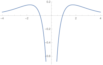
Figure 1: Typical shape of the potential $\mathfrak{w}$ given in (3.8)

The question of the convergence of the series (3.5) boils down to accessing to the leading in $N$ asymptotics of $\ln\big{|}\mathcal{Z}_{N}(x,t)\big{|}$. The multiple integral representation (3.6) for $\mathcal{Z}_{N}(x,t)$ is not in a form that would allows for an estimation of the leading large-$N$ behaviour of $\ln\big{|}\mathcal{Z}_{N}(x,t)\big{|}$, at least within the existing techniques. However, building on the representation (2.37) one may obtain an upper bound for $\big{|}\mathcal{Z}_{N}(x,t)\big{|}$ in terms of another $N$-fold multiple integral whose large-$N$ behaviour may be already accessed within the techniques that were pioneered in [4] and further developed so as to encompass $N$-dependent interactions in [12]. This bound is established below and constitutes the main result of this section.

Proposition 3.1.

Let $|x|>|t|$ and $p_{n}^{(\mathcal{O}_{k})}$ be bounded as in (1.5). Then, the $N^{\mathrm{th}}$ summand in the form factor expansion admits the upper bound

$$\big{|}\mathcal{Z}_{N}(m\mathfrak{r})\big{|}\;\leq\;\big{(}C\ln N\big{)}^{N}\cdot\mathrm{max}_{p\in[\![\,0\,;\,N\,]\!]}\big{|}\mathscr{Z}_{N,p}\big{(}\tfrac{m\mathfrak{r}}{2}\big{)}\big{|}\>,$$ (3.14)

where $C>0$ is some constant and

$$\mathscr{Z}_{N,p}(\varkappa)\,=\,\bigg{(}{\mathchoice{\dfrac{1}{\ln N}}{\dfrac{1}{\ln N}}{\frac{1}{\ln N}}{\frac{1}{\ln N}}}\bigg{)}^{N}\int\limits_{\mathbb{R}^{p}}\mathrm{d}^{p}\nu\int\limits_{\mathbb{R}^{N-p}}\mathrm{d}^{N-p}\lambda\prod\limits_{a=1}^{p}\Big{\{}\mathrm{e}^{-\varkappa\cosh(\nu_{a})}\Big{\}}\cdot\prod\limits_{a=1}^{N-p}\Big{\{}\mathrm{e}^{-\varkappa\cosh(\lambda_{a})}\Big{\}}\cdot\prod\limits_{a<b}^{p}\Big{\{}\mathrm{e}^{\mathfrak{w}(\nu_{ab})}\Big{\}}\\ \times\prod\limits_{a<b}^{N-p}\Big{\{}\mathrm{e}^{\mathfrak{w}(\lambda_{ab})}\Big{\}}\cdot\prod\limits_{a=1}^{p}\prod\limits_{b=1}^{N-p}\bigg{\{}\mathrm{e}^{\mathfrak{w}(\nu_{a}-\lambda_{b})}\prod\limits_{\epsilon=\pm}{\mathchoice{\dfrac{\sinh\big{[}\nu_{a}-\lambda_{b}-2\mathrm{i}\pi\epsilon\mathfrak{b}\big{]}}{\sinh(\nu_{a}-\lambda_{b})}}{\dfrac{\sinh\big{[}\nu_{a}-\lambda_{b}-2\mathrm{i}\pi\epsilon\mathfrak{b}\big{]}}{\sinh(\nu_{a}-\lambda_{b})}}{\frac{\sinh\big{[}\nu_{a}-\lambda_{b}-2\mathrm{i}\pi\epsilon\mathfrak{b}\big{]}}{\sinh(\nu_{a}-\lambda_{b})}}{\frac{\sinh\big{[}\nu_{a}-\lambda_{b}-2\mathrm{i}\pi\epsilon\mathfrak{b}\big{]}}{\sinh(\nu_{a}-\lambda_{b})}}}\bigg{\}}\;.$$ (3.15)

Proof —

Indeed, by using the obvious bound

$$\Big{|}\sum\limits_{k=1}^{p}a_{k}\Big{|}^{2}\,\leq\,p^{2}\sum\limits_{k=1}^{p}|a_{k}|^{2}$$ (3.16)

and the upper bound (1.5), one gets

$$\Big{|}\mathcal{K}_{N}^{(\mathcal{O}_{1})}(\boldsymbol{\beta}_{N})\cdot\mathcal{K}_{N}^{(\mathcal{O}_{2})}(\boldsymbol{\beta}_{N})\Big{|}\;\leq\;\bigg{(}2\,C_{1}\bigg{)}^{2N}\prod\limits_{a=1}^{N}\mathrm{e}^{2C_{2}|\beta_{a}|^{k}}\cdot\sum\limits_{\boldsymbol{\ell}_{N}\in\{0,1\}^{N}}\prod\limits_{a<b}^{N}\bigg{\{}{\mathchoice{\dfrac{\sinh\big{[}\beta_{ab}-2\mathrm{i}\pi\mathfrak{b}\ell_{ab}\big{]}\cdot\sinh\big{[}\beta_{ab}+2\mathrm{i}\pi\mathfrak{b}\ell_{ab}\big{]}}{\sinh^{2}(\beta_{ab})}}{\dfrac{\sinh\big{[}\beta_{ab}-2\mathrm{i}\pi\mathfrak{b}\ell_{ab}\big{]}\cdot\sinh\big{[}\beta_{ab}+2\mathrm{i}\pi\mathfrak{b}\ell_{ab}\big{]}}{\sinh^{2}(\beta_{ab})}}{\frac{\sinh\big{[}\beta_{ab}-2\mathrm{i}\pi\mathfrak{b}\ell_{ab}\big{]}\cdot\sinh\big{[}\beta_{ab}+2\mathrm{i}\pi\mathfrak{b}\ell_{ab}\big{]}}{\sinh^{2}(\beta_{ab})}}{\frac{\sinh\big{[}\beta_{ab}-2\mathrm{i}\pi\mathfrak{b}\ell_{ab}\big{]}\cdot\sinh\big{[}\beta_{ab}+2\mathrm{i}\pi\mathfrak{b}\ell_{ab}\big{]}}{\sinh^{2}(\beta_{ab})}}}\bigg{\}}\;.$$ (3.17)

Here, we stress that the summands ocurring in (3.17) are all real.

Observe that the summand appearing above is clearly symmetric in $\boldsymbol{\beta}_{N}$. Furthermore, for any $\boldsymbol{\ell}_{N}\in\{0,1\}^{N}$, there exists $p\in[\![\,1\,;\,N\,]\!]$ and $\sigma\in\mathfrak{S}_{N}$ such that

$$\ell_{\sigma(a)}=0\quad\mathrm{for}\quad a=1,\dots,p\qquad\mathrm{and}\qquad\ell_{\sigma(a)}=1\quad\mathrm{for}\quad a=p+1,\dots,N\;.$$ (3.18)

Hence, for this $\boldsymbol{\ell}_{N}$, it holds

$$\prod\limits_{a<b}^{N}\prod\limits_{\epsilon=\pm}\bigg{\{}{\mathchoice{\dfrac{\sinh\big{[}\beta_{ab}-2\mathrm{i}\pi\epsilon\mathfrak{b}\ell_{ab}\big{]}}{\sinh(\beta_{ab})}}{\dfrac{\sinh\big{[}\beta_{ab}-2\mathrm{i}\pi\epsilon\mathfrak{b}\ell_{ab}\big{]}}{\sinh(\beta_{ab})}}{\frac{\sinh\big{[}\beta_{ab}-2\mathrm{i}\pi\epsilon\mathfrak{b}\ell_{ab}\big{]}}{\sinh(\beta_{ab})}}{\frac{\sinh\big{[}\beta_{ab}-2\mathrm{i}\pi\epsilon\mathfrak{b}\ell_{ab}\big{]}}{\sinh(\beta_{ab})}}}\bigg{\}}\;=\;\prod\limits_{a=1}^{p}\prod\limits_{b=1+p}^{N}\prod\limits_{\epsilon=\pm}\bigg{\{}{\mathchoice{\dfrac{\sinh\big{[}\beta_{\sigma(a)\sigma(b)}+2\mathrm{i}\pi\epsilon\mathfrak{b}\big{]}}{\sinh(\beta_{\sigma(a)\sigma(b)})}}{\dfrac{\sinh\big{[}\beta_{\sigma(a)\sigma(b)}+2\mathrm{i}\pi\epsilon\mathfrak{b}\big{]}}{\sinh(\beta_{\sigma(a)\sigma(b)})}}{\frac{\sinh\big{[}\beta_{\sigma(a)\sigma(b)}+2\mathrm{i}\pi\epsilon\mathfrak{b}\big{]}}{\sinh(\beta_{\sigma(a)\sigma(b)})}}{\frac{\sinh\big{[}\beta_{\sigma(a)\sigma(b)}+2\mathrm{i}\pi\epsilon\mathfrak{b}\big{]}}{\sinh(\beta_{\sigma(a)\sigma(b)})}}}\bigg{\}}\;.$$ (3.19)

There are $C_{N}^{p}$ different choices of vectors $\boldsymbol{\ell}_{N}\in\{0,1\}^{N}$ having exactly $p$ entries equal to $0$ and for each such choice one may change variables under the integral

$$\beta_{\sigma(a)}\,=\,\nu_{a}\,,\;a=1,\dots,p,\quad\mathrm{and}\quad\beta_{\sigma(a)}\,=\,\lambda_{a-p}\,,\;a=p+1,\dots,N\,,$$ (3.20)

in which $\sigma$ is the associated permutation. Thus, upon using that

$$\mathrm{e}^{C_{2}|\beta|^{k}}\;\leq\;C^{\prime}\cdot\mathrm{e}^{{\mathchoice{\dfrac{m\mathfrak{r}}{2}}{\dfrac{m\mathfrak{r}}{2}}{\frac{m\mathfrak{r}}{2}}{\frac{m\mathfrak{r}}{2}}}\cosh(\beta)}$$ (3.21)

one gets the below upper bound valid for some $C>0$

$$\big{|}\mathcal{Z}_{N}(m\mathfrak{r})\big{|}\;\leq\;\bigg{(}C{\mathchoice{\dfrac{\ln N}{2}}{\dfrac{\ln N}{2}}{\frac{\ln N}{2}}{\frac{\ln N}{2}}}\bigg{)}^{N}\sum\limits_{p=0}^{N}C_{N}^{p}\mathscr{Z}_{N,p}\big{(}\tfrac{m\mathfrak{r}}{2}\big{)}$$ (3.22)

where $\mathscr{Z}_{N,p}(\varkappa)$ is as defined in (3.15). Then, since $\sum\limits_{p=0}^{N}C_{N}^{p}=2^{N}$, one gets the sought upper bound (3.14).  

Thus, in order to get a bound on the large-$N$ behaviour of $\big{|}\mathcal{Z}_{N}(m\mathfrak{r})\big{|}$, one should access to the leading one of $\ln\mathscr{Z}_{N,p}\big{(}\tfrac{m\mathfrak{r}}{2}\big{)}$, uniformly in $p\in[\![\,0\,;\,N\,]\!]$. One may expect, and this will be comforted by the analysis to come, that the leading in $N$ behaviour will be grasped, analogously to the random matrix setting [2, 12], from a concentration of measure property. To set the latter one should first identify the scale in $N$ at which the integration variables reach an equilibrium. The latter results from the compensation of the confining effect between the $\cosh$ potential and the repulsive, on short distances, effect of the potential $\mathfrak{w}$, all this balanced by the two-body interaction between the $\nu$ and $\lambda$ integration variables. One may heuristically convince oneself that the appropriate scale is reached upon dilating all variables by

$$\tau_{N}=\ln N\,.$$ (3.23)

This observation will be made rigorous and legitimate by the analysis to come.

Thus, I recast

$$\mathscr{Z}_{N,p}(\varkappa)\,=\,\int\limits_{\mathbb{R}^{N-p}}\mathrm{d}^{N-p}\lambda\int\limits_{\mathbb{R}^{p}}\mathrm{d}^{p}\nu\;\overline{\varrho}_{N,p}\big{(}\boldsymbol{\lambda}_{N-p},\boldsymbol{\nu}_{p}\big{)}$$ (3.24)

where the integrand takes the form

$$\overline{\varrho}_{N,p}\big{(}\boldsymbol{\lambda}_{N-p},\boldsymbol{\nu}_{p}\big{)}\;=\;\prod\limits_{a=1}^{p}\Big{\{}\mathrm{e}^{-V_{N}(\nu_{a})}\Big{\}}\cdot\prod\limits_{a=1}^{N-p}\Big{\{}\mathrm{e}^{-V_{N}(\lambda_{a})}\Big{\}}\\ \times\prod\limits_{a<b}^{p}\Big{\{}\mathrm{e}^{\mathfrak{w}_{N}(\nu_{ab})}\Big{\}}\cdot\prod\limits_{a<b}^{N-p}\Big{\{}\mathrm{e}^{\mathfrak{w}_{N}(\lambda_{ab})}\Big{\}}\cdot\prod\limits_{a=1}^{p}\prod\limits_{b=1}^{N-p}\bigg{\{}\mathrm{e}^{\mathfrak{w}_{\mathrm{tot};N}(\nu_{a}-\lambda_{b})}\bigg{\}}\;.$$ (3.25)

The product form of the integrand involves the functions

$$V_{N}(\lambda)\,=\,\varkappa\cosh(\tau_{N}\lambda)\quad,\quad\mathfrak{w}_{N}(\lambda)\,=\,\mathfrak{w}(\tau_{N}\lambda)\quad,\quad\mathfrak{w}_{\mathrm{tot};N}(\lambda)\,=\,\mathfrak{w}_{\mathrm{tot}}(\tau_{N}\lambda)\;,$$ (3.26)

upon agreeing that

$$\mathfrak{w}_{\mathrm{tot}}(\lambda)\,=\,\mathfrak{w}(\lambda)\,+\,\mathfrak{v}_{2\pi\mathfrak{b},0^{+}}(\lambda)\qquad\mathrm{with}\qquad\mathfrak{v}_{\alpha,\eta}(\lambda)\,=\,\ln\Bigg{(}{\mathchoice{\dfrac{\sinh(\lambda+\mathrm{i}\alpha)\cdot\sinh(\lambda-\mathrm{i}\alpha)}{\sinh(\lambda+\mathrm{i}\eta)\cdot\sinh(\lambda-\mathrm{i}\eta)}}{\dfrac{\sinh(\lambda+\mathrm{i}\alpha)\cdot\sinh(\lambda-\mathrm{i}\alpha)}{\sinh(\lambda+\mathrm{i}\eta)\cdot\sinh(\lambda-\mathrm{i}\eta)}}{\frac{\sinh(\lambda+\mathrm{i}\alpha)\cdot\sinh(\lambda-\mathrm{i}\alpha)}{\sinh(\lambda+\mathrm{i}\eta)\cdot\sinh(\lambda-\mathrm{i}\eta)}}{\frac{\sinh(\lambda+\mathrm{i}\alpha)\cdot\sinh(\lambda-\mathrm{i}\alpha)}{\sinh(\lambda+\mathrm{i}\eta)\cdot\sinh(\lambda-\mathrm{i}\eta)}}}\Bigg{)}\;.$$ (3.27)

In particular, it follows from the asymptotic expansion (3.9)-(3.10) that $\mathfrak{w}_{\mathrm{tot}}$ is bounded Lipschitz on $\mathbb{R}$.

Note that

$$\varrho_{N,p}\big{(}\boldsymbol{\lambda}_{N-p},\boldsymbol{\nu}_{p}\big{)}\;=\;{\mathchoice{\dfrac{\overline{\varrho}_{N,p}\big{(}\boldsymbol{\lambda}_{N-p},\boldsymbol{\nu}_{p}\big{)}}{\mathscr{Z}_{N,p}(\varkappa)}}{\dfrac{\overline{\varrho}_{N,p}\big{(}\boldsymbol{\lambda}_{N-p},\boldsymbol{\nu}_{p}\big{)}}{\mathscr{Z}_{N,p}(\varkappa)}}{\frac{\overline{\varrho}_{N,p}\big{(}\boldsymbol{\lambda}_{N-p},\boldsymbol{\nu}_{p}\big{)}}{\mathscr{Z}_{N,p}(\varkappa)}}{\frac{\overline{\varrho}_{N,p}\big{(}\boldsymbol{\lambda}_{N-p},\boldsymbol{\nu}_{p}\big{)}}{\mathscr{Z}_{N,p}(\varkappa)}}}\;,$$ (3.28)

gives rise to the density of a probability measure on $\mathbb{R}^{N-p}\times\mathbb{R}^{p}$.

4 Leading large-$N$ behaviour of $\mathscr{Z}_{N,p}(\varkappa)$ in terms of a minimisation problem

In this section, I obtain an upper bound on the leading order of the exponential large-$N$ asymptotics of the bounding partition function $\mathscr{Z}_{N,p}(\varkappa)$. Prior to stating the theorem, I need to introduce an auxiliary functional on $\mathcal{M}^{1}(\mathbb{R})\times\mathcal{M}^{1}(\mathbb{R})$, with $\mathcal{M}^{1}(\mathbb{R})$ referring to the space of probability measures on $\mathbb{R}$:

$$\mathcal{E}_{N,t}[\mu,\nu]\;=\;{\mathchoice{\dfrac{1}{N}}{\dfrac{1}{N}}{\frac{1}{N}}{\frac{1}{N}}}\bigg{\{}t\int\limits V_{N}(s)\mathrm{d}\nu(s)\,+\,(1-t)\int\limits V_{N}(s)\mathrm{d}\mu(s)\bigg{\}}\;-\;{\mathchoice{\dfrac{t^{2}}{2}}{\dfrac{t^{2}}{2}}{\frac{t^{2}}{2}}{\frac{t^{2}}{2}}}\int\limits\mathfrak{w}_{N}(s-u)\cdot\mathrm{d}\nu(s)\mathrm{d}\nu(u)\\ \;-\;{\mathchoice{\dfrac{(1-t)^{2}}{2}}{\dfrac{(1-t)^{2}}{2}}{\frac{(1-t)^{2}}{2}}{\frac{(1-t)^{2}}{2}}}\int\limits\mathfrak{w}_{N}(s-u)\cdot\mathrm{d}\mu(s)\mathrm{d}\mu(u)\,-\,t(1-t)\int\limits\mathfrak{w}_{\mathrm{tot};N}(s-u)\cdot\mathrm{d}\mu(s)\mathrm{d}\nu(u)\;.$$ (4.1)

The parameters $N\in\mathbb{N}^{*}$ and $t\in[0\,;1]$ appearing above should be considered as fixed in the minimisation problem to come. Note that for $t=0$, resp. $t=1$, $\mathcal{E}_{N,t}$ only depends on one of its two variables and hence effectively induces a functional only on $\mathcal{M}^{1}(\mathbb{R})$. Below, I will refer to $\mathcal{E}_{N,t}$, $0<t<1$, or to its effective restrictions to $\mathcal{M}^{1}(\mathbb{R})$, as "energy functional".

Theorem 4.1.

The multiple integral (3.24) admits the below estimate:

$$\mathscr{Z}_{N,p}(\varkappa)\,\leq\,\exp\bigg{\{}-N^{2}\mathrm{inf}\Big{\{}\,\mathcal{E}_{N,\frac{p}{N}}[\mu,\nu]\;:\;(\mu,\nu)\in\mathcal{M}^{1}(\mathbb{R})\times\mathcal{M}^{1}(\mathbb{R})\Big{\}}\;+\;\mathrm{O}\Big{(}N\tau_{N}^{2}\Big{)}\bigg{\}}\,,$$ (4.2)

in which the control is uniform in $p\in[\![\,0\,;\,N\,]\!]$.

Note that since $V_{N}$, $-\mathfrak{w}$ and $-\mathfrak{w}_{\mathrm{tot}}$ are all bounded from below, $\mathcal{E}_{N,t}[\mu,\nu]$ is bounded from below on $\mathcal{M}^{1}(\mathbb{R})\times\mathcal{M}^{1}(\mathbb{R})$ and so the infimum appearing in (4.2) is also bounded from below. The proof of the characterisation of the large-$N$ behaviour of $\mathscr{Z}_{N,p}(\varkappa)$ through a minimisation problem goes in two steps. First, one introduces $\overline{\mu}_{N,p}$ the measure on $\mathbb{R}^{N-p}\times\mathbb{R}^{p}$ induced by $\overline{\varrho}_{N,p}\big{(}\boldsymbol{\lambda}_{N-p},\boldsymbol{\nu}_{p}\big{)}$ given in (3.25) and shows that it concentrates with super-Gaussian precision on the interval $[-2+\epsilon\,;2+\epsilon]^{N}$. Then, one builds on this result to get an upper bound on $\mathscr{Z}_{N,p}(\varkappa)$. The techniques allowing one to establish such results are rather standard nowadays, see e.g. [2, 12].

In fact, I have little doubt that the upper bound in (4.2) is optimal, viz. that the inequality $\leq$ can be replaced by an $=$. However, following [2, 12], proving this equality would demand to obtain a lower bound on $\mathscr{Z}_{N,p}(\varkappa)$ by estimating the contribution to the integral (3.24) issuing from integration variables located in the vicinity of the configuration whose empirical measure is sufficiently close to the minimiser in (4.2). For this, one needs to have some quantitative information on the minimier’s density. While posing no conceptual problem to be obtained, doing so would demand much more work than what will be developed in Sections 6-9 relatively to solving a simpler minimisation problem which is already enough in what concerns the main goal of this work, viz. establishing the convergence of the form factor series. Hence, I omit establishing the lower-bound here.

4.1 Concentration on compact subsets

Lemma 4.2.

Let $\overline{\mu}_{N,p}$ be the measure on $\mathbb{R}^{N-p}times\mathbb{R}^{p}$ with density $\overline{\varrho}_{N,p}$ given by (3.25) and let $\epsilon>0$. Then, the partition function $\mathscr{Z}_{N,p}(\varkappa)$ enjoys the estimates

$$\mathscr{Z}_{N,p}(\varkappa)\,=\,\overline{\mu}_{N,p}\big{[}\Omega^{(\epsilon)}\big{]}\;+\;\mathrm{O}\Big{(}\mathrm{e}^{-{\mathchoice{\dfrac{\varkappa}{4}}{\dfrac{\varkappa}{4}}{\frac{\varkappa}{4}}{\frac{\varkappa}{4}}}N^{2+\epsilon}}\Big{)}\;,$$ (4.3)

where

$$\Omega^{(\epsilon)}\;=\;\Big{\{}(\boldsymbol{\lambda}_{N-p},\boldsymbol{\nu}_{p})\in\mathbb{R}^{N}\;:\;|\lambda_{a}|<2+\epsilon\;,\;\;a=1,\dots,N-p\quad and\quad|\nu_{a}|<2+\epsilon\;,\;\;a=1,\dots,p\Big{\}}$$ (4.4)

and $\overline{\mu}_{N,p}$ refers to the measure on $\mathbb{R}^{N-p}\times\mathbb{R}^{p}$ with density $\overline{\varrho}_{N,p}\big{(}\boldsymbol{\lambda}_{N-p},\boldsymbol{\nu}_{p}\big{)}$ introduced in (3.25).

Proof —  Given $a\in[\![\,1\,;\,N-p\,]\!]$ and $b\in[\![\,1\,;\,p\,]\!]$, let

$$O_{1;a}^{(\epsilon)}\;=\;\Big{\{}(\boldsymbol{\lambda}_{N-p},\boldsymbol{\nu}_{p})\in\mathbb{R}^{N}\;:\;|\lambda_{a}|\,\geq\,2+\epsilon\Big{\}}\quad\mathrm{and}\quad O_{2;b}^{(\epsilon)}\;=\;\Big{\{}(\boldsymbol{\lambda}_{N-p},\boldsymbol{\nu}_{p})\in\mathbb{R}^{N}\;:\;|\nu_{b}|\,\geq\,2+\epsilon\Big{\}}\;.$$ (4.5)

Then, since

$$\Big{[}\Omega^{(\epsilon)}\Big{]}^{\mathrm{c}}\subseteq\Big{\{}\bigcup\limits_{a=1}^{N-p}O_{1;a}^{(\epsilon)}\Big{\}}\,\bigcup\,\Big{\{}\bigcup\limits_{a=1}^{p}O_{2;a}^{(\epsilon)}\Big{\}}\;,$$ (4.6)

it follows that

$$\overline{\mu}_{N,p}\Big{[}\,\big{[}\Omega^{(\epsilon)}\big{]}^{\mathrm{c}}\,\Big{]}\;\leq\;\sum\limits_{a=1}^{N-p}\overline{\mu}_{N,p}\Big{[}O_{1;a}^{(\epsilon)}\Big{]}\,+\,\sum\limits_{a=1}^{p}\overline{\mu}_{N,p}\Big{[}O_{2;a}^{(\epsilon)}\Big{]}\;.$$ (4.7)

By using that $\mathfrak{w}$ is bounded from above, one gets

$$\overline{\mu}_{N,p}\Big{[}\,O_{k;a}^{(\epsilon)}\,\Big{]}\;\leq\;\exp\Bigg{\{}\frac{1}{2}\Big{[}p(p-1)\,+\,(N-p)(N-p-1)\Big{]}\sup_{\mathbb{R}}\{\mathfrak{w}(\lambda)\}\;+\;p(N-p)||\mathfrak{w}_{\mathrm{tot}}||_{L^{\infty}(\mathbb{R})}\Bigg{\}}\\ \times\bigg{(}\int\limits_{\mathbb{R}}\mathrm{d}s\,\mathrm{e}^{-V_{N}(s)}\bigg{)}^{N-1}\cdot\int\limits_{|s|>2+\epsilon}\mathrm{d}s\,\mathrm{e}^{-V_{N}(s)}\\ \;\leq\;{\mathchoice{\dfrac{\exp\Big{\{}cN^{2}\Big{\}}}{\tau_{N}^{N-1}}}{\dfrac{\exp\Big{\{}cN^{2}\Big{\}}}{\tau_{N}^{N-1}}}{\frac{\exp\Big{\{}cN^{2}\Big{\}}}{\tau_{N}^{N-1}}}{\frac{\exp\Big{\{}cN^{2}\Big{\}}}{\tau_{N}^{N-1}}}}\cdot\bigg{(}\int\limits_{\mathbb{R}}\mathrm{d}s\,\mathrm{e}^{-V(s)}\bigg{)}^{N-1}\cdot 2\,\mathrm{e}^{-V_{N}(2+\epsilon)}\cdot\int\limits_{2+\epsilon}^{+\infty}\mathrm{d}s\,\mathrm{e}^{-(s-2-\epsilon)V_{N}^{\prime}(2+\epsilon)}\\ \;\leq\;\exp\Big{\{}c^{\prime}N^{2}\Big{\}}\cdot\exp\Big{\{}-\varkappa\cosh[\tau_{N}(2+\epsilon)]\Big{\}}\;\leq\;{\mathchoice{\dfrac{C^{\prime\prime}}{N}}{\dfrac{C^{\prime\prime}}{N}}{\frac{C^{\prime\prime}}{N}}{\frac{C^{\prime\prime}}{N}}}\mathrm{e}^{-{\mathchoice{\dfrac{\varkappa}{4}}{\dfrac{\varkappa}{4}}{\frac{\varkappa}{4}}{\frac{\varkappa}{4}}}N^{2+\epsilon}}\;,$$ (4.8)

for some $N$-independent constants $c,c^{\prime},C^{\prime\prime}>0$. Also, in the intermediate steps I used that

$$\cosh(x)\,=\,\sum\limits_{n\geq 0}{\mathchoice{\dfrac{\cosh^{(n)}(y)}{n!}}{\dfrac{\cosh^{(n)}(y)}{n!}}{\frac{\cosh^{(n)}(y)}{n!}}{\frac{\cosh^{(n)}(y)}{n!}}}\cdot(x-y)^{n}\;\geq\;\cosh(y)\,+\,(x-y)\sinh(y)$$ (4.9)

which holds provided that $x\geq y\geq 0$.  

4.2 Upper bound

Lemma 4.3.

One has the uniform in $p\in[\![\,0\,;\,N\,]\!]$ upper bound

$$\mathscr{Z}_{N,p}(\varkappa)\;\leq\;\exp\bigg{\{}-N^{2}\mathrm{inf}\Big{\{}\,\mathcal{E}_{N,\frac{p}{N}}[\mu,\nu]\;:\;(\mu,\nu)\in\mathcal{M}^{1}(\mathbb{R})\times\mathcal{M}^{1}(\mathbb{R})\Big{\}}\;+\;\mathrm{O}\Big{(}N\tau_{N}^{2}\Big{)}\bigg{\}}\;.$$ (4.10)

Proof —

To start with, one introduces a regularised vector $\widetilde{\boldsymbol{\beta}}_{\ell}\in\mathbb{R}^{\ell}$ associated with any vector $\boldsymbol{\beta}_{\ell}\in\mathbb{R}^{\ell}$. Namely, given $\beta_{1}\leq\dots\leq\beta_{\ell}$, define $\widetilde{\beta}_{1}<\dots<\widetilde{\beta}_{\ell}$ as

$$\widetilde{\beta}_{1}\,=\,\beta_{1}\quad\mathrm{and}\quad\widetilde{\beta}_{k+1}\,=\,\widetilde{\beta}_{k}\,+\,\max\big{(}\,\beta_{k+1}-\beta_{k},\mathrm{e}^{-\tau_{N}^{2}}\big{)}\,.$$ (4.11)

For any $\boldsymbol{\beta}_{\ell}\in\mathbb{R}^{\ell}$, one picks $\sigma\in\mathfrak{S}_{\ell}$, such that $\beta_{\sigma(1)}\leq\dots\leq\beta_{\sigma(\ell)}$ and then obtains $\widetilde{\beta}_{1}^{\,(\sigma)}<\dots<\widetilde{\beta}_{\ell}^{\,(\sigma)}$ by the above procedure. Then, the vector $\widetilde{\boldsymbol{\beta}}_{\ell}\in\mathbb{R}^{\ell}$ has coordinates $\big{(}\widetilde{\boldsymbol{\beta}}_{\ell}\big{)}_{k}\,=\,\widetilde{\beta}_{\sigma^{-1}(k)}^{\,(\sigma)}$. The new configuration has been constructed such that, for $\ell\not=k$,

$$\big{|}\widetilde{\beta}_{k}-\widetilde{\beta}_{\ell}\big{|}\,\geq\,\mathrm{e}^{-\tau_{N}^{2}}\qquad,\quad\big{|}\beta_{k}-\beta_{\ell}\big{|}\,\leq\,\big{|}\widetilde{\beta}_{k}-\widetilde{\beta}_{\ell}\big{|}\quad\mathrm{and}\quad\big{|}\beta_{k}-\widetilde{\beta}_{k}\big{|}\leq(\sigma^{-1}(k)-1)\cdot\mathrm{e}^{-\tau_{N}^{2}}\,\leq\,(N-1)\mathrm{e}^{-\tau_{N}^{2}}\;,$$ (4.12)

with $\sigma$ as introduced above. Here, the main point is that, as such, the variables $\widetilde{\beta}_{k}$ exhibit much better spacing properties than the original ones, while still remaining close to the original variables $\beta_{k}$. Note that the scale of regularisation $\mathrm{e}^{-\tau_{N}^{2}}$ is somewhat arbitrary, but in any case should be taken negligible compared to an algebraic decay.

To proceed further, one needs to introduce the empirical measure associated with an $\ell$-dimensional vector $\boldsymbol{\nu}_{\ell}\in\mathbb{R}^{\ell}$ :

$$L_{\ell}^{(\boldsymbol{\nu})}={\mathchoice{\dfrac{1}{\ell}}{\dfrac{1}{\ell}}{\frac{1}{\ell}}{\frac{1}{\ell}}}\sum_{a=1}^{\ell}\delta_{\nu_{a}}$$

where $\delta_{x}$ refers to the Dirac mass at $x$. Further, denote by $L_{\ell;u}^{(\boldsymbol{\nu})}$ the convolution of $L_{\ell}^{(\boldsymbol{\nu})}$ with the uniform probability measure on $[0\,;\tfrac{1}{N}\mathrm{e}^{-\tau_{N}^{2}}]$. The main advantage of the convoluted empirical measure $L_{\ell;u}^{(\boldsymbol{\nu})}$ is that it is Lebesgue continuous, this for any $\boldsymbol{\nu}_{\ell}\in\mathbb{R}^{\ell}$; as such it can appear in the argument of $\mathcal{E}_{N,\frac{p}{N}}$ and yield finite results.

By using the empirical measures associated with $\boldsymbol{\lambda}_{N-p}$ and $\boldsymbol{\nu}_{p}$, one may recast the unnormalised integrand $\overline{\varrho}_{N,p}$ introduced in (3.25),

$$\overline{\varrho}_{N,p}\big{(}\boldsymbol{\lambda}_{N-p},\boldsymbol{\nu}_{p}\big{)}\,=\,\exp\Bigg{\{}-p\int\limits V_{N}(s)\mathrm{d}L_{p}^{(\boldsymbol{\nu})}(s)\,-\,(N-p)\int\limits V_{N}(s)\mathrm{d}L_{N-p}^{(\boldsymbol{\lambda})}(s)\,+\,{\mathchoice{\dfrac{p^{2}}{2}}{\dfrac{p^{2}}{2}}{\frac{p^{2}}{2}}{\frac{p^{2}}{2}}}\int\limits_{x\not=y}\mathfrak{w}_{N}(x-y)\mathrm{d}L_{p}^{(\boldsymbol{\nu})}(x)\mathrm{d}L_{p}^{(\boldsymbol{\nu})}(y)\\ \,+\,{\mathchoice{\dfrac{(N-p)^{2}}{2}}{\dfrac{(N-p)^{2}}{2}}{\frac{(N-p)^{2}}{2}}{\frac{(N-p)^{2}}{2}}}\int\limits_{x\not=y}\mathfrak{w}_{N}(x-y)\mathrm{d}L_{N-p}^{(\boldsymbol{\lambda})}(x)\mathrm{d}L_{N-p}^{(\boldsymbol{\lambda})}(y)\,+\,p(N-p)\int\limits\mathfrak{w}_{\mathrm{tot};N}(x-y)\mathrm{d}L_{p}^{(\boldsymbol{\nu})}(x)\mathrm{d}L_{N-p}^{(\boldsymbol{\lambda})}(y)\Bigg{\}}$$ (4.13)

To get an upper bound on $\mathscr{Z}_{N,p}(\varkappa)$ one needs to relate this expression, up to some controllable errors, to an evaluation of the energy functional $\mathcal{E}_{N,{\mathchoice{\dfrac{p}{N}}{\dfrac{p}{N}}{\frac{p}{N}}{\frac{p}{N}}}}$ on some well-built convoluted empirical measure. Following Lemma 4.2, one may limit the reasoning to integration variables belonging to $[-2-\epsilon\,;2+\epsilon]$ for some $\epsilon>0$.

Pick $\boldsymbol{\nu}_{p}\in[-2-\epsilon\,;2+\epsilon]^{p}$ with $p\in[\![\,1\,;\,N\,]\!]$. Further, set $w_{p;a}^{(\sigma)}=\Big{[}(\sigma^{-1}(a)-1)+\tfrac{1}{N}\Big{]}\mathrm{e}^{-\tau_{N}^{2}}$ with $\sigma\in\mathfrak{S}_{p}$ such that $\nu_{\sigma(1)}\leq\cdots\leq\nu_{\sigma(p)}$ and observe that

$$\Big{|}\nu_{a}\,-\,\widetilde{\nu}_{a}\,-\,\tfrac{\mathrm{e}^{-\tau_{N}^{2}}}{N}s\Big{|}\;\leq\;w_{p;a}^{(\sigma)}\quad\mathrm{when}\quad s\in[0\,;1]\;.$$ (4.14)

Then, by the mean value theorem, one gets the bound

$$\bigg{|}\int\limits V_{N}(s)\mathrm{d}L_{p}^{(\boldsymbol{\nu})}(s)\,-\,\int\limits V_{N}(s)\mathrm{d}L_{p;u}^{(\,\widetilde{\boldsymbol{\nu}}\,)}(s)\bigg{|}\;\leq\;{\mathchoice{\dfrac{1}{p}}{\dfrac{1}{p}}{\frac{1}{p}}{\frac{1}{p}}}\sum\limits_{a=1}^{p}\int\limits_{0}^{1}\!\mathrm{d}s\,\Big{|}V_{N}(\nu_{a})\,-\,V_{N}\Big{(}\widetilde{\nu}_{a}\,+\,\tfrac{\mathrm{e}^{-\tau_{N}^{2}}}{N}s\Big{)}\Big{|}\\ \leq\;{\mathchoice{\dfrac{1}{p}}{\dfrac{1}{p}}{\frac{1}{p}}{\frac{1}{p}}}\sum\limits_{a=1}^{p}w_{N;a}^{(\sigma)}\cdot\underset{t\in[0\,;1]}{\mathrm{sup}}\bigg{\{}\varkappa\tau_{N}\Big{|}\sinh\Big{(}\tau_{N}[\nu_{a}+tw_{p;a}^{(\sigma)}]\Big{)}\Big{|}\bigg{\}}\;\leq\;p\tau_{N}C^{\prime}N^{2+\epsilon}\mathrm{e}^{-\tau_{N}^{2}}\;,$$ (4.15)

for some $C^{\prime}>0$ and where we used that $w_{p;a}^{(\sigma)}\,\leq p\mathrm{e}^{-\tau_{N}^{2}}$ and that, for $|\nu|\leq 2+\epsilon$, it holds

$$\big{|}\sinh\big{[}\tau_{N}(\nu+N\mathrm{e}^{-\tau_{N}^{2}})\big{]}\big{|}\;\sim\;{\mathchoice{\dfrac{N^{2+\epsilon}}{2}}{\dfrac{N^{2+\epsilon}}{2}}{\frac{N^{2+\epsilon}}{2}}{\frac{N^{2+\epsilon}}{2}}}\;.$$ (4.16)

Likewise, using similar bounds and the fact that $\mathfrak{w}_{\mathrm{tot}}$ is bounded Lipschitz, one gets

$$\bigg{|}\int\limits\mathfrak{w}_{\mathrm{tot};N}(x-y)\,\mathrm{d}L_{p}^{(\boldsymbol{\nu})}(x)\mathrm{d}L_{N-p}^{(\boldsymbol{\lambda})}(y)\,-\,\int\limits\mathfrak{w}_{\mathrm{tot};N}(x-y)\,\mathrm{d}L_{p;u}^{(\,\widetilde{\boldsymbol{\nu}}\,)}(x)\mathrm{d}L_{N-p;u}^{(\,\widetilde{\boldsymbol{\lambda}}\,)}(y)\bigg{|}\\ \;\leq\;{\mathchoice{\dfrac{1}{p(N-p)}}{\dfrac{1}{p(N-p)}}{\frac{1}{p(N-p)}}{\frac{1}{p(N-p)}}}\sum\limits_{a=1}^{p}\sum\limits_{b=1}^{N-p}\int\limits_{0}^{1}\!\mathrm{d}s\mathrm{d}u\bigg{|}\mathfrak{w}_{\mathrm{tot};N}(\nu_{a}-\lambda_{b})\,-\,\mathfrak{w}_{\mathrm{tot};N}\Big{(}\widetilde{\nu}_{a}-\widetilde{\lambda}_{b}\,+\,\tfrac{\mathrm{e}^{-\tau_{N}^{2}}}{N}(s-u)\Big{)}\Big{|}\\ \leq\;{\mathchoice{\dfrac{1}{p(N-p)}}{\dfrac{1}{p(N-p)}}{\frac{1}{p(N-p)}}{\frac{1}{p(N-p)}}}\sum\limits_{a=1}^{p}\sum\limits_{b=1}^{N-p}\tau_{N}||\mathfrak{w}_{\mathrm{tot}}^{\prime}||_{L^{\infty}(\mathbb{R})}\Big{\{}p-1+N-p-1+\tfrac{1}{N}\Big{\}}\mathrm{e}^{-\tau_{N}^{2}}\;\leq\;CN\tau_{N}\mathrm{e}^{-\tau_{N}^{2}}\;,$$ (4.17)

for some $C>0$.

Finally, the estimate on the integrals involving the $\mathfrak{w}_{N}$ interaction require more care due to the presence of a logarithmic behaviour at the origin: $\mathfrak{w}(\lambda)\,=\,2\ln|\lambda|\,+\,\mathfrak{w}_{\mathrm{reg}}(\lambda)$, with $\mathfrak{w}_{\mathrm{reg}}$ analytic in some open neighbourhood of $0$, c.f. (3.9). This upper bound is obtained in two steps, depending one whether $|\nu_{a}-\nu_{b}|$ is small enough or not.

(i) If $|\nu_{a}-\nu_{b}|\,\leq\,\epsilon/\tau_{N}$ then, by using that $\lambda\mapsto\ln\lambda$ is increasing on $\mathbb{R}^{+}$ and the shorthand notation $\nu_{ab}=\nu_{a}-\nu_{b}$, one has for $N$-large enough

$$\mathfrak{w}_{N}(\nu_{ab})\;\leq\;2\ln\big{(}\tau_{N}|\,\widetilde{\nu}_{ab}|\big{)}\,+\,\mathfrak{w}_{\mathrm{reg};N}\big{(}\,\widetilde{\nu}_{ab}\big{)}\;+\;\Big{(}|\nu_{a}-\widetilde{\nu}_{a}|\,+\,|\nu_{b}-\widetilde{\nu}_{b}|\Big{)}\cdot\tau_{N}\cdot\underset{s\in[0\,;1]}{\mathrm{sup}}\bigg{|}\mathfrak{w}_{\mathrm{reg}}^{\prime}\Big{(}\tau_{N}(\,\widetilde{\nu}_{ab}+s[\nu_{ab}\,-\,\widetilde{\nu}_{ab}])\Big{)}\bigg{|}\\ \;\leq\;\mathfrak{w}_{N}(\,\widetilde{\nu}_{ab})\,+\,2\tau_{N}\,(p-1)\,||\mathfrak{w}_{\mathrm{reg}}^{\prime}||_{L^{\infty}([-2\epsilon\,;2\epsilon])}\cdot\mathrm{e}^{-\tau_{N}^{2}}\;.$$ (4.18)

(ii) If $|\nu_{a}-\nu_{b}|\,\geq\,\epsilon/\tau_{N}$ then it holds

$$\mathfrak{w}_{N}(\nu_{ab})\;\leq\;\mathfrak{w}_{N}\big{(}\,\widetilde{\nu}_{ab}\big{)}\;+\;\Big{(}|\nu_{a}-\widetilde{\nu}_{a}|\,+\,|\nu_{b}-\widetilde{\nu}_{b}|\Big{)}\cdot\tau_{N}\cdot\underset{s\in[0\,;1]}{\mathrm{sup}}\bigg{\{}\mathfrak{w}^{\prime}\Big{(}\tau_{N}(\,\widetilde{\nu}_{ab}+s[\nu_{ab}\,-\,\widetilde{\nu}_{ab}])\Big{)}\bigg{\}}\\ \;\leq\;\mathfrak{w}_{N}(\,\widetilde{\nu}_{ab})\,+\,2\tau_{N}\,(p-1)\,||\mathfrak{w}^{\prime}||_{L^{\infty}(\mathbb{R}\setminus[-\frac{\epsilon}{2}\,;\frac{\epsilon}{2}])}\cdot\mathrm{e}^{-\tau_{N}^{2}}\;.$$ (4.19)

This leads to the upper bound

$$\int\limits_{x\not=y}\mathfrak{w}_{N}(x-y)\,\mathrm{d}L_{p}^{(\boldsymbol{\nu})}(x)\mathrm{d}L_{p}^{(\boldsymbol{\nu})}(y)\,-\,\int\limits_{x\not=y}\mathfrak{w}_{N}(x-y)\,\mathrm{d}L_{p}^{(\,\widetilde{\boldsymbol{\nu}}\,)}(x)\mathrm{d}L_{p}^{(\,\widetilde{\boldsymbol{\nu}}\,)}(y)\;\leq\;C\,p\,\tau_{N}\,\mathrm{e}^{-\tau_{N}^{2}}\;,$$ (4.20)

in which $C>0$ is an $\epsilon$-dependent constant. Further, one has that

$$\delta\Sigma\;=\;\int\limits_{x\not=y}\mathfrak{w}_{N}(x-y)\,\mathrm{d}L_{p}^{(\,\widetilde{\boldsymbol{\nu}}\,)}(x)\mathrm{d}L_{p}^{(\,\widetilde{\boldsymbol{\nu}}\,)}(y)\,-\,\int\limits_{x\not=y}\mathfrak{w}_{N}(x-y)\,\mathrm{d}L_{p;u}^{(\,\widetilde{\boldsymbol{\nu}}\,)}(x)\mathrm{d}L_{p;u}^{(\,\widetilde{\boldsymbol{\nu}}\,)}(y)\\ \;=\;\int\limits_{x\not=y}\mathrm{d}L_{p}^{(\,\widetilde{\boldsymbol{\nu}}\,)}(x)\mathrm{d}L_{p}^{(\,\widetilde{\boldsymbol{\nu}}\,)}(y)\int\limits_{0}^{1}\mathrm{d}s\mathrm{d}u\bigg{\{}\mathfrak{w}_{N}(x-y)\,-\,\mathfrak{w}_{N}\Big{(}x-y\,+\,\tfrac{\mathrm{e}^{-\tau_{N}^{2}}}{N}(s-u)\Big{)}\bigg{\}}\;-\;{\mathchoice{\dfrac{1}{p}}{\dfrac{1}{p}}{\frac{1}{p}}{\frac{1}{p}}}\int\limits_{0}^{1}\mathrm{d}s\mathrm{d}u\mathfrak{w}_{N}\Big{(}\tfrac{\mathrm{e}^{-\tau_{N}^{2}}}{N}(s-u)\Big{)}\;.$$ (4.21)

Then, using the expressions

$$\mathfrak{w}_{N}(x)\,=\,\left\{\begin{array}[]{ccc}2\ln(\tau_{N}|x|)\,+\,\mathfrak{w}_{\mathrm{reg};N}(x)&\mathrm{for}&|x|\leq\epsilon/\tau_{N}\vspace{2mm}\\ \mathfrak{w}(\tau_{N}x)&\mathrm{for}&|x|\geq\epsilon/\tau_{N}\end{array}\right.$$ (4.22)

one gets the upper bound

$$\Big{|}\mathfrak{w}_{N}(x)\,-\,\mathfrak{w}_{N}(y)\Big{|}\leq C\bigg{(}1+\underset{t\in[0\,;1]}{\mathrm{max}}{\mathchoice{\dfrac{1}{|x+t(y-x)|}}{\dfrac{1}{|x+t(y-x)|}}{\frac{1}{|x+t(y-x)|}}{\frac{1}{|x+t(y-x)|}}}\bigg{)}\cdot|x-y|\;,$$ (4.23)

which leads, for any $|x-y|\geq\mathrm{e}^{-\tau_{N}^{2}}$ and $s,u\in[0\,;1]$, to

$$\bigg{|}\mathfrak{w}_{N}(x-y)\,-\,\mathfrak{w}_{N}\Big{(}x-y\,+\,\tfrac{\mathrm{e}^{-\tau_{N}^{2}}}{N}(s-u)\Big{)}\bigg{|}\;\leq\;{\mathchoice{\dfrac{C}{N}}{\dfrac{C}{N}}{\frac{C}{N}}{\frac{C}{N}}}|s-u|\;.$$ (4.24)

Hence, all-in-all, taking into account (4.12), $\big{|}\delta\Sigma\big{|}\,=\,\mathrm{O}\Big{(}\tfrac{\tau_{N}^{2}}{p}\Big{)}$, where the control issues from the last term in (4.21).

Thus, upon invoking Lemma 4.2, one gets that, for some constant $C>0$ and with $\Omega^{(\epsilon)}$ as introduced in (4.4),

$$\mathscr{Z}_{N,p}(\varkappa)\;\leq\;\mathrm{O}\Big{(}\mathrm{e}^{-{\mathchoice{\dfrac{\varkappa}{4}}{\dfrac{\varkappa}{4}}{\frac{\varkappa}{4}}{\frac{\varkappa}{4}}}N^{2+\epsilon}}\Big{)}\;+\;\int\limits_{\Omega^{(\epsilon)}}\mathrm{d}^{p}\nu\mathrm{d}^{N-p}\lambda\\ \exp\bigg{\{}-\int\limits V_{N}(s)\Big{[}p\mathrm{d}L_{p;u}^{(\,\widetilde{\boldsymbol{\nu}}\,)}(s)\,+\,(N-p)\mathrm{d}L_{N-p;u}^{(\,\widetilde{\boldsymbol{\lambda}}\,)}(s)\Big{]}+C\tau_{N}\mathrm{e}^{-\tau_{N}^{2}}N^{2+\epsilon}\Big{(}p^{2}+(N-p)^{2}\Big{)}\bigg{\}}\\ \times\exp\bigg{\{}p(N-p)\int\limits\mathfrak{w}_{\mathrm{tot};N}(x-y)\,\mathrm{d}L_{p;u}^{(\,\widetilde{\boldsymbol{\nu}}\,)}(x)\mathrm{d}L_{N-p;u}^{(\,\widetilde{\boldsymbol{\lambda}}\,)}(y)\;+\;Cp(N-p)N\tau_{N}\mathrm{e}^{-\tau_{N}^{2}}\bigg{\}}\\ \times\exp\bigg{\{}\tfrac{1}{2}\int\limits\mathfrak{w}_{N}(x-y)\Big{[}p^{2}\mathrm{d}L_{p;u}^{(\,\widetilde{\boldsymbol{\nu}}\,)}(x)\mathrm{d}L_{p;u}^{(\,\widetilde{\boldsymbol{\nu}}\,)}(y)\,+\,(N-p)^{2}\mathrm{d}L_{N-p;u}^{(\,\widetilde{\boldsymbol{\lambda}}\,)}(x)\mathrm{d}L_{N-p;u}^{(\,\widetilde{\boldsymbol{\lambda}}\,)}(y)\Big{]}\\ \;+\;C\big{[}p^{3}+(N-p)^{3}\big{]}\tau_{N}\mathrm{e}^{-\tau_{N}^{2}}\;+\;C\big{[}p+(N-p)\big{]}\tau_{N}^{2}\bigg{\}}\;.$$ (4.25)

Thus, one gets

$$\mathscr{Z}_{N,p}(\varkappa)\;=\;\mathrm{O}\Big{(}\mathrm{e}^{-{\mathchoice{\dfrac{\varkappa}{4}}{\dfrac{\varkappa}{4}}{\frac{\varkappa}{4}}{\frac{\varkappa}{4}}}N^{2+\epsilon}}\Big{)}\;+\;\int\limits_{\Omega^{(\epsilon)}}\mathrm{d}^{p}\nu\mathrm{d}^{N-p}\lambda\exp\bigg{\{}-N^{2}\mathcal{E}_{N,\frac{p}{N}}\Big{[}L_{N-p;u}^{(\,\widetilde{\boldsymbol{\lambda}}\,)}\,,\,L_{p;u}^{(\,\widetilde{\boldsymbol{\nu}}\,)}\Big{]}\;+\;\mathrm{O}\Big{(}N\tau_{N}^{2}\Big{)}\bigg{\}}\\ \;\leq\;\Big{(}4+2\epsilon\Big{)}^{N}\cdot\exp\bigg{\{}-N^{2}\mathrm{inf}\Big{\{}\,\mathcal{E}_{N,\frac{p}{N}}[\mu,\nu]\;:\;(\mu,\nu)\in\mathcal{M}^{1}(\mathbb{R})\times\mathcal{M}^{1}(\mathbb{R})\Big{\}}\;+\;\mathrm{O}\Big{(}N\tau_{N}^{2}\Big{)}\bigg{\}}\;+\;\mathrm{O}\Big{(}\mathrm{e}^{-{\mathchoice{\dfrac{\varkappa}{4}}{\dfrac{\varkappa}{4}}{\frac{\varkappa}{4}}{\frac{\varkappa}{4}}}N^{2+\epsilon}}\Big{)}\\ \;\leq\;\exp\bigg{\{}-N^{2}\mathrm{inf}\Big{\{}\,\mathcal{E}_{N,\frac{p}{N}}[\mu,\nu]\;:\;(\mu,\nu)\in\mathcal{M}^{1}(\mathbb{R})\times\mathcal{M}^{1}(\mathbb{R})\Big{\}}\;+\;\mathrm{O}\Big{(}N\tau_{N}^{2}\Big{)}\bigg{\}}\;+\;\mathrm{O}\Big{(}\mathrm{e}^{-{\mathchoice{\dfrac{\varkappa}{4}}{\dfrac{\varkappa}{4}}{\frac{\varkappa}{4}}{\frac{\varkappa}{4}}}N^{2+\epsilon}}\Big{)}\;.$$ (4.26)

To get the claim, it is enough to get a Gaussian lower bound on the partition $\mathscr{Z}_{N,p}(\varkappa)$ what can be done by using Jensen’s inequality applied to the probability measure on $\mathbb{R}^{N}$:

$$\mathrm{d}\mathfrak{p}_{N}\,=\,\prod\limits_{a=1}^{N-p}\Big{\{}\mathrm{d}\lambda_{a}\;\mathrm{e}^{-V_{N}(\lambda_{a})}\Big{\}}\cdot\prod\limits_{a=1}^{p}\Big{\{}\mathrm{d}\nu_{a}\;\mathrm{e}^{-V_{N}(\nu_{a})}\Big{\}}\cdot\bigg{\{}\int\limits_{\mathbb{R}}\mathrm{d}s\mathrm{e}^{-V_{N}(s)}\bigg{\}}^{-N}$$ (4.27)

what yields

$$\mathscr{Z}_{N,p}(\varkappa)\;\geq\;\exp\Bigg{\{}\int\limits_{\mathbb{R}^{N}}\mathrm{d}\mathfrak{p}_{N}\bigg{(}\sum\limits_{a<b}^{N-p}\mathfrak{w}_{N}(\lambda_{ab})\,+\,\sum\limits_{a<b}^{p}\mathfrak{w}_{N}(\nu_{ab})\,+\,\sum\limits_{a=1}^{p}\sum\limits_{b=1}^{N-p}\mathfrak{w}_{N;\mathrm{tot}}(\nu_{a}-\lambda_{b})\bigg{)}\Bigg{\}}\cdot\bigg{\{}\int\limits_{\mathbb{R}}\mathrm{d}s\mathrm{e}^{-V_{N}(s)}\bigg{\}}^{N}\\ \;\geq\;\exp\Bigg{\{}-N^{2}\int\limits_{\mathbb{R}^{2}}{\mathchoice{\dfrac{\mathrm{d}s\mathrm{d}u\,\mathrm{e}^{-V(s)-V(u)}}{\Big{(}\int\limits_{\mathbb{R}}\mathrm{d}x\,\mathrm{e}^{-V(x)}\Big{)}^{2}}}{\dfrac{\mathrm{d}s\mathrm{d}u\,\mathrm{e}^{-V(s)-V(u)}}{\Big{(}\int\limits_{\mathbb{R}}\mathrm{d}x\,\mathrm{e}^{-V(x)}\Big{)}^{2}}}{\frac{\mathrm{d}s\mathrm{d}u\,\mathrm{e}^{-V(s)-V(u)}}{\Big{(}\int\limits_{\mathbb{R}}\mathrm{d}x\,\mathrm{e}^{-V(x)}\Big{)}^{2}}}{\frac{\mathrm{d}s\mathrm{d}u\,\mathrm{e}^{-V(s)-V(u)}}{\Big{(}\int\limits_{\mathbb{R}}\mathrm{d}x\,\mathrm{e}^{-V(x)}\Big{)}^{2}}}}\cdot\Big{[}\,|\mathfrak{w}(s-u)|\,+\,|\mathfrak{w}_{\mathrm{tot}}(s-u)|\Big{]}\Bigg{\}}\cdot\bigg{\{}\int\limits_{\mathbb{R}}{\mathchoice{\dfrac{\mathrm{d}s}{\tau_{N}}}{\dfrac{\mathrm{d}s}{\tau_{N}}}{\frac{\mathrm{d}s}{\tau_{N}}}{\frac{\mathrm{d}s}{\tau_{N}}}}\mathrm{e}^{-V(s)}\bigg{\}}^{N}\;\geq\;\mathrm{e}^{-cN^{2}}\;.$$ (4.28)

Hence, it holds that

$$\mathscr{Z}_{N,p}(\varkappa)\cdot\bigg{(}1\,-\,\mathrm{O}\Big{(}{\mathchoice{\dfrac{\mathrm{e}^{-{\mathchoice{\dfrac{\varkappa}{4}}{\dfrac{\varkappa}{4}}{\frac{\varkappa}{4}}{\frac{\varkappa}{4}}}N^{2+\epsilon}}}{\mathscr{Z}_{N,p}(\varkappa)}}{\dfrac{\mathrm{e}^{-{\mathchoice{\dfrac{\varkappa}{4}}{\dfrac{\varkappa}{4}}{\frac{\varkappa}{4}}{\frac{\varkappa}{4}}}N^{2+\epsilon}}}{\mathscr{Z}_{N,p}(\varkappa)}}{\frac{\mathrm{e}^{-{\mathchoice{\dfrac{\varkappa}{4}}{\dfrac{\varkappa}{4}}{\frac{\varkappa}{4}}{\frac{\varkappa}{4}}}N^{2+\epsilon}}}{\mathscr{Z}_{N,p}(\varkappa)}}{\frac{\mathrm{e}^{-{\mathchoice{\dfrac{\varkappa}{4}}{\dfrac{\varkappa}{4}}{\frac{\varkappa}{4}}{\frac{\varkappa}{4}}}N^{2+\epsilon}}}{\mathscr{Z}_{N,p}(\varkappa)}}}\Big{)}\bigg{)}\;\leq\;\exp\bigg{\{}-N^{2}\mathrm{inf}\Big{\{}\,\mathcal{E}_{N,\frac{p}{N}}[\mu,\nu]\;:\;(\mu,\nu)\in\mathcal{M}^{1}(\mathbb{R})\times\mathcal{M}^{1}(\mathbb{R})\Big{\}}\;+\;\mathrm{O}\Big{(}N\tau_{N}^{2}\Big{)}\bigg{\}}$$ (4.29)

what leads to the claim since

$$\ln\bigg{(}1\,-\,\mathrm{O}\Big{(}\mathscr{Z}_{N,p}^{-1}(\varkappa)\cdot\mathrm{e}^{-{\mathchoice{\dfrac{\varkappa}{4}}{\dfrac{\varkappa}{4}}{\frac{\varkappa}{4}}{\frac{\varkappa}{4}}}N^{2+\epsilon}}\Big{)}\bigg{)}\,=\,\mathrm{O}\Big{(}\mathrm{e}^{-{\mathchoice{\dfrac{\varkappa}{8}}{\dfrac{\varkappa}{8}}{\frac{\varkappa}{8}}{\frac{\varkappa}{8}}}N^{2+\epsilon}}\Big{)}$$ (4.30)

 

5 The energy functional associated with the bounding partition function

As shown in Theorem 4.1, the large-$N$ behaviour of $\mathscr{Z}_{N,p}(\varkappa)$ can be controlled, up to $\mathrm{O}(N\tau_{N}^{2})$ corrections, by solving the minimisation problem associated with the energy functional $\mathcal{E}_{N,t}$ on $\mathcal{M}^{1}(\mathbb{R})\times\mathcal{M}^{1}(\mathbb{R})$ introduced in (4.1). In this section, I will establish the unique solvability of this problem as well as a lower bound for the value of the minimum.

Proposition 5.1.

For any $0<t<1$, the functional $\mathcal{E}_{N,t}$ is lower semi-continuous on $\mathcal{M}^{1}(\mathbb{R})\times\mathcal{M}^{1}(\mathbb{R})$, has compact level sets, is not identically $+\infty$ and is bounded from below. The same properties hold for $\mathcal{E}_{N,0}$ and $\mathcal{E}_{N,1}$ seen as functionals on $\mathcal{M}^{1}(\mathbb{R})$.

Proof —  Let $0<t<1$. The functional $\mathcal{E}_{N,t}$ is lower semi-continuous as supremum of a family of continuous functionals in respect to the bounded-Lipschitz topology on $\mathcal{M}^{1}(\mathbb{R})\times\mathcal{M}^{1}(\mathbb{R})$: $\mathcal{E}_{N,t}[\mu,\nu]=\mathrm{sup}_{M\nearrow+\infty}\mathcal{E}_{N,t}^{(M)}[\mu,\nu]$ with

$$\mathcal{E}_{N,t}^{(M)}[\mu,\nu]\;=\;{\mathchoice{\dfrac{1}{N}}{\dfrac{1}{N}}{\frac{1}{N}}{\frac{1}{N}}}\int\limits_{\mathbb{R}}\mathrm{min}\big{(}V_{N}(s),M)\cdot\Big{\{}t\mathrm{d}\nu(s)\,+\,(1-t)\mathrm{d}\mu(s)\Big{\}}\;+\;{\mathchoice{\dfrac{t^{2}}{2}}{\dfrac{t^{2}}{2}}{\frac{t^{2}}{2}}{\frac{t^{2}}{2}}}\int\limits_{\mathbb{R}^{2}}\mathrm{min}\big{(}-\mathfrak{w}_{N}(s-u),M\big{)}\cdot\mathrm{d}\nu(s)\mathrm{d}\nu(u)\\ \;+\;{\mathchoice{\dfrac{(1-t)^{2}}{2}}{\dfrac{(1-t)^{2}}{2}}{\frac{(1-t)^{2}}{2}}{\frac{(1-t)^{2}}{2}}}\int\limits_{\mathbb{R}^{2}}\mathrm{min}\big{(}-\mathfrak{w}_{N}(s-u),M\big{)}\cdot\mathrm{d}\mu(s)\mathrm{d}\mu(u)\,-\,t(1-t)\int\limits_{\mathbb{R}^{2}}\mathfrak{w}_{\mathrm{tot};N}(s-u)\cdot\mathrm{d}\mu(s)\mathrm{d}\nu(u)\;,$$ (5.1)

where we used that $\lambda\mapsto\mathfrak{w}_{\mathrm{tot};N}(\lambda)$ is already bounded Lipschitz on $\mathbb{R}$. Further, $\mathcal{E}_{N,t}$ is not identically $+\infty$ as follows from evaluating it on the probability measures

$$(\mathrm{d}\mu(s),\mathrm{d}\nu(s))\,=\,(\psi(s)\cdot\mathrm{d}s,\psi(s)\cdot\mathrm{d}s)\quad\mathrm{with}\quad\psi\in\mathcal{C}^{\infty}_{\mathrm{c}}(\mathbb{R})\quad\mathrm{such}\,\mathrm{that}\quad\int\limits_{\mathbb{R}}\psi(s)\mathrm{d}s=1\;.$$ (5.2)

Let

$$f_{t}(s,u)={\mathchoice{\dfrac{t}{2N}}{\dfrac{t}{2N}}{\frac{t}{2N}}{\frac{t}{2N}}}\Big{(}V_{N}(s)\,+\,V_{N}(u)\Big{)}\,-\,{\mathchoice{\dfrac{t^{2}}{2}}{\dfrac{t^{2}}{2}}{\frac{t^{2}}{2}}{\frac{t^{2}}{2}}}\mathfrak{w}_{N}(s-u)\;.$$ (5.3)

Clearly, $f_{t}$ is bounded from below on $\mathbb{R}^{2}$. Denote by $c_{t}$ a lower bound on it, viz. $f_{t}\geq c_{t}$. Owing to $||\mathfrak{w}_{\mathrm{tot}}||_{L^{\infty}(\mathbb{R})}$ being finite, the existence of a lower bound on $f$ entails that $\mathcal{E}_{N,t}$ is bounded from below as

$$\mathcal{E}_{N,t}[\mu,\nu]\geq c_{t}+c_{1-t}\,-\,t(1-t)||\mathfrak{w}_{\mathrm{tot}}||_{L^{\infty}(\mathbb{R})}\;.$$ (5.4)

It remains to establish that $\mathcal{E}_{N,t}$ has compact level sets. For that purpose, first observe that $f_{t}$ blows up

• at $\infty$ due to the exponential blow up of $V_{N}$,

• along the diagonal due to the logarithmic singularity of $\mathfrak{w}_{N}$.

Hence, there exists $K_{L}\rightarrow+\infty$ such that

$$\Big{\{}(s,u)\,:\,f_{t}(s,u)\geq K_{L}\;\;\mathrm{and}\;\;f_{1-t}(s,u)\geq K_{L}\Big{\}}\supset B_{L}=\Big{\{}(s,u)\,:\,|s|>L\;\;\mathrm{or}\;\;|u|>L\Big{\}}\cup\Big{\{}(s,u)\,:\,|s-u|<L^{-1}\Big{\}}\;.$$ (5.5)

Let $M>0$ and $(\mu,\nu)$ be such that $\mathcal{E}_{N,t}[\mu,\nu]\leq M$. Then, for $L$ large enough, it holds

$$\big{(}\mu\big{[}\mathbb{R}\setminus[-L\,;L]\big{]}\big{)}^{2}\,+\,\big{(}\nu\big{[}\mathbb{R}\setminus[-L\,;L]\big{]}\big{)}^{2}\;\leq\;\mu\otimes\mu\Big{[}\big{\{}(s,u)\,:\,f_{1-t}(s,u)\geq K_{L}\big{\}}\Big{]}\,+\,\nu\otimes\nu\Big{[}\big{\{}(s,u)\,:\,f_{t}(s,u)\geq K_{L}\big{\}}\Big{]}\;.$$ (5.6)

Observe that owing to $K_{L}-c_{1-t}>0$ for $L$ large enough and $c_{1-t}$ being a lower bound for $f_{1-t}(s,u)$ one gets the lower bounds

$${\mathchoice{\dfrac{f_{1-t}(s,u)-c_{1-t}}{K_{L}-c_{1-t}}}{\dfrac{f_{1-t}(s,u)-c_{1-t}}{K_{L}-c_{1-t}}}{\frac{f_{1-t}(s,u)-c_{1-t}}{K_{L}-c_{1-t}}}{\frac{f_{1-t}(s,u)-c_{1-t}}{K_{L}-c_{1-t}}}}\;\geq\;1\quad\mathrm{on}\quad\Big{\{}(s,u)\,:\,f_{1-t}(s,u)\geq K_{L}\Big{\}}\quad\mathrm{and}\quad{\mathchoice{\dfrac{f_{1-t}(s,u)-c_{1-t}}{K_{L}-c_{1-t}}}{\dfrac{f_{1-t}(s,u)-c_{1-t}}{K_{L}-c_{1-t}}}{\frac{f_{1-t}(s,u)-c_{1-t}}{K_{L}-c_{1-t}}}{\frac{f_{1-t}(s,u)-c_{1-t}}{K_{L}-c_{1-t}}}}\;\geq\;0\quad\mathrm{on}\quad\mathbb{R}^{2}$$ (5.7)

Hence, it holds that

$$\big{(}\mu\big{[}\mathbb{R}\setminus[-L\,;L]\big{]}\big{)}^{2}\;\leq\;\int\limits_{\big{\{}(s,u)\,:\,f_{1-t}(s,u)\geq K_{L}\big{\}}}\mathrm{d}\mu(s)\mathrm{d}\mu(u)\;\leq\;\int\limits_{\big{\{}(s,u)\,:\,f_{1-t}(s,u)\geq K_{L}\big{\}}}\mathrm{d}\mu(s)\mathrm{d}\mu(u){\mathchoice{\dfrac{f_{1-t}(s,u)-c_{1-t}}{K_{L}-c_{1-t}}}{\dfrac{f_{1-t}(s,u)-c_{1-t}}{K_{L}-c_{1-t}}}{\frac{f_{1-t}(s,u)-c_{1-t}}{K_{L}-c_{1-t}}}{\frac{f_{1-t}(s,u)-c_{1-t}}{K_{L}-c_{1-t}}}}\;\leq\;\int\limits_{\mathbb{R}^{2}}\mathrm{d}\mu(s)\mathrm{d}\mu(u){\mathchoice{\dfrac{f_{1-t}(s,u)-c_{1-t}}{K_{L}-c_{1-t}}}{\dfrac{f_{1-t}(s,u)-c_{1-t}}{K_{L}-c_{1-t}}}{\frac{f_{1-t}(s,u)-c_{1-t}}{K_{L}-c_{1-t}}}{\frac{f_{1-t}(s,u)-c_{1-t}}{K_{L}-c_{1-t}}}}\;.$$ (5.8)

An analogous bound holds for $\nu$. From there it follows that

$$\big{(}\mu\big{[}\mathbb{R}\setminus[-L\,;L]\big{]}\big{)}^{2}\,+\,\big{(}\nu\big{[}\mathbb{R}\setminus[-L\,;L]\big{]}\big{)}^{2}\;\leq\;\int\limits_{\mathbb{R}^{2}}\mathrm{d}\mu(s)\mathrm{d}\mu(u)\,{\mathchoice{\dfrac{f_{1-t}(s,u)-c_{1-t}}{K_{L}-c_{1-t}}}{\dfrac{f_{1-t}(s,u)-c_{1-t}}{K_{L}-c_{1-t}}}{\frac{f_{1-t}(s,u)-c_{1-t}}{K_{L}-c_{1-t}}}{\frac{f_{1-t}(s,u)-c_{1-t}}{K_{L}-c_{1-t}}}}\;+\int\limits_{\mathbb{R}^{2}}\mathrm{d}\nu(s)\mathrm{d}\nu(u)\,{\mathchoice{\dfrac{f_{t}(s,u)-c_{t}}{K_{L}-c_{t}}}{\dfrac{f_{t}(s,u)-c_{t}}{K_{L}-c_{t}}}{\frac{f_{t}(s,u)-c_{t}}{K_{L}-c_{t}}}{\frac{f_{t}(s,u)-c_{t}}{K_{L}-c_{t}}}}\\ \;\leq\;{\mathchoice{\dfrac{1}{K_{L}-\mathrm{max}\big{\{}c_{t},c_{1-t}\big{\}}}}{\dfrac{1}{K_{L}-\mathrm{max}\big{\{}c_{t},c_{1-t}\big{\}}}}{\frac{1}{K_{L}-\mathrm{max}\big{\{}c_{t},c_{1-t}\big{\}}}}{\frac{1}{K_{L}-\mathrm{max}\big{\{}c_{t},c_{1-t}\big{\}}}}}\cdot\Big{\{}\mathcal{E}_{N,t}[\mu,\nu]\,-\,c_{t}\,-\,c_{1-t}+t(1-t)||\mathfrak{w}_{\mathrm{tot}}||_{L^{\infty}(\mathbb{R})}\Big{\}}\;\leq\;{\mathchoice{\dfrac{C_{M}}{K_{L}}}{\dfrac{C_{M}}{K_{L}}}{\frac{C_{M}}{K_{L}}}{\frac{C_{M}}{K_{L}}}}\;,$$ (5.9)

for some $C_{M}>0$ and $L>L_{0}$ with $L_{0}$ being $M$-independent and where $c_{t}$ is the lower bound on $f_{t}$. Hence,

$$(\mu,\nu)\in\mathcal{K}_{M}\times\mathcal{K}_{M}\qquad\mathrm{with}\qquad\mathcal{K}_{M}\;=\;\bigcap\limits_{\begin{subarray}{c}L\in\mathbb{N}\\ >L_{0}\end{subarray}}\bigg{\{}\mu\in\mathcal{M}^{1}(\mathbb{R})\,:\,\mu\big{[}\mathbb{R}\setminus[-L\,;L]\big{]}\,\leq\,\sqrt{\tfrac{C_{M}}{K_{L}}}\bigg{\}}\;.$$ (5.10)

Since $\mathcal{K}_{M}$ is uniformly tight by construction and closed as an intersection of level sets of the lower semi-continuous functions $\mu\mapsto\int\limits_{\mathbb{R}\setminus[-L\,;L]}\mathrm{d}\mu(s)$, by virtue of Prokhorov’s theorem, $\mathcal{K}_{M}$ is compact. Since the level sets of $\mathcal{E}_{N,t}$ are closed, (5.10) entails that they are compact as well.  

For further purpose, I introduce two functions

$$\mathfrak{w}_{N}^{(\pm)}(u)\;=\;\mathfrak{w}^{(\pm)}(\tau_{N}u)\qquad\mathrm{with}\qquad\left\{\begin{array}[]{ccc}\mathfrak{w}^{(+)}(u)&=&\mathfrak{w}(u)+{\mathchoice{\dfrac{1}{2}}{\dfrac{1}{2}}{\frac{1}{2}}{\frac{1}{2}}}\mathfrak{v}_{2\pi\mathfrak{b},0^{+}}(u)\\ \mathfrak{w}^{(-)}(u)&=&-{\mathchoice{\dfrac{1}{2}}{\dfrac{1}{2}}{\frac{1}{2}}{\frac{1}{2}}}\mathfrak{v}_{2\pi\mathfrak{b},0^{+}}(u)\end{array}\right.\;,$$ (5.11)

and where $\mathfrak{v}_{\alpha,\eta}$ has been introduced in (3.27).

Both $\mathfrak{w}^{(\pm)}$ have strictly negative Fourier transforms, namely

$$\mathfrak{w}^{(\upsilon)}(x)\,=\,-\int\limits_{\mathbb{R}}\mathrm{d}\lambda{\mathchoice{\dfrac{R^{(\upsilon)}(\lambda)}{\lambda}}{\dfrac{R^{(\upsilon)}(\lambda)}{\lambda}}{\frac{R^{(\upsilon)}(\lambda)}{\lambda}}{\frac{R^{(\upsilon)}(\lambda)}{\lambda}}}\,\mathrm{e}^{-\mathrm{i}\lambda x}\;,\quad x\not=0\,,$$ (5.12)

where the integration is to be understood in the sense of an oscillatory Riemann–integral, and where

$$R^{(+)}(\lambda)\;=\;{\mathchoice{\dfrac{\sinh(\pi\mathfrak{b}\lambda)\cdot\sinh(\pi\hat{\mathfrak{b}}\lambda)\cdot\sinh(\tfrac{\pi}{2}\lambda)}{\cosh^{2}(\tfrac{\pi}{2}\lambda)}}{\dfrac{\sinh(\pi\mathfrak{b}\lambda)\cdot\sinh(\pi\hat{\mathfrak{b}}\lambda)\cdot\sinh(\tfrac{\pi}{2}\lambda)}{\cosh^{2}(\tfrac{\pi}{2}\lambda)}}{\frac{\sinh(\pi\mathfrak{b}\lambda)\cdot\sinh(\pi\hat{\mathfrak{b}}\lambda)\cdot\sinh(\tfrac{\pi}{2}\lambda)}{\cosh^{2}(\tfrac{\pi}{2}\lambda)}}{\frac{\sinh(\pi\mathfrak{b}\lambda)\cdot\sinh(\pi\hat{\mathfrak{b}}\lambda)\cdot\sinh(\tfrac{\pi}{2}\lambda)}{\cosh^{2}(\tfrac{\pi}{2}\lambda)}}}\qquad\mathrm{and}\qquad R^{(-)}(\lambda)\;=\;{\mathchoice{\dfrac{\sinh(\pi\mathfrak{b}\lambda)\cdot\sinh(\pi\hat{\mathfrak{b}}\lambda)}{\sinh(\tfrac{\pi}{2}\lambda)}}{\dfrac{\sinh(\pi\mathfrak{b}\lambda)\cdot\sinh(\pi\hat{\mathfrak{b}}\lambda)}{\sinh(\tfrac{\pi}{2}\lambda)}}{\frac{\sinh(\pi\mathfrak{b}\lambda)\cdot\sinh(\pi\hat{\mathfrak{b}}\lambda)}{\sinh(\tfrac{\pi}{2}\lambda)}}{\frac{\sinh(\pi\mathfrak{b}\lambda)\cdot\sinh(\pi\hat{\mathfrak{b}}\lambda)}{\sinh(\tfrac{\pi}{2}\lambda)}}}\;.$$ (5.13)

The formulae for $R^{(\upsilon)}$ follow from the integral representation for $\mathfrak{w}$ given in (3.8) and the explicit form of the Fourier transform of the function $\mathfrak{v}_{\alpha,\eta}$ which was defined in (3.27):

$$\mathcal{F}\big{[}\mathfrak{v}_{\alpha,\eta}\big{]}(\lambda)\,=\,\int\limits_{\mathbb{R}}\mathrm{d}x\,\mathrm{e}^{\mathrm{i}x\lambda}\mathfrak{v}_{\alpha,\eta}(x)\,=\,-4\pi{\mathchoice{\dfrac{\sinh\Big{(}\lambda\tfrac{\eta-\alpha}{2}\Big{)}\sinh\Big{(}\lambda\tfrac{\pi-\eta-\alpha}{2}\Big{)}}{\lambda\sinh\Big{(}\tfrac{\pi\lambda}{2}\Big{)}}}{\dfrac{\sinh\Big{(}\lambda\tfrac{\eta-\alpha}{2}\Big{)}\sinh\Big{(}\lambda\tfrac{\pi-\eta-\alpha}{2}\Big{)}}{\lambda\sinh\Big{(}\tfrac{\pi\lambda}{2}\Big{)}}}{\frac{\sinh\Big{(}\lambda\tfrac{\eta-\alpha}{2}\Big{)}\sinh\Big{(}\lambda\tfrac{\pi-\eta-\alpha}{2}\Big{)}}{\lambda\sinh\Big{(}\tfrac{\pi\lambda}{2}\Big{)}}}{\frac{\sinh\Big{(}\lambda\tfrac{\eta-\alpha}{2}\Big{)}\sinh\Big{(}\lambda\tfrac{\pi-\eta-\alpha}{2}\Big{)}}{\lambda\sinh\Big{(}\tfrac{\pi\lambda}{2}\Big{)}}}}\;.$$ (5.14)

I refer to Lemma A.2 given in Appendix A for the details on how to get (5.14).

The functions $\mathfrak{w}^{(\pm)}$ give rise to the below two functionals

$$\mathcal{E}_{N}^{(+)}\big{[}\sigma\big{]} = {\mathchoice{\dfrac{1}{N}}{\dfrac{1}{N}}{\frac{1}{N}}{\frac{1}{N}}}\int\limits V_{N}(s)\,\mathrm{d}\sigma(s)\,-\,{\mathchoice{\dfrac{1}{2}}{\dfrac{1}{2}}{\frac{1}{2}}{\frac{1}{2}}}\int\limits\mathfrak{w}_{N}^{(+)}(s-u)\cdot\mathrm{d}\sigma(s)\,\mathrm{d}\sigma(u)\,,$$ (5.15)

$$\mathcal{E}_{N}^{(-)}\big{[}\sigma\big{]} = -{\mathchoice{\dfrac{1}{2}}{\dfrac{1}{2}}{\frac{1}{2}}{\frac{1}{2}}}\int\limits\mathfrak{w}_{N}^{(-)}(s-u)\cdot\mathrm{d}\sigma(s)\,\mathrm{d}\sigma(u)\;.$$ (5.16)

$\mathcal{E}_{N}^{(+)}$ is a functional on $\mathcal{M}^{1}(\mathbb{R})$ while $\mathcal{E}_{N}^{(-)}$ is a functional on $\mathcal{M}^{(2t-1)}_{\mathfrak{s}}(\mathbb{R})$, the space of signed, bounded, measures on $\mathbb{R}$ of total mass $2t-1$.

Lemma 5.2.

Let $0<t<1$. $\mathcal{E}_{N,t}$ is strictly convex and may be recast as

$$\mathcal{E}_{N,t}\big{[}\mu,\nu\big{]}\;=\;\sum\limits_{\upsilon=\pm}\mathcal{E}_{N}^{(\upsilon)}\big{[}\sigma^{(\upsilon)}_{t}\big{]}\qquad with\qquad\sigma^{(\pm)}_{t}\,=\,t\nu\pm(1-t)\mu\;.$$ (5.17)

Moreover, it holds

$$\mathcal{E}_{N,t}\big{[}\alpha\mu+(1-\alpha)\sigma,\alpha\nu+(1-\alpha)\varrho\big{]}\,-\,\alpha\mathcal{E}_{N,t}\big{[}\mu,\nu\big{]}\,-\,(1-\alpha)\mathcal{E}_{N,t}\big{[}\sigma,\varrho\big{]}\;=\;-\alpha(1-\alpha)\mathfrak{D}_{N,t}\big{[}\mu-\sigma,\nu-\varrho\big{]}$$ (5.18)

where

$$\mathfrak{D}_{N,t}\big{[}\mu,\nu\big{]}\;=\;-t(1-t)\int\limits_{\mathbb{R}^{2}}\mathfrak{w}_{\mathrm{tot};N}(s-u)\cdot\mathrm{d}\mu(s)\mathrm{d}\nu(u)\;-\;{\mathchoice{\dfrac{1}{2}}{\dfrac{1}{2}}{\frac{1}{2}}{\frac{1}{2}}}\int\limits_{\mathbb{R}^{2}}\mathfrak{w}_{N}(s-u)\cdot\Big{(}t^{2}\mathrm{d}\nu(s)\mathrm{d}\nu(u)\;+\;(1-t)^{2}\mathrm{d}\mu(s)\mathrm{d}\mu(u)\Big{)}\,\;.$$ (5.19)

For compactly supported signed measures of zero total mass, $\mathfrak{D}_{N,t}$ satisfies

$$\mathfrak{D}_{N,t}\big{[}\mu,\nu\big{]}\;\geq\;0\quad and\quad\mathfrak{D}_{N,t}\big{[}\mu,\nu\big{]}\,=\,0\quad if\,and\,only\,if\quad(\mu,\nu)=(0,0)\;.$$ (5.20)

Analogous statements hold, upon restricting to $\mathcal{M}^{1}(\mathbb{R})$, when $t=0$ or $t=1$.

Proof —  Equations (5.17)-(5.18) follows from straightforward calculations upon implementing in $\mathcal{E}_{N,t}$ the change of unknown measure given by (5.17). To establish the properties of $\mathfrak{D}_{N,t}$ and hence the strict convexity of $\mathcal{E}_{N,t}$, one implements the change of variables given in (5.17) so as to get, for any signed measure on $\mathbb{R}$ of zero mass, that

$$\mathfrak{D}_{N,t}\big{[}\mu,\nu\big{]}\;=\;-\,{\mathchoice{\dfrac{1}{2}}{\dfrac{1}{2}}{\frac{1}{2}}{\frac{1}{2}}}\int\limits_{\mathbb{R}^{2}}\mathfrak{w}_{N}^{(+)}(s-u)\cdot\mathrm{d}\sigma^{(+)}_{t}(s)\,\mathrm{d}\sigma^{(+)}_{t}(u)\,-\,{\mathchoice{\dfrac{1}{2}}{\dfrac{1}{2}}{\frac{1}{2}}{\frac{1}{2}}}\int\limits_{\mathbb{R}^{2}}\mathfrak{w}_{N}^{(-)}(s-u)\cdot\mathrm{d}\sigma^{(-)}_{t}(s)\,\mathrm{d}\sigma^{(-)}_{t}(u)\;.$$ (5.21)

Thus, one gets that

$$\mathfrak{D}_{N,t}\big{[}\mu,\nu\big{]}\;=\;{\mathchoice{\dfrac{1}{2}}{\dfrac{1}{2}}{\frac{1}{2}}{\frac{1}{2}}}\int\limits_{\mathbb{R}}\mathrm{d}\lambda\,\bigg{\{}\;\big{|}\mathcal{F}\big{[}\sigma^{(+)}_{t}\big{]}(\lambda)\big{|}^{2}{\mathchoice{\dfrac{R^{(+)}(\lambda)}{\lambda}}{\dfrac{R^{(+)}(\lambda)}{\lambda}}{\frac{R^{(+)}(\lambda)}{\lambda}}{\frac{R^{(+)}(\lambda)}{\lambda}}}\,+\,\big{|}\mathcal{F}\big{[}\sigma^{(-)}_{t}\big{]}(\lambda)\big{|}^{2}{\mathchoice{\dfrac{R^{(-)}(\lambda)}{\lambda}}{\dfrac{R^{(-)}(\lambda)}{\lambda}}{\frac{R^{(-)}(\lambda)}{\lambda}}{\frac{R^{(-)}(\lambda)}{\lambda}}}\bigg{\}}\;,$$ (5.22)

which is a number in $[0\,;+\infty]$ and where $\sigma_{t}^{(\pm)}$ are related to $\mu,\nu$ through (5.17). Here, I remind that the Fourier transform of a signed measure $\mu$ such that $|\mu|$ has finite total mass is expressed as

$$\mathcal{F}[\mu](\lambda)\;=\;\int\limits_{\mathbb{R}}\mathrm{d}\mu(s)\mathrm{e}^{\mathrm{i}s\lambda}\;.$$ (5.23)

Observe that if $\mu,\nu$ are signed, compactly supported, measures on $\mathbb{R}$ with zero total mass then for any $t\in[0\,;1]$, $\lambda\mapsto\mathcal{F}\big{[}\sigma^{(\upsilon)}_{t}\big{]}(\lambda)$ is entire.

Now, given two such measures, since

• $R^{(\pm)}(\lambda)/\lambda$ are both positive on $\mathbb{R}$,

• the only zero of $R^{(+)}(\lambda)/\lambda$ on $\mathbb{R}$ is at $\lambda=0$ and is double,

• $R^{(-)}(\lambda)/\lambda$ has no zeroes on $\mathbb{R}$,

it follows that if $\mathfrak{D}_{N,t}\big{[}\mu,\nu\big{]}\,=\,0$, then it holds

$$\mathcal{F}\big{[}\sigma^{(\upsilon)}_{t}\big{]}(\lambda)\;=\;0\quad\mathrm{on}\;\mathbb{R}^{*}\;.$$ (5.24)

However, since these are entire functions, it holds $\mathcal{F}\big{[}\sigma^{(\upsilon)}_{t}\big{]}=0$. This entails that $\sigma^{(\upsilon)}_{t}=0$ and thus, for $0<t<1$, that $\mu=\nu=0$.

The reasoning when $t=0$ or $t=1$ are quite analogous.  

Theorem 5.3.

For $0<t<1$ $\mathcal{E}_{N,t}$ admits a unique minimiser of $\mathcal{M}^{1}(\mathbb{R})\times\mathcal{M}^{1}(\mathbb{R})$. Similarly, $\mathcal{E}_{N,0}$ and $\mathcal{E}_{N,1}$ admit unique minimisers of $\mathcal{M}^{1}(\mathbb{R})$.

Proof —  $\mathcal{E}_{N,t}$ is lower-continuous with compact level-sets, bounded from below and not identically $+\infty$ by virtue of Proposition 5.1. Hence, it attains its minimum. Since it is strictly convex by virtue of Lemma 5.2, this minimum is unique.  

From now on, we will denote the unique minimiser for $0<t<1$ as $\big{(}\mu_{\mathrm{eq}}^{(N,t)},\nu_{\mathrm{eq}}^{(N,t)}\big{)}$, viz.

$$\mathrm{inf}\bigg{\{}\mathcal{E}_{N,t}[\mu,\nu]\;:\;(\mu,\nu)\in\mathcal{M}^{1}(\mathbb{R})\times\mathcal{M}^{1}(\mathbb{R})\bigg{\}}\;=\;\mathcal{E}_{N,t}\Big{[}\mu_{\mathrm{eq}}^{(N,t)},\nu_{\mathrm{eq}}^{(N,t)}\Big{]}\;.$$ (5.25)

By virtue of (5.17), the minimisation problem may thus be recast as

$$\mathcal{E}_{N,t}\Big{[}\mu_{\mathrm{eq}}^{(N,t)},\nu_{\mathrm{eq}}^{(N,t)}\Big{]}\;=\;\mathrm{inf}\left\{\sum\limits_{\upsilon=\pm}\mathcal{E}_{N}^{(\upsilon)}\big{[}\sigma^{(\upsilon)}\big{]}\;:\;\begin{array}[]{c}\big{(}\sigma^{(+)},\sigma^{(-)}\big{)}\in\mathcal{M}^{1}(\mathbb{R})\times\mathcal{M}^{(2t-1)}_{\mathfrak{s}}(\mathbb{R})\vspace{2mm}\\ \Big{(}\tfrac{\sigma^{(+)}+\sigma^{(-)}}{2t},\tfrac{\sigma^{(+)}-\sigma^{(-)}}{2(1-t)}\Big{)}\in\mathcal{M}^{1}(\mathbb{R})\times\mathcal{M}^{1}(\mathbb{R})\end{array}\right\}\;.$$ (5.26)

Above $\mathcal{M}^{(\alpha)}_{\mathfrak{s}}(\mathbb{R})$ stands for the space of real signed measures on $\mathbb{R}$ of total mass $\alpha\in\mathbb{R}$. The constraint appearing in the second line does not allow one, a priori, to reduce the two-dimensional vector equilibrium problem associated with $\mathcal{E}_{N,t}$ into two one-dimensional problems. However, (5.26) allows one to obtain a lower bound for $\mathcal{E}_{N,t}\big{[}\mu_{\mathrm{eq}}^{(N,t)},\nu_{\mathrm{eq}}^{(N,t)}\big{]}$ in terms of the minimum of $\mathcal{E}_{N}^{(+)}$ which can be characterised by solving a one-dimensional equilibrium problem. The estimates obtained by computing this minimum turn out to be enough for the purpose of this analysis. Indeed, it is readily seen that $\mathcal{E}_{N}^{(+)}$ is lower-continuous, has compact level sets, is strictly convex on $\mathcal{M}^{1}(\mathbb{R})$, bounded from below and not identically $+\infty$. Thus, there exists a unique probability measure $\sigma_{\mathrm{eq}}^{(N)}$ such that

$$\mathcal{E}_{N}^{(+)}\big{[}\sigma_{\mathrm{eq}}^{(N)}\big{]}\;=\;\mathrm{inf}\Big{\{}\mathcal{E}_{N}^{(+)}\big{[}\sigma\big{]}\;:\;\sigma\in\mathcal{M}^{1}(\mathbb{R})\Big{\}}\;.$$ (5.27)

Moreover, it follows from the positivity of $R^{(-)}(\lambda)/\lambda$ that, for any signed measure $\sigma$ on $\mathbb{R}$,

$$\mathcal{E}_{N}^{(-)}\big{[}\sigma\big{]}\;=\;{\mathchoice{\dfrac{1}{2}}{\dfrac{1}{2}}{\frac{1}{2}}{\frac{1}{2}}}\int\limits_{\mathbb{R}}\mathrm{d}\lambda\,\big{|}\mathcal{F}\big{[}\sigma\big{]}(\lambda)\big{|}^{2}{\mathchoice{\dfrac{R^{(-)}(\lambda)}{\lambda}}{\dfrac{R^{(-)}(\lambda)}{\lambda}}{\frac{R^{(-)}(\lambda)}{\lambda}}{\frac{R^{(-)}(\lambda)}{\lambda}}}\;\geq\;0\;.$$ (5.28)

As a consequence,

$$\mathcal{E}_{N,t}\Big{[}\mu_{\mathrm{eq}}^{(N,t)},\nu_{\mathrm{eq}}^{(N,t)}\Big{]}\;\geq\;\mathcal{E}_{N}^{(+)}\big{[}\sigma_{\mathrm{eq}}^{(N)}\big{]}\;.$$ (5.29)

Corollary 5.4.

One has the upper bound

$$\mathscr{Z}_{N,p}(\varkappa)\,\leq\,\exp\bigg{\{}-N^{2}\mathcal{E}_{N}^{(+)}\big{[}\sigma_{\mathrm{eq}}^{(N)}\big{]}\;+\;\mathrm{O}(N\tau_{N}^{2}\big{)}\bigg{\}}$$ (5.30)

with a remainder that is uniform in $p$.

The analysis carried so far brings the estimation of the bounding partition function $\mathscr{Z}_{N,p}(\varkappa)$ to the characterisation of the minimiser $\sigma_{\mathrm{eq}}^{(N)}$ of $\mathcal{E}_{N}^{(+)}$ and the evaluation of the large-$N$ behaviour of $\mathcal{E}_{N}^{(+)}\big{[}\sigma_{\mathrm{eq}}^{(N)}\big{]}$.

6 Characterisation of $\sigma_{\mathrm{eq}}^{(N)}$’s density by a singular integral equation

We now characterise the minimiser $\sigma_{\mathrm{eq}}^{(N)}$ of $\mathcal{E}_{N}^{(+)}$ introduced in (5.15) by solving the singular integral equation satisfied by its density. It is standard to see, c.f. e.g. [16] for the details, that this minimiser is the unique solution on $\mathcal{M}^{1}(\mathbb{R})$ to the problem:

• there exist a constant $C_{\mathrm{eq}}^{(N)}$ such that, $\forall\nu\in\mathcal{M}^{1}(\mathbb{R})$ with compact support and such that $\mathcal{E}_{N}^{(+)}[\nu]<+\infty$, it holds

  $$\int\limits_{\mathbb{R}}\bigg{\{}{\mathchoice{\dfrac{1}{N}}{\dfrac{1}{N}}{\frac{1}{N}}{\frac{1}{N}}}V_{N}(x)\;-\;\int\limits_{\mathbb{R}}\mathfrak{w}^{(+)}\Big{(}\tau_{N}(x-t)\Big{)}\mathrm{d}\sigma_{\mathrm{eq}}^{(N)}(t)\bigg{\}}\mathrm{d}\nu(x)\;\geq\;C_{\mathrm{eq}}^{(N)}$$ (6.1)

• $\mathrm{d}\sigma_{\mathrm{eq}}^{(N)}$ almost everywhere

  $${\mathchoice{\dfrac{1}{N}}{\dfrac{1}{N}}{\frac{1}{N}}{\frac{1}{N}}}V_{N}(x)\;-\;\int\limits_{\mathbb{R}}\mathfrak{w}^{(+)}\Big{(}\tau_{N}(x-t)\Big{)}\mathrm{d}\sigma_{\mathrm{eq}}^{(N)}(t)\;=\;C_{\mathrm{eq}}^{(N)}\;.$$ (6.2)

Starting from there, one may already establish several properties of the minimiser $\sigma_{\mathrm{eq}}^{(N)}$. We shall establish a set of conditions which, if satisfied, ensure that $\sigma_{\mathrm{eq}}^{(N)}$ is supported on a single segment $[a_{N}\,;b_{N}]$. For that purpose, it is useful to introduce the singular integral operator on $\mathcal{H}_{s}([a_{N}\,;b_{N}])$:

$$\mathcal{S}_{N}\big{[}\phi\big{]}(\xi)\;=\;\fint\limits_{a_{N}}^{b_{N}}\big{(}\mathfrak{w}^{(+)}\big{)}^{\prime}\big{[}\tau_{N}(\xi-\eta)\big{]}\cdot\phi(\eta)\mathrm{d}\eta\;.$$ (6.3)

Also, it is of use to introduce the effective potential subordinate to a function $\phi\in\mathcal{H}_{s}([a_{N}\,;b_{N}])$

$$V_{N;\mathrm{eff}}[\phi](\xi)\;=\;{\mathchoice{\dfrac{1}{N}}{\dfrac{1}{N}}{\frac{1}{N}}{\frac{1}{N}}}V_{N}(\xi)\,-\,\fint\limits_{a_{N}}^{b_{N}}\mathfrak{w}^{(+)}\big{[}\tau_{N}(\xi-\eta)\big{]}\cdot\phi(\eta)\mathrm{d}\eta$$ (6.4)

Proposition 6.1.

Let $a_{N}<b_{N}$ and $\varrho_{\mathrm{eq}}^{(N)}\in\mathcal{H}_{s}([a_{N}\,;b_{N}])$, $1/2<s<1$ be a solution to the equation

$${\mathchoice{\dfrac{1}{N\tau_{N}}}{\dfrac{1}{N\tau_{N}}}{\frac{1}{N\tau_{N}}}{\frac{1}{N\tau_{N}}}}V_{N}^{\prime}(x)\;=\;\mathcal{S}_{N}\Big{[}\varrho_{\mathrm{eq}}^{(N)}\Big{]}(x)\qquad\;on\quad]a_{N}\,;b_{N}[$$ (6.5)

subject to the conditions

$$\varrho_{\mathrm{eq}}^{(N)}(\xi)\geq 0\quad for\quad\xi\in[a_{N}\,;b_{N}]\qquad,\qquad\int\limits_{a_{N}}^{b_{N}}\varrho_{\mathrm{eq}}^{(N)}(\xi)\mathrm{d}\xi\;=\;1$$ (6.6)

and

$$V_{N;\mathrm{eff}}[\varrho_{\mathrm{eq}}^{(N)}](\xi)\;>\;\mathrm{inf}\Big{\{}V_{N;\mathrm{eff}}[\varrho_{\mathrm{eq}}^{(N)}](\eta)\,:\,\eta\in\mathbb{R}\Big{\}}\qquad for\;any\quad\xi\in\mathbb{R}\setminus[a_{N}\,;b_{N}]\;.$$ (6.7)

Then, the equilibrium measure $\sigma_{\mathrm{eq}}^{(N)}$ is supported on the segment $[a_{N}\,;b_{N}]$, is continuous in respect to Lebesgue’s measure with density $\mathrm{d}\sigma_{\mathrm{eq}}^{(N)}=\varrho_{\mathrm{eq}}^{(N)}(\xi)\mathrm{d}\xi$. Moreover, it holds that $a_{N}=-b_{N}$ and the density takes the form

$$\varrho_{\mathrm{eq}}^{(N)}(\xi)\,=\,\sqrt{(b_{N}-\xi)(\xi-a_{N})}\cdot h_{N}(\xi)$$ (6.8)

for a smooth function $h_{N}(\xi)$ on $[a_{N}\,;b_{N}]$.

We would like to point out that the condition $\varrho_{\mathrm{eq}}^{(N)}\in\mathcal{H}_{s}([a_{N}\,;b_{N}])$, $1/2<s<1$, enforces a certain regularity on the function and, in particular, tames it behaviour at the endpoints $a_{N},b_{N}$. In fact, as well be discussed later on, the very fact of solving (6.5) in this class of functions imposes a constraint on $a_{N}$ and $b_{N}$. The normalisation to unit condition (6.6) imposes a second constraint on $a_{N}$ and $b_{N}$.

Proof —

Given a solution $\varrho_{\mathrm{eq}}^{(N)}\geq 0$ in $\mathcal{H}_{s}([a_{N}\,;b_{N}])$, $1/2<s<1$ to

$${\mathchoice{\dfrac{1}{N\tau_{N}}}{\dfrac{1}{N\tau_{N}}}{\frac{1}{N\tau_{N}}}{\frac{1}{N\tau_{N}}}}V_{N}^{\prime}(x)\;=\;\mathcal{S}_{N}\big{[}\varrho\big{]}(x)\quad\mathrm{and}\,\mathrm{such}\,\mathrm{that}\quad\int\limits_{a_{N}}^{b_{N}}\varrho_{\mathrm{eq}}^{(N)}(\xi)\mathrm{d}\xi\,=\,1\;,$$ (6.9)

one has that $\mathrm{d}\sigma(\xi)=\varrho_{\mathrm{eq}}^{(N)}(\xi)\mathrm{d}\xi$ is a probability measure. Moreover, the associated effective potential is constant on $[a_{N}\,;b_{N}]$ as follows from taking the antiderivative of the singular integral equation satisfied by $\varrho_{\mathrm{eq}}^{(N)}$, so that (6.2) holds. Moreover, it follows from (6.7) that $C_{\mathrm{eq}}^{(N)}=\mathrm{inf}\Big{\{}V_{N;\mathrm{eff}}[\varrho_{\mathrm{eq}}^{(N)}](\eta)\,:\,\eta\in\mathbb{R}\Big{\}}$. Finally, the strict positivity in (6.7) ensures that (6.1) holds as well. Since the measure $\sigma$ satisfies (6.1)-(6.2), it must coincide with the equilibrium measure $\sigma_{\mathrm{eq}}^{(N)}$.

Finally, the fact that $\sigma_{\mathrm{eq}}^{(N)}$ is Lebesgue continuous and that its density is of the form (6.8) follows from Lemma 2.5 in [11] whose statement, transcripted to the notations of this work, is relagated to Appendix A Lemma A.3. In order to identify the present setting with the one of the lemma, one sets

$$T(x,y)\;=\;\widetilde{\mathfrak{w}}^{(+)}\big{[}\tau_{N}(x-y)\big{]}\,-\,{\mathchoice{\dfrac{1}{N}}{\dfrac{1}{N}}{\frac{1}{N}}{\frac{1}{N}}}\Big{[}V_{N}(x)+V_{N}(y)\Big{]}\quad\mathrm{with}\quad\widetilde{\mathfrak{w}}^{(+)}(x)=\mathfrak{w}^{(+)}(x)-2\ln\Big{(}{\mathchoice{\dfrac{|x|}{\tau_{N}}}{\dfrac{|x|}{\tau_{N}}}{\frac{|x|}{\tau_{N}}}{\frac{|x|}{\tau_{N}}}}\Big{)}\;.$$ (6.10)

Observe that the logarithmic singularity of $\mathfrak{w}^{(+)}(x)$ at $x=0$ exactly cancels with the logarithmic counterterm, so that $\widetilde{\mathfrak{w}}^{(+)}$ is continuous on $\mathbb{R}$. Moreover, since $\mathfrak{w}^{(+)}(x)$ is bounded at infinity, one gets that for $K>0$ large enough,

$$\big{|}\widetilde{\mathfrak{w}}^{(+)}(x)\big{|}\;\leq\;C\quad\mathrm{on}\;\;[-K\,;K]\quad\mathrm{and}\quad\widetilde{\mathfrak{w}}^{(+)}(x)\;\leq\;C-\ln\Big{(}{\mathchoice{\dfrac{|x|}{\tau_{N}}}{\dfrac{|x|}{\tau_{N}}}{\frac{|x|}{\tau_{N}}}{\frac{|x|}{\tau_{N}}}}\Big{)}\quad\mathrm{on}\;\;[-K\,;K]^{\mathrm{c}}$$ (6.11)

Hence,

$$T(x,y)\;=\;\,-\,{\mathchoice{\dfrac{1}{N}}{\dfrac{1}{N}}{\frac{1}{N}}{\frac{1}{N}}}\Big{[}V_{N}(x)+V_{N}(y)\Big{]}\;+\;C\boldsymbol{1}_{[-K\,;K]}\big{[}\tau_{N}(x-y)\big{]}\;+\;\boldsymbol{1}_{[-K\,;K]}\big{[}\tau_{N}(x-y)\big{]}\cdot\Big{(}C\,-\,\ln|x-y|\Big{)}\\ \;\leq\;-\big{[}f(x)+f(y)\big{]}\qquad\mathrm{with}\quad f(x)\,=\,{\mathchoice{\dfrac{V_{N}(x)}{N}}{\dfrac{V_{N}(x)}{N}}{\frac{V_{N}(x)}{N}}{\frac{V_{N}(x)}{N}}}\,-\,C_{1}\;,$$ (6.12)

for some $C_{1}>0$. This function $f$ does enjoy that $\liminf_{x\rightarrow\pm\infty}\Big{\{}f(x)/\ln|x|\Big{\}}\,=\,+\infty$. Moreover, a direct calculation shows that the $\mathcal{E}_{T}$ defined in Lemma A.3 satisfies $\mathcal{E}_{T}[\mu]=\mathcal{E}_{N}^{(+)}[\mu]$ and hence admits a unique minimiser. Thus (6.8) follows.

It remains to establish the symmetry property of the support. Given $\sigma_{\mathrm{eq}}^{(N)}$ the unique solution to the variational problem (6.1)-(6.2), the image measure $\mathfrak{s}\#\sigma_{\mathrm{eq}}^{(N)}$ with $\mathfrak{s}(x)=-x$ satisfies, for any $\nu\in\mathcal{M}^{1}(\mathbb{R})$ compactly supported and such that $\mathcal{E}_{N}^{(+)}[\nu]<+\infty$,

$$\int\limits_{\mathbb{R}}\bigg{\{}{\mathchoice{\dfrac{1}{N}}{\dfrac{1}{N}}{\frac{1}{N}}{\frac{1}{N}}}V_{N}(x)\;-\;\int\limits_{\mathbb{R}}\mathfrak{w}^{(+)}\Big{(}\tau_{N}(x-t)\Big{)}\mathrm{d}\Big{(}\mathfrak{s}\#\sigma_{\mathrm{eq}}^{(N)}\Big{)}(t)\bigg{\}}\mathrm{d}\nu(x)\\ \;=\;\int\limits_{\mathbb{R}}\bigg{\{}{\mathchoice{\dfrac{1}{N}}{\dfrac{1}{N}}{\frac{1}{N}}{\frac{1}{N}}}V_{N}(x)\;-\;\int\limits_{\mathbb{R}}\mathfrak{w}^{(+)}\Big{(}\tau_{N}(x-t)\Big{)}\mathrm{d}\sigma_{\mathrm{eq}}^{(N)}(t)\bigg{\}}\mathrm{d}\Big{(}\mathfrak{s}\#\nu\Big{)}(x)\;\geq\;C_{\mathrm{eq}}^{(N)}$$ (6.13)

since $\mathfrak{s}\#\nu\in\mathcal{M}^{1}(\mathbb{R})$, is compactly supported and such that $\mathcal{E}_{N}^{(+)}[\mathfrak{s}\#\nu]\,=\,\mathcal{E}_{N}^{(+)}[\nu]<+\infty$. Likewise, $\mathrm{d}\mathrm{d}\Big{(}\mathfrak{s}\#\sigma_{\mathrm{eq}}^{(N)}\Big{)}$ almost everywhere,

$${\mathchoice{\dfrac{1}{N}}{\dfrac{1}{N}}{\frac{1}{N}}{\frac{1}{N}}}V_{N}(x)\;-\;\int\limits_{\mathbb{R}}\mathfrak{w}^{(+)}\Big{(}\tau_{N}(x-t)\Big{)}\mathrm{d}\Big{(}\mathfrak{s}\#\sigma_{\mathrm{eq}}^{(N)}\Big{)}(t)\;=\;{\mathchoice{\dfrac{1}{N}}{\dfrac{1}{N}}{\frac{1}{N}}{\frac{1}{N}}}V_{N}\big{(}\mathfrak{s}^{-1}(x)\big{)}\;-\;\int\limits_{\mathbb{R}}\mathfrak{w}^{(+)}\Big{(}\tau_{N}(\mathfrak{s}^{-1}(x)-t)\Big{)}\mathrm{d}\sigma_{\mathrm{eq}}^{(N)}(t)\;=\;C_{\mathrm{eq}}^{(N)}\;.$$ (6.14)

Thus, $\mathfrak{s}\#\sigma_{\mathrm{eq}}^{(N)}$ also solves the same variational problem. By uniqueness of its solutions, $\mathfrak{s}\#\sigma_{\mathrm{eq}}^{(N)}\,=\,\sigma_{\mathrm{eq}}^{(N)}$. In particular, for a measure supported on the single interval, this entails that $[a_{N}\,;b_{N}]\,=\,[-b_{N}\,;-a_{N}]$, viz. $a_{N}=-b_{N}$.  

6.1 An intermediate regularisation of the operator $\mathcal{S}_{N}$

For technical purposes, it is convenient to introduce the singular integral operator $\mathcal{S}_{N;\gamma}$ which provides one with a convenient regularisation of the singular integral operator $\mathcal{S}_{N}$ arising in (6.3):

$$\mathcal{S}_{N;\gamma}[\phi](\xi)\;=\;{\mathchoice{\dfrac{1}{2}}{\dfrac{1}{2}}{\frac{1}{2}}{\frac{1}{2}}}\fint\limits_{a_{N}}^{b_{N}}S_{\gamma}\big{(}\tau_{N}(\xi-\eta)\big{)}\phi(\eta)\cdot\mathrm{d}\eta$$ (6.15)

where, recalling that $\tau_{N}=\ln N$,

$$S_{\gamma}(\xi)\,=\,2\big{(}\mathfrak{w}^{(+)}\big{)}^{\prime}(\xi)\cdot\boldsymbol{1}_{[-\gamma\overline{x}_{N}\,;\gamma\overline{x}_{N}]}(\xi)\qquad\mathrm{and}\qquad\overline{x}_{N}\;=\;\tau_{N}x_{N}\qquad\mathrm{with}\qquad x_{N}\,=\,(b_{N}-a_{N})\;.$$ (6.16)

There, $\gamma>1$ but is otherwise arbitrary. For technical reasons, it is easier to invert $\mathcal{S}_{N;\gamma}$ at finite $\gamma>1$. Then, one obtains the per se inverse of $\mathcal{S}_{N}$ by sending $\gamma\rightarrow+\infty$ at the level of the obtained answer. This inverse will be constructed in Section 8. Below, I characterise explicitly the distributional Fourier transform $S_{\gamma}$

$$\mathcal{F}\big{[}S_{\gamma}\big{]}(\lambda)\;=\;2\fint\limits_{-\gamma\overline{x}_{N}}^{\gamma\overline{x}_{N}}\big{(}\mathfrak{w}^{(+)}\big{)}^{\prime}(\xi)\,\mathrm{e}^{\mathrm{i}\lambda\xi}\mathrm{d}\xi\;,$$ (6.17)

a result that will be of use later on.

Lemma 6.2.

The distributional Fourier transform $\mathcal{F}[S_{\gamma}](\lambda)$ defined by (6.17) admits the representation

$$\frac{\mathcal{F}[S_{\gamma}](\lambda)}{2\mathrm{i}\pi}\;=\;R(\lambda)\;+\;\sum\limits_{\sigma=\pm}\mathfrak{r}_{N}^{(\sigma)}(\lambda)\mathrm{e}^{\mathrm{i}\lambda\sigma\gamma\overline{x}_{N}}\;,\quad\lambda\in\mathbb{R}\;,$$ (6.18)

where

$$R(\lambda)\;=\;2R^{(+)}(\lambda)\;=\;2{\mathchoice{\dfrac{\sinh(\pi\mathfrak{b}\lambda)\cdot\sinh(\pi\hat{\mathfrak{b}}\lambda)\cdot\sinh(\tfrac{\pi}{2}\lambda)}{\cosh^{2}(\tfrac{\pi}{2}\lambda)}}{\dfrac{\sinh(\pi\mathfrak{b}\lambda)\cdot\sinh(\pi\hat{\mathfrak{b}}\lambda)\cdot\sinh(\tfrac{\pi}{2}\lambda)}{\cosh^{2}(\tfrac{\pi}{2}\lambda)}}{\frac{\sinh(\pi\mathfrak{b}\lambda)\cdot\sinh(\pi\hat{\mathfrak{b}}\lambda)\cdot\sinh(\tfrac{\pi}{2}\lambda)}{\cosh^{2}(\tfrac{\pi}{2}\lambda)}}{\frac{\sinh(\pi\mathfrak{b}\lambda)\cdot\sinh(\pi\hat{\mathfrak{b}}\lambda)\cdot\sinh(\tfrac{\pi}{2}\lambda)}{\cosh^{2}(\tfrac{\pi}{2}\lambda)}}}\;,$$ (6.19)

and, upon introducing the convention $\mathcal{C}_{+}\equiv\mathcal{C}_{\uparrow}$ and $\mathcal{C}_{-}\equiv\mathcal{C}_{\downarrow}$,

$$\mathfrak{r}_{N}^{(\sigma)}(\lambda)\;=\;\sigma\int\limits_{-\mathcal{C}_{-\sigma}}R(y){\mathchoice{\dfrac{\mathrm{e}^{-\mathrm{i}\sigma y\gamma\overline{x}_{N}}}{\lambda-y}}{\dfrac{\mathrm{e}^{-\mathrm{i}\sigma y\gamma\overline{x}_{N}}}{\lambda-y}}{\frac{\mathrm{e}^{-\mathrm{i}\sigma y\gamma\overline{x}_{N}}}{\lambda-y}}{\frac{\mathrm{e}^{-\mathrm{i}\sigma y\gamma\overline{x}_{N}}}{\lambda-y}}}\cdot{\mathchoice{\dfrac{\mathrm{d}y}{2\mathrm{i}\pi}}{\dfrac{\mathrm{d}y}{2\mathrm{i}\pi}}{\frac{\mathrm{d}y}{2\mathrm{i}\pi}}{\frac{\mathrm{d}y}{2\mathrm{i}\pi}}}\;,\qquad\mathrm{for}\quad\sigma\in\{\pm\}\;.$$ (6.20)

The contours $\mathcal{C}_{\uparrow/\downarrow}$ appearing above are as depicted in Figure 2 and $-\mathcal{C}_{\uparrow/\downarrow}$ refers to the contour endowed with the opposite orientation that $\mathcal{C}_{\uparrow/\downarrow}$. The integral representation for $\mathfrak{r}_{N}^{(\sigma)}$ holds for $\lambda\in\mathbb{C}\setminus\mathcal{C}_{-\sigma}$.

Besides, there exists $C_{\epsilon}>0$ independent of $N$ such that, uniformly in $\lambda\in\mathbb{H}^{\sigma}$, it holds:

$$|\mathfrak{r}_{N}^{(\sigma)}(\lambda)|\;\leq\;{\mathchoice{\dfrac{C_{\epsilon}}{1+|\lambda|}}{\dfrac{C_{\epsilon}}{1+|\lambda|}}{\frac{C_{\epsilon}}{1+|\lambda|}}{\frac{C_{\epsilon}}{1+|\lambda|}}}\cdot\exp\big{\{}-\gamma\overline{x}_{N}(1-\alpha)\big{\}}\;,$$ (6.21)

for any $\alpha>0$ and uniformly in $N$. Finally, one has that $\mathfrak{r}_{N}^{(\sigma)}\in\mathcal{O}\big{(}\,\overline{\mathbb{H}^{\sigma}}\,\big{)}$, with $\sigma\in\{\pm\}$.

Figure 2: Contours $\mathcal{C}_{\uparrow}\cup\mathcal{C}_{\downarrow}$. $\mathcal{C}_{\uparrow/\downarrow}$ separates all the poles of $R(\lambda)$ in $\mathbb{H}^{+/-}$ from $\mathbb{R}$. These poles are indicated by $\circledast$ and the closest poles are at $\pm\mathrm{i}$. The contours $\mathcal{C}_{\uparrow/\downarrow}$ are chosen such that $\mathrm{dist}(\mathcal{C}_{\uparrow/\downarrow},\mathbb{R})=(1-\alpha)$ with $\alpha$ small enough, the minimum of the distance being attained on the imaginary axis.

Proof —  We first start by providing a more convenient representation for $\mathfrak{w}^{(+)}(x)$

$$\mathfrak{w}^{(+)}(x)\;=\;-\boldsymbol{1}_{\mathbb{R}^{+}}(x)\int\limits_{-\mathcal{C}_{\downarrow}}\mathrm{d}\lambda\,{\mathchoice{\dfrac{R^{(+)}(\lambda)}{\lambda}}{\dfrac{R^{(+)}(\lambda)}{\lambda}}{\frac{R^{(+)}(\lambda)}{\lambda}}{\frac{R^{(+)}(\lambda)}{\lambda}}}\mathrm{e}^{-\mathrm{i}\lambda x}\;-\;\boldsymbol{1}_{\mathbb{R}^{-}}(x)\int\limits_{-\mathcal{C}_{\uparrow}}\mathrm{d}\lambda\,{\mathchoice{\dfrac{R^{(+)}(\lambda)}{\lambda}}{\dfrac{R^{(+)}(\lambda)}{\lambda}}{\frac{R^{(+)}(\lambda)}{\lambda}}{\frac{R^{(+)}(\lambda)}{\lambda}}}\mathrm{e}^{-\mathrm{i}\lambda x}$$ (6.22)

Here, we focus on the $x>0$ case, the $x<0$ case can be treated quite analogously. Consider the contour

$$\Gamma_{\mathrm{tot};\downarrow}^{(M)}\;=\;\big{\{}-\mathcal{C}_{\downarrow;M}\big{\}}\cup\Gamma^{(M)}_{-;\downarrow}\cup[M\,;-M]\cup\Gamma^{(M)}_{+;\downarrow}\quad\mathrm{with}\quad\mathcal{C}_{\downarrow;M}=\mathcal{C}_{\downarrow}\cap\{-M\leq\Re(\lambda)\leq M\}\;.$$ (6.23)

Here, $[M\,;-M]$ is the segment $[-M\,;M]$ oriented from $M$ to $-M$ and $\Gamma^{(M)}_{\pm;\downarrow}$ is as depicted in Figure 2.

By Morera’s theorem, since $\lambda\mapsto\mathrm{e}^{-\mathrm{i}x\lambda}R^{(+)}(\lambda)/\lambda$ is meromorphic on an open neighbourhood of the bounded domain delimited by $\Gamma_{\mathrm{tot};\downarrow}^{(M)}$, it holds that

$$\int\limits_{\Gamma_{\mathrm{tot};\downarrow}^{(M)}}\mathrm{d}\lambda{\mathchoice{\dfrac{R^{(+)}(\lambda)}{\lambda}}{\dfrac{R^{(+)}(\lambda)}{\lambda}}{\frac{R^{(+)}(\lambda)}{\lambda}}{\frac{R^{(+)}(\lambda)}{\lambda}}}\cdot\mathrm{e}^{-\mathrm{i}x\lambda}\;=\;0$$ (6.24)

It remains to estimate the contribution of each subcontour to the above integral as $M\rightarrow+\infty$. By definition, the integral along $[-M\,;M]$ will simply converge to $\mathfrak{w}^{(+)}(x)$. Further, since

$$2R^{(+)}(\lambda)\,=\,\mathrm{sgn}\big{[}\Re(\lambda)\big{]}\Big{(}1\,+\,\mathrm{O}\big{(}\mathrm{e}^{-2\pi\mathfrak{c}|\Re(\lambda)|}\big{)}\Big{)}\qquad\mathrm{with}\qquad\mathfrak{c}\;=\;\mathrm{min}\Big{\{}\tfrac{1}{2},\mathfrak{b},\hat{\mathfrak{b}}\Big{\}}$$ (6.25)

one readily has that, for $M$ large enough,

$$\bigg{|}\int\limits_{\Gamma^{(M)}_{\pm;\downarrow}}\mathrm{d}\lambda\,{\mathchoice{\dfrac{R^{(+)}(\lambda)}{\lambda}}{\dfrac{R^{(+)}(\lambda)}{\lambda}}{\frac{R^{(+)}(\lambda)}{\lambda}}{\frac{R^{(+)}(\lambda)}{\lambda}}}\cdot\mathrm{e}^{-\mathrm{i}x\lambda}\bigg{|}\,\leq\,\int\limits_{0}^{\varkappa_{\pm}^{(M)}}{\mathchoice{\dfrac{\mathrm{d}s}{|\pm M+\mathrm{i}s|}}{\dfrac{\mathrm{d}s}{|\pm M+\mathrm{i}s|}}{\frac{\mathrm{d}s}{|\pm M+\mathrm{i}s|}}{\frac{\mathrm{d}s}{|\pm M+\mathrm{i}s|}}}\mathrm{e}^{-xs}\,\leq\;{\mathchoice{\dfrac{C}{M}}{\dfrac{C}{M}}{\frac{C}{M}}{\frac{C}{M}}}\;\underset{M\rightarrow+\infty}{\longrightarrow}\;0\;.$$ (6.26)

Finally, one has $\lambda\mapsto\big{|}\mathrm{e}^{-\mathrm{i}x\lambda}R^{(+)}(\lambda)/\lambda\big{|}\in L^{1}\big{(}\mathcal{C}_{\downarrow}\big{)}$ and that $\mathrm{e}^{-\mathrm{i}x\lambda}\cdot\boldsymbol{1}_{[-M\,;M]}\big{(}\Re(\lambda)\big{)}\cdot R^{(+)}(\lambda)/\lambda$ converges pointwise to $\mathrm{e}^{-\mathrm{i}x\lambda}R^{(+)}(\lambda)/\lambda$ on $\mathcal{C}_{\downarrow}$. Since it is dominated on $\mathcal{C}_{\downarrow}$ by the modulus of its limit which is in $L^{1}\big{(}\mathcal{C}_{\downarrow}\big{)}$, by dominated convergence, one has that

$$\int\limits_{-\mathcal{C}_{\downarrow;M}}\mathrm{d}\lambda\,{\mathchoice{\dfrac{R^{(+)}(\lambda)}{\lambda}}{\dfrac{R^{(+)}(\lambda)}{\lambda}}{\frac{R^{(+)}(\lambda)}{\lambda}}{\frac{R^{(+)}(\lambda)}{\lambda}}}\cdot\mathrm{e}^{-\mathrm{i}x\lambda}\;\underset{M\rightarrow+\infty}{\longrightarrow}\;\int\limits_{-\mathcal{C}_{\downarrow}}\mathrm{d}\lambda\,{\mathchoice{\dfrac{R^{(+)}(\lambda)}{\lambda}}{\dfrac{R^{(+)}(\lambda)}{\lambda}}{\frac{R^{(+)}(\lambda)}{\lambda}}{\frac{R^{(+)}(\lambda)}{\lambda}}}\cdot\mathrm{e}^{-\mathrm{i}x\lambda}\;.$$ (6.27)

The claim follows by taking the $M\rightarrow+\infty$ limit of (6.24).

The representation (6.22) is the starting point for calculating the Fourier transform of $S_{\gamma}$. One has that

$$\frac{\mathcal{F}[S_{\gamma}](\lambda)}{2\mathrm{i}\pi}\;=\;\lim_{\epsilon\rightarrow 0^{+}}\Bigg{\{}\int\limits_{-\gamma\overline{x}_{N}}^{-\epsilon}+\int\limits_{\epsilon}^{\gamma\overline{x}_{N}}\Bigg{\}}{\mathchoice{\dfrac{\mathrm{d}\xi}{2\mathrm{i}\pi}}{\dfrac{\mathrm{d}\xi}{2\mathrm{i}\pi}}{\frac{\mathrm{d}\xi}{2\mathrm{i}\pi}}{\frac{\mathrm{d}\xi}{2\mathrm{i}\pi}}}2\big{(}\mathfrak{w}^{(+)}\big{)}^{\prime}(\xi)\,\mathrm{e}^{\mathrm{i}\lambda\xi}\\ \;=\;\lim_{\epsilon\rightarrow 0^{+}}\Bigg{\{}\mathrm{i}\int\limits_{-\gamma\overline{x}_{N}}^{-\epsilon}{\mathchoice{\dfrac{\mathrm{d}\xi}{2\mathrm{i}\pi}}{\dfrac{\mathrm{d}\xi}{2\mathrm{i}\pi}}{\frac{\mathrm{d}\xi}{2\mathrm{i}\pi}}{\frac{\mathrm{d}\xi}{2\mathrm{i}\pi}}}\mathrm{e}^{\mathrm{i}\lambda\xi}\int\limits_{-\mathcal{C}_{\uparrow}}\mathrm{d}\mu R(\mu)\mathrm{e}^{-\mathrm{i}\xi\mu}\;+\;\mathrm{i}\int\limits_{\epsilon}^{\gamma\overline{x}_{N}}{\mathchoice{\dfrac{\mathrm{d}\xi}{2\mathrm{i}\pi}}{\dfrac{\mathrm{d}\xi}{2\mathrm{i}\pi}}{\frac{\mathrm{d}\xi}{2\mathrm{i}\pi}}{\frac{\mathrm{d}\xi}{2\mathrm{i}\pi}}}\mathrm{e}^{\mathrm{i}\lambda\xi}\int\limits_{-\mathcal{C}_{\downarrow}}\mathrm{d}\mu R(\mu)\mathrm{e}^{-\mathrm{i}\xi\mu}\Bigg{\}}\\ \;=\;\lim_{\epsilon\rightarrow 0^{+}}\Bigg{\{}\int\limits_{-\mathcal{C}_{\uparrow}}{\mathchoice{\dfrac{\mathrm{d}\mu}{2\mathrm{i}\pi}}{\dfrac{\mathrm{d}\mu}{2\mathrm{i}\pi}}{\frac{\mathrm{d}\mu}{2\mathrm{i}\pi}}{\frac{\mathrm{d}\mu}{2\mathrm{i}\pi}}}R(\mu){\mathchoice{\dfrac{\mathrm{e}^{-\mathrm{i}\epsilon(\lambda-\mu)}\,-\,\mathrm{e}^{-\mathrm{i}\gamma\overline{x}_{N}(\lambda-\mu)}}{\lambda-\mu}}{\dfrac{\mathrm{e}^{-\mathrm{i}\epsilon(\lambda-\mu)}\,-\,\mathrm{e}^{-\mathrm{i}\gamma\overline{x}_{N}(\lambda-\mu)}}{\lambda-\mu}}{\frac{\mathrm{e}^{-\mathrm{i}\epsilon(\lambda-\mu)}\,-\,\mathrm{e}^{-\mathrm{i}\gamma\overline{x}_{N}(\lambda-\mu)}}{\lambda-\mu}}{\frac{\mathrm{e}^{-\mathrm{i}\epsilon(\lambda-\mu)}\,-\,\mathrm{e}^{-\mathrm{i}\gamma\overline{x}_{N}(\lambda-\mu)}}{\lambda-\mu}}}\;+\;\int\limits_{-\mathcal{C}_{\uparrow}}\mathrm{d}\mu R(\mu){\mathchoice{\dfrac{\mathrm{e}^{\mathrm{i}\gamma\overline{x}_{N}(\lambda-\mu)}\,-\,\mathrm{e}^{\mathrm{i}\epsilon(\lambda-\mu)}}{\lambda-\mu}}{\dfrac{\mathrm{e}^{\mathrm{i}\gamma\overline{x}_{N}(\lambda-\mu)}\,-\,\mathrm{e}^{\mathrm{i}\epsilon(\lambda-\mu)}}{\lambda-\mu}}{\frac{\mathrm{e}^{\mathrm{i}\gamma\overline{x}_{N}(\lambda-\mu)}\,-\,\mathrm{e}^{\mathrm{i}\epsilon(\lambda-\mu)}}{\lambda-\mu}}{\frac{\mathrm{e}^{\mathrm{i}\gamma\overline{x}_{N}(\lambda-\mu)}\,-\,\mathrm{e}^{\mathrm{i}\epsilon(\lambda-\mu)}}{\lambda-\mu}}}\Bigg{\}}\\ \;=\;\int\limits_{\mathbb{R}}\mathrm{d}\mu R(\mu){\mathchoice{\dfrac{\mathrm{e}^{\mathrm{i}(\lambda-\mu)\gamma\overline{x}_{N}}\,-\,\mathrm{e}^{-\mathrm{i}(\lambda-\mu)\gamma\overline{x}_{N}}}{2\mathrm{i}\pi(\lambda-\mu)}}{\dfrac{\mathrm{e}^{\mathrm{i}(\lambda-\mu)\gamma\overline{x}_{N}}\,-\,\mathrm{e}^{-\mathrm{i}(\lambda-\mu)\gamma\overline{x}_{N}}}{2\mathrm{i}\pi(\lambda-\mu)}}{\frac{\mathrm{e}^{\mathrm{i}(\lambda-\mu)\gamma\overline{x}_{N}}\,-\,\mathrm{e}^{-\mathrm{i}(\lambda-\mu)\gamma\overline{x}_{N}}}{2\mathrm{i}\pi(\lambda-\mu)}}{\frac{\mathrm{e}^{\mathrm{i}(\lambda-\mu)\gamma\overline{x}_{N}}\,-\,\mathrm{e}^{-\mathrm{i}(\lambda-\mu)\gamma\overline{x}_{N}}}{2\mathrm{i}\pi(\lambda-\mu)}}}\;+\;\lim_{\epsilon\rightarrow 0^{+}}\Bigg{\{}\int\limits_{\mathbb{R}}\mathrm{d}\mu R(\mu){\mathchoice{\dfrac{\mathrm{e}^{-\mathrm{i}(\lambda-\mu)\epsilon}\,-\,\mathrm{e}^{\mathrm{i}(\lambda-\mu)\epsilon}}{2\mathrm{i}\pi(\lambda-\mu)}}{\dfrac{\mathrm{e}^{-\mathrm{i}(\lambda-\mu)\epsilon}\,-\,\mathrm{e}^{\mathrm{i}(\lambda-\mu)\epsilon}}{2\mathrm{i}\pi(\lambda-\mu)}}{\frac{\mathrm{e}^{-\mathrm{i}(\lambda-\mu)\epsilon}\,-\,\mathrm{e}^{\mathrm{i}(\lambda-\mu)\epsilon}}{2\mathrm{i}\pi(\lambda-\mu)}}{\frac{\mathrm{e}^{-\mathrm{i}(\lambda-\mu)\epsilon}\,-\,\mathrm{e}^{\mathrm{i}(\lambda-\mu)\epsilon}}{2\mathrm{i}\pi(\lambda-\mu)}}}\Bigg{\}}\;.$$ (6.28)

There, dealing with absolutely convergence integrals, we have applied Fubini in the second line, what allowed us to take the $\xi$ integrals in the third line. To get the fourth line, we have deformed the contours to the real axis then gathered all under the same integral and, finally split again in the two integrals appearing there. These two integrals can be further simplified.

It holds that

$$\int\limits_{\mathbb{R}}\mathrm{d}\mu R(\mu){\mathchoice{\dfrac{\mathrm{e}^{\mathrm{i}(\lambda-\mu)\gamma\overline{x}_{N}}\,-\,\mathrm{e}^{-\mathrm{i}(\lambda-\mu)\gamma\overline{x}_{N}}}{2\mathrm{i}\pi(\lambda-\mu)}}{\dfrac{\mathrm{e}^{\mathrm{i}(\lambda-\mu)\gamma\overline{x}_{N}}\,-\,\mathrm{e}^{-\mathrm{i}(\lambda-\mu)\gamma\overline{x}_{N}}}{2\mathrm{i}\pi(\lambda-\mu)}}{\frac{\mathrm{e}^{\mathrm{i}(\lambda-\mu)\gamma\overline{x}_{N}}\,-\,\mathrm{e}^{-\mathrm{i}(\lambda-\mu)\gamma\overline{x}_{N}}}{2\mathrm{i}\pi(\lambda-\mu)}}{\frac{\mathrm{e}^{\mathrm{i}(\lambda-\mu)\gamma\overline{x}_{N}}\,-\,\mathrm{e}^{-\mathrm{i}(\lambda-\mu)\gamma\overline{x}_{N}}}{2\mathrm{i}\pi(\lambda-\mu)}}}\;=\;\lim_{M\rightarrow+\infty}\lim_{\epsilon\rightarrow 0^{+}}\int\limits_{-M}^{M}{\mathchoice{\dfrac{\mathrm{d}\mu}{2\mathrm{i}\pi}}{\dfrac{\mathrm{d}\mu}{2\mathrm{i}\pi}}{\frac{\mathrm{d}\mu}{2\mathrm{i}\pi}}{\frac{\mathrm{d}\mu}{2\mathrm{i}\pi}}}R(\mu){\mathchoice{\dfrac{\mathrm{e}^{\mathrm{i}(\lambda-\mu+\mathrm{i}\epsilon)\gamma\overline{x}_{N}}\,-\,\mathrm{e}^{-\mathrm{i}(\lambda-\mu+\mathrm{i}\epsilon)\gamma\overline{x}_{N}}}{\lambda-\mu+\mathrm{i}\epsilon}}{\dfrac{\mathrm{e}^{\mathrm{i}(\lambda-\mu+\mathrm{i}\epsilon)\gamma\overline{x}_{N}}\,-\,\mathrm{e}^{-\mathrm{i}(\lambda-\mu+\mathrm{i}\epsilon)\gamma\overline{x}_{N}}}{\lambda-\mu+\mathrm{i}\epsilon}}{\frac{\mathrm{e}^{\mathrm{i}(\lambda-\mu+\mathrm{i}\epsilon)\gamma\overline{x}_{N}}\,-\,\mathrm{e}^{-\mathrm{i}(\lambda-\mu+\mathrm{i}\epsilon)\gamma\overline{x}_{N}}}{\lambda-\mu+\mathrm{i}\epsilon}}{\frac{\mathrm{e}^{\mathrm{i}(\lambda-\mu+\mathrm{i}\epsilon)\gamma\overline{x}_{N}}\,-\,\mathrm{e}^{-\mathrm{i}(\lambda-\mu+\mathrm{i}\epsilon)\gamma\overline{x}_{N}}}{\lambda-\mu+\mathrm{i}\epsilon}}}\\ \;=\;\lim_{M\rightarrow+\infty}\lim_{\epsilon\rightarrow 0^{+}}\Bigg{\{}\int\limits_{\Gamma_{+;\downarrow}^{(M)}\cup\{-\mathcal{C}_{\downarrow}^{(M)}\}\cup\Gamma_{-;\downarrow}^{(M)}}{\mathchoice{\dfrac{\mathrm{d}\mu}{2\mathrm{i}\pi}}{\dfrac{\mathrm{d}\mu}{2\mathrm{i}\pi}}{\frac{\mathrm{d}\mu}{2\mathrm{i}\pi}}{\frac{\mathrm{d}\mu}{2\mathrm{i}\pi}}}R(\mu){\mathchoice{\dfrac{\mathrm{e}^{\mathrm{i}(\lambda-\mu+\mathrm{i}\epsilon)\gamma\overline{x}_{N}}}{\lambda-\mu+\mathrm{i}\epsilon}}{\dfrac{\mathrm{e}^{\mathrm{i}(\lambda-\mu+\mathrm{i}\epsilon)\gamma\overline{x}_{N}}}{\lambda-\mu+\mathrm{i}\epsilon}}{\frac{\mathrm{e}^{\mathrm{i}(\lambda-\mu+\mathrm{i}\epsilon)\gamma\overline{x}_{N}}}{\lambda-\mu+\mathrm{i}\epsilon}}{\frac{\mathrm{e}^{\mathrm{i}(\lambda-\mu+\mathrm{i}\epsilon)\gamma\overline{x}_{N}}}{\lambda-\mu+\mathrm{i}\epsilon}}}\;\;+\int\limits_{\Gamma_{+;\uparrow}^{(M)}\cup\{\mathcal{C}_{\uparrow}^{(M)}\}\cup\Gamma_{-;\uparrow}^{(M)}}{\mathchoice{\dfrac{\mathrm{d}\mu}{2\mathrm{i}\pi}}{\dfrac{\mathrm{d}\mu}{2\mathrm{i}\pi}}{\frac{\mathrm{d}\mu}{2\mathrm{i}\pi}}{\frac{\mathrm{d}\mu}{2\mathrm{i}\pi}}}R(\mu){\mathchoice{\dfrac{\mathrm{e}^{-\mathrm{i}(\lambda-\mu+\mathrm{i}\epsilon)\gamma\overline{x}_{N}}}{\lambda-\mu+\mathrm{i}\epsilon}}{\dfrac{\mathrm{e}^{-\mathrm{i}(\lambda-\mu+\mathrm{i}\epsilon)\gamma\overline{x}_{N}}}{\lambda-\mu+\mathrm{i}\epsilon}}{\frac{\mathrm{e}^{-\mathrm{i}(\lambda-\mu+\mathrm{i}\epsilon)\gamma\overline{x}_{N}}}{\lambda-\mu+\mathrm{i}\epsilon}}{\frac{\mathrm{e}^{-\mathrm{i}(\lambda-\mu+\mathrm{i}\epsilon)\gamma\overline{x}_{N}}}{\lambda-\mu+\mathrm{i}\epsilon}}}\;+\;R(\lambda+\mathrm{i}\epsilon)\Bigg{\}}\;.$$ (6.29)

There, we agree that the curve $\Gamma_{+;\uparrow}^{(M)}$, resp. $\Gamma_{-;\uparrow}^{(M)}$, is obtained by reflecting $\Gamma_{+;\downarrow}^{(M)}$, resp. $\Gamma_{-;\downarrow}^{(M)}$, on $\mathbb{R}$. At this stage, one may take the $\epsilon\rightarrow 0^{+}$ limit by either invoking continuity or applying the dominated convergence theorem. The $M\rightarrow+\infty$ limit of the resulting integrals may be computed exactly as it was discussed earlier on, leading to

$$\int\limits_{\mathbb{R}}\mathrm{d}\mu R(\mu){\mathchoice{\dfrac{\mathrm{e}^{\mathrm{i}(\lambda-\mu)\gamma\overline{x}_{N}}\,-\,\mathrm{e}^{-\mathrm{i}(\lambda-\mu)\gamma\overline{x}_{N}}}{2\mathrm{i}\pi(\lambda-\mu)}}{\dfrac{\mathrm{e}^{\mathrm{i}(\lambda-\mu)\gamma\overline{x}_{N}}\,-\,\mathrm{e}^{-\mathrm{i}(\lambda-\mu)\gamma\overline{x}_{N}}}{2\mathrm{i}\pi(\lambda-\mu)}}{\frac{\mathrm{e}^{\mathrm{i}(\lambda-\mu)\gamma\overline{x}_{N}}\,-\,\mathrm{e}^{-\mathrm{i}(\lambda-\mu)\gamma\overline{x}_{N}}}{2\mathrm{i}\pi(\lambda-\mu)}}{\frac{\mathrm{e}^{\mathrm{i}(\lambda-\mu)\gamma\overline{x}_{N}}\,-\,\mathrm{e}^{-\mathrm{i}(\lambda-\mu)\gamma\overline{x}_{N}}}{2\mathrm{i}\pi(\lambda-\mu)}}}\;=\;R(\lambda)\;-\;\sum\limits_{\sigma\in\{\pm\}}\sigma\int\limits_{-\mathcal{C}_{\sigma}}\mathrm{d}\mu\,R(\mu){\mathchoice{\dfrac{\mathrm{e}^{-\mathrm{i}\sigma(\lambda-\mu)\gamma\overline{x}_{N}}}{2\mathrm{i}\pi(\lambda-\mu)}}{\dfrac{\mathrm{e}^{-\mathrm{i}\sigma(\lambda-\mu)\gamma\overline{x}_{N}}}{2\mathrm{i}\pi(\lambda-\mu)}}{\frac{\mathrm{e}^{-\mathrm{i}\sigma(\lambda-\mu)\gamma\overline{x}_{N}}}{2\mathrm{i}\pi(\lambda-\mu)}}{\frac{\mathrm{e}^{-\mathrm{i}\sigma(\lambda-\mu)\gamma\overline{x}_{N}}}{2\mathrm{i}\pi(\lambda-\mu)}}}\;,$$ (6.30)

where $\mathcal{C}_{\uparrow/\downarrow}$ are as given in Fig. 2.

In order to take the $\epsilon\rightarrow 0^{+}$ limit of the remaining integral in (6.28), one needs to regularise the integrand prior to applying dominated convergence. First of all, upon invoking Morera’s theorem and the definition of a Riemann oscillatory integral one gets

$$\lim_{\epsilon\rightarrow 0^{+}}\Bigg{\{}\int\limits_{\mathbb{R}}\mathrm{d}\mu\,R(\mu){\mathchoice{\dfrac{\mathrm{e}^{-\mathrm{i}(\lambda-\mu)\epsilon}\,-\,\mathrm{e}^{\mathrm{i}(\lambda-\mu)\epsilon}}{2\mathrm{i}\pi(\lambda-\mu)}}{\dfrac{\mathrm{e}^{-\mathrm{i}(\lambda-\mu)\epsilon}\,-\,\mathrm{e}^{\mathrm{i}(\lambda-\mu)\epsilon}}{2\mathrm{i}\pi(\lambda-\mu)}}{\frac{\mathrm{e}^{-\mathrm{i}(\lambda-\mu)\epsilon}\,-\,\mathrm{e}^{\mathrm{i}(\lambda-\mu)\epsilon}}{2\mathrm{i}\pi(\lambda-\mu)}}{\frac{\mathrm{e}^{-\mathrm{i}(\lambda-\mu)\epsilon}\,-\,\mathrm{e}^{\mathrm{i}(\lambda-\mu)\epsilon}}{2\mathrm{i}\pi(\lambda-\mu)}}}\Bigg{\}}\\ \;=\;\lim_{\epsilon\rightarrow 0^{+}}\lim_{M\rightarrow+\infty}\Bigg{\{}\int\limits_{-M}^{-M+\mathrm{i}(\eta+\Im(\lambda))}+\int\limits_{-M+\mathrm{i}(\eta+\Im(\lambda))}^{M+\mathrm{i}(\eta+\Im(\lambda))}+\int\limits_{M+\mathrm{i}(\eta+\Im(\lambda))}^{M}\Bigg{\}}\mathrm{d}\mu R(\mu)\sum\limits_{\sigma=\pm}\sigma{\mathchoice{\dfrac{\mathrm{e}^{-\mathrm{i}\sigma\epsilon(\lambda-\mu)}}{2\mathrm{i}\pi(\lambda-\mu)}}{\dfrac{\mathrm{e}^{-\mathrm{i}\sigma\epsilon(\lambda-\mu)}}{2\mathrm{i}\pi(\lambda-\mu)}}{\frac{\mathrm{e}^{-\mathrm{i}\sigma\epsilon(\lambda-\mu)}}{2\mathrm{i}\pi(\lambda-\mu)}}{\frac{\mathrm{e}^{-\mathrm{i}\sigma\epsilon(\lambda-\mu)}}{2\mathrm{i}\pi(\lambda-\mu)}}}\;.$$ (6.31)

There, since the lengths of the segments $[\pm M\,;\pm M+\mathrm{i}(\eta+\Im(\lambda))]$ is uniformly bounded in $M$ and $R$ is also bounded there, direct bounds yield

$$\bigg{|}\int\limits_{\pm M}^{\pm M+\mathrm{i}(\eta+\Im(\lambda))}\mathrm{d}\mu\,R(\mu)\sum\limits_{\sigma=\pm}\sigma{\mathchoice{\dfrac{\mathrm{e}^{-\mathrm{i}\sigma\epsilon(\lambda-\mu)}}{2\mathrm{i}\pi(\lambda-\mu)}}{\dfrac{\mathrm{e}^{-\mathrm{i}\sigma\epsilon(\lambda-\mu)}}{2\mathrm{i}\pi(\lambda-\mu)}}{\frac{\mathrm{e}^{-\mathrm{i}\sigma\epsilon(\lambda-\mu)}}{2\mathrm{i}\pi(\lambda-\mu)}}{\frac{\mathrm{e}^{-\mathrm{i}\sigma\epsilon(\lambda-\mu)}}{2\mathrm{i}\pi(\lambda-\mu)}}}\bigg{|}\;\leq\;{\mathchoice{\dfrac{C}{|\lambda\mp M|}}{\dfrac{C}{|\lambda\mp M|}}{\frac{C}{|\lambda\mp M|}}{\frac{C}{|\lambda\mp M|}}}\underset{M\rightarrow+\infty}{\longrightarrow}0$$ (6.32)

In its turn, the integral along the segment $[-M+\mathrm{i}(\eta+\Im(\lambda))\,;M+\mathrm{i}(\eta+\Im(\lambda))]$ converges, by definition, to the Riemann oscillatory integral along $\mathbb{R}+\mathrm{i}(\eta+\Im(\lambda))$, leading eventually to

$$\lim_{\epsilon\rightarrow 0^{+}}\Bigg{\{}\int\limits_{\mathbb{R}}\mathrm{d}\mu R(\mu){\mathchoice{\dfrac{\mathrm{e}^{-\mathrm{i}(\lambda-\mu)\epsilon}\,-\,\mathrm{e}^{\mathrm{i}(\lambda-\mu)\epsilon}}{2\mathrm{i}\pi(\lambda-\mu)}}{\dfrac{\mathrm{e}^{-\mathrm{i}(\lambda-\mu)\epsilon}\,-\,\mathrm{e}^{\mathrm{i}(\lambda-\mu)\epsilon}}{2\mathrm{i}\pi(\lambda-\mu)}}{\frac{\mathrm{e}^{-\mathrm{i}(\lambda-\mu)\epsilon}\,-\,\mathrm{e}^{\mathrm{i}(\lambda-\mu)\epsilon}}{2\mathrm{i}\pi(\lambda-\mu)}}{\frac{\mathrm{e}^{-\mathrm{i}(\lambda-\mu)\epsilon}\,-\,\mathrm{e}^{\mathrm{i}(\lambda-\mu)\epsilon}}{2\mathrm{i}\pi(\lambda-\mu)}}}\Bigg{\}}\;=\;\lim_{\epsilon\rightarrow 0^{+}}\Bigg{\{}\int\limits_{\mathbb{R}+\mathrm{i}\eta+\mathrm{i}\Im(\lambda)}\mathrm{d}\mu\;R(\mu)\cdot{\mathchoice{\dfrac{\mathrm{e}^{-\mathrm{i}(\lambda-\mu)\epsilon}\,-\,\mathrm{e}^{\mathrm{i}(\lambda-\mu)\epsilon}}{2\mathrm{i}\pi(\lambda-\mu)}}{\dfrac{\mathrm{e}^{-\mathrm{i}(\lambda-\mu)\epsilon}\,-\,\mathrm{e}^{\mathrm{i}(\lambda-\mu)\epsilon}}{2\mathrm{i}\pi(\lambda-\mu)}}{\frac{\mathrm{e}^{-\mathrm{i}(\lambda-\mu)\epsilon}\,-\,\mathrm{e}^{\mathrm{i}(\lambda-\mu)\epsilon}}{2\mathrm{i}\pi(\lambda-\mu)}}{\frac{\mathrm{e}^{-\mathrm{i}(\lambda-\mu)\epsilon}\,-\,\mathrm{e}^{\mathrm{i}(\lambda-\mu)\epsilon}}{2\mathrm{i}\pi(\lambda-\mu)}}}\Bigg{\}}$$ (6.33)

Observe that the large-argument asymptotics of $R$ may be presented in the form

$$R(\mu)=\mathrm{sgn}\Big{(}\Re(\mu-\lambda)\Big{)}\;+\;\mathrm{O}\Big{(}\mathrm{e}^{-2\pi\mathfrak{c}|\Re(\mu)|}\Big{)}\qquad\mathrm{with}\qquad\mathfrak{c}\;=\;\mathrm{min}\Big{\{}\tfrac{1}{2},\mathfrak{b},\hat{\mathfrak{b}}\Big{\}}\;,$$ (6.34)

and whenever $\lambda\in\mathbb{C}$ is fixed while $|\Re(\mu)|\rightarrow+\infty$. By dominated convergence, this entails that

$$\lim_{\epsilon\rightarrow 0^{+}}\Bigg{\{}\int\limits_{\mathbb{R}+\mathrm{i}\eta+\mathrm{i}\Im(\lambda)}~\mathrm{d}\mu\Big{[}R(\mu)\,-\,\mathrm{sgn}\Big{(}\Re(\mu-\lambda)\Big{)}\Big{]}\cdot{\mathchoice{\dfrac{\mathrm{e}^{-\mathrm{i}(\lambda-\mu)\epsilon}\,-\,\mathrm{e}^{\mathrm{i}(\lambda-\mu)\epsilon}}{2\mathrm{i}\pi(\lambda-\mu)}}{\dfrac{\mathrm{e}^{-\mathrm{i}(\lambda-\mu)\epsilon}\,-\,\mathrm{e}^{\mathrm{i}(\lambda-\mu)\epsilon}}{2\mathrm{i}\pi(\lambda-\mu)}}{\frac{\mathrm{e}^{-\mathrm{i}(\lambda-\mu)\epsilon}\,-\,\mathrm{e}^{\mathrm{i}(\lambda-\mu)\epsilon}}{2\mathrm{i}\pi(\lambda-\mu)}}{\frac{\mathrm{e}^{-\mathrm{i}(\lambda-\mu)\epsilon}\,-\,\mathrm{e}^{\mathrm{i}(\lambda-\mu)\epsilon}}{2\mathrm{i}\pi(\lambda-\mu)}}}\Bigg{\}}\;=\;0\;.$$ (6.35)

Putting the pieces together and then re-centering the integral at $\lambda$, gives

$$\lim_{\epsilon\rightarrow 0^{+}}\Bigg{\{}\int\limits_{\mathbb{R}}\!\mathrm{d}\mu R(\mu){\mathchoice{\dfrac{\mathrm{e}^{-\mathrm{i}(\lambda-\mu)\epsilon}\,-\,\mathrm{e}^{\mathrm{i}(\lambda-\mu)\epsilon}}{2\mathrm{i}\pi(\lambda-\mu)}}{\dfrac{\mathrm{e}^{-\mathrm{i}(\lambda-\mu)\epsilon}\,-\,\mathrm{e}^{\mathrm{i}(\lambda-\mu)\epsilon}}{2\mathrm{i}\pi(\lambda-\mu)}}{\frac{\mathrm{e}^{-\mathrm{i}(\lambda-\mu)\epsilon}\,-\,\mathrm{e}^{\mathrm{i}(\lambda-\mu)\epsilon}}{2\mathrm{i}\pi(\lambda-\mu)}}{\frac{\mathrm{e}^{-\mathrm{i}(\lambda-\mu)\epsilon}\,-\,\mathrm{e}^{\mathrm{i}(\lambda-\mu)\epsilon}}{2\mathrm{i}\pi(\lambda-\mu)}}}\Bigg{\}}\;=\;\lim_{\epsilon\rightarrow 0^{+}}\Bigg{\{}\int\limits_{\mathbb{R}+\mathrm{i}\eta}\mathrm{d}\mu\;\mathrm{sgn}\big{[}\Re(\mu)\big{]}\cdot{\mathchoice{\dfrac{\mathrm{e}^{\mathrm{i}\mu\epsilon}\,-\,\mathrm{e}^{-\mathrm{i}\mu\epsilon}}{-2\mathrm{i}\pi\mu}}{\dfrac{\mathrm{e}^{\mathrm{i}\mu\epsilon}\,-\,\mathrm{e}^{-\mathrm{i}\mu\epsilon}}{-2\mathrm{i}\pi\mu}}{\frac{\mathrm{e}^{\mathrm{i}\mu\epsilon}\,-\,\mathrm{e}^{-\mathrm{i}\mu\epsilon}}{-2\mathrm{i}\pi\mu}}{\frac{\mathrm{e}^{\mathrm{i}\mu\epsilon}\,-\,\mathrm{e}^{-\mathrm{i}\mu\epsilon}}{-2\mathrm{i}\pi\mu}}}\Bigg{\}}\\ \;=\;\lim_{\epsilon\rightarrow 0^{+}}\lim_{M\rightarrow+\infty}\Bigg{\{}-\int\limits_{-M+\mathrm{i}\eta}^{M+\mathrm{i}\eta}{\mathchoice{\dfrac{\mathrm{d}\mu}{2\mathrm{i}\pi}}{\dfrac{\mathrm{d}\mu}{2\mathrm{i}\pi}}{\frac{\mathrm{d}\mu}{2\mathrm{i}\pi}}{\frac{\mathrm{d}\mu}{2\mathrm{i}\pi}}}\mathrm{sgn}\big{[}\Re(\mu)\big{]}{\mathchoice{\dfrac{\mathrm{e}^{\mathrm{i}\epsilon\mu}}{\mu}}{\dfrac{\mathrm{e}^{\mathrm{i}\epsilon\mu}}{\mu}}{\frac{\mathrm{e}^{\mathrm{i}\epsilon\mu}}{\mu}}{\frac{\mathrm{e}^{\mathrm{i}\epsilon\mu}}{\mu}}}\;+\int\limits_{-M+\mathrm{i}\eta}^{M+\mathrm{i}\eta}{\mathchoice{\dfrac{\mathrm{d}\mu}{2\mathrm{i}\pi}}{\dfrac{\mathrm{d}\mu}{2\mathrm{i}\pi}}{\frac{\mathrm{d}\mu}{2\mathrm{i}\pi}}{\frac{\mathrm{d}\mu}{2\mathrm{i}\pi}}}\mathrm{sgn}\big{[}\Re(\mu)\big{]}{\mathchoice{\dfrac{\mathrm{e}^{-\mathrm{i}\epsilon\mu}}{\mu}}{\dfrac{\mathrm{e}^{-\mathrm{i}\epsilon\mu}}{\mu}}{\frac{\mathrm{e}^{-\mathrm{i}\epsilon\mu}}{\mu}}{\frac{\mathrm{e}^{-\mathrm{i}\epsilon\mu}}{\mu}}}\Bigg{\}}$$ (6.36)

The remaining integrals may now be transformed again by appling the residue theorem.

$$\int\limits_{-M+\mathrm{i}\eta}^{M+\mathrm{i}\eta}{\mathchoice{\dfrac{\mathrm{d}\mu}{2\mathrm{i}\pi}}{\dfrac{\mathrm{d}\mu}{2\mathrm{i}\pi}}{\frac{\mathrm{d}\mu}{2\mathrm{i}\pi}}{\frac{\mathrm{d}\mu}{2\mathrm{i}\pi}}}\mathrm{sgn}\big{[}\Re(\mu)\big{]}{\mathchoice{\dfrac{\mathrm{e}^{-\mathrm{i}\epsilon\mu}}{\mu}}{\dfrac{\mathrm{e}^{-\mathrm{i}\epsilon\mu}}{\mu}}{\frac{\mathrm{e}^{-\mathrm{i}\epsilon\mu}}{\mu}}{\frac{\mathrm{e}^{-\mathrm{i}\epsilon\mu}}{\mu}}}\;=\;\Bigg{\{}-\int\limits_{\boldsymbol{\texttt{C}}^{(\downarrow)}_{M;R}}-\int\limits_{\mathcal{I}_{R}}+\int\limits_{\mathcal{I}_{L}}+\int\limits_{\boldsymbol{\texttt{C}}^{(\downarrow)}_{M;L}}\Bigg{\}}{\mathchoice{\dfrac{\mathrm{d}\mu}{2\mathrm{i}\pi}}{\dfrac{\mathrm{d}\mu}{2\mathrm{i}\pi}}{\frac{\mathrm{d}\mu}{2\mathrm{i}\pi}}{\frac{\mathrm{d}\mu}{2\mathrm{i}\pi}}}{\mathchoice{\dfrac{\mathrm{e}^{-\mathrm{i}\epsilon\mu}}{\mu}}{\dfrac{\mathrm{e}^{-\mathrm{i}\epsilon\mu}}{\mu}}{\frac{\mathrm{e}^{-\mathrm{i}\epsilon\mu}}{\mu}}{\frac{\mathrm{e}^{-\mathrm{i}\epsilon\mu}}{\mu}}}$$ (6.37)

There, the integrals run over the oriented quarter discs

$$\boldsymbol{\texttt{C}}^{(\downarrow)}_{M;R}\;=\;\Big{\{}\mathrm{i}\eta+M\mathrm{e}^{\mathrm{i}\theta}\;,\;\theta\in[0\,;-\pi/2]\Big{\}}\quad\mathrm{and}\quad\boldsymbol{\texttt{C}}^{(\downarrow)}_{M;L}\;=\;\Big{\{}\mathrm{i}\eta-M\mathrm{e}^{\mathrm{i}\theta}\;,\;\theta\in[\pi/2\,;0]\Big{\}}$$ (6.38)

and the deformed segments

$$\begin{array}[]{ccc}\mathcal{I}_{R}&=&[\mathrm{i}(\eta-M)\,;\mathrm{i}\eta]\setminus[-\mathrm{i}r\,;\mathrm{i}r]\cup\Big{\{}r\mathrm{e}^{\mathrm{i}\theta}\;,\;\theta\in[-\pi/2\,;\pi/2]\Big{\}}\vspace{2mm}\\ \mathcal{I}_{L}&=&[\mathrm{i}\eta\,;\mathrm{i}(\eta-M)]\setminus[\mathrm{i}r\,;-\mathrm{i}r]\cup\Big{\{}r\mathrm{e}^{\mathrm{i}\theta}\;,\;\theta\in[\pi/2\,;3\pi/2]\Big{\}}\end{array}\;.$$ (6.39)

The integral along $\boldsymbol{\texttt{C}}^{(\downarrow)}_{M;R}$ may be estimated as follows

$$\bigg{|}\int\limits_{\boldsymbol{\texttt{C}}^{(\downarrow)}_{M;R}}{\mathchoice{\dfrac{\mathrm{d}\mu}{2\mathrm{i}\pi}}{\dfrac{\mathrm{d}\mu}{2\mathrm{i}\pi}}{\frac{\mathrm{d}\mu}{2\mathrm{i}\pi}}{\frac{\mathrm{d}\mu}{2\mathrm{i}\pi}}}{\mathchoice{\dfrac{\mathrm{e}^{-\mathrm{i}\epsilon\mu}}{\mu}}{\dfrac{\mathrm{e}^{-\mathrm{i}\epsilon\mu}}{\mu}}{\frac{\mathrm{e}^{-\mathrm{i}\epsilon\mu}}{\mu}}{\frac{\mathrm{e}^{-\mathrm{i}\epsilon\mu}}{\mu}}}\bigg{|}\;\leq\;\bigg{|}\int\limits_{0}^{-\tfrac{\pi}{2}}\mathrm{d}\theta{\mathchoice{\dfrac{M\mathrm{i}\mathrm{e}^{\mathrm{i}\theta}}{2\mathrm{i}\pi\big{(}\mathrm{i}\eta+M\mathrm{e}^{\mathrm{i}\theta}\big{)}}}{\dfrac{M\mathrm{i}\mathrm{e}^{\mathrm{i}\theta}}{2\mathrm{i}\pi\big{(}\mathrm{i}\eta+M\mathrm{e}^{\mathrm{i}\theta}\big{)}}}{\frac{M\mathrm{i}\mathrm{e}^{\mathrm{i}\theta}}{2\mathrm{i}\pi\big{(}\mathrm{i}\eta+M\mathrm{e}^{\mathrm{i}\theta}\big{)}}}{\frac{M\mathrm{i}\mathrm{e}^{\mathrm{i}\theta}}{2\mathrm{i}\pi\big{(}\mathrm{i}\eta+M\mathrm{e}^{\mathrm{i}\theta}\big{)}}}}\mathrm{e}^{\epsilon\eta-\mathrm{i}\epsilon M\mathrm{e}^{\mathrm{i}\theta}}\bigg{|}\\ \;\leq\;\int\limits_{-\tfrac{\pi}{2}}^{0}\mathrm{d}\theta{\mathchoice{\dfrac{M\mathrm{e}^{\epsilon\eta+M\epsilon\sin(\theta)}}{2\pi\big{[}(\eta+M\sin(\theta))^{2}+M^{2}\cos^{2}(\theta)\big{]}^{{\mathchoice{\dfrac{1}{2}}{\dfrac{1}{2}}{\frac{1}{2}}{\frac{1}{2}}}}}}{\dfrac{M\mathrm{e}^{\epsilon\eta+M\epsilon\sin(\theta)}}{2\pi\big{[}(\eta+M\sin(\theta))^{2}+M^{2}\cos^{2}(\theta)\big{]}^{{\mathchoice{\dfrac{1}{2}}{\dfrac{1}{2}}{\frac{1}{2}}{\frac{1}{2}}}}}}{\frac{M\mathrm{e}^{\epsilon\eta+M\epsilon\sin(\theta)}}{2\pi\big{[}(\eta+M\sin(\theta))^{2}+M^{2}\cos^{2}(\theta)\big{]}^{{\mathchoice{\dfrac{1}{2}}{\dfrac{1}{2}}{\frac{1}{2}}{\frac{1}{2}}}}}}{\frac{M\mathrm{e}^{\epsilon\eta+M\epsilon\sin(\theta)}}{2\pi\big{[}(\eta+M\sin(\theta))^{2}+M^{2}\cos^{2}(\theta)\big{]}^{{\mathchoice{\dfrac{1}{2}}{\dfrac{1}{2}}{\frac{1}{2}}{\frac{1}{2}}}}}}}\;\leq\;C\mathrm{e}^{\epsilon\eta}\int\limits_{0}^{\pi/2}\mathrm{e}^{-\tfrac{2}{\pi}M\epsilon\theta}\;\underset{M\rightarrow+\infty}{\longrightarrow}\;0$$ (6.40)

The integral along $\boldsymbol{\texttt{C}}^{(\downarrow)}_{M;L}$ may be estimated analogously and vanishes as well in the $M\rightarrow+\infty$ limit. Finally, one has

$$\int\limits_{\mathcal{I}_{L}}-\int\limits_{\mathcal{I}_{R}}{\mathchoice{\dfrac{\mathrm{d}\mu}{2\mathrm{i}\pi}}{\dfrac{\mathrm{d}\mu}{2\mathrm{i}\pi}}{\frac{\mathrm{d}\mu}{2\mathrm{i}\pi}}{\frac{\mathrm{d}\mu}{2\mathrm{i}\pi}}}{\mathchoice{\dfrac{\mathrm{e}^{-\mathrm{i}\epsilon\mu}}{\mu}}{\dfrac{\mathrm{e}^{-\mathrm{i}\epsilon\mu}}{\mu}}{\frac{\mathrm{e}^{-\mathrm{i}\epsilon\mu}}{\mu}}{\frac{\mathrm{e}^{-\mathrm{i}\epsilon\mu}}{\mu}}}\;=\;{\mathchoice{\dfrac{1}{\mathrm{i}\pi}}{\dfrac{1}{\mathrm{i}\pi}}{\frac{1}{\mathrm{i}\pi}}{\frac{1}{\mathrm{i}\pi}}}\int\limits_{\eta}^{\eta-M}{\mathchoice{\dfrac{\mathrm{d}s}{s}}{\dfrac{\mathrm{d}s}{s}}{\frac{\mathrm{d}s}{s}}{\frac{\mathrm{d}s}{s}}}\mathrm{e}^{\epsilon s}\boldsymbol{1}_{[-r\,;r]^{\mathrm{c}}}(s)\;-\;\int\limits_{-\tfrac{\pi}{2}}^{\tfrac{\pi}{2}}{\mathchoice{\dfrac{\mathrm{d}\theta}{2\pi}}{\dfrac{\mathrm{d}\theta}{2\pi}}{\frac{\mathrm{d}\theta}{2\pi}}{\frac{\mathrm{d}\theta}{2\pi}}}\mathrm{e}^{-\mathrm{i}\epsilon r\mathrm{e}^{\mathrm{i}\theta}}\;+\;\int\limits_{\tfrac{\pi}{2}}^{3\tfrac{\pi}{2}}{\mathchoice{\dfrac{\mathrm{d}\theta}{2\pi}}{\dfrac{\mathrm{d}\theta}{2\pi}}{\frac{\mathrm{d}\theta}{2\pi}}{\frac{\mathrm{d}\theta}{2\pi}}}\mathrm{e}^{-\mathrm{i}\epsilon r\mathrm{e}^{\mathrm{i}\theta}}\\ \underset{r\rightarrow 0^{+}}{\longrightarrow}{\mathchoice{\dfrac{1}{\mathrm{i}\pi}}{\dfrac{1}{\mathrm{i}\pi}}{\frac{1}{\mathrm{i}\pi}}{\frac{1}{\mathrm{i}\pi}}}\fint\limits_{\eta}^{\eta-M}{\mathchoice{\dfrac{\mathrm{d}s}{s}}{\dfrac{\mathrm{d}s}{s}}{\frac{\mathrm{d}s}{s}}{\frac{\mathrm{d}s}{s}}}\mathrm{e}^{\epsilon s}\;\underset{M\rightarrow+\infty}{\longrightarrow}\;{\mathchoice{\dfrac{1}{\mathrm{i}\pi}}{\dfrac{1}{\mathrm{i}\pi}}{\frac{1}{\mathrm{i}\pi}}{\frac{1}{\mathrm{i}\pi}}}\fint\limits_{\eta}^{-\infty}{\mathchoice{\dfrac{\mathrm{d}s}{s}}{\dfrac{\mathrm{d}s}{s}}{\frac{\mathrm{d}s}{s}}{\frac{\mathrm{d}s}{s}}}\mathrm{e}^{\epsilon s}\;=\;{\mathchoice{\dfrac{1}{\mathrm{i}\pi}}{\dfrac{1}{\mathrm{i}\pi}}{\frac{1}{\mathrm{i}\pi}}{\frac{1}{\mathrm{i}\pi}}}\fint\limits_{-\eta}^{+\infty}{\mathchoice{\dfrac{\mathrm{d}s}{s}}{\dfrac{\mathrm{d}s}{s}}{\frac{\mathrm{d}s}{s}}{\frac{\mathrm{d}s}{s}}}\mathrm{e}^{-\epsilon s}$$ (6.41)

Thus, all-in-all,

$$\lim_{M\rightarrow+\infty}\int\limits_{-M+\mathrm{i}\eta}^{M+\mathrm{i}\eta}{\mathchoice{\dfrac{\mathrm{d}\mu}{2\mathrm{i}\pi}}{\dfrac{\mathrm{d}\mu}{2\mathrm{i}\pi}}{\frac{\mathrm{d}\mu}{2\mathrm{i}\pi}}{\frac{\mathrm{d}\mu}{2\mathrm{i}\pi}}}\mathrm{sgn}\big{[}\Re(\mu)\big{]}{\mathchoice{\dfrac{\mathrm{e}^{-\mathrm{i}\epsilon\mu}}{\mu}}{\dfrac{\mathrm{e}^{-\mathrm{i}\epsilon\mu}}{\mu}}{\frac{\mathrm{e}^{-\mathrm{i}\epsilon\mu}}{\mu}}{\frac{\mathrm{e}^{-\mathrm{i}\epsilon\mu}}{\mu}}}\;=\;{\mathchoice{\dfrac{1}{\mathrm{i}\pi}}{\dfrac{1}{\mathrm{i}\pi}}{\frac{1}{\mathrm{i}\pi}}{\frac{1}{\mathrm{i}\pi}}}\fint\limits_{-\eta}^{+\infty}{\mathchoice{\dfrac{\mathrm{d}s}{s}}{\dfrac{\mathrm{d}s}{s}}{\frac{\mathrm{d}s}{s}}{\frac{\mathrm{d}s}{s}}}\mathrm{e}^{-\epsilon s}$$ (6.42)

The very same reasoning shows that

$$\lim_{M\rightarrow+\infty}\int\limits_{-M+\mathrm{i}\eta}^{M+\mathrm{i}\eta}{\mathchoice{\dfrac{\mathrm{d}\mu}{2\mathrm{i}\pi}}{\dfrac{\mathrm{d}\mu}{2\mathrm{i}\pi}}{\frac{\mathrm{d}\mu}{2\mathrm{i}\pi}}{\frac{\mathrm{d}\mu}{2\mathrm{i}\pi}}}\mathrm{sgn}\big{[}\Re(\mu)\big{]}{\mathchoice{\dfrac{\mathrm{e}^{\mathrm{i}\epsilon\mu}}{\mu}}{\dfrac{\mathrm{e}^{\mathrm{i}\epsilon\mu}}{\mu}}{\frac{\mathrm{e}^{\mathrm{i}\epsilon\mu}}{\mu}}{\frac{\mathrm{e}^{\mathrm{i}\epsilon\mu}}{\mu}}}\;=\;{\mathchoice{\dfrac{-1}{\mathrm{i}\pi}}{\dfrac{-1}{\mathrm{i}\pi}}{\frac{-1}{\mathrm{i}\pi}}{\frac{-1}{\mathrm{i}\pi}}}\fint\limits_{\eta}^{+\infty}{\mathchoice{\dfrac{\mathrm{d}s}{s}}{\dfrac{\mathrm{d}s}{s}}{\frac{\mathrm{d}s}{s}}{\frac{\mathrm{d}s}{s}}}\mathrm{e}^{-\epsilon s}$$ (6.43)

Thus, by putting these results together, one gets that

$$\lim_{\epsilon\rightarrow 0^{+}}\Bigg{\{}\int\limits_{\mathbb{R}}\mathrm{d}\mu R(\mu){\mathchoice{\dfrac{\mathrm{e}^{-\mathrm{i}(\lambda-\mu)\epsilon}\,-\,\mathrm{e}^{\mathrm{i}(\lambda-\mu)\epsilon}}{2\mathrm{i}\pi(\lambda-\mu)}}{\dfrac{\mathrm{e}^{-\mathrm{i}(\lambda-\mu)\epsilon}\,-\,\mathrm{e}^{\mathrm{i}(\lambda-\mu)\epsilon}}{2\mathrm{i}\pi(\lambda-\mu)}}{\frac{\mathrm{e}^{-\mathrm{i}(\lambda-\mu)\epsilon}\,-\,\mathrm{e}^{\mathrm{i}(\lambda-\mu)\epsilon}}{2\mathrm{i}\pi(\lambda-\mu)}}{\frac{\mathrm{e}^{-\mathrm{i}(\lambda-\mu)\epsilon}\,-\,\mathrm{e}^{\mathrm{i}(\lambda-\mu)\epsilon}}{2\mathrm{i}\pi(\lambda-\mu)}}}\Bigg{\}}\;=\;{\mathchoice{\dfrac{-1}{\mathrm{i}\pi}}{\dfrac{-1}{\mathrm{i}\pi}}{\frac{-1}{\mathrm{i}\pi}}{\frac{-1}{\mathrm{i}\pi}}}\lim_{\epsilon\rightarrow 0^{+}}\Bigg{\{}\fint\limits_{\eta}^{+\infty}\mathrm{d}\mu\,{\mathchoice{\dfrac{\mathrm{e}^{-\epsilon\mu}}{\mu}}{\dfrac{\mathrm{e}^{-\epsilon\mu}}{\mu}}{\frac{\mathrm{e}^{-\epsilon\mu}}{\mu}}{\frac{\mathrm{e}^{-\epsilon\mu}}{\mu}}}\,-\,\fint\limits_{-\eta}^{+\infty}\mathrm{d}\mu\,{\mathchoice{\dfrac{\mathrm{e}^{-\epsilon\mu}}{\mu}}{\dfrac{\mathrm{e}^{-\epsilon\mu}}{\mu}}{\frac{\mathrm{e}^{-\epsilon\mu}}{\mu}}{\frac{\mathrm{e}^{-\epsilon\mu}}{\mu}}}\Bigg{\}}\;=\;{\mathchoice{\dfrac{1}{\mathrm{i}\pi}}{\dfrac{1}{\mathrm{i}\pi}}{\frac{1}{\mathrm{i}\pi}}{\frac{1}{\mathrm{i}\pi}}}\lim_{\epsilon\rightarrow 0^{+}}\fint\limits_{\epsilon\eta}^{-\epsilon\eta}\mathrm{d}\mu{\mathchoice{\dfrac{\mathrm{e}^{\mu}}{\mu}}{\dfrac{\mathrm{e}^{\mu}}{\mu}}{\frac{\mathrm{e}^{\mu}}{\mu}}{\frac{\mathrm{e}^{\mu}}{\mu}}}\,=\,0\;.$$ (6.44)

 

7 An auxiliary Riemann–Hilbert problem

This section carries out the Deift-Zhou non-linear steepest descent analysis of a Riemann–Hilbert problem for a $2\times 2$ piecewise analytic matrix $\chi$. This matrix allows one to construct the inverse, on an appropriate functional space, of the operator $\mathcal{S}_{N;\gamma}$. See [12, 37] for more details on the connection between these problems. At this stage, I would like to provide a summary of the strategy that will be followed. The implementation of the Deift-Zhou non-linear steepest descent method on the level of the Riemann–Hilbert for $\chi$ first demands to solve an auxiliary scalar Riemann–Hilbert problem which will be discussed in Sub-section 7.1. The latter utilises the properly normalised at $\infty$ Winer-hopf factors $R_{\uparrow/\downarrow}$ of the distributional Fourier transform $R$ of $2\big{(}\mathfrak{w}^{(+)}\big{)}^{\prime}$ introduced in Lemma 6.2. Since one works with an integral operator whose integral kernel is a truncation of a the compact interval, c.f. (6.17), there are "finite-size" corrections to the distributional Fourier transform given in (6.18). These have to be treated separately in the course of the large-$N$ analysis of the the Riemann–Hilbert problem for $\chi$ what requires the introduction of two auxiliary matrices $\mathcal{P}_{L;\uparrow/da}$, c.f. (7.11) below. A standard ingredient of the Deift-Zhou non-linear steepest descent consists in finding an appropriate factorisation of the jump matrix $G_{\chi}$ for the sought solution $\chi$. In the present case, this is done with the help of the auxiliary matrices $\mathcal{R}_{\uparrow/\downarrow}$ and $M_{\uparrow/\downarrow}$ introduced below in (7.8) and (7.10), along with their approxmiants $\mathcal{R}_{\uparrow/\downarrow}^{(\infty)}$ valid uniformly away from the real axis, see (7.9). The use of these auxiliary matrices provides one with an auxiliary Riemann–Hilbert problem which deals with solutions having prescribed poles at $0$. To satisfy the pole condition one needs to introduce a certain auxilary matrix, $\mathcal{P}_{R}$, that will take care of it, see (7.12). Once all this is provided, the original Riemann–Hilbert problem for $\chi$ is recast in the form of a Riemann–Hilbert problem for an unknown matrix $\Pi$ whose jump matrix satisfies $G_{\pi}-I_{2}=\mathrm{O}\big{(}\mathrm{e}^{-2\overline{x}_{N}(1-\alpha)}\big{)}$, for some $\alpha>0$. This problem is then solved in terms of a Neumann series expansion of the associated singular linear integral equation.

7.1 An opening scalar Riemann–Hilbert problem

From now on, we fix $\epsilon>0$ and small enough and introduce the solution $\upsilon$ to the following scalar Riemann–Hilbert problem:

• $\upsilon\in\mathcal{O}\big{(}\mathbb{C}\setminus\{\mathbb{R}+\mathrm{i}\epsilon\}\big{)}$ and has continuous $\pm$-boundary values on $\mathbb{R}+\mathrm{i}\epsilon$ ;

• $\upsilon(\lambda)=\left\{\begin{array}[]{cc}\mathrm{i}\,\big{(}-\mathrm{i}\lambda\big{)}^{-{\mathchoice{\dfrac{3}{2}}{\dfrac{3}{2}}{\frac{3}{2}}{\frac{3}{2}}}}\cdot\big{(}1\;+\;\mathrm{O}\big{(}\lambda^{-1}\big{)}\big{)}&\,\,\mathrm{if}\,\,\Im(\lambda)>\epsilon\\ \big{(}\mathrm{i}\lambda\big{)}^{-{\mathchoice{\dfrac{3}{2}}{\dfrac{3}{2}}{\frac{3}{2}}{\frac{3}{2}}}}\cdot\big{(}1\;+\;\mathrm{O}\big{(}\lambda^{-1}\big{)}\big{)}&\,\,\mathrm{if}\,\,\Im(\lambda)<\epsilon\end{array}\right.$

  when $\lambda\rightarrow\infty$, uniformly up to the boundary;

• $\upsilon_{+}(\lambda)\cdot R(\lambda)\;=\;\upsilon_{-}(\lambda)$  for  $\lambda\in\mathbb{R}+\mathrm{i}\epsilon$  .

This problem admits a unique solution given by

$$\upsilon(\lambda)\;=\;\left\{\begin{array}[]{cc}R_{\uparrow}^{-1}(\lambda)&\,\,\mathrm{if}\quad\Im(\lambda)\,>\,\epsilon\\ R_{\downarrow}(\lambda)&\,\,\mathrm{if}\quad\Im(\lambda)\,<\,\epsilon\end{array}\right.$$ (7.1)

where $R_{\uparrow/\downarrow}$ are the Wiener-Hopf factors of $R$ given in (6.19): $R=R_{\uparrow}\,R_{\downarrow}$, where

$$R_{\uparrow}(\lambda)=\sqrt{\pi\mathfrak{b}\hat{\mathfrak{b}}}\cdot\lambda^{3}\cdot\mathfrak{b}^{-\mathrm{i}\mathfrak{b}\lambda}\cdot\hat{\mathfrak{b}}^{-\mathrm{i}\hat{\mathfrak{b}}\lambda}\cdot 2^{-\mathrm{i}\frac{\lambda}{2}}\cdot\Gamma\left(\begin{array}[]{c}\tfrac{1}{2}-\mathrm{i}\tfrac{\lambda}{2}\,,\tfrac{1}{2}-\mathrm{i}\tfrac{\lambda}{2}\vspace{1mm}\\ 1-\mathrm{i}\mathfrak{b}\lambda\,,1-\mathrm{i}\hat{\mathfrak{b}}\lambda\,,1-\mathrm{i}\tfrac{\lambda}{2}\end{array}\right)$$ (7.2)

and

$$R_{\downarrow}(\lambda)={\mathchoice{\dfrac{\mathrm{i}}{\lambda^{3}}}{\dfrac{\mathrm{i}}{\lambda^{3}}}{\frac{\mathrm{i}}{\lambda^{3}}}{\frac{\mathrm{i}}{\lambda^{3}}}}\sqrt{{\mathchoice{\dfrac{4\pi}{\mathfrak{b}\hat{\mathfrak{b}}}}{\dfrac{4\pi}{\mathfrak{b}\hat{\mathfrak{b}}}}{\frac{4\pi}{\mathfrak{b}\hat{\mathfrak{b}}}}{\frac{4\pi}{\mathfrak{b}\hat{\mathfrak{b}}}}}}\cdot\mathfrak{b}^{\mathrm{i}\mathfrak{b}\lambda}\cdot\hat{\mathfrak{b}}^{\mathrm{i}\hat{\mathfrak{b}}\lambda}\cdot 2^{\mathrm{i}\frac{\lambda}{2}}\cdot\Gamma\left(\begin{array}[]{c}\tfrac{1}{2}+\mathrm{i}\tfrac{\lambda}{2}\,,\tfrac{1}{2}+\mathrm{i}\tfrac{\lambda}{2}\vspace{1mm}\\ \mathrm{i}\mathfrak{b}\lambda\,,\mathrm{i}\hat{\mathfrak{b}}\lambda\,,\mathrm{i}\tfrac{\lambda}{2}\end{array}\right)\;.$$ (7.3)

Above, I employed hypergeometric like notations for ratios of products of $\Gamma$-functions, c.f. (2.26). Note that $R_{\uparrow}$ and $R_{\downarrow}$ satisfy to the relations

$$R_{\uparrow}(-\lambda)\;=\;-\lambda^{3}\cdot R_{\downarrow}(\lambda)\qquad i.e.\qquad R_{\downarrow}(-\lambda)\;=\;{\mathchoice{\dfrac{R_{\uparrow}(\lambda)}{\lambda^{3}}}{\dfrac{R_{\uparrow}(\lambda)}{\lambda^{3}}}{\frac{R_{\uparrow}(\lambda)}{\lambda^{3}}}{\frac{R_{\uparrow}(\lambda)}{\lambda^{3}}}}\;.$$ (7.4)

Moreover, it holds

$$R_{\downarrow}(0)\;=\;\Big{(}{\mathchoice{\dfrac{\pi^{3}\mathfrak{b}\hat{\mathfrak{b}}\lambda^{3}}{R_{\uparrow}(\lambda)}}{\dfrac{\pi^{3}\mathfrak{b}\hat{\mathfrak{b}}\lambda^{3}}{R_{\uparrow}(\lambda)}}{\frac{\pi^{3}\mathfrak{b}\hat{\mathfrak{b}}\lambda^{3}}{R_{\uparrow}(\lambda)}}{\frac{\pi^{3}\mathfrak{b}\hat{\mathfrak{b}}\lambda^{3}}{R_{\uparrow}(\lambda)}}}\Big{)}_{\mid\lambda=0}\;=\;\pi^{{\mathchoice{\dfrac{3}{2}}{\dfrac{3}{2}}{\frac{3}{2}}{\frac{3}{2}}}}\cdot\Big{(}\mathfrak{b}\hat{\mathfrak{b}}\Big{)}^{{\mathchoice{\dfrac{1}{2}}{\dfrac{1}{2}}{\frac{1}{2}}{\frac{1}{2}}}}\,=\,\Big{(}{\mathchoice{\dfrac{R_{\uparrow}(\lambda)}{\lambda^{3}}}{\dfrac{R_{\uparrow}(\lambda)}{\lambda^{3}}}{\frac{R_{\uparrow}(\lambda)}{\lambda^{3}}}{\frac{R_{\uparrow}(\lambda)}{\lambda^{3}}}}\Big{)}_{\mid\lambda=0}\;.$$ (7.5)

Finally, $R_{\uparrow/\downarrow}$ exhibit the asymptotic behaviour

$$R_{\uparrow}(\lambda) = -\mathrm{i}\big{(}-\mathrm{i}\lambda\big{)}^{{\mathchoice{\dfrac{3}{2}}{\dfrac{3}{2}}{\frac{3}{2}}{\frac{3}{2}}}}\cdot\Big{(}1\;+\;\mathrm{O}\big{(}\lambda^{-1}\big{)}\Big{)}\qquad\mathrm{for}\quad\lambda\underset{\lambda\in\mathbb{H}^{+}}{\longrightarrow}\infty$$ (7.6)

$$R_{\downarrow}(\lambda) = \big{(}\mathrm{i}\lambda\big{)}^{-{\mathchoice{\dfrac{3}{2}}{\dfrac{3}{2}}{\frac{3}{2}}{\frac{3}{2}}}}\cdot\Big{(}1\;+\;\mathrm{O}\big{(}\lambda^{-1}\big{)}\Big{)}\hskip 39.83368pt\mathrm{for}\quad\lambda\underset{\lambda\in\mathbb{H}^{-}}{\longrightarrow}\infty$$ (7.7)

as it should be. The subscripts $\uparrow$ and $\downarrow$ indicate the direction, in respect to $\mathbb{R}+\mathrm{i}\epsilon$, in the complex plane where $R_{\uparrow/\downarrow}$ has no poles or zeros.

7.2 Preliminary definitions

I need to define few other objects before describing the Riemann–Hilbert problem of interest. Let:

$$\mathcal{R}_{\uparrow}(\lambda)\;=\;\left(\begin{array}[]{cc}0&-1\\ 1&-R(\lambda)\mathrm{e}^{\mathrm{i}\lambda\overline{x}_{N}}\end{array}\right)\qquad\mathrm{and}\qquad\mathcal{R}_{\downarrow}(\lambda)\;=\;\left(\begin{array}[]{cc}-1&R(\lambda)\mathrm{e}^{-\mathrm{i}\lambda\overline{x}_{N}}\\ 0&1\end{array}\right)\;,$$ (7.8)

as well as their "asymptotic" variants:

$$\mathcal{R}_{\uparrow}^{(\infty)}\;=\;\left(\begin{array}[]{cc}0&-1\\ 1&0\end{array}\right)\qquad\mathrm{and}\qquad\mathcal{R}_{\downarrow}^{(\infty)}\;=\;\left(\begin{array}[]{cc}-1&0\\ 0&1\end{array}\right)\;.$$ (7.9)

Further, let

$$M_{\uparrow}(\lambda)\;=\;\left(\begin{array}[]{cc}1&0\\ -{\mathchoice{\dfrac{1-R^{2}(\lambda)}{\upsilon^{2}(\lambda)\cdot R(\lambda)}}{\dfrac{1-R^{2}(\lambda)}{\upsilon^{2}(\lambda)\cdot R(\lambda)}}{\frac{1-R^{2}(\lambda)}{\upsilon^{2}(\lambda)\cdot R(\lambda)}}{\frac{1-R^{2}(\lambda)}{\upsilon^{2}(\lambda)\cdot R(\lambda)}}}\mathrm{e}^{\mathrm{i}\lambda\overline{x}_{N}}&1\end{array}\right)\qquad\mathrm{and}\qquad M_{\downarrow}(\lambda)\;=\;\left(\begin{array}[]{cc}1&\upsilon^{2}(\lambda)\cdot{\mathchoice{\dfrac{1-R^{2}(\lambda)}{R(\lambda)}}{\dfrac{1-R^{2}(\lambda)}{R(\lambda)}}{\frac{1-R^{2}(\lambda)}{R(\lambda)}}{\frac{1-R^{2}(\lambda)}{R(\lambda)}}}\mathrm{e}^{-\mathrm{i}\lambda\overline{x}_{N}}\\ 0&1\end{array}\right)\;,$$ (7.10)

where $\upsilon$ is given by (7.1) and $\overline{x}_{N}$ is as introduced in (6.16). It will also be useful to introduce the two matrices

$$\left\{\begin{array}[]{c}\mathcal{P}_{L;\uparrow}(\lambda)\;=\;I_{2}\;+\;\mathfrak{r}^{(+)}_{N}(\lambda)\,\mathrm{e}^{\mathrm{i}(\gamma-1)\lambda\overline{x}_{N}}\cdot\sigma^{-}\vspace{2mm}\\ \mathcal{P}_{L;\downarrow}(\lambda)\;=\;I_{2}\;+\;\mathfrak{r}^{(-)}_{N}(\lambda)\,\mathrm{e}^{-\mathrm{i}(\gamma-1)\lambda\overline{x}_{N}}\cdot\sigma^{-}\end{array}\right.\;\;,$$ (7.11)

with $\mathfrak{r}^{(\pm)}_{N}$ as defined through (6.20). It is readily seen that $\mathcal{P}_{L;\uparrow}(\lambda)$ is analytic above $\mathcal{C}_{\downarrow}$ while $\mathcal{P}_{L;\downarrow}(\lambda)$ is analytic below $\mathcal{C}_{\uparrow}$ where the curves $\mathcal{C}_{\uparrow/\downarrow}$ have been depicted in Fig. 2. In a later part of this section, we will construct a piecewise analytic matrix $\Pi$, c.f. (7.29) and (7.30), which satisfies $\Pi(\lambda)=I_{2}\,+\,\mathrm{O}\Big{(}\mathrm{e}^{-2\overline{x}_{N}(1-\alpha)}\Big{)}$ uniformly on $\mathbb{C}$. Here, we already use it in the construction of an auxiliary matrix $\mathcal{P}_{R}$ defined by

$$\mathcal{P}_{R}(\lambda)\;=\;I_{2}\;+\;\sum\limits_{\ell=0}^{2}{\mathchoice{\dfrac{1}{\lambda^{3-\ell}}}{\dfrac{1}{\lambda^{3-\ell}}}{\frac{1}{\lambda^{3-\ell}}}{\frac{1}{\lambda^{3-\ell}}}}\,\Pi^{-1}(0)\cdot\mathcal{Q}_{\ell}\cdot\Pi(0)\;,$$ (7.12)

in which $\mathcal{Q}_{\ell}\in\mathcal{M}_{2}(\mathbb{C})$ are constant matrices defined later on through (7.47) and (7.49). They admit the large-$N$ behaviour

$$\mathcal{Q}_{\ell}\,=\,c_{\ell}\sigma^{+}\,+\,\mathrm{O}\Big{(}(\,\overline{x}_{N})^{2}\cdot\mathrm{e}^{-2\overline{x}_{N}(1-\alpha)}\Big{)}$$ (7.13)

for any $0<\alpha<1$ and where the coefficients $c_{\ell}$ are defined by the below Laurent series expansion

$${\mathchoice{\dfrac{R_{\downarrow}^{2}(\lambda)}{R(\lambda)}}{\dfrac{R_{\downarrow}^{2}(\lambda)}{R(\lambda)}}{\frac{R_{\downarrow}^{2}(\lambda)}{R(\lambda)}}{\frac{R_{\downarrow}^{2}(\lambda)}{R(\lambda)}}}\mathrm{e}^{-\mathrm{i}\lambda\overline{x}_{N}}\;=\;\sum\limits_{\ell=0}^{3}{\mathchoice{\dfrac{c_{\ell}}{\lambda^{3-\ell}}}{\dfrac{c_{\ell}}{\lambda^{3-\ell}}}{\frac{c_{\ell}}{\lambda^{3-\ell}}}{\frac{c_{\ell}}{\lambda^{3-\ell}}}}\;+\;\mathrm{O}\big{(}\lambda\big{)}\quad\mathrm{as}\quad\lambda\rightarrow 0\;.$$ (7.14)

One should note that

$$c_{k}\;=\;(-\mathrm{i})^{k}w_{k}\;\;\mathrm{where}\;\;w_{k}\in\mathbb{R}\;\;\mathrm{and}\;\;\mathrm{that}\qquad w_{k}\,=\,{\mathchoice{\dfrac{1}{k!}}{\dfrac{1}{k!}}{\frac{1}{k!}}{\frac{1}{k!}}}(\,\overline{x}_{N})^{k}\cdot\Big{\{}1\,+\,\mathrm{O}\Big{(}\tfrac{1}{\overline{x}_{N}}\Big{)}\Big{\}}\;.$$ (7.15)

Hence, $w_{\ell}>0$ provided that $\overline{x}_{N}$ is large enough. Finally, a direct computation of the coefficients $c_{1},c_{2}$ yields that

$$c_{0}=1\quad\mathrm{and}\quad c_{1}^{2}=2c_{2}\quad i.e.\quad w_{1}^{2}=2w_{2}\,.$$ (7.16)

7.3 $2\times 2$ matrix Riemann–Hilbert problem for $\chi$

Below, I adopt the shorthand notation

$$\mathfrak{s}_{\lambda}=\mathrm{sgn}\big{(}{\rm Re}\,\lambda\big{)}\;.$$ (7.17)

Consider the below auxiliary Riemann–Hilbert problem for a $2\times 2$ matrix function $\chi\in\mathcal{M}_{2}\Big{(}{\cal O}(\mathbb{C}\setminus\mathbb{R})\Big{)}$:

• $\chi$ has continuous $\pm$-boundary values on $\mathbb{R}$;

• there exist constant matrices $\chi^{(a)}$ with $\chi^{(1)}_{12}\not=0$ so that $\chi$ has the $|\lambda|\rightarrow\infty$ asymptotic expansion

  $$\chi(\lambda)=\left\{\begin{array}[]{cc}\mathcal{P}_{L;\uparrow}(\lambda)\cdot\left(\begin{array}[]{cc}-\mathfrak{s}_{\lambda}\cdot\mathrm{e}^{\mathrm{i}\lambda\overline{x}_{N}}&1\\ -1&0\end{array}\right)\cdot\mathrm{e}^{\mathrm{i}{\mathchoice{\dfrac{3\pi}{2}}{\dfrac{3\pi}{2}}{\frac{3\pi}{2}}{\frac{3\pi}{2}}}\sigma_{3}}\big{(}-\mathrm{i}\lambda\big{)}^{{\mathchoice{\dfrac{3}{2}}{\dfrac{3}{2}}{\frac{3}{2}}{\frac{3}{2}}}\sigma_{3}}\cdot\Big{(}I_{2}+{\mathchoice{\dfrac{\chi^{(1)}}{\lambda}}{\dfrac{\chi^{(1)}}{\lambda}}{\frac{\chi^{(1)}}{\lambda}}{\frac{\chi^{(1)}}{\lambda}}}+{\mathchoice{\dfrac{\chi^{(2)}}{\lambda^{2}}}{\dfrac{\chi^{(2)}}{\lambda^{2}}}{\frac{\chi^{(2)}}{\lambda^{2}}}{\frac{\chi^{(2)}}{\lambda^{2}}}}+\mathrm{O}\big{(}\lambda^{-3}\big{)}\Big{)}\cdot\boldsymbol{\texttt{Q}}(\lambda)&\lambda\in\mathbb{H}^{+}\vspace{3mm}\\ \mathcal{P}_{L;\downarrow}(\lambda)\cdot\left(\begin{array}[]{cc}-1&\mathfrak{s}_{\lambda}\cdot\mathrm{e}^{-\mathrm{i}\lambda\overline{x}_{N}}\\ 0&1\end{array}\right)\cdot\big{(}\mathrm{i}\lambda\big{)}^{{\mathchoice{\dfrac{3}{2}}{\dfrac{3}{2}}{\frac{3}{2}}{\frac{3}{2}}}\sigma_{3}}\cdot\Big{(}I_{2}+{\mathchoice{\dfrac{\chi^{(1)}}{\lambda}}{\dfrac{\chi^{(1)}}{\lambda}}{\frac{\chi^{(1)}}{\lambda}}{\frac{\chi^{(1)}}{\lambda}}}+{\mathchoice{\dfrac{\chi^{(2)}}{\lambda^{2}}}{\dfrac{\chi^{(2)}}{\lambda^{2}}}{\frac{\chi^{(2)}}{\lambda^{2}}}{\frac{\chi^{(2)}}{\lambda^{2}}}}+\mathrm{O}\big{(}\lambda^{-3}\big{)}\Big{)}\cdot\boldsymbol{\texttt{Q}}(\lambda)&\lambda\in\mathbb{H}^{-}\end{array}\right.$$ (7.18)

  in which the matrix Q takes the form

  $$\boldsymbol{\texttt{Q}}(\lambda)\;=\;\left(\begin{array}[]{cc}0&-\chi^{(1)}_{12}\\ \Big{\{}\chi^{(1)}_{12}\Big{\}}^{-1}&\mathfrak{q}_{1}\,+\,\lambda\end{array}\right)\qquad\mathrm{where}\qquad\mathfrak{q}_{1}\,=\,\Big{(}\chi^{(1)}_{11}\chi^{(1)}_{12}\,-\,\chi^{(2)}_{12}\Big{)}\cdot\Big{\{}\chi^{(1)}_{12}\Big{\}}^{-1}\;;$$ (7.19)

• $\chi_{+}(\lambda)\;=\;G_{\chi}(\lambda)\cdot\chi_{-}(\lambda)$  for  $\lambda\in\mathbb{R}$ where

  $$G_{\chi}(\lambda)\;=\;\left(\begin{array}[]{cc}\mathrm{e}^{\mathrm{i}\lambda\overline{x}_{N}}&0\\ \frac{1}{2\mathrm{i}\pi}\cdot\mathcal{F}\big{[}S_{\gamma}\big{]}(\lambda)&-\mathrm{e}^{-\mathrm{i}\lambda\overline{x}_{N}}\end{array}\right)\;.$$ (7.20)

Here and in the following, an $\mathrm{O}$ remainder appearing in a matrix equality should be understood to hold entrywise. Also, one should remark that the matrix Q appearing in the asymptotic expansion (7.18) is chosen such that $\chi$ has the large-$\lambda$ behaviour

$$\chi(\lambda)\,=\,\chi_{\uparrow/\downarrow}^{(\infty)}(\lambda)\cdot\big{(}\mp\mathrm{i}\lambda\big{)}^{{\mathchoice{\dfrac{1}{2}}{\dfrac{1}{2}}{\frac{1}{2}}{\frac{1}{2}}}\sigma_{3}}\qquad\lambda\in\mathbb{H}^{\pm}\;,$$ (7.21)

with $\chi_{\uparrow/\downarrow}^{(\infty)}(\lambda)$ bounded at $\infty$.

Proposition 7.1.

Let $a_{N}$, $b_{N}$ be such that $x_{N}=b_{N}-a_{N}\geq\delta$, uniformly in $N$ for some $\delta>0$. Then, there exists $N_{0}$ such that, for any $N\geq N_{0}$, the Riemann–Hilbert problem for $\chi$ has a unique solution which takes the form given in Figure 4. Furthermore, the unique solution to the above Riemann–Hilbert problem satisfies $\operatorname{det}\chi(\lambda)=\mathrm{sgn}\big{(}\mathrm{Im}(\lambda)\big{)}$ for any $\lambda\in\mathbb{C}\setminus\mathbb{R}$.

Proof —

Uniqueness follows from standard reasonings in matrix valued Riemann–Hilbert problems since $G_{\chi}$ is invertible. One obtains the relation $\operatorname{det}\chi(\lambda)=\mathrm{sgn}\big{(}\mathrm{Im}(\lambda)\big{)}$ by solving the scalar Riemann-Hilbert problem satisfied by the determinant. The existence of solutions at large-$N$ will be discussed in subsection 7.3.4 and will build on the chain of transformations discussed in subsections 7.3.1, 7.3.2, 7.3.3 to come.

7.3.1 Transformation $\chi\rightsquigarrow\Psi$

Define a piecewise analytic matrix $\Psi$ out of the matrix $\chi$ according to Figure 3. It is readily checked that the Riemann–Hilbert problem for $\chi$ is equivalent to the following Riemann–Hilbert problem for $\Psi$:

• $\Psi\in\mathcal{O}(\mathbb{C}^{*}\setminus\Sigma_{\Psi})$ and has continuous boundary values on $\Sigma_{\Psi}=\Gamma_{\uparrow}\cup\Gamma_{\downarrow}$ ;

• The matrix $\left(\begin{array}[]{cc}-1&R^{-1}(\lambda)\mathrm{e}^{-\mathrm{i}\lambda\overline{x}_{N}}\\ 0&1\end{array}\right)\cdot\big{[}\upsilon(\lambda)\big{]}^{-\sigma_{3}}\cdot\Psi(\lambda)$ has a limit when $\lambda\rightarrow 0$ ;

• $\Psi(\lambda)=I_{2}\;+\;\mathrm{O}\big{(}\lambda^{-1}\big{)}$ when $\lambda\rightarrow\infty$ non-tangentially to $\Sigma_{\Psi}$ ;

• $\Psi_{+}(\lambda)\;=\;G_{\Psi}(\lambda)\cdot\Psi_{-}(\lambda)$  for  $\lambda\in\Sigma_{\Psi}$.

The jump matrix $G_{\Psi}$ takes the form:

$$\mathrm{for}\,\,\lambda\in\Gamma_{\uparrow}\qquad G_{\Psi}(\lambda) = I_{2}\;+\;{\mathchoice{\dfrac{\mathrm{e}^{\mathrm{i}\lambda\overline{x}_{N}}}{\upsilon^{2}(\lambda)R(\lambda)}}{\dfrac{\mathrm{e}^{\mathrm{i}\lambda\overline{x}_{N}}}{\upsilon^{2}(\lambda)R(\lambda)}}{\frac{\mathrm{e}^{\mathrm{i}\lambda\overline{x}_{N}}}{\upsilon^{2}(\lambda)R(\lambda)}}{\frac{\mathrm{e}^{\mathrm{i}\lambda\overline{x}_{N}}}{\upsilon^{2}(\lambda)R(\lambda)}}}\cdot\sigma^{-}\;,$$ (7.22)

$$\mathrm{for}\,\,\lambda\in\Gamma_{\downarrow}\qquad G_{\Psi}(\lambda) = I_{2}\;-\;{\mathchoice{\dfrac{\upsilon^{2}(\lambda)\,\mathrm{e}^{-\mathrm{i}\lambda\overline{x}_{N}}}{R(\lambda)}}{\dfrac{\upsilon^{2}(\lambda)\,\mathrm{e}^{-\mathrm{i}\lambda\overline{x}_{N}}}{R(\lambda)}}{\frac{\upsilon^{2}(\lambda)\,\mathrm{e}^{-\mathrm{i}\lambda\overline{x}_{N}}}{R(\lambda)}}{\frac{\upsilon^{2}(\lambda)\,\mathrm{e}^{-\mathrm{i}\lambda\overline{x}_{N}}}{R(\lambda)}}}\cdot\sigma^{+}\;.$$ (7.23)

Note that there is a freedom of choice of the curves $\Gamma_{\uparrow/\downarrow}$, provided that these avoid (respectively from below/above) all the poles of $R^{-1}(\lambda)$ in $\mathbb{H}^{+/-}$. Furthermore, we stress that within our choice of conventions, $-$ corresponds to the "upper" boundary value on $\Gamma_{\uparrow/\downarrow}$.

Figure 3: Contour $\Sigma_{\Psi}=\Gamma_{\uparrow}\cup\Gamma_{\downarrow}$ in the Riemann–Hilbert problem for $\Psi$. $\Gamma_{\uparrow/\downarrow}$ separates all the poles of $R^{-1}$ in $\mathbb{H}^{\pm}$ from $\mathbb{R}$. These poles are indicated by $\circledast$ and the closest poles are at $\pm 2\mathrm{i}$. The contours $\Gamma_{\uparrow/\downarrow}$ are chosen such that $\mathrm{dist}(\Gamma_{\uparrow/\downarrow},\mathbb{R})=2(1-\alpha)$ with $\alpha$ small enough and where the minimum is attained on the imaginary axis.

7.3.2 The auxiliary Riemann–Hilbert problem for $\Pi$

Given contours $\Gamma_{\uparrow/\downarrow}$ at distance at least $2(1-\alpha)$ from $\mathbb{R}$, for some $\alpha>0$ small and fixed, the jump matrix $G_{\Psi}$ satisfies, uniformly in $N$,

$$||G_{\Psi}-I_{2}||_{\mathcal{M}_{2}(L^{2}(\,\Sigma_{\Psi}))}\,+\,||G_{\Psi}-I_{2}||_{\mathcal{M}_{2}(L^{\infty}(\,\Sigma_{\Psi}))}\;=\;\mathrm{O}\Big{(}\mathrm{e}^{-2\overline{x}_{N}(1-\alpha)}\Big{)}\;,$$ (7.24)

where $\overline{x}_{N}$ has been introduced in (6.16). Indeed, taken that

$$\bigg{|}{\mathchoice{\dfrac{\mathrm{e}^{\mathrm{i}\lambda\overline{x}_{N}}}{\upsilon^{2}(\lambda)R(\lambda)}}{\dfrac{\mathrm{e}^{\mathrm{i}\lambda\overline{x}_{N}}}{\upsilon^{2}(\lambda)R(\lambda)}}{\frac{\mathrm{e}^{\mathrm{i}\lambda\overline{x}_{N}}}{\upsilon^{2}(\lambda)R(\lambda)}}{\frac{\mathrm{e}^{\mathrm{i}\lambda\overline{x}_{N}}}{\upsilon^{2}(\lambda)R(\lambda)}}}\bigg{|}\;\leq\;C(1+|\lambda|^{3})\mathrm{e}^{-\Im(\lambda)\overline{x}_{N}}\quad\mathrm{along}\quad\Gamma_{\uparrow}\quad\mathrm{and}\quad\bigg{|}{\mathchoice{\dfrac{\upsilon^{2}(\lambda)\,\mathrm{e}^{-\mathrm{i}\lambda\overline{x}_{N}}}{R(\lambda)}}{\dfrac{\upsilon^{2}(\lambda)\,\mathrm{e}^{-\mathrm{i}\lambda\overline{x}_{N}}}{R(\lambda)}}{\frac{\upsilon^{2}(\lambda)\,\mathrm{e}^{-\mathrm{i}\lambda\overline{x}_{N}}}{R(\lambda)}}{\frac{\upsilon^{2}(\lambda)\,\mathrm{e}^{-\mathrm{i}\lambda\overline{x}_{N}}}{R(\lambda)}}}\bigg{|}\;\leq\;{\mathchoice{\dfrac{C\mathrm{e}^{-\Im(\lambda)\overline{x}_{N}}}{1+|\lambda|^{3}}}{\dfrac{C\mathrm{e}^{-\Im(\lambda)\overline{x}_{N}}}{1+|\lambda|^{3}}}{\frac{C\mathrm{e}^{-\Im(\lambda)\overline{x}_{N}}}{1+|\lambda|^{3}}}{\frac{C\mathrm{e}^{-\Im(\lambda)\overline{x}_{N}}}{1+|\lambda|^{3}}}}\quad\mathrm{along}\quad\Gamma_{\downarrow}$$ (7.25)

the estimates (7.24) follow from the exponential decay of $G_{\Psi}-I_{2}$ along $\Gamma_{\uparrow/\downarrow}$ along with the minimal/maximal value of the imaginary part of $\lambda$ along these curves.

These bounds are enough so as to solve the below auxiliary Riemann–Hilbert problem for $\Pi$:

• $\Pi\in\mathcal{O}(\mathbb{C}\setminus\Sigma_{\Psi})$ and has continuous $\pm$ boundary values on $\Sigma_{\Psi}$ ;

• $\Pi(\lambda)=I_{2}\;+\;\mathrm{O}\big{(}\lambda^{-1}\big{)}$ when $\lambda\rightarrow\infty$ non-tangentially to $\Sigma_{\Psi}$ ;

• $\Pi_{+}(\lambda)\;=\;G_{\Psi}(\lambda)\cdot\Pi_{-}(\lambda)$ for $\lambda\in\Sigma_{\Psi}$  .

Above, $\Sigma_{\Psi}$ is as given in Fig. 3 and $G_{\Psi}$ is defined in (7.22)-(7.23) Since the jump matrix $G_{\Psi}$ has unit determinant and is exponentially in $\overline{x}_{N}$ close to the identity on $\Sigma_{\Psi}$, the setting developed in [9] ensures that the Riemann–Hilbert problem for $\Pi$ is uniquely solvable for $N$ large enough. To construct its solution, one first, introduces the singular integral operator on the space $\mathcal{M}_{2}\big{(}L^{2}(\Sigma_{\Psi})\big{)}$ of $2\times 2$ matrix-valued $L^{2}\big{(}\Sigma_{\Psi}\big{)}$ functions by

$$\mathcal{C}^{(-)}_{\Sigma_{\Psi}}\big{[}\Pi\big{]}(\lambda)\;=\;\lim_{\begin{subarray}{c}z\rightarrow\lambda\\ z\in-\mathrm{side}\,\mathrm{of}\,\Sigma_{\Psi}\end{subarray}}\int_{\Sigma_{\Psi}}{}{\mathchoice{\dfrac{(G_{\Psi}-I_{2})(t)\cdot\Pi(t)}{t-z}}{\dfrac{(G_{\Psi}-I_{2})(t)\cdot\Pi(t)}{t-z}}{\frac{(G_{\Psi}-I_{2})(t)\cdot\Pi(t)}{t-z}}{\frac{(G_{\Psi}-I_{2})(t)\cdot\Pi(t)}{t-z}}}\cdot{\mathchoice{\dfrac{\mathrm{d}t}{2\mathrm{i}\pi}}{\dfrac{\mathrm{d}t}{2\mathrm{i}\pi}}{\frac{\mathrm{d}t}{2\mathrm{i}\pi}}{\frac{\mathrm{d}t}{2\mathrm{i}\pi}}}\;.$$ (7.26)

Since $G_{\Psi}-I_{2}\in\mathcal{M}_{2}\Big{(}\big{(}L^{\infty}\cap L^{2}\big{)}\big{(}\Sigma_{\Psi}\big{)}\Big{)}$ and $\Sigma_{\Psi}$ is a Lipschitz curve, ${\cal C}^{(-)}_{\Sigma_{\Psi}}$ is continuous on $\mathcal{M}_{2}(L^{2}\big{(}\Sigma_{\Psi}))$ and satisfies:

$$\big{|}\big{|}\big{|}\mathcal{C}^{(-)}_{\Sigma_{\Psi}}\big{|}\big{|}\big{|}_{\mathcal{M}_{2}(L^{2}(\Sigma_{\Psi}))}\;\leq\;C\mathrm{e}^{-2\overline{x}_{N}(1-\alpha)}\;,$$ (7.27)

for some constant $C>0$ and where the control in $N$ originates from (7.24). Hence, since

$$G_{\Psi}-I_{2}\in\mathcal{M}_{2}\Big{(}L^{2}\big{(}\Sigma_{\Psi}\big{)}\Big{)}\quad\mathrm{and}\quad\mathcal{C}^{(-)}_{\Sigma_{\Psi}}[I_{2}]\in\mathcal{M}_{2}\Big{(}L^{2}\big{(}\Sigma_{\Psi}\big{)}\Big{)}$$ (7.28)

provided that $N$ is large enough, it follows that the singular integral equation

$$\Big{(}I_{2}\otimes\mathrm{id}\,-\,\mathcal{C}^{(-)}_{\Sigma_{\Psi}}\Big{)}\big{[}\Pi_{-}\big{]}\;=\;I_{2}$$ (7.29)

admits a unique solution $\Pi_{-}$ such that $\Pi_{-}-I_{2}\in\mathcal{M}_{2}\big{(}L^{2}(\Sigma_{\Psi})\big{)}$. It is then a standard fact [9] in the theory of Riemann–Hilbert problems that the matrix

$$\Pi(\lambda)\;=\;I_{2}\;+\;\int\limits_{\Sigma_{\Psi}}{\mathchoice{\dfrac{(G_{\Psi}-I_{2})(t)\cdot\Pi_{-}(t)}{t-\lambda}}{\dfrac{(G_{\Psi}-I_{2})(t)\cdot\Pi_{-}(t)}{t-\lambda}}{\frac{(G_{\Psi}-I_{2})(t)\cdot\Pi_{-}(t)}{t-\lambda}}{\frac{(G_{\Psi}-I_{2})(t)\cdot\Pi_{-}(t)}{t-\lambda}}}\cdot{\mathchoice{\dfrac{\mathrm{d}t}{2\mathrm{i}\pi}}{\dfrac{\mathrm{d}t}{2\mathrm{i}\pi}}{\frac{\mathrm{d}t}{2\mathrm{i}\pi}}{\frac{\mathrm{d}t}{2\mathrm{i}\pi}}}$$ (7.30)

is the unique solution to the Riemann–Hilbert problem for $\Pi$. We close this section by establishing that, for any open neighbourhood $U$ of $\Sigma_{\Psi}$ such that $\mathrm{dist}(\Sigma_{\Psi},\partial U)>\delta>0$, there exists a constant $C>0$ such that:

$$\forall\lambda\in\mathbb{C}\setminus U,\qquad\max_{a,b\in\{1,2\}}\Big{|}\big{[}\Pi(\lambda)-I_{2}\big{]}_{ab}\Big{|}\leq\frac{C\,\mathrm{e}^{-2\overline{x}_{N}(1-\alpha)}}{1+|\lambda|}\;.$$ (7.31)

Indeed, direct bounds and the use of the Cauchy-Schwartz identity yield that

$$\Big{|}\big{[}\Pi(\lambda)-I_{2}\big{]}_{ab}\Big{|}\;\leq\;\int\limits_{\Sigma_{\Psi}}\!{\mathchoice{\dfrac{|\mathrm{d}t|}{2\pi|\lambda-t|}}{\dfrac{|\mathrm{d}t|}{2\pi|\lambda-t|}}{\frac{|\mathrm{d}t|}{2\pi|\lambda-t|}}{\frac{|\mathrm{d}t|}{2\pi|\lambda-t|}}}\big{|}\,\big{[}G_{\Psi}(t)-I_{2}\big{]}_{ab}\big{|}\;+\;\int\limits_{\Sigma_{\Psi}}\!{\mathchoice{\dfrac{|\mathrm{d}t|}{2\pi|\lambda-t|}}{\dfrac{|\mathrm{d}t|}{2\pi|\lambda-t|}}{\frac{|\mathrm{d}t|}{2\pi|\lambda-t|}}{\frac{|\mathrm{d}t|}{2\pi|\lambda-t|}}}\,\Big{|}\Big{[}\big{(}G_{\Psi}(t)-I_{2}\big{)}\big{(}\Pi(t)-I_{2}\big{)}\Big{]}_{ab}\big{|}\\ \;\leq\;\int\limits_{\Sigma_{\Psi}}\!{\mathchoice{\dfrac{|\mathrm{d}t|}{2\pi|\lambda-t|}}{\dfrac{|\mathrm{d}t|}{2\pi|\lambda-t|}}{\frac{|\mathrm{d}t|}{2\pi|\lambda-t|}}{\frac{|\mathrm{d}t|}{2\pi|\lambda-t|}}}\big{|}\,\big{[}G_{\Psi}(t)-I_{2}\big{]}_{ab}\big{|}\;+\;C\cdot\max_{a,b\in\{1,2\}}\Bigg{\{}\int\limits_{\Sigma_{\Psi}}\!{\mathchoice{\dfrac{|\mathrm{d}t|}{|\lambda-t|^{2}}}{\dfrac{|\mathrm{d}t|}{|\lambda-t|^{2}}}{\frac{|\mathrm{d}t|}{|\lambda-t|^{2}}}{\frac{|\mathrm{d}t|}{|\lambda-t|^{2}}}}\big{|}\,\big{[}G_{\Psi}(t)-I_{2}\big{]}_{ab}\big{|}^{2}\Bigg{\}}^{{\mathchoice{\dfrac{1}{2}}{\dfrac{1}{2}}{\frac{1}{2}}{\frac{1}{2}}}}\cdot||\Pi-I_{2}||_{\mathcal{M}_{2}\big{(}L^{2}(\Sigma_{\Psi})\big{)}}$$ (7.32)

It follows from a previous discussion that one has the bounds

$$\Big{|}\big{[}G_{\Psi}(t)-I_{2}\big{]}_{ab}\Big{|}^{k}\;\leq\;C\mathcal{B}_{k}(t)\;=\;C\bigg{\{}\big{(}1+|t|^{3}\big{)}^{k}\mathrm{e}^{-k\Im(t)\overline{x}_{N}}\boldsymbol{1}_{\Gamma_{\uparrow}}(t)\;+\;{\mathchoice{\dfrac{\mathrm{e}^{k\Im(t)\overline{x}_{N}}}{\big{(}1+|t|^{3}\big{)}^{k}}}{\dfrac{\mathrm{e}^{k\Im(t)\overline{x}_{N}}}{\big{(}1+|t|^{3}\big{)}^{k}}}{\frac{\mathrm{e}^{k\Im(t)\overline{x}_{N}}}{\big{(}1+|t|^{3}\big{)}^{k}}}{\frac{\mathrm{e}^{k\Im(t)\overline{x}_{N}}}{\big{(}1+|t|^{3}\big{)}^{k}}}}\boldsymbol{1}_{\Gamma_{\downarrow}}(t)\bigg{\}}\;.$$ (7.33)

It is easy to see that, pointwise in $t\in\Sigma_{\Psi}$,

$$\Phi_{k}(\lambda,t)\;=\;\big{(}1+|\lambda|\big{)}^{k}\big{(}1+|t|^{3}\big{)}^{k}{\mathchoice{\dfrac{\mathrm{e}^{-k\Im(t)\overline{x}_{N}}}{|t-\lambda|^{k}}}{\dfrac{\mathrm{e}^{-k\Im(t)\overline{x}_{N}}}{|t-\lambda|^{k}}}{\frac{\mathrm{e}^{-k\Im(t)\overline{x}_{N}}}{|t-\lambda|^{k}}}{\frac{\mathrm{e}^{-k\Im(t)\overline{x}_{N}}}{|t-\lambda|^{k}}}}\boldsymbol{1}_{\Gamma_{\uparrow}}(t)\;+\;\big{(}1+|\lambda|\big{)}^{k}{\mathchoice{\dfrac{\mathrm{e}^{k\Im(t)\overline{x}_{N}}}{\big{(}1+|t|^{3}\big{)}^{k}\cdot|t-\lambda|^{k}}}{\dfrac{\mathrm{e}^{k\Im(t)\overline{x}_{N}}}{\big{(}1+|t|^{3}\big{)}^{k}\cdot|t-\lambda|^{k}}}{\frac{\mathrm{e}^{k\Im(t)\overline{x}_{N}}}{\big{(}1+|t|^{3}\big{)}^{k}\cdot|t-\lambda|^{k}}}{\frac{\mathrm{e}^{k\Im(t)\overline{x}_{N}}}{\big{(}1+|t|^{3}\big{)}^{k}\cdot|t-\lambda|^{k}}}}\boldsymbol{1}_{\Gamma_{\downarrow}}(t)\underset{|\lambda|\rightarrow+\infty}{\longrightarrow}\mathcal{B}_{k}(t)\in L^{1}(\Sigma_{\Psi})$$ (7.34)

Moreover, by distinsguishing the regions $|t-\lambda|\leq|\lambda|/2$ and $|t-\lambda|>|\lambda|/2$, one even obtains the uniform in $\lambda\in\mathbb{C}\setminus U$ bound

$$\big{|}\Phi_{k}(\lambda,t)\big{|}\;\leq\;C\,\mathcal{B}_{k/2}(t)\in L^{1}(\Sigma_{\Psi})\;.$$ (7.35)

Thus, by dominated convergence applied to the second integral,

$$\big{(}1+|\lambda|\big{)}\cdot\Bigg{\{}\int\limits_{\Sigma_{\Psi}}\!{\mathchoice{\dfrac{|\mathrm{d}t|}{|\lambda-t|^{k}}}{\dfrac{|\mathrm{d}t|}{|\lambda-t|^{k}}}{\frac{|\mathrm{d}t|}{|\lambda-t|^{k}}}{\frac{|\mathrm{d}t|}{|\lambda-t|^{k}}}}\big{|}\,\big{[}G_{\Psi}(t)-I_{2}\big{]}_{ab}\big{|}^{k}\Bigg{\}}^{{\mathchoice{\dfrac{1}{k}}{\dfrac{1}{k}}{\frac{1}{k}}{\frac{1}{k}}}}\;\leq\;\Bigg{\{}\int\limits_{\Sigma_{\Psi}}\!|\mathrm{d}t|\,\Psi_{k}(\lambda,t)\Bigg{\}}^{{\mathchoice{\dfrac{1}{k}}{\dfrac{1}{k}}{\frac{1}{k}}{\frac{1}{k}}}}\underset{|\lambda|\rightarrow+\infty}{\longrightarrow}\Bigg{\{}\int\limits_{\Sigma_{\Psi}}\!|\mathrm{d}t|\,\mathcal{B}_{k}(t)\Bigg{\}}^{{\mathchoice{\dfrac{1}{k}}{\dfrac{1}{k}}{\frac{1}{k}}{\frac{1}{k}}}}\;=\;\mathrm{O}\Big{(}\mathrm{e}^{-2\overline{x}_{N}(1-\alpha)}\Big{)}\;.$$ (7.36)

The above, adjoined to (7.32), ensures that (7.31) holds for $\lambda\in\mathbb{C}\setminus U$, with $|\lambda|$ large enough. When $|\lambda|\leq K$ for some $K$ large enough and $\lambda\in\mathbb{C}\setminus U$, then one has the direct bound

$$\Bigg{\{}\int\limits_{\Sigma_{\Psi}}\!{\mathchoice{\dfrac{|\mathrm{d}t|}{|\lambda-t|^{k}}}{\dfrac{|\mathrm{d}t|}{|\lambda-t|^{k}}}{\frac{|\mathrm{d}t|}{|\lambda-t|^{k}}}{\frac{|\mathrm{d}t|}{|\lambda-t|^{k}}}}\big{|}\,\big{[}G_{\Psi}(t)-I_{2}\big{]}_{ab}\big{|}^{k}\Bigg{\}}^{{\mathchoice{\dfrac{1}{k}}{\dfrac{1}{k}}{\frac{1}{k}}{\frac{1}{k}}}}\;\leq\;{\mathchoice{\dfrac{C}{\delta}}{\dfrac{C}{\delta}}{\frac{C}{\delta}}{\frac{C}{\delta}}}\,\Bigg{\{}\int\limits_{\Sigma_{\Psi}}\!|\mathrm{d}t|\,\mathcal{B}_{k}(t)\Bigg{\}}^{{\mathchoice{\dfrac{1}{k}}{\dfrac{1}{k}}{\frac{1}{k}}{\frac{1}{k}}}}\;=\;\mathrm{O}\Big{(}\mathrm{e}^{-2\overline{x}_{N}(1-\alpha)}\Big{)}\;.$$ (7.37)

The latter entails (7.31).

7.3.3 Solution of the Riemann–Hilbert problem for $\Psi$

The Riemann–Hilbert problem for $\Psi$ and $\Pi$ have the same jump matrix $G_{\Psi}$, but $\Psi$ must have at least a third order pole at $\lambda=0$ in order to fulfil the regularity condition at $\lambda=0$. Thus, one looks for $\Psi$ in the form

$$\Psi(\lambda)\;=\;\Pi(\lambda)\cdot\mathcal{P}_{R}(\lambda)$$ (7.38)

with $\mathcal{P}_{R}$ as defined in (7.12) with matrices $\mathcal{Q}_{\ell}$ yet to be fixed. Clearly the matrix $\Pi(\lambda)\cdot\mathcal{P}_{R}(\lambda)$ has the desired asymptotic behaviour at $\infty$ and it satisfies the jump conditions on $\Sigma_{\Psi}$ -this for any choice of the $\mathcal{Q}_{\ell}$s- with jump matrix $G_{\Psi}$. Thus, in order to satisfy the regularity condition at $\lambda=0$ it is enough that the matrices $\mathcal{Q}_{\ell}$ be chosen so that the matrix

$$\mathcal{T}(\lambda)\;=\;\bigg{(}I_{2}\,-\,\sum\limits_{\ell=0}^{2}{\mathchoice{\dfrac{c_{\ell}}{\lambda^{3-\ell}}}{\dfrac{c_{\ell}}{\lambda^{3-\ell}}}{\frac{c_{\ell}}{\lambda^{3-\ell}}}{\frac{c_{\ell}}{\lambda^{3-\ell}}}}\sigma^{+}\bigg{)}\cdot\Upsilon(\lambda)\cdot\bigg{(}I_{2}\,+\,\sum\limits_{\ell=0}^{2}{\mathchoice{\dfrac{\mathcal{Q}_{\ell}}{\lambda^{3-\ell}}}{\dfrac{\mathcal{Q}_{\ell}}{\lambda^{3-\ell}}}{\frac{\mathcal{Q}_{\ell}}{\lambda^{3-\ell}}}{\frac{\mathcal{Q}_{\ell}}{\lambda^{3-\ell}}}}\bigg{)}\;,\qquad\Upsilon(\lambda)\,=\,\Pi(\lambda)\Pi^{-1}(0)\;,$$ (7.39)

is regular at $\lambda=0$. Below, we establish the unique solvability for such matrices $\mathcal{Q}_{\ell}$ in the large-$N$ limit.

Lemma 7.2.

Let $N\geq N_{0}$ with $N_{0}$ large enough. There exists a unique choice of $2\times 2$ matrices $\mathcal{Q}_{\ell}$, $\ell=0,1,2$ such that the matrix $\mathcal{T}$ given by (7.39) is regular at $\lambda=0$. Moreover, one has that

$$\mathcal{Q}_{\ell}\;=\;c_{k}\sigma^{+}\,+\,\mathrm{O}\Big{(}(\overline{x}_{N})^{4}\mathrm{e}^{-2\overline{x}_{N}(1-\alpha)}\Big{)}$$ (7.40)

where $c_{k}$s have been introduced in (7.14).

It is clear that $\mathcal{P}_{R}$ given by (7.12) with $\mathcal{Q}_{\ell}$ defined through Lemma 7.2, in particular (7.47) and (7.49) to come, does give rise to a piecewise analytic matrix $\Psi$ through (7.38) which satisfies the regularity condition.

Proof —

First of all, note that it follows from the integral representation (7.30) for $\Pi$, that the latter has a finite value $\Pi(0)$ at $\lambda=0$ and that $\Pi(0)=I_{2}\,+\,\mathrm{O}\big{(}\mathrm{e}^{-2\overline{x}_{N}(1-\alpha)}\big{)}$. The matrix $\Upsilon(\lambda)\,=\,\Pi(\lambda)\Pi^{-1}(0)$ is thus regular around $0$ and admits the expansion around $\lambda=0$: $\Upsilon(\lambda)=I_{2}\,+\,\sum\limits_{\ell=1}^{5}\lambda^{\ell}\Upsilon_{\ell}\,+\,\mathrm{O}(\lambda^{6})$ for some matrices $\Upsilon_{\ell}\,=\,\mathrm{O}\big{(}\mathrm{e}^{-2\overline{x}_{N}(1-\alpha)}\big{)}$. Starting from the expansion

$$\mathcal{T}(\lambda)\,=\,\Upsilon(\lambda)\,+\,\sum\limits_{\ell=0}^{2}{\mathchoice{\dfrac{1}{\lambda^{3-\ell}}}{\dfrac{1}{\lambda^{3-\ell}}}{\frac{1}{\lambda^{3-\ell}}}{\frac{1}{\lambda^{3-\ell}}}}\bigg{\{}\Upsilon(\lambda)\mathcal{Q}_{\ell}\,-\,c_{\ell}\sigma^{+}\Upsilon(\lambda)\bigg{\}}\,-\,\sum\limits_{s=0}^{4}{\mathchoice{\dfrac{1}{\lambda^{6-s}}}{\dfrac{1}{\lambda^{6-s}}}{\frac{1}{\lambda^{6-s}}}{\frac{1}{\lambda^{6-s}}}}\sum\limits_{\begin{subarray}{c}r,\ell=0\\ r+\ell=s\end{subarray}}^{2}c_{\ell}\sigma^{+}\Upsilon(\lambda)\mathcal{Q}_{r}\,,$$ (7.41)

one gets $\mathcal{T}(\lambda)\,=\,\sum\limits_{s=0}^{5}\lambda^{s-6}\mathcal{T}_{s}\,+\,\mathrm{O}(1)$, where

$$\mathcal{T}_{0}\,=\,-c_{0}\sigma^{+}\mathcal{Q}_{0}\;,\quad\mathcal{T}_{1}\,=\,-\Big{\{}c_{0}\sigma^{+}\Upsilon_{1}\mathcal{Q}_{0}+c_{1}\sigma^{+}\mathcal{Q}_{0}\,+\,c_{0}\sigma^{+}\mathcal{Q}_{1}\Big{\}}\;,$$ (7.42)

$$\mathcal{T}_{2}\,=\,-\Big{\{}c_{0}\sigma^{+}\Upsilon_{2}\mathcal{Q}_{0}+c_{1}\sigma^{+}\Upsilon_{1}\mathcal{Q}_{0}\,+\,c_{0}\sigma^{+}\Upsilon_{1}\mathcal{Q}_{1}\,+\,c_{2}\sigma^{+}\mathcal{Q}_{0}\,+\,c_{1}\sigma^{+}\mathcal{Q}_{1}\,+\,c_{0}\sigma^{+}\mathcal{Q}_{2}\Big{\}}\;.$$ (7.43)

The remaining three expressions are more bulky

$$\mathcal{T}_{3}\,=\,\mathcal{Q}_{0}\,-\,c_{0}\sigma^{+}\,-\,c_{0}\sigma^{+}\Big{(}\Upsilon_{3}\mathcal{Q}_{0}\,+\,\Upsilon_{2}\mathcal{Q}_{1}\,+\,\Upsilon_{1}\mathcal{Q}_{2}\Big{)}\,-\,c_{1}\sigma^{+}\Big{(}\Upsilon_{2}\mathcal{Q}_{0}\,+\,\Upsilon_{1}\mathcal{Q}_{1}\,+\,\mathcal{Q}_{2}\Big{)}\\ \,-\,c_{2}\sigma^{+}\Big{(}\Upsilon_{2}\mathcal{Q}_{0}\,+\,\mathcal{Q}_{1}\Big{)}\;,$$ (7.44)

$$\mathcal{T}_{4}\,=\,\mathcal{Q}_{1}\,-\,c_{1}\sigma^{+}\,+\,\Upsilon_{1}\mathcal{Q}_{0}\,-\,c_{0}\sigma^{+}\Big{(}\Upsilon_{1}\,+\,\Upsilon_{4}\mathcal{Q}_{0}\,+\,\Upsilon_{3}\mathcal{Q}_{1}\,+\,\Upsilon_{2}\mathcal{Q}_{2}\Big{)}\\ \,-\,c_{1}\sigma^{+}\Big{(}\Upsilon_{3}\mathcal{Q}_{0}\,+\,\Upsilon_{2}\mathcal{Q}_{1}\,+\,\Upsilon_{1}\mathcal{Q}_{2}\Big{)}\,-\,c_{2}\sigma^{+}\Big{(}\Upsilon_{2}\mathcal{Q}_{0}\,+\,\Upsilon_{1}\mathcal{Q}_{1}\,+\,\mathcal{Q}_{2}\Big{)}\;,$$ (7.45)

$$\mathcal{T}_{5}\,=\,\mathcal{Q}_{2}\,-\,c_{2}\sigma^{+}\,+\,\Upsilon_{1}\mathcal{Q}_{1}\,+\,\Upsilon_{2}\mathcal{Q}_{0}\,-\,c_{0}\sigma^{+}\Big{(}\Upsilon_{2}\,+\,\Upsilon_{5}\mathcal{Q}_{0}\,+\,\Upsilon_{4}\mathcal{Q}_{1}\,+\,\Upsilon_{3}\mathcal{Q}_{2}\Big{)}\\ \,-\,c_{1}\sigma^{+}\Big{(}\Upsilon_{1}\,+\,\Upsilon_{4}\mathcal{Q}_{0}\,+\,\Upsilon_{3}\mathcal{Q}_{1}\,+\,\Upsilon_{2}\mathcal{Q}_{2}\Big{)}\,-\,c_{2}\sigma^{+}\Big{(}\Upsilon_{3}\mathcal{Q}_{0}\,+\,\Upsilon_{2}\mathcal{Q}_{1}\,+\,\Upsilon_{1}\mathcal{Q}_{2}\Big{)}\;.$$ (7.46)

The equations $\mathcal{T}_{0}=0$, $\mathcal{T}_{1}=0$, $\mathcal{T}_{2}=0$, which ensure the vanishing of the poles of order $6,5$ and $4$ of $\mathcal{T}$ at $\lambda=0$ may be solved as

$$\mathcal{Q}_{0}\,=\,\mathcal{M}_{0}\;,\quad\mathcal{Q}_{1}\,=\,-\Upsilon_{1}\mathcal{M}_{0}\,+\,\mathcal{M}_{1}\qquad\mathrm{and}\qquad\mathcal{Q}_{2}\,=\,-\Upsilon_{1}\mathcal{M}_{1}\,+\,\Big{(}\Upsilon_{1}^{2}-\Upsilon_{2}\Big{)}\cdot\mathcal{M}_{0}\,+\,\mathcal{M}_{2}\;,$$ (7.47)

where

$$\mathcal{M}_{k}\;=\;\left(\begin{array}[]{cc}a_{k}&b_{k}\\ 0&0\end{array}\right)$$ (7.48)

are yet to be fixed. The vanishing of the third, second and first order poles of $\mathcal{T}$ at $\lambda=0$ leads to the below system on the matrices $\mathcal{M}_{k}$:

$$\Big{(}I_{3}\otimes I_{2}\,-\,\boldsymbol{\texttt{W}}\Big{)}\cdot\boldsymbol{M}\;=\;\boldsymbol{S}\qquad\mathrm{with}\qquad\boldsymbol{M}\;=\;\left(\begin{array}[]{c}\mathcal{M}_{0}\\ \mathcal{M}_{1}\\ \mathcal{M}_{2}\end{array}\right)\qquad\mathrm{and}\qquad\boldsymbol{S}\;=\;\left(\begin{array}[]{c}c_{0}\sigma^{+}\\ c_{1}\sigma^{+}\,+\,c_{0}\sigma^{+}\Upsilon_{1}\\ ~\sigma^{+}\Big{(}c_{2}\,+\,c_{1}\Upsilon_{1}\,+\,c_{0}\Upsilon_{2}\Big{)}\end{array}\right)$$ (7.49)

while

$$\Big{(}\boldsymbol{\texttt{W}}_{00}\,,\,\boldsymbol{\texttt{W}}_{01}\,,\,\boldsymbol{\texttt{W}}_{02}\Big{)}\;=\;c_{0}\,\sigma^{+}\,\Big{(}\Upsilon_{3}\,-\,2\Upsilon_{2}\Upsilon_{1}\,+\,\Upsilon_{1}^{3}\,,\,\Upsilon_{2}\,-\,\Upsilon_{1}^{2}\,,\,\Upsilon_{1}\Big{)}$$ (7.50)

in which the matrix product by $\sigma^{+}$ should be distributed coordinate-wise and

$$\Big{(}\boldsymbol{\texttt{W}}_{10}\,,\,\boldsymbol{\texttt{W}}_{11}\,,\,\boldsymbol{\texttt{W}}_{12}\Big{)}\;=\;\sigma^{+}\,\Big{(}c_{0}\big{[}\Upsilon_{4}\,+\,\Upsilon_{2}(\Upsilon_{1}^{2}-\Upsilon_{2})\,-\,\Upsilon_{3}\Upsilon_{1}\big{]}\,+\,c_{1}\big{[}\Upsilon_{3}\,-\,2\Upsilon_{2}\Upsilon_{1}\,+\,\Upsilon_{1}^{3}\big{]}\,,\,\\ c_{0}\big{[}\Upsilon_{3}\,-\,\Upsilon_{2}\Upsilon_{1}\big{]}\,+\,c_{1}\big{[}\Upsilon_{2}\,-\,\Upsilon_{1}^{2}\big{]}\,,\,c_{0}\Upsilon_{2}\,+\,c_{1}\Upsilon_{1}\Big{)}\;.$$ (7.51)

Finally,

$$\boldsymbol{\texttt{W}}_{20} = \sigma^{+}\,\Big{\{}c_{0}\big{[}\Upsilon_{5}-\Upsilon_{4}\Upsilon_{1}+\Upsilon_{3}(\Upsilon_{1}^{2}-\Upsilon_{2})\big{]}+c_{1}\big{[}\Upsilon_{4}-\Upsilon_{3}\Upsilon_{1}+\Upsilon_{2}(\Upsilon_{1}^{2}-\Upsilon_{2})\big{]}+c_{2}\big{[}\Upsilon_{3}-\Upsilon_{2}\Upsilon_{1}+\Upsilon_{1}(\Upsilon_{1}^{2}-\Upsilon_{2})\big{]}\Big{\}}\;,$$

$$\boldsymbol{\texttt{W}}_{21} = \sigma^{+}\,\Big{\{}c_{0}\big{[}\Upsilon_{4}\,-\,\Upsilon_{3}\Upsilon_{1}\big{]}\,+\,c_{1}\big{[}\Upsilon_{3}\,-\,\Upsilon_{2}\Upsilon_{1}\big{]}\,+\,c_{2}\big{[}\Upsilon_{2}-\Upsilon_{1}^{2}\big{]}\Big{\}}\;,$$

$$\boldsymbol{\texttt{W}}_{22} = \sigma^{+}\,\Big{\{}c_{0}\Upsilon_{3}\,+\,c_{1}\Upsilon_{2}\,+\,c_{2}\Upsilon_{1}\Big{\}}\;.$$

The system is uniquely solvable, at least for $N$-large enough, since $\Upsilon_{k}=\mathrm{O}\Big{(}\mathrm{e}^{-2\overline{x}_{N}(1-\alpha)}\Big{)}$ pointwise in $k$ while $c_{k}=\mathrm{O}\Big{(}(\overline{x}_{N})^{k}\Big{)}$. Moreover, it is clear from these estimates that, when $N\rightarrow+\infty$, it holds

$$\mathcal{M}_{k}\;=\;c_{k}\sigma^{+}\,+\,\mathrm{O}\Big{(}(\,\overline{x}_{N})^{4}\mathrm{e}^{-2\overline{x}_{N}(1-\alpha)}\Big{)}\;,$$ (7.52)

where the loss of the control on the remainder is due to the polynomial blow-up in $\overline{x}_{N}$ of the coefficients $c_{k}$, c.f. (7.15).

7.3.4 Solution of the Riemann–Hilbert problem for $\chi$

Tracking back the transformations $\Pi\rightsquigarrow\Psi\rightsquigarrow\chi$, gives the construction of the solution $\chi$ of the Riemann–Hilbert problem of Proposition 7.1, summarised in Figure 4. It is clear that the solution so-constructed is holomorphic on $\mathbb{C}\setminus\mathbb{R}$, has continuous $\pm$ boundary values on $\mathbb{R}$ and the desired system of jumps. What remains to check, however, is the form taken by the asymptotic expansion, viz. that the same matrices $\chi^{(a)}$ occur in the $\lambda\rightarrow\infty$ asymptotics of $\chi$ on $\mathbb{H}^{+}$ and $\mathbb{H}^{-}$. It follows readily from the asymptotic expansion

$$R(\lambda)\,=\,\mathfrak{s}_{\lambda}\,+\,\mathrm{O}\big{(}\lambda^{-\infty}\big{)},$$ (7.53)

with $\mathfrak{s}_{\lambda}$ as in (7.17), that $\chi$ will have the asymptotic expansion given in Subsection 7.3 with a priori two sets of matrices $\chi^{(a)}_{\uparrow/\downarrow}$ grasping the expansion in $\mathbb{H}^{+/-}$. These are obtained from the below large-$\lambda$ asymptotic expansions

$$\mathrm{e}^{-\mathrm{i}{\mathchoice{\dfrac{3\pi}{2}}{\dfrac{3\pi}{2}}{\frac{3\pi}{2}}{\frac{3\pi}{2}}}\sigma_{3}}\cdot\big{(}-\mathrm{i}\lambda\big{)}^{-{\mathchoice{\dfrac{3}{2}}{\dfrac{3}{2}}{\frac{3}{2}}{\frac{3}{2}}}\sigma_{3}}\cdot\big{[}\upsilon(\lambda)\big{]}^{-\sigma_{3}}\cdot\Pi(\lambda)\cdot\mathcal{P}_{R}(\lambda) = I_{2}\;+\;{\mathchoice{\dfrac{\chi^{(1)}_{\uparrow}}{\lambda}}{\dfrac{\chi^{(1)}_{\uparrow}}{\lambda}}{\frac{\chi^{(1)}_{\uparrow}}{\lambda}}{\frac{\chi^{(1)}_{\uparrow}}{\lambda}}}\;+\;\cdots\qquad\lambda\in\mathbb{H}^{+}$$ (7.54)

$$\big{(}\mathrm{i}\lambda\big{)}^{-{\mathchoice{\dfrac{3}{2}}{\dfrac{3}{2}}{\frac{3}{2}}{\frac{3}{2}}}\sigma_{3}}\cdot\big{[}\upsilon(\lambda)\big{]}^{-\sigma_{3}}\cdot\Pi(\lambda)\cdot\mathcal{P}_{R}(\lambda) = I_{2}\;+\;{\mathchoice{\dfrac{\chi^{(1)}_{\downarrow}}{\lambda}}{\dfrac{\chi^{(1)}_{\downarrow}}{\lambda}}{\frac{\chi^{(1)}_{\downarrow}}{\lambda}}{\frac{\chi^{(1)}_{\downarrow}}{\lambda}}}\;+\;\cdots\qquad\lambda\in\mathbb{H}^{-}\;.$$ (7.55)

It follows from the explicit expression for $\upsilon(\lambda)$ for $\Im(\lambda)\,>\,\epsilon$ and $\Im(\lambda)\,<\,\epsilon$ that there exists constants $\upsilon_{\uparrow/\downarrow}^{(a)}$ such that

$$\upsilon(\lambda)\;=\;\left\{\begin{array}[]{cc}\mathrm{i}\big{(}-\mathrm{i}\lambda\big{)}^{-\tfrac{3}{2}}\cdot\bigg{(}1\,+\,{\mathchoice{\dfrac{1}{\lambda}}{\dfrac{1}{\lambda}}{\frac{1}{\lambda}}{\frac{1}{\lambda}}}\upsilon_{\uparrow}^{(1)}\,+\,{\mathchoice{\dfrac{1}{\lambda^{2}}}{\dfrac{1}{\lambda^{2}}}{\frac{1}{\lambda^{2}}}{\frac{1}{\lambda^{2}}}}\upsilon_{\uparrow}^{(2)}\,+\,\cdots\bigg{)}&\Im(\lambda)>\epsilon\vspace{2mm}\\ \big{(}\mathrm{i}\lambda\big{)}^{-\tfrac{3}{2}}\cdot\bigg{(}1\,+\,{\mathchoice{\dfrac{1}{\lambda}}{\dfrac{1}{\lambda}}{\frac{1}{\lambda}}{\frac{1}{\lambda}}}\upsilon_{\downarrow}^{(1)}\,+\,{\mathchoice{\dfrac{1}{\lambda^{2}}}{\dfrac{1}{\lambda^{2}}}{\frac{1}{\lambda^{2}}}{\frac{1}{\lambda^{2}}}}\upsilon_{\downarrow}^{(2)}\,+\,\cdots\bigg{)}&\Im(\lambda)<\epsilon\end{array}\right.\;.$$ (7.56)

The jump condition for $\upsilon$: $\upsilon_{+}(\lambda)\,=\,R(\lambda)\upsilon_{-}(\lambda)$ may be meromorphically extended to $\mathbb{C}$. Then, since

$$\mathrm{i}\big{(}-\mathrm{i}\lambda\big{)}^{-\tfrac{3}{2}}=\mathfrak{s}_{\lambda}\big{(}\mathrm{i}\lambda\big{)}^{-\tfrac{3}{2}}\,,$$ (7.57)

the large $\lambda$ behaviour of $R$ entails that $\upsilon_{\uparrow}^{(a)}=\upsilon_{\downarrow}^{(a)}$ for any $a\in\mathbb{N}^{*}$.

Recall the integral representation (7.30) for $\Pi$ and observe that owing to the analyticity in the neighbourhood of $\Sigma_{\Psi}$ of the jump matrix $G_{\Psi}$ and the enponential decay at infinity of $G_{\Psi}$, one may deform the slope of the curves $\Gamma_{\uparrow}\cup\Gamma_{\downarrow}$ in that integral representation -without changing its value-. That entails that, uniformly in all directions $\Pi$ admits the large-$\lambda$ asymptotic expansion

$$\Pi(\lambda)\;=\;I_{2}\,+\,{\mathchoice{\dfrac{1}{\lambda}}{\dfrac{1}{\lambda}}{\frac{1}{\lambda}}{\frac{1}{\lambda}}}\Pi^{(1)}\,+\,{\mathchoice{\dfrac{1}{\lambda}}{\dfrac{1}{\lambda}}{\frac{1}{\lambda}}{\frac{1}{\lambda}}}\Pi^{(2)}\,+\,\cdots$$ (7.58)

for some constant matrices $\Pi^{(a)}$.

Putting all of these expansions together concludes the proof of Proposition 7.1.  

Figure 4: Piecewise definition of the matrix $\chi$. The curves $\Gamma_{\uparrow/\downarrow}$ separate all poles of $\lambda\mapsto R^{-1}(\lambda)$ from $\mathbb{R}$ and are such that $\mathrm{dist}(\Gamma_{\uparrow/\downarrow},\mathbb{R})=2(1-\alpha)>\epsilon>0$ for a sufficiently small $\alpha$. The matrix $\Pi$ appearing here is defined through (7.30).

7.4 Properties of the solution $\chi$

Lemma 7.3.

The solution $\chi$ to the Riemann–Hilbert problem satisfies

$$\chi(-\lambda)\;=\;\left(\begin{array}[]{cc}1&0\\ 0&-1\end{array}\right)\cdot\chi(\lambda)\cdot\left(\begin{array}[]{cc}1&0\\ \lambda&1\end{array}\right)\quad and\qquad\Big{(}\chi(\lambda^{*})\Big{)}^{*}\;=\;\left(\begin{array}[]{cc}-1&0\\ 0&1\end{array}\right)\cdot\chi(-\lambda)\cdot\left(\begin{array}[]{cc}1&0\\ 0&-1\end{array}\right)\;.$$ (7.59)

Proof —  Since $G_{\chi}(-\lambda)\;=\;\mathrm{e}^{{\mathchoice{\dfrac{\mathrm{i}\pi\sigma_{3}}{2}}{\dfrac{\mathrm{i}\pi\sigma_{3}}{2}}{\frac{\mathrm{i}\pi\sigma_{3}}{2}}{\frac{\mathrm{i}\pi\sigma_{3}}{2}}}}G^{-1}_{\chi}(\lambda)\mathrm{e}^{-{\mathchoice{\dfrac{\mathrm{i}\pi\sigma_{3}}{2}}{\dfrac{\mathrm{i}\pi\sigma_{3}}{2}}{\frac{\mathrm{i}\pi\sigma_{3}}{2}}{\frac{\mathrm{i}\pi\sigma_{3}}{2}}}}$ as can be inferred from (6.16) and $\mathfrak{w}^{(+)}$ being even, the matrix:

$$\Xi(\lambda)\;=\;\chi^{-1}(\lambda)\cdot\mathrm{e}^{-{\mathchoice{\dfrac{\mathrm{i}\pi\sigma_{3}}{2}}{\dfrac{\mathrm{i}\pi\sigma_{3}}{2}}{\frac{\mathrm{i}\pi\sigma_{3}}{2}}{\frac{\mathrm{i}\pi\sigma_{3}}{2}}}}\cdot\chi(-\lambda)$$ (7.60)

is continuous across $\mathbb{R}$ and is thus an entire function. Further, denoting for short the asymptotic series appearing in (7.18) as

$$\chi_{\infty}(\lambda)\;=\;\bigg{(}I_{2}\,+\,{\mathchoice{\dfrac{1}{\lambda}}{\dfrac{1}{\lambda}}{\frac{1}{\lambda}}{\frac{1}{\lambda}}}\chi^{(1)}\,+\,{\mathchoice{\dfrac{1}{\lambda^{2}}}{\dfrac{1}{\lambda^{2}}}{\frac{1}{\lambda^{2}}}{\frac{1}{\lambda^{2}}}}\chi^{(2)}\,+\,\cdots\bigg{)}\cdot\boldsymbol{\texttt{Q}}(\lambda)\;=\;\left(\begin{array}[]{cc}\frac{1}{\lambda}\,L_{11}(\lambda)&\frac{1}{\lambda^{2}}\,L_{12}(\lambda)\vspace{2mm}\\ L_{21}(\lambda)&\lambda\,L_{22}(\lambda)\end{array}\right)\;,$$ (7.61)

one readily gets that, for $a\in\{1,2\}$,

$$L_{aa}(\lambda)\,=\,1\,+\,\mathrm{O}\big{(}\lambda^{-1}\big{)}\quad\mathrm{while}\quad L_{12}(\lambda)\,=\,\mathfrak{l}_{12}\,+\,\mathrm{O}\big{(}\lambda^{-1}\big{)}\quad\mathrm{and}\quad L_{21}(\lambda)\,=\,\mathfrak{l}_{21}\,+\,\mathrm{O}\big{(}\lambda^{-1}\big{)}\;,$$ (7.62)

for some coefficients $\mathfrak{l}_{12}$ and $\mathfrak{l}_{21}$ that can be explicitly expressed in terms of the entries of $\chi^{(1)},\chi^{(2)}$ and $\chi^{(3)}$. These bounds are due to the very specific form taken by the coefficient $\mathfrak{q}_{1}$ appearing in $\boldsymbol{\texttt{Q}}(\lambda)$ introduced in (7.19). Observe that evaluating the relation $\operatorname{det}\big{[}\chi(\lambda)\big{]}=\mathrm{sgn}\Big{(}\Im(\lambda)\Big{)}$, c.f. Proposition 7.1, on $\chi$’s asymptotic expansion implies that $\operatorname{det}\chi_{\infty}(\lambda)=1$ in the sense of a formal power series in $\lambda^{-1}$ at infinity. Moreover, it holds

$$\big{(}\pm\mathrm{i}\lambda\big{)}^{\frac{3}{2}\sigma_{3}}\cdot\chi_{\infty}(\lambda)\;=\;\left(\begin{array}[]{cc}-\mathrm{i}L_{11}(\lambda)&-L_{12}(\lambda)\\ -\frac{1}{\lambda^{2}}\cdot L_{21}(\lambda)&\mathrm{i}L_{22}(\lambda)\end{array}\right)\cdot\big{(}\pm\mathrm{i}\lambda\big{)}^{\frac{1}{2}\sigma_{3}}\;.$$ (7.63)

All of this entails that $\Xi$ admits the large-$\lambda$ expansion

$$\Xi(\lambda)\;=\;\left(\begin{array}[]{cc}\mathrm{i}\mathfrak{l}_{12}&0\\ -\mathrm{i}\lambda&\mathrm{i}\mathfrak{l}_{12}\end{array}\right)\;+\;\mathrm{O}\Big{(}\lambda^{-1}\Big{)}\;.$$ (7.64)

In principle, as follows from the formulation of the Riemann–Hilbert problem for $\chi$, this asymptotic expansion is valid only in $\mathbb{H}^{+}\cup\mathbb{H}^{-}$, non-tangentially to $\mathbb{R}$. However, it is easy to see from the form taken by the solution, c.f. Section 7.3.4, that the stated asymptotic expansion is actually uniform up to $\mathbb{R}$.

Since $\Xi(\lambda)$ is entire, by Liouville theorem this asymptotic expression is exact, namely

$$\Xi(\lambda)\;=\;\mathrm{i}\left(\begin{array}[]{cc}\mathfrak{l}_{12}&0\\ -\lambda&\mathfrak{l}_{12}\end{array}\right)\;.$$ (7.65)

By taking the $\lambda\rightarrow 0^{+}$ limit of this expression and upon computing independently $\Xi(0)$ by using the jump condition $\chi_{-}(0)\;=\;\sigma_{3}\cdot\chi_{+}(0)$, as ensured by $\mathcal{F}[S_{\gamma}]$ being odd, one infers that $\mathfrak{l}_{12}=-1$. This yields the first identity

The second identity is established analogously by considering

$$\widetilde{\Xi}(\lambda)\,=\,\chi^{-1}(-\lambda)\cdot\mathrm{e}^{\mathrm{i}{\mathchoice{\dfrac{\pi}{2}}{\dfrac{\pi}{2}}{\frac{\pi}{2}}{\frac{\pi}{2}}}\sigma_{3}}\cdot\Big{(}\chi(\lambda^{*})\Big{)}^{*}\;.$$ (7.66)

 

8 Inversion of the singular integral operator

In this section, I establish the solvability criterion on $\mathcal{H}_{s}([a_{N}\,;b_{N}])$, with $0<s<1$, of the equation $\mathcal{S}_{N;\gamma}[\varphi]=H$ as well as the explicit form of the solution. The inverse of $\mathcal{S}_{N;\gamma}$ is constructed with the help of the solution $\chi$ to the Riemann–Hilbert problem discussed in the previous section. Here, the inversion of the operator is established through direct calculations. One is referred to [12] for a more detailed construction of the inverse.

Furthermore, in the following, I agree upon the notations:

$$\overline{a}_{N}=\tau_{N}a_{N}\;,\quad\overline{b}_{N}=\tau_{N}b_{N}\;,\quad\overline{x}_{N}=\tau_{N}x_{N}\;.$$ (8.1)

8.1 Solving the regularised equation $\mathcal{S}_{N;\gamma}[\varphi]=H$ on $\mathcal{H}_{s}([a_{N}\,;b_{N}])$, $0<s<1$

With the $2\times 2$ matrix $\chi$ now constructed, I can come back to the inversion of the integral operator $\mathcal{S}_{N;\gamma}$ defined in (6.15). For any $\varphi\in\mathcal{H}_{s}([a_{N}\,;b_{N}])$ one has the Fourier transform identity

$$\mathcal{F}\Big{[}\mathcal{S}_{N;\gamma}[\varphi]\Big{]}(\tau_{N}\lambda)\;=\;{\mathchoice{\dfrac{1}{2\tau_{N}}}{\dfrac{1}{2\tau_{N}}}{\frac{1}{2\tau_{N}}}{\frac{1}{2\tau_{N}}}}\mathcal{F}\big{[}S_{\gamma}\big{]}(\lambda)\cdot\mathcal{F}\big{[}\varphi\big{]}(\tau_{N}\lambda)\;.$$ (8.2)

Hence, the boundedness of $\mathcal{F}\big{[}S_{\gamma}\big{]}$ on $\mathbb{R}$, c.f. (6.18), ensures that $\mathcal{S}_{N;\gamma}:\mathcal{H}_{s}([a_{N}\,;b_{N}])\mapsto\mathcal{H}_{s}([a_{N}-\gamma x_{N}\,;b_{N}+\gamma x_{N}])$ is a bounded operator.

To characterise the image of $\mathcal{S}_{N;\gamma}$, I first need to introduce the functional

$$\mathcal{J}_{12}[H]\;=\;\int\limits_{\mathbb{R}}\chi_{12;+}(\mu)\,\mathcal{F}[H](\tau_{N}\mu)\,\mathrm{e}^{-\mathrm{i}\mu\overline{b}_{N}}\cdot{\mathchoice{\dfrac{\mathrm{d}\mu}{(2\mathrm{i}\pi)^{2}}}{\dfrac{\mathrm{d}\mu}{(2\mathrm{i}\pi)^{2}}}{\frac{\mathrm{d}\mu}{(2\mathrm{i}\pi)^{2}}}{\frac{\mathrm{d}\mu}{(2\mathrm{i}\pi)^{2}}}}$$ (8.3)

on $\mathcal{H}_{s}([a_{N}-\gamma x_{N}\,;b_{N}+\gamma x_{N}])$.

Lemma 8.1.

Let $0<s<1$. Then the subspace

$$\mathfrak{X}_{s}\Big{(}[a_{N}-\gamma x_{N}\,;b_{N}+\gamma x_{N}]\Big{)}\;=\;\bigg{\{}H\in\mathcal{H}_{s}\Big{(}[a_{N}-\gamma x_{N}\,;b_{N}+\gamma x_{N}]\Big{)}\;:\;\mathcal{J}_{12}[H]\,=\,0\bigg{\}}\,.$$ (8.4)

is a closed subspace of $\mathcal{H}_{s}\Big{(}[a_{N}-\gamma x_{N}\,;b_{N}+\gamma x_{N}]\Big{)}$ and it holds

$$\mathcal{S}_{N;\gamma}\Big{(}\mathcal{H}_{s}[a_{N}\,;b_{N}]\Big{)}\;\subseteq\;\mathfrak{X}_{s}\Big{(}[a_{N}-\gamma x_{N}\,;b_{N}+\gamma x_{N}]\Big{)}.$$ (8.5)

Proof —

It follows from the asymptotic behaviour of the solution $\chi$ (7.18) and from its explicit construction in Subsection 7.3.4 along with the identities (7.62)-(7.63) that $\chi_{12;+}(\mu)=\mathrm{O}\big{(}|\mu|^{-{\mathchoice{\dfrac{1}{2}}{\dfrac{1}{2}}{\frac{1}{2}}{\frac{1}{2}}}}\big{)}$ uniformly in $N$ and for $\mu\in\mathbb{R}$. Hence, one has the bounds

$$\Big{|}\mathcal{J}_{12}[H]\Big{|}\;\leq\;C\Bigg{\{}\int\limits_{\mathbb{R}}\mathrm{d}\mu{\mathchoice{\dfrac{\big{|}\chi_{12;+}(\mu)\big{|}^{2}}{\big{[}1+|\mu\tau_{N}|\big{]}^{2s}}}{\dfrac{\big{|}\chi_{12;+}(\mu)\big{|}^{2}}{\big{[}1+|\mu\tau_{N}|\big{]}^{2s}}}{\frac{\big{|}\chi_{12;+}(\mu)\big{|}^{2}}{\big{[}1+|\mu\tau_{N}|\big{]}^{2s}}}{\frac{\big{|}\chi_{12;+}(\mu)\big{|}^{2}}{\big{[}1+|\mu\tau_{N}|\big{]}^{2s}}}}\Bigg{\}}^{{\mathchoice{\dfrac{1}{2}}{\dfrac{1}{2}}{\frac{1}{2}}{\frac{1}{2}}}}\;\cdot\;\Bigg{\{}\int\limits_{\mathbb{R}}\mathrm{d}\mu\big{|}\mathcal{F}[H](\tau_{N}\mu)\big{|}^{2}\cdot\big{[}1+|\mu\tau_{N}|\big{]}^{2s}\Bigg{\}}^{{\mathchoice{\dfrac{1}{2}}{\dfrac{1}{2}}{\frac{1}{2}}{\frac{1}{2}}}}\\ \,\leq\,C^{\prime}\cdot||H||_{\mathcal{H}_{s}([a_{N}-\gamma x_{N}\,;b_{N}+\gamma x_{N}])}\;.$$ (8.6)

The above entails that $\mathcal{J}_{12}$ is continuous. As a consequence, $\mathfrak{X}_{s}\Big{(}[a_{N}-\gamma x_{N}\,;b_{N}+\gamma x_{N}]\Big{)}$ is closed.

Moreover, for any $\varphi\in\mathcal{C}^{1}([a_{N}\,;b_{N}])$, one has

$$\mathcal{J}_{12}\Big{[}\mathcal{S}_{N;\gamma}[\varphi]\Big{]}\;=\;\int\limits_{\mathbb{R}}\bigg{\{}\chi_{22;+}(\mu)\,\mathcal{F}\big{[}\varphi\big{]}(\tau_{N}\mu)\,\mathrm{e}^{-\mathrm{i}\mu\overline{a}_{N}}\bigg{\}}\cdot{\mathchoice{\dfrac{\mathrm{d}\mu}{4\mathrm{i}\pi\tau_{N}}}{\dfrac{\mathrm{d}\mu}{4\mathrm{i}\pi\tau_{N}}}{\frac{\mathrm{d}\mu}{4\mathrm{i}\pi\tau_{N}}}{\frac{\mathrm{d}\mu}{4\mathrm{i}\pi\tau_{N}}}}\;+\;\int\limits_{\mathbb{R}}\bigg{\{}\chi_{22;-}(\mu)\,\mathcal{F}\big{[}\varphi\big{]}(\tau_{N}\mu)\,\mathrm{e}^{-\mathrm{i}\mu\overline{b}_{N}}\bigg{\}}\cdot{\mathchoice{\dfrac{\mathrm{d}\mu}{4\mathrm{i}\pi\tau_{N}}}{\dfrac{\mathrm{d}\mu}{4\mathrm{i}\pi\tau_{N}}}{\frac{\mathrm{d}\mu}{4\mathrm{i}\pi\tau_{N}}}{\frac{\mathrm{d}\mu}{4\mathrm{i}\pi\tau_{N}}}}$$ (8.7)

where, starting from (8.2), I made use of the jump relation:

$${\mathchoice{\dfrac{1}{2\mathrm{i}\pi}}{\dfrac{1}{2\mathrm{i}\pi}}{\frac{1}{2\mathrm{i}\pi}}{\frac{1}{2\mathrm{i}\pi}}}\mathcal{F}\big{[}S_{\gamma}\big{]}(\lambda)\chi_{1a;+}(\lambda)\,=\,\mathrm{e}^{\mathrm{i}\lambda\overline{x}_{N}}\,\chi_{2a;+}(\lambda)\,+\,\chi_{2a;-}(\lambda)\;.$$ (8.8)

Since $\varphi$ has support in $[a_{N}\,;b_{N}]$, the function $\mu\mapsto\mathcal{F}\big{[}\varphi\big{]}(\tau_{N}\mu)\,\mathrm{e}^{-\mathrm{i}\mu\overline{a}_{N}}$, resp. $\mu\mapsto\mathcal{F}\big{[}\varphi\big{]}(\tau_{N}\mu)\,\mathrm{e}^{-\mathrm{i}\mu\overline{b}_{N}}$, is bounded on $\mathbb{H}^{+}$, resp. $\mathbb{H}^{-}$. Moreover, since $\varphi$ is $\mathcal{C}^{1}$ these functions are a $\mathrm{O}(\mu^{-1})$ at infinity uniformly in the half-planes of interest. Hence, given that $\chi_{22}(\mu)=\mathrm{O}\big{(}|\mu|^{-{\mathchoice{\dfrac{1}{2}}{\dfrac{1}{2}}{\frac{1}{2}}{\frac{1}{2}}}}\big{)}$ uniformly on $\mathbb{C}$, one may take the first integral by the residues in the upper-half plane and the second one by the residues in the lower half-plane. The integrands being analytic in the respective domains, one finds $\mathcal{J}_{12}\big{[}\mathcal{S}_{N;\gamma}[\varphi]\big{]}\;=\;0$. By density of $\mathcal{C}^{1}([a_{N}\,;b_{N}])$ in $\mathcal{H}_{s}([a_{N}\,;b_{N}])$ and continuity on $\mathcal{H}_{s}([a_{N}\,;b_{N}])$ of $\mathcal{S}_{N;\gamma}$ and $\mathcal{J}_{12}$, it follows that $\mathcal{J}_{12}\big{[}\mathcal{S}_{N;\gamma}[\varphi]\big{]}=0$ for any $\varphi\in\mathcal{H}_{s}([a_{N}\,;b_{N}])$.  

I now introduce the operator $\mathcal{W}_{N;\gamma}:\mathfrak{X}_{s}\Big{(}[a_{N}-\gamma x_{N}\,;b_{N}+\gamma x_{N}]\Big{)}\rightarrow\mathcal{H}_{s}\Big{(}[a_{N}\,;b_{N}]\Big{)}$ through the Fourier transform of its action

$$\mathcal{F}\Big{[}\mathcal{W}_{N;\gamma}[H]\Big{]}(\tau_{N}\lambda)\;=\;{\mathchoice{\dfrac{\tau_{N}}{\mathrm{i}\pi}}{\dfrac{\tau_{N}}{\mathrm{i}\pi}}{\frac{\tau_{N}}{\mathrm{i}\pi}}{\frac{\tau_{N}}{\mathrm{i}\pi}}}\,\int\limits_{\mathbb{R}}{\mathchoice{\dfrac{\mathrm{d}\mu}{2\mathrm{i}\pi}}{\dfrac{\mathrm{d}\mu}{2\mathrm{i}\pi}}{\frac{\mathrm{d}\mu}{2\mathrm{i}\pi}}{\frac{\mathrm{d}\mu}{2\mathrm{i}\pi}}}\,{\mathchoice{\dfrac{\mathrm{e}^{\mathrm{i}\lambda\overline{a}_{N}}\mathrm{e}^{-\mathrm{i}\mu\overline{b}_{N}}}{\mu-\lambda}}{\dfrac{\mathrm{e}^{\mathrm{i}\lambda\overline{a}_{N}}\mathrm{e}^{-\mathrm{i}\mu\overline{b}_{N}}}{\mu-\lambda}}{\frac{\mathrm{e}^{\mathrm{i}\lambda\overline{a}_{N}}\mathrm{e}^{-\mathrm{i}\mu\overline{b}_{N}}}{\mu-\lambda}}{\frac{\mathrm{e}^{\mathrm{i}\lambda\overline{a}_{N}}\mathrm{e}^{-\mathrm{i}\mu\overline{b}_{N}}}{\mu-\lambda}}}\bigg{\{}{\mathchoice{\dfrac{\mu}{\lambda}}{\dfrac{\mu}{\lambda}}{\frac{\mu}{\lambda}}{\frac{\mu}{\lambda}}}\cdot\chi_{11}(\lambda)\chi_{12;+}(\mu)\,-\,\chi_{11;+}(\mu)\chi_{12}(\lambda)\bigg{\}}\cdot\mathcal{F}\big{[}H\big{]}(\tau_{N}\mu)$$ (8.9)

where $\lambda\in\mathbb{H}^{+}$. Note that the formula extends to $\lambda\in\mathbb{R}$ by taking the $+$ boundary value of $\chi_{1a}(\lambda)$, $a=1,2$, which are, in fact, holomorphic in a neighbourhood of $\mathbb{R}$ owing to the form taken by the jump matrix $G_{\chi}$ given in (7.20). Note that since one works in Sobolev spaces, only the Fourier transform matters for defining the operators. The fact that (8.9) does give rise to a continuous map between appropriate Sobolev spaces is established later on, in Theorem 8.2 and (8.26) in particular.

This action may be recast in a slightly different form by decomposing $\mu=\mu-\lambda+\lambda$ appearing in the numerator and then observing that the factorised term not involving the denominator $\mu-\lambda$ vanishes by using that $H\in\mathfrak{X}_{s}\big{(}[a_{N}-\gamma x_{N}\,;b_{N}+\gamma x_{N}]\big{)}$, viz. that $\mathcal{J}_{12}[H]=0$:

$$\mathcal{F}\Big{[}\mathcal{W}_{N;\gamma}[H]\Big{]}(\tau_{N}\lambda)\;=\;{\mathchoice{\dfrac{\tau_{N}}{\mathrm{i}\pi}}{\dfrac{\tau_{N}}{\mathrm{i}\pi}}{\frac{\tau_{N}}{\mathrm{i}\pi}}{\frac{\tau_{N}}{\mathrm{i}\pi}}}\,\int\limits_{\mathbb{R}}{\mathchoice{\dfrac{\mathrm{d}\mu}{2\mathrm{i}\pi}}{\dfrac{\mathrm{d}\mu}{2\mathrm{i}\pi}}{\frac{\mathrm{d}\mu}{2\mathrm{i}\pi}}{\frac{\mathrm{d}\mu}{2\mathrm{i}\pi}}}\,{\mathchoice{\dfrac{\mathrm{e}^{\mathrm{i}\lambda\overline{a}_{N}}\mathrm{e}^{-\mathrm{i}\mu\overline{b}_{N}}}{\mu-\lambda}}{\dfrac{\mathrm{e}^{\mathrm{i}\lambda\overline{a}_{N}}\mathrm{e}^{-\mathrm{i}\mu\overline{b}_{N}}}{\mu-\lambda}}{\frac{\mathrm{e}^{\mathrm{i}\lambda\overline{a}_{N}}\mathrm{e}^{-\mathrm{i}\mu\overline{b}_{N}}}{\mu-\lambda}}{\frac{\mathrm{e}^{\mathrm{i}\lambda\overline{a}_{N}}\mathrm{e}^{-\mathrm{i}\mu\overline{b}_{N}}}{\mu-\lambda}}}\bigg{\{}\chi_{11}(\lambda)\chi_{12;+}(\mu)\,-\,\chi_{11;+}(\mu)\chi_{12}(\lambda)\bigg{\}}\cdot\mathcal{F}\big{[}H\big{]}(\tau_{N}\mu)\;.$$ (8.10)

I now establish key properties of this integral operator.

Theorem 8.2.

Let $0<s<1$. The operator $\mathcal{W}_{N;\gamma}$ is a continuous left inverse of $\mathcal{S}_{N;\gamma}$ on $\mathcal{H}_{s}([a_{N}\,;b_{N}])$, viz.

$$\mathcal{W}_{N;\gamma}\circ\mathcal{S}_{N;\gamma}=\mathrm{id}\quad on\quad\mathcal{H}_{s}([a_{N}\,;b_{N}])\;.$$ (8.11)

Moreover, it holds that

$$\mathcal{S}_{N;\gamma}\circ\mathcal{W}_{N;\gamma}\big{[}H\big{]}(\xi)\,=\,H(\xi)\qquad almost\;everywhere\;on\;[a_{N}\,;b_{N}]\;,$$ (8.12)

for any $H\in\mathfrak{X}_{s}([a_{N}-\gamma x_{N}\,;b_{N}+\gamma x_{N}])$.

Proof —

The proof goes in three steps. I first establish that indeed $\mathcal{W}_{N;\gamma}\big{[}\,\mathfrak{X}_{s}\big{(}[a_{N}-\gamma x_{N}\,;b_{N}+\gamma x_{N}]\big{)}\,\big{]}\subset\mathcal{H}_{s}\Big{(}[a_{N}\,;b_{N}]\Big{)}$, and that $\mathcal{W}_{N;\gamma}$ is a continuous operator. Then, I establish the left inverse property (8.11) and, finally, the right inversion property restricted to the interval $[a_{N}\,;b_{N}]$ expressed in (8.12).

$\bullet$ Support of $\mathcal{W}_{N;\gamma}\big{[}H\big{]}$

Since $H$ has compact support, $\mathcal{F}[H]$ is entire so that the jump relation

$$\mathrm{e}^{-\mathrm{i}\mu\overline{b}_{N}}\chi_{1a;+}(\mu)\,=\,\mathrm{e}^{-\mathrm{i}\mu\overline{a}_{N}}\chi_{1a;-}(\mu)$$ (8.13)

adjoined to the decay properties of the integrand at infinity allows one to deform the $\mu$ integral in (8.10) up to $\mathbb{R}-\mathrm{i}\epsilon^{\prime}$ with $\epsilon^{\prime}>0$ and small enough. Thus, for $\lambda\in\mathbb{R}$, one has that

$$\mathcal{F}\big{[}\mathcal{W}_{N;\gamma}[H]\big{]}(\tau_{N}\lambda)\;=\;{\mathchoice{\dfrac{\tau_{N}\mathrm{e}^{\mathrm{i}\lambda\overline{a}_{N}}}{\mathrm{i}\pi}}{\dfrac{\tau_{N}\mathrm{e}^{\mathrm{i}\lambda\overline{a}_{N}}}{\mathrm{i}\pi}}{\frac{\tau_{N}\mathrm{e}^{\mathrm{i}\lambda\overline{a}_{N}}}{\mathrm{i}\pi}}{\frac{\tau_{N}\mathrm{e}^{\mathrm{i}\lambda\overline{a}_{N}}}{\mathrm{i}\pi}}}\Big{\{}G^{(1)}_{+}(\lambda)\,-\,G^{(2)}_{+}(\lambda)\Big{\}}$$ (8.14)

where

$$G^{(1)}(\lambda) = \chi_{11}(\lambda)\boldsymbol{\texttt{C}}_{\mathbb{R}-\mathrm{i}\epsilon^{\prime}}\Big{[}\mathrm{e}^{-\mathrm{i}\overline{a}_{N}*}\chi_{12}(*)\mathcal{F}\big{[}H\big{]}(\tau_{N}*)\Big{]}(\lambda)\;,$$ (8.15)

$$G^{(2)}(\lambda) = \chi_{12}(\lambda)\boldsymbol{\texttt{C}}_{\mathbb{R}-\mathrm{i}\epsilon^{\prime}}\Big{[}\mathrm{e}^{-\mathrm{i}\overline{a}_{N}*}\chi_{11}(*)\mathcal{F}\big{[}H\big{]}(\tau_{N}*)\Big{]}(\lambda)\;,$$ (8.16)

in which I made use of the Cauchy transform subordinate to a curve $\mathscr{C}$

$$\boldsymbol{\texttt{C}}_{\mathscr{C}}[f](\lambda)\;=\;\int\limits_{\mathscr{C}}{\mathchoice{\dfrac{\mathrm{d}\mu}{2\mathrm{i}\pi}}{\dfrac{\mathrm{d}\mu}{2\mathrm{i}\pi}}{\frac{\mathrm{d}\mu}{2\mathrm{i}\pi}}{\frac{\mathrm{d}\mu}{2\mathrm{i}\pi}}}{\mathchoice{\dfrac{f(\mu)}{\mu-\lambda}}{\dfrac{f(\mu)}{\mu-\lambda}}{\frac{f(\mu)}{\mu-\lambda}}{\frac{f(\mu)}{\mu-\lambda}}}\;.$$ (8.17)

Also, above, $*$ stands for the running variable on which the Cauchy transform acts. Since the functions $G^{(k)}$ are analytic in the upper half-plane, it follows that

$$\mathrm{supp}\Big{\{}\mathcal{F}^{-1}\big{[}\mathrm{e}^{\mathrm{i}a_{N}*}G^{(k)}(\tau_{N}^{-1}*)\big{]}\Big{\}}\;\subset\;[a_{N}\,;+\infty[\;.$$ (8.18)

Analogously, since the integrand has no pole at $\lambda=\mu$, by moving the $\mu$-integration contour to $\mathbb{R}+\mathrm{i}\epsilon^{\prime}$ and using the jump relations for $\chi$, (8.10) may be recast as

$$\mathcal{F}\big{[}\mathcal{W}_{N;\gamma}[H]\big{]}(\tau_{N}\lambda)\;=\;{\mathchoice{\dfrac{\tau_{N}\mathrm{e}^{\mathrm{i}\lambda\overline{b}_{N}}}{\mathrm{i}\pi}}{\dfrac{\tau_{N}\mathrm{e}^{\mathrm{i}\lambda\overline{b}_{N}}}{\mathrm{i}\pi}}{\frac{\tau_{N}\mathrm{e}^{\mathrm{i}\lambda\overline{b}_{N}}}{\mathrm{i}\pi}}{\frac{\tau_{N}\mathrm{e}^{\mathrm{i}\lambda\overline{b}_{N}}}{\mathrm{i}\pi}}}\Big{\{}\widetilde{G}^{(1)}_{-}(\lambda)\,-\,\widetilde{G}^{(2)}_{-}(\lambda)\Big{\}}$$ (8.19)

where

$$\widetilde{G}^{(1)}(\lambda) = \chi_{11}(\lambda)\boldsymbol{\texttt{C}}_{\mathbb{R}+\mathrm{i}\epsilon^{\prime}}\Big{[}\mathrm{e}^{-\mathrm{i}\overline{b}_{N}*}\chi_{12}(*)\mathcal{F}\big{[}H\big{]}(\tau_{N}*)\Big{]}(\lambda)\;,$$ (8.20)

$$~\widetilde{G}^{(2)}(\lambda) = \chi_{12}(\lambda)\boldsymbol{\texttt{C}}_{\mathbb{R}+\mathrm{i}\epsilon^{\prime}}\Big{[}\mathrm{e}^{-\mathrm{i}\overline{b}_{N}*}\chi_{11}(*)\mathcal{F}\big{[}H\big{]}(\tau_{N}*)\Big{]}(\lambda)\;.$$ (8.21)

Since the functions $\widetilde{G}^{(k)}$ are analytic in the lower half-plane, it follows that

$$\mathrm{supp}\Big{\{}\mathcal{F}^{-1}\Big{[}\mathrm{e}^{\mathrm{i}b_{N}*}\widetilde{G}^{(a)}(\tau_{N}^{-1}*)\Big{]}\Big{\}}\;\subset\;]-\infty\,;b_{N}]\;.$$ (8.22)

Hence, $\mathrm{supp}\Big{\{}\mathcal{W}_{N;\gamma}[H]\Big{\}}\subset[a_{N}\,;b_{N}]$.

I now establish that $\mathcal{W}_{N;\gamma}$ is continuous. One may recast

$$\mathcal{F}\big{[}\mathcal{W}_{N;\gamma}[H]\big{]}(\tau_{N}\lambda)={\mathchoice{\dfrac{\tau_{N}}{\mathrm{i}\pi}}{\dfrac{\tau_{N}}{\mathrm{i}\pi}}{\frac{\tau_{N}}{\mathrm{i}\pi}}{\frac{\tau_{N}}{\mathrm{i}\pi}}}\mathrm{e}^{\mathrm{i}\lambda\overline{a}_{N}}\Bigg{\{}{\mathchoice{\dfrac{\chi_{11}(\lambda)}{\lambda}}{\dfrac{\chi_{11}(\lambda)}{\lambda}}{\frac{\chi_{11}(\lambda)}{\lambda}}{\frac{\chi_{11}(\lambda)}{\lambda}}}\boldsymbol{\texttt{C}}_{\mathbb{R}}\Big{[}\widehat{\chi}_{12}(*)\mathcal{F}\big{[}H_{\epsilon^{\prime}}\big{]}(\tau_{N}*)\Big{]}(\lambda-\mathrm{i}\epsilon^{\prime})\\ -\chi_{12}(\lambda)\boldsymbol{\texttt{C}}_{\mathbb{R}}\Big{[}\widehat{\chi}_{11}(*)\mathcal{F}\big{[}H_{\epsilon^{\prime}}\big{]}(\tau_{N}*)\Big{]}(\lambda-\mathrm{i}\epsilon^{\prime})\Bigg{\}}$$ (8.23)

in which

$$\widehat{\chi}_{12}(\mu)\,=\,(\mu+\mathrm{i}\epsilon^{\prime})\cdot\chi_{12}(\mu+\mathrm{i}\epsilon^{\prime})\,\mathrm{e}^{-\mathrm{i}(\mu+\mathrm{i}\epsilon^{\prime})\overline{b}_{N}}\quad,\qquad\widehat{\chi}_{11}(\mu)\,=\,\chi_{11}(\mu+\mathrm{i}\epsilon^{\prime})\,\mathrm{e}^{-\mathrm{i}(\mu+\mathrm{i}\epsilon^{\prime})\overline{b}_{N}}$$ (8.24)

and $H_{\epsilon^{\prime}}(\xi)\,=\,\mathrm{e}^{-\tau_{N}\epsilon^{\prime}\xi}H(\xi)$. This entails that

$$\mathcal{F}\Big{[}\mathrm{e}^{-2\tau_{N}\epsilon^{\prime}*}\mathcal{W}_{N;\gamma}[H]\Big{]}(\tau_{N}\lambda)\;=\;{\mathchoice{\dfrac{\tau_{N}}{\mathrm{i}\pi}}{\dfrac{\tau_{N}}{\mathrm{i}\pi}}{\frac{\tau_{N}}{\mathrm{i}\pi}}{\frac{\tau_{N}}{\mathrm{i}\pi}}}\mathrm{e}^{\mathrm{i}(\lambda+2\mathrm{i}\epsilon^{\prime})\overline{a}_{N}}\Bigg{\{}{\mathchoice{\dfrac{\chi_{11}(\lambda+2\mathrm{i}\epsilon^{\prime})}{\lambda+2\mathrm{i}\epsilon^{\prime}}}{\dfrac{\chi_{11}(\lambda+2\mathrm{i}\epsilon^{\prime})}{\lambda+2\mathrm{i}\epsilon^{\prime}}}{\frac{\chi_{11}(\lambda+2\mathrm{i}\epsilon^{\prime})}{\lambda+2\mathrm{i}\epsilon^{\prime}}}{\frac{\chi_{11}(\lambda+2\mathrm{i}\epsilon^{\prime})}{\lambda+2\mathrm{i}\epsilon^{\prime}}}}\boldsymbol{\texttt{C}}_{\mathbb{R}}\Big{[}\widehat{\chi}_{12}(*)\mathcal{F}\big{[}H_{\epsilon^{\prime}}\big{]}(\tau_{N}*)\Big{]}(\lambda+\mathrm{i}\epsilon^{\prime})\\ \,-\,\chi_{12}(\lambda+2\mathrm{i}\epsilon^{\prime})\boldsymbol{\texttt{C}}_{\mathbb{R}}\Big{[}\widehat{\chi}_{11}(*)\mathcal{F}\big{[}H_{\epsilon^{\prime}}\big{]}(\tau_{N}*)\Big{]}(\lambda+\mathrm{i}\epsilon^{\prime})\Bigg{\}}\;.$$ (8.25)

Since it holds that $\lambda^{-1}\chi_{11}(\lambda)=\mathrm{O}\big{(}|\lambda|^{-{\mathchoice{\dfrac{1}{2}}{\dfrac{1}{2}}{\frac{1}{2}}{\frac{1}{2}}}}\big{)}$ and $\chi_{12}(\lambda)=\mathrm{O}\big{(}|\lambda|^{-{\mathchoice{\dfrac{1}{2}}{\dfrac{1}{2}}{\frac{1}{2}}{\frac{1}{2}}}}\big{)}$, one has that

$$||\mathcal{W}_{N;\gamma}[H]||_{\mathcal{H}_{s}([a_{N}\,;b_{N}])}\,=\,\big{|}\big{|}\mathrm{e}^{2\tau_{N}\epsilon^{\prime}*}\cdot\mathrm{e}^{-2\tau_{N}\epsilon^{\prime}*}\mathcal{W}_{N;\gamma}[H]\big{|}\big{|}_{\mathcal{H}_{s}([a_{N}\,;b_{N}])}\;\leq\;\widetilde{C}\big{|}\big{|}\mathrm{e}^{-2\tau_{N}\epsilon^{\prime}*}\mathcal{W}_{N;\gamma}[H]\big{|}\big{|}_{\mathcal{H}_{s}(\mathbb{R})}\\ \;\leq\;C\cdot\bigg{\{}\big{|}\big{|}\boldsymbol{\texttt{C}}_{\mathbb{R}}\big{[}\widehat{\chi}_{12}(*)\mathcal{F}\big{[}H_{\epsilon^{\prime}}\big{]}(\tau_{N}*)\big{]}(*+\mathrm{i}\epsilon^{\prime})\big{|}\big{|}_{\mathcal{F}[\mathcal{H}_{s-\frac{1}{2}}(\mathbb{R})]}+\big{|}\big{|}\boldsymbol{\texttt{C}}_{\mathbb{R}}\big{[}\widehat{\chi}_{11}(*)\mathcal{F}\big{[}H_{\epsilon^{\prime}}\big{]}(\tau_{N}*)\big{]}(*+\mathrm{i}\epsilon^{\prime})\big{|}\big{|}_{\mathcal{F}[\mathcal{H}_{s-{\mathchoice{\dfrac{1}{2}}{\dfrac{1}{2}}{\frac{1}{2}}{\frac{1}{2}}}}(\mathbb{R})]}\bigg{\}}\\ \,\leq\,C^{\prime}\cdot\bigg{\{}\big{|}\big{|}\widehat{\chi}_{12}(*)\mathcal{F}\big{[}H_{\epsilon^{\prime}}\big{]}(\tau_{N}*)\big{|}\big{|}_{\mathcal{F}[\mathcal{H}_{s-{\mathchoice{\dfrac{1}{2}}{\dfrac{1}{2}}{\frac{1}{2}}{\frac{1}{2}}}}(\mathbb{R})]}\;+\;\big{|}\big{|}\widehat{\chi}_{11}(*)\mathcal{F}\big{[}H_{\epsilon^{\prime}}\big{]}(\tau_{N}*)\big{|}\big{|}_{\mathcal{F}[\mathcal{H}_{s-{\mathchoice{\dfrac{1}{2}}{\dfrac{1}{2}}{\frac{1}{2}}{\frac{1}{2}}}}(\mathbb{R})]}\bigg{\}}\\ \,\leq\,C^{\prime\prime}\cdot\big{|}\big{|}\mathcal{F}\big{[}H_{\epsilon^{\prime}}\big{]}(\tau_{N}*)\big{|}\big{|}_{\mathcal{F}[\mathcal{H}_{s}(\mathbb{R})]}\,\leq\,C^{(3)}\cdot||H_{\epsilon^{\prime}}||_{\mathcal{H}_{s}([a_{N}-\gamma x_{N}\,;b_{N}+\gamma x_{N}])}\,\leq\,C^{(4)}\cdot||H||_{\mathcal{H}_{s}(\mathbb{R})}\;.$$ (8.26)

In the first and last bound I made use of Lemma A.1. Also, in the intermediate bound, I used that $\boldsymbol{\texttt{C}}_{\mathbb{R}-\mathrm{i}\epsilon^{\prime}}$ is a continuous operator on $\mathcal{H}_{s}(\mathbb{R})$ for $|s|<1/2$.

$\bullet$ The left inversion

Pick $\varphi\in\mathcal{C}^{1}\cap\mathcal{H}_{s}([a_{N}\,;b_{N}])$. Since $\mathcal{S}_{N;\gamma}[\varphi]\in\mathfrak{X}_{s}\Big{(}[a_{N}-\gamma x_{N}\,;b_{N}+\gamma x_{N}]\Big{)}$, the form of the Fourier transform (8.2) yields that, for $\lambda\in\mathbb{H}^{+}$,

$$\mathcal{F}\Big{[}\mathcal{W}_{N;\gamma}\circ\mathcal{S}_{N;\gamma}[\varphi]\Big{]}(\tau_{N}\lambda)=\int\limits_{\mathbb{R}}{\mathchoice{\dfrac{\mathrm{d}\mu}{2\mathrm{i}\pi}}{\dfrac{\mathrm{d}\mu}{2\mathrm{i}\pi}}{\frac{\mathrm{d}\mu}{2\mathrm{i}\pi}}{\frac{\mathrm{d}\mu}{2\mathrm{i}\pi}}}\,{\mathchoice{\dfrac{\mathrm{e}^{\mathrm{i}\lambda\overline{a}_{N}-\mathrm{i}\mu\overline{b}_{N}}}{\mu-\lambda}}{\dfrac{\mathrm{e}^{\mathrm{i}\lambda\overline{a}_{N}-\mathrm{i}\mu\overline{b}_{N}}}{\mu-\lambda}}{\frac{\mathrm{e}^{\mathrm{i}\lambda\overline{a}_{N}-\mathrm{i}\mu\overline{b}_{N}}}{\mu-\lambda}}{\frac{\mathrm{e}^{\mathrm{i}\lambda\overline{a}_{N}-\mathrm{i}\mu\overline{b}_{N}}}{\mu-\lambda}}}\bigg{\{}\chi_{11}(\lambda)\chi_{12;+}(\mu)\,-\,\chi_{11;+}(\mu)\chi_{12}(\lambda)\bigg{\}}\cdot{\mathchoice{\dfrac{\mathcal{F}\big{[}S_{\gamma}\big{]}(\mu)}{2\mathrm{i}\pi}}{\dfrac{\mathcal{F}\big{[}S_{\gamma}\big{]}(\mu)}{2\mathrm{i}\pi}}{\frac{\mathcal{F}\big{[}S_{\gamma}\big{]}(\mu)}{2\mathrm{i}\pi}}{\frac{\mathcal{F}\big{[}S_{\gamma}\big{]}(\mu)}{2\mathrm{i}\pi}}}\mathcal{F}\big{[}\varphi\big{]}(\tau_{N}\mu)\;.$$ (8.27)

Then, by using the jump relation (8.8) one gets

$$\mathcal{F}\Big{[}\mathcal{W}_{N;\gamma}\circ\mathcal{S}_{N;\gamma}[\varphi]\Big{]}(\tau_{N}\lambda)\;=\;\,\int\limits_{\mathbb{R}}{\mathchoice{\dfrac{\mathrm{d}\mu}{2\mathrm{i}\pi}}{\dfrac{\mathrm{d}\mu}{2\mathrm{i}\pi}}{\frac{\mathrm{d}\mu}{2\mathrm{i}\pi}}{\frac{\mathrm{d}\mu}{2\mathrm{i}\pi}}}\,{\mathchoice{\dfrac{\mathrm{e}^{\mathrm{i}\lambda\overline{a}_{N}}}{\mu-\lambda}}{\dfrac{\mathrm{e}^{\mathrm{i}\lambda\overline{a}_{N}}}{\mu-\lambda}}{\frac{\mathrm{e}^{\mathrm{i}\lambda\overline{a}_{N}}}{\mu-\lambda}}{\frac{\mathrm{e}^{\mathrm{i}\lambda\overline{a}_{N}}}{\mu-\lambda}}}\bigg{\{}\chi_{11}(\lambda)\chi_{22;+}(\mu)\,-\,\chi_{21;+}(\mu)\chi_{12}(\lambda)\bigg{\}}\mathrm{e}^{-\mathrm{i}\mu\overline{a}_{N}}\mathcal{F}\big{[}\varphi\big{]}(\tau_{N}\mu)\\ \,+\,\int\limits_{\mathbb{R}}{\mathchoice{\dfrac{\mathrm{d}\mu}{2\mathrm{i}\pi}}{\dfrac{\mathrm{d}\mu}{2\mathrm{i}\pi}}{\frac{\mathrm{d}\mu}{2\mathrm{i}\pi}}{\frac{\mathrm{d}\mu}{2\mathrm{i}\pi}}}\,{\mathchoice{\dfrac{\mathrm{e}^{\mathrm{i}\lambda\overline{a}_{N}}}{\mu-\lambda}}{\dfrac{\mathrm{e}^{\mathrm{i}\lambda\overline{a}_{N}}}{\mu-\lambda}}{\frac{\mathrm{e}^{\mathrm{i}\lambda\overline{a}_{N}}}{\mu-\lambda}}{\frac{\mathrm{e}^{\mathrm{i}\lambda\overline{a}_{N}}}{\mu-\lambda}}}\bigg{\{}\chi_{11}(\lambda)\chi_{22;-}(\mu)\,-\,\chi_{21;-}(\mu)\chi_{12}(\lambda)\bigg{\}}\mathrm{e}^{-\mathrm{i}\mu\overline{b}_{N}}\mathcal{F}\big{[}\varphi\big{]}(\tau_{N}\mu)\;.$$ (8.28)

Indeed each of these integrals is well defined since $\mathcal{F}[\varphi]\in L^{\infty}(\mathbb{R})$ for continuous $\varphi$ while $\chi_{22}(\mu)=\mathrm{O}\big{(}|\mu|^{-{\mathchoice{\dfrac{1}{2}}{\dfrac{1}{2}}{\frac{1}{2}}{\frac{1}{2}}}}\big{)}$ and $\chi_{21}(\mu)=\mathrm{O}\big{(}|\mu|^{-{\mathchoice{\dfrac{3}{2}}{\dfrac{3}{2}}{\frac{3}{2}}{\frac{3}{2}}}}\big{)}$, c.f. (7.18) and (7.62)-(7.63), so that the integrand is a $\mathrm{O}\big{(}|\mu|^{-{\mathchoice{\dfrac{3}{2}}{\dfrac{3}{2}}{\frac{3}{2}}{\frac{3}{2}}}}\big{)}$ pointwise in $\lambda$. Since $\mu\mapsto\mathrm{e}^{-\mathrm{i}\mu\overline{a}_{N}}\mathcal{F}\big{[}\varphi\big{]}(\tau_{N}\mu)$, resp. $\mu\mapsto\mathrm{e}^{-\mathrm{i}\mu\overline{b}_{N}}\mathcal{F}\big{[}\varphi\big{]}(\tau_{N}\mu)$, is bounded and analytic on $\mathbb{H}^{+}$, resp. $\mathbb{H}^{-}$, one may take the two $\mu$ integrals by the residues in $\mathbb{H}^{+}$, resp $\mathbb{H}^{-}$. This yields, for $\lambda\in\mathbb{H}^{+}$,

$$\mathcal{F}\Big{[}\mathcal{W}_{N;\gamma}\circ\mathcal{S}_{N;\gamma}[\varphi]\Big{]}(\tau_{N}\lambda)\;=\;\Big{[}\chi_{11}(\lambda)\chi_{22}(\lambda)\,-\,\chi_{21}(\lambda)\chi_{12}(\lambda)\Big{]}\cdot\mathcal{F}\big{[}\varphi\big{]}(\tau_{N}\lambda)\;.$$ (8.29)

Since $\operatorname{det}\big{[}\chi(\lambda)\big{]}=1$ for any $\lambda\in\mathbb{H}^{+}$, one gets that $\mathcal{W}_{N;\gamma}\circ\mathcal{S}_{N;\gamma}=\mathrm{id}$ on $(\mathcal{C}^{1}\cap\mathcal{H}_{s})([a_{N}\,;b_{N}])$. Then, by continuity of the operators and density of $\mathcal{C}^{1}([a_{N}\,;b_{N}])$ in $\mathcal{H}_{s}([a_{N}\,;b_{N}])$, the left inversion identity holds.

$\bullet$ The restricted right inversion

By using (8.2), simplifying the kernel owing to $H\in\mathfrak{X}_{s}\Big{(}[a_{N}-\gamma x_{N}\,;b_{N}+\gamma x_{N}]\Big{)}$ and moving the $\mu$-integration to $\mathbb{R}-\mathrm{i}\epsilon^{\prime}$ with the help of the jump relation (8.13), one gets that, for $\lambda\in\mathbb{R}$,

$$\mathcal{F}\Big{[}\mathcal{S}_{N;\gamma}\circ\mathcal{W}_{N;\gamma}[H]\Big{]}(\tau_{N}\lambda)\;=\;\,\int\limits_{\mathbb{R}-\mathrm{i}\epsilon^{\prime}}{\mathchoice{\dfrac{\mathrm{d}\mu}{2\mathrm{i}\pi}}{\dfrac{\mathrm{d}\mu}{2\mathrm{i}\pi}}{\frac{\mathrm{d}\mu}{2\mathrm{i}\pi}}{\frac{\mathrm{d}\mu}{2\mathrm{i}\pi}}}\,{\mathchoice{\dfrac{\mathrm{e}^{-\mathrm{i}\mu\overline{a}_{N}}}{\mu-\lambda}}{\dfrac{\mathrm{e}^{-\mathrm{i}\mu\overline{a}_{N}}}{\mu-\lambda}}{\frac{\mathrm{e}^{-\mathrm{i}\mu\overline{a}_{N}}}{\mu-\lambda}}{\frac{\mathrm{e}^{-\mathrm{i}\mu\overline{a}_{N}}}{\mu-\lambda}}}\bigg{\{}\Big{[}\mathrm{e}^{\mathrm{i}\lambda\overline{b}_{N}}\chi_{21;+}(\lambda)\,+\,\mathrm{e}^{\mathrm{i}\lambda\overline{a}_{N}}\chi_{21;-}(\lambda)\Big{]}\,\chi_{12}(\mu)\\ \,-\,\Big{[}\mathrm{e}^{\mathrm{i}\lambda\overline{b}_{N}}\chi_{22;+}(\lambda)\,+\,\mathrm{e}^{\mathrm{i}\lambda\overline{a}_{N}}\chi_{22;-}(\lambda)\Big{]}\,\chi_{11}(\mu)\bigg{\}}\cdot\mathcal{F}\big{[}H\big{]}(\tau_{N}\mu)\\ \;=\;\mathrm{e}^{\mathrm{i}\lambda\overline{b}_{N}}G_{+}^{(\uparrow)}(\lambda)\;+\;\mathrm{e}^{\mathrm{i}\lambda\overline{a}_{N}}G_{-}^{(\downarrow)}(\lambda)\;+\;\Big{(}\chi_{21;-}(\lambda)\chi_{12;-}(\lambda)\,-\,\chi_{22;-}(\lambda)\chi_{11;-}(\lambda)\Big{)}\cdot\mathcal{F}\big{[}H\big{]}(\tau_{N}\lambda)\;.$$ (8.30)

where the last term evaluates to $\mathcal{F}\big{[}H\big{]}(\tau_{N}\lambda)$ by virtue of $\operatorname{det}\big{[}\chi_{-}(\lambda)\big{]}=-1$ and stems from the contribution of the pole at $\mu=\lambda$ when deforming the contours from $\mathbb{R}+\mathrm{i}\epsilon^{\prime}$ to $\mathbb{R}-\mathrm{i}\epsilon^{\prime}$ in the integral which, eventually, gives rise to $G_{-}^{(\downarrow)}$. Also, above, we have introduced

$$G^{(\uparrow)}(\lambda) = \int\limits_{\mathbb{R}-\mathrm{i}\epsilon^{\prime}}{\mathchoice{\dfrac{\mathrm{d}\mu}{2\mathrm{i}\pi}}{\dfrac{\mathrm{d}\mu}{2\mathrm{i}\pi}}{\frac{\mathrm{d}\mu}{2\mathrm{i}\pi}}{\frac{\mathrm{d}\mu}{2\mathrm{i}\pi}}}\,{\mathchoice{\dfrac{\mathrm{e}^{-\mathrm{i}\mu\overline{a}_{N}}}{\mu-\lambda}}{\dfrac{\mathrm{e}^{-\mathrm{i}\mu\overline{a}_{N}}}{\mu-\lambda}}{\frac{\mathrm{e}^{-\mathrm{i}\mu\overline{a}_{N}}}{\mu-\lambda}}{\frac{\mathrm{e}^{-\mathrm{i}\mu\overline{a}_{N}}}{\mu-\lambda}}}\Big{\{}\chi_{21}(\lambda)\chi_{12}(\mu)\,-\,\chi_{22}(\lambda)\chi_{11}(\mu)\Big{\}}\cdot\mathcal{F}\big{[}H\big{]}(\tau_{N}\mu)\;,$$ (8.31)

$$G^{(\downarrow)}(\lambda) = \int\limits_{\mathbb{R}+\mathrm{i}\epsilon^{\prime}}{\mathchoice{\dfrac{\mathrm{d}\mu}{2\mathrm{i}\pi}}{\dfrac{\mathrm{d}\mu}{2\mathrm{i}\pi}}{\frac{\mathrm{d}\mu}{2\mathrm{i}\pi}}{\frac{\mathrm{d}\mu}{2\mathrm{i}\pi}}}\,{\mathchoice{\dfrac{\mathrm{e}^{-\mathrm{i}\mu\overline{b}_{N}}}{\mu-\lambda}}{\dfrac{\mathrm{e}^{-\mathrm{i}\mu\overline{b}_{N}}}{\mu-\lambda}}{\frac{\mathrm{e}^{-\mathrm{i}\mu\overline{b}_{N}}}{\mu-\lambda}}{\frac{\mathrm{e}^{-\mathrm{i}\mu\overline{b}_{N}}}{\mu-\lambda}}}\Big{\{}\chi_{21}(\lambda)\chi_{12}(\mu)\,-\,\chi_{22}(\lambda)\chi_{11}(\mu)\Big{\}}\cdot\mathcal{F}\big{[}H\big{]}(\tau_{N}\mu)\;.$$ (8.32)

Since $G^{(\uparrow)}\in\mathcal{O}\big{(}\mathbb{H}^{+}\big{)}$ and $G^{(\downarrow)}\in\mathcal{O}\big{(}\mathbb{H}^{-}\big{)}$, one has that

$$\mathrm{supp}\bigg{\{}\mathcal{F}^{-1}\big{[}\mathrm{e}^{\mathrm{i}*b_{N}}G_{+}^{(\uparrow)}(*\tau_{N}^{-1})\big{]}\bigg{\}}\,\subseteq\,[b_{N}\,;+\infty[\qquad\mathrm{and}\qquad\mathrm{supp}\bigg{\{}\mathcal{F}^{-1}\big{[}\mathrm{e}^{\mathrm{i}*a_{N}}G_{+}^{(\downarrow)}(*\tau_{N}^{-1})\big{]}\bigg{\}}\,\subseteq\,]-\infty\,;a_{N}]\;,$$ (8.33)

and thus $\mathcal{S}_{N;\gamma}\circ\mathcal{W}_{N;\gamma}[H]=H$ on $]a_{N}\,;b_{N}[$. This entails the claim.  

8.2 The per se inverse of $\mathcal{S}_{N}$

Figure 5: Piecewise definition of the matrix $\chi$ in the $\gamma\rightarrow+\infty$ limit. The curves $\Gamma_{\uparrow/\downarrow}$ separate all poles of $\lambda\mapsto\lambda R(\lambda)$ from $\mathbb{R}$ and are such that $\mathrm{dist}(\Gamma_{\uparrow/\downarrow},\mathbb{R})=2(1-\alpha)$ for some $\alpha>0$ and sufficiently small.

In order to construct the inverse to $\mathcal{S}_{N}$, we should take the limit $\gamma\rightarrow+\infty$ in the previous formulae. It so happens that this limit is already well-defined on the level of the solution to the Riemann–Hilbert problem for $\chi$ as defined through Figure 4. More precisely, from now on, let $\chi$ be as defined in Figure 5 where the matrix $\Pi$ is as defined through (7.29)-(7.30). It solves the Riemann–Hilbert problem introduced in Section 7.3 with the sole difference that one should replace $\mathcal{F}[S_{\gamma}]/2\mathrm{i}\pi$ appearing in the jump matrix $G_{\chi}$ by $R$.

Proposition 8.3.

Let $0<s<1$. The operator $\mathcal{S}_{N}\;:\;\mathcal{H}_{s}\big{(}[a_{N}\,;b_{N}]\big{)}\longrightarrow\mathcal{H}_{s}\big{(}\mathbb{R}\big{)}$ is continuous and invertible on its image:

$$\mathfrak{X}_{s}\big{(}\mathbb{R}\big{)}=\Bigg{\{}H\in\mathcal{H}_{s}(\mathbb{R})\;\;:\;\;\int\limits_{\mathbb{R}+\mathrm{i}\epsilon^{\prime}}\chi_{12}(\mu)\,\mathcal{F}[H](\tau_{N}\mu)\,\mathrm{e}^{-\mathrm{i}\mu\overline{b}_{N}}\cdot{\mathchoice{\dfrac{\mathrm{d}\mu}{(2\mathrm{i}\pi)^{2}}}{\dfrac{\mathrm{d}\mu}{(2\mathrm{i}\pi)^{2}}}{\frac{\mathrm{d}\mu}{(2\mathrm{i}\pi)^{2}}}{\frac{\mathrm{d}\mu}{(2\mathrm{i}\pi)^{2}}}}\;=\;0\Bigg{\}}\;.$$ (8.34)

More specifically, one has the left and right inverse relations

$$\mathcal{W}_{N}\circ\mathcal{S}_{N}\,=\,\mathrm{id}\quad on\quad\mathcal{H}_{s}([a_{N}\,;b_{N}])\quad and\quad\mathcal{S}_{N}\circ\mathcal{W}_{N}[H](\xi)\,=\,H(\xi)\quad a.e.\;on\;[a_{N}\,;b_{N}]$$ (8.35)

for any $H\in\mathfrak{X}_{s}(\mathbb{R})$. The operator $\mathcal{W}_{N}\,:\,\mathfrak{X}_{s}(\mathbb{R})\longrightarrow\mathcal{H}_{s}([a_{N}\,;b_{N}])$ is given, whenever it makes sense, as an encased oscillatorily convergent Riemann integral transform

$$\mathcal{W}_{N}[H](\xi)\;=\;{\mathchoice{\dfrac{\tau_{N}^{2}}{\pi}}{\dfrac{\tau_{N}^{2}}{\pi}}{\frac{\tau_{N}^{2}}{\pi}}{\frac{\tau_{N}^{2}}{\pi}}}\int\limits_{\mathbb{R}+2\mathrm{i}\epsilon^{\prime}}{\mathchoice{\dfrac{\mathrm{d}\lambda}{2\mathrm{i}\pi}}{\dfrac{\mathrm{d}\lambda}{2\mathrm{i}\pi}}{\frac{\mathrm{d}\lambda}{2\mathrm{i}\pi}}{\frac{\mathrm{d}\lambda}{2\mathrm{i}\pi}}}\,\int\limits_{\mathbb{R}+\mathrm{i}\epsilon^{\prime}}{\mathchoice{\dfrac{\mathrm{d}\mu}{2\mathrm{i}\pi}}{\dfrac{\mathrm{d}\mu}{2\mathrm{i}\pi}}{\frac{\mathrm{d}\mu}{2\mathrm{i}\pi}}{\frac{\mathrm{d}\mu}{2\mathrm{i}\pi}}}\,\mathrm{e}^{-\mathrm{i}\lambda\tau_{N}(\xi-a_{N})}W(\lambda,\mu)\,\mathrm{e}^{-\mathrm{i}\mu\overline{b}_{N}}\mathcal{F}\big{[}H\big{]}(\tau_{N}\mu)\;,$$ (8.36)

where $\epsilon^{\prime}>0$ is small enough. The integral kernel

$$W(\lambda,\mu)\,=\,{\mathchoice{\dfrac{1}{\mu-\lambda}}{\dfrac{1}{\mu-\lambda}}{\frac{1}{\mu-\lambda}}{\frac{1}{\mu-\lambda}}}\bigg{\{}{\mathchoice{\dfrac{\mu}{\lambda}}{\dfrac{\mu}{\lambda}}{\frac{\mu}{\lambda}}{\frac{\mu}{\lambda}}}\cdot\chi_{11}(\lambda)\chi_{12}(\mu)\,-\,\chi_{11}(\mu)\chi_{12}(\lambda)\bigg{\}}\;,$$ (8.37)

is expressed in terms of the entries of the matrix $\chi$ which is understood to be defined as in Figure 5.

Proof —  The proof of the statement is very analogous to the one given in Theorem 8.2, upon using the definition of $\chi$ in the limit $\gamma\rightarrow+\infty$ provided in Figure 5 which has only jumps on $\mathbb{R}$ given by the jump matrix

$$\left(\begin{array}[]{cc}\mathrm{e}^{\mathrm{i}\lambda\overline{x}_{N}}&0\\ R(\lambda)&\mathrm{e}^{-\mathrm{i}\lambda\overline{x}_{N}}\end{array}\right)\;.$$ (8.38)

To obtain the representation (8.36), one starts from the representation

$$\mathcal{W}_{N}[H](\xi)\;=\;{\mathchoice{\dfrac{\tau_{N}^{2}}{\pi}}{\dfrac{\tau_{N}^{2}}{\pi}}{\frac{\tau_{N}^{2}}{\pi}}{\frac{\tau_{N}^{2}}{\pi}}}\int\limits_{\mathbb{R}}{\mathchoice{\dfrac{\mathrm{d}\lambda}{2\mathrm{i}\pi}}{\dfrac{\mathrm{d}\lambda}{2\mathrm{i}\pi}}{\frac{\mathrm{d}\lambda}{2\mathrm{i}\pi}}{\frac{\mathrm{d}\lambda}{2\mathrm{i}\pi}}}\,\int\limits_{\mathbb{R}}{\mathchoice{\dfrac{\mathrm{d}\mu}{2\mathrm{i}\pi}}{\dfrac{\mathrm{d}\mu}{2\mathrm{i}\pi}}{\frac{\mathrm{d}\mu}{2\mathrm{i}\pi}}{\frac{\mathrm{d}\mu}{2\mathrm{i}\pi}}}\,\mathrm{e}^{-\mathrm{i}\lambda\tau_{N}(\xi-a_{N})}W_{+,+}(\lambda,\mu)\,\mathrm{e}^{-\mathrm{i}\mu\overline{b}_{N}}\mathcal{F}\big{[}H\big{]}(\tau_{N}\mu)\;,$$ (8.39)

with $W_{+,+}(\lambda,\mu)=\lim_{\epsilon,\epsilon^{\prime}\rightarrow 0^{+}}W\big{(}\lambda+\mathrm{i}\epsilon,\mu+\mathrm{i}\epsilon^{\prime}\big{)}$ and then deforms the contours to $\big{\{}\mathbb{R}+2\mathrm{i}\epsilon^{\prime}\big{\}}\times\big{\{}\mathbb{R}+\mathrm{i}\epsilon^{\prime}\big{\}}$. The well definiteness of the former, for $H$ regular enough, as well as the one of the contour deformation procedure can be seen by implementing the techniques for dealing with oscilatorily convergent Riemann integrals which were outlined earlier in the paper. The details are left to the reader.  

9 Complete characterisation of the equilibrium measure

The main result of this section is Theorem 9.1 which provides a closed expression for the density of the equilibrium measure $\sigma_{\mathrm{eq}}^{(N)}$ along with an explicit characterisation of its support. It turns out that some of the expressions obtained below take a simpler form when the point $\mathrm{i}$, resp. $-\mathrm{i}$, is located above, resp. below, the curve $\Gamma_{\uparrow}$, resp. $\Gamma_{\downarrow}$. Hence, from now on, I shall choose the constant $\alpha$ characterising the distance of the contours $\Gamma_{\uparrow/\downarrow}$ to $\mathbb{R}$ to be such that

$$\tfrac{1}{2}<\alpha<1\;\qquad\mathrm{so}\;\mathrm{that}\quad\alpha=\tfrac{1}{2}(1+\tilde{\alpha})\quad\mathrm{with}\quad\tilde{\alpha}\in]0\,;1[\;.$$ (9.1)

This range of $\tilde{\alpha}$ will be tacitly assumed in all the results stated below. Moreober, such a choice of $\alpha$ ensures that the points $+/-\mathrm{i}$ are indeed located in the part of the complex plane lying above/below the curve $\Gamma_{\uparrow/\downarrow}$. Also, one gets, when $N\rightarrow+\infty,$ the new parameterisation of the control on the remainders arising in the matrix $\Pi$ (7.31) and the matrices $\mathcal{Q}_{\ell}$ (7.13):

$$\Pi(\lambda)\;=\;I_{2}\,+\,\mathrm{O}\bigg{(}{\mathchoice{\dfrac{\mathrm{e}^{-\overline{x}_{N}(1-\tilde{\alpha})}}{1+|\lambda|}}{\dfrac{\mathrm{e}^{-\overline{x}_{N}(1-\tilde{\alpha})}}{1+|\lambda|}}{\frac{\mathrm{e}^{-\overline{x}_{N}(1-\tilde{\alpha})}}{1+|\lambda|}}{\frac{\mathrm{e}^{-\overline{x}_{N}(1-\tilde{\alpha})}}{1+|\lambda|}}}\bigg{)}\qquad\mathrm{and}\qquad\mathcal{Q}_{\ell}\;=\;c_{\ell}\sigma^{+}\,+\,\mathrm{O}\bigg{(}(\,\overline{x}_{N})^{4}\mathrm{e}^{-\overline{x}_{N}(1-\tilde{\alpha})}\bigg{)}\;,$$ (9.2)

with a control on $\Pi(\lambda)$ which has the same uniformness properties as stated in (7.31).

Theorem 9.1.

Let $N\geq N_{0}$ with $N_{0}$ large enough. Then, the unique minimiser $\sigma_{\mathrm{eq}}^{(N)}$ of the functional $\mathcal{E}_{N}^{(+)}$ introduced in (5.15) is absolutely continuous in respect to the Lebesgue measure and is supported on the segment $[a_{N}\,;b_{N}]$. The endpoints are the unique solutions to the equations

$$a_{N}+b_{N}=0\qquad and\qquad\vartheta\cdot{\mathchoice{\dfrac{(\overline{b}_{N})^{2}\,\mathrm{e}^{\overline{b}_{N}}}{N}}{\dfrac{(\overline{b}_{N})^{2}\,\mathrm{e}^{\overline{b}_{N}}}{N}}{\frac{(\overline{b}_{N})^{2}\,\mathrm{e}^{\overline{b}_{N}}}{N}}{\frac{(\overline{b}_{N})^{2}\,\mathrm{e}^{\overline{b}_{N}}}{N}}}\cdot\mathfrak{t}(2\overline{b}_{N})\cdot\bigg{\{}1\,+\,\mathrm{O}\bigg{(}(\overline{b}_{N})^{5}\mathrm{e}^{-2\overline{b}_{N}(1-\tilde{\alpha})}\bigg{)}\bigg{\}}\,=\,1\;,$$ (9.3)

where the remainder is smooth and differentiable in $\overline{b}_{N}$. Above, one has

$$\vartheta\,=\,{\mathchoice{\dfrac{2\,\varkappa}{3(2\pi)^{{\mathchoice{\dfrac{5}{2}}{\dfrac{5}{2}}{\frac{5}{2}}{\frac{5}{2}}}}}}{\dfrac{2\,\varkappa}{3(2\pi)^{{\mathchoice{\dfrac{5}{2}}{\dfrac{5}{2}}{\frac{5}{2}}{\frac{5}{2}}}}}}{\frac{2\,\varkappa}{3(2\pi)^{{\mathchoice{\dfrac{5}{2}}{\dfrac{5}{2}}{\frac{5}{2}}{\frac{5}{2}}}}}}{\frac{2\,\varkappa}{3(2\pi)^{{\mathchoice{\dfrac{5}{2}}{\dfrac{5}{2}}{\frac{5}{2}}{\frac{5}{2}}}}}}}\cdot{\mathchoice{\dfrac{\Gamma\big{(}\mathfrak{b},\hat{\mathfrak{b}}\big{)}}{\mathfrak{b}^{\mathfrak{b}}\,\hat{\mathfrak{b}}^{\hat{\mathfrak{b}}}}}{\dfrac{\Gamma\big{(}\mathfrak{b},\hat{\mathfrak{b}}\big{)}}{\mathfrak{b}^{\mathfrak{b}}\,\hat{\mathfrak{b}}^{\hat{\mathfrak{b}}}}}{\frac{\Gamma\big{(}\mathfrak{b},\hat{\mathfrak{b}}\big{)}}{\mathfrak{b}^{\mathfrak{b}}\,\hat{\mathfrak{b}}^{\hat{\mathfrak{b}}}}}{\frac{\Gamma\big{(}\mathfrak{b},\hat{\mathfrak{b}}\big{)}}{\mathfrak{b}^{\mathfrak{b}}\,\hat{\mathfrak{b}}^{\hat{\mathfrak{b}}}}}}\;,$$ (9.4)

while, upon using the constants $w_{k}$ introduced in (7.15),

$$\mathfrak{t}(\overline{x}_{N})\,=\,{\mathchoice{\dfrac{6}{(\overline{x}_{N})^{2}}}{\dfrac{6}{(\overline{x}_{N})^{2}}}{\frac{6}{(\overline{x}_{N})^{2}}}{\frac{6}{(\overline{x}_{N})^{2}}}}\bigg{\{}2\,+\,w_{2}\,-\,w_{1}\,-\,{\mathchoice{\dfrac{w_{1}w_{3}}{w_{2}}}{\dfrac{w_{1}w_{3}}{w_{2}}}{\frac{w_{1}w_{3}}{w_{2}}}{\frac{w_{1}w_{3}}{w_{2}}}}\bigg{\}}\;\mathrel{\underset{\overline{x}_{N}\rightarrow+\infty}{{[}1]{\sim}}}\;1\,+\,\mathrm{O}\Big{(}\tfrac{1}{\overline{x}_{N}}\Big{)}\;.$$ (9.5)

In particular, $\overline{b}_{N}$ is uniformly away from zero and admits the large-$N$ expansion

$$\overline{b}_{N}\,=\,\ln N\,-\,2\ln\ln N\,-\,\ln\vartheta\;+\;\mathrm{O}\Big{(}{\mathchoice{\dfrac{\ln\ln N}{\ln N}}{\dfrac{\ln\ln N}{\ln N}}{\frac{\ln\ln N}{\ln N}}{\frac{\ln\ln N}{\ln N}}}\Big{)}\;.$$ (9.6)

Finally, the density $\varrho_{\mathrm{eq}}^{(N)}$ of the equilibrium measure $\mathrm{d}\sigma_{\mathrm{eq}}^{(N)}(\xi)\,=\,\varrho_{\mathrm{eq}}^{(N)}(\xi)\boldsymbol{1}_{[a_{N}\,;b_{N}]}(\xi)\mathrm{d}\xi$ is expressed in terms of the integral transform of the potential as

$$\varrho_{\mathrm{eq}}^{(N)}(\xi)\,=\,\mathcal{W}_{N}[H_{N}](\xi)$$ (9.7)

where the operator $\mathcal{W}_{N}$ is as introduced in (8.36) while

$$H_{N}(\eta)\;=\;{\mathchoice{\dfrac{1}{N\tau_{N}}}{\dfrac{1}{N\tau_{N}}}{\frac{1}{N\tau_{N}}}{\frac{1}{N\tau_{N}}}}V^{\prime}_{N}(\eta)\;=\;{\mathchoice{\dfrac{\varkappa}{N}}{\dfrac{\varkappa}{N}}{\frac{\varkappa}{N}}{\frac{\varkappa}{N}}}\sinh(\tau_{N}\eta).$$ (9.8)

Proof —

Let $a_{N}<b_{N}$ be such that $x_{N}=b_{N}-a_{N}>\delta$ for some $\delta>0$. The lower bound $x_{N}=b_{N}-a_{N}>\delta$ entails, by virtue of Prop.7.1, that the Riemann–Hilbert problem for $\chi$ is uniquely solvable provided that $N$ is large enough. By virtue of Proposition 8.3, the function $H_{N}$ as defined in (9.8) belongs to the image of $\mathcal{H}_{s}([a_{N}\,;b_{N}])$ by $\mathcal{S}_{N}$, c.f. $\mathfrak{X}_{s}(\mathbb{R})$ as defined in (8.34), provided that

$$\int\limits_{\mathbb{R}+\mathrm{i}\epsilon^{\prime}}\chi_{12}(\mu)\,\mathcal{F}[H_{N}](\tau_{N}\mu)\,\mathrm{e}^{-\mathrm{i}\mu\overline{b}_{N}}\cdot{\mathchoice{\dfrac{\mathrm{d}\mu}{(2\mathrm{i}\pi)^{2}}}{\dfrac{\mathrm{d}\mu}{(2\mathrm{i}\pi)^{2}}}{\frac{\mathrm{d}\mu}{(2\mathrm{i}\pi)^{2}}}{\frac{\mathrm{d}\mu}{(2\mathrm{i}\pi)^{2}}}}\,=\,0\;.$$ (9.9)

The above integral is evaluated in Proposition 9.2 and the result obtained there entails that (9.9) holds if and only if $a_{N}+b_{N}=0$.

By virtue of Proposition 9.3, eq. (9.34),

$$\int\limits_{a_{N}}^{b_{N}}\mathcal{W}_{N}[H_{N}](\eta)\mathrm{d}\eta\;=\;{\mathchoice{\dfrac{\vartheta}{N}}{\dfrac{\vartheta}{N}}{\frac{\vartheta}{N}}{\frac{\vartheta}{N}}}\cdot(\overline{b}_{N})^{2}\cdot\mathrm{e}^{\overline{b}_{N}}\cdot\mathfrak{t}(2\overline{b}_{N})\,\bigg{(}1\,+\,\mathrm{O}\Big{(}(\,\overline{b}_{N})^{5}\mathrm{e}^{-2\overline{b}_{N}(1-\tilde{\alpha})}\Big{)}\bigg{)}\;,$$ (9.10)

in which $\mathcal{W}_{N}$ is as defined in (8.36) while the remainder is smooth in $b_{N}$ and differentiable provided that $b_{N}>\delta^{\prime}$ form some $\delta^{\prime}>0$. There, $\vartheta$ is as in (9.4) while $\mathfrak{t}(\overline{x}_{N})$ has been introduced in (9.5). The map

$$x\mapsto x^{2}\mathrm{e}^{x}$$ (9.11)

is a smooth diffeomorphism from $\mathbb{R}^{+}$ onto $\mathbb{R}^{+}$. As a consequence, taking the remainder to be as above, it follows that for $N$ large enough

$$\varphi\;:\;b\mapsto\varphi(b)=\vartheta\cdot b^{2}\cdot\mathrm{e}^{b}\cdot\mathfrak{t}(2b)\,\bigg{(}1\,+\,\mathrm{O}\Big{(}b^{5}\mathrm{e}^{-2b(1-\tilde{\alpha})}\Big{)}\bigg{)}$$ (9.12)

is a smooth diffeomorphism from $[C\,;+\infty[$ onto $[\varphi(C)\,;+\infty[$ with $C$ large enough. In particular, there exists a unique $\overline{b}_{N}=\ln N\cdot b_{N}$ such that $\varphi(\overline{b}_{N})=N$. It is direct to see that $\overline{b}_{N}$ admits the large-$N$ behaviour (9.6).

Now, let $b_{N}$ be as defined above, $a_{N}=-b_{N}$ and define $\varrho_{\mathrm{eq}}^{(N)}=\mathcal{W}_{N}[H_{N}]\in\mathcal{H}_{s}([a_{N}\,;b_{N}])$, for any $0<s<1$. It follows from the $\gamma\rightarrow+\infty$ limit of the result stated in Theorem 8.2 that $\mathrm{supp}\big{[}\varrho_{\mathrm{eq}}^{(N)}\big{]}=[a_{N}\,;b_{N}]$.

By construction the density $\varrho_{\mathrm{eq}}^{(N)}$ satisfies the singular integral equation $\mathcal{S}_{N}[\varrho_{\mathrm{eq}}^{(N)}]=H_{N}$ with $H_{N}$ as defined above. It follows from Proposition 9.4 that $\varrho_{\mathrm{eq}}^{(N)}(x)>0$ on $]a_{N}\,;b_{N}[$. Moreover, it follows from Proposition 9.5 that the effective potential (6.4) subordinate to $\varrho_{\mathrm{eq}}^{(N)}$ does satisfy (6.7). As a consequence, by virtue of Proposition 6.1, $\varrho_{\mathrm{eq}}^{(N)}$ is the density of the equilibrium measure $\sigma_{\mathrm{eq}}^{(N)}$ and the latter is supported on the single interval $[a_{N}\,;b_{N}]$.  

9.1 Explicit expressions for the asymptotic expansion of the solution $\chi$

To obtain the large-$N$ expansion of $\chi$, one should first establish the one of the coefficients $\mathfrak{q}_{1}$ and $\chi_{12}^{(1)}$ appearing in the matrix elements of Q. The matrices $\chi^{(a)}$ arise in the large $\lambda$ expansion of

$$(\mathrm{i}\lambda)^{{\mathchoice{\dfrac{3}{2}}{\dfrac{3}{2}}{\frac{3}{2}}{\frac{3}{2}}}\sigma_{3}}\cdot\big{[}\upsilon(\lambda)\big{]}^{-\sigma_{3}}\cdot\Pi(\lambda)\cdot\mathcal{P}_{R}(\lambda)$$ (9.13)

Upon setting $\widetilde{\mathcal{Q}}_{\ell}=\Pi^{-1}\!(0)\,\mathcal{Q}_{\ell}\,\Pi(0)$ and using the large-$\lambda$ expansions

$$\Pi(\lambda)\;=\;I_{2}+{\mathchoice{\dfrac{1}{\lambda}}{\dfrac{1}{\lambda}}{\frac{1}{\lambda}}{\frac{1}{\lambda}}}\Pi^{(1)}+{\mathchoice{\dfrac{1}{\lambda^{2}}}{\dfrac{1}{\lambda^{2}}}{\frac{1}{\lambda^{2}}}{\frac{1}{\lambda^{2}}}}\Pi^{(2)}\,+\,\mathrm{O}\Big{(}\lambda^{-3}\Big{)}\quad\mathrm{and}\quad\upsilon(\lambda)\;=\;(\mathrm{i}\lambda)^{-{\mathchoice{\dfrac{3}{2}}{\dfrac{3}{2}}{\frac{3}{2}}{\frac{3}{2}}}}\bigg{(}1+{\mathchoice{\dfrac{\upsilon^{(1)}}{\lambda}}{\dfrac{\upsilon^{(1)}}{\lambda}}{\frac{\upsilon^{(1)}}{\lambda}}{\frac{\upsilon^{(1)}}{\lambda}}}+{\mathchoice{\dfrac{\upsilon^{(2)}}{\lambda^{2}}}{\dfrac{\upsilon^{(2)}}{\lambda^{2}}}{\frac{\upsilon^{(2)}}{\lambda^{2}}}{\frac{\upsilon^{(2)}}{\lambda^{2}}}}\,+\,\mathrm{O}\Big{(}\lambda^{-3}\Big{)}\bigg{)}$$ (9.14)

a direct computation yields

$$\left\{\begin{array}[]{l}~\chi^{(1)}\;=\;\Pi^{(1)}+\widetilde{\mathcal{Q}}_{2}-\upsilon^{(1)}\sigma_{3}\vspace{2mm}\\ \chi^{(2)}\;=\;\Pi^{(2)}+\widetilde{\mathcal{Q}}_{1}+\Pi^{(1)}\widetilde{\mathcal{Q}}_{2}+{\mathchoice{\dfrac{I_{2}+\sigma_{3}}{2}}{\dfrac{I_{2}+\sigma_{3}}{2}}{\frac{I_{2}+\sigma_{3}}{2}}{\frac{I_{2}+\sigma_{3}}{2}}}\big{[}\upsilon^{(1)}\big{]}^{2}-\upsilon^{(2)}\sigma_{3}\,-\,\upsilon^{(1)}\sigma_{3}\big{(}\Pi^{(1)}+\widetilde{\mathcal{Q}}_{2}\big{)}\end{array}\right.\;.$$ (9.15)

Hence, owing to (9.2)

$$\chi_{12}^{(1)}\;=\;c_{2}\;+\;\mathrm{O}\Big{(}(\,\overline{x}_{N})^{4}\mathrm{e}^{-\overline{x}_{N}(1-\tilde{\alpha})}\Big{)}\qquad\mathrm{and}\qquad\mathfrak{q}_{1}\;=\;-{\mathchoice{\dfrac{c_{1}}{c_{2}}}{\dfrac{c_{1}}{c_{2}}}{\frac{c_{1}}{c_{2}}}{\frac{c_{1}}{c_{2}}}}\;+\;\mathrm{O}\Big{(}(\,\overline{x}_{N})^{4}\mathrm{e}^{-\overline{x}_{N}(1-\tilde{\alpha})}\Big{)}\;.$$ (9.16)

The coefficients $c_{k}$ appearing above have been introduced in (7.14).

Thus, starting from the expression for $\chi$ given in Fig. 5, one gets that for $\lambda$ located above the curve $\Gamma_{\uparrow}$ it holds

$$\chi(\lambda)\;=\;\left(\begin{array}[]{cc}\mathfrak{q}_{2}^{-1}R_{\uparrow}^{-1}(\lambda)\,L_{22}(\lambda)&R_{\uparrow}^{-1}(\lambda)\,\Big{[}(\lambda+\mathfrak{q}_{1})\,L_{22}(\lambda)-\mathfrak{q}_{2}L_{21}(\lambda)\Big{]}\vspace{1mm}\\ -\mathfrak{q}_{2}^{-1}R_{\uparrow}(\lambda)\,L_{12}(\lambda)&-R_{\uparrow}(\lambda)\,\Big{[}(\lambda+\mathfrak{q}_{1})L_{12}(\lambda)-\mathfrak{q}_{2}L_{11}(\lambda)\Big{]}\end{array}\right)$$ (9.17)

where I have set $\mathfrak{q}_{2}=\chi^{(1)}_{12}$ and

$$L(\lambda)\;=\;\left(\begin{array}[]{cc}\Pi_{11}(\lambda)(\mathcal{P}_{R}(\lambda))_{11}+\Pi_{12}(\lambda)(\mathcal{P}_{R}(\lambda))_{21}&\Pi_{11}(\lambda)(\mathcal{P}_{R}(\lambda))_{12}+\Pi_{12}(\lambda)(\mathcal{P}_{R}(\lambda))_{22}\vspace{1mm}\\ \Pi_{21}(\lambda)(\mathcal{P}_{R}(\lambda))_{11}+\Pi_{22}(\lambda)(\mathcal{P}_{R}(\lambda))_{21}&\Pi_{21}(\lambda)(\mathcal{P}_{R}(\lambda))_{12}+\Pi_{22}(\lambda)(\mathcal{P}_{R}(\lambda))_{22}\end{array}\right)\\ \,=\,I_{2}\,+\;\sum\limits_{\ell=0}^{2}c_{\ell}\lambda^{\ell-3}\sigma^{+}\;+\;\mathrm{O}\Bigg{(}{\mathchoice{\dfrac{(\,\overline{x}_{N})^{4}\mathrm{e}^{-\overline{x}_{N}(1-\tilde{\alpha})}}{1+|\lambda|}}{\dfrac{(\,\overline{x}_{N})^{4}\mathrm{e}^{-\overline{x}_{N}(1-\tilde{\alpha})}}{1+|\lambda|}}{\frac{(\,\overline{x}_{N})^{4}\mathrm{e}^{-\overline{x}_{N}(1-\tilde{\alpha})}}{1+|\lambda|}}{\frac{(\,\overline{x}_{N})^{4}\mathrm{e}^{-\overline{x}_{N}(1-\tilde{\alpha})}}{1+|\lambda|}}}\Bigg{)}$$ (9.18)

with a control that is uniform throughout the domain located above of $\Gamma_{\uparrow}$. Therefore, by taking the matrix products explicitly, one gets that in this domain

$$\chi_{11}(\lambda)\;=\;{\mathchoice{\dfrac{1}{c_{2}R_{\uparrow}(\lambda)}}{\dfrac{1}{c_{2}R_{\uparrow}(\lambda)}}{\frac{1}{c_{2}R_{\uparrow}(\lambda)}}{\frac{1}{c_{2}R_{\uparrow}(\lambda)}}}\Big{\{}1+\mathrm{O}(\delta_{N})\Big{\}}\quad,\quad\chi_{12}(\lambda)\;=\;{\mathchoice{\dfrac{1}{R_{\uparrow}(\lambda)}}{\dfrac{1}{R_{\uparrow}(\lambda)}}{\frac{1}{R_{\uparrow}(\lambda)}}{\frac{1}{R_{\uparrow}(\lambda)}}}\Big{\{}\big{(}\lambda-\tfrac{c_{1}}{c_{2}}\big{)}+\mathrm{O}(\delta_{N})\Big{\}}\;,$$ (9.19)

where I agree upon $\delta_{N}=(\,\overline{x}_{N})^{4}\mathrm{e}^{-\overline{x}_{N}(1-\tilde{\alpha})}$. Likewise,

$$\chi_{21}(\lambda)\;=\;-{\mathchoice{\dfrac{R_{\uparrow}(\lambda)}{c_{2}}}{\dfrac{R_{\uparrow}(\lambda)}{c_{2}}}{\frac{R_{\uparrow}(\lambda)}{c_{2}}}{\frac{R_{\uparrow}(\lambda)}{c_{2}}}}\bigg{\{}\sum\limits_{\ell=0}^{2}{\mathchoice{\dfrac{c_{\ell}\lambda^{\ell}~}{\lambda^{3}}}{\dfrac{c_{\ell}\lambda^{\ell}~}{\lambda^{3}}}{\frac{c_{\ell}\lambda^{\ell}~}{\lambda^{3}}}{\frac{c_{\ell}\lambda^{\ell}~}{\lambda^{3}}}}+\mathrm{O}\bigg{(}{\mathchoice{\dfrac{(\,\overline{x}_{N})^{2}\delta_{N}}{1+|\lambda|}}{\dfrac{(\,\overline{x}_{N})^{2}\delta_{N}}{1+|\lambda|}}{\frac{(\,\overline{x}_{N})^{2}\delta_{N}}{1+|\lambda|}}{\frac{(\,\overline{x}_{N})^{2}\delta_{N}}{1+|\lambda|}}}\bigg{)}\bigg{\}}\;,\;\;\chi_{22}(\lambda)\;=\;-R_{\uparrow}(\lambda)\cdot\bigg{\{}-c_{2}\,+\,{\mathchoice{\dfrac{\lambda-\tfrac{c_{1}}{c_{2}}}{\lambda^{3}}}{\dfrac{\lambda-\tfrac{c_{1}}{c_{2}}}{\lambda^{3}}}{\frac{\lambda-\tfrac{c_{1}}{c_{2}}}{\lambda^{3}}}{\frac{\lambda-\tfrac{c_{1}}{c_{2}}}{\lambda^{3}}}}\sum\limits_{\ell=0}^{2}c_{\ell}\lambda^{\ell}+\mathrm{O}\Big{(}(\,\overline{x}_{N})^{2}\delta_{N}\Big{)}\bigg{\}}\;.$$

The control on the remainder in the above formulae is not precise enough. From the general setting (7.18) and (7.62)-(7.63), one knows that $\chi_{2a}(\lambda)=C|\lambda|^{-{\mathchoice{\dfrac{1}{2}}{\dfrac{1}{2}}{\frac{1}{2}}{\frac{1}{2}}}}(1+\mathrm{o}(1))$ for some constant $C$ and when $\lambda\rightarrow\infty$ this means that the remainder must decay as $\lambda^{-2}$ at $\infty$. This decay has its amplitude still controlled by $(\,\overline{x}_{N})^{2}\delta_{N}$, as follows from the very construction of the terms that contribute to the remainder. Thus, one may improve the control on both remainders appearing in the last equation by $\mathrm{O}\bigg{(}{\mathchoice{\dfrac{(\,\overline{x}_{N})^{2}\delta_{N}}{(1+|\lambda|)^{2}}}{\dfrac{(\,\overline{x}_{N})^{2}\delta_{N}}{(1+|\lambda|)^{2}}}{\frac{(\,\overline{x}_{N})^{2}\delta_{N}}{(1+|\lambda|)^{2}}}{\frac{(\,\overline{x}_{N})^{2}\delta_{N}}{(1+|\lambda|)^{2}}}}\bigg{)}$. This structure may of course also be checked directly by considering the explicit expression for the remainders and extracting from there the precise bounds. Then, upon using that

$$-c_{2}\,+\,\big{(}\lambda-\tfrac{c_{1}}{c_{2}}\big{)}\sum\limits_{\ell=0}^{2}c_{\ell}\lambda^{\ell-3}\;=\;-\lambda^{-3}\cdot\big{(}\lambda+\tfrac{c_{1}}{c_{2}}\big{)}$$ (9.20)

one gets

$$\chi_{21}(\lambda)\;=\;-{\mathchoice{\dfrac{R_{\uparrow}(\lambda)}{c_{2}}}{\dfrac{R_{\uparrow}(\lambda)}{c_{2}}}{\frac{R_{\uparrow}(\lambda)}{c_{2}}}{\frac{R_{\uparrow}(\lambda)}{c_{2}}}}\cdot\bigg{\{}\sum\limits_{\ell=0}^{2}{\mathchoice{\dfrac{c_{\ell}\lambda^{\ell}~}{\lambda^{3}}}{\dfrac{c_{\ell}\lambda^{\ell}~}{\lambda^{3}}}{\frac{c_{\ell}\lambda^{\ell}~}{\lambda^{3}}}{\frac{c_{\ell}\lambda^{\ell}~}{\lambda^{3}}}}+\mathrm{O}\bigg{(}{\mathchoice{\dfrac{(\,\overline{x}_{N})^{2}\delta_{N}}{(1+|\lambda|)^{2}}}{\dfrac{(\,\overline{x}_{N})^{2}\delta_{N}}{(1+|\lambda|)^{2}}}{\frac{(\,\overline{x}_{N})^{2}\delta_{N}}{(1+|\lambda|)^{2}}}{\frac{(\,\overline{x}_{N})^{2}\delta_{N}}{(1+|\lambda|)^{2}}}}\bigg{)}\bigg{\}}\quad,\quad\chi_{22}(\lambda)\;=\;R_{\uparrow}(\lambda)\cdot\bigg{\{}{\mathchoice{\dfrac{\lambda+\tfrac{c_{1}}{c_{2}}}{\lambda^{3}}}{\dfrac{\lambda+\tfrac{c_{1}}{c_{2}}}{\lambda^{3}}}{\frac{\lambda+\tfrac{c_{1}}{c_{2}}}{\lambda^{3}}}{\frac{\lambda+\tfrac{c_{1}}{c_{2}}}{\lambda^{3}}}}+\mathrm{O}\bigg{(}{\mathchoice{\dfrac{(\,\overline{x}_{N})^{2}\delta_{N}}{(1+|\lambda|)^{2}}}{\dfrac{(\,\overline{x}_{N})^{2}\delta_{N}}{(1+|\lambda|)^{2}}}{\frac{(\,\overline{x}_{N})^{2}\delta_{N}}{(1+|\lambda|)^{2}}}{\frac{(\,\overline{x}_{N})^{2}\delta_{N}}{(1+|\lambda|)^{2}}}}\bigg{)}\bigg{\}}\;.$$ (9.21)

Thus, in each of the matrix entries, one may factor out the leading term since it does not vanish in the considered domain, what yields

$$\chi(\lambda)\;=\;\left(\begin{array}[]{cc}\big{[}c_{2}R_{\uparrow}(\lambda)\big{]}^{-1}\cdot\Big{(}1+\mathrm{O}(\delta_{N})\Big{)}&\big{(}\lambda-\tfrac{c_{1}}{c_{2}}\big{)}\cdot\big{[}R_{\uparrow}(\lambda)\big{]}^{-1}\cdot\Big{(}1+\mathrm{O}(\delta_{N})\Big{)}\\ -c_{2}^{-1}R_{\uparrow}(\lambda)\cdot\Big{\{}\sum\limits_{\ell=0}^{2}c_{\ell}\lambda^{\ell-3}\Big{\}}\cdot\Big{(}1+\mathrm{O}(\delta^{\prime}_{N})\Big{)}&{\mathchoice{\dfrac{R_{\uparrow}(\lambda)}{\lambda^{3}}}{\dfrac{R_{\uparrow}(\lambda)}{\lambda^{3}}}{\frac{R_{\uparrow}(\lambda)}{\lambda^{3}}}{\frac{R_{\uparrow}(\lambda)}{\lambda^{3}}}}\cdot\big{(}\lambda+\tfrac{c_{1}}{c_{2}}\big{)}\cdot\Big{(}1+\mathrm{O}(\delta^{\prime}_{N})\Big{)}\end{array}\right)\;.$$ (9.22)

Here, the control on the remainder is uniform on throughout the domain. Also, I agree upon $\delta^{\prime}_{N}=(\,\overline{x}_{N})^{2}\delta_{N}$.

By carrying out a similar analysis, one gets that for $\lambda$ located in between $\mathbb{R}$ and the curve $\Gamma_{\downarrow}$

$$\chi(\lambda)\;=\;\left(\begin{array}[]{cc}\big{[}c_{2}R_{\downarrow}(\lambda)\big{]}^{-1}\cdot\Big{\{}u_{\mathrm{reg}}(\lambda)+\mathrm{O}(\delta^{\prime}_{N})\Big{\}}&\big{[}R_{\downarrow}(\lambda)\big{]}^{-1}\Big{[}c_{2}\,+\,\big{(}\lambda-\tfrac{c_{1}}{c_{2}}\big{)}u_{\mathrm{reg}}(\lambda)+\mathrm{O}(\delta^{\prime}_{N})\Big{]}\\ c_{2}^{-1}R_{\downarrow}(\lambda)\Big{(}1+\mathrm{O}(\delta_{N})\Big{)}&R_{\downarrow}(\lambda)\big{(}\lambda-\tfrac{c_{1}}{c_{2}}\big{)}\Big{(}1+\mathrm{O}(\delta_{N})\Big{)}\end{array}\right)\;.$$ (9.23)

The function $u_{\mathrm{reg}}$ appearing above is defined as

$$u_{\mathrm{reg}}(\lambda)\,=\;{\mathchoice{\dfrac{\upsilon^{2}(\lambda)}{R(\lambda)}}{\dfrac{\upsilon^{2}(\lambda)}{R(\lambda)}}{\frac{\upsilon^{2}(\lambda)}{R(\lambda)}}{\frac{\upsilon^{2}(\lambda)}{R(\lambda)}}}\mathrm{e}^{-\mathrm{i}\lambda\overline{x}_{N}}\,-\,\sum\limits_{\ell=0}^{2}c_{\ell}\lambda^{\ell-3}\;=\;{\mathchoice{\dfrac{R_{\downarrow}(\lambda)}{R_{\uparrow}(\lambda)}}{\dfrac{R_{\downarrow}(\lambda)}{R_{\uparrow}(\lambda)}}{\frac{R_{\downarrow}(\lambda)}{R_{\uparrow}(\lambda)}}{\frac{R_{\downarrow}(\lambda)}{R_{\uparrow}(\lambda)}}}\mathrm{e}^{-\mathrm{i}\lambda\overline{x}_{N}}\,-\,\sum\limits_{\ell=0}^{2}c_{\ell}\lambda^{\ell-3}\;.$$ (9.24)

I stress that in each of the expressions appearing above, the remainders are differentiable, with the caveat that each derivative produces a loss of $\overline{x}_{N}$ in the precision on the control.

9.2 The constraint integral

Proposition 9.2.

Given $H_{N}$ as in (9.8), it holds

$$\mathscr{J}_{12}[H_{N}]\,=\,\int\limits_{\mathbb{R}+\mathrm{i}\epsilon^{\prime}}\chi_{12}(\mu)\,\mathcal{F}[H_{N}](\tau_{N}\mu)\,\mathrm{e}^{-\mathrm{i}\mu\overline{b}_{N}}\cdot{\mathchoice{\dfrac{\mathrm{d}\mu}{(2\mathrm{i}\pi)^{2}}}{\dfrac{\mathrm{d}\mu}{(2\mathrm{i}\pi)^{2}}}{\frac{\mathrm{d}\mu}{(2\mathrm{i}\pi)^{2}}}{\frac{\mathrm{d}\mu}{(2\mathrm{i}\pi)^{2}}}}\,=\,-{\mathchoice{\dfrac{\varkappa\chi_{12}(\mathrm{i})}{4\pi N\tau_{N}}}{\dfrac{\varkappa\chi_{12}(\mathrm{i})}{4\pi N\tau_{N}}}{\frac{\varkappa\chi_{12}(\mathrm{i})}{4\pi N\tau_{N}}}{\frac{\varkappa\chi_{12}(\mathrm{i})}{4\pi N\tau_{N}}}}\cdot\Big{(}\mathrm{e}^{\overline{b}_{N}}\,-\,\mathrm{e}^{-\overline{a}_{N}}\Big{)}\;.$$ (9.25)

Moreover, one has that $\chi_{12}(\mathrm{i})\not=0$ for $N$ large enough, provided that $x_{N}$ is uniformly away from $0$.

The above result allows one to deduce that the endpoints of the support of the equilibrium measure satisfy $b_{N}=-a_{N}$ as expected from the evenness of the confining potential and the one of the two-body interaction.

Proof —

A direct calculation yields

$$\int\limits_{a_{N}}^{b_{N}}\mathrm{e}^{\mathrm{i}\tau_{N}\mu(\eta-b_{N})}H_{N}(\eta)\mathrm{d}\eta\;=\;{\mathchoice{\dfrac{-\mathrm{i}\varkappa}{2N\tau_{N}}}{\dfrac{-\mathrm{i}\varkappa}{2N\tau_{N}}}{\frac{-\mathrm{i}\varkappa}{2N\tau_{N}}}{\frac{-\mathrm{i}\varkappa}{2N\tau_{N}}}}\Bigg{\{}\bigg{[}{\mathchoice{\dfrac{\mathrm{e}^{\overline{b}_{N}}}{\mu-\mathrm{i}}}{\dfrac{\mathrm{e}^{\overline{b}_{N}}}{\mu-\mathrm{i}}}{\frac{\mathrm{e}^{\overline{b}_{N}}}{\mu-\mathrm{i}}}{\frac{\mathrm{e}^{\overline{b}_{N}}}{\mu-\mathrm{i}}}}\,-\,{\mathchoice{\dfrac{\mathrm{e}^{-\overline{b}_{N}}}{\mu+\mathrm{i}}}{\dfrac{\mathrm{e}^{-\overline{b}_{N}}}{\mu+\mathrm{i}}}{\frac{\mathrm{e}^{-\overline{b}_{N}}}{\mu+\mathrm{i}}}{\frac{\mathrm{e}^{-\overline{b}_{N}}}{\mu+\mathrm{i}}}}\bigg{]}\;-\;\mathrm{e}^{-\mathrm{i}\mu\overline{x}_{N}}\bigg{[}{\mathchoice{\dfrac{\mathrm{e}^{\overline{a}_{N}}}{\mu-\mathrm{i}}}{\dfrac{\mathrm{e}^{\overline{a}_{N}}}{\mu-\mathrm{i}}}{\frac{\mathrm{e}^{\overline{a}_{N}}}{\mu-\mathrm{i}}}{\frac{\mathrm{e}^{\overline{a}_{N}}}{\mu-\mathrm{i}}}}\,-\,{\mathchoice{\dfrac{\mathrm{e}^{-\overline{a}_{N}}}{\mu+\mathrm{i}}}{\dfrac{\mathrm{e}^{-\overline{a}_{N}}}{\mu+\mathrm{i}}}{\frac{\mathrm{e}^{-\overline{a}_{N}}}{\mu+\mathrm{i}}}{\frac{\mathrm{e}^{-\overline{a}_{N}}}{\mu+\mathrm{i}}}}\bigg{]}\Bigg{\}}~\;.$$ (9.26)

Thus,

$$\mathscr{J}_{12}[H_{N}]\,=\,-{\mathchoice{\dfrac{\varkappa}{4\pi N\tau_{N}}}{\dfrac{\varkappa}{4\pi N\tau_{N}}}{\frac{\varkappa}{4\pi N\tau_{N}}}{\frac{\varkappa}{4\pi N\tau_{N}}}}\int\limits_{\mathbb{R}+\mathrm{i}\epsilon^{\prime}}{\mathchoice{\dfrac{\mathrm{d}\mu}{2\mathrm{i}\pi}}{\dfrac{\mathrm{d}\mu}{2\mathrm{i}\pi}}{\frac{\mathrm{d}\mu}{2\mathrm{i}\pi}}{\frac{\mathrm{d}\mu}{2\mathrm{i}\pi}}}\Bigg{\{}\chi_{12}(\mu)\sum\limits_{\sigma=\pm}{\mathchoice{\dfrac{\sigma\mathrm{e}^{\sigma\overline{b}_{N}}}{\mu-\sigma\mathrm{i}}}{\dfrac{\sigma\mathrm{e}^{\sigma\overline{b}_{N}}}{\mu-\sigma\mathrm{i}}}{\frac{\sigma\mathrm{e}^{\sigma\overline{b}_{N}}}{\mu-\sigma\mathrm{i}}}{\frac{\sigma\mathrm{e}^{\sigma\overline{b}_{N}}}{\mu-\sigma\mathrm{i}}}}\;-\;\chi_{12}(\mu)\mathrm{e}^{-\mathrm{i}\mu\overline{x}_{N}}\sum\limits_{\sigma=\pm}{\mathchoice{\dfrac{\sigma\mathrm{e}^{\sigma\overline{a}_{N}}}{\mu-\sigma\mathrm{i}}}{\dfrac{\sigma\mathrm{e}^{\sigma\overline{a}_{N}}}{\mu-\sigma\mathrm{i}}}{\frac{\sigma\mathrm{e}^{\sigma\overline{a}_{N}}}{\mu-\sigma\mathrm{i}}}{\frac{\sigma\mathrm{e}^{\sigma\overline{a}_{N}}}{\mu-\sigma\mathrm{i}}}}\Bigg{\}}\;,$$ (9.27)

It follows from the asymptotics given in (7.21) (see the conjunction of (7.18) and (7.62)-(7.63)) that

$$\chi_{12}(\mu)\;=\;{\mathchoice{\dfrac{\chi^{(\infty)}_{\uparrow;12}(\mu)}{(-\mathrm{i}\mu)^{\frac{1}{2}}}}{\dfrac{\chi^{(\infty)}_{\uparrow;12}(\mu)}{(-\mathrm{i}\mu)^{\frac{1}{2}}}}{\frac{\chi^{(\infty)}_{\uparrow;12}(\mu)}{(-\mathrm{i}\mu)^{\frac{1}{2}}}}{\frac{\chi^{(\infty)}_{\uparrow;12}(\mu)}{(-\mathrm{i}\mu)^{\frac{1}{2}}}}}\;,\quad\mathrm{resp}.\quad\chi_{12}(\mu)\;=\;{\mathchoice{\dfrac{\chi^{(\infty)}_{\downarrow;12}(\mu)}{(\mathrm{i}\mu)^{\frac{1}{2}}}}{\dfrac{\chi^{(\infty)}_{\downarrow;12}(\mu)}{(\mathrm{i}\mu)^{\frac{1}{2}}}}{\frac{\chi^{(\infty)}_{\downarrow;12}(\mu)}{(\mathrm{i}\mu)^{\frac{1}{2}}}}{\frac{\chi^{(\infty)}_{\downarrow;12}(\mu)}{(\mathrm{i}\mu)^{\frac{1}{2}}}}}\;,$$ (9.28)

for $|\mu|$ large enough in $\mathbb{H}^{+}$, resp. $\mathbb{H}^{-}$, and where $\chi^{(\infty)}_{\uparrow/\downarrow;12}(\mu)$ is bounded at $\infty$. Furthermore, the jump conditions satisfied by $\chi_{12}$: $\mathrm{e}^{-\mathrm{i}\mu\overline{x}_{N}}\chi_{12;+}(\mu)\;=\;\chi_{12;-}(\mu)$ allow one to recast the integral (9.27) as

$$\mathscr{J}_{12}[H_{N}]\,=\,-{\mathchoice{\dfrac{\varkappa}{4\pi N\tau_{N}}}{\dfrac{\varkappa}{4\pi N\tau_{N}}}{\frac{\varkappa}{4\pi N\tau_{N}}}{\frac{\varkappa}{4\pi N\tau_{N}}}}\int\limits_{\mathbb{R}+\mathrm{i}\epsilon^{\prime}}{\mathchoice{\dfrac{\mathrm{d}\mu}{2\mathrm{i}\pi}}{\dfrac{\mathrm{d}\mu}{2\mathrm{i}\pi}}{\frac{\mathrm{d}\mu}{2\mathrm{i}\pi}}{\frac{\mathrm{d}\mu}{2\mathrm{i}\pi}}}\,\chi_{12}(\mu)\sum\limits_{\sigma=\pm}{\mathchoice{\dfrac{\sigma\mathrm{e}^{\sigma\overline{b}_{N}}}{\mu-\sigma\mathrm{i}}}{\dfrac{\sigma\mathrm{e}^{\sigma\overline{b}_{N}}}{\mu-\sigma\mathrm{i}}}{\frac{\sigma\mathrm{e}^{\sigma\overline{b}_{N}}}{\mu-\sigma\mathrm{i}}}{\frac{\sigma\mathrm{e}^{\sigma\overline{b}_{N}}}{\mu-\sigma\mathrm{i}}}}\;+\;{\mathchoice{\dfrac{\varkappa}{4\pi N\tau_{N}}}{\dfrac{\varkappa}{4\pi N\tau_{N}}}{\frac{\varkappa}{4\pi N\tau_{N}}}{\frac{\varkappa}{4\pi N\tau_{N}}}}\int\limits_{\mathbb{R}-\mathrm{i}\epsilon^{\prime}}{\mathchoice{\dfrac{\mathrm{d}\mu}{2\mathrm{i}\pi}}{\dfrac{\mathrm{d}\mu}{2\mathrm{i}\pi}}{\frac{\mathrm{d}\mu}{2\mathrm{i}\pi}}{\frac{\mathrm{d}\mu}{2\mathrm{i}\pi}}}\,\chi_{12}(\mu)\sum\limits_{\sigma=\pm}{\mathchoice{\dfrac{\sigma\mathrm{e}^{\sigma\overline{a}_{N}}}{\mu-\sigma\mathrm{i}}}{\dfrac{\sigma\mathrm{e}^{\sigma\overline{a}_{N}}}{\mu-\sigma\mathrm{i}}}{\frac{\sigma\mathrm{e}^{\sigma\overline{a}_{N}}}{\mu-\sigma\mathrm{i}}}{\frac{\sigma\mathrm{e}^{\sigma\overline{a}_{N}}}{\mu-\sigma\mathrm{i}}}}\;.$$ (9.29)

The resulting integrals can then be taken by the residues at $\mu=\mathrm{i}$, relatively to the first one, and $\mu=-\mathrm{i}$, relatively to the second one. One gets

$$\mathscr{J}_{12}[H_{N}]\,=\,-{\mathchoice{\dfrac{\varkappa}{4\pi N\tau_{N}}}{\dfrac{\varkappa}{4\pi N\tau_{N}}}{\frac{\varkappa}{4\pi N\tau_{N}}}{\frac{\varkappa}{4\pi N\tau_{N}}}}\Big{\{}\chi_{12}(\mathrm{i})\mathrm{e}^{\overline{b}_{N}}\,-\,\chi_{12}(-\mathrm{i})\mathrm{e}^{-\overline{a}_{N}}\Big{\}}\;.$$ (9.30)

Finally, Lemma 7.3 entails that $\chi_{12}(-\lambda)=\chi_{12}(\lambda)$. Moreover, it follows from the asymptotic expansion for $\chi$ in the region above $\Gamma_{\uparrow}$, c.f. (9.22), that

$$\chi_{12}(\lambda)~\;=\;{\mathchoice{\dfrac{\lambda-\tfrac{c_{1}}{c_{2}}}{R_{\uparrow}(\lambda)}}{\dfrac{\lambda-\tfrac{c_{1}}{c_{2}}}{R_{\uparrow}(\lambda)}}{\frac{\lambda-\tfrac{c_{1}}{c_{2}}}{R_{\uparrow}(\lambda)}}{\frac{\lambda-\tfrac{c_{1}}{c_{2}}}{R_{\uparrow}(\lambda)}}}\bigg{(}1\;+\;\mathrm{O}\Big{(}(\,\overline{x}_{N})^{4}\mathrm{e}^{-\overline{x}_{N}(1-\tilde{\alpha})}\Big{)}\bigg{)}\;.$$ (9.31)

Since $R_{\uparrow}(\mathrm{i})\not=0$ and it holds that $c_{1}/c_{2}\,=\,2\mathrm{i}\cdot\big{(}\overline{x}_{N}\big{)}^{-1}\cdot\big{(}1+\mathrm{O}(\overline{x}_{N}^{-1})\big{)}$ as $N\rightarrow+\infty$, one has that $\chi_{12}(\mathrm{i})$ is uniformly away from $0$, provided that $x_{N}$ is also uniformly away from zero, viz. that $\overline{x}_{N}\rightarrow+\infty$.  

9.3 The normalisation constraint

Proposition 9.3.

Let, for short, $\overline{c}_{N}^{(+)}=\overline{b}_{N}$ and $\overline{c}_{N}^{(-)}=-\overline{a}_{N}$. Then, it holds

$$\mathcal{W}_{N}[H_{N}](\xi)\;=\;{\mathchoice{\dfrac{\varkappa\tau_{N}}{2\mathrm{i}\pi N}}{\dfrac{\varkappa\tau_{N}}{2\mathrm{i}\pi N}}{\frac{\varkappa\tau_{N}}{2\mathrm{i}\pi N}}{\frac{\varkappa\tau_{N}}{2\mathrm{i}\pi N}}}\int\limits_{\mathbb{R}+2\mathrm{i}\epsilon^{\prime}}{\mathchoice{\dfrac{\mathrm{d}\lambda}{2\mathrm{i}\pi}}{\dfrac{\mathrm{d}\lambda}{2\mathrm{i}\pi}}{\frac{\mathrm{d}\lambda}{2\mathrm{i}\pi}}{\frac{\mathrm{d}\lambda}{2\mathrm{i}\pi}}}\sum\limits_{\sigma=\pm}{\mathchoice{\dfrac{\sigma\,\mathrm{e}^{\overline{c}_{N}^{(\sigma)}}}{\sigma\mathrm{i}-\lambda}}{\dfrac{\sigma\,\mathrm{e}^{\overline{c}_{N}^{(\sigma)}}}{\sigma\mathrm{i}-\lambda}}{\frac{\sigma\,\mathrm{e}^{\overline{c}_{N}^{(\sigma)}}}{\sigma\mathrm{i}-\lambda}}{\frac{\sigma\,\mathrm{e}^{\overline{c}_{N}^{(\sigma)}}}{\sigma\mathrm{i}-\lambda}}}\bigg{\{}{\mathchoice{\dfrac{\sigma\mathrm{i}}{\lambda}}{\dfrac{\sigma\mathrm{i}}{\lambda}}{\frac{\sigma\mathrm{i}}{\lambda}}{\frac{\sigma\mathrm{i}}{\lambda}}}\cdot\chi_{11}(\lambda)\chi_{12}(\sigma\mathrm{i})\,-\,\chi_{11}(\sigma\mathrm{i})\chi_{12}(\lambda)\bigg{\}}\cdot\mathrm{e}^{-\mathrm{i}\lambda\tau_{N}(\xi-a_{N})}\;.$$ (9.32)

Moreover, one has

$$\int\limits_{a_{N}}^{b_{N}}\mathcal{W}_{N}[H_{N}](\eta)\mathrm{d}\eta\;=\;{\mathchoice{\dfrac{\varkappa\mathrm{i}}{2\pi N}}{\dfrac{\varkappa\mathrm{i}}{2\pi N}}{\frac{\varkappa\mathrm{i}}{2\pi N}}{\frac{\varkappa\mathrm{i}}{2\pi N}}}\bigg{\{}\mathrm{i}\chi_{12}(\mathrm{i})\,\chi_{11;-}^{\prime}(0)\cdot\big{[}\mathrm{e}^{\overline{b}_{N}}\,-\,\mathrm{e}^{-\overline{a}_{N}}\big{]}\,+\,\mathrm{e}^{\overline{b}_{N}}\Big{[}\chi_{12}(\mathrm{i})\chi_{11;-}(0)\,-\,\chi_{12;-}(0)\chi_{11}(\mathrm{i})\Big{]}\\ \,+\,\mathrm{e}^{-\overline{a}_{N}}\Big{[}\chi_{12}(-\mathrm{i})\chi_{11;-}(0)\,-\,\chi_{12;-}(0)\chi_{11}(-\mathrm{i})\Big{]}\bigg{\}}\;.$$ (9.33)

Furthermore, in the case when $a_{N}=-b_{N}$, this integral admits the large-$N$ expansion

$$\int\limits_{a_{N}}^{b_{N}}\mathcal{W}_{N}[H_{N}](\eta)\mathrm{d}\eta\;=\;{\mathchoice{\dfrac{\vartheta}{N}}{\dfrac{\vartheta}{N}}{\frac{\vartheta}{N}}{\frac{\vartheta}{N}}}\cdot(\overline{b}_{N})^{2}\cdot\mathrm{e}^{\overline{b}_{N}}\cdot\mathfrak{t}(2\overline{b}_{N})\,\bigg{(}1\,+\,\mathrm{O}\Big{(}(\,\overline{b}_{N})^{4}\mathrm{e}^{-2\overline{b}_{N}(1-\tilde{\alpha})}\Big{)}\bigg{)}\;,$$ (9.34)

in which the constant $\vartheta$ is expressed as

$$\vartheta\,=\,{\mathchoice{\dfrac{2\,\varkappa}{3(2\pi)^{{\mathchoice{\dfrac{5}{2}}{\dfrac{5}{2}}{\frac{5}{2}}{\frac{5}{2}}}}}}{\dfrac{2\,\varkappa}{3(2\pi)^{{\mathchoice{\dfrac{5}{2}}{\dfrac{5}{2}}{\frac{5}{2}}{\frac{5}{2}}}}}}{\frac{2\,\varkappa}{3(2\pi)^{{\mathchoice{\dfrac{5}{2}}{\dfrac{5}{2}}{\frac{5}{2}}{\frac{5}{2}}}}}}{\frac{2\,\varkappa}{3(2\pi)^{{\mathchoice{\dfrac{5}{2}}{\dfrac{5}{2}}{\frac{5}{2}}{\frac{5}{2}}}}}}}\cdot{\mathchoice{\dfrac{\Gamma\big{(}\mathfrak{b},\hat{\mathfrak{b}}\big{)}}{\mathfrak{b}^{\mathfrak{b}}\,\hat{\mathfrak{b}}^{\hat{\mathfrak{b}}}}}{\dfrac{\Gamma\big{(}\mathfrak{b},\hat{\mathfrak{b}}\big{)}}{\mathfrak{b}^{\mathfrak{b}}\,\hat{\mathfrak{b}}^{\hat{\mathfrak{b}}}}}{\frac{\Gamma\big{(}\mathfrak{b},\hat{\mathfrak{b}}\big{)}}{\mathfrak{b}^{\mathfrak{b}}\,\hat{\mathfrak{b}}^{\hat{\mathfrak{b}}}}}{\frac{\Gamma\big{(}\mathfrak{b},\hat{\mathfrak{b}}\big{)}}{\mathfrak{b}^{\mathfrak{b}}\,\hat{\mathfrak{b}}^{\hat{\mathfrak{b}}}}}}\;,$$ (9.35)

while, upon using the constants $w_{k}$ introduced in (7.15),

$$\mathfrak{t}(\overline{x}_{N})\,=\,{\mathchoice{\dfrac{6}{(\overline{x}_{N})^{2}}}{\dfrac{6}{(\overline{x}_{N})^{2}}}{\frac{6}{(\overline{x}_{N})^{2}}}{\frac{6}{(\overline{x}_{N})^{2}}}}\bigg{\{}2\,+\,w_{2}\,-\,w_{1}\,-\,{\mathchoice{\dfrac{w_{1}w_{3}}{w_{2}}}{\dfrac{w_{1}w_{3}}{w_{2}}}{\frac{w_{1}w_{3}}{w_{2}}}{\frac{w_{1}w_{3}}{w_{2}}}}\bigg{\}}\;\mathrel{\underset{\overline{x}_{N}\rightarrow+\infty}{{[}1]{\sim}}}\;1\,+\,\mathrm{O}\Big{(}\tfrac{1}{\overline{x}_{N}}\Big{)}\;.$$ (9.36)

Finally, the remainder in (9.34) is smooth and differentiable in respect to the endpoint of the support $b_{N}$.

We stress that the integral (9.32) which gives $\mathcal{W}_{N}[H_{N}](\xi)$ cannot be taken by residues and further simplified for $\xi\in]a_{N}\,;b_{N}[$ due to the "wrong" exponential growth of the integrand in the $\Im(\lambda)\rightarrow\pm\infty$ directions.

Proof —

By inserting the expression (9.26) for the Fourier transform of $H_{N}$ into the one for $\mathcal{W}_{N}[H_{N}]$ (8.36), one gets that

$$\mathcal{W}_{N}[H_{N}](\xi)\;=\;{\mathchoice{\dfrac{-\mathrm{i}\varkappa\tau_{N}}{2\pi N}}{\dfrac{-\mathrm{i}\varkappa\tau_{N}}{2\pi N}}{\frac{-\mathrm{i}\varkappa\tau_{N}}{2\pi N}}{\frac{-\mathrm{i}\varkappa\tau_{N}}{2\pi N}}}\!\int\limits_{\mathbb{R}+2\mathrm{i}\epsilon^{\prime}}{\mathchoice{\dfrac{\mathrm{d}\lambda}{2\mathrm{i}\pi}}{\dfrac{\mathrm{d}\lambda}{2\mathrm{i}\pi}}{\frac{\mathrm{d}\lambda}{2\mathrm{i}\pi}}{\frac{\mathrm{d}\lambda}{2\mathrm{i}\pi}}}\,\mathrm{e}^{-\mathrm{i}\lambda\tau_{N}(\xi-a_{N})}\int\limits_{\mathbb{R}+\mathrm{i}\epsilon^{\prime}}{\mathchoice{\dfrac{\mathrm{d}\mu}{2\mathrm{i}\pi}}{\dfrac{\mathrm{d}\mu}{2\mathrm{i}\pi}}{\frac{\mathrm{d}\mu}{2\mathrm{i}\pi}}{\frac{\mathrm{d}\mu}{2\mathrm{i}\pi}}}\,W(\lambda,\mu)\sum\limits_{\sigma=\pm}\sigma\bigg{\{}{\mathchoice{\dfrac{\mathrm{e}^{\sigma\overline{b}_{N}}}{\mu-\sigma\mathrm{i}}}{\dfrac{\mathrm{e}^{\sigma\overline{b}_{N}}}{\mu-\sigma\mathrm{i}}}{\frac{\mathrm{e}^{\sigma\overline{b}_{N}}}{\mu-\sigma\mathrm{i}}}{\frac{\mathrm{e}^{\sigma\overline{b}_{N}}}{\mu-\sigma\mathrm{i}}}}\,-\,\mathrm{e}^{-\mathrm{i}\mu\overline{x}_{N}}{\mathchoice{\dfrac{\mathrm{e}^{\sigma\overline{a}_{N}}}{\mu-\sigma\mathrm{i}}}{\dfrac{\mathrm{e}^{\sigma\overline{a}_{N}}}{\mu-\sigma\mathrm{i}}}{\frac{\mathrm{e}^{\sigma\overline{a}_{N}}}{\mu-\sigma\mathrm{i}}}{\frac{\mathrm{e}^{\sigma\overline{a}_{N}}}{\mu-\sigma\mathrm{i}}}}\bigg{\}}$$ (9.37)

in which $W$ has been introduced in (8.37). The $\mu$ integrals can now be taken by the residues. For that one splits the integrand in two pieces, depending on whether the integrand contains the explicit term $\mathrm{e}^{-\mathrm{i}\mu\overline{x}_{N}}$ or not. In the integral not involving $\mathrm{e}^{-\mathrm{i}\mu\overline{x}_{N}}$, one has that $\mu\mapsto W(\lambda,\mu)$ is analytic in $\mathbb{H}^{+}$ and decays, for fixed $\lambda$, as $\mathrm{O}(|\mu|^{-{\mathchoice{\dfrac{1}{2}}{\dfrac{1}{2}}{\frac{1}{2}}{\frac{1}{2}}}})$. As a consequence, the associated integrand decays, as a whole, as $\mathrm{O}(|\mu|^{-{\mathchoice{\dfrac{3}{2}}{\dfrac{3}{2}}{\frac{3}{2}}{\frac{3}{2}}}})$. It is meromorphic on $\mathbb{H}^{+}$ and has a single pole there, located at $\mu=\mathrm{i}$. This pole is simple.

Now focusing on the integral involving $\mathrm{e}^{-\mathrm{i}\mu\overline{x}_{N}}$, one observes that owing to the jump condition $\mathrm{e}^{-\mathrm{i}\mu\overline{x}_{N}}\chi_{1a;+}(\mu)\,=\,\chi_{1a;-}(\mu)$, and the point-wise in $\lambda$ decay of the integrand in the lower-half plane controlled as $\mathrm{O}(|\mu|^{-{\mathchoice{\dfrac{3}{2}}{\dfrac{3}{2}}{\frac{3}{2}}{\frac{3}{2}}}})$, one may evaluate the corresponding integral by taking the residues in the lower half, the sole pole being located at $\mu=-\mathrm{i}$. This computation then yields (9.32).

Taking explicitly the $\lambda$ integral by using the representation (9.32) leads to

$$\int\limits_{a_{N}}^{b_{N}}\mathcal{W}_{N}[H_{N}](\xi)\mathrm{d}\xi\;=\;{\mathchoice{\dfrac{\varkappa\tau_{N}}{2\mathrm{i}\pi N}}{\dfrac{\varkappa\tau_{N}}{2\mathrm{i}\pi N}}{\frac{\varkappa\tau_{N}}{2\mathrm{i}\pi N}}{\frac{\varkappa\tau_{N}}{2\mathrm{i}\pi N}}}\sum\limits_{\sigma=\pm}\int\limits_{\mathbb{R}+2\mathrm{i}\epsilon^{\prime}}{\mathchoice{\dfrac{\mathrm{d}\lambda}{2\mathrm{i}\pi}}{\dfrac{\mathrm{d}\lambda}{2\mathrm{i}\pi}}{\frac{\mathrm{d}\lambda}{2\mathrm{i}\pi}}{\frac{\mathrm{d}\lambda}{2\mathrm{i}\pi}}}{\mathchoice{\dfrac{1-\mathrm{e}^{-\mathrm{i}\lambda\overline{x}_{N}}}{\mathrm{i}\tau_{N}\lambda}}{\dfrac{1-\mathrm{e}^{-\mathrm{i}\lambda\overline{x}_{N}}}{\mathrm{i}\tau_{N}\lambda}}{\frac{1-\mathrm{e}^{-\mathrm{i}\lambda\overline{x}_{N}}}{\mathrm{i}\tau_{N}\lambda}}{\frac{1-\mathrm{e}^{-\mathrm{i}\lambda\overline{x}_{N}}}{\mathrm{i}\tau_{N}\lambda}}}{\mathchoice{\dfrac{\sigma\,\mathrm{e}^{\overline{c}_{N}^{(\sigma)}}}{\sigma\mathrm{i}-\lambda}}{\dfrac{\sigma\,\mathrm{e}^{\overline{c}_{N}^{(\sigma)}}}{\sigma\mathrm{i}-\lambda}}{\frac{\sigma\,\mathrm{e}^{\overline{c}_{N}^{(\sigma)}}}{\sigma\mathrm{i}-\lambda}}{\frac{\sigma\,\mathrm{e}^{\overline{c}_{N}^{(\sigma)}}}{\sigma\mathrm{i}-\lambda}}}\bigg{\{}{\mathchoice{\dfrac{\sigma\mathrm{i}}{\lambda}}{\dfrac{\sigma\mathrm{i}}{\lambda}}{\frac{\sigma\mathrm{i}}{\lambda}}{\frac{\sigma\mathrm{i}}{\lambda}}}\cdot\chi_{11}(\lambda)\chi_{12}(\sigma\mathrm{i})\,-\,\chi_{11}(\sigma\mathrm{i})\chi_{12}(\lambda)\bigg{\}}\;.$$ (9.38)

The $\lambda$ integral may be taken, analogously to the previous case, by splitting the integral in $2$ and taking the residues in $\mathbb{H}^{+}+2\mathrm{i}\epsilon^{\prime}$ or $\mathbb{H}^{-}+2\mathrm{i}\epsilon^{\prime}$, depending whether $\mathrm{e}^{-\mathrm{i}\lambda\overline{x}_{N}}$ is present or not in the integrand. A direct inspection shows that the only pole present is at $\lambda=0$. One gets

$$\int\limits_{a_{N}}^{b_{N}}\mathcal{W}_{N}[H_{N}](\xi)\mathrm{d}\xi\;=\;{\mathchoice{\dfrac{-\varkappa}{2\pi N}}{\dfrac{-\varkappa}{2\pi N}}{\frac{-\varkappa}{2\pi N}}{\frac{-\varkappa}{2\pi N}}}\Bigg{\{}\mathrm{e}^{\overline{b}_{N}}\Big{[}\chi_{12}(\mathrm{i})\chi_{11;-}^{\prime}(0)\,-\,\mathrm{i}\chi_{12}(\mathrm{i})\chi_{11;-}(0)\,+\,\mathrm{i}\chi_{12;-}(0)\chi_{11}(\mathrm{i})\Big{]}\\ \,-\,\mathrm{e}^{-\overline{a}_{N}}\Big{[}\chi_{12}(-\mathrm{i})\chi_{11;-}^{\prime}(0)\,+\,\mathrm{i}\chi_{12}(-\mathrm{i})\chi_{11;-}(0)\,-\,\mathrm{i}\chi_{12;-}(0)\chi_{11}(-\mathrm{i})\Big{]}\Bigg{\}}\;.$$ (9.39)

At this stage it remains to invoke the relations $\chi_{12}(\mathrm{i})=\chi_{12}(-\mathrm{i})$ and $\chi_{11}(-\mathrm{i})=\chi_{11}(\mathrm{i})+\mathrm{i}\chi_{12}(\mathrm{i})$ following from Lemma 7.3 so as to conclude that, for $a_{N}=-b_{N}$, it holds

$$\int\limits_{a_{N}}^{b_{N}}\mathcal{W}_{N}[H_{N}](\eta)\mathrm{d}\eta\;=\;{\mathchoice{\dfrac{\mathrm{i}\varkappa\mathrm{e}^{\overline{b}_{N}}}{2\pi N}}{\dfrac{\mathrm{i}\varkappa\mathrm{e}^{\overline{b}_{N}}}{2\pi N}}{\frac{\mathrm{i}\varkappa\mathrm{e}^{\overline{b}_{N}}}{2\pi N}}{\frac{\mathrm{i}\varkappa\mathrm{e}^{\overline{b}_{N}}}{2\pi N}}}\bigg{\{}2\Big{[}\chi_{12}(\mathrm{i})\chi_{11;-}(0)\,-\,\chi_{12;-}(0)\chi_{11}(\mathrm{i})\Big{]}\,-\,\mathrm{i}\chi_{12;-}(0)\chi_{12}(\mathrm{i})\Big{]}\bigg{\}}\;.$$ (9.40)

Then to get the leading asymptotics, it remains to use the explicit form of the asymptotic expansion of $\chi(\lambda)$ for $\lambda$ between $\mathbb{R}$ and $\Gamma_{\downarrow}$ given in (9.23):

$$\chi_{11}(\lambda)\;=\;\big{[}c_{2}R_{\downarrow}(\lambda)\big{]}^{-1}u_{\mathrm{reg}}(\lambda)\;+\;\mathrm{O}\Big{(}(\,\overline{x}_{N})^{4}\mathrm{e}^{-\overline{x}_{N}(1-\tilde{\alpha})}\Big{)}$$ (9.41)

and

$$\chi_{12}(\lambda)\;=\;\big{[}R_{\downarrow}(\lambda)\big{]}^{-1}\Big{[}c_{2}\,+\,\big{(}\lambda-\tfrac{c_{1}}{c_{2}}\big{)}u_{\mathrm{reg}}(\lambda)\Big{]}\;+\;\mathrm{O}\Big{(}(\,\overline{x}_{N})^{6}\mathrm{e}^{-\overline{x}_{N}(1-\tilde{\alpha})}\Big{)}\;,$$ (9.42)

and the one for $\lambda$ above of $\Gamma_{\uparrow}$ given in (9.22):

$$\chi_{11}(\mathrm{i})\;=\;\big{[}c_{2}R_{\uparrow}(\mathrm{i})\big{]}^{-1}\;+\;\mathrm{O}\Big{(}(\,\overline{x}_{N})^{2}\mathrm{e}^{-\overline{x}_{N}(1-\tilde{\alpha})}\Big{)}\qquad\mathrm{and}\qquad\chi_{12}(\mathrm{i})\;=\;\big{[}R_{\uparrow}(\mathrm{i})\big{]}^{-1}\big{(}\mathrm{i}-\tfrac{c_{1}}{c_{2}}\big{)}\;+\;\mathrm{O}\Big{(}(\,\overline{x}_{N})^{4}\mathrm{e}^{-\overline{x}_{N}(1-\tilde{\alpha})}\Big{)}\;.$$ (9.43)

One gets

$$\int\limits_{a_{N}}^{b_{N}}\mathcal{W}_{N}[H_{N}](\eta)\mathrm{d}\eta\;=\;{\mathchoice{\dfrac{\mathrm{i}\varkappa\mathrm{e}^{\overline{b}_{N}}}{2\pi NR_{\downarrow}(0)R_{\uparrow}(\mathrm{i})}}{\dfrac{\mathrm{i}\varkappa\mathrm{e}^{\overline{b}_{N}}}{2\pi NR_{\downarrow}(0)R_{\uparrow}(\mathrm{i})}}{\frac{\mathrm{i}\varkappa\mathrm{e}^{\overline{b}_{N}}}{2\pi NR_{\downarrow}(0)R_{\uparrow}(\mathrm{i})}}{\frac{\mathrm{i}\varkappa\mathrm{e}^{\overline{b}_{N}}}{2\pi NR_{\downarrow}(0)R_{\uparrow}(\mathrm{i})}}}\bigg{\{}2\bigg{[}{\mathchoice{\dfrac{c_{3}}{c_{2}}}{\dfrac{c_{3}}{c_{2}}}{\frac{c_{3}}{c_{2}}}{\frac{c_{3}}{c_{2}}}}\Big{(}\mathrm{i}-{\mathchoice{\dfrac{c_{1}}{c_{2}}}{\dfrac{c_{1}}{c_{2}}}{\frac{c_{1}}{c_{2}}}{\frac{c_{1}}{c_{2}}}}\Big{)}\,-\,{\mathchoice{\dfrac{1}{c_{2}}}{\dfrac{1}{c_{2}}}{\frac{1}{c_{2}}}{\frac{1}{c_{2}}}}\Big{(}c_{2}-{\mathchoice{\dfrac{c_{1}c_{3}}{c_{2}}}{\dfrac{c_{1}c_{3}}{c_{2}}}{\frac{c_{1}c_{3}}{c_{2}}}{\frac{c_{1}c_{3}}{c_{2}}}}\Big{)}\Big{]}\,-\mathrm{i}\,\Big{(}c_{2}-{\mathchoice{\dfrac{c_{1}c_{3}}{c_{2}}}{\dfrac{c_{1}c_{3}}{c_{2}}}{\frac{c_{1}c_{3}}{c_{2}}}{\frac{c_{1}c_{3}}{c_{2}}}}\Big{)}\Big{(}\mathrm{i}-{\mathchoice{\dfrac{c_{1}}{c_{2}}}{\dfrac{c_{1}}{c_{2}}}{\frac{c_{1}}{c_{2}}}{\frac{c_{1}}{c_{2}}}}\Big{)}\\ \,+\,\mathrm{O}\Big{(}(\,\overline{x}_{N})^{6}\mathrm{e}^{-2\overline{b}_{N}(1-\tilde{\alpha})}\Big{)}\bigg{\}}$$ (9.44)

where I used that $u_{\mathrm{reg}}(0)=c_{3}$ as follows from the very definition of the constant $c_{3}$, c.f. (7.14). The expansion (9.34) then follows upon direct algebra and after using the rewriting of the coefficients $c_{k}$ in terms of the $w_{k}$ as introduced in (7.15).  

9.4 Positivity constraints

For the purpose of this section, it is convenient to introduce the auxiliary functions:

$$W_{a}(\lambda)\;=\;{\mathchoice{\dfrac{2\mathrm{i}}{1+\lambda^{2}}}{\dfrac{2\mathrm{i}}{1+\lambda^{2}}}{\frac{2\mathrm{i}}{1+\lambda^{2}}}{\frac{2\mathrm{i}}{1+\lambda^{2}}}}\bigg{\{}\chi_{11}(\mathrm{i})\chi_{a2}(\lambda)\,-\,\chi_{12}(\mathrm{i})\chi_{a1}(\lambda)\bigg{\}}\;-\;{\mathchoice{\dfrac{\mathrm{i}}{\mathrm{i}+\lambda}}{\dfrac{\mathrm{i}}{\mathrm{i}+\lambda}}{\frac{\mathrm{i}}{\mathrm{i}+\lambda}}{\frac{\mathrm{i}}{\mathrm{i}+\lambda}}}\chi_{12}(\mathrm{i})\chi_{a2}(\lambda)\;,$$ (9.45)

and agree upon

$$u_{N}\,=\,{\mathchoice{\dfrac{\varkappa\tau_{N}\mathrm{e}^{\overline{b}_{N}}}{2\mathrm{i}\pi N}}{\dfrac{\varkappa\tau_{N}\mathrm{e}^{\overline{b}_{N}}}{2\mathrm{i}\pi N}}{\frac{\varkappa\tau_{N}\mathrm{e}^{\overline{b}_{N}}}{2\mathrm{i}\pi N}}{\frac{\varkappa\tau_{N}\mathrm{e}^{\overline{b}_{N}}}{2\mathrm{i}\pi N}}}\;.$$ (9.46)

Also, it will be of use to introduce the function

$$\varrho_{\mathrm{bd}}\big{(}x\big{)}\,=\,-\pi\int\limits_{\mathbb{R}+\mathrm{i}\epsilon^{\prime}}{\mathchoice{\dfrac{\mathrm{d}\lambda}{2\mathrm{i}\pi}}{\dfrac{\mathrm{d}\lambda}{2\mathrm{i}\pi}}{\frac{\mathrm{d}\lambda}{2\mathrm{i}\pi}}{\frac{\mathrm{d}\lambda}{2\mathrm{i}\pi}}}{\mathchoice{\dfrac{\mathfrak{r}(-\mathrm{i}\lambda)}{R(\lambda)}}{\dfrac{\mathfrak{r}(-\mathrm{i}\lambda)}{R(\lambda)}}{\frac{\mathfrak{r}(-\mathrm{i}\lambda)}{R(\lambda)}}{\frac{\mathfrak{r}(-\mathrm{i}\lambda)}{R(\lambda)}}}\mathrm{e}^{\mathrm{i}\lambda x}$$ (9.47)

where $\mathfrak{r}$ is defined by the formula

$$\qquad\mathfrak{r}(\alpha)\,=\,{\mathchoice{\dfrac{3\pi\mathfrak{b}\hat{\mathfrak{b}}\,\alpha}{2\,(\alpha-1)}}{\dfrac{3\pi\mathfrak{b}\hat{\mathfrak{b}}\,\alpha}{2\,(\alpha-1)}}{\frac{3\pi\mathfrak{b}\hat{\mathfrak{b}}\,\alpha}{2\,(\alpha-1)}}{\frac{3\pi\mathfrak{b}\hat{\mathfrak{b}}\,\alpha}{2\,(\alpha-1)}}}\cdot{\mathchoice{\dfrac{\mathrm{i}R_{\uparrow}(\mathrm{i}\alpha)}{\alpha^{3}\sqrt{\pi\mathfrak{b}\hat{\mathfrak{b}}}}}{\dfrac{\mathrm{i}R_{\uparrow}(\mathrm{i}\alpha)}{\alpha^{3}\sqrt{\pi\mathfrak{b}\hat{\mathfrak{b}}}}}{\frac{\mathrm{i}R_{\uparrow}(\mathrm{i}\alpha)}{\alpha^{3}\sqrt{\pi\mathfrak{b}\hat{\mathfrak{b}}}}}{\frac{\mathrm{i}R_{\uparrow}(\mathrm{i}\alpha)}{\alpha^{3}\sqrt{\pi\mathfrak{b}\hat{\mathfrak{b}}}}}}\;=\;{\mathchoice{\dfrac{3\pi\mathfrak{b}\hat{\mathfrak{b}}\,\alpha}{2\,(\alpha-1)}}{\dfrac{3\pi\mathfrak{b}\hat{\mathfrak{b}}\,\alpha}{2\,(\alpha-1)}}{\frac{3\pi\mathfrak{b}\hat{\mathfrak{b}}\,\alpha}{2\,(\alpha-1)}}{\frac{3\pi\mathfrak{b}\hat{\mathfrak{b}}\,\alpha}{2\,(\alpha-1)}}}\,\mathfrak{b}^{\alpha\mathfrak{b}}\,\hat{\mathfrak{b}}^{\alpha\hat{\mathfrak{b}}}\,2^{\frac{1}{2}\alpha}\cdot\Gamma\left(\begin{array}[]{c}\tfrac{1+\alpha}{2}\,,\,\tfrac{1+\alpha}{2}\\ 1+\mathfrak{b}\alpha\,,\,1+\hat{\mathfrak{b}}\alpha\,,\,1+\tfrac{\alpha}{2}\end{array}\right)\;.$$ (9.48)

Note that the integral defining $\varrho_{\mathrm{bd}}(x)$ converges uniformly on $\mathbb{R}^{+}$ since, uniformly in $x\in\mathbb{R}^{+}$, the integrand decays as a $\mathrm{O}\big{(}|\lambda|^{-\frac{3}{2}}\big{)}$.

Proposition 9.4.

Let $b_{N}+a_{N}=0$. Then, for $\xi\in]a_{N}\,;b_{N}[$ it holds

$$\mathcal{W}_{N}[H_{N}](\xi)\;=\;\varrho_{\mathrm{bd}}^{(N)}\big{(}\tau_{N}(b_{N}-\xi)\big{)}\,-\,\varrho_{\mathrm{bd}}^{(N)}\big{(}0\big{)}\,+\,\varrho_{\mathrm{bd}}^{(N)}\big{(}\tau_{N}(\xi-a_{N})\big{)}\,-\,\varrho_{\mathrm{bd}}^{(N)}\big{(}\overline{x}_{N}\big{)}\,+\,\varrho_{\mathrm{bk}}^{(N)}(\xi)$$ (9.49)

where, for $x>0$,

$$\varrho_{\mathrm{bd}}^{(N)}\big{(}x\big{)}=u_{N}\int\limits_{\mathbb{R}+\mathrm{i}\epsilon^{\prime}}{\mathchoice{\dfrac{\mathrm{d}\lambda}{2\mathrm{i}\pi}}{\dfrac{\mathrm{d}\lambda}{2\mathrm{i}\pi}}{\frac{\mathrm{d}\lambda}{2\mathrm{i}\pi}}{\frac{\mathrm{d}\lambda}{2\mathrm{i}\pi}}}{\mathchoice{\dfrac{\mathrm{e}^{\mathrm{i}\lambda x}}{R(\lambda)}}{\dfrac{\mathrm{e}^{\mathrm{i}\lambda x}}{R(\lambda)}}{\frac{\mathrm{e}^{\mathrm{i}\lambda x}}{R(\lambda)}}{\frac{\mathrm{e}^{\mathrm{i}\lambda x}}{R(\lambda)}}}W_{2}(\lambda)$$ (9.50)

and is real valued on $\mathbb{R}$ while

$$\varrho_{\mathrm{bk}}^{(N)}(\xi)\;=\;{\mathchoice{\dfrac{3}{4}}{\dfrac{3}{4}}{\frac{3}{4}}{\frac{3}{4}}}\cdot\mathcal{V}_{N}\cdot\big{(}\xi-a_{N}\big{)}\big{(}b_{N}\,-\,\xi\big{)}\qquad with\qquad\mathcal{V}_{N}\,=\,-{\mathchoice{\dfrac{2u_{N}\tau_{N}^{2}}{3\pi^{3}\mathfrak{b}\hat{\mathfrak{b}}}}{\dfrac{2u_{N}\tau_{N}^{2}}{3\pi^{3}\mathfrak{b}\hat{\mathfrak{b}}}}{\frac{2u_{N}\tau_{N}^{2}}{3\pi^{3}\mathfrak{b}\hat{\mathfrak{b}}}}{\frac{2u_{N}\tau_{N}^{2}}{3\pi^{3}\mathfrak{b}\hat{\mathfrak{b}}}}}W_{2;-}(0)\in\mathbb{R}\;.$$ (9.51)

Moreover, one has the large-$N$ asymptotics

$$\mathcal{V}_{N}\,=\,\vartheta\cdot{\mathchoice{\dfrac{\overline{b}_{N}^{2}\mathrm{e}^{\overline{b}_{N}}\mathfrak{t}(2\overline{b}_{N})}{N}}{\dfrac{\overline{b}_{N}^{2}\mathrm{e}^{\overline{b}_{N}}\mathfrak{t}(2\overline{b}_{N})}{N}}{\frac{\overline{b}_{N}^{2}\mathrm{e}^{\overline{b}_{N}}\mathfrak{t}(2\overline{b}_{N})}{N}}{\frac{\overline{b}_{N}^{2}\mathrm{e}^{\overline{b}_{N}}\mathfrak{t}(2\overline{b}_{N})}{N}}}\cdot{\mathchoice{\dfrac{\widetilde{w}_{1}}{\widetilde{w}_{2}b_{N}^{3}\mathfrak{t}(2\overline{b}_{N})}}{\dfrac{\widetilde{w}_{1}}{\widetilde{w}_{2}b_{N}^{3}\mathfrak{t}(2\overline{b}_{N})}}{\frac{\widetilde{w}_{1}}{\widetilde{w}_{2}b_{N}^{3}\mathfrak{t}(2\overline{b}_{N})}}{\frac{\widetilde{w}_{1}}{\widetilde{w}_{2}b_{N}^{3}\mathfrak{t}(2\overline{b}_{N})}}}\cdot\Big{(}1+\mathrm{O}\big{(}\delta_{N}\big{)}\Big{)}$$ (9.52)

in which $\delta_{N}=(\,\overline{x}_{N})^{4}\mathrm{e}^{-\overline{x}_{N}(1-\tilde{\alpha})}$, $\vartheta$ and $\mathfrak{t}(2\overline{b}_{N})$ are as introduced in (9.4), (9.5).

Finally, when $b_{N}$ satisfies the constrains given in (9.3), one has that for $N$ large enough

$$\mathcal{W}[H_{N}](\xi)>0\qquad for\qquad\xi\in]a_{N}\,;b_{N}[\;.$$ (9.53)

Proof —

In order to obtain the representation (9.49), one first observes that

$$\lambda\mapsto\sum\limits_{\sigma=\pm}{\mathchoice{\dfrac{\sigma\,\mathrm{e}^{\overline{c}_{N}^{(\sigma)}}}{\sigma\mathrm{i}-\lambda}}{\dfrac{\sigma\,\mathrm{e}^{\overline{c}_{N}^{(\sigma)}}}{\sigma\mathrm{i}-\lambda}}{\frac{\sigma\,\mathrm{e}^{\overline{c}_{N}^{(\sigma)}}}{\sigma\mathrm{i}-\lambda}}{\frac{\sigma\,\mathrm{e}^{\overline{c}_{N}^{(\sigma)}}}{\sigma\mathrm{i}-\lambda}}}\bigg{\{}{\mathchoice{\dfrac{\sigma\mathrm{i}}{\lambda}}{\dfrac{\sigma\mathrm{i}}{\lambda}}{\frac{\sigma\mathrm{i}}{\lambda}}{\frac{\sigma\mathrm{i}}{\lambda}}}\cdot\chi_{11}(\lambda)\chi_{12}(\sigma\mathrm{i})\,-\,\chi_{11}(\sigma\mathrm{i})\chi_{12}(\lambda)\bigg{\}}\cdot\mathrm{e}^{-\mathrm{i}\lambda\tau_{N}(\xi-a_{N})}$$ (9.54)

admits a holomorphic extension to an tubular neighbourhood of $\mathbb{R}$, has no singularity at $\lambda=0$ and is a $\mathrm{O}(|\lambda|^{-{\mathchoice{\dfrac{3}{2}}{\dfrac{3}{2}}{\frac{3}{2}}{\frac{3}{2}}}}$ as $\Re(\lambda)\rightarrow\pm\infty$, so that the integral defining $\mathcal{W}_{N}[H_{N}]$ in (9.32) is absolutely convergent, uniformly in $\xi\in[a_{N}\,;b_{N}]$. One may thus readily squeeze the integration contour in (9.32) to $\mathbb{R}-\mathrm{i}\epsilon^{\prime}$, for some $\epsilon^{\prime}>0$ as it is clear that the pieces of the deformation contour at $\infty$ do not contribute in the process. One gets that

$$\mathcal{W}_{N}[H_{N}](\xi)\;=\;{\mathchoice{\dfrac{\varkappa\tau_{N}}{2\mathrm{i}\pi N}}{\dfrac{\varkappa\tau_{N}}{2\mathrm{i}\pi N}}{\frac{\varkappa\tau_{N}}{2\mathrm{i}\pi N}}{\frac{\varkappa\tau_{N}}{2\mathrm{i}\pi N}}}\int\limits_{\mathbb{R}-\mathrm{i}\epsilon^{\prime}}{\mathchoice{\dfrac{\mathrm{d}\lambda}{2\mathrm{i}\pi}}{\dfrac{\mathrm{d}\lambda}{2\mathrm{i}\pi}}{\frac{\mathrm{d}\lambda}{2\mathrm{i}\pi}}{\frac{\mathrm{d}\lambda}{2\mathrm{i}\pi}}}\sum\limits_{\sigma=\pm}{\mathchoice{\dfrac{\sigma\,\mathrm{e}^{\overline{c}_{N}^{(\sigma)}}}{\sigma\mathrm{i}-\lambda}}{\dfrac{\sigma\,\mathrm{e}^{\overline{c}_{N}^{(\sigma)}}}{\sigma\mathrm{i}-\lambda}}{\frac{\sigma\,\mathrm{e}^{\overline{c}_{N}^{(\sigma)}}}{\sigma\mathrm{i}-\lambda}}{\frac{\sigma\,\mathrm{e}^{\overline{c}_{N}^{(\sigma)}}}{\sigma\mathrm{i}-\lambda}}}\bigg{\{}{\mathchoice{\dfrac{\sigma\mathrm{i}}{\lambda}}{\dfrac{\sigma\mathrm{i}}{\lambda}}{\frac{\sigma\mathrm{i}}{\lambda}}{\frac{\sigma\mathrm{i}}{\lambda}}}\cdot\chi_{11,+}(\lambda)\chi_{12}(\sigma\mathrm{i})\,-\,\chi_{11}(\sigma\mathrm{i})\chi_{12,+}(\lambda)\bigg{\}}\cdot\mathrm{e}^{-\mathrm{i}\lambda\tau_{N}(\xi-a_{N})}\;.$$ (9.55)

There, one should understand $\chi_{1a,+}$ as the analytic continuation to $0\geq\Im(\lambda)\geq 2\epsilon^{\prime}$ of the $+$ boundary values. These analytically continued boundary values satisfy the relation

$$\chi_{1a;+}(\lambda)\,=\,{\mathchoice{\dfrac{1}{R(\lambda)}}{\dfrac{1}{R(\lambda)}}{\frac{1}{R(\lambda)}}{\frac{1}{R(\lambda)}}}\Big{\{}\mathrm{e}^{\mathrm{i}\lambda\overline{x}_{N}}\chi_{2a;+}(\lambda)\,+\,\chi_{2a;-}(\lambda)\Big{\}}$$ (9.56)

in which $\chi_{2a;-}(\lambda)\equiv\chi_{2a}(\lambda)$ for $\Im(\lambda)<0$. One then proceeds to compute the sums over $\sigma=\pm$ in (9.55) by explicitly implementing the relation $a_{N}+b_{N}=0$ and using Lemma 7.3 which ensures that $\chi_{12}(-\lambda)\,=\,\chi_{12}(\lambda)$ and $\chi_{11}(-\lambda)\,=\,\chi_{11}(\lambda)\,+\,\lambda\chi_{12}(\lambda)$:

$$\sum\limits_{\sigma=\pm}{\mathchoice{\dfrac{\mathrm{i}}{\lambda(\sigma\mathrm{i}-\lambda)}}{\dfrac{\mathrm{i}}{\lambda(\sigma\mathrm{i}-\lambda)}}{\frac{\mathrm{i}}{\lambda(\sigma\mathrm{i}-\lambda)}}{\frac{\mathrm{i}}{\lambda(\sigma\mathrm{i}-\lambda)}}}\chi_{12}(\sigma\mathrm{i})\;=\;-2\mathrm{i}\,{\mathchoice{\dfrac{\chi_{12}(\mathrm{i})}{\lambda^{2}+1}}{\dfrac{\chi_{12}(\mathrm{i})}{\lambda^{2}+1}}{\frac{\chi_{12}(\mathrm{i})}{\lambda^{2}+1}}{\frac{\chi_{12}(\mathrm{i})}{\lambda^{2}+1}}}\quad\mathrm{and}\quad\sum\limits_{\sigma=\pm}{\mathchoice{\dfrac{\sigma}{\lambda(\sigma\mathrm{i}-\lambda)}}{\dfrac{\sigma}{\lambda(\sigma\mathrm{i}-\lambda)}}{\frac{\sigma}{\lambda(\sigma\mathrm{i}-\lambda)}}{\frac{\sigma}{\lambda(\sigma\mathrm{i}-\lambda)}}}\chi_{11}(\sigma\mathrm{i})\;=\;-2\mathrm{i}\,{\mathchoice{\dfrac{\chi_{11}(\mathrm{i})}{\lambda^{2}+1}}{\dfrac{\chi_{11}(\mathrm{i})}{\lambda^{2}+1}}{\frac{\chi_{11}(\mathrm{i})}{\lambda^{2}+1}}{\frac{\chi_{11}(\mathrm{i})}{\lambda^{2}+1}}}\;+\;\mathrm{i}{\mathchoice{\dfrac{\chi_{12}(\mathrm{i})}{\mathrm{i}+\lambda}}{\dfrac{\chi_{12}(\mathrm{i})}{\mathrm{i}+\lambda}}{\frac{\chi_{12}(\mathrm{i})}{\mathrm{i}+\lambda}}{\frac{\chi_{12}(\mathrm{i})}{\mathrm{i}+\lambda}}}\;.$$ (9.57)

All of this recasts $\mathcal{W}_{N}[H_{N}]$ in the form

$$\mathcal{W}_{N}[H_{N}](\xi)\;=\;u_{N}\int\limits_{\mathbb{R}-\mathrm{i}\epsilon^{\prime}}{\mathchoice{\dfrac{\mathrm{d}\lambda}{2\mathrm{i}\pi}}{\dfrac{\mathrm{d}\lambda}{2\mathrm{i}\pi}}{\frac{\mathrm{d}\lambda}{2\mathrm{i}\pi}}{\frac{\mathrm{d}\lambda}{2\mathrm{i}\pi}}}{\mathchoice{\dfrac{1}{R(\lambda)}}{\dfrac{1}{R(\lambda)}}{\frac{1}{R(\lambda)}}{\frac{1}{R(\lambda)}}}\bigg{\{}\mathrm{e}^{\mathrm{i}\lambda\tau_{N}(b_{N}-\xi)}W_{2,+}(\lambda)\,+\,\mathrm{e}^{-\mathrm{i}\lambda\tau_{N}(\xi-a_{N})}W_{2}(\lambda)\bigg{\}}\;,$$ (9.58)

in which $W_{2}$ is as defined through (9.45) and $W_{2,+}(\lambda)$ is to be understood as the analytic continuation of the $+$ boundary value of $W_{2}$ on $\mathbb{R}$ up to $\mathbb{R}-\mathrm{i}\epsilon^{\prime}$. Now, one splits the integral in two pieces (one depending on $(b_{N}-\xi)$ and the other on $(\xi-a_{N})$) and deforms the contours to $\mathbb{R}+\mathrm{i}\epsilon^{\prime}$ in the piece involving the analytic continuation of $W_{2;+}$, what leads to

$$\mathcal{W}_{N}[H_{N}](\xi)\;=\;\varrho_{\mathrm{bd}}^{(N)}\big{(}\tau_{N}(b_{N}-\xi)\big{)}\,+\,u_{N}\int\limits_{\mathbb{R}-\mathrm{i}\epsilon^{\prime}}{\mathchoice{\dfrac{\mathrm{d}\lambda}{2\mathrm{i}\pi}}{\dfrac{\mathrm{d}\lambda}{2\mathrm{i}\pi}}{\frac{\mathrm{d}\lambda}{2\mathrm{i}\pi}}{\frac{\mathrm{d}\lambda}{2\mathrm{i}\pi}}}{\mathchoice{\dfrac{\mathrm{e}^{-\mathrm{i}\lambda\tau_{N}(\xi-a_{N})}}{R(\lambda)}}{\dfrac{\mathrm{e}^{-\mathrm{i}\lambda\tau_{N}(\xi-a_{N})}}{R(\lambda)}}{\frac{\mathrm{e}^{-\mathrm{i}\lambda\tau_{N}(\xi-a_{N})}}{R(\lambda)}}{\frac{\mathrm{e}^{-\mathrm{i}\lambda\tau_{N}(\xi-a_{N})}}{R(\lambda)}}}W_{2}(\lambda)\,+\,u_{N}\cdot\mathrm{Res}\bigg{(}{\mathchoice{\dfrac{\mathrm{e}^{\mathrm{i}\lambda\tau_{N}(b_{N}-\xi)}}{R(\lambda)}}{\dfrac{\mathrm{e}^{\mathrm{i}\lambda\tau_{N}(b_{N}-\xi)}}{R(\lambda)}}{\frac{\mathrm{e}^{\mathrm{i}\lambda\tau_{N}(b_{N}-\xi)}}{R(\lambda)}}{\frac{\mathrm{e}^{\mathrm{i}\lambda\tau_{N}(b_{N}-\xi)}}{R(\lambda)}}}W_{2;+}(\lambda)\,,\,\lambda=0\bigg{)}\;.$$ (9.59)

The second term produces $\varrho_{\mathrm{bd}}^{(N)}\big{(}\tau_{N}(\xi-a_{N})\big{)}$ upon implementing the change of variables $\lambda\hookrightarrow-\lambda$ and using that $W_{2}(-\lambda)=-W_{2}(\lambda)$ as can be seen from Lemma 7.3. To evaluate the last term, one may use the small $\lambda$-expansion

$${\mathchoice{\dfrac{1}{R(\lambda)}}{\dfrac{1}{R(\lambda)}}{\frac{1}{R(\lambda)}}{\frac{1}{R(\lambda)}}}\,=\,{\mathchoice{\dfrac{1}{\mathfrak{b}\hat{\mathfrak{b}}\pi^{3}\lambda^{3}}}{\dfrac{1}{\mathfrak{b}\hat{\mathfrak{b}}\pi^{3}\lambda^{3}}}{\frac{1}{\mathfrak{b}\hat{\mathfrak{b}}\pi^{3}\lambda^{3}}}{\frac{1}{\mathfrak{b}\hat{\mathfrak{b}}\pi^{3}\lambda^{3}}}}\;+\;{\mathchoice{\dfrac{1}{2\pi\mathfrak{b}\hat{\mathfrak{b}}\lambda}}{\dfrac{1}{2\pi\mathfrak{b}\hat{\mathfrak{b}}\lambda}}{\frac{1}{2\pi\mathfrak{b}\hat{\mathfrak{b}}\lambda}}{\frac{1}{2\pi\mathfrak{b}\hat{\mathfrak{b}}\lambda}}}\cdot\Big{(}\tfrac{5}{12}-\tfrac{\mathfrak{b}^{2}+\hat{\mathfrak{b}}^{2}}{3}\Big{)}\;+\;\mathrm{O}(\lambda)\;,$$ (9.60)

the relation (9.56) and the fact that $\chi_{1a;+}$ does not have a pole at $\lambda=0$ so as to evaluate the residue in (9.59) as

$$u_{N}\mathrm{Res}\bigg{(}{\mathchoice{\dfrac{\mathrm{e}^{\mathrm{i}\lambda\tau_{N}(b_{N}-\xi)}}{R(\lambda)}}{\dfrac{\mathrm{e}^{\mathrm{i}\lambda\tau_{N}(b_{N}-\xi)}}{R(\lambda)}}{\frac{\mathrm{e}^{\mathrm{i}\lambda\tau_{N}(b_{N}-\xi)}}{R(\lambda)}}{\frac{\mathrm{e}^{\mathrm{i}\lambda\tau_{N}(b_{N}-\xi)}}{R(\lambda)}}}W_{2;+}(\lambda)\,,\,\lambda=0\bigg{)}\;=\;-u_{N}\mathrm{Res}\bigg{(}{\mathchoice{\dfrac{\mathrm{e}^{-\mathrm{i}\lambda\tau_{N}(\xi-a_{N})}}{R(\lambda)}}{\dfrac{\mathrm{e}^{-\mathrm{i}\lambda\tau_{N}(\xi-a_{N})}}{R(\lambda)}}{\frac{\mathrm{e}^{-\mathrm{i}\lambda\tau_{N}(\xi-a_{N})}}{R(\lambda)}}{\frac{\mathrm{e}^{-\mathrm{i}\lambda\tau_{N}(\xi-a_{N})}}{R(\lambda)}}}W_{2;-}(\lambda)\,,\,\lambda=0\bigg{)}\\ \;=\;d_{N}^{(2)}(\xi-a_{N})^{2}\,+\,d_{N}^{(1)}(\xi-a_{N})\,+\,d_{N}^{(0)}\;,$$ (9.61)

in which

$$d_{N}^{(2)}\,=\,{\mathchoice{\dfrac{u_{N}\tau_{N}^{2}W_{2;-}(0)}{2\pi^{3}\mathfrak{b}\hat{\mathfrak{b}}}}{\dfrac{u_{N}\tau_{N}^{2}W_{2;-}(0)}{2\pi^{3}\mathfrak{b}\hat{\mathfrak{b}}}}{\frac{u_{N}\tau_{N}^{2}W_{2;-}(0)}{2\pi^{3}\mathfrak{b}\hat{\mathfrak{b}}}}{\frac{u_{N}\tau_{N}^{2}W_{2;-}(0)}{2\pi^{3}\mathfrak{b}\hat{\mathfrak{b}}}}}$$ (9.62)

and $d_{N}^{(1)}$, $d_{N}^{(0)}$ admit explicit expressions involving at most second order derivatives of $W_{2;-}$ at $\lambda=0$. This yields

$$\mathcal{W}_{N}[H_{N}](\xi)\;=\;\varrho_{\mathrm{bd}}^{(N)}\big{(}\tau_{N}(b_{N}-\xi)\big{)}\,+\,\varrho_{\mathrm{bd}}^{(N)}\big{(}\tau_{N}(\xi-a_{N})\big{)}\,+\,d_{N}^{(2)}(\xi-a_{N})^{2}\,+\,d_{N}^{(1)}(\xi-a_{N})\,+\,d_{N}^{(0)}\;.$$ (9.63)

Observe that $\varrho_{\mathrm{bd}}^{(N)}$ is continuous on $\mathbb{R}$ owing to the $\mathrm{O}(|\lambda|^{-3/2})$ decay of the integrand, uniformly in $x$. Since all functions in (9.59) are continuous on $[a_{N}\,;b_{N}]$ and since $\mathrm{supp}\Big{[}\mathcal{W}_{N}[H_{N}]\Big{]}\subset[a_{N}\,;b_{N}]$ by virtue of Theorem 8.2, one has that $\mathcal{W}_{N}[H_{N}](a_{N})=\mathcal{W}_{N}[H_{N}](b_{N})=0$ by continuity. This yields that

$$\varrho_{\mathrm{bd}}^{(N)}\big{(}0\big{)}\,+\,\varrho_{\mathrm{bd}}^{(N)}\big{(}\tau_{N}(b_{N}-a_{N})\big{)}\,+\,d_{N}^{(0)}\;=\;0\quad\mathrm{and}\quad d_{N}^{(1)}\,=\,-d_{N}^{(2)}(b_{N}-a_{N})\;.$$ (9.64)

Inserting the latter in (9.63) yields (9.49).

To establish that $\mathcal{V}_{N}\in\mathbb{R}$ and $\varrho_{\mathrm{bd}}^{(N)}(x)\in\mathbb{R}$ for $x\geq 0$, one invokes the second relation in (7.59) given in Lemma 7.3 what ensures that $\big{(}W_{2}(\lambda)\big{)}^{*}\,=\,-W_{2}(-\lambda^{*})$. From there, one infers that

$$\Big{(}\varrho_{\mathrm{bd}}^{(N)}\big{(}x\big{)}\Big{)}^{*}\,=\,u_{N}^{*}\int\limits_{\mathbb{R}}{\mathchoice{\dfrac{\mathrm{d}\lambda}{-2\mathrm{i}\pi}}{\dfrac{\mathrm{d}\lambda}{-2\mathrm{i}\pi}}{\frac{\mathrm{d}\lambda}{-2\mathrm{i}\pi}}{\frac{\mathrm{d}\lambda}{-2\mathrm{i}\pi}}}{\mathchoice{\dfrac{\mathrm{e}^{-\mathrm{i}(\lambda-\mathrm{i}\epsilon^{\prime})x}}{R(\lambda-\mathrm{i}\epsilon^{\prime})}}{\dfrac{\mathrm{e}^{-\mathrm{i}(\lambda-\mathrm{i}\epsilon^{\prime})x}}{R(\lambda-\mathrm{i}\epsilon^{\prime})}}{\frac{\mathrm{e}^{-\mathrm{i}(\lambda-\mathrm{i}\epsilon^{\prime})x}}{R(\lambda-\mathrm{i}\epsilon^{\prime})}}{\frac{\mathrm{e}^{-\mathrm{i}(\lambda-\mathrm{i}\epsilon^{\prime})x}}{R(\lambda-\mathrm{i}\epsilon^{\prime})}}}\times-W_{2}\big{(}-(\lambda-\mathrm{i}\epsilon^{\prime})\big{)}\\ \,=\,u_{N}\int\limits_{\mathbb{R}}{\mathchoice{\dfrac{\mathrm{d}\lambda}{2\mathrm{i}\pi}}{\dfrac{\mathrm{d}\lambda}{2\mathrm{i}\pi}}{\frac{\mathrm{d}\lambda}{2\mathrm{i}\pi}}{\frac{\mathrm{d}\lambda}{2\mathrm{i}\pi}}}{\mathchoice{\dfrac{\mathrm{e}^{\mathrm{i}(\lambda+\mathrm{i}\epsilon^{\prime})x}}{-R(\lambda+\mathrm{i}\epsilon^{\prime})}}{\dfrac{\mathrm{e}^{\mathrm{i}(\lambda+\mathrm{i}\epsilon^{\prime})x}}{-R(\lambda+\mathrm{i}\epsilon^{\prime})}}{\frac{\mathrm{e}^{\mathrm{i}(\lambda+\mathrm{i}\epsilon^{\prime})x}}{-R(\lambda+\mathrm{i}\epsilon^{\prime})}}{\frac{\mathrm{e}^{\mathrm{i}(\lambda+\mathrm{i}\epsilon^{\prime})x}}{-R(\lambda+\mathrm{i}\epsilon^{\prime})}}}\times-W_{2}\big{(}\lambda+\mathrm{i}\epsilon^{\prime}\big{)}\;=\;\varrho_{\mathrm{bd}}^{(N)}\big{(}x\big{)}$$ (9.65)

Similarly,

$$\mathcal{V}_{N}^{*}\;=\;-\bigg{(}{\mathchoice{\dfrac{2u_{N}\tau_{N}^{2}}{3\pi^{3}\mathfrak{b}\hat{\mathfrak{b}}}}{\dfrac{2u_{N}\tau_{N}^{2}}{3\pi^{3}\mathfrak{b}\hat{\mathfrak{b}}}}{\frac{2u_{N}\tau_{N}^{2}}{3\pi^{3}\mathfrak{b}\hat{\mathfrak{b}}}}{\frac{2u_{N}\tau_{N}^{2}}{3\pi^{3}\mathfrak{b}\hat{\mathfrak{b}}}}}W_{2}(-\mathrm{i}\epsilon)\bigg{)}_{\mid\epsilon=0^{+}}^{*}\;=\;{\mathchoice{\dfrac{2u_{N}\tau_{N}^{2}}{3\pi^{3}\mathfrak{b}\hat{\mathfrak{b}}}}{\dfrac{2u_{N}\tau_{N}^{2}}{3\pi^{3}\mathfrak{b}\hat{\mathfrak{b}}}}{\frac{2u_{N}\tau_{N}^{2}}{3\pi^{3}\mathfrak{b}\hat{\mathfrak{b}}}}{\frac{2u_{N}\tau_{N}^{2}}{3\pi^{3}\mathfrak{b}\hat{\mathfrak{b}}}}}\times-W_{2}(-\mathrm{i}\epsilon)_{\mid\epsilon=0^{+}}\;=\;\mathcal{V}_{N}\;.$$ (9.66)

Now to get the large-$N$ behaviour stated in (9.52) one uses the large-$N$ expansion of $\chi$ between $\mathbb{R}$ and $\Gamma_{\downarrow}$ given in (9.23) so as to conclude that

$$W_{2}(\lambda)\,=\,{\mathchoice{\dfrac{\mathrm{i}R_{\downarrow}(\lambda)}{c_{2}R_{\uparrow}(\mathrm{i})(\lambda+\mathrm{i})}}{\dfrac{\mathrm{i}R_{\downarrow}(\lambda)}{c_{2}R_{\uparrow}(\mathrm{i})(\lambda+\mathrm{i})}}{\frac{\mathrm{i}R_{\downarrow}(\lambda)}{c_{2}R_{\uparrow}(\mathrm{i})(\lambda+\mathrm{i})}}{\frac{\mathrm{i}R_{\downarrow}(\lambda)}{c_{2}R_{\uparrow}(\mathrm{i})(\lambda+\mathrm{i})}}}\cdot\Big{(}\mathrm{i}c_{1}\,-\,\lambda c_{2}\Big{[}\mathrm{i}-\tfrac{c_{1}}{c_{2}}\Big{]}\Big{)}\cdot\Big{(}1\,+\,\mathrm{O}(\delta_{N})\Big{)}\;.$$ (9.67)

This expansion of $W_{2}$ is uniform throughout the mentioned domain. A direct calculation then yields the claimed form of the large-$N$ behaviour of $\mathcal{V}_{N}$. Further, if $\lambda$ is located between $\mathbb{R}$ and $\Gamma_{\uparrow}$, then $-\lambda$ is located between $\mathbb{R}$ and $\Gamma_{\downarrow}$, so that upon using $W_{2}(-\lambda)=-W_{2}(\lambda)$, one infers from the above that for $\lambda$ located between $\mathbb{R}$ and $\Gamma_{\uparrow}$, it holds

$$W_{2}(\lambda)\,=\,{\mathchoice{\dfrac{\mathrm{i}R_{\uparrow}(\lambda)}{c_{2}\lambda^{3}R_{\uparrow}(\mathrm{i})(\lambda-\mathrm{i})}}{\dfrac{\mathrm{i}R_{\uparrow}(\lambda)}{c_{2}\lambda^{3}R_{\uparrow}(\mathrm{i})(\lambda-\mathrm{i})}}{\frac{\mathrm{i}R_{\uparrow}(\lambda)}{c_{2}\lambda^{3}R_{\uparrow}(\mathrm{i})(\lambda-\mathrm{i})}}{\frac{\mathrm{i}R_{\uparrow}(\lambda)}{c_{2}\lambda^{3}R_{\uparrow}(\mathrm{i})(\lambda-\mathrm{i})}}}\cdot\Big{(}\mathrm{i}c_{1}\,+\,\lambda c_{2}\Big{[}\mathrm{i}-\tfrac{c_{1}}{c_{2}}\Big{]}\Big{)}\cdot\Big{(}1\,+\,\mathrm{O}(\delta_{N})\Big{)}\;,$$ (9.68)

uniformly throughout the mentioned domain. From there, one infers the decomposition

$$W_{2}(\lambda)\,=\,W_{2}^{(\infty)}(\lambda)\,+\,\delta W_{2}(\lambda)\,,$$ (9.69)

where

$$W_{2}^{(\infty)}(\lambda)\;=\;-{\mathchoice{\dfrac{R_{\uparrow}(\lambda)}{\lambda^{2}R_{\uparrow}(\mathrm{i})(\lambda-\mathrm{i})}}{\dfrac{R_{\uparrow}(\lambda)}{\lambda^{2}R_{\uparrow}(\mathrm{i})(\lambda-\mathrm{i})}}{\frac{R_{\uparrow}(\lambda)}{\lambda^{2}R_{\uparrow}(\mathrm{i})(\lambda-\mathrm{i})}}{\frac{R_{\uparrow}(\lambda)}{\lambda^{2}R_{\uparrow}(\mathrm{i})(\lambda-\mathrm{i})}}}\qquad\mathrm{and}\qquad\delta W_{2}(\lambda)\;=\;{\mathchoice{\dfrac{-R_{\uparrow}(\lambda)}{\lambda^{2}R_{\uparrow}(\mathrm{i})(\lambda-\mathrm{i})}}{\dfrac{-R_{\uparrow}(\lambda)}{\lambda^{2}R_{\uparrow}(\mathrm{i})(\lambda-\mathrm{i})}}{\frac{-R_{\uparrow}(\lambda)}{\lambda^{2}R_{\uparrow}(\mathrm{i})(\lambda-\mathrm{i})}}{\frac{-R_{\uparrow}(\lambda)}{\lambda^{2}R_{\uparrow}(\mathrm{i})(\lambda-\mathrm{i})}}}\mathrm{O}(\delta_{N})\,-\,{\mathchoice{\dfrac{\mathrm{i}c_{1}R_{\uparrow}(\lambda)}{c_{2}\lambda^{3}R_{\uparrow}(\mathrm{i})}}{\dfrac{\mathrm{i}c_{1}R_{\uparrow}(\lambda)}{c_{2}\lambda^{3}R_{\uparrow}(\mathrm{i})}}{\frac{\mathrm{i}c_{1}R_{\uparrow}(\lambda)}{c_{2}\lambda^{3}R_{\uparrow}(\mathrm{i})}}{\frac{\mathrm{i}c_{1}R_{\uparrow}(\lambda)}{c_{2}\lambda^{3}R_{\uparrow}(\mathrm{i})}}}\cdot\Big{(}1\,+\,\mathrm{O}(\delta_{N})\Big{)}\;.$$ (9.70)

Observe that

$${\mathchoice{\dfrac{R_{\uparrow}(\lambda)}{(\lambda-\mathrm{i})\lambda^{2}}}{\dfrac{R_{\uparrow}(\lambda)}{(\lambda-\mathrm{i})\lambda^{2}}}{\frac{R_{\uparrow}(\lambda)}{(\lambda-\mathrm{i})\lambda^{2}}}{\frac{R_{\uparrow}(\lambda)}{(\lambda-\mathrm{i})\lambda^{2}}}}\;=\;{\mathchoice{\dfrac{2\mathfrak{r}(-\mathrm{i}\lambda)}{3\sqrt{\pi\mathfrak{b}\hat{\mathfrak{b}}}}}{\dfrac{2\mathfrak{r}(-\mathrm{i}\lambda)}{3\sqrt{\pi\mathfrak{b}\hat{\mathfrak{b}}}}}{\frac{2\mathfrak{r}(-\mathrm{i}\lambda)}{3\sqrt{\pi\mathfrak{b}\hat{\mathfrak{b}}}}}{\frac{2\mathfrak{r}(-\mathrm{i}\lambda)}{3\sqrt{\pi\mathfrak{b}\hat{\mathfrak{b}}}}}}\;.$$ (9.71)

Further, by using the constraint (9.3), it follows that

$${\mathchoice{\dfrac{-2u_{N}}{3\sqrt{\pi\mathfrak{b}\hat{\mathfrak{b}}}R_{\uparrow}(\mathrm{i})}}{\dfrac{-2u_{N}}{3\sqrt{\pi\mathfrak{b}\hat{\mathfrak{b}}}R_{\uparrow}(\mathrm{i})}}{\frac{-2u_{N}}{3\sqrt{\pi\mathfrak{b}\hat{\mathfrak{b}}}R_{\uparrow}(\mathrm{i})}}{\frac{-2u_{N}}{3\sqrt{\pi\mathfrak{b}\hat{\mathfrak{b}}}R_{\uparrow}(\mathrm{i})}}}\;=\;-{\mathchoice{\dfrac{\pi}{\tau_{N}}}{\dfrac{\pi}{\tau_{N}}}{\frac{\pi}{\tau_{N}}}{\frac{\pi}{\tau_{N}}}}\big{(}1+\delta\mathfrak{c}\big{)}\qquad\mathrm{with}\qquad\delta\mathfrak{c}\;=\;\mathrm{O}\Big{(}{\mathchoice{\dfrac{\ln\tau_{N}}{\tau_{N}}}{\dfrac{\ln\tau_{N}}{\tau_{N}}}{\frac{\ln\tau_{N}}{\tau_{N}}}{\frac{\ln\tau_{N}}{\tau_{N}}}}\Big{)}\;.$$ (9.72)

Hence, one ends up with the decomposition

$$u_{N}{\mathchoice{\dfrac{W_{2}(\lambda)}{R(\lambda)}}{\dfrac{W_{2}(\lambda)}{R(\lambda)}}{\frac{W_{2}(\lambda)}{R(\lambda)}}{\frac{W_{2}(\lambda)}{R(\lambda)}}}\;=\;-{\mathchoice{\dfrac{\pi}{\tau_{N}}}{\dfrac{\pi}{\tau_{N}}}{\frac{\pi}{\tau_{N}}}{\frac{\pi}{\tau_{N}}}}\cdot{\mathchoice{\dfrac{\mathfrak{r}(-\mathrm{i}\lambda)}{R(\lambda)}}{\dfrac{\mathfrak{r}(-\mathrm{i}\lambda)}{R(\lambda)}}{\frac{\mathfrak{r}(-\mathrm{i}\lambda)}{R(\lambda)}}{\frac{\mathfrak{r}(-\mathrm{i}\lambda)}{R(\lambda)}}}\;+\;{\mathchoice{\dfrac{\delta\mathscr{W}_{2}(\lambda)}{\tau_{N}}}{\dfrac{\delta\mathscr{W}_{2}(\lambda)}{\tau_{N}}}{\frac{\delta\mathscr{W}_{2}(\lambda)}{\tau_{N}}}{\frac{\delta\mathscr{W}_{2}(\lambda)}{\tau_{N}}}}$$ (9.73)

where the remainder term takes the form

$$\delta\mathscr{W}_{2}(\lambda)\;=\;-\pi\cdot{\mathchoice{\dfrac{\mathfrak{r}(-\mathrm{i}\lambda)}{R(\lambda)}}{\dfrac{\mathfrak{r}(-\mathrm{i}\lambda)}{R(\lambda)}}{\frac{\mathfrak{r}(-\mathrm{i}\lambda)}{R(\lambda)}}{\frac{\mathfrak{r}(-\mathrm{i}\lambda)}{R(\lambda)}}}\delta\mathfrak{c}\,-\,\pi{\mathchoice{\dfrac{1+\delta\mathfrak{c}}{R(\lambda)}}{\dfrac{1+\delta\mathfrak{c}}{R(\lambda)}}{\frac{1+\delta\mathfrak{c}}{R(\lambda)}}{\frac{1+\delta\mathfrak{c}}{R(\lambda)}}}\cdot\mathfrak{r}(-\mathrm{i}\lambda)\cdot\Bigg{\{}\mathrm{O}(\delta_{N})\,+\,{\mathchoice{\dfrac{\mathrm{i}c_{1}(\lambda-\mathrm{i})}{c_{2}\lambda R_{\uparrow}(\mathrm{i})}}{\dfrac{\mathrm{i}c_{1}(\lambda-\mathrm{i})}{c_{2}\lambda R_{\uparrow}(\mathrm{i})}}{\frac{\mathrm{i}c_{1}(\lambda-\mathrm{i})}{c_{2}\lambda R_{\uparrow}(\mathrm{i})}}{\frac{\mathrm{i}c_{1}(\lambda-\mathrm{i})}{c_{2}\lambda R_{\uparrow}(\mathrm{i})}}}\cdot\Big{(}1\,+\,\mathrm{O}(\delta_{N})\Big{)}\Bigg{\}}$$ (9.74)

and satisfies, uniformly away from $\lambda=0$ to the bounds

$$\big{|}\delta\mathscr{W}_{2}(\lambda)\big{|}\;\leq\;C{\mathchoice{\dfrac{\ln\tau_{N}}{\tau_{N}|\lambda|^{3/2}}}{\dfrac{\ln\tau_{N}}{\tau_{N}|\lambda|^{3/2}}}{\frac{\ln\tau_{N}}{\tau_{N}|\lambda|^{3/2}}}{\frac{\ln\tau_{N}}{\tau_{N}|\lambda|^{3/2}}}}\;.$$ (9.75)

The above leads to the decomposition

$$\varrho_{\mathrm{bd}}^{(N)}\big{(}x\big{)}\;=\;{\mathchoice{\dfrac{1}{\tau_{N}}}{\dfrac{1}{\tau_{N}}}{\frac{1}{\tau_{N}}}{\frac{1}{\tau_{N}}}}\Big{[}\varrho_{\mathrm{bd}}\big{(}x\big{)}\,+\,\delta\varrho_{\mathrm{bd}}^{(N)}\big{(}x\big{)}\Big{]}\qquad\mathrm{with}\qquad\delta\varrho_{\mathrm{bd}}^{(N)}\big{(}x\big{)}\;=\;\int\limits_{\mathbb{R}+\mathrm{i}\epsilon^{\prime}}{\mathchoice{\dfrac{\mathrm{d}\lambda}{2\mathrm{i}\pi}}{\dfrac{\mathrm{d}\lambda}{2\mathrm{i}\pi}}{\frac{\mathrm{d}\lambda}{2\mathrm{i}\pi}}{\frac{\mathrm{d}\lambda}{2\mathrm{i}\pi}}}\mathrm{e}^{\mathrm{i}\lambda x}\delta\mathscr{W}_{2}(\lambda)$$ (9.76)

and where $\varrho_{\mathrm{bd}}$ has been introduced in (9.47). Note that $\delta\varrho_{\mathrm{bd}}^{(N)}$ is well defined, continuous on $\mathbb{R}$ and satisfies $\delta\varrho_{\mathrm{bd}}^{(N)}(x)\;=\;\mathrm{O}\Big{(}(\ln\tau_{N})/\tau_{N}\Big{)}$ uniformly on $\mathbb{R}$.

We are now in position to establish the positivity property given in (9.53). To start with observe that $\varrho_{\mathrm{bd}}^{(N)}$ is continuous on $\mathbb{R}^{+}$ due to the uniform in $x$ $\mathrm{O}(|\lambda|^{-3/2})$ estimates on the decay of the integrand. Moreover, one has that $\varrho_{\mathrm{bd}}^{(N)}\big{(}x\big{)}\;=\;\mathrm{O}\Big{(}\mathrm{e}^{-2x}\Big{)}$ as $x\rightarrow+\infty$ with a control that is uniformly in $N$. This can be inferred by deforming the integration contour in (9.50) to $\mathbb{R}+2\mathrm{i}(1+\epsilon^{\prime})$, $\epsilon^{\prime}>0$ and small enough, and, in doing so, picking the residue at $\lambda=2\mathrm{i}$, which is the pole of the integrand that is closest to the real axis in $\mathbb{H}^{+}$.

Next, it is easy to deduce from the uniform estimates given in (9.75), and from the decomposition (9.76) along with the explicit expression for $\varrho_{\mathrm{bd}}$ (9.47), that one has the uniform in $N$ bound $\varrho_{\mathrm{bd}}^{(N)}<B/\tau_{N}$ for some $B>0$. Further, since it holds

$$\varrho_{\mathrm{bk}}^{(N)}(\xi)\,=\,{\mathchoice{\dfrac{3}{4}}{\dfrac{3}{4}}{\frac{3}{4}}{\frac{3}{4}}}(\xi-a_{N})(b_{N}-\xi)\Big{(}1+\mathrm{O}\big{(}\tau_{N}^{-1}\big{)}\Big{)}$$ (9.77)

there exists $C>0$ such that for any $\xi\in[a_{N}+C\tau_{N}^{-1}\,;b_{N}-C\tau_{N}^{-1}]$ one has $\varrho_{\mathrm{bk}}^{(N)}(\xi)>5B/\tau_{N}$. The above bounds applied to (9.49) thus ensures that

$$\mathcal{W}_{N}[H_{N}](\xi)\;>\;B/\tau_{N}\qquad\mathrm{throughout}\qquad\xi\in[a_{N}+C\tau_{N}^{-1}\,;b_{N}-C\tau_{N}^{-1}]\;.$$ (9.78)

It remains to establish positivity on a sufficiently large on the $\tau_{N}^{-1}$ scale neighbourhood of $a_{N}$ and $b_{N}$. Furthermore, by symmetry, it is enough to focus on the neighbourhood of $b_{N}$. In order to deal with this point, one first needs to discuss the local behaviour at $0$ of $\varrho_{\mathrm{bd}}$, $\varrho_{\mathrm{bd}}^{(N)}$ and $\delta\varrho_{\mathrm{bd}}^{(N)}$.

The integrand arising in the expression (9.47) for $\varrho_{\mathrm{bd}}$ behaves as

$$-\pi{\mathchoice{\dfrac{\mathfrak{r}(-\mathrm{i}\lambda)}{R(\lambda)}}{\dfrac{\mathfrak{r}(-\mathrm{i}\lambda)}{R(\lambda)}}{\frac{\mathfrak{r}(-\mathrm{i}\lambda)}{R(\lambda)}}{\frac{\mathfrak{r}(-\mathrm{i}\lambda)}{R(\lambda)}}}\;\mathrel{\underset{\Re(\lambda)\rightarrow\pm\infty}{{[}1]{\sim}}}\;{\mathchoice{\dfrac{C_{\pm}}{(\pm\lambda)^{{\mathchoice{\dfrac{3}{2}}{\dfrac{3}{2}}{\frac{3}{2}}{\frac{3}{2}}}}}}{\dfrac{C_{\pm}}{(\pm\lambda)^{{\mathchoice{\dfrac{3}{2}}{\dfrac{3}{2}}{\frac{3}{2}}{\frac{3}{2}}}}}}{\frac{C_{\pm}}{(\pm\lambda)^{{\mathchoice{\dfrac{3}{2}}{\dfrac{3}{2}}{\frac{3}{2}}{\frac{3}{2}}}}}}{\frac{C_{\pm}}{(\pm\lambda)^{{\mathchoice{\dfrac{3}{2}}{\dfrac{3}{2}}{\frac{3}{2}}{\frac{3}{2}}}}}}}\Big{(}1+\mathrm{O}\big{(}\tfrac{1}{\lambda}\big{)}\Big{)}\;.$$ (9.79)

A classical Fourier analysis then ensures that

$$\varrho_{\mathrm{bd}}(x)-\varrho_{\mathrm{bd}}(0)\,=\,C\sqrt{x}\,\Big{(}1\,+\,\mathrm{o}(1)\Big{)}$$ (9.80)

as $x\rightarrow 0^{+}$ for some $C\not=0$. A similar analysis based on the estimates (9.75) allows one to infer that

$$\delta\varrho_{\mathrm{bd}}^{(N)}(x)-\delta\varrho_{\mathrm{bd}}^{(N)}(0)\;=\;\sqrt{x}{\mathchoice{\dfrac{\ln\tau_{N}}{\tau_{N}}}{\dfrac{\ln\tau_{N}}{\tau_{N}}}{\frac{\ln\tau_{N}}{\tau_{N}}}{\frac{\ln\tau_{N}}{\tau_{N}}}}\Big{(}C_{N}\,+\,\mathrm{o}(1)\Big{)}$$ (9.81)

for some $C_{N}\in\mathbb{R}$. Further, observe that owing to Lemma 9.6 $\varrho_{\mathrm{bd}}(x)-\varrho_{\mathrm{bd}}(0)>0$ and vanishes only at $x=0$ on $\mathbb{R}^{+}$, c.f. (9.112). Since $\varrho_{\mathrm{bd}}(x)\,=\,\mathrm{O}\big{(}\mathrm{e}^{-2x}\big{)}$ as $x\rightarrow+\infty$, by continuity of $\varrho_{\mathrm{bd}}(x)-\varrho_{\mathrm{bd}}(0)$ and the square root behaviour at $x=0$, one gets the uniform in $x\geq 0$ estimate

$${\mathchoice{\dfrac{\delta\varrho_{\mathrm{bd}}^{(N)}(x)-\delta\varrho_{\mathrm{bd}}^{(N)}(0)}{\varrho_{\mathrm{bd}}(x)-\varrho_{\mathrm{bd}}(0)}}{\dfrac{\delta\varrho_{\mathrm{bd}}^{(N)}(x)-\delta\varrho_{\mathrm{bd}}^{(N)}(0)}{\varrho_{\mathrm{bd}}(x)-\varrho_{\mathrm{bd}}(0)}}{\frac{\delta\varrho_{\mathrm{bd}}^{(N)}(x)-\delta\varrho_{\mathrm{bd}}^{(N)}(0)}{\varrho_{\mathrm{bd}}(x)-\varrho_{\mathrm{bd}}(0)}}{\frac{\delta\varrho_{\mathrm{bd}}^{(N)}(x)-\delta\varrho_{\mathrm{bd}}^{(N)}(0)}{\varrho_{\mathrm{bd}}(x)-\varrho_{\mathrm{bd}}(0)}}}\,=\,\mathrm{O}\Big{(}{\mathchoice{\dfrac{\ln\tau_{N}}{\tau_{N}}}{\dfrac{\ln\tau_{N}}{\tau_{N}}}{\frac{\ln\tau_{N}}{\tau_{N}}}{\frac{\ln\tau_{N}}{\tau_{N}}}}\Big{)}\;.$$ (9.82)

Finally, it is easy to infer from the asymptotic behaviour of $\varrho_{\mathrm{bd}}^{(N)}$ and the mean value theorem that

$$\varrho_{\mathrm{bd}}^{(N)}\big{(}\tau_{N}(\xi-a_{N})\big{)}\,-\,\varrho_{\mathrm{bd}}^{(N)}\big{(}\overline{x}_{N}\big{)}\;=\;(\xi-b_{N})\cdot\mathrm{O}\Big{(}\tau_{N}^{-1}\Big{)}\;.$$ (9.83)

Hence, it holds

$$\mathcal{W}_{N}[H_{N}](\xi)\;=\;{\mathchoice{\dfrac{1}{\tau_{N}}}{\dfrac{1}{\tau_{N}}}{\frac{1}{\tau_{N}}}{\frac{1}{\tau_{N}}}}\Big{\{}\varrho_{\mathrm{bd}}\big{(}\tau_{N}(b_{N}-\xi)\big{)}\,-\,\varrho_{\mathrm{bd}}\big{(}0\big{)}\Big{\}}\cdot\bigg{(}1+\mathrm{O}\Big{(}{\mathchoice{\dfrac{\ln\tau_{N}}{\tau_{N}}}{\dfrac{\ln\tau_{N}}{\tau_{N}}}{\frac{\ln\tau_{N}}{\tau_{N}}}{\frac{\ln\tau_{N}}{\tau_{N}}}}\Big{)}\bigg{)}\;+\;\varrho_{\mathrm{bk}}^{(N)}(\xi)\cdot\bigg{(}1+\mathrm{O}\Big{(}{\mathchoice{\dfrac{1}{\tau_{N}}}{\dfrac{1}{\tau_{N}}}{\frac{1}{\tau_{N}}}{\frac{1}{\tau_{N}}}}\Big{)}\bigg{)}$$ (9.84)

The second term is readily seen to be strictly positive on $[b_{N}-C\tau_{N}^{-1}\,;b_{N}[$, while the positivity of the first one follows from eq. (9.112) established in Lemma 9.6 leading to

$$\mathcal{W}_{N}[H_{N}](\xi)\;>\;0\qquad\mathrm{throughout}\qquad\xi\in[b_{N}-C\tau_{N}^{-1}\,;b_{N}[\;.$$ (9.85)

This entails the claim.  

One may obtain a similar characterisation of the effective potential subordinate to $\mathcal{W}_{N}\big{[}H_{N}\big{]}$

$$V_{N;\mathrm{eff}}\Big{[}\mathcal{W}_{N}\big{[}H_{N}\big{]}\Big{]}(\xi)\,=\,{\mathchoice{\dfrac{1}{N}}{\dfrac{1}{N}}{\frac{1}{N}}{\frac{1}{N}}}V_{N}(\xi)\,-\,\int\limits_{a_{N}}^{b_{N}}\mathrm{d}\eta\,\mathfrak{w}^{(+)}_{N}(\xi-\eta)\cdot\mathcal{W}_{N}\big{[}H_{N}\big{]}(\eta)\;,$$ (9.86)

on $\mathbb{R}\setminus[a_{N}\,;b_{N}]$. In that characterisation, it is convenient to introduce the auxiliary function

$$\mathscr{J}_{\mathrm{ext}}(x)\,=\,-{\mathchoice{\dfrac{\pi^{2}}{4}}{\dfrac{\pi^{2}}{4}}{\frac{\pi^{2}}{4}}{\frac{\pi^{2}}{4}}}\int\limits_{\mathbb{R}+\mathrm{i}\epsilon^{\prime}}{\mathchoice{\dfrac{\mathrm{d}\lambda}{2\mathrm{i}\pi}}{\dfrac{\mathrm{d}\lambda}{2\mathrm{i}\pi}}{\frac{\mathrm{d}\lambda}{2\mathrm{i}\pi}}{\frac{\mathrm{d}\lambda}{2\mathrm{i}\pi}}}\,\mathfrak{l}(-\mathrm{i}\lambda)R(\lambda)\mathrm{e}^{\mathrm{i}\lambda x}\;.$$ (9.87)

Its definition involves

$$\mathfrak{l}(\alpha)\;=\;{\mathchoice{\dfrac{6\alpha}{\alpha+1}}{\dfrac{6\alpha}{\alpha+1}}{\frac{6\alpha}{\alpha+1}}{\frac{6\alpha}{\alpha+1}}}{\mathchoice{\dfrac{\sqrt{\pi\mathfrak{b}\hat{\mathfrak{b}}}}{\mathrm{i}R_{\uparrow}(\mathrm{i}\alpha)}}{\dfrac{\sqrt{\pi\mathfrak{b}\hat{\mathfrak{b}}}}{\mathrm{i}R_{\uparrow}(\mathrm{i}\alpha)}}{\frac{\sqrt{\pi\mathfrak{b}\hat{\mathfrak{b}}}}{\mathrm{i}R_{\uparrow}(\mathrm{i}\alpha)}}{\frac{\sqrt{\pi\mathfrak{b}\hat{\mathfrak{b}}}}{\mathrm{i}R_{\uparrow}(\mathrm{i}\alpha)}}}\;=\;{\mathchoice{\dfrac{6}{\alpha^{2}(\alpha+1)}}{\dfrac{6}{\alpha^{2}(\alpha+1)}}{\frac{6}{\alpha^{2}(\alpha+1)}}{\frac{6}{\alpha^{2}(\alpha+1)}}}\,\mathfrak{b}^{-\alpha\mathfrak{b}}\,\hat{\mathfrak{b}}^{-\alpha\hat{\mathfrak{b}}}\,2^{-\frac{1}{2}\alpha}\cdot\Gamma\left(\begin{array}[]{c}1+\mathfrak{b}\alpha\,,\,1+\hat{\mathfrak{b}}\alpha\,,\,1+\tfrac{\alpha}{2}\\ \tfrac{1+\alpha}{2}\,,\,\tfrac{1+\alpha}{2}\end{array}\right)\;.$$ (9.88)

More precisely, one has the

Proposition 9.5.

Let $a_{N}+b_{N}=0$. One has, for $\xi<a_{N}$,

$$V_{N;\mathrm{eff}}^{\prime}\Big{[}\mathcal{W}_{N}\big{[}H_{N}\big{]}\Big{]}(\xi)\,=\,\tau_{N}\bigg{\{}H_{N}(\xi)\,-\,\mathscr{J}_{ext}^{(N)}\Big{(}\tau_{N}(a_{N}-\xi)\Big{)}\bigg{\}}$$ (9.89)

where, for $\epsilon^{\prime}>0$ and small enough,

$$\mathscr{J}_{ext}^{(N)}\big{(}x\big{)}={\mathchoice{\dfrac{\varkappa\mathrm{e}^{\overline{b}_{N}}}{2N}}{\dfrac{\varkappa\mathrm{e}^{\overline{b}_{N}}}{2N}}{\frac{\varkappa\mathrm{e}^{\overline{b}_{N}}}{2N}}{\frac{\varkappa\mathrm{e}^{\overline{b}_{N}}}{2N}}}\int\limits_{\mathbb{R}+\mathrm{i}\epsilon^{\prime}}{\mathchoice{\dfrac{\mathrm{d}\lambda}{2\mathrm{i}\pi}}{\dfrac{\mathrm{d}\lambda}{2\mathrm{i}\pi}}{\frac{\mathrm{d}\lambda}{2\mathrm{i}\pi}}{\frac{\mathrm{d}\lambda}{2\mathrm{i}\pi}}}\mathrm{e}^{\mathrm{i}\lambda x}R(\lambda)W_{1;+}(\lambda)\\$$ (9.90)

and is real valued on $\mathbb{R}^{+}$.

Finally, the potential satisfies to the symmetry

$$V_{N;\mathrm{eff}}^{\prime}\Big{[}\mathcal{W}_{N}\big{[}H_{N}\big{]}\Big{]}(\xi)\,=\,-V_{N;\mathrm{eff}}^{\prime}\Big{[}\mathcal{W}_{N}\big{[}H_{N}\big{]}\Big{]}(a_{N}+b_{N}-\xi)\quad for\quad\xi>b_{N}\;,$$ (9.91)

and as soon as (9.3) is fulfilled, one has

$$V_{N;\mathrm{eff}}\Big{[}\mathcal{W}_{N}\big{[}H_{N}\big{]}\Big{]}(\xi)\;>\;V_{N;\mathrm{eff}}\Big{[}\mathcal{W}_{N}\big{[}H_{N}\big{]}\Big{]}(a_{N})\qquad for\qquad\xi\in\mathbb{R}\setminus[a_{N}\,;b_{N}]\;.$$ (9.92)

Proof —  It is direct to obtain that

$$V_{N;\mathrm{eff}}^{\prime}\Big{[}\mathcal{W}_{N}\big{[}H_{N}\big{]}\Big{]}(\xi)\,=\,\tau_{N}\bigg{\{}H_{N}(\xi)\,-\,\mathcal{S}_{N}\Big{[}\mathcal{W}_{N}[H_{N}]\Big{]}(\xi)\bigg{\}}\;.$$ (9.93)

Moreover, upon using the $\gamma\rightarrow+\infty$ limit of (8.2), one gets

$$\mathcal{S}_{N}\Big{[}\mathcal{W}_{N}[H_{N}]\Big{]}(\xi)\,=\,{\mathchoice{\dfrac{\varkappa\mathrm{e}^{\overline{b}_{N}}}{2N}}{\dfrac{\varkappa\mathrm{e}^{\overline{b}_{N}}}{2N}}{\frac{\varkappa\mathrm{e}^{\overline{b}_{N}}}{2N}}{\frac{\varkappa\mathrm{e}^{\overline{b}_{N}}}{2N}}}\int\limits_{\mathbb{R}}{\mathchoice{\dfrac{\mathrm{d}\lambda}{2\mathrm{i}\pi}}{\dfrac{\mathrm{d}\lambda}{2\mathrm{i}\pi}}{\frac{\mathrm{d}\lambda}{2\mathrm{i}\pi}}{\frac{\mathrm{d}\lambda}{2\mathrm{i}\pi}}}\mathrm{e}^{\mathrm{i}\lambda\tau_{N}(a_{N}-\xi)}R(\lambda)W_{1;+}(\lambda)\;=\;{\mathchoice{\dfrac{\varkappa\mathrm{e}^{\overline{b}_{N}}}{2N}}{\dfrac{\varkappa\mathrm{e}^{\overline{b}_{N}}}{2N}}{\frac{\varkappa\mathrm{e}^{\overline{b}_{N}}}{2N}}{\frac{\varkappa\mathrm{e}^{\overline{b}_{N}}}{2N}}}\int\limits_{\mathbb{R}}{\mathchoice{\dfrac{\mathrm{d}\lambda}{2\mathrm{i}\pi}}{\dfrac{\mathrm{d}\lambda}{2\mathrm{i}\pi}}{\frac{\mathrm{d}\lambda}{2\mathrm{i}\pi}}{\frac{\mathrm{d}\lambda}{2\mathrm{i}\pi}}}\mathrm{e}^{-\mathrm{i}\lambda\tau_{N}(\xi-b_{N})}R(\lambda)W_{1;-}(\lambda)$$ (9.94)

The integrand arising in the defintion of $\mathscr{J}_{ext}^{(N)}(x)$ behaves as $\mathrm{O}\big{(}|\lambda|^{-3/2}\big{)}$ as $\Re(\lambda)\rightarrow\pm\infty$, and uniformly in $x$. This ensures that $\mathscr{J}_{ext}^{(N)}$ is continuous on $\mathbb{R}^{+}$. Moreover, upon defoming the integration contour to $\mathbb{R}+\mathrm{i}(1+\epsilon^{\prime})$, $\epsilon^{\prime}>0$ and small enough, and picking the residue of the second order pole at $\lambda=\mathrm{i}$, one gets that $\mathscr{J}_{ext}^{(N)}(x)\,=\,\mathrm{O}(x\mathrm{e}^{-x})$, uniformly in $N$. The fact that $\mathscr{J}_{ext}^{(N)}(x)\in\mathbb{R}$ follows from the second identity in (7.59) which ensures that $\Big{(}W_{1}(\lambda)\Big{)}^{*}=W_{1}(-\lambda^{*})$. It then remains to compute the complex conjugate of the integral representation (9.90).

Further, by using that $W_{1}(\lambda)=W_{1}(-\lambda)$ as can be inferred from Lemma 7.3, a direct calculation yields $\mathcal{S}_{N}\Big{[}\mathcal{W}_{N}[H_{N}]\Big{]}(a_{N}+b_{N}-\xi)=-\mathcal{S}_{N}\Big{[}\mathcal{W}_{N}[H_{N}]\Big{]}(\xi)$ for $\xi>b_{N}$, what then allows one to infer the sought reflection property of the effective potential.

Since the effective potential is constant on $[a_{N}\,;b_{N}]$ by virtue of the linear integral equation satisfied by $\mathcal{W}_{N}[H_{N}]$, in order to establish the positivity of the effective potential (9.92), it is enough to establish that $V_{N;\mathrm{eff}}^{\prime}\Big{[}\mathcal{W}_{N}\big{[}H_{N}\big{]}\Big{]}(\xi)<0$ on $]-\infty\,;a_{N}]$ what will entail the claim upon invoking the potential’s symmetry, its continuity at $a_{N}$ and $b_{N}$ which follows from the square root vanishing of $\mathcal{W}_{N}\big{[}H_{N}\big{]}$ at $a_{N}$ and $b_{N}$ and an integration of the potential’s derivative.

It order to control the sign of $V_{N;\mathrm{eff}}^{\prime}\Big{[}\mathcal{W}_{N}\big{[}H_{N}\big{]}\Big{]}(\xi)<0$ on $]-\infty\,;a_{N}]$, it appears convenient to obtain a representation for $\mathscr{J}_{ext}^{(N)}$ that would be more suited for studying its large $N$ behaviour. First observe that the large-$N$ asymptotic behaviour of the integrand given in (9.90) can be inferred by using the form of the asymptotic expansion of $\chi$ above $\Gamma_{\uparrow}$ given in (9.23), what yields

$$W_{1}(\lambda)\,=\,{\mathchoice{\dfrac{\mathrm{i}}{c_{2}R_{\uparrow}(\mathrm{i})R_{\uparrow}(\lambda)(\lambda+\mathrm{i})}}{\dfrac{\mathrm{i}}{c_{2}R_{\uparrow}(\mathrm{i})R_{\uparrow}(\lambda)(\lambda+\mathrm{i})}}{\frac{\mathrm{i}}{c_{2}R_{\uparrow}(\mathrm{i})R_{\uparrow}(\lambda)(\lambda+\mathrm{i})}}{\frac{\mathrm{i}}{c_{2}R_{\uparrow}(\mathrm{i})R_{\uparrow}(\lambda)(\lambda+\mathrm{i})}}}\cdot\Big{(}\mathrm{i}c_{1}\,-\,\lambda c_{2}\Big{[}\mathrm{i}-\tfrac{c_{1}}{c_{2}}\Big{]}\Big{)}\cdot\Big{(}1\,+\,\mathrm{O}(\overline{x}_{N}^{2}\delta_{N})\Big{)}$$ (9.95)

with a remainder that is uniform above the curve $\Gamma_{\uparrow}$ and differentiable. Thus, provided that (9.3) holds, one gets that

$${\mathchoice{\dfrac{\varkappa\mathrm{e}^{\overline{b}_{N}}}{2N}}{\dfrac{\varkappa\mathrm{e}^{\overline{b}_{N}}}{2N}}{\frac{\varkappa\mathrm{e}^{\overline{b}_{N}}}{2N}}{\frac{\varkappa\mathrm{e}^{\overline{b}_{N}}}{2N}}}R(\lambda)W_{1}(\lambda)\;=\;{\mathchoice{\dfrac{1}{\tau_{N}^{2}}}{\dfrac{1}{\tau_{N}^{2}}}{\frac{1}{\tau_{N}^{2}}}{\frac{1}{\tau_{N}^{2}}}}\bigg{\{}-{\mathchoice{\dfrac{\pi^{2}}{4}}{\dfrac{\pi^{2}}{4}}{\frac{\pi^{2}}{4}}{\frac{\pi^{2}}{4}}}\mathfrak{l}(-\mathrm{i}\lambda)R(\lambda)\;+\;\delta\mathscr{W}_{1}(\lambda)\bigg{\}}\;,$$ (9.96)

with

$$\big{|}\delta\mathscr{W}_{1}(\lambda)\big{|}\;\leq\;C{\mathchoice{\dfrac{\ln\tau_{N}}{\tau_{N}\cdot|\lambda|^{{\mathchoice{\dfrac{3}{2}}{\dfrac{3}{2}}{\frac{3}{2}}{\frac{3}{2}}}}}}{\dfrac{\ln\tau_{N}}{\tau_{N}\cdot|\lambda|^{{\mathchoice{\dfrac{3}{2}}{\dfrac{3}{2}}{\frac{3}{2}}{\frac{3}{2}}}}}}{\frac{\ln\tau_{N}}{\tau_{N}\cdot|\lambda|^{{\mathchoice{\dfrac{3}{2}}{\dfrac{3}{2}}{\frac{3}{2}}{\frac{3}{2}}}}}}{\frac{\ln\tau_{N}}{\tau_{N}\cdot|\lambda|^{{\mathchoice{\dfrac{3}{2}}{\dfrac{3}{2}}{\frac{3}{2}}{\frac{3}{2}}}}}}}\;,$$ (9.97)

provided that one is located above of $\Gamma_{\uparrow}$ and uniformly away from the poles of $R(\lambda)$. Thus, upon deforming the contour in the integral representation for $\mathscr{J}_{ext}^{(N)}$ from $\mathbb{R}+\mathrm{i}\epsilon^{\prime}$ up to a contour $\widehat{\Gamma}_{\uparrow}$ that is located slightly above of $\Gamma_{\uparrow}$ but which circumvents the poles of $R$ at $(2p+1)\mathrm{i}$, $p\in\mathbb{N}$, from below, one gets

$$\mathscr{J}_{ext}^{(N)}(x)\;=\;{\mathchoice{\dfrac{-\pi^{2}}{4\tau_{N}^{2}}}{\dfrac{-\pi^{2}}{4\tau_{N}^{2}}}{\frac{-\pi^{2}}{4\tau_{N}^{2}}}{\frac{-\pi^{2}}{4\tau_{N}^{2}}}}\int\limits_{\widehat{\Gamma}_{\uparrow}}{\mathchoice{\dfrac{\mathrm{d}\lambda}{2\mathrm{i}\pi}}{\dfrac{\mathrm{d}\lambda}{2\mathrm{i}\pi}}{\frac{\mathrm{d}\lambda}{2\mathrm{i}\pi}}{\frac{\mathrm{d}\lambda}{2\mathrm{i}\pi}}}\mathfrak{l}(-\mathrm{i}\lambda)R(\lambda)\mathrm{e}^{\mathrm{i}\lambda x}\;+\;{\mathchoice{\dfrac{1}{\tau_{N}^{2}}}{\dfrac{1}{\tau_{N}^{2}}}{\frac{1}{\tau_{N}^{2}}}{\frac{1}{\tau_{N}^{2}}}}\delta\mathscr{J}_{ext}^{(N)}(x)$$ (9.98)

with

$$\delta\mathscr{J}_{ext}^{(N)}(x)\;=\;\int\limits_{\widehat{\Gamma}_{\uparrow}}{\mathchoice{\dfrac{\mathrm{d}\lambda}{2\mathrm{i}\pi}}{\dfrac{\mathrm{d}\lambda}{2\mathrm{i}\pi}}{\frac{\mathrm{d}\lambda}{2\mathrm{i}\pi}}{\frac{\mathrm{d}\lambda}{2\mathrm{i}\pi}}}\delta\mathscr{W}_{1}(\lambda)\mathrm{e}^{\mathrm{i}\lambda x}\;.$$ (9.99)

Then, one may redeform back the contour $\widehat{\Gamma}_{\uparrow}$ up to $\mathbb{R}+\mathrm{i}\epsilon^{\prime}$ in the first integral appearing in (9.98), what gives

$$\mathscr{J}_{\mathrm{ext}}^{(N)}(x)\,=\,{\mathchoice{\dfrac{1}{\tau_{N}^{2}}}{\dfrac{1}{\tau_{N}^{2}}}{\frac{1}{\tau_{N}^{2}}}{\frac{1}{\tau_{N}^{2}}}}\cdot\Big{\{}\mathscr{J}_{\mathrm{ext}}(x)\,+\,\delta\mathscr{J}_{\mathrm{ext}}^{(N)}(x)\Big{\}}\,,$$ (9.100)

where $\mathscr{J}_{\mathrm{ext}}$ has been introduced in (9.87).

Moreover, it holds for $\xi<a_{N}$ tat

$$H_{N}(\xi)\,=\,-{\mathchoice{\dfrac{\varkappa\mathrm{e}^{\overline{b}_{N}}}{2N}}{\dfrac{\varkappa\mathrm{e}^{\overline{b}_{N}}}{2N}}{\frac{\varkappa\mathrm{e}^{\overline{b}_{N}}}{2N}}{\frac{\varkappa\mathrm{e}^{\overline{b}_{N}}}{2N}}}\mathrm{e}^{\tau_{N}(a_{N}-\xi)}\cdot\Big{\{}1-\mathrm{e}^{-2\overline{b}_{N}}\cdot\mathrm{e}^{-2\tau_{N}(a_{N}-\xi)}\Big{\}}\,=\,{\mathchoice{\dfrac{1}{\tau_{N}^{2}}}{\dfrac{1}{\tau_{N}^{2}}}{\frac{1}{\tau_{N}^{2}}}{\frac{1}{\tau_{N}^{2}}}}\mathscr{J}_{\mathrm{ext}}(0)\mathrm{e}^{\tau_{N}(a_{N}-\xi)}j_{N}\cdot\Big{\{}1+\delta H_{N}(\xi)\Big{\}}\;.$$ (9.101)

where, by using $\mathfrak{t}$ as introduced in (9.5),

$$\mathscr{J}_{\mathrm{ext}}(0)\;=\;-{\mathchoice{\dfrac{3}{4}}{\dfrac{3}{4}}{\frac{3}{4}}{\frac{3}{4}}}{\mathchoice{\dfrac{(2\pi)^{{\mathchoice{\dfrac{5}{2}}{\dfrac{5}{2}}{\frac{5}{2}}{\frac{5}{2}}}}\,\mathfrak{b}^{\mathfrak{b}}\,\hat{\mathfrak{b}}^{\hat{\mathfrak{b}}}}{\Gamma(\mathfrak{b},\hat{\mathfrak{b}})}}{\dfrac{(2\pi)^{{\mathchoice{\dfrac{5}{2}}{\dfrac{5}{2}}{\frac{5}{2}}{\frac{5}{2}}}}\,\mathfrak{b}^{\mathfrak{b}}\,\hat{\mathfrak{b}}^{\hat{\mathfrak{b}}}}{\Gamma(\mathfrak{b},\hat{\mathfrak{b}})}}{\frac{(2\pi)^{{\mathchoice{\dfrac{5}{2}}{\dfrac{5}{2}}{\frac{5}{2}}{\frac{5}{2}}}}\,\mathfrak{b}^{\mathfrak{b}}\,\hat{\mathfrak{b}}^{\hat{\mathfrak{b}}}}{\Gamma(\mathfrak{b},\hat{\mathfrak{b}})}}{\frac{(2\pi)^{{\mathchoice{\dfrac{5}{2}}{\dfrac{5}{2}}{\frac{5}{2}}{\frac{5}{2}}}}\,\mathfrak{b}^{\mathfrak{b}}\,\hat{\mathfrak{b}}^{\hat{\mathfrak{b}}}}{\Gamma(\mathfrak{b},\hat{\mathfrak{b}})}}}\quad,\quad j_{N}\,=\,{\mathchoice{\dfrac{1}{b_{N}^{2}\,\mathfrak{t}(2\overline{b}_{N})}}{\dfrac{1}{b_{N}^{2}\,\mathfrak{t}(2\overline{b}_{N})}}{\frac{1}{b_{N}^{2}\,\mathfrak{t}(2\overline{b}_{N})}}{\frac{1}{b_{N}^{2}\,\mathfrak{t}(2\overline{b}_{N})}}}\quad\mathrm{and}\quad\delta H_{N}(\xi)\,=\,\mathrm{O}\Big{(}\tau_{N}^{5}\mathrm{e}^{-2\overline{b}_{N}(1-\tilde{\alpha})}\Big{)}\;.$$ (9.102)

Note that the value of $\mathscr{J}_{\mathrm{ext}}$ at $0$ follows from the results gathered in Lemma 9.6 to come.

Those rewriting allow one to recast the effective potential’s derivative as

$$V_{N;\mathrm{eff}}^{\prime}\Big{[}\mathcal{W}_{N}\big{[}H_{N}\big{]}\Big{]}(\xi)\,=\,{\mathchoice{\dfrac{j_{N}}{\tau_{N}}}{\dfrac{j_{N}}{\tau_{N}}}{\frac{j_{N}}{\tau_{N}}}{\frac{j_{N}}{\tau_{N}}}}\Big{(}1+\delta H_{N}(\xi)\Big{)}\cdot\bigg{\{}\mathscr{J}_{\mathrm{ext}}(0)\mathrm{e}^{\tau_{N}(a_{N}-\xi)}\,-\,\mathscr{J}_{\mathrm{ext}}\big{[}\tau_{N}(a_{N}-\xi)\big{]}\,+\,\delta V_{N;\mathrm{eff}}^{\prime}(\xi)\bigg{\}}\;.$$ (9.103)

where

$$\delta V_{N;\mathrm{eff}}^{\prime}(\xi)\,=\,-\,\mathscr{J}_{\mathrm{ext}}\big{[}\tau_{N}(a_{N}-\xi)\big{]}\bigg{\{}{\mathchoice{\dfrac{1}{j_{N}\big{[}1+\delta H_{N}(\xi)\big{]}}}{\dfrac{1}{j_{N}\big{[}1+\delta H_{N}(\xi)\big{]}}}{\frac{1}{j_{N}\big{[}1+\delta H_{N}(\xi)\big{]}}}{\frac{1}{j_{N}\big{[}1+\delta H_{N}(\xi)\big{]}}}}\,-\,1\bigg{\}}\,-\,{\mathchoice{\dfrac{\delta\mathscr{J}_{\mathrm{ext}}^{(N)}\big{[}\tau_{N}(a_{N}-\xi)\big{]}}{j_{N}\big{[}1+\delta H_{N}(\xi)\big{]}}}{\dfrac{\delta\mathscr{J}_{\mathrm{ext}}^{(N)}\big{[}\tau_{N}(a_{N}-\xi)\big{]}}{j_{N}\big{[}1+\delta H_{N}(\xi)\big{]}}}{\frac{\delta\mathscr{J}_{\mathrm{ext}}^{(N)}\big{[}\tau_{N}(a_{N}-\xi)\big{]}}{j_{N}\big{[}1+\delta H_{N}(\xi)\big{]}}}{\frac{\delta\mathscr{J}_{\mathrm{ext}}^{(N)}\big{[}\tau_{N}(a_{N}-\xi)\big{]}}{j_{N}\big{[}1+\delta H_{N}(\xi)\big{]}}}}\;.$$ (9.104)

It is established in Lemma 9.6 that $\mathscr{J}_{\mathrm{tot}}(x)\,=\,\mathscr{J}_{\mathrm{ext}}(0)\mathrm{e}^{x}\,-\,\mathscr{J}_{\mathrm{ext}}(x)<0$ for $x>0$. Moreover, since

$$-{\mathchoice{\dfrac{\pi^{2}}{4}}{\dfrac{\pi^{2}}{4}}{\frac{\pi^{2}}{4}}{\frac{\pi^{2}}{4}}}\mathfrak{l}(-\mathrm{i}\lambda)R(\lambda)\;=\;\widetilde{C}{\mathchoice{\dfrac{\mathrm{sgn}\big{[}\Re(\lambda)\big{]}}{(-\mathrm{i}\lambda)^{{\mathchoice{\dfrac{3}{2}}{\dfrac{3}{2}}{\frac{3}{2}}{\frac{3}{2}}}}}}{\dfrac{\mathrm{sgn}\big{[}\Re(\lambda)\big{]}}{(-\mathrm{i}\lambda)^{{\mathchoice{\dfrac{3}{2}}{\dfrac{3}{2}}{\frac{3}{2}}{\frac{3}{2}}}}}}{\frac{\mathrm{sgn}\big{[}\Re(\lambda)\big{]}}{(-\mathrm{i}\lambda)^{{\mathchoice{\dfrac{3}{2}}{\dfrac{3}{2}}{\frac{3}{2}}{\frac{3}{2}}}}}}{\frac{\mathrm{sgn}\big{[}\Re(\lambda)\big{]}}{(-\mathrm{i}\lambda)^{{\mathchoice{\dfrac{3}{2}}{\dfrac{3}{2}}{\frac{3}{2}}{\frac{3}{2}}}}}}}\cdot\Big{(}1\,+\,\mathrm{O}(\lambda^{-1})\Big{)}$$ (9.105)

for some constant $\widetilde{C}\not=0$, one infers from standard estimates of Fourier integrals that, for a constant $C\not=0$

$$\mathscr{J}_{\mathrm{ext}}(x)\;=\;\mathscr{J}_{\mathrm{ext}}(0)\,+\,C\sqrt{x}\,+\,\mathrm{O}(x)$$ (9.106)

as $x\rightarrow 0^{+}$, so that $\mathscr{J}_{\mathrm{tot}}(x)\,=\,-C\sqrt{x}\,\big{(}1+\mathrm{O}(\sqrt{x})\big{)}$. Since, $\mathscr{J}_{\mathrm{tot}}(x)<0$, one has that $C>0$. In a similar manner, one argues that

$$\delta\mathscr{J}_{\mathrm{ext}}^{(N)}(x)\;=\;C^{\prime\prime}{\mathchoice{\dfrac{\ln\tau_{N}}{\tau_{N}}}{\dfrac{\ln\tau_{N}}{\tau_{N}}}{\frac{\ln\tau_{N}}{\tau_{N}}}{\frac{\ln\tau_{N}}{\tau_{N}}}}\,-\,{\mathchoice{\dfrac{\ln\tau_{N}}{\tau_{N}}}{\dfrac{\ln\tau_{N}}{\tau_{N}}}{\frac{\ln\tau_{N}}{\tau_{N}}}{\frac{\ln\tau_{N}}{\tau_{N}}}}\Big{(}C^{\prime}\sqrt{x}\,+\,\mathrm{O}(x)\Big{)}$$ (9.107)

as $x\rightarrow 0^{+}$ and uniformly in $N$. This implies that

$$\delta V_{N;\mathrm{eff}}^{\prime}(\xi)\;=\;\check{C}{\mathchoice{\dfrac{\ln\tau_{N}}{\tau_{N}}}{\dfrac{\ln\tau_{N}}{\tau_{N}}}{\frac{\ln\tau_{N}}{\tau_{N}}}{\frac{\ln\tau_{N}}{\tau_{N}}}}\,+\,{\mathchoice{\dfrac{\ln\tau_{N}}{\tau_{N}}}{\dfrac{\ln\tau_{N}}{\tau_{N}}}{\frac{\ln\tau_{N}}{\tau_{N}}}{\frac{\ln\tau_{N}}{\tau_{N}}}}\Big{(}\check{C}^{\prime}\sqrt{\tau_{N}(a_{N}-\xi)}\,+\,\mathrm{O}\big{(}\tau_{N}(a_{N}-\xi)\big{)}\Big{)}$$ (9.108)

with remainders that are uniform in $N$ and for some constants $\check{C}$, $\check{C}^{\prime}$ bounded in $N$. The square root singularity of $\mathcal{W}_{N}[H_{N}]$ at $a_{N}$ and the continuity of $V_{N;\mathrm{eff}}^{\prime}\Big{[}\mathcal{W}_{N}\big{[}H_{N}\big{]}\Big{]}$ on $\mathbb{R}$ and its vanishing on $]a_{N}\,;b_{N}[$ entail that $V_{N;\mathrm{eff}}^{\prime}\Big{[}\mathcal{W}_{N}\big{[}H_{N}\big{]}\Big{]}=\mathrm{O}\Big{(}\sqrt{a_{N}-\xi}\Big{)}$ when $\xi\rightarrow a_{N}$ from below. Upon substituing $V_{N;\mathrm{eff}}^{\prime}\Big{[}\mathcal{W}_{N}\big{[}H_{N}\big{]}\Big{]}(a_{N})$ in (9.103), one deduces that $\check{C}=0$. Thus, all in all, one gets that

$${\mathchoice{\dfrac{\delta V_{N;\mathrm{eff}}^{\prime}(\xi)}{\mathscr{J}_{\mathrm{tot}}\big{(}\tau_{N}(a_{n}-\xi))}}{\dfrac{\delta V_{N;\mathrm{eff}}^{\prime}(\xi)}{\mathscr{J}_{\mathrm{tot}}\big{(}\tau_{N}(a_{n}-\xi))}}{\frac{\delta V_{N;\mathrm{eff}}^{\prime}(\xi)}{\mathscr{J}_{\mathrm{tot}}\big{(}\tau_{N}(a_{n}-\xi))}}{\frac{\delta V_{N;\mathrm{eff}}^{\prime}(\xi)}{\mathscr{J}_{\mathrm{tot}}\big{(}\tau_{N}(a_{n}-\xi))}}}\,=\,\mathrm{O}\Big{(}{\mathchoice{\dfrac{\ln\tau_{N}}{\tau_{N}}}{\dfrac{\ln\tau_{N}}{\tau_{N}}}{\frac{\ln\tau_{N}}{\tau_{N}}}{\frac{\ln\tau_{N}}{\tau_{N}}}}\Big{)}\;.$$ (9.109)

Thus, it holds uniformly in $N$ that

$$V_{N;\mathrm{eff}}^{\prime}\Big{[}\mathcal{W}_{N}\big{[}H_{N}\big{]}\Big{]}(\xi)\,=\,{\mathchoice{\dfrac{j_{N}}{\tau_{N}}}{\dfrac{j_{N}}{\tau_{N}}}{\frac{j_{N}}{\tau_{N}}}{\frac{j_{N}}{\tau_{N}}}}\Big{(}1+\delta H_{N}(\xi)\Big{)}\cdot\mathscr{J}_{\mathrm{tot}}\big{[}\tau_{N}(a_{N}-\xi)\big{]}\cdot\Big{\{}1\,+\,\mathrm{O}\Big{(}\tfrac{\ln\ln N}{\ln N}\Big{)}\Big{\}}\;.$$ (9.110)

Thus for $N$ large enough $V_{N;\mathrm{eff}}^{\prime}\Big{[}\mathcal{W}_{N}\big{[}H_{N}\big{]}\Big{]}$ is strictly negative on $]-\infty\,;a_{N}[$ and hence that $V_{N;\mathrm{eff}}\Big{[}\mathcal{W}_{N}\big{[}H_{N}\big{]}\Big{]}(\xi)>V_{N;\mathrm{eff}}\Big{[}\mathcal{W}_{N}\big{[}H_{N}\big{]}\Big{]}(a_{N})$ on this interval.  

I now establish some of the auxiliary properties that were used in the proofs of Propositions 9.4 and 9.5.

Lemma 9.6.

Let $\varrho_{\mathrm{bd}}$ and $\mathscr{J}_{ext}$ be respectively defined as in (9.47) and (9.87). Then, it holds

$$\mathscr{J}_{\mathrm{ext}}(0)\;=\;-{\mathchoice{\dfrac{3}{4}}{\dfrac{3}{4}}{\frac{3}{4}}{\frac{3}{4}}}{\mathchoice{\dfrac{(2\pi)^{{\mathchoice{\dfrac{5}{2}}{\dfrac{5}{2}}{\frac{5}{2}}{\frac{5}{2}}}}\,\mathfrak{b}^{\mathfrak{b}}\,\hat{\mathfrak{b}}^{\hat{\mathfrak{b}}}}{\Gamma(\mathfrak{b},\hat{\mathfrak{b}})}}{\dfrac{(2\pi)^{{\mathchoice{\dfrac{5}{2}}{\dfrac{5}{2}}{\frac{5}{2}}{\frac{5}{2}}}}\,\mathfrak{b}^{\mathfrak{b}}\,\hat{\mathfrak{b}}^{\hat{\mathfrak{b}}}}{\Gamma(\mathfrak{b},\hat{\mathfrak{b}})}}{\frac{(2\pi)^{{\mathchoice{\dfrac{5}{2}}{\dfrac{5}{2}}{\frac{5}{2}}{\frac{5}{2}}}}\,\mathfrak{b}^{\mathfrak{b}}\,\hat{\mathfrak{b}}^{\hat{\mathfrak{b}}}}{\Gamma(\mathfrak{b},\hat{\mathfrak{b}})}}{\frac{(2\pi)^{{\mathchoice{\dfrac{5}{2}}{\dfrac{5}{2}}{\frac{5}{2}}{\frac{5}{2}}}}\,\mathfrak{b}^{\mathfrak{b}}\,\hat{\mathfrak{b}}^{\hat{\mathfrak{b}}}}{\Gamma(\mathfrak{b},\hat{\mathfrak{b}})}}}$$ (9.111)

and, for $x\in\mathbb{R}^{+}\setminus\{0\}$, one has the lower and upper bounds

$$\varrho_{\mathrm{bd}}\big{(}x\big{)}-\varrho_{\mathrm{bd}}\big{(}0\big{)}\,>\,0\;\quad and\quad\mathscr{J}_{tot}(x)\,=\,\mathscr{J}_{ext}\big{(}0\big{)}\cdot\mathrm{e}^{x}\,-\,\mathscr{J}_{ext}\big{(}x\big{)}\,<\,0\;.$$ (9.112)

Proof —

Recall the integral representation (9.47) for $\varrho_{\mathrm{bd}}$ and observe that one has the factorisation

$$\mathfrak{r}(-\mathrm{i}\lambda)\,=\,\mathfrak{r}_{h}(-\mathrm{i}\lambda)\cdot\mathfrak{r}_{d}(-\mathrm{i}\lambda)\quad\mathrm{and}\quad R(\lambda)\,=\,H(\lambda)D(\lambda)$$ (9.113)

with

$$\mathfrak{r}_{h}(-\mathrm{i}\lambda)\,=\,{\mathchoice{\dfrac{\lambda}{2(\lambda-\mathrm{i})}}{\dfrac{\lambda}{2(\lambda-\mathrm{i})}}{\frac{\lambda}{2(\lambda-\mathrm{i})}}{\frac{\lambda}{2(\lambda-\mathrm{i})}}}\cdot\Gamma^{2}\bigg{(}\begin{array}[]{c}\tfrac{1-\mathrm{i}\lambda}{2}\\ 1-\tfrac{\mathrm{i}\lambda}{2}\end{array}\bigg{)}\quad,\quad\mathfrak{r}_{d}(-\mathrm{i}\lambda)\,=\,{\mathchoice{\dfrac{3\pi\mathfrak{b}\hat{\mathfrak{b}}}{2^{\mathrm{i}\frac{\lambda}{2}}\,\mathfrak{b}^{\mathrm{i}\lambda\mathfrak{b}}\,\hat{\mathfrak{b}}^{\mathrm{i}\lambda\hat{\mathfrak{b}}}}}{\dfrac{3\pi\mathfrak{b}\hat{\mathfrak{b}}}{2^{\mathrm{i}\frac{\lambda}{2}}\,\mathfrak{b}^{\mathrm{i}\lambda\mathfrak{b}}\,\hat{\mathfrak{b}}^{\mathrm{i}\lambda\hat{\mathfrak{b}}}}}{\frac{3\pi\mathfrak{b}\hat{\mathfrak{b}}}{2^{\mathrm{i}\frac{\lambda}{2}}\,\mathfrak{b}^{\mathrm{i}\lambda\mathfrak{b}}\,\hat{\mathfrak{b}}^{\mathrm{i}\lambda\hat{\mathfrak{b}}}}}{\frac{3\pi\mathfrak{b}\hat{\mathfrak{b}}}{2^{\mathrm{i}\frac{\lambda}{2}}\,\mathfrak{b}^{\mathrm{i}\lambda\mathfrak{b}}\,\hat{\mathfrak{b}}^{\mathrm{i}\lambda\hat{\mathfrak{b}}}}}}\cdot\Gamma\bigg{(}\begin{array}[]{c}1-\tfrac{\mathrm{i}\lambda}{2}\\ 1-\mathrm{i}\mathfrak{b}\lambda,1-\mathrm{i}\hat{\mathfrak{b}}\lambda\end{array}\bigg{)}$$ (9.114)

and

$$H(\lambda)\;=\;2{\mathchoice{\dfrac{\sinh(\pi\mathfrak{b}\lambda)\,\sinh(\pi\hat{\mathfrak{b}}\lambda)}{\sinh(\tfrac{\pi}{2}\lambda)}}{\dfrac{\sinh(\pi\mathfrak{b}\lambda)\,\sinh(\pi\hat{\mathfrak{b}}\lambda)}{\sinh(\tfrac{\pi}{2}\lambda)}}{\frac{\sinh(\pi\mathfrak{b}\lambda)\,\sinh(\pi\hat{\mathfrak{b}}\lambda)}{\sinh(\tfrac{\pi}{2}\lambda)}}{\frac{\sinh(\pi\mathfrak{b}\lambda)\,\sinh(\pi\hat{\mathfrak{b}}\lambda)}{\sinh(\tfrac{\pi}{2}\lambda)}}}\;,\qquad D(\lambda)\;=\;\tanh^{2}(\tfrac{\pi}{2}\lambda)\;.$$ (9.115)

Thus, by the convolution property, it holds $\varrho_{\mathrm{bd}}\big{(}x\big{)}\,=\,\int\limits_{\mathbb{R}}\mathrm{d}y\mathfrak{a}(x-y)\mathfrak{d}(y)$ where, for $x\not=0$,

$$\mathfrak{a}(x)\,=\,-\mathrm{i}\int\limits_{\mathbb{R}+\mathrm{i}\epsilon^{\prime}}{\mathchoice{\dfrac{\mathrm{d}\lambda}{2\mathrm{i}\pi}}{\dfrac{\mathrm{d}\lambda}{2\mathrm{i}\pi}}{\frac{\mathrm{d}\lambda}{2\mathrm{i}\pi}}{\frac{\mathrm{d}\lambda}{2\mathrm{i}\pi}}}{\mathchoice{\dfrac{\mathfrak{r}_{h}(-\mathrm{i}\lambda)}{H(\lambda)}}{\dfrac{\mathfrak{r}_{h}(-\mathrm{i}\lambda)}{H(\lambda)}}{\frac{\mathfrak{r}_{h}(-\mathrm{i}\lambda)}{H(\lambda)}}{\frac{\mathfrak{r}_{h}(-\mathrm{i}\lambda)}{H(\lambda)}}}\mathrm{e}^{\mathrm{i}\lambda x}\qquad\mathrm{and}\qquad\mathfrak{d}(x)\,=\,\pi\int\limits_{\mathbb{R}+\mathrm{i}\epsilon^{\prime}}{\mathchoice{\dfrac{\mathrm{d}\lambda}{2\mathrm{i}\pi}}{\dfrac{\mathrm{d}\lambda}{2\mathrm{i}\pi}}{\frac{\mathrm{d}\lambda}{2\mathrm{i}\pi}}{\frac{\mathrm{d}\lambda}{2\mathrm{i}\pi}}}{\mathchoice{\dfrac{\mathfrak{r}_{d}(-\mathrm{i}\lambda)}{D(\lambda)}}{\dfrac{\mathfrak{r}_{d}(-\mathrm{i}\lambda)}{D(\lambda)}}{\frac{\mathfrak{r}_{d}(-\mathrm{i}\lambda)}{D(\lambda)}}{\frac{\mathfrak{r}_{d}(-\mathrm{i}\lambda)}{D(\lambda)}}}\mathrm{e}^{\mathrm{i}\lambda x}\;.$$ (9.116)

The integrals defining $\mathfrak{a}$ and $\mathfrak{d}$ may be taken by the residues either in $\mathbb{H}^{+}$, if $x>0$, or $\mathbb{H}^{-}$ if $x<0$. One gets

$$\mathfrak{d}(x)\,=\,-{\mathchoice{\dfrac{3\pi}{4}}{\dfrac{3\pi}{4}}{\frac{3\pi}{4}}{\frac{3\pi}{4}}}\boldsymbol{1}_{\mathbb{R}^{-*}}(x)\;+\;\boldsymbol{1}_{\mathbb{R}^{+*}}(x)\sum\limits_{n\geq 1}\bigg{\{}{\mathchoice{\dfrac{\mathrm{e}^{-\frac{nx}{\mathfrak{b}}}}{2\mathfrak{b}}}{\dfrac{\mathrm{e}^{-\frac{nx}{\mathfrak{b}}}}{2\mathfrak{b}}}{\frac{\mathrm{e}^{-\frac{nx}{\mathfrak{b}}}}{2\mathfrak{b}}}{\frac{\mathrm{e}^{-\frac{nx}{\mathfrak{b}}}}{2\mathfrak{b}}}}\mathfrak{r}_{d}\big{(}\tfrac{n}{\mathfrak{b}}\big{)}\;+\;{\mathchoice{\dfrac{\mathrm{e}^{-\frac{nx}{\hat{\mathfrak{b}}}}}{2\hat{\mathfrak{b}}}}{\dfrac{\mathrm{e}^{-\frac{nx}{\hat{\mathfrak{b}}}}}{2\hat{\mathfrak{b}}}}{\frac{\mathrm{e}^{-\frac{nx}{\hat{\mathfrak{b}}}}}{2\hat{\mathfrak{b}}}}{\frac{\mathrm{e}^{-\frac{nx}{\hat{\mathfrak{b}}}}}{2\hat{\mathfrak{b}}}}}\mathfrak{r}_{d}\big{(}\tfrac{n}{\hat{\mathfrak{b}}}\big{)}\bigg{\}}\;,$$ (9.117)

where $\mathbb{R}^{\pm*}=\mathbb{R}^{\pm}\setminus\{0\}$, and

$$\mathfrak{a}(x)\,=\,-{\mathchoice{\dfrac{2}{\pi}}{\dfrac{2}{\pi}}{\frac{2}{\pi}}{\frac{2}{\pi}}}\boldsymbol{1}_{\mathbb{R}^{-*}}(x)\;+\;\boldsymbol{1}_{\mathbb{R}^{+*}}(x)\sum\limits_{n\geq 1}\tfrac{4\mathfrak{r}_{h}(2n)}{\pi^{2}}\mathrm{e}^{-2nx}\cdot\bigg{\{}x\,+\,{\mathchoice{\dfrac{1}{2n-1}}{\dfrac{1}{2n-1}}{\frac{1}{2n-1}}{\frac{1}{2n-1}}}\,-\,{\mathchoice{\dfrac{1}{2n}}{\dfrac{1}{2n}}{\frac{1}{2n}}{\frac{1}{2n}}}\,+\,\psi\big{(}1+n\big{)}\,-\,\psi\big{(}\tfrac{1}{2}+n\big{)}\bigg{\}}\;.$$ (9.118)

Since,

$$\mathfrak{r}_{d}(\alpha)\,=\,2^{\frac{\alpha}{2}}\,\mathfrak{b}^{\alpha\mathfrak{b}}\,\hat{\mathfrak{b}}^{\alpha\hat{\mathfrak{b}}}\cdot{\mathchoice{\dfrac{3\pi\mathfrak{b}\hat{\mathfrak{b}}\,\Gamma\big{(}1+\tfrac{\alpha}{2}\big{)}}{\Gamma\big{(}1+\mathfrak{b}\alpha,1+\hat{\mathfrak{b}}\alpha\big{)}}}{\dfrac{3\pi\mathfrak{b}\hat{\mathfrak{b}}\,\Gamma\big{(}1+\tfrac{\alpha}{2}\big{)}}{\Gamma\big{(}1+\mathfrak{b}\alpha,1+\hat{\mathfrak{b}}\alpha\big{)}}}{\frac{3\pi\mathfrak{b}\hat{\mathfrak{b}}\,\Gamma\big{(}1+\tfrac{\alpha}{2}\big{)}}{\Gamma\big{(}1+\mathfrak{b}\alpha,1+\hat{\mathfrak{b}}\alpha\big{)}}}{\frac{3\pi\mathfrak{b}\hat{\mathfrak{b}}\,\Gamma\big{(}1+\tfrac{\alpha}{2}\big{)}}{\Gamma\big{(}1+\mathfrak{b}\alpha,1+\hat{\mathfrak{b}}\alpha\big{)}}}}\,>\,0\qquad\mathrm{and}\qquad\mathfrak{r}_{h}(\alpha)\,=\,{\mathchoice{\dfrac{\alpha}{2(\alpha-1)}}{\dfrac{\alpha}{2(\alpha-1)}}{\frac{\alpha}{2(\alpha-1)}}{\frac{\alpha}{2(\alpha-1)}}}\cdot\Gamma^{2}\bigg{(}\begin{array}[]{c}\tfrac{1+\alpha}{2}\\ 1+\tfrac{\alpha}{2}\end{array}\bigg{)}\,>\,0\;,$$ (9.119)

it is direct to see that $\mathfrak{d}(x)>0$ on $\mathbb{R}^{+*}$. One infers that $\mathfrak{a}(x)>0$ on $\mathbb{R}^{+*}$ by also using that $\ln\Gamma$ is strictly convex on $\mathbb{R}^{+*}$, viz. $x\mapsto\psi(x)$ is strictly increasing on $\mathbb{R}^{+*}$. Moreover, differentiating term-wise the series defining $\mathfrak{a}$ for $x>0$ yields that

$$\mathfrak{a}^{\prime}(x)\,=\,-\sum\limits_{n\geq 1}\tfrac{8n}{\pi^{2}}\mathfrak{r}_{h}(2n)\cdot\bigg{\{}x\,+\,{\mathchoice{\dfrac{1}{2n-1}}{\dfrac{1}{2n-1}}{\frac{1}{2n-1}}{\frac{1}{2n-1}}}\,-\,{\mathchoice{\dfrac{1}{n}}{\dfrac{1}{n}}{\frac{1}{n}}{\frac{1}{n}}}\,+\,\psi\big{(}1+n\big{)}\,-\,\psi\big{(}\tfrac{1}{2}+n\big{)}\bigg{\}}\cdot\mathrm{e}^{-2nx}\;.$$ (9.120)

One may control the sign of each summand occurring in this series by using the below identity

$${\mathchoice{\dfrac{1-s}{x+s}}{\dfrac{1-s}{x+s}}{\frac{1-s}{x+s}}{\frac{1-s}{x+s}}}\,<\,\psi(x+1)\,-\,\psi(x+s)\qquad\mathrm{with}\qquad x>0\;\;\mathrm{and}\;\;s\in]0\,;1[$$ (9.121)

established by Alzer in [1] as a direct consequence of the the strict convexity of $x\mapsto x\psi(x)$ on $\mathbb{R}^{+}$. When applied for $s=1/2$, it yields

$${\mathchoice{\dfrac{1}{2n-1}}{\dfrac{1}{2n-1}}{\frac{1}{2n-1}}{\frac{1}{2n-1}}}\,-\,{\mathchoice{\dfrac{1}{n}}{\dfrac{1}{n}}{\frac{1}{n}}{\frac{1}{n}}}\,+\,\psi\big{(}1+n\big{)}\,-\,\psi\big{(}\tfrac{1}{2}+n\big{)}\,>\,{\mathchoice{\dfrac{1}{2n+1}}{\dfrac{1}{2n+1}}{\frac{1}{2n+1}}{\frac{1}{2n+1}}}\,+\,{\mathchoice{\dfrac{1}{2n-1}}{\dfrac{1}{2n-1}}{\frac{1}{2n-1}}{\frac{1}{2n-1}}}\,-\,{\mathchoice{\dfrac{1}{n}}{\dfrac{1}{n}}{\frac{1}{n}}{\frac{1}{n}}}\,>\,{\mathchoice{\dfrac{1}{n(4n^{2}-1)}}{\dfrac{1}{n(4n^{2}-1)}}{\frac{1}{n(4n^{2}-1)}}{\frac{1}{n(4n^{2}-1)}}}\,>\,0\;.$$ (9.122)

Hence $\mathfrak{a}$ is strictly decreasing on $\mathbb{R}^{+}$. All the above handling yield that, for $x\geq 0$,

$$\varrho_{\mathrm{bd}}\big{(}x\big{)}\,=\,\int\limits_{0}^{x}\mathrm{d}y\,\mathfrak{a}(x-y)\mathfrak{d}(y)\,-\,{\mathchoice{\dfrac{2}{\pi}}{\dfrac{2}{\pi}}{\frac{2}{\pi}}{\frac{2}{\pi}}}\int\limits_{x}^{+\infty}\mathrm{d}y\,\mathfrak{d}(y)\,-\,{\mathchoice{\dfrac{3\pi}{4}}{\dfrac{3\pi}{4}}{\frac{3\pi}{4}}{\frac{3\pi}{4}}}\int\limits_{-\infty}^{0}\mathrm{d}y\,\mathfrak{a}(x-y)\;.$$ (9.123)

In particular, one gets

$$\varrho_{\mathrm{bd}}\big{(}x\big{)}\,-\,\varrho_{\mathrm{bd}}\big{(}0\big{)}\,=\,{\mathchoice{\dfrac{3\pi}{4}}{\dfrac{3\pi}{4}}{\frac{3\pi}{4}}{\frac{3\pi}{4}}}\int\limits_{0}^{+\infty}\mathrm{d}y\,\Big{(}\mathfrak{a}(y)\,-\,\mathfrak{a}(x+y)\Big{)}\,+\,\int\limits_{0}^{x}\mathrm{d}y\,\Big{(}\tfrac{2}{\pi}+\mathfrak{a}(x-y)\Big{)}\,\mathfrak{d}(y)\;.$$ (9.124)

The expression is manifestly strictly positive for $x>0$ owing to the strict decay of $\mathfrak{a}$ on $\mathbb{R}^{+}$ as well as the strict positivity of $\mathfrak{a}$ and $\mathfrak{d}$ on $\mathbb{R}^{+}$ .

It remains to deal with $\mathscr{J}_{\mathrm{ext}}$. The value of $\mathscr{J}_{\mathrm{ext}}(0)$ follows upon taking the integral defining $\mathscr{J}_{\mathrm{ext}}$ (9.87) by the residues in the lower-half plane, the only pole being located at $\lambda=-\mathrm{i}$. Further, one has the factorisation $\mathfrak{l}(-\mathrm{i}\lambda)=\mathfrak{l}_{h}(-\mathrm{i}\lambda)\,\mathfrak{l}_{d}(-\mathrm{i}\lambda)$ where

$$\mathfrak{l}_{d}(-\mathrm{i}\lambda)\,=\,{\mathchoice{\dfrac{\mathrm{i}}{2\lambda}}{\dfrac{\mathrm{i}}{2\lambda}}{\frac{\mathrm{i}}{2\lambda}}{\frac{\mathrm{i}}{2\lambda}}}2^{\mathrm{i}\frac{\lambda}{2}}\,\mathfrak{b}^{\mathrm{i}\lambda\mathfrak{b}}\,\hat{\mathfrak{b}}^{\mathrm{i}\lambda\hat{\mathfrak{b}}}\cdot\Gamma\bigg{(}\begin{array}[]{c}1-\mathrm{i}\mathfrak{b}\lambda,1-\mathrm{i}\hat{\mathfrak{b}}\lambda\\ 1-\tfrac{\mathrm{i}\lambda}{2}\end{array}\bigg{)}\qquad\mathrm{and}\qquad\mathfrak{l}_{h}(-\mathrm{i}\lambda)\,=\,-{\mathchoice{\dfrac{12}{\lambda(\lambda+\mathrm{i})}}{\dfrac{12}{\lambda(\lambda+\mathrm{i})}}{\frac{12}{\lambda(\lambda+\mathrm{i})}}{\frac{12}{\lambda(\lambda+\mathrm{i})}}}\cdot\Gamma^{2}\bigg{(}\begin{array}[]{c}1-\tfrac{\mathrm{i}\lambda}{2}\vspace{1mm}\\ \tfrac{1-\mathrm{i}\lambda}{2}\end{array}\bigg{)}\;.$$ (9.125)

Hence, analogously to the previous reasonings, starting from (9.87) one gets that $\mathscr{J}_{\mathrm{ext}}(x)\,=\,\int_{\mathbb{R}}\mathrm{d}y\,\widetilde{\mathfrak{a}}(x-y)\cdot\widetilde{\mathfrak{d}}(y)$ where, for $x\not=0$,

$$\widetilde{\mathfrak{a}}(x)\,=\,-\mathrm{i}\,{\mathchoice{\dfrac{\pi^{2}}{4}}{\dfrac{\pi^{2}}{4}}{\frac{\pi^{2}}{4}}{\frac{\pi^{2}}{4}}}\int\limits_{\mathbb{R}+\mathrm{i}\epsilon^{\prime}}{\mathchoice{\dfrac{\mathrm{d}\lambda}{2\mathrm{i}\pi}}{\dfrac{\mathrm{d}\lambda}{2\mathrm{i}\pi}}{\frac{\mathrm{d}\lambda}{2\mathrm{i}\pi}}{\frac{\mathrm{d}\lambda}{2\mathrm{i}\pi}}}\,\mathfrak{l}_{h}(-\mathrm{i}\lambda)H(\lambda)\mathrm{e}^{\mathrm{i}\lambda x}\qquad\mathrm{and}\qquad\widetilde{\mathfrak{d}}(x)\,=\,\int\limits_{\mathbb{R}+\mathrm{i}\epsilon^{\prime}}{\mathchoice{\dfrac{\mathrm{d}\lambda}{2\mathrm{i}\pi}}{\dfrac{\mathrm{d}\lambda}{2\mathrm{i}\pi}}{\frac{\mathrm{d}\lambda}{2\mathrm{i}\pi}}{\frac{\mathrm{d}\lambda}{2\mathrm{i}\pi}}}\,\mathfrak{l}_{d}(-\mathrm{i}\lambda)D(\lambda)\mathrm{e}^{\mathrm{i}\lambda x}\;.$$ (9.126)

The functions $H$ and $D$ have already been introduced in (9.115). Taking the integrals analogously to the previous case, one gets that

$$\widetilde{\mathfrak{d}}(x)\,=\,\boldsymbol{1}_{\mathbb{R}^{+*}}(x)\cdot{\mathchoice{\dfrac{4}{\pi}}{\dfrac{4}{\pi}}{\frac{4}{\pi}}{\frac{4}{\pi}}}\sum\limits_{n\geq 0}\sin^{2}\big{[}2\pi n\mathfrak{b}\big{]}\,\mathfrak{l}_{d}(2n)\cdot\mathrm{e}^{-2nx}\,>\,0\;,$$ (9.127)

while

$$\widetilde{\mathfrak{a}}(x)\,=\,-3\pi\mathrm{e}^{x}\boldsymbol{1}_{\mathbb{R}^{-*}}(x)\;+\;\boldsymbol{1}_{\mathbb{R}^{+*}}(x)\sum\limits_{n\geq 1}\mathfrak{l}_{h}(2n+1)\cdot\bigg{\{}x\,+\,{\mathchoice{\dfrac{1}{2(n+1)}}{\dfrac{1}{2(n+1)}}{\frac{1}{2(n+1)}}{\frac{1}{2(n+1)}}}\,-\,{\mathchoice{\dfrac{1}{2n+1}}{\dfrac{1}{2n+1}}{\frac{1}{2n+1}}{\frac{1}{2n+1}}}\,+\,\psi\big{(}1+n\big{)}\,-\,\psi\big{(}\tfrac{1}{2}+n\big{)}\bigg{\}}\cdot\mathrm{e}^{-(2n+1)x}\;.$$ (9.128)

By using the Alzer lower bound (9.121), one readily infers that $\widetilde{\mathfrak{a}}(x)\,>\,0$ on $\mathbb{R}^{+*}$.

The above representation thus yields that

$$\mathscr{J}_{\mathrm{ext}}(x)\,=\,\int\limits_{0}^{x}\mathrm{d}y\,\widetilde{\mathfrak{a}}(x-y)\widetilde{\mathfrak{d}}(y)\,-\,3\pi\int\limits_{x}^{+\infty}\mathrm{d}y\,\mathrm{e}^{x-y}\,\widetilde{\mathfrak{d}}(y)$$ (9.129)

so that $\mathscr{J}_{\mathrm{tot}}$ as defined in (9.112) takes the form

$$\mathscr{J}_{\mathrm{tot}}(x)\,=\,-\int\limits_{0}^{x}\mathrm{d}y\,\Big{\{}3\pi\mathrm{e}^{x-y}\,+\,\widetilde{\mathfrak{a}}(x-y)\Big{\}}\cdot\widetilde{\mathfrak{d}}(y)\,<\,0$$ (9.130)

for $x>0$, leading to the claim.  

10 The large-$N$ behaviour of $\mathcal{E}_{N}^{(+)}\big{[}\sigma_{\mathrm{eq}}^{(N)}\big{]}$

To state the main result of this section it is convenient to introduce the rescaled sequence $w_{k}$ which has constant $N\rightarrow+\infty$ asymptotics:

$$w_{1}\,=\,2\overline{b}_{N}\tilde{w}_{1}\;,\quad w_{2}\,=\,2(\overline{b}_{N})^{2}\,\tilde{w}_{2}\;,\quad\mathrm{with}\quad\tilde{w}_{k}\,=\,1+\mathrm{O}\Big{(}\tfrac{1}{\overline{b}_{N}}\Big{)}\;\quad\mathrm{as}\;\;N\rightarrow+\infty\;.$$ (10.1)

Theorem 10.1.

One has the large-$N$ asymptotic behaviour

$$\mathcal{E}_{N}^{(+)}\big{[}\sigma_{\mathrm{eq}}^{(N)}\big{]}\;=\;{\mathchoice{\dfrac{3\pi^{4}\,\mathfrak{b}\,\hat{\mathfrak{b}}\,\tilde{w}_{1}}{4(\overline{b}_{N})^{3}\,\tilde{w}_{2}\,\mathfrak{t}\Big{(}2\overline{b}_{N}\Big{)}}}{\dfrac{3\pi^{4}\,\mathfrak{b}\,\hat{\mathfrak{b}}\,\tilde{w}_{1}}{4(\overline{b}_{N})^{3}\,\tilde{w}_{2}\,\mathfrak{t}\Big{(}2\overline{b}_{N}\Big{)}}}{\frac{3\pi^{4}\,\mathfrak{b}\,\hat{\mathfrak{b}}\,\tilde{w}_{1}}{4(\overline{b}_{N})^{3}\,\tilde{w}_{2}\,\mathfrak{t}\Big{(}2\overline{b}_{N}\Big{)}}}{\frac{3\pi^{4}\,\mathfrak{b}\,\hat{\mathfrak{b}}\,\tilde{w}_{1}}{4(\overline{b}_{N})^{3}\,\tilde{w}_{2}\,\mathfrak{t}\Big{(}2\overline{b}_{N}\Big{)}}}}\,+\,{\mathchoice{\dfrac{9\,\pi^{4}\,\mathfrak{b}\,\hat{\mathfrak{b}}}{8(\overline{b}_{N})^{4}\,\mathfrak{t}^{2}\Big{(}2\overline{b}_{N}\Big{)}}}{\dfrac{9\,\pi^{4}\,\mathfrak{b}\,\hat{\mathfrak{b}}}{8(\overline{b}_{N})^{4}\,\mathfrak{t}^{2}\Big{(}2\overline{b}_{N}\Big{)}}}{\frac{9\,\pi^{4}\,\mathfrak{b}\,\hat{\mathfrak{b}}}{8(\overline{b}_{N})^{4}\,\mathfrak{t}^{2}\Big{(}2\overline{b}_{N}\Big{)}}}{\frac{9\,\pi^{4}\,\mathfrak{b}\,\hat{\mathfrak{b}}}{8(\overline{b}_{N})^{4}\,\mathfrak{t}^{2}\Big{(}2\overline{b}_{N}\Big{)}}}}\bigg{\{}1-\tfrac{2\tilde{w}_{1}}{\overline{b}_{N}\tilde{w}_{2}}\bigg{\}}\,+\,\mathrm{O}\Big{(}\mathrm{e}^{-2\overline{b}_{N}(1-\tilde{\alpha})}\Big{)}\;,$$ (10.2)

where $\mathcal{E}_{N}^{(+)}$ is as defined in (5.15) and $\mathfrak{t}$ is as introduced in (9.36).

Proof —

By carrying out integration by parts, one may transform the original expression for $\mathcal{E}_{N}^{(+)}\big{[}\sigma_{\mathrm{eq}}^{(N)}\big{]}$ given in (5.15) into one which is simpler to evaluate in the large-$N$ limit. Indeed, by setting $\mathcal{U}_{N}(\xi)=\int\limits_{a_{N}}^{\xi}\mathcal{W}_{N}\big{[}H_{N}\big{]}(\eta)\mathrm{d}\eta$ and integrating by parts over $s$ gives

$$\;-\;\int\limits\mathfrak{w}^{(+)}\Big{(}\tau_{N}(s-t)\Big{)}\mathrm{d}\sigma_{\mathrm{eq}}^{(N)}(s)\mathrm{d}\sigma_{\mathrm{eq}}^{(N)}(t)\;=\;\,-\,\mathcal{U}_{N}(b_{N})\int\limits_{a_{N}}^{b_{N}}\mathrm{d}\eta\,\mathfrak{w}^{(+)}\Big{(}\tau_{N}(b_{N}-\eta)\Big{)}\cdot\mathcal{W}_{N}\big{[}H_{N}\big{]}(\eta)\\ \;+\;\tau_{N}\int\limits_{a_{N}}^{b_{N}}\mathrm{d}\xi\,\mathcal{U}_{N}(\xi)\fint\limits_{a_{N}}^{b_{N}}\mathrm{d}\eta\,\Big{(}\mathfrak{w}^{(+)}\Big{)}^{\prime}\Big{(}\tau_{N}(\xi-\eta)\Big{)}\cdot\mathcal{W}_{N}\big{[}H_{N}\big{]}(\eta)\\ \;=\;-\int\limits_{a_{N}}^{b_{N}}\mathrm{d}\eta\,\mathfrak{w}^{(+)}\Big{(}\tau_{N}(b_{N}-\eta)\Big{)}\cdot\mathcal{W}_{N}\big{[}H_{N}\big{]}(\eta)\;+\;{\mathchoice{\dfrac{1}{N}}{\dfrac{1}{N}}{\frac{1}{N}}{\frac{1}{N}}}\int\limits_{a_{N}}^{b_{N}}\mathrm{d}\xi\,\mathcal{U}_{N}(\xi)V^{\prime}_{N}(\xi)\;.$$ (10.3)

Above, I used the normalisation condition for the equilibrium measure $\mathcal{U}_{N}(b_{N})=1$ along with the linear integral equation satisfied by its density (6.5). Thus, upon integrating by parts in the last integral one gets

$$\;-\;\int\limits\mathfrak{w}^{(+)}\Big{(}\tau_{N}(s-t)\Big{)}\mathrm{d}\sigma_{\mathrm{eq}}^{(N)}(s)\mathrm{d}\sigma_{\mathrm{eq}}^{(N)}(t)\;=\;{\mathchoice{\dfrac{\varkappa}{N}}{\dfrac{\varkappa}{N}}{\frac{\varkappa}{N}}{\frac{\varkappa}{N}}}\cosh(\overline{b}_{N})\;-\;{\mathchoice{\dfrac{1}{N}}{\dfrac{1}{N}}{\frac{1}{N}}{\frac{1}{N}}}\int\limits_{a_{N}}^{b_{N}}\mathrm{d}\xi\,\mathcal{W}_{N}\big{[}H_{N}\big{]}(\xi)V_{N}(\xi)\\ \,-\,\int\limits_{a_{N}}^{b_{N}}\mathrm{d}\eta\,\mathfrak{w}^{(+)}\Big{(}\tau_{N}(b_{N}-\eta)\Big{)}\cdot\mathcal{W}_{N}\big{[}H_{N}\big{]}(\eta)$$ (10.4)

Thus, all-in-all,

$$\mathcal{E}_{N}^{(+)}\big{[}\sigma_{\mathrm{eq}}^{(N)}\big{]}\;=\;{\mathchoice{\dfrac{\varkappa}{2N}}{\dfrac{\varkappa}{2N}}{\frac{\varkappa}{2N}}{\frac{\varkappa}{2N}}}\cosh(\overline{b}_{N})\;+\;{\mathchoice{\dfrac{1}{2N}}{\dfrac{1}{2N}}{\frac{1}{2N}}{\frac{1}{2N}}}\int\limits_{a_{N}}^{b_{N}}\mathrm{d}\xi\,\mathcal{W}_{N}\big{[}H_{N}\big{]}(\xi)V_{N}(\xi)\,-\,{\mathchoice{\dfrac{1}{2}}{\dfrac{1}{2}}{\frac{1}{2}}{\frac{1}{2}}}\int\limits_{a_{N}}^{b_{N}}\mathrm{d}\eta\,\mathfrak{w}^{(+)}\Big{(}\tau_{N}(b_{N}-\eta)\Big{)}\cdot\mathcal{W}_{N}\big{[}H_{N}\big{]}(\eta)\;.$$ (10.5)

The rest is a consequence of Lemmas 10.2 and 10.3 given below.  

10.1 Auxiliary Lemmas

Lemma 10.2.

Let $[a_{N}\,;b_{N}]$ correspond to the support of the equilibrium measure $\sigma_{\mathrm{eq}}^{(N)}$. It holds,

$${\mathchoice{\dfrac{1}{2N}}{\dfrac{1}{2N}}{\frac{1}{2N}}{\frac{1}{2N}}}\int\limits_{a_{N}}^{b_{N}}\mathcal{W}_{N}\big{[}H_{N}\big{]}(\xi)V_{N}(\xi)\cdot\mathrm{d}\xi\;=\;{\mathchoice{\dfrac{\varkappa^{2}\mathrm{e}^{2\overline{b}_{N}}}{8\pi N^{2}}}{\dfrac{\varkappa^{2}\mathrm{e}^{2\overline{b}_{N}}}{8\pi N^{2}}}{\frac{\varkappa^{2}\mathrm{e}^{2\overline{b}_{N}}}{8\pi N^{2}}}{\frac{\varkappa^{2}\mathrm{e}^{2\overline{b}_{N}}}{8\pi N^{2}}}}\cdot\bigg{\{}\chi_{12}^{2}(\mathrm{i})\,+\,2\Big{[}\chi_{12}(\mathrm{i})\chi_{11}^{\prime}(\mathrm{i})\,-\,\chi_{11}(\mathrm{i})\chi_{12}^{\prime}(\mathrm{i})\Big{]}\bigg{\}}\;.$$ (10.6)

Moreover, for $\alpha^{\prime}\in]0\,;1[$ and fixed, c.f. (9.1), the integral has the large-$N$ behaviour

$${\mathchoice{\dfrac{1}{2N}}{\dfrac{1}{2N}}{\frac{1}{2N}}{\frac{1}{2N}}}\int\limits_{a_{N}}^{b_{N}}\mathcal{W}_{N}\big{[}H_{N}\big{]}(\xi)V_{N}(\xi)\cdot\mathrm{d}\xi\;=\;{\mathchoice{\dfrac{\varkappa^{2}\mathrm{e}^{2\overline{b}_{N}}\mathfrak{b}\,\hat{\mathfrak{b}}}{16\pi^{2}N^{2}}}{\dfrac{\varkappa^{2}\mathrm{e}^{2\overline{b}_{N}}\mathfrak{b}\,\hat{\mathfrak{b}}}{16\pi^{2}N^{2}}}{\frac{\varkappa^{2}\mathrm{e}^{2\overline{b}_{N}}\mathfrak{b}\,\hat{\mathfrak{b}}}{16\pi^{2}N^{2}}}{\frac{\varkappa^{2}\mathrm{e}^{2\overline{b}_{N}}\mathfrak{b}\,\hat{\mathfrak{b}}}{16\pi^{2}N^{2}}}}\cdot{\mathchoice{\dfrac{\Gamma^{2}\big{(}\mathfrak{b},\hat{\mathfrak{b}}\big{)}}{\mathfrak{b}^{2\mathfrak{b}}\cdot{\hat{\mathfrak{b}}}^{2\hat{\mathfrak{b}}}}}{\dfrac{\Gamma^{2}\big{(}\mathfrak{b},\hat{\mathfrak{b}}\big{)}}{\mathfrak{b}^{2\mathfrak{b}}\cdot{\hat{\mathfrak{b}}}^{2\hat{\mathfrak{b}}}}}{\frac{\Gamma^{2}\big{(}\mathfrak{b},\hat{\mathfrak{b}}\big{)}}{\mathfrak{b}^{2\mathfrak{b}}\cdot{\hat{\mathfrak{b}}}^{2\hat{\mathfrak{b}}}}}{\frac{\Gamma^{2}\big{(}\mathfrak{b},\hat{\mathfrak{b}}\big{)}}{\mathfrak{b}^{2\mathfrak{b}}\cdot{\hat{\mathfrak{b}}}^{2\hat{\mathfrak{b}}}}}}\cdot\bigg{\{}1-2\tfrac{w_{1}}{w_{2}}\,+\,\mathrm{O}\Big{(}(\overline{b}_{N})^{4}\cdot\mathrm{e}^{-2\overline{b}_{N}(1-\tilde{\alpha})}\Big{)}\bigg{\}}\;.$$ (10.7)

Proof —

A direct calculation shows that

$$\int\limits_{a_{N}}^{b_{N}}\mathrm{e}^{-\mathrm{i}\tau_{N}\lambda(\xi-a_{N})}V_{N}(\xi)\mathrm{d}\xi\;=\;{\mathchoice{\dfrac{\mathrm{i}\varkappa}{2\tau_{N}}}{\dfrac{\mathrm{i}\varkappa}{2\tau_{N}}}{\frac{\mathrm{i}\varkappa}{2\tau_{N}}}{\frac{\mathrm{i}\varkappa}{2\tau_{N}}}}\sum\limits_{\sigma=\pm}\Bigg{\{}\mathrm{e}^{-\mathrm{i}\lambda\overline{x}_{N}}{\mathchoice{\dfrac{\mathrm{e}^{\sigma\overline{b}_{N}}}{\lambda+\sigma\mathrm{i}}}{\dfrac{\mathrm{e}^{\sigma\overline{b}_{N}}}{\lambda+\sigma\mathrm{i}}}{\frac{\mathrm{e}^{\sigma\overline{b}_{N}}}{\lambda+\sigma\mathrm{i}}}{\frac{\mathrm{e}^{\sigma\overline{b}_{N}}}{\lambda+\sigma\mathrm{i}}}}\,-\,{\mathchoice{\dfrac{\mathrm{e}^{\sigma\overline{a}_{N}}}{\lambda+\sigma\mathrm{i}}}{\dfrac{\mathrm{e}^{\sigma\overline{a}_{N}}}{\lambda+\sigma\mathrm{i}}}{\frac{\mathrm{e}^{\sigma\overline{a}_{N}}}{\lambda+\sigma\mathrm{i}}}{\frac{\mathrm{e}^{\sigma\overline{a}_{N}}}{\lambda+\sigma\mathrm{i}}}}\Bigg{\}}\;.$$ (10.8)

Thus, recalling the expression for the density of the equilibrium measure (9.32), one gets that

$$\int\limits_{a_{N}}^{b_{N}}\mathcal{W}_{N}\big{[}H_{N}\big{]}(\xi)V_{N}(\xi)\cdot\mathrm{d}\xi\;=\;{\mathchoice{\dfrac{\varkappa^{2}\mathrm{e}^{\overline{b}_{N}}}{4\pi N}}{\dfrac{\varkappa^{2}\mathrm{e}^{\overline{b}_{N}}}{4\pi N}}{\frac{\varkappa^{2}\mathrm{e}^{\overline{b}_{N}}}{4\pi N}}{\frac{\varkappa^{2}\mathrm{e}^{\overline{b}_{N}}}{4\pi N}}}\int\limits_{\mathbb{R}+2\mathrm{i}\epsilon^{\prime}}{\mathchoice{\dfrac{\mathrm{d}\lambda}{2\mathrm{i}\pi}}{\dfrac{\mathrm{d}\lambda}{2\mathrm{i}\pi}}{\frac{\mathrm{d}\lambda}{2\mathrm{i}\pi}}{\frac{\mathrm{d}\lambda}{2\mathrm{i}\pi}}}\sum\limits_{\sigma=\pm}\Bigg{\{}\mathrm{e}^{-\mathrm{i}\lambda\overline{x}_{N}}{\mathchoice{\dfrac{G(\lambda)\mathrm{e}^{\sigma\overline{b}_{N}}}{\lambda+\sigma\mathrm{i}}}{\dfrac{G(\lambda)\mathrm{e}^{\sigma\overline{b}_{N}}}{\lambda+\sigma\mathrm{i}}}{\frac{G(\lambda)\mathrm{e}^{\sigma\overline{b}_{N}}}{\lambda+\sigma\mathrm{i}}}{\frac{G(\lambda)\mathrm{e}^{\sigma\overline{b}_{N}}}{\lambda+\sigma\mathrm{i}}}}\,-\,{\mathchoice{\dfrac{G(\lambda)\mathrm{e}^{\sigma\overline{a}_{N}}}{\lambda+\sigma\mathrm{i}}}{\dfrac{G(\lambda)\mathrm{e}^{\sigma\overline{a}_{N}}}{\lambda+\sigma\mathrm{i}}}{\frac{G(\lambda)\mathrm{e}^{\sigma\overline{a}_{N}}}{\lambda+\sigma\mathrm{i}}}{\frac{G(\lambda)\mathrm{e}^{\sigma\overline{a}_{N}}}{\lambda+\sigma\mathrm{i}}}}\Bigg{\}}$$ (10.9)

where

$$G(\lambda)\,=\,\sum\limits_{\sigma=\pm}{\mathchoice{\dfrac{\sigma}{\sigma\mathrm{i}-\lambda}}{\dfrac{\sigma}{\sigma\mathrm{i}-\lambda}}{\frac{\sigma}{\sigma\mathrm{i}-\lambda}}{\frac{\sigma}{\sigma\mathrm{i}-\lambda}}}\bigg{\{}{\mathchoice{\dfrac{\mathrm{i}\sigma}{\lambda}}{\dfrac{\mathrm{i}\sigma}{\lambda}}{\frac{\mathrm{i}\sigma}{\lambda}}{\frac{\mathrm{i}\sigma}{\lambda}}}\chi_{11}(\lambda)\chi_{12}(\sigma\mathrm{i})-\chi_{12}(\lambda)\chi_{11}(\sigma\mathrm{i})\bigg{\}}\;.$$ (10.10)

The function $G$ has no poles at $\lambda=\sigma\mathrm{i}$ by construction and decays as $\mathrm{O}\Big{(}|\lambda|^{-{\mathchoice{\dfrac{3}{2}}{\dfrac{3}{2}}{\frac{3}{2}}{\frac{3}{2}}}}\Big{)}$ at infinity. Moreover the boundary values $G_{\pm}$ are smooth. Since, for $\lambda\in\mathbb{R}$, it holds $\mathrm{e}^{-\mathrm{i}\lambda\overline{x}_{N}}G_{+}(\lambda)\,=\,G_{-}(\lambda)$ , the boundary values admit holomorphic extensions to a neighbourhood of $\mathbb{R}$ in $\mathbb{H}^{\mp}$. Finally, it holds that

$$\mathrm{Res}\Big{(}G_{-}(\lambda)\mathrm{d}\lambda,\lambda=0\Big{)}\,=\,\chi_{11;-}(0)\sum\limits_{\sigma=\pm}\sigma\chi_{12}(\sigma\mathrm{i})\;=\;0$$ (10.11)

by virtue of $\chi_{12}(\mathrm{i})\,=\,\chi_{12}(-\mathrm{i})$, c.f. Lemma 7.3, , so that $G_{-}$ has no pole at $\lambda=0$. Therefore, using $a_{N}=-b_{N}$,

$$\int\limits_{a_{N}}^{b_{N}}\mathcal{W}_{N}\big{[}H_{N}\big{]}(\xi)V_{N}(\xi)\cdot\mathrm{d}\xi\;=\;{\mathchoice{\dfrac{\varkappa^{2}\mathrm{e}^{\overline{b}_{N}}}{4\pi N}}{\dfrac{\varkappa^{2}\mathrm{e}^{\overline{b}_{N}}}{4\pi N}}{\frac{\varkappa^{2}\mathrm{e}^{\overline{b}_{N}}}{4\pi N}}{\frac{\varkappa^{2}\mathrm{e}^{\overline{b}_{N}}}{4\pi N}}}\Big{\{}-\mathrm{e}^{\overline{b}_{N}}G(-\mathrm{i})-\mathrm{e}^{-\overline{a}_{N}}G(\mathrm{i})\Big{\}}\;=\;-{\mathchoice{\dfrac{\varkappa^{2}\mathrm{e}^{2\overline{b}_{N}}}{4\pi N}}{\dfrac{\varkappa^{2}\mathrm{e}^{2\overline{b}_{N}}}{4\pi N}}{\frac{\varkappa^{2}\mathrm{e}^{2\overline{b}_{N}}}{4\pi N}}{\frac{\varkappa^{2}\mathrm{e}^{2\overline{b}_{N}}}{4\pi N}}}\Big{\{}G(-\mathrm{i})+G(\mathrm{i})\Big{\}}\;.$$ (10.12)

A direct calculation utilising $\chi_{12}(-\lambda)=\chi_{12}(\lambda)$ and $\chi_{11}(-\lambda)=\chi_{11}(\lambda)+\lambda\chi_{12}(\lambda)$ leads to

$$G(-\lambda)+G(\lambda)\,=\,{\mathchoice{\dfrac{2}{\mathrm{i}-\lambda}}{\dfrac{2}{\mathrm{i}-\lambda}}{\frac{2}{\mathrm{i}-\lambda}}{\frac{2}{\mathrm{i}-\lambda}}}\bigg{\{}{\mathchoice{\dfrac{\mathrm{i}}{\lambda}}{\dfrac{\mathrm{i}}{\lambda}}{\frac{\mathrm{i}}{\lambda}}{\frac{\mathrm{i}}{\lambda}}}\chi_{11}(\lambda)\chi_{12}(\mathrm{i})\,-\,\chi_{12}(\lambda)\chi_{11}(\mathrm{i})\bigg{\}}\\ \;+\;{\mathchoice{\dfrac{2}{\mathrm{i}+\lambda}}{\dfrac{2}{\mathrm{i}+\lambda}}{\frac{2}{\mathrm{i}+\lambda}}{\frac{2}{\mathrm{i}+\lambda}}}\bigg{\{}{\mathchoice{\dfrac{-\mathrm{i}}{\lambda}}{\dfrac{-\mathrm{i}}{\lambda}}{\frac{-\mathrm{i}}{\lambda}}{\frac{-\mathrm{i}}{\lambda}}}\chi_{11}(\lambda)\chi_{12}(\mathrm{i})\,-\,\chi_{12}(\lambda)\chi_{11}(\mathrm{i})\bigg{\}}\,-\,{\mathchoice{\dfrac{2\mathrm{i}}{\mathrm{i}+\lambda}}{\dfrac{2\mathrm{i}}{\mathrm{i}+\lambda}}{\frac{2\mathrm{i}}{\mathrm{i}+\lambda}}{\frac{2\mathrm{i}}{\mathrm{i}+\lambda}}}\chi_{12}(\lambda)\chi_{12}(\mathrm{i})\;.$$ (10.13)

This yields

$$G(-\mathrm{i})+G(\mathrm{i})\;=\;-\chi_{12}^{2}(\mathrm{i})\,+\,2\Big{[}\chi_{11}(\mathrm{i})\chi_{12}^{\prime}(\mathrm{i})\,-\,\chi_{12}(\mathrm{i})\chi_{11}^{\prime}(\mathrm{i})\Big{]}\;.$$ (10.14)

All of this already yields (10.6). It then remains to insert in this expression the large-$N$ expansion of $\chi$ given in (9.22) and then use (7.16) so as to get

$${\mathchoice{\dfrac{1}{2N}}{\dfrac{1}{2N}}{\frac{1}{2N}}{\frac{1}{2N}}}\int\limits_{a_{N}}^{b_{N}}\mathcal{W}_{N}\big{[}H_{N}\big{]}(\xi)V_{N}(\xi)\cdot\mathrm{d}\xi\;=\;-{\mathchoice{\dfrac{\varkappa^{2}\mathrm{e}^{2\overline{b}_{N}}}{8\pi N^{2}R_{\uparrow}^{2}(\mathrm{i})}}{\dfrac{\varkappa^{2}\mathrm{e}^{2\overline{b}_{N}}}{8\pi N^{2}R_{\uparrow}^{2}(\mathrm{i})}}{\frac{\varkappa^{2}\mathrm{e}^{2\overline{b}_{N}}}{8\pi N^{2}R_{\uparrow}^{2}(\mathrm{i})}}{\frac{\varkappa^{2}\mathrm{e}^{2\overline{b}_{N}}}{8\pi N^{2}R_{\uparrow}^{2}(\mathrm{i})}}}\cdot\bigg{\{}1-2\tfrac{w_{1}}{w_{2}}\,+\,\mathrm{O}\Big{(}(\overline{b}_{N})^{4}\cdot\mathrm{e}^{-2\overline{b}_{N}(1-\tilde{\alpha})}\Big{)}\bigg{\}}\;.$$ (10.15)

Upon substituting the value of $R_{\uparrow}^{2}(\mathrm{i})$, (10.7) follows.  

Lemma 10.3.

Let $[a_{N}\,;b_{N}]$ correspond to the support of the equilibrium measure $\sigma_{\mathrm{eq}}^{(N)}$. Then, one has the exact evaluation

$$\,-{\mathchoice{\dfrac{1}{2}}{\dfrac{1}{2}}{\frac{1}{2}}{\frac{1}{2}}}\int\limits_{a_{N}}^{b_{N}}\mathfrak{w}^{(+)}\Big{(}\tau_{N}(b_{N}-\eta)\Big{)}\cdot\mathcal{W}_{N}\big{[}H_{N}\big{]}(\eta)\cdot\mathrm{d}\eta\\ \;=\;-{\mathchoice{\dfrac{\varkappa\mathrm{e}^{\overline{b}_{N}}}{4N}}{\dfrac{\varkappa\mathrm{e}^{\overline{b}_{N}}}{4N}}{\frac{\varkappa\mathrm{e}^{\overline{b}_{N}}}{4N}}{\frac{\varkappa\mathrm{e}^{\overline{b}_{N}}}{4N}}}\bigg{\{}1\,+\,\mathrm{e}^{-\overline{x}_{N}}\,+\,\chi_{22;-}(0)\Big{[}2\chi_{11}(\mathrm{i})+\mathrm{i}\chi_{12}(\mathrm{i})\Big{]}\,-\,2\chi_{21;-}(0)\chi_{12}(\mathrm{i})\bigg{\}}\;.$$ (10.16)

Moreover, for $\alpha^{\prime}\in]0\,;1[$ and fixed, c.f. (9.1), one has the large-$N$ expansion

$$\,-{\mathchoice{\dfrac{1}{2}}{\dfrac{1}{2}}{\frac{1}{2}}{\frac{1}{2}}}\int\limits_{a_{N}}^{b_{N}}\mathfrak{w}^{(+)}\Big{(}\tau_{N}(b_{N}-\eta)\Big{)}\cdot\mathcal{W}_{N}\big{[}H_{N}\big{]}(\eta)\cdot\mathrm{d}\eta\;=\;-{\mathchoice{\dfrac{\varkappa}{2N}}{\dfrac{\varkappa}{2N}}{\frac{\varkappa}{2N}}{\frac{\varkappa}{2N}}}\cosh(\overline{b}_{N})\\ +{\mathchoice{\dfrac{\varkappa\mathrm{e}^{\overline{b}_{N}}}{4N}}{\dfrac{\varkappa\mathrm{e}^{\overline{b}_{N}}}{4N}}{\frac{\varkappa\mathrm{e}^{\overline{b}_{N}}}{4N}}{\frac{\varkappa\mathrm{e}^{\overline{b}_{N}}}{4N}}}\bigg{\{}\Big{(}{\mathchoice{\dfrac{\pi}{2}}{\dfrac{\pi}{2}}{\frac{\pi}{2}}{\frac{\pi}{2}}}\Big{)}^{{\mathchoice{\dfrac{3}{2}}{\dfrac{3}{2}}{\frac{3}{2}}{\frac{3}{2}}}}\cdot{\mathchoice{\dfrac{w_{1}}{w_{2}}}{\dfrac{w_{1}}{w_{2}}}{\frac{w_{1}}{w_{2}}}{\frac{w_{1}}{w_{2}}}}\cdot\mathfrak{b}\,\hat{\mathfrak{b}}\cdot{\mathchoice{\dfrac{\Gamma\big{(}\mathfrak{b},\hat{\mathfrak{b}}\big{)}}{\mathfrak{b}^{\mathfrak{b}}\cdot\hat{\mathfrak{b}}^{\hat{\mathfrak{b}}}}}{\dfrac{\Gamma\big{(}\mathfrak{b},\hat{\mathfrak{b}}\big{)}}{\mathfrak{b}^{\mathfrak{b}}\cdot\hat{\mathfrak{b}}^{\hat{\mathfrak{b}}}}}{\frac{\Gamma\big{(}\mathfrak{b},\hat{\mathfrak{b}}\big{)}}{\mathfrak{b}^{\mathfrak{b}}\cdot\hat{\mathfrak{b}}^{\hat{\mathfrak{b}}}}}{\frac{\Gamma\big{(}\mathfrak{b},\hat{\mathfrak{b}}\big{)}}{\mathfrak{b}^{\mathfrak{b}}\cdot\hat{\mathfrak{b}}^{\hat{\mathfrak{b}}}}}}\,+\,\mathrm{O}\Big{(}(\,\overline{x}_{N})^{4}\mathrm{e}^{-\overline{x}_{N}(1-\tilde{\alpha})}\Big{)}\bigg{\}}\;.$$ (10.17)

Proof —

To start with, observe that it holds

$$\int\limits_{a_{N}}^{b_{N}}\mathfrak{w}^{(+)}\Big{(}\tau_{N}(b_{N}-\xi)\Big{)}\cdot\mathrm{e}^{-\mathrm{i}\tau_{N}\lambda(\xi-a_{N})}\cdot\mathrm{d}\xi\;=\;{\mathchoice{\dfrac{\mathrm{i}}{2\tau_{N}}}{\dfrac{\mathrm{i}}{2\tau_{N}}}{\frac{\mathrm{i}}{2\tau_{N}}}{\frac{\mathrm{i}}{2\tau_{N}}}}\int\limits_{\mathbb{R}}\mathrm{d}\mu{\mathchoice{\dfrac{R(\mu)}{\mu(\mu-\lambda)}}{\dfrac{R(\mu)}{\mu(\mu-\lambda)}}{\frac{R(\mu)}{\mu(\mu-\lambda)}}{\frac{R(\mu)}{\mu(\mu-\lambda)}}}\cdot\Big{\{}\mathrm{e}^{-\mathrm{i}\overline{x}_{N}\lambda}\,-\,\mathrm{e}^{-\mathrm{i}\overline{x}_{N}\mu}\Big{\}}\;.$$ (10.18)

Note that the integrand has no singularity at $\mu=0$ owing to the triple zero of $R$ at the origin.

Thus, the integral of interest may be recast as

$$\mathscr{I}_{N}\,=\,\,-{\mathchoice{\dfrac{1}{2}}{\dfrac{1}{2}}{\frac{1}{2}}{\frac{1}{2}}}\int\limits_{a_{N}}^{b_{N}}\mathfrak{w}^{(+)}\Big{(}\tau_{N}(b_{N}-\xi)\Big{)}\cdot\mathcal{W}_{N}\big{[}H_{N}\big{]}(\xi)\cdot\mathrm{d}\eta\;=\;-{\mathchoice{\dfrac{\mathrm{i}\varkappa\mathrm{e}^{\overline{b}_{N}}}{4N}}{\dfrac{\mathrm{i}\varkappa\mathrm{e}^{\overline{b}_{N}}}{4N}}{\frac{\mathrm{i}\varkappa\mathrm{e}^{\overline{b}_{N}}}{4N}}{\frac{\mathrm{i}\varkappa\mathrm{e}^{\overline{b}_{N}}}{4N}}}\int\limits_{\mathbb{R}}{\mathchoice{\dfrac{\mathrm{d}\mu}{2\mathrm{i}\pi}}{\dfrac{\mathrm{d}\mu}{2\mathrm{i}\pi}}{\frac{\mathrm{d}\mu}{2\mathrm{i}\pi}}{\frac{\mathrm{d}\mu}{2\mathrm{i}\pi}}}\int\limits_{\mathbb{R}+2\mathrm{i}\epsilon^{\prime}}{\mathchoice{\dfrac{\mathrm{d}\lambda}{2\mathrm{i}\pi}}{\dfrac{\mathrm{d}\lambda}{2\mathrm{i}\pi}}{\frac{\mathrm{d}\lambda}{2\mathrm{i}\pi}}{\frac{\mathrm{d}\lambda}{2\mathrm{i}\pi}}}\\ \times\sum\limits_{\sigma=\pm}{\mathchoice{\dfrac{\sigma}{\sigma\mathrm{i}-\lambda}}{\dfrac{\sigma}{\sigma\mathrm{i}-\lambda}}{\frac{\sigma}{\sigma\mathrm{i}-\lambda}}{\frac{\sigma}{\sigma\mathrm{i}-\lambda}}}\bigg{\{}{\mathchoice{\dfrac{\mathrm{i}\sigma}{\lambda}}{\dfrac{\mathrm{i}\sigma}{\lambda}}{\frac{\mathrm{i}\sigma}{\lambda}}{\frac{\mathrm{i}\sigma}{\lambda}}}\chi_{11}(\lambda)\chi_{12}(\sigma\mathrm{i})-\chi_{12}(\lambda)\chi_{11}(\sigma\mathrm{i})\bigg{\}}{\mathchoice{\dfrac{R(\mu)}{\mu(\mu-\lambda)}}{\dfrac{R(\mu)}{\mu(\mu-\lambda)}}{\frac{R(\mu)}{\mu(\mu-\lambda)}}{\frac{R(\mu)}{\mu(\mu-\lambda)}}}\cdot\Big{\{}\mathrm{e}^{-\mathrm{i}\overline{x}_{N}\lambda}\,-\,\mathrm{e}^{-\mathrm{i}\overline{x}_{N}\mu}\Big{\}}\;.$$ (10.19)

One may take the $\lambda$-integral involving the integrand having the factor $\mathrm{e}^{-\mathrm{i}\overline{x}_{N}\mu}$ by deforming the integration contours to $+\mathrm{i}\infty$. Since the associated $\lambda$ integrand has no poles in $\mathbb{H}^{+}$ and decays, pointwise in $\mu$, as $\mathrm{O}\big{(}|\lambda|^{-{\mathchoice{\dfrac{5}{2}}{\dfrac{5}{2}}{\frac{5}{2}}{\frac{5}{2}}}}\big{)}$ there, this piece of the full integrand does not contribute to $\mathscr{I}_{N}$. The contribution of the integrand containing the factor $\mathrm{e}^{-\mathrm{i}\overline{x}_{N}\lambda}$ may be obtained by using the jump conditions $\mathrm{e}^{-\mathrm{i}\overline{x}_{N}\lambda}\cdot\chi_{1a;+}(\lambda)=\chi_{1a;-}(\lambda)$, deforming the contours to $-\mathrm{i}\infty$ and taking the residue at $\lambda=\mu$, which is the only pole of the associated integrand in $\mathbb{H}^{-}+2\mathrm{i}\epsilon^{\prime}$. Indeed, the apparent singularities at $\lambda=\sigma\mathrm{i}$ and $\lambda=0$ are easily seen to be removable. This yields

$$\mathscr{I}_{N}\,=\,-{\mathchoice{\dfrac{\mathrm{i}\varkappa\mathrm{e}^{\overline{b}_{N}}}{4N}}{\dfrac{\mathrm{i}\varkappa\mathrm{e}^{\overline{b}_{N}}}{4N}}{\frac{\mathrm{i}\varkappa\mathrm{e}^{\overline{b}_{N}}}{4N}}{\frac{\mathrm{i}\varkappa\mathrm{e}^{\overline{b}_{N}}}{4N}}}\int\limits_{\mathbb{R}}{\mathchoice{\dfrac{\mathrm{d}\mu}{2\mathrm{i}\pi}}{\dfrac{\mathrm{d}\mu}{2\mathrm{i}\pi}}{\frac{\mathrm{d}\mu}{2\mathrm{i}\pi}}{\frac{\mathrm{d}\mu}{2\mathrm{i}\pi}}}\sum\limits_{\sigma=\pm}{\mathchoice{\dfrac{\sigma\,R(\mu)}{\mu(\sigma\mathrm{i}-\mu)}}{\dfrac{\sigma\,R(\mu)}{\mu(\sigma\mathrm{i}-\mu)}}{\frac{\sigma\,R(\mu)}{\mu(\sigma\mathrm{i}-\mu)}}{\frac{\sigma\,R(\mu)}{\mu(\sigma\mathrm{i}-\mu)}}}\bigg{\{}{\mathchoice{\dfrac{\sigma\mathrm{i}}{\mu}}{\dfrac{\sigma\mathrm{i}}{\mu}}{\frac{\sigma\mathrm{i}}{\mu}}{\frac{\sigma\mathrm{i}}{\mu}}}\chi_{11;-}(\mu)\chi_{12}(\sigma\mathrm{i})-\chi_{12;-}(\mu)\chi_{11}(\sigma\mathrm{i})\bigg{\}}\;.$$ (10.20)

The integral may then be estimated further by using the jump conditions

$$R(\lambda)\chi_{1a;-}(\lambda)\,=\,\chi_{2a;+}(\lambda)\,+\,\mathrm{e}^{-\mathrm{i}\overline{x}_{N}\lambda}\cdot\chi_{2a;-}(\lambda)$$ (10.21)

Since the left hand side of (10.21) above has a triple zero at the origin while, taken individually, the two factors on the right hand side are non-vanishing, it is convenient to slightly deform the $\mu$ integration in (10.20) to $\mathbb{R}+\mathrm{i}\epsilon^{\prime}$ while understanding the symbols $\chi_{2a;-}(\mu)$ as the analytic continuation of the $-$ boundary value $\chi_{2a;-}$ on $\mathbb{R}$ to $\mathbb{R}+\mathrm{i}\epsilon^{\prime}$. This yields $\mathscr{I}_{N}\,=\,\mathscr{I}_{N}^{(\uparrow)}\,+\,\mathscr{I}_{N}^{(\downarrow)}$, where

$$\mathscr{I}_{N}^{(\uparrow)} = -{\mathchoice{\dfrac{\mathrm{i}\varkappa\mathrm{e}^{\overline{b}_{N}}}{4N}}{\dfrac{\mathrm{i}\varkappa\mathrm{e}^{\overline{b}_{N}}}{4N}}{\frac{\mathrm{i}\varkappa\mathrm{e}^{\overline{b}_{N}}}{4N}}{\frac{\mathrm{i}\varkappa\mathrm{e}^{\overline{b}_{N}}}{4N}}}\int\limits_{\mathbb{R}+\mathrm{i}\epsilon^{\prime}}{\mathchoice{\dfrac{\mathrm{d}\mu}{2\mathrm{i}\pi}}{\dfrac{\mathrm{d}\mu}{2\mathrm{i}\pi}}{\frac{\mathrm{d}\mu}{2\mathrm{i}\pi}}{\frac{\mathrm{d}\mu}{2\mathrm{i}\pi}}}\sum\limits_{\sigma=\pm}{\mathchoice{\dfrac{\sigma\,}{\mu(\sigma\mathrm{i}-\mu)}}{\dfrac{\sigma\,}{\mu(\sigma\mathrm{i}-\mu)}}{\frac{\sigma\,}{\mu(\sigma\mathrm{i}-\mu)}}{\frac{\sigma\,}{\mu(\sigma\mathrm{i}-\mu)}}}\bigg{\{}{\mathchoice{\dfrac{\sigma\mathrm{i}}{\mu}}{\dfrac{\sigma\mathrm{i}}{\mu}}{\frac{\sigma\mathrm{i}}{\mu}}{\frac{\sigma\mathrm{i}}{\mu}}}\chi_{21}(\mu)\chi_{12}(\sigma\mathrm{i})-\chi_{22}(\mu)\chi_{11}(\sigma\mathrm{i})\bigg{\}}$$ (10.22)

$$\mathscr{I}_{N}^{(\uparrow)} = -{\mathchoice{\dfrac{\mathrm{i}\varkappa\mathrm{e}^{\overline{b}_{N}}}{4N}}{\dfrac{\mathrm{i}\varkappa\mathrm{e}^{\overline{b}_{N}}}{4N}}{\frac{\mathrm{i}\varkappa\mathrm{e}^{\overline{b}_{N}}}{4N}}{\frac{\mathrm{i}\varkappa\mathrm{e}^{\overline{b}_{N}}}{4N}}}\int\limits_{\mathbb{R}+\mathrm{i}\epsilon^{\prime}}{\mathchoice{\dfrac{\mathrm{d}\mu}{2\mathrm{i}\pi}}{\dfrac{\mathrm{d}\mu}{2\mathrm{i}\pi}}{\frac{\mathrm{d}\mu}{2\mathrm{i}\pi}}{\frac{\mathrm{d}\mu}{2\mathrm{i}\pi}}}\sum\limits_{\sigma=\pm}{\mathchoice{\dfrac{\sigma\,\mathrm{e}^{-\mathrm{i}\overline{x}_{N}\lambda}}{\mu(\sigma\mathrm{i}-\mu)}}{\dfrac{\sigma\,\mathrm{e}^{-\mathrm{i}\overline{x}_{N}\lambda}}{\mu(\sigma\mathrm{i}-\mu)}}{\frac{\sigma\,\mathrm{e}^{-\mathrm{i}\overline{x}_{N}\lambda}}{\mu(\sigma\mathrm{i}-\mu)}}{\frac{\sigma\,\mathrm{e}^{-\mathrm{i}\overline{x}_{N}\lambda}}{\mu(\sigma\mathrm{i}-\mu)}}}\bigg{\{}{\mathchoice{\dfrac{\sigma\mathrm{i}}{\mu}}{\dfrac{\sigma\mathrm{i}}{\mu}}{\frac{\sigma\mathrm{i}}{\mu}}{\frac{\sigma\mathrm{i}}{\mu}}}\chi_{21;-}(\mu)\chi_{12}(\sigma\mathrm{i})-\chi_{22;-}(\mu)\chi_{11}(\sigma\mathrm{i})\bigg{\}}$$ (10.23)

Note that it is licit to split the integral in $2$ pieces since both integrands appearing above behave as $\mathrm{O}\big{(}|\mu|^{-5/2}\big{)}$. The above integrals may then be computed by taking the residues in appropriate half-planes. In the case of $\mathscr{I}_{N}^{(\uparrow)}$, the integrand admits a single pole, which is moreover simple, at $\mu=\mathrm{i}$, and has a quick decay at $\infty$. Hence, applying the residue theorem leads to

$$\mathscr{I}_{N}^{(\uparrow)}\;=\;{\mathchoice{\dfrac{\varkappa\mathrm{e}^{\overline{b}_{N}}}{4N}}{\dfrac{\varkappa\mathrm{e}^{\overline{b}_{N}}}{4N}}{\frac{\varkappa\mathrm{e}^{\overline{b}_{N}}}{4N}}{\frac{\varkappa\mathrm{e}^{\overline{b}_{N}}}{4N}}}\Big{(}\chi_{21}(\mathrm{i})\chi_{12}(\mathrm{i})-\chi_{22}(\mathrm{i})\chi_{11}(\mathrm{i})\Big{)}\;=\;-{\mathchoice{\dfrac{\varkappa\mathrm{e}^{\overline{b}_{N}}}{4N}}{\dfrac{\varkappa\mathrm{e}^{\overline{b}_{N}}}{4N}}{\frac{\varkappa\mathrm{e}^{\overline{b}_{N}}}{4N}}{\frac{\varkappa\mathrm{e}^{\overline{b}_{N}}}{4N}}}\;.$$ (10.24)

Note that the last equality follows from $\operatorname{det}\big{[}\chi(\lambda)\big{]}\,=\,\mathrm{sgn}\big{[}\Im(\lambda)\big{]}$.

In what concerns $\mathscr{I}_{N}^{(\downarrow)}$ the integrand has good decay properties in $\mathbb{H}^{-}$ and admits 2 poles in the strip $\Im(\lambda)\leq\epsilon^{\prime}$: one simple at $\mu=-\mathrm{i}$ and one double at $\mu=0$. A direct calculation then gives:

$$\mathscr{I}_{N}^{(\downarrow)}\,=\,-{\mathchoice{\dfrac{\mathrm{i}\varkappa\mathrm{e}^{\overline{b}_{N}}}{4N}}{\dfrac{\mathrm{i}\varkappa\mathrm{e}^{\overline{b}_{N}}}{4N}}{\frac{\mathrm{i}\varkappa\mathrm{e}^{\overline{b}_{N}}}{4N}}{\frac{\mathrm{i}\varkappa\mathrm{e}^{\overline{b}_{N}}}{4N}}}\Bigg{\{}{\mathchoice{\dfrac{\mathrm{e}^{-\overline{x}_{N}}}{\mathrm{i}}}{\dfrac{\mathrm{e}^{-\overline{x}_{N}}}{\mathrm{i}}}{\frac{\mathrm{e}^{-\overline{x}_{N}}}{\mathrm{i}}}{\frac{\mathrm{e}^{-\overline{x}_{N}}}{\mathrm{i}}}}\Big{[}\chi_{21}(-\mathrm{i})\chi_{12}(-\mathrm{i})-\chi_{22}(-\mathrm{i})\chi_{11}(-\mathrm{i})\Big{]}\,-\,{\mathchoice{\dfrac{\partial}{\partial\mu}}{\dfrac{\partial}{\partial\mu}}{\frac{\partial}{\partial\mu}}{\frac{\partial}{\partial\mu}}}\bigg{[}\sum\limits_{\sigma=\pm}{\mathchoice{\dfrac{\mathrm{i}\mathrm{e}^{-\mathrm{i}\overline{x}_{N}\mu}}{\sigma\mathrm{i}-\mu}}{\dfrac{\mathrm{i}\mathrm{e}^{-\mathrm{i}\overline{x}_{N}\mu}}{\sigma\mathrm{i}-\mu}}{\frac{\mathrm{i}\mathrm{e}^{-\mathrm{i}\overline{x}_{N}\mu}}{\sigma\mathrm{i}-\mu}}{\frac{\mathrm{i}\mathrm{e}^{-\mathrm{i}\overline{x}_{N}\mu}}{\sigma\mathrm{i}-\mu}}}\cdot\chi_{21;-}(\mu)\chi_{12}(\sigma\mathrm{i})\bigg{]}_{\mid\mu=0}\\ \,+\,{\mathchoice{\dfrac{1}{\mathrm{i}}}{\dfrac{1}{\mathrm{i}}}{\frac{1}{\mathrm{i}}}{\frac{1}{\mathrm{i}}}}\chi_{22;-}(0)\sum\limits_{\sigma=\pm}\chi_{11}(\sigma\mathrm{i})\bigg{\}}\;.$$ (10.25)

At this stage, one invokes Lemma 7.3 and the identity

$$\sum\limits_{\sigma=\pm}{\mathchoice{\dfrac{\mathrm{i}}{\sigma\mathrm{i}-\mu}}{\dfrac{\mathrm{i}}{\sigma\mathrm{i}-\mu}}{\frac{\mathrm{i}}{\sigma\mathrm{i}-\mu}}{\frac{\mathrm{i}}{\sigma\mathrm{i}-\mu}}}\;=\;{\mathchoice{\dfrac{-2\mathrm{i}\mu}{1+\mu^{2}}}{\dfrac{-2\mathrm{i}\mu}{1+\mu^{2}}}{\frac{-2\mathrm{i}\mu}{1+\mu^{2}}}{\frac{-2\mathrm{i}\mu}{1+\mu^{2}}}}$$ (10.26)

so as to ensure that there is no contribution to (10.25) stemming from $\partial_{\mu}\Big{[}\mathrm{e}^{-\mathrm{i}\overline{x}_{N}\mu}\chi_{21;-}(\mu)\big{]}_{\mid\mu=0}$, one eventually gets (10.16). The large-$N$ expansion is obtained by inserting the ones of the matrix $\chi$ given in (9.22)-(9.23). One gets

$$\mathscr{I}_{N}\,=\,-{\mathchoice{\dfrac{\varkappa\mathrm{e}^{\overline{b}_{N}}}{4N}}{\dfrac{\varkappa\mathrm{e}^{\overline{b}_{N}}}{4N}}{\frac{\varkappa\mathrm{e}^{\overline{b}_{N}}}{4N}}{\frac{\varkappa\mathrm{e}^{\overline{b}_{N}}}{4N}}}\Bigg{\{}1+\mathrm{e}^{-2\overline{b}_{N}}\,-\,{\mathchoice{\dfrac{c_{1}}{c_{2}}}{\dfrac{c_{1}}{c_{2}}}{\frac{c_{1}}{c_{2}}}{\frac{c_{1}}{c_{2}}}}R_{\downarrow}(0)\Big{[}{\mathchoice{\dfrac{2}{c_{2}R_{\uparrow}(\mathrm{i})}}{\dfrac{2}{c_{2}R_{\uparrow}(\mathrm{i})}}{\frac{2}{c_{2}R_{\uparrow}(\mathrm{i})}}{\frac{2}{c_{2}R_{\uparrow}(\mathrm{i})}}}\,+\,{\mathchoice{\dfrac{\mathrm{i}}{R_{\uparrow}(\mathrm{i})}}{\dfrac{\mathrm{i}}{R_{\uparrow}(\mathrm{i})}}{\frac{\mathrm{i}}{R_{\uparrow}(\mathrm{i})}}{\frac{\mathrm{i}}{R_{\uparrow}(\mathrm{i})}}}\big{(}\mathrm{i}-\tfrac{c_{1}}{c_{2}}\big{)}\Big{]}\,-\,{\mathchoice{\dfrac{2R_{\downarrow}(0)}{c_{2}R_{\uparrow}(\mathrm{i})}}{\dfrac{2R_{\downarrow}(0)}{c_{2}R_{\uparrow}(\mathrm{i})}}{\frac{2R_{\downarrow}(0)}{c_{2}R_{\uparrow}(\mathrm{i})}}{\frac{2R_{\downarrow}(0)}{c_{2}R_{\uparrow}(\mathrm{i})}}}\big{(}\mathrm{i}-\tfrac{c_{1}}{c_{2}}\big{)}\;+\;\mathrm{O}\Big{(}(\,\overline{x}_{N})^{4}\mathrm{e}^{-\overline{x}_{N}(1-\tilde{\alpha})}\Big{)}\Bigg{\}}\\ \,=\,-{\mathchoice{\dfrac{\varkappa\mathrm{e}^{\overline{b}_{N}}}{4N}}{\dfrac{\varkappa\mathrm{e}^{\overline{b}_{N}}}{4N}}{\frac{\varkappa\mathrm{e}^{\overline{b}_{N}}}{4N}}{\frac{\varkappa\mathrm{e}^{\overline{b}_{N}}}{4N}}}\Bigg{\{}1+\mathrm{e}^{-2\overline{b}_{N}}\,+\,{\mathchoice{\dfrac{\mathrm{i}R_{\downarrow}(0)}{w_{2}R_{\uparrow}(\mathrm{i})}}{\dfrac{\mathrm{i}R_{\downarrow}(0)}{w_{2}R_{\uparrow}(\mathrm{i})}}{\frac{\mathrm{i}R_{\downarrow}(0)}{w_{2}R_{\uparrow}(\mathrm{i})}}{\frac{\mathrm{i}R_{\downarrow}(0)}{w_{2}R_{\uparrow}(\mathrm{i})}}}\Big{[}2{\mathchoice{\dfrac{w_{1}}{w_{2}}}{\dfrac{w_{1}}{w_{2}}}{\frac{w_{1}}{w_{2}}}{\frac{w_{1}}{w_{2}}}}+w_{1}\Big{(}1-\tfrac{w_{1}}{w_{2}}\Big{)}+2\Big{(}1-\tfrac{w_{1}}{w_{2}}\Big{)}\Big{]}+\;\mathrm{O}\Big{(}(\,\overline{x}_{N})^{4}\mathrm{e}^{-\overline{x}_{N}(1-\tilde{\alpha})}\Big{)}\Bigg{\}}\;.$$ (10.27)

It then remains to use that $w_{1}^{2}=w_{2}$ so as to get

$$\,-{\mathchoice{\dfrac{1}{2}}{\dfrac{1}{2}}{\frac{1}{2}}{\frac{1}{2}}}\int\limits_{a_{N}}^{b_{N}}\mathfrak{w}^{(+)}\Big{(}\tau_{N}(b_{N}-\eta)\Big{)}\cdot\mathcal{W}_{N}\big{[}H_{N}\big{]}(\eta)\cdot\mathrm{d}\eta\;=\;-{\mathchoice{\dfrac{\varkappa\mathrm{e}^{\overline{b}_{N}}}{4N}}{\dfrac{\varkappa\mathrm{e}^{\overline{b}_{N}}}{4N}}{\frac{\varkappa\mathrm{e}^{\overline{b}_{N}}}{4N}}{\frac{\varkappa\mathrm{e}^{\overline{b}_{N}}}{4N}}}\bigg{\{}1\,+\,\mathrm{e}^{-\overline{x}_{N}}\,+\,\mathrm{i}{\mathchoice{\dfrac{w_{1}R_{\downarrow}(0)}{w_{2}R_{\uparrow}(\mathrm{i})}}{\dfrac{w_{1}R_{\downarrow}(0)}{w_{2}R_{\uparrow}(\mathrm{i})}}{\frac{w_{1}R_{\downarrow}(0)}{w_{2}R_{\uparrow}(\mathrm{i})}}{\frac{w_{1}R_{\downarrow}(0)}{w_{2}R_{\uparrow}(\mathrm{i})}}}\,+\,\mathrm{O}\Big{(}(\,\overline{x}_{N})^{4}\mathrm{e}^{-\overline{x}_{N}(1-\tilde{\alpha})}\Big{)}\bigg{\}}\;.$$ (10.28)

Then, direct substitutions for the constants yield (10.17).  

11 Conclusion

This work developed a method allowing to to prove the convergence of the form factor series representation for the vacuum two-point function of space-like separated exponentials of the field in the quantum Sinh-Gordon integrable field theory in $1+1$ dimensions. While the paper only discussed this specific situation, the method is general enough so as to allow dealing with the convergence of series arising in the description of two-point functions in the model involving other operators, be it for space of time-like separations between them. The method is also generalisable to the case of form factor series associated with multi-point function. Finally, since it only relies on very general properties of the form factors, the method should also be applicable so as to discuss convergence problems arising in more complex massive quantum integrable field theories such as the Sine-Gordon model.

Appendix A Auxiliary results

A.1 A boundedness result for Sobolev spaces

Lemma A.1.

Let $f$ be smooth on $\mathbb{R}$ and $h\in\mathcal{H}_{s}(K)$ with $K$ a compact subset of $\mathbb{R}$. Then, for $s>0$ it holds

$$||fh||_{\mathcal{H}_{s}(\mathbb{R})}\;\leq\;C\cdot||h||_{\mathcal{H}_{s}(\mathbb{R})}$$ (A.1)

for some constant $C>0$ which depends on $f$.

Proof —

Let $\varrho\in\mathcal{C}^{\infty}_{\mathrm{c}}(\mathbb{R})$ be such that $\mathrm{supp}(\varrho)\subset K_{1}$ with $K_{\epsilon}=\{x\in\mathbb{R}\,:\,d(x,K)\leq\epsilon\}$ and $\varrho_{\mid K}=1$. Set $\widetilde{f}=f\varrho$ so that $\mathcal{F}[\widetilde{f}]$ belongs to the Schwartz class. Then one has that

$$\mathcal{F}[\widetilde{f}h](\lambda)\;=\;\int\limits{\mathchoice{\dfrac{\mathrm{d}\nu}{2\pi}}{\dfrac{\mathrm{d}\nu}{2\pi}}{\frac{\mathrm{d}\nu}{2\pi}}{\frac{\mathrm{d}\nu}{2\pi}}}\mathcal{F}[\widetilde{f}](\nu)\mathcal{F}[h](\lambda-\nu)\;.$$ (A.2)

Therefore, one has the upper bound

$$||fh||_{\mathcal{H}_{s}(\mathbb{R})}^{2}\,=\,||\widetilde{f}h||_{\mathcal{H}_{s}(\mathbb{R})}^{2}\;\leq\;\int\limits_{\mathbb{R}^{3}}{\mathchoice{\dfrac{\mathrm{d}\lambda\mathrm{d}\nu\mathrm{d}\nu^{\prime}}{(2\pi)^{2}}}{\dfrac{\mathrm{d}\lambda\mathrm{d}\nu\mathrm{d}\nu^{\prime}}{(2\pi)^{2}}}{\frac{\mathrm{d}\lambda\mathrm{d}\nu\mathrm{d}\nu^{\prime}}{(2\pi)^{2}}}{\frac{\mathrm{d}\lambda\mathrm{d}\nu\mathrm{d}\nu^{\prime}}{(2\pi)^{2}}}}\big{(}1+|\lambda|\big{)}^{2s}\big{|}\mathcal{F}[\widetilde{f}](\nu)\big{|}\cdot\big{|}\mathcal{F}[\widetilde{f}](\nu^{\prime})\big{|}\cdot\big{|}\mathcal{F}[h](\lambda-\nu)\big{|}\cdot\big{|}\mathcal{F}[h](\lambda-\nu^{\prime})\big{|}\;.$$ (A.3)

Since

$$\big{|}\mathcal{F}[h](\lambda-\nu)\big{|}\cdot\big{|}\mathcal{F}[h](\lambda-\nu^{\prime})\big{|}\,\leq\,\big{|}\mathcal{F}[h](\lambda-\nu)\big{|}^{2}+\big{|}\mathcal{F}[h](\lambda-\nu^{\prime})\big{|}^{2}$$ (A.4)

one has that

$$||fh||_{\mathcal{H}_{s}(\mathbb{R})}^{2}\;\leq\;{\mathchoice{\dfrac{2}{(2\pi)^{2}}}{\dfrac{2}{(2\pi)^{2}}}{\frac{2}{(2\pi)^{2}}}{\frac{2}{(2\pi)^{2}}}}\Bigg{\{}\int\limits_{\mathbb{R}}\mathrm{d}\nu\big{|}\mathcal{F}[\widetilde{f}](\nu)\big{|}\Bigg{\}}\cdot\int\limits_{\mathbb{R}^{2}}\mathrm{d}\lambda\mathrm{d}\nu\,\big{(}1+|\lambda|\big{)}^{2s}\big{|}\mathcal{F}[\widetilde{f}](\nu)\big{|}\cdot\big{|}\mathcal{F}[h](\lambda-\nu)\big{|}^{2}\\ \,\leq\,C_{\alpha}\int\limits_{\mathbb{R}^{2}}\mathrm{d}\lambda\mathrm{d}\nu{\mathchoice{\dfrac{\big{(}1+|\lambda|\big{)}^{2s}}{\big{(}1+|\nu|\big{)}^{\alpha}}}{\dfrac{\big{(}1+|\lambda|\big{)}^{2s}}{\big{(}1+|\nu|\big{)}^{\alpha}}}{\frac{\big{(}1+|\lambda|\big{)}^{2s}}{\big{(}1+|\nu|\big{)}^{\alpha}}}{\frac{\big{(}1+|\lambda|\big{)}^{2s}}{\big{(}1+|\nu|\big{)}^{\alpha}}}}\cdot\big{|}\mathcal{F}[h](\lambda-\nu)\big{|}^{2}\;=\;C_{\alpha}\int\limits_{\mathbb{R}}\mathrm{d}\nu\big{|}\mathcal{F}[h](\lambda)\big{|}^{2}\mathcal{I}_{s,\alpha}(\nu)$$ (A.5)

where I used that, for any $\alpha>0$, $\big{|}\mathcal{F}[\widetilde{f}](\nu)\big{|}\leq C_{\alpha}/(1+|\nu|)^{\alpha}$ since $\mathcal{F}[\widetilde{f}]$ is in the Schwartz class. Also, I have introduced

$$\mathcal{I}_{s,\alpha}(\nu)\;=\;\int\limits_{\mathbb{R}}\mathrm{d}\lambda{\mathchoice{\dfrac{\big{(}1+|\lambda|\big{)}^{2s}}{\big{(}1+|\lambda-\nu|\big{)}^{\alpha}}}{\dfrac{\big{(}1+|\lambda|\big{)}^{2s}}{\big{(}1+|\lambda-\nu|\big{)}^{\alpha}}}{\frac{\big{(}1+|\lambda|\big{)}^{2s}}{\big{(}1+|\lambda-\nu|\big{)}^{\alpha}}}{\frac{\big{(}1+|\lambda|\big{)}^{2s}}{\big{(}1+|\lambda-\nu|\big{)}^{\alpha}}}}\;.$$ (A.6)

Clearly, $\mathcal{I}_{s,\alpha}$ is continuous on $\mathbb{R}$ provided that $\alpha>2s+1$. This choice of $\alpha$ is assumed in the following. To estimate the large $\nu$ behaviour of $\mathcal{I}_{s,\alpha}(\nu)$ it is enough to focus on the case $\nu>1$ since $\mathcal{I}_{s,\alpha}$ is even. Pick $\epsilon>0$ and small enough. Agreeing upon $K^{\mathrm{c}}\,=\,\mathbb{R}\setminus K$, one has

$$\mathcal{I}_{s,\alpha}(\nu)\;=\int\limits_{[\nu(1-\epsilon)\,;\nu(1+\epsilon)]^{\mathrm{c}}}\mathrm{d}\lambda\,{\mathchoice{\dfrac{\big{(}1+|\lambda|\big{)}^{2s}}{\big{(}1+|\lambda-\nu|\big{)}^{\alpha}}}{\dfrac{\big{(}1+|\lambda|\big{)}^{2s}}{\big{(}1+|\lambda-\nu|\big{)}^{\alpha}}}{\frac{\big{(}1+|\lambda|\big{)}^{2s}}{\big{(}1+|\lambda-\nu|\big{)}^{\alpha}}}{\frac{\big{(}1+|\lambda|\big{)}^{2s}}{\big{(}1+|\lambda-\nu|\big{)}^{\alpha}}}}\;+\;\int\limits_{\nu(1-\epsilon)}^{\nu(1+\epsilon)}\mathrm{d}\lambda{\mathchoice{\dfrac{\big{(}1+\lambda\big{)}^{2s}}{\big{(}1+|\lambda-\nu|\big{)}^{\alpha}}}{\dfrac{\big{(}1+\lambda\big{)}^{2s}}{\big{(}1+|\lambda-\nu|\big{)}^{\alpha}}}{\frac{\big{(}1+\lambda\big{)}^{2s}}{\big{(}1+|\lambda-\nu|\big{)}^{\alpha}}}{\frac{\big{(}1+\lambda\big{)}^{2s}}{\big{(}1+|\lambda-\nu|\big{)}^{\alpha}}}}\\ \;=\nu^{2s+1-\alpha}\int\limits_{[(1-\epsilon)\,;(1+\epsilon)]^{\mathrm{c}}}\mathrm{d}t\,{\mathchoice{\dfrac{\big{(}1/\nu+|t|\big{)}^{2s}}{\big{(}1/\nu+|t-1|\big{)}^{\alpha}}}{\dfrac{\big{(}1/\nu+|t|\big{)}^{2s}}{\big{(}1/\nu+|t-1|\big{)}^{\alpha}}}{\frac{\big{(}1/\nu+|t|\big{)}^{2s}}{\big{(}1/\nu+|t-1|\big{)}^{\alpha}}}{\frac{\big{(}1/\nu+|t|\big{)}^{2s}}{\big{(}1/\nu+|t-1|\big{)}^{\alpha}}}}\;+\;\nu^{2s+1-\alpha}\int\limits_{-\epsilon}^{\epsilon}\mathrm{d}t{\mathchoice{\dfrac{\big{(}1/\nu+1+t\big{)}^{2s}}{\big{(}1/\nu+|t|\big{)}^{\alpha}}}{\dfrac{\big{(}1/\nu+1+t\big{)}^{2s}}{\big{(}1/\nu+|t|\big{)}^{\alpha}}}{\frac{\big{(}1/\nu+1+t\big{)}^{2s}}{\big{(}1/\nu+|t|\big{)}^{\alpha}}}{\frac{\big{(}1/\nu+1+t\big{)}^{2s}}{\big{(}1/\nu+|t|\big{)}^{\alpha}}}}\\ \;\leq\;\nu^{2s+1-\alpha}\int\limits_{[(1-\epsilon)\,;(1+\epsilon)]^{\mathrm{c}}}\mathrm{d}t\,\big{(}1+|t|\big{)}^{2s}\cdot|t-1|^{-\alpha}\;+\;2\nu^{2s+1-\alpha}(2+\epsilon)^{2s}\int\limits_{0}^{\epsilon}{\mathchoice{\dfrac{\mathrm{d}t}{\big{(}1/\nu+t\big{)}^{\alpha}}}{\dfrac{\mathrm{d}t}{\big{(}1/\nu+t\big{)}^{\alpha}}}{\frac{\mathrm{d}t}{\big{(}1/\nu+t\big{)}^{\alpha}}}{\frac{\mathrm{d}t}{\big{(}1/\nu+t\big{)}^{\alpha}}}}\\ \;\leq\;C\nu^{2s+1-\alpha}+{\mathchoice{\dfrac{\nu^{2s+1-\alpha}}{\alpha-1}}{\dfrac{\nu^{2s+1-\alpha}}{\alpha-1}}{\frac{\nu^{2s+1-\alpha}}{\alpha-1}}{\frac{\nu^{2s+1-\alpha}}{\alpha-1}}}\bigg{(}\nu^{\alpha-1}-{\mathchoice{\dfrac{1}{\big{(}1/\nu+\epsilon\big{)}^{1-\alpha}}}{\dfrac{1}{\big{(}1/\nu+\epsilon\big{)}^{1-\alpha}}}{\frac{1}{\big{(}1/\nu+\epsilon\big{)}^{1-\alpha}}}{\frac{1}{\big{(}1/\nu+\epsilon\big{)}^{1-\alpha}}}}\bigg{)}\;\leq\;C^{\prime}\nu^{2s}\;.$$ (A.7)

The last bound allows one to conclude.  

A.2 The functions $\mathfrak{w}^{(\pm)}$

Lemma A.2.

It holds that

$$\mathfrak{w}^{(\upsilon)}(x)\,=\,-\int\limits_{\mathbb{R}}\mathrm{d}\lambda{\mathchoice{\dfrac{R^{(\upsilon)}(\lambda)}{\lambda}}{\dfrac{R^{(\upsilon)}(\lambda)}{\lambda}}{\frac{R^{(\upsilon)}(\lambda)}{\lambda}}{\frac{R^{(\upsilon)}(\lambda)}{\lambda}}}\,\mathrm{e}^{-\mathrm{i}\lambda x}\;,\quad x\not=0\,,$$ (A.8)

with $R^{(\pm)}$ as defined in (5.13). Furthermore, given $\mathfrak{v}_{\alpha,\eta}$ as in (3.27), $0<\alpha,\eta<\pi$:

$$\mathcal{F}\big{[}\mathfrak{v}_{\alpha,\eta}\big{]}(\lambda)\,=\,\int\limits\mathrm{d}x\,\mathrm{e}^{\mathrm{i}x\lambda}\mathfrak{v}_{\alpha,\eta}(x)\,=\,-4\pi{\mathchoice{\dfrac{\sinh\Big{(}\lambda\tfrac{\eta-\alpha}{2}\Big{)}\sinh\Big{(}\lambda\tfrac{\pi-\eta-\alpha}{2}\Big{)}}{\lambda\sinh\Big{(}\tfrac{\pi\lambda}{2}\Big{)}}}{\dfrac{\sinh\Big{(}\lambda\tfrac{\eta-\alpha}{2}\Big{)}\sinh\Big{(}\lambda\tfrac{\pi-\eta-\alpha}{2}\Big{)}}{\lambda\sinh\Big{(}\tfrac{\pi\lambda}{2}\Big{)}}}{\frac{\sinh\Big{(}\lambda\tfrac{\eta-\alpha}{2}\Big{)}\sinh\Big{(}\lambda\tfrac{\pi-\eta-\alpha}{2}\Big{)}}{\lambda\sinh\Big{(}\tfrac{\pi\lambda}{2}\Big{)}}}{\frac{\sinh\Big{(}\lambda\tfrac{\eta-\alpha}{2}\Big{)}\sinh\Big{(}\lambda\tfrac{\pi-\eta-\alpha}{2}\Big{)}}{\lambda\sinh\Big{(}\tfrac{\pi\lambda}{2}\Big{)}}}}\;.$$ (A.9)

Proof —

Observe that $x\mapsto\mathfrak{v}_{\alpha,\eta}(x)$ is continous on $\mathbb{R}$ and behaves as $\mathfrak{v}_{\alpha,\eta}(x)\,=\,\mathrm{O}\big{(}\mathrm{e}^{-2|x|}\big{)}$ as $x\rightarrow\pm\infty$. Thus, upon carrying out an integration by parts one gets

$$\mathcal{F}\big{[}\mathfrak{v}_{\alpha,\eta}\big{]}(\lambda)\,=\,{\mathchoice{\dfrac{\mathrm{i}}{\lambda}}{\dfrac{\mathrm{i}}{\lambda}}{\frac{\mathrm{i}}{\lambda}}{\frac{\mathrm{i}}{\lambda}}}\int\limits_{\mathbb{R}}\!\mathrm{d}x\mathrm{e}^{\mathrm{i}x\lambda}\Big{\{}\coth\big{[}\lambda-\mathrm{i}(\pi-\alpha)\big{]}\,+\,\coth\big{[}\lambda-\mathrm{i}\alpha\big{]}\,-\,\coth\big{[}\lambda-\mathrm{i}(\pi-\eta)\big{]}\,-\,\coth\big{[}\lambda-\mathrm{i}\eta\big{]}\Big{\}}\;.$$ (A.10)

Then, by using the $\mathrm{i}\pi$ quasi-periodicity of the integrand, one may recast the integration over $\mathbb{R}$ into one over $\partial\mathcal{B}_{\pi}$, with $\mathcal{B}_{\pi}=\Big{\{}\lambda\in\mathbb{C}\;:\;0<\Im(\lambda)<\pi\Big{\}}$, this up to multiplying with a pre-factor which takes into account the quasi-periodicity constant. Then, the integral may be simply taken by the residues associated with the poles $\mathrm{i}(\pi-\alpha),\mathrm{i}(\pi-\eta),\mathrm{i}\alpha,\mathrm{i}\eta$ located inside of $\mathcal{B}_{\pi}$. Hence, one gets

$$\mathcal{F}\big{[}\mathfrak{v}_{\alpha,\eta}\big{]}(\lambda)\;=\;{\mathchoice{\dfrac{\mathrm{i}}{\lambda}}{\dfrac{\mathrm{i}}{\lambda}}{\frac{\mathrm{i}}{\lambda}}{\frac{\mathrm{i}}{\lambda}}}\int\limits_{\partial\mathcal{B}_{\pi}}{\mathchoice{\dfrac{\mathrm{d}x\mathrm{e}^{\mathrm{i}x\lambda}}{1-\mathrm{e}^{-\pi\lambda}}}{\dfrac{\mathrm{d}x\mathrm{e}^{\mathrm{i}x\lambda}}{1-\mathrm{e}^{-\pi\lambda}}}{\frac{\mathrm{d}x\mathrm{e}^{\mathrm{i}x\lambda}}{1-\mathrm{e}^{-\pi\lambda}}}{\frac{\mathrm{d}x\mathrm{e}^{\mathrm{i}x\lambda}}{1-\mathrm{e}^{-\pi\lambda}}}}\Big{\{}\coth\big{[}\lambda-\mathrm{i}(\pi-\alpha)\big{]}\,+\,\coth\big{[}\lambda-\mathrm{i}\alpha\big{]}\,-\,\coth\big{[}\lambda-\mathrm{i}(\pi-\eta)\big{]}\,-\,\coth\big{[}\lambda-\mathrm{i}\eta\big{]}\Big{\}}\\ \;=\;{\mathchoice{\dfrac{-2\pi\mathrm{e}^{\tfrac{\pi}{2}\lambda}}{2\lambda\sinh\big{[}\tfrac{\pi}{2}\lambda\big{]}}}{\dfrac{-2\pi\mathrm{e}^{\tfrac{\pi}{2}\lambda}}{2\lambda\sinh\big{[}\tfrac{\pi}{2}\lambda\big{]}}}{\frac{-2\pi\mathrm{e}^{\tfrac{\pi}{2}\lambda}}{2\lambda\sinh\big{[}\tfrac{\pi}{2}\lambda\big{]}}}{\frac{-2\pi\mathrm{e}^{\tfrac{\pi}{2}\lambda}}{2\lambda\sinh\big{[}\tfrac{\pi}{2}\lambda\big{]}}}}\cdot\Big{\{}\mathrm{e}^{-(\pi-\alpha)}\,+\,\mathrm{e}^{-\alpha\lambda}\,-\,\mathrm{e}^{-(\pi-\eta)\lambda}-\mathrm{e}^{-\eta\lambda}\Big{\}}\;=\;-4\pi{\mathchoice{\dfrac{\sinh\Big{(}\lambda\tfrac{\eta-\alpha}{2}\Big{)}\sinh\Big{(}\lambda\tfrac{\pi-\eta-\alpha}{2}\Big{)}}{\lambda\sinh\Big{(}\tfrac{\pi\lambda}{2}\Big{)}}}{\dfrac{\sinh\Big{(}\lambda\tfrac{\eta-\alpha}{2}\Big{)}\sinh\Big{(}\lambda\tfrac{\pi-\eta-\alpha}{2}\Big{)}}{\lambda\sinh\Big{(}\tfrac{\pi\lambda}{2}\Big{)}}}{\frac{\sinh\Big{(}\lambda\tfrac{\eta-\alpha}{2}\Big{)}\sinh\Big{(}\lambda\tfrac{\pi-\eta-\alpha}{2}\Big{)}}{\lambda\sinh\Big{(}\tfrac{\pi\lambda}{2}\Big{)}}}{\frac{\sinh\Big{(}\lambda\tfrac{\eta-\alpha}{2}\Big{)}\sinh\Big{(}\lambda\tfrac{\pi-\eta-\alpha}{2}\Big{)}}{\lambda\sinh\Big{(}\tfrac{\pi\lambda}{2}\Big{)}}}}\;.$$ (A.11)

In order to discuss the formula for $\mathfrak{w}^{(-)}$, one first observes that

$${\mathchoice{\dfrac{-1}{4\pi}}{\dfrac{-1}{4\pi}}{\frac{-1}{4\pi}}{\frac{-1}{4\pi}}}\mathcal{F}\big{[}\mathfrak{v}_{2\pi\mathfrak{b},\eta}\big{]}(\lambda)\;=\;-{\mathchoice{\dfrac{\mathrm{e}^{-\eta|\lambda|}}{2|\lambda|}}{\dfrac{\mathrm{e}^{-\eta|\lambda|}}{2|\lambda|}}{\frac{\mathrm{e}^{-\eta|\lambda|}}{2|\lambda|}}{\frac{\mathrm{e}^{-\eta|\lambda|}}{2|\lambda|}}}\Big{(}1\,+\,\mathrm{O}\big{(}\mathrm{e}^{-\epsilon|\lambda|}\big{)}\Big{)}$$ (A.12)

for some $\epsilon>0$ that is $\eta$-independent. Thus, when $x\not=0$, starting from

$$\mathfrak{w}^{(-)}(x)\,=\,-\tfrac{1}{2}\lim_{\eta\rightarrow 0^{+}}\mathfrak{v}_{2\pi\mathfrak{b},\eta}(x)\\ \;=\;\lim_{\eta\rightarrow 0^{+}}\int\limits_{\mathbb{R}}\mathrm{d}\lambda\mathrm{e}^{-\mathrm{i}x\lambda}\bigg{\{}\mathcal{F}\big{[}\tfrac{\mathfrak{v}_{2\pi\mathfrak{b},\eta}}{-4\pi}\big{]}(\lambda)\boldsymbol{1}_{[-1\,;1]}(\lambda)\,+\,\Big{(}\mathcal{F}\big{[}\tfrac{\mathfrak{v}_{2\pi\mathfrak{b},\eta}}{-4\pi}\big{]}(\lambda)+{\mathchoice{\dfrac{\mathrm{e}^{-\eta|\lambda|}}{2|\lambda|}}{\dfrac{\mathrm{e}^{-\eta|\lambda|}}{2|\lambda|}}{\frac{\mathrm{e}^{-\eta|\lambda|}}{2|\lambda|}}{\frac{\mathrm{e}^{-\eta|\lambda|}}{2|\lambda|}}}\Big{)}\boldsymbol{1}_{[-1\,;1]^{\mathrm{c}}}(\lambda)\,-\,{\mathchoice{\dfrac{\mathrm{e}^{-\eta|\lambda|}}{2|\lambda|}}{\dfrac{\mathrm{e}^{-\eta|\lambda|}}{2|\lambda|}}{\frac{\mathrm{e}^{-\eta|\lambda|}}{2|\lambda|}}{\frac{\mathrm{e}^{-\eta|\lambda|}}{2|\lambda|}}}\boldsymbol{1}_{[-1\,;1]^{\mathrm{c}}}(\lambda)\bigg{\}}\;.$$ (A.13)

The first two terms give rise to absolutely convergent integrals, uniformly in $\eta\geq 0$, and thus by a direct application of dominated convergence, one may take the limit by simply setting $\eta=0^{+}$ in these terms. In what concerns the third contribution, one has

$$\lim_{\eta\rightarrow 0^{+}}\int\limits_{\mathbb{R}}\mathrm{d}\lambda{\mathchoice{\dfrac{\mathrm{e}^{-\eta|\lambda|-\mathrm{i}x\lambda}}{2|\lambda|}}{\dfrac{\mathrm{e}^{-\eta|\lambda|-\mathrm{i}x\lambda}}{2|\lambda|}}{\frac{\mathrm{e}^{-\eta|\lambda|-\mathrm{i}x\lambda}}{2|\lambda|}}{\frac{\mathrm{e}^{-\eta|\lambda|-\mathrm{i}x\lambda}}{2|\lambda|}}}\boldsymbol{1}_{[-1\,;1]^{\mathrm{c}}}(\lambda)\;=\;\sum\limits_{\sigma=\pm}\lim_{\eta\rightarrow 0^{+}}\int\limits_{1}^{+\infty}\mathrm{d}\lambda{\mathchoice{\dfrac{\mathrm{e}^{-\eta\lambda-\mathrm{i}x\sigma\lambda}}{2\lambda}}{\dfrac{\mathrm{e}^{-\eta\lambda-\mathrm{i}x\sigma\lambda}}{2\lambda}}{\frac{\mathrm{e}^{-\eta\lambda-\mathrm{i}x\sigma\lambda}}{2\lambda}}{\frac{\mathrm{e}^{-\eta\lambda-\mathrm{i}x\sigma\lambda}}{2\lambda}}}\\ \;=\;\sum\limits_{\sigma=\pm}\lim_{\eta\rightarrow 0^{+}}\Bigg{\{}\bigg{[}{\mathchoice{\dfrac{\mathrm{e}^{-(\eta+\mathrm{i}x\sigma)\lambda}}{-2\lambda(\eta+\mathrm{i}\sigma x)}}{\dfrac{\mathrm{e}^{-(\eta+\mathrm{i}x\sigma)\lambda}}{-2\lambda(\eta+\mathrm{i}\sigma x)}}{\frac{\mathrm{e}^{-(\eta+\mathrm{i}x\sigma)\lambda}}{-2\lambda(\eta+\mathrm{i}\sigma x)}}{\frac{\mathrm{e}^{-(\eta+\mathrm{i}x\sigma)\lambda}}{-2\lambda(\eta+\mathrm{i}\sigma x)}}}\bigg{]}_{1}^{+\infty}\,-\,\int\limits_{1}^{+\infty}\mathrm{d}\lambda{\mathchoice{\dfrac{\mathrm{e}^{-(\eta+\mathrm{i}x\sigma)\lambda}}{2\lambda^{2}(\eta+\mathrm{i}\sigma x)}}{\dfrac{\mathrm{e}^{-(\eta+\mathrm{i}x\sigma)\lambda}}{2\lambda^{2}(\eta+\mathrm{i}\sigma x)}}{\frac{\mathrm{e}^{-(\eta+\mathrm{i}x\sigma)\lambda}}{2\lambda^{2}(\eta+\mathrm{i}\sigma x)}}{\frac{\mathrm{e}^{-(\eta+\mathrm{i}x\sigma)\lambda}}{2\lambda^{2}(\eta+\mathrm{i}\sigma x)}}}\Bigg{\}}\\ \;=\;\sum\limits_{\sigma=\pm}\lim_{M\rightarrow+\infty}\Bigg{\{}\bigg{[}{\mathchoice{\dfrac{\mathrm{e}^{-\mathrm{i}x\sigma\lambda}}{-2\mathrm{i}\lambda\sigma x}}{\dfrac{\mathrm{e}^{-\mathrm{i}x\sigma\lambda}}{-2\mathrm{i}\lambda\sigma x}}{\frac{\mathrm{e}^{-\mathrm{i}x\sigma\lambda}}{-2\mathrm{i}\lambda\sigma x}}{\frac{\mathrm{e}^{-\mathrm{i}x\sigma\lambda}}{-2\mathrm{i}\lambda\sigma x}}}\bigg{]}_{1}^{M}\,-\,\int\limits_{1}^{M}\mathrm{d}\lambda{\mathchoice{\dfrac{\mathrm{e}^{-\mathrm{i}x\sigma\lambda}}{2\mathrm{i}\lambda^{2}\sigma x}}{\dfrac{\mathrm{e}^{-\mathrm{i}x\sigma\lambda}}{2\mathrm{i}\lambda^{2}\sigma x}}{\frac{\mathrm{e}^{-\mathrm{i}x\sigma\lambda}}{2\mathrm{i}\lambda^{2}\sigma x}}{\frac{\mathrm{e}^{-\mathrm{i}x\sigma\lambda}}{2\mathrm{i}\lambda^{2}\sigma x}}}\Bigg{\}}\\ \;=\;\sum\limits_{\sigma=\pm}\lim_{M\rightarrow+\infty}\int\limits_{1}^{M}\mathrm{d}\lambda{\mathchoice{\dfrac{\mathrm{e}^{-\mathrm{i}x\sigma\lambda}}{2\lambda}}{\dfrac{\mathrm{e}^{-\mathrm{i}x\sigma\lambda}}{2\lambda}}{\frac{\mathrm{e}^{-\mathrm{i}x\sigma\lambda}}{2\lambda}}{\frac{\mathrm{e}^{-\mathrm{i}x\sigma\lambda}}{2\lambda}}}\;=\;\lim_{M\rightarrow+\infty}\int\limits_{-M}^{M}\mathrm{d}\lambda{\mathchoice{\dfrac{\mathrm{e}^{-\mathrm{i}x\lambda}}{2|\lambda|}}{\dfrac{\mathrm{e}^{-\mathrm{i}x\lambda}}{2|\lambda|}}{\frac{\mathrm{e}^{-\mathrm{i}x\lambda}}{2|\lambda|}}{\frac{\mathrm{e}^{-\mathrm{i}x\lambda}}{2|\lambda|}}}\boldsymbol{1}_{[-1\,;1]^{\mathrm{c}}}(\lambda)\;.$$ (A.14)

Thus, by putting together all the limits, one gets the integral representation for $\mathfrak{w}^{(-)}$. The one for $\mathfrak{w}^{(+)}$ follows from the integral representation for $\mathfrak{w}$ given in (3.8) and the explicit form for $\mathfrak{w}^{(-)}$ that was just established.  

A.3 Regularity of equilibrium measures

In this subsection, we recall Lemma 2.5 of [11], this in the context closest to our applications. We thus consider a lebesgue-continuous probability measure on $\mathbb{R}^{M}$:

$$\mathrm{d}\mathfrak{p}(\boldsymbol{\gamma}_{M})\,=\,{\mathchoice{\dfrac{1}{\mathcal{Z}_{\mathbb{R}^{M}}[T]}}{\dfrac{1}{\mathcal{Z}_{\mathbb{R}^{M}}[T]}}{\frac{1}{\mathcal{Z}_{\mathbb{R}^{M}}[T]}}{\frac{1}{\mathcal{Z}_{\mathbb{R}^{M}}[T]}}}\prod\limits_{a<b}^{M}|\gamma_{a}-\gamma_{b}|^{2}\cdot\exp{{\mathchoice{\dfrac{1}{2}}{\dfrac{1}{2}}{\frac{1}{2}}{\frac{1}{2}}}\sum\limits_{a,b=1}^{M}T(\gamma_{a},\gamma_{b})}$$ (A.15)

Lemma A.3.

[11]

Assume that $T$ is holomorphic in some strip $\big{\{}\gamma\in\mathbb{C}\,:\,|\Im(\gamma)|<\eta\big{\}}^{2}$ around $\mathbb{R}^{2}$ and that there exists a function $f$ such that, for $(x,y)$ large enough,

$$T(x,y)\leq-\big{[}f(x)\,+\,f(y)\big{]}\qquad and\qquad\liminf_{x\rightarrow\pm\infty}\Big{\{}{\mathchoice{\dfrac{f(x)}{\ln|x|}}{\dfrac{f(x)}{\ln|x|}}{\frac{f(x)}{\ln|x|}}{\frac{f(x)}{\ln|x|}}}\Big{\}}\;=\;+\infty$$ (A.16)

and that

$$\mathcal{E}_{T}[\mu]\;=\;-\int\limits_{\mathbb{R}^{2}}\Big{\{}{\mathchoice{\dfrac{1}{2}}{\dfrac{1}{2}}{\frac{1}{2}}{\frac{1}{2}}}T(x,y)\,+\,\ln|x-y|\Big{\}}\mathrm{d}\mu(x)\mathrm{d}\mu(y)$$ (A.17)

admits a unique minimiser $\mu_{\mathrm{eq}}$ on $\mathcal{M}^{1}(\mathbb{R})$.

Then, $\mu_{\mathrm{eq}}$ is Lebesgue continuous and supported on a union of segments S, none of which is reduced to a point, and takes the form

$${\mathchoice{\dfrac{\mathrm{d}\mu_{\mathrm{eq}}(x)}{\mathrm{d}x}}{\dfrac{\mathrm{d}\mu_{\mathrm{eq}}(x)}{\mathrm{d}x}}{\frac{\mathrm{d}\mu_{\mathrm{eq}}(x)}{\mathrm{d}x}}{\frac{\mathrm{d}\mu_{\mathrm{eq}}(x)}{\mathrm{d}x}}}\;=\;{\mathchoice{\dfrac{\boldsymbol{1}_{\boldsymbol{\texttt{S}}}(x)}{2\pi}}{\dfrac{\boldsymbol{1}_{\boldsymbol{\texttt{S}}}(x)}{2\pi}}{\frac{\boldsymbol{1}_{\boldsymbol{\texttt{S}}}(x)}{2\pi}}{\frac{\boldsymbol{1}_{\boldsymbol{\texttt{S}}}(x)}{2\pi}}}M(x)\sigma_{0}(x)\prod\limits_{\alpha\in\partial\boldsymbol{\texttt{S}}}|x-\alpha|^{{\mathchoice{\dfrac{1}{2}}{\dfrac{1}{2}}{\frac{1}{2}}{\frac{1}{2}}}}\;.$$ (A.18)

There

• $x\mapsto M(x)$ is holomorphic in some open neighbourhood of S in $\mathbb{C}$ and such that $M(x)>0$ for $x\in\boldsymbol{\texttt{S}}$;

• $\sigma_{0}$ is a polynomial taking non-negative values on S

Appendix B Notations

• $\sigma^{\pm}$, $\sigma^{z}$ refer to Pauli matrices

  $$\sigma^{z}\,=\,\left(\begin{array}[]{cc}1&0\\ 0&-1\end{array}\right)\;,\quad\sigma^{+}\,=\,\left(\begin{array}[]{cc}0&1\\ 0&0\end{array}\right)\quad\mathrm{and}\quad\sigma^{-}\,=\,\left(\begin{array}[]{cc}0&0\\ 1&0\end{array}\right)\;.$$ (B.1)

• $\mathbb{H}^{\pm}$ stands for the upper/lower half-plane.

• Given $U$ open in $\mathbb{C}$, $\mathcal{O}(U)$ stands for the ring of holomorphic functions on $U$.

• Given an oriented curve $\Gamma$, its $+$, resp. $-$, side is located to the left, resp. right, when following its orientation. $-\Gamma$ refers to the curve $\Gamma$ endowed with the opposite orientation.

• Given an oriented curve $\gamma\subset\mathbb{C}$, and $f\in\mathcal{O}(\mathbb{C}\setminus\gamma)$, $f_{\pm}$ refer to the $\pm$ boundary values of $f$ on the $\pm$ side of $\gamma$, whenever these exist in some suitable sense.

• Given an open set $\mathcal{C}^{k}(U)$ stands for the space of $k$-times differentiable functions on $U$ while $\mathcal{C}^{k}_{\mathrm{c}}(U)$ is the subspace of functions having compact support in $U$.

• The Fourier transform is defined on $L^{1}(\mathbb{R})$ by

  $$\mathcal{F}[f](\lambda)\;=\;\int\limits_{\mathbb{R}}\mathrm{d}xf(x)\mathrm{e}^{\mathrm{i}\lambda x}\;.$$ (B.2)

• $\mathcal{H}_{s}(\mathbb{R})$ stands for the $s^{\mathrm{th}}$ Sobolev space on $\mathbb{R}$ endowed with the norm

  $$||f||_{\mathcal{H}_{s}(\mathbb{R})}^{2}\,=\;\int\limits_{\mathbb{R}}\mathrm{d}\lambda(1+|\lambda|)^{2s}\big{|}\mathcal{F}[f](\lambda)\big{|}^{2}\;.$$ (B.3)

  Given $K$ a closed subset of $\mathbb{R}$, $\mathcal{H}_{s}(K)$ correspond to the subset of $\mathcal{H}_{s}(\mathbb{R})$ consisting of functions supported on $K$.

• One has that for two functions $f(\lambda)=\mathrm{O}\big{(}g(\lambda)\big{)}$ when $\lambda\rightarrow\lambda_{0}$ means that there exists an open neighbourhood $U$ of $\lambda$ and $C>0$ such that $f(\lambda)\,\leq\,C\cdot\big{|}g(\lambda)\big{|}$. In case of matrix functions, the relation $M(\lambda)=\mathrm{O}\big{(}N(\lambda)\big{)}$ is to be understood entrywise, viz. $M_{ab}(\lambda)=\mathrm{O}\big{(}N_{ab}(\lambda)\big{)}$ for any $a,b$.

• $\mathcal{M}^{1}(\mathbb{R})$ is the space of probability measures on $\mathbb{R}$. $\mathcal{M}^{(\alpha)}_{\mathfrak{s}}(\mathbb{R})$ is the space of signed measures on $\mathbb{R}$ of total mass $\alpha$.

• Symbols in bold with an index refer to vectors where the index stresses its dimensionality, viz. $\boldsymbol{x}_{\ell}$ refers to a vector in $\mathbb{R}^{\ell}$.

• Given some labelled variables $x_{a}$, $x_{ab}=x_{a}-x_{b}$.

• Given a set $A\subset\mathbb{R}$, $A^{\mathrm{c}}$ stands for its complement, viz. $A^{\mathrm{c}}=\mathbb{R}\setminus A$ and $\boldsymbol{1}_{A}$ stands for the indicator function of $A$.

• Ratios of products of $\Gamma$-functions are expressed by means of hypergeometric like notations:

  $$\Gamma\left(\begin{array}[]{c}~b_{1},\dots,b_{k}\\ a_{1},\dots,a_{m}\end{array}\right)\;=\;{\mathchoice{\dfrac{\prod\limits_{s=1}^{k}\Gamma(b_{s})}{\prod\limits_{s=1}^{m}\Gamma(a_{s})}}{\dfrac{\prod\limits_{s=1}^{k}\Gamma(b_{s})}{\prod\limits_{s=1}^{m}\Gamma(a_{s})}}{\frac{\prod\limits_{s=1}^{k}\Gamma(b_{s})}{\prod\limits_{s=1}^{m}\Gamma(a_{s})}}{\frac{\prod\limits_{s=1}^{k}\Gamma(b_{s})}{\prod\limits_{s=1}^{m}\Gamma(a_{s})}}}\;.$$ (B.4)

References

- [1] H. Alzer, "On some inequalities for the Gamma and psi functions.", Math. of Comp. 66 (1997), 373–389.
- [2] G.W. Anderson, A. Guionnet, and O. Zeitouni, An introduction to random matrices, Cambridge studies in advances mathematics, vol. 118, Cambridge University press, 2010.
- [3] A.E. Arinshtein, V.A. Fateyev, and A.B. Zamolodchikov, "Quantum S-matrix of the (1+1) dimensional Todd chain.", Phys. Lett. B 87 (1979), 389–392.
- [4] G. Ben Arous and A. Guionnet, "Large deviations for Wigner’s law and Voiculescu’s non-commutative entropy.", Probab. Theory Related Fields 108 (1997), 517–542.
- [5] H. Babujian, A. Fring, M. Karowski, and A. Zapletal, "Exact form factors in integrable quantum field theories: the sine-Gordon model.", Nucl. Phys. B 538 (1999), 535–586.
- [6] H. Babujian and M. Karowski, "Exact form factors in integrable quantum field theories: the sine-Gordon model (II).", Nucl. Phys. B 620 (2002), 407–455.
- [7] , "Sine-Gordon breather form factors and quantum field equations.", J.Phys.A 35 (2002), 9081–9104.
- [8] R.J. Baxter, "Partition function of the eight vertex lattice model.", Ann. Phys. 70 (1972), 193–228.
- [9] R. Beals and R.R. Coifman, "Scattering and inverse scattering for first order systems.", Comm. Pure Appl. Math 37 (1984), 39–90.
- [10] G. Borot and A. Guionnet, "Asymptotic expansion of beta matrix models in the one-cut regime.", Comm. Math. Phys., 317 (2013), 447–483.
- [11] G. Borot, A. Guionnet, and K.K. Kozlowski, "Large-N asymptotic expansion for mean field models with Coulomb gas interaction.", Int. Math. Res. Not. (2015), doi: 10.1093/imrn/rnu260.
- [12] , "Asymptotic expansion of a partition function related to the sinh-model.", Mathematical Physics Studies, 222 pages, Springer, 2016.
- [13] V. Brazhnikov and S. Lukyanov, "Angular quantization and form factors in massive integrable models.", Nucl. Phys. B 512 (1998), 616–636.
- [14] J.L. Cardy and G. Mussardo, "S-Matrix of the Yang-Lee edge singularity in two dimensions.", Phys. Lett. B 225 (1989), 275–278.
- [15] S.R. Coleman and J. Mandula, "All possible symmetries of the S-matrix.", Phys. Rev. 159 (1967), 1251–1256.
- [16] P.A. Deift, "Orthogonal polynomials and random matrices: a Riemann-Hilbert approach.", Courant Lecture Notes 3, New-York University, 1999.
- [17] P.A. Deift and X. Zhou, "A steepest descent method for oscillatory Riemann-Hilbert problems. Asymptotics of the mKdV equation.", Ann. Math. 137 (1993), 297–370.
- [18] F.H.L. Essler and R.M. Konik, "Applications of Massive Integrable Quantum Field Theories to Problems in Condensed Matter Physics.", From Fields to Strings: Circumnavigating Theoretical Physics, "I. Kogan" Memorial volume, World Scientific (2005), 684–830.
- [19] L.D. Faddeev, E.K. Sklyanin, and L.A. Takhtadzhan, "Quantum inverse problem method I.", Teor. Math. Phys. 40 (1979), 688–706.
- [20] B. Feigin and M. Lashkevich, "Form factors of descendant operators: free field construction and reflection relations.", J. Phys. A: Math. Theor. 42 (2009), 304014.
- [21] A. Fring, G. Mussardo, and P. Simonetti, "Form factors for integrable lagrangian field theories, the sinh-Gordon model.", Nucl. Phys. B 393 (1993), 413–441.
- [22] V.M. Gryanik and S.N. Vergeles, "Two-dimensional quantum field theories having exact solutions.", J. Nucl. Phys. 23 (1976), 1324–1334.
- [23] K. Symanzik H. Lehmann and W. Zimmerman, "Zür Formulierung quantisierter Feldtheorien.", Nuov. Cim. 1 (1955), 205–225.
- [24] W. Heisenberg, "Der mathematische Rahmen der Quantentheorie der Wellenfelder.", Zeit. für Naturforschung 1 (1946), 608–622.
- [25] D. Iagolnitzer, "Factorization of the multiparticle S-matrix in two-dimensional space-time models.", Phys. Rev. D 18 (1978), 1275–1283.
- [26] , "The multiparticle S matrix in two-dimensional space-time models.", Phys. Lett. B 76 (1978), 207–209.
- [27] M. Karowski and H.J. Thun, "Complete S-matrix of the massive Thirring model.", Nucl. Phys. B 130 (1978), 295–308.
- [28] M. Karowski and P. Weisz, "Exact form factors in (1 + 1)-dimensional field theoretic models with soliton behaviour.", Nucl. Phys. B 139 (1978), 455–476.
- [29] I. M. Khamitov, "A constructive approach to the quantum (cosh)2 model. I. The method of the Gel’fand-Levitan-Marchenko equations.", J. Sov. Math. 40 (1988), 115–148.
- [30] A.N. Kirillov, "T-invariance, CPT-invariance, and local commutativity for the quantum (cosh )2-model.", J. Sov. Math. 40 (1988), 6–13.
- [31] A.N. Kirillov and F.A. Smirnov, "A representation of the current algebra connected with the SU (2)-invariant Thirring model.", Phys. Rev. B 198 (1987), 506–510.
- [32] , "Form-factors in the SU(2)-invariant Thirring model.", J. Soviet. Math. 47 (1989), 2423–2450.
- [33] V.E. Korepin and L.D. Faddeev, "Quantisation of solitons.", Theor. Math. Phys. 25 (1975), 1039–1049.
- [34] A. Koubek and G. Mussardo, "On the operator content of the sinh-Gordon model.", Phys. Lett. B 311 (1993), 193–201.
- [35] M. Lashkevich and Y. Pugai, "Form factors of descendant operators: resonance identities in the sinh-Gordon model.", JHEP 2014 (2014), 112.
- [36] S. Lukyanov, "Free field representation for massive integrable models.", Comm. Math. Phys. 167 (1995), 183–226.
- [37] V.Yu. Novokshenov, "Convolution equations on a finite segment and factorization of elliptic matrices.", Mat. Zam. 27 (1980), 449–455.
- [38] S. Parke, "Absence of particle production and factorisation of the -matrix in 1+1 dimensional models.", Nucl. Phys. B 174 (1980), 166–182.
- [39] E.B. Saff and V. Totik, "Logarithmic Potentials with External Fields.", Grundlehren der mathematischen Wissenschaften, vol. 316, Springer-Verlag, Berlin Heidelberg, 1997.
- [40] F.A. Smirnov, "Quantum Gelfand-Levitan-Marchenko equations and form factors in the sine-Gordon model.", J. Phys. A: Math. Gen. 17 (1984), L873–L878.
- [41] , "Quantum Gelfand-Levitan-Marchenko equations for the sine-Gordon model.", Theor. Math. Phys. 60 (1984), 871–880.
- [42] , "Solution of quantum Gel’fand-Levitan-Marchenko equations for the sine-gordon model in the soliton sector for .", Theor. Math. Phys. 67 (1986), 344–351.
- [43] , "The general formula for solitons form factors in sine-Gordon model.", J. Phys. A 19 (1986), L575–578.
- [44] , "Proof of some identities which arise in calculating form-factors in the sine-Gordon model.", J. Sov. Math. 46 (1989), 2111–2125.
- [45] , "The perturbed conformal field theories as reductions of Sine-Gordon model.", Int. J. Mod. Phys. 4 (1989), 4213–4220.
- [46] , "Reductions of the sine-Gordon model as a perturbation of minimal models of conformal field theory.", Nucl. Phys. B 337 (1990), 156–180.
- [47] , "Form factors in completely integrable models of quantum field theory.", Advanced Series in Mathematical Physics, vol. 14, World Scientific, 1992.
- [48] P.H.. Weisz, "Exact quantum sine-Gordon soliton form factors.", Phys. Rev. B 67 (1977), 179–182.
- [49] J.A. Wheeler, "On the mathematical description of light nuclei by the method of resonating group structure.", Phys. Rev. B 52 (1937), 1107–1106.
- [50] C.N. Yang, "Some exact results for the many-body problem in one dimension with repulsive delta-function interaction.", Phys. Rev. Lett. 19 (1967), 1312–1315.
- [51] A.B. Zamolodchikov and Al.B. Zamolodchikov, "Factorized S-matrices in two dimensions as the exact solutions of certain relativistic quantum field theory models.", Ann. of Phys. 120 (1979), 253–291.
- [52] Al.B. Zamolodchikov, "Exact Two-Partide S-Matrix of Quantum Sine-Gordon Solitons.", Comm. math. Phys. 55 (1977), 183–186.
- [53] , "Two-point correlation functions in scaling Lee-Yang model.", Nucl. Phys. B 348 (1991), 619–641.