Video Prediction via Example Guidance

Abstract

In video prediction tasks, one major challenge is to capture the multi-modal nature of future contents and dynamics. In this work, we propose a simple yet effective framework that can efficiently predict plausible future states. The key insight is that the potential distribution of a sequence could be approximated with analogous ones in a repertoire of training pool, namely, expert examples. By further incorporating a novel optimization scheme into the training procedure, plausible predictions can be sampled efficiently from distribution constructed from the retrieved examples. Meanwhile, our method could be seamlessly integrated with existing stochastic predictive models; significant enhancement is observed with comprehensive experiments in both quantitative and qualitative aspects. We also demonstrate the generalization ability to predict the motion of unseen class, i.e., without access to corresponding data during training phase. Project Page: https://sites.google.com/view/vpeg-supp/home.

1 Introduction

Video prediction involves accurately generating possible forthcoming frames in a pixel-wise manner given several preceding images as inputs. As a natural routine for understanding the dynamic pattern of real-world motion, it facilitates many promising downstream applications, e.g., robot control, automatous driving and model-based reinforcement learning (Kurutach et al., 2018; Nair et al., 2018; Pathak et al., 2017).

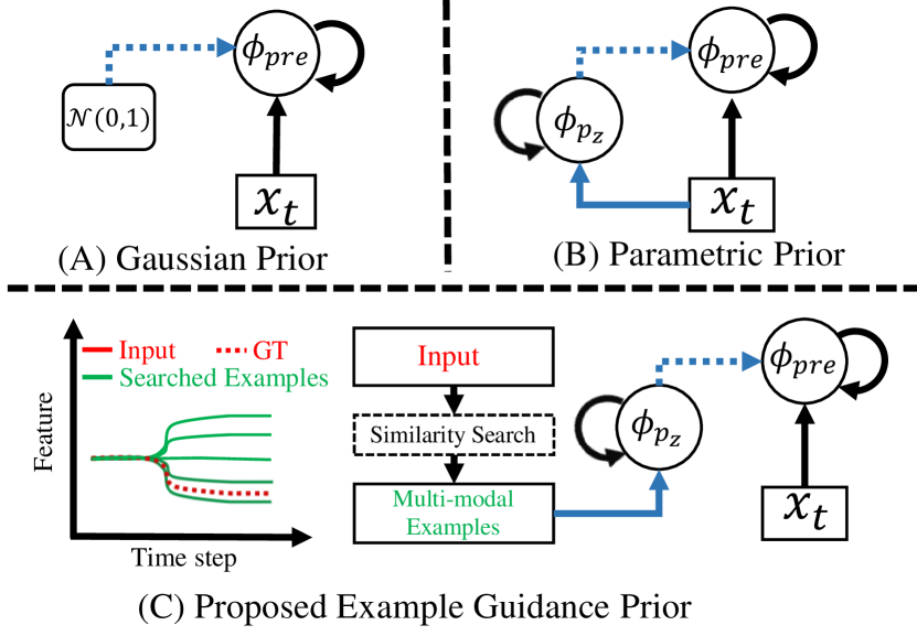
Figure 1: Illustration of stochastic prediction with different prior schemes. Rectangle box refers to input. $\phi_{q_{z}}$ is for uncertainty modelling and $\phi_{pre}$ is the prediction model. We omit the output part for simplicity. Blue line corresponds to stochastic modelling and dashed line is the sampling procedure of random variable. (A) Prediction with fixed Gaussian prior, which does not consider the temporal dependency between different time steps. (B) Prediction with parametric prior, which lacks explicit supervision signal for multi-modal future modelling. (C) Proposed prediction scheme with similar examples retrieved in training dataset. These examples are utilized construct an explicit multi-modal distribution target for the training of prediction model.

Srivastava et al. (2015) first proposes to predict simple digit motion with deep neural models. Video frames are synthesized in a deterministic manner (Denton & Birodkar, 2017), which also suffers to achieve long-range and high-quality prediction, even with large model capacity (Finn et al., 2016). Babaeizadeh et al. (2018) shows that the distribution of frames is a more important aspect that should be modelled. Variational based methods (e.g., SVG (Denton & Fergus, 2018) and SAVP (Lee et al., 2018)) are naturally developed to achieve good performance on simple dynamics such as digit moving (Srivastava et al., 2015) and robot arm manipulation (Finn et al., 2016).

However, real-world motion commonly follows multi-modal distributions. With the increase of motion diversity and complexity, variational inference with prior Gaussian distribution is insufficient to cover the wide spectrum of future possibilities. Meanwhile, downstream tasks mentioned in the first paragraph require prediction model with capability to model real-world distribution (i.e., can the multi-modal motion pattern be effectively captured?) and high sampling efficiency (i.e., fewer samples needed to achieve higher prediction accuracy). These are both important factors for stochastic prediction, which are also the focus issues in this paper. Recent work introduces external information (e.g., object location (Ye et al., 2019; Villegas et al., 2017b)) to ease the prediction procedure, which is hard to generalize to other scenes.

Predictive models can heavily rely on similarity between past experiences and the new ones, implying that sequences with similar motion might fall into the same modal with a high probability. The key insight of our work, deduced from the above observation, is that the potential distribution of sequence to be predicted can be approximated by analogous ones in a data pool, namely, examples.

In other words, our work (termed as VPEG, Video Prediction via Example Guidance) bypasses implicit optimization of latent variable relying on variational inference; as shown in Fig. 1C, we introduce an explicit distribution target constructed from analogous examples, which are empirically proved to be critical for distribution modelling. To guarantee output predictions are multi-modal distributed, we further propose a novel optimization scheme which considers the prediction task as a stochastic process for explicit motion distribution modelling. Meanwhile, we incorporate the adversarial training into proposed method to guarantee the plausibility of each predicted sample. It is also worth mentioning that our model is able to integrate with the majority of existing stochastic predictive models. Implementing our method is simply replacing variational method with the proposed optimization framework. We conduct extensive experiments on several widely used datasets, including moving digit (Srivastava et al., 2015), robot arm motion (Finn et al., 2016), and human activity (Zhang et al., 2013). Considerable enhancement is observed both in quantitative and qualitative aspects. Qualitatively, the high-level semantic structure, e.g., human skeleton topology, could be well preserved during prediction. Quantitatively, our model is able to produce realistic and accurate motion with fewer samples compared to previous methods. Moreover, our model demonstrates generalization ability to predict unseen motion class during testing procedure, which suggests the effectiveness of example guidance.

2 Related Work

Distribution Modelling with Stochastic Process. In this filed, one major direction is based on Gaussian process (denoted as GP)  (Rasmussen & Williams, 2006). Wang et al. (2005) proposes to extend basic GP model with dynamic formation, which demonstrates appealing ability of learning human motion diversity. Another promising branch is determinantal point process (denoted as DPP) (Affandi et al., 2014; Elfeki et al., 2019), which focuses on diversity of modelled distribution by incorporating a penalty term during optimization procedure. Recently, the combination of stochastic process and deep neural network, e.g., neural process (Garnelo et al., 2018) leads to a new routine towards applying stochastic process on large-scale data. Neural process (Garnelo et al., 2018) combines the best of both worlds between stochastic process (data-driven uncertainty modelling) and deep model (end-to-end training with large-scale data). Our work, which treads on a similar path, focuses on the distribution modelling of real-world motion sequences.

Video Prediction. Video prediction is initially considered as a deterministic task which requires a single output at a time (Srivastava et al., 2015). Hence, many works focus on the architecture optimization of the predictive models. Conv-LSTM based model (Shi et al., 2015; Finn et al., 2016; Wang et al., 2017; Xu et al., 2018a; Lotter et al., 2017; Byeon et al., 2018; Wang et al., 2019) is then proposed to enhance the spatial-temporal connection within latent feature space to pursue better visual quality. High fidelity prediction could be achieved by larger model and more computation sources (Villegas et al., 2019). Flow-based prediction model (Kumar et al., 2020) is proposed to increase the interpretability of the predicted results. Disentangled representation learning (Denton & Birodkar, 2017; Gao et al., 2018) is proposed to reduce the difficulty of human motion modelling (Yan et al., 2017) and prediction. Another branch of work (Jia et al., 2016) attempts to predict the motion with dynamic network, where the deep model is flexibly configured according to inputs, i.e., adaptive prediction. Deterministic model is infeasible to handle multiple possibilities. Stochastic video prediction is then proposed to address this problem. SV2P (Babaeizadeh et al., 2018) is firstly proposed as an stochastic prediction framework incorporated with latent variables and variational inference for distribution modelling. Following a similar inspiration, SAVP (Lee et al., 2018) demonstrates that the combination of GAN (Goodfellow et al., 2014) and VAE (Kingma & Welling, 2014) facilitates better modelling of the future possibilities and significantly boosts the generation quality of predicted frames. Denton & Fergus (2018) proposes to model the unknown true distribution in a parametric and learnable manner, i.e., represented by a simple LSTM (Hochreiter & Schmidhuber, 1997) network. Recently, unsupervised keypoint learning (Kim et al., 2019) (i.e., human pose (Xu et al., 2020)) is utilized to ease the modelling difficulty of future frames. Domain knowledge, which helps to reduce the motion ambiguity (Ye et al., 2019; Tang & Salakhutdinov, 2019; Luc et al., 2017), is proved to be effective in future prediction. In contrast to these works above, we are motivated by one insight that prediction is based on similarity between the current situation and the past experiences. More specifically, we argue that the multi-modal distribution could be effectively approximated with analogous ones (i.e., examples) in training data and real-world motion could be further accurately predicted with high sampling efficiency.

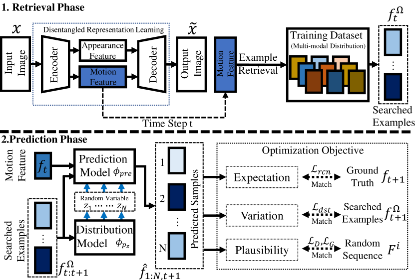
Figure 2: Overall framework of proposed video prediction method. The whole procedure is split into two consecutive phases presented at the top and bottom rows respectively. Top row refers to retrieval process of proposed method, while bottom rows is the prediction model with example guidance. It is optimized as a stochastic process to effectively capture the future motion uncertainty.

3 Method

Given $M$ consecutive frames as inputs, we are to predict the future $N$ frames in the pixel-wise manner. Suppose the input (context) frames $\mathbf{X}$ is of length $M$, i.e., $\mathbf{X}=\{\mathbf{x}_{t}\}_{t=1}^{M}\in\mathbb{R}^{W\times H\times C\times M}$, where $W,H,C$ are image width, height and channel respectively. Following the notation defined, the prediction output $\mathbf{Y}$ is of length $N$, i.e., $\mathbf{Y}=\{\mathbf{y}_{t}\}_{t=1}^{N}\in\mathbb{R}^{W\times H\times C\times N}$. We denote the whole training set as $\mathcal{D}_{s}$. Fig. 2 demonstrates the overall framework of the proposed method. Details are presented in following subsections.

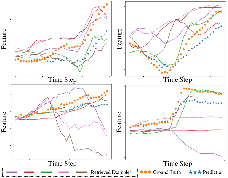
Figure 3: Four typical patterns of retrieved examples on PennAction (Zhang et al., 2013) dataset. The five solid lines refer to top-5 examples searched in $\mathcal{D}_{s}$ and orange-dot line is the ground truth motion sequence. The blue-star line is predicted sequence. The input sequence generally falls into one variation pattern of retrieved examples, which confirms the key insight of our work.

3.1 Example Retrieval via Disentangling Model

We conduct the retrieval procedure in training set $\mathcal{D}_{s}$. To avoid trivial solution, $\mathbf{X}$ is excluded from $\mathcal{D}_{s}$ if $\mathbf{X}$ is in the training set $\mathcal{D}_{s}$. Direct search in the image space is infeasible because it generally contains unnecessary information for retrieval, e.g., the appearance of foreground subject and detailed structure of background. Alternatively, a better solution is retrieving in disentangled latent space. Many previous methods (Denton & Birodkar, 2017; Tulyakov et al., 2018; Villegas et al., 2017a; Denton & Fergus, 2018) have made promising progress in learning to disentangle latent feature. Two competitive methods, i.e., SVG (Denton & Fergus, 2018) and Kim et al. (2019) are adopted as the disentangling model in our work.  Kim et al. (2019) proposes an unsupervised method to extract keypoints of arbitrary object, whose pretrained model is directly used to extract the pose information as motion feature in our work. Note that the motion feature remains valid when input is only one frame, where the single state is treated as motion feature. SVG (Denton & Fergus, 2018) unifies the disentangling model and variational inference based prediction into one stage. We remove the prediction part and train the disentangling model as:

$$(\mathbf{b}_{t},\mathbf{h}_{t}) =\phi_{dse}(\mathbf{x}_{t}),t\in\{i,j\},$$ (1)

$$\mathcal{L}_{dse} =||\phi_{dec}(\mathbf{b}_{i},\mathbf{h}_{j})-\mathbf{x}_{j}||_{2}^{2},$$ (2)

where $i,j$ are two random time steps sampled from one sequence, $\phi_{dse}$ and $\phi_{dec}$ are disentangling model and decoder (for image reconstruction) respectively. $\mathcal{L}_{dse}$ indicates two frames from the same sequence share similar background and should be able to reconstruct each other by exchanging the motion feature. By optimizing this loss function, appearance feature $\mathbf{b}_{*}$ is expected to be constant while $\mathbf{h}_{*}$ contains the motion information, which leads the disentanglement model to learn to extract motion feature in a self-supervised way. Both disentanglement models SVG (Denton & Fergus, 2018) and Kim et al. (2019) could be presented in a unified way as shown in Fig. 2. Next we focus on the retrieval procedure. Note that all input frames are used in this part. We denote the feature used for retrieval as $\mathbf{F}\in\mathbb{R}^{C_{f}\times M}=\{\mathbf{f}_{t}\}_{t=1}^{M}$, where $C_{f}$ is the number of feature dimension.

Given input sequence $\mathbf{X}$, whose motion feature denoted as $\mathbf{F}$, and training set $\mathcal{D}_{s}$, we conduct nearest-neighbor search as:

$$\Omega_{i}=\mathcal{S}(||\mathbf{F}^{i}-\mathbf{F}||_{2}^{2},K),$$ (3)

where $\mathbf{F}^{i}$ refers to the extracted feature of $\mathbf{X}^{i}\in\mathcal{D}_{s}$. $\mathcal{S}(\bullet,K)$ refers to top $K$ selection from a set in the ascending order. $\Omega_{i}$ is the retrieved index set corresponding to $i$th sample. Note that the subscript $i$ is omitted for simplicity in following contexts. $K$ is treated as a hyper-parameter in our experiments, whose influence is validated through ablation study in Sec. 4. We perform first-order difference along the temporal axis to focus on state difference during the retrieval procedure if multiple frames are available. We plot retrieved examples (solid line, $K=5$) together with the input sequence (orange-dot line) in Fig. 3. Here we have two main observations: (1) The input sequence generally falls into one motion pattern of retrieved examples, which confirms the key insight of our work. (2) The examples have non-Gaussian distribution, which implies the difficulty on the optimization side by a variational inference method. We present more visual evidence in supplementary material to demonstrate the common existence of such similarity between $\mathbf{F}$ and $\mathbf{F}^{\Omega}$.

Discussion of Retrieval Efficiency. Note that the retrieval module is introduced in this work, which is an additional step compared to the majority of previous methods. One concern would thus be the retrieval time, which is highly correlated with efficiency of the whole model. We would like to clarify that the retrieval step is highly efficient: (1) It is executed in the low dimensional feature space (i.e., $\mathbf{f}\in\mathbb{R}^{C_{f}}$) rather than in the image space, which requires less computation; (2) It is implemented with the efficient quick-sort algorithm. The averaged retrieval complexity is O(NlogN), where N is the number of video sequences. For example, on the PennAction dataset (Zhang et al., 2013) (containing 1172 sequences in total) the whole running (including retrieval) time of predicting 32 frames is 354ms, while the retrieval time only takes 80ms.

3.2 Example Guided Multi-modal Prediction

3.2.1 Stochastic Video Prediction Revisited

The majority works (Denton & Birodkar, 2017; Ye et al., 2019; Denton & Fergus, 2018; Lee et al., 2018) of stochastic video prediction are based on variational inference. We first briefly review previous works in this field and then analyze the inferiority of stochastic prediction based on variational inference.

These methods use a latent variable (denoted as $\mathbf{z}$) to model the future uncertainty. The distribution of $\mathbf{z}$ (denoted as $p_{z}$) is trained to match with a (possibly fixed) prior distribution (denoted as $q_{z}$) as follows,

$$\mathcal{L}=||\phi_{pre}(\mathbf{F}_{1:t-1},\mathbf{z}_{t})-\mathbf{f}_{t}||_{2}^{2}+\mathcal{L}_{KL}(p_{z}||q_{z}),$$ (4)

where $\phi_{pre}$, $q_{z}$, $\mathcal{L}_{KL}()$ are the prediction model, target distribution and Kullback-Leibler divergence function (Kullback & Leibler, 1951) respectively. $p_{z}$ is generally modelled with deep neural network (e.g., $\phi_{p_{z}}(\mathbf{f}_{t-1})$). $q_{z}$ is fixed, e.g., $\mathcal{N}(\mathbf{0},\mathbf{I})$. This implies that the predicted image $\mathbf{X}_{t}$ is controlled by $\mathcal{N}(\mathbf{0},\mathbf{I})$, not real-world motion distribution. Denton & Fergus (2018) proposes to model the potential distribution with $\phi_{q_{z}}(\mathbf{f}^{t})$, which still lacks an explicit supervision signal on the distribution of motion feature.

The essence of the modelling difficulty is from the optimization target of the $\mathcal{L}_{KL}$ term. Under the framework of variational inference, the form of $q_{z}$ is generally restricted to a normal distribution for tractability. However, this is in conflict with the multi-modal distribution nature of real-world motion. We need a more explicit and reliable target and thus propose to construct it with similar examples $\mathbf{f}^{\Omega}$ whose retrieval procedure is described in Sec. 3.1.

Algorithm 1 Example Guided Video Prediction

  Input: Training Set $\mathcal{D}_{s}$, disentangling model $\phi_{dse}$, predictor $\phi_{pre}$ and discriminator $\phi_{dcm}$. $\#$Example retrieval phase

  for Input sequence $\mathbf{X}$ in $\mathcal{D}_{s}$ do

     Get motion feature $\mathbf{F}=\phi_{dse}(\mathbf{X})$,

     Example retrieval to obtain $\mathbf{F}^{\Omega}$ as Eqn. 3.

  end for$\#$Prediction phase

  repeat

     Get a random batch of $(\mathbf{F},\mathbf{F}^{\Omega})$ pairs. $\#$Optimization as a stochastic process

     for $i=1$ to $N$ do

        Sample noise $\mathbf{z}_{i,t+1}$ as Eqn. 8,

        Predict next state $\hat{\mathbf{f}}_{i,t+1}$ as Eqn. 9,

     end for

     Optimize w.r.t. Eqn. 10, 11, 12 and 13.

  until the training objective $\mathcal{L}_{fin}$ (Eqn. 14) converged.

3.2.2 Prediction with Examples

Given retrieved examples $\mathbf{f}^{\Omega}$, we first construct a new distribution target and then learn to approximate it. The most straightforward way is directly replacing the prior distribution $q_{z}$ with the new one. More specifically, at time step $t$ the distribution model $\phi_{p_{z}}$ is trained as:

$$\hat{\mu}_{t},\hat{\sigma}_{t}=\phi_{p_{z}}(\hat{\mathbf{F}}_{1:t-1}),\mathbf{z}_{t}\sim\mathcal{N}(\hat{\mu}_{t},\hat{\sigma}_{t}),$$ (5)

$$\mu_{t},\sigma_{t}=\phi_{q_{z}}(\mathbf{f}^{\Omega}_{t}),\mathcal{L}_{KL}=\log(\frac{\sigma_{t}}{\hat{\sigma}_{t}})+\frac{\hat{\sigma}_{t}+(\mu_{t}-\hat{\mu}_{t})^{2}}{2\sigma_{t}},$$ (6)

where $\mathbf{z}_{t}$ models the possibility of future state and $\mu_{t},\sigma_{t}$ are commonly supervised with $\mathcal{L}_{KL}$.

However, it is difficult to obtain promising results with the above method which simply replaces $\mathbf{f}_{t}$ with $\mathbf{f}^{\Omega}_{t}$. The reason mainly lies in two aspects: Firstly, the diversity of predicted motion feature at time step $t$ (denoted as $\hat{\mathbf{f}}_{t}$) lacks an explicit supervision signal. Secondly, the distribution of latent variable $\mathbf{z}_{t}$ (i.e., $\mathcal{N}(\mu_{t},\sigma_{t})$) is infeasible to accurately represent the motion diversity of $\mathbf{f}_{t}^{\Omega}$, because no dedicated training objective is designed for this target.

Optimization as Stochastic Process. Motivated by the above two issues, we consider the prediction task as a stochastic process targeting at explicit distribution modelling. The whole prediction procedure is conducted in motion feature space. The inputs of prediction model $\phi_{pre}$ include $\mathbf{f}^{\Omega}_{t}$ and $\mathbf{f}_{t}$. We calculate the mean and variance of example feature $\mathbf{f}^{\Omega}_{t}$, i.e., $\mathcal{E}(\mathbf{f}^{\Omega}_{t})$ and $\mathcal{V}(\mathbf{f}_{t})$, for the subsequent random sampling in motion space. The prediction procedure at time step $t$ is conducted as follows,

$$(\mu_{t},\sigma_{t})=\phi_{q_{z}}(\mathcal{E}(\mathbf{f}_{t}^{\Omega}),\mathcal{V}(\mathbf{f}_{t}^{\Omega})),$$ (7)

$$(\mathbf{z}_{1,t},...,\mathbf{z}_{N,t})\stackrel{{\scriptstyle\mathrm{i.i.d.}}}{{\sim}}\mathcal{N}(\mu_{t},\sigma_{t}),$$ (8)

$$\hat{\mathbf{f}}_{i,t+1}=\phi_{pre}(\hat{\mathbf{f}}_{i,t},\mathbf{z}_{i,t},\mathbf{f}_{t}^{\Omega}),i=1,...,N,$$ (9)

where $(\mathbf{z}_{1,t},...,\mathbf{z}_{N,t})$ is a group of independent and identically sampled values and $\mathbf{z}_{i,t}\in\mathbb{R}^{h}$. The subscript ${i,t}$ refers to $i$th sample at time step $t$. Predicted state $\hat{\mathbf{f}}_{i,t}$ is not fed into $\phi_{q_{z}}$, where we empirically get sub-optimal results. Because at initial training stage $\hat{\mathbf{f}}_{i,t}$ is noisy and non-informative, which in turn acts as a distractor for training $\phi_{q_{z}}$. The prediction model is trained as follows,

$$\mathcal{L}_{rcn}=||\hat{\mathbf{f}}_{j,t+1}-\mathbf{f}_{t+1}||_{2}^{2},$$ (10)

$$\mathcal{L}_{dst}=||\mathcal{V}(\{\hat{\mathbf{f}}_{i,t+1}\}_{i=1}^{N})-\mathcal{V}(\mathbf{f}_{t+1}^{\Omega})||_{2}^{2},$$ (11)

where $j=\min_{i}||\{\hat{\mathbf{f}}_{i,t+1}\}_{i=1}^{N}-\mathbf{f}_{t+1}||_{2}^{2}$. $\mathcal{L}_{rcn}$ indicates that the best matched one is used for training (Xu et al., 2018b). Empirically, it is proved to be useful for stabilizing prediction when having multiple outputs.

$\mathcal{L}_{dst}$ aims to restrict the variety of $N$ predicted features to match with $\mathbf{f}_{t+1}^{\Omega}$. In this way, the motion information of examples is effectively utilized and the distribution of predicted sequences is explicitly supervised. Meanwhile, to guarantee the plausibility of each predicted sequence, we incorporate the adversarial training into our method. More specifically, a motion discriminator $\phi_{dcm}$ is utilized to facilitate realistic prediction.

$$\mathcal{L}_{D}=\frac{1}{2}(\phi_{dcm}(1-\mathbf{F})+\phi_{dcm}(1+\hat{\mathbf{F}}_{i})),$$ (12)

$$\mathcal{L}_{G}=-\phi_{dcm}(1-\hat{\mathbf{F}}_{i}),$$ (13)

where $i\in[1,N]$, $\mathcal{L}_{D},\mathcal{L}_{G}$ are adversarial losses for $\phi_{dcm}$ and $\phi_{pre}$ (Goodfellow et al., 2014). Adversarial training effectively guarantees the predicted sequence not drifting far away from the real-wold motion examples. For clarity we present the whole prediction procedure in Alg. 1.

Improvement upon existing models. Our work mainly focuses on multi-modal distribution modelling and sampling efficiency, which is adaptive to multiple neural models. In Sec. 4, we demonstrate extensive results by combining proposed framework with two baselines, i.e., SVG (Denton & Fergus, 2018) and Kim et al. (2019). The final objective is shown below:

$$\mathcal{L}_{fin}=\lambda_{1}\mathcal{L}_{rcn}+\lambda_{2}\mathcal{L}_{dst}+\lambda_{3}\mathcal{L}_{D}+\lambda_{4}\mathcal{L}_{G}.$$ (14)

For training and implementation details, (hyper-parameter and network architecture), please refer to the supplementary material.

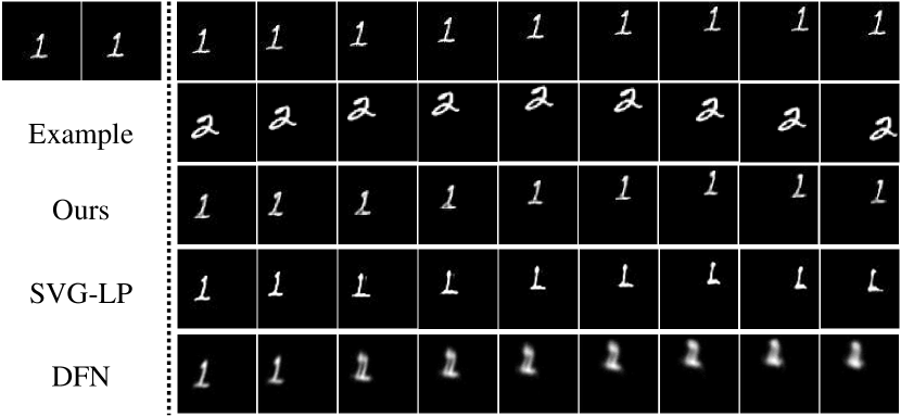
Figure 4: Visualization of prediction results on MovingMnist (Srivastava et al., 2015) dataset under stochastic setting. First row refers to ground truth. Following three rows correspond to example, predicted sequences of proposed model, SVG (Wichers et al., 2018) and DFN (Shi et al., 2015) respectively.

4 Experiments

4.1 Datasets and Evaluation Metrics

We evaluate our model with three widely used video prediction datasets: (1) MovingMnist (Srivastava et al., 2015), (2) Bair RobotPush (Ebert et al., 2017) and (3) PennAction (Zhang et al., 2013). Following the evaluation practice of SVG (Babaeizadeh et al., 2018) and Kim et al. (2019), we calculate the per-step prediction accuracy in terms of PSNR and SSIM. The overall prediction quality of video frames is evaluated with Fréchet Video Distance (FVD) (Unterthiner et al., 2018). To ensure fair evaluation, we compare with models whose source code is publicly available. Specifically, on MovingMnist (Srivastava et al., 2015) dataset we compare with SVG (Denton & Fergus, 2018) and DFN (Shi et al., 2015); On RobotPush (Ebert et al., 2017) dataset SVG (Denton & Fergus, 2018), SV2P (Babaeizadeh et al., 2018) and CDNA (Finn et al., 2016) are treated as baselines; On PennAction (Zhang et al., 2013) dataset the works of Kim et al. (2019); Li et al. (2018); Wichers et al. (2018); Villegas et al. (2017b) are used for comparison. Note that to follow the best practice of the baseline model (Kim et al., 2019), the prediction procedure on the PennAction Dataset (Zhang et al., 2013) is a implementation-wise variant of Eqn. 7-9. More specifically, the random noise is sampled only at the first time stamp. Please refer to prediction procedure of the baseline model (Kim et al., 2019) for more details. In all experiments we empirically set $N=K=5$.

Mode	Model	T=1	T=3	T=5	T=7	T=9	T=11	T=13	T=15	T=17
D	DFN	25.3	23.8	22.9	22.0	21.2	20.1	19.5	19.1	18.9
	SVG-LP	24.7	22.8	21.3	19.5	18.8	18.2	17.9	17.7	17.4
	Ours	25.6	23.2	22.5	21.7	20.8	20.3	19.8	19.5	19.3
S	DFN	25.1	22.1	18.9	16.5	16.2	15.7	15.2	14.9	14.3
	SVG-LP	25.4	23.9	22.9	19.5	19.0	18.7	18.7	18.2	17.6
	Ours	26.0	24.8	23.1	22.1	21.0	20.5	19.7	19.5	19.2

Table 1: Prediction accuracy on MovinMnist dataset (Srivastava et al., 2015) in terms of PSNR. Mode refers to experiment setting, i.e., stochastic (S) or deterministic (D). We compare our model with SVG-LP (Denton & Fergus, 2018) and DFN (Jia et al., 2016).

4.2 Motivating Experiments: Moving Digit Prediction

For MovingMnist (Srivastava et al., 2015) dataset, inputs/outputs are of length 5 and 10 respectively during training. Note that this dataset is configured with two different settings, i.e., to be deterministic or stochastic. The deterministic version implies that the motion is determined by initial direction and velocity, while for the stochastic one, a new direction and velocity are applied after the digit hitting the boundary. The prediction model should be able to accurately estimate motion patterns under both settings.

Deterministic Motion Prediction. Tab. 1 shows prediction accuracy (in terms of PSNR) from T=1 to T=17. One can observe that our model outperforms SVG-LP (Denton & Fergus, 2018) by a large margin and is comparable to DFN (Jia et al., 2016). Under deterministic setting the retrieved examples provide exact motion information to facilitate prediction procedure. We present corresponding visual results in supplementary material and please refer to it.

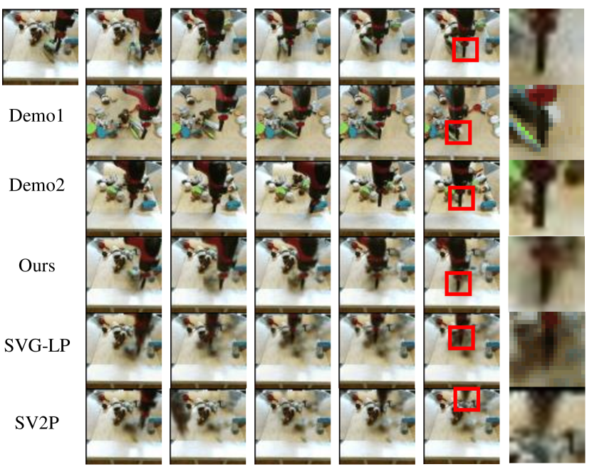
Figure 5: Comparison of the predicted sequences on RobotPush (Ebert et al., 2017) dataset. Rows from top to bottom: ground truth, two retrieved examples, predicted results of our model, SVG (Denton & Fergus, 2018) and SV2P (Babaeizadeh et al., 2018).

Stochastic Motion Prediction. Under stochastic setting, the best PSNR value of 20 random samples is reported (bottom three rows of Tab. 1). Considerable improvement over SVG-LP (Denton & Fergus, 2018) could be observed from Tab. 1. Despite the retrieved example sequence not perfectly matching with ground truth (Fig. 4, first two columns refer to input.), informative motion pattern is provided, i.e., bouncing back after reaching the boundary. The deterministic model (DFN (Jia et al., 2016)), which only produces a single output, is infeasible to properly handle stochastic motion. For example, the blur effect (last row in Fig. 4) is observed after hitting the boundary.

Deterministic and stochastic datasets possess different motion patterns and distributions. Non-stochastic method (e.g., DFN (Jia et al., 2016)) is insufficient to capture motion uncertainty, while SVG-LP (Denton & Fergus, 2018), empirically restricted by the stochastic prior nature in variational inference, is not capable of accurately predicting the trajectory under the deterministic condition. Under deterministic setting, retrieved examples generally follow similar trajectory, whose variance is low. For the stochastic version, searched sequences are highly diverse but follow the same motion pattern, i.e., bouncing back when hitting the boundary. Guided by examples from these experiences, our model is able to reliably capture the motion pattern under both settings. It implies that compared to fixed/learned prior, the motion variety could be better represented by similar examples. Please refer to supplementary material for more visual results.

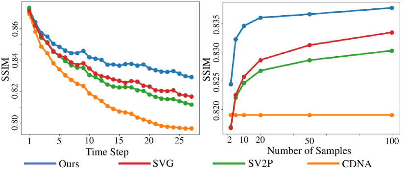
Figure 6: Evaluation in terms of SSIM on RobotPush (Ebert et al., 2017) dataset. Left figure: X-axis is the time step and Y-axis is SSIM. Right figure: X-axis refers to the number of random samples during evaluation and Y-axis is averaged SSIM over a whole predicted sequence.

4.3 Robot Arm Motion Prediction

Experiments on RobotPush (Ebert et al., 2017) dataset take 5 frames as inputs and predict the following 10 frames during training. As illustrated in Fig. 6 (first column refers to input), we present quantitative evaluation in terms of SSIM. For the stochastic method, the best value of 20 random samples is presented. Fig. 6 implies that our method outperforms all previous methods by a large margin. We find CDNA (Finn et al., 2016) (deterministic method) is inferior to stochastic ones. We attribute this to the high uncertainty of robot motion in this dataset. Our model, facilitated by example guidance, is capable of capturing the real motion dynamics in a more efficient manner. To comprehensively evaluate the distribution modelling ability and sampling efficiency of the proposed method, we calculate the mean accuracy w.r.t. the number of samples (denoted as $P$): Fig. 6 shows the accuracy improvement for all stochastic methods along with the increase of $P$, which tends to be saturated when $P$ is large. It is worth mentioning that our model still outperforms SVG (Denton & Fergus, 2018) by a large margin when $P$ is sufficiently large, e.g., 100. This clearly indicates a higher upper bound of accuracy achieved by our model (with guidance of retrieved examples) compared to variational inference based method, i.e., superior capability to capture real-world motion pattern.

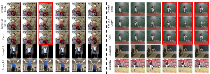
Figure 7: Qualitative evaluation of human motion prediction on PennAction (Zhang et al., 2013) dataset. We present ground truth, results of Kim et al. (2019), predicted sequence of our model and two searched examples. The left part refers to a pull-up action with multi-modal futures based on the current input and searched examples are capable of matching with possibilities. The right part aims to show that our model is capable of preserving the general structure during prediction. Red-boxes highlight the corresponding evidences on both sides.

Metric	[1]	[2]	[3]	[4]	Ours
Action Acc$\uparrow$	15.89	40.00	47.14	68.89	73.23
FVD$\downarrow$	4083.3	3324,9	2187.5	1509.0	1283.5

Table 2: Quantitative evaluation of predicted sequences in terms of Fréchet Video Distance (FVD) (Unterthiner et al., 2018) (lower is better) and action recognition accuracy (higher is better). Previous works [1]-[4] refer to (Li et al., 2018; Wichers et al., 2018; Villegas et al., 2017b) respectively. Experiment is conducted on PennAction dataset (Zhang et al., 2013).

Predicted sequences are shown in Fig. 5. For row arrangement please refer to the caption. The key region (highlighted with red boxes) of predicted frames is zoomed in for better visualization of details (last column). Compared to stochastic baselines, our model achieves higher image quality of predicted sequences, i.e., object edges and general structure are better preserved. Meanwhile, the overall trajectory is more accurately predicted by our model if compared to two stochastic baselines, which is mainly facilitated by the effective guidance of retrieved examples. For more visual results please refer to the supplementary material.

Metric	K=2	K=3	K=4	K=5	K=6	K=7
PSNR	17.81	18.19	18.28	18.35	18.31	18.25
SSIM	0.78	0.82	0.83	0.84	0.84	0.83

Table 3: Influence of the example number $K$ evaluated in terms of PSNR (first row) and SSIM (second row) on RobotPush (Ebert et al., 2017) dataset. Note that each number reported in this table is averaged over the whole predicted sequence.

4.4 Human Motion Prediction

We report the experimental results on a human daily activity dataset, i.e., PennAction (Zhang et al., 2013). We follow the setting of Kim et al. (2019), which is also a strong baseline for comparison. More specifically, the class label and first frame are fed as inputs. Note that under this situation we retrieve the examples according to the first frame in sequences with an identical action label.

To evaluate the multi-modal distribution modelling capability, Fig. 7A presents the best prediction sequence of 20 random samples in terms of PSNR and please refer to the caption for row arrangement. First column refers to input. The pull-up action generally possesses two motion modalities, i.e., up and down. We can observe that Kim et al. (2019) fails to predict corresponding motion precisely even with 20 samples (third time step highlighted with red-boxes). Our model, guided by similar examples (last two rows in Fig. 7A), is capable of synthesizing the correct motion pattern compared to the groundtruth sequence. Meanwhile, from Fig. 7B we can notice that Kim et al. (2019) fails to preserve the general structure during prediction. The human topology is severely distorted especially at the late stage of prediction (last 3 time steps highlighted with red-boxes). As comparison the structure of subject is well maintained predicted by our model, which is visually more natural than the results of Kim et al. (2019). This implies reliably capturing the motion distribution facilitates better visual quality of final predicted image sequences. We present more visual results in supplementary material and please refer to it.

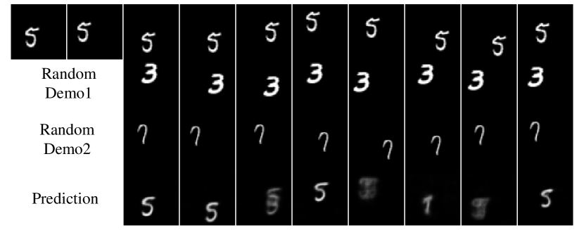
Figure 8: Prediction results with random example guidance on MovingMnist (Srivastava et al., 2015) dataset. The top and bottom rows correspond to ground truth and predicted sequence, while the middle two rows are randomly selected examples in this dataset. Unnatural motion is observed during prediction (last row).

For quantitative evaluation, we follow Kim et al. (2019) to calculate the action recognition accuracy and FVD (Unterthiner et al., 2018) score. As shown in Tab. 2, our model outperforms all previous methods in terms of both action recognition accuracy and FVD score by a large margin. This mainly benefits from the retrieved examples, which provides effective guidance for future prediction.

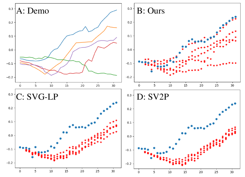
Figure 9: Visualization of retrieved examples and randomly sampled sequences on RobotPush (Ebert et al., 2017) dataset. Top left refers to searched examples, while the other three figures correspond to sampled sequences by proposed model, SVG (Wichers et al., 2018) and SV2P (Babaeizadeh et al., 2018) respectively.

4.5 Ablation Study

Does example guidance really help? To evaluate the effectiveness of retrieved examples, we replace the retrieval procedure described in Sec. 3.1 with the random selection, i.e., the examples have no motion similarity with inputs. We conduct this experiment on MovingMnist (Srivastava et al., 2015) dataset. Results are presented in Fig. 8 and please refer to caption for detailed row arrangement. Due to the lack of motion similarity between examples and the input sequence, the predicted sequence demonstrates unnatural motion. The double-image effect of digit 5 (last row in Fig. 8), resulting from the misleading information of motion trajectory provided by random examples, implies the critical value of retrieval procedure proposed in Sec. 3.1. In supplementary material, we also present visualization evidence to demonstrate the inferiority of simply combining example guidance and variational inference. Please refer to it.

Does the proposed model really capture multi-modal distribution? We present the sampled motion features (Fig. 9) in RobotPush (Ebert et al., 2017) dataset to evaluate the capability of distribution modelling. For row arrangement please refer to the caption. For sub-figures from B to D, red-dot lines refer to predicted sequences and blue ones are ground truth. We can observe that the sampled states of SVG (Denton & Fergus, 2018) and SV2P (Babaeizadeh et al., 2018) are not multi-modal distributed. Guided by retrieved examples whose multi-modality distribution generally cover the ground truth motion, our model is able to predict the future motion in a more efficient way. Meanwhile, we present more visualization results to show that predicted sequences are not simply copied from examples and they are highly diverse.

Influence of Example Number $K$. As illustrated in Tab. 3, we conduct corresponding ablation study about $K$ on RobotPush (Ebert et al., 2017) dataset. Performance under two metrics, i.e., PSNR and SSIM, is reported. PSNR and SSIM are averaged over the whole sequence and the best of 20 random sequences is reported. $K$ ranges from 2 to 7. We can see that both PSNR and SSIM keep increase when $K$ is no larger than 5 and then decrease. It indicates that multi-modal examples facilitate better modelling the target distribution, but noise information (or irrelevant motion pattern) might be introduced when $K$ is too large.

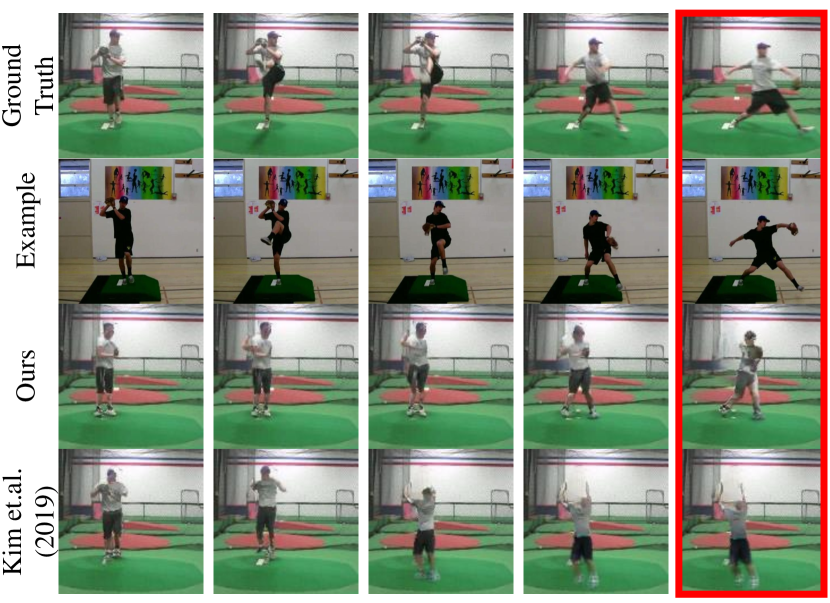
Figure 10: Predicted results of unseen motion. Contents from top to bottom are ground truth sequence, retrieved example, prediction of our model and the results of (Kim et al., 2019) respectively.

4.6 Motion Prediction Beyond Seen Class

To further evaluate the generalization ability of the proposed model, we are motivated to predict the motion sequence on unseen class. The majority of video prediction methods are merely able to forecast the motion pattern accessible during training, which are hardly generalizable to novel motion. We conduct experiments on PennAction (Zhang et al., 2013) dataset. We choose three actions, i.e., golf_swing, pull_ups and tennis_serve as known action during training and baseball_pitch as the unseen motion used during testing. Our model as well as that of Kim et al. (2019) is retrained without label class. During testing, the examples for guidance are retrieved baseball_pitch sequences. Fig. 10 demonstrates the predicted results. For row arrangement please refer to the caption. We can observe that Kim et al. (2019) fails to give rational prediction regarding the input, where there should be a baseball_pitch motion but visually resemble tennis_serve. Facilitated by the guidance of examples, our model produces a visually natural tennis_serve sequence, which clearly demonstrates the generalization capability of proposed model. We argue that the majority of previous works are (implicitly) forced to memorize motion categories in the training set. In contrast to the paradigm, our work is relieved from such burden because the retrieved examples contain the category information in assistance of prediction. We thus focus only on intra-class diversity. If given examples with unseen motion categories, our model is still able to give reasonable predictions, thanks to the example guidance. We present more visual results in supplementary material and please refer to it.

5 Conclusion

In this work, we present a simple yet effective framework for multi-modal video prediction, which mainly focuses on the capability of multi-modal distribution modelling. We first retrieve similar examples in the training set and then use these searched sequences to explicitly construct a distribution target. With proposed optimization method based on stochastic process, our model achieves promising performance on both prediction accuracy and visual quality.

References

- Affandi et al. (2014) Affandi, R. H., Fox, E. B., Adams, R. P., and Taskar, B. Learning the parameters of determinantal point process kernels. In ICML, 2014.
- Babaeizadeh et al. (2018) Babaeizadeh, M., Finn, C., Erhan, D., Campbell, R. H., and Levine, S. Stochastic variational video prediction. In ICLR, 2018.
- Byeon et al. (2018) Byeon, W., Wang, Q., Srivastava, R. K., and Koumoutsakos, P. Contextvp: Fully context-aware video prediction. In ECCV, 2018.
- Denton & Fergus (2018) Denton, E. and Fergus, R. Stochastic video generation with a learned prior. In ICML, 2018.
- Denton & Birodkar (2017) Denton, E. L. and Birodkar, V. Unsupervised learning of disentangled representations from video. In NeurIPS, 2017.
- Ebert et al. (2017) Ebert, F., Finn, C., Lee, A. X., and Levine, S. Self-supervised visual planning with temporal skip connections. In CoRL, 2017.
- Elfeki et al. (2019) Elfeki, M., Couprie, C., Rivière, M., and Elhoseiny, M. GDPP: learning diverse generations using determinantal point processes. In ICML, 2019.
- Finn et al. (2016) Finn, C., Goodfellow, I. J., and Levine, S. Unsupervised learning for physical interaction through video prediction. In NeurIPS, 2016.
- Gao et al. (2018) Gao, H., Xu, H., Cai, Q., Wang, R., Yu, F., and Darrell, T. Disentangling propagation and generation for video prediction. CoRR, 2018.
- Garnelo et al. (2018) Garnelo, M., Rosenbaum, D., Maddison, C., Ramalho, T., Saxton, D., Shanahan, M., Teh, Y. W., Rezende, D. J., and Eslami, S. M. A. Conditional neural processes. In ICML, 2018.
- Goodfellow et al. (2014) Goodfellow, I. J., Pouget-Abadie, J., Mirza, M., Xu, B., Warde-Farley, D., Ozair, S., Courville, A. C., and Bengio, Y. Generative adversarial nets. In NeurIPS, 2014.
- Hochreiter & Schmidhuber (1997) Hochreiter, S. and Schmidhuber, J. Long short-term memory. Neural Computation, 1997.
- Jia et al. (2016) Jia, X., Brabandere, B. D., Tuytelaars, T., and Gool, L. V. Dynamic filter networks. In NIPS, 2016.
- Kim et al. (2019) Kim, Y., Nam, S., Cho, I., and Kim, S. J. Unsupervised keypoint learning for guiding class-conditional video prediction. In NeurIPS, 2019.
- Kingma & Welling (2014) Kingma, D. P. and Welling, M. Auto-encoding variational bayes. In ICLR, 2014.
- Kullback & Leibler (1951) Kullback, S. and Leibler, R. A. Ann. Math. Statist., 1951.
- Kumar et al. (2020) Kumar, M., Babaeizadeh, M., Erhan, D., Finn, C., Levine, S., Dinh, L., and Kingma, D. Videoflow: A conditional flow-based model for stochastic video generation. In ICLR, 2020.
- Kurutach et al. (2018) Kurutach, T., Tamar, A., Yang, G., Russell, S. J., and Abbeel, P. Learning plannable representations with causal infogan. In NeurIPS, 2018.
- Lee et al. (2018) Lee, A. X., Zhang, R., Ebert, F., Abbeel, P., Finn, C., and Levine, S. Stochastic adversarial video prediction. CoRR, 2018.
- Li et al. (2018) Li, Y., Fang, C., Yang, J., Wang, Z., Lu, X., and Yang, M. Flow-grounded spatial-temporal video prediction from still images. In ECCV, 2018.
- Lotter et al. (2017) Lotter, W., Kreiman, G., and Cox, D. D. Deep predictive coding networks for video prediction and unsupervised learning. In ICLR, 2017.
- Luc et al. (2017) Luc, P., Neverova, N., Couprie, C., Verbeek, J., and LeCun, Y. Predicting deeper into the future of semantic segmentation. In ICCV, 2017.
- Nair et al. (2018) Nair, A., Pong, V., Dalal, M., Bahl, S., Lin, S., and Levine, S. Visual reinforcement learning with imagined goals. In NeurIPS, 2018.
- Pathak et al. (2017) Pathak, D., Agrawal, P., Efros, A. A., and Darrell, T. Curiosity-driven exploration by self-supervised prediction. In ICML, 2017.
- Rasmussen & Williams (2006) Rasmussen, C. E. and Williams, C. K. I. Gaussian processes for machine learning. 2006.
- Shi et al. (2015) Shi, X., Chen, Z., Wang, H., Yeung, D., Wong, W., and Woo, W. Convolutional LSTM network: A machine learning approach for precipitation nowcasting. In NeurIPS, 2015.
- Srivastava et al. (2015) Srivastava, N., Mansimov, E., and Salakhutdinov, R. Unsupervised learning of video representations using lstms. In ICML, 2015.
- Tang & Salakhutdinov (2019) Tang, Y. C. and Salakhutdinov, R. Multiple futures prediction. In NIPS, 2019.
- Tulyakov et al. (2018) Tulyakov, S., Liu, M., Yang, X., and Kautz, J. Mocogan: Decomposing motion and content for video generation. In CVPR, 2018.
- Unterthiner et al. (2018) Unterthiner, T., van Steenkiste, S., Kurach, K., Marinier, R., Michalski, M., and Gelly, S. Towards accurate generative models of video: A new metric & challenges. CoRR, 2018.
- Villegas et al. (2017a) Villegas, R., Yang, J., Hong, S., Lin, X., and Lee, H. Decomposing motion and content for natural video sequence prediction. In ICLR, 2017a.
- Villegas et al. (2017b) Villegas, R., Yang, J., Zou, Y., Sohn, S., Lin, X., and Lee, H. Learning to generate long-term future via hierarchical prediction. In ICML, 2017b.
- Villegas et al. (2019) Villegas, R., Pathak, A., Kannan, H., Erhan, D., Le, Q. V., and Lee, H. High fidelity video prediction with large stochastic recurrent neural networks. In Wallach, H. M., Larochelle, H., Beygelzimer, A., d’Alché-Buc, F., Fox, E. B., and Garnett, R. (eds.), NeurIPS, 2019.
- Wang et al. (2005) Wang, J. M., Fleet, D. J., and Hertzmann, A. Gaussian process dynamical models. In NeurIPS, 2005.
- Wang et al. (2017) Wang, Y., Long, M., Wang, J., Gao, Z., and Yu, P. S. Predrnn: Recurrent neural networks for predictive learning using spatiotemporal lstms. In NIPS, 2017.
- Wang et al. (2019) Wang, Y., Jiang, L., Yang, M., Li, L., Long, M., and Fei-Fei, L. Eidetic 3d LSTM: A model for video prediction and beyond. In ICLR, 2019.
- Wichers et al. (2018) Wichers, N., Villegas, R., Erhan, D., and Lee, H. Hierarchical long-term video prediction without supervision. In ICML, 2018.
- Xu et al. (2018a) Xu, J., Ni, B., Li, Z., Cheng, S., and Yang, X. Structure preserving video prediction. In CVPR, 2018a.
- Xu et al. (2018b) Xu, J., Ni, B., and Yang, X. Video prediction via selective sampling. In NeurIPS, 2018b.
- Xu et al. (2020) Xu, J., Yu, Z., Ni, B., Yang, J., Yang, X., and Zhang, W. Deep kinematics analysis for monocular 3d human pose estimation. In CVPR, 2020.
- Yan et al. (2017) Yan, Y., Xu, J., Ni, B., Zhang, W., and Yang, X. Skeleton-aided articulated motion generation. In ACM MM, 2017.
- Ye et al. (2019) Ye, Y., Singh, M., Gupta, A., and Tulsiani, S. Compositional video prediction. In ICCV, 2019.
- Zhang et al. (2013) Zhang, W., Zhu, M., and Derpanis, K. G. From actemes to action: A strongly-supervised representation for detailed action understanding. In ICCV, 2013.