${\overline{\rm MS}}$ renormalization of $S$-wave quarkonium wavefunctions at the origin

Abstract

We compute $S$-wave quarkonium wavefunctions at the origin in the $\overline{\rm MS}$ scheme based on nonrelativistic effective field theories. We include the effects of nonperturbative long-distance behaviors of the potentials, while we determine the short-distance behaviors of the potentials in perturbative QCD. We obtain $\overline{\rm MS}$-renormalized quarkonium wavefunctions at the origin that have the correct scale dependences that are expected from perturbative QCD, so that the scale dependences cancel in physical quantities. Based on the calculation of the wavefunctions at the origin, we make model-independent predictions of decay constants and electromagnetic decay rates of $S$-wave charmonia and bottomonia, and compare them with measurements. We find that the poor convergence of perturbative QCD corrections are substantially improved when we include corrections to the wavefunctions at the origin in the calculation of decay constants and decay rates.

1 Introduction

Heavy quarkonium production and decay processes are multiscale problems that are sensitive to both short-distance and long-distance natures of QCD. As many of these processes have been measured experimentally, a great amount of effort has been made towards understanding them theoretically Brambilla:2010cs ; Brambilla:2014jmp . Much of the heavy quarkonium phenomenology is based on nonrelativistic effective field theories, which provide factorization formalisms that separate the perturbative short-distance physics from nonperturbative long-distance physics. In the nonrelativistic QCD (NRQCD) factorization formalism Caswell:1985ui ; Bodwin:1994jh , production or decay rates of a heavy quarkonium are given by sums of products of the perturbatively calculable short-distance coefficients (SDCs) and long-distance matrix elements (LDMEs). The LDMEs are nonperturbative quantities that correspond to the probability to find a heavy quark $Q$ and a heavy antiquark $\bar{Q}$ inside a quarkonium. The LDMEs have known scalings in $v$, the typical heavy-quark velocity inside the quarkonium, and the sum is organized in powers of $v$. While the SDCs can be computed in perturbative QCD, accurate determinations of the LDMEs, especially the ones that appear at the lowest orders in $v$, are also important in making predictions of production or decay rates of heavy quarkonia.

So far, many phenomenological studies on heavy quarkonium production and decay have relied on model calculations of the LDMEs Eichten:1978tg ; Buchmuller:1980su ; Eichten:1995ch ; Bodwin:2007fz ; Chung:2010vz . One major disadvantage of model calculations is that in general, they do not reproduce the correct ultraviolet (UV) behaviors of the LDMEs that are predicted in perturbative QCD. Perturbative QCD calculations show that the LDMEs contain UV divergences, which require renormalization Bodwin:1994jh . That is, the LDMEs are renormalization scheme dependent. The scale associated with the renormalization of the LDMEs is often called the NRQCD factorization scale. The SDCs also depend on the scheme in which the LDMEs are renormalized, in the way that the scheme dependence cancels between the SDCs and the LDMEs in the factorization formula. It has been found from perturbative QCD calculations that strong dependencies on the factorization scale start to appear in the SDCs from two loops Czarnecki:1997vz ; Beneke:1997jm ; Czarnecki:2001zc ; Kniehl:2006qw . Therefore, in order to make accurate predictions based on NRQCD, it is critically important to determine the LDMEs that exhibit the correct scale dependence. Since perturbative QCD calculations are most conveniently done in dimensional regularization (DR), the SDCs are usually computed in the ${\overline{\rm MS}}$ scheme. In order to be consistent with the ${\overline{\rm MS}}$ calculations of the SDCs, the LDMEs must also be determined in the ${\overline{\rm MS}}$ scheme.

While lattice QCD determinations of certain LDMEs exist Bodwin:1993wf ; Bodwin:1996tg ; Bodwin:1996mf ; Bodwin:2001mk ; Bodwin:2004up ; Bodwin:2005gg , these calculations are usually done in quenched lattice QCD, and their results have large uncertainties. Moreover, the relations between the LDMEs in lattice and continuum are known only at one-loop level. Hence, existing lattice QCD determinations are not accurate enough to reproduce the factorization-scale dependence that is expected in perturbative QCD.

It has been known that NRQCD LDMEs can be computed from quarkonium wavefunctions at the origin Bodwin:1994jh . Rigorous formulations for quarkonium wavefunctions have been developed in the potential NRQCD (pNRQCD) effective field theory approach Pineda:1997bj ; Brambilla:1999xf ; Brambilla:2004jw . This formalism provides a Schrödinger formulation, from which the quarkonium wavefunctions can be computed. The potentials that appear in the Schrödinger equation have field-theoretical definitions in terms of Wilson loops, and they can be computed nonperturbatively in lattice QCD Brambilla:2000gk ; Pineda:2000sz . While this makes possible the nonperturbative determination of quarkonium wavefunctions, there are still challenges in computing the wavefunctions at the origin from first principles. One major challenge is that the wavefunctions at the origin involve divergences that require renormalization. These divergences are related closely to the UV divergences that appear in the LDMEs. In order to obtain the ${\overline{\rm MS}}$-renormalized LDMEs, the wavefunctions at the origin must also be renormalized in the same scheme. The problem is that this requires dimensionally regulated calculations, which are difficult to be done outside of perturbation theory. This is because calculations in DR are most conveniently done in momentum space, while nonperturbative determinations of the potentials are done in position space. For this reason, computations of quarkonium wavefunctions at the origin to two-loop accuracy have only been done within perturbative QCD Hoang:1998xf ; Melnikov:1998pr ; Melnikov:1998ug ; Penin:1998kx ; Yakovlev:1998ke ; Beneke:1999qg ; Nagano:1999nw ; Hoang:1999zc ; Penin:1998mx ; Hoang:2000yr ; Penin:2004ay , where the nonperturbative, long-distance behavior of the potentials are ignored. However, many charmonium and bottomonium states are non Coulombic, so that their wavefunctions are sensitive to the nonperturbative long-distance behavior of the potentials. In such cases, the nonperturbative behavior of the potentials cannot be neglected.

While a direct momentum-space calculation of the wavefunctions at the origin in DR with nonperturbative potentials may be difficult, position-space calculations are possible if we regulate the divergences in position space. Then, we only need to convert the position-space regularization to the ${\overline{\rm MS}}$ scheme in order to obtain the ${\overline{\rm MS}}$-renormalized wavefunctions at the origin. The conversion from position-space regularization to the ${\overline{\rm MS}}$ scheme may be computed in perturbative QCD, because this depends only on the divergent short-distance behavior of the potentials, which are determined completely by perturbative QCD. This makes possible the nonperturbative calculations of ${\overline{\rm MS}}$-renormalized wavefunctions at the origin based on first principles.

In this paper, we compute the ${\overline{\rm MS}}$-renormalized quarkonium wavefunctions at the origin for $S$-wave charmonium and bottomonium states. We compute the wavefunctions at the origin in two steps. First, we compute the quarkonium wavefunctions in position space, by using potentials that have nonperturbative long-distance behaviors that are determined in lattice QCD, while the potentials are given by perturbative QCD at short distances. We use quantum-mechanical perturbation theory to first order in the expansion in powers of $1/m$ to compute the wavefunctions at the origin. Then, we convert the position-space regularization to the ${\overline{\rm MS}}$ scheme. Using the ${\overline{\rm MS}}$-renormalized quarkonium wavefunctions at the origin that we obtain, we determine the NRQCD LDMEs in the strongly coupled pNRQCD formalism, which is valid for non Coulombic quarkonia. Based on the determinations of the LDMEs, we make model-independent predictions of decay constants and electromagnetic decay rates of $S$-wave charmonium and bottomonium states. In the NRQCD factorization formulas, we include loop corrections at leading order in $v$ to two-loop accuracy, as well as corrections of order $\alpha_{s}^{0}v^{2}$, and, when available, we also include corrections of order $\alpha_{s}v^{2}$. We restrict the calculation of wavefunctions to $S$-wave states, because the two-loop corrections to the SDCs are generally not available for the production or decay rates of quarkonia with higher orbital angular momentum.

This paper is organized as follows. In section 2, we review the definitions of NRQCD LDMEs and the relations with wavefunctions at the origin. We outline the calculation of quarkonium wavefunctions in position space in sec. 3, which allow nonperturbative calculations of the wavefunctions at the origin with a position-space regulator. We compute the scheme conversion from position-space regularization to the ${\overline{\rm MS}}$ scheme in sec. 4. In sec. 5, we compute the ${\overline{\rm MS}}$-renormalized wavefunctions at the origin, as well as electromagnetic decay rates and decay constants of $S$-wave charmonium and bottomonium states, which we compare with experimental measurements and lattice QCD determinations. We conclude in sec. 6.

2 NRQCD long-distance matrix elements

In this section, we review the definitions of NRQCD LDMEs involving $S$-wave quarkonia and their relations to quarkonium wavefunctions that appear in pNRQCD.

In NRQCD factorization formulas for electromagnetic decay rates and exclusive electromagnetic production rates of vector quarkonium $V=J/\psi$ or $\Upsilon$, the following LDME appears at leading order in $v$:

$$\langle 0|\chi^{\dagger}\bm{\epsilon}\cdot\bm{\sigma}\psi|V\rangle,$$ (1)

where $\psi$ and $\chi$ are Pauli spinor fields that annihilate and create a heavy quark and a heavy antiquark, respectively, $|0\rangle$ is the QCD vacuum, and $\bm{\epsilon}$ is the polarization vector of the quarkonium. We take nonrelativistic normalization for the state $|V\rangle$. At relative order $v^{2}$, the following LDME appears:

$$\langle 0|\chi^{\dagger}\bm{\epsilon}\cdot\bm{\sigma}(-\tfrac{i}{2}\overleftrightarrow{\bm{D}})^{2}\psi|V\rangle,$$ (2)

where $\bm{D}=\bm{\nabla}-ig_{s}\bm{A}$, and $\chi^{\dagger}\overleftrightarrow{\bm{D}}\psi=\chi^{\dagger}\bm{D}\psi-(\bm{D}\chi)^{\dagger}\psi$. The leading-order LDME depends on the factorization scale $\Lambda$ from its renormalization. This factorization scale dependence is given by the following evolution equation Bodwin:1994jh ; Czarnecki:1997vz ; Beneke:1997jm ; Kniehl:2006qw

$$\frac{d\log\langle 0|\chi^{\dagger}\bm{\epsilon}\cdot\bm{\sigma}\psi|V\rangle}{d\log\Lambda}=\alpha_{s}^{2}C_{F}\left(\frac{C_{F}}{3}+\frac{C_{A}}{2}\right)-\frac{4\alpha_{s}C_{F}}{3\pi}\frac{\langle 0|\chi^{\dagger}\bm{\epsilon}\cdot\bm{\sigma}(-\tfrac{i}{2}\overleftrightarrow{\bm{D}})^{2}\psi|V\rangle}{m^{2}\langle 0|\chi^{\dagger}\bm{\epsilon}\cdot\bm{\sigma}\psi|V\rangle}+O(\alpha_{s}^{3},\alpha_{s}^{2}v^{2}),$$ (3)

where $m$ is the heavy quark pole mass, $C_{F}=(N_{c}^{2}-1)/(2N_{c})$, $C_{A}=N_{c}$, and $N_{c}=3$ is the number of colors. We reproduce the anomalous dimensions on the right-hand side of eq. (3) from NRQCD loop calculations in appendix A.

Analogously, in electromagnetic decay rates and exclusive electromagnetic production rates of pseudoscalar quarkonium $P=\eta_{c}$ or $\eta_{b}$, the following LDME appears in factorization formulas at leading order in $v$:

$$\langle 0|\chi^{\dagger}\psi|P\rangle,$$ (4)

and at relative order $v^{2}$, the LDME $\langle 0|\chi^{\dagger}(-\tfrac{i}{2}\overleftrightarrow{\bm{D}})^{2}\psi|P\rangle$ appears. The factorization scale dependence of the leading-order LDME is given by Bodwin:1994jh ; Czarnecki:2001zc ; Kniehl:2006qw

$$\frac{d\log\langle 0|\chi^{\dagger}\psi|P\rangle}{d\log\Lambda}=\alpha_{s}^{2}C_{F}\left(C_{F}+\frac{C_{A}}{2}\right)-\frac{4\alpha_{s}C_{F}}{3\pi}\frac{\langle 0|\chi^{\dagger}(-\tfrac{i}{2}\overleftrightarrow{\bm{D}})^{2}\psi|P\rangle}{m^{2}\langle 0|\chi^{\dagger}\psi|P\rangle}+O(\alpha_{s}^{3},\alpha_{s}^{2}v^{2}).$$ (5)

We reproduce the anomalous dimensions on the right-hand side of eq. (5) from NRQCD loop calculations in appendix A.

In this paper, we aim to compute the LDMEs $\langle 0|\chi^{\dagger}\bm{\epsilon}\cdot\bm{\sigma}\psi|V\rangle$, $\langle 0|\chi^{\dagger}\bm{\epsilon}\cdot\bm{\sigma}(-\tfrac{i}{2}\overleftrightarrow{\bm{D}})^{2}\psi|V\rangle$, $\langle 0|\chi^{\dagger}\psi|P\rangle$, and $\langle 0|\chi^{\dagger}(-\tfrac{i}{2}\overleftrightarrow{\bm{D}})^{2}\psi|P\rangle$ in pNRQCD. The pNRQCD effective field theory is obtained from NRQCD by integrating out modes associated with energy scales larger than $mv^{2}$ (see ref. Brambilla:2004jw for a review). The pNRQCD formalism provides relations between decay LDMEs in NRQCD, which are given by expectation values of four-quark operators on heavy quarkonium states, and quarkonium wavefunctions at the origin and their derivatives. Since we are interested in computing the LDMEs for non Coulombic quarkonia, for which the nonperturbative long-distance behavior of the quarkonium wavefunctions are important, we work in the strongly coupled regime, where we assume $mv\gtrsim\Lambda_{\rm QCD}\gg mv^{2}$. The only degree of freedom of strongly coupled pNRQCD is the singlet field $S(\bm{x}_{1},\bm{x}_{2})$, which describe the heavy quark at position $\bm{x}_{1}$ and heavy antiquark at position $\bm{x}_{2}$ in a color-singlet state. The pNRQCD Lagrangian is given by

$${\cal L}_{\rm pNRQCD}=S^{\dagger}[i\partial_{0}-h_{S}(\bm{x}_{1},\bm{x}_{2},\bm{\nabla}_{\bm{x}_{1}},\bm{\nabla}_{\bm{x}_{2}})]S,$$ (6)

where $h_{S}$ is the pNRQCD Hamiltonian, which is obtained by matching NRQCD and pNRQCD. In the case of strongly coupled pNRQCD, this matching is done nonperturbatively Brambilla:2000gk . The Hamiltonian $h_{S}$ has the general form

$$h_{S}=-\frac{\bm{\nabla}_{\bm{x}_{1}}^{2}}{2m}-\frac{\bm{\nabla}_{\bm{x}_{2}}^{2}}{2m}+V(\bm{r},\bm{\nabla}),$$ (7)

where $\bm{r}=\bm{x}_{1}-\bm{x}_{2}$ is the relative coordinate between the quark and antiquark, and $\bm{\nabla}=\bm{\nabla}_{\bm{r}}$ is the derivative with respect to $\bm{r}$. Here, $V(\bm{r},\bm{\nabla})$ is the potential, which is the matching coefficient of pNRQCD. The potential is obtained as a formal expansion in powers of $1/m$. A heavy quarkonium state can be identified as an eigenstate of $h_{S}$. Due to translation symmetry in the potential, the wavefunction $\Psi_{n}(\bm{r})$ associated with the quarkonium state $n$ with binding energy $E_{n}$ can be defined as a function of the relative coordinate $\bm{r}$ through separation of variables. This wavefunction is an eigensolution of the Schrödinger equation

$$\left[-\frac{\bm{\nabla}^{2}}{m}+V(\bm{r},\bm{\nabla})\right]\Psi_{n}(\bm{r})=E_{n}\Psi_{n}(\bm{r}),$$ (8)

where the potential $V(\bm{r},\bm{\nabla})$ is the one that appears in $h_{S}$, and we take the wavefunction to be unit normalized ($\int d^{3}r\,|\Psi_{n}(\bm{r})|^{2}=1$).

The NRQCD LDMEs can be computed in pNRQCD by matching the four-quark operators in the NRQCD Lagrangian to the pNRQCD Hamiltonian $h_{S}$ Brambilla:2002nu (alternatively, the same result can be obtained by directly matching the NRQCD LDMEs to pNRQCD Brambilla:2002nu ; Brambilla:2020xod ). The pNRQCD expression for a decay LDME from a four-quark operator $\cal O$ on a heavy quarkonium state $H$ is given by

$$\langle H|{\cal O}|H\rangle = \int d^{3}r\;\int d^{3}r^{\prime}\int d^{3}R\,\psi_{H}^{*}(\bm{r})$$ (9)

$$\times[-V_{\cal O}(\bm{x}_{1},\bm{x}_{2};\bm{\nabla}_{\bm{x}_{1}},\bm{\nabla}_{\bm{x}_{2}})\delta^{(3)}(\bm{x}_{1}-\bm{x}_{1}^{\prime})\delta^{(3)}(\bm{x}_{1}-\bm{x}_{1}^{\prime})]\psi_{H}(\bm{r}),$$

where $\psi_{H}(\bm{r})$ is the wavefunction associated with the state $H$, and $V_{\cal O}(\bm{x}_{1},\bm{x}_{2};\bm{\nabla}_{\bm{x}_{1}},\bm{\nabla}_{\bm{x}_{2}})$ is the matching coefficient. This matching coefficient is a contact term, which is proportional to the delta function $\delta^{(3)}(\bm{r})$ due to the fact that $\cal O$ is a local operator. As a result, the LDME $\langle H|{\cal O}|H\rangle$ is given in terms of the wavefunction at the origin $\Psi_{H}(\bm{0})$ and its derivatives. The contact term is obtained as a formal expansion in powers of $1/m$, and this can be considered as an expansion in powers of $v$ and $\Lambda_{\rm QCD}/m$, which are the scales appearing in NRQCD divided by $m$. For electromagnetic decays or exclusive electromagnetic production processes, the four-quark operators have the form ${\cal O}=\psi^{\dagger}\kappa\chi|0\rangle\langle 0|\chi^{\dagger}\kappa^{\prime}\psi$, where $\kappa$ and $\kappa^{\prime}$ are polynomials of Pauli matrices and covariant derivatives. Hence, in this case, the LDMEs $\langle H|{\cal O}|H\rangle$ have the form of squares of quarkonium-to-vacuum matrix elements.

The leading-order LDME for a vector quarkonium $V$ is given in strongly coupled pNRQCD to relative order $v^{2}$ and $\Lambda_{\rm QCD}^{2}/m^{2}$ accuracy by Brambilla:2002nu ; Brambilla:2020xod

$$\left|\langle 0|\chi^{\dagger}\bm{\epsilon}\cdot\bm{\sigma}\psi|V\rangle\right|^{2}=2N_{c}|\Psi_{V}(0)|^{2}\left[1-\frac{E_{V}}{m}\frac{2{\cal E}_{3}}{9}-\frac{2{\cal E}_{1}{\cal E}_{3}}{9m^{2}}+\frac{2{\cal E}_{3}^{\rm(2,em)}}{3m^{2}}+\frac{c_{F}^{2}{\cal B}_{1}}{3m^{2}}+O(v^{3})\right],$$ (10)

while the order-$v^{2}$ LDME is given at leading order in $v$ and $\Lambda_{\rm QCD}/m$ by

$$\frac{1}{2}\langle V|\psi^{\dagger}\bm{\epsilon}^{*}\cdot\bm{\sigma}\chi|0\rangle\langle 0|\chi^{\dagger}\bm{\epsilon}\cdot\bm{\sigma}(-\tfrac{i}{2}\overleftrightarrow{\bm{D}})^{2}\psi|V\rangle+{\rm c.c.}=2N_{c}m^{2}|\Psi_{V}(0)|^{2}\left[\frac{E_{V}}{m}+O(v^{3})\right].$$ (11)

Here, $\Psi_{V}(r)$ is the quarkonium wavefunction for the $V$ state, which is a normalized eigenfunction of the Schrödinger equation in eq. (8), and $E_{V}$ is the corresponding eigenenergy, which scales like $mv^{2}$. The constant $c_{F}$ is the short-distance coefficient associated with the spin-dependent operator in the NRQCD Lagrangian Manohar:1997qy , and c.c. stands for complex conjugated contribution of the preceding terms. The ${\cal E}_{1}$, ${\cal E}_{3}^{\rm(2,em)}$, and ${\cal B}_{1}$ are nonperturbative gluonic correlators of mass dimension two, which scale like $\Lambda_{\rm QCD}^{2}$. The quantity ${\cal E}_{3}$ is a dimensionless gluonic correlator, which in general can be order one. The field-theoretical definitions of the gluonic correlators can be found in refs. Brambilla:2001xy ; Brambilla:2002nu . If we compute the order-$v^{2}$ LDME $\langle 0|\chi^{\dagger}\bm{\epsilon}\cdot\bm{\sigma}(-\tfrac{i}{2}\overleftrightarrow{\bm{D}})^{2}\psi|V\rangle$ at leading order in $v$, as we do in eq. (11), we can neglect the imaginary part which occurs from subleading orders in $v$. Hence, at the current level of accuracy, we can write

$$\langle 0|\chi^{\dagger}\bm{\epsilon}\cdot\bm{\sigma}(-\tfrac{i}{2}\overleftrightarrow{\bm{D}})^{2}\psi|V\rangle=\sqrt{2N_{c}}m^{2}|\Psi_{V}(0)|\left[\frac{E_{V}}{m}+O(v^{3})\right],$$ (12)

which is valid at leading order in $v$ and $\Lambda_{\rm QCD}/m$. Here, we utilize the freedom to choose the overall phase of the $|V\rangle$ state to make $\langle 0|\chi^{\dagger}\bm{\epsilon}\cdot\bm{\sigma}\psi|V\rangle$ real and positive, so that at leading order in $v$ and $\Lambda_{\rm QCD}/m$, $\langle 0|\chi^{\dagger}\bm{\epsilon}\cdot\bm{\sigma}\psi|V\rangle=\sqrt{2N_{c}}|\Psi_{V}(0)|$. We can now compare the expressions in eqs. (10) and (12) with the evolution equation in eq. (3). Equation (10) implies that the factorization scale dependence in the leading-order LDME must come from ${\cal E}_{3}$ and $|\Psi_{V}(0)|$, because the gluonic correlators of mass dimension two are scaleless power divergent in perturbative QCD, and $E_{V}$ is finite. The order-$\alpha_{s}v^{2}$ contribution to the anomalous dimension in eq. (3) is consistent with the known scale dependence of ${\cal E}_{3}$ Brambilla:2001xy ; Brambilla:2020xod . As a result, the two-loop anomalous dimension in the first term on the right-hand side of eq. (3) must come from the scale dependence of the wavefunction at the origin $|\Psi_{V}(0)|$.

The leading-order LDME for a pseudoscalar quarkonium $P$ is given in strongly coupled pNRQCD to relative order $v^{2}$ and $\Lambda_{\rm QCD}^{2}/m^{2}$ accuracy by Brambilla:2002nu ; Brambilla:2020xod

$$\left|\langle 0|\chi^{\dagger}\psi|P\rangle\right|^{2}=2N_{c}|\Psi_{P}(0)|^{2}\left[1-\frac{E_{P}}{m}\frac{2{\cal E}_{3}}{9}-\frac{2{\cal E}_{1}{\cal E}_{3}}{9m^{2}}+\frac{2{\cal E}_{3}^{\rm(2,em)}}{3m^{2}}+\frac{c_{F}^{2}{\cal B}_{1}}{m^{2}}+O(v^{3})\right],$$ (13)

and the order-$v^{2}$ LDME is given at leading order in $v$ and $\Lambda_{\rm QCD}/m$ by

$$\frac{1}{2}\langle P|\psi^{\dagger}\chi|0\rangle\langle 0|\chi^{\dagger}(-\tfrac{i}{2}\overleftrightarrow{\bm{D}})^{2}\psi|P\rangle+{\rm c.c.}=2N_{c}m^{2}|\Psi_{P}(0)|^{2}\left[\frac{E_{P}}{m}+O(v^{3})\right],$$ (14)

where $\Psi_{P}(r)$ is the quarkonium wavefunction for the $P$ state, and $E_{P}$ is the corresponding binding energy. Similarly to eq. (12), we can write the order-$v^{2}$ LDME at leading order in $v$ as

$$\langle 0|\chi^{\dagger}(-\tfrac{i}{2}\overleftrightarrow{\bm{D}})^{2}\psi|P\rangle=\sqrt{2N_{c}}m^{2}|\Psi_{P}(0)|\left[\frac{E_{P}}{m}+O(v^{3})\right],$$ (15)

which is valid at leading order in $v$ and $\Lambda_{\rm QCD}/m$, with a suitable choice of the overall phase of the $|P\rangle$ state. Similarly to the case of vector quarkonia, by comparing the expressions in eqs. (13) and (15) with the evolution equation in eq. (5), we see that the known scale dependence of ${\cal E}_{3}$ coincides with the second term on the right-hand side of eq. (5), and so, the two-loop anomalous dimension in the first term on the right-hand side of eq. (5) must come from the scale dependence of the wavefunction at the origin $|\Psi_{P}(0)|$.

In order to obtain the wavefunctions at the origin $|\Psi_{V}(0)|$ and $|\Psi_{P}(0)|$ in the $\overline{\rm MS}$ scheme with the correct dependence on the scale, it is necessary to compute the quarkonium wavefunctions from the Schrödinger equation with the potential that has the correct short-distance behavior that is expected from perturbative QCD. For many charmonium and bottomonium states, it is also necessary to include the nonperturbative long-distance behavior of the potential that is not captured in perturbative QCD calculations. As we have discussed previously, in order to include the long-distance behavior of the potential, it is most convenient to work in position space, where the divergences are regulated by a position-space regulator. In the following sections, we discuss our strategy to compute the wavefunctions at the origin with a position-space regulator, and compute the conversion from the position-space regularization to the $\overline{\rm MS}$ scheme.

3 $S$-wave quarkonium wavefunctions in position space

In this section, we compute $S$-wave quarkonium wavefunctions at the origin in position space by solving the Schrödinger equation given in eq. (8). To do so, we need to obtain the potential $V(\bm{r},\bm{\nabla})$ to a sufficient accuracy in the expansion in powers of $1/m$. At leading order in $1/m$, the potential $V(\bm{r},\bm{\nabla})$ is given by the static potential $V^{(0)}(r)$, which has a nonperturbative definition in terms of a Wilson loop Wilson:1974sk ; Susskind:1976pi ; Brown:1979ya ; Brambilla:1999xf . For $r\ll 1/\Lambda_{\rm QCD}$, the static potential is completely determined by perturbative QCD, which gives $V^{(0)}(r)=-\alpha_{s}C_{F}/r$ at leading order in $\alpha_{s}$ Pineda:2003jv ; Bazavov:2014soa . As we will see later, if we keep only the static potential and neglect the terms of higher powers in $1/m$, the potential diverges like $1/r$ at $r=0$, and as a result, the $S$-wave wavefunctions are finite at the origin. Hence, in order to reproduce the dependence on the renormalization scale in the wavefunctions at the origin that we expect from perturbative QCD, it is necessary to include terms of higher orders in $1/m$ to the potential. The potential including the correction terms of order $1/m$ and $1/m^{2}$ can be written generically as

$$V(\bm{r},\bm{\nabla})=V^{(0)}(r)+\frac{V^{(1)}(r)}{m}+\frac{1}{m^{2}}\bigg{[}V_{r}^{(2)}(r)+\frac{1}{2}\{V_{p^{2}}^{(2)}(r),-\bm{\nabla}^{2}\}+V_{S^{2}}^{(2)}(r)\bm{S}^{2}\bigg{]}-\frac{\bm{\nabla}^{4}}{4m^{3}}+\cdots,$$ (16)

where we include only the contributions relevant for $S$-wave states up to order $1/m^{2}$, and the ellipsis represent terms of higher orders in $1/m$. Here, $\bm{S}$ is the $Q\bar{Q}$ spin, $\bm{S}^{2}=2$ for the spin-triplet state, and $\bm{S}^{2}=0$ for the spin-singlet state. The effect of the $V^{(1)}(r)/m$ term to the wavefunction at the origin arises from insertions of the spin-independent dimension-5 operators in the NRQCD Lagrangian, and in the standard NRQCD power counting, such effects are suppressed by $v^{2}$ Bodwin:1994jh ; Bodwin:2007fz . Hence, in order to compute the wavefunctions at the origin to relative order $v^{2}$ accuracy, it is necessary to include the $V^{(1)}(r)/m$ term in the potential. When computing the correction from the $V^{(1)}(r)/m$ term to the wavefunction, it is necessary to also include terms of order $1/m^{2}$ to the potential, because unitary transformations can reshuffle the $1/m$ terms with the $1/m^{2}$ terms in the potential, and so, the $V^{(1)}(r)/m$ term can be determined unambiguously only when the $1/m^{2}$ terms are included. Even though the last term in eq. (16), which originates from the relativistic correction to the kinetic energy, is suppressed by $1/m^{3}$, this term must be regarded as a $1/m$ contribution, because a power of $-\bm{\nabla}^{2}/m$ can be traded with a power of $E_{n}-V^{(0)}(r)$ by using the Schrödinger equation. In the same way, higher order corrections to the kinetic energy of the form $\bm{\nabla}^{2n}/m^{2n-1}$ for $n\geq 3$ are suppressed by at least $1/m^{2}$. If we assume that $E_{n}$ and $V^{(0)}(r)$ are of order $mv^{2}$, these higher order corrections are suppressed by higher powers of $v$ compared to the order $1/m$ and $1/m^{2}$ terms included in eq. (16). Hence, we neglect the higher order corrections to the kinetic energy of the form $\bm{\nabla}^{2n}/m^{2n-1}$ for $n\geq 3$.

The form of the potential beyond the static one depends on the scheme in which the matching between NRQCD and pNRQCD is done. Nonperturbative definitions of the potentials that appear in eq. (16) are found from Wilson loop matching Brambilla:2000gk ; Pineda:2000sz . On the other hand, it is necessary to employ the results from on-shell matching Kniehl:2001ju ; Kniehl:2002br in order to obtain dimensionally regulated wavefunctions at the origin that is consistent with the SDCs, because dimensionally regulated calculations of the SDCs are also done by matching on-shell amplitudes in QCD and NRQCD. We note that the potentials are gauge invariant in both cases. The different forms of the potentials can be related by unitary transformations Brambilla:2000gk ; Brambilla:2002nu ; Peset:2015vvi .

The order-$1/m$ and $1/m^{2}$ potentials in eq. (16) are to be considered perturbations in the quantum-mechanical perturbation theory (QMPT), where the wavefunctions and binding energies are first computed at leading order from the Schrödinger equation without including the corrections to the potential that are suppressed by powers of $1/m$. Then, the corrections of higher orders in $1/m$ are included by using the Rayleigh-Schrödinger perturbation theory.

If we ignore the terms suppressed by powers of $1/m$ and keep only the static potential in eq. (16), then $S$-wave wavefunctions are finite at the origin $r=0$; this is because the behavior of the wavefunctions near $r=0$ is determined by the short-distance behavior of the static potential, which diverges like $1/r$ at $r=0$. Therefore, the corrections to the wavefunctions at the origin are finite if the corrections come from potentials that diverge at most like $1/r$. On the other hand, the $1/m$ and $1/m^{2}$ terms in eq. (16) can produce divergences in the wavefunctions at the origin if they diverge faster than the static potential at $r=0$. We list the short-distance behavior of the potentials from on-shell matching and Wilson loop matching in appendix B. The divergent behavior of the wavefunctions at $r=0$ can be inferred from nonrelativistic quantum mechanics. Since the $1/m$ potential $V^{(1)}(r)$ diverges like $1/r^{2}$ at $r=0$, the first order correction to the wavefunctions from the $1/m$ potential produces a logarithmic divergence that is proportional to $\alpha_{s}^{2}\log r$ at $r=0$. As we will see later, the velocity-dependent potential $V_{p^{2}}^{(2)}(r)$ and the relativistic correction to the kinetic energy $-\bm{\nabla}^{4}/(4m^{3})$ also produce logarithmic divergences that are similar to the correction from the $1/m$ potential. The $1/m^{2}$ potential includes the delta function $\delta^{(3)}(\bm{r})$, and this produces at first order in the QMPT a power divergence proportional to $1/(mr)$ to the wavefunctions at $r=0$.

We compute the wavefunctions and the corrections of higher orders in $1/m$ in the following way. We define the leading-order (LO) potential $V_{\rm LO}(r)$ from the static potential $V^{(0)}(r)$ by subtracting the perturbative corrections of order $\alpha_{s}^{2}$ and beyond, but keeping the long-distance nonperturbative behavior. The specific form of the LO potential that we use will be given in sec. 5. This makes $V_{\rm LO}(r)$ behave like $-\alpha_{s}C_{F}/r$ at short distances, while it coincides with the static potential at long distances. The perturbative corrections of higher orders in $\alpha_{s}$ will be included as perturbations in the QMPT. The LO wavefunction $\Psi_{n}^{\rm LO}(r)$ and the binding energy $E_{n}^{\rm LO}$ satisfy the LO Schrödinger equation

$$h_{\rm LO}(r,\bm{\nabla})\Psi_{n}^{\rm LO}(\bm{r})=E_{n}^{\rm LO}\Psi_{n}^{\rm LO}(\bm{r}),$$ (17)

where

$$h_{\rm LO}(r,\bm{\nabla})=-\frac{\bm{\nabla}^{2}}{m}+V_{\rm LO}(r).$$ (18)

To first order in the QMPT, the wavefunction $\Psi_{n}(r)$ for an $S$-wave state $n$ is given in terms of the LO wavefunction $\Psi_{n}^{\rm LO}(r)$ by

$$\Psi_{n}(r^{\prime})=\Psi_{n}^{\rm LO}(r^{\prime})+\delta\Psi_{n}(r^{\prime})=\Psi_{n}^{\rm LO}(r^{\prime})-\int d^{3}r\,\hat{G}_{n}(\bm{r}^{\prime},\bm{r})\delta V(\bm{r},\bm{\nabla})\Psi_{n}^{\rm LO}(r),$$ (19)

where $\delta V(\bm{r},\bm{\nabla})=V(\bm{r},\bm{\nabla})-V_{\rm LO}(r)$. $\hat{G}_{n}(\bm{r}^{\prime},\bm{r})$ is the reduced Green’s function for the eigenstate $n$, which is defined by

$$\hat{G}_{n}(\bm{r}^{\prime},\bm{r})=\sum_{k\neq n}\frac{\Psi_{k}^{\rm LO}(\bm{r}^{\prime})\Psi_{k}^{\rm LO*}(\bm{r})}{E_{k}^{\rm LO}-E_{n}^{\rm LO}},$$ (20)

where the sum runs over all eigenstates of the LO Schrödinger equation except for the state $n$. Although the sum includes states with nonzero orbital angular momentum, only $S$-wave states contribute to the integral in eq. (19) due to the rotational symmetry of $\delta V(\bm{r},\bm{\nabla})$. The reduced Green’s function is related to the Green’s function $G(\bm{r}^{\prime},\bm{r};E)$ by

$$\hat{G}_{n}(\bm{r}^{\prime},\bm{r})=\lim_{E\to E_{n}^{\rm LO}}\left[G(\bm{r}^{\prime},\bm{r};E)-\frac{\Psi_{n}^{\rm LO}(\bm{r}^{\prime})\Psi_{n}^{\rm LO*}(\bm{r})}{E_{n}^{\rm LO}-E}\right],$$ (21)

while $G(\bm{r}^{\prime},\bm{r};E)$ is defined for arbitrary complex $E$ by

$$G(\bm{r}^{\prime},\bm{r};E)=\sum_{k}\frac{\Psi_{k}^{\rm LO}(\bm{r}^{\prime})\Psi_{k}^{\rm LO*}(\bm{r})}{E_{k}^{\rm LO}-E}.$$ (22)

The Green’s function satisfies the equation

$$\big{[}h_{\rm LO}(r,\bm{\nabla})-E\big{]}G(\bm{r}^{\prime},\bm{r};E)=\big{[}h_{\rm LO}(r^{\prime},\bm{\nabla}^{\prime})-E\big{]}G(\bm{r}^{\prime},\bm{r};E)=\delta^{(3)}(\bm{r}-\bm{r}^{\prime}),$$ (23)

which implies

$$\left(-\frac{\bm{\nabla}^{2}}{m}+V_{\rm LO}(r)-E_{n}^{\rm LO}\right)\hat{G}_{n}(\bm{r}^{\prime},\bm{r})=\delta^{(3)}(\bm{r}-\bm{r}^{\prime})-\Psi_{n}^{\rm LO}(\bm{r}^{\prime})\Psi_{n}^{\rm LO*}(\bm{r}).$$ (24)

The Green’s function in position space can be computed by using the formal definition in eq. (22), or by solving the differential equation in eq. (23). Note that the reduced Green’s function can be computed from $G(\bm{r}^{\prime},\bm{r};E)$ by using

$$\hat{G}_{n}(\bm{r}^{\prime},\bm{r})=\lim_{\eta\to 0}\frac{1}{2}\left[G(\bm{r}^{\prime},\bm{r};E_{n}^{\rm LO}+\eta)+G(\bm{r}^{\prime},\bm{r};E_{n}^{\rm LO}-\eta)\right].$$ (25)

We note that the reduced Green’s function satisfies

$$\int d^{3}r\,\hat{G}_{n}(\bm{r}^{\prime},\bm{r})\Psi_{n}^{\rm LO}(\bm{r})=0,$$ (26)

which follows from the orthogonality of wavefunctions. The vanishing of eq. (26) also follows from the fact that adding or subtracting a constant to the potential $V(\bm{r},\bm{\nabla})$ have no effect on the wavefunctions $\Psi_{n}(\bm{r})$.

The corrections to the wavefunction $\delta\Psi_{n}(r^{\prime})$ can be computed from eq. (19). The corrections from the velocity-dependent potential and the relativistic correction to the kinetic energy contain $\bm{\nabla}^{2}$, which can be reduced by using the Schrödinger equation and eq. (24). The correction from the velocity-dependent potential reads

$$-\int d^{3}r\,\hat{G}_{n}(\bm{r}^{\prime},\bm{r})\frac{1}{2m^{2}}\{V_{p^{2}}^{(2)}(r),-\bm{\nabla}^{2}\}\Psi_{n}^{\rm LO}(r)$$ (27)

$$= \frac{1}{m}\int d^{3}r\,\hat{G}_{n}(\bm{r}^{\prime},\bm{r})\left[V_{p^{2}}^{(2)}(r)V_{\rm LO}(r)-E_{n}^{\rm LO}V_{p^{2}}^{(2)}(r)\right]\Psi_{n}^{\rm LO}(r)$$

$$+\frac{1}{2m}\Psi_{n}^{\rm LO}(\bm{r}^{\prime})\int d^{3}r\,V_{p^{2}}^{(2)}(r)\left|\Psi_{n}^{\rm LO}(r)\right|^{2}-\frac{1}{2m}V_{p^{2}}^{(2)}(r^{\prime})\Psi_{n}^{\rm LO}(r^{\prime}).$$

It is clear that the first term in the last line is finite at $r^{\prime}=0$, since $\Psi_{n}^{\rm LO}(r)$ is regular at $r=0$, and $V_{p^{2}}^{(2)}(r)$ diverges like $1/r$ at $r=0$. At $r^{\prime}=0$, the last term in the last line of eq. (27) requires knowledge of $V_{p^{2}}^{(2)}(0)$. While in dimensionally regulated perturbative QCD, the quantity $V_{p^{2}}^{(2)}(0)$, when computed as the Fourier transform of the momentum-space expression, is scaleless power divergent, $V_{p^{2}}^{(2)}(0)$ may still not vanish nonperturbatively. In order to investigate the quantity $V_{p^{2}}^{(2)}(0)$ nonperturbatively, we use the nonperturbative expression for $V_{p^{2}}^{(2)}(r)$ in Wilson loop matching given in ref. Pineda:2000sz in terms of a rectangular Wilson loop $W_{r\times T}$ with spatial size $r$ and time extension $T$, with insertions of the chromoelectric field $\bm{E}^{i}=G^{i0}$, where $G^{\mu\nu}$ is the gluon field-strength tensor. We show the explicit nonperturbative expression for $V_{p^{2}}^{(2)}(r)$ in Wilson loop matching in appendix B. By setting $r=0$ in the nonperturbative expression for $V_{p^{2}}^{(2)}(r)$ in ref. Pineda:2000sz , we find

$$V_{p^{2}}^{(2)}(0)\big{|}^{\rm WL}=2i\hat{\bm{r}}^{i}\hat{\bm{r}}^{j}\frac{T_{F}}{N_{c}}\int_{0}^{\infty}dt\,t^{2}\langle 0|g_{s}\bm{E}^{i,a}(t,\bm{0})\Phi_{ab}(t,0)g_{s}\bm{E}^{j,b}(0,\bm{0})|0\rangle,$$ (28)

where $\hat{\bm{r}}=\bm{r}/|\bm{r}|$, $T_{F}=1/2$ and $\Phi_{ab}(t,0)$ is an adjoint Wilson line connecting the points $(0,\bm{0})$ and $(t,\bm{0})$. The right-hand side of eq. (28) is proportional to the gluonic correlator $i{\cal E}_{2}$ defined in refs. Brambilla:2002nu ; Brambilla:2020xod , which scales like $\Lambda_{\rm QCD}$. Hence, in Wilson loop matching, $V_{p^{2}}^{(2)}(0)$ is a nonperturbative quantity that scales like $\Lambda_{\rm QCD}$, and may be nonvanishing.

Similarly, the correction from the $-\bm{\nabla}^{4}/(4m^{3})$ term is given by

$$-\int d^{3}r\,\hat{G}_{n}(\bm{r}^{\prime},\bm{r})\left(-\frac{\bm{\nabla}^{4}}{4m^{3}}\right)\Psi_{n}^{\rm LO}(r)$$ (29)

$$= \frac{1}{4m}\int d^{3}r\,\hat{G}_{n}(\bm{r}^{\prime},\bm{r})\left[\left(V_{\rm LO}(r)\right)^{2}-2E_{n}^{\rm LO}V_{\rm LO}(r)\right]\Psi_{n}^{\rm LO}(r)$$

$$+\frac{1}{4m}\Psi_{n}^{\rm LO}(r^{\prime})\int d^{3}r\,V_{\rm LO}(r)\left|\Psi_{n}^{\rm LO}(r)\right|^{2}-\frac{1}{4m}V_{\rm LO}(r^{\prime})\Psi_{n}^{\rm LO}(r^{\prime}).$$

Again, it is clear that the first term in the last line is finite at $r^{\prime}=0$. The LO potential at zero distance $V_{\rm LO}(0)$ vanishes in dimensionally regulated perturbative QCD, because it is a scaleless power divergence. This quantity also vanishes nonperturbatively, which follows from the exact vanishing of the static potential at zero distance Brambilla:2002nu . This can be seen from the expression for the static potential in terms of a Wilson loop, which reads Wilson:1974sk ; Susskind:1976pi ; Brown:1979ya ; Brambilla:1999xf

$$V^{(0)}(r)=\lim_{T\to\infty}\frac{i}{T}\log\langle W_{r\times T}\rangle,$$ (30)

where $\langle\cdots\rangle$ stand for the average of the Yang-Mills action. If we set $r=0$, the right-hand side vanishes because $\langle W_{r\times T}\rangle|_{r=0}=1$, and therefore, $V^{(0)}(0)=0$. The same conclusion can be obtained from the fact that the static potential is purely perturbative at short distances Pineda:2003jv ; Bazavov:2014soa , and so, the Fourier transform of the momentum-space expression vanishes in dimensional regularization because it is scaleless power divergent. Since the LO potential differs from the static potential only by the loop corrections in perturbative QCD, the LO potential also vanishes at $r=0$, because the loop corrections are also scaleless power divergent at $r=0$.

By using the expressions in eqs. (27) and (29), we can write the first order correction to the wavefunction as

$$\delta\Psi_{n}(r^{\prime}) = -\int d^{3}r\,\hat{G}_{n}(\bm{r}^{\prime},\bm{r})\delta{\cal V}(r)\Psi_{n}^{\rm LO}(r)$$ (31)

$$-\int d^{3}r\,\hat{G}_{n}(\bm{r}^{\prime},\bm{r})\left\{\delta V_{C}(r)+\frac{E_{n}^{\rm LO}}{m}\left[V_{p^{2}}^{(2)}(r)+\frac{1}{2}V_{\rm LO}(r)\right]\right\}\Psi_{n}^{\rm LO}(r)$$

$$+\frac{1}{2m}\Psi_{n}^{\rm LO}(r^{\prime})\int d^{3}r\,\left[V_{p^{2}}^{(2)}(r)+\frac{1}{2}V_{\rm LO}(r)\right]\left|\Psi_{n}^{\rm LO}(r)\right|^{2}$$

$$-\frac{1}{2m}V_{p^{2}}^{(2)}(r^{\prime})\Psi_{n}^{\rm LO}(r^{\prime})-\frac{1}{4m}V_{\rm LO}(r^{\prime})\Psi_{n}^{\rm LO}(r^{\prime}),$$

where $\delta V_{C}(r)=V^{(0)}(r)-V_{\rm LO}(r)$, and

$$\delta{\cal V}(r)=\frac{V^{(1)}(r)}{m}-\frac{V_{p^{2}}^{(2)}(r)V_{\rm LO}(r)}{m}-\frac{\left(V_{\rm LO}(r)\right)^{2}}{4m}+\frac{V^{(2)}_{r}(r)}{m^{2}}+\frac{V^{(2)}_{S^{2}}(r)\bm{S}^{2}}{m^{2}}.$$ (32)

We note that for an $S$-wave state $n$, each term in eq. (31) is a function of $r^{\prime}=|\bm{r}^{\prime}|$, and does not depend on the angles of $\bm{r}^{\prime}$. Because of the explicit rotational symmetry of $\delta V(\bm{r},\bm{\nabla})$ and $\delta{\cal V}(r)$, eq. (31) is unchanged if we only include $S$-wave states in the definition of the reduced Green’s function in eq. (20).

In eq. (31), the divergences at $r^{\prime}=0$ are contained in the first integral. The second integral in eq. (31) is finite at $r^{\prime}=0$, because the terms in the curly brackets diverge at most like $1/r$ at $r=0$. The UV divergence in the first integral can be cut off by setting $r^{\prime}=r_{0}$ with $r_{0}>0$, instead of setting $r^{\prime}=0$. This defines the finite-$r$ regularization Kiyo:2010jm , which is the position-space regularization that we use in this paper. We note that a similar version of position-space regularization has been used in refs. Melnikov:1998pr ; Yakovlev:1998ke ; Nagano:1999nw ; Penin:1998kx . We define the correction to the $S$-wave wavefunctions at the origin in the finite-$r$ regularization by

$$\delta\Psi_{n}(0)\big{|}_{r_{0}} = -\int d^{3}r\,\hat{G}_{n}(\bm{r}^{\prime},\bm{r})\delta{\cal V}(r)\Psi_{n}^{\rm LO}(r)\Big{|}_{|\bm{r}^{\prime}|=r_{0}}$$ (33)

$$-\int d^{3}r\,\hat{G}_{n}(\bm{0},\bm{r})\left\{\delta V_{C}(r)+\frac{E_{n}^{\rm LO}}{m}\left[V_{p^{2}}^{(2)}(r)+\frac{1}{2}V_{\rm LO}(r)\right]\right\}\Psi_{n}^{\rm LO}(r)$$

$$+\frac{\Psi_{n}^{\rm LO}(0)}{2m}\int d^{3}r\,\left[V_{p^{2}}^{(2)}(r)+\frac{1}{2}V_{\rm LO}(r)\right]\left|\Psi_{n}^{\rm LO}(r)\right|^{2}-\frac{V_{p^{2}}^{(2)}(0)}{2m}\Psi_{n}^{\rm LO}(0),\quad\quad$$

where the subscript $r_{0}$ implies that the divergences are regulated by a finite distance $r_{0}$ between the $Q$ and $\bar{Q}$. Here, $\Psi_{n}(0)|_{r_{0}}=\Psi_{n}^{\rm LO}(0)+\delta\Psi_{n}(0)|_{r_{0}}$, and we used $V_{\rm LO}(0)=0$ following the exact vanishing of the static potential at $r=0$ Brambilla:2002nu .

In order to obtain the wavefunctions at the origin in the $\overline{\rm MS}$ scheme, we need to compute the scheme conversion from finite-$r$ regularization to DR. This is given by the difference between the two different schemes in the divergent integral $\int d^{3}r\,\hat{G}_{n}(\bm{0},\bm{r})\delta{\cal V}(r)\Psi_{n}^{\rm LO}(r)$. We define the scheme conversion coefficient $\delta Z$ through the relation

$$\Psi_{n}(0)|_{\overline{\rm MS}}=\Psi_{n}(0)|_{r_{0}}-\delta Z\times\Psi_{n}^{\rm LO}(0),$$ (34)

so that

$$\delta Z = \frac{1}{\Psi_{n}^{\rm LO}(0)}\bigg{[}\int d^{3}r\,\hat{G}_{n}(\bm{0},\bm{r})\delta{\cal V}(r)\Psi_{n}^{\rm LO}(r)\Big{|}_{\overline{\rm MS}}$$ (35)

$$\hskip 64.58313pt-\int d^{3}r\,\hat{G}_{n}(\bm{r}^{\prime},\bm{r})\delta{\cal V}(r)\Psi_{n}^{\rm LO}(r)\Big{|}_{|\bm{r}^{\prime}|=r_{0}}\bigg{]},$$

where the divergent integral in the $\overline{\rm MS}$ scheme is first computed in momentum space in $d=4-2\epsilon$ spacetime dimensions, and then the UV poles are subtracted according to the prescription for renormalization in the $\overline{\rm MS}$ scheme. The prescription that we use for the $\overline{\rm MS}$ scheme is defined by associating a factor of $(\Lambda^{2}\frac{e^{\gamma_{\rm E}}}{4\pi})^{\epsilon}$ with each loop integration, and subtracting the $1/\epsilon$ poles after evaluating the loop integrals in DR and expanding in powers of $\epsilon$. Here, $\gamma_{\rm E}$ is the Euler-Mascheroni constant. Then, $\Lambda$ is the renormalization scale in the $\overline{\rm MS}$ scheme. We note that in the calculation of the scheme conversion, we employ the potentials determined from on-shell matching in order to ensure the consistency with the SDCs computed in DR. Since $\Psi_{n}^{\rm LO}(r)$ is regular at $r=0$, we can replace $\Psi_{n}^{\rm LO}(r)$ in the integrand by $\Psi_{n}^{\rm LO}(0)$ without affecting the right-hand side of eq. (35), because this affects only the finite parts of the divergent integrals, which cancel in $\delta Z$. Therefore, we can write $\delta Z$ as

$$\delta Z=\int d^{3}r\,\hat{G}_{n}(\bm{0},\bm{r})\delta{\cal V}(r)\Big{|}_{\overline{\rm MS}}-\int d^{3}r\,\hat{G}_{n}(\bm{r}^{\prime},\bm{r})\delta{\cal V}(r)\Big{|}_{|\bm{r}^{\prime}|=r_{0}}.$$ (36)

Since in $\delta Z$ we are only interested in the divergences and the finite contributions in the limit $r_{0}\to 0$, we neglect any contributions to the right-hand side of eq. (36) that vanish as $r_{0}\to 0$, such as positive powers of $r_{0}$. We compute $\delta Z$ in the next section.

As we have argued based on the divergent behavior of the wavefunctions at the origin from nonrelativistic quantum mechanics, the corrections to the wavefunctions at the origin that are divergent at $r_{0}=0$ in the finite-$r$ regularization can contain contributions that are not suppressed by powers of $1/m$, even though the corrections come from $1/m$ and $1/m^{2}$ potentials. For example, the logarithmically divergent correction from the $1/m$ potential is proportional to $\alpha_{s}^{2}\log r_{0}$, which is not suppressed by any power of $1/m$. This behavior will be confirmed in the calculation of $\delta Z$ in the next section. The appearance of such large corrections is in accordance with the fact that, unless $r\gg m^{-1}$, the $1/m$ and $1/m^{2}$ potentials can overpower the static potential at short distances, so that the expansion in powers of $1/m$ is no longer valid. These corrections can potentially jeopardize the nonrelativistic power counting, unless they are subtracted through renormalization. Since $\delta Z$ reproduces the divergent small $r_{0}$ dependence of the wavefunctions at the origin in the finite-$r$ regularization, the divergences in $\Psi_{n}(0)|_{r_{0}}$ at small $r_{0}$ are subtracted completely by the scheme conversion $\delta Z\times\Psi_{n}^{\rm LO}(0)$, and hence, the nonrelativistic power counting is restored in the $\overline{\rm MS}$-renormalized wavefunctions at the origin.

In the calculation of the wavefunctions at the origin, we have assumed that the effect of the $1/m$ potential to the wavefunctions are suppressed by $v^{2}$, based on the standard NRQCD power counting in refs. Bodwin:1994jh ; Bodwin:2007fz . We have found that the first order correction to the wavefunctions at the origin involves a correction that scales like $\Lambda_{\rm QCD}/m$, which comes from the velocity-dependent potential at order $1/m^{2}$. Since corrections of similar form may arise at second order in the Rayleigh-Schrödinger perturbation theory, which can scale like $\Lambda_{\rm QCD}^{2}/m^{2}$, we assume that the wavefunctions at the origin that we compute in this section are accurate up to corrections of relative order $v^{3}$ and $\Lambda_{\rm QCD}^{2}/m^{2}$.

4 $S$-wave quarkonium wavefunctions at the origin in the ${\overline{\rm MS}}$ scheme

In this section, we compute the scheme conversion coefficient $\delta Z$ defined in eq. (36), which converts finite-$r$ regularization to the ${\overline{\rm MS}}$ scheme. We note that, since the reduced Green’s function can be written as a linear combination of the Green’s function $G(\bm{r}^{\prime},\bm{r};E)$ for different $E$ by using eq. (25), it is sufficient to compute

$$\delta Z_{E}=\int d^{3}r\,G(\bm{0},\bm{r};E)\delta{\cal V}(r)\Big{|}_{\overline{\rm MS}}-\int d^{3}r\,G(\bm{r}^{\prime},\bm{r};E)\delta{\cal V}(r)\Big{|}_{|\bm{r}^{\prime}|=r_{0}}.$$ (37)

Analogously to the definition of $\delta Z$ in eq. (36), we neglect in eq. (37) any contributions that vanish as $r_{0}\to 0$, such as positive powers of $r_{0}$, because we are only interested in the divergences and finite contributions that appear in the limit $r_{0}\to 0$. We will later show that $\delta Z_{E}$ is independent of $E$, and therefore, coincides with $\delta Z$ for all $S$-wave states $n$. We first compute eq. (37) in perturbative QCD, and then show that the nonperturbative long-distance behaviors of the potentials do not affect the result.

4.1 Green’s function in dimensional regularization

In order to compute the divergent integral in eq. (37) in the $\overline{\rm MS}$ scheme, we work in momentum space in $d=4-2\epsilon$ spacetime dimensions. For this purpose, we need an expression for the $d$-dimensional Green’s function in momentum space $\tilde{G}(\bm{p}^{\prime},\bm{p};E)$, which is related to the position-space counterpart by

$$G(\bm{r}^{\prime},\bm{r};E)=\int_{\bm{p}}\int_{\bm{p}^{\prime}}e^{i\bm{p}^{\prime}\cdot\bm{r}^{\prime}}e^{-i\bm{p}\cdot\bm{r}}\tilde{G}(\bm{p}^{\prime},\bm{p};E),$$ (38)

where we use the shorthand

$$\int_{\bm{p}}\equiv\int\frac{d^{d-1}p}{(2\pi)^{d-1}}.$$ (39)

Then, the divergent integral $\int d^{3}r\,G(\bm{0},\bm{r};E)\delta{\cal V}(r)$ in DR can be written as

$$\int d^{3}r\,G(\bm{0},\bm{r};E)\delta{\cal V}(r)\Big{|}_{\rm DR}=\int_{\bm{p}}\int_{\bm{p}^{\prime}}\tilde{G}(\bm{p}^{\prime},\bm{p};E)\delta\tilde{\cal V}(\bm{p}),$$ (40)

where $\delta\tilde{\cal V}(\bm{p})$ is the momentum-space counterpart of $\delta{\cal V}(r)$ in $d$ dimensions. Explicit expressions for $\delta\tilde{\cal V}(\bm{p})$ in DR will be given in the next section. The finite-$r$ regularized integral can also be expressed in terms of the momentum-space Green’s function as

$$\int d^{3}r\,G(\bm{r}^{\prime},\bm{r};E)\delta{\cal V}(r)\Big{|}_{|\bm{r}^{\prime}|=r_{0}}=\int_{\bm{p}}\int_{\bm{p}^{\prime}}e^{i\bm{p}^{\prime}\cdot\hat{\bm{n}}r_{0}}\tilde{G}(\bm{p}^{\prime},\bm{p};E)\delta\tilde{\cal V}(\bm{p}),$$ (41)

where $\hat{\bm{n}}$ is an arbitrary unit vector. Invariance of $\delta\tilde{\cal V}(\bm{p})$ under rotations ensures that the right-hand side of eq. (41) is independent of $\hat{\bm{n}}$. The integrals in the finite-$r$ regularization can be computed at $d=4$ because the UV divergence is regulated by $r_{0}>0$.

We note that the UV divergences in eqs. (40) and (41) come from the behavior of $\tilde{G}(\bm{p}^{\prime},\bm{p};E)$ and $\delta\tilde{\cal V}(\bm{p})$ at large $\bm{p}$ and $\bm{p}^{\prime}$. We compute the Green’s function in momentum space in order to determine its large-momentum behavior. The momentum-space Green’s function satisfies the Lippmann-Schwinger equation

$$\left(\frac{\bm{p^{\prime}}^{2}}{m}-E\right)\tilde{G}(\bm{p}^{\prime},\bm{p};E)+\int_{\bm{k}}\tilde{V}_{\rm LO}(\bm{k})\tilde{G}(\bm{p}^{\prime}-\bm{k},\bm{p};E)=(2\pi)^{d-1}\delta^{(d-1)}(\bm{p}-\bm{p}^{\prime}),$$ (42)

where $\tilde{V}_{\rm LO}(\bm{k})$ is the LO potential in momentum space. A formal solution of eq. (42) can be found iteratively, which reads

$$\tilde{G}(\bm{p}^{\prime},\bm{p};E) = -\frac{(2\pi)^{d-1}\delta^{(d-1)}(\bm{p}-\bm{p}^{\prime})}{E-\bm{p}^{2}/m}-\frac{1}{E-\bm{p}^{\prime 2}/m}\tilde{V}_{\rm LO}(\bm{p}^{\prime}-\bm{p})\frac{1}{E-\bm{p}^{2}/m}$$ (43)

$$-\frac{1}{E-\bm{p}^{\prime 2}/m}T(\bm{p}^{\prime},\bm{p},E)\frac{1}{E-\bm{p}^{2}/m},$$

where the first term comes from the free propagation of the $Q\bar{Q}$, and the second term corresponds to a single exchange of the LO potential between the $Q$ and the $\bar{Q}$. The quantity $T$ encodes two or more exchanges of the LO potential to all orders:

$$T(\bm{p}^{\prime},\bm{p},E)=\sum_{n=1}^{\infty}\int_{\bm{k}_{1}}\int_{\bm{k}_{2}}\cdots\int_{\bm{k}_{n}}\tilde{V}_{\rm LO}(\bm{k}_{1})\prod_{i=1}^{n}\frac{\tilde{V}_{\rm LO}(\bm{k}_{i+1}-\bm{k}_{i})}{\left[E-\frac{(\bm{p}^{\prime}+\bm{k}_{i})^{2}}{2m}\right]},$$ (44)

where $\bm{k}_{n+1}=\bm{p}-\bm{p}^{\prime}$ for each $n$. The formal solution in eq. (43) is organized so that the large $\bm{p}$ and $\bm{p}^{\prime}$ behavior in each term becomes less divergent as the number of exchanges of the LO potential increases Beneke:2013jia . This greatly simplifies the calculation of $\delta Z$, since the divergent contributions in eqs. (40) and (41) come only from the first few terms in eq. (43), and the non-divergent contributions coming from higher numbers of exchanges of the LO potential cancel in eq. (37). Hence, for the purpose of computing $\delta Z$, it suffices to consider only the first few terms in eq. (43).

4.2 Potentials in dimensional regularization

A necessary ingredient in computing $\delta Z$ is the potentials in momentum space in $d$ spacetime dimensions. In order to obtain the correct $d$-dimensional expressions, it is necessary to compute the potentials in the on-shell matching scheme in momentum space, which is done in perturbative QCD. The momentum-space potential $\tilde{V}(\bm{p}^{\prime},\bm{p})$ appears in the $d$-dimensional momentum-space Schrödinger equation in the form

$$\left(\frac{\bm{p}^{\prime 2}}{m}-E_{n}\right)\tilde{\Psi}_{n}(\bm{p}^{\prime})+\int_{\bm{p}}\tilde{V}(\bm{p}^{\prime},\bm{p})\tilde{\Psi}_{n}(\bm{p})=0,$$ (45)

where $\tilde{\Psi}_{n}(\bm{p})$ is the momentum-space wavefunction. In $d=4$ dimensions, the momentum-space potential is related to the position-space counterpart $V(\bm{r},\bm{\nabla})$ by

$$\tilde{V}(\bm{p}^{\prime},\bm{p})=\int d^{3}r\,e^{i\bm{p}^{\prime}\cdot\bm{r}}V(\bm{r},\bm{\nabla})e^{-i\bm{p}\cdot\bm{r}}.$$ (46)

The $d$-dimensional expression for $\tilde{V}(\bm{p}^{\prime},\bm{p})$ to two-loop accuracy has been obtained in refs. Beneke:1999qg ; Beneke:2013jia , which we display here:

$$\tilde{V}(\bm{p}^{\prime},\bm{p}) = -\frac{4\pi\alpha_{s}C_{F}}{\bm{q}^{2}}\bigg{[}1+\delta\tilde{V}_{C}(\bm{q}^{2})-\frac{\alpha_{s}}{4\pi}\frac{\pi^{2}|\bm{q}|}{m}\left(\frac{\Lambda^{2}}{\bm{q}^{2}}\right)^{\epsilon}\left(\frac{C_{F}}{2}(1-2\epsilon)-C_{A}(1-\epsilon)\right)c_{\epsilon}$$ (47)

$$\hskip 51.6665pt-\frac{s_{\epsilon}+2}{4}\frac{\bm{q}^{2}}{m^{2}}+\frac{\bm{p}^{\prime 2}+\bm{p}^{2}}{2m^{2}}\bigg{]}-(2\pi)^{d-1}\delta^{(d-1)}(\bm{q})\frac{\bm{p}^{4}}{4m^{3}},$$

where $\bm{q}=\bm{p}^{\prime}-\bm{p}$, and the scale $\Lambda$ comes from associating a factor of $\left(\Lambda^{2}\frac{e^{\gamma_{\rm E}}}{4\pi}\right)^{\epsilon}$ with each loop integration. The expression in eq. (47) corresponds to the calculation of the potential in weakly coupled pNRQCD, where $\alpha_{s}\sim v$ (see ref. Pineda:2011dg for a review). The constant $c_{\epsilon}$ is defined by

$$c_{\epsilon}=\frac{e^{\gamma_{\rm E}\epsilon}\Gamma(\tfrac{1}{2}-\epsilon)^{2}\Gamma(\tfrac{1}{2}+\epsilon)}{\pi^{3/2}\Gamma(1-2\epsilon)}=1+2\epsilon\log 2+O(\epsilon^{2}),$$ (48)

where in the last equality, we expanded in powers of $\epsilon$ up to order $\epsilon$. The constant $s_{\epsilon}$ depends on $\bm{S}$; for spin triplet ($\bm{S}^{2}=2$),

$$s_{\epsilon}\big{|}_{\textrm{spin triplet}}=\frac{10-7d+d^{2}}{1-d}=\frac{2}{3}+\frac{10}{9}\epsilon+O(\epsilon^{2}),$$ (49)

and for spin singlet ($\bm{S}^{2}=0$),

$$s_{\epsilon}\big{|}_{\textrm{spin singlet}}=\frac{50-15d+d^{2}}{1-d}=-2-6\epsilon+O(\epsilon^{2}).$$ (50)

The constant $s_{\epsilon}$ for the spin singlet case can be obtained by using the results in ref. Beneke:2013jia to compute the $d$-dimensional spin projection according to the treatment of Pauli matrices in DR in ref. Braaten:1996rp . Equation (50) agrees through order $\epsilon$ with refs. Czarnecki:2001zc ; Kiyo:2010jm . To order-$\epsilon$ accuracy, $s_{\epsilon}+2$ can be written in terms of $\bm{S}^{2}$ as

$$s_{\epsilon}+2=\frac{4}{3}\bigg{[}\bm{S}^{2}-\epsilon\left(\frac{9}{2}-\frac{8}{3}\bm{S}^{2}\right)\bigg{]}+O(\epsilon^{2}).$$ (51)

Equation (47) implies that the LO potential in momentum space is given by

$$\tilde{V}_{\rm LO}(\bm{q})=-\frac{4\pi\alpha_{s}C_{F}}{\bm{q}^{2}},$$ (52)

which is valid in $d=4-2\epsilon$ dimensions. The term $\delta\tilde{V}_{C}(\bm{q}^{2})$ corresponds to the loop corrections to the static potential, for which the explicit expressions can be found in refs. Fischler:1977yf ; Schroder:1998vy ; Beneke:1999qg ; Beneke:2013jia . Since the corrections from $\delta\tilde{V}_{C}(\bm{q}^{2})$ to the wavefunctions at the origin are finite, we do not need to consider this term in the calculation of $\delta Z$. We note that eq. (47) reproduces the position-space expressions in eq. (144).

Now we obtain the $d$-dimensional expression for $\delta\tilde{\cal V}(\bm{p})$ from eq. (47) by repeating the calculations in eqs. (27), (29), and (31) in momentum space in $d$ spacetime dimensions. After a straightforward calculation, we obtain

$$\delta\tilde{\cal V}(\bm{q}) = \frac{\pi^{2}\alpha_{s}^{2}C_{F}}{m|\bm{q}|}\left(\frac{\Lambda^{2}}{\bm{q}^{2}}\right)^{\epsilon}\left(\frac{C_{F}}{2}(1-2\epsilon)-C_{A}(1-\epsilon)\right)c_{\epsilon}+\frac{\pi\alpha_{s}C_{F}}{m^{2}}(s_{\epsilon}+2)$$ (53)

$$+\frac{1}{m}\int_{\bm{k}}\frac{4\pi\alpha_{s}C_{F}}{\bm{k}^{2}}\tilde{V}_{\rm LO}(\bm{k}-\bm{q})-\frac{1}{4m}\int_{\bm{k}}\tilde{V}_{\rm LO}(\bm{k})\tilde{V}_{\rm LO}(\bm{k}-\bm{q}).$$

The first term corresponds to the $1/m$ potential, while the second term comes from the spin-dependent potential. The third and the fourth terms correspond to the corrections from the velocity-dependent potential and the relativistic correction to the kinetic energy, respectively. We see that at $d=4$, the Fourier transform of $\delta\tilde{\cal V}(\bm{q})$ is exactly the position-space counterpart $\delta{\cal V}(r)$ in eq. (32) at short distances.

4.3 Scheme conversion

Now we compute $\delta Z$ using the $d$-dimensional momentum-space expressions of the Green’s function in eq. (43) and $\delta\tilde{\cal V}(\bm{q})$ in eq. (53). We first compute the contribution to $\delta Z_{E}$ from the $1/m$ potential, which comes from the first term in eq. (53). The free propagation term in the formal solution for the Green’s function gives the following contribution in DR:

$$-\frac{\alpha_{s}^{2}C_{F}\pi^{2}}{m}\left(\frac{C_{F}}{2}(1-2\epsilon)-C_{A}(1-\epsilon)\right)c_{\epsilon}\int_{\bm{p}}\int_{\bm{p}^{\prime}}\frac{(2\pi)^{d-1}\delta^{(d-1)}(\bm{p}-\bm{p}^{\prime})}{E-\bm{p}^{2}/m}\frac{\Lambda^{2\epsilon}}{|\bm{p}|^{1+2\epsilon}}$$ (54)

$$= -\alpha_{s}^{2}C_{F}\pi^{2}\left(\frac{C_{F}}{2}(1-2\epsilon)-C_{A}(1-\epsilon)\right)c_{\epsilon}\int_{\bm{p}}\frac{1}{mE-\bm{p}^{2}}\frac{\Lambda^{2\epsilon}}{|\bm{p}|^{1+2\epsilon}}$$

$$= \frac{\alpha_{s}^{2}C_{F}}{8}\left(\frac{C_{F}}{2}(1-2\epsilon)-C_{A}(1-\epsilon)\right)c_{\epsilon}\left[\frac{1}{\epsilon}+2+2\log\left(\frac{-\Lambda^{2}}{2mE}\right)+O(\epsilon)\right],$$

where we used $\int_{\bm{p}^{\prime}}(2\pi)^{d-1}\delta^{(d-1)}(\bm{p}-\bm{p}^{\prime})=1$ and associated a factor of $\left(\Lambda^{2}\frac{e^{\gamma_{\rm E}}}{4\pi}\right)^{\epsilon}$ with the integral over $\bm{p}$. Since the integral in eq. (54) is logarithmically divergent, the contributions from one or more exchanges of the LO potential in the Green’s function are finite and do not contribute to $\delta Z$. The same quantity in finite-$r$ regularization can be computed using the momentum-space expression in eq. (41), which gives

$$-\frac{\alpha_{s}^{2}C_{F}\pi^{2}}{m}\left(\frac{C_{F}}{2}-C_{A}\right)\int_{\bm{p}}\int_{\bm{p}^{\prime}}e^{i\bm{p}^{\prime}\cdot\hat{\bm{n}}r_{0}}\frac{(2\pi)^{3}\delta^{(3)}(\bm{p}-\bm{p}^{\prime})}{E-\bm{p}^{2}/m}\frac{1}{|\bm{p}|}$$ (55)

$$= -\alpha_{s}^{2}C_{F}\pi^{2}\left(\frac{C_{F}}{2}-C_{A}\right)\frac{2\pi^{3/2}}{\Gamma(3/2)(2\pi)^{3}}\int_{0}^{\infty}dp\frac{p^{2}}{mE-p^{2}}\frac{1}{p}\frac{\sin(pr_{0})}{pr_{0}}$$

$$= -\frac{\alpha_{s}^{2}C_{F}}{8}\left(\frac{C_{F}}{2}-C_{A}\right)[-4+4\gamma_{\rm E}+2\log(-mEr_{0}^{2})+O(r_{0})].$$

The contribution to $\delta Z_{E}$ from the $1/m$ potential can be found by subtracting eq. (55) from eq. (54), and then subtracting the $1/\epsilon$ pole. Since the dependence on $E$ cancels between the dimensionally regulated integral and the finite-$r$ regularized integral, we obtain

$$\delta Z|_{V^{(1)}}=\frac{1}{2}\alpha_{s}^{2}C_{F}\left[\left(\frac{C_{F}}{2}-C_{A}\right)\log(\Lambda r_{0}e^{\gamma_{\rm E}})+\frac{3C_{A}}{4}-\frac{C_{F}}{2}\right].$$ (56)

Here, $\Lambda$ is now the $\overline{\rm MS}$ scale associated with the renormalization of the wavefunction at the origin.

We now compute the contribution to $\delta Z$ coming from the velocity-dependent potential, which comes from the third term in eq. (53). Since $\tilde{V}_{\rm LO}(\bm{k})=-4\pi\alpha_{s}C_{F}/\bm{k}^{2}$ in perturbative QCD, the first term in the last line in eq. (53) can be evaluated as

$$\frac{1}{m}\int_{\bm{k}}\frac{4\pi\alpha_{s}C_{F}}{\bm{k}^{2}}\tilde{V}_{\rm LO}(\bm{k}-\bm{p}) = -\frac{1}{m}(4\pi\alpha_{s}C_{F})^{2}\int_{\bm{k}}\frac{1}{\bm{k}^{2}(\bm{k}-\bm{p})^{2}}$$ (57)

$$= -\frac{1}{m}(4\pi\alpha_{s}C_{F})^{2}\frac{c_{\epsilon}}{8}\frac{\Lambda^{2\epsilon}}{|\bm{p}|^{1+2\epsilon}},$$

where again we associated a factor of $\left(\Lambda^{2}\frac{e^{\gamma_{\rm E}}}{4\pi}\right)^{\epsilon}$ with the integral over $\bm{k}$. Apart from an $\epsilon$-dependent factor, eq. (57) is the same as the $1/m$ potential in perturbative QCD. Hence,

$$\delta Z|_{V_{p^{2}}^{(2)}}=-\alpha_{s}^{2}C_{F}^{2}\left[-\frac{1}{2}+\log(\Lambda r_{0}e^{\gamma_{\rm E}})\right].$$ (58)

Again, $\Lambda$ is now the $\overline{\rm MS}$ scale associated with the renormalization of the wavefunction at the origin.

The computation of the contribution from the relativistic correction to the kinetic energy is similar to the case of the velocity-dependent potential. The last term in eq. (53) can be computed in perturbative QCD as

$$-\frac{1}{4m}\int_{\bm{k}}\tilde{V}_{\rm LO}(\bm{k})\tilde{V}_{\rm LO}(\bm{k}-\bm{q}) = -\frac{1}{4m}(4\pi\alpha_{s}C_{F})^{2}\int_{\bm{k}}\frac{1}{\bm{k}^{2}(\bm{k}-\bm{q})^{2}}$$ (59)

$$= -\frac{1}{4m}(4\pi\alpha_{s}C_{F})^{2}\frac{c_{\epsilon}}{8}\frac{\Lambda^{2\epsilon}}{|\bm{q}|^{1+2\epsilon}}.$$

This is just $1/4$ times the result of the velocity-dependent potential in eq. (57). Hence, we obtain

$$\delta Z|_{-\frac{\bm{\nabla}^{4}}{4m^{3}}}=-\frac{\alpha_{s}^{2}C_{F}^{2}}{4}\left[-\frac{1}{2}+\log(\Lambda r_{0}e^{\gamma_{\rm E}})\right].$$ (60)

Finally, we consider the contribution from the spin-dependent potential in eq. (53). The free propagation term in the Green’s function gives, in DR,

$$-\frac{\pi\alpha_{s}C_{F}(s_{\epsilon}+2)}{m^{2}}\int_{\bm{p}}\int_{\bm{p}^{\prime}}\frac{(2\pi)^{d-1}\delta^{(d-1)}(\bm{p}-\bm{p}^{\prime})}{E-\bm{p}^{2}/m} = -\frac{\pi\alpha_{s}C_{F}(s_{\epsilon}+2)}{m^{2}}\int_{\bm{p}}\frac{1}{E-\bm{p}^{2}/m}$$ (61)

$$= -\frac{\alpha_{s}C_{F}\bm{S}^{2}}{3}\sqrt{-\frac{E}{m}}+O(\epsilon).$$

This integral is power UV divergent; while this is not apparent in the last line of eq. (61) because power divergences are subtracted automatically in DR, the divergence can still be identified in the integrand. This implies that the contribution from the second term in eq. (43) is also divergent. This contribution reads, in DR,

$$-\frac{\pi\alpha_{s}C_{F}(s_{\epsilon}+2)}{m^{2}}\int_{\bm{p}}\int_{\bm{p}^{\prime}}\frac{\tilde{V}_{\rm LO}(\bm{p}^{\prime}-\bm{p})}{(E-\bm{p}^{\prime 2}/m)(E-\bm{p}^{2}/m)}$$ (62)

$$= \frac{4\pi^{2}\alpha_{s}^{2}C_{F}^{2}(s_{\epsilon}+2)}{m^{2}}\int_{\bm{p}}\frac{1}{E-\bm{p}^{2}/m}\int_{\bm{p}^{\prime}}\frac{1}{(\bm{p}^{\prime}-\bm{p})^{2}}\frac{1}{E-\bm{p}^{\prime 2}/m}$$

$$= \frac{\alpha_{s}^{2}C_{F}^{2}(s_{\epsilon}+2)}{4}\bigg{[}\frac{1}{4\epsilon}+\frac{1}{2}-\frac{1}{2}\log\left(-\frac{4mE}{\Lambda^{2}}\right)+O(\epsilon)\bigg{]},$$

where we associated a factor of $\left(\Lambda^{2}\frac{e^{\gamma_{\rm E}}}{4\pi}\right)^{\epsilon}$ with each loop integration. This integral is logarithmically divergent, and hence, the contributions from two or more exchanges of the LO potential are finite. Now we compute the divergent integrals in finite-$r$ regularization, where the free propagating contribution gives

$$-\frac{4\pi\alpha_{s}C_{F}\bm{S}^{2}}{3m^{2}}\int_{\bm{p}}\int_{\bm{p}^{\prime}}\frac{(2\pi)^{3}\delta^{(3)}(\bm{p}-\bm{p}^{\prime})}{E-\bm{p}^{2}/m}e^{i\bm{p}^{\prime}\cdot\hat{\bm{n}}r_{0}}$$ (63)

$$= -\frac{4\pi\alpha_{s}C_{F}\bm{S}^{2}}{3m^{2}}\int_{\bm{p}}\frac{1}{E-\bm{p}^{2}/m}e^{i\bm{p}\cdot\hat{\bm{n}}r_{0}}$$

$$= -\frac{4\pi\alpha_{s}C_{F}\bm{S}^{2}}{3m^{2}}\int_{0}^{\infty}\frac{dp\,p^{2}}{(2\pi)^{3}}\frac{1}{E-p^{2}/m}\frac{4\pi\sin(pr_{0})}{pr_{0}}$$

$$= \frac{\alpha_{s}C_{F}\bm{S}^{2}}{3mr_{0}}-\frac{\alpha_{s}C_{F}\bm{S}^{2}}{3}\sqrt{-\frac{E}{m}}+O(r_{0}).$$

The contribution from one exchange of the LO potential is

$$-\frac{4\pi\alpha_{s}C_{F}\bm{S}^{2}}{3m^{2}}\int_{\bm{p}}\int_{\bm{p}^{\prime}}\frac{\tilde{V}_{\rm LO}(\bm{p}^{\prime}-\bm{p})}{(E-\bm{p}^{\prime 2}/m)(E-\bm{p}^{2}/m)}e^{i\bm{p}^{\prime}\cdot\hat{\bm{n}}r_{0}}$$ (64)

$$= \frac{16\pi^{2}\alpha_{s}^{2}C_{F}^{2}\bm{S}^{2}}{3m^{2}}\int_{\bm{p}^{\prime}}\frac{1}{E-\bm{p}^{\prime 2}/m}\int_{\bm{p}}\frac{1}{(\bm{p}^{\prime}-\bm{p})^{2}}\frac{1}{E-\bm{p}^{2}/m}e^{i\bm{p}^{\prime}\cdot\hat{\bm{n}}r_{0}}$$

$$= \frac{\pi\alpha_{s}^{2}C_{F}^{2}\bm{S}^{2}}{3}\int_{0}^{1}dx\int_{0}^{1}dy\int_{0}^{\infty}\frac{dp\,p^{2}}{(2\pi)^{3}}\frac{4\pi\sin(pr_{0})}{pr_{0}}\frac{[xy(1-x)]^{-1/2}}{[p^{2}-(1-y+y/x)mE]^{3/2}}$$

$$= \frac{\alpha_{s}^{2}C_{F}^{2}\bm{S}^{2}}{3}\left[1-\gamma_{\rm E}-\frac{1}{2}\log\left(-4mEr_{0}^{2}\right)+O(r_{0})\right].$$

The spin-dependent contribution to $\delta Z$ can then be obtained from eqs. (61), (62), (63), and (64). We see again that the dependences on $E$ cancel between the dimensionally regulated integrals and the finite-$r$ regularized integrals. After subtracting the $1/\epsilon$ pole, we obtain

$$\delta Z|_{V_{S^{2}}^{(2)}}=-\frac{\alpha_{s}C_{F}}{3mr_{0}}\bm{S}^{2}+\frac{(\alpha_{s}C_{F})^{2}}{3}\left\{-\frac{9}{8}+\bm{S}^{2}\left[\frac{1}{6}+\log(\Lambda r_{0}e^{\gamma_{\rm E}})\right]\right\}.$$ (65)

We note that calculation of the spin-dependent contribution has been done in ref. Kiyo:2010jm . Equation (45) of ref. Kiyo:2010jm can be obtained by subtracting eq. (64) from eq. (62), dividing by a factor of $\pi\alpha_{s}C_{F}(s_{\epsilon}+2)/m^{2}$, subtracting the $1/\epsilon$ pole, and setting $\Lambda=e^{-\gamma_{\rm E}}/r_{0}$.

The complete result for $\delta Z$, which can be obtained by combining eqs. (56), (58), (60), and (65), reads

$$\delta Z=-\frac{\alpha_{s}C_{F}}{3mr_{0}}\bm{S}^{2}+\alpha_{s}^{2}C_{F}\left\{C_{F}\left[-L_{\Lambda}+\frac{\bm{S}^{2}}{3}\left(\frac{1}{6}+L_{\Lambda}\right)\right]-\frac{C_{A}}{2}\left(-\frac{3}{4}+L_{\Lambda}\right)\right\},$$ (66)

where we use the shorthand $L_{\Lambda}=\log(\Lambda r_{0}e^{\gamma_{\rm E}})$. The scale $\Lambda$ is the $\overline{\rm MS}$ scale associated with the renormalization of the wavefunction at the origin. While the contribution from the spin-dependent potential has been obtained in ref. Kiyo:2010jm , the contributions from the $1/m$ potential, the velocity-dependent potential, and the relativistic correction to the kinetic energy are new. This result is accurate up to order $\alpha_{s}^{2}$, and is also sufficiently accurate to reproduce the divergent small-$r_{0}$ behavior of the finite-$r$ regularized wavefunctions at the origin $\Psi_{n}(0)|_{r_{0}}$ computed to first order in the QMPT using eq. (33).

We note that in the calculation of $\delta Z_{E}$, the $E$ dependences cancel between the $\overline{\rm MS}$-renormalized integrals and the finite-$r$ regularized integrals. This cancellation also occurs in the individual contributions in eqs. (56), (58), (60), and (65). We argue that this cancellation is not accidental; since a shift in $E$ modifies only the finite piece of the divergent integral $\int d^{3}r\,G(\bm{0},\bm{r};E)\delta{\cal V}(r)$, changes in $E$ do not affect the difference between DR and finite-$r$ regularization. Therefore, the scheme conversion coefficient $\delta Z$ is given by eq. (66) for all $S$-wave states $n$.

The cancellation of the $E$ dependence in $\delta Z_{E}$ follows from the fact that $\delta Z_{E}$ depends only on the behavior of the integrand $\tilde{G}(\bm{p}^{\prime},\bm{p};E)\delta\tilde{\cal V}(\bm{p})$ at large $\bm{p}$ and $\bm{p}^{\prime}$. This implies that $\delta Z$ is also unaffected by any modifications to the integrand that preserve the large-momentum behavior. We note that in position space, inclusion of the nonperturbative long-distance contribution to the potential can be done by adding functions of $r$ that are regular at $r=0$. In momentum space, this is equivalent to modifying $\tilde{V}_{\rm LO}(\bm{q})$ and $\delta\tilde{\cal V}(\bm{q})$ by adding functions of $\bm{q}$ that decrease faster than $1/\bm{q}^{2}$ at large $\bm{q}$. Since such modifications do not affect the large-momentum behavior of the integrand $\tilde{G}(\bm{p}^{\prime},\bm{p};E)\delta\tilde{\cal V}(\bm{p})$, they do not affect $\delta Z$. As a result, eq. (66) is still valid, through order-$\alpha_{s}^{2}$ accuracy, even when the nonperturbative long-distance contributions are included in the potential. The same argument can be made in position space: the short-distance divergence of the integral $\int d^{3}r\,G(\bm{0},\bm{r};E)\delta{\cal V}(r)$ is determined completely in perturbative QCD, because the short-distance behavior of $\delta{\cal V}(r)$ is unaffected by nonperturbative effects, and the divergent short-distance behavior of the position-space Green’s function $G(\bm{r}^{\prime},\bm{r};E)$ is determined only by the short-distance behavior of $V_{\rm LO}(r)$.

From the relation $\Psi_{n}(0)|_{\overline{\rm MS}}=\Psi_{n}(0)|_{r_{0}}-\delta Z\times\Psi_{n}^{\rm LO}(0)$ we see that the scale dependence of $\Psi_{n}(0)|_{\overline{\rm MS}}$ is determined by $\delta Z$, because $\Psi_{n}(0)|_{r_{0}}$ and $\Psi_{n}^{\rm LO}(0)$ do not depend on $\Lambda$. This allows us to compute the anomalous dimension of $S$-wave quarkonium wavefunctions at the origin. For spin triplet, we obtain

$$\frac{d\log\Psi_{n}(0)|_{\overline{\rm MS}}}{d\log\Lambda}\bigg{|}_{\bm{S}^{2}=2}=-\frac{d\delta Z}{d\log\Lambda}\bigg{|}_{\bm{S}^{2}=2}=\alpha_{s}^{2}C_{F}\left(\frac{C_{F}}{3}+\frac{C_{A}}{2}\right),$$ (67)

and for spin singlet,

$$\frac{d\log\Psi_{n}(0)|_{\overline{\rm MS}}}{d\log\Lambda}\bigg{|}_{\bm{S}^{2}=0}=-\frac{d\delta Z}{d\log\Lambda}\bigg{|}_{\bm{S}^{2}=0}=\alpha_{s}^{2}C_{F}\left(C_{F}+\frac{C_{A}}{2}\right).$$ (68)

The anomalous dimensions of the $S$-wave wavefunctions at the origin in eqs. (67) and (68) reproduce the order-$\alpha_{s}^{2}$ contributions of the anomalous dimensions of the NRQCD LDMEs in eqs. (3) and (5) for spin triplet and spin singlet, respectively.

4.4 Unitary transformation

As we have discussed previously, different forms of the potential can be obtained by using unitary transformations. While the static potential is independent of the matching scheme, the forms of the $1/m$ and $1/m^{2}$ potentials depend on the matching scheme used to compute the potentials, as can be seen in appendix B. Since a different form of the potential can lead to a different behavior of the finite-$r$ regularized wavefunctions at the origin $\Psi_{n}(0)|_{r_{0}}$, the expression for $\delta Z$ in eq. (66) is valid only when potentials from on-shell matching are used. On the other hand, if we want to include corrections from the nonperturbative long-distance behaviors of the potentials beyond leading order in $1/m$, it is necessary to employ the nonperturbative definitions of the $1/m$ and $1/m^{2}$ potentials from Wilson-loop matching. The wavefunctions computed in Wilson-loop matching must then be converted to wavefunctions in on-shell matching in order to compute the $\overline{\rm MS}$-renormalized wavefunctions at the origin using the relation in eq. (34).

In perturbative QCD, the explicit form of the unitary transformation that is necessary to obtain the potentials in Wilson-loop matching [eq. (146)] from the potentials in on-shell matching [eq. (144)] has been derived in ref. Brambilla:2000gk ; Peset:2015vvi . If we define

$$U(r)=\exp\left(-\frac{i}{m}\{\bm{W}(\bm{r}),\bm{p}\}\right),$$ (69)

with

$$\bm{W}(\bm{r})=-\frac{1}{2}\left(V^{(1)}(r)|^{\rm OS}-V^{(1)}(r)|^{\rm WL}\right)\times\frac{\bm{\nabla}V^{(0)}(r)}{(\bm{\nabla}V^{(0)}(r))^{2}},$$ (70)

then

$$U^{-1}(r)\left(-\frac{\bm{\nabla}^{2}}{m}+V(\bm{r},\bm{\nabla})|^{\rm OS}\right)U(r)=\left(-\frac{\bm{\nabla}^{2}}{m}+V(\bm{r},\bm{\nabla})|^{\rm WL}\right)+O(1/m^{3},\alpha_{s}^{3}/m^{2}),$$ (71)

where the superscripts OS and WL imply that the potentials are obtained from on-shell matching and Wilson-loop matching, respectively.

Since the differences in the $1/m$ and $1/m^{2}$ potentials between on-shell matching and Wilson loop matching are known only at short distances, the precise form of $\bm{W}(\bm{r})$ can be obtained only near $r=0$. Since the wavefunctions at the origin in finite-$r$ regularization depend only on the wavefunctions at short distances, it suffices to determine $U(r)$ for small $r$. We obtain

$$\bm{W}(\bm{r})=-\frac{\alpha_{s}C_{F}}{8}\hat{\bm{r}}+O(r),$$ (72)

where $\hat{\bm{r}}=\bm{r}/|\bm{r}|$. Here, we neglect the correction from $\delta V_{C}(r)$; since we consider $\delta V_{C}(r)$ as perturbations in the QMPT, the correction to $\bm{W}(\bm{r})$ from $\delta V_{C}(r)$ corresponds to a piece of the second order correction in QMPT from insertions of $\delta V_{C}(r)$ and $V^{(1)}(r)/m$. Since we work at first order in the QMPT, we neglect this correction. Hence, to relative order $1/m$,

$$U(r)=1+\frac{\alpha_{s}C_{F}}{4m}\left(\frac{1}{r}+\frac{\partial}{\partial r}\right)+O(1/m^{2}).$$ (73)

If $\Psi_{n}^{\rm OS}(\bm{r})$ is a solution of the Schrödinger equation with the potentials from on-shell matching, the wavefunction $\Psi_{n}^{\rm WL}(\bm{r})$ that satisfies the Schrödinger equation from Wilson loop matching is given by

$$\Psi_{n}^{\rm WL}(\bm{r})=U^{-1}(r)\Psi_{n}^{\rm OS}(\bm{r}).$$ (74)

We note that near $r=0$ this relation also holds for the finite-$r$ regularized wavefunctions at the origin, because the finite-$r$ regularized wavefunction at the origin reproduces the divergent small $r_{0}$ behavior of the wavefunction $\Psi_{n}(\bm{r})$ at $|\bm{r}|=r_{0}$. While the finite-$r$ regularized wavefunction at the origin and $\Psi_{n}(\bm{r})$ at $|\bm{r}|=r_{0}$ differ by a contribution proportional to $1/r_{0}$, this difference does not affect the unitary transformation, because $\left(\frac{1}{r}+\frac{\partial}{\partial r}\right)\frac{1}{r}=0$. By using the relation in eq. (34), we can compute the unitary transformation of $\Psi_{n}^{\rm OS}(0)|_{r_{0}}$ as

$$\Psi_{n}^{\rm WL}(0)|_{r_{0}} = U^{-1}(r_{0})\Psi_{n}^{\rm OS}(0)|_{r_{0}}=U^{-1}(r_{0})\left[\Psi_{n}(0)|_{\overline{\rm MS}}+\delta Z\times\Psi_{n}^{\rm LO}(0)\right]$$ (75)

$$= \Psi_{n}(0)|_{\overline{\rm MS}}+\left[\delta Z-\frac{\alpha_{s}C_{F}}{4mr_{0}}\right]\times\Psi_{n}^{\rm LO}(0)+O(1/m^{2}),$$

where the last equality follows from the fact that the difference between $\Psi_{n}(0)|_{\overline{\rm MS}}$ and $\Psi_{n}^{\rm LO}(0)$ is suppressed by at least $1/m$, because the divergent corrections in $\Psi_{n}^{\rm OS}(0)|_{r_{0}}$ that are not suppressed by powers of $1/m$ are subtracted by the scheme conversion. Equation (75) implies that

$$\Psi_{n}^{\rm OS}(0)|_{r_{0}}=\Psi_{n}^{\rm WL}(0)|_{r_{0}}+\Psi_{n}^{\rm LO}(0)\times\left[\frac{\alpha_{s}C_{F}}{4mr_{0}}+O(1/m^{2})\right].$$ (76)

We note that the difference between $\Psi_{n}^{\rm OS}(0)|_{r_{0}}$ and $\Psi_{n}^{\rm WL}(0)|_{r_{0}}$ does not depend on the long-distance behavior of the $1/m$ potential, up to corrections that are suppressed by $1/m^{2}$. This gives rise to the following approximate relation

$$\int d^{3}r\,\hat{G}_{n}(\bm{r}^{\prime},\bm{r})\left[\frac{\pi\alpha_{s}C_{F}\delta^{(3)}(\bm{r})}{m^{2}}-\frac{\alpha_{s}^{2}C_{F}^{2}}{4mr^{2}}\right]\frac{\Psi_{n}^{\rm LO}(r)}{\Psi_{n}^{\rm LO}(0)}\bigg{|}_{|\bm{r}^{\prime}|=r_{0}}=\frac{\alpha_{s}C_{F}}{4mr_{0}}+O(1/m^{2}),$$ (77)

which is obtained by dividing eq. (76) by $\Psi_{n}^{\rm LO}(0)$ and taking the $1/m$ and $1/m^{2}$ potentials given in perturbative QCD. We see from eqs. (76) and (77) that the difference between $\Psi_{n}^{\rm OS}(0)|_{r_{0}}$ and $\Psi_{n}^{\rm WL}(0)|_{r_{0}}$ comes only from the difference in the potential at short distances that is determined in perturbative QCD. This implies that, for the purpose of computing $\Psi_{n}^{\rm OS}(0)|_{r_{0}}$ including the nonperturbative long-distance behavior of the $1/m$ potential, it suffices to use the following prescription

$$\delta{\cal V}(r)|^{\rm OS}=\delta{\cal V}(r)|^{\rm WL}+\frac{\alpha_{s}^{2}C_{F}^{2}}{4mr^{2}}-\frac{\pi\alpha_{s}C_{F}\delta^{(3)}(\bm{r})}{m^{2}},$$ (78)

so that while the potential at short distances is given by the expressions from on-shell matching [eq. (144)], the long-distance behavior is given by Wilson loop matching. We use eq. (78) to include the nonperturbative long-distance behavior of the $1/m$ potential in computing $\Psi_{n}^{\rm OS}(0)|_{r_{0}}$.

If we also wanted to include the long-distance nonperturbative behavior of the potentials of order $1/m^{2}$, we would have needed to include order $1/m^{2}$ contributions in the unitary transformation that we neglected in eq. (73). This contribution, on the other hand, includes divergences at $r=0$ that come from second order corrections to the wavefunctions at the origin. In turn, the second order corrections to the wavefunctions at the origin produce divergences at relative order $\alpha_{s}^{3}$, which is beyond the accuracy of this paper. Hence, we neglect the long-distance nonperturbative behavior of the potentials of order $1/m^{2}$.

5 Numerical results

We now compute wavefunctions at the origin in the $\overline{\rm MS}$ scheme for $S$-wave charmonia and bottomonia. We first compute the wavefunctions at the origin in the finite-$r$ regularization from eq. (33), including the nonperturbative long-distance contribution to the static potential. We also consider the nonperturbative long-distance contribution to the $1/m$ potential by using the prescription given in eq. (78). Then, the $\overline{\rm MS}$-renormalized wavefunctions at the origin can be obtained from the relation in eq. (34), where $\delta Z$ is given by eq. (66). The validity of this numerical procedure is verified by comparing with the known analytical results from perturbative QCD calculations in appendix D.

We compute decay constants and electromagnetic decay rates of $S$-wave charmonia and bottomonia based on the values of the wavefunctions at the origin that we obtain. The decay constants that we consider are defined in QCD by

$$\langle 0|\bar{Q}\bm{\gamma}Q|V\rangle=f_{V}m_{V}\bm{\epsilon},$$ (79)

for a vector quarkonium $V$, where the Dirac spinor $Q$ is a heavy quark field in QCD, $m_{V}$ is the mass of the quarkonium $V$, and $\bm{\epsilon}$ is the polarization vector for the state $|V\rangle$. In the QCD definition of $f_{V}$, the state $|V\rangle$ is normalized relativistically. We also consider the decay constants of pseudoscalar quarkonium $P$, which are defined by

$$\langle 0|\bar{Q}\gamma_{\mu}\gamma_{5}Q|P\rangle=f_{P}p_{\mu},$$ (80)

where $p_{\mu}$ is the 4-momentum of the quarkonium $P$, and the state $|P\rangle$ is normalized relativistically. The decay constants $f_{V}$ and $f_{P}$ are renormalization scheme and scale independent. We list the NRQCD factorization formulas and the SDCs for the decay constants in appendix C. We note that the decay constants are given at leading order in $\alpha_{s}$ and $v$ by

$$f_{V}^{\rm LO} = \sqrt{\frac{4N_{c}}{m_{V}}}\Psi_{V}^{\rm LO}(0),$$ (81a)

$$f_{P}^{\rm LO} = \sqrt{\frac{4N_{c}}{m_{P}}}\Psi_{P}^{\rm LO}(0),$$ (81b)

where $m_{P}$ is the mass of the quarkonium $P$. The decay constant $f_{V}$ is related to the leptonic decay rate of $V$ by

$$\Gamma(V\to e^{+}e^{-})=\frac{4\pi}{3}\alpha^{2}e_{Q}^{2}\frac{f_{V}^{2}}{m_{V}},$$ (82)

where $\alpha$ is the QED coupling constant, and $e_{Q}$ is the fractional charge of the heavy quark $Q$. For pseudoscalar quarkonium, $f_{P}$ cannot be compared directly with an experimentally measurable quantity, although it appears in hard exclusive production rates of pseudoscalar quarkonium $P$ Brodsky:1989pv ; Chernyak:1983ej ; Jia:2008ep ; Chung:2019ota , and also have been studied in lattice QCD Davies:2010ip ; Hatton:2020qhk . We also compute the two-photon decay rates of pseudoscalar quarkonia, which can be compared with measurements. We list the NRQCD factorization formula and the SDCs for the two-photon decay rate in appendix C.

Because the decay constants are quarkonium-to-vacuum matrix elements, they can develop imaginary parts when there are contributions from cut diagrams. In the NRQCD factorization formulas, the cut diagrams that involve momentum transfers of the scale $m$ manifest as imaginary parts in the SDCs, as can be seen in the SDC for the decay constant $f_{P}$ in eq. (151a) and also in the SDC for the two-photon decay amplitude in eq. (154a). The cut diagrams that involve momentum transfers of scales that are much less than $m$, such as transitions between quarkonium states, can affect the quarkonium-to-vacuum LDMEs such as $\langle 0|\chi^{\dagger}\bm{\epsilon}\cdot\bm{\sigma}\psi|V\rangle$ and $\langle 0|\chi^{\dagger}\psi|P\rangle$. The sizes of these contributions are at most of order $v^{2}$, because they are induced by insertions of the dimension-5 operators in the NRQCD Lagrangian. In practice, we are only interested in the size of the decay constants, and imaginary parts in the SDCs are tiny, so we assume that the quarkonium-to-vacuum LDMEs at leading order in $v$ are real and positive, by utilizing the freedom to choose the phase of the quarkonium states, and neglect the small imaginary parts of the SDCs in computing the decay constants.

5.1 Numerical inputs

We list the numerical inputs that we use in the numerical calculations in this section.

5.1.1 Heavy quark mass and the strong coupling

The heavy quark mass $m$ that appears in the Schrödinger equation, as well as the scheme conversion coefficient in eq. (66) is the heavy quark pole mass, which suffers from renormalon ambiguity Beneke:1998ui . In order to avoid this issue, we use the modified renormalon subtracted ($\rm RS^{\prime}$) mass $m_{\rm RS^{\prime}}$, which is related to the pole mass $m$ by Pineda:2001zq

$$m=m_{\rm RS^{\prime}}(\nu_{f})+\delta m_{\rm RS^{\prime}}(\nu_{f}),$$ (83)

where $\nu_{f}$ is the scale associated with the renormalon subtraction, and $\delta m_{\rm RS^{\prime}}(\nu_{f})$ is given as a series in $\alpha_{s}$. At leading order in $\alpha_{s}$ (order $\alpha_{s}^{2}$), $\delta m_{\rm RS^{\prime}}(\nu_{f})$ is given by

$$\delta m_{\rm RS^{\prime}}(\nu_{f})=\frac{\alpha_{s}^{2}}{2\pi}N_{m}\nu_{f}\beta_{0}\sum_{k=0}^{\infty}c_{k}(b-k+1)+O(\alpha_{s}^{3}).$$ (84)

Here, the constant $N_{m}$ is known numerically as $N_{m}=0.5626(260)$ Peset:2018ria , and the constants $b$ and $c_{k}$ are determined by the QCD $\beta$ function. Explicit formulas for $b$ and $c_{k}$ are given in ref. Pineda:2001zq . We truncate the series in eq. (84) by including terms up to $k=2$, which is equivalent to considering the running of $\alpha_{s}$ at $4$-loop accuracy. In principle, the QCD renormalization scale at which $\alpha_{s}$ is computed in eq. (84) can be different from $\nu_{f}$, and the scale dependence is compensated by corrections of higher orders in $\alpha_{s}$.

Because the leading renormalon ambiguity of order $\Lambda_{\rm QCD}$ in the pole mass is not present in the $\rm RS^{\prime}$ mass, accurate values of the $\rm RS^{\prime}$ masses have been obtained for charm and bottom. In order to use the $\rm RS^{\prime}$ masses in calculation of the wavefunctions, we replace the heavy quark pole mass $m$ by $m_{\rm RS^{\prime}}+\delta m_{\rm RS^{\prime}}$, and expand perturbatively in powers of $\delta m_{\rm RS^{\prime}}$. Since $\delta m_{\rm RS^{\prime}}$ begins at order $\alpha_{s}^{2}$, it suffices to consider only the correction coming from the kinetic energy in the Schrödinger equation. The correction to the wavefunctions at the origin from the $\rm RS^{\prime}$ subtraction term is given by

$$\frac{\delta m_{\rm RS^{\prime}}}{m_{\rm RS^{\prime}}}\int d^{3}r\,\hat{G}_{n}(\bm{0},\bm{r})\left(-\frac{\bm{\nabla}^{2}}{m_{\rm RS^{\prime}}}\right)\Psi_{n}^{\rm LO}(r)=-\frac{\delta m_{\rm RS^{\prime}}}{m_{\rm RS^{\prime}}}\int d^{3}r\,\hat{G}_{n}(\bm{0},\bm{r})V_{\rm LO}(r)\Psi_{n}^{\rm LO}(r),$$ (85)

which is finite. The corrections associated with the $1/m$ and $1/m^{2}$ potentials can be neglected, because they are suppressed by higher powers of $\alpha_{s}$. Hence, in computing the wavefunctions at the origin, it suffices to replace $m$ by $m_{\rm RS^{\prime}}(\nu_{f})$ everywhere, and then compensate for the difference by adding the correction term in eq. (85) to the wavefunctions at the origin, where $\delta m_{\rm RS^{\prime}}$ is truncated at order $\alpha_{s}^{2}$. We adopt the values for the $\rm RS^{\prime}$ charm and bottom masses determined in ref. Peset:2018ria for $\nu_{f}=2$ GeV, which are given by

$$m_{c,{\rm RS^{\prime}}}(2\textrm{~{}GeV}) = 1316(41)\textrm{~{}MeV},$$ (86a)

$$m_{b,{\rm RS^{\prime}}}(2\textrm{~{}GeV}) = 4743(41)\textrm{~{}MeV}.$$ (86b)

We compute $\alpha_{s}$ in the $\overline{\rm MS}$ scheme at a fixed QCD renormalization scale $\mu_{R}$, except when we consider resummation of logarithms in the loop corrections to the potentials. This is in order to facilitate exact order by order cancellation of the dependence on the factorization scale $\Lambda$ in NRQCD factorization formulas, which requires the same $\alpha_{s}$ to be used in the SDCs and in the calculations of the wavefunctions at the origin. Reference Peset:2018ria gives ranges of $\mu_{R}$ in which the theoretical determinations of $\eta_{c}$ and $\eta_{b}$ masses have mild dependences on the scale; these are given by $\mu_{R}=2.5{}^{+1.5}_{-1.0}$ GeV for charm, and $\mu_{R}=5{}^{+3}_{-3}$ GeV for bottom. We compute the numerical values of $\alpha_{s}$ in the $\overline{\rm MS}$ scheme at these scales using RunDec at 4-loop accuracy Chetyrkin:2000yt ; Herren:2017osy .

5.1.2 Static potential from lattice QCD

Precise nonperturbative determinations of the static potential $V^{(0)}(r)$ have been done in unquenched lattice QCD. We take the following parameterization of the static potential in ref. Bali:2000vr given by

$$V^{(0)}(r)\big{|}_{\rm lattice}=V_{0}+\sigma r-\frac{e}{r}+g\left(\frac{1}{r}-\left[\frac{1}{\bm{r}}\right]\right),$$ (87)

where $V_{0}$, $\sigma$, $e$, and $g$ are determined in fits to lattice measurements. The term proportional to $g$ is included to quantify short distance lattice artifacts, where $\left[\frac{1}{\bm{r}}\right]$ is the tree level lattice propagator in position space Bali:2000gf ; Bali:2000vr . We take the results in the physical limit given in table V of ref. Bali:2000vr , where the central values read $V_{0}=0.760/a$, $\sigma=(0.171/a)^{2}$, $e=0.368$, with $a^{-1}=2.68$ GeV. We ignore the term proportional to $g$ in eq. (87), because we only need the lattice QCD result at long distances in the continuum limit. We note that only the slope in $r$ is physically meaningful in the lattice QCD result for the static potential, because in eq. (87) an overall constant has been subtracted to make $V^{(0)}(r)\big{|}_{\rm lattice}$ vanish at $ar^{-1}=0.1485$ Bali:2000vr .

We match eq. (87) with the perturbative QCD expression in eq. (142) at $r=r_{\rm match}$, where the $r$ dependences of the two expressions agree well. While the renormalization scale dependence in $V^{(0)}(r)\big{|}_{\rm pert}$ cancels order by order in perturbative QCD, it is known that the convergence of the $r$ dependence of $V^{(0)}(r)\big{|}_{\rm pert}$ is poor when the renormalization scale is fixed Kiyo:2010jm . The convergence can be improved if we resum the logarithms that are associated with the running of $\alpha_{s}$, which can be done by choosing the renormalization scale to be proportional to $1/r$ at short distances. In order to avoid the renormalization scale being too small, we set the $r$-dependent renormalization scale to be $\mu_{r}=(r^{-2}+\mu_{R}^{2})^{1/2}$, so that $\mu_{r}>\mu_{R}$, while $\mu_{r}\approx 1/r$ at short distances. That is, we write

$$V^{(0)}(r)\big{|}_{\textrm{pert, resum}}=-\frac{\alpha_{s}(\mu_{r})C_{F}}{r}\left[1+\sum_{n=1}^{2}\left(\frac{\alpha_{s}(\mu_{r})}{4\pi}\right)^{n}a_{n}(r;\mu_{r})\right],$$ (88)

where the $a_{n}$ are given in eqs. (143). This is just the perturbative QCD expression for the static potential in eq. (142), computed at the renormalization scale $\mu_{r}$. This choice of the renormalization scale may also help smoothen the matching between the perturbative QCD expression at short distances and the nonperturbative long-distance determination from lattice QCD. We compare the resummed expression for the static potential in eq. (88) with expressions at fixed renormalization scale at LO, NLO, NNLO, and NNNLO accuracies in fig. 1.

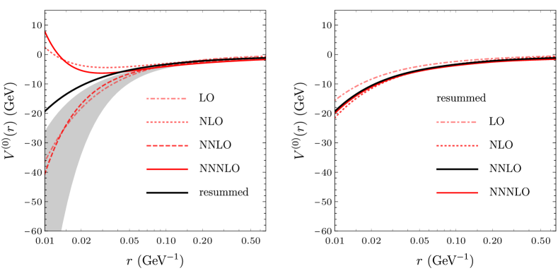
Figure 1: Left panel: perturbative QCD results for the static potential at a fixed renormalization scale $\mu_{R}=2.5$ GeV with $n_{f}=3$ at LO (dot-dashed line), NLO (dotted line), NNLO (dashed line), and NNNLO (red solid line) accuracies, compared with the resummed expression at NNLO accuracy (black solid line) given in eq. (88). The gray band shows the effect of varying the fixed renormalization scale $\mu_{R}$ between $1.5$ GeV and 4 GeV on the NNLO expression. Right panel: resummed perturbative QCD results for the static potential at the $r$-dependent renormalization scale $\mu_{r}=(r^{-2}+\mu_{R}^{2})^{1/2}$ with $n_{f}=3$ at LO (dot-dashed line), NLO (dotted line), NNLO (black solid line), and NNNLO (red solid line) accuracies. The position-space expression at NNNLO accuracy has been taken from ref. Pineda:2011dg .

We define the nonperturbative long-distance contribution to the static potential as

$$V^{(0)}(r)\big{|}_{\rm long}=\theta(r-r_{\rm match})\times\left[V^{(0)}(r)\big{|}_{\rm lattice}-V^{(0)}(r)\big{|}_{\textrm{pert, resum}}-\Delta V^{(0)}\right],$$ (89)

where $V^{(0)}(r)\big{|}_{\textrm{pert, resum}}$ is given by eq. (88), and $\Delta V^{(0)}$ is chosen so that the right-hand side vanishes at $r=r_{\rm match}$, which removes the unphysical constant shift in the lattice QCD parametrization $V^{(0)}(r)\big{|}_{\rm lattice}$. We choose $r_{\rm match}^{-1}=1.5$ GeV, which is where the slopes of $V^{(0)}(r)\big{|}_{\rm lattice}$ and $V^{(0)}(r)\big{|}_{\textrm{pert, resum}}$ are approximately same. Since $V^{(0)}(r)\big{|}_{\rm long}$ vanishes for $r<r_{\rm match}$, we obtain the following expression for the static potential that is valid for both short and long distances:

$$V^{(0)}(r)=V^{(0)}(r)\big{|}_{\textrm{pert, resum}}+V^{(0)}(r)\big{|}_{\rm long},$$ (90)

so that $V^{(0)}(r)$ coincides with the perturbative QCD expression for $r<r_{\rm match}$, while it reproduces the lattice QCD determination for $r>r_{\rm match}$. Again, the perturbative QCD expression $V^{(0)}(r)\big{|}_{\textrm{pert, resum}}$ is computed at the renormalization scale $\mu_{r}$, so that logarithms associated with the running of $\alpha_{s}$ are resummed. In fig. 2 we compare the unquenched lattice QCD results in ref. Bali:2000vr with the expression for $V^{(0)}(r)$ in eq. (90). The perturbative QCD expressions of the static potential depends on the number of light quark flavors $n_{f}$, which we take to be $n_{f}=3$ for charm, and $n_{f}=4$ for bottom. We note that the matching of perturbative QCD and lattice QCD for the pNRQCD potentials have been done in a similar way in refs. Laschka:2011zr ; Laschka:2012cf for heavy quarkonium spectroscopy.

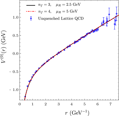
Figure 2: The static potential $V^{(0)}(r)$ including the nonperturbative long-distance contribution [eq. (90)] for $n_{f}=3$ (black solid line) and for $n_{f}=4$ (red dot-dashed line), shown with unquenched lattice QCD results from ref. Bali:2000vr , shifted vertically to match eq. (90). The renormalization scale for $\alpha_{s}$ has been chosen to be $\mu_{r}=(r^{-2}+\mu_{R}^{2})^{1/2}$, as described in text, with $\mu_{R}=2.5$ GeV for $n_{f}=3$, and $\mu_{R}=5$ GeV for $n_{f}=4$.

Eq. (90) implies that the leading-order potential is given by

$$V_{\rm LO}(r)=-\frac{\alpha_{s}(\mu_{R})C_{F}}{r}+V^{(0)}(r)\big{|}_{\rm long},$$ (91)

where in the first term on the right-hand side, $\alpha_{s}$ is evaluated at a fixed renormalization scale $\mu_{R}$. The Coulombic correction term $\delta V_{\rm C}(r)=V^{(0)}(r)-V_{\rm LO}(r)$ that appears in the second line of eq. (33) is given by

$$\delta V_{\rm C}(r)=V^{(0)}(r)\big{|}_{\textrm{pert, resum}}+\frac{\alpha_{s}(\mu_{R})C_{F}}{r},$$ (92)

where in the first term, $\alpha_{s}$ is evaluated at the scale $\mu_{r}$, while in the last term, $\alpha_{s}$ is evaluated at a fixed renormalization scale $\mu_{R}$, so that $V_{\rm LO}(r)+\delta V_{C}(r)$ reproduces the expression for $V^{(0)}(r)$ in eq. (90). The dependence on $\mu_{R}$ in $V_{\rm LO}(r)$ is cancelled explicitly by the order-$\alpha_{s}$ piece in $\delta V_{\rm C}(r)$, which is given by $-[\alpha_{s}(\mu_{r})-\alpha_{s}(\mu_{R})]C_{F}/r$. We note that $\delta V_{C}(r)$ contain contributions whose net effect is to shift the Coulomb strength of the LO potential at relative order $\alpha_{s}$, and so, the correction to the wavefunctions at the origin from $\delta V_{C}(r)$ begins at relative order $\alpha_{s}$. Although we work through first order in the QMPT, second order corrections from $\delta V_{C}(r)$ might be important, because this is of order $\alpha_{s}^{2}$. Computing the second order Coulombic correction can also be useful in testing the convergence of the Coulombic corrections. The second order Coulombic correction to the wavefunction at the origin $\Psi_{n}(0)$ can be computed by using the usual formula for the second order correction in the Rayleigh-Schrödinger perturbation theory, which reads

$$\sum_{k\neq n}\sum_{\ell\neq n}\Psi_{k}^{\rm LO}(0)\frac{\int d^{3}r_{1}d^{3}r_{2}\Psi_{k}^{\rm LO}{}^{*}({r}_{2})\delta V_{C}(r_{2})\Psi_{\ell}^{\rm LO}({r}_{2})\Psi_{\ell}^{\rm LO}{}^{*}({r}_{1})\delta V_{C}(r_{1})\Psi_{n}^{\rm LO}({r}_{1})}{(E_{n}^{\rm LO}-E_{k}^{\rm LO})(E_{n}^{\rm LO}-E_{\ell}^{\rm LO})}$$

$$-\left(\int d^{3}r\Psi_{n}^{\rm LO}{}^{*}({r})\delta V_{C}(r)\Psi_{n}^{\rm LO}({r})\right)\times\sum_{k\neq n}\Psi_{k}^{\rm LO}(0)\frac{\int d^{3}r_{1}\Psi_{k}^{\rm LO}{}^{*}({r}_{1})\delta V_{C}(r_{1})\Psi_{n}^{\rm LO}({r}_{1})}{(E_{n}^{\rm LO}-E_{k}^{\rm LO})^{2}}$$

$$-\frac{\Psi_{n}^{\rm LO}(0)}{2}\sum_{k\neq n}\frac{\left|\int d^{3}r\Psi_{k}^{\rm LO}{}^{*}({r})\delta V_{C}(r)\Psi_{n}^{\rm LO}({r})\right|^{2}}{(E_{n}^{\rm LO}-E_{k}^{\rm LO})^{2}}.$$ (93)

This expression can be rewritten in terms of the reduced Green’s functions as

$$\int d^{3}r_{1}d^{3}r_{2}\,\hat{G}_{n}(\bm{0},\bm{r}_{2})\delta V_{C}(r_{2})\hat{G}_{n}(\bm{r}_{2},\bm{r}_{1})\delta V_{C}(r_{1})\Psi_{n}^{\rm LO}(r_{1})$$ (94)

$$-\left(\int d^{3}r|\Psi_{n}^{\rm LO}(r)|^{2}\delta V_{C}(r)\right)\times\int d^{3}r_{1}d^{3}r_{2}\,\hat{G}_{n}(\bm{0},\bm{r}_{2})\hat{G}_{n}(\bm{r}_{2},\bm{r}_{1})\delta V_{C}(r_{1})\Psi_{n}^{\rm LO}(r_{1})$$

$$-\frac{\Psi_{n}^{\rm LO}(0)}{2}\int d^{3}r_{1}d^{3}r_{2}d^{3}r_{3}\,\Psi_{n}^{\rm LO}(r_{3})\delta V_{C}(r_{3})\hat{G}_{n}(\bm{r}_{3},\bm{r}_{2})\hat{G}_{n}(\bm{r}_{2},\bm{r}_{1})\delta V_{C}(r_{1})\Psi_{n}^{\rm LO}(r_{1}).\quad$$

The equivalence between the two expressions can be verified by using the identity

$$\int d^{3}r\,\hat{G}_{n}(\bm{r}_{2},\bm{r})\hat{G}_{n}(\bm{r},\bm{r}_{1})=\sum_{k\neq n}\frac{\Psi_{k}^{\rm LO}(\bm{r}_{2})\Psi_{k}^{\rm LO}{}^{*}(\bm{r}_{1})}{(E_{n}-E_{k})^{2}}.$$ (95)

In computing the second order Coulombic corrections, we neglect the $a_{2}$ term in the static potential [eq. (142)], because at second order in the QMPT, this term contributes at relative order $\alpha_{s}^{3}$.

5.1.3 $1/m$ potential from lattice QCD

We use a similar strategy as the previous section to determine the nonperturbative long-distance contribution to the $1/m$ potential. Unlike the static potential, nonperturbative determinations of the $1/m$ potential are available only from quenched lattice QCD. We use the parametrization in ref. Koma:2012bc given by

$$V^{(1)}(r)\big{|}_{\textrm{lattice}}^{\rm WL}=-\frac{9A^{2}}{8r^{2}}+\sigma^{(1)}\log r,$$ (96)

where $A=0.297$ and $\sigma^{(1)}=0.142$ GeV². This parametrization, which is based on the long-distance behavior expected from effective string theory in ref. PerezNadal:2008vm , is obtained in ref. Koma:2012bc from quenched lattice QCD results at lattice coupling $\beta=6.0$. Similarly to the lattice QCD determination of the static potential in eq. (87), only the slope in $r$ is meaningful in the lattice QCD result in eq. (96).

We match eq. (96) with the perturbative QCD expression at $r=r_{\rm match}$. Since we do not include loop corrections to the $1/m$ potential in our calculations of the wavefunctions at the origin, the expression for the $1/m$ potential $V^{(1)}(r)\big{|}_{\rm pert}^{\rm WL}$ at leading order in $\alpha_{s}$ depends on the choice of the renormalization scale. Similarly to our treatment of the static potential, we choose the renormalization scale to be $\mu_{r}=(r^{-2}+\mu_{R}^{2})^{1/2}$, so that the logarithms associated with the running of $\alpha_{s}$ are resummed, which may help smoothen the matching between the short-distance perturbative QCD expression and the nonperturbative lattice QCD parametrization at long distances. That is, we write

$$V^{(1)}(r)\big{|}_{\textrm{pert, resum}}^{\rm WL}=-\frac{\alpha_{s}^{2}(\mu_{r})C_{F}C_{A}}{2r^{2}}.$$ (97)

We compare this resummed expression with expressions at a fixed renormalization scale at LO and NLO accuracies in fig. 3.

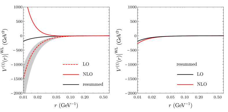
Figure 3: Left panel: perturbative QCD results for the $1/m$ potential in Wilson loop matching at a fixed renormalization scale $\mu_{R}=2.5$ GeV at LO (dashed line) and NLO (red solid line) accuracies, compared with the resummed expression at LO accuracy (black solid line) given in eq. (97). The gray band shows the effect of varying the fixed renormalization scale $\mu_{R}$ between $1.5$ GeV and 4 GeV on the LO expression. Right panel: resummed perturbative QCD results for the $1/m$ potential in Wilson loop matching at the $r$-dependent renormalization scale $\mu_{r}=(r^{-2}+\mu_{R}^{2})^{1/2}$ at LO (black solid line) and NLO (red solid line) accuracies. The position-space expression at NLO accuracy has been taken from ref. Peset:2015vvi , which is renormalized in the ${\overline{\rm MS}}$ scheme at scale 1 GeV.

We define the nonperturbative long-distance contribution to the $1/m$ potential by

$$V^{(1)}(r)\big{|}_{\textrm{long}}^{\rm WL}=\theta(r-r_{\rm match})\times\left[V^{(1)}(r)\big{|}_{\textrm{lattice}}^{\rm WL}-V^{(1)}(r)\big{|}_{\textrm{pert, resum}}^{\rm WL}-\Delta V^{(1)}\right],$$ (98)

where $\Delta V^{(1)}$ is chosen so that the right-hand side vanishes at $r=r_{\rm match}$, which removes the unphysical constant shift in the lattice QCD parametrization $V^{(1)}(r)\big{|}_{\textrm{lattice}}^{\rm WL}$. We choose $r_{\rm match}^{-1}=1.5$ GeV. Since $V^{(1)}(r)\big{|}_{\textrm{long}}^{\rm WL}$ vanishes for $r<r_{\rm match}$, we obtain an expression for the $1/m$ potential that is valid for both short and long distances given by

$$V^{(1)}(r)\big{|}^{\rm WL}=V^{(1)}(r)\big{|}_{\textrm{pert, resum}}^{\rm WL}+V^{(1)}(r)\big{|}_{\rm long}^{\rm WL}.$$ (99)

We compare the lattice QCD determination in eq. (96) with the expression for $V^{(1)}(r)\big{|}^{\rm WL}$ in eq. (99) in fig. 4.

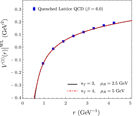
Figure 4: The $1/m$ potential $V^{(1)}(r)$ in Wilson loop matching, for $n_{f}=3$ and $\mu_{R}=2.5$ GeV (black solid line), and for $n_{f}=4$ and $\mu_{R}=5$ GeV (red dot-dashed line), shown with quenched lattice QCD results with lattice coupling $\beta=6.0$ in ref. Koma:2012bc , shifted vertically to match eq. (99).

Based on the argument given in section 4.4, we obtain the expression for the $1/m$ potential in on-shell matching that is valid for computation of wavefunctions at the origin, given by

$$V^{(1)}(r)\big{|}^{\rm OS}=\frac{\alpha_{s}^{2}(\mu_{R})C_{F}(\frac{1}{2}C_{F}-C_{A})}{2r^{2}}+V^{(1)}(r)\big{|}_{\rm long}^{\rm WL},$$ (100)

where in the first term on the right-hand side, $\alpha_{s}$ is computed at a fixed renormalization scale $\mu_{R}$. We use this form of the $1/m$ potential in the calculation of the wavefunctions at the origin.

5.1.4 Reduced Green’s function

We compute the reduced Green’s function $\hat{G}_{n}(\bm{r}^{\prime},\bm{r})$ numerically by using two different methods, which are valid in different regimes of $r$ and $r^{\prime}$. In the first method, which is valid for small $r$ and $r^{\prime}$, we compute the Green’s function in position space numerically by using the method given in ref. Strassler:1990nw . We only need to compute the $S$-wave contribution, which is defined by including only the $S$-wave states in the sum in eq. (22). This contribution can be written as

$$G^{S}(\bm{r}^{\prime},\bm{r};E)=\frac{m}{4\pi}\frac{u_{<}(r_{<})}{r_{<}}\frac{u_{>}(r_{>})}{r_{>}},$$ (101)

where $r_{<}={\rm min}(|\bm{r}|,|\bm{r}^{\prime}|)$, $r_{>}={\rm max}(|\bm{r}|,|\bm{r}^{\prime}|)$, and the superscript $S$ denotes the $S$-wave contribution. The functions $u_{<}$ and $u_{>}$ are two independent solutions of the differential equation

$$\left[\frac{d^{2}}{dr^{2}}+m(E-V_{\rm LO}(r))\right]u(r)=0,$$ (102)

with the following boundary condition

$$u_{<}(0)=0,\quad u^{\prime}_{<}(0)=1,$$ (103a)

$$u_{>}(\infty)=0,\quad u_{>}(0)=1,$$ (103b)

so that $u_{<}(r)/r$ is regular at $r=0$, while $u_{>}(r)$ is square integrable. We determine the functions $u_{<}$ and $u_{>}$ by numerically solving the differential equation for a given $E$. The reduced Green’s function can then be obtained by using the relation in eq. (25), where we take the limit numerically. We note that, if $E$ coincides with an eigenenergy of the LO Schrödinger equation $E_{n}^{\rm LO}$, then the corresponding wavefunction $\Psi_{n}^{\rm LO}(r)$ is proportional to $u_{<}(r)/r$. This means that $u_{<}(r)$ is square integrable if $E=E_{n}^{\rm LO}$, and in such case, the square-integrable solution $u_{>}(r)$ does not exist. Hence, the limit in eq. (25) must be taken with care, because the numerical solution for $u_{>}(r)$ becomes unstable if $E$ is too close to $E_{n}^{\rm LO}$. When we compute the reduced Green’s functions numerically using eq. (25), we set $\eta=10^{-3}$ GeV.

Since the first method involves computing $u_{<}(r_{<})$ by solving a differential equation with initial conditions at $r_{<}=0$, the method becomes unreliable when $r$ and $r^{\prime}$ are both large. For large $r$ and $r^{\prime}$, we compute the reduced Green’s function by using the formal solution in eq. (20), where we truncate the series by including only a limited number of the lowest eigensolutions of the LO Schrödinger equation. In the numerical calculations, we include the 9 lowest $S$-wave states in the calculation of the reduced Green’s function. This method in turn becomes unreliable at small $r$ and $r^{\prime}$. For example, if the LO potential $V_{\rm LO}(r)$ is linear in $r$ at long distances, the eigenenergies of highly excited $S$-wave states increase linearly with increasing principal quantum number, and the LO wavefunctions at the origin are constant in the principal quantum number. Hence, the series in eq. (20) diverges like $\sum_{n}^{\infty}1/n$ at $r=r^{\prime}=0$. This implies that the truncated series becomes unreliable at small $r$ and $r^{\prime}$.

We combine the reduced Green’s function at long and short distances by

$$\hat{G}_{n}(\bm{r}^{\prime},\bm{r})=b(r_{<})\times\hat{G}_{n}(\bm{r}^{\prime},\bm{r})|_{\rm short}+\left[1-b(r_{<})\right]\times\hat{G}_{n}(\bm{r}^{\prime},\bm{r})|_{\rm long},$$ (104)

where $\hat{G}_{n}(\bm{r}^{\prime},\bm{r})|_{\rm short}$ is computed by using eqs. (101) and (25), $\hat{G}_{n}(\bm{r}^{\prime},\bm{r})|_{\rm long}$ is computed by truncating the series in eq. (20), and $b(r)$ is a smooth function that satisfies $b(0)=1$ and $b(\infty)=0$, so that eq. (104) is reliable for all $r$ and $r^{\prime}$. We define $b(r)$ by

$$b(r)=\frac{1}{\pi}\left[\tan^{-1}(4m(r_{b}-r))-\tan^{-1}(4mr_{b})\right]+1,$$ (105)

with $r_{b}=1$ GeV^-1. The validity of the reduced Green’s function obtained in eq. (104) can be tested by numerically checking the relations

$$\left(E_{k}^{\rm LO}-E_{n}^{\rm LO}\right)\int d^{3}r\,\hat{G}_{n}(\bm{r}^{\prime},\bm{r})\Psi_{k}^{\rm LO}(r) = \Psi_{k}^{\rm LO}(r^{\prime}),$$ (106a)

$$\int d^{3}r\,\hat{G}_{n}(\bm{r}^{\prime},\bm{r})\Psi_{n}^{\rm LO}(r) = 0,$$ (106b)

for $k\neq n$.

We note that, due to the boundary condition $u_{>}(0)=1$, it is evident that $G^{S}(\bm{0},\bm{r};E)$ develops a power divergence given by $m/(4\pi r)$ near $r=0$. It has been shown in ref. Kiyo:2010jm that if the LO potential is given by $V_{\rm LO}(r)=-\alpha_{s}C_{F}/r$ at short distances, $u_{>}(r)/r$ also contains a logarithmic divergence given by $-\alpha_{s}C_{F}m\log r$. Therefore, near $r=0$, the Green’s function behaves like

$$G^{S}(\bm{0},\bm{r};E)=\frac{m}{4\pi r}-\frac{\alpha_{s}C_{F}m^{2}}{4\pi}\log r+\cdots,$$ (107)

where the ellipsis represent contributions that are finite at $r=0$. This shows that the divergent small $r$ behavior of $G^{S}(\bm{0},\bm{r};E)$ depends only on the short-distance behavior of the LO potential, which is determined in perturbative QCD.

5.1.5 Gluonic correlators

The pNRQCD expressions of the NRQCD LDMEs in eqs. (10) and (13) depend on gluonic correlators that scale with powers of $\Lambda_{\rm QCD}$. Also, corrections to the wavefunctions at the origin from the velocity-dependent potential involve $V_{p^{2}}^{(2)}(0)$, which in DR, is proportional to the correlator $i{\cal E}_{2}$. While the gluonic correlators of mass dimension two contribute to the NRQCD LDMEs at relative order $\Lambda_{\rm QCD}^{2}/m^{2}$, the dimensionless correlator ${\cal E}_{3}$ contributes to $\langle 0|\chi^{\dagger}\bm{\epsilon}\cdot\bm{\sigma}\psi|V\rangle$ and $\langle 0|\chi^{\dagger}\psi|P\rangle$ at relative order $v^{2}$, and the correlator $i{\cal E}_{2}$ contributes to the wavefunctions at the origin at relative order $\Lambda_{\rm QCD}/m$.

The dimensionless correlator ${\cal E}_{3}$ in the $\overline{\rm MS}$ scheme has been determined in ref. Brambilla:2020xod from measured decay rates of $P$-wave charmonia. At the $\overline{\rm MS}$ scale $\Lambda=1$ GeV,

$${\cal E}_{3}(1\textrm{~{}GeV})=2.05^{+0.94}_{-0.65}.$$ (108)

The correlator ${\cal E}_{3}$ depends logarithmically on the scale. We compute ${\cal E}_{3}$ at other scales by using the one-loop renormalization group improved expression Brambilla:2001xy ; Brambilla:2020xod

$${\cal E}_{3}(\Lambda)={\cal E}_{3}(\Lambda^{\prime})+\frac{24C_{F}}{\beta_{0}}\log\frac{\alpha_{s}(\Lambda^{\prime})}{\alpha_{s}(\Lambda)}.$$ (109)

Reference Brambilla:2020xod also provides a determination of $i{\cal E}_{2}$ from measured electromagnetic decay and production rates of $P$-wave charmonia. However, the determination in ref. Brambilla:2020xod has uncertainties that are larger than the typical size of the correlator that is expected from its power counting. For this reason, instead of taking the determination in ref. Brambilla:2020xod , we consider the effect of $V_{p^{2}}^{(2)}(0)$ to the wavefunctions at the origin in the uncertainties by assuming $|V_{p^{2}}^{(2)}|\lesssim 500$ MeV, which corresponds to the typical size of $\Lambda_{\rm QCD}$.

Since the gluonic correlators of mass dimension two contribute to the NRQCD LDMEs at relative order $\Lambda_{\rm QCD}^{2}/m^{2}$, we neglect them in calculations of the LDMEs compared to corrections of relative order $\Lambda_{\rm QCD}/m$ and $v^{2}$.

5.2 Numerical results for $S$-wave charmonia

In this section, we compute the $\overline{\rm MS}$-renormalized wavefunctions at the origin for the $1S$ and $2S$ charmonium states. We identify the $J/\psi$ and $\eta_{c}$ as the $1S$ charmonium states in spin-triplet and spin-singlet states, respectively, while the $\psi(2S)$ and $\eta_{c}(2S)$ states are the $2S$ charmonium states in spin-triplet and spin-singlet states, respectively.

As we discussed in previous sections, we solve the Schrödinger equation numerically with the LO potential in eq. (91) and the charm quark mass in eq. (86a) to determine $\Psi_{n}^{\rm LO}(r)$, $E_{n}^{\rm LO}$, and $\hat{G}_{n}(\bm{r}^{\prime},\bm{r})$. For this purpose, it suffices to solve the differential equation in eq. (102) and obtain the solutions $u_{<}(r)$ and $u_{>}(r)$ for a range of $E$, because $u_{<}(r)$ becomes square integrable when $E=E_{n}^{\rm LO}$, and the corresponding eigenfunction $\Psi_{n}^{\rm LO}(r)$ is then proportional to $u_{<}(r)/r$. We obtain the solution $u_{<}(r)$ by solving the differential equation in eq. (102) numerically in Mathematica using the NDSolve command with the initial conditions $u_{<}(0)=0$ and $u^{\prime}_{<}(0)=1$. Instead of obtaining directly the $u_{>}(r)$ with the boundary conditions $u_{>}(0)=1$ and $u_{>}(\infty)=0$, we find a linearly independent second solution $v(r)$ which is in general a linear combination of $u_{<}(r)$ and $u_{>}(r)$. Similarly to what has been done in ref. Kiyo:2010jm , we find a solution $v(r)$ that satisfies $v(0)=1$, and let $v^{\prime}(r)$ be nonzero at small $r$ (in general $v^{\prime}(r)$ is singular at $r=0$ Strassler:1990nw ; Kiyo:2010jm ). Then, the solution $u_{>}(r)$ that satisfies the boundary conditions $u_{>}(0)=1$ and $u_{>}(\infty)=0$ is given by $u_{>}(r)=v(r)-\frac{v(\infty)}{u_{<}(\infty)}u_{<}(r)$.

Then, we compute the corrections to the wavefunctions at the origin in the finite-$r$ regularization using eq. (33). In order to compensate for the use of the $\rm RS^{\prime}$ mass, we add to eq. (33) the finite correction from the $\rm RS^{\prime}$ subtraction term in eq. (85). We also add to eq. (33) the Coulombic correction at second order in QMPT in eq. (94). In the calculation of the corrections to the wavefunctions at the origin, we use the $1/m$ potential given by eq. (100), while we take the perturbative QCD expressions of the $1/m^{2}$ potentials given by eq. (144). When we compute the central values of the wavefunctions at the origin, we set $V_{p^{2}}^{(2)}(0)=0$ in eq. (33), and consider the effect of the correction from $V_{p^{2}}^{(2)}(0)$ in the uncertainties. We then use eq. (34) to obtain the $\overline{\rm MS}$-renormalized wavefunctions at the origin.

In computing the finite-$r$ regularized wavefunctions at the origin, the regulator $r_{0}$ must be chosen to be as small as possible, as long as the numerical calculation is stable. We determine an optimal choice of $r_{0}$ by numerically testing the approximate relation in eq. (77). We find that the relation is well reproduced numerically at $1\%$ level for $r_{0}\gtrsim 0.1$ GeV^-1. Hence, we choose $r_{0}=0.2$ GeV^-1, and vary $r_{0}$ between $0.1$ GeV^-1 and $0.3$ GeV^-1. We set the $\overline{\rm MS}$ scale $\Lambda$ to be the charm quark mass $m$, and choose the central value of the QCD renormalization scale $\mu_{R}$ to be 2.5 GeV, as discussed in sec. 5.1.1.

We list the central values of the LO wavefunctions at the origin and the LO binding energies in table 1. We also list the corrections to the wavefunctions at the origin relative to $\Psi_{n}^{\rm LO}(0)$ in table 1. We classify the corrections by their origins in the following way: the non-Coulombic correction $\delta_{\Psi}^{\rm NC}$ comes from the $1/m$ and $1/m^{2}$ potentials, the Coulombic corrections $\delta_{\Psi}^{\rm C1}$ and $\delta_{\Psi}^{\rm C2}$ come from $\delta V_{C}(r)$ at first and second order in the QMPT, respectively, and the correction $\delta_{\Psi}^{\rm RS^{\prime}}$ comes from the $\rm RS^{\prime}$ subtraction term. The explicit expressions for $\delta_{\Psi}^{\rm NC}$ and $\delta_{\Psi}^{\rm C1}$ are given by

$$\delta_{\Psi}^{\rm NC} = -\delta Z-\frac{1}{\Psi_{n}^{\rm LO}(0)}\int d^{3}r\,\hat{G}_{n}(\bm{r}^{\prime},\bm{r})\delta{\cal V}(r)\Psi_{n}^{\rm LO}(r)\Big{|}_{|\bm{r}^{\prime}|=r_{0}}$$ (110a)

$$-\frac{1}{\Psi_{n}^{\rm LO}(0)}\frac{E_{n}^{\rm LO}}{m}\int d^{3}r\,\hat{G}_{n}(\bm{0},\bm{r})\left[V_{p^{2}}^{(2)}(r)+\frac{1}{2}V_{\rm LO}(r)\right]\Psi_{n}^{\rm LO}(r)$$

$$+\frac{1}{2m}\int d^{3}r\,\left[V_{p^{2}}^{(2)}(r)+\frac{1}{2}V_{\rm LO}(r)\right]\left|\Psi_{n}^{\rm LO}(r)\right|^{2}-\frac{V_{p^{2}}^{(2)}(0)}{2m},$$

$$\delta_{\Psi}^{\rm C1} = -\frac{1}{\Psi_{n}^{\rm LO}(0)}\int d^{3}r\,\hat{G}_{n}(\bm{0},\bm{r})\delta V_{C}(r)\Psi_{n}^{\rm LO}(r),$$ (110b)

while $\delta_{\Psi}^{\rm C2}$ is given by dividing eq. (94) by $\Psi_{n}^{\rm LO}(0)$, and $\delta_{\Psi}^{\rm RS^{\prime}}$ is given by dividing eq. (85) by $\Psi_{n}^{\rm LO}(0)$. The $\overline{\rm MS}$-renormalized wavefunctions at the origin are then given by

$$\Psi_{n}(0)|_{\overline{\rm MS}}=\Psi_{n}^{\rm LO}(0)\times\left(1+\delta_{\Psi}^{\rm NC}+\delta_{\Psi}^{\rm C1}+\delta_{\Psi}^{\rm C2}+\delta_{\Psi}^{\rm RS^{\prime}}\right).$$ (111)

We note that the $r_{0}$ dependence cancels in $\delta_{\Psi}^{\rm NC}$ between $\delta Z$ and the finite-$r$ regularized integral for small $r_{0}$. We demonstrate this cancellation of the $r_{0}$ dependence in fig. 5.

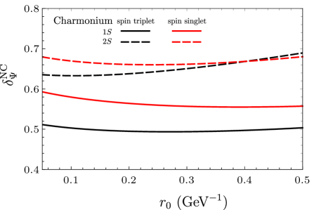
Figure 5: The non-Coulombic corrections $\delta_{\Psi}^{\rm NC}$ at finite $r_{0}$ for the charmonium $1S$ (solid lines) and $2S$ (dashed lines) states, for spin triplet (black) and spin singlet (red). The $r_{0}$ dependences are mild for the range 0.1 GeV${}^{-1}<r_{0}<$ 0.3 GeV^-1 that we consider.

State	$\Psi^{\rm LO}(0)$ (GeV3/2)	$E^{\rm LO}$ (GeV)	$\delta_{\Psi}^{\rm NC}|_{\bm{S}^{2}=2}$	$\delta_{\Psi}^{\rm NC}|_{\bm{S}^{2}=0}$	$\delta_{\Psi}^{\rm C1}$	$\delta_{\Psi}^{\rm C2}$	$\delta_{\Psi}^{\rm RS^{\prime}}$
$1S$	0.183	0.233	0.495	0.564	0.173	$-0.010$	0.080
$2S$	0.177	0.769	0.638	0.661	0.079	$-0.004$	0.072

Table 1: LO wavefunctions at the origin, LO binding energies and relative corrections to the wavefunctions at the origin in the $\overline{\rm MS}$ scheme at scale $\Lambda=m$ for $1S$ and $2S$ charmonium states. $\delta_{\Psi}^{\rm NC}$ is the correction from the $1/m$ and $1/m^{2}$ potentials, $\delta_{\Psi}^{\rm C1}$ and $\delta_{\Psi}^{\rm C2}$ are Coulombic corrections at first and second order in QMPT, respectively, and $\delta_{\Psi}^{\rm RS^{\prime}}$ is the correction from the $\rm RS^{\prime}$ subtraction term. The $\delta_{\Psi}^{\rm NC}$, $\delta_{\Psi}^{\rm C1}$, $\delta_{\Psi}^{\rm C2}$, and $\delta_{\Psi}^{\rm RS^{\prime}}$ are dimensionless.

The results for the LO binding energies for the $1S$ and $2S$ states in table 1 are roughly compatible with the mass difference between $J/\psi$ and $\psi(2S)$. We see that the non-Coulombic corrections from $1/m$ and $1/m^{2}$ potentials, given by $\delta_{\Psi}^{\rm NC}$ in table 1, are large and positive for both $1S$ and $2S$ states. This is in contrast with the order-$\alpha_{s}^{2}$ corrections to the NRQCD SDCs in appendix C, which are large and negative at $\Lambda=m$. This implies that if we combine the pNRQCD expressions of the LDMEs with the NRQCD SDCs, large cancellations will occur between the order-$\alpha_{s}^{2}$ corrections to the SDCs and the corrections to the wavefunctions at the origin. The contribution from the long-distance part of the $1/m$ potential, which is given by the second term in eq. (100), amounts to about $+10\%$ of the LO wavefunction at the origin for the $1S$ state, and about $+6\%$ of the LO wavefunction at the origin for the $2S$ state. We note that while the Coulombic corrections at first order are positive, the Coulombic corrections at second order are small and negative, signaling good convergence of the Coulombic corrections. The corrections from the renormalon subtraction term $\delta_{\Psi}^{\rm RS^{\prime}}$ are mild for both $1S$ and $2S$ states.

The LO wavefunctions at the origin in table 1 are much larger than what we would obtain if we neglect the long-distance nonperturbative part of the static potential, for example, by using the analytical solution of the Schrödinger equation in perturbative QCD (see appendix D). For the $1S$ state, neglecting the long-distance nonperturbative part of the static potential reduces the wavefunction at the origin by more than a factor of 2, and for the $2S$ state, the wavefunction at the origin reduces by more than a factor of 7. At the squared amplitude level, neglecting the long-distance part of the static potential can reduce the $1S$ charmonium decay rates by almost an order of magnitude, and $2S$ charmonium decay rates by more than an order of magnitude. Hence, the long-distance nonperturbative part of the static potential has a significant effect on charmonium wavefunctions at the origin and charmonium decay rates.

We use the results for the $\overline{\rm MS}$ wavefunctions at the origin in table 1 to compute decay constants and electromagnetic decay rates of $S$-wave charmonium states. We first compute the decay constants $f_{V}$ of $V=J/\psi$ and $\psi(2S)$. By using the pNRQCD expressions of the LDMEs in eqs. (10) and (12) and the SDCs in appendix C, and expanding the corrections to the SDCs and to the wavefunctions at the origin, we obtain

$$f_{V} = \sqrt{\frac{4N_{c}}{m_{V}}}\Psi_{V}^{\rm LO}(0)\bigg{[}1+\alpha_{s}c_{v}^{(1)}+\delta_{\Psi}^{\rm C1}+\delta_{\Psi}^{\rm C2}+\delta_{\Psi}^{\rm RS^{\prime}}+\delta_{\Psi}^{\rm NC}|_{\bm{S}^{2}=2}+\alpha_{s}^{2}c_{v}^{(2)}$$ (112)

$$\hskip 68.88867pt+\alpha_{s}c_{v}^{(1)}\delta_{\Psi}^{\rm C1}+\frac{2E_{V}^{\rm LO}}{m_{V}}\left(d_{v}-\frac{{\cal E}_{3}}{9}\right)+O(\alpha_{s}^{3},v^{3},\Lambda_{\rm QCD}^{2}/m^{2})\bigg{]},\quad$$

where $c_{v}=1+\alpha_{s}c_{v}^{(1)}+\alpha_{s}^{2}c_{v}^{(2)}+O(\alpha_{s}^{3})$, and $\alpha_{s}=\alpha_{s}(\mu_{R})$. This expression is valid up to corrections of relative order $\alpha_{s}^{3}$, $v^{3}$, and $\Lambda_{\rm QCD}^{2}/m^{2}$. We set $n_{f}=3$ in the SDCs. Since we assume $\delta_{\Psi}^{\rm C1}$ to be of order $\alpha_{s}$, we keep the cross term $\alpha_{s}c_{v}^{(1)}\delta_{\Psi}^{\rm C1}$. The dependence on the $\overline{\rm MS}$ scale $\Lambda$ in $\delta_{\Psi}^{\rm NC}|_{\bm{S}^{2}=2}$ cancels completely with the $\Lambda$ dependence in $\alpha_{s}^{2}c_{v}^{(2)}$, while the $\Lambda$ dependence in the order-$\alpha_{s}$ correction to $d_{v}$ cancels with the scale dependence of the correlator ${\cal E}_{3}$. Hence, variation of the factorization scale $\Lambda$ has almost no effect in eq. (112). We set the scale $\Lambda=m$ in the one-loop correction to $d_{v}$, and compute the correlator ${\cal E}_{3}$ at the same scale using the renormalization group improved expression in eq. (109). We take the measured quarkonium masses from ref. Tanabashi:2018oca .

The numerical result for the $J/\psi$ decay constant is

$$f_{J/\psi}=0.363{}^{+0.015}_{-0.003}{}^{+0.003}_{-0.000}\pm 0.069\pm 0.054\textrm{~{}GeV}=0.363{}^{+0.089}_{-0.088}\textrm{~{}GeV},$$ (113)

where the first uncertainty comes from varying $\mu_{R}$ between $1.5$ GeV and $4$ GeV, and the second uncertainty comes from varying $r_{0}$ between 0.1 GeV^-1 and 0.3 GeV^-1. The third uncertainty comes from the neglect of the correction $-V_{p^{2}}^{(2)}(0)/(2m)$ to the wavefunction at the origin, which we take to be $\pm 500\textrm{~{}MeV}/(2m)$ times the central value. The last uncertainty comes from the uncalculated corrections of order $v^{3}$, which we take to be 15% of the central value, based on the typical estimate $v^{2}\approx 0.3$ for charmonium states. In the last equality, we add the uncertainties in quadrature.

We note that the central value for $f_{J/\psi}$ that we obtain is very close to the leading-order value $f_{J/\psi}^{\rm LO}=0.360$ GeV. The order-$\alpha_{s}$ terms in eq. (112) from $\alpha_{s}c_{v}^{(1)}$ and $\delta_{\Psi}^{\rm C1}$ amount to about $-6\%$ of the central value, and the corrections proportional to $E_{V}^{\rm LO}$ is about $-7\%$ of the central value. The remaining corrections from $\alpha_{s}^{2}c_{v}^{(2)}$, $\delta_{\Psi}^{\rm NC}$, $\delta_{\Psi}^{\rm C2}$, $\delta_{\Psi}^{\rm RS^{\prime}}$, and the cross term $\alpha_{s}c_{v}^{(1)}\delta_{\Psi}^{\rm C1}$ add up to about $+14\%$ of the central value, so that the numerical result for $f_{J/\psi}$ in eq. (113) is only about $1\%$ larger than the leading-order value. If we had ignored the corrections to the wavefunctions at the origin, the one-loop correction would have been $-23\%$ of the leading order result, while the two-loop correction would have been $-39\%$ of the leading order value, so that the loop corrections add up to $-62\%$ at two-loop accuracy. The inclusion of the corrections to the wavefunction at the origin in the calculation of the decay constant $f_{J/\psi}$ has substantially improved the convergence of the expansion in $\alpha_{s}$ and $v$.

The result for $f_{J/\psi}$ agrees within uncertainties with the lattice QCD determination using relativistic charm quarks in ref. Hatton:2020qhk , which gives $f_{J/\psi}=0.4104(17)$ GeV. In order to compare with measurements, we compute the leptonic decay rate of $J/\psi$ from $f_{J/\psi}$ by using eq. (82). We obtain

$$\Gamma(J/\psi\to e^{+}e^{-})=4.5{}^{+2.5}_{-1.9}\textrm{~{}keV},$$ (114)

where we used $\alpha=1/133$, which is computed at the scale of the $J/\psi$ mass. This result agrees with the experimental value $\Gamma(J/\psi\to e^{+}e^{-})=5.53\pm 0.10$ keV in ref. Tanabashi:2018oca within uncertainties.

The leptonic decay rate can also be computed by using the NRQCD factorization formula at the decay rate level, which is obtained by squaring the amplitude-level factorization formula (147), and expanding in powers of $\alpha_{s}$ and $v$. In order to facilitate exact order-by-order cancellation of the NRQCD factorization scale dependence, we also expand the pNRQCD expressions for the NRQCD LDMEs at the squared amplitude level, as well as the square of the wavefunction at the origin in powers of $\alpha_{s}$, $v$, and $\Lambda_{\rm QCD}/m$. That is, we square the expression for the decay constant in eq. (112) and then expand the corrections in powers of $\alpha_{s}$, $v$, and $\Lambda_{\rm QCD}/m$. In this case, we obtain $\Gamma(J/\psi\to e^{+}e^{-})=4.5^{+1.9}_{-1.8}$ keV, which agrees well with the result in eq. (114) within uncertainties. This agreement is due to the fact that the convergence of the expansion in powers of $\alpha_{s}$, $v$, and $\Lambda_{\rm QCD}/m$ have improved significantly in both the decay constant and the leptonic decay rate, thanks to the corrections to the wavefunctions at the origin that we have included.

The numerical result for the $\psi(2S)$ decay constant is

$$f_{\psi(2S)}=0.309{}^{+0.011}_{-0.010}{}^{+0.004}_{-0.002}\pm 0.059\pm 0.046\textrm{~{}GeV}=0.309{}^{+0.076}_{-0.076}\textrm{~{}GeV},$$ (115)

where the uncertainties are as in eq. (113). Again, the central value for $f_{\psi(2S)}$ that we obtain is very close to the leading-order value $f_{\psi(2S)}^{\rm LO}=0.318$ GeV. This follows from the improvement of the convergence of the corrections of higher orders in $\alpha_{s}$ and $v$ by the inclusion of the corrections to the wavefunction at the origin. We compute the leptonic decay rate of $\psi(2S)$ by using eq. (82). We obtain

$$\Gamma(\psi(2S)\to e^{+}e^{-})=2.7{}^{+1.5}_{-1.2}\textrm{~{}keV},$$ (116)

where we used $\alpha=1/133$, which is computed at the scale of the $\psi(2S)$ mass. This result agrees with the experimental value $\Gamma(\psi(2S)\to e^{+}e^{-})=2.33\pm 0.04$ keV in ref. Tanabashi:2018oca within uncertainties. If we use the expression for the decay rate expanded in powers of $\alpha_{s}$, $v$, and $\Lambda_{\rm QCD}/m$ at the squared amplitude level, we obtain $\Gamma(\psi(2S)\to e^{+}e^{-})=2.7\pm 1.1$ keV, which agrees well within uncertainties with eq. (116).

Now we compute the decay constants $f_{P}$ of $P=\eta_{c}$ and $\eta_{c}(2S)$. Although $f_{P}$ cannot be obtained directly from experimental measurements, this decay constant appears in exclusive production cross sections of pseudoscalar quarkonia at high energies Jia:2008ep ; Chung:2019ota . We obtain the following expression for $f_{P}$ by expanding the corrections to the SDCs and the corrections to the wavefunctions at the origin:

$$f_{P} = \sqrt{\frac{4N_{c}}{m_{P}}}\Psi_{P}^{\rm LO}(0)\bigg{[}1+\alpha_{s}c_{p}^{(1)}+\delta_{\Psi}^{\rm C1}+\delta_{\Psi}^{\rm C2}+\delta_{\Psi}^{\rm RS^{\prime}}+\delta_{\Psi}^{\rm NC}|_{\bm{S}^{2}=0}+\alpha_{s}^{2}c_{p}^{(2)}$$ (117)

$$\hskip 68.88867pt+\alpha_{s}c_{p}^{(1)}\delta_{\Psi}^{\rm C1}+\frac{2E_{P}^{\rm LO}}{m_{P}}\left(d_{p}-\frac{{\cal E}_{3}}{9}\right)+O(\alpha_{s}^{3},v^{3},\Lambda_{\rm QCD}^{2}/m^{2})\bigg{]},$$

where $c_{p}=1+\alpha_{s}c_{p}^{(1)}+\alpha_{s}^{2}c_{p}^{(2)}+O(\alpha_{s}^{3})$, and $\alpha_{s}=\alpha_{s}(\mu_{R})$. We neglect the small imaginary part in $c_{p}^{(2)}$, which amounts to less than $0.02$. This expression is valid up to corrections of relative order $\alpha_{s}^{3}$, $v^{3}$, and $\Lambda_{\rm QCD}^{2}/m^{2}$. We set $n_{f}=3$ in the SDCs. We note that the $\Lambda$ dependence in $\delta_{\Psi}^{\rm NC}|_{\bm{S}^{2}=0}$ cancels exactly with $\alpha_{s}^{2}c_{p}^{(2)}$. Since the order-$\alpha_{s}$ correction to $d_{p}$ is not available, our expression for $f_{P}$ in eq. (117) depends mildly on $\Lambda$ through the scale dependence of ${\cal E}_{3}$. Nevertheless, variation of the factorization scale $\Lambda$ has a very small effect in eq. (117). We compute ${\cal E}_{3}$ at the scale $\Lambda=m$. We take the measured quarkonium masses from ref. Tanabashi:2018oca .

The numerical result for $f_{\eta_{c}}$ is

$$f_{\eta_{c}}=0.385{}^{+0.013}_{-0.000}{}^{+0.006}_{-0.003}\pm 0.073\pm 0.057\textrm{~{}GeV}=0.385{}^{+0.094}_{-0.093}\textrm{~{}GeV},$$ (118)

where the uncertainties are as in eq. (113). We add the uncertainties in quadrature. We neglect the uncertainty from the scale dependence of ${\cal E}_{3}$, which is small compared to other uncertainties. This result for $f_{\eta_{c}}$ agrees with the lattice QCD determination using relativistic charm quarks in refs. Hatton:2020qhk , which gives $f_{\eta_{c}}=0.3981(10)$ MeV.

Similarly to the case of $f_{J/\psi}$, the central value for $f_{\eta_{c}}$ that we obtain is very close to the leading-order value $f_{\eta_{c}}^{\rm LO}=0.367$ GeV. The order-$\alpha_{s}$ corrections in eq. (117) from $\alpha_{s}c_{p}^{(1)}$ and $\delta_{\Psi}^{\rm C1}$ amount to about $1\%$ of the central value, and the corrections proportional to $E_{P}^{\rm LO}$ is about $-13\%$ of the central value. The remaining corrections from $\alpha_{s}^{2}c_{v}^{(2)}$, $\delta_{\Psi}^{\rm NC}$, $\delta_{\Psi}^{\rm C2}$, $\delta_{\Psi}^{\rm RS^{\prime}}$, and the cross term $\alpha_{s}c_{v}^{(1)}\delta_{\Psi}^{\rm C1}$ add up to about $+17\%$ of the central value, so that the central value for $f_{\eta_{c}}$ in eq. (118) is only about $4\%$ larger than the leading-order value. In contrast, if we had ignored the corrections to the wavefunctions at the origin, the one-loop correction would have been $-16\%$ of the leading order result, while the two-loop correction would have been $-44\%$ of the leading order value, so that the loop corrections add up to $-60\%$ at two-loop accuracy. Just like the case of the $J/\psi$ and $\psi(2S)$ decay constants, the inclusion of the corrections to the wavefunction at the origin in the calculation of the decay constant $f_{\eta_{c}}$ greatly improves the convergence of the expansion in $\alpha_{s}$ and $v$.

The numerical result for $f_{\eta_{c}(2S)}$ is

$$f_{\eta_{c}(2S)}=0.275{}^{+0.010}_{-0.019}{}^{+0.003}_{-0.000}\pm 0.052\pm 0.041\textrm{~{}GeV}=0.271{}^{+0.068}_{-0.069}\textrm{~{}GeV},$$ (119)

where the uncertainties are as in eq. (118). For the case of $\eta_{c}(2S)$, the central value for $f_{\eta_{c}(2S)}$ that we obtain is about $18\%$ smaller than the leading-order value $f_{\eta_{c}(2S)}^{\rm LO}=0.321$ GeV. The difference is larger than the case of $\eta_{c}$, because the binding energy of the $2S$ state is larger than the binding energy of the $1S$ state, and so, the correction proportional to $E^{\rm LO}_{\eta_{c}(2S)}$ is larger compared to the $\eta_{c}$ case.

Finally, we compute the two-photon decay rate of $P=\eta_{c}$ and $\eta_{c}(2S)$. The NRQCD factorization formula for the decay rate is given in appendix C. The following expression for the decay rate is obtained by expanding the corrections to the SDCs and the corrections to the wavefunctions at the origin at the amplitude level:

$$\Gamma(P\to\gamma\gamma) = \frac{16N_{c}\pi\alpha^{2}e_{Q}^{4}}{m_{P}^{2}}|\Psi_{P}^{\rm LO}(0)|^{2}\bigg{|}\bigg{[}1+\alpha_{s}c_{\gamma\gamma}^{(1)}+\delta_{\Psi}^{\rm C1}+\delta_{\Psi}^{\rm C2}+\delta_{\Psi}^{\rm RS^{\prime}}+\delta_{\Psi}^{\rm NC}|_{\bm{S}^{2}=0}$$ (120)

$$+\alpha_{s}^{2}c_{\gamma\gamma}^{(2)}+\alpha_{s}c_{\gamma\gamma}^{(1)}\delta_{\Psi}^{\rm C1}+\frac{2E_{P}^{\rm LO}}{m_{P}}\left(d_{\gamma\gamma}-\frac{{\cal E}_{3}}{9}\right)+O(\alpha_{s}^{3},v^{3},\Lambda_{\rm QCD}^{2}/m^{2})\bigg{]}\bigg{|}^{2},\quad\quad$$

where $c_{\gamma\gamma}=1+\alpha_{s}c_{\gamma\gamma}^{(1)}+\alpha_{s}^{2}c_{\gamma\gamma}^{(2)}+O(\alpha_{s}^{3})$, and $\alpha_{s}=\alpha_{s}(\mu_{R})$. This expression is valid up to corrections of relative order $\alpha_{s}^{3}$, $v^{3}$, and $\Lambda_{\rm QCD}^{2}/m^{2}$. We set $n_{f}=3$ in the SDCs, and use $e_{Q}=2/3$ for charm. We choose $\alpha=1/137$, because the QED coupling constant in eq. (120) is associated with on-shell photons in the final state. The dependence on the $\overline{\rm MS}$ scale $\Lambda$ in $\delta_{\Psi}^{\rm NC}|_{\bm{S}^{2}=0}$ cancels completely with the $\Lambda$ dependence in $\alpha_{s}^{2}c_{\gamma\gamma}^{(2)}$, while the $\Lambda$ dependence in the order-$\alpha_{s}$ correction to $d_{\gamma\gamma}$ cancels with the scale dependence of the correlator ${\cal E}_{3}$. Similarly to the case of decay constants, variation of the factorization scale $\Lambda$ has almost no effect in eq. (120). We set the scale $\Lambda=m$ in the one-loop correction to $d_{\gamma\gamma}$, and compute the correlator ${\cal E}_{3}$ at scale $m$ using the renormalization group improved expression in eq. (109).

The numerical result for the two-photon decay rate of $\eta_{c}$ is

$$\Gamma(\eta_{c}\to\gamma\gamma)=6.8{}^{+0.4}_{-0.0}{}^{+0.2}_{-0.1}{}^{+2.8}_{-2.3}\pm 1.0\textrm{~{}keV}=6.8{}^{+3.0}_{-2.5}\textrm{~{}keV},$$ (121)

where the uncertainties are as in eq. (113). This result is compatible within uncertainties with the PDG value of the two-photon decay rate $\Gamma(\eta_{c}\to\gamma\gamma)=5.06\pm 0.34$ keV in ref. Tanabashi:2018oca . The central value for the decay rate that we obtain is not very different from the leading-order value $\Gamma(\eta_{c}\to\gamma\gamma)|^{\rm LO}=16N_{c}\pi\alpha^{2}e_{Q}^{4}|\Psi_{\eta_{c}}^{\rm LO}(0)|^{2}/m_{\eta_{c}}^{2}=6.0$ keV. If we had ignored the corrections to the wavefunctions at the origin, the one-loop correction would have been $-15\%$ of the leading order result at the amplitude level, while the two-loop correction would have been $-46\%$ of the leading order amplitude, so that the effect of the loop corrections would add up to $-61\%$ at two-loop accuracy at the amplitude level. In contrast, the order-$\alpha_{s}$ corrections in eq. (120) from $\alpha_{s}c_{\gamma\gamma}^{(1)}$ and $\delta_{\Psi}^{\rm C1}$ amount to about $3\%$, and the corrections proportional to $E_{\eta_{c}}^{\rm LO}$ is about $-10\%$ compared to the leading-order amplitude. The remaining corrections from $\alpha_{s}^{2}c_{v}^{(2)}$, $\delta_{\Psi}^{\rm NC}$, $\delta_{\Psi}^{\rm C2}$, $\delta_{\Psi}^{\rm RS^{\prime}}$, and the cross term $\alpha_{s}c_{v}^{(1)}\delta_{\Psi}^{\rm C1}$ add up to about $+14\%$ of the leading-order amplitude, so that the central value for the decay rate that we obtain is about $7\%$ larger than the leading-order value at the amplitude level, or about $13\%$ larger at the squared amplitude level. Inclusion of the corrections to the wavefunctions at the origin in eq. (120) has improved the convergence of the corrections of higher orders in $\alpha_{s}$ and $v$. If we compute the decay rate by expanding the expression in eq. (120) at the squared amplitude level, as we have done for the leptonic decay rates of $J/\psi$ and $\psi(2S)$, we obtain $\Gamma(\eta_{c}\to\gamma\gamma)=6.7^{+3.0}_{-2.5}$ keV, which agrees well with eq. (121) within uncertainties.

The numerical result for the two-photon decay rate of $\eta_{c}(2S)$ is

$$\Gamma(\eta_{c}(2S)\to\gamma\gamma)=3.0{}^{+0.4}_{-0.7}{}^{+0.1}_{-0.0}{}^{+1.3}_{-1.0}\pm 0.6\textrm{~{}keV}=3.0{}^{+1.4}_{-1.3}\textrm{~{}keV},$$ (122)

where the uncertainties are as in eq. (113). The central value of the decay rate is about $19\%$ smaller than the leading-order value $\Gamma(\eta_{c}(2S)\to\gamma\gamma)|^{\rm LO}=16N_{c}\pi\alpha^{2}e_{Q}^{4}|\Psi_{\eta_{c}(2S)}^{\rm LO}(0)|^{2}/m_{\eta_{c}(2S)}^{2}=3.7$ keV. If we use the expression for the decay rate obtained by expanding eq. (121) at the squared amplitude level, we obtain $\Gamma(\eta_{c}(2S)\to\gamma\gamma)=3.0^{+1.4}_{-1.5}$ keV, which agrees well with eq. (122) within uncertainties. We note that the result for the decay rate in eq. (122) disagrees with existing experimental values of the decay rate in refs. Asner:2003wv ; Xu:2018uye , which disagree with each other.

5.3 Numerical results for $S$-wave bottomonia

Now we compute the $\overline{\rm MS}$-renormalized wavefunctions at the origin for the $1S$, $2S$, and $3S$ bottomonium states. We identify the spin-triplet states as $\Upsilon(nS)$, while the spin-singlet states correspond to $\eta_{b}(nS)$, where $n=1,2,$ and 3. The calculations for bottomonia are done similarly as the calculations for charmonium states, except that we use the bottom quark $\rm RS^{\prime}$ mass for $m$, set $n_{f}=4$, and choose the central value of the QCD renormalization scale to be $\mu_{R}=5$ GeV. The range for $r_{0}$ is again determined from numerically checking the approximate relation in eq. (77). We choose the central value for $r_{0}$ to be $r_{0}=0.1$ GeV^-1, and vary $r_{0}$ between $0.05$ GeV^-1 and $0.2$ GeV^-1. We set the $\overline{\rm MS}$ scale $\Lambda$ to be the bottom quark mass $m$. We use the measured masses of the $\Upsilon(nS)$ and $\eta_{b}(nS)$ states from ref. Tanabashi:2018oca . Because the mass of the $\eta_{b}(3S)$ state has not been measured, we estimate $m_{\eta_{b}(3S)}$ by $m_{\Upsilon(3S)}-(m_{\Upsilon(2S)}-m_{\eta_{b}(2S)})$, assuming that the hyperfine splitting is same for the $2S$ and $3S$ states.

We list the numerical results for the LO wavefunctions at the origin, the LO binding energies, and the corrections to the wavefunctions at the origin relative to the LO wavefunctions at the origin in table 2. The relative corrections $\delta_{\Psi}^{\rm NC}$, $\delta_{\Psi}^{\rm C1}$, $\delta_{\Psi}^{\rm C2}$, and $\delta_{\Psi}^{\rm RS^{\prime}}$ are defined in the previous section. We show the $r_{0}$ dependence of the non-Coulombic correction $\delta_{\Psi}^{\rm NC}$ in fig. 6.

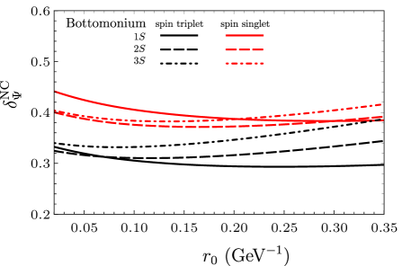
Figure 6: The non-Coulombic corrections $\delta_{\Psi}^{\rm NC}$ at finite $r_{0}$ for the bottomonium $1S$ (solid lines), $2S$ (dashed lines), and $3S$ (dot-dashed lines) states, for spin triplet (black) and spin singlet (red). The $r_{0}$ dependences are mild for the range 0.05 GeV${}^{-1}<r_{0}<$ 0.2 GeV^-1 that we consider.

State	$\Psi^{\rm LO}(0)$ (GeV3/2)	$E^{\rm LO}$ (GeV)	$\delta_{\Psi}^{\rm NC}|_{\bm{S}^{2}=2}$	$\delta_{\Psi}^{\rm NC}|_{\bm{S}^{2}=0}$	$\delta_{\Psi}^{\rm C1}$	$\delta_{\Psi}^{\rm C2}$	$\delta_{\Psi}^{\rm RS^{\prime}}$
$1S$	0.496	0.023	0.305	0.405	0.241	$-0.018$	0.016
$2S$	0.423	0.417	0.311	0.376	0.108	$-0.009$	0.013
$3S$	0.400	0.723	0.332	0.384	0.068	$-0.003$	0.012

Table 2: LO wavefunctions at the origin, LO binding energies and the relative corrections to the wavefunctions at the origin in the $\overline{\rm MS}$ scheme at scale $\Lambda=m$ for $1S$, $2S$, and $3S$ bottomonium states. $\delta_{\Psi}^{\rm NC}$ is the correction from the $1/m$ and $1/m^{2}$ potentials, $\delta_{\Psi}^{\rm C1}$ and $\delta_{\Psi}^{\rm C2}$ are Coulombic corrections at first and second order in QMPT, respectively, and $\delta_{\Psi}^{\rm RS^{\prime}}$ is the correction from the $\rm RS^{\prime}$ subtraction term. The $\delta_{\Psi}^{\rm NC}$, $\delta_{\Psi}^{\rm C1}$, $\delta_{\Psi}^{\rm C2}$, and $\delta_{\Psi}^{\rm RS^{\prime}}$ are dimensionless.

The results for the LO binding energies for the $1S$, $2S$ and $3S$ states in table 2 are roughly compatible with the mass differences between $\Upsilon(1S)$, $\Upsilon(2S)$, and $\Upsilon(3S)$ states. We see that the non-Coulombic corrections from $1/m$ and $1/m^{2}$ potentials, given by $\delta_{\Psi}^{\rm NC}$ in table 2, are large and positive for the $1S$, $2S$, and $3S$ states, although the relative sizes of the corrections are smaller than the case of charmonium $1S$ and $2S$ states. As it was in the case of charmonia, the order-$\alpha_{s}^{2}$ corrections to the SDCs in appendix C are large and negative at $\Lambda=m$, so that if we combine the pNRQCD expressions of the LDMEs with the SDCs, large cancellations will occur between the order-$\alpha_{s}^{2}$ corrections to the SDCs and the corrections to the wavefunctions at the origin. The contribution from the long-distance part of the $1/m$ potential, originating from the second term in the expression for the $1/m$ potential in eq. (100), amounts to about $+4\%$, $+2\%$, and $+2\%$ of the LO wavefunction at the origin for the $1S$, $2S$, and $3S$ states, respectively, which are less than half of the corresponding corrections to the charmonium wavefunctions at the origin. We note that while the Coulombic corrections at first order are positive, the Coulombic corrections at second order are small and negative, signaling good convergence of the Coulombic corrections. The corrections from the renormalon subtraction term $\delta_{\Psi}^{\rm RS^{\prime}}$ are small.

As it was in the case of charmonium, the LO wavefunctions at the origin in table 2 are larger than what we obtain if we neglect the long-distance nonperturbative part of the static potential. Neglecting the long-distance part of the static potential reduces the wavefunctions at the origin for the $2S$ and $3S$ states by more than factors of 3 and 6, respectively, while for the $1S$ state, the wavefunction at the origin reduces by a factor of about $1.5$. At the squared amplitude level, neglecting the long-distance part of the static potential can reduce the $2S$ bottomonium decay rates by almost an order of magnitude, and the $3S$ bottomonium decay rates by more than an order of magnitude. Hence, even for the bottomonium states, the nonperturbative long-distance part of the static potential is important, especially for the $2S$ and $3S$ states.

Now we compute the decay constants $f_{\Upsilon(nS)}$, $f_{\eta_{b}(nS)}$, and the electromagnetic decay rates of $\Upsilon(nS)$ and $\eta_{b}(nS)$ based on the bottomonium wavefunctions at the origin that we obtained. We use the same pNRQCD expressions for these quantities in eqs. (112), (117), and (120) that we used in the previous section for the charmonium states, except that we set $n_{f}=4$ in the SDCs, and use $e_{Q}=-1/3$ for bottom. We note that the correction terms in the pNRQCD expressions of the LDMEs in eqs. (10) and (13) that come from the gluonic correlators may not be valid for $1S$ bottomonium states, because the assumption $mv\gtrsim\Lambda_{\rm QCD}\gg mv^{2}$ may not hold for these states. Hence, when we make predictions for the bottomonium $1S$ states, we assume that eqs. (112), (117), and (120) are valid up to corrections of order $v^{2}$.

The numerical results for the decay constants $f_{\Upsilon(nS)}$ are

$$f_{\Upsilon(1S)} = 0.621{}^{+0.045}_{-0.000}{}^{+0.008}_{-0.006}\pm 0.033\pm 0.062\textrm{~{}GeV}=0.621{}^{+0.084}_{-0.070}\textrm{~{}GeV},$$ (123a)

$$f_{\Upsilon(2S)} = 0.447{}^{+0.002}_{-0.000}{}^{+0.003}_{-0.003}\pm 0.024\pm 0.013\textrm{~{}GeV}=0.447{}^{+0.028}_{-0.027}\textrm{~{}GeV},$$ (123b)

$$f_{\Upsilon(3S)} = 0.395{}^{+0.001}_{-0.000}{}^{+0.006}_{-0.000}\pm 0.021\pm 0.012\textrm{~{}GeV}=0.395{}^{+0.025}_{-0.024}\textrm{~{}GeV},$$ (123c)

where the first uncertainties come from varying $\mu_{R}$ between 2 GeV and 8 GeV, and the second uncertainties come from varying $r_{0}$ between 0.05 GeV^-1 and 0.2 GeV^-1. The third uncertainties take into account the neglect of the correction $-V_{p^{2}}^{(2)}(0)/(2m)$ to the wavefunctions at the origin, which we take to be $\pm 500\textrm{~{}MeV}/(2m)$ times the central value. For $f_{\Upsilon(1S)}$, the final uncertainty comes from the uncalculated order-$v^{2}$ corrections to the LDME, which we take to be 10% of the central value. This is based on the typical estimate $v^{2}\approx 0.1$ for bottomonium states. For $f_{\Upsilon(2S)}$ and $f_{\Upsilon(3S)}$, the final uncertainties come from the uncalculated corrections of order $v^{3}$, which we take to be 3% of the central value, based on the typical estimate $v^{2}\approx 0.1$. We add the uncertainties in quadrature.

Compared to the LO values $f_{\Upsilon(nS)}^{\rm LO}$, the central values in eq. (123) are $12$% larger for $\Upsilon(1S)$, $3\%$ smaller for $\Upsilon(2S)$, and $8\%$ smaller for $\Upsilon(3S)$. If we had ignored the corrections to the wavefunctions at the origin, the order-$\alpha_{s}$ correction would have been $-18$% of the central value, while the order-$\alpha_{s}^{2}$ correction would have been $-20$% of the central value, so that the perturbative corrections to two-loop accuracy would add up to $-38\%$ of the central value. Similarly to the case of charmonia, inclusion of the corrections to the wavefunctions at the origin reduces the sizes of the corrections considerably, significantly improving the convergence of the corrections.

The results for $f_{\Upsilon(1S)}$ and $f_{\Upsilon(2S)}$ that we obtain agree well within uncertainties with the lattice NRQCD determinations $f_{\Upsilon(1S)}=0.639(31)$ GeV and $f_{\Upsilon(2S)}=0.481(39)$ GeV from ref. Colquhoun:2014ica , where the SDCs and the LDMEs are both obtained in lattice regularization, avoiding the use of the $\overline{\rm MS}$ scheme. In order to compare with experimental measurements, we compute the leptonic decay rates of $\Upsilon(nS)$ from $f_{\Upsilon(nS)}$ by using eq. (82). We obtain

$$\Gamma(\Upsilon(1S)\to e^{+}e^{-}) = 1.11{}^{+0.32}_{-0.24}\textrm{~{}keV},$$ (124a)

$$\Gamma(\Upsilon(2S)\to e^{+}e^{-}) = 0.54{}^{+0.07}_{-0.06}\textrm{~{}keV},$$ (124b)

$$\Gamma(\Upsilon(3S)\to e^{+}e^{-}) = 0.41{}^{+0.05}_{-0.05}\textrm{~{}keV},$$ (124c)

where we used $\alpha=1/131$, which is computed at the scale of the $\Upsilon(nS)$ mass. These results agree within uncertainties with the experimental values $\Gamma(\Upsilon(1S)\to e^{+}e^{-})=1.340\pm 0.018$ keV, $\Gamma(\Upsilon(2S)\to e^{+}e^{-})=0.612\pm 0.011$ keV, and $\Gamma(\Upsilon(3S)\to e^{+}e^{-})=0.443\pm 0.008$ keV in ref. Tanabashi:2018oca . If we use the expressions for the decay rates expanded at the squared amplitude level, we obtain $\Gamma(\Upsilon(1S)\to e^{+}e^{-})=1.10{}^{+0.23}_{-0.16}$ keV, $\Gamma(\Upsilon(2S)\to e^{+}e^{-})=0.54\pm 0.06$ keV, and $\Gamma(\Upsilon(3S)\to e^{+}e^{-})=0.41\pm 0.05$ keV, which agree well with the results in eq. (124) within uncertainties.

We note that the result for $\Gamma(\Upsilon(1S)\to e^{+}e^{-})$ that we obtain also agrees well with the perturbative QCD prediction at third order in ref. Beneke:2014qea . However, the convergence of the perturbative expansion in the perturbative QCD calculation is poor; according to ref. Beneke:2014qea , the size of the corrections at first and second order, when combined, exceeds the leading-order result, while the third order correction is moderate. In contrast, in the calculation of the decay rate $\Gamma(\Upsilon(1S)\to e^{+}e^{-})$ in this work, the loop corrections to the SDCs and the corrections to the wavefunction at the origin combine to be $25$% of the leading order result at the squared amplitude level. It seems that the improvement of the convergence has mostly to do with the Coulombic corrections, because the non-Coulombic correction $\delta_{\Psi}^{\rm NC}$ does not change much from the result in table 2 when we neglect the long-distance, nonperturbative part of the LO potential given by the second term in eq. (91). Hence, the convergence of the perturbative QCD calculation may improve if the logarithms associated with the loop corrections to the static potential are resummed, as we have done in computing the Coulombic corrections.

The numerical results for the decay constants $f_{\eta_{b}(nS)}$ are

$$f_{\eta_{b}(1S)} = 0.691{}^{+0.117}_{-0.015}{}^{+0.010}_{-0.010}\pm 0.037\pm 0.069\textrm{~{}GeV}=0.691{}^{+0.141}_{-0.080}\textrm{~{}GeV},$$ (125a)

$$f_{\eta_{b}(2S)} = 0.471{}^{+0.006}_{-0.004}{}^{+0.005}_{-0.002}\pm 0.025\pm 0.014\textrm{~{}GeV}=0.471{}^{+0.030}_{-0.029}\textrm{~{}GeV},$$ (125b)

$$f_{\eta_{b}(3S)} = 0.403{}^{+0.000}_{-0.002}{}^{+0.004}_{-0.000}\pm 0.021\pm 0.012\textrm{~{}GeV}=0.403{}^{+0.026}_{-0.025}\textrm{~{}GeV},$$ (125c)

where the uncertainties are as in eq. (123). We neglect the small uncertainty from the scale dependence of the correlator ${\cal E}_{3}$. We add the uncertainties in quadrature. Compared to the LO results $f_{\eta_{b}(nS)}^{\rm LO}$, the central values in eq. (125) are $23$% larger for $\eta_{b}(1S)$, $1\%$ larger for $\eta_{b}(2S)$, and $7\%$ smaller for $\eta_{b}(3S)$. If we had ignored the corrections to the wavefunctions at the origin, the order-$\alpha_{s}$ correction would have been $-14$% of the central value, while the order-$\alpha_{s}^{2}$ correction would have been $-24$% of the central value, so that the perturbative corrections to two-loop accuracy would add up to $-38\%$ of the central value. Inclusion of the corrections to the wavefunctions at the origin reduces the sizes of the corrections considerably, especially for $\eta_{b}(2S)$ and $\eta_{b}(3S)$, greatly improving the convergence of the corrections.

The numerical results for the decay rates $\Gamma(\eta_{b}(nS)\to\gamma\gamma)$ are

$$\Gamma(\eta_{b}(1S)\to\gamma\gamma) = 0.433{}^{+0.142}_{-0.016}{}^{+0.013}_{-0.012}{}^{+0.047}_{-0.045}\pm 0.043\textrm{~{}keV}=0.433{}^{+0.165}_{-0.065}\textrm{~{}keV},$$ (126a)

$$\Gamma(\eta_{b}(2S)\to\gamma\gamma) = 0.194{}^{+0.003}_{-0.002}{}^{+0.004}_{-0.001}{}^{+0.021}_{-0.020}\pm 0.006\textrm{~{}keV}=0.194{}^{+0.022}_{-0.021}\textrm{~{}keV},$$ (126b)

$$\Gamma(\eta_{b}(3S)\to\gamma\gamma) = 0.141{}^{+0.000}_{-0.005}{}^{+0.003}_{-0.001}{}^{+0.015}_{-0.014}\pm 0.004\textrm{~{}keV}=0.141{}^{+0.016}_{-0.015}\textrm{~{}keV},$$ (126c)

where the uncertainties are as in $f_{\Upsilon(nS)}$. We add the uncertainties in quadrature. Compared to the LO calculation of the decay rates, the corrections from loop corrections to the SDCs and the corrections to the wavefunctions at the origin combine to be about 58%, 15%, and 3% for the $\eta_{b}(1S)$, $\eta_{b}(2S)$, and $\eta_{b}(3S)$ states, respectively. At the amplitude level, the corrections amount to about 26%, 7%, and 2% for the $\eta_{b}(1S)$, $\eta_{b}(2S)$, and $\eta_{b}(3S)$ states, respectively. If we had ignored the corrections to the wavefunctions at the origin, the order-$\alpha_{s}$ correction would have been $-11$%, and the order-$\alpha_{s}^{2}$ correction would have been $-26$% of the central value at the amplitude level, so that the loop corrections to two-loop accuracy would add up to $-38\%$ of the leading-order amplitude. By the inclusion of the corrections to the wavefunctions at the origin, the sizes of the corrections are reduced considerably for the $\eta_{b}(2S)$ and $\eta_{b}(3S)$ states, while the improvement is moderate for the $\eta_{b}(1S)$ state. If we use the expressions for the decay rates expanded at the squared amplitude level, we obtain $\Gamma(\eta_{b}(1S)\to\gamma\gamma)=0.422^{+0.155}_{-0.064}$ keV, $\Gamma(\eta_{b}(2S)\to\gamma\gamma)=0.196\pm 0.022$ keV, and $\Gamma(\eta_{b}(3S)\to\gamma\gamma)=0.142\pm 0.016$ keV, which agree well with the results in eq. (126).

6 Summary and discussion

In this paper, we have computed the wavefunctions at the origin of $S$-wave heavy quarkonia in the $\overline{\rm MS}$ renormalization scheme. We include the nonperturbative long-distance contributions to the potential, which are neglected in perturbative QCD calculations. We compute corrections to the wavefunctions at the origin at subleading orders in $1/m$ in position space, where the ultraviolet divergences are regulated by using finite-$r$ regularization. The position-space expressions for the corrections to the wavefunctions at the origin are given in section 3. The wavefunctions at the origin in finite-$r$ regularization is then converted to the $\overline{\rm MS}$ scheme by computing the scheme conversion in perturbative QCD. The result for the scheme conversion coefficient is given in section 4. We use the results for the wavefunctions at the origin to make first-principles based, model-independent predictions of decay constants and electromagnetic decay rates of $S$-wave charmonium and bottomonium states in section 5.

The predictions for the electromagnetic decay rates of $J/\psi$, $\psi(2S)$, $\eta_{c}$, and $\Upsilon(nS)$ states in this work agree with experimental measurements within uncertainties. The predictions for the $J/\psi$ and $\eta_{c}$ decay constants agree within uncertainties with lattice QCD calculations in ref. Hatton:2020qhk , which make use of relativistic charm quarks. The predictions for the $\Upsilon(1S)$ and $\Upsilon(2S)$ decay constants agree with the lattice NRQCD determinations in ref. Colquhoun:2014ica , where lattice regularization is used to compute both the short-distance coefficients and the NRQCD matrix elements.

The calculation of the wavefunctions at the origin in this work contains several improvements compared to existing model dependent methods. First of all, in this work, we include potentials at leading and subleading orders in $1/m$, which are determined by perturbative QCD at short distances, while their nonperturbative behaviors at long distances are fixed by lattice QCD. Secondly, the ultraviolet divergences that appear in corrections to the wavefunctions at the origin are properly renormalized in the $\overline{\rm MS}$ scheme, so that the wavefunctions at the origin that we obtain have the correct scale dependences that are expected from perturbative QCD. Finally, the ambiguity in the heavy quark pole mass is removed by the use of the modified renormalon subtracted mass, whose numerical values are accurately known. These improvements are generally not possible in potential-model calculations.

Because the wavefunctions at the origin that we have computed have the correct scale dependence that reproduce the anomalous dimensions of NRQCD LDMEs, the dependences on the NRQCD factorization scale cancel completely through two-loop order in the pNRQCD expressions for the decay constants and electromagnetic decay rates. Together with the order-by-order cancellation of the dependence on the QCD renormalization scale, this greatly reduces the uncertainty associated with scale dependences.

A novel feature of the calculation of the decay constants and decay rates in this work is that large cancellations occur between the corrections to the wavefunctions at the origin and the perturbative corrections to the short-distance coefficients. These cancellations substantially improve the convergence of the expansion in $\alpha_{s}$ and $v$. This may have important implications in understanding the appearance of large perturbative corrections in calculations of short-distance coefficients in the $\overline{\rm MS}$ scheme. A possible explanation of the cancellations is that, due to the confining nature of the nonperturbative potentials, including the long-distance contributions to the potentials in calculating the wavefunctions at the origin may have the effect of introducing an infrared cutoff, so that the renormalon ambiguities associated with the infrared contributions of loop corrections in perturbative QCD are resolved.

The pNRQCD expressions of the wavefunctions at the origin, as well as the decay constants and decay rates, depend on gluonic correlators, whose values are in general not well known. Especially, the correction from the velocity-dependent potential at zero distance, which is given by a gluonic correlator whose size is of order $\Lambda_{\rm QCD}$, is the largest source of uncertainties, with the exception of the bottomonium $1S$ states. Improved determinations of the gluonic correlators, which can in principle be done in lattice QCD, will be necessary in further reducing the uncertainties.

The calculation of the renormalization of the wavefunctions at the origin in this work is accurate to two-loop accuracy. In principle, the calculation in this work can be extended to three-loop accuracy, by computing the divergent corrections to the wavefunctions at the origin to second order in the quantum-mechanical perturbation theory, and computing the scheme conversion from finite-$r$ regularization to the $\overline{\rm MS}$ scheme to order-$\alpha_{s}^{3}$ accuracy. Such a calculation will make possible the inclusion of the long-distance nonperturbative contributions to the potentials of order $1/m^{2}$, because the second-order correction in the quantum-mechanical perturbation theory is necessary in extending the calculation of the unitary transformation between on-shell matching and Wilson-loop matching in section 4 to order-$1/m^{2}$ accuracy.

Finally, we note that the calculation in this paper may be extended to states with nonzero orbital angular momentum. This necessarily involves considering the orbital angular momentum dependent terms in the potential, as well as the angular dependence of the wavefunctions in dimensional regularization, which were not present in this work thanks to the rotational symmetry of the $S$-wave states. Such calculations will allow us to make accurate predictions of production and decay rates of $P$-wave heavy quarkonium states.

Appendix A Anomalous dimensions

In this appendix, we compute the anomalous dimensions of the NRQCD LDMEs that are given in eqs. (3) and (5). Although the results are available in refs. Bodwin:1994jh ; Czarnecki:1997vz ; Beneke:1997jm ; Czarnecki:2001zc ; Kniehl:2006qw , it can be useful to compute them through loop calculations in NRQCD, because such calculations can reveal the origins of the anomalous dimensions which are obscure in perturbative QCD calculations of SDCs.

The anomalous dimensions can be computed as perturbation series in $\alpha_{s}$ by replacing the quarkonium states in the definitions of the LDMEs by perturbative $Q\bar{Q}$ states, and computing loop corrections to the LDMEs, with the vertices coming from the operators in the NRQCD Lagrangian. The $Q$ and $\bar{Q}$ in the $Q\bar{Q}$ states are on shell, which have nonrelativistic 4-momenta $(E,\bm{q})$ and $(E,-\bm{q})$, respectively, where $E=\bm{q}^{2}/(2m)$. We work in Coulomb gauge, and use the NRQCD Feynman rules given in ref. Bodwin:1998mn . We use DR in $d=4-2\epsilon$ spacetime dimensions, where the anomalous dimensions are simply given by the coefficients of the $1/\epsilon$ poles that are associated with UV divergences.

The NRQCD loop integrals are evaluated in the following way. First, we integrate over the temporal components of the loop momenta, using contour integration. Then, we expand the integrand in powers of $1/m$, which is necessary in preserving the nonrelativistic power counting in DR. Finally, we integrate over the spatial components of the loop momenta, regulating the resulting divergences in DR. The anomalous dimension is given by the coefficients of the single UV poles, after differentiating and multiplying by $g_{s}=\sqrt{4\pi\alpha_{s}}$.

A.1 One-loop anomalous dimension at relative order $v^{2}$

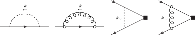
Figure 7: Feynman diagrams for one-loop corrections to the NRQCD LDMEs. Solid lines are heavy quarks and antiquarks, dashed lines are temporal gluons, and curly lines are transverse gluons. Open circles represent insertions of the $\bm{p}\cdot\bm{A}$ vertex, and filled squares represent the operator $\chi^{\dagger}\bm{\epsilon}\cdot\bm{\sigma}\psi$ for spin triplet, and $\chi^{\dagger}\psi$ for spin singlet.

We first consider the one-loop corrections to the NRQCD LDMEs $\langle 0|\chi^{\dagger}\bm{\epsilon}\cdot\bm{\sigma}\psi|Q\bar{Q}\rangle$ and $\langle 0|\chi^{\dagger}\psi|Q\bar{Q}\rangle$, which come from the Feynman diagrams in fig. 7. Because the one-loop integrals that we compute only involve single poles in $\epsilon$, we may set $\epsilon=0$ in the loop integrands without affecting the $1/\epsilon$ poles.

The one-loop heavy quark self energy from the first two diagrams in fig. 7 reads

$$\Sigma(E,\bm{q})=2\pi\alpha_{s}C_{F}\int_{\bm{k}}\frac{1}{\bm{k}^{2}}+\frac{4\pi\alpha_{s}C_{F}}{m^{2}}\int_{\bm{k}}\frac{\bm{q}^{2}-(\bm{q}\cdot\hat{\bm{k}})^{2}}{(2|\bm{k}|-i\varepsilon)[E-|\bm{k}|-(\bm{q}+\bm{k})^{2}/(2m)+i\varepsilon]},$$ (127)

where the first and second terms come from exchange of temporal and spatial gluons, respectively. The first term is scaleless power divergent, and therefore can be discarded. Since the second term already has a factor of $\bm{q}^{2}/m^{2}$, we can expand in powers of $1/m$ and keep only the leading contribution. To find the one-loop correction to the quark field renormalization factor $Z_{Q}^{\rm NRQCD}$, we differentiate $\Sigma(E,\bm{q})$ by $E$ and set $E=\bm{q}^{2}/(2m)$ to obtain

$$Z_{Q}^{\rm NRQCD}=1-\frac{2\pi\alpha_{s}C_{F}}{m^{2}}\int_{\bm{k}}\frac{\bm{q}^{2}-(\bm{q}\cdot\hat{\bm{k}})^{2}}{|\bm{k}|^{3}}=1-\frac{\alpha_{s}C_{F}}{3\pi}\frac{\bm{q}^{2}}{m^{2}}\frac{1}{\epsilon_{\rm UV}}+\cdots,$$ (128)

where we only keep the UV pole in the last equality. We use the subscript UV to make clear that the pole is associated with a UV divergence.

The vertex correction diagram from exchange of a temporal gluon gives

$$4\pi\alpha_{s}C_{F}m\int_{\bm{k}}\frac{1}{\bm{k}^{2}(\bm{k}^{2}+2\bm{q}\cdot\bm{k}-i\varepsilon)},$$ (129)

which does not have a UV divergence, and hence does not contribute to the anomalous dimension. The transverse-gluon exchange diagram gives

$$\frac{2\pi\alpha_{s}C_{F}}{m^{2}}\int_{\bm{k}}\frac{\bm{q}^{2}-(\bm{q}\cdot\hat{\bm{k}})^{2}}{A(\bm{k}^{2}-A^{2}-i\varepsilon)}-\frac{2\pi\alpha_{s}C_{F}}{m^{2}}\int_{\bm{k}}\frac{\bm{q}^{2}-(\bm{q}\cdot\hat{\bm{k}})^{2}}{(|\bm{k}|-i\varepsilon)(|\bm{k}|+A-i\varepsilon)(|\bm{k}|-A-i\varepsilon)},$$ (130)

where $A=(\bm{k}+\bm{q})^{2}/(2m)-\bm{q}^{2}/(2m)-i\varepsilon$. Here, the first term comes from the residue of the pole from the quark propagator, and the second term comes from the residue of the pole from the gluon propagator. Since eq. (130) already has a factor of $\bm{q}^{2}/m^{2}$, we can keep only the leading contribution in the $1/m$ expansion, which gives

$$\frac{2\pi\alpha_{s}C_{F}}{m^{2}}\int_{\bm{k}}\frac{\bm{q}^{2}-(\bm{q}\cdot\hat{\bm{k}})^{2}}{A(\bm{k}^{2}-i\varepsilon)}-\frac{2\pi\alpha_{s}C_{F}}{m^{2}}\int_{\bm{k}}\frac{\bm{q}^{2}-(\bm{q}\cdot\hat{\bm{k}})^{2}}{|\bm{k}|^{3}}=-\frac{\alpha_{s}C_{F}}{3\pi}\frac{\bm{q}^{2}}{m^{2}}\frac{1}{\epsilon_{\rm UV}}+\cdots,$$ (131)

where we only keep the UV pole. We note that the first term on the left-hand side does not have a UV divergence, and the UV pole comes only from the second term. It can be shown that if we replace the $\bm{p}\cdot\bm{A}$ vertices with $\bm{\sigma}\cdot\bm{B}$ vertices, the transverse-gluon exchange diagram does not produce logarithmic UV divergences.

Since the diagrams in fig. 7 give rise to logarithmic UV divergences at relative order $\alpha_{s}v^{2}$ already at leading power in the $1/m$ expansion, it is not necessary to consider vertices from higher dimensional operators in the NRQCD Lagrangian. We combine eqs. (128) and (131) to find the UV pole in the one-loop correction to the NRQCD LDME $\langle 0|\chi^{\dagger}\bm{\epsilon}\cdot\bm{\sigma}\psi|Q\bar{Q}\rangle$, which reads

$$\langle 0|\chi^{\dagger}\bm{\epsilon}\cdot\bm{\sigma}\psi|Q\bar{Q}\rangle|_{\textrm{one loop}} = -\frac{2\alpha_{s}C_{F}}{3\pi}\frac{\bm{q}^{2}}{m^{2}}\frac{1}{\epsilon_{\rm UV}}\langle 0|\chi^{\dagger}\bm{\epsilon}\cdot\bm{\sigma}\psi|Q\bar{Q}\rangle|_{\textrm{tree}}+\cdots$$ (132)

$$= -\frac{4\alpha_{s}C_{F}}{3\pi m^{2}}\frac{1}{2\epsilon_{\rm UV}}\langle 0|\chi^{\dagger}\bm{\epsilon}\cdot\bm{\sigma}(-\tfrac{i}{2}\overleftrightarrow{\bm{D}})^{2}\psi|Q\bar{Q}\rangle|_{\textrm{tree}}+\cdots,$$

where we used $\langle 0|\chi^{\dagger}\bm{\epsilon}\cdot\bm{\sigma}(-\tfrac{i}{2}\overleftrightarrow{\bm{D}})^{2}\psi|Q\bar{Q}\rangle=\bm{q}^{2}\langle 0|\chi^{\dagger}\bm{\epsilon}\cdot\bm{\sigma}\psi|Q\bar{Q}\rangle$ at tree level. This confirms the order-$\alpha_{s}v^{2}$ term of the anomalous dimension in eq. (3). Similarly, the UV pole in the one-loop correction to the LDME $\langle 0|\chi^{\dagger}\psi|Q\bar{Q}\rangle$ is

$$\langle 0|\chi^{\dagger}\psi|Q\bar{Q}\rangle|_{\textrm{one loop}}=-\frac{4\alpha_{s}C_{F}}{3\pi m^{2}}\frac{1}{2\epsilon_{\rm UV}}\langle 0|\chi^{\dagger}(-\tfrac{i}{2}\overleftrightarrow{\bm{D}})^{2}\psi|Q\bar{Q}\rangle|_{\textrm{tree}}+\cdots,$$ (133)

which confirms the order-$\alpha_{s}v^{2}$ term of the anomalous dimension in eq. (5).

Since the logarithmic UV divergences in the vertex correction diagrams come from the contribution from the gluon pole, there are no contributions to the anomalous dimension at relative order $\alpha_{s}v^{2}$ that comes from gluon exchanges between the quark and the antiquark when the virtual quark or the virtual antiquark is on shell. Hence, at one loop level, there is no contribution to the anomalous dimension that comes from exchanges of potentials between the $Q$ and $\bar{Q}$. This is consistent with the pNRQCD expressions of the LDMEs in eqs. (10) and (13), where the one-loop anomalous dimension comes from the gluonic correlator ${\cal E}_{3}$, and not from corrections to the wavefunctions at the origin.

A.2 Two-loop anomalous dimension at leading order in $v$

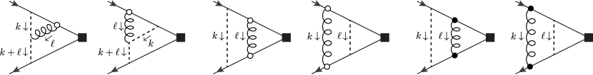
Figure 8: Feynman diagrams for two-loop corrections to the NRQCD LDMEs that produce logarithmic UV divergences. There are additional diagrams that can be obtained from charge conjugation, which we do not show here. Solid lines are heavy quarks and antiquarks, dashed lines are temporal gluons, and curly lines are transverse gluons. Open and filled circles represent insertions of the $\bm{p}\cdot\bm{A}$ vertex and the spin-dependent $\bm{\sigma}\cdot\bm{B}$ vertex, respectively. Filled squares represent the operator $\chi^{\dagger}\bm{\epsilon}\cdot\bm{\sigma}\psi$ for spin triplet, and $\chi^{\dagger}\psi$ for spin singlet.

Now let us consider the UV divergences in the two-loop corrections to the NRQCD LDMEs. Since we work at leading order in $v$, we can set the relative momentum $\bm{q}$ between the quark and antiquark to zero. The two-loop diagrams that contain logarithmic UV divergences are shown in fig. 8. We neglect diagrams that do not contain logarithmic UV divergences, most of which are scaleless power divergent, and hence vanish in DR. As we will see later, in the Coulomb gauge the diagrams only involve single poles in $\epsilon$, and hence, we can set $\epsilon=0$ in the numerators of loop integrands without affecting the $1/\epsilon$ poles. The non-Abelian diagrams yield

$$16\pi^{2}\alpha_{s}^{2}C_{A}C_{F}\int_{\bm{k}}\int_{\bm{\ell}}\frac{\bm{k}^{2}-(\bm{k}\cdot\hat{\bm{\ell}})^{2}}{\bm{\ell}^{2}\bm{k}^{2}(\bm{k}+\bm{\ell})^{4}}=\frac{\alpha_{s}^{2}C_{A}C_{F}}{8}\frac{1}{\epsilon_{\rm UV}}+\cdots,$$ (134)

where we only keep the UV pole. The spin-independent ladder diagrams yield

$$16\pi^{2}\alpha_{s}^{2}C_{F}^{2}\int_{\bm{k}}\int_{\bm{\ell}}\frac{\bm{k}^{2}-(\bm{k}\cdot\hat{\bm{\ell}})^{2}}{\bm{k}^{4}\bm{\ell}^{2}(\bm{k}+\bm{\ell})^{2}}=\frac{\alpha_{s}^{2}C_{F}^{2}}{8}\frac{1}{\epsilon_{\rm UV}}+\cdots,$$ (135)

where again we only keep the UV pole. The spin-dependent ladder diagrams give

$$4\pi^{2}\alpha_{s}^{2}C_{F}^{2}\int_{\bm{k}}\int_{\bm{\ell}}\left(\frac{\delta^{il}-\hat{\ell}^{i}\hat{\ell}^{l}}{\bm{k}^{4}\bm{\ell}^{2}(\bm{k}+\bm{\ell})^{2}}+\frac{\delta^{il}-\hat{\ell}^{i}\hat{\ell}^{l}}{\bm{k}^{2}\bm{\ell}^{4}(\bm{k}+\bm{\ell})^{2}}\right)\epsilon_{ijk}\ell_{j}\sigma_{k}\otimes\sigma_{n}\epsilon_{lmn}\ell_{m},$$ (136)

where we use the notation $\otimes$ to make clear that the Pauli matrix on the left acts on the quark line, while the one on the right acts on the antiquark line. We first integrate over $\bm{k}$, and average over the angles of $\bm{\ell}$ to obtain the following UV-divergent contribution from the spin-dependent ladder diagrams:

$$\pi^{2}\alpha_{s}^{2}C_{F}^{2}\int_{\bm{\ell}}\frac{1}{|\bm{\ell}|^{3+2\epsilon}}\frac{\sigma_{i}\otimes\sigma_{i}}{3}=\frac{\alpha_{s}^{2}C_{F}^{2}}{8}\frac{1}{\epsilon_{\rm UV}}\frac{\sigma_{i}\otimes\sigma_{i}}{3}+\cdots,$$ (137)

where again we keep only the UV pole. The spin-dependent factor $\sigma_{i}\otimes\sigma_{i}$ yields, for spin triplet,

$$\frac{1}{3}\sigma_{i}\bm{\epsilon}\cdot\bm{\sigma}\sigma_{i}=-\frac{1}{3}\bm{\epsilon}\cdot\bm{\sigma},$$ (138)

and for spin singlet,

$$\frac{1}{3}\sigma_{i}\sigma_{i}=1.$$ (139)

We collect the results in eqs. (134), (135), and (137) to obtain the logarithmic UV divergence in the two-loop correction to the LDME $\langle 0|\chi^{\dagger}\bm{\epsilon}\cdot\bm{\sigma}\psi|Q\bar{Q}\rangle$, which reads

$$\langle 0|\chi^{\dagger}\bm{\epsilon}\cdot\bm{\sigma}\psi|Q\bar{Q}\rangle|_{\textrm{two loop}}=\alpha_{s}^{2}C_{F}\left(\frac{C_{F}}{3}+\frac{C_{A}}{2}\right)\frac{1}{4\epsilon_{\rm UV}}\langle 0|\chi^{\dagger}\bm{\epsilon}\cdot\bm{\sigma}\psi|Q\bar{Q}\rangle|_{\textrm{tree}}+\cdots.$$ (140)

This reproduces the order-$\alpha_{s}^{2}$ term of the anomalous dimension in eq. (3). Similarly, the logarithmic UV divergence in the two-loop correction to the LDME $\langle 0|\chi^{\dagger}\psi|Q\bar{Q}\rangle$ is

$$\langle 0|\chi^{\dagger}\psi|Q\bar{Q}\rangle|_{\textrm{two loop}}=\alpha_{s}^{2}C_{F}\left(C_{F}+\frac{C_{A}}{2}\right)\frac{1}{4\epsilon_{\rm UV}}\langle 0|\chi^{\dagger}\psi|Q\bar{Q}\rangle|_{\textrm{tree}}+\cdots,$$ (141)

which agrees with the order-$\alpha_{s}^{2}$ term of the anomalous dimension in eq. (5).

We note that in the calculation of the two-loop diagrams in fig. 8, at least one of the integrations over the temporal components of the loop momenta must involve residues of the poles from the quark or antiquark propagators in order to produce logarithmic UV divergences. This is clear in the ladder diagrams, because the temporal-gluon propagator does not have a pole in the temporal components of loop momenta. For the non-Abelian diagrams, it can be shown that if we neglect the pole that comes from the transverse gluon propagator in the integration over $\ell_{0}$, we obtain the same UV pole as in eq. (134). This shows that the two-loop anomalous dimensions come solely from exchanges of potentials between the $Q$ and $\bar{Q}$. This is consistent with the pNRQCD expressions of the NRQCD LDMEs in eqs. (10) and (13), which imply that the two-loop anomalous dimension can only come from the wavefunctions at the origin.

Appendix B Potentials in perturbative QCD

In this appendix, we list the short-distance behaviors of the potentials, which are obtained from perturbative QCD. In perturbative QCD, the static potential is given through relative order $\alpha_{s}^{2}$ by Fischler:1977yf ; Schroder:1998vy

$$V^{(0)}(r)\big{|}_{\rm pert}=-\frac{\alpha_{s}(\mu)C_{F}}{r}\left[1+\sum_{n=1}^{2}\left(\frac{\alpha_{s}(\mu)}{4\pi}\right)^{n}a_{n}(r;\mu)\right]+O(\alpha_{s}^{3}),$$ (142)

where $\alpha_{s}=\alpha_{s}(\mu)$ is the $\overline{\rm MS}$-renormalized QCD coupling constant at scale $\mu$, and the functions $a_{n}(r;\mu)$ are defined by

$$a_{1}(r;\mu) = \frac{31C_{A}-20T_{F}n_{f}}{9}+2\beta_{0}\log(\mu e^{\gamma_{\rm E}}r),$$ (143a)

$$a_{2}(r;\mu) = \frac{400n_{f}^{2}T_{F}^{2}}{81}-C_{F}T_{F}n_{f}\left(\frac{55}{3}-16\,\xi(3)\right)$$ (143b)

$$+C_{A}^{2}\left(\frac{4343}{162}+\frac{16\pi^{2}-\pi^{4}}{4}+\frac{22\,\xi(3)}{3}\right)-C_{A}T_{F}n_{f}\left(\frac{1798}{81}+\frac{56\,\xi(3)}{3}\right)$$

$$+\frac{\pi^{2}}{3}\beta_{0}^{2}+\left(4\bar{a}_{1}\beta_{0}+2\beta_{1}\right)\log(\mu e^{\gamma_{\rm E}}r)+4\beta_{0}^{2}\log^{2}(\mu e^{\gamma_{\rm E}}r),$$

with $\beta_{0}=\frac{11}{3}C_{A}-\frac{4}{3}T_{F}n_{f}$, $\beta_{1}=\frac{34}{3}C_{A}^{2}-\frac{20}{3}C_{A}T_{F}n_{f}-4C_{F}T_{F}n_{f}$, $T_{F}=\frac{1}{2}$, $\gamma_{\rm E}$ is the Euler-Mascheroni constant, $n_{f}$ is the number of light quark flavors, and $\bar{a}_{1}=a_{1}(r=e^{-\gamma_{\rm E}}/\mu;\mu)$. We note that the dependence on $\mu$ cancels order by order in eq. (142). The corrections at relative order $\alpha_{s}^{3}$ have been computed in refs. Brambilla:1999qa ; Kniehl:1999ud ; Smirnov:2008pn ; Anzai:2009tm ; Smirnov:2009fh , and the position-space expression can be found in ref. Pineda:2011dg .

The forms of the $1/m$ and $1/m^{2}$ potentials generally depend on the matching scheme in which the potentials are determined. In on-shell matching, where we match on-shell $S$-matrix elements in NRQCD and pNRQCD in momentum space, we obtain Gupta:1982kp ; Pantaleone:1987qh ; Titard:1993nn ; Manohar:2000hj ; Kniehl:2001ju ; Kniehl:2002br ; Beneke:1999qg ; Beneke:2013jia

$$V^{(1)}(r)\big{|}_{\rm pert}^{\rm OS} = \frac{\alpha_{s}^{2}C_{F}(\tfrac{1}{2}C_{F}-C_{A})}{2r^{2}}+O(\alpha_{s}^{3}),$$ (144a)

$$V_{r}^{(2)}(r)\big{|}_{\rm pert}^{\rm OS} = 0+O(\alpha_{s}^{2}),$$ (144b)

$$V_{p^{2}}^{(2)}(r)\big{|}_{\rm pert}^{\rm OS} = -\frac{\alpha_{s}C_{F}}{r}+O(\alpha_{s}^{2}),$$ (144c)

$$V_{S^{2}}^{(2)}(r)\big{|}_{\rm pert}^{\rm OS} = \frac{4\pi\alpha_{s}C_{F}}{3}\delta^{(3)}(\bm{r})+O(\alpha_{s}^{2}).$$ (144d)

We use the superscript OS to denote the on-shell matching scheme.

In Wilson-loop matching, the potentials are given in terms of the rectangular Wilson loop $W_{r\times T}$ with spatial size $r$ and time extension $T$, with insertions of the gluon fields. The nonperturbative expressions for the $1/m$ potential and the velocity-dependent potential in Wilson loop matching are given by Brambilla:2000gk ; Pineda:2000sz

$$V^{(1)}(r)\big{|}^{\rm WL} = -\lim_{T\to\infty}\int_{0}^{T}dt\,t\left(\langle\!\langle g_{s}\bm{E}_{1}^{i}(t)g_{s}\bm{E}_{1}^{j}(0)\rangle\!\rangle-\langle\!\langle g_{s}\bm{E}_{1}^{i}(t)\rangle\!\rangle\langle\!\langle g_{s}\bm{E}_{1}^{j}(0)\rangle\!\rangle\right),$$ (145a)

$$V_{p^{2}}^{(2)}(r)\big{|}^{\rm WL} = i\hat{\bm{r}}^{i}\hat{\bm{r}}^{j}\lim_{T\to\infty}\int_{0}^{T}dt\,t^{2}\left(\langle\!\langle g_{s}\bm{E}_{1}^{i}(t)g_{s}\bm{E}_{1}^{j}(0)\rangle\!\rangle-\langle\!\langle g_{s}\bm{E}_{1}^{i}(t)\rangle\!\rangle\langle\!\langle g_{s}\bm{E}_{1}^{j}(0)\rangle\!\rangle\right)$$ (145b)

$$+i\hat{\bm{r}}^{i}\hat{\bm{r}}^{j}\lim_{T\to\infty}\int_{0}^{T}dt\,t^{2}\left(\langle\!\langle g_{s}\bm{E}_{1}^{i}(t)g_{s}\bm{E}_{2}^{j}(0)\rangle\!\rangle-\langle\!\langle g_{s}\bm{E}_{1}^{i}(t)\rangle\!\rangle\langle\!\langle g_{s}\bm{E}_{2}^{j}(0)\rangle\!\rangle\right),\quad\quad$$

where $\langle\!\langle\cdots\rangle\!\rangle\equiv\langle\cdots W_{r\times T}\rangle/\langle W_{r\times T}\rangle$, $\hat{\bm{r}}=\bm{r}/|\bm{r}|$, the angular brackets $\langle\cdots\rangle$ stand for the average over the Yang-Mills action, and $g_{s}\bm{E}_{1}(t)$ ($g_{s}\bm{E}_{2}(t)$) are insertions of the chromoelectric field $\bm{E}^{i}=G^{i0}$ at time $t$ on the quark (antiquark) line of the Wilson loop, with $G^{\mu\nu}$ being the gluon field-strength tensor. The superscript WL denotes that the potential is obtained in Wilson loop matching. The complicated expressions for $V^{(2)}_{r}(r)$ and $V_{S^{2}}^{(2)}(r)$ can be found in ref. Pineda:2000sz . The short-distance behavior of the potentials in Wilson loop matching can be obtained by computing the nonperturbative definitions in perturbative QCD Peset:2015vvi . We list the results at leading nonvanishing orders in $\alpha_{s}$:

$$V^{(1)}(r)\big{|}_{\rm pert}^{\rm WL} = -\frac{\alpha_{s}^{2}C_{F}C_{A}}{2r^{2}}+O(\alpha_{s}^{3}),$$ (146a)

$$V^{(2)}_{r}(r)\big{|}_{\rm pert}^{\rm WL} = \pi\alpha_{s}C_{F}\delta^{(3)}(\bm{r})+O(\alpha_{s}^{2}),$$ (146b)

$$V_{p^{2}}^{(2)}(r)\big{|}_{\rm pert}^{\rm WL} = -\frac{\alpha_{s}C_{F}}{r}+O(\alpha_{s}^{2}),$$ (146c)

$$V_{S^{2}}^{(2)}(r)\big{|}_{\rm pert}^{\rm WL} = \frac{4\pi\alpha_{s}C_{F}}{3}\delta^{(3)}(\bm{r})+O(\alpha_{s}^{2}).$$ (146d)

The potentials from on-shell matching in eq. (144) and the potentials from Wilson loop matching in eq. (146) are related by unitary transformations, as described in section 4.4.

Appendix C Short-distance coefficients

In this appendix, we list the NRQCD factorization formulas and SDCs for the decay constants and decay rates that we consider in sec. 5. The NRQCD factorization formula for the decay constant $f_{V}$ of a vector quarkonium $V$ reads

$$f_{V}=\frac{\sqrt{2m_{V}}}{m_{V}}\left(c_{v}\langle 0|\chi^{\dagger}\bm{\epsilon}\cdot\bm{\sigma}\psi|V\rangle+\frac{d_{v}}{m^{2}}\langle 0|\chi^{\dagger}\bm{\epsilon}\cdot\bm{\sigma}(-\tfrac{i}{2}\overleftrightarrow{\bm{D}})^{2}\psi|V\rangle+O(v^{3})\right),$$ (147)

where $m_{V}$ is the mass of the quarkonium $V$, and the SDCs $c_{v}$ and $d_{v}$ are given in the $\overline{\rm MS}$ scheme by Barbieri:1975ki ; Celmaster:1978yz ; Czarnecki:1997vz ; Beneke:1997jm ; Keung:1982jb ; Luke:1997ys ; Bodwin:2008vp

$$c_{v} = 1-\frac{2\alpha_{s}(m)C_{F}}{\pi}+\left(\frac{\alpha_{s}(m)}{\pi}\right)^{2}\bigg{[}C_{F}^{2}c_{v,A}+C_{F}C_{A}c_{v,NA}$$ (148a)

$$\hskip 137.77734pt+C_{F}T_{F}n_{f}c_{v,L}+C_{F}T_{F}c_{v,H}\bigg{]}+O(\alpha_{s}^{3}),$$

$$d_{v} = -\frac{1}{6}+\frac{2\alpha_{s}C_{F}}{9\pi}\left(1-3\log\frac{m^{2}}{\Lambda^{2}}\right)+O(\alpha_{s}^{2}),$$ (148b)

and

$$c_{v,A} = \frac{23}{8}-\frac{\zeta(3)}{2}+\pi^{2}\log 2-\frac{76\pi^{2}}{36}+\frac{\pi^{2}}{6}\log\frac{m^{2}}{\Lambda^{2}},$$ (149a)

$$c_{v,NA} = -\frac{151}{72}-\frac{13}{4}\zeta(3)-\frac{5\pi^{2}}{6}\log 2+\frac{89\pi^{2}}{144}+\frac{\pi^{2}}{4}\log\frac{m^{2}}{\Lambda^{2}},$$ (149b)

$$c_{v,L} = \frac{11}{18},$$ (149c)

$$c_{v,H} = -\frac{2\pi^{2}}{9}+\frac{22}{9}.$$ (149d)

Here, $\Lambda$ is the scale at which the NRQCD LDMEs are renormalized. The expression for $c_{v}$ in eq. (148a) is valid when $\alpha_{s}$ is evaluated in the $\overline{\rm MS}$ scheme at the scale $m$. Since the QCD renormalization scale dependence cancels order by order in $c_{v}$, eq. (148a) is still valid if we replace $\alpha_{s}(m)$ by $\alpha_{s}(\mu_{R})$ and add $-\frac{2\alpha_{s}C_{F}}{\pi}\times\frac{\alpha_{s}\beta_{0}}{4\pi}\log(\mu_{R}^{2}/m^{2})$, which compensates for the running of $\alpha_{s}$. We note that the order-$\alpha_{s}^{3}$ correction to $c_{v}$ have been obtained in ref. Marquard:2014pea .

The NRQCD factorization formula for the decay constant $f_{P}$ of a pseudoscalar quarkonium $P$ reads

$$f_{P}=\frac{\sqrt{2m_{P}}}{m_{P}}\left(c_{p}\langle 0|\chi^{\dagger}\psi|P\rangle+\frac{d_{p}}{m^{2}}\langle 0|\chi^{\dagger}(-\tfrac{i}{2}\overleftrightarrow{\bm{D}})^{2}\psi|P\rangle+O(v^{3})\right),$$ (150)

where $m_{P}$ is the mass of the quarkonium $P$, and $c_{p}$ and $d_{p}$ read, in the $\overline{\rm MS}$ scheme Braaten:1995ej ; Kniehl:2006qw ; Wang:2017bgv ,

$$c_{p} = 1-\frac{3\alpha_{s}(m)C_{F}}{2\pi}+\left(\frac{\alpha_{s}(m)}{\pi}\right)^{2}\bigg{[}C_{F}^{2}c_{p,A}+C_{F}C_{A}c_{p,NA}$$ (151a)

$$\hskip 86.11084pt+C_{F}T_{F}n_{f}c_{p,L}+C_{F}T_{F}c_{p,H}+C_{F}T_{F}X_{\rm sing}^{(p)}\bigg{]}+O(\alpha_{s}^{3}),$$

$$d_{p} = -\frac{1}{2}+O(\alpha_{s}),$$ (151b)

and

$$c_{p,A} = \frac{29}{16}-\frac{79}{8}\zeta(2)+6\zeta(2)\log 2+\frac{9}{2}\zeta(3)+3\zeta(2)\log\frac{m^{2}}{\Lambda^{2}},$$ (152a)

$$c_{p,NA} = -\frac{17}{48}+\frac{17}{8}\zeta(2)-6\zeta(2)\log 2-3\zeta(3)+\frac{3}{2}\zeta(2)\log\frac{m^{2}}{\Lambda^{2}},$$ (152b)

$$c_{p,L} = \frac{1}{12},$$ (152c)

$$c_{p,H} = \frac{43}{12}-2\zeta(2),$$ (152d)

$$X_{\rm sing}^{(p)} = \frac{5}{4}\zeta(2)+3\zeta(2)\log 2-\frac{21}{8}\zeta(3)+\frac{3}{4}i\pi\zeta(2).$$ (152e)

Again, $\Lambda$ is the scale at which the NRQCD LDMEs are renormalized. The imaginary part in $X_{\rm sing}^{(p)}$ arises from the process $Q\bar{Q}\to gg\to Q\bar{Q}$, where the gluons are on shell Kniehl:2006qw .

To the best of the author’s knowledge, the order-$\alpha_{s}$ correction to $d_{p}$ has not been computed yet. Since the QCD renormalization scale dependence cancels order by order in $c_{p}$, eq. (151a) is still valid if we replace $\alpha_{s}(m)$ by $\alpha_{s}(\mu_{R})$ and add $-\frac{3\alpha_{s}C_{F}}{2\pi}\times\frac{\alpha_{s}\beta_{0}}{4\pi}\log(\mu_{R}^{2}/m^{2})$, which compensates for the running of $\alpha_{s}$.

Finally, the two-photon decay rate of a pseudoscalar quarkonium $P$ is given by

$$\Gamma(P\to\gamma\gamma)=\frac{8\pi\alpha^{2}e_{Q}^{4}}{m_{P}^{2}}\left|c_{\gamma\gamma}\langle 0|\chi^{\dagger}\psi|P\rangle+\frac{d_{\gamma\gamma}}{m^{2}}\langle 0|\chi^{\dagger}(-\tfrac{i}{2}\overleftrightarrow{\bm{D}})^{2}\psi|P\rangle+O(v^{3})\right|^{2},$$ (153)

where the SDCs $c_{\gamma\gamma}$ and $d_{\gamma\gamma}$ are given in the $\overline{\rm MS}$ scheme by Harris:1957zza ; Barbieri:1979be ; Hagiwara:1980nv ; Keung:1982jb ; Bodwin:1994jh ; Czarnecki:2001zc ; Feng:2015uha ; Jia:2011ah ; Guo:2011tz

$$c_{\gamma\gamma} = 1-\frac{\alpha_{s}(m)C_{F}}{\pi}\left(\frac{\pi^{2}}{8}-\frac{5}{2}\right)$$ (154a)

$$+\left(\frac{\alpha_{s}(m)}{\pi}\right)^{2}\bigg{[}\frac{\pi^{2}}{2}C_{F}\left(C_{F}+\frac{C_{A}}{2}\right)\log\left(\frac{m^{2}}{\Lambda^{2}}\right)+f^{(2)}_{\rm reg}+f^{(2)}_{\rm lbl}\bigg{]}+O(\alpha_{s}^{3}),$$

$$d_{\gamma\gamma} = -\frac{1}{6}+\frac{\alpha_{s}C_{F}}{\pi}\left(-\frac{7}{36}-\frac{4}{3}\log 2-\frac{\pi^{2}}{16}-\frac{2}{3}\log\frac{m^{2}}{\Lambda^{2}}\right)+O(\alpha_{s}^{2}).$$ (154b)

Here, $\Lambda$ is the scale at which the NRQCD LDMEs are renormalized. The constants $f^{(2)}_{\rm reg}$ and $f^{(2)}_{\rm lbl}$ have been determined numerically in ref. Feng:2015uha , which read

$$f^{(2)}_{\rm reg} = -21.10789797(4)\,C_{F}^{2}-4.79298000(3)\,C_{F}C_{A}+0.223672013(2)\,C_{F}T_{F}n_{H}$$ (155a)

$$-\left(\frac{13}{144}\pi^{2}+\frac{2}{3}\log(2)+\frac{7}{24}\zeta(3)-\frac{41}{36}\right)C_{F}T_{F}n_{f},$$

$$f^{(2)}_{\rm lbl} = \left[0.73128459+i\pi\left(\frac{\pi^{2}}{9}-\frac{5}{3}\right)\right]C_{F}T_{F}\sum_{q}\left(\frac{e_{q}}{e_{Q}}\right)^{2}$$ (155b)

$$+\big{(}0.64696557+2.07357556\,i\big{)}\,C_{F}T_{F}n_{H},$$

where $n_{H}=1$, $e_{q}$ is the fractional charge of the light quark with flavor $q$, and the sum runs over $n_{f}$ light quark flavors. The term $f^{(2)}_{\rm lbl}$ in $c_{\gamma\gamma}$ originates from the process where the $Q\bar{Q}$ decays into $gg$, which then decays into $\gamma\gamma$ via a quark loop Feng:2015uha . The imaginary parts in $f^{(2)}_{\rm lbl}$ arise from the region of loop momenta where the intermediate particles are on shell. Since the QCD renormalization scale dependence cancels order by order in $c_{\gamma\gamma}$, eq. (154a) is still valid if we replace $\alpha_{s}(m)$ by $\alpha_{s}(\mu_{R})$ and add $-\frac{\alpha_{s}C_{F}}{\pi}\left(\frac{\pi^{2}}{8}-\frac{5}{2}\right)\times\frac{\alpha_{s}\beta_{0}}{4\pi}\log(\mu_{R}^{2}/m^{2})$.

Appendix D Wavefunctions at the origin in perturbative QCD

If we ignore the nonperturbative long-distance behavior of the static potential, so that $V_{\rm LO}(r)=-\alpha_{s}C_{F}/r$, the Schrödinger equation can be solved exactly, and the $S$-wave contribution to the Green’s function in position space is known analytically:

$$G^{S}(\bm{r}^{\prime},\bm{r};E) = -\frac{\alpha_{s}C_{F}m^{2}}{4\pi}\Gamma(-\lambda)\exp\left({-\frac{1}{2\lambda}\alpha_{s}C_{F}m(r_{<}+r_{>})}\right)$$ (156)

$$\times{}_{1}F_{1}(1-\lambda;2;\alpha_{s}C_{F}mr_{<}/\lambda)\,U(1-\lambda;2;\alpha_{s}C_{F}mr_{>}/\lambda),$$

where $r_{<}={\rm min}(|\bm{r}|,|\bm{r}^{\prime}|)$, $r_{>}={\rm max}(|\bm{r}|,|\bm{r}^{\prime}|)$, $\lambda=\alpha_{s}C_{F}/\sqrt{-4E/m}$, and

$${}_{1}F_{1}(a;b;z) = \sum_{k=0}^{\infty}\frac{(a)_{k}}{(b)_{k}}\frac{z^{k}}{k!},$$ (157a)

$$U(a;b;z) = \frac{1}{\Gamma(a)}\int_{0}^{\infty}dt\,e^{-zt}t^{a-1}(1+t)^{b-a-1}.$$ (157b)

This result can be obtained by solving the differential equation in eq. (102) analytically. The bound states can be identified from the poles of $\Gamma(-\lambda)$, which are located at $\lambda=n$ with principal quantum numbers $n=1,2,3,\ldots$. The reduced Green’s functions can also be obtained analytically from eq. (156). This makes possible analytical calculations of the corrections to the $S$-wave wavefunctions at the origin. Such a calculation has been done in the context of heavy quark pair production near threshold in perturbative QCD in refs. Hoang:1998xf ; Melnikov:1998ug ; Penin:1998kx ; Hoang:1999zc ; Melnikov:1998pr ; Yakovlev:1998ke ; Beneke:1999qg ; Nagano:1999nw ; Penin:1998mx ; Penin:2004ay . We use the known results in perturbative QCD to check the numerical procedure used in this paper for computing the divergent corrections to the wavefunctions at the origin that originate from the $1/m$ and $1/m^{2}$ potentials.

The explicit analytical expressions for the two-loop non-Coulombic corrections to the wavefunctions at the origin from the $1/m$ and $1/m^{2}$ potentials can be found in ref. Penin:1998kx for the spin-triplet state. Rather than comparing the wavefunctions at the origin, which depends on the renormalization scheme, it is simpler to compare the corrections to the decay constant $f_{V}$, which is scale and scheme independent. At leading order in $\alpha_{s}$ and $v$, $f_{V}$ for the spin-triplet $nS$ state is given in perturbative QCD by

$$f_{V}^{\rm LO}\big{|}_{\textrm{pert}}=\sqrt{\frac{2N_{c}}{m}}|\Psi_{n}^{\rm LO}(0)|,$$ (158)

where $|\Psi_{n}^{\rm LO}(0)|^{2}=(\alpha_{s}C_{F}m)^{3}/(8\pi n^{3})$. The corrections to the wavefunctions at the origin coming from the $1/m$ and $1/m^{2}$ potentials are given in ref. Penin:1998kx by

$$|\Psi_{n}(0)| = |\Psi_{n}^{\rm LO}(0)|\times\bigg{\{}1-\frac{1}{2}\alpha_{s}^{2}C_{F}\bigg{[}\frac{15C_{F}}{8n^{2}}+\left(\frac{2}{3}C_{F}+C_{A}\right)$$ (159)

$$\hskip 107.63855pt\times\left(H_{n-1}-\frac{1}{n}-\log\left(\frac{2\mu_{f}n}{\alpha_{s}C_{F}m}\right)\right)\bigg{]}+\cdots\bigg{\}},$$

where $\mu_{f}$ is a factorization scale, and the ellipsis represent the Coulombic corrections that we neglect. The wavefunctions at the origin in ref. Penin:1998kx are renormalized in a scheme that is different from the $\overline{\rm MS}$ scheme that we use in this paper, so it is not possible to compare eq. (159) directly with the results in this paper. This scheme dependence cancels in the decay constant against the scheme dependence in the hard matching coefficient given by eq. (2) in ref. Penin:1998kx , which is obtained from the direct matching procedure Hoang:1997ui . Since the non-Coulombic corrections are proportional to $\alpha_{s}^{2}C_{F}^{2}$ and $\alpha_{s}^{2}C_{F}C_{A}$, we only need to keep the contributions that are proportional to $C_{F}^{2}$ and $C_{F}C_{A}$ in the loop corrections to the hard matching coefficient. By combining the corrections to the wavefunctions at the origin and the hard matching coefficient, we obtain the two-loop non-Coulombic correction given by

$$\delta_{f}^{\rm NC} = -\frac{1}{2}\alpha_{s}^{2}C_{F}\bigg{[}\frac{15C_{F}}{8n^{2}}+\left(\frac{2}{3}C_{F}+C_{A}\right)\left(H_{n-1}-\frac{1}{n}-\log\left(\frac{2\mu_{f}n}{\alpha_{s}C_{F}m}\right)\right)\bigg{]}$$ (160)

$$+\left(\frac{\alpha_{s}}{\pi}\right)^{2}\bigg{[}\bigg{(}\frac{23}{8}-\frac{\zeta(3)}{2}+\frac{2\pi^{2}}{3}\log 2-\frac{35\pi^{2}}{36}+\frac{\pi^{2}}{6}\log\frac{m^{2}}{\mu_{f}^{2}}\bigg{)}C_{F}^{2}$$

$$\hskip 43.05542pt+\bigg{(}-\frac{151}{72}-\frac{13}{4}\zeta(3)-\frac{4\pi^{2}}{3}\log 2+\frac{179\pi^{2}}{144}+\frac{\pi^{2}}{4}\log\frac{m^{2}}{\mu_{f}^{2}}\bigg{)}C_{F}C_{A}\bigg{]},\quad$$

where the last two lines correspond to the $C_{F}^{2}$ and the $C_{F}C_{A}$ terms of the two-loop corrections to the hard matching coefficients in ref. Penin:1998kx . The $\mu_{f}$ dependence cancels exactly between the non-Coulombic corrections to the wavefunctions at the origin and the two-loop corrections to the hard matching coefficient. Note that the last two lines of eq. (160) differ from the $C_{F}^{2}$ and the $C_{F}C_{A}$ terms of the two-loop corrections to the SDC $c_{v}$ in eq. (148a). This reflects the difference between the renormalization scheme used in ref. Penin:1998kx and the $\overline{\rm MS}$ scheme used in this work. This analytical result can be compared with the numerical calculation in this paper, which is given by

$$\delta_{f}^{\rm NC} = \delta_{\Psi}^{\rm NC}\big{|}_{\rm pert}+\left(\frac{\alpha_{s}}{\pi}\right)^{2}\left(C_{F}^{2}c_{v,A}+C_{F}C_{A}c_{v,NA}\right),$$ (161)

where $\delta_{\Psi}^{\rm NC}\big{|}_{\rm pert}$ is equal to eq. (110a), except that we set $V_{\rm LO}(r)=-\alpha_{s}C_{F}/r$, $V_{p^{2}}^{(2)}(0)=0$, and we take the perturbative $1/m$ and $1/m^{2}$ potentials in eq. (144). The dependence on $\Lambda$ cancels exactly in eq. (161) between $\delta_{\Psi}^{\rm NC}\big{|}_{\rm pert}$ and the SDCs $c_{v,A}$ and $c_{v,NA}$.

Figure 9: Comparison of numerical calculations and analytical results for the non-Coulombic corrections $\delta_{f}^{\rm NC}$ to the decay constant of vector quarkonium in perturbative QCD for various values of $\alpha_{s}$. Numerical results are shown as filled circles ($1S$), open circles ($2S$), and open squares ($3S$). The analytical results are shown as solid line ($1S$), dashed line ($2S$), and dot-dashed line ($3S$).

We compare the numerical calculation in eq. (161) with the analytical result in eq. (160) for $n=1$, 2, and 3 in fig. 9. We set $m=4.743$ GeV, $r_{0}=10^{-4}$ GeV^-1, and vary $\alpha_{s}$ between $0.15$ and $0.3$. The agreement between the numerical calculations and the analytical results is better than 1%. This agreement demonstrates the validity of the numerical calculation in this work.

References

- (1) N. Brambilla et al., Heavy Quarkonium: Progress, Puzzles, and Opportunities, Eur. Phys. J. C 71 (2011) 1534 [1010.5827].
- (2) N. Brambilla et al., QCD and Strongly Coupled Gauge Theories: Challenges and Perspectives, Eur. Phys. J. C 74 (2014) 2981 [1404.3723].
- (3) W. E. Caswell and G. P. Lepage, Effective Lagrangians for Bound State Problems in QED, QCD, and Other Field Theories, Phys. Lett. 167B (1986) 437.
- (4) G. T. Bodwin, E. Braaten and G. P. Lepage, Rigorous QCD analysis of inclusive annihilation and production of heavy quarkonium, Phys. Rev. D51 (1995) 1125 [hep-ph/9407339].
- (5) E. Eichten, K. Gottfried, T. Kinoshita, K. Lane and T.-M. Yan, Charmonium: The Model, Phys. Rev. D 17 (1978) 3090.
- (6) W. Buchmüller and S. Tye, Quarkonia and Quantum Chromodynamics, Phys. Rev. D 24 (1981) 132.
- (7) E. J. Eichten and C. Quigg, Quarkonium wave functions at the origin, Phys. Rev. D 52 (1995) 1726 [hep-ph/9503356].
- (8) G. T. Bodwin, H. S. Chung, D. Kang, J. Lee and C. Yu, Improved determination of color-singlet nonrelativistic QCD matrix elements for S-wave charmonium, Phys. Rev. D 77 (2008) 094017 [0710.0994].
- (9) H. S. Chung, J. Lee and C. Yu, NRQCD matrix elements for S-wave bottomonia and Gamma[eta_b(nS) -> gamma gamma] with relativistic corrections, Phys. Lett. B 697 (2011) 48 [1011.1554].
- (10) A. Czarnecki and K. Melnikov, Two loop QCD corrections to the heavy quark pair production cross-section in e+ e- annihilation near the threshold, Phys. Rev. Lett. 80 (1998) 2531 [hep-ph/9712222].
- (11) M. Beneke, A. Signer and V. A. Smirnov, Two loop correction to the leptonic decay of quarkonium, Phys. Rev. Lett. 80 (1998) 2535 [hep-ph/9712302].
- (12) A. Czarnecki and K. Melnikov, Charmonium decays: J / psi —> e+ e- and eta(c) —> gamma gamma, Phys. Lett. B 519 (2001) 212 [hep-ph/0109054].
- (13) B. Kniehl, A. Onishchenko, J. Piclum and M. Steinhauser, Two-loop matching coefficients for heavy quark currents, Phys. Lett. B 638 (2006) 209 [hep-ph/0604072].
- (14) G. T. Bodwin, S. Kim and D. Sinclair, Matrix elements for the decays of S and P wave quarkonium: An exploratory study, Nucl. Phys. B Proc. Suppl. 34 (1994) 434.
- (15) G. T. Bodwin, D. Sinclair and S. Kim, Quarkonium decay matrix elements from quenched lattice QCD, Phys. Rev. Lett. 77 (1996) 2376 [hep-lat/9605023].
- (16) G. T. Bodwin, D. Sinclair and S. Kim, Lattice calculation of quarkonium decay matrix elements, Int. J. Mod. Phys. A 12 (1997) 4019 [hep-ph/9609371].
- (17) G. T. Bodwin, D. Sinclair and S. Kim, Bottomonium decay matrix elements from lattice QCD with two light quarks, Phys. Rev. D 65 (2002) 054504 [hep-lat/0107011].
- (18) G. T. Bodwin, J. Lee and D. Sinclair, Spin correlations and velocity-scaling in NRQCD matrix elements, AIP Conf. Proc. 756 (2005) 384 [hep-lat/0412006].
- (19) G. T. Bodwin, J. Lee and D. Sinclair, Spin correlations and velocity-scaling in color-octet NRQCD matrix elements, Phys. Rev. D 72 (2005) 014009 [hep-lat/0503032].
- (20) A. Pineda and J. Soto, Effective field theory for ultrasoft momenta in NRQCD and NRQED, Nucl. Phys. B Proc. Suppl. 64 (1998) 428 [hep-ph/9707481].
- (21) N. Brambilla, A. Pineda, J. Soto and A. Vairo, Potential NRQCD: An Effective theory for heavy quarkonium, Nucl. Phys. B566 (2000) 275 [hep-ph/9907240].
- (22) N. Brambilla, A. Pineda, J. Soto and A. Vairo, Effective Field Theories for Heavy Quarkonium, Rev. Mod. Phys. 77 (2005) 1423 [hep-ph/0410047].
- (23) N. Brambilla, A. Pineda, J. Soto and A. Vairo, The QCD potential at O(1/m), Phys. Rev. D 63 (2001) 014023 [hep-ph/0002250].
- (24) A. Pineda and A. Vairo, The QCD potential at O (1 / : Complete spin dependent and spin independent result, Phys. Rev. D 63 (2001) 054007 [hep-ph/0009145].
- (25) A. Hoang and T. Teubner, Top quark pair production at threshold: Complete next-to-next-to-leading order relativistic corrections, Phys. Rev. D 58 (1998) 114023 [hep-ph/9801397].
- (26) K. Melnikov and A. Yelkhovsky, Top quark production at threshold with O(alpha-s**2) accuracy, Nucl. Phys. B 528 (1998) 59 [hep-ph/9802379].
- (27) K. Melnikov and A. Yelkhovsky, The b quark low scale running mass from Upsilon sum rules, Phys. Rev. D 59 (1999) 114009 [hep-ph/9805270].
- (28) A. Penin and A. Pivovarov, Bottom quark pole mass and |V(cb)| matrix element from R(e+ e- —> b anti-b) and Gamma(sl)(b —> cl neutrino(l)) in the next to next-to-leading order, Nucl. Phys. B 549 (1999) 217 [hep-ph/9807421].
- (29) O. I. Yakovlev, Top quark production near threshold: NNLO QCD correction, Phys. Lett. B 457 (1999) 170 [hep-ph/9808463].
- (30) M. Beneke, A. Signer and V. A. Smirnov, Top quark production near threshold and the top quark mass, Phys. Lett. B 454 (1999) 137 [hep-ph/9903260].
- (31) T. Nagano, A. Ota and Y. Sumino, O(alpha(s)**2) corrections to e+ e- —> t anti-t total and differential cross-sections near threshold, Phys. Rev. D 60 (1999) 114014 [hep-ph/9903498].
- (32) A. Hoang and T. Teubner, Top quark pair production close to threshold: Top mass, width and momentum distribution, Phys. Rev. D 60 (1999) 114027 [hep-ph/9904468].
- (33) A. Penin and A. Pivovarov, Analytical results for e+ e- —> t anti-t and gamma gamma —> t anti-t observables near the threshold up to the next-to-next-to leading order of NRQCD, Phys. Atom. Nucl. 64 (2001) 275 [hep-ph/9904278].
- (34) A. Hoang et al., Top - anti-top pair production close to threshold: Synopsis of recent NNLO results, Eur. Phys. J. direct 2 (2000) 3 [hep-ph/0001286].
- (35) A. Penin, A. Pineda, V. A. Smirnov and M. Steinhauser, Spin dependence of heavy quarkonium production and annihilation rates: Complete next-to-next-to-leading logarithmic result, Nucl. Phys. B 699 (2004) 183 [hep-ph/0406175].
- (36) A. Pineda and J. Soto, Matching at one loop for the four quark operators in NRQCD, Phys. Rev. D 58 (1998) 114011 [hep-ph/9802365].
- (37) A. Pineda and J. Soto, Potential NRQED: The Positronium case, Phys. Rev. D 59 (1999) 016005 [hep-ph/9805424].
- (38) N. Brambilla, A. Pineda, J. Soto and A. Vairo, The Infrared behavior of the static potential in perturbative QCD, Phys. Rev. D 60 (1999) 091502 [hep-ph/9903355].
- (39) N. Brambilla, D. Eiras, A. Pineda, J. Soto and A. Vairo, Inclusive decays of heavy quarkonium to light particles, Phys. Rev. D 67 (2003) 034018 [hep-ph/0208019].
- (40) N. Brambilla, H. S. Chung, D. Müller and A. Vairo, Decay and electromagnetic production of strongly coupled quarkonia in pNRQCD, JHEP 04 (2020) 095 [2002.07462].
- (41) A. V. Manohar, The HQET / NRQCD Lagrangian to order alpha / m-3, Phys. Rev. D 56 (1997) 230 [hep-ph/9701294].
- (42) N. Brambilla, D. Eiras, A. Pineda, J. Soto and A. Vairo, New predictions for inclusive heavy quarkonium P wave decays, Phys. Rev. Lett. 88 (2002) 012003 [hep-ph/0109130].
- (43) K. G. Wilson, Confinement of Quarks, Phys. Rev. D 10 (1974) 2445.
- (44) L. Susskind, Coarse Grained Quantum Chromodynamics, in Ecole d’Ete de Physique Theorique - Weak and Electromagnetic Interactions at High Energy, pp. 207–308, 1, 1976.
- (45) L. S. Brown and W. I. Weisberger, Remarks on the Static Potential in Quantum Chromodynamics, Phys. Rev. D 20 (1979) 3239.
- (46) A. Pineda, Is there a linear potential at short distances?, Nucl. Phys. B Proc. Suppl. 133 (2004) 190 [hep-ph/0310135].
- (47) A. Bazavov, N. Brambilla, I. Tormo, Xavier Garcia, P. Petreczky, J. Soto and A. Vairo, Determination of from the QCD static energy: An update, Phys. Rev. D 90 (2014) 074038 [1407.8437].
- (48) Y. Koma, M. Koma and H. Wittig, Relativistic corrections to the static potential at O(1/m) and O(1/m**2), PoS LATTICE2007 (2007) 111 [0711.2322].
- (49) Y. Koma and M. Koma, Heavy quarkonium spectroscopy in pNRQCD with lattice QCD input, PoS LATTICE2012 (2012) 140 [1211.6795].
- (50) B. A. Kniehl, A. A. Penin, M. Steinhauser and V. A. Smirnov, NonAbelian alpha**3(s) / (m(q)r**2) heavy quark anti-quark potential, Phys. Rev. D 65 (2002) 091503 [hep-ph/0106135].
- (51) B. A. Kniehl, A. A. Penin, V. A. Smirnov and M. Steinhauser, Potential NRQCD and heavy quarkonium spectrum at next-to-next-to-next-to-leading order, Nucl. Phys. B 635 (2002) 357 [hep-ph/0203166].
- (52) C. Peset, A. Pineda and M. Stahlhofen, Potential NRQCD for unequal masses and the Bc spectrum at N3LO, JHEP 05 (2016) 017 [1511.08210].
- (53) Y. Kiyo, A. Pineda and A. Signer, New determination of inclusive electromagnetic decay ratios of heavy quarkonium from QCD, Nucl. Phys. B 841 (2010) 231 [1006.2685].
- (54) M. Beneke, Y. Kiyo and K. Schuller, Third-order correction to top-quark pair production near threshold I. Effective theory set-up and matching coefficients, 1312.4791.
- (55) A. Pineda, Review of Heavy Quarkonium at weak coupling, Prog. Part. Nucl. Phys. 67 (2012) 735 [1111.0165].
- (56) E. Braaten and Y.-Q. Chen, Dimensional regularization in quarkonium calculations, Phys. Rev. D 55 (1997) 2693 [hep-ph/9610401].
- (57) W. Fischler, Quark - anti-Quark Potential in QCD, Nucl. Phys. B 129 (1977) 157.
- (58) Y. Schroder, The Static potential in QCD to two loops, Phys. Lett. B 447 (1999) 321 [hep-ph/9812205].
- (59) A. Hoang, Perturbative O (alpha-s**2) corrections to the hadronic cross-section near heavy quark - anti-quark thresholds in e+ e- annihilation, Phys. Rev. D 56 (1997) 5851 [hep-ph/9704325].
- (60) S. J. Brodsky and G. Lepage, Exclusive Processes in Quantum Chromodynamics, Adv. Ser. Direct. High Energy Phys. 5 (1989) 93.
- (61) V. Chernyak and A. Zhitnitsky, Asymptotic Behavior of Exclusive Processes in QCD, Phys. Rept. 112 (1984) 173.
- (62) Y. Jia and D. Yang, Refactorizing NRQCD short-distance coefficients in exclusive quarkonium production, Nucl. Phys. B 814 (2009) 217 [0812.1965].
- (63) H. S. Chung, J.-H. Ee, D. Kang, U.-R. Kim, J. Lee and X.-P. Wang, Pseudoscalar Quarkonium+gamma Production at NLL+NLO accuracy, JHEP 10 (2019) 162 [1906.03275].
- (64) C. Davies, C. McNeile, E. Follana, G. Lepage, H. Na and J. Shigemitsu, Update: Precision decay constant from full lattice QCD using very fine lattices, Phys. Rev. D 82 (2010) 114504 [1008.4018].
- (65) HPQCD collaboration, Charmonium properties from lattice QCD + QED: hyperfine splitting, leptonic width, charm quark mass and , 2005.01845.
- (66) M. Beneke, Renormalons, Phys. Rept. 317 (1999) 1 [hep-ph/9807443].
- (67) A. Pineda, Determination of the bottom quark mass from the Upsilon(1S) system, JHEP 06 (2001) 022 [hep-ph/0105008].
- (68) C. Peset, A. Pineda and J. Segovia, The charm/bottom quark mass from heavy quarkonium at N3LO, JHEP 09 (2018) 167 [1806.05197].
- (69) M. Beneke, A Quark mass definition adequate for threshold problems, Phys. Lett. B 434 (1998) 115 [hep-ph/9804241].
- (70) TUMQCD collaboration, Relations between Heavy-light Meson and Quark Masses, Phys. Rev. D 97 (2018) 034503 [1712.04983].
- (71) K. Chetyrkin, J. H. Kuhn and M. Steinhauser, RunDec: A Mathematica package for running and decoupling of the strong coupling and quark masses, Comput. Phys. Commun. 133 (2000) 43 [hep-ph/0004189].
- (72) F. Herren and M. Steinhauser, Version 3 of RunDec and CRunDec, Comput. Phys. Commun. 224 (2018) 333 [1703.03751].
- (73) TXL, T(X)L collaboration, Static potentials and glueball masses from QCD simulations with Wilson sea quarks, Phys. Rev. D 62 (2000) 054503 [hep-lat/0003012].
- (74) G. S. Bali, QCD forces and heavy quark bound states, Phys. Rept. 343 (2001) 1 [hep-ph/0001312].
- (75) A. Laschka, N. Kaiser and W. Weise, Quark-antiquark potential to order 1/m and heavy quark masses, Phys. Rev. D 83 (2011) 094002 [1102.0945].
- (76) A. Laschka, N. Kaiser and W. Weise, Charmonium Potentials: Matching Perturbative and Lattice QCD, Phys. Lett. B 715 (2012) 190 [1205.3390].
- (77) G. Perez-Nadal and J. Soto, Effective string theory constraints on the long distance behavior of the subleading potentials, Phys. Rev. D 79 (2009) 114002 [0811.2762].
- (78) M. J. Strassler and M. E. Peskin, The Heavy top quark threshold: QCD and the Higgs, Phys. Rev. D 43 (1991) 1500.
- (79) Particle Data Group collaboration, Review of Particle Physics, Phys. Rev. D 98 (2018) 030001.
- (80) CLEO collaboration, Observation of eta-prime(c) production in gamma gamma fusion at CLEO, Phys. Rev. Lett. 92 (2004) 142001 [hep-ex/0312058].
- (81) Belle collaboration, Measurement of eta_c(1S), eta_c(2S) and non-resonant eta’ pi+ pi- production via two-photon collisions, Phys. Rev. D 98 (2018) 072001 [1805.03044].
- (82) B. Colquhoun, R. Dowdall, C. Davies, K. Hornbostel and G. Lepage, and Leptonic Widths, and from full lattice QCD, Phys. Rev. D 91 (2015) 074514 [1408.5768].
- (83) M. Beneke, Y. Kiyo, P. Marquard, A. Penin, J. Piclum, D. Seidel et al., Leptonic decay of the (1) meson at third order in QCD, Phys. Rev. Lett. 112 (2014) 151801 [1401.3005].
- (84) G. T. Bodwin and Y.-Q. Chen, Renormalon ambiguities in NRQCD operator matrix elements, Phys. Rev. D 60 (1999) 054008 [hep-ph/9807492].
- (85) B. A. Kniehl and A. A. Penin, Ultrasoft effects in heavy quarkonium physics, Nucl. Phys. B 563 (1999) 200 [hep-ph/9907489].
- (86) A. V. Smirnov, V. A. Smirnov and M. Steinhauser, Fermionic contributions to the three-loop static potential, Phys. Lett. B 668 (2008) 293 [0809.1927].
- (87) C. Anzai, Y. Kiyo and Y. Sumino, Static QCD potential at three-loop order, Phys. Rev. Lett. 104 (2010) 112003 [0911.4335].
- (88) A. V. Smirnov, V. A. Smirnov and M. Steinhauser, Three-loop static potential, Phys. Rev. Lett. 104 (2010) 112002 [0911.4742].
- (89) S. N. Gupta, S. F. Radford and W. W. Repko, Quarkonium Spectra and Quantum Chromodynamics, Phys. Rev. D 26 (1982) 3305.
- (90) J. T. Pantaleone and S. Tye, The Hyperfine Splitting of States in Heavy Quarkonia, Phys. Rev. D 37 (1988) 3337.
- (91) S. Titard and F. Yndurain, Rigorous QCD evaluation of spectrum and ground state properties of heavy q anti-q systems: With a precision determination of m(b) M(eta(b)), Phys. Rev. D 49 (1994) 6007 [hep-ph/9310236].
- (92) A. V. Manohar and I. W. Stewart, The QCD heavy quark potential to order v**2: One loop matching conditions, Phys. Rev. D 62 (2000) 074015 [hep-ph/0003032].
- (93) R. Barbieri, R. Gatto, R. Kogerler and Z. Kunszt, Meson hyperfine splittings and leptonic decays, Phys. Lett. B 57 (1975) 455.
- (94) W. Celmaster, Lepton Width Suppression in Vector Mesons, Phys. Rev. D 19 (1979) 1517.
- (95) W.-Y. Keung and I. Muzinich, Beyond the Static Limit for Quarkonium Decays, Phys. Rev. D 27 (1983) 1518.
- (96) M. E. Luke and M. J. Savage, Power counting in dimensionally regularized NRQCD, Phys. Rev. D 57 (1998) 413 [hep-ph/9707313].
- (97) G. T. Bodwin, H. S. Chung, J. Lee and C. Yu, Order-alpha(s) corrections to the quarkonium electromagnetic current at all orders in the heavy-quark velocity, Phys. Rev. D 79 (2009) 014007 [0807.2634].
- (98) P. Marquard, J. H. Piclum, D. Seidel and M. Steinhauser, Three-loop matching of the vector current, Phys. Rev. D 89 (2014) 034027 [1401.3004].
- (99) E. Braaten and S. Fleming, QCD radiative corrections to the leptonic decay rate of the B(c) meson, Phys. Rev. D 52 (1995) 181 [hep-ph/9501296].
- (100) W. Wang, J. Xu, D. Yang and S. Zhao, Relativistic corrections to light-cone distribution amplitudes of S-wave Bc mesons and heavy quarkonia, JHEP 12 (2017) 012 [1706.06241].
- (101) I. Harris and L. M. Brown, Radiative Corrections to Pair Annihilation, Phys. Rev. 105 (1957) 1656.
- (102) R. Barbieri, E. d’Emilio, G. Curci and E. Remiddi, Strong Radiative Corrections to Annihilations of Quarkonia in QCD, Nucl. Phys. B 154 (1979) 535.
- (103) K. Hagiwara, C. Kim and T. Yoshino, Hadronic Decay Rate of Ground State Paraquarkonia in Quantum Chromodynamics, Nucl. Phys. B 177 (1981) 461.
- (104) F. Feng, Y. Jia and W.-L. Sang, Can Nonrelativistic QCD Explain the Transition Form Factor Data?, Phys. Rev. Lett. 115 (2015) 222001 [1505.02665].
- (105) Y. Jia, X.-T. Yang, W.-L. Sang and J. Xu, correction to pseudoscalar quarkonium decay to two photons, JHEP 06 (2011) 097 [1104.1418].
- (106) H.-K. Guo, Y.-Q. Ma and K.-T. Chao, Corrections to Hadronic and Electromagnetic Decays of Heavy Quarkonium, Phys. Rev. D 83 (2011) 114038 [1104.3138].