Power fluctuations in a finite-time quantum Carnot engine

Abstract

Stability is an important property of small thermal machines with fluctuating power output. We here consider a finite-time quantum Carnot engine based on a degenerate multilevel system and study the influence of its finite Hilbert space structure on its stability. We optimize in particular its relative work fluctuations with respect to level degeneracy and level number. We find that its optimal performance may surpass those of nondegenerate two-level engines or harmonic oscillator motors. Our results show how to realize high-performance, high-stability cyclic quantum heat engines.

The Carnot engine is one of the most emblematic examples of a thermal machine. Since its introduction in 1824, it has become a representative model for all heat engines. The Carnot cycle simply consists of two isothermal (expansion and compression) steps and of two adiabatic (expansion and compression) processes cen01 . In its ideal reversible limit of infinite cycle duration, the Carnot motor is the most efficient heat engine. The corresponding Carnot efficiency, $\eta_{\text{C}}=1-T_{c}/T_{h}$, where $T_{c,h}$ are the respective temperatures of the cold and hot heat baths, is regarded as the first formulation of the second law of thermodynamics cen01 . The first experimental realization of a Carnot engine using a colloidal particle in an optical harmonic trap has been reported lately mar15 . In addition, the finite-time properties of the Carnot cycle have been well investigated theoretically both in the classical cur75 ; and77 ; gut78 ; rub79 ; sal81 ; ond83 ; esp10 ; cav17 and in the quantum gev92 ; gev92a ; wu06 ; qua07 ; abe11 ; wan12 ; all13 ; dan20 ; abi20 regimes. Strong emphasis has been put on the optimization of the performance of the engine for finite cycle durations, in particular on its average power output at the expense of its efficiency.

For classical microscopic heat engines, like the one implemented in the experiment of Ref. mar15 , thermal fluctuations are no longer negligible as is the case for macroscopic motors sei12 . As a result, key performance measures, such as efficiency ver14 ; ver14a ; pol15 ; man19 and power hol14 ; hol17 ; pie18 ; hol18 , are stochastic variables. In that context, attention has recently been drawn to power fluctuations as a limiting factor for the practical usefulness of thermal machines: heat engines should indeed ideally have high efficiency, large power output but small power fluctuations hol14 ; hol17 ; pie18 ; hol18 . A new figure of merit, the constancy, defined as the product of the variance of the power and time, has been introduced to characterize the stability of heat engines hol14 ; hol17 ; pie18 ; hol18 . While a strict trade-off between efficiency, power and constancy has been established for steady-state heat engines, implying that power fluctuations diverge at maximum efficiency and finite power pie18 , they may remain finite for quasistatic cyclic thermal machines hol18 . On the other hand, quantum motors are not only dominated by thermal fluctuations but also by quantum fluctuations.

In this paper, we investigate the generic features of the power fluctuations in a finite-time quantum Carnot engine in the quasistatic limit. We specifically study the interplay between power fluctuations, the finite dimensionality of the Hilbert space of the working medium and the degree of degeneracy of its levels. Degenerate finite level structures commonly appear in atomic foo05 , molecular bro13 and condensed-matter physics cha00 . An understanding of their influence on the stability of quantum heat engines is therefore essential for future experimental realizations of thermal devices in these systems baz03 . An important illustration of the effect of the finiteness of quantum systems on thermodynamic fluctuations is provided by the Schottky anomaly blu06 : the corresponding increase of the heat capacity at low temperatures does not occur in infinite dimensional systems like the harmonic oscillator, in which the energy is not bounded; it is, furthermore, strongly affected by level degeneracy and level number eva06 . We mention, however, that our results are not directly related to the Schottky anomaly.

In the following, we compute the inverse coefficient of variation for work, defined as the ratio of the mean work and its standard deviation eve98 , for a quasistatic quantum Carnot engine whose working medium is described by a homogeneous Hamiltonian of degree $-2$, ${\cal H}(b\bm{r})=b^{-2}{\cal H}(\bm{r})$. Such Hamiltonians characterize a large class of single-particle, many-body and nonlinear systems that exhibit equidistant spectra gri10 ; jar13 ; cam13 ; def14 ; bea16 . We obtain a general formula that only depends on the heat capacity and on the entropy variation during the hot isotherm. We use this expression to maximize the inverse coefficient of variation for work, with respect to the degree of degeneracy and the number of levels of the system, in order to attain optimal cyclic quantum engines that operate close to the Carnot efficiency with large power output and small power fluctuations. We illustrate our results by analyzing (i) a two-level system with arbitrary degeneracy, (ii) a nondegenerate system with arbitrary level number, and (iii) a three-level system with generic degree of degeneracy. In all cases the optimal inverse coefficient of variation for work may be numerically determined by solving a transcendental equation.

Finite-time quantum Carnot cycle. We consider a general quantum system with time-dependent Hamiltonian, $H_{t}=\omega_{t}{\cal H}$, as the working fluid of a finite-time quantum Carnot engine, with driving parameter $\omega_{t}$. The quantum Carnot cycle consists of the following four steps gev92 ; gev92a ; wu06 ; qua07 ; abe11 ; wan12 ; all13 ; dan20 ; abi20 : (1) hot isothermal expansion from $\omega_{1}$ to $\omega_{2}$, at temperature $T_{h}$ in time $\tau_{1}$, during which work $W_{1}$ is produced by the system and heat $Q_{h}$ is absorbed; (2) adiabatic expansion from $\omega_{2}$ to $\omega_{3}$, in time $\tau_{2}$, during which work $W_{2}$ is performed and the entropy remains constant. The system is here decoupled from the baths and its Hamiltonian commutes with itself at all times, $\left[H_{t},H_{t^{\prime}}\right]=0$. As a result, nonadiabatic transitions do not occur for all driving times $\tau_{2}$; (3) cold isothermal compression from $\omega_{3}$ to $\omega_{4}$, at temperature $T_{c}$ in time $\tau_{3}$, during which work $W_{3}$ is done on the system and heat $Q_{c}$ is released; (4) adiabatic compression from $\omega_{4}$ to $\omega_{1}$, in time $\tau_{4}$, during which work $W_{4}$ is unitarily performed on the system. The total cycle time is $\tau=\sum_{i}\tau_{i}$. Work and heat are taken positive when added to the system.

In order to evaluate the finite-time performance of the quantum Carnot engine, we will determine the mean and the variance of the stochastic work output $w$. The average total work, $W=\langle w\rangle=\sum_{i}W_{i}$, directly follows from the combination of the first and second law cen01 ,

$$W=-Q_{h}-Q_{c}=(T_{c}-T_{h})\Delta S,$$ (1)

where $\Delta S$ denotes the entropy change during the hot isotherm. Meanwhile, the total work fluctuations are characterized by the probability distribution $P(w)$,

$$P(w)=\langle\delta(w-\sum_{i}w_{i})\rangle,$$ (2)

where the average is taken over the joint probability distribution given by the convolution of the work densities of the four branches of the cycle, $P(w_{1},w_{2},w_{3},w_{4})=P_{1}(w_{1})\star P_{2}(w_{2})\star P_{3}(w_{3})\star P_{4}(w_{4})$ hol18 . The two isotherms (1) and (3) are assumed to be slower than the (fast) relaxation induced by the baths. The system thus remains in a thermal state and the two finite-time processes are quasistatic. In this case, the work distributions are sharp (with no fluctuations) and work is deterministic sup ,

$$P_{1,3}(w_{1,3})=\delta\left(w_{1,3}-W_{1,3}\right).$$ (3)

On the other hand, since no heat is exchanged during the two unitary adiabats (2) and (4), the corresponding work distributions can be obtained via the usual two-point-measurement scheme by projectively measuring the energy at the beginning and at the end of each step tal07 . Without level transitions, we obtain for process (2),

$$P_{2}(w_{2})=\sum_{n}\delta\left[w_{2}-(E_{3}^{n}-E_{2}^{n})\right]p^{n}_{2},$$ (4)

where $E_{2}^{n}$ and $E_{3}^{n}$ denote the respective eigenvalues of the Hamiltonians $H_{2}=H_{\tau_{1}}$ and $H_{3}=H_{\tau_{1}+\tau_{2}}$. The initial thermal distribution reads $p_{2}^{n}=\exp(-\beta_{h}E^{n}_{2})/z_{2}$ with inverse hot temperature $\beta_{h}$ and partition function $z_{2}$. We have similarly for transformation (4),

$$P_{4}(w_{4})=\sum_{m}\delta[w_{4}-(E_{1}^{m}-E_{4}^{m})]p^{m}_{4},$$ (5)

with $p_{4}^{m}=\exp(-\beta_{c}E^{m}_{4})/z_{4}$. In order to ensure that the system is in a thermal state at the end of each adiabat, and thus at the beginning of each isotherm, we adjust the adiabatic driving such that $\omega_{3}/\omega_{2}=\omega_{4}/\omega_{1}={\beta_{h}}/{\beta_{c}}$ dan20 . The whole Carnot cycle is hence quasistatic.

Combining the contributions of all the four branches of the cycle, we find the work output distribution,

$$P(w)=\langle\delta\left[w-\left(W-\widetilde{\Delta H_{2}}-\widetilde{\Delta H_{4}}\right)\right]\rangle,$$ (6)

where $W$ is given by Eq. (1). We have furthermore defined the (stochastic) difference $\widetilde{\Delta H_{i}}=\langle\Delta H_{i}\rangle-\Delta H_{i}$ and used the cycle condition $\sum_{i}\langle\Delta H_{i}\rangle$ = 0. The average in Eq. (6) may be computed using the Boltzmann distributions at the beginning of each adiabat sup .

Coefficient of variation for work. In statistics, the Fano factor (the ratio of the variance $\sigma^{2}$ and the mean) and the coefficient of variation (the ratio of the standard deviation $\sigma$ and the mean) are two measures of the dispersion of a probability distribution eve98 . For heat engines, the Fano factor for work, $\sigma_{w}^{2}/W$, is equal to the quotient of the constancy $\sigma^{2}_{P}\tau$ and the average power $P=W/\tau$ (defined over one cycle time) hol18 , while the corresponding coefficient of variation for work describes the relative work fluctuations. All the moments of the total work can be evaluated from Eq. (6) by integration $\langle w^{n}\rangle=\int dw~{}P(w)w^{n}$. The variance then reads sup ,

$$\sigma^{2}_{w}=\left(T_{c}-T_{h}\right)^{2}\left[C(\beta_{h},\omega_{2})+C(\beta_{c},\omega_{4})\right],$$ (7)

where we have introduced the heat capacity of the system, $C(\beta_{j},\omega_{i})=d\langle H_{i}\rangle/dT_{j}$, at the beginning of each adiabat sup . We accordingly obtain the Fano factor,

$$\frac{\sigma^{2}_{w}}{|W|}=\frac{\left(T_{h}-T_{c}\right)[C(\beta_{h},\omega_{2})+C(\beta_{c},\omega_{4})]}{\Delta S},$$ (8)

and the corresponding coefficient of variation,

$$\frac{\sigma_{w}}{|W|}=\frac{\sqrt{C(\beta_{h},\omega_{2})+C(\beta_{c},\omega_{4})}}{\Delta S}.$$ (9)

Equations (8) and (9) describe similar physics. However, in contrast to the Fano factor (8), the coefficient of variation (9) has the advantage that (i) it is a dimensionless quantity that (ii) depends solely on the heat capacities of the system (since the entropy variation can be written as an integral of the heat capacities sup ). We shall therefore focus on that quantity in the following.

A finite-time quantum Carnot engine with large work output and small work output fluctuations is characterized by a large inverse coefficient of variation $|W|/{\sigma_{w}}$. We will thus next optimize the inverse of Eq. (9) with respect to the degree of degeneracy and with respect to the number of levels of the working medium.

Degenerate two-level system. We begin by considering a degenerate qubit with Hamiltonian $H_{t}=\omega_{t}g_{1}\ket{1}\bra{1},$ where $g_{0}$ and $g_{1}$ are the respective degeneracies of the ground $\ket{0}$ and excited $\ket{1}$ states. The partition function at inverse temperature $\beta$ and frequency $\omega$ is $Z_{2}=g_{0}+g_{1}\exp(-\beta\omega)$ blu06 . The heat capacity then follows as,

$$C_{2}(\beta,\omega)=\frac{\gamma(\beta\omega)^{2}}{\left(e^{\beta\omega/2}+\gamma e^{-\beta\omega/2}\right)^{2}},$$ (10)

with the degeneracy ratio $\gamma=g_{1}/g_{0}$. The entropy difference during the hot isotherm further reads,

$$\Delta S_{2}=\frac{\beta_{c}\omega_{4}}{\gamma^{-1}e^{\beta_{c}\omega_{4}}+1}-\frac{\beta_{h}\omega_{2}}{\gamma^{-1}e^{\beta_{h}\omega_{2}}+1}+\ln\left[\frac{1+\gamma e^{-\beta_{h}\omega_{2}}}{1+\gamma e^{-\beta_{c}\omega_{4}}}\right].$$ (11)

The average of the work output (1) (blue), its variance (7) (red), and the corresponding inverse coefficient of variation (9) (green) are shown in Fig. 1 as a function of the degeneracy ratio $\gamma$. We observe that, for given frequencies and bath temperatures, both mean and variance first increase with increasing values of $\gamma$, before they both decrease as a result of the finiteness of the Hilbert space of the qubit. However, the mean augments and decays faster than the variance. As a consequence, the inverse coefficient of variation for work exhibits a clear maximum (green arrow) for an optimal degeneracy value $\bar{\gamma}$. Remarkably, the degenerate quantum Carnot engine here outperforms its nondegenerate counterpart ($\gamma=1$) (orange dashed). The optimal value of the degeneracy of the working medium may be determined by numerically solving the transcendental equation,

$$\left(\frac{1}{2}\partial_{\gamma}-1\right)[C_{2}(\beta_{c},\omega_{4})+C_{2}(\beta_{h},\omega_{2})]$$

$$\quad+\left(\frac{1}{2}-\partial_{\gamma}\right)\Delta S_{2}=0.$$ (12)

The existence of such optimal solution is guaranteed by continuity and the limiting behaviors at $\gamma\rightarrow 0$ and $\gamma\rightarrow\infty$, where the inverse coefficient of variation vanishes.

Two additional features are worth emphasizing. First, the conditions of minimal relative work fluctuations and of maximum work output (blue arrow) corresponding to,

$$\bar{\gamma}_{\text{work}}=\frac{2\left(e^{2x+y}-e^{x+2y}-e^{x+2y}x+e^{2x+y}y\right)}{e^{2x}-e^{2y}+2e^{x+y}\left(x-y\right)+\left(e^{x}-e^{y}\right)f(x,y)},$$ (13)

with the variables $x=\beta_{c}\omega_{4}$ and $y=\beta_{h}\omega_{2}$, and $f(x,y)=\sqrt{e^{2x}+e^{2y}-2e^{x+y}+4xye^{x+y}}$, lead to two different solutions. While level degeneracy may be used to boost the work output all08 ; gel15 ; nie15 ; qua05 ; wan12a ; wan12b , this enhancement is accompanied by an increase of work fluctuations, that is, of the instability of the machine. This property might be detrimental for practical implementations of quantum heat engines. On the other hand, the point of maximum inverse coefficient of variation for work leads to an overall smaller work output but to a more stable engine. In addition, we note that the optimal value $\bar{\gamma}$ is bounded by the degeneracies associated with the respective maxima of the heat capacities (Schottky anomaly) at the hot and cold temperatures (vertical black dotted lines in Fig.  1),

$$e^{\beta_{h}\omega_{2}}\leq\bar{\gamma}\leq e^{\beta_{c}\omega_{4}}.$$ (14)

These bounds get tight when the limiting engine condition $\omega_{4}\beta_{c}\geq\omega_{2}\beta_{h}$ is approached.

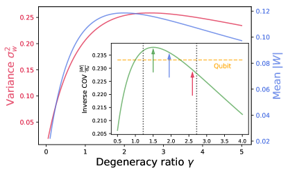
Figure 1: Average work output $|W|$, Eq. (1) (blue), its variance $\sigma^{2}_{w}$, Eq. (7) (red), and inverse coefficient of variation (COV), $|W|/\sigma_{w}$, Eq. (9) (green) (inset), for a degenerate two-level quantum Carnot engine, as a function of the degeneracy ratio $\gamma$. The maximum COV (green arrow) outperforms its nondegenerate counterpart (orange dashed line). The blue (red) arrow indicates the maximum value of the average (variance) of the work output. The vertical black dotted lines mark the respective maxima of the heat capacity (Schottky anomaly), Eq. (10), at the hot and cold bath temperatures. Parameters are $\beta_{c}=1$, $\beta_{h}=0.1$, $\omega_{2}=2$ and $\omega_{4}=1$.

Nondegenerate $N$-level system. In order to investigate the influence of the level number of the working fluid on the relative work fluctuations, we next examine a nondegenerate $N$-level system with equidistant spacing, $H_{t}=\omega_{t}\sum_{n=0}^{N-1}|n\rangle\langle n|$, as appearing in homogeneous Hamiltonians of degree $-2$ gri10 ; jar13 ; cam13 ; def14 ; bea16 . The partition function at inverse temperature $\beta$ and frequency $\omega$ is given by $Z_{N}=[1-\exp(-N\beta\omega)]/[1-\exp(-\beta\omega)]$ blu06 . The explicit (and lengthy) expressions for the heat capacity $C_{N}(\beta,\omega)$ and the entropy difference $\Delta S_{N}$ are given in the Supplemental Material sup . Compact expressions for the inverse coefficient of variation for work may be obtained in the limit of a harmonic oscillator ($N\rightarrow\infty$),

$$\left(\frac{|W|}{\sigma_{w}}\right)_{\infty}\!=\frac{\Delta S_{\infty}}{\sqrt{\left(\text{sech}(y/2)y\right)^{2}+\left(\text{sech}(x/2)x\right)^{2}}},$$ (15)

and for the case a (nondegenerate) qubit ($N=2$),

$$\!\left(\frac{|W|}{\sigma_{w}}\right)_{2}\!=\frac{\Delta S_{2}}{\sqrt{y^{2}[1-\text{tanh}(y)^{2}]+x^{2}[1-\text{tanh}(x)^{2}]}}.$$ (16)

In the high-temperature limit, $\beta_{c,h}\omega_{4,2}\ll 1$, Eq. (15) reduces to the result obtained for the classical harmonic Carnot heat engine in Ref. hol18 ,

$$\left(\frac{|W|}{\sigma_{w}}\right)_{\infty}^{\text{cl}}=\frac{\Delta S_{\infty}}{\sqrt{2}}.$$ (17)

On the other hand, the high-temperature limit of Eq. (16) exhibits a completely different $(x,y)$-dependence, which reflects the finite Hilbert space of the qubit,

$$\left(\frac{|W|}{\sigma_{w}}\right)_{2}^{\text{cl}}=\frac{\Delta S_{2}}{\sqrt{x[1-x^{2}]+y[1-y^{2}]}}.$$ (18)

Such behavior can be traced back to the properties of the heat capacity in Eq. (9): while it reaches a constant value for the (infinite-dimensional) harmonic oscillator in the classical limit (Dulong-Petit law), it vanishes for the (finite-dimensional) two-level system blu06 .

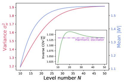
Figure 2: Average work output $|W|$, Eq. (1) (blue), its variance $\sigma^{2}_{w}$, Eq. (7) (red), and inverse coefficient of variation (COV), $|W|/\sigma_{w}$, Eq. (9) (green) (inset), for a nondegenerate $N$-level quantum Carnot engine, as a function of the level number $N$. The maximum COV outperforms both that of the two-level engine and that of the harmonic oscillator motor (violet dotted-dashed line). Same parameters as in Fig. 1.

Figure 2 displays the mean work output $|W|$ (blue), the corresponding variance $\sigma^{2}_{w}$ (red) as well as the inverse coefficient of variation (9) (green) as a function of the level number $N$. Mean and variance increase monotonously with $N$, reaching the respective values of the harmonic oscillator in the limit $N\rightarrow\infty$. However, the mean saturates faster than the variance. The inverse relative work fluctuations therefore presents a maximum that outperforms both that of the two-level engine and of the harmonic oscillator motor. Contrary to naive expectation, the $N$-level Carnot engine does thus not simply interpolate between these two extreme situations. The point of maximum inverse coefficient of variation is again different from the point of maximum work output because of increased work fluctuations. The optimal level number $\bar{N}$ satisfies the transcendental equation,

$$\left(\frac{1}{2}\partial_{N}-1\right)[C_{N}(\beta_{c},\omega_{4})+C_{N}(\beta_{h},\omega_{2})]$$

$$\quad+\left(\frac{1}{2}-\partial_{N}\right)\Delta S_{N}=0,$$ (19)

which may be solved numerically.

Degenerate $3$-level system. We finally illustrate the usefulness of Eq. (9) for determining the maximum inverse coefficient of variation for work for degenerate multilevel quantum Carnot engines by treating the case of a degenerate 3-level system with Hamiltonian $H_{t}=\omega_{t}(g_{1}\ket{1}\bra{1}+g_{2}\ket{2}\bra{2})$ and arbitrary level degeneracies $g_{n}$, $(n=0,1,2)$. The partition function at inverse temperature $\beta$ and frequency $\omega$ is here $Z_{3}=g_{0}+g_{1}e^{-\beta\omega}+g_{2}e^{-2\beta\omega}$. The corresponding inverse coefficient of variation for work (9) is represented as a function of the two degeneracy ratios $\gamma_{1}=g_{1}/g_{0}$ and $\gamma_{2}=g_{2}/g_{0}$ in Fig. 3. We identify a region of high inverse coefficient of variation for small $\gamma_{1}$ and $1\lesssim\gamma_{2}\lesssim 4$, where the quantum Carnot engine outperforms the respective nondegenerate two-level (black arrow) and three-level engines (grey arrow). We moreover notice that large ratios $\gamma_{1}$, that is, high degeneracy of the first level, is generally detrimental to the performance of the heat engine.

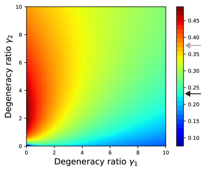
Figure 3: Inverse coefficient of variation for work, $|W|/\sigma_{w}$, Eq. (9), for a degenerate three-level quantum Carnot engine, as a function of the degeneracy ratios $\gamma_{1}$ and $\gamma_{2}$. We notice a region of high inverse coefficient of variation for small $\gamma_{1}$ and $1\lesssim\gamma_{2}\lesssim 4$, where nondegenerate two-level (black arrow) and three-level heat engines (grey arrow) are outperformed. Same parameters as in Fig. 1

Conclusions. Two-level systems and harmonic oscillators have been the models of choice for the investigations of quantum heat engines in the past decades due to their simplicity gev92 ; gev92a ; wu06 ; qua07 ; abe11 ; wan12 ; all13 ; dan20 ; abi20 . Such finite-time engines have been mostly optimized by maximizing averaged performance measures, such as mean power, with respect to cycle duration, frequency or temperature gev92 ; gev92a ; wu06 ; qua07 ; abe11 ; wan12 ; all13 ; dan20 ; abi20 . We have here extended these studies to include the effects of work fluctuations and of finite Hilbert space of the working medium, two essential features of small quantum machines. To this end, we have derived a compact expression of the relative work fluctuations of a finite-time quantum Carnot engine, as given by Eq. (9), in terms of the heat capacity of the system. We have shown that the quantum motor can outperform its nondegenerate counterparts, when optimized with respect to level degeneracy or level number. We have additionally found that optimizing the average work output, while ignoring work output fluctuations, generally leads to machines with larger instability. Our findings hence enable the analysis and future experimental realization of both high-performance and high-stability cyclic quantum heat engines.
Acknowledgements. We acknowledge financial support from the Volkswagen Foundation under project ”Quantum coins and nano sensors” and the German Science Foundation (DFG) under project FOR 2724.

Supplemental Material

Work distribution for quasistatic isotherms.
We show that quantum work is delta distributed, and therefore deterministic, during quasistatic isotherms, see Eq. (3) of the main text. This result may be derived by extending the classical derivation of Ref. hol18 to the quantum domain. We here discuss an alternative derivation by following the train of thought presented in Ref. sca20 . We begin by approximating the Hamiltonian evolution $H_{t}$ during isothermal driving as a set of $K$ discrete steps, $H_{0}\rightarrow H_{1}\rightarrow\dots\rightarrow H_{K}$. We assume the driving to be slow enough that thermal equilibrium is reached after each discrete step, so that the state of the system after the $i$-th step is of the Gibbs form, $\pi_{i}=e^{-\beta H_{i}}/Z_{i}$, at inverse temperature $\beta$. The total work distribution may then be written as a convolution of $K$ independent contributions $P_{i}(w_{i})$, $P(w)=\prod_{i=1}^{K}P_{i}(w_{i})$.

The distribution for the $i$-th quasistatic step may be obtained via the two-point-measurement scheme tal07 as,

$$P_{i}(w_{i})=\sum_{E_{i+1}^{(m)}-E_{i}^{(n)}=w_{i}}\bra{E_{i}^{(n)}}\frac{e^{-\beta H_{i}}}{Z_{i}}\ket{E_{i}^{(n)}}|\braket{E_{i}^{(n)}}{E_{i+1}^{(m)}}|^{2},$$ (20)

where $\ket{E_{i}}$ and $E_{i}$ denote the respective eigenstate and eigenenergy of the Hamiltonian $H_{i}$. The cumulant generating function (CGF),

$$G(\lambda)=\ln\int_{-\infty}^{\infty}dw~{}P(w)e^{-\beta\lambda w},$$ (21)

allows the computation of all the work cumulants via,

$$\left.\kappa_{w}^{l}=(-\beta)^{-l}\frac{d^{l}}{d\lambda^{l}}G(\lambda)\right|_{\lambda=0}.$$ (22)

Inserting Eq. (20) into Eq. (21), the CGF becomes,

$$G(\lambda) = \sum_{i=1}^{K-1}\int_{-\infty}^{\infty}dw_{i}~{}\ln P_{i}(w_{i})e^{-\beta\lambda w_{i}}$$ (23)

$$= \sum_{i=1}^{K-1}\ln\left(\text{Tr}\left[e^{-\beta\lambda H_{i+1}}e^{\beta\lambda H_{i}}\pi_{i}\right]\right)$$

$$= \sum_{i=1}^{K-1}\ln\left(\text{Tr}\left[\frac{e^{-\beta\lambda H_{i+1}}}{Z_{i+1}^{\lambda}}\frac{e^{\beta\lambda H_{i}}}{Z_{i}^{-\lambda}}\pi_{i}\right]\frac{Z_{i+1}^{\lambda}}{Z_{i}^{\lambda}}\right)$$

$$= -\beta\lambda\Delta F+\sum_{i=1}^{K-1}(\lambda-1)S_{\lambda}\left(\pi_{i+1}||\pi_{i}\right).$$

The CGF may thus be split into a protocol-independent part given by the free energy difference, $\Delta F=-\beta^{-1}\ln Z_{K}/Z_{0}$, and a protocol-dependent part given by the $\lambda$-Renyi divergence, $S_{\lambda}(\rho||\sigma)=\ln\text{Tr}[\rho^{\lambda}\sigma^{1-\lambda}]/({\lambda-1})$. Taking the limit $K\rightarrow\infty$ with ($H_{0},H_{K}$) fixed and writing the $(i+1)$-th step in terms of the $i$-th one as $H_{i+1}=H_{i}+\Delta H/K$, with $\Delta H=H_{K}-H_{0}$, the last term in Eq. (23) simplifies to,

$$\displaystyle\lim_{K\rightarrow\infty}S_{\lambda}\left(\pi_{i+1}||\pi_{i}\right) = \displaystyle\lim_{K\rightarrow\infty}\frac{1}{\lambda-1}\ln\left(\frac{\text{Tr}\left[e^{-\beta\lambda\Delta H/K}\pi_{i}\right]}{\text{Tr}\left[e^{-\beta(H_{i}+\Delta H/K)}\right]^{\lambda}\text{Tr}\left[e^{-\beta H_{i}}\right]^{-\lambda}}\right)$$ (24)

$$= \displaystyle\lim_{K\rightarrow\infty}\frac{1}{\lambda-1}\left\{\ln\left(\text{Tr}\left[e^{-\beta\lambda\Delta H/K}\pi_{i}\right]\right)-\ln\left(\frac{\text{Tr}\left[e^{-\beta H_{i}}\right]^{\lambda}}{\text{Tr}\left[e^{-\beta(H_{i}+\Delta H/K)}\right]^{\lambda}}\right)\right\}$$

$$= \frac{1}{\lambda-1}\ln\text{Tr}\left[\pi_{i}\right]=0,$$

where we have used $[H_{i},H_{i+1}]=0$ in the first line. All the terms hence vanish in the limit $K\rightarrow\infty$. As a result,

$$G(\lambda)=-\beta\lambda\Delta F.$$ (25)

The work distribution then follows as,

$$P(W)=\delta(W-\Delta F),$$ (26)

indicating that work is deterministic in this case.

Derivation of the coefficient of variation for work.
In order to derive Eqs. (8) and (9) of the main text, we first need an expression for the second moment. Integration of Eq. (6)of the main text yields,

$$\langle w^{2}\rangle = W^{2}+\langle\Delta H_{2}^{2}\rangle-\langle\Delta H_{2}\rangle^{2}+\langle\Delta H_{4}^{2}\rangle-\langle\Delta H_{4}\rangle^{2}.$$

So the work variance simply reads,

$$\sigma_{w}^{2}=\langle\Delta H_{2}^{2}\rangle-\langle\Delta H_{2}\rangle^{2}+\langle\Delta H_{4}^{2}\rangle-\langle\Delta H_{4}\rangle^{2}.$$ (28)

Using the condition, $\omega_{3}/\omega_{2}=\omega_{4}/\omega_{1}={\beta_{h}}/{\beta_{c}}$, we can simplify the mean and the square energy difference of the adiabats in terms of the canonical partition functions,

$$\sigma^{2}_{w} = \left(1-\frac{\beta_{h}}{\beta_{c}}\right)^{2}\left[\frac{1}{z_{2}}\frac{\partial^{2}}{\partial\beta_{h}^{2}}z_{2}-\frac{1}{z_{2}^{2}}\left(\frac{\partial}{\partial\beta_{h}}z_{2}\right)^{2}\right]$$ (29)

$$+ \left(1-\frac{\beta_{c}}{\beta_{h}}\right)^{2}\left[\frac{1}{z_{4}}\frac{\partial^{2}}{\partial\beta_{c}^{2}}z_{4}-\frac{1}{z_{4}^{2}}\left(\frac{\partial}{\partial\beta_{c}}z_{4}\right)^{2}\right],$$

where $z_{4}=\text{Tr}\left[e^{-\beta_{c}H_{4}}\right]$ and $z_{2}=\text{Tr}\left[e^{-\beta_{h}H_{2}}\right]$. On the other hand, the heat capacity at inverse temperature $\beta$ and frequency $\omega$ reads,

$$C(\beta,\omega) = \frac{\partial U(\beta,\omega)}{\partial T}=\beta^{2}\frac{\partial^{2}}{\partial\beta^{2}}\ln z$$

$$= \beta^{2}\left[\frac{1}{z}\frac{\partial^{2}}{\partial\beta^{2}}z-\frac{1}{z}\left(\frac{\partial z}{\partial\beta}\right)^{2}\right],$$

Combining Eqs. (29) and (30), we then obtain the coefficient of variation for work,

$$\frac{\sigma_{w}}{|W|}=\frac{\sqrt{C(\beta_{c},\omega_{4})+C(\beta_{h},\omega_{2})}}{\Delta S}.$$ (31)

The Fano factor may be similarly obtained by taking the square of the nominator of Eq. (31).

In addition, the entropy difference $\Delta S$ during the hot isotherm is given by,

$$\Delta S=\ln\frac{z_{2}}{z_{4}}+T_{h}\frac{\partial\ln z_{2}}{\partial T_{h}}-T_{c}\frac{\partial\ln z_{4}}{\partial T_{c}},$$ (32)

or, equivalently, in terms of the heat capacities,

$$\Delta S=\int_{0}^{T_{h}}dT\frac{C(1/T,\omega_{2})}{T}-\int_{0}^{T_{c}}dT\frac{C(1/T,\omega_{4})}{T}.$$ (33)

Entropy variation for harmonic oscillator and qubit.
The entropy change during the hot isotherm for the harmonic oscillator ($N\rightarrow\infty$) can be determined using the corresponding partition functions $z_{4}$ and $z_{2}$,

$$z_{4}{\Large|}_{\text{HO}}=\frac{1}{1-e^{-\beta_{c}\omega_{4}}}\text{ and }z_{2}{\Large|}_{\text{HO}}=\frac{1}{1-e^{-\beta_{h}\omega_{2}}}.$$ (34)

We find from Eq. (32),

$$\Delta S_{\infty} = -\frac{1}{2}\omega_{4}\beta_{c}\coth\left(\frac{\omega_{4}\beta_{c}}{2}\right)+\frac{1}{2}\beta_{h}\omega_{2}\coth\left(\frac{1}{2}\beta_{h}\omega_{2}\right)$$ (35)

$$- \ln\left[\text{csch}\left(\frac{\omega_{4}\beta_{c}}{2}\right)\right]+\ln\left[\text{csch}\left(\frac{1}{2}\beta_{h}\omega_{2}\right)\right].$$

Similarly, the two partition functions for the two-level system ($N=2$) are,

$$z_{4}{\Large|}_{\text{TLS}}=1-e^{-\beta_{c}\omega_{4}}\text{ and }z_{2}{\Large|}_{\text{TLS}}=1-e^{-\beta_{h}\omega_{2}}.$$ (36)

The entropy difference is accordingly,

$$\Delta S_{2} = -\omega_{4}\beta_{c}\tanh\left(\omega_{4}\beta_{c}\right)+\ln\left[\cosh\left(\omega_{4}\beta_{c}\right)\right]$$ (37)

$$+ \beta_{h}\omega_{2}\tanh\left(\beta_{h}\omega_{2}\right)-\ln\left[\cosh\left(\beta_{h}\omega_{2}\right)\right].$$

The coefficient of variation for work for the two quantum systems can eventually be evaluated using Eq. (31).

Coefficient of variation for work for a nondegenerate $N$-level system.
The partition function of a $N$-level system at arbitrary temperatures and frequencies is,

$$Z_{N}=\sum_{i=1}^{N}e^{-\beta\omega}=\frac{1-e^{-N\beta\omega}}{1-e^{-\beta\omega}}.$$ (38)

The corresponding heat capacity reads,

$$C_{N}(\beta,\omega)=\frac{\beta^{2}\omega^{2}\left[e^{\beta\omega}-N^{2}e^{\beta N\omega}-N^{2}e^{(N+2)\beta\omega}+2\left(N^{2}-1\right)e^{(N+1)\beta\omega}+e^{\beta(2N+1)\omega}\right]}{\left(e^{\beta\omega}-1\right)^{2}\left(e^{N\beta\omega}-1\right)^{2}}.$$ (39)

On the other hand, the entropy difference during the hot isotherm is given by,

$$\Delta S_{N} = -\frac{\omega_{4}\beta_{c}\left[N\left(-e^{\omega_{4}\beta_{c}}\right)+e^{N\omega_{4}\beta_{c}}+N-1\right]}{\left(e^{\omega_{4}\beta_{c}}-1\right)\left(e^{N\omega_{4}\beta_{c}}-1\right)}-\ln\left(\frac{1-e^{-N\omega_{4}\beta_{c}}}{1-e^{-\omega_{4}\beta_{c}}}\right)$$ (40)

$$+ \frac{\beta_{h}\omega_{2}\left[N\left(-e^{\beta_{h}\omega_{2}}\right)+e^{N\beta_{h}\omega_{2}}+N-1\right]}{\left(e^{\beta_{h}\omega_{2}}-1\right)\left(e^{N\beta_{h}\omega_{2}}-1\right)}+\ln\left(\frac{1-e^{-N\beta_{h}\omega_{2}}}{1-e^{-\beta_{h}\omega_{2}}}\right).$$

The coefficient of variation for work again follows by inserting Eqs. (39) and (40) into Eq. (31). We emphasize that the heat capacity and the entropy difference exhibit a non-trivial and nonmonotonous $N$-dependence, which is different from just increasing the number of particles for which the coefficient of variation would stay constant.

Coefficient of variation for work for a degenerate 3-level system.
We finally evaluate the heat capacity and the entropy change during the hot isotherm for a degenerate 3-level system $(N=3)$. The partition function is,

$$Z_{3}=g_{0}+g_{1}e^{-\beta\omega}+g_{2}e^{-2\beta\omega}.$$ (41)

The heat capacity then reads,

$$C_{3}=(\beta\omega)^{2}e^{\beta\omega}\frac{e^{2\beta\omega}\gamma_{1}+4e^{\beta\omega}\gamma_{2}+\gamma_{1}\gamma_{2}}{\left(e^{2\beta\omega}+e^{\beta\omega}\gamma_{1}+\gamma_{2}\right)^{2}},$$ (42)

with the degeneracy ratios $\gamma_{1}=g_{1}/g_{0}$ and $\gamma_{2}=g_{2}/g_{0}$. The entropy change during the hot isotherm is moreover,

$$\Delta S_{3}=\frac{\beta_{h}\omega_{2}\left(e^{\beta_{h}\omega_{2}}\gamma_{1}+2\gamma_{2}\right)}{e^{2\beta_{h}\omega_{2}}+e^{\beta_{h}\omega_{2}}\gamma_{1}+\gamma_{2}}-\frac{\beta_{c}\omega_{4}\left(e^{\beta_{c}\omega_{4}}\gamma_{1}+2\gamma_{2}\right)}{e^{2\beta_{c}\omega_{4}}+e^{\beta_{c}\omega_{4}}\gamma_{1}+\gamma_{2}}+\ln\left[\frac{1+e^{-\beta_{h}\omega_{2}}(e^{\beta_{h}\omega_{2}}\gamma_{1}+\gamma_{2})}{1+e^{-\beta_{c}\omega_{4}}(e^{\beta_{c}\omega_{4}}\gamma_{1}+\gamma_{2})}\right].$$ (43)

References

- (1) Y. A. Cengel and M. A. Boles, Thermodynamics. An Engineering Approach, (McGraw-Hill, New York, 2001).
- (2) I. A. Martinez, E. Roldan, L. Dinis, D. Petrov, J. M. R. Parrondo and R. A. Rica, Brownian Carnot engine, Nature Phys. 12, 67 (2015).
- (3) F. L. Curzon and B. Ahlborn, Efficiency of a Carnot engine at maximum power output, Am. J. Phys. 43, 22 (1975).
- (4) B. Andresen, R. S. Berry, A. Nitzan, and P. Salamon, Thermodynamics in finite time. I. The step-Carnot cycle, Phys. Rev. A 15, 2086 (1977).
- (5) D. Gutkowicz-Krusin, I. Procaccia, and J. Ross, On the efficiency of rate processes. Power and efficiency of heat engines, J. Chem. Phys. 69, 3898 (1978).
- (6) M. H. Rubin, Optimal configuration of a class of irreversible heat engines, Phys. Rev. A 19, 1272, 1277 (1979).
- (7) P. Salamon and A. Nitzan, Finite time optimizations of a Newton’s law Carnot cycle, J. Chem. Phys. 74, 3546 (1981).
- (8) M. J. Ondrechen, M. H. Rubin, and Y. B. Band, The generalized Carnot cycle: A working fluid operating in finite time between finite heat sources and sinks, J. Chem. Phys. 78, 4721 (1983).
- (9) M. Esposito, R. Kawai, K. Lindenberg, and C. Van den Broeck, Efficiency at Maximum Power of Low-Dissipation Carnot Engines, Phys. Rev. Lett. 105, 150603 (2010)
- (10) V. Cavina, A. Mari, and V. Giovannetti, Slow Dynamics and Thermodynamics of Open Quantum Systems, Phys. Rev. Lett. 119, 050601 (2017).
- (11) E. Geva and R. Kosloff, A quantum-mechanical heat engine operating in finite time. A model consisting of spin-1/2 systems as the working fluid, J. Chem. Phys. 96, 3054 (1992).
- (12) E. Geva and R. Kosloff, On the classical limit of quantum thermodynamics in finite time, J. Chem. Phys. 97 4398 (1992).
- (13) F. Wu, L. Chen, S. Wu, F. Sun and C. Wu, Performance of an irreversible quantum Carnot engine with spin1/2, J. Chem. Phys.124, 214702 (2006).
- (14) H. T. Quan, Y. Liu, C. P. Sun, F. Nori, Quantum thermodynamic cycles and quantum heat engines, Phys. Rev. E 76, 031105 (2007).
- (15) S. Abe, Maximum-power quantum-mechanical Carnot engine, Phys. Rev. E 83, 041117 (2011).
- (16) J. Wang, J. He, and Z. Wu, Efficiency at maximum power output of quantum heat engines under finite-time operation, Phys. Rev. E 85, 031145 (2012).
- (17) A. E. Allahverdyan, K. V. Hovhannisyan, A. V. Melkikh, S. G. Gevorkian, Carnot Cycle at Finite Power: Attainability of Maximal Efficiency, Phys. Rev. Lett. 111, 050601 (2013).
- (18) R. D. Dann and R. Kosloff, Quantum signatures in the quantum Carnot cycle, New J. Phys. 22, 013055 (2020).
- (19) P. Abiuso and M. Perarnau-Llobet, Optimal Cycles for Low-Dissipation Heat Engines, Phys. Rev. Lett. 124, 110606 (2020).
- (20) U. Seifert, Stochastic thermodynamics, fluctuation theorems and molecular machines, Rep. Prog. Phys. 75, 126001 (2012).
- (21) G. Verley, M. Esposito, T. Willaert, and C. V. den Broeck, The unlikely Carnot efficiency, Nature Commun. 5, 4721 (2014).
- (22) G. Verley, T. Willaert, C. Van den Broeck and M. Esposito, Universal theory of efficiency fluctuations, Phys. Rev. E 90 052145 (2014).
- (23) M. Polettini, G. Verley and M. Esposito, Efficiency Statistics at All Times: Carnot Limit at Finite Power, Phys. Rev. Lett. 114, 050601 (2015).
- (24) S. K. Manikandan, L. Dabelow, R. Eichhorn, and S. Krishnamurthy, Efficiency Fluctuations in Microscopic Machines, Phys. Rev. Lett. 122, 140601 (2019).
- (25) V. Holubec, An exactly solvable model of a stochastic heat engine: optimization of power, power fluctuations and efficiency, J. Stat. Mech. P05022 (2014);
- (26) V. Holubec and A. Ryabov, Work and power fluctuations in a critical heat engine, Phys. Rev. E 96, 030102(R) (2017).
- (27) P. Pietzonka and U. Seifert, Universal Trade-Off between Power, Efficiency and Constancy in Steady-State Heat Engines, Phys. Rev. Lett. 120, 190602 (2018).
- (28) V. Holubec and A. Ryabov, Cycling Tames Power Fluctuations near Optimum Efficiency, Phys. Rev. Lett. 121, 120601 (2018).
- (29) C. J. Foot, Atomic Physics, (Oxford University Press, Oxford, 2005).
- (30) R. L. Brooks, The Fundamentals of Atomic and Molecular Physics, (Springer, Berlin, 2013).
- (31) P. M. Chaikin and T. C. Lubensky, Principles of Condensed Matter Physics, (Cambridge University Press, Cambridge, 2000).
- (32) V. Bazani, A. Credi and M. Venturi, Molecular Devices and Machines, (Wiley-VCH, Weinheim, 2003).
- (33) S. J. Blundell and K. M. Blundell, Concepts in Thermal Physics, (Oxford University Press, Oxford, 2006).
- (34) M. Evangelisti, F. Luis, L. J. de Jongh and M. Affronte, Magnetothermal properties of molecule-based materials, J. Mater. Chem. 16, 2534 (2006).
- (35) B. Everitt, The Cambridge Dictionary of Statistics, (Cambridge University Press, Cambridge, 1998).
- (36) V. Gritsev, P. Barmettler, and E. Demler, Scaling approach to quantum non-equilibrium dynamics of many-body systems, New J. Phys. 12, 113005 (2010).
- (37) C. Jarzynski, Generating shortcuts to adiabaticity in quantum and classical dynamics, Phys. Rev. A 88, 040101(R) (2013).
- (38) A. del Campo, Shortcuts to Adiabaticity by Counterdiabatic Driving, Phys. Rev. Lett. 111, 100502 (2013).
- (39) S. Deffner, C. Jarzynski and A. del Campo, Classical and Quantum Shortcuts to Adiabaticity for Scale-Invariant Driving, Phys. Rev. X 4, 021013 (2014).
- (40) M. Beau, J. Jaramillo and A. del Campo, Scaling-Up Quantum Heat Engines Efficiently via Shortcuts to Adiabaticity, Entropy 18(5), 168 (2016).
- (41) P. Talkner, E. Lutz and P. Hänggi, Fluctuation theorems: Work is not an observable ,Phys. Rev. E 75, 050102(R).
- (42) See Supplemental Material.
- (43) A. E. Allahverdyan, R. S. Johal, and G. Mahler, Work extremum principle: Structure and function of quantum heat engines, Phys. Rev. E 77, 041118 (2008).
- (44) D. Gelbwaser-Klimovsky, W. Niedenzu, P. Brumer and G. Kurizki, Power enhancement of heat engines via correlated thermalization in a three-level ”working fluid”, Sci. Rep. 5, 14413 (2015).
- (45) W. Niedenzu, D. Gelbwaser-Klimovsky, and G. Kurizki, Performance limits of multilevel and multipartite quantum heat machines, Phys. Rev. E 92, 042123 (2015).
- (46) H. T. Quan, P. Zhang, and C. P. Sun, Quantum heat engine with multilevel quantum systems, Phys. Rev. E 72, 056110 (2005).
- (47) J. Wang and J. He, Optimization on a three-level heat engine working with two noninteracting fermions in a one-dimensional box trap, J. Appl. Phys. 111, 043505 (2012).
- (48) R. Wang, J. Wang, J. He, and Y. Ma, Performance of a multilevel quantum heat engine of an ideal -particle Fermi system, Phys. Rev. E 86, 021133 (2012).
- (49) M. Scandi, H. J. D. Miller, J. Anders and M. Perarnau-Llobet, Quantum Work statistics close to equilibrium, Phys. Rev. Research 2, 023377 (2020).