Fractional Fourier transforms on $L^{p}$ and applications

Abstract

This paper is devoted to the $L^{p}(\mathbb{R})$ theory of the fractional Fourier transform (FRFT) for $1\leq p<2$. In view of the special structure of the FRFT, we study FRFT properties of $L^{1}$ functions, via the introduction of a suitable chirp operator. However, in the $L^{1}(\mathbb{R})$ setting, problems of convergence arise even when basic manipulations of functions are performed. We overcome such issues and study the FRFT inversion problem via approximation by suitable means, such as the fractional Gauss and Abel means. We also obtain the regularity of fractional convolution and results on pointwise convergence of FRFT means. Finally we discuss $L^{p}$ multiplier results and a Littlewood-Paley theorem associated with FRFT.

3.5cm3cm3cm3cm

1 Introduction

In classical Fourier analysis three important classes of operators arise: maximal averages, singular integrals, and oscillatory integrals. The Hardy-Littlewood maximal operator, the Hilbert transform and the Fourier transform, respectively, are prime examples of these classes of operators. In recent decades fractional versions of the first two types of operators have been widely studied, but less attention has been paid to the mathematical theory of the fractional Fourier transform. In this paper we undertake this task, which is strongly motivated by the important role it plays in practical applications.

The Fourier transform is one of the most important and powerful tools in theoretical and applied mathematics. Mainly driven by the need to analyze and process non-stationary signals, the Fourier transform of fractional order has been proposed and developed by several scholars. At present, the fractional Fourier transform (FRFT for short) has found applications in many aspects of scientific research and engineering technology, such as swept filter, artificial neural network, wavelet transform, time-frequency analysis, time-varying filtering, complex transmission and so on (see, e.g., [21, 23, 3, 16, 13, 20]). In addition, it was also used widely in fields of solving partial differential equations (cf., [15, 10]), quantum mechanics (cf., [15, 19]), diffraction theory and optical transmission (cf., [18]), optical system and optical signal processing (cf., [1, 17, 9]), optical image processing (cf., [10, 9]), etc.

The FRFT is a fairly old mathematical topic. It dates back to work by Wiener [24] in 1929, but it was not until the past three decades that significant attention was paid to this object starting with Namias’ work [15] in 1980. The approach used by Namias relies primarily on eigenfunction expansions. For suitable functions $f$ on the line, the classical Fourier transform $\mathcal{F}$ is defined as follows

$$(\mathcal{F}f)(x)=\int_{-\infty}^{+\infty}f(t)e^{-2\pi ixt}\mathrm{d}t.$$ (1.1)

It is known that $\mathcal{F}$ is a homeomorphism on $L^{2}(\mathbb{R})$ and has eigenvalues

$$\lambda_{n}=e^{in\pi/2},\quad n=0,1,2,\ldots.$$

with corresponding eigenfunctions

$$\psi_{n}(x)=e^{-x^{2}/2}H_{n}(x),$$

where $H_{n}$ is the Hermite polynomial of degree $n$ (see [5]). Since $\{\psi_{n}\}$ is an orthonrmal basis of $L^{2}(\mathbb{R})$, it follows that

$$\mathcal{F}f=\sum_{n}e^{-in\pi/2}(f,\psi_{n})_{2}\psi_{n},\quad\forall f\in L^{2}(\mathbb{R}).$$

This naturally leads to the definition of the fractional order operators $\{\mathcal{F}_{\alpha}\}$ for $\alpha\in\mathbb{R}$ via

$$\mathcal{F}_{\alpha}f=\sum_{n}e^{-in\alpha}(f,\psi_{n})_{2}\psi_{n},\quad\forall f\in L^{2}(\mathbb{R}).$$

It is clear that $\mathcal{F}_{\alpha}=\mathcal{F}$ when $\alpha=\pi/2$.

In 1987, McBride and Kerr [11] provided a rigorous definition on the Schwartz space $S(\mathbb{R})$ of the FRFT in integral form based on a modification of Namias’ fractional operators. For $\left|\alpha\right|\in\left(0,\pi\right)$, McBride and Kerr [11] defined the FRFT by

$$(\mathcal{F}_{\alpha}f)(x)=\frac{e^{i\left(\hat{\alpha}\pi/4-\alpha/2\right)}}{\sqrt{\left|\sin\alpha\right|}}e^{i\pi x^{2}\cot\alpha}\int_{-\infty}^{+\infty}f(t)e^{-\pi i(2xt\csc\alpha-t^{2}\cot\alpha)}\mathrm{d}t,$$ (1.2)

where $\hat{\alpha}=\mathrm{sgn}\left(\sin\alpha\right)$. The definition extends to all $\alpha\in\mathbb{R}$ by periodicity. Moreover, these authors proved that

Theorem 1.1 ([11]).

For all $f\in S(\mathbb{R})$ and all $\alpha,\beta\in\mathbb{R}$ we have

1. $\mathcal{F}_{\alpha}:S(\mathbb{R})\rightarrow S(\mathbb{R})$ is a homeomorphism;

2. $\mathcal{F}_{\alpha}\mathcal{F}_{\beta}f=\mathcal{F}_{\alpha+\beta}f$.

Later, Kerr [8] studied the $L^{2}(\mathbb{R})$ theory of $\mathcal{F}_{\alpha}$. He gave the definition of FRFT on $L^{2}(\mathbb{R})$ by interpreting (1.2) as follows:

$$(\mathcal{F}_{\alpha}f)(x)=\frac{e^{i\left(\hat{\alpha}\pi/4-\alpha/2\right)}}{\sqrt{\left|\sin\alpha\right|}}e^{i\pi x^{2}\cot\alpha}\lim_{R\rightarrow\infty}\int_{-R}^{R}f(t)e^{-\pi i(2xt\csc\alpha-t^{2}\cot\alpha)}\mathrm{d}t$$ (1.3)

and proved the following result.

Theorem 1.2 ([8]).

For all $f,g\in L^{2}(\mathbb{R})$ and all $\alpha,\beta\in\mathbb{R}$ we have

1. $\mathcal{F}_{\alpha}:L^{2}(\mathbb{R})\rightarrow L^{2}(\mathbb{R})$ is a homeomorphism;

2. $\left\|\mathcal{F}_{\alpha}f\right\|_{2}=\left\|f\right\|_{2}$;

3. $\mathcal{F}_{\alpha}\mathcal{F}_{\beta}f=\mathcal{F}_{\alpha+\beta}f$;

4. $\int_{-\infty}^{+\infty}(\mathcal{F}_{\alpha}f)(x)g(x)\mathrm{d}x=\int_{-\infty}^{+\infty}f(x)(\mathcal{F}_{\alpha}g)(x)\mathrm{d}x$;

5. $\{\mathcal{F}_{\alpha}:\alpha\in\mathbb{R}\}$ is a strongly continuous unitary group of operators on $L^{2}(\mathbb{R)}$.

For additional work in this area, refer to [6, 14], etc..

In an attempt to take the theory of FRFT beyond $S(\mathbb{R})$ or $L^{2}(\mathbb{R)}$, we discuss in this paper (Section 4) the behavior of FRFT on $L^{p}(\mathbb{R})$ for $1\leq p<2$. In Section 2, we discuss the elementary properties of FRFT on $L^{1}(\mathbb{R})$. Section 3 is devoted to the problem of FRFT inversion, which is established via an approximation in terms of FRFT integral means. In Section 5, we discuss $L^{p}$ multiplier results and a Littlewood-Paley theorem associated with FRFT. Using the language of time-frequency analysis, this means that an $L^{1}$ chirp signal, whose FRFT is non-integrable, is recovered from the frequency domain as a limit of the inverted Abel means of its FRFT; this is discussed in the last section.

2 FRFT on $L^{1}(\mathbb{R})$

It is natural to begin our exposition by defining the FRFT on $L^{1}(\mathbb{R})$; our definition is like that in [11]. In $L^{1}(\mathbb{R})$, problems of convergence arise when certain manipulations of functions are performed and FRFT inversion is not possible.

Definition 2.1.

For $f\in L^{1}(\mathbb{R})$ and $\alpha\in\mathbb{R}$, the fractional Fourier transform of order $\alpha$ of $f$ is defined by

$$(\mathcal{F}_{\alpha}f)(x)=\left\{\begin{array}[c]{ll}\int_{-\infty}^{+\infty}K_{\alpha}(x,t)f(t)\,\mathrm{d}t,&\alpha\neq n\pi,\quad n\in\mathbb{N},\\ f(x),&\alpha=2n\pi,\\ f(-x),&\alpha=(2n+1)\pi,\end{array}\right.$$ (2.1)

where

$$K_{\alpha}(x,t)=A_{\alpha}\exp\left[2\pi i\left(\frac{t^{2}}{2}\cot\alpha-xt\csc\alpha+\frac{x^{2}}{2}\cot\alpha\right)\right]$$

is the kernel of FRFT and

$$A_{\alpha}=\sqrt{1-i\cot\alpha}.$$ (2.2)

As the parameter $\alpha$ only appears as an argument of trigonometric functions (see (2.1)), it follows that $\mathcal{F}_{\alpha}$ is $2\pi$-periodic with respect to $\alpha$. Hence, throughout this paper we shall always assume $\alpha\in[0,2\pi)$.

Figure 2.1: rotation of time-frequency domain

Notice now that when $n\in\mathbb{Z}$, $\mathcal{F}_{n\pi/2}f=\mathcal{F}^{n}f$, where $\mathcal{F}^{n}$ is the $n$th power of the classical Fourier operator (1.1). Therefore, $\mathcal{F}_{\alpha}$ can be regarded as the $s$th power of the Fourier transform, where $s=2\alpha/\pi$, that is,

$$\mathcal{F}^{s}f=\mathcal{F}_{s\pi/2}f.$$

Denote by $\mathcal{I}$ the identity operator and $\mathcal{P}$ the reflection operator defined by $\mathcal{P}g(x)=g(-x)$. We can easily see that (Figure 2.1)

$$\mathcal{F}^{0}=\mathcal{F}_{0}=\mathcal{I};$$

$$\mathcal{F}^{1}=\mathcal{F}_{\pi/2}=\mathcal{F};$$

$$\mathcal{F}^{2}=\mathcal{F}_{\pi}=\mathcal{P};$$

$$\mathcal{F}^{3}=\mathcal{F}_{3\pi/2}=\mathcal{FP=PF};$$

$$\mathcal{F}^{4}=\mathcal{F}_{2\pi}=\mathcal{F}^{0}=\mathcal{I};$$

$$\mathcal{F}^{4n\pm s}=\mathcal{F}_{2n\pi\pm\alpha}=\mathcal{F}_{\pm\alpha}=\mathcal{F}^{\pm s}.$$

Every signal (or function) can be described indirectly and uniquely by a Wigner distribution function (WDF). The classical Fourier transform $\mathcal{F}$ lets the WDF rotate by an angle of $\pi/2$. Hence, $\mathcal{F}u$ is the function corresponding to the WDF obtained by rotating the original WDF of $u$ by an angle $\pi/2$. Analogously, the FRFT of order $\alpha$ is the unique function whose WDF is obtained by rotating the original WDF of $u$ by an angle $\alpha$. We refer to [10] for more details on this.

Example 2.1.

Define the following function on the line:

$$f=\sum_{n=1}^{\infty}n\chi_{[n,n+\frac{1}{n^{3}})}.$$

Using (2.1), we can easily calculate the FRFT of this function:

$$\left(\mathcal{F}_{\alpha}f\right)(x)=\frac{A_{\alpha}e^{i\pi x^{2}\cot\alpha}}{2\pi ix}\sum\limits_{n=1}^{\infty}ne^{-2n\pi ix}\left(1-e^{-\frac{2\pi ix}{n^{3}}}\right),$$

where $A_{\alpha}$ is as in (2.2). This function lies in $L^{1}(\mathbb{R})$ but not in $L^{2}(\mathbb{R})$ as

$$\int_{-\infty}^{+\infty}\left|f(t)\right|\mathrm{d}t=\sum\limits_{n=1}^{\infty}\int_{n}^{n+\frac{1}{n^{3}}}n\,\mathrm{d}t=\sum\limits_{n=1}^{\infty}\frac{1}{n^{2}}=\frac{\pi^{2}}{6}<\infty$$

and

$$\int_{-\infty}^{+\infty}\left|f(t)\right|^{2}\mathrm{d}t=\sum\limits_{n=1}^{\infty}\int_{n}^{n+\frac{1}{n^{3}}}n^{2}\,\mathrm{d}t=\sum\limits_{n=1}^{\infty}\frac{1}{n}=\infty.$$

Remark 2.1.

Define the chirp operator $\mathcal{M}_{\alpha}$ acting on functions $\phi$ in $L^{1}(\mathbb{R})$ as follows:

$$\mathcal{M}_{\alpha}\phi(x)=e^{\pi ix^{2}\cot\alpha}\phi(x).$$

Then for $\alpha\neq n\pi$, let $A_{\alpha}$ be as in (2.2). Then the FRFT of $f\in L^{1}(\mathbb{R})$ can be written as

$$(\mathcal{F}_{\alpha}f)(x) =A_{\alpha}e^{i\pi x^{2}\cot\alpha}\mathcal{F}[e^{i\pi t^{2}\cot\alpha}f(t)](x\csc\alpha)$$

$$=A_{\alpha}\mathcal{M}_{\alpha}\mathcal{F}[\mathcal{M}_{\alpha}f(t)](x\csc\alpha).$$ (2.3)

In view of (2.3), we see that the FRFT of a function (or signal) $u(t)$ can be decomposed into four simpler operators, according to the diagram of Figure 2.2:

1. multiplication by a chirp signal, $g(t)=e^{\pi it^{2}\cot\alpha}u(t)$;

2. Fourier transform, $\hat{g}(x)=(\mathcal{F}g)(x)$;

3. scaling, $\tilde{g}(x)=\hat{g}(x\csc\alpha)$;

4. multiplication by a chirp signal, $(\mathcal{F}_{\alpha}u)(x)=A_{\alpha}e^{\pi ix^{2}\cot\alpha}\tilde{g}(x)$.

Figure 2.2: the decomposition of the FRFT

In view of the decomposition (2.3) of the FRFT, the boundedness properties of the fractional Fourier operator $\mathcal{F}_{\alpha}$ is largely the same of the classical Fourier operator $\mathcal{F}$. However, due to the factors $e^{i\pi x^{2}\cot\alpha}$and $e^{i\pi t^{2}\cot\alpha}$, the convergence properties are not trival. We now discuss some basic properties of the FRFT on $L^{1}(\mathbb{R})$.

Firstly, we consider the behavior of FRFT at infinity. The following is the fractional version of the Riemann-Lebesgue lemma.

Lemma 2.2 (Riemann-Lebesgue lemma).

For $f\in L^{1}(\mathbb{R})$, we have that

$$\left|\left(\mathcal{F}_{\alpha}f\right)(x)\right|\rightarrow 0$$

as $x\rightarrow\infty$.

Proof.

Since $\mathcal{M}_{\alpha}f\in L^{1}(\mathbb{R})$, then $|\mathcal{F}(\mathcal{M}_{\alpha}f)(x)|\rightarrow 0$ as $x\rightarrow\infty$ by the Riemann-Lebesgue lemma for the classical Fourier transform. Hence, it follows from (2.3) and the boundedness of $\mathcal{M}_{\alpha}$ that

$$|\left(\mathcal{F}_{\alpha}f\right)(x)|=|A_{\alpha}\mathcal{M}_{\alpha}\mathcal{F}(\mathcal{M}_{\alpha}f)(x\csc\alpha)|\rightarrow 0$$

as $x\rightarrow\infty$. ∎

Proposition 2.3.

The following statements are valid:

1. The FRFT $\mathcal{F}_{\alpha}$ is a bounded linear operator from $L^{1}(\mathbb{R})\rightarrow L^{\infty}(\mathbb{R})$.

2. For $f\in L^{1}(\mathbb{R})$, $\mathcal{F}_{\alpha}f$ is uniformly continuous on $\mathbb{R}$.

Proof.

(i) It is obvious that $\mathcal{F}_{\alpha}$ is linear. Moreover the claimed boundedness holds as

$$\left\|\mathcal{F}_{\alpha}f\right\|_{\infty}=|A_{\alpha}|\left\|\mathcal{F}(\mathcal{M}_{\alpha}f)\right\|_{\infty}\leq|A_{\alpha}|\left\|\mathcal{M}_{\alpha}f\right\|_{1}=|A_{\alpha}|\left\|f\right\|_{1}.$$

(ii) For an arbitrary $\varepsilon>0$, it follows from Lemma 2.2 that there exists $\eta>0$ such that for every $x_{i}\in\mathbb{R}\setminus[-\eta,\eta]$, $|\left(\mathcal{F}_{\alpha}f\right)(x_{i})|<\varepsilon/2,i=1,2$. Thus

$$\left|\left(\mathcal{F}_{\alpha}f\right)(x_{1})-\left(\mathcal{F}_{\alpha}f\right)(x_{2})\right|<\varepsilon.$$

For every $x_{1},x_{2}\in[-\eta-1,\eta+1]$, by the Lagrange mean value theorem, there exists $\xi$ between $x_{1}$ and $x_{2}$ such that

$$K_{\alpha}(x_{1},t)-K_{\alpha}(x_{2},t) =\frac{\partial}{\partial x}K_{\alpha}\left(\xi,t\right)\left(x_{1}-x_{2}\right)$$

$$=2\pi iA_{a}\left(\xi\cot\alpha-t\csc\alpha\right)K_{\alpha}\left(\xi,t\right)\left(x_{1}-x_{2}\right).$$

There exist $N>0$ such that for $\left|t\right|\geq N$,

$$\int_{\left|t\right|\geq N}\left|f\left(t\right)\right|\mathrm{d}t<\frac{\varepsilon}{4}.$$

Hence,

$$\left|\left(\mathcal{F}_{\alpha}f\right)\left(x_{1}\right)-\left(\mathcal{F}_{\alpha}f\right)\left(x_{2}\right)\right| =\left|\int_{-\infty}^{+\infty}\left(K_{\alpha}(x_{1},t)f(t)-K_{\alpha}(x_{2},t)f(t)\right)\mathrm{d}t\right|$$

$$\leq 2\int_{\left|t\right|\geq N}\left|f\left(t\right)\right|\mathrm{d}t+\left|\int_{\left|t\right|\leq N}f(t)\left(K_{\alpha}(x_{1},t)-K_{\alpha}(x_{2},t)\right)\mathrm{d}t\right|$$

$$<\frac{\varepsilon}{2}+2\pi|A_{\alpha}|\int_{\left|t\right|\leq N}\left|f(t)\right|\left|\xi\cot\alpha-t\csc\alpha\right|\left|x_{1}-x_{2}\right|\mathrm{d}t$$

$$<\frac{\varepsilon}{2}+C\left|x_{1}-x_{2}\right|\int_{\left|t\right|\leq N}\left|f(t)\right|\mathrm{d}t$$

$$\leq\frac{\varepsilon}{2}+C\left|x_{1}-x_{2}\right|\left\|f\right\|_{1},$$

where $C$ is a constant independent of $x_{1},x_{2}$. Then for

$$\left|x_{1}-x_{2}\right|<\frac{\varepsilon}{2C\left\|f\right\|_{1}}.$$

we obtain

$$\left|\left(\mathcal{F}_{\alpha}f\right)\left(x_{1}\right)-\left(\mathcal{F}_{\alpha}f\right)\left(x_{2}\right)\right|<\varepsilon.$$

So, we conclude that $\mathcal{F}_{\alpha}f$ is uniformly continuous on $\mathbb{R}$. ∎

Lemma 2.2 and Proposition 2.3 imply that

$$f\in L^{1}(\mathbb{R})\Rightarrow\mathcal{F}_{\alpha}f\in C_{0}(\mathbb{R}).$$ (2.4)

A natural question is whether the reverse implication to (2.4) holds, precisely,

Question. Given $g\in C_{0}(\mathbb{R})$, is there a $L^{1}$-function $f$ such that $\mathcal{F}_{\alpha}f=g$?

The answer to this question is negative as the following example illustrates.

Example 2.2.

Let

$$g(x)=\left\{\begin{array}[c]{ll}\left(\ln x\right)^{-1}e^{\pi ix^{2}\cot\alpha},&x\geq e,\\ xe^{\pi ix^{2}\cot\alpha-1},&-e<x<e,\\ -\left(\ln(-x)\right)^{-1}e^{\pi ix^{2}\cot\alpha},&x\leq-e.\end{array}\right.$$

Then $g\in C_{0}(\mathbb{R})$ and $g$ is not the FRFT of any $L^{1}$-function. To show this, we need first to prove the following.

Claim.

If $f\in L^{1}(\mathbb{R})$ and $\mathcal{F}_{\alpha}f$ is odd, then

$$\left|\int_{\varepsilon}^{N}\frac{(\mathcal{F}_{\alpha}f)(x)}{x}e^{-\pi ix^{2}\cot\alpha}\mathrm{d}x\right|\leq 4\left|A_{\alpha}\right|\left\|f\right\|_{1}$$

for all $N>\varepsilon>0$.

Indeed, since $\mathcal{F}_{\alpha}f$ is odd, we have

$$\left(\mathcal{F}_{\alpha}f\right)(x) =\frac{1}{2}\left(\left(\mathcal{F}_{\alpha}f\right)(x)-\left(\mathcal{F}_{\alpha}f\right)(-x)\right)$$

$$=\frac{1}{2}\int_{-\infty}^{+\infty}f(t)\left(K_{\alpha}(x,t)-K_{\alpha}(-x,t)\right)\mathrm{d}t$$

$$=\frac{A_{\alpha}}{2}\int_{-\infty}^{+\infty}f(t)e^{\pi i\left(t^{2}+x^{2}\right)\cot\alpha}\left(e^{-2\pi ixt\csc\alpha}-e^{2\pi ixt\csc\alpha}\right)\mathrm{d}t$$

$$=-iA_{\alpha}e^{\pi ix^{2}\cot\alpha}\int_{-\infty}^{+\infty}f(t)e^{\pi it^{2}\cot\alpha}\sin\left(2\pi xt\csc\alpha\right)\mathrm{d}t.$$

Then

$$\int_{\varepsilon}^{N}\frac{(\mathcal{F}_{\alpha}f)(x)}{x}e^{-\pi ix^{2}\cot\alpha}\mathrm{d}x =-iA_{\alpha}\int_{\varepsilon}^{N}\frac{1}{x}\left(\int_{-\infty}^{+\infty}f(t)e^{\pi it^{2}\cot\alpha}\sin\left(2\pi xt\csc\alpha\right)\mathrm{d}t\right)\mathrm{d}x$$

$$=-iA_{\alpha}\int_{-\infty}^{+\infty}f(t)e^{\pi it^{2}\cot\alpha}\left(\int_{2\pi\varepsilon t\csc\alpha}^{2\pi Nt\csc\alpha}\frac{\sin x}{x}\mathrm{d}x\right)\mathrm{d}t.$$

Note that

$$\left|\int_{2\pi\varepsilon t\csc\alpha}^{2\pi Nt\csc\alpha}\frac{\sin x}{x}\mathrm{d}x\right|\leq 4,\quad\forall~{}0<\varepsilon<N<+\infty.$$

Consequently,

$$\left|\int_{\varepsilon}^{N}\frac{(\mathcal{F}_{\alpha}f)(x)}{x}e^{-\pi ix^{2}\cot\alpha}\mathrm{d}x\right| \leq\left|A_{\alpha}\right|\int_{-\infty}^{+\infty}\left|f(t)\right|\left|\int_{2\pi\varepsilon t\csc\alpha}^{2\pi Nt\csc\alpha}\frac{\sin x}{x}\mathrm{d}x\right|\mathrm{d}t$$

$$\leq 4\left|A_{\alpha}\right|\left\|f\right\|_{1}.$$

So the claim holds. Since $g\in C_{0}(\mathbb{R})$ is an odd function and

$$\lim_{\begin{subarray}{c}t\rightarrow\infty\\ \varepsilon\rightarrow 0^{+}\end{subarray}}\left|\int_{\varepsilon}^{t}\frac{g(x)}{x}e^{-\pi ix^{2}\cot\alpha}\mathrm{d}x\right|=\infty,$$

the above claim implies that $g$ is not the FRFT of any $L^{1}$-function.

We conclude this section with a useful identity.

Theorem 2.4 (Multiplication formula).

For every $f,g\in L^{1}(\mathbb{R})$ and $\alpha\in\mathbb{R}$ we have

$$\int_{-\infty}^{+\infty}(\mathcal{F}_{\alpha}f)(x)g(x)\mathrm{d}x=\int_{-\infty}^{+\infty}f(x)(\mathcal{F}_{\alpha}g)(x)\mathrm{d}x.$$ (2.5)

Proof.

The identity (2.5) is an immediate consequence of Fubini’s theorem. Indeed,

$$\int_{-\infty}^{+\infty}(\mathcal{F}_{\alpha}f)(x)g(x)\mathrm{d}x =\int_{-\infty}^{+\infty}g(x)\left(\int_{-\infty}^{+\infty}f(t)K_{\alpha}\left(x,t\right)\mathrm{d}t\right)\mathrm{d}x$$

$$=\int_{-\infty}^{+\infty}f(t)\left(\int_{-\infty}^{+\infty}g(x)K_{\alpha}\left(x,t\right)\mathrm{d}x\right)\mathrm{d}t$$

$$=\int_{-\infty}^{+\infty}f(x)(\mathcal{F}_{\alpha}g)(x)\mathrm{d}x,$$

noting that $K_{\alpha}$ is a bounded function and $K_{\alpha}\left(x,t\right)=K_{\alpha}\left(t,x\right)$ for all $x$ and $t$. ∎

3 Fractional approximate identities and FRFT inversion on $L^{1}(\mathbb{R})$

In this section, we study FRFT inversion. Namely, given the FRFT of an $L^{1}$-function, how to recover the original function? We naturally hope that the integral

$$\int_{-\infty}^{+\infty}(\mathcal{F}_{\alpha}f)(x)K_{-\alpha}(x,t)\mathrm{d}x$$ (3.1)

equals $f(t)$. Unfortunately, when $f$ is integrable, one may not necessarily have that $\mathcal{F}_{\alpha}f$ is integrable, so the integral (3.1) may not make sense. In fact, $\mathcal{F}_{\frac{\pi}{2}}f$ is nonintegrable in general (cf., [4, pp. 12]).

Example 3.1.

Let

$$f(t)=\left\{\begin{array}[c]{cc}e^{-\pi\left(2t+it^{2}\cot\alpha\right)},&t\geq 0,\\ 0,&t<0.\end{array}\right.$$

Then $f\in L^{1}(\mathbb{R})$ but

$$\left(\mathcal{F}_{\alpha}f\right)(x)=\frac{A_{\alpha}e^{\pi ix^{2}\cot\alpha}}{2\pi\left(1+ix\right)}\notin L^{1}(\mathbb{R}).$$

To overcome this difficulty, we employ integral summability methods. We introduce the fractional convolution and we establish the approximate identities in the fractional setting. Then we study the $\Phi_{\alpha}$ means of the fractional Fourier integral, especially Abel means and Gauss means. Based on the regularity of the fractional convolution and the results of pointwise convergence, we can approximate $f$ by the $\Phi_{\alpha}$ means of the integral (3.1).

3.1 Fractional convolution and approximate identities

Definition 3.1.

Let $f,g$ be in $L^{1}(\mathbb{R})$. Define the fractional convolution of order $\alpha$ by

$$\left(f\overset{\alpha}{\ast}g\right)(x)=e^{-\pi ix^{2}\cot\alpha}\int_{-\infty}^{+\infty}e^{\pi it^{2}\cot\alpha}f(t)g(x-t)\mathrm{d}t=\mathcal{M}_{-\alpha}\left(\mathcal{M}_{\alpha}f\ast g\right)(x).$$

We reserve the following notation for the $L^{1}$ dilation of a function $\phi$

$$\phi_{\varepsilon}(x):=\frac{1}{\varepsilon}\phi\left(\frac{x}{\varepsilon}\right),\quad\forall\varepsilon>0.$$

The following is a fundamental result concerning fractional convolution and approximate identities.

Theorem 3.2.

Let $\phi\in L^{1}(\mathbb{R})$ and $\int_{-\infty}^{+\infty}\phi\left(x\right)\mathrm{d}x=1$. If $f\in L^{p}\left(\mathbb{R}\right),1\leq p<\infty$, then

$$\lim_{\varepsilon\rightarrow 0}\left\|\left(f\overset{\alpha}{\ast}\phi_{\varepsilon}\right)-f\right\|_{p}=0.$$

Proof.

Note that

$$\left(f\overset{\alpha}{\ast}\phi_{\varepsilon}\right)(x)-f(x) =e^{-\pi ix^{2}\cot\alpha}\int_{-\infty}^{+\infty}e^{\pi it^{2}\cot\alpha}f(t)\phi_{\varepsilon}(x-t)\mathrm{d}t-\int_{-\infty}^{+\infty}\phi_{\varepsilon}\left(t\right)f\left(x\right)\mathrm{d}t$$

$$=\int_{-\infty}^{+\infty}\left(e^{\pi i\left(\left(x-t\right)^{2}-x^{2}\right)\cot\alpha}f(x-t)-f\left(x\right)\right)\phi_{\varepsilon}(t)\mathrm{d}t.$$

By Minkowski’s integral inequality, we obtain

$$\left\|\left(f\overset{\alpha}{\ast}\phi_{\varepsilon}\right)-f\right\|_{p} =\left(\int_{-\infty}^{+\infty}\left|\int_{-\infty}^{+\infty}\left(e^{\pi i\left(\left(x-t\right)^{2}-x^{2}\right)\cot\alpha}f(x-t)-f\left(x\right)\right)\phi_{\varepsilon}(t)\mathrm{d}t\right|^{p}\mathrm{d}x\right)^{\frac{1}{p}}$$

$$\leq\int_{-\infty}^{+\infty}\left(\int_{-\infty}^{+\infty}\left|e^{\pi i\left(\left(x-t\right)^{2}-x^{2}\right)\cot\alpha}f(x-t)-f\left(x\right)\right|^{p}\mathrm{d}x\right)^{\frac{1}{p}}\left|\phi_{\varepsilon}(t)\right|\mathrm{d}t$$

$$=\int_{-\infty}^{+\infty}\left(\int_{-\infty}^{+\infty}\left|e^{\pi i\left(\left(x-\varepsilon t\right)^{2}-x^{2}\right)\cot\alpha}f(x-\varepsilon t)-f\left(x\right)\right|^{p}\mathrm{d}x\right)^{\frac{1}{p}}\left|\phi(t)\right|\mathrm{d}t.$$

We first prove that

$$J_{\varepsilon}:=\left(\int_{-\infty}^{+\infty}\left|e^{\pi i\left(\left(x-\varepsilon t\right)^{2}-x^{2}\right)\cot\alpha}f(x-\varepsilon t)-f\left(x\right)\right|^{p}\mathrm{d}x\right)^{\frac{1}{p}}\rightarrow 0$$ (3.2)

as $\varepsilon\rightarrow 0$.

In fact, for an arbitrary $\eta>0$, since the space of continuous functions with compact support $C_{c}\left(\mathbb{R}\right)$ is dense in $L^{p}(\mathbb{R})$, there exists $g\in C_{c}\left(\mathbb{R}\right)$ such that

$$\left\|f-g\right\|_{p}<\frac{\eta}{2}.$$

Since $g$ is uniformly continuous,

$$\lim_{\varepsilon\rightarrow 0}\left|g\left(x-\varepsilon t\right)-g\left(x\right)\right|=0.$$

Note that

$$\left|J_{\varepsilon}\right|\leq \left\|e^{\pi i\left(\left(\left(\cdot\right)-\varepsilon t\right)^{2}-\left(\cdot\right)^{2}\right)\cot\alpha}f(\left(\cdot\right)-\varepsilon t)-e^{\pi i\left(\left(\left(\cdot\right)-\varepsilon t\right)^{2}-\left(\cdot\right)^{2}\right)\cot\alpha}g(\left(\cdot\right)-\varepsilon t)\right\|_{p}$$

$$+\left\|e^{\pi i\left(\left(\left(\cdot\right)-\varepsilon t\right)^{2}-\left(\cdot\right)^{2}\right)\cot\alpha}g(\left(\cdot\right)-\varepsilon t)-g(\left(\cdot\right)-\varepsilon t)\right\|_{p}$$

$$+\left\|g(\left(\cdot\right)-\varepsilon t)-g\right\|_{p}+\left\|f-g\right\|_{p}$$

$$= 2\left\|f-g\right\|_{p}+\left\|g\right\|_{\infty}\left\|e^{\pi i\left(\left(\left(\cdot\right)-\varepsilon t\right)^{2}-\left(\cdot\right)^{2}\right)\cot\alpha}-1\right\|_{p}+\left\|g(\left(\cdot\right)-\varepsilon t)-g\right\|_{p}.$$

Consequently, it follows from Lebesgue’s dominated convergence theorem that

$$\varlimsup_{\varepsilon\rightarrow 0}\left|J_{\varepsilon}\right|\leq \eta+\varlimsup_{\varepsilon\rightarrow 0}\left\|g(\left(\cdot\right)-\varepsilon t)-g\right\|_{p}$$

$$+\left\|g\right\|_{\infty}\varlimsup_{\varepsilon\rightarrow 0}\left\|e^{\pi i\left(\left(\left(\cdot\right)-\varepsilon t\right)^{2}-\left(\cdot\right)^{2}\right)\cot\alpha}-1\right\|_{p}=\eta.$$

Therefore (3.2) holds. In view of

$$\left(\int_{-\infty}^{+\infty}\left|e^{\pi i\left(\left(x-\varepsilon t\right)^{2}-x^{2}\right)\cot\alpha}f(x-\varepsilon t)-f\left(x\right)\right|^{p}\mathrm{d}x\right)^{\frac{1}{p}}\leq 2\left\|f\right\|_{p}<\infty,$$

and using Lebesgue’s dominated convergence theorem again, we deduce that

$$\lim_{\varepsilon\rightarrow 0}\left\|\left(f\overset{\alpha}{\ast}\phi_{\varepsilon}\right)-f\right\|_{p}=0.$$

∎

Next, we discuss the pointwise convergence of approximate identities with respect to fractional convolution.

Theorem 3.3.

Let $\phi\in L^{1}(\mathbb{R})$ and $\int_{-\infty}^{+\infty}\phi\left(x\right)\mathrm{d}x=1$. Denote the decreasing radial dominant functions of $\phi$ by $\psi\left(x\right)=\underset{\left|t\right|\geq\left|x\right|}{\sup}\left|\phi\left(t\right)\right|$. If $\psi\in L^{1}(\mathbb{R})$ and $f\in L^{p}(\mathbb{R}),1\leq p<\infty$, then

$$\lim_{\varepsilon\rightarrow 0}\left(f\overset{\alpha}{\ast}\phi_{\varepsilon}\right)\left(x\right)=f\left(x\right),\quad\mathrm{a.e.}\quad x\in\mathbb{R}.$$

Proof.

Since $\psi$ is decreasing and nonnegative, we have

$$\left|x\psi(x)\right|\leq 2\left|\int_{x/2}^{x}\psi(s)\mathrm{d}s\right|\rightarrow 0$$

as $x\rightarrow 0$ or $x\rightarrow\infty$. Moreover, there is a constant $A>0$ such that

$$\left|x\psi(x)\right|\leq A,\quad\forall x\in\mathbb{R}.$$

As $\mathcal{M}_{\alpha}f\in L^{p}(\mathbb{R})$, it follows from Lebesgue’s differentiation theorem that, for almost all $x\in\mathbb{R}$ we have

$$\lim_{r\rightarrow 0}\frac{1}{r}\int_{-r}^{r}\left|e^{\pi i\left(x-t\right)^{2}\cot\alpha}f\left(x-t\right)-e^{\pi ix^{2}\cot\alpha}f\left(x\right)\right|dt=0.$$

Let

$$\Omega=\left\{x:\lim_{r\rightarrow 0}\frac{1}{r}\int_{-r}^{r}\left|e^{\pi i\left(\left(x-t\right)^{2}-x^{2}\right)\cot\alpha}f\left(x-t\right)-f\left(x\right)\right|dt=0\right\},$$

and

$$G_{x}(t):=\int_{0}^{t}\left|e^{\pi i\left(\left(x-\tau\right)^{2}-x^{2}\right)\cot\alpha}f\left(x-\tau\right)-f\left(x\right)\right|d\tau.$$

Given $x\in\Omega$ and $\delta>0$, there exists $\eta>0$ such that

$$\left|\frac{1}{t}G_{x}(t)\right|<\delta$$

whenever $0<\left|t\right|\leq\eta$. Consider

$$\left(f\overset{\alpha}{\ast}\phi_{\varepsilon}\right)\left(x\right)-f\left(x\right) =\int_{-\infty}^{+\infty}\left(e^{\pi i\left(\left(x-t\right)^{2}-x^{2}\right)\cot\alpha}f(x-t)-f\left(x\right)\right)\phi_{\varepsilon}(t)\mathrm{d}t$$

$$=\left(\int_{\left|t\right|\leq\eta}+\int_{\left|t\right|\geq\eta}\right)\left(e^{\pi i\left(\left(x-t\right)^{2}-x^{2}\right)\cot\alpha}f(x-t)-f\left(x\right)\right)\phi_{\varepsilon}(t)\mathrm{d}t$$

$$=:I_{1}+I_{2}.$$

For $I_{1}$ an integration by parts yields

$$I_{1} \leq\int_{-\eta}^{\eta}\left|e^{\pi i\left(\left(x-t\right)^{2}-x^{2}\right)\cot\alpha}f(x-t)-f\left(x\right)\right|\left|\frac{1}{\varepsilon}\phi\Big{(}\frac{t}{\varepsilon}\Big{)}\right|\,\mathrm{d}t$$

$$\leq\int_{-\eta}^{\eta}\left|e^{\pi i\left(\left(x-t\right)^{2}-x^{2}\right)\cot\alpha}f(x-t)-f\left(x\right)\right|\frac{1}{\varepsilon}\psi\Big{(}\frac{t}{\varepsilon}\Big{)}\mathrm{d}t$$

$$=\left.\frac{1}{t}G(t)\frac{t}{\varepsilon}\psi\Big{(}\frac{t}{\varepsilon}\Big{)}\right|_{-\eta}^{\eta}-\int_{-\eta/\varepsilon}^{\eta/\varepsilon}\frac{1}{\varepsilon}G(\varepsilon s)\mathrm{d}\psi(s)$$

$$\leq A\delta-\int_{-\eta/\varepsilon}^{\eta/\varepsilon}\frac{1}{\varepsilon s}G(\varepsilon s)s\mathrm{d}\psi(s)$$

$$\leq A\delta+2\delta\int_{0}^{+\infty}s\mathrm{d}\psi(s)$$

$$\leq A\delta+\left.2\delta s\psi(s)\right|_{0}^{+\infty}+2\delta\int_{0}^{\infty}\psi(s)\mathrm{d}s$$

$$=A\left(\delta+2\int_{0}^{\infty}\psi(s)\mathrm{d}s\right)=:\delta A_{1}.$$

Here, we used that fact that $\psi(x)\geq\left|\phi(x)\right|$ and $x\psi(x)\rightarrow 0$ as $x\rightarrow 0$ or $x\rightarrow\infty$

On the other hand, it follows from Hölder’s inequality that

$$I_{2} \leq\int_{\left|t\right|\geq\eta}\left|e^{\pi i\left(\left(x-t\right)^{2}-x^{2}\right)\cot\alpha}f(x-t)-f\left(x\right)\right|\left|\psi_{\varepsilon}(t)\right|\mathrm{d}t$$

$$\leq\int_{\left|t\right|\geq\eta}\left|f(x-t)\psi_{\varepsilon}(t)\right|\mathrm{d}t-\left|f\left(x\right)\right|\int_{\left|t\right|\geq\eta}\psi_{\varepsilon}(t)\mathrm{d}t$$

$$\leq\left\|f\right\|_{p}\left\|\chi_{\eta}\psi_{\varepsilon}\right\|_{p^{\prime}}+\left|f\left(x\right)\right|\int_{\left|t\right|\geq\frac{\eta}{\varepsilon}}\psi(t)\mathrm{d}t\rightarrow 0.$$

as $\varepsilon\rightarrow 0$, where $\chi_{\eta}$ is the characteristic function of the set $\left\{x:\,\,\left|x\right|\geq\eta\right\}$. As $\delta$ is arbitrary, the theorem is proved. ∎

3.2 Fractional Fourier integral means

Definition 3.4.

Given $\Phi\in C_{0}(\mathbb{R})$ and $\Phi(0)=1$, a function $f$, and $\varepsilon>0$ we define

$$M_{\varepsilon,\Phi_{\alpha}}(f):=\int_{-\infty}^{+\infty}(\mathcal{F}_{\alpha}f)(x)K_{-\alpha}(x,\cdot)\Phi_{\alpha}(\varepsilon x)\mathrm{d}x,$$

where

$$\Phi_{\alpha}\left(x\right):=\Phi\left(x\csc\alpha\right).$$

The expressions $M_{\varepsilon,\Phi_{\alpha}}(f)$ (with varying $\varepsilon$) are called the $\Phi_{\alpha}$ means of the fractional Fourier integral of $f$.

Theorem 3.5.

Let $f,\Phi\in L^{1}(\mathbb{R})$. Then for any $\varepsilon>0$ and $t\in\mathbb{R}$ we have

$$M_{\varepsilon,\Phi_{\alpha}}(f)=f\overset{\alpha}{\ast}\tilde{\varphi}_{\varepsilon},$$

where $\varphi:=\mathcal{F}\Phi$ and $\tilde{\varphi}\left(x\right)=\varphi\left(-x\right)$

Proof.

Taking advantage of the multiplication formular (2.5), we write

$$M_{\varepsilon,\Phi_{\alpha}}\left(f\right)(t) =\int_{-\infty}^{+\infty}\left(\mathcal{F}_{\alpha}f\right)(x)K_{-\alpha}(x,t)\Phi_{\alpha}\left(\varepsilon x\right)\mathrm{d}x$$

$$=A_{-\alpha}e^{-i\pi t^{2}\cot\alpha}\int_{-\infty}^{+\infty}\left(\mathcal{F}_{\alpha}f\right)(x)e^{-i\pi x^{2}\cot\alpha}e^{2\pi itx\csc\alpha}\Phi_{\alpha}\left(\varepsilon x\right)\mathrm{d}x$$

$$=A_{-\alpha}A_{\alpha}e^{-i\pi t^{2}\cot\alpha}\!\!\!\int_{-\infty}^{+\infty}\!\!\!\mathcal{F}\left[e^{i\pi t^{2}\cot\alpha}f\left(t\right)\right](x\csc\alpha)e^{2\pi itx\csc\alpha}\Phi\left(\varepsilon x\csc\alpha\right)\mathrm{d}x$$

$$=e^{-i\pi t^{2}\cot\alpha}\int_{-\infty}^{+\infty}\mathcal{F}\left[e^{i\pi t^{2}\cot\alpha}f\left(t\right)\right](x)e^{2\pi itx}\Phi\left(\varepsilon x\right)\mathrm{d}x$$

$$=e^{-i\pi t^{2}\cot\alpha}\int_{-\infty}^{+\infty}e^{i\pi x^{2}\cot\alpha}f\left(x\right)\mathcal{F}\left[e^{2\pi it(\cdot)}\Phi\left(\varepsilon(\cdot)\right)\right]\left(x\right)\mathrm{d}x$$

$$=e^{-i\pi t^{2}\cot\alpha}\int_{-\infty}^{+\infty}e^{i\pi x^{2}\cot\alpha}f\left(x\right)\varphi_{\varepsilon}\left(x-t\right)\mathrm{d}x$$

$$=\left(f\overset{\alpha}{\ast}\tilde{\varphi}_{\varepsilon}\right)(t).$$

The desired result is proved. ∎

In the sequel we will make use of the following well-known results.

Proposition 3.6 ([22]).

Let $\varepsilon>0$. Then

1. $\mathcal{F}\left[e^{-2\pi\varepsilon\left|\,\cdot\,\right|}\right]\left(x\right)=\frac{1}{\pi}\frac{\varepsilon}{\varepsilon^{2}+x^{2}}=:P_{\varepsilon}\left(x\right)$ (Poisson kernel);

2. $\mathcal{F}\left[e^{-4\pi^{2}\varepsilon\left|\,\cdot\,\right|^{2}}\right]\left(x\right)=\frac{1}{\left(4\pi\varepsilon\right)^{1/2}}e^{-x^{2}/4\varepsilon}=:W_{\varepsilon}\left(x\right)$ (Weierstrass kernel).

Lemma 3.7 ([4]).

For every $\varepsilon>0$, the Weierstrass and Poisson kernels satisfy

1. $W_{\varepsilon},P_{\varepsilon}\in L^{1}(\mathbb{R})$;

2. $\int_{-\infty}^{+\infty}W_{\varepsilon}(x)\,\mathrm{d}x=\int_{-\infty}^{+\infty}P_{\varepsilon}(x)\,\mathrm{d}x=1$.

Definition 3.8.

For $f\in L^{p}(\mathbb{R})$, $1\leq p<\infty$, and $\varepsilon>0$, the expressions

$$u_{\alpha}\left(t,\varepsilon\right):=\left(f\overset{\alpha}{\ast}\tilde{P}_{\varepsilon}\right)(t)=\mathcal{M}_{\alpha}\left[\int_{-\infty}^{+\infty}\mathcal{M}_{\alpha}f(x)P_{\varepsilon}((\cdot)-x)\,\mathrm{d}x\right](t)$$

are called the fractional Poisson integrals of $f$. The expressions

$$S_{\alpha}\left(t,\varepsilon\right):=\left(f\overset{\alpha}{\ast}\tilde{W}_{\varepsilon}\right)(t)=\mathcal{M}_{\alpha}\left[\int_{-\infty}^{+\infty}\mathcal{M}_{\alpha}f(x)W_{\varepsilon}((\cdot)-x)\mathrm{d}x\right](t)$$

are called and fractional Gauss-Weierstrass integrals of $f$.

We now focus on two functions that give rise to special $\Phi_{\alpha}$ means. Denote by

$$p_{\alpha}\left(x\right)=e^{-2\pi\varepsilon\left|\csc\alpha\right|\left|x\right|}\quad\text{and}\quad w_{\alpha}\left(x\right)=e^{-4\pi^{2}\varepsilon x^{2}\csc^{2}\alpha}.$$

Definition 3.9.

The $\Phi_{\alpha}$ means

$$M_{\varepsilon,p_{\alpha}}(f)=\int_{-\infty}^{+\infty}\left(\mathcal{F}_{\alpha}f\right)(x)K_{-\alpha}(x,\cdot)e^{-2\pi\varepsilon\left|\csc\alpha\right|\left|x\right|}\,\mathrm{d}x$$

are called the Abel means of the fractional Fourier integral of $f$, while

$$M_{\varepsilon,w_{\alpha}}(f)=\int_{-\infty}^{+\infty}\left(\mathcal{F}_{\alpha}f\right)(x)K_{-\alpha}(x,\cdot)e^{-4\pi^{2}\varepsilon^{2}x^{2}\csc^{2}\alpha}\mathrm{d}x$$

are called the Gauss means of the fractional Fourier integral of $f$.

By Theorem 3.5 and Proposition 3.6, the Poisson integrals and Gauss-Weierstrass integrals of $f$ are the Abel and Gauss means, respectively. It is straightforward to verify the following identities.

Proposition 3.10.

If $f\in L^{1}(\mathbb{R})$, then for any $\varepsilon>0$, the following identities are valid

1. $u_{\alpha}\left(t,\varepsilon\right)=M_{\varepsilon,p_{\alpha}}(f)(t)$;

2. $S_{\alpha}(t,\varepsilon^{2})=M_{\varepsilon,w_{\alpha}}(f)(t)$.

3.3 FRFT inversion

We now address the FRFT inversion problem. In view of Theorems 3.2,  3.3 and  3.5, we can derive the following conclusions.

Theorem 3.11.

If $\Phi,\varphi:=\mathcal{F}\Phi\in L^{1}(\mathbb{R})$ and $\int_{-\infty}^{+\infty}\varphi\left(x\right)dx=1$, then the $\Phi_{\alpha}$ means of the Fourier integral of $f$ are convergent to $f$ in the sense of $L^{1}$ norm, that is,

$$\lim_{\varepsilon\rightarrow 0}\left\|\int_{-\infty}^{+\infty}\left(\mathcal{F}_{\alpha}f\right)(x)K_{-\alpha}(\cdot,x)\Phi_{\alpha}\left(\varepsilon x\right)\mathrm{d}x-f\left(\cdot\right)\right\|_{1}=0.$$

Theorem 3.12.

If $\Phi,\varphi:=\mathcal{F}\Phi\in L^{1}(\mathbb{R})$, $\psi=\underset{\left|t\right|\geq\left|x\right|}{\sup}\left|\varphi\left(t\right)\right|\in L^{1}(\mathbb{R})$ and $\int_{-\infty}^{+\infty}\varphi\left(x\right)dx=1$, then the $\Phi_{\alpha}$ means of the Fourier integral of $f$ are a.e. convergent to $f$, that is,

$$\int_{-\infty}^{+\infty}\left(\mathcal{F}_{\alpha}f\right)(x)K_{-\alpha}(t,x)\Phi_{\alpha}\left(\varepsilon x\right)\mathrm{d}x\rightarrow f\left(t\right)$$

as $\varepsilon\rightarrow 0$ for almost all $t\in\mathbb{R}$.

In particular, in view of Theorem 3.11-3.12, Proposition 3.10 and the properties of Weierstrass kernel and Poisson kernel (Lemma 3.7), we deduce the following result.

Corollary 3.13.

If $f\in L^{1}(\mathbb{R})$, then the Gauss and Abel means of the fractional Fourier integral of $f$ converge to $f$ in $L^{1}$ and a.e., that is,

$$\lim\limits_{\varepsilon\rightarrow 0}\left\|M_{\varepsilon,p_{\alpha}}(f)-f\right\|_{1}=0,\quad\lim\limits_{\varepsilon\rightarrow 0}\left\|M_{\varepsilon,w_{\alpha}}(f)-f\right\|_{1}=0,$$

and

$$M_{\varepsilon,p_{\alpha}}(f)(t)\to f(t),\quad M_{\varepsilon,w_{\alpha}}(f)(t)\to f(t)$$

for almost all $t\in\mathbb{R}$ as $\varepsilon\to 0$.

Corollary 3.14.

If $f,\mathcal{F}_{\alpha}f\in L^{1}$, then for almost all $x\in\mathbb{R}$, we have

$$f(t)=\int_{-\infty}^{+\infty}(\mathcal{F}_{\alpha}f)(x)K_{-\alpha}(x,t)\,\mathrm{d}x.$$

Proof.

Consider the Gauss mean of the fractional Fourier integral $\mathcal{F}_{\alpha}f$. On one hand, it follows from Corollary 3.13 that

$$M_{\varepsilon,w_{\alpha}}(f)(t)=\int_{-\infty}^{+\infty}(\mathcal{F}_{\alpha}f)(x)K_{-\alpha}(x,t)e^{-4\pi^{2}\varepsilon x^{2}\csc^{2}\alpha}\mathrm{d}x\rightarrow f\left(t\right)$$

for almost all $t\in\mathbb{R}$, as $\varepsilon\rightarrow 0$. On the other hand, as $\mathcal{F}_{\alpha}f\in L^{1}(\mathbb{R})$, by the Lebesgue dominated convergence theorem we obtain that

$$\int_{-\infty}^{+\infty}\left(\mathcal{F}_{\alpha}f\right)(x)K_{-\alpha}(x,t)e^{-4\pi^{2}\varepsilon x^{2}\csc^{2}\alpha}\mathrm{d}x\rightarrow\int_{-\infty}^{+\infty}\left(\mathcal{F}_{\alpha}f\right)(x)K_{-\alpha}(x,t)\,\mathrm{d}x$$

as $\varepsilon\rightarrow 0$. This proves the desired result. ∎

Corollary 3.15.

Let $f\in L^{1}(\mathbb{R})$. If $\mathcal{F}_{\alpha}f\geq 0$ and $f$ is continuous at $t=0$, then $\mathcal{F}_{\alpha}f\in L^{1}(\mathbb{R})$. Furthermore,

$$f(t)=\int_{-\infty}^{+\infty}(\mathcal{F}_{\alpha}f)(x)K_{-\alpha}(x,t)\,\mathrm{d}x,\quad\text{for almost all }t\in\mathbb{R}.$$

In particular, $\int_{-\infty}^{+\infty}\left(\mathcal{F}_{\alpha}f\right)(x)\,\mathrm{d}x=f\left(0\right)$.

Remark 3.1.

(i) Even if $\mathcal{F}_{\alpha}f\notin L^{1}(\mathbb{R})$, the Gauss and Abel means of the integral

$$\int_{-\infty}^{+\infty}(\mathcal{F}_{\alpha}f)(x)K_{-\alpha}(x,t)\,\mathrm{d}x$$

may make sense. For example, if $\mathcal{F}_{\alpha}f\notin L^{1}(\mathbb{R})$ and $\mathcal{F}_{\alpha}f$ is bounded, then

$$M_{\varepsilon,p_{\alpha}}(f)(t),M_{\varepsilon,w_{\alpha}}(f)(t)<\infty\quad\forall\varepsilon>0.$$

(ii) Even if $\mathcal{F}_{\alpha}f\notin L^{1}(\mathbb{R})$, the limits $\lim\limits_{\varepsilon\rightarrow 0}u_{\alpha}\left(t,\varepsilon\right)\$and $\lim\limits_{\varepsilon\rightarrow 0}S_{\alpha}(t,\varepsilon^{2})$ may exist. For example, this is the case when $(\mathcal{F}_{\alpha}f)(x)=\sin x/x$.

Theorem 3.16 (Uniqueness of FRFT on $L^{1}(\mathbb{R})$).

If $f_{1},f_{2}\in L^{1}(\mathbb{R})$ and $\left(\mathcal{F}_{\alpha}f_{1}\right)(x)=\left(\mathcal{F}_{\alpha}f_{2}\right)(x)$ for all $x\in\mathbb{R}$, then

$$f_{1}\left(t\right)=f_{2}\left(t\right),\quad\text{a.e. }t\in\mathbb{R}.$$ (3.3)

Proof.

Let $g=f_{1}-f_{2}$. Then

$$\mathcal{F}_{\alpha}g=\mathcal{F}_{\alpha}f_{1}-\mathcal{F}_{\alpha}f_{2}.$$

It follows from Corollary 3.14 that

$$g\left(x\right)=\int_{-\infty}^{+\infty}(\mathcal{F}_{\alpha}g)(t)K_{-\alpha}(x,t)\,\mathrm{d}t=0$$

a.e. on $\mathbb{R}$, which implies (3.3). ∎

4 FRFT on $L^{p}(\mathbb{R})~{}~{}(1<p<2)$

Having set down the basic facts concerning the action of the FRFT on $L^{1}(\mathbb{R})\$and $L^{2}(\mathbb{R})$, we now extend its definition on $L^{p}(\mathbb{R})$ for $1<p<2$. Note that $L^{p}(\mathbb{R})$ is contained in $L^{1}(\mathbb{R})+L^{2}(\mathbb{R})$ for $1<p<2$, where

$$L^{1}(\mathbb{R})+L^{2}(\mathbb{R})=\left\{f_{1}+f_{2}:\,\,f_{1}\in L^{1}(\mathbb{R}),f_{2}\in L^{2}(\mathbb{R})\right\}.$$

Definition 4.1.

For $f\in L^{p}(\mathbb{R})$, $1<p<2$, with

$$f=f_{1}+f_{2},\qquad f_{1}\in L^{1}(\mathbb{R}),f_{2}\in L^{2}(\mathbb{R}),$$

the FRFT of order $\alpha$ of $f$ defined by $\mathcal{F}_{\alpha}f=\mathcal{F}_{\alpha}f_{1}+\mathcal{F}_{\alpha}f_{2}$.

Remark 4.1.

The decomposition of $f$ as $f_{1}+f_{2}$ is not unique. However, the definition of $\mathcal{F}_{\alpha}f$ is independent on the choice of $f_{1}$ and $f_{2}$. If $f_{1}+f_{2}=g_{1}+g_{2}$ for $f_{1},g_{1}\in L^{1}(\mathbb{R})$ and $f_{2},g_{2}\in L^{2}(\mathbb{R})$, we have $f_{1}-h_{1}=f_{2}-h_{2}\in L^{1}(\mathbb{R})\cap L^{2}(\mathbb{R})$. Since those functions are equal, their FRFT are also equal, and we obtain $\mathcal{F}_{\alpha}f_{1}-\mathcal{F}_{\alpha}h_{1}=\mathcal{F}_{\alpha}f_{2}-\mathcal{F}_{\alpha}h_{2}$, using the linearity of the FRFT, which yields $\mathcal{F}_{\alpha}(f_{1}+f_{2})=\mathcal{F}_{\alpha}(h_{1}+h_{2})$.

We have the following result concerning the action of the FRFT on $L^{p}(\mathbb{R})$.

Theorem 4.2 (Hausdorff-Young inequality).

Let $1<p\leq 2$, $p^{\prime}=p/(p-1)$. Then $\mathcal{F}_{\alpha}$ are bounded linear operators from $L^{p}(\mathbb{R})$ to $L^{p^{\prime}}(\mathbb{R})$. Moreover,

$$\left\|\mathcal{F}_{\alpha}f\right\|_{p^{\prime}}\leq A_{\alpha}^{\frac{2}{p}-1}\left\|f\right\|_{p}.$$ (4.1)

Proof.

By Proposition 2.3 (i) $\mathcal{F}_{\alpha}$ maps $L^{1}$ to $L^{\infty}$ (with norm bounded by $A_{\alpha}$) and Theorem 1.2 (ii), it maps $L^{2}$ to $L^{2}$ with (with norm $1$). It follows from the Riesz-Thorin interpolation theorem Hausdorff-Young inequality (4.1) holds. ∎

FRFT inversion also holds on $L^{p}(\mathbb{R})$ ($1<p<2$) and this can be proved by an argument similar to that for $L^{1}(\mathbb{R})$ via the use of Theorems 3.2-3.3. We won’t go into much detail here.

5 Multiplier theory and Littlewood-Paley theorem associated with the FRFT

5.1 Fractional Fourier transform multipliers

Fourier multipliers play an important role in operator theory, partial differential equations, and harmonic analysis. In this section, we study some basic multiplier theory results in the FRFT context.

Definition 5.1.

Let $1\leq p\leq\infty$ and $m_{\alpha}\in L^{\infty}(\mathbb{R})$. Define the operator $T_{m_{\alpha}}$ as

$$\mathcal{F}_{\alpha}\left(T_{m_{\alpha}}f\right)\left(x\right)=m_{\alpha}\left(x\right)\left(\mathcal{F}_{\alpha}f\right)\left(x\right),\quad\forall f\in L^{2}(\mathbb{R})\cap L^{p}(\mathbb{R}).$$

The function $m_{\alpha}$ is called the $L^{p}$ Fourier multiplier of order $\alpha$, if there exist a constant $C_{p,\alpha}>0$ such that

$$\left\|T_{m_{\alpha}}f\right\|_{p}\leq C_{p,\alpha}\left\|f\right\|_{p},\quad\forall f\in L^{2}(\mathbb{R})\cap L^{p}(\mathbb{R}).$$ (5.1)

As $L^{2}(\mathbb{R})\cap L^{p}(\mathbb{R})$ is dense in $L^{p}(\mathbb{R})$, there is a unique bounded extension of $T_{m_{\alpha}}$ in $L^{p}(\mathbb{R})$ satisfying (5.1). This extension is also denoted by $T_{m_{\alpha}}$. Define

$$\left\|m_{\alpha}\right\|=\left\|T_{m_{\alpha}}\right\|_{(p.p)}:=\sup_{\begin{subarray}{c}f\in L^{2}\cap L^{p}\\ \left\|f\right\|_{p}\leq 1\end{subarray}}\left\|\mathcal{F}_{-\alpha}\left[m_{\alpha}\left(\mathcal{F}_{\alpha}f\right)\right]\right\|_{p}.$$

In view of Definition 5.1, many important fractional integral operators can be expressed in terms of fractional $L^{p}$ multiplier.

Figure 5.1: Hilbert transform of order $\alpha$ in frequency domain

Example 5.1.

Recall that the classical Hilbert transform is defined as

$$(\mathcal{H}u)\left(\omega\right)=\mathrm{p.v.~{}}\frac{1}{\pi}\int_{-\infty}^{+\infty}\frac{u(t)}{\omega-t}\mathrm{d}t.$$ (5.2)

The Hilbert transform of order $\alpha$ is defined as (cf., [25])

$$(\mathcal{H}_{\alpha}u)\left(\omega^{\prime}\right)=\mathrm{p.v.~{}}e^{-i\pi\omega^{\prime 2}\cot\alpha}\frac{1}{\pi}\int_{-\infty}^{+\infty}\frac{u(t)e^{i\pi t^{2}\cot\alpha}}{\omega^{\prime}-t}\mathrm{d}t.$$ (5.3)

For $1<p<\infty$, the operator $\mathcal{H}_{\alpha}$ is bounded from $L^{p}(\mathbb{R})$ to $L^{p}(\mathbb{R})$. By [25, Theorem 4], we see that $m_{\alpha}=-i\mathrm{sgn}\left((\pi-\alpha)\omega^{\prime}\right)$ is a fractional $L^{p}$ multiplier and the associated operator $T_{m_{\alpha}}$ is the fractional Hilbert transform, that is,

$$(\mathcal{F}_{\alpha}\mathcal{H}_{\alpha}u)\left(\omega^{\prime}\right)=-i\mathrm{sgn}\left((\pi-\alpha)\omega^{\prime}\right)\left(\mathcal{F}_{\alpha}u\right)\left(\omega^{\prime}\right).$$ (5.4)

Without loss of generality, assume that $\alpha\in(0,\pi)$. It can be seen from (5.4) that the Hilbert transform of order $\alpha$ is a phase-shift converter that multiplies the positive frequency portion of the original signal by $-i$, that is, maintaining the same amplitude, shifts the phase by $-\pi/2$, while the negative frequency portion is shifted by $\pi/2$. As shown in Fig. 5.1.

Example 5.2.

Let $m_{\alpha}=e^{-2\pi\varepsilon\left|\csc\alpha\right|\left|x\right|}$. Then the corresponding operator $T_{m_{\alpha}}$ is the fractional Poisson integral (see Definition 3.8). In view of the Young’s inequality and Lamma 3.7, we know that $m_{\alpha}$ is a fractional $L^{p}$ multiplier for $1\leq p<\infty$. Similarly, the fractional Gauss-Weierstrass integral is the operator $T_{m_{a}}$ associated with the fractional $L^{p}$ multiplier $m_{\alpha}=e^{-4\pi^{2}\varepsilon x^{2}\csc^{2}\alpha}$.

Example 5.3.

Let $a,b\in\mathbb{R}$ and $a<b$. Denote the characteristic function of the interval $[a,b]$ by $\chi_{[a,b]}$. Later, in the proof of Littlewood-Paley theorem (Theorem 5.5), equality (5.8) will show that $\chi_{[a,b]}$ is a $L^{p}$ ($1<p<\infty$) multiplier in the FRFT context. The associated operator $T_{\chi_{[a,b]}}$ acting on a signal $u$ is equivalent to making a truncation in the frequency domain of the original signal.

The following theorem provides a sufficient condition for judging $L^{p}$ multiplier, which is the Hörmander-Mikhlin multiplier theorem in the fractional setting.

Theorem 5.2.

Let $m_{\alpha}$ be a bounded function. If there exists a constant $B>0$ such that one of the following condition holds:

1. (Mikhlin’s condition)

   $$\left|\frac{\mathrm{d}}{\mathrm{d}x}m_{\alpha}(x)\right|\leq B\left|x\right|^{-1};$$ (5.5)

2. (Hörmander’s condition)

   $$\sup_{R>0}\frac{1}{R}\int_{R<\left|x\right|<2R}\left|\frac{\mathrm{d}}{\mathrm{d}x}m_{\alpha}(x)\right|^{2}\mathrm{d}x\leq B^{2}.$$ (5.6)

Then $m_{\alpha}$ is a fractional $L^{p}$ multiplier for $1<p<\infty$, that is, there exist a constant $C>0$ such that

$$\left\|T_{m_{\alpha}}f\right\|_{p}=\left\|\mathcal{F}_{-\alpha}\left[m_{\alpha}\left(\mathcal{F}_{\alpha}f\right)\right]\right\|_{p}\leq C\left\|f\right\|_{p},\quad\forall f\in L^{p}(\mathbb{R}).$$

Proof.

In view of the decomposition (2.3), we have

$$\mathcal{F}_{\alpha}\left(T_{m_{\alpha}}f\right)\left(x\right)=A_{\alpha}e^{i\pi x^{2}\cot\alpha}\mathcal{F}[e^{i\pi(\cdot)^{2}\cot\alpha}\left(T_{m_{\alpha}}f\right)](x\csc\alpha)$$

and

$$m_{\alpha}(x)\left(\mathcal{F}_{\alpha}f\right)(x)=m_{\alpha}(x)A_{\alpha}e^{i\pi x^{2}\cot\alpha}\mathcal{F}[e^{i\pi(\cdot)^{2}\cot\alpha}f](x\csc\alpha).$$

Then

$$\mathcal{F}[e^{i\pi(\cdot)^{2}\cot\alpha}\left(T_{m_{\alpha}}f\right)](x)=\tilde{m}_{\alpha}(x)\mathcal{F}[e^{i\pi(\cdot)^{2}\cot\alpha}f](x),$$

where $\tilde{m}_{\alpha}(x)=m_{\alpha}(x\sin\alpha)$. Namely,

$$T_{m_{\alpha}}f=e^{-i\pi(\cdot)^{2}\cot\alpha}\mathcal{F}^{-1}\left[\tilde{m}_{\alpha}\mathcal{F}\left(e^{i\pi(\cdot)^{2}\cot\alpha}f\right)\right],\quad\forall f\in L^{p}(\mathbb{R}).$$

It is obvious that $\tilde{m}_{\alpha}$ satisfies (5.5) or (5.6) and $g:=e^{i\pi(\cdot)^{2}\cot\alpha}f\in L^{p}(\mathbb{R})$. Therefore, it follows from the classical Hörmander-Mihlin multiplier theorem (cf., [7, 12, 5]) that $\tilde{m}_{\alpha}$ is an $L^{p}$ Fourier multiplier. Consequently,

$$\left\|T_{m_{\alpha}}f\right\|_{p} =\left\|e^{-i\pi(\cdot)^{2}\cot\alpha}\mathcal{F}^{-1}\left[\tilde{m}_{\alpha}\mathcal{F}\left(e^{i\pi(\cdot)^{2}\cot\alpha}f\right)\right]\right\|_{p}$$

$$=\left\|\mathcal{F}^{-1}\left[\tilde{m}_{\alpha}(\mathcal{F}g)\right]\right\|_{p}$$

$$\leq C\left\|g\right\|_{p}=C\left\|f\right\|_{p}$$

for some positive constant $C$. ∎

The proof of the following two FRFT multiplier theorems is obtained in a similar fashion.

Theorem 5.3 (Bernstein multiplier theorem).

Let $m_{\alpha}\in C^{1}(\mathbb{R}\backslash\{0\})$ be bounded. If $\|m_{\alpha}^{\prime}\|<\infty$, then there exist constants $C_{1},C_{2}>0$ such that

$$\left\|\mathcal{F}_{-\alpha}\left[m_{\alpha}\left(\mathcal{F}_{\alpha}f\right)\right]\right\|_{p}\leq C_{1}\left\|f\right\|_{p},$$

for $f\in L^{p}(\mathbb{R})$ ($1\leq p<\infty$), and

$$\left\|m_{\alpha}\right\|^{2}\leq C_{2}\|m_{\alpha}\|_{2}\|m_{\alpha}^{\prime}\|_{2}.$$

Theorem 5.4 (Marcinkiewicz multiplier theorem).

Let $m_{\alpha}\in L^{\infty}(\mathbb{R})\cap C^{1}(\mathbb{R}\backslash\{0\})$. If there exist a constant $B>0$ such that

$$\sup_{I\in\mathcal{I}}\int_{I}\left|\frac{\mathrm{d}}{\mathrm{d}x}m_{\alpha}(x)\right|\mathrm{d}x\leq B,$$

where $\mathcal{I}:\mathcal{=}\{[2^{j},2^{j+1}],[-2^{j+1},-2^{j}]\}_{j\in\mathbb{Z}}$ is the set of binary intervals in $\mathbb{R}$, then, for $f\in L^{p}(\mathbb{R})$ ($1<p<\infty$), there exist a constant $C>0$ such that

$$\left\|\mathcal{F}_{-\alpha}\left[m_{\alpha}\left(\mathcal{F}_{\alpha}f\right)\right]\right\|_{p}\leq C\left\|f\right\|_{p}.$$

5.2 Littlewood-Paley theorem in the FRFT context

In this subsection we study the Littlewood-Paley theorem in the FRFT context. The Littlewood-Paley is not only a powerful tool in Fourier analysis, but also plays an important role in other areas, such as partial differential equations.

Let $j\in\mathbb{Z}$. Define the binary intervals in $\mathbb{R}$ as

$$\left\{\begin{array}[c]{cc}I_{j}^{\alpha}:=[2^{j}\sin\alpha,2^{j+1}\sin\alpha],-I_{j}^{\alpha}:=[-2^{j+1}\sin\alpha,-2^{j}\sin\alpha],&\alpha\in(0,\pi),\\ I_{j}^{\alpha}:=[2^{j+1}\sin\alpha,2^{j}\sin\alpha],-I_{j}^{\alpha}:=[-2^{j}\sin\alpha,-2^{j+1}\sin\alpha],&\alpha\in(\pi,2\pi).\end{array}\right.$$

Then those binary intervals  internally disjoint and

$$\mathbb{R}\backslash\{0\}=\bigcup\limits_{j\in\mathbb{Z}}(-I_{j}^{\alpha}\cup I_{j}^{\alpha}).$$

Let $\mathcal{I}_{\alpha}:=\{I_{j}^{\alpha},-I_{j}^{\alpha}\}_{j\in\mathbb{Z}}$. Define the partial summation operator $S_{\rho_{\alpha}}$ corresponding to $\rho_{\alpha}\in\mathcal{I}_{\alpha}$ by

$$\mathcal{F}_{\alpha}(S_{\rho_{\alpha}}f)(x)=\chi_{\rho_{\alpha}}(x)\left(\mathcal{F}_{\alpha}f\right)(x),\quad\forall f\in L^{2}(\mathbb{R})\cap L^{p}(\mathbb{R}),$$

where $\chi_{\rho_{\alpha}}$ denote the characteristic function of the interval $\rho_{\alpha}$. It is obvious that

$$\sum_{\rho_{\alpha}\in\mathcal{I}_{\alpha}}\left\|S_{\rho_{\alpha}}(f)\right\|_{2}^{2}=\left\|f\right\|_{2}^{2},\quad\forall f\in L^{2}(\mathbb{R}).$$ (5.7)

For general $L^{p}(\mathbb{R})$ functions, we have the following result, which is the Littlewood-Paley theorem in fractional setting.

Theorem 5.5.

Let $f\in L^{p}(\mathbb{R})$, $1<p<\infty$. Then

$$\left(\sum_{\rho_{\alpha}\in\mathcal{I}_{\alpha}}\left|S_{\rho_{\alpha}}(f)\right|^{2}\right)^{1/2}\in L^{p}(\mathbb{R})$$

and there exists constants $C_{1},C_{2}>0$ independent of $f$ such that

$$C_{1}\left\|f\right\|_{p}\leq\left\|\left(\sum_{\rho_{\alpha}\in\mathcal{I}_{\alpha}}\left|S_{\rho_{\alpha}}(f)\right|^{2}\right)^{1/2}\right\|_{p}\leq C_{2}\left\|f\right\|_{p}.$$

Proof.

Without loss of generality, suppose that $\alpha\in(0,\pi)$ and $\rho_{\alpha}=[a_{\alpha},b_{\alpha}]$, where $a_{\alpha}=a\sin\alpha$, $b_{\alpha}=b\sin\alpha$ and $a<b$. Then

$$\chi_{\rho_{\alpha}}(x)=\frac{\mathrm{sgn}(x-a_{\alpha})-\mathrm{sgn}(x-b_{\alpha})}{2}.$$

For $f\in L^{2}(\mathbb{R})\cap L^{p}(\mathbb{R})$, by (5.7) we have

$$\mathcal{F}_{\alpha}(S_{\rho_{\alpha}}f)(x) =\chi_{\rho_{\alpha}}(x)\left(\mathcal{F}_{\alpha}f\right)(x)$$

$$=\frac{i}{2}\left[\left(-i\mathrm{sgn}(x-a_{\alpha})\right)-\left(-i\mathrm{sgn}(x-b_{\alpha})\right)\right]\left(\mathcal{F}_{\alpha}f\right)(x)$$

$$=\frac{i}{2}\left[\left(-i\mathrm{sgn}(x-a_{\alpha})\left(\mathcal{F}_{\alpha}f\right)(x)\right)-\left(-i\mathrm{sgn}(x-b_{\alpha})\left(\mathcal{F}_{\alpha}f\right)(x)\right)\right]$$

$$=\frac{i}{2}\left[\tau_{a_{\alpha}}\left(-i\mathrm{sgn}x\cdot\tau_{-a_{\alpha}}\left(\mathcal{F}_{\alpha}f\right)(x)\right)-\tau_{b_{\alpha}}\left(-i\mathrm{sgn}x\cdot\tau_{-b_{\alpha}}\left(\mathcal{F}_{\alpha}f\right)(x)\right)\right],$$

where $\tau_{s}f(x)=f(x-s)$. In view of the decomposition (2.3), we have

$$\tau_{-a_{\alpha}}\left(\mathcal{F}_{\alpha}f\right)(x) =A_{\alpha}\tau_{-a_{\alpha}}\left[e^{i\pi x^{2}\cot\alpha}\mathcal{F}[e^{i\pi t^{2}\cot\alpha}f(t)](x\csc\alpha)\right]$$

$$=A_{\alpha}\sin\alpha\cdot\tau_{-a_{\alpha}}\left[e^{i\pi x^{2}\cot\alpha}\mathcal{F}[e^{i\pi t^{2}\sin\alpha\cos\alpha}f(t\sin\alpha)](x)\right]$$

$$=A_{\alpha}\sin\alpha\cdot e^{i\pi(x+a_{\alpha})^{2}\cot\alpha}\cdot\tau_{-a_{\alpha}}\mathcal{F}[e^{i\pi t^{2}\sin\alpha\cos\alpha}f(t\sin\alpha)](x)$$

$$=A_{\alpha}\sin\alpha\cdot e^{i\pi(x+a_{\alpha})^{2}\cot\alpha}\mathcal{F}[e^{2\pi i(-a_{\alpha})t}e^{i\pi t^{2}\sin\alpha\cos\alpha}f(t\sin\alpha)](x).$$

Recall that $\mathcal{F(H}f)(x)=-i\mathrm{sgn}x\mathcal{F(}f)(x)$. Hence,

$$-i\mathrm{sgn}x\cdot\tau_{-a_{\alpha}}\left(\mathcal{F}_{\alpha}f\right)(x)$$

$$=A_{\alpha}\sin\alpha\cdot e^{i\pi(x+a_{\alpha})^{2}\cot\alpha}\left(-i\mathrm{sgn}x\mathcal{F}[e^{2\pi i(-a_{\alpha})t}e^{i\pi t^{2}\sin\alpha\cos\alpha}f(t\sin\alpha)](x)\right)$$

$$=A_{\alpha}\sin\alpha\cdot e^{i\pi(x+a_{\alpha})^{2}\cot\alpha}\mathcal{F}\left[\mathcal{H}\left(e^{2\pi i(-a_{\alpha})(\cdot)}e^{i\pi(\cdot)^{2}\sin\alpha\cos\alpha}f((\cdot)\sin\alpha)\right)(t)\right](x).$$

Thus

$$\tau_{a_{\alpha}}\left(-i\mathrm{sgn}x\cdot\tau_{-a_{\alpha}}\left(\mathcal{F}_{\alpha}f\right)(x)\right)$$

$$=A_{\alpha}\sin\alpha\cdot e^{i\pi x^{2}\cot\alpha}\tau_{a_{\alpha}}\mathcal{F}\left[\mathcal{H}\left(e^{2\pi i(-a_{\alpha})(\cdot)}e^{i\pi(\cdot)^{2}\sin\alpha\cos\alpha}f((\cdot)\sin\alpha)\right)(t)\right](x)$$

$$=A_{\alpha}\sin\alpha\cdot e^{i\pi x^{2}\cot\alpha}\mathcal{F}\left[e^{2\pi ia_{\alpha}t}\mathcal{H}\left(e^{2\pi i(-a_{\alpha})(\cdot)}e^{i\pi(\cdot)^{2}\sin\alpha\cos\alpha}f((\cdot)\sin\alpha)\right)(t)\right](x)$$

$$=A_{\alpha}e^{i\pi x^{2}\cot\alpha}\mathcal{F}\left[e^{2\pi ia_{\alpha}(\cdot)\csc\alpha}\mathcal{H}\left(e^{-2\pi ia_{\alpha}(\cdot)\csc\alpha}e^{i\pi(\cdot)^{2}\cot\alpha}f\right)\right](x\csc\alpha)$$

$$=\mathcal{F}_{\alpha}\left[e^{-i\pi(\cdot)^{2}\cot\alpha}e^{2\pi ia(\cdot)}\mathcal{H}\left(e^{-2\pi ia(\cdot)}e^{i\pi(\cdot)^{2}\cot\alpha}f\right)\right](x).$$

The definition of the fractional Hilbert transform (5.3) implies that

$$\mathcal{H}_{\alpha}f=e^{-i\pi(\cdot)^{2}\cot\alpha}\mathcal{H}\left(e^{i\pi(\cdot)^{2}\cot\alpha}f\right).$$

Therefore,

$$\tau_{a_{\alpha}}\left(-i\mathrm{sgn}x\cdot\tau_{-a_{\alpha}}\left(\mathcal{F}_{\alpha}f\right)(x)\right)=\mathcal{F}_{\alpha}\left[e^{2\pi ia(\cdot)}\mathcal{H}_{\alpha}\left(e^{-2\pi ia(\cdot)}f\right)\right](x),$$

and similarly,

$$\tau_{b_{\alpha}}\left(-i\mathrm{sgn}x\cdot\tau_{-b_{\alpha}}\left(\mathcal{F}_{\alpha}f\right)(x)\right)=\mathcal{F}_{\alpha}\left[e^{2\pi ib(\cdot)}\mathcal{H}_{\alpha}\left(e^{-2\pi ib(\cdot)}f\right)\right](x).$$

Consequently,

$$\mathcal{F}_{\alpha}(S_{\rho_{\alpha}}f)(x) =\frac{i}{2}\left[\mathcal{F}_{\alpha}\left[e^{2\pi ia(\cdot)}\mathcal{H}_{\alpha}\left(e^{-2\pi ia(\cdot)}f\right)\right](x)-\mathcal{F}_{\alpha}\left[e^{2\pi ib(\cdot)}\mathcal{H}_{\alpha}\left(e^{-2\pi ib(\cdot)}f\right)\right](x)\right]$$

$$=\frac{i}{2}\mathcal{F}_{\alpha}\left[e^{2\pi ia(\cdot)}\mathcal{H}_{\alpha}\left(e^{-2\pi ia(\cdot)}f\right)-e^{2\pi ib(\cdot)}\mathcal{H}_{\alpha}\left(e^{-2\pi ib(\cdot)}f\right)\right](x).$$

Namely,

$$S_{\rho_{\alpha}}(f)(x)=\frac{i}{2}\left[e^{2\pi iax}\mathcal{H}_{\alpha}\left(e^{-2\pi ia(\cdot)}f\right)(x)-e^{2\pi ibx}\mathcal{H}_{\alpha}\left(e^{-2\pi ib(\cdot)}f\right)(x)\right].$$ (5.8)

Since $\mathcal{H}_{\alpha}$ is bounded from $L^{p}(\mathbb{R})$ to $L^{p}(\mathbb{R})$, $S_{\rho_{\alpha}}$ can be extended to be a bounded operator on $L^{p}(\mathbb{R})$.

Finally, the classical partial summation operator $S_{\rho}$ corresponding to $\rho=[a,b]$ is defined by

$$\mathcal{F}(S_{\rho}f)(x)=\chi_{\rho}(x)\left(\mathcal{F}f\right)(x),$$

and $S_{\rho}$ can be expressed as (refer to [2, Example 5.4.6])

$$S_{\rho}(f)(x)=\frac{i}{2}\left[e^{2\pi iax}\mathcal{H}\left(e^{-2\pi ia(\cdot)}f\right)(x)-e^{2\pi ibx}\mathcal{H}\left(e^{-2\pi ib(\cdot)}f\right)(x)\right].$$ (5.9)

Comparing (5.8) and (5.9) and applying the classical Littlewood-Paley theorem to (5.8), we easily conclude that Theorem 5.5 holds. ∎

6 Applications to chirps

FRFT seems to be a more effective tool than the classical Fourier transform in frequency spectrum analysis of chirp signals. For example, let

$$u(t)=\left\{\begin{array}[c]{cc}\frac{e^{-\pi it^{2}}}{\sqrt{\left|t\right|}},&0<\left|t\right|<1,\\ \frac{e^{-\pi it^{2}}}{t^{2}},&\left|t\right|\geq 1.\end{array}\right.$$

Then $u$ is a chirp signal and $u\in L^{1}(\mathbb{R})$ but $u\notin L^{2}(\mathbb{R})$. The real and imaginary part graphs of $u(t)$ in time domain are shown in Fig. 6.1.

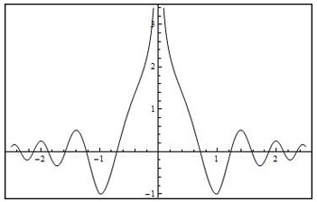
(a) real part graph of $u(t)$

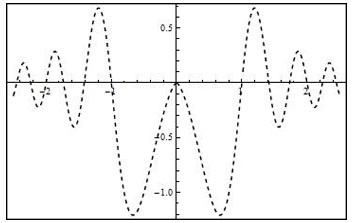
(b) imaginary part graph of $u(t)$

Figure 6.1: real and imaginary part graphs of $u(t)$ in time domain.

Consider the FRFT of $u$ of order $\pi/4$:

$$(\mathcal{F}_{\pi/4}u)(w)=2e^{i\pi w^{2}}\left(\frac{\text{C}\left(2^{5/4}\sqrt{\left|w\right|}\right)}{2^{1/4}\sqrt{\left|w\right|}}-\sqrt{2}\pi^{2}\left|w\right|+2\sqrt{2}\pi w\operatorname{Si}\left(2\sqrt{2}\pi w\right)+\cos\left(2\sqrt{2}\pi w\right)\right),$$

where $\operatorname{C}(x)$ and $\operatorname{Si}(x)$ denote the Fresnel integral and sine integral, respectively. Namely,

$$\text{C}(x) = \int_{0}^{x}\sin t^{2}\text{d}t=\sum\limits_{n=0}^{\infty}(-1)^{n}\frac{x^{4n+1}}{(2n)!(4n+1)},$$

$$\operatorname{Si}(x) = \int_{0}^{x}\frac{\sin t}{t}\text{d}t=\sum\limits_{n=0}^{\infty}(-1)^{n}\frac{x^{2n+1}}{(2n+1)!(2n+1)}.$$

The real and imaginary part graphs of $(\mathcal{F}_{\pi/4}u)(w)$ in frequency domain are shown in Fig 6.2.

(a) real part graph of $(\mathcal{F}_{\pi/4}u)(w)$

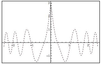
(b) imaginary part graph of $(\mathcal{F}_{\pi/4}u)(w)$

Figure 6.2: real and imaginary part graphs of $(\mathcal{F}_{\pi/4}u)(w)$ in frequency domain.

It is obvious that $\mathcal{F}_{\pi/4}u\notin L^{1}(\mathbb{R})$. The inverse FRFT

$$\int_{-\infty}^{+\infty}(\mathcal{F}_{\pi/4}u)(w)K_{-\pi/4}(x,t)\mathrm{d}w$$ (6.1)

do not make sense. In order to recover the original signal $u(t)$, we should use the approximating method. Fig. 6.3 shows the Abel means of the integral (6.1) with $\varepsilon=1,0.1,0.01$, that is,

$$u_{\varepsilon}(t)=\int_{-\infty}^{+\infty}(\mathcal{F}_{\pi/4}u)(w)K_{-\pi/4}(x,t)e^{-2\pi\varepsilon\left|\csc\alpha\right|\left|w\right|}\mathrm{d}w.$$

By Theorems 3.11-3.12 and Corollary 3.13 we know that $u_{\varepsilon}(t)\rightarrow u(t)$ for a.e. $t\in\mathbb{R}$ as $\varepsilon\rightarrow 0$.

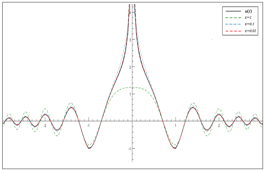
(a) real part graph of $u_{\varepsilon}(t)$

(b) imaginary part graph of $u_{\varepsilon}(t)$

Figure 6.3: real and imaginary part graphs of $u_{\varepsilon}(t)$