Asymptotic control of FWER under Gaussian assumption: application to correlation tests

Abstract

In many applications, hypothesis testing is based on an asymptotic distribution of statistics. The aim of this paper is to clarify and extend multiple correction procedures when the statistics are asymptotically Gaussian. We propose a unified framework to prove their asymptotic behavior which is valid in the case of highly correlated tests. We focus on correlation tests where several test statistics are proposed. All these multiple testing procedures on correlations are shown to control FWER. An extensive simulation study on correlation-based graph estimation highlights finite sample behavior, independence on the sparsity of graphs and dependence on the values of correlations. Empirical evaluation of power provides comparisons of the proposed methods. Finally validation of our procedures is proposed on real dataset of rats brain connectivity measured by fMRI. We confirm our theoretical findings by applying our procedures on a full null hypotheses with data from dead rats. Data on alive rats show the performance of the proposed procedures to correctly identify brain connectivity graphs with controlled errors.

Keywords. Multiple testing, structure learning, correlation tests, FWER control, cerebral connectivity

Consider a family of probability distributions $\mathcal{P}$. Let $\mathbb{X}^{(n)}=\left(X_{1},\dots,X_{n}\right)$ be independent realizations from an unknown probability distribution $P$. We assume that $P$ belongs to the family $\mathcal{P}$. Denote $\theta(P)=\big{(}\theta_{1}(P),\dots,\theta_{m}(P)\big{)}$ the parameter vector of interest, with $m\geq 2$. Observing $\mathbb{X}^{(n)}$, we aim at testing the following two-sided null hypotheses, for all $i\in\{1,\ldots,m\}$

$$H_{0,i}:\>\theta_{i}=0\text{\leavevmode\nobreak\ against \leavevmode\nobreak\ }H_{1,i}:\>\theta_{i}\neq 0.$$ (P-1)

For all $i\in\{1,\dots,m\}$, we consider test statistics $T_{n,i}\left(\mathbb{X}^{(n)}\right)$ chosen according to (P-1).

The objective of multiple testing procedure is to give a rejection set

$$\mathcal{R}=\{i,\;1\leq i\leq m:(H_{0,i})\text{\leavevmode\nobreak\ rejected}\},$$

such that the error is controlled. We will consider here the type I error called Family Wise Error Rate (FWER), defined as

$$\text{FWER}(\mathcal{R},P)=\mathbb{P}\left(\exists i\in\mathcal{R}:\theta_{i}=0\right).$$

To control the FWER for a given level $\alpha\in[0,1]$, the objective is to find a procedure yielding a rejection set $\mathcal{R}$ such that $\text{FWER}(\mathcal{R},P)\leq\alpha$.

The classical method to control the FWER is the Bonferroni, (1935)’s method where each individual hypothesis is tested at a significance level of $\alpha/m$ with $\alpha$ the desired overall FWER level and $m$ the total number of hypotheses to test. Although this method is very intuitive, it could be conservative if there is a large number of false hypotheses relative to the number of hypotheses being tested. Alternative methods have been proposed to improve the power, e.g. Holm, (1979), Dudoit et al., (2003), ponderated Bonferroni in Finner and Gontscharuk, (2009). Goeman and Solari, (2010) proposed a general framework to describe most of these methods by using the sequential rejection principle.

This manuscript investigates the problem of FWER control when the test statistics $T_{n,i}\left(\mathbb{X}^{(n)}\right)$ are possibly dependent and have an asymptotic Gaussian distribution. This work is motivated by an application in neuroscience (Achard et al.,, 2006). Let $V$ denote the set of the indexes of brain regions, $V=\{1,\dots,p\}$. Using brain imagery facilities, it is possible to record non invasively the activity of each brain regions. The data are then processed to give estimations of a correlation matrix between the activity of brain regions $(\rho_{i,j})_{(i,j)\in V\times V}$. The objective is to infer the dependence graph $G=(V,E)$ where the set of edges $E$ is a subset of $V\times V$ defined by $E=\{(i,j):\rho_{i,j}\neq 0\}.$ To estimate these edges, one has to consider for all $(i,j)\in V\times V$ the tests of the form

$$H_{0,ij}:\rho_{ij}=0\text{\leavevmode\nobreak\ against \leavevmode\nobreak\ }H_{1,ij}:\rho_{ij}\neq 0$$ (P-2)

where $\rho_{ij}$ denotes a correlation between a variable $i$ and a variable $j$, corresponding to nodes $V$. In this setting, test statistics $T_{n,ij}\left(\mathbb{X}^{(n)}\right)$ are asymptotically Gaussian and possibly highly correlated. We hence propose to apply a multiple testing procedure on correlations. The set of edges is then estimated as $\{(i,j)\in V\times V\;|\;H_{0,ij}\text{\leavevmode\nobreak\ is rejected}\}$. For a given graph $G$, estimation $\widehat{G}$ is obtained applying $m=p\,(p-1)/2$ tests (since the set $E$ is symmetric by symmetry of the correlations – the edges are undirected). Such an approach for graph inference has been proposed in Drton and Perlman, (2007). Other methods to estimate dependence graphs exist based on regularisation estimators (Friedman et al.,, 2008, Meinshausen and Bühlmann,, 2006). However, these methods need sparse assumptions on the graphs to be valid. In addition, to our knowledge, none of these latter methods ensures the control of FWER (Rothman et al.,, 2008, Krämer et al.,, 2009, Cai et al.,, 2011). As an example, simulation studies state that Graphical Lasso approach select too many edges, see e.g. Krämer et al., (2009). In applications such as network inference in neuroscience, a fine control of false discovered edges is crucial and this motivates the present work.

In this article, four existing asymptotic FWER controlling procedures are presented in an unified framework: Bonferroni, (1935), Dudoit et al., (2003), Romano and Wolf, (2005), Drton and Perlman, (2007). For each of them, we confirm that they control asymptotically the FWER for any underlying dependence structure, and when the sample size is sufficiently large. Recent results are reviewed in a more general setting. Our main contribution is to clarify and supplement existing results in the literature. Additionally we provide an extensive comparison of methods, with different statistics. An empirical evaluation of the power of the proposed method using different graph structures is described where it is shown that the sample size is the only crucial parameter. These results are then applied on a real dataset consisting of small animal brain recordings by fMRI, where recordings on dead rats provide a null model from the experiments Becq et al., 2020b .

The article is organized in five parts. The first part defines the asymptotic tests setting and describe the four multiple testing procedures. For each of these methods, single-step and step-down approaches are described. The second part is dedicated to the application to multiple correlation testing. Simulations are proposed in a third part, where we study among others the behavior of the power with respect to the sparsity of the set of rejected hypothesis. In the fourth part, our approach is applied to a real fMRI dataset on rats. Finally, we comment a possible extension to False Discovery Rate control.

1 Procedures controlling asymptotically the FWER

For all $i\in\{1,\ldots,m\}$, we consider tests (P-1), based on test statistics $T_{n,i}\left(\mathbb{X}^{(n)}\right)$. Fix $T_{n,i}\left(\mathbb{X}^{(n)}\right)=\sqrt{n}\>\widehat{\theta}_{n,i}\left(\mathbb{X}^{(n)}\right).$ Throughout this manuscript, we assume that $\widehat{\theta}_{n,\cdot}\left(\mathbb{X}^{(n)}\right)$ is a consistent estimator of $\theta(P)$ and that it has an asymptotic Gaussian distribution. Namely, for all $P\in\mathcal{P}$

$$\sqrt{n}\left(\>\widehat{\theta}_{n,\cdot}(\mathbb{X}^{(n)})-\theta(P)\right)\mathop{\longrightarrow}^{\quad d\quad}\mathcal{N}_{m}(0,\Sigma),\quad\text{when\leavevmode\nobreak\ }{n\to+\infty},$$ (1)

where $\displaystyle{\mathop{\longrightarrow}^{\quad d\quad}}$ denotes the convergence in distribution. We assume that $\Sigma$ is invertible and $\Sigma_{ii}=1$ when $\theta_{i}=0$. That is, every statistic is normalized under the null hypothesis of (P-1), so that $\mbox{Var}(T_{i})=1$, for all $i\in\{j:H_{0j}\text{\leavevmode\nobreak\ holds}\}$. It is not restrictive since one needs to control the variance of the statistics independently of the observations in order to apply a statistical test.

Let $\left(p_{n,i}\left(\mathbb{X}^{(n)}\right)\right)_{1\leq i\leq m}$ be a family of $p$-values resulting from each $m$ individual test. The asymptotic Gaussian assumption (1) gives rise to the asymptotic $p$-value process:

$$\forall i\in\{1,\ldots,m\},\>p_{n,i}\left(\mathbb{X}^{(n)}\right)=2\left[1-\Phi\left(\bigl{|}T_{n,i}(\mathbb{X}^{(n)})\bigr{|}\right)\right],$$ (2)

where $\Phi$ is the standard Gaussian cumulative distributive function. Multiple testing procedures will be based on this $p$-value process. It is worth pointing that no assumption on the dependence structure of the $p$-values is needed.

In this section, we proceed with the study of testing simultaneously $m$ hypotheses, $H_{0,i}$ against $H_{1,i}$ for $i\in\{1,\dots,m\}$. Results are reviewed in a more general setting where the Family Wise Error Rate (FWER) is used as multiple testing criterion.

For all $P\in\mathcal{P}$, let $\mathcal{H}_{0}(P)=\{i\in\{1,\ldots,m\}:\theta_{i}=0\}$ be the index set of true null hypotheses, that is, the index set of all $i$ such that $H_{0,i}$ is satisfied for $P$. Denote $m_{0}(P)=|\mathcal{H}_{0}(P)|$, its cardinality. The FWER depends on the rejected set $\mathcal{R}$ and on the (unknown) distribution $P$ of the observations. The FWER corresponds to the probability of rejecting at least one true null hypothesis, namely

$$\forall P\in\mathcal{P},\text{ FWER}(\mathcal{R},P)=\mathbb{P}(|\mathcal{R}\cap\mathcal{H}_{0}(P)|\geq 1).$$ (3)

Since we consider an asymptotic $p$-value process, we can only get asymptotic results in terms of control of the errors.

Definition 1.1.

A multiple testing procedure $\mathcal{R}$ is said to asymptotically control the FWER for a distribution family $\mathcal{P}$ at level $\alpha$ if for all $P\in\mathcal{P}$,

$$\underset{n\to+\infty}{\limsup}\text{ FWER}(\mathcal{R},P)\leq\alpha.$$ (4)

In this section we will describe multiple testing procedures which asymptotically control FWER for the two-sided testing problem (P-1), based on the asymptotic $p$-value process (2).

1.1 Single-step procedures

We propose four procedures to determine the rejection set.

Bonferroni

The Bonferroni procedure, Bonferroni, (1935), is the most classical example of FWER control.

Method 1 (Bonferroni).

The Bonferroni multiple testing procedure is defined by

$$\mathcal{R}^{bonf}_{\alpha}=\left\{i\in\{1,\ldots,m\}:p_{n,i}\leq\frac{\alpha}{m}\right\}.$$ (5)

Proposition 1.1.

For the two-sided testing problem (P-1) based on the asymptotic $p$-value process (2), the method $\mathcal{R}^{bonf}_{\alpha}$ provides an asymptotic control of the FWER at level $\alpha$, that is, for all $P\in\mathcal{P}$,

$$\underset{n\to+\infty}{\lim}\rm{FWER}\Big{(}\mathcal{R}^{bonf}_{\alpha},P\Big{)}\leq\alpha.$$

This control does not require any assumption on the dependence structure of the $p$-values, however under strong dependence the Bonferroni correction is known to be conservative, see Bland and Altman, (1995).

Šidák

As mentioned by Westfall and Young, (1993), an asymptotic FWER controlling procedure can be derived by Šidák’s inequality (Šidák,, 1967).

Theorem 1.1 (Šidák’s inequality, Šidák, (1967)).

Let $X$ be a random vector having an $m$-multivariate normal distribution with zero mean values and invertible covariance matrix. Then $X$ satisfies the following inequality, for every positive constant $b\in\mathbb{R}^{m}_{+}$,

$$\mathbb{P}(|X_{1}|\leq b_{1},\ldots,|X_{m}|\leq b_{m})\,\geq\,\prod_{i=1}^{m}\mathbb{P}(|X_{i}|\leq b_{i}).$$ (6)

For the specific case of correlation testing, Drton and Perlman, (2004) used this inequality to construct a procedure that asymptotically controls the FWER for the problem (P-1).

Method 2 (Šidák).

Let $c_{\alpha}^{s}=\Phi^{-1}\Big{(}\frac{1}{2}(1-\alpha)^{1/m}+\frac{1}{2}\Big{)}>0$. The Šidák’s multiple testing procedure is defined by

$$\mathcal{R}^{s}_{\alpha}=\big{\{}i\in\{1,\ldots,m\}:|T_{n,i}|>c_{\alpha}^{s}\big{\}}.$$ (7)

Proposition 1.2.

For the two-sided testing problem (P-1) for which the asymptotic Gaussian assumption (1) holds, the method $\mathcal{R}^{s}_{\alpha}$ provides an asymptotic control of the FWER at level $\alpha$, namely, for all $P$ such that $\Sigma$ is invertible,

$$\underset{n\to+\infty}{\lim}\>\rm{FWER}(\mathcal{R}^{s}_{\alpha},P)\leq\alpha.$$

The procedure is valid for any dependencies, as soon as the inequality (6) holds. This is in particular true in Gaussian setting (Šidák,, 1967).

The Šidák’s procedure is less conservative than the Bonferroni procedure. This comparison is illustrated in table 2.2 of Westfall and Young, (1993), where the difference between the two adjustments becomes larger with larger $m$.

Non parametric bootstrap

Romano and Wolf, (2005) propose an asymptotic FWER controlling procedure which only requires a monotonic assumption on the family of thresholds.

Method 3 (BootRW).

For all $\mathcal{C}\subset\{1,\ldots,m\}$, let $t_{n,\alpha}(\Sigma,\mathcal{C})$ be the $(1-\alpha)$-quantile of the probability distribution $\mathcal{L}\left(\|\left.\mathcal{N}_{m}(0,\Sigma)\right\lvert_{\mathcal{C}}\|_{\infty}\right)$, where $\left.\mathcal{N}_{m}(0,\Sigma)\right\lvert_{\mathcal{C}}$ is the restriction of the Gaussian distribution $\mathcal{N}_{m}(0,\Sigma)$ on $\mathcal{C}$, namely $\mathcal{N}_{|\mathcal{C}|}\Big{(}0,(\Sigma)_{i,i^{\prime}\in\mathcal{C}\times\mathcal{C}}\Big{)}$. The Romano-Wolf’s multiple testing procedure is defined by

$$\mathcal{R}^{BootRW}_{\alpha}=\Big{\{}i\in\{1,\ldots,m\}:|T_{n,i}|>\widehat{t}_{n,\alpha}(\Sigma,\mathcal{C}_{m})\Big{\}},$$ (8)

where $\mathcal{C}_{m}=\{1,\ldots,m\}$ and $\widehat{t}_{n,\alpha}(\Sigma,\mathcal{C}_{m})$ is computed using bootstrap resamples of $\mathbb{X}^{(n)}$. A bootstrap resample from $\mathbb{X}^{(n)}$ is denoted by $\mathbb{X}^{(n)^{*}}$ and defined as an $n$ independent and identically distributed (i.i.d.) sample from the empirical distribution of $\mathbb{X}^{(n)}$.

Note that this method closely relies on its ability to approximate the joint distribution of the test statistics.

Proposition 1.3 (Romano and Wolf, (2005)).

Assume that for any metric $d$ metrizing weak convergence on $\mathbb{R}^{m_{0}(P)}$,

$$d\left(\mathcal{L}\left(\left(T_{n,i}\left(\mathbb{X}^{(n)^{*}}\right)\right)_{i\in\mathcal{H}_{0}(P)}\Big{|}\>\mathbb{X}^{(n)}\right),\mathcal{L}\left(\left(T_{n,i}\left(\mathbb{X}^{(n)}\right)\right)_{i\in\mathcal{H}_{0}(P)}\right)\right)\overset{\mathbb{P}}{\longrightarrow}0,$$

where $\overset{\mathbb{P}}{\longrightarrow}$ means a convergence in probability. $\mathcal{L}\left(\left(T_{n,i}\left(\mathbb{X}^{(n)^{*}}\right)\right)_{i\in\mathcal{H}_{0}(P)}\Big{|}\>\mathbb{X}^{(n)}\right)$ denotes the conditional distribution of $\left(T_{n,i}\left(\mathbb{X}^{(n)^{*}}\right)\right)_{i\in\mathcal{H}_{0}(P)}$ given $\mathbb{X}^{(n)}$.

Then, for the two-sided testing problem (P-1) for which the asymptotic Gaussian assumption (1) holds, the method $\mathcal{R}^{BootRW}_{\alpha}$ provides an asymptotic control of the FWER at level $\alpha$, that is, for all $P$ such that $\Sigma$ is invertible,

$$\underset{n\to+\infty}{\limsup}\>\rm{FWER}(\mathcal{R}^{BootRW}_{\alpha},P)\leq\alpha.$$

This result is also derived in Dudoit and Van Der Laan, (2007) (where BootRW is procedure 4.21). The proof in our setting is rewritten in the Appendix.

Parametric bootstrap

Drton and Perlman, (2007) detailled a parametric bootstrap method for testing (P-1) on partial correlation coefficients. This method differs from Romano and Wolf, (2005). Indeed, the quantile is here evaluated on the asymptotic distribution rather than the empirical distribution. An estimation of the matrix $\Sigma$ is needed. Denote by $\widehat{\Sigma}_{n}$ such an estimator.

Method 4 (MaxT).

Let $t_{n,\alpha}(\widehat{\Sigma}_{n})$ be the $(1-\alpha)$-quantile of the distribution $\mathcal{L}\Big{(}\|\mathcal{N}_{m}(0,\widehat{\Sigma}_{n})\|_{\infty}\Big{)}$. The MaxT multiple testing procedure is defined by

$$\mathcal{R}^{MaxT}_{\alpha}=\Big{\{}i\in\{1,\ldots,m\}:|T_{n,i}|>t_{n,\alpha}\big{(}\widehat{\Sigma}_{n}\big{)}\Big{\}},$$ (9)

where $t_{n,\alpha}\big{(}\widehat{\Sigma}_{n}\big{)}$ is computed using (simulated) samples of $\mathcal{N}_{m}(0,\widehat{\Sigma}_{n})$.

Proposition 1.4.

Assume that $(\widehat{\Sigma}_{n})$ is a consistent estimator of $\Sigma$, that is, when $n$ goes to infinity,

$$\widehat{\Sigma}_{n}\overset{\mathbb{P}}{\longrightarrow}\Sigma.$$ (10)

Then, for the two-sided testing problem (P-1) for which the asymptotic Gaussian assumption (1) holds, the method $\mathcal{R}^{MaxT}_{\alpha}$ provides an asymptotic control of the FWER at level $\alpha$, namely, for all $P$ such that $\Sigma$ is invertible,

$$\underset{n\to+\infty}{\limsup}\>\rm{FWER}(\mathcal{R}^{MaxT}_{\alpha},P)\leq\alpha.$$ (11)

Even if many results are known on the maximum of Gaussian variables (see e.g. Nadarajah and Kotz, (2008) and references therein), there is no explicit formula of quantile $t_{n,\alpha}(\widehat{\Sigma}_{n})$ of absolute multivariate Gaussian distributions in general case. Therefore an estimation is required. We propose here to estimate the quantile by parametric bootstrap in Method 4. It is also possible to use, for example, Genz and Bretz, (2009)’s algorithm (available in function qmvnorm of mvtnorm on R). However, even if the estimation has a good quality, the computational cost is very high.

Procedure MaxT is available with any consistent estimation of $\Sigma$. However, in practice, the quality of estimation may influence the quality of the procedure for a given number $n$ of observations.

A natural candidate for $\widehat{\Sigma}_{n}$ is the empirical covariance of observations $\mathbb{X}^{(n)}$. Yet, Johnstone, (2001) established that when $n$ increases while $\frac{p}{n}$ converges to a constant, on zero limit, then the empirical estimation provides a non consistent estimate because its eigenvalues do not converge to those of the covariance matrix. Several methods have been proposed to reduce the dimension of the estimation setting to overpass this problem, requiring assumptions of sparsity or structured matrices. For examples, we can cite banding methods in Bickel and Levina, 2008b and Wu and Pourahmadi, (2009), thresholding rules in Bickel and Levina, 2008a for instance, shrinkage estimation in Ledoit et al., (2012) and convex optimization techniques in Banerjee et al., (2006). Those estimators can be plugged into MaxT procedure.

1.2 Step-down versions

Single-step methods can be conservative. A well-known improvement is step-down method. It is a recursive algorithm which increases the power of the procedures, still preserving FWER control. See e.g. Romano and Wolf, (2005), Goeman and Solari, (2010). The principle is to iterate multiple testing on the non-rejected hypothesis, as described below.

Step-down Algorithm.

  Let $\mathcal{C}_{0}=\varnothing$ and $\mathcal{C}_{1}=\{1,\ldots,m\};$

  Initialize $j=1$.

  while $\mathcal{C}_{j}\neq\mathcal{C}_{j-1}$ do

     Let $R_{j}$ be the set of rejected indexes of a given multiple testing procedure applied on tests indexes $\mathcal{C}_{j}$.

     Define ${\mathcal{C}}_{j+1}=\{i\in{\mathcal{C}}_{j},\;i\notin R_{j}\}$.

     Do $j=j+1$.

  end while

  return  ${\mathcal{C}}_{\infty}=\mathcal{C}_{j}.$

  ${\mathcal{C}}_{\infty}$ is the final set of non-rejected null-hypothesis indexes.

If a single-step method provides an asymptotic control of the FWER, then the following proposition provides sufficient conditions under which its step-down version preserves this control.

Proposition 1.5.

Let $\big{(}R_{\mathcal{C}}\big{)}_{\mathcal{C}\subset\mathcal{H}}$ be a family of rejection sets given by multiple testing procedure. Suppose that

• For all  $P\in\mathcal{P},$

  $$\underset{n\to+\infty}{\limsup}\text{ FWER}\Big{(}R_{\mathcal{H}_{0}(P)},P\Big{)}\leq\alpha,$$ (12)

• For all $\mathcal{C}\subset\{1,\ldots,m\},\>\mathcal{C}\mapsto\mathcal{R}_{\mathcal{C}}$ is decreasing in $\mathcal{C}$, that is,

  $$\forall\mathcal{C},\mathcal{C}^{\prime}\subseteq\{1,\ldots,m\},\mathcal{C}\subseteq\mathcal{C}^{\prime}\Rightarrow\mathcal{R}_{\mathcal{C}}\supseteq\mathcal{R}_{\mathcal{C}^{\prime}}.$$ (13)

Then, for all $P\in\mathcal{P}$,

$$\underset{n\to+\infty}{\limsup}\text{ FWER }\Big{(}R_{{\mathcal{C}}_{\infty}},P\Big{)}\leq\alpha.$$

We deduce that the four methods displayed above control asymptotically the FWER for tests (P-1).

Corrollary 1.1.

For the two-sided testing problem (P-1) for which the asymptotic Gaussian assumption (1) holds, step-down algorithm applied to Methods 1 to 4 are asymptotic FWER controlling procedures at level $\alpha$.

Proof.

It is sufficient to verify that the four methods satisfy (12) and (13). ∎

2 Application to correlation tests

Let $\left\{Y_{1},\ldots,Y_{n}\right\}$ be independent realizations from a random vector $Y$ with values in $\mathbb{R}^{p}$. Denote $Y=(Y^{(i)})_{i=1,\dots,p}$. Suppose $Y$ has a finite expectancy and a semi-definite positive covariance matrix. Assume also that $Y$ has finite fourth moments. Define $\Gamma=(\rho_{ij})_{i,j=1,\dots,p}$ the correlation matrix of $Y$. That is, $\rho_{ij}=\text{Cor}(Y^{(i)},Y^{(j)})$. Consider the two-sided testing problem:

$$H_{0,ij}:\rho_{ij}=0\text{\leavevmode\nobreak\ against \leavevmode\nobreak\ }H_{1,ij}:\rho_{ij}\neq 0,\quad(i,j)\in\mathcal{H},$$ (P-2)

where $\mathcal{H}$ is the set of tested indexes, $\mathcal{H}=\{1\leq i<j\leq p\}$. The $p$-value processes associated to tests (P-2) present a dependence structure which is possible to detail for different tests statistics.

Usual statistics proposed in literature for tests (P-2) are based on the empirical correlation. Define $\widehat{\rho_{ij}}=\frac{1}{n}\sum_{\ell=1}^{n}(Y^{(i)}_{\ell}-\overline{Y^{(i)}})(Y^{(j)}_{\ell}-\overline{Y^{(j)}})$, the empirical correlation between $\left\{Y_{1}^{(i)},\ldots,Y_{n}^{(i)}\right\}$ and $\left\{Y_{1}^{(j)},\ldots,Y_{n}^{(j)}\right\}$, for $i,j=1,\dots,p$. The overline denotes the empirical mean, that is, $\overline{Y^{(i)}}=\frac{1}{n}\sum_{\ell=1}^{n}Y_{\ell}^{(i)}$. Denote $\widehat{\Gamma}_{n}=(\widehat{\rho}_{ij})_{1\leq i,j\leq p}$. We will focus our analysis on four test statistics:

Empirical statistic.

$$T^{(1)}(\widehat{\rho}_{ij})=\sqrt{n}\,\widehat{\rho}_{ij}$$

Student statistic.

$$T^{(2)}(\widehat{\rho}_{ij})=\sqrt{n-2}\,\frac{\widehat{\rho}_{ij}}{\sqrt{1-\widehat{\rho}_{ij}^{2}}}$$

See e.g. Section 4.2.1 of Anderson, (2003).

Fisher statistic.

$$T^{(3)}(\widehat{\rho}_{ij})=\frac{\sqrt{n-3}}{2}\log\left(\frac{1+\widehat{\rho}_{ij}}{1-\widehat{\rho}_{ij}}\right)\,.$$

Fisher transform is commonly used to improve the convergence to the Gaussian distribution for univariate statistics (i.e. for fixed $(i,j)$) (see Section 4.2.3 of Anderson, (2003)).

Second-order statistic.

For given $(i,j)\in\mathcal{H}$ such that $\mbox{Var}(Y^{(i)})=\mbox{Var}(Y^{(j)})=1$, $\widehat{\rho}_{ij}$ is the empirical mean of $(Z_{\ell}^{(ij)})_{\ell=1,\dots,n}$ with $Z_{\ell}^{(ij)}=(Y_{\ell}^{(i)}-\overline{Y^{(i)}})(Y^{(j)}_{\ell}-\overline{Y^{(j)}})$. Hence a test on $\widehat{\rho}_{ij}$ can be driven using the usual test statistics on an expectation under asymptotic Gaussian assumption:

$$T^{(4)}_{ij}=\sqrt{n}\,\frac{\overline{Z^{(ij)}}}{\sqrt{\widehat{\theta}_{ij}}}\text{\leavevmode\nobreak\ where\leavevmode\nobreak\ }\widehat{\theta}_{ij} =\frac{1}{n}\sum_{\ell=1}^{n}\left(Z^{(ij)}_{\ell}-\frac{1}{n}\sum_{\ell^{\prime}=1}^{n}Z^{(ij)}_{\ell^{\prime}}\right)^{2}\,.$$

The quantity $\widehat{\theta}_{ij}$ is an estimation of

$$\theta_{ij}=\mbox{Var}\left[(Y^{(i)}-\mathbb{E}(Y^{(i)}))(Y^{(j)}-\mathbb{E}(Y^{(j)}))\right].$$

When $(i,j)\in\mathcal{H}_{0}$, $\mathbb{E}(T^{(4)}_{ij})=0$. Cai and Liu, (2016) studied these statistics for multiple testing of correlations.

Asymptotics of the empirical correlations are derived in Aitkin, (1969) where the author established the asymptotic normality for Gaussian distributed $Y$, and in Steiger and Hakstian, (1982) for non Gaussian distribution.

Proposition 2.1 (Aitkin, (1969), Steiger and Hakstian, (1982)).

Let $\left\{Y_{1},\ldots,Y_{n}\right\}$ be independent realizations from a random vector $Y=(Y^{(i)})_{i=1,\dots,p}$. Suppose $Y$ has finite fourth moments.

The vector of empirical correlations $\widehat{\rho}_{n,\cdot}=(\widehat{\rho}_{n,h})_{h\in\mathcal{H}}$ is asymptotically Gaussian,

$$\sqrt{n}(\widehat{\rho}_{n,\cdot}-\rho_{\cdot})\xrightarrow[n\to+\infty]{\quad d\quad}\mathcal{N}_{m}(0,\Omega(\Gamma)),$$

with $\Omega(\Gamma)=(\omega_{ij,kl})_{(ij,kl)\in\mathcal{H}^{2}}$ given by

$$\omega_{ij,kl}=\rho_{ijkl}+\frac{1}{4}\rho_{ij}\rho_{kl}\Big{(}\rho_{iikk}+\rho_{iill}+\rho_{jjkk}+\rho_{jjll}\Big{)}\\ -\frac{1}{2}\rho_{ij}\Big{(}\rho_{iikl}+\rho_{jjkl}\Big{)}-\frac{1}{2}\rho_{kl}\Big{(}\rho_{ijkk}+\rho_{ijll}\Big{)},$$

where for all $i,j,k,l$,

$$\rho_{ijkl}=\frac{\mathbb{E}\left[(Y^{(i)}-\mathbb{E}(Y^{(i)}))(Y^{(j)}-\mathbb{E}(Y^{(j)}))(Y^{(k)}-\mathbb{E}(Y^{(k)}))(Y^{(l)}-\mathbb{E}(Y^{(l)}))\right]}{\sqrt{\mathrm{Var}(Y^{(i)})\mathrm{Var}(Y^{(j)})\mathrm{Var}(Y^{(k)})\mathrm{Var}(Y^{(l)})}}.$$

In particular, when $Y$ is Gaussian, $\Omega(\Gamma)=(\omega_{ij,kl})_{(ij,kl)\in\mathcal{H}^{2}}$ satisfies

$$\omega_{ij,ij} =\Big{(}1-\rho_{ij}^{2}\Big{)}^{2},$$

$$\omega_{ij,il} =-\frac{1}{2}\rho_{ij}\rho_{il}\Big{(}1-\rho_{ij}^{2}-\rho_{il}^{2}-\rho_{jl}^{2}\Big{)}+\rho_{jl}\Big{(}1-\rho_{ij}^{2}-\rho_{il}^{2}\Big{)},\quad\text{for\leavevmode\nobreak\ }j\neq l$$

$$\omega_{ij,kl} =\frac{1}{2}\rho_{ij}\rho_{kl}\Big{(}\rho_{ik}^{2}+\rho_{il}^{2}+\rho_{jk}^{2}+\rho_{jl}^{2}\Big{)}+\rho_{ik}\rho_{jl}+\rho_{il}\rho_{jk}$$

$$\qquad-\rho_{ik}\rho_{jk}\rho_{kl}-\rho_{ij}\rho_{ik}\rho_{il}-\rho_{ij}\rho_{jk}\rho_{jl}-\rho_{il}\rho_{jl}\rho_{kl},\quad\text{for\leavevmode\nobreak\ }i\neq k\text{\leavevmode\nobreak\ and\leavevmode\nobreak\ }j\neq l.$$

Asymptotic distributions of test statistics $\{(T_{ij}^{(k)})_{1\leq i<j\leq n},k=1,\dots,4\}$ follow.

Corrollary 2.1.

For all $k=1,\dots,3$, vector statistics $(T^{(k)}(\widehat{\rho}_{ij}))_{1\leq i<j\leq p}$ converge in distribution to a Gaussian random variable with covariance matrix $\Omega^{(k)}(\Gamma)$,

$$(T^{(k)}(\widehat{\rho}_{ij})-T^{(k)}(\rho_{ij}))_{1\leq i<j\leq p}\mathop{\longrightarrow}^{\quad d\quad}\mathcal{N}_{m}(0,\Omega^{(k)}(\Gamma)),\quad\text{when\leavevmode\nobreak\ }{n\to+\infty},$$

where

• $\Omega^{(1)}(\Gamma)=\Omega(\Gamma)$ defined in Proposition 2.1,

• $\Omega^{(2)}(\Gamma)=(\omega_{ij,kl}^{(2)})$ with $\omega_{ij,kl}^{(2)}=\omega_{ij,kl}/\left((1-\rho_{ij}^{2})(1-\rho_{kl}^{2})\right)^{3/2}$,

• $\Omega^{(3)}(\Gamma)=(\omega_{ij,kl}^{(3)})$ with $\omega_{ij,kl}^{(3)}=\omega_{ij,kl}/\left({(1-\rho_{ij}^{2})(1-\rho_{kl}^{2})}\right)$.

Proof.

Expressions of $\Omega^{(2)}(\Gamma)$ and $\Omega^{(3)}(\Gamma)$ result from the Delta method (Wasserman,, 2013). ∎

We can now state an equivalent result for Second-order statistics.

Proposition 2.2.

Let $\left\{Y_{1},\ldots,Y_{n}\right\}$ be independent realizations from a random vector $Y=(Y^{(i)})_{i=1,\dots,p}$. Suppose $Y$ has finite fourth moments.

Vector statistics $(T^{(4)}_{ij})_{1\leq i<j\leq p}$ converge in distribution to a Gaussian random variable with covariance matrix $\Omega^{(4)}(\Gamma)$,

$$(T^{(4)}_{ij}-\mathbb{E}(T^{(4)}_{ij}))_{1\leq i<j\leq p}\mathop{\longrightarrow}^{\quad d\quad}\mathcal{N}_{m}(0,\Omega^{(4)}(\Gamma)),\quad\text{when\leavevmode\nobreak\ }{n\to+\infty},$$

where $\Omega^{(4)}(\Gamma)=(\omega_{ij,kl}^{(4)})$ with $\omega_{ij,kl}^{(4)}=\rho_{ijkl}/\left({(\rho_{ijij}-\rho_{ij}^{2})(\rho_{klkl}-\rho_{kl}^{2})}\right)^{1/2}$.

When $Y$ is Gaussian, $\Omega^{(4)}(\Gamma)$ satisfies

$$\omega_{ij,kl}^{(4)}=\frac{\rho_{ij}\rho_{kl}+\rho_{ik}\rho_{jl}+\rho_{il}\rho_{kj}}{\left({(1+\rho_{ij}^{2})(1+\rho_{kl}^{2})}\right)^{1/2}}.$$

In particular, for all $(i,j)\in\mathcal{H}$, $\omega^{(4)}_{ij,ij}=1$.

Proof.

First, the law of large number ensures that for all $(i,j)\in\mathcal{H}$, $\widehat{\theta}_{ij}$ converges almost surely to $\theta_{ij}$. Applying Slutsky’s Theorem (Gut, (2012), Theorem 11.4) gives the asymptotic distribution of$\sqrt{n}\frac{\overline{Z^{(i,j)}}}{\widehat{\theta}_{ij}}$. Applying the continuity theorem on the characteristic functions, we deduce that the asymptotic distribution is Gaussian. The expression of $\Omega^{(4)}$ then results from the fact that $\theta_{ij}=(\rho_{ijij}-\rho_{ij}^{2})\sqrt{\mbox{Var}(Y_{i})\mbox{Var}(Y_{j})}$ and that $\mathbb{E}(Z^{(ij)}Z^{(kl)})=\rho_{ijkl}\sqrt{\mbox{Var}(Y_{i})\mbox{Var}(Y_{j})\mbox{Var}(Y_{k})\mbox{Var}(Y_{l})}$. ∎

To conclude, by Corollary 2.1, procedures of Section 1 can be applied. Single-step and step-down Methods 1–4 thus control asymptotically FWER. Methods 1–3 are non parametric, while Method 4 requires an explicit formula of the asymptotic covariance of tests statistics. In particular, the matrix $\Sigma$ in this method corresponds to $\Omega^{(k)}(\Gamma)$ given in Corollary 2.1 and Proposition 2.2. Method 4, MaxT, can then be applied by estimating quantiles using plug-in estimate of $\Omega^{(k)}(\Gamma)$. This consists simply in plugging in $\widehat{\Gamma}_{n}$ for $\Gamma$, where $\widehat{\Gamma}_{n}$ is an estimator of $\Gamma$. In the general case, such estimators need finite eight moments.

When the correlations are evaluated on Gaussian-distributed samples, for all $k=1,\dots,4$, matrices $\Omega^{(k)}(\Gamma)$ are explicitly given with respect to the correlation matrix $\Gamma$. Matrices $\Omega^{(k)}(\Gamma)$ can thus be estimated by $\Omega^{(k)}(\widehat{\Gamma}_{n})$, where $\widehat{\Gamma}_{n}$ is an estimator of $\Gamma$. In the following, we will consider that $\widehat{\Gamma}_{n}$ is the empirical correlation matrix. As previously, it is worth noticing that other estimators may have better performances. Obviously, it is possible to plug-in a matrix obtained e.g. by shrinkage estimation, banding methods, thresholding rules…

We can now state an adaptation of Method 4.

Method 4’ (MaxT for correlation tests (P-2)).

Assume $Y$ is Gaussian. Consider $k=1,\dots,4$. Let $t_{n,\alpha}(\widehat{\Sigma}^{(k)}_{n})$ be the $(1-\alpha)$-quantile of the distribution $\mathcal{L}\Big{(}\|\mathcal{N}_{m}(0,\widehat{\Sigma}^{(k)}_{n})\|_{\infty}\Big{)}$, with $\widehat{\Sigma}^{(k)}_{n}=\Omega^{(k)}(\widehat{\Gamma}_{n})$. The MaxT  multiple testing procedure is defined by

$$\mathcal{R}^{MaxT}_{\alpha}=\Big{\{}(i,j)\in\mathcal{H}:|T^{(k)}(\widehat{\rho}_{ij})|>t_{n,\alpha}^{(k)}\big{(}\widehat{\Sigma}^{(k)}\big{)}\Big{\}},$$ (14)

where $t_{n,\alpha}^{(k)}\big{(}\widehat{\Sigma}^{(k)}_{n}\big{)}$ is computed using (simulated) samples of $\mathcal{N}_{m}(0,\widehat{\Sigma}^{(k)}_{n})$.

Lemma 2.1 below then ensures that Method 4’ controls asymptotically FWER.

Lemma 2.1.

Assume $Y$ is Gaussian. For $k=1,\dots,4$, $\Omega^{(k)}(\widehat{\Gamma}_{n})$ tends in probability to $\Omega^{(k)}(\Gamma)$ when $n$ goes to infinity.

Proof.

Proposition 2.1 ensures that $\sqrt{n}(\widehat{\Gamma}_{n}-\Gamma)\xrightarrow[n\to+\infty]{\quad d\quad}\mathcal{N}_{m}(0,\Omega(\Gamma))$. Since $\frac{1}{\sqrt{n}}\xrightarrow[n\to+\infty]{\quad\mathbb{P}\quad}0$, Slutsky’s theorem (Gut, (2012), Theorem 11.4) implies that $\widehat{\Gamma}_{n}-\Gamma\overset{\mathbb{P}}{\longrightarrow}0$, that is, $\widehat{\Gamma}_{n}\overset{\mathbb{P}}{\longrightarrow}\Gamma$ when $n$ goes to infinity. We conclude using the continuous mapping Theorem (Gut, (2012), Theorem 10.3). ∎

Remark that all our results can be extended immediately to multiple testing of partial correlation (see Roux, (2018), Section 5.2.4). Indeed, similar convergence as in Proposition 2.1 exists for partial correlation (Aitkin,, 1969). Statistics in Methods 1-4 can be rewritten using partial correlation and asymptotic normality also holds.

3 Simulations

Correlation matrices can be used to define adjacency matrices of dependence graphs, where nodes correspond to variables and edges correspond to non zero of adjacency matrices (see e.g. Drton and Perlman, (2007)). In practice, empirical correlations are often full matrices, while dependence graphs are expected to have a smaller set of edges, see e.g. Kolaczyk, (2009), Newman, (2010). Thus multiple testing on correlations can be used for a better graph estimation, where only significant correlations $\rho_{ij}$ give an edge between nodes $i$ and $j$. A prior in many graph estimations is the sparsity of the estimated graph, e.g. in Graphical Lasso, Friedman et al., (2008). However, this crucial point may not be satisfied in real data applications, for instance in neuroscience (Markov et al.,, 2013).

Simulations are conducted to evaluate the behavior of the proposed approaches described in previous parts 1 and 2. Indeed, we showed that the FWER is controlled asymptotically and that the choice of the statistics may influence the asymptotic control. We conduct a precise and careful evaluation of the proposed methods by computing the number of falsely detected edges (FWER) and correctly identified edges (power – also named sensitivity). Three main parameters of the methods are varied: sparsity of the true graphs, size of the sample, and signal to noise ratio. After presenting the graph model chosen in our simulations, the results are displayed for FWER and latter for power.

Simulations were done on R with igraph and TestCor packages, Csardi and Nepusz, (2006), Gannaz, (2019).

3.1 Choice of models

Our simulation procedure requires the simulation of Gaussian data with a given covariance matrix defined in order to match a given graph structure. In addition, the covariance matrix has to be positive definite. It is rather simple to get an adjacency matrix following a network model such as small-world or scale-free (Newman,, 2010). However, it is difficult to guarantee its positive definiteness theoretically, see Guillot and Rajaratnam, (2012). Starting from a network model, we propose to generate a corresponding adjacency matrix, denoted $\mathbf{A}$. One way to guarantee the positive definiteness of the matrix is to control the eigenvalues. This is the purpose of the following lemma 3.1.

From the adjacency matrix $\mathbf{A}$ we build a correlation matrix $\mathbf{M}$ with a constant non zero value $\rho$ by

$$\mathbf{M}=\mathbf{I}+\rho\mathbf{A},$$

where $\mathbf{I}$ is the identity matrix, and $\rho\in(-1,1)$.

Lemma 3.1.

Let $\mathbf{M}$ satisfy $\mathbf{M}=\mathbf{I}+\rho\mathbf{A}$ with $\rho$ a real. Then, $\mathbf{M}$ is positive definite if and only if $|\rho|<\frac{1}{|\lambda_{min}|}$, where $\lambda_{min}$ is the smallest eigenvalue of $\mathbf{A}$.

For regular graphs, it is shown that $\lambda_{min}<-1/r$ independently on the size of the graph, where $r$ is the valence of the graph (Cvetkovic et al.,, 2004). In particular, for a chain graph, $|\rho|<0.5$ always gives a positive definite matrix $\mathbf{M}$. It is getting more complicated for small-world or scale-free models (Cvetkovic et al.,, 2004). A classical approach to ensure positive definiteness is diagonal dominance (see e.g. Schäfer and Strimmer, (2005) with precision matrices). Our model is quite similar, but considers constant non-zero entries in the correlation matrix.

In the sequel, we focus on Stochastic Block Models (Rohe et al.,, 2011). We consider a model where the number of nodes $p$ is equal to 26, with two community of size $p/2=13$. The adjacency matrix $\mathbf{A}$ is defined as

$$\mathbf{A}=\leavevmode\hbox to220.24pt{\vbox to241.76pt{\text{[drawing]}}} \left(\vbox{\hrule height=119.53215pt,depth=119.53215pt,width=0.0pt}\right. \left.\vbox{\hrule height=119.53215pt,depth=119.53215pt,width=0.0pt}\right) \bigl{(}a_{i,j}\bigr{)}_{\vbox{\Let@\restore@math@cr\default@tag\halign{\hfil$\m@th\scriptstyle#$&$\m@th\scriptstyle{}#$\hfil\cr i&=1,\dots,p/2\\ j&=1,\ldots,p/2\crcr}}} \bigl{(}b_{i,j}\bigr{)}_{\vbox{\Let@\restore@math@cr\default@tag\halign{\hfil$\m@th\scriptstyle#$&$\m@th\scriptstyle{}#$\hfil\cr i&=p/2+1,\dots,p\\ j&=1,\ldots,p/2\crcr}}} \bigl{(}a_{i,j}\bigr{)}_{\vbox{\Let@\restore@math@cr\default@tag\halign{\hfil$\m@th\scriptstyle#$&$\m@th\scriptstyle{}#$\hfil\cr i&=p/2+1,\dots,p\\ j&=p/2+1,\ldots,p\crcr}}} \bigl{(}b_{i,j}\bigr{)}_{\vbox{\Let@\restore@math@cr\default@tag\halign{\hfil$\m@th\scriptstyle#$&$\m@th\scriptstyle{}#$\hfil\cr i&=p/2+1,\dots,p\\ j&=1,\ldots,p/2\crcr}}} \left(\vbox{\hrule height=119.53215pt,depth=119.53215pt,width=0.0pt}\right. \left.\vbox{\hrule height=119.53215pt,depth=119.53215pt,width=0.0pt}\right) \bigl{(}a_{i,j}\bigr{)}_{\vbox{\Let@\restore@math@cr\default@tag\halign{\hfil$\m@th\scriptstyle#$&$\m@th\scriptstyle{}#$\hfil\cr i&=1,\dots,p/2\\ j&=1,\ldots,p/2\crcr}}} \bigl{(}b_{i,j}\bigr{)}_{\vbox{\Let@\restore@math@cr\default@tag\halign{\hfil$\m@th\scriptstyle#$&$\m@th\scriptstyle{}#$\hfil\cr i&=p/2+1,\dots,p\\ j&=1,\ldots,p/2\crcr}}} \bigl{(}a_{i,j}\bigr{)}_{\vbox{\Let@\restore@math@cr\default@tag\halign{\hfil$\m@th\scriptstyle#$&$\m@th\scriptstyle{}#$\hfil\cr i&=p/2+1,\dots,p\\ j&=p/2+1,\ldots,p\crcr}}} \bigl{(}b_{i,j}\bigr{)}_{\vbox{\Let@\restore@math@cr\default@tag\halign{\hfil$\m@th\scriptstyle#$&$\m@th\scriptstyle{}#$\hfil\cr i&=p/2+1,\dots,p\\ j&=1,\ldots,p/2\crcr}}}$$

where $(a_{i,j})_{i,j}$ are independent observations from a Bernoulli distribution with parameter $p_{intra}$ and $(b_{i,j})_{i,j}$ are independent observations from a Bernoulli distribution with parameter $p_{inter}$. In simulations, the probability to have an edge between nodes inside each communities is set to $p_{intra}=0.6$. Four values of the probability of connection between the two communities are considered, $p_{inter}\in\{0.01,0.05,0.15,0.4\}$. The corresponding adjacency matrices are displayed in Figure 1. Parameter $p_{inter}$ determines the degree of sparsity of the correlation matrix, where sparsity corresponds to the number of edges present in the graph with respect to the corresponding complete graph. High values of $p_{inter}$ means a low sparsity.

As explained above, we consider a constant value of non-zero correlations, $\rho$. The value must be chosen such that the resulting matrix $\mathbf{M}$ is positive definite. In our application, it implies that $\rho\leq 0.2$, independently of $p_{inter}$ and $p_{intra}$.

The choice of maximal value of $\rho$ is linked to the density of the graph. Indeed, the denser the graph is, the smaller $\rho$ has to be chosen. We choose the same values of $\rho$ here whatever the adjacency matrix is, to study more specifically the influence of the sparsity. As noticed e.g. by Krämer et al., (2009), the recovery of the edges is in general more difficult when the sparsity of the graph decreases. The authors also remarked that all methods perform well with cluster networks. This observation motivates the analysis of the behavior of multiple testing approaches with respect to the sparsity.

Figure 1: Adjacency matrices. The parameter $sparse$ is the proportion of edges present in the graph with respect to a complete graph. $p_{intra}=0.6$.

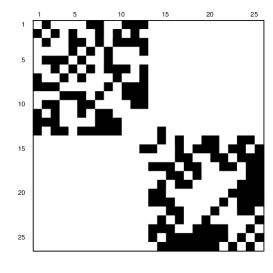
(a) $p_{\text{inter}}=0.01$, $sparse$=25.4%.

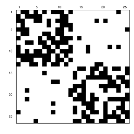
(b) $p_{\text{inter}}=0.05$, $sparse$=30%.

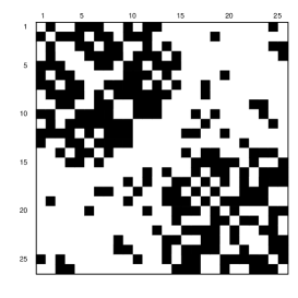
(c) $p_{\text{inter}}=0.15$, $sparse$=37%.

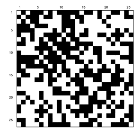
(d) $p_{\text{inter}}=0.4$, $sparse$=47.6%.

We simulate $Y_{1},\dots Y_{n}$ realizations of a Gaussian random variable $\mathcal{N}(0,\mathbf{M})$, for various values of sample size $n$. Edges are estimated applying correlation tests (P-2). 325 tests are needed in this framework. The four statistics described above as the four methods are applied, that is, Methods 1–3 and Method 4’. The level for the FWER control is fixed to $\alpha=5\%$. The non parametric bootstrap and the parametric bootstrap requires to fix the number of samples used in the estimation of quantiles. For non parametric bootstrap, the number of samples is denoted as BootRWand equal to 100. For parametric bootstrap, denoted MaxT, the number of samples is fixed to 1000. Resulting computational cost is high but less samples leads to an unsatisfying quality.

Our simulation procedure depends on the three main parameters: $\rho$, $p_{inter}$, and $n$. $\rho$ corresponds to the value of entries in the correlation matrices. This is related to the signal to noise ratio for the identification of edges in the graph. Indeed, when $\rho$ is low, it is harder to detect the correct edges. In the sequel, the simulations are displayed for two values of $\rho$: 0.1 and 0.2. Recall that because of the constraint on our model, it is not possible to choose larger values of $\rho$. $p_{inter}$ is defined as the number of edges between the two components of the stochastic block model. This is controlling the sparsity of the graph and equivalently the number of null hypotheses. When $p_{inter}$ increases, the number of null hypotheses decreases. For the Bonferroni procedure, this has a direct impact on the FWER. Finally, $n$ is the number of independent realizations available to estimate the correlations. $n$ and $\rho$ are linked by our main assumption on the convergence of the estimator (1). In the two following parts, results of simulations applied on all four methods and using different parameters in the model are given for both FWER and power.

3.2 Results on FWER control

The difference between $\rho=0.2$ and $\rho=0.1$ is illustrated on Figure 2 and Figure 4. It is clear that when $\rho=0.1$, all the proposed approaches provide empirical FWER much lower than the theoretical value fixed at 0.05 for any sample sizes and any sparsity.

The influence of the sample size $n$ relative to the use of a specific statistics is displayed on Figure 2 for $(T^{(1)}_{ij})_{1\leq i<j\leq p}$, Figure 4 for $(T^{(2)}_{ij})_{1\leq i<j\leq p}$, Figure 6 for $(T^{(3)}_{ij})_{1\leq i<j\leq p}$ and Figure 6 for $(T^{(4)}_{ij})_{1\leq i<j\leq p}$. Depending on the chosen statistics, for small sample sizes the FWER may not be controlled: this is due to the initial test procedure rather than the multiple correction. Indeed, tests (P-1) are based on the normality of the statistics $(T^{(k)}_{ij})_{1\leq i<j\leq p}$, $k=1,\dots,4$. As the Gaussian distribution is only satisfied asymptotically, the FWER control is valid only for sufficiently large values of $n$. The convergence of the Gaussian statistics $(T^{(4)}_{ij})_{1\leq i<j\leq p}$ is the slowest, and there is no control of FWER for $n\leq 200$. However, for the Student statistics $(T^{(2)}_{ij})_{1\leq i<j\leq p}$ the control of FWER is valid for $n\geq 200$. With the Fisher statistics $(T^{(2)}_{ij})_{1\leq i<j\leq p}$ only the case $n=50$ is not controlled, while the empirical statistics $(T^{(1)}_{ij})_{1\leq i<j\leq p}$ behaves well even for small sample sizes.

The advantage of using BootRW procedure lies in the fact that it does require a Gaussian distribution. As the quantile is evaluated on bootstrap resamples of the statistics, it corresponds to the effective distribution and not to the theoretical one. As a consequence, the FWER is controlled for all tests statistics, whatever the sample size but this comes with an increase of the computation time.

The comparison of step-down procedure with single step is also illustrated on the Figures 4 to 6. In particular, Figures 4, 6 and 6 show that the control for step-down MaxT is not always obtained. This results from numerical instability of the quantile estimation. Indeed, as discussed in Section 3.1, the number of bootstrap samples is critical. The numerical approximation is more critical for step-down procedures. It is shown in particular for sparse models and large sample sizes.

The empirical FWER slightly increases with the sparsity of the matrix. This is due to the link between the sparsity and the number of null hypotheses $m_{0}(P)$. The FWER level of multiple testing procedures usually increases with $m_{0}(P)$. For example, for Bonferroni procedure, the FWER is in fact controlled at level $\alpha\frac{m_{0}(P)}{m}$.

Figure 2: Empirical FWER on 10000 simulations, with respect to the sample size $n$, for empirical statistics, $T^{(1)}$. The four sparsity frameworks are considered. $\rho=0.2$.

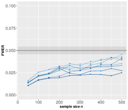
(a) Bonferroni

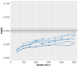
(b) Šidák

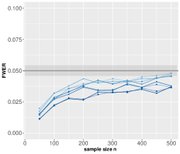
(c) BootRW

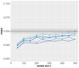
(d) MaxT

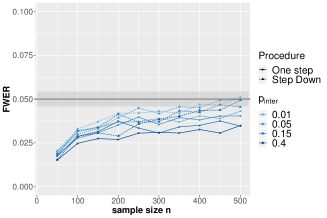
(e) Oracle MaxT

Figure 3: Empirical FWER on 10000 simulations, with respect to the sample size $n$, for empirical statistics, $T^{(1)}$. The four sparsity frameworks are considered. $\rho=0.1$.

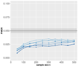
(a) Bonferroni

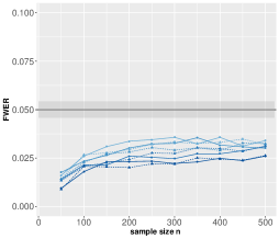
(b) Šidák

(c) BootRW

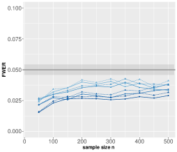
(d) MaxT

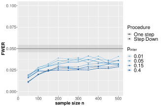
(e) Oracle MaxT

Figure 4: Empirical FWER on 10000 simulations, with respect to the sample size $n$, for Student statistics, $T^{(2)}$. The four sparsity frameworks are considered. $\rho=0.2$.

(a) Bonferroni

(b) Šidák

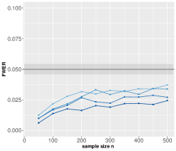
(c) BootRW

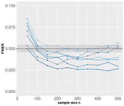
(d) MaxT

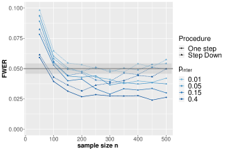
(e) Oracle MaxT

Figure 5: Empirical FWER on 10000 simulations, with respect to the sample size $n$, for Fisher statistics, $T^{(3)}$. The four sparsity frameworks are considered. $\rho=0.2$.

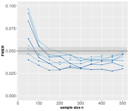
(a) Bonferroni

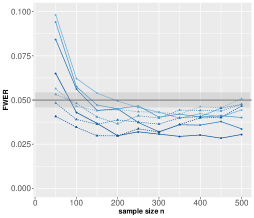
(b) Šidák

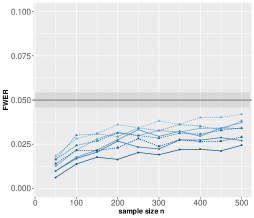
(c) BootRW

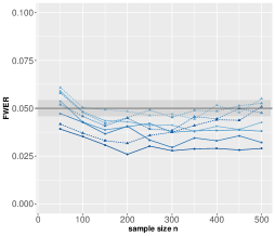
(d) MaxT

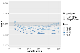
(e) Oracle MaxT

Figure 6: Empirical FWER on 10000 simulations, with respect to the sample size $n$, for Gaussian statistics, $T^{(4)}$. The four sparsity frameworks are considered. $\rho=0.2$.

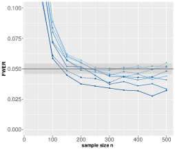
(a) Bonferroni

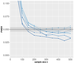
(b) Šidák

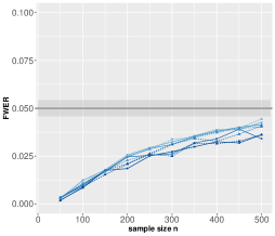
(c) BootRW

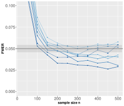
(d) MaxT

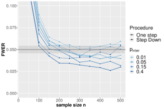
(e) Oracle MaxT

3.3 Results on power

This Section provides a detailed evaluation of the power of the multiple testing procedures on simulations. The quality is computed by the proportion of significant correlations detected, also called True Discovery Proportion, defined as

$$\frac{\lvert\mathcal{R}\cap\{\mathcal{H}\setminus\mathcal{H}_{0}\}\rvert}{\lvert\mathcal{H}\setminus\mathcal{H}_{0}\rvert},$$

where for every sets $A$ and $B$, $A\setminus B=\{x\in A:x\notin B\}$.

First, a crucial point in many edges detection procedures is the graph sparsity (for instance Bickel and Levina, 2008a , Ledoit et al., (2012), Ravikumar et al., (2011), Fan et al., (2016)). The sparsity is controlled here by the parameter $p_{inter}$: recall that the lower $p_{inter}$ is, the sparser the graph is. Figure 8 illustrates that with a multiple testing approach, the sparsity does not influence the power of the procedure, since the proportion of edges rightly detected is nearly constant with respect to the sparsity.

Of course clearly, Figure 8 shows that the power increases with the sample size $n$. Indeed, with small $n$, the procedures are not able to detect significant correlations because the statistical tests cannot discriminate the null and the alternative hypothesis. When the sample size is small, the variance of the empirical correlations on which the test statistics are based is high, see Figure 10.

Similarly, Figure 8 illustrates the failure of the procedures to detect significant correlations when the value of $\rho$ is small, here $\rho=0.1$. Again, this comes from the power of statistical tests rather than the multiple correction. Similar discussion can be found in Hero and Rajaratnam, (2011) (see e.g. Figure 2). Figures 10 and 10 give an insight of maximal power reachable in our setting, respectively with $\rho=0.2$ and $\rho=0.1$. It also illustrates that indeed the sparsity does not influence the support of the empirical correlations distributions, which explains the stability of the power with respect to sparsity.

Comparison between the power of the procedure with respect to the test statistics is displayed in Table 1. Only the case $\rho=0.2$, $p_{inter}=0.4$ and three values of sample size $n$ are considered for the sake of simplicity. Similar results are obtained in other settings. For all procedures except BootRW, the Student statistics $T^{(3)}$ is the most powerful statistic. Concerning BootRW, the empirical test statistics $T^{(1)}$ give the best results. Second-order statistic $T^{(4)}$ shows the lowest power for all multiple corrections.

Romano and Wolf, (2005)’s non parametric bootstrap BootRW has the advantage of controlling FWER independently on the statistic and the sample size. However it is less powerful than other step-down procedures. Results for step-down MaxT are high but this procedure may not control the FWER. The power of single-step parametric bootstrap BootRW is lower than Bonferroni and Šidák step-down procedures.

We observe that the empirical test statistics $T^{(1)}$ always control the FWER. Thus this choice seems particularly adequate. In addition, the most powerful multiple correction is step-down Šidák. If the sample size $n$ is sufficiently large so that the FWER control is acquired ($n\geq 200$ for the sparse model, see Figure 4), step-down Šidák correction with Student statistics based tests gives the highest power. An advantage of using Bonferroni and Šidák procedures lies in the fact that the computational time is very small.

Figure 7: Empirical power on 10000 simulations, with respect to the sample size $n$, for empirical statistics, $T^{(1)}$. The four sparsity frameworks are considered. $\rho=0.2$.

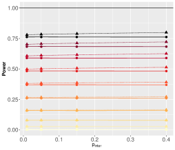
(a) Bonferroni

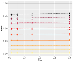
(b) Šidák

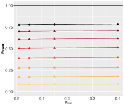
(c) BootRW

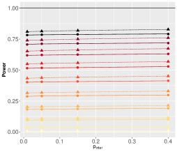
(d) MaxT

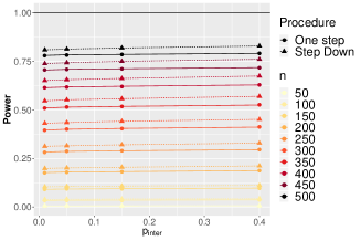
(e) Oracle MaxT

Figure 8: Empirical power on 10000 simulations, with respect to the sample size $n$, for empirical statistics, $T^{(1)}$. The four sparsity frameworks are considered. $\rho=0.1$.

(a) Bonferroni

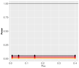
(b) Šidák

(c) BootRW

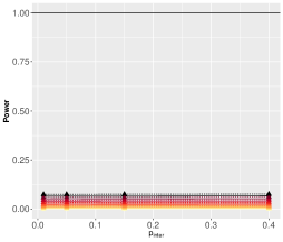
(d) MaxT

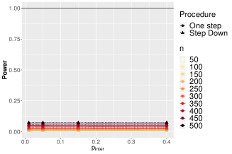
(e) Oracle MaxT

Table 1: Empirical power on 10000 simulations, with respect to the multiple testing correction for sample size $n$ equal to 100, 300, 500. The adjacency matrix is given by $p_{inter}=0.4$, i.e. with the lowest sparsity. $\rho=0.2$. The left hand side value is the empirical power obtained with single-step methods and the right hand side value is obtained with step-down method.

$n=100$
	Bonferroni	Šidák	BootRW	MaxT	oracle MaxT
Empirical $T^{(1)}$	0.028 $|$ 0.028	0.028 $|$ 0.028	0.032 $|$ 0.032	0.036 $|$ 0.038	0.034 $|$ 0.036
Student   $T^{(2)}$	0.047 $|$ 0.047	0.047 $|$ 0.047	0.024 $|$ 0.024	0.042 $|$ 0.045	0.044 $|$ 0.047
Fisher     $T^{(3)}$	0.047 $|$ 0.040	0.047 $|$ 0.040	0.024 $|$ 0.029	0.040 $|$ 0.043	0.040 $|$ 0.042
Gaussian  $T^{(4)}$	0.026 $|$ 0.026	0.026 $|$ 0.026	0.006 $|$ 0.006	0.023 $|$ 0.025	0.024 $|$ 0.026
$n=300$
	Bonferroni	Šidák	BootRW	MaxT	oracle MaxT
Empirical $T^{(1)}$	0.370 $|$ 0.392	0.373 $|$ 0.394	0.400 $|$ 0.399	0.405 $|$ 0.422	0.401 $|$ 0.423
Student   $T^{(2)}$	0.400 $|$ 0.400	0.403 $|$ 0.403	0.357 $|$ 0.357	0.387 $|$ 0.424	0.389 $|$ 0.421
Fisher     $T^{(3)}$	0.400 $|$ 0.412	0.403 $|$ 0.414	0.357 $|$ 0.378	0.394 $|$ 0.422	0.393 $|$ 0.422
Gaussian  $T^{(4)}$	0.339 $|$ 0.359	0.342 $|$ 0.362	0.311 $|$ 0.311	0.328 $|$ 0.360	0.330 $|$ 0.358
$n=500$
	Bonferroni	Šidák	BootRW	MaxT	oracle MaxT
Empirical $T^{(1)}$	0.762 $|$ 0.800	0.764 $|$ 0.802	0.786 $|$ 0.786	0.787 $|$ 0.813	0.786 $|$ 0.814
Student   $T^{(2)}$	0.776 $|$ 0.776	0.778 $|$ 0.778	0.752 $|$ 0.752	0.766 $|$ 0.818	0.767 $|$ 0.816
Fisher     $T^{(3)}$	0.776 $|$ 0.807	0.778 $|$ 0.809	0.752 $|$ 0.767	0.775 $|$ 0.816	0.774 $|$ 0.816
Gaussian  $T^{(4)}$	0.746 $|$ 0.787	0.748 $|$ 0.789	0.751 $|$ 0.751	0.737 $|$ 0.793	0.738 $|$ 0.792

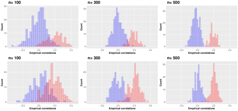
Figure 9: Histograms of the empirical correlations. Blue histograms correspond to true null hypothesis and red histograms correspond to observations under the alternative hypothesis $\rho=0.2$. On the first row the sparsity parameter satisfies $p_{inter}=0.01$ and on the second row $p_{inter}=0.4$.

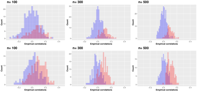
Figure 10: Histograms of the empirical correlations. Blue histograms correspond to true null hypothesis and red histograms correspond to observations under the alternative hypothesis $\rho=0.1$. On the first row the sparsity parameter satisfies $p_{inter}=0.01$ and on the second row $p_{inter}=0.4$.

4 Real data

We apply our methods on real data sets from neuroscience. We use functional Magnetic Resonance images (fMRI) of both dead and alive rats. The datasets are freely available 10.5281/zenodo.2452871 (Becq et al., 2020a, , Becq et al., 2020b, ). The aim is to estimate the brain connectivity, that is the significant correlations between brain regions where fMRI signals are recorded. For this data set, we know that for dead rats we are under the full null hypothesis. Thus the estimated graphs should be empty. We also expect non-empty graphs for alive rats.

4.1 Description of the dataset

Functional Magnetic Resonance Images (fMRI) were acquired for both dead and alive rats in Pawela et al., (2008). Rats $1$ to $4$ were scanned dead and rats $5$ to $11$ were scanned alive under anesthetic. The duration of the scanning is 30 minutes with a time repetition of 0.5 second so that $3600$ time points are available at the end of experience. After preprocessing as explained in Pawela et al., (2008), $51$ time series for each rat were extracted. Each time series capture the functioning of a given region of the rat brain based on an anatomical atlas.

The time series resulting from fMRI experiments are nonstationary with long memory properties, which is not convenient from a mathematical point of view. To avoid such properties, the correlation coefficients are estimated in the wavelet transform domain and then the statistical tests are based on wavelet correlation coefficients, as described in Achard and Gannaz, (2016), Moulines et al., (2007).

First we are decomposing each time series using a wavelet basis and then for each wavelet scale we are studying all the possible pairs of correlations.

Let $(\phi(\cdot),\psi(\cdot))$ be respectively a father and a mother wavelets. At a given resolution $j\geq 0$, for $k\in\mathbb{Z}$, we define the dilated and translated functions $\phi_{j,k}(\cdot)=2^{-j/2}\phi(2^{-j}\cdot-k)$ and $\psi_{j,k}(\cdot)=2^{-j/2}\psi(2^{-j}\cdot-k)$. Let $\tilde{\mathbf{X}}(t)=\sum_{k\in\mathbb{Z}}\mathbf{X}(k)\phi(t-k)$. The wavelet coefficients of the process $\mathbf{X}$ are defined by

$$\mathbf{W}_{j,k}=\int_{\mathbb{R}}\tilde{\mathbf{X}}(t)\psi_{j,k}(t)dt\quad j\geq 0,\;k\in\mathbb{Z}.$$

For given $j\geq 0$ and $k\in\mathbb{Z}$, $\mathbf{W}_{j,k}$ is a $p$-dimensional vector

$$\mathbf{W}_{jk}=\begin{pmatrix}W_{j,k}(1)&W_{j,k}(2)&\dots&W_{j,k}(p)\end{pmatrix},$$

where $W_{j,k}(\ell)=\int_{\mathbb{R}}\tilde{X_{\ell}}(t)\psi_{j,k}(t)dt$.

Let $z$ be the Fisher transform, for all $x$, $-1\leq x\leq 1$,

$$z(x):=\frac{1}{2}\log\frac{1+x}{1-x}=\tanh^{-1}(x).$$

We fix a scale $j$ and the tests are based on the correlation of wavelets coefficients at scale $j$. Define

$${\rho_{\ell m}}(j) =\frac{\gamma_{\ell m}(j)}{(\gamma_{\ell\ell}(j)\gamma_{mm}(j))^{1/2}},\quad\text{\leavevmode\nobreak\ with\leavevmode\nobreak\ }\gamma_{\ell m}(j):=\int\mathcal{H}_{j}(\lambda)\,f_{\ell m}(\lambda)\,d\,\lambda$$

$$\widehat{\rho_{\ell m}}(j) =\frac{\sum_{k=0}^{n_{j}}(W_{j,k}(\ell)W_{j,k}(m))}{(\sum_{k=0}^{n_{j}}W^{2}_{j,k}(\ell)\sum_{k=0}^{n_{j}}W^{2}_{j,k}(m))^{1/2}},$$

where $\mathcal{H}_{j}$ denotes the squared gain filter of wavelet transform at scale $j$. Note that quantities $\rho_{\ell m}(j)$ depends on the memory properties of the time series, as described among others in Achard and Gannaz, (2019).

The convergence of wavelet correlations with Fisher transform is given by the following property.

Proposition 4.1 (Achard et al., (2019)).

Under the regularity hypotheses on the wavelet transform, the estimator of empirical correlation verifies

$$\sqrt{(n_{j}-3)}(z(\widehat{\rho_{\ell m}}(j))-z(\rho_{\ell m}(j)))\mathop{\longrightarrow}^{\mathcal{L}}\mathcal{N}(0,1)\,;$$ (15)

A discussion on the choice of the relevant scale for analysis can be found in Achard et al., (2019). From there and the literature in neuroscience, it is convenient and adequate to focus on low frequencies where the best signal-to-noise ratio is obtained. Here we will focus on wavelet scale 4 corresponding to the frequency interval [0.06 ; 0.12] Hz. The number of available wavelet coefficients is then $n=122$.

For a given rat $k\in\{1,\dots,11\}$, let $\mathbf{W}^{(k)}_{\ell}$ be the vector of wavelet coefficients at scale 4 for the time series of the $\ell$-th cerebral region, $\ell=1,\dots,51$ and $k=1,\dots,11$. The vector $\mathbf{W}^{(k)}_{\ell}$ has length 122. We introduce $(z(\widehat{\rho}_{\ell m}^{(k)}))_{\ell,m=1,\dots,p}$ the matrix of Fisher statistics evaluated on the wavelet coefficients processes $\mathbf{W}^{(k)}_{\ell}$ and $\mathbf{W}^{(k)}_{m}$. With previous notations, for a given rat $k$, for all $(\ell,m)$, $z(\widehat{\rho}_{\ell m}^{(k)})$ corresponds to the Fisher statistics $T^{(3)}_{\ell m}$ evaluated with $Y^{(\ell)}=\mathbf{W}^{(k)}_{\ell}$.

The aim is then to test if there are connections between each pairs of cerebral region at a given scale $j\geq 0$. The following tests should thus be applied, for each rat $k$, at the scale $j=4$ in this study:

$$H_{0,\ell m}(j):\rho_{\ell m}(j)=0\text{\leavevmode\nobreak\ against \leavevmode\nobreak\ }H_{1,\ell m}(j):\rho_{\ell m}(j)\neq 0,$$ (P-3)

all $1\leq\ell<m\leq p$. for Since the whole brain of rats are aggregated into $p=51$ cerebral regions, we have to deal with $m=1275$ tests for each of the 11 rats.

4.2 Numerical results

As explained above, we consider tests (P-3) for each rat, on wavelet coefficients at scale 4. A rejection of hypothesis $(H_{0,\ell m})$ means a significant correlation between the activities of cerebral regions $\ell$ and $m$.

Examples of correlation matrices obtained are given in Figure 11. Even if dead rats correlation matrices are much closer to identity matrices than correlation matrices on alive rats, some non zero values are observed and a test of significance is needed.

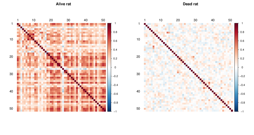
Figure 11: Examples of two correlation matrices between wavelet coefficients obtained at scale 4 for an alive rat (left) and a dead rat (right).

Boxplots of empirical correlations are displayed in Figure 12. They state a clear difference between dead and alive rats correlation distributions. An important remark is also that in real application the alternative non zero value is not constant and can be much higher than the value taken in our simulation (which was at the maximum equal to 0.2). Indeed for each alive rat, we observe instances of empirical correlation higher than $0.8$. We thus expect a signal-to-noise ratio higher in the application than in our simulation, and therefore good power performances of multiple testing.

Figure 12: Boxplots of empirical correlations between wavelet coefficients obtained at scale 4 (i.e., the frequency interval [0.06 ; 0.12] Hz) on fMRI recordings of rats. The first four rats are dead while rats 5 to 11 are alive.

Since we consider Fisher statistics $T^{(3)}$, with sample size $n=122$, the simulation study displays that the FWER is controlled for all procedures (see Figure 6). Next the most powerful approach is step-down MaxT parametric bootstrap in general, but for small samples Šidák procedure is competitive. Moreover the numerical instability on the quantile estimation for MaxT as well as the computation time give preference to step-down Šidák multiple correction (see Table 1).

We thus define the rejection set of (P-3) applying step-down Šidák’s multiple testing procedure on Fisher statistics. As we have to deal with $1275$ tests for each rat, a multiple testing procedure is necessary. Without a multiple testing correction on $p$-values, the inferred graph is highly biased, as illustrated by the clearly non-empty graph for a dead rat displayed in Figure 13. A similar result was obtained on the detection of an activation on fMRI recordings for a dead salmon in Bennett et al., (2011).

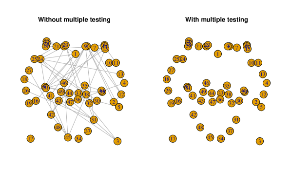
Figure 13: Illustration of the necessity to make multiple correction for a given dead rat: Left: estimate of the connectivity graph between brain regions without correction for multiple testing, using the raw values of the empirical correlations; Right: estimation of the same graph using multiple testing on correlations (Step-down Šidák procedure with Fisher statistics) ; $\alpha=5\%$.

It is not possible in general to evaluate the accuracy of procedures on real dataset because of the lack of ground truth. However, since there is actually no cerebral activity in a brain of a dead rat, all null hypotheses to be tested are true nulls and the number of rejected hypotheses must be equal to zero in this case. Indeed, we obtain that the number of significant correlations is zero or near to zero for dead rats (see Table 2). We can still observe a few remaining connections in the graphs from very close brain regions. This is due to the fact that the fMRI scanner is introducing spurious correlations between neighboring parts of the brain. Some examples of estimated graphs for dead rats and alive rats are displayed in Figure 14. Edges for dead rats are not visible because they are between nodes at very short distance.

Dead rat	1	2	3	4
$|E|$	4	1	0	2

Alive rat	5	6	7	8	9	10	11
$|E|$	444	236	201	595	385	410	318

Table 2: Number of rejected null hypotheses $|E|$ (that is also the number of estimate edges) obtained by step-down Šidák procedure on Fisher statistics, evaluated at scale 4 with a threshold $\alpha=5\%$.

Note that there is a high variability of the results with respect to rats. The highest number of detections is obtained for the rats $5$ and $8$ with more than 33% of edges. For the others, the number of detections is between $15\%$ and $33\%$.

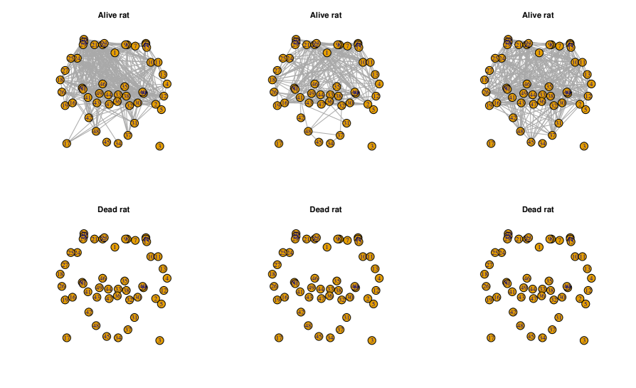
Figure 14: Examples of graphs obtained at scale 4 for some alive rats (first row) and some dead rats (second row). Step-down Šidák correction was used with Fisher statistics.

5 Asymptotic control of the FDR for correlation tests

Another usual criterion for multiple testing is False Discovery Rate (FDR). Denoting $\mathcal{Q}$ the proportion of false discoveries, for all $P\in\mathcal{P}$, we define the FDR as

$$\text{ FDR}(\mathcal{R},P)=\mathbb{E}[\mathcal{Q}],\text{ where }\mathcal{Q}=\frac{|\mathcal{R}\cap\mathcal{H}_{0}(P)|}{|\mathcal{R}|\vee 1}.$$ (16)

“$|\mathcal{R}|\vee 1$” is the maximum between $|\mathcal{R}|$ and 1 when no hypothesis is rejected ($|\mathcal{R}|=0$).

A well-known procedure for controlling FDR is Benjamini-Hochberg’s (BH), Benjamini and Hochberg, (1995). Denoting $(p_{(i)})_{1\leq i\leq m}$ the family of the ordered $p$-values, we can write the index set of rejected null hypotheses by the BH procedure as

$$\mathcal{R}_{BH}=\Big{\{}i\in\{1,\ldots,m\}:p_{i}\leq\alpha\widehat{k}/m\Big{\}},$$ (17)

where $\widehat{k}=\max\{k\in\{0,\ldots,m\}:p_{(k)}\leq\alpha k/m\}$ with the convention $p_{(0)}=0$.

We can prove that the limit of the FDR of the BH procedure is equal to the FDR of the limiting experience.

Theorem 5.1.

Suppose

$$\forall P\in\mathcal{P},\,\sqrt{n}\left(\>\widehat{\theta}_{n,\cdot}-\theta(P)\right)\overset{d}{\longrightarrow}P_{\infty}.$$ (18)

Then for all $P\in\mathcal{P}$,

$$\underset{n\to+\infty}{\lim}\text{ }\rm{FDR}(\textit{P})=\text{ }\rm{FDR}(\textit{P}_{\infty}).$$

In particular, if $P_{\infty}$ is Positive Regression Dependent on each one from a Subset (PRDS) on $\{1\leq i\leq m:c_{i}=0\}$, then Benjamini and Hochberg, (1995) states that the asymptotic control of FDR by BH procedure is acquired. In the one-sided Gaussian testing framework, the PRDS assumption is satisfied whenever $\Sigma_{ij}\geq 0$, for all $(i,j)$, see Benjamini and Yekutieli, (2001). However, this result is not helpful for testing correlations in two-sided Gaussian setting. For instance, Yekutieli, (2008) gives some examples of non-PRDS two-sided Gaussian tests. We refer to Roux, (2018), Chapter 4, for an overview of results of the BH procedure in two-sided Gaussian setting.

Resulting from a simulation study, we can state that indeed the matrix $\Omega(\Gamma)$ of Proposition 2.1 does not provide a positive structure dependence in general. There is no clear property to test if $p$-values are PRDS. We decided to examine a stronger but more easily verifiable assumption, that is, Multivariate Total Positivity of order 2 (MTP₂), see Karlin and Rinott, (1980). The evaluation of the proportion of MTP₂ distributions is based on Theorem $3.1$ and Theorem $3.1^{\prime}$ of Karlin and Rinott, (1981), which give necessary and sufficient condition on the matrix $\Gamma$ (resp. $\Omega(\Gamma)$) for $|X|$ (resp. $(|\rho_{h}|)_{h\in\mathcal{H}}$) having an MTP₂ distribution. We generate $100,000$ covariance $d$-matrices $\Gamma$ using the R-package ClusterGeneration of Joe, (2006), and we evaluate the occurrence of MTP₂ distributions on these $100,000$ matrices. Results are displayed in Table 3. The proportion of the vector of the absolute value of correlation coefficients of $X$, that is, $(|\rho_{h}|)_{h\in\mathcal{H}}$, having an MTP₂ distribution is evaluated in two different cases: when $|X|$ does not have an MTP₂ distribution (third column of Table 3) and when $|X|$ has an MTP₂ distribution (fourth column of Table 3).

Distribution of:	$|X|$	$(|\rho_{h}|)_{h\in\mathcal{H}}$
		without MTP2 constraint on $|X|$	with MTP2 constraint on $|X|$
$d=3$	5100	10223	0
$d=4$	82	38	0
$d=5$	0	0	$\cdot$

Table 3: Occurrence of MTP₂ distributions on 100,000 simulations. The dot means that the quantity is not computable.

As shown in Table 3, the MTP₂ constraint seems to be a very restrictive constraint (see the second column of Table 3). Moreover, even if the absolute value of the observed vector $X$ has an MTP2₂ distribution, the transformation $\Omega$ does not preserve the positive dependence structure (see the last column of Table 3) for the correlation coefficients.

In Romano et al., (2008), the authors proposed both subsampling and bootstrap procedures that control the false discovery rate (FDR) under dependence, especially for the two-sided testing problem (P-1). Unfortunately, their methods require that all the $p$-values under the alternative are equal to zero. Finally, Cai and Liu, (2016) developed a truncated bootstrap alternative to BH for correlation tests. The idea is to estimate the threshold index $\widehat{k}$ in (16) by bootstrap evaluations of the FDR. They add a truncation based on the asymptotic Gaussian property of tests statistics. Theoretical control is obtained, under sparsity assumptions.

Conclusion

This work was motivated by a real data application in neuroscience. Our aim is to identify the connectivity graphs of brain areas by testing if the correlation between recordings of pairs of brain regions is significant. Our statistical modeling includes asymptotically Gaussian statistics and multiple corrections because many simultaneous tests are applied (here, 1275 in the application). Hence in this work we have studied multiple testing when statistics are asymptotically Gaussian, and possibly correlated. Four multiple testing procedures are presented: Bonferroni, Šidák, Romano-Wolf non parametric bootstrap (BootRW) and a parametric bootstrap (MaxT). For each of these methods, we verify that the FWER is asymptotically controlled. Besides, special attention is given to the case of correlation testing. A simulation study then highlights problems that may be encountered in applications. First for many statistics, a sufficient sample size is necessary to ensure the control of FWER. Next the parametric bootstrap suffers from numerical instability. Interestingly, the sparsity of the false hypothesis does not influence the quality of the procedures. Finally, we apply a multiple testing correction on a real dataset, inferring the connectivity graphs of small animals from resting state fMRI recordings. The recordings for dead animals enable us to verify that the obtained results are coherent by finding a nearly empty graph. In contrast alive animals connectivity graphs are not empty. This confirms the utility of our approach for real data applications.

Appendix A Proofs

A.1 Proof of Proposition 1.1

For all $P\in\mathcal{P}$,

$$\textrm{FWER}\Big{(}\mathcal{R}^{bonf}_{\alpha},P\Big{)}=\mathbb{P}\left(\bigcup_{i\in\mathcal{H}_{0}(P)}\{p_{n,i}\leq\alpha/m\}\right).$$

Thus,

$$\underset{n\to+\infty}{\lim}\textrm{FWER}\Big{(}\mathcal{R}^{bonf}_{\alpha},P\Big{)}\leq\displaystyle{\sum_{i\in\mathcal{H}_{0}(P)}}\frac{\alpha}{m}\leq\frac{\alpha m_{0}(P)}{m}\leq\alpha.$$

A.1.1 Proof of Proposition 1.2

In order to prove Proposition 1.2, we first need the following result.

Proposition A.1.

For all $x>0$, for all $P\in\mathcal{P}$,

$$\underset{n\to+\infty}{\lim}\left\{\mathbb{P}\left(\sqrt{n}\,\left|\>\widehat{\theta}_{n,i}\left(\mathbb{X}^{(n)}\right)-\theta_{i}(P)\right|\,\leq\,x,\text{ for all }i\in\mathcal{H}_{0}(P)\right)\right\}\geq(2\Phi(x)-1)^{m_{0}(P)}.$$ (19)

Proof.

Let $Z_{i}=\lim_{n\to+\infty}\sqrt{n}\,\left|\>\widehat{\theta}_{n,i}\left(\mathbb{X}^{(n)}\right)-\theta_{i}(P)\right|$. Then $Z=(Z_{i})_{1\leq i\leq m_{0}(P)}$ is $m_{0}(P)$-dimensional random vector with a multivariate Gaussian distribution $\mathcal{N}_{m_{0}(P)}\Big{(}0,(\Sigma)_{i,i^{\prime}\in\mathcal{H}_{0}(P)}\Big{)}$. Let $B=\Big{\{}z\in\mathbb{R}^{m_{0}(P)}:\|z\|_{\infty}\leq x\Big{\}}$. Let $\partial B$ denote the frontier of the set $B$. For all $x>0$,

$$\mathbb{P}(Z\in\partial B) =\mathbb{P}(||Z||_{\infty}=x)$$

$$=\mathbb{P}\bigg{(}\sup_{1\leq j\leq m_{0}(P)}|Z_{j}|=x\bigg{)}$$

$$\leq\mathbb{P}\Big{(}\exists j\in\{1,\ldots,m_{0}(P)\}:|Z_{j}|=x\Big{)}$$

$$\leq\sum_{j=1}^{m_{0}(P)}\mathbb{P}(|Z_{j}|=x)$$

$$\leq 0,$$

By Portmanteau’s lemma (Billingsley,, 2013), it follows that for all $P\in\mathcal{P}$,

$$\underset{n\to+\infty}{\lim}\mathbb{P}\left(\sup_{i\in\mathcal{H}_{0}(P)}\sqrt{n}\lvert\widehat{\theta}_{n,\cdot}-\theta(P)\rvert\leq x\right)=\mathbb{P}(\|Z\|_{\infty}\leq x),$$

Applying (6), for all $P\in\mathcal{P}$,

$$\underset{n\to+\infty}{\lim}\mathbb{P}\left(\sup_{i\in\mathcal{H}_{0}(P)}\sqrt{n}\lvert\widehat{\theta}_{n,\cdot}-\theta(P)\rvert\leq x\right)\geq\Big{[}\mathbb{P}(|Z_{1}|\leq x)\Big{]}^{m_{0}(P)},$$

which concludes the proof. ∎

We now are in position to prove Proposition 1.2.

For all invertible $\Sigma$, for all $P\in\mathcal{P}$,

$$\mathrm{FWER}(\mathcal{R}^{s}_{\alpha},P) =\mathbb{P}\Big{(}\exists\>i\in\mathcal{H}_{0}(P):|T_{n,i}|>c_{\alpha}^{s}\Big{)}$$

$$=1-\mathbb{P}\Big{(}\forall\>i\in\mathcal{H}_{0}(P),|T_{n,i}|\leq c_{\alpha}^{s}\Big{)}$$

$$=1-\mathbb{P}\Big{(}\lVert(T_{n,i})_{i\in\mathcal{H}_{0}(P)}\rVert_{\infty}\leq c_{\alpha}^{s}\Big{)}$$

Using Proposition A.1,

$$\underset{n\to+\infty}{\lim}\mathrm{FWER}(\mathcal{R}^{s}_{\alpha},P)\leq 1-(2\Phi(c_{\alpha}^{s})-1)^{m_{0}(P)}\leq\alpha.$$

A.2 Proof of Proposition 1.3

Under $P$, the matrix $\Sigma$ is assumed to be invertible. Therefore $\left(T_{n,i}\left(\mathbb{X}^{(n)}\right)\right)_{i\in\mathcal{H}_{0}(P)}$ has a non-degenerate asymptotic distribution. The result then follows from Theorem 7 of Romano and Wolf, (2005).

A.2.1 Proof of Proposition 1.4

Let $P\in\mathcal{P}$. Denote by $\left.\mathcal{N}_{m}(0,\Sigma)\right\lvert_{\mathcal{H}_{0}(P)}$ the restriction of the Gaussian distribution $\mathcal{N}_{m}(0,\Sigma)$ on $\mathcal{H}_{0}(P)$, namely $\mathcal{N}_{m_{0}(P)}\Big{(}0,(\Sigma)_{i,i^{\prime}\in\mathcal{H}_{0}(P)}\Big{)}$.

First, since the functions $(T_{n,i})_{i\in\mathcal{H}_{0}(P)}\xrightarrow[n\to+\infty]{\quad d\quad}\left.\mathcal{N}_{m}(0,\Sigma)\right\lvert_{\mathcal{H}_{0}(P)}$ and $x\mapsto\|x\|_{\infty}$ for $x\in\mathbb{R}^{|\mathcal{H}_{0}(P)|}$ are continuous, then by the continuous mapping theorem, we have that

$$\|(T_{n,i})_{i\in\mathcal{H}_{0}(P)})\|_{\infty}\xrightarrow[n\to+\infty]{\quad d\quad}\|\left.\mathcal{N}_{m}(0,\Sigma)\right\lvert_{\mathcal{H}_{0}(P)}\|_{\infty}.$$ (20)

Second, let us establish that

$$t_{n,\alpha}(\widehat{\Sigma}_{n})\overset{\mathbb{P}}{\longrightarrow}t_{\alpha}(\Sigma).$$ (21)

Let $x\in\mathbb{R}$. For all $n\in\mathbb{N}$, we introduce the cumulative distribution functions $\varphi_{x}(\widehat{\Sigma}_{n})$ and $\varphi_{x}(\Sigma)$, defined by

$$\varphi_{x}(\widehat{\Sigma}_{n}) =\mathbb{P}(\|\widehat{\Sigma}_{n}^{1/2}\xi\|_{\infty}\leq x\mid\widehat{\Sigma}_{n}),$$

$$\varphi_{x}(\Sigma) =\mathbb{P}(\|\Sigma^{1/2}\xi\|_{\infty}\leq x),$$

where $\xi\sim\mathcal{N}_{m}(0,I_{m})$.

The Cramér-Wold device (Gut, (2012), Theorem 10.5) involves $\widehat{\Sigma}_{n}^{1/2}\xi\xrightarrow[n\to+\infty]{d}\Sigma^{1/2}\xi$ and thus, by the continuous mapping theorem, $\|\widehat{\Sigma}_{n}^{1/2}\xi\|_{\infty}\xrightarrow[n\to+\infty]{d}\|\Sigma^{1/2}\xi\|_{\infty}$. In addition, applying Portmanteau’s lemma, we obtain that $\varphi_{x}(\widehat{\Sigma}_{n})$ converges in probability to $\varphi_{x}(\Sigma)$ when $n$ goes to infinity. Therefore, for all $\epsilon>0$,

$$\varphi_{t_{\alpha}(\Sigma)-\epsilon}(\widehat{\Sigma}_{n})\overset{\mathbb{P}}{\longrightarrow}\varphi_{t_{\alpha}(\Sigma)-\epsilon}(\Sigma).$$ (22)

Let $\epsilon>0$. One has

$$\mathbb{P}\Big{(}t_{n,\alpha}(\widehat{\Sigma}_{n})\leq t_{\alpha}(\Sigma)-\epsilon\Big{)}$$

$$=\mathbb{P}\Big{(}\varphi_{t_{\alpha}(\Sigma)-\epsilon}(\widehat{\Sigma}_{n})\geq 1-\alpha\Big{)}$$

$$=\mathbb{P}\Big{(}\varphi_{t_{\alpha}(\Sigma)-\epsilon}(\widehat{\Sigma}_{n})-\varphi_{t_{\alpha}(\Sigma)-\epsilon}(\Sigma)\geq 1-\alpha-\varphi_{t_{\alpha}(\Sigma)-\epsilon}(\Sigma)\Big{)}.$$

Write $\varphi_{t_{\alpha}(\Sigma)-\epsilon}(\Sigma)=1-\alpha-\beta$, with $\beta>0$. The right-hand side is bounded by

$$\mathbb{P}\Big{(}\varphi_{t_{n,\alpha}(\Sigma)-\epsilon}(\widehat{\Sigma}_{n})-\varphi_{t_{n,\alpha}(\Sigma)-\epsilon}(\Sigma)\geq\beta\Big{)} \leq\mathbb{P}\Big{(}\big{|}\varphi_{t_{n,\alpha}(\Sigma)-\epsilon}(\widehat{\Sigma}_{n})-\varphi_{t_{n,\alpha}(\Sigma)-\epsilon}(\Sigma)\big{|}\geq\beta\Big{)}.$$

Then, convergence (21) follows from (22).

We now finally establish the asymptotic FWER control for the procedure $\mathcal{R}^{MaxT}$. By definition,

$$\text{FWER}(\mathcal{R}^{MaxT}_{\alpha},P)=\mathbb{P}\Big{(}\|(T_{n,i})_{i\in\mathcal{H}_{0}(P)}\|_{\infty}\geq t_{n,\alpha}(\widehat{\Sigma}_{n})\Big{)}.$$

For all $\delta>0$, this quantity is bounded by

$$\mathbb{P}\Big{(}\|(T_{n,i})_{i\in\mathcal{H}_{0}(P)}\|_{\infty}>t_{\alpha}(\Sigma)-\delta\Big{)}+\mathbb{P}\Big{(}t_{\alpha}(\widehat{\Sigma}_{n})\leq t_{n,\alpha}(\Sigma)-\delta\Big{)}.$$

Then, using (20) and (21), we have

$$\underset{n\to+\infty}{\limsup}\text{ FWER}(\mathcal{R}^{MaxT}_{\alpha},P)\leq\mathbb{P}\Big{(}\|\left.\mathcal{N}_{m}(0,\Sigma)\right\lvert_{\mathcal{H}_{0}(P)}\|_{\infty}>t_{\alpha}(\Sigma)-\delta\Big{)}.$$

Letting $\delta$ tend to 0 we obtain the asymptotic control.

A.3 Proof of Proposition 1.5

Let $P\in\mathcal{P}$. By (12), there exists an event $\mathcal{E}$, such that $\mathcal{E}\cap\mathcal{H}_{0}(P)\subseteq\mathcal{E}\setminus{\mathcal{R}_{\mathcal{H}_{0}(P)}}$ and

$$\mathbb{P}(\mathcal{E})\xrightarrow[n\to+\infty]{}1-\alpha.$$ (23)

For all $j\geq 0$, $\mathcal{H}_{0}(P)\subseteq\mathcal{C}_{j}$ implies that $\mathcal{R}_{\mathcal{H}_{0}(P)}\supseteq\mathcal{R}_{\mathcal{C}_{j}}$ by (13). Thus we have $\mathcal{E}\setminus\mathcal{R}_{\mathcal{H}_{0}(P)}\subseteq\mathcal{E}\setminus\mathcal{R}_{\mathcal{C}_{j}}$. Consequently, $\mathcal{E}\cap{\mathcal{H}_{0}(P)}\subseteq\mathcal{C}_{j+1}$. Since $\mathcal{H}_{0}(P)\subseteq\mathcal{C}_{0}=\{1,\ldots,m\}$, a recurrence gives $\mathcal{E}\cap\mathcal{H}_{0}(P)\subseteq\mathcal{E}\cap\mathcal{C}_{j}$ for all $j\geq 0$. It results that $\mathcal{E}\cap\mathcal{H}_{0}(P)\subseteq\mathcal{E}\setminus\mathcal{R}_{{\mathcal{C}}_{\infty}}$. Finally, using convergence (23),

$$\mathbb{P}(\mathcal{H}_{0}(P)\subseteq\{1,\dots,m\}\setminus\mathcal{R}_{{\mathcal{C}}_{\infty}})\xrightarrow[n\to+\infty]{}1-\alpha.$$

Since the left-hand side is equal to $1-\text{FWER}\Big{(}R_{{\mathcal{C}}_{\infty}},P\Big{)}$, Proposition 1.5 is proved.

A.4 Proof of Theorem 5.1

Let $f:\mathbb{R}\rightarrow[0,1],x\mapsto 1-\Phi(x+c)$ and $Y^{(n)}=\sqrt{n}\Big{(}\widehat{\theta}_{n,\cdot}-\theta(P)\Big{)}$. For all $k\in\{1,\ldots,m\}$, for all $i\in\mathcal{H}_{0}(P)$, define the set $\mathcal{B}_{k,i}$ as

$$\mathcal{B}_{k,i}=\Big{\{}y\in\mathbb{R}^{m}:\widehat{k}\leq k-1\,\mathrm{and}\,f(y_{i})\leq\alpha(k-1)/m\Big{\}}$$

For all $y\in\mathbb{R}^{m}$, we can sort the m-dimensional vector $(f(y_{1}),f(y_{2}),\dots,f(y_{m}))$ as $f(y)_{(1)}\leq f(y)_{(2\leq\dots\leq f(y)_{(m)})}$. The set $\mathcal{B}_{k,i}$ can be rewritten as

$$\mathcal{B}_{k,i}=\Big{\{}y\in\mathbb{R}^{m}:f(y)_{(j)}>\alpha j/m\text{ for }j=k,\ldots,m,\,\mathrm{and}\,f(y_{i})\leq\alpha(k-1)/m\Big{\}}.$$

Denote $\eta$ the Lebesgue’s measure and $\partial\mathcal{B}_{k,i}$ the frontier of the set $\mathcal{B}_{k,i}$. We want to prove that for all $k\in\{1,\ldots,m\}$, for all $i\in\mathcal{H}_{0}(P)$, $\eta(\partial\mathcal{B}_{k,i})=0$. For all $k\in\{1,\ldots,m\}$, for all $i\in\mathcal{H}_{0}(P)$, we have

$$\eta(\partial\mathcal{B}_{k,i}) =\eta\bigg{(}\partial\bigg{[}\bigg{(}\bigcap_{j=k}^{m}\Big{\{}y:f(y)_{(j)}>\alpha j/m\Big{\}}\bigg{)}\bigcap\Big{\{}y:f(y_{i})\leq\alpha(k-1)/m\Big{\}}\bigg{]}\bigg{)}$$

$$\leq\eta\bigg{(}\bigg{(}\bigcup_{j=k}^{m}\partial\Big{\{}y:f(y)_{(j)}>\alpha j/m\Big{\}}\bigg{)}\bigcup\partial\Big{\{}y:f(y_{i})\leq\alpha(k-1)/m\Big{\}}\bigg{)}$$

$$\leq\sum_{j=k}^{m}\eta\big{(}\{y:f(y)_{(j)}=\alpha j/m\}\big{)}+\eta\big{(}\{y:f(y_{i})=\alpha(k-1)/m\}\big{)}$$

$$\leq\sum_{l=1}^{m}\sum_{j=k}^{m}\eta\big{(}\{y:f(y_{l})=\alpha j/m\}\big{)}+\eta\big{(}\{y:f(y_{i})=\alpha(k-1)/m\}\big{)}.$$

Since the right-hand side is null, equality $\eta(\partial\mathcal{B}_{k,i})=0$ holds. Consequently for all $k\in\{1,\ldots,m\}$, for all $i\in\mathcal{H}_{0}(P)$, $\mathbb{P}(Y\in\partial\mathcal{B}_{k,i})=0$. Using Portmanteau’s lemma, it follows that

$$\underset{n\to+\infty}{\lim}\mathbb{P}\Big{(}Y^{(n)}\in\mathcal{B}_{k,i}\Big{)}=\mathbb{P}(Y\in\mathcal{B}_{k,i}).$$

If $\mathcal{B}_{k,i}^{\prime}=\Big{\{}y\in\mathbb{R}^{m}:\widehat{k}\leq k-1\,\mathrm{and}\,f(y_{i})\leq\alpha k/m\Big{\}}$, with a similar reasoning we can prove that

$$\underset{n\to+\infty}{\lim}\mathbb{P}\Big{(}Y^{(n)}\in\mathcal{B}_{k,i}^{\prime}\Big{)}=\mathbb{P}(Y\in\mathcal{B}_{k,i}^{\prime}).$$

Therefore, we obtain

$$\text{ FDR}(P)$$

$$=\sum_{i\in\mathcal{H}_{0}(P)}\sum_{k=1}^{m}\frac{1}{k}\Bigg{[}\mathbb{P}\bigg{(}\widehat{k}\leq k,f\Big{(}Y^{(n)}_{i}\Big{)}\leq\alpha k/m\bigg{)}-\mathbb{P}\bigg{(}\widehat{k}\leq k-1,f\Big{(}Y^{(n)}_{i}\Big{)}\leq\alpha k/m\bigg{)}\Bigg{]}$$

$$=\sum_{i\in\mathcal{H}_{0}(P)}\sum_{k=1}^{m}\frac{1}{k}\Bigg{[}\mathbb{P}\Big{(}Y^{(n)}\in\mathcal{B}_{k+1,i}\Big{)}-\mathbb{P}\Big{(}Y^{(n)}\in\mathcal{B}_{k,i}^{\prime}\Big{)}\Bigg{]}.$$

Taking the limit in the previous expression leads to

$$\underset{n\to+\infty}{\lim}\text{ FDR}(P) =\sum_{i\in\mathcal{H}_{0}(P)}\sum_{k=1}^{m}\frac{1}{k}\Bigg{[}\mathbb{P}\Big{(}Y\in\mathcal{B}_{k+1,i}\Big{)}-\mathbb{P}\Big{(}Y\in\mathcal{B}_{k,i}^{\prime}\Big{)}\Bigg{]}$$

$$=\text{FDR}(P_{\infty}).$$

References

• Achard etΒ al., (2019) Achard, S., Borgnat, P., Gannaz, I., and Roux, M. (2019). Wavelet-based graph inference using multiple testing. In Ville, D. V.Β D., Papadakis, M., and Lu, Y.Β M., editors, Wavelets and Sparsity XVIII, volume 11138, pages 322 – 336. International Society for Optics and Photonics, SPIE.
• Achard and Gannaz, (2016) Achard, S. and Gannaz, I. (2016). Multivariate wavelet whittle estimation in long-range dependence. Journal of Time Series Analysis, 37(4):476–512. arXiv preprint arXiv:1412.0391.
• Achard and Gannaz, (2019) Achard, S. and Gannaz, I. (2019). Wavelet-based multivariate Whittle estimation, comparison with Fourier: multiwave. Journal of Statistical Software, 69(6):1–31.
• Achard etΒ al., (2006) Achard, S., Salvador, R., Whitcher, B., Suckling, J., and Bullmore, E. (2006). A resilient, low-frequency, small-world human brain functional network with highly connected association cortical hubs. The Journal of Neuroscience, 26(1):63–72. 00831.
• Aitkin, (1969) Aitkin, M.Β A. (1969). Some tests for correlation matrices. Biometrika, pages 443–446.
• Anderson, (2003) Anderson, T. (2003). An Introduction to Multivariate Statistical Analysis. John Wiley & Sons, third edition edition.
• Banerjee etΒ al., (2006) Banerjee, O., Ghaoui, L.Β E., d’Aspremont, A., and Natsoulis, G. (2006). Convex optimization techniques for fitting sparse Gaussian graphical models. In Proceedings of the 23rd international conference on Machine learning, pages 89–96. ACM.
• (8) Becq, G. G. J.-P.Β C., Barbier, E., and Achard, S. (2020a). Brain networks of rats under anesthesia using resting-state fmri: comparison with dead rats, random noise and generative models of networks. Journal of Neural Engineering.
• (9) Becq, G. J.-P., Habet, T., Collomb, N., Faucher, M., Delon-Martin, C., Coizet, V., Achard, S., and Barbier, E.Β L. (2020b). Functional connectivity is preserved but reorganized across several anesthetic regimes. NeuroImage, 219:116945.
• Benjamini and Hochberg, (1995) Benjamini, Y. and Hochberg, Y. (1995). Controlling the false discovery rate: a practical and powerful approach to multiple testing. Journal of the Royal Statistical Society. Series B (Methodological), pages 289–300.
• Benjamini and Yekutieli, (2001) Benjamini, Y. and Yekutieli, D. (2001). The control of the false discovery rate in multiple testing under dependency. Annals of statistics, pages 1165–1188.
• Bennett etΒ al., (2011) Bennett, C.Β M., Baird, A.Β A., Miller, M.Β B., and Wolford, G.Β L. (2011). Neural correlates of interspecies perspective taking in the post-mortem atlantic salmon: an argument for proper multiple comparisons correction. Journal of Serendipitous and Unexpected Results, 1:1–5.
• (13) Bickel, P.Β J. and Levina, E. (2008a). Covariance regularization by thresholding. The Annals of Statistics, 36(6):2577–2604.
• (14) Bickel, P.Β J. and Levina, E. (2008b). Regularized estimation of large covariance matrices. The Annals of Statistics, pages 199–227.
• Billingsley, (2013) Billingsley, P. (2013). Convergence of probability measures. John Wiley & Sons.
• Bland and Altman, (1995) Bland, J.Β M. and Altman, D.Β G. (1995). Multiple significance tests: the bonferroni method. Bmj, 310(6973):170.
• Bonferroni, (1935) Bonferroni, C.Β E. (1935). Il calcolo delle assicurazioni su gruppi di teste. Tipografia del Senato.
• Cai etΒ al., (2011) Cai, T., Liu, W., and Luo, X. (2011). A constrained $\ell$-1 minimization approach to sparse precision matrix estimation. Journal of the American Statistical Association, 106(494):594–607.
• Cai and Liu, (2016) Cai, T.Β T. and Liu, W. (2016). Large-scale multiple testing of correlations. Journal of the American Statistical Association, 111(513):229–240.
• Csardi and Nepusz, (2006) Csardi, G. and Nepusz, T. (2006). The igraph software package for complex network research. InterJournal, Complex Systems:1695.
• Cvetkovic etΒ al., (2004) Cvetkovic, D., CvetkoviΔ‡, D.Β M., Rowlinson, P., Simic, S., and SimiΔ‡, S. (2004). Spectral generalizations of line graphs: On graphs with least eigenvalue-2, volume 314. Cambridge University Press.
• Drton and Perlman, (2004) Drton, M. and Perlman, M.Β D. (2004). Model selection for Gaussian concentration graphs. Biometrika, 91(3):591–602.
• Drton and Perlman, (2007) Drton, M. and Perlman, M.Β D. (2007). Multiple testing and error control in Gaussian graphical model selection. Statistical Science, pages 430–449.
• Dudoit etΒ al., (2003) Dudoit, S., Shaffer, J.Β P., Boldrick, J.Β C., etΒ al. (2003). Multiple hypothesis testing in microarray experiments. Statistical Science, 18(1):71–103.
• Dudoit and Van DerΒ Laan, (2007) Dudoit, S. and Van DerΒ Laan, M.Β J. (2007). Multiple testing procedures with applications to genomics. Springer Science & Business Media.
• Fan etΒ al., (2016) Fan, J., Liao, Y., and Liu, H. (2016). An overview of the estimation of large covariance and precision matrices. The Econometrics Journal, 19(1):C1–C32.
• Finner and Gontscharuk, (2009) Finner, H. and Gontscharuk, V. (2009). Controlling the familywise error rate with plug-in estimator for the proportion of true null hypotheses. Journal of the Royal Statistical Society: Series B (Statistical Methodology), 71(5):1031–1048.
• Friedman etΒ al., (2008) Friedman, J., Hastie, T., and Tibshirani, R. (2008). Sparse inverse covariance estimation with the graphical lasso. Biostatistics, 9(3):432–441.
• Gannaz, (2019) Gannaz, I. (2019). TestCor: FWER and FDR Controlling Procedures for Multiple Correlation Tests. R package version 0.0.2.0.
• Genz and Bretz, (2009) Genz, A. and Bretz, F. (2009). Computation of Multivariate Normal and t Probabilities. Lecture Notes in Statistics. Springer-Verlag, Heidelberg.
• Goeman and Solari, (2010) Goeman, J.Β J. and Solari, A. (2010). The sequential rejection principle of familywise error control. The Annals of Statistics, pages 3782–3810.
• Guillot and Rajaratnam, (2012) Guillot, D. and Rajaratnam, B. (2012). Retaining positive definiteness in thresholded matrices. Linear Algebra and its Applications, 436(11):4143–4160.
• Gut, (2012) Gut, A. (2012). Probability: a graduate course, volumeΒ 75. Springer Science & Business Media.
• Hero and Rajaratnam, (2011) Hero, A. and Rajaratnam, B. (2011). Large-scale correlation screening. Journal of the American Statistical Association, 106(496):1540–1552.
• Holm, (1979) Holm, S. (1979). A simple sequentially rejective multiple test procedure. Scandinavian journal of statistics, pages 65–70.
• Joe, (2006) Joe, H. (2006). Generating random correlation matrices based on partial correlations. Journal of Multivariate Analysis, 97(10):2177–2189.
• Johnstone, (2001) Johnstone, I.Β M. (2001). On the distribution of the largest eigenvalue in principal components analysis. Annals of statistics, pages 295–327.
• Karlin and Rinott, (1980) Karlin, S. and Rinott, Y. (1980). Classes of orderings of measures and related correlation inequalities. I. Multivariate totally positive distributions. Journal of Multivariate Analysis, 10(4):467–498.
• Karlin and Rinott, (1981) Karlin, S. and Rinott, Y. (1981). Total positivity properties of absolute value multinormal variables with applications to confidence interval estimates and related probabilistic inequalities. The Annals of Statistics, pages 1035–1049.
• Kolaczyk, (2009) Kolaczyk, E.Β D. (2009). Statistical analysis of network data. Springer.
• KrΓ€mer etΒ al., (2009) KrΓ€mer, N., SchΓ€fer, J., and Boulesteix, A.-L. (2009). Regularized estimation of large-scale gene association networks using graphical gaussian models. BMC bioinformatics, 10(1):384.
• Ledoit etΒ al., (2012) Ledoit, O., Wolf, M., etΒ al. (2012). Nonlinear shrinkage estimation of large-dimensional covariance matrices. The Annals of Statistics, 40(2):1024–1060.
• Markov etΒ al., (2013) Markov, N.Β T., Ercsey-Ravasz, M., VanΒ Essen, D.Β C., Knoblauch, K., Toroczkai, Z., and Kennedy, H. (2013). Cortical high-density counterstream architectures. Science, 342(6158):1238406.
• Meinshausen and BΓΌhlmann, (2006) Meinshausen, N. and BΓΌhlmann, P. (2006). High-dimensional graphs and variable selection with the Lasso. Annals of Statistics, 34(3):1436–1462.
• Moulines etΒ al., (2007) Moulines, E., Roueff, F., and Taqqu, M. (2007). On the spectral density of the wavelet coefficients of long memory time series with application to the log-regression estimation of the memory parameter. Journal of Time Series Analysis, 28:155–187.
• Nadarajah and Kotz, (2008) Nadarajah, S. and Kotz, S. (2008). Exact distribution of the max/min of two gaussian random variables. IEEE Transactions on very large scale integration (VLSI) systems, 16(2):210–212.
• Newman, (2010) Newman, M. E.Β J. (2010). Networks An Introduction. Oxford university press.
• Pawela etΒ al., (2008) Pawela, C.Β P., Biswal, B.Β B., Cho, Y.Β R., Kao, D.Β S., Li, R., Jones, S.Β R., Schulte, M.Β L., Matloub, H.Β S., Hudetz, A.Β G., and Hyde, J.Β S. (2008). Resting-state functional connectivity of the rat brain. Magnetic Resonance in Medicine, 59(5):1021–1029.
• Ravikumar etΒ al., (2011) Ravikumar, P., Wainwright, M.Β J., Raskutti, G., Yu, B., etΒ al. (2011). High-dimensional covariance estimation by minimizing $\ell_{1}$-penalized log-determinant divergence. Electronic Journal of Statistics, 5:935–980.
• Rohe etΒ al., (2011) Rohe, K., Chatterjee, S., Yu, B., etΒ al. (2011). Spectral clustering and the high-dimensional stochastic blockmodel. The Annals of Statistics, 39(4):1878–1915.
• Romano etΒ al., (2008) Romano, J.Β P., Shaikh, A.Β M., and Wolf, M. (2008). Control of the false discovery rate under dependence using the bootstrap and subsampling. Test, 17(3):417.
• Romano and Wolf, (2005) Romano, J.Β P. and Wolf, M. (2005). Exact and approximate stepdown methods for multiple hypothesis testing. Journal of the American Statistical Association, 100(469):94–108.
• Rothman etΒ al., (2008) Rothman, A.Β J., Bickel, P.Β J., Levina, E., Zhu, J., etΒ al. (2008). Sparse permutation invariant covariance estimation. Electronic Journal of Statistics, 2:494–515.
• Roux, (2018) Roux, M. (2018). Graph inference by multiple testing with application to Neuroimaging. Ph.d, UniversitΓ© Grenoble Alpes, France.
• SchΓ€fer and Strimmer, (2005) SchΓ€fer, J. and Strimmer, K. (2005). An empirical bayes approach to inferring large-scale gene association networks. Bioinformatics, 21(6):754–764.
• Ε idΓ‘k, (1967) Ε idΓ‘k, Z. (1967). Rectangular confidence regions for the means of multivariate normal distributions. Journal of the American Statistical Association, 62(318):626–633.
• Steiger and Hakstian, (1982) Steiger, J.Β H. and Hakstian, A.Β R. (1982). The asymptotic distribution of elements of a correlation matrix: Theory and application. British Journal of Mathematical and Statistical Psychology.
• Wasserman, (2013) Wasserman, L. (2013). All of statistics: a concise course in statistical inference. Springer Science & Business Media.
• Westfall and Young, (1993) Westfall, P.Β H. and Young, S.Β S. (1993). Resampling-based multiple testing: Examples and methods for p-value adjustment, volume 279. John Wiley & Sons.
• Wu and Pourahmadi, (2009) Wu, W.Β B. and Pourahmadi, M. (2009). Banding sample autocovariance matrices of stationary processes. Statistica Sinica, pages 1755–1768.
• Yekutieli, (2008) Yekutieli, D. (2008). False discovery rate control for non-positively regression dependent test statistics. Journal of Statistical Planning and Inference, 138(2):405–415.