Second Order Accurate Hierarchical Approximate Factorization of Sparse SPD Matrices

Abstract

We describe a second-order accurate approach to sparsifying the off-diagonal blocks in the hierarchical approximate factorizations of sparse symmetric positive definite matrices. The norm of the error made by the new approach depends quadratically, not linearly, on the error in the low-rank approximation of the given block. The analysis of the resulting two-level preconditioner shows that the preconditioner is second-order accurate as well. We incorporate the new approach into the recent Sparsified Nested Dissection algorithm [SIAM J. Matrix Anal. Appl., 41 (2020), pp. 715-746], and test it on a wide range of problems. The new approach halves the number of Conjugate Gradient iterations needed for convergence, with almost the same factorization complexity, improving the total runtimes of the algorithm. Our approach can be incorporated into other rank-structured methods for solving sparse linear systems.

65F08, 65F05, 65F50, 15A23, 15A12

1 Introduction

Hierarchical approximate factorizations are a recent group of approaches to solving sparse linear systems

$$\begin{matrix}Ax=b,&A\in\mathbb{R}^{n\times n},&b\in\mathbb{R}^{n}\end{matrix}$$

such as those arising from discretized partial differential equations (PDEs). These methods (also called the fast hierarchical solvers) include, among others, Hierarchical Interpolative Factorization [18, 9], LoRaSp [26, 40], or Sparsified Nested Dissection [4]. Significant focus in their development has been on the symmetric positive definite (SPD) case (also [29, 7, 23, 6]) on which we concentrate in this paper.

Fast hierarchical solvers repeatedly sparsify selected off-diagonal blocks while performing the block Gaussian elimination of $A$. Without such sparsifications, Gaussian elimination is not practical for large-scale problems. To recall why, assume $A$ is a sparse SPD matrix of the form

$$A=\begin{pmatrix}A_{11}&A_{12}\\ A_{12}^{\top}&A_{22}\end{pmatrix}$$

Let $A_{11}=L_{1}L_{1}^{\top}$ be the Cholesky decomposition. Eliminating the variables corresponding to $A_{11}$ leads to

$$A=\begin{pmatrix}L_{1}&\\ A_{12}^{\top}L_{1}^{-\top}&I\end{pmatrix}\begin{pmatrix}I&\\ &A_{22}-A_{12}^{\top}A_{11}^{-1}A_{12}\end{pmatrix}\begin{pmatrix}L_{1}^{\top}&L_{1}^{-1}A_{12}\\ &I\end{pmatrix}$$

where the Schur complement $S=A_{22}-A_{12}^{\top}A_{11}^{-1}A_{12}$ in general contains new fill-in entries and loses the original sparsity of $A_{22}$. If we keep eliminating variables naively, the amount of fill-in will eventually make further computations too expensive, with $\mathcal{O}(n^{3})$ complexity of factorizing the matrix. The amount of fill-in can be minimized using an ordering of variables, e.g., based on the nested dissection algorithm [11, 24]. Under mild assumptions, nested dissection can reduce the complexity down to $\mathcal{O}(n^{3/2}),$ or $\mathcal{O}(n^{2}),$ on problems corresponding to, respectively, 2D, and 3D grids. However, such complexity is still only practical for relatively small problems.

On the other hand, the fill-in arising from elimination typically has the low-rank property. Namely, certain off-diagonal blocks in the Schur complement have quickly decaying singular values, and can be sparsified. To illustrate the sparsification of a single block $S_{12}$ in the Schur complement $S$, we first scale the leading block

$$S=\begin{pmatrix}S_{11}&S_{12}\\ S_{12}^{\top}&S_{22}\end{pmatrix}=\begin{pmatrix}Z_{1}&\\ &I\end{pmatrix}\begin{pmatrix}I&\widehat{S}_{12}\\ \widehat{S}_{12}^{\top}&S_{22}\end{pmatrix}\begin{pmatrix}Z_{1}^{\top}&\\ &I\end{pmatrix}=ZS^{\prime}Z^{\top}$$

where $S_{11}=Z_{1}Z_{1}^{\top}$ is the Cholesky decomposition, and $\widehat{S}_{12}=Z_{1}^{-1}S_{12}$. Sparsification then involves computing a rank-revealing decomposition of $\widehat{S}_{12}$, to obtain an orthogonal matrix $Q=\begin{pmatrix}Q_{1}&Q_{2}\end{pmatrix}$ such that $\|Q_{1}^{T}\widehat{S}_{12}\|=E$ where $\|E\|$ is small. In other words, $Q_{2}$ approximates the range of $\widehat{S}_{12}$. Then

(1) $$S^{\prime}= \begin{pmatrix}I&\widehat{S}_{12}\\ \widehat{S}_{12}^{\top}&S_{22}\end{pmatrix}=\begin{pmatrix}Q_{1}&Q_{2}\\ &&I\end{pmatrix}\begin{pmatrix}I&&E\\ &I&Q_{2}^{\top}\widehat{S}_{12}\\ E^{\top}&\widehat{S}_{12}^{\top}Q_{2}&S_{22}\end{pmatrix}\begin{pmatrix}Q_{1}^{\top}&\\ Q_{2}^{\top}&\\ &I\end{pmatrix}$$

(2) $$\approx \begin{pmatrix}Q&\\ &I\end{pmatrix}\underbrace{\begin{pmatrix}I&&\\ &I&Q_{2}^{\top}\widehat{S}_{12}\\ \ &\widehat{S}_{12}^{\top}Q_{2}&S_{22}\end{pmatrix}}_{\begin{matrix}S^{\prime\prime}\end{matrix}}\begin{pmatrix}Q^{\top}&\\ &I\end{pmatrix}=S^{\prime}+\mathcal{O}(\|E\|)$$

The $E$ and $E^{\top}$ terms are dropped, and $S^{\prime\prime}$ is sparser than $S$. The approaches based on such sparsification scheme include, among others, [18, 29, 9, 4, 7, 23, 40, 6]. These algorithms approximately factorize matrices arising from discretized PDEs, typically in $\mathcal{O}(n)$ or $\mathcal{O}(n\log{n})$ operations, repeatedly sparsifying the matrix during the factorization. The result is an approximation $A\approx LL^{\top}$ where $L$ is a product of block-triangular and block-diagonal matrices, so that $L^{-1}L^{-\top}\approx A^{-1}$ can be efficiently applied, typically in $\mathcal{O}(n)$ operations. This operator is then used as a preconditioner in a Krylov subspace method, such as Conjugate Gradient [17] or GMRES [27]

In this paper, we describe a sparsification approach which makes an $\mathcal{O}(\|E\|^{2})$ error in approximating $S^{\prime}$, while restoring the same amount of sparsity. The general idea is to only drop the $E^{\top}E$ term when eliminating the leading variables in Eq. 1:

(3) $$S^{\prime}= \begin{pmatrix}I&\widehat{S}_{12}\\ \widehat{S}_{12}^{\top}&S_{22}\end{pmatrix}=\begin{pmatrix}Q&\\ E^{\top}&I\end{pmatrix}\begin{pmatrix}I&&\\ &I&Q_{2}^{\top}\widehat{S}_{12}\\ &\widehat{S}_{12}^{\top}Q_{2}&S_{22}-E^{\top}E\end{pmatrix}\begin{pmatrix}Q^{\top}&E\\ &I\end{pmatrix}$$

(4) $$\approx \begin{pmatrix}Q&\\ E^{\top}&I\end{pmatrix}\underbrace{\begin{pmatrix}I&&\\ &I&Q_{2}^{\top}\widehat{S}_{12}\\ \ &\widehat{S}_{12}^{\top}Q_{2}&S_{22}\end{pmatrix}}_{\begin{matrix}S^{\prime\prime}\end{matrix}}\begin{pmatrix}Q^{\top}&E\\ &I\end{pmatrix}=S^{\prime}+\mathcal{O}(\|E\|^{2})$$

The matrix $S^{\prime\prime}$ is the same as in Eq. 2. The operator $\widetilde{L}^{-\top}\widetilde{L}^{-1}\approx A^{-1}$ resulting from the approximation, is significantly more accurate than before, but only moderately more expensive to apply (each term $\begin{pmatrix}Q&\\ &I\end{pmatrix}$ going into the product $\widetilde{L}$ is replaced by $\begin{pmatrix}Q&\\ E^{\top}&I\end{pmatrix}$ which is sparse, well-conditioned, and whose inverse can be efficiently applied).

We incorporate the new sparsification approach into the recent Sparsified Nested Dissection algorithm (spaND) [4]. The algorithm uses the approximation Eq. 2, which we replace by approximations based on Eq. 3. While we focus on the SPD case, in which spaND is guaranteed to complete and be stable without pivoting, the new sparsification approach is applicable also in the general case.

1.1 Context

Low-rank approximations of the off-diagonal or fill-in matrix blocks is a key ingredient of rank-structured hierarchical methods for solving linear systems that arise from boundary integral equations or discretized PDEs. These methods include accelerated direct methods based on $\mathcal{H}$-matrices [28], hierarchical semi-separable (HSS) matrices [5, 35, 36, 33], the hierarchical off-diagonal low-rank framework (HODLR) [2, 20], and others [13, 1]. At moderate accuracies, these methods can be used as general-purpose preconditioners [15, 16, 12]. In particular, [22, 37, 38] obtained efficient and robust preconditioners for SPD matrices based on approximation Eq. 2. A version for general matrices was described in [21]. Hierarchical approximate factorizations [18, 9, 23, 26, 29, 4] are recent approaches suitable for sparse systems. These methods do not require special data-sparse matrix formats that underlie some of the previous approaches. As mentioned above, they explicitly compute an approximate factorization of $A$ into a product of sparse block-triangular and block-diagonal matrices.

1.2 Contributions

The contributions of this paper are the following:

1. We describe the new approach resulting in a quadratic approximation error as in Eq. 3. We present two variants: a more accurate one (called the full second-order scheme) in which the error term is exactly squared compared to Eq. 2, and a sparser approach (called superfine second-order scheme) which also has a second-order accuracy.

2. We compute expressions for the condition number of the preconditioned systems for two-level preconditioners resulting from Eq. 2 (which we call the first-order scheme), and the new approach. (The two-level preconditioner is obtained by inverting exactly the matrix resulting from sparsifying a single block.) The condition number when using the full second-order scheme depends quadratically, while the condition number when using the first-order scheme depends linearly, on the same term, whose norm is smaller than one.

3. For the two-level preconditioners, we show that the theoretical bound on the relative error in the preconditioned Conjugate Gradient (PCG) when using the full second-order scheme is exactly squared, compared to the first-order scheme. This translates into halving the bound on the iteration count.

4. For right-hand sides that satisfy certain constraints, we also prove that, for the two-level preconditioners used with PCG, the residual at the $k$-th iteration when using the full second-order scheme is exactly the same as the residual at the $2k$-th iteration, when using the first-order scheme. As a result the convergence is two times faster at each step of PCG. While the constraints are not satisfied exactly in practice, we empirically observe similar behavior in our test cases (see below).

5. We incorporate the new approach into the Sparsified Nested Dissection algorithm (spaND) [4]. Our benchmarks demonstrate that the new methods involve a minor cost when computing the preconditioner.

6. We evaluate the action of the operators $I-MA$ resulting from applying the first- and second-order schemes in spaND (which returns the preconditioning operator $M$), on the eigenvectors of the constant-coefficient Laplace equation. We observe that the improvement in the accuracy on most of the spectrum is consistent with the two-level preconditioner analysis.

7. We perform a study of PCG counts and runtimes when using spaND, as a function of matrix size on high-contrast Laplacians, and run the algorithm on all large SPD matrices from the University of Florida sparse matrix (SuiteSparse) collection [8]. In all cases, the new approach improves the runtimes of spaND. In particular, consistently among all tested cases, the number of iterations of PCG needed for convergence is almost exactly halved, as predicted by the two-level preconditioner analysis.

8. We also observe that, for a given test case and accuracy parameter, the plot of the 2-norm of the residual in PCG as a function of iteration $k$ when using the full second-order scheme, is approximately the same as the one obtained by plotting for $k$ the $2k$-th residual when using the first-order scheme. This is consistent with the theoretical result mentioned in Item 4.

The paper is organized as follows. Our main theoretical results (Items 1, 2, 3, and 4 above) are in Section 2. The description of the spaND algorithm (Item 5) is in Section 3. The experimental results (Items 6, 7, and 8) are in Section 4, followed by conclusions in Section 5.

2 First- and second-order approximation schemes using the low-rank property

We now describe the approximation scheme Eq. 2 and the new approaches resulting in Eq. 3.

2.1 First-order scheme

Consider a sparse SPD matrix of the form

(5) $$A=\begin{pmatrix}I&A_{12}&\\ A_{21}&A_{22}&A_{23}\\ &A_{32}&A_{33}\end{pmatrix}$$

with a low-rank off-diagonal structure. That is, assume that $A_{12}=A_{21}^{\top}$ has quickly decaying singular values. One can exploit this fact to approximately eliminate a number of variables from the system without introducing any fill-in. To this end, one computes an orthogonal rank-revealing decomposition of $A_{12}$ (e.g., the rank-revealing QR or SVD), to obtain a square orthogonal matrix $Q=\begin{pmatrix}Q_{f}&Q_{c}\end{pmatrix}$ such that $Q_{c}$ is a matrix approximating the range of $A_{12}$. In other words, $\|E\|=\mathcal{O}(\varepsilon)$, where $E=Q_{f}^{\top}A_{12}$, but $Q_{f}$ should have as many columns as possible. The first-order scheme is defined by the following approximation, used in [4, 37, 38, 29, 6]

(6) $$A= \begin{pmatrix}Q_{f}&Q_{c}&\\ &&I&\\ &&&I\end{pmatrix}\begin{pmatrix}I&&E&\\ &I&Q_{c}^{\top}A_{12}&\\ E^{\top}&A_{21}Q_{c}&A_{22}&A_{23}\\ &&A_{32}&A_{33}\\ \end{pmatrix}\begin{pmatrix}Q_{f}^{\top}&&\\ Q_{c}^{\top}&&\\ &I&\\ &&I\end{pmatrix}$$

(7) $$\approx \begin{pmatrix}Q_{f}&Q_{c}&\\ &&I&\\ &&&I\end{pmatrix}\begin{pmatrix}I&&\\ &I&Q_{c}^{\top}A_{12}\\ &A_{21}Q_{c}&A_{22}&A_{23}\\ &&A_{32}&A_{33}\\ \end{pmatrix}\begin{pmatrix}Q_{f}^{\top}&&\\ Q_{c}^{\top}&&\\ &I&\\ &&I\end{pmatrix}$$

A number of leading variables (corresponding to $Q_{f}$) no longer interact with other variables, and are therefore decoupled. These variables are called the fine variables and are denoted by $f$ (the variables corresponding to $Q_{c}$ are called the coarse variables, denoted by $c$). The error in approximating $A$ is given by

(8) $$\mathcal{E}_{1}=\begin{pmatrix}Q&&\\ &I&\\ &&I\end{pmatrix}\begin{pmatrix}&&E&\\ &&&\\ E^{\top}&&&\\ &&&\end{pmatrix}\begin{pmatrix}Q^{\top}&&\\ &I&\\ &&I\end{pmatrix}=\mathcal{O}(\|E\|)=\mathcal{O}(\varepsilon)$$

We note that instead of orthogonal transformations, triangular matrices can also be used (see for example the Hierarchical Interpolative Factorization [18, 9, 23] or Recursive Skeletonization Factorization [25]).

2.2 Second-order scheme

The full second-order scheme is obtained by making an error in the Schur complement only, when eliminating the fine variables exactly:

(9) $$A= \begin{pmatrix}Q_{f}&Q_{c}&&\\ E^{\top}&&I&\\ &&&I\end{pmatrix}\begin{pmatrix}I&&&\\ &I&Q_{c}^{\top}A_{12}&\\ &A_{21}Q_{c}&A_{22}-E^{\top}E&A_{23}\\ &&A_{32}&A_{33}\end{pmatrix}\begin{pmatrix}Q_{f}^{\top}&E&\\ Q_{c}^{\top}&&\\ &I&\\ &&I\end{pmatrix}$$

(10) $$\approx \begin{pmatrix}Q_{f}&Q_{c}&&\\ \mathbf{E}^{\top}&&I&\\ &&&I\end{pmatrix}\begin{pmatrix}I&&&\\ &I&Q_{c}^{\top}A_{12}&\\ &A_{21}Q_{c}&A_{22}&A_{23}\\ &&A_{32}&A_{33}\end{pmatrix}\begin{pmatrix}Q_{f}^{\top}&\mathbf{E}&\\ Q_{c}^{\top}&&\\ &I&\\ &&I\end{pmatrix}$$

where we highlighted in bold the new terms appearing in the outer matrices (compared to Eq. 7). The error in approximating $A$ this time is

(11) $$\mathcal{E}_{2}= \begin{pmatrix}Q_{f}&Q_{c}&&\\ E^{\top}&&I&\\ &&&I\end{pmatrix}\begin{pmatrix}&&\\ &-E^{\top}E&\\ &&\end{pmatrix}\begin{pmatrix}Q_{f}^{\top}&E&\\ Q_{c}^{\top}&&\\ &I&\\ &&I\end{pmatrix}$$

(12) $$= \begin{pmatrix}&&\\ &-E^{\top}E&\\ &&\end{pmatrix}=\mathcal{O}(\|E\|^{2})=\mathcal{O}(\varepsilon^{2})$$

The middle matrix in Eq. 10 is the same as in Eq. 7. It is SPD, if $A$ is. In fact, its smallest eigenvalue is at least as large as the smallest eigenvalue of the middle matrix in Eq. 9, i.e., in the exact Cholesky factorization, because a symmetric negative semi-definite term $-E^{\top}E,$ is dropped. This is called the implicit Schur compensation, and makes the approximation stable [37, 4].

Notice also that because of the assumed sparsity of $A$, the outer matrices in Eq. 10 involve only a moderate number of additional nonzero entries as compared to the first-order scheme of Eq. 7. In a related problem, where $A$ is a dense rank-structured matrix, the full second-order scheme would in general result in a dense factorization (albeit efficiently obtained).

The assumption that the leading block in Eq. 5 is the identity matrix, i.e., $A_{11}=I$, is not limiting. If it is not the case, we scale the leading block

(13) $$A=\begin{pmatrix}Z_{1}&&\\ &I&\\ &&I\end{pmatrix}\begin{pmatrix}I&Z_{1}^{-1}A_{12}&\\ A_{21}Z_{1}^{-\top}&A_{22}&A_{23}\\ &A_{32}&A_{33}\end{pmatrix}\begin{pmatrix}Z_{1}^{\top}&&\\ &I&\\ &&I\end{pmatrix}$$

where $A_{11}=Z_{1}Z_{1}^{\top}$ is the (exact) Cholesky decomposition. In fact, such prescaling is an essential part of the algorithm, and improves its accuracy and robustness [6, 4, 9].

2.2.1 Superfine second-order scheme

We can further drop smallest entries of $E$ to obtain a second-order scheme in which the outer matrices are sparser. The matrix $Q=\begin{pmatrix}Q_{c}&Q_{f}\end{pmatrix}$, the set of coarse variables $c$, and the set of decoupled fine variables $f$, remain the same. However, we further split $Q_{f}=\begin{pmatrix}Q_{f_{1}}&Q_{f_{2}}\end{pmatrix}$ where $Q_{f_{1}}$ spans the space approximating the left singular vectors of $A_{12}$ whose corresponding singular values are sufficiently small to be immediately neglected (we therefore call $f_{1}$ the set of superfine variables). More precisely, we can choose $Q_{f_{1}}$ and $Q_{f_{2}}$ so that $\|E_{1}\|=\mathcal{O}(\varepsilon^{2})$, and $\|E_{2}\|=\mathcal{O}(\varepsilon)$, where $E_{1}=Q_{f_{1}}^{\top}A_{12}$, $E_{2}=Q_{f_{2}}^{\top}A_{12}$. We have

$$A= \begin{pmatrix}Q_{f_{1}}&Q_{f_{2}}&Q_{c}&\\ &&&I&\\ &&&&I\end{pmatrix}\begin{pmatrix}I&&&E_{1}&\\ &I&&E_{2}&\\ &&I&Q_{c}^{\top}A_{12}&\\ E_{1}^{\top}&E_{2}^{\top}&A_{21}Q_{c}&A_{22}&A_{23}\\ &&&A_{32}&A_{33}\\ \end{pmatrix}\begin{pmatrix}Q_{f_{1}}^{\top}&&\\ Q_{f_{2}}^{\top}&&\\ Q_{c}^{\top}&&\\ &I&\\ &&I\end{pmatrix}$$

(14) $$\approx \begin{pmatrix}Q_{f_{1}}&Q_{f_{2}}&Q_{c}&\\ &\mathbf{E}_{2}&&I&\\ &&&&I\end{pmatrix}\begin{pmatrix}I&&&&\\ &I&&&\\ &&I&Q_{c}^{\top}A_{12}&\\ &&A_{21}Q_{c}&A_{22}&A_{23}\\ &&&A_{32}&A_{33}\\ \end{pmatrix}\begin{pmatrix}Q_{f_{1}}^{\top}&&\\ Q_{f_{2}}^{\top}&\mathbf{E}_{2}&\\ Q_{c}^{\top}&&\\ &I&\\ &&I\end{pmatrix}$$

where we dropped the $E_{1}$, $E_{1}^{\top}$, and $E_{2}^{\top}E_{2}$ terms in the approximation. The middle (trailing) matrix is still the same as in Eq. 7 and Eq. 10, but the outer matrices are now sparser than in Eq. 10, while the error is still quadratic:

$$\mathcal{E}_{3} =\mathcal{O}(\|E_{2}\|^{2})+\mathcal{O}(\|E_{1}\|)=\mathcal{O}(\varepsilon^{2})$$

The first-order scheme can be interpreted as the above scheme with $f_{1}=f,f_{2}=\emptyset$ while the full second-order scheme is obtained by taking $f_{1}=\emptyset,f_{2}=f$. The superfine second-order scheme is therefore a “middle-ground” scheme that retains, however, the second-order accuracy.

2.3 Two-level preconditioner analysis

In practice, the approximations described in Section 2.1 or Section 2.2 would be applied recursively in a multilevel algorithm, such as spaND [4], which we describe in Section 3. The spaND algorithm approximately factorizes the matrix to obtain an accurate preconditioner for $A$. The preconditioner can typically be applied in $\mathcal{O}(n)$ operations. To study theoretically the differences between the first- and second-order schemes, we consider a two-level preconditioner, in which the system resulting from the approximation Eq. 7, or Eq. 10, or Eq. 14, is solved exactly. Denote

(15) $$\widehat{A}=\begin{pmatrix}I&Q_{c}^{\top}A_{12}&\\ A_{21}Q_{c}&A_{22}&A_{23}\\ &A_{32}&A_{33}\end{pmatrix}$$

The original matrix $A$ can therefore be written as

(16) $$A=ZV\begin{pmatrix}I&\begin{pmatrix}0&E&0\end{pmatrix}\\ \begin{pmatrix}0\\ E^{\top}\\ 0\\ \end{pmatrix}&\widehat{A}\end{pmatrix}V^{\top}Z^{\top}$$

where $Z$ arises from the block-diagonal scaling Eq. 13, and $V$ is a sparse orthogonal matrix, such that

$$ZV=\begin{pmatrix}Z_{1}Q&&\\ &I&\\ &&I\end{pmatrix}$$

We further denote $\widehat{E}=\begin{pmatrix}0&E&0\end{pmatrix}$.

2.3.1 First-order scheme

In the first-order scheme we drop the terms $\widehat{E}$ and $\widehat{E}^{\top}$ in Eq. 16. The two-level preconditioner has the form $M_{1}=L_{1}L_{1}^{\top}$ where

(17) $$L_{1}=ZV\begin{pmatrix}I&\\ &\widehat{L}\end{pmatrix}$$

with $\widehat{A}=\widehat{L}\widehat{L}^{\top}$ being the (exact) Cholesky decomposition of $\widehat{A}$.

Proposition 1.

(See [37], Proposition 2.1) Let $A$ be an SPD matrix, and let $M_{1}=L_{1}L_{1}^{\top}$ be the preconditioner defined by the first-order scheme, with $L_{1}$ as in Eq. 17. Then

$$L_{1}^{-1}AL_{1}^{-\top}=\begin{pmatrix}I&\widehat{E}\widehat{L}^{-\top}\\ \widehat{L}^{-1}\widehat{E}^{\top}&I\end{pmatrix}$$

where $\|\widehat{L}^{-1}\widehat{E}^{\top}\|_{2}<1.$ In particular, the 2-norm condition number of the preconditioned system is given by

(18) $$\kappa(L_{1}^{-1}AL_{1}^{-\top})=\frac{1+\|\widehat{L}^{-1}\widehat{E}^{\top}\|_{2}}{1-\|\widehat{L}^{-1}\widehat{E}^{\top}\|_{2}}$$

Proof 2.1.

We have

(19) $$L_{1}^{-1}AL_{1}^{-\top}=\begin{pmatrix}I&\\ &\widehat{L}^{-1}\end{pmatrix}\begin{pmatrix}I&\widehat{E}\\ \widehat{E}^{\top}&\widehat{A}\end{pmatrix}\begin{pmatrix}I&\\ &\widehat{L}^{-\top}\end{pmatrix}=\begin{pmatrix}I&\widehat{E}\widehat{L}^{-\top}\\ \widehat{L}^{-1}\widehat{E}^{\top}&I\end{pmatrix}$$

Notice that $\|\widehat{L}^{-1}\widehat{E}^{\top}\|_{2}<1$ because the Schur complement $I-\widehat{L}^{-1}\widehat{E}^{\top}\widehat{E}\widehat{L}^{-\top}$ is SPD. The condition number of a matrix $\begin{pmatrix}I&C\\ C^{\top}&I\end{pmatrix}$ with $\|C\|_{2}<1$ equals $\frac{1+\|C\|_{2}}{1-\|C\|_{2}}.$

2.3.2 Full second-order scheme

We have

(20) $$A=ZV\begin{pmatrix}I&\\ \widehat{E}^{\top}&I\end{pmatrix}\begin{pmatrix}I&\\ &\widehat{A}-\widehat{E}^{\top}\widehat{E}\end{pmatrix}\begin{pmatrix}I&\widehat{E}\\ &I\end{pmatrix}V^{\top}Z^{\top}$$

In the full second-order scheme, we only drop the term $\widehat{E}^{\top}\widehat{E}$ above. The two-level preconditioner therefore has the form $M_{2}=L_{2}L_{2}^{\top}$ where

(21) $$L_{2}=ZV\begin{pmatrix}I&\\ \widehat{E}^{\top}&I\end{pmatrix}\begin{pmatrix}I&\\ &\widehat{L}\end{pmatrix}$$

Proposition 2.

Let $A$ be an SPD matrix, and let $M_{2}=L_{2}L_{2}^{\top}$ be the preconditioner defined by the full second-order scheme, with $L_{2}$ as in Eq. 21. Then

$$L_{2}^{-1}AL_{2}^{-T}=\begin{pmatrix}I&\\ &I-\widehat{L}^{-1}\widehat{E}^{\top}\widehat{E}\widehat{L}^{-\top}\end{pmatrix}$$

where $\|\widehat{L}^{-1}\widehat{E}^{\top}\|_{2}<1$. In particular, the 2-norm condition number of the preconditioned system is given by

(22) $$\kappa(L_{2}^{-1}AL_{2}^{-T})=\frac{1}{1-\|\widehat{L}^{-1}\widehat{E}^{\top}\|^{{\mathbf{2}}}_{2}}$$

Proof 2.2.

We compute

$$L_{2}^{-1}AL_{2}^{-\top}=\begin{pmatrix}I&\\ &\widehat{L}^{-1}\end{pmatrix}\begin{pmatrix}I&\\ -\widehat{E}^{\top}&I\end{pmatrix}\begin{pmatrix}I&\widehat{E}\\ \widehat{E}^{\top}&\widehat{A}\end{pmatrix}\begin{pmatrix}I&-\widehat{E}\\ &I\end{pmatrix}\begin{pmatrix}I&\\ &\widehat{L}^{-\top}\end{pmatrix}$$

$$=\begin{pmatrix}I&\\ &\widehat{L}^{-1}\end{pmatrix}\begin{pmatrix}I&\\ &\widehat{A}-\widehat{E}^{\top}\widehat{E}\end{pmatrix}\begin{pmatrix}I&\\ &\widehat{L}^{-\top}\end{pmatrix}=I-\begin{pmatrix}&\\ &\widehat{L}^{-1}\widehat{E}^{\top}\widehat{E}\widehat{L}^{-\top}\end{pmatrix}$$

Since this matrix is also SPD, we confirm that $\|\widehat{L}^{-1}\widehat{E}^{\top}\|_{2}<1$. To obtain the expression for the condition number, notice that the smallest eigenvalue of $L_{2}^{-1}AL_{2}^{-\top}$ equals $1-\|\widehat{L}^{-1}\widehat{E}^{\top}\|_{2}^{2},$ and the largest one equals 1.

Comparing 1 and 2 we can see that the second-order scheme is strictly more accurate than the first-order scheme in terms of the preconditioner accuracy. The new terms $\begin{pmatrix}I&\\ -\widehat{E}^{\top}&I\end{pmatrix}$ and $\begin{pmatrix}I&-\widehat{E}\\ &I\end{pmatrix}$ can be efficiently applied to a vector. The Taylor series expansions $\frac{1+x}{1-x}=1+2x+O(x^{2})$ and $\frac{1}{1-x^{2}}=1+x^{2}+O(x^{4})$ at $x=0$, justify the term “second-order”. Notice also that $\|\widehat{L}^{-1}\widehat{E}^{\top}\|_{2}<1$ would be true for any choice of orthogonal $Q=\begin{pmatrix}Q_{c}&Q_{f}\end{pmatrix}$ (even if, for example, we were to maximize $\|\widehat{E}\|_{2}$ instead of minimizing it).

The scaling matrix $Z$ can prescale more blocks than just $A_{11}.$ It can be a matrix prescaling all diagonal blocks ahead of time (this is called the double-sided scaling [32, 38]). In that case, $Z$ is a block Jacobi preconditioner which preconditions the matrix $\widehat{A}.$ From 1 and 2, choosing $Z$ in this way should improve the preconditioner quality in both the first- and second-order schemes. For the first-order scheme, this was demonstrated in [9, 4, 38].

2.3.3 Superfine second-order scheme

The preconditioner resulting from the superfine second-order scheme is given by $M_{3}=L_{3}L_{3}^{\top}$ with

(23) $$L_{3}=ZV\begin{pmatrix}I&&\\ &I&\\ &\widehat{E}_{2}^{\top}&I\\ \end{pmatrix}\begin{pmatrix}I&\\ &\widehat{L}\end{pmatrix}$$

where $\widehat{E}_{2}=\begin{pmatrix}0&E_{2}&0\end{pmatrix}.$ Denote also $\widehat{E}_{1}=\begin{pmatrix}0&E_{1}&0\end{pmatrix}.$ Recall that $\|\widehat{E}_{2}\|_{2}=\mathcal{O}(\varepsilon)$ and $\|\widehat{E}_{1}\|_{2}=\mathcal{O}(\varepsilon^{2}).$ With a similar computation as before, we obtain

Proposition 3.

Let $A$ be an SPD matrix, and let $M_{3}=L_{3}L_{3}^{\top}$ be the preconditioner defined by the superfine second-order scheme, with $L_{3}$ as in Eq. 23. Then

$$L_{3}^{-1}AL_{3}^{-\top}=I+\begin{pmatrix}&&\widehat{E}_{1}\widehat{L}^{-\top}\\ &&\\ \widehat{L}^{-1}\widehat{E}_{1}^{\top}&&\\ \end{pmatrix}-\begin{pmatrix}&&\\ &&\\ &&\widehat{L}^{-1}\widehat{E}_{2}^{\top}\widehat{E}_{2}\widehat{L}^{-\top}\\ \end{pmatrix}$$

Proof 2.3.

We have:

$$L_{3}^{-1}AL_{3}^{-\top} =\begin{pmatrix}I&\\ &\widehat{L}^{-1}\end{pmatrix}\begin{pmatrix}I&&\widehat{E}_{1}\\ &I&\\ \widehat{E}_{1}^{\top}&&\widehat{A}-\widehat{E}_{2}^{\top}\widehat{E}_{2}\\ \end{pmatrix}\begin{pmatrix}I&\\ &\widehat{L}^{-\top}\end{pmatrix}$$

$$=\begin{pmatrix}I&&\widehat{E}_{1}\widehat{L}^{-\top}\\ &I&\\ \widehat{L}^{-1}\widehat{E}_{1}^{\top}&&I-\widehat{L}^{-1}\widehat{E}_{2}^{\top}\widehat{E}_{2}\widehat{L}^{-\top}\\ \end{pmatrix}$$

Clearly, 3 contains 1 and 2 as special cases.

2.3.4 The bound on iteration count is halved

The error made by Conjugate Gradient in solving $Ax=b$ is bounded by [30, 14]

(24) $$\|x-x_{k}\|_{A}\leq 2\|x-x_{0}\|_{A}\left(\frac{\sqrt{\kappa(A)}-1}{\sqrt{\kappa(A)}+1}\right)^{k}$$

where $x$ is the exact solution, $x_{k}$ is the approximate solution at the $k$-th iteration, and $\kappa(A)$ is the 2-norm condition number of $A$. The term $R=({\sqrt{\kappa(A)}-1})/({\sqrt{\kappa(A)}+1})$ is thus a bound on convergence rate. Denote the preconditioned systems after applying the first- and the full second-order schemes by, respectively, $A_{1}=L_{1}^{-1}AL_{1}^{-\top}$ and $A_{2}=L_{2}^{-1}AL_{2}^{-\top}.$ From Eq. 18 and Eq. 22, denoting $\tilde{\varepsilon}=\|\widehat{L}^{-1}\widehat{E}^{\top}\|_{2}$ the corresponding bounds on convergence rates in the respective norms $\|\ .\ \|_{A_{1}}$ and $\|\ .\ \|_{A_{2}},$ are given by

$$R_{1}=\frac{\sqrt{\frac{1+\tilde{\varepsilon}}{1-\tilde{\varepsilon}}}-1}{\sqrt{\frac{1+\tilde{\varepsilon}}{1-\tilde{\varepsilon}}}+1}\ \text{ and }R_{2}=\frac{\sqrt{\frac{1}{1-\tilde{\varepsilon}^{2}}}-1}{\sqrt{\frac{1}{1-\tilde{\varepsilon}^{2}}}+1}$$

Now, notice that since $0\leq\tilde{\varepsilon}<1$ we have

$$R_{1}^{2}=\left(\frac{\sqrt{1+\tilde{\varepsilon}}-\sqrt{1-\tilde{\varepsilon}}}{\sqrt{1+\tilde{\varepsilon}}+\sqrt{1-\tilde{\varepsilon}}}\right)^{2}=\frac{1-\sqrt{1-\tilde{\varepsilon}^{2}}}{1+\sqrt{1-\tilde{\varepsilon}^{2}}}=\frac{\frac{1}{\sqrt{1-\tilde{\varepsilon}^{2}}}-1}{\frac{1}{\sqrt{1-\tilde{\varepsilon}^{2}}}+1}=R_{2}$$

so the full second-order scheme bound on convergence rate is an exact square of the first-order scheme bound on convergence rate. Let $k_{1}$ and $k_{2}$ denote the numbers of iterations needed for convergence to a specified tolerance in the respective norms, for the first- and the full second-order scheme, that is $\frac{\|x-x_{k_{1}}\|_{A_{1}}}{\|x-x_{0}\|_{A_{1}}}=\frac{\|x-x_{k_{2}}\|_{A_{2}}}{\|x-x_{0}\|_{A_{2}}}=\eta$ where $0<\eta<1$ is a target small number. Assuming Eq. 24 is tight, we obtain

$$R_{1}^{k_{1}}=R_{2}^{k_{2}}=R_{1}^{2k_{2}}\implies k_{2}=\frac{k_{1}}{2}$$

The bound on the number of iterations needed for convergence is therefore exactly halved (notice also that the norm $\|\ .\ \|_{A_{2}}$ is closer to $\|\ .\ \|_{2}$ than $\|\ .\ \|_{A_{1}}$).

2.3.5 Convergence in a special case

For right-hand side vectors satisfying a certain constraint, the convergence of Conjugate Gradient is exactly two times faster at each step in the algorithm. Namely, the following result holds, whose proof we include in Appendix A.

Theorem 2.4.

Consider the Conjugate Gradient algorithm applied to systems such as those obtained when using the two-level preconditioner with the first-order scheme and the full second-order scheme, respectively:

(25) $$A_{1}x=\begin{pmatrix}I&C\\ C^{T}&I\end{pmatrix}\begin{pmatrix}x_{1}\\ x_{2}\end{pmatrix}=\begin{pmatrix}b_{1}\\ b_{2}\end{pmatrix}=b$$

(26) $$A_{2}x=\begin{pmatrix}I&0\\ 0&I-C^{T}C\end{pmatrix}\begin{pmatrix}x_{1}\\ x_{2}\end{pmatrix}=\begin{pmatrix}b_{1}\\ b_{2}\end{pmatrix}=b$$

where $\|C\|_{2}<1$ and we additionally assume that

(27) $$C^{\top}b_{1}=0$$

Let $r^{(1)}_{k}=b-A_{1}x^{(1)}_{k}$, and $r^{(2)}_{k}=b-A_{2}x^{(2)}_{k}$ denote the residuals at the $k$-th step of the algorithm run with a zero initial guess $x_{0}=0$, applied to, respectively, Eq. 25, and Eq. 26. Then:

$$r^{(1)}_{2k}=r^{(2)}_{k}$$

i.e., the residual produced by Conjugate Gradient at the $2k$-th iteration, when applied to Eq. 25, equals the residual produced at the $k$-th iteration, when applied to Eq. 26.

Below, we show example plots obtained from small problems satisfying the constraint $C^{\top}b_{1}=0$ exactly, illustrating the theorem. In a model two-level preconditioner, while $C^{\top}=\widehat{L}^{-1}\widehat{E}^{\top}$ may not satisfy the constraint exactly for a given right-hand side, it has small singular values quickly decaying to zero. See Section 4 for empirical plots obtained with the spaND algorithm.

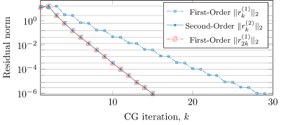
Figure 1: Illustration of Theorem 2.4

2.4 Contrast with related work

Our work is closely related to that of Xia [35, 38, 33], Li [22, 21], and Xin [39] (which concentrate however on the general, not sparse, case). In particular, our approach includes the double-sided scaling proposed in those works, as well as the implicit Schur compensation. The most significant difference is that we include an additional term $E$ in Eq. 10 (or $E_{2}$ in Eq. 14) after performing an explicit change of basis, which yields the quadratic approximation error. More precisely, the error in our approach is the $\mathcal{O}(\varepsilon^{2})$ error resulting from dropping the Schur complement update, and possibly an $\mathcal{O}(\varepsilon^{2})$ error in the elimination matrices. Thus, the overall approximation error is also $\mathcal{O}(\varepsilon^{2})$ while the other approaches have an $\mathcal{O}(\varepsilon)$ overall approximation error. Lastly, our methods do not require any special low-rank matrix formats, such as the HSS format used by some of the related approaches.

Most recently, Xia [34] used similar ideas, to improve the SIF algorithm for general (typically dense) SPD matrices [39]. Below, we use our methods to improve spaND [4], which is an algorithm for sparse matrices, related to, but different from SIF.

3 Hierarchical multilevel algorithm

Sparsified Nested Dissection (spaND) [4] is a hierarchical multilevel algorithm which repeatedly applies the first-order approximation scheme from Section 2.1. The first-order scheme can be easily replaced by the second-order schemes of Section 2.2. The spaND algorithm is guaranteed to complete on any SPD matrix. The result is an approximate factorization of $A$ which—under typical assumptions on the ranks of the fill-in blocks—can be computed in $\mathcal{O}(n\log(n))$ operations on a sparse matrix such as those arising from discretized PDEs. The resulting preconditioner can then be applied in $\mathcal{O}(n)$ operations.

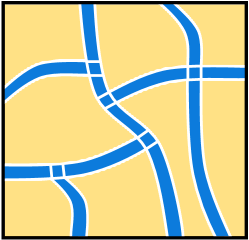
(a)

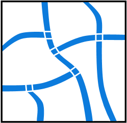
(b)

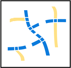
(c)

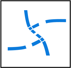
(d)

(e)

(f)

Figure 2: Visualization of the spaND algorithm. Interfaces are shown in blue and interiors in yellow. At each level, interiors only interact with (i.e., have edges connecting to) the neighboring interfaces. Interiors are first eliminated using the block Gaussian elimination. The remaining interfaces are then sparsified, which effectively eliminates (without fill-in) a number of variables from the system. The algorithm then proceeds to the next level and completes when the last level interface is eliminated.

We now describe the spaND algorithm, the details of which can be found in [4]. The algorithm is illustrated in Figure 2. It uses a multilevel ordering based on nested dissection. This ordering (called the spaND partitioning) is fully algebraic, that is, only the entries of $A$ are needed to define it (more specifically, the partitioning is defined on the adjacency graph of $A$). At each level, the unknowns are split into two groups of subsets: interiors and interfaces. The interfaces are small subsets that separate the interiors from each other. The precise definitions of interiors and interfaces can be found in [4].

Once the multilevel partitioning has been defined, one can perform the actual factorization, see Figure 2. At each level, the interiors are first eliminated using the block Gaussian elimination. The existence of interfaces limits the fill-in (Schur complement updates) arising during elimination. The fill-in matrix blocks (interactions between interfaces) are scaled as in Eq. 13, and afterward sparsified using the approximation scheme of Section 2, which reduces the size of the interfaces. At this point the algorithm proceeds to the next level. The algorithm completes when the variables in the last level are eliminated using the Cholesky decomposition. The repeated reduction in the sizes of the interfaces allows obtaining an efficient sparse algorithm.

The sparsification process is depicted in Fig. 3. After eliminating interiors, most of connections between interfaces are through fill-in blocks. Consider the interface $p$ in Fig. 3. The connections to its neighbors (collectively denoted by $w$) typically have the low-rank property. Using notation from Section 2 this means that the block $A_{12}:=A_{pw}$ has a quickly decaying spectrum. We can therefore sparsify $p$ as described in Section 2. The step described in Eq. 6 is a change of basis that splits the variables from $p$ into $c$ (the coarse variables) and $f$ (the fine variables). After the approximation step —Eq. 7 (first-order), Eq. 10 (full second-order), or Eq. 14 (superfine second-order)— has been applied, the variables from $f$ are disconnected from all other unknowns and effectively eliminated. This process does not introduce any fill-in. Algorithm 2 describes the spaND algorithm using a recursive formulation.

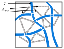
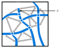
Figure 3: Illustration of the sparsification of a single interface $p$. The interactions between interfaces are conceptually shown in gray. The block $A_{pw}$ denotes the interactions of $p$ with the neighboring interfaces. Sparsifying $p$ splits it into $c$ (coarse variables) and $f$ (fine variables). Since $f$ is disconnected from all other interfaces, it is effectively eliminated ($f$ is represented by the piece of $p$ dropped in the picture above). This reduces the size of the interface without introducing any fill-in.

3.1 Obtaining the $E$ or $E_{2}$ matrix

To compute the $Q$ matrix from Eq. 6, spaND uses the column-pivoted rank-revealing QR (RRQR) which gives $A_{12}\Pi=QR$ where $\Pi$ is a permutation matrix. When using the first-order or the full second-order scheme, the decomposition can be stopped after $k$ steps, where $k$ is the smallest number such that $|R(k,k)|<\varepsilon|R(1,1)|$ (such relative criterion is typically chosen [4, 19, 18, 26, 7, 9]). At this point, we have

(28) $$A_{12}\Pi=\begin{pmatrix}Q_{c}&Q_{f}\end{pmatrix}R=\begin{pmatrix}Q_{c}&Q_{f}\end{pmatrix}\begin{pmatrix}R_{cc}&R_{cf}\\ 0&R_{ff}\\ \end{pmatrix}$$

where $Q_{c}$ has $k$ columns, and

$$E=Q_{f}^{\top}A_{12}=\begin{pmatrix}0&R_{ff}\end{pmatrix}\Pi^{\top}$$

Since both $R_{ff}$ and $\Pi$ are computed in the RRQR routine (see Section 4), obtaining $E$ involves a negligible additional cost. We also have $Q_{c}^{\top}A_{pw}=\begin{pmatrix}R_{cc}&R_{cf}\end{pmatrix}\Pi^{\top}$.

In the superfine second-order scheme, the decomposition is stopped later, with $k$ being the smallest number such that $|R(k,k)|<\varepsilon^{2}|R(1,1)|.$ At this point

(29) $$A_{12}\Pi=\begin{pmatrix}Q_{c}&Q_{f_{2}}&Q_{f_{1}}\end{pmatrix}R=\begin{pmatrix}Q_{c}&Q_{f_{2}}&Q_{f_{1}}\end{pmatrix}\begin{pmatrix}R_{cc}&R_{cf_{2}}&R_{cf_{1}}\\ 0&R_{f_{2}f_{2}}&R_{f_{2}f_{1}}\\ 0&0&R_{f_{1}f_{1}}\end{pmatrix}$$

We only need

$$E_{2}=Q_{f_{2}}^{\top}A_{12}=\begin{pmatrix}0&R_{f_{2}f_{2}}&R_{f_{2}f_{1}}\\ \end{pmatrix}\Pi^{\top}$$

Should $Q$ be computed separately, e.g., using randomized SVD, the matrix $E$ (or $E_{2}$) is obtained by performing the multiplication $Q_{f}^{\top}A_{12}$ (or $Q_{f_{2}}^{\top}A_{12}$). The (typically larger) multiplication $Q_{c}^{\top}A_{12}$ has to be performed regardless, and in our experience, is a small portion of the computations. Thus the second-order scheme involves only a minor additional computational cost also in this case.

0:  $A_{pw},0\leq\varepsilon\leq 1$

$$A_{pw}\Pi=\begin{cases}\begin{pmatrix}Q_{c}&Q_{f}\end{pmatrix}\begin{pmatrix}R_{cc}&R_{cf}\\ 0&R_{ff}\\ \end{pmatrix}&\parbox[t]{120.00018pt}{for the {first-order scheme} \\ or the {full second-order scheme}}\\ \begin{pmatrix}Q_{c}&Q_{f_{2}}&Q_{f_{1}}\end{pmatrix}\begin{pmatrix}R_{cc}&R_{cf_{2}}&R_{cf_{1}}\\ 0&R_{f_{2}f_{2}}&R_{f_{2}f_{1}}\\ 0&0&R_{f_{1}f_{1}}\end{pmatrix}&\parbox[t]{120.00018pt}{for the {superfine second-order scheme}}\end{cases}$$

where $\|R_{ff}\|=\mathcal{O}(\varepsilon)$, $\|R_{f_{1}f_{1}}\|=\mathcal{O}(\varepsilon^{2})$.

$$\widetilde{E}=\begin{cases}0&\mbox{for the {first-order scheme}}\\ E=Q_{f}^{\top}A_{pw}=\begin{pmatrix}0&R_{ff}\end{pmatrix}\Pi^{\top}&\parbox[t]{120.00018pt}{for the {full second-order scheme}}\\ \begin{pmatrix}0\\ E_{2}=Q_{f_{2}}^{\top}A_{pw}\end{pmatrix}=\begin{pmatrix}0\\ 0&R_{f_{2}f_{2}}&R_{f_{2}f_{1}}\\ \end{pmatrix}\Pi^{\top}&\parbox[t]{120.00018pt}{for the {superfine second-order scheme}}\end{cases}$$

  $Q_{c}^{\top}A_{pw}=\begin{pmatrix}R_{cc}&R_{cf}\end{pmatrix}\Pi^{\top}$

  return  $Q_{c},Q_{f},\widetilde{E},Q_{c}^{\top}A_{pw}$

Algorithm 1 Run column-pivoted QR; compute $E$ (or $E_{2}$), $Q_{c}$, $Q_{f}$ and $Q_{c}^{\top}A_{pw}$

3.2 Accuracy and relation between the factorization and solve

Notice that $\varepsilon>0$ controls the accuracy of the low-rank approximations and of the entire algorithm. Smaller value results in a more accurate factorization, which will take more time to compute. The resulting preconditioner will be more expensive to apply, but it will approximate $A^{-1}$ more accurately, resulting in fewer iterations in the solve phase (e.g., using Conjugate Gradient). We have $E\to 0$ as $\varepsilon\to 0$, in which case spaND becomes an exact block Cholesky factorization with a nested dissection ordering, and gives the exact solution. The optimal total runtime will likely be obtained long before, however, when the runtimes of the factorization and solve phases are more balanced.

0:  $A$, $0\leq\varepsilon\leq 1$

  spaND($A^{l}$, $l$)

  for all $s$ interior do {Eliminate interiors}

     Eliminate $s$ in one step of block Cholesky algorithm (with $A_{ss}=L_{s}L_{s}^{\top}$)

$$\begin{matrix}G_{s}\begin{pmatrix}A_{ss}&A_{sw}\\ A_{ws}&A_{ww}\end{pmatrix}G_{s}^{\top}=\begin{pmatrix}I&\\ &A_{ww}-A_{ws}A_{ss}^{-1}A_{sw}\end{pmatrix},&G_{s}=\begin{pmatrix}L_{s}^{-1}&\\ -A_{ws}L_{s}^{-\top}&I\end{pmatrix}\end{matrix}$$

  end for

  for all $p$ interface do {Scale interfaces}

     Scale $p$ using the Cholesky algorithm (with $A_{pp}=Z_{p}Z_{p}^{\top}$)

$$\begin{matrix}D_{p}\begin{pmatrix}A_{pp}&A_{pw}\\ A_{wp}&A_{ww}\end{pmatrix}D_{p}^{\top}=\begin{pmatrix}I&Z_{p}^{-1}A_{pw}\\ A_{wp}Z_{p}^{-\top}&A_{ww}\end{pmatrix},&D_{p}=\begin{pmatrix}Z_{p}^{-1}&\\ &I\end{pmatrix}\end{matrix}$$

  end for

  for all $p$ interface do {Sparsify interfaces}

     Run rank-revealing QR (Algorithm 1) to sparsify $p$

$$E_{p}Q_{p}^{\top}\begin{pmatrix}I&A_{pw}\\ A_{wp}&A_{ww}\end{pmatrix}Q_{p}E_{p}^{\top}\approx\begin{pmatrix}I&&\\ &I&Q_{c}^{\top}A_{pw}\\ &A_{wp}Q_{c}&A_{ww}\end{pmatrix}$$

$$\begin{matrix}Q_{p}=\begin{pmatrix}\begin{pmatrix}Q_{f}&Q_{c}\end{pmatrix}&\\ &I\end{pmatrix},&E_{p}=\begin{pmatrix}I&&\\ &I&\\ -\widetilde{E}^{\top}&&I\end{pmatrix}\end{matrix}$$

  end for

  $\begin{matrix}A^{l-1}=B_{l}A^{l}B_{l}^{\top},&B_{l}=\prod_{p}E_{p}^{l}Q_{p}^{l,\top}\prod_{p}D_{p}^{l}\prod_{s}G_{s}^{l}\end{matrix}$

  if $l>0$ then

     Recurse spaND($A^{l-1}_{P,P}$, $l-1$) where $P$ denotes the rows/columns corresponding to the non-yet-eliminated interfaces

  end if

Algorithm 2 The spaND algorithm in a recursive form. We assume that the special spaND partitioning [4] on $\ell\geq 1$ levels has been computed. The algorithm starts at level $l=\ell$, with $A^{\ell}=A$, and completes at $l=0$. The result is $M=L^{-\top}L^{-1}$ such that $L^{-1}AL^{-\top}\approx I$ with $L^{-1}=\prod_{l=0}^{\ell}\left(\prod_{p}(E_{p}^{l}Q_{p}^{\top,l})\prod_{p}D_{p}^{l}\prod_{s}G_{s}^{l}\right)$

4 Experimental results

We compare the preconditioners obtained when using the first- and second-order approximation schemes in the spaND algorithm. In all tested cases, the number of levels $\ell$ in the spaND partitioning is the closest integer to $\log_{2}(n/25),$ where $n$ is the number of rows in the tested matrix. We also skip the scaling and sparsification of interfaces in the first four levels of the algorithm, when the interfaces are still small. Thus, the only varying parameter is the accuracy $0\leq\varepsilon\leq 1$.

The spaND implementation is sequential and was written in C++, using BLAS and LAPACK [3] routines provided by Intel(R) MKL. In particular, the (early-stopping) rank-revealing QR factorization is implemented using the dlaqps routine from LAPACK. All experiments were run on CPUs with Intel(R) Xeon(R) E5-2640v4 (2.4GHz) processor with 128 GB RAM, always using a single thread.

The approximate inverse operator $M=L^{-\top}L^{-1}$ returned by spaND, is used in the preconditioned Conjugate Gradient (PCG) with a zero initial guess and convergence declared when the relative 2-norm of the residual falls below $10^{-10}$.

We further use the following notation:

• $n$ – is the number of unknowns (rows) of the given matrix $A$

• $nnz(A)$ – is the number of nonzero entries of $A$

• $n_{cg}$ – denotes the number of PCG iterations needed to converge

• $\mu$ – denotes the memory requirements needed to store the preconditioner, defined as $\mu:=nnz(L)/nnz(A)$

• $T_{f}$ – is the time needed to perform the spaND hierarchical factorization

• $T_{s}$ – is the time needed by PCG to converge

• $T_{t}$ – is the total time needed to solve the system, i.e., $T_{t}=T_{f}+T_{s}$

• $\Delta T_{s}$ – is the difference (in %) in the total runtime, when compared to the first-order scheme

All times are reported in seconds.

4.1 Low- and high-contrast Laplacians

We consider the elliptic equation

(30) $$\begin{matrix}\nabla(a(x)\cdot\nabla u(x))=f&\forall{x\in\Omega\in\left[0,1\right]^{2}},&u|_{\partial\Omega}=0\end{matrix}$$

discretized using the 5-point stencil method, on a square $d\times d$ grid. For $\rho\geq 1.0$, we define the $a(x)$ field as in [4, 9]. Namely, for $i,j=1,2,\ldots,d,$ we pick a random $\hat{a}_{ij}\in(0,1)$ from the uniform distribution, and convolve the resulting $d\times d$ field $\hat{a}$ with an isotropic Gaussian of standard deviation $\sigma=2$ to smooth the field out. We then quantize

(31) $$a_{ij}=\begin{cases}\rho&\mbox{if }\hat{a}_{ij}\geq 0.5\\ \rho^{-1}&\mbox{if }\hat{a}_{ij}<0.5.\end{cases}$$

Thus $\rho$ is a contrast parameter of the field. At $\rho=1.0$ we obtain the constant coefficient Poisson equation since then $a(x)\equiv 1.0$. At $\rho=100.0$ the contrast between coefficients is $\rho^{2}=10^{4}$. Examples of the coefficient fields are shown in Fig. 4. The condition number $\kappa(A)$ of the resulting matrix $A$ scales approximately as $\rho^{2}n.$

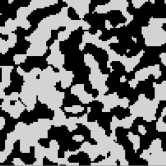
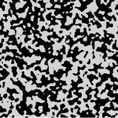
Figure 4: Examples of random coefficient fields used to define high-contrast Laplacians for $d=50$ (left) and $d=100$ (right).

4.1.1 Forward errors on eigenvectors

For the constant-coefficient case, i.e., when $\rho=1.0$, the unit-length eigenvectors of $A$ are known exactly. We therefore compute the forward errors $\|(I-MA)v_{\lambda}\|_{2}$ on selected unit-length eigenvectors $v_{\lambda}$. More precisely, for a given $p\in\{1,2,\ldots,d\}$ we consider the eigenvector corresponding to the function of the grid given by

$$x(i,j)=\sin\left(\frac{pi\pi}{d+1}\right)\sin\left(\frac{pj\pi}{d+1}\right)$$

which we normalize to obtain a unit-norm eigenvector $v_{\lambda_{p}}$. The corresponding eigenvalue is $\lambda_{p}=8\sin^{2}\left(\frac{p\pi}{2(d+1)}\right).$ In Figure 5 we plot the forward error as a function of the corresponding eigenvalue $\lambda$ for $d=1000$, i.e., for the $1000\times 1000$ grid. Because computing errors on all $10^{6}$ eigenvectors would be infeasible and difficult to plot, we consider $p\in\{\lfloor(5/4)^{k}\rfloor:k=0,1,2,\ldots\},\ p\leq d$. The corresponding eigenvalues fall in the whole range of magnitudes. For a given value of $\varepsilon$ parameter, the (full) second-order scheme is more accurate on all of the spectrum compared to the first-order scheme. The difference is particularly pronounced on the middle-to-high frequency eigenmodes. The accuracy on the lowest-frequency eigenmodes depends largely on the accuracy parameter $\varepsilon$.

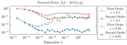
Figure 5: Forward errors on the unit-length eigenvectors of the 2D constant-coefficient Poisson equation. On the middle-to-high-frequency eigenmodes, the (full) second-order scheme with $\varepsilon=0.1$ is equally accurate as the first-order scheme with $\varepsilon=0.01$.

4.1.2 Halved PCG iteration counts and improved total timings

We perform a scaling study on square grids of increasing sizes for $\rho=1.0$ (constant-coefficient field) and $\rho=100.0$ (high-contrast field). The problems are refined by doubling the size of the grid in each dimension. In each case we solve the system $Ax=b$ where $b$ is a vector of ones. The results for $\varepsilon=0.01$ and $\varepsilon=0.001$ are shown in Table 1. For both values of $\rho$, and all tested grid sizes, we consistently observe that the number of iterations needed for convergence is halved when using the full second-order scheme as compared to the first-order scheme, with approximately the same factorization time, resulting in improved total timings.

$\bf\rho=1.0$ (no contrast)					First Order			Second Order
$d$	$n=d^{2}$	$\varepsilon$	$\mu$	$n_{cg}$	$T_{f}[s]$	$T_{s}[s]$	$T_{t}[s]$	$\mu$	$n_{cg}$	$T_{f}[s]$	$T_{s}[s]$	$T_{t}[s]$
400	0.16M	0.01	7.8	9	0.5	0.6	1.1	8.6	5	0.4	0.3	0.6
800	0.64M	0.01	7.7	11	2.1	2.9	5.1	8.5	6	1.7	1.5	3.2
1600	2.56M	0.01	7.7	16	8.8	17.4	26.2	8.5	8	10.1	10.6	20.7
3200	10.2M	0.01	7.7	22	37.1	103.9	141.0	8.5	11	35.9	54.8	90.7
6400	41.0M	0.01	7.6	34	145.0	666.9	811.9	8.4	17	150.0	346.1	496.1
400	0.16M	0.001	8.1	5	0.5	0.3	0.8	8.9	3	0.4	0.2	0.6
800	0.64M	0.001	8.0	6	1.8	1.4	3.1	8.8	3	2.0	0.9	2.9
1600	2.56M	0.001	8.0	7	7.5	6.3	13.8	8.9	4	9.3	4.9	14.2
3200	10.2M	0.001	8.0	8	35.6	35.8	71.4	8.8	4	35.8	19.9	55.8
6400	41.0M	0.001	7.9	10	167.6	215.7	383.3	8.7	5	152.4	115.8	268.2
$\bf\rho=100.0$ (high contrast)					First Order			Second Order
$d$	$n=d^{2}$	$\varepsilon$	$\mu$	$n_{cg}$	$T_{f}[s]$	$T_{s}[s]$	$T_{t}[s]$	$\mu$	$n_{cg}$	$T_{f}[s]$	$T_{s}[s]$	$T_{t}[s]$
400	0.16M	0.01	7.6	15	0.5	0.9	1.4	8.3	7	0.5	0.4	0.9
800	0.64M	0.01	7.5	22	2.1	5.7	7.8	8.3	11	1.8	2.9	4.7
1600	2.56M	0.01	7.6	28	8.7	28.2	36.9	8.3	13	7.6	13.7	21.3
3200	10.2M	0.01	7.5	46	33.6	197.0	230.6	8.3	22	29.6	90.4	120.0
6400	41.0M	0.01	7.5	82	140.6	1599.0	1739.6	8.2	38	142.6	748.5	891.1
400	0.16M	0.001	7.8	8	0.4	0.4	0.8	8.5	4	0.5	0.3	0.7
800	0.64M	0.001	7.7	9	1.8	2.2	4.0	8.5	5	1.8	1.2	3.0
1600	2.56M	0.001	7.8	10	7.5	9.1	16.6	8.5	5	7.4	5.0	12.5
3200	10.2M	0.001	7.7	12	38.4	53.8	92.2	8.5	6	35.3	29.4	64.7
6400	41.0M	0.001	7.7	16	144.9	316.4	461.3	8.5	8	154.7	182.9	337.6

Table 1: Scaling study on 2D Laplacians. Second-order scheme consistently halves the number of PCG iterations for approximately the same factorization time.

4.2 SuiteSparse matrices

To test the efficiencies of the new approximation schemes in practice, we run the spaND algorithm on all SPD matrices from the University of Florida sparse matrix collection [8] (SuiteSparse), with at least 500,000 rows. We run spaND with the first-order scheme, the full second-order scheme, and the superfine second-order scheme. We test four values of the accuracy parameter $\varepsilon=0.2,0.1,0.05,0.01$. At $\varepsilon=0.01,$ PCG converges in a small number of iterations on all tested matrices. As mentioned above, $\varepsilon$ is the only varying parameter.

In each case, we solve the system $A^{\prime}x=b^{\prime}$ where $A^{\prime}=D^{-\frac{1}{2}}AD^{-\frac{1}{2}}$, $b^{\prime}=D^{-\frac{1}{2}}b$ with $D$ being the diagonal of $A$, and $b$ a vector of ones. Such diagonal prescaling is recommended [31, 10], when solving structural problems which are among the most challenging test cases.

4.2.1 Halved PCG counts and improved solve times

Similar as in the Laplace scaling study, for a given accuracy parameter $\varepsilon,$ the number of PCG iterations needed for convergence is almost exactly halved when using the full second-order scheme, across all tested cases. This is also true for the superfine second-order scheme, on almost all of the problems. Example aggregate results are shown in Figure 6.

For a given $\varepsilon$ parameter the preconditioners using the new second-order schemes are more expensive to apply. However, the increase in memory requirement (proportional to the cost of applying the preconditioner), is moderate, never exceeding 100%, as shown in Figure 8. As a result, the time needed for convergence of PCG is still significantly reduced in all cases. This is shown in Figure 9.

4.2.2 Squeezed convergence plots

In Figure 7 we show example plots of the 2-norm error decay in the PCG algorithm. We observe that, for a given problem and accuracy parameter, the behavior of the residual $\|A^{\prime}x_{k}-b^{\prime}\|/\|b^{\prime}\|$ as a function of $k$, when using the full second-order scheme, is approximately the same as the behavior of $\|A^{\prime}x_{2k}-b^{\prime}\|/\|b^{\prime}\|$ when using the first-order scheme. As a result, the plot when using the full second-order scheme is squeezed compared to the plot when using the first-order scheme, but retains its general shape. This behavior is approximately the same as in the conclusion of Theorem 2.4. We note here that we observed the same behavior of convergence plots when the right-hand sides were chosen at random.

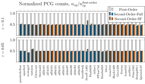
Figure 6: Normalized PCG iteration counts on all tested SuiteSparse SPD matrices with at least 500,000 rows. For a given matrix and accuracy parameter $\varepsilon$, the number of iterations needed for convergence using the second-order schemes, is almost exactly halved compared to the first-order scheme.

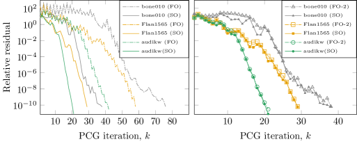
Figure 7: Error decay in PCG preconditioned with spaND (accuracy $\varepsilon=0.01$), for selected SuiteSparse matrices. On the left, we compare the convergence using the first-order scheme (FO) and the full second-order scheme (SO). On the right, for each iteration $k$ we compare the residual obtained when using the full second-order scheme (SO) with the residual at the $2k$-th iteration when using the first-order scheme (FO-2).

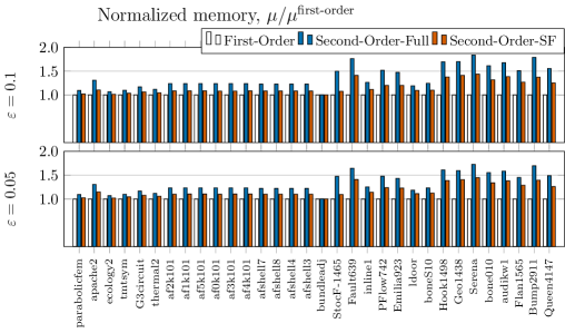
Figure 8: Normalized memory requirements for the SuiteSparse matrices. The increase in memory requirements using the second-order schemes, never exceeds 100%. When using the superfine second-order scheme, it never exceeds 50%.

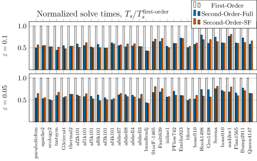
Figure 9: Normalized solve times for the SuiteSparse matrices. For a given matrix and accuracy parameter $\varepsilon$, the time needed for convergence of PCG is significantly reduced when using the second-order schemes.

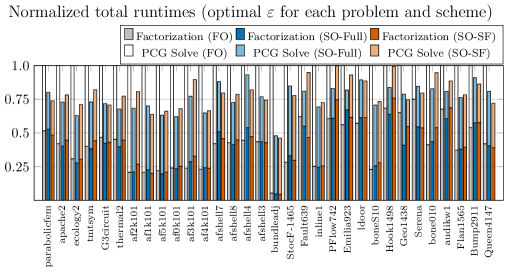
Figure 10: Normalized total runtimes ($T_{t}/T_{t}^{\text{first-order}}=T_{f}/T_{t}^{\text{first-order}}+T_{s}/T_{t}^{\text{first-order}}$) for the SuiteSprase matrices. For each problem, and each tested scheme, the optimal corresponding $\varepsilon$ was chosen, from the four tested ones ($\varepsilon=0.2,0.1,0.05,0.01$). Second-order schemes improve the total runtimes in all tested cases.

4.2.3 Improved total timings

Since for a given $\varepsilon$ parameter the factorization phase of spaND involves little additional computations when using the second-order schemes, the total runtimes should also be reduced. In Figure 10, for each tested matrix, and each scheme, we show the best runtime from amongst the four tested accuracy parameters $\varepsilon$, split into the factorization and solve (PCG iteration) phases (full data can be found in Appendix B). We observe improvements in the optimal total runtime in all tested cases when using the new second-order schemes.

Notice that a significantly shorter solve time $T_{s}$ for the same accuracy parameter $\varepsilon$, may mean that—from the standpoint of optimizing the total runtime—the factorization is too accurate. Therefore one can expect that the optimal total runtime when using the second-order schemes will be obtained for a larger accuracy parameter $\varepsilon$, than when using the first-order scheme. We observe this for a number of test cases (for example Geo1436 or Serena, see also Appendix B).

4.3 Differences between the two second-order scheme variants

For the same accuracy parameter $\varepsilon$, on almost all tested problems, the superfine second-order scheme and the full second-order scheme resulted in nearly the same PCG iteration counts. The superfine second-order scheme preconditioner has lower memory requirements than the full second-order scheme preconditioner, and is cheaper to apply. This may translate to savings in the solution phase. The rank-revealing QR has to be computed down to $\varepsilon^{2}$ accuracy, however, which may make the factorization phase more expensive. Both second-order scheme variants performed competitively in our test cases.

5 Conclusions

We introduced a second-order accurate approach to sparsifying the numerically low-rank blocks in the approximate hierarchical factorizations of sparse symmetric positive definite matrices. Similar to the standard first-order approach, we apply orthogonal matrices defined by the rank-revealing decomposition of the given off-diagonal block, so that interactions of many variables become small, and are subsequently dropped. However, the new approach also includes additional terms that approximately eliminate these variables. As a result, the norm of the overall error depends quadratically, as opposed to linearly, on the norm of the error in the low-rank approximation of the given block.

Numerical analysis of the resulting two-level preconditioners, as well as numerical experiments, show clear improvements provided by the new method. In particular, the analysis suggests that the number of Conjugate Gradient iterations should be halved for any given accuracy parameter. Consistent with this, when incorporated into the spaND algorithm [4], for any given accuracy, the new approach results in a reduction of iteration counts by almost exactly half, on a wide range of SPD problems. The new approach involves little additional computations in the factorization phase, and improves the total runtimes of spaND.

Beside spaND, other solvers based on hierarchical low-rank structures can benefit from our results when applied to sparse matrices. In particular, we considered only factorizations sparsifying all off-diagonal blocks but the second-order scheme can be similarly defined for algorithms distinguishing neighboring and well-separated interactions, such as [29, 26, 25, 7]. Also, the sparsification approach that improves accuracy on the chosen near-kernel subspace, as in [19], can be applied basically without modifications. Lastly, the new approach can be expected to work optimally for a lower accuracy parameter, as observed on some test problems. This should improve the parallel properties of hierarchical solvers because a larger portion of computations is then performed on small blocks in the initial levels of the algorithm.

Appendix A Proof of Theorem 2.4

Proof A.1.

Denote $F=I-C^{\top}C.$ We have $A_{1}\begin{pmatrix}b_{1}\\ b_{2}\end{pmatrix}=\begin{pmatrix}Cb_{2}+b_{1}\\ b_{2}\end{pmatrix}$. We also have

$$\begin{pmatrix}-Cb_{2}+b_{1}\\ b_{2}\end{pmatrix}=-\begin{pmatrix}Cb_{2}+b_{1}\\ b_{2}\end{pmatrix}+2\begin{pmatrix}b_{1}\\ b_{2}\end{pmatrix}$$

and

(32) $$A_{1}\begin{pmatrix}-Cb_{2}+b_{1}\\ b_{2}\end{pmatrix}=\begin{pmatrix}b_{1}\\ Fb_{2}\end{pmatrix}$$

By iterating this (with $Fb_{2}$ in place of $b_{2}$), we have that one particular sequence of vectors defining the Krylov subspaces for $(A_{1},b)$, is given by:

(33) $$\mathcal{K}(A_{1},b)$$

$$=\Big{\{}\begin{pmatrix}b_{1}\\ b_{2}\end{pmatrix},\begin{pmatrix}-Cb_{2}+b_{1}\\ b_{2}\end{pmatrix},\begin{pmatrix}b_{1}\\ Fb_{2}\end{pmatrix},\begin{pmatrix}-CFb_{2}+b_{1}\\ Fb_{2}\end{pmatrix},\begin{pmatrix}b_{1}\\ F^{2}b_{2}\end{pmatrix},\begin{pmatrix}-CF^{2}b_{2}+b_{1}\\ F^{2}b_{2}\end{pmatrix},\dots\Big{\}}$$

An analogous sequence for $(A_{2},b)$ is given by

$$\mathcal{K}(A_{2},b)=\Big{\{}\begin{pmatrix}b_{1}\\ b_{2}\end{pmatrix},\begin{pmatrix}b_{1}\\ Fb_{2}\end{pmatrix},\begin{pmatrix}b_{1}\\ F^{2}b_{2}\end{pmatrix},\dots\Big{\}}$$

There exist coefficients $\alpha_{i}$, for $0\leq i\leq k-1,$ such that the Conjugate Gradient solution to $A_{2}x=b$ at the $k$-th iteration, is given by:

$$x^{(2)}_{k}=\sum_{i=0}^{k-1}\alpha_{i}\begin{pmatrix}b_{1}\\ F^{i}b_{2}\end{pmatrix}$$

The residual then equals

$$r^{(2)}_{k}=b-A_{2}\sum_{i=0}^{k-1}\alpha_{i}\begin{pmatrix}b_{1}\\ F^{i}b_{2}\end{pmatrix}=b-\sum_{i=0}^{k-1}\alpha_{i}\begin{pmatrix}b_{1}\\ F^{i+1}b_{2}\end{pmatrix}$$

From the optimality conditions of the Conjugate Gradient solution, we have

(34) $$r^{(2)}_{k}=b-\sum_{i=0}^{k-1}\alpha_{i}\begin{pmatrix}b_{1}\\ F^{i+1}b_{2}\end{pmatrix}\perp\langle\Big{\{}\begin{pmatrix}b_{1}\\ F^{i}b_{2}\end{pmatrix}\Big{\}}_{i=0}^{k-1}\rangle$$

Define:

$$s:=b-A_{1}\sum_{i=0}^{k-1}\alpha_{i}\begin{pmatrix}-CF^{i}b_{2}+b_{1}\\ F^{i}b_{2}\end{pmatrix}$$

From 32 and 34, we have:

(35) $$s=b-\sum_{i=0}^{k-1}\alpha_{i}\begin{pmatrix}b_{1}\\ F^{i+1}b_{2}\end{pmatrix}=r_{k}^{(2)}\perp\langle\Big{\{}\begin{pmatrix}b_{1}\\ F^{i}b_{2}\end{pmatrix}\Big{\}}_{i=0}^{k-1}\rangle$$

We now show that also

$$s\perp\langle\Big{\{}\begin{pmatrix}-CF^{i}b_{2}+b_{1}\\ F^{i}b_{2}\end{pmatrix}\Big{\}}_{i=0}^{k-1}\rangle$$

From 35 it suffices to show that

$$s=b-\sum_{i=0}^{k-1}\alpha_{i}\begin{pmatrix}b_{1}\\ F^{i+1}b_{2}\end{pmatrix}\perp\langle\Big{\{}\begin{pmatrix}-CF^{i}b_{2}\\ 0\end{pmatrix}\Big{\}}_{i=0}^{k-1}\rangle$$

However, this holds, because for any $0\leq i\leq k-1$

$$s^{\top}\begin{pmatrix}-CF^{i}b_{2}\\ 0\end{pmatrix}=\Big{(}\sum_{j=0}^{k-1}{\alpha_{j}}-1\Big{)}b_{1}^{\top}CF^{i}b_{2}=0$$

which follows from the assumption that $b_{1}^{\top}C=0$. This means that $s$ is orthogonal to the $2k$-th Krylov subspace for $A_{1}$, and therefore, again from the optimality conditions

$$x^{(1)}_{2k}:=\sum_{i=0}^{k-1}\alpha_{i}\begin{pmatrix}-CF^{i}b_{2}+b_{1}\\ F^{i}b_{2}\end{pmatrix}$$

is the solution to $A_{1}x=b$ produced at the $2k$-th iteration, and

$$r^{(1)}_{2k}=s=r_{k}^{(2)}$$

Appendix B Tables with runs for optimal $\varepsilon$

For each tested matrix from the SuiteSparse collection, and each sparsification scheme, we show the run with optimal $\varepsilon$ (from among the four tested, $\varepsilon=0.2,0.1,0.05,0.01$) in terms of the total runtime. Some of the matrices (almost identical to already shown), were omitted.

Matrix	$n$	$nnz(A)$	Order	$\varepsilon$	$\mu$	$n_{cg}$	$T_{f}[s]$	$T_{s}[s]$	$T_{t}[s]$	$\Delta T_{t}$
parabolicfem	$5.3\cdot 10^{5}$	$3.7\cdot 10^{6}$	First	0.01	8.9	10	2.9	2.7	5.6	–
	$5.3\cdot 10^{5}$	$3.7\cdot 10^{6}$	Sec-Full	0.01	9.8	5	3.0	1.5	4.5	-19.9%
	$5.3\cdot 10^{5}$	$3.7\cdot 10^{6}$	Sec-SF	0.01	9.2	5	2.7	1.4	4.1	-26.2%
apache2	$7.2\cdot 10^{5}$	$4.8\cdot 10^{6}$	First	0.01	17.0	24	11.9	16.5	28.4	–
	$7.2\cdot 10^{5}$	$4.8\cdot 10^{6}$	Sec-Full	0.01	21.9	12	11.5	9.3	20.7	-27.1%
	$7.2\cdot 10^{5}$	$4.8\cdot 10^{6}$	Sec-SF	0.01	20.2	12	12.7	9.6	22.2	-21.8%
ecology2	$1.0\cdot 10^{6}$	$5.0\cdot 10^{6}$	First	0.01	10.3	17	2.5	5.7	8.2	–
	$1.0\cdot 10^{6}$	$5.0\cdot 10^{6}$	Sec-Full	0.01	11.0	8	2.3	2.9	5.1	-37.1%
	$1.0\cdot 10^{6}$	$5.0\cdot 10^{6}$	Sec-SF	0.01	10.6	9	2.5	3.3	5.8	-29.0%
tmtsym	$7.3\cdot 10^{5}$	$5.1\cdot 10^{6}$	First	0.01	6.9	20	5.3	7.9	13.2	–
	$7.3\cdot 10^{5}$	$5.1\cdot 10^{6}$	Sec-Full	0.01	7.6	10	5.0	4.6	9.6	-27.0%
	$7.3\cdot 10^{5}$	$5.1\cdot 10^{6}$	Sec-SF	0.01	7.3	10	5.8	5.0	10.8	-17.9%
G3circuit	$1.6\cdot 10^{6}$	$7.7\cdot 10^{6}$	First	0.01	12.9	14	12.2	14.0	26.2	–
	$1.6\cdot 10^{6}$	$7.7\cdot 10^{6}$	Sec-Full	0.01	14.9	7	11.1	7.7	18.8	-28.3%
	$1.6\cdot 10^{6}$	$7.7\cdot 10^{6}$	Sec-SF	0.01	14.1	7	11.3	7.3	18.6	-29.3%
thermal2	$1.2\cdot 10^{6}$	$8.6\cdot 10^{6}$	First	0.01	6.3	16	10.2	12.4	22.6	–
	$1.2\cdot 10^{6}$	$8.6\cdot 10^{6}$	Sec-Full	0.01	7.0	8	9.0	6.3	15.3	-32.3%
	$1.2\cdot 10^{6}$	$8.6\cdot 10^{6}$	Sec-SF	0.01	6.7	8	10.1	7.4	17.5	-22.7%

Table 2: (Part 1/3) SuiteSparse SPD matrices: best runs in terms of the total runtime.

Matrix	$n$	$nnz(A)$	Order	$\varepsilon$	$\mu$	$n_{cg}$	$T_{f}[s]$	$T_{s}[s]$	$T_{t}[s]$	$\Delta T_{t}$
afshell8	$5.0\cdot 10^{5}$	$1.8\cdot 10^{7}$	First	0.01	3.9	16	3.9	5.0	8.9	–
	$5.0\cdot 10^{5}$	$1.8\cdot 10^{7}$	Sec-Full	0.01	4.7	8	3.9	3.0	6.8	-23.1%
	$5.0\cdot 10^{5}$	$1.8\cdot 10^{7}$	Sec-SF	0.01	4.4	8	3.8	2.8	6.6	-25.7%
bundleadj	$5.1\cdot 10^{5}$	$2.0\cdot 10^{7}$	First	0.01	2.3	86	0.8	13.4	14.1	–
	$5.1\cdot 10^{5}$	$2.0\cdot 10^{7}$	Sec-Full	0.01	2.3	42	0.7	6.1	6.8	-52.0%
	$5.1\cdot 10^{5}$	$2.0\cdot 10^{7}$	Sec-SF	0.01	2.3	45	0.6	5.9	6.5	-53.8%
StocF-1465	$1.5\cdot 10^{6}$	$2.1\cdot 10^{7}$	First	0.01	20.7	122	137.3	348.3	485.6	–
	$1.5\cdot 10^{6}$	$2.1\cdot 10^{7}$	Sec-Full	0.01	29.9	58	160.2	251.8	412.1	-15.1%
	$1.5\cdot 10^{6}$	$2.1\cdot 10^{7}$	Sec-SF	0.01	24.1	61	143.7	234.0	377.7	-22.2%
Fault639	$6.4\cdot 10^{5}$	$2.9\cdot 10^{7}$	First	0.05	14.1	44	106.9	65.6	172.5	–
	$6.4\cdot 10^{5}$	$2.9\cdot 10^{7}$	Sec-Full	0.05	23.1	21	94.9	44.7	139.6	-19.1%
	$6.4\cdot 10^{5}$	$2.9\cdot 10^{7}$	Sec-SF	0.1	16.3	46	80.3	83.2	163.5	-5.2%
af5k101	$5.0\cdot 10^{5}$	$1.8\cdot 10^{7}$	First	0.01	3.9	40	3.8	12.8	16.7	–
	$5.0\cdot 10^{5}$	$1.8\cdot 10^{7}$	Sec-Full	0.01	4.8	19	4.0	6.8	10.8	-35.2%
	$5.0\cdot 10^{5}$	$1.8\cdot 10^{7}$	Sec-SF	0.01	4.4	20	4.0	7.1	11.1	-33.6%
inline1	$5.0\cdot 10^{5}$	$3.7\cdot 10^{7}$	First	0.01	3.7	72	12.8	38.0	51.2	–
	$5.0\cdot 10^{5}$	$3.7\cdot 10^{7}$	Sec-Full	0.01	4.5	33	12.5	22.7	35.2	-30.7%
	$5.0\cdot 10^{5}$	$3.7\cdot 10^{7}$	Sec-SF	0.01	4.3	33	12.9	23.9	36.8	-27.5%
PFlow742	$7.4\cdot 10^{5}$	$3.7\cdot 10^{7}$	First	0.01	6.9	22	39.8	25.9	65.7	–
	$7.4\cdot 10^{5}$	$3.7\cdot 10^{7}$	Sec-Full	0.01	9.7	10	40.0	14.5	54.5	-17.0%
	$7.4\cdot 10^{5}$	$3.7\cdot 10^{7}$	Sec-SF	0.01	8.9	10	48.9	16.5	65.4	-0.4%
Emilia923	$9.2\cdot 10^{5}$	$4.1\cdot 10^{7}$	First	0.1	17.6	80	199.1	156.6	355.7	–
	$9.2\cdot 10^{5}$	$4.1\cdot 10^{7}$	Sec-Full	0.05	27.7	17	238.4	52.5	291.0	-18.2%
	$9.2\cdot 10^{5}$	$4.1\cdot 10^{7}$	Sec-SF	0.1	21.1	41	218.6	112.1	330.7	-7.0%
ldoor	$9.5\cdot 10^{5}$	$4.7\cdot 10^{7}$	First	0.01	2.8	9	7.4	5.6	13.0	–
	$9.5\cdot 10^{5}$	$4.7\cdot 10^{7}$	Sec-Full	0.01	3.3	5	7.9	3.7	11.6	-10.7%
	$9.5\cdot 10^{5}$	$4.7\cdot 10^{7}$	Sec-SF	0.01	3.1	5	8.0	3.5	11.5	-11.5%
boneS10	$9.1\cdot 10^{5}$	$5.5\cdot 10^{7}$	First	0.01	4.0	64	16.5	55.3	71.8	–
	$9.1\cdot 10^{5}$	$5.5\cdot 10^{7}$	Sec-Full	0.01	4.8	31	18.3	32.4	50.7	-29.3%
	$9.1\cdot 10^{5}$	$5.5\cdot 10^{7}$	Sec-SF	0.01	4.5	31	20.0	32.6	52.6	-26.7%
Hook1498	$1.5\cdot 10^{6}$	$6.1\cdot 10^{7}$	First	0.01	13.7	34	209.6	97.0	306.5	–
	$1.5\cdot 10^{6}$	$6.1\cdot 10^{7}$	Sec-Full	0.01	20.1	17	195.4	61.1	256.4	-16.3%
	$1.5\cdot 10^{6}$	$6.1\cdot 10^{7}$	Sec-SF	0.01	18.4	17	232.5	71.9	304.4	-0.7%
Geo1438	$1.4\cdot 10^{6}$	$6.3\cdot 10^{7}$	First	0.05	15.0	39	263.6	141.9	405.6	–
	$1.4\cdot 10^{6}$	$6.3\cdot 10^{7}$	Sec-Full	0.1	20.9	37	166.1	153.5	319.6	-21.2%
	$1.4\cdot 10^{6}$	$6.3\cdot 10^{7}$	Sec-SF	0.05	21.1	19	221.9	80.7	302.6	-25.4%
Serena	$1.4\cdot 10^{6}$	$6.5\cdot 10^{7}$	First	0.05	13.7	31	292.1	97.7	389.8	–
	$1.4\cdot 10^{6}$	$6.5\cdot 10^{7}$	Sec-Full	0.1	20.7	25	212.1	117.4	329.5	-15.5%
	$1.4\cdot 10^{6}$	$6.5\cdot 10^{7}$	Sec-SF	0.1	16.1	26	209.2	101.3	310.5	-20.3%
bone010	$9.9\cdot 10^{5}$	$7.2\cdot 10^{7}$	First	0.01	8.5	76	104.6	149.0	253.6	–
	$9.9\cdot 10^{5}$	$7.2\cdot 10^{7}$	Sec-Full	0.01	12.2	38	110.4	99.4	209.9	-17.2%
	$9.9\cdot 10^{5}$	$7.2\cdot 10^{7}$	Sec-SF	0.01	11.1	36	136.7	103.3	240.0	-5.4%

Table 3: (Part 2/3) SuiteSparse SPD matrices: best runs in terms of the total runtime.

Matrix	$n$	$nnz(A)$	Order	$\varepsilon$	$\mu$	$n_{cg}$	$T_{f}[s]$	$T_{s}[s]$	$T_{t}[s]$	$\Delta T_{t}$
audikw1	$9.4\cdot 10^{5}$	$7.8\cdot 10^{7}$	First	0.01	9.6	42	219.9	110.6	330.5	–
	$9.4\cdot 10^{5}$	$7.8\cdot 10^{7}$	Sec-Full	0.01	13.8	21	195.5	65.3	260.8	-21.1%
	$9.4\cdot 10^{5}$	$7.8\cdot 10^{7}$	Sec-SF	0.01	12.7	21	221.2	64.5	285.7	-13.5%
Flan1565	$1.6\cdot 10^{6}$	$1.2\cdot 10^{8}$	First	0.01	7.0	58	107.2	180.4	287.6	–
	$1.6\cdot 10^{6}$	$1.2\cdot 10^{8}$	Sec-Full	0.01	9.4	29	108.9	110.5	219.4	-23.7%
	$1.6\cdot 10^{6}$	$1.2\cdot 10^{8}$	Sec-SF	0.01	8.8	29	113.3	111.8	225.1	-21.7%
Bump2911	$2.9\cdot 10^{6}$	$1.3\cdot 10^{8}$	First	0.1	15.4	89	797.3	681.5	1478.8	–
	$2.9\cdot 10^{6}$	$1.3\cdot 10^{8}$	Sec-Full	0.1	27.5	39	849.3	495.3	1344.6	-9.1%
	$2.9\cdot 10^{6}$	$1.3\cdot 10^{8}$	Sec-SF	0.1	21.1	42	851.2	424.3	1275.5	-13.7%
Queen4147	$4.1\cdot 10^{6}$	$3.3\cdot 10^{8}$	First	0.2	9.5	110	842.0	1169.5	2011.5	–
	$4.1\cdot 10^{6}$	$3.3\cdot 10^{8}$	Sec-Full	0.2	15.7	49	812.8	812.6	1625.4	-19.2%
	$4.1\cdot 10^{6}$	$3.3\cdot 10^{8}$	Sec-SF	0.2	11.6	57	786.6	661.9	1448.5	-28.0%

Table 4: (Part 3/3) SuiteSparse SPD matrices: best runs in terms of the total runtime.

References

• [1] P. Amestoy, C. Ashcraft, O. Boiteau, A. Buttari, J.-Y. L’Excellent, and C. Weisbecker, Improving multifrontal methods by means of block low-rank representations, SIAM Journal on Scientific Computing, 37 (2015), pp. A1451–A1474.
• [2] A. Aminfar, S. Ambikasaran, and E. Darve, A fast block low-rank dense solver with applications to finite-element matrices, Journal of Computational Physics, 304 (2016), pp. 170–188.
• [3] E. Anderson, Z. Bai, C. Bischof, S. Blackford, J. Dongarra, J. Du Croz, A. Greenbaum, S. Hammarling, A. McKenney, and D. Sorensen, LAPACK Users’ guide, vol. 9, Siam, 1999.
• [4] L. Cambier, C. Chen, E. G. Boman, S. Rajamanickam, R. S. Tuminaro, and E. Darve, An algebraic sparsified nested dissection algorithm using low-rank approximations, SIAM Journal on Matrix Analysis and Applications, 41 (2020), pp. 715–746.
• [5] S. Chandrasekaran, M. Gu, X. S. Li, and J. Xia, Superfast multifrontal method for structured linear systems of equations, preprint, (2007).
• [6] C. Chen, L. Cambier, E. G. Boman, S. Rajamanickam, R. S. Tuminaro, and E. Darve, A robust hierarchical solver for ill-conditioned systems with applications to ice sheet modeling, Journal of Computational Physics, 396 (2019), pp. 819–836.
• [7] C. Chen, H. Pouransari, S. Rajamanickam, E. G. Boman, and E. Darve, A distributed-memory hierarchical solver for general sparse linear systems, Parallel Computing, 74 (2018), pp. 49–64.
• [8] T. A. Davis and Y. Hu, The university of florida sparse matrix collection, ACM Transactions on Mathematical Software (TOMS), 38 (2011), pp. 1–25.
• [9] J. Feliu-Fabà, K. L. Ho, and L. Ying, Recursively preconditioned hierarchical interpolative factorization for elliptic partial differential equations, arXiv preprint arXiv:1808.01364, (2018).
• [10] A. Franceschini, N. Castelletto, and M. Ferronato, Block preconditioning for fault/fracture mechanics saddle-point problems, Computer Methods in Applied Mechanics and Engineering, 344 (2019), pp. 376–401.
• [11] A. George, Nested dissection of a regular finite element mesh, SIAM Journal on Numerical Analysis, 10 (1973), pp. 345–363.
• [12] P. Ghysels, X. S. Li, F.-H. Rouet, S. Williams, and A. Napov, An efficient multicore implementation of a novel hss-structured multifrontal solver using randomized sampling, SIAM Journal on Scientific Computing, 38 (2016), pp. S358–S384.
• [13] A. Gillman and P.-G. Martinsson, A direct solver with o(n) complexity for variable coefficient elliptic pdes discretized via a high-order composite spectral collocation method, SIAM Journal on Scientific Computing, 36 (2014), pp. A2023–A2046.
• [14] G. H. Golub and C. F. Van Loan, Matrix computations, vol. 3, JHU press, 2012.
• [15] L. Grasedyck, W. Hackbusch, and R. Kriemann, Performance of h-lu preconditioning for sparse matrices, Computational Methods in Applied Mathematics Comput. Methods Appl. Math., 8 (2008), pp. 336–349.
• [16] L. Grasedyck, R. Kriemann, and S. Le Borne, Domain decomposition based $\mathcal{H}$-lu preconditioning, Numerische Mathematik, 112 (2009), pp. 565–600.
• [17] M. R. Hestenes, E. Stiefel, et al., Methods of conjugate gradients for solving linear systems, Journal of research of the National Bureau of Standards, 49 (1952), pp. 409–436.
• [18] K. L. Ho and L. Ying, Hierarchical interpolative factorization for elliptic operators: differential equations, Communications on Pure and Applied Mathematics, 69 (2016), pp. 1415–1451.
• [19] B. Klockiewicz and E. Darve, Sparse hierarchical preconditioners using piecewise smooth approximations of eigenvectors, arXiv preprint arXiv:1907.03406, (2019).
• [20] W. Y. Kong, J. Bremer, and V. Rokhlin, An adaptive fast direct solver for boundary integral equations in two dimensions, Applied and Computational Harmonic Analysis, 31 (2011), pp. 346–369.
• [21] S. Li, M. Gu, and L. Cheng, Fast structured lu factorization for nonsymmetric matrices, Numerische Mathematik, 127 (2014), pp. 35–55.
• [22] S. Li, M. Gu, C. J. Wu, and J. Xia, New efficient and robust hss cholesky factorization of spd matrices, SIAM Journal on Matrix Analysis and Applications, 33 (2012), pp. 886–904.
• [23] Y. Li and L. Ying, Distributed-memory hierarchical interpolative factorization, Research in the Mathematical Sciences, 4 (2017), p. 12.
• [24] R. J. Lipton, D. J. Rose, and R. E. Tarjan, Generalized nested dissection, SIAM journal on numerical analysis, 16 (1979), pp. 346–358.
• [25] V. Minden, K. L. Ho, A. Damle, and L. Ying, A recursive skeletonization factorization based on strong admissibility, Multiscale Modeling & Simulation, 15 (2017), pp. 768–796.
• [26] H. Pouransari, P. Coulier, and E. Darve, Fast hierarchical solvers for sparse matrices using extended sparsification and low-rank approximation, SIAM Journal on Scientific Computing, 39 (2017), pp. A797–A830.
• [27] Y. Saad and M. H. Schultz, Gmres: A generalized minimal residual algorithm for solving nonsymmetric linear systems, SIAM Journal on scientific and statistical computing, 7 (1986), pp. 856–869.
• [28] P. G. Schmitz and L. Ying, A fast nested dissection solver for cartesian 3d elliptic problems using hierarchical matrices, Journal of Computational Physics, 258 (2014), pp. 227–245.
• [29] D. A. Sushnikova and I. V. Oseledets, “compress and eliminate” solver for symmetric positive definite sparse matrices, SIAM Journal on Scientific Computing, 40 (2018), pp. A1742–A1762.
• [30] L. N. Trefethen and D. Bau III, Numerical linear algebra, vol. 50, Siam, 1997.
• [31] P. Vanek, M. Brezina, and R. Tezaur, Two-grid method for linear elasticity on unstructured meshes, SIAM Journal on Scientific Computing, 21 (1999), pp. 900–923.
• [32] J. Xia, Some new developments on efficient structured solvers and preconditioners, in Presentation in 2011 SIAM CSE Conference, 2011.
• [33] J. Xia, Efficient structured multifrontal factorization for general large sparse matrices, SIAM Journal on Scientific Computing, 35 (2013), pp. A832–A860.
• [34] J. Xia, Robust and effective esif preconditioning for general spd matrices, arXiv preprint arXiv:2007.03729, (2020).
• [35] J. Xia, S. Chandrasekaran, M. Gu, and X. S. Li, Fast algorithms for hierarchically semiseparable matrices, Numerical Linear Algebra with Applications, 17 (2010), pp. 953–976.
• [36] J. Xia, S. Chandrasekaran, M. Gu, and X. S. Li, Superfast multifrontal method for large structured linear systems of equations, SIAM Journal on Matrix Analysis and Applications, 31 (2010), pp. 1382–1411.
• [37] J. Xia and M. Gu, Robust approximate cholesky factorization of rank-structured symmetric positive definite matrices, SIAM Journal on Matrix Analysis and Applications, 31 (2010), pp. 2899–2920.
• [38] J. Z. Xia, Effective and robust preconditioning of general spd matrices via structured incomplete factorization, SIAM Journal on Matrix Analysis and Applications, 38 (2017), pp. 1298–1322.
• [39] Z. Xin, J. Xia, S. Cauley, and V. Balakrishnan, Effectiveness and robustness revisited for a preconditioning technique based on structured incomplete factorization, Numerical Linear Algebra with Applications, 27 (2020), p. e2294.
• [40] K. Yang, H. Pouransari, and E. Darve, Sparse hierarchical solvers with guaranteed convergence, International Journal for Numerical Methods in Engineering, 120 (2019), pp. 964–986.