Non-local hydrodynamic transport and collective excitations in Dirac fluids

Abstract

We study the response of a Dirac fluid to electric fields and thermal gradients at finite wave-numbers and frequencies in the hydrodynamic regime. We find that non-local transport in the hydrodynamic regime is governed by infinite set of kinetic modes that describe non-collinear scattering events in different angular harmonic channels. The scattering rates of these modes $\tau_{m}^{-1}$ increase as $\left|m\right|$, where $m$ labels the angular harmonics. In an earlier publication, we pointed out that this dependence leads to anomalous, Lévy-flight-like phase space diffusion Kiselev2019b . Here, we show how this surprisingly simple, non-analytic dependence allows us to obtain exact expressions for the non-local charge and electronic thermal conductivities. The peculiar dependence of the scattering rates on $m$ also leads to a non-trivial structure of collective excitations: Besides the well known plasmon, second sound and diffusive modes, we find non-degenerate damped modes corresponding to excitations of higher angular harmonics. We use these results to investigate the transport of a Dirac fluid through Poiseuille-type geometries of different widths, and to study the response to surface acoustic waves in graphene-piezoelectric devices.

I Introduction

In many instances transport properties can be described in terms of a local relationship between forces and currents. Examples are Fourier’s law of heat conduction $\boldsymbol{j}_{\varepsilon}=-\kappa\nabla T$, Fick’s law of diffusion $\boldsymbol{j}_{c}=-D\nabla\mu$, or Ohm’s law of electrical conduction $\boldsymbol{j}_{c}=\sigma\boldsymbol{E}.$ Here the thermal conductivity $\kappa$, the diffusion coefficient $D$, or the electrical conductivity $\sigma$ establish a relationship between the value of the forces, such as a temperature gradient or electric field, and the corresponding current density at the same location. Such local relations break down when the electron propagation is almost ballistic. Important examples worked out in particular by Brian Pippard are the nonlocal current-field relations to describe the Meissner effect in clean superconductors or the anomalous skin effect in clean metalsPippard1947 ; Pippard1955 ; Waldram1970 . However, non-local transport relations are not limited to the ballistic transport regime. Another example for non-local transport occurs when hydrodynamic flow of charge or heat sets in. Indeed, hydrodynamic flow patterns are frequently identified by complex “non-local” flow lines. It is therefore necessary to find closed expressions for the nonlocal heat conductivity $\kappa_{\alpha\beta}\left(\mathbf{r}-\mathbf{r}^{\prime},t-t^{\prime}\right)$, electrical conductivity $\sigma_{\alpha\beta}\left(\mathbf{r}-\mathbf{r}^{\prime},t-t^{\prime}\right)$ or even non-local shear viscosities $\eta$$\left(\mathbf{r}-\mathbf{r}^{\prime},t-t^{\prime}\right)$ of many-body systems in the hydrodynamic regime. In this regime collisions between partices are not weak, it merely holds that momentum relaxing collisions are weak while momentum-conserving collisions are not. A formulation in terms of non-local transport coefficients allow for a microscopic description of hydrodynamic flow pattern and goes beyond the usual description in terms of the linear Navier-Stokes equation. The latter corresponds to the leading gradient expansion of the theory. In addition, the inclusion of dynamical phenomena - here expressed in terms of the dependency on the time difference $t-t^{\prime}$ between force and current – allows to determine the system’s collective modes.

In this paper we develop the theory of non-local transport in Dirac systems at charge neutrality in the collision-dominated hydrodynamic regime and find closed expressions for the frequency and wave-vector-dependent, charge and electronic thermal conductivities as well as the non-local viscosity. Remarkably, the calculations of this paper are exact in the limit of a small graphene fine structure constant $\alpha$ in the regime of linear response. This is made possible by the peculiar $\propto\left|m\right|$ dependence of the scattering rates of collinear zero modes in higher angular momentum channels $m>2$ - a behavior that was shown to lead to a super-diffusive Lévy-flight-like phase space dynamics in an earlier work Kiselev2019b . Collinear zero modes do not decay due to the strong collinear scattering that give rise to rapid equilibration and therefore dominate the long-time dynamics. We make specific predictions for measurements such as the velocity shift of surface acoustic waves, determine the flow of charge and heat in finite geometries, and determine the collective mode spectrum of the system including plasma waves and second-sound-ike thermal waves. The dispersion relations of collective modes can be derived from the poles of transport coefficients, or found from the solutions of the homogeneous quantum Boltzmann equation. Here, focusing on the charge neutrality point, we go beyond the phenomenological treatment of electron-electron interactions of Refs. Svintsov2018 ; Torre2019 . Our detailed analysis reveals a complex structure of damped collective excitations. These excitations are similar to the so-called “non-hydrodynamic” modes that were shown to be relevant for the equilibration of unitary fermi gases Brewer2015 and QCD plasmas Romatschke2016 ; Romatschke2018 ; Heller2018 . In fact, the term non-hydrodynamic is somewhat misleading. What is meant is that these modes correspond to excitations of high angular momentum components of the kinetic distribution function, which are not captured by the Navier-Stokes equations.

Transport in a Dirac fluid is in many respects different from the archetypical example of the Fermi liquid. One important difference is that electric currents in a Dirac fluid are not protected by momentum conservation, and therefore decay even in a perfectly clean system. Negatively charged electrons and positive holes flowing in opposite directions sum up to a finite electric current with zero momentum. Thus, even in the absence of impurities, pristine graphene – the prime example of a Dirac fluid – has a finite conductivity that is induced by electron-electron interactions Fritz2008 ; Kashuba2008 . On the other hand, the energy current is proportional to the momentum density, and therefore propagates ballistically Mueller2009 ; Foster2009 . Both phenomena, the interaction induced conductivity and the ballistic transport of energy, are relevant in the broader context of quantum criticality Damle1997 ; Hartnoll2007 ; Sheehy2007 . Several experiments addressed the unique transport properties of graphene at the charge neutrality point. A violation of the Wiedemann-Franz law was observed in Ref. Crossno2016 , indicating the ballistic transport of energy. The interaction induced resistivity was recently measured at finite frequencies Gallagher2019 and showen to be in good agreement with the theoretical prediction of Ref. Fritz2008 . Graphene has become one of the most important host systems for electron hydrodynamics in general, extensively studied in both experiment Sulpizio2019 ; Bandurin2018 ; Bandurin2016 ; Berdyugin2019 ; KrishnaKumar2017 and theory Narozhny2015 ; Briskot2015 ; Torre2015 ; Narozhny2017 ; Xie2019 ; Klug2018 ; Narozhny2019 ; Link2018 ; Levitov2013 ; Borgnia2015 ; Narozhny2019HydroNotes ; Narozhny2019a ; Danz2020 ; Kashuba2018 ; Lucas2018 ; sun2018 .

An important experimental prerequisite for the realization of hydrodynamic electron flow is the dominance of electron-electron scattering over any momentum relaxing scattering mechanism. Besides graphene, materials such as delafossite metals Moll2016 ; Mackenzie2017 and Weyl semimetals Gooth2018 show non-local transport patterns and have been identified as potential candidates for the realization of hydrodynamic electron flows - a development that boosted experimental and theoretical work on the subject Gusev2018 ; Andreev2011 ; Principi2015 ; Alekseev2015 ; Alekseev2016 ; Guo2017 ; Scaffidi2017 ; Alekseev2018 ; Moessner2018 ; Cohen2018 ; Burmistrov2019 ; Moessner2019 ; Zdyrski2019 ; Alekseev2019 ; Svintsov2019 ; Holder2019 ; Cook2019 ; Pellegrino2017 ; Alekseev2018Counterflows ; Link2018Out ; Matthaiakakis2020 .

In a clean system, hydrodynamics prevails when the electron-electron scattering rate $l_{ee}$ is much smaller than the system size $l_{\mathrm{geo}}$. The ratio between these two lengths is the Knudsen number ${\rm Kn}=l_{ee}/l_{\mathrm{geo}}$. In a Poiseuille-like geometry $l_{\mathrm{geo}}$ corresponds to the width of the sample. The geometry of the system then sets a finite wavenumber $q\sim 2\pi/l_{\mathrm{geo}}$. Therefore, for finite Knudsen numbers, the wave-vector dependence of transport coefficients determines the behavior of the fluid. Thinking in real space, this means that higher-order spatial derivatives have to be included into the equations of motion of the fluid, and the flow becomes highly non-local. A very similar situation occurs when the system is subjected to spatially modulated force fields, e.g. an electric field of the form $E_{\mathbf{q}}=E_{0}e^{i\mathbf{q}\cdot\mathbf{x}}e^{-i\omega t}$ (see Fig. 1). The response of the fluid is then determined by a non-local conductivity tensor $\sigma_{\alpha\beta}\left(\mathbf{q},\omega\right)$. An important example that is treated in Sec VI are surface acoustic waves (SAWs) in piezoelectric materials, which produce spatially modulated electric fields and can be used to study the longitudinal part of the non-local charge conductivity.

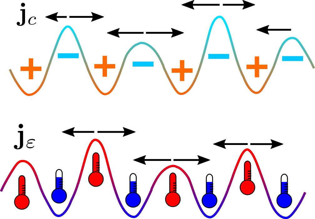
Figure 1: Charge (upper row) and energy currents (lower row) excited by wavelike longitudinal electric fields and temperature differences.

II main results

In this paper, we focus on the non-local transport properties and collective excitations of graphene electrons at the charge neutrality point - prime example for a Dirac fluid. The quantum Boltzmann method developed in Ref. Fritz2008 is used. This method relies on the fact, that at low temperatures the graphene fine structure constant $\alpha$ is renormalized to small values. Thermally excited electrons and holes therefore appear as sharply-defined quasiparticles, whose transport properties can be studied by means of a kinetic equation. The solution of this equation is facilitated by the presence of so-called collinear modes, whose scattering rates are enhanced by a large factor of $\log\left(1/\alpha\right)$. Here, the velocities of the interacting particles are parallel to each other. Due to the linear graphene spectrum, all particles travel at the same speed, regardless of their momentum. Particles traveling in parallel have a particularly long time to interact with each other, hence the strong enhancement. Transport in the hydrodynamic regime, however, is dominated by processes, which have the smallest scattering rates (for details see Eq. (27) and below). Such “slow” processes are represented by collinear zero modes – functions that set the collinear part of the collision operator to zero Fritz2008 ; Kashuba2008 .

We solve the kinetic equation by reducing it to a matrix equation in the space of collinear zero modes $\chi_{\mathbf{k},\lambda}^{\left(m,s\right)}=\lambda^{m}e^{im\theta}\left\{1,\lambda,\lambda\beta v\hbar k\right\}$ (see Sec. III.2). Here, $\theta$ is the polar angle and $k$ the modulus of the momentum variable $\mathbf{k}$, $\lambda=\pm 1$ is the band index, $m$ labels the angular harmonics $\exp\left(im\theta\right)$, and $s\in\left\{1,2,3\right\}$ labels the three basis functions written in curly brackets. To an excellent approximation, it is sufficient to retain only the $s=1$ and $s=3$ modes. These modes describe charge ($c$) and energy ($\varepsilon$) excitations, respectively. A numerical evaluation of the collision integral’s matrix elements with respect to the modes $\chi_{\mathbf{k},\lambda}^{\left(m,s\right)}$ (see Fig. 2) shows, that the relaxation rates of these modes grow linearly with increasing $m$:

$$\tau_{\varepsilon/c,m}^{-1}\sim\left|m\right|,$$ (1)

for large $m$ (see sections III.2 and IV.2). This unusual behavior allows us to solve the (linearized) Boltzmann equation exactly in the limit of a small $\alpha$. The details of this solution are given in Sec. IV.3.

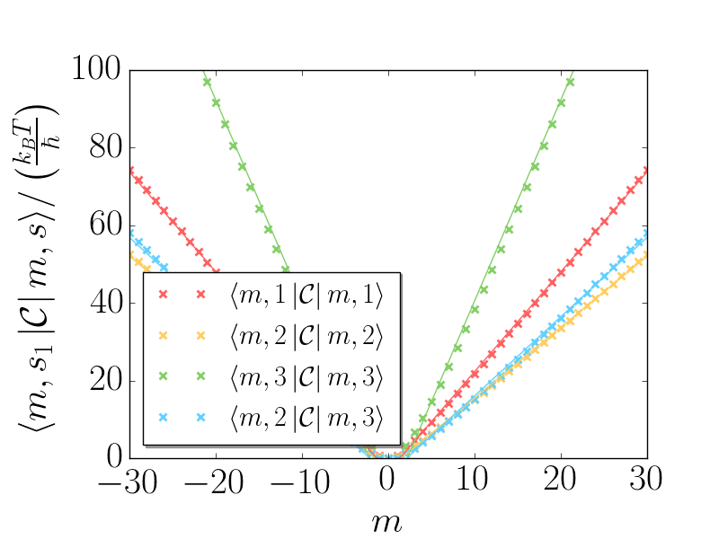
Figure 2: The matrix elements of the collision operator $\mathcal{C}$ of Eq. (III.1) with respect to the collinear zero modes $\chi_{\mathbf{k},\lambda}^{\left(m,s\right)}=\lambda^{m}e^{im\theta}\left\{1,\lambda,\lambda\beta v\hbar k\right\}$ of Eq. (32) grow linearly with increasing angular harmonic numbers $m$. The linear fits of Eqs. (51), (53) are plotted as solid red and green lines. The linear behavior of the matrix elements and scattering rates allows to solve the quantum Boltzmann equation exactly.

It is an important feature of graphene at the neutrality point, that the hydrodynamic modes excited by electric and thermal fields decouple in linear response, and in the absence of magnetic fields Mueller2008 ; Mueller2009 . The modes are characterized by the distinct scattering, with all of them following Eq. (1). Using our full solution of the Boltzmann equation, the non-local, i.e. wave-vector-dependent, charge and thermal conductivities as well as the non-local viscosity were calculated. The longitudinal and transverse non-local charge conductivities as functions of wave-vector $q$ and frequency $\omega$ are given by

$$\sigma_{\parallel} = \frac{\sigma_{0}}{1-i\tau_{c,1}\omega+\frac{1}{4}v^{2}\tau_{c,1}q^{2}\left(\frac{2i}{\omega}+\frac{1}{M_{c}\left(q,\omega\right)-i\omega}\right)},$$

$$\sigma_{\bot} = \frac{\sigma_{0}}{1-i\tau_{c,1}\omega+\frac{\frac{1}{4}v^{2}\tau_{c,1}q^{2}}{M_{c}\left(q,\omega\right)-i\omega}},$$ (2)

where $\sigma_{0}=\frac{2e^{2}\log\left(2\right)k_{B}T\tau_{c,1}}{\pi\hbar^{2}}$ is the conductivity at vanishing wave-numbers and frequencies Fritz2008 . $M_{c}$ is a memory function containing information on scattering in high angular momentum channels $m\geq 2$:

$$M_{c}\left(q,\omega\right)=\tau_{c,2}^{-1}+\frac{1}{2}vq\frac{\textrm{I}_{3+\frac{\eta_{c}}{\gamma_{c}}-i\omega\tau_{c}}\left(\tau_{c}vq\right)}{\textrm{I}_{2+\frac{\eta_{c}}{\gamma_{c}}-i\omega\tau_{c}}\left(\tau_{c}vq\right)}.$$ (3)

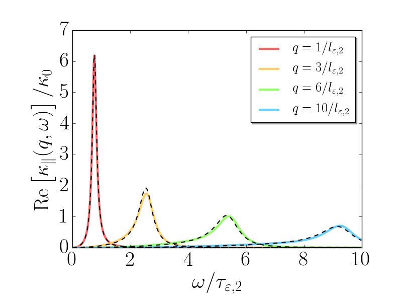
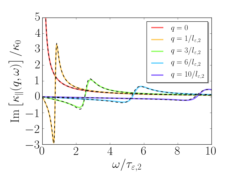
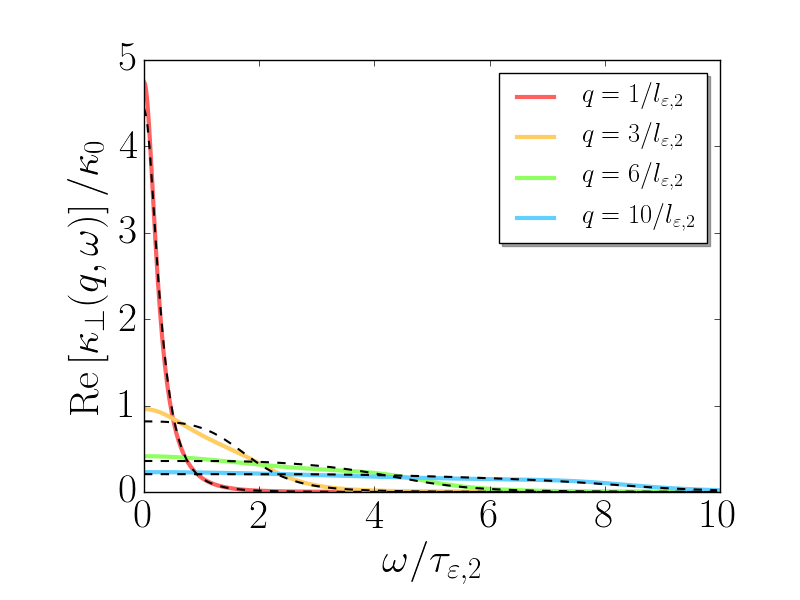
Figure 4: The figure shows the longitudinal (upper row) and transverse (lower row) thermal conductivities (64) as functions of the electric field frequency $\omega$. Different colors indicate different values of the wavenumber $q$. The conductivities are normalized to $\kappa_{0}=9N\pi^{3}k_{B}\zeta(3)\tau_{\varepsilon,2}/2\beta^{2}\hbar^{2}$. For small $\omega$ and vanishing $q$, the imaginary part of $\kappa_{\parallel/\perp}$ diverges as $1/\omega$, whereas the real part vanishes - a behavior indicating that thermal transport in the system is ballistic. The solid lines show the analytical result of Eq. (71), the dashed lines show the full numerical result including all modes and the exact scattering times.

This result is a direct consequence of the depence of the scattering rate $\tau_{c,m}^{-1}\sim\alpha^{2}k_{B}T\left|m\right|$ on the angular momentum state of the Dirac electron. A similar $\tau_{c,m}^{-1}\sim\left|m\right|$ behavior was found in Ref.Mirlin1997 for scattering off a random magnetic field and gives rise to similar expressions for the nonlocal conductivities, caused by rather different microscopic mechanism. In Eq. (3), $\tau_{c}$, $\gamma_{c}$ and $\eta_{c}$ determine the slopes and the offset in Eq. (1) (see Sec. IV.2). The results for the non-local thermal conductivity and viscosity are given in Eqs. (71), and (LABEL:eq:viscosity_result). The transport coefficients show pronounced resonance features at $vq\approx\omega$ where $q$ and $\omega$ are the wavenumber and frequency of the applied electric field or thermal gradient (see Figs. 3, 4) and $v$ is the electron group velocity. The longitudinal charge conductivity can be measured in experiments with surface acoustic waves (SAWs) Ingebrigtsen1969 ; Simon1996 ; Efros1990 ; Wixforth1989 ; Rotter1998 ; Govorov2000 . The transverse conductivity determines the skin effect, which is however not a feasible measurement for a two-dimensional graphene sheet. In section VI we consider a simple device consisting of a graphene sheet laid on top of a piezoelectric crystal. We calculate the velocity shift and damping of SAWs induced by the graphene sheet and find that, while damping effects are small, a substantial velocity shift can be expected. The damping and the velocity shift measured as functions of temperature can give important insights into the nature interaction effects in a Dirac fluid.

Non-local transport coefficients also determine in confined geometries. The latter case is illustrated in Sec. VII for the electric conductivity, using the Poiseuille geometry as an example. The constitutive relation linking the electric current to the electric field along the channel is interpreted as a differential equation (Eq. (93)) and solved with the appropriate boundary conditions (Eq. (94)). We find, that the flow profiles strongly depend on the channel width $w$ as compared to the electron-electron scattering lengths in the $m=1$ and $m=2$ channels: $l_{c,1}=v\tau_{c,1}$, $l_{c,2}=v\tau_{c,2}$. While $l_{c,1}$ governs the decay of charge currents, $l_{c,2}$ determines the effectiveness of current transfer from regions with high current density to regions with low current density. This latter mechanism is analogous to viscous momentum transfer. The flow profiles in dependence on $w$ can be separated into three regimes. For $w\gg l_{c,1}>l_{c,2}$, the samples are in the Ohmic regime, where the current is dissipated uniformly across the sample. The flow profile is flat. For $l_{c,1}<w<l_{c,2}$, the profile curvature is maximal, since on the one hand the current decay due to electron-electron scattering in the $m=1$ channel becomes inefficient, on the other hand the current transfer to the boundaries of the sample, where the flow is slowed down, is sufficiently strong. For even smaller widths $w<l_{c,2}$, the profile turns flat again, because the current transfer mechanism associated with $l_{c,2}$ ceases to be efficient. This characteristic pattern is shown in Fig. 12. Current profiles are accessible experimentally, e.g. through the scanning single electron transistor technique of Refs. Ella2019 ; Sulpizio2019 .

Finally, we calculated the dispersions of the collective modes of a Dirac fluid. As do the transport coefficients, the collective modes separate into a sector of charge excitations and a sector of energy and imbalance excitations ($s=2$). These two sectors are decoupled and can be studied separately. We find, that while the plasmon mode is gapped out at small wave-numbers due to the interaction induced resistivity (see Fig. 6), a so-called second sound mode, corresponding to a wavelike propagation of energy, appears (Fig. 9). Diffusive modes, corresponding to the diffusion of charge, heat and quasiparticles were found (see Figs. 5, 7). Their dispersion relations were calculated and showed to agree with known results Briskot2015 ; Torre2019 ; Phan2013 . Besides these well studied modes, an infinite set of damped modes connected to excitations in higher angular harmonic channels was found (see Figs. 5, 8). The dispersions of these modes are purely imaginary at vanishing wave-numbers and approach in the long wavelength limit the values $\omega_{m}\left(q=0\right)=-i/\tau_{\varepsilon/c,m}$ for the $m$-th angular harmonic in the energy ($\varepsilon$) or the charge ($c$) channels. At finite wave-numbers, these modes show a complex structure of merging branches. Similar modes play an important role in the equilibration of unitary fermi gases Brewer2015 and the QCD plasma Romatschke2016 ; Romatschke2018 ; Heller2018 . They also determine the unusual phase space dynamics of graphene electrons which was the subject of an earlier work Kiselev2019b .

Regime of validity

Transport in graphene is of interest to researchers with diverse backgrounds. Here we want to discuss the validity of our results in the context of other graphene related research. Our paper is concerned with the hydrodynmic regime, where electron tranport is governed by momentum conserving electron-electron collisions and the electron-electron mean free path is the smallest length scale Gurzhi1963 . In particular, momentum relaxing scattering off impurities and phonons must be weak. This demand sets serious limitations on sample sizes and on the temperature range.

II.0.1 The Dirac fluid of graphene at the charge neutrality point

Throughout the paper we are interested in the low energy effective behavior of graphene electrons near the Dirac point. Here, to a very good approximation, the electron dispersion is given by the massless two-dimensional Dirac Hamiltonian of Eq. (9) Castro2009 . At $T=0$, the lower Dirac cone is fully occupied and the upper Dirac cone is empty. At finite temperatures, electrons and holes in a region of size $k_{B}T$ around the Dirac cone are created. These quasiparticles are carriers of electric and thermal currents. Since their density is determined by temperature, $k_{B}T$ is the only energy scale in the system. We call this regime the Dirac fluid regime. The chemical potential is vanishingly small: $\mu\ll k_{B}T$. For the opposite case of a large chemical potential $\mu\gg k_{B}T$, the system enters the Fermi liquid regime. Here, the scattering rate is given by $\tau^{-1}\hbar\sim T^{2}/\mu$ Landau1957a ; Landau1957b ; Abrikosov1959 (up to logarithmic corrections in 2DHodges1971 ). For the quantum critical Dirac fluid, on the other hand, the electron-electron scattering rate is determined by the temperature alone:

$$\tau^{-1}\sim\alpha^{2}k_{B}T/\hbar$$ (4)

where $\alpha=e^{2}/\left(\varepsilon v\hbar\right)$ is the graphene fine structure constant. $v$ is the electron group velocity and $\varepsilon$ the dielectric constant. Higher order interaction effects can be treated in terms of the renormalization group. Integrating out high energy states above the thermal cut-off $k_{B}T$ results in a logarithmic increase of the electron’s group velocity Sheehy2007 ; Fritz2008 :

$$v=v_{0}\left(1+\frac{\alpha_{0}}{4}\log\left(\frac{\Lambda}{k_{B}T}\right)\right).$$ (5)

Here, $v_{0}\approx 10^{6}\,\mathrm{m}/\mathrm{s}$ and $\alpha_{0}$ are the unrenormalized, bare electron velocity and the fine structure constant. $\Lambda$ is an energy on the eV scale at which the electronic bands begin to deviate from the linear Dirac-like shape. It is essential to our theory, that the fine structure constant $\alpha\left(T\right)$ is renormalized to small values when the temperature is lowered. The system is gradually approaching the free Dirac fermion fixed point, thus ensuring the validity of the quasiparticle picture and the Boltzmann approach chosen here to study the transport of electrons. Eq. (5) is a perturbative result valid to lowest order in $\alpha$. However, experiments show that the logarithmic increase of the Fermi velocity at low energies is quite robust and holds even in the case of suspended graphene where $\alpha_{0}\approx 2$ as well as at intermediate temperatures Elias2011 . Thus, there is good reason to believe that even suspended graphene is located sufficiently near the free Dirac fermion fixed point, such that weak coupling results are physically meaningful; much more so for graphene grown on substrates with larger dielectric constants.

II.0.2 The quantum Boltzmann method

The quantum Boltzmann method is well established for systems with sharply defined quasiparticles KadanoffBaym ; Mahan , the prime example being the Fermi liquid Abrikosov1959 . Here, thermally excited quasiparticles have energies of the order of $\varepsilon_{\mathrm{qp}}=k_{B}T$, such that the ratio $\varepsilon_{\mathrm{qp}}/\left(\hbar\tau^{-1}\right)\sim\mu/k_{B}T\gg 1$ is large at temperatures below the Fermi temperature. This condition, which is based on phase-space arguments rather than the interaction strength, ensures the validity of the quasiparticle picture and the Boltzmann equation.

In the case of the Dirac fluid, the ratio of the characteristic qusiparticle energy and the scattering rate is

$$\frac{\varepsilon_{\mathrm{qp}}}{\tau^{-1}}\sim\alpha^{2}\left(T\right).$$ (6)

Thus, the quasiparticle picture is valid only at small coupling strengths. However, as discussed in the preceding section, for small temperatures $\alpha\left(T\right)$ decreases, and the Dirac fluid asymptotically approaches the free Dirac fermion limit. In this regime, the Boltzmann equation provides a powerfull tool for the study of transport phenomena. Coulomb interactions between electrons enter through a long-range Vlasov term which describes electrostatic forces due to an inhomogeneous charge distribution, as well as through the collision operator describing short-range electron-electron collisions. We use the collision operator derived in Ref. Fritz2008 , which includes all scattering processes to second order in the fine sctructure constant (Born approximation). While this approach is formally exact in the small $\alpha\left(T\right)$, low temperature limit, we believe, as argued above, that it should also provide reasonable results for larger values of the fine structure constant.

In this paper, we consider the linear response of the Dirac fluid to electric fields and thermal gradients at finite frequencies. The Boltzmann approach limits our discussion to small frequencies:

$$\omega\ll\frac{k_{B}T}{\hbar}.$$ (7)

At small frequencies, the system’s response is governed by intra-band processes which take place within one of the two Dirac cones. Inter-band processes, on the other hand, involve the creation of electron-hole pairs and therefore can only be excited at energies comparable to $k_{B}T$ Link2016 . This means that the off-diagonal elements of the density matrix $\left\langle\psi_{\lambda,\mathbf{k}}^{\dagger}\psi_{\lambda^{\prime},\mathbf{k}}\right\rangle,$where $\psi_{\lambda,\mathbf{k}}^{\dagger}$, $\psi_{\lambda,\mathbf{k}}$ are electron creation and anihilation operators and the band index $\lambda$ labes the two Dirac cones, are strongly suppressed. Allowing us to interpret the diagonal components as a distribution function

$$f_{\mathbf{k}\lambda}=\left\langle\psi_{\lambda,\mathbf{k}}^{\dagger}\psi_{\lambda,\mathbf{k}}\right\rangle$$

which can be found by solving the Boltzmann equation KadanoffBaym ; Mahan . For further details on the quantum Boltzmann approach we refer to Sec. III, Appendix A and Ref. Fritz2008 .

II.0.3 Impurities and Phonons

At the temperature of $\sim 50\,\mathrm{K}$, and assuming $\varepsilon\approx 5$, we estimate the electron-electron mean free path as $l_{ee}=v\tau\sim 2\,\upmu\mathrm{m}$. In clean graphene samples, impurity mean free paths of more than $10\upmu\mathrm{m}$ can be achieved Wang2013 , such that tranport indeed will be dominated by electron-electron scattering. A major concern in experiments with graphene near the charge neutrality point are small variations of the local chemical potential $\mu\left(\mathbf{x}\right)$ which have been dubbed electron-hole puddles Hwang2007 ; Martin2008 . While the origins and properties of electron puddles and their influence on transport are the subject of many studies (see e.g. Cheianov2007 ; Lucas2016 ; Gibertini2012 ; Sule2014 ), we choose not to include them in the present theory, which is concerned with interaction effects in a clean Dirac fluid. Our results are relevant for experiments with graphene sheets in the hydrodynamic regime. Here, the dominance of electron-electron scattering over any impurity induced effects was clearly demonstrated in Ref. Gallagher2019 by showing that the electron scattering rates grow linearly in accordance with Eq. (4) above a trashhold temperature.

Electron-phonon scattering is a significant disturbance for hydrodynamic electron flows at high temperatures, unless one is in a regime governed by phonon drag, see e.g. levchenko2020 . In graphene, the scattering of electrons by 2D graphene lattice phonons is limited by the small size of the Fermi-surface Efetov2010 , as well as by the high Debye temperature which loweres the phonon density of states Efetov2010 . These limitations are even more pronounced at the Dirac point, where due to momentum conservation only phonons with momenta $k_{\mathrm{ph}}<k_{B}T/v$ participate in scattering events. However, scattering with surface optical phonons of the substrate can lead to a significant increase of the sheet resistance at higher temperatures. In Ref. Chen2008 this mechanism was reported to set in above $150\,\mathrm{K}$ for graphene grown on SiO₂. To a large extend, scattering on surface acoustic photons determines the decay rates of graphene plasmons at finite charge densities Hwang2010 ; karimi2017 . Experiments on the hydrodynamics of Dirac fluids have been carried out with graphene sheets encapsuled in hexagonal boron nitride Crossno2016 ; Gallagher2019 . Here electron-phonon scattering is also reported to set in at the relatively high temperatures of $70\,\mathrm{K}$ Crossno2016 , or even to be insignificant up to room temperatures Gallagher2019 .

II.0.4 Sample sizes

Currently, high quality graphene sheets have sizes on the order of tenth of micrometers. On the one hand side this means that the effects of boundary scattering can be important Kiselev2019a . On the other hand, it has been demonstrated that such samples are sufficiently large to go well beyond the ballistic regime and to observe hydrodynamic behavior Sulpizio2019 ; KrishnaKumar2017 ; Crossno2016 ; Gallagher2019 ; Bandurin2016 ; Bandurin2018 ; Berdyugin2019 .

In graphene nanoribbons, gaps opening at the Dirac point can significantly influence the behavior of collective modes Son2006 ; karimi2017 . These gaps can be estimated as $\Delta\approx t/N$, where $t$ is a characteristic tight-binding hopping amplitude on the $1$eV scale and $N$ is the number of unit cells over which the ribbon extends. For hydrodynamic samples $N\approx 10^{5}$, and therefore the gaps are much smaller than quasiparticle energies at experimental temperatures.

Boundary effects on collective mode propagation will give a larger correction of order $l_{ee}/w$, where $w$ is the sample size (see e.g. wild2012 ).

III Theoretical framework

III.1 Kinetic equation

In order to clarify our notation, in this section we sketch the derivation of the quantum Boltzmann formalism for the Dirac fluid, which was developed in Ref. Fritz2008 . We begin with the Hamiltonian of graphene electrons at the charge neutrality point:

$$H=H_{0}+H_{\mathrm{int}},$$ (8)

where the free part is given by

$$H_{0}=v\hbar\int_{\mathbf{k}}\sum_{a,b,i}\psi_{a,i}^{\dagger}\left(\mathbf{k}\right)\left(\mathbf{k\cdot\sigma}\right)_{ab}\psi_{b,i}\left(\mathbf{k}\right),$$ (9)

and the interaction part reads

$$H_{\mathrm{int}}=\frac{1}{2}\int_{\mathbf{k},\mathbf{k}^{\prime},\mathbf{q}}\sum_{a,b,i,j}V\left(\mathbf{q}\right)\psi_{\mathbf{k+q},a,i}^{\dagger}\psi_{\mathbf{k}^{\prime}-\mathbf{q},b,j}^{\dagger}\psi_{\mathbf{k}^{\prime},b,j}\psi_{\mathbf{k,}a,i}.$$ (10)

$V\left(\mathbf{q}\right)=\frac{2\pi e^{2}}{\varepsilon\left|\mathbf{q}\right|}$ is the 2D Coulomb potential. The indices $i,j=1,2\,...,N=4$ refer to the spin and valley quantum numbers of an electron, whereas the two sub-lattices are labelled by the indices $a,b$. The free particle Hamiltonian $H_{0}$ is diagonalized by the unitary transformation

$$U_{\mathbf{k}}=\frac{1}{\sqrt{2}}\left[\begin{array}[]{cc}1&o_{\mathbf{k}}^{*}\\ 1&-o_{\mathbf{k}}^{*}\end{array}\right],$$ (11)

where $o_{\mathbf{k}}=\left(k_{x}+ik_{y}\right)/\sqrt{k_{x}^{2}+k_{y}^{2}}$.

For the derivation of the quantum Boltzmann equation, it is convenient to use the band representation of Dirac spinors $\psi_{\lambda,\mathbf{k}}=U_{\mathbf{k},\lambda a}\psi_{\mathbf{k},a}$ with $\lambda=\pm 1$ labeling the upper and lower Dirac cones. In this way, one can easily distinguish between processes that involve the creation of particle-hole pairs and those which do not. The thermally excited electron-hole pairs occupy states in a window of $k_{B}T$ around the Dirac point. Thus, if the applied fields have frequencies $\omega<2k_{B}T/\hbar$, which is true in the hydrodynamic regime, processes that create electron-hole pairs are unlikely and can be neglected. This translates to neglecting the off-diagonal components of the distribution function in the band representation, which is then given by its diagonal elements:

$$f_{\mathbf{k}\lambda}=\left\langle\psi_{\lambda,\mathbf{k}}^{\dagger}\psi_{\lambda,\mathbf{k}}\right\rangle.$$

The quantum Boltzmann equation then reads

$$\left(\partial_{t}+\mathbf{v}_{\mathbf{k}\lambda}\cdot\nabla_{\mathbf{r}}-\left(e\nabla\varphi_{\mathrm{tot}}\right)\cdot\nabla_{\mathbf{k}}+C\right)f_{\mathbf{k}\lambda}\left(\mathbf{r},t\right)=0.$$ (12)

Here, $\mathbf{v}_{\mathbf{k}\lambda}=\partial\varepsilon_{\mathbf{k}\lambda}/\partial\mathbf{k}$ is the group velocity and

$$\mathbf{\varphi_{\mathrm{tot}}}\left(\mathbf{r},t\right)=\varphi_{\mathrm{ext}}\left(\mathbf{r},t\right)+\varphi_{\mathrm{ind}}\left(\mathbf{r},t\right)$$ (13)

is the sum of the external electrostatic potential and the induced potential which is the result of an inhomogeneous distribution of charges. The term associated with $\varphi_{\mathrm{tot}}$ was first introduced by VlasovVlasov1938 . It will be dealt with at the end of this section. $C$ represents the central part of the kinetic theory - the Boltzmann collision operator describingelectron-electron Coulomb scattering. Details on the derivation of $C$ are summarized in Appendix A, based on Refs. Fritz2008 ; Kiselev2019b .

Studying the linear response to $\mathbf{\varphi_{\mathrm{tot}}}$, we expand the distribution function around the local equilibrium distribution $f_{k\lambda}^{\left(0\right)}$

$$f_{\mathbf{k}\lambda}\left(\mathbf{r},t\right)=f_{k\lambda}^{\left(0\right)}+w_{k}\psi_{\mathbf{k}\lambda}\left(\mathbf{r},t\right).$$ (14)

where $f_{k,\lambda}^{0}$ is given by

$$f_{k\lambda}^{\left(0\right)}=\frac{1}{e^{\beta\left(\varepsilon_{\mathbf{k}\lambda}-\mathbf{u}\cdot\mathbf{k}\right)}+1}.$$ (15)

The product $w_{k}\equiv f_{k}^{\left(0\right)}\left(1-f_{k}^{\left(0\right)}\right)$ , that will soon play the role of a weight function in the scalar product, does not depend on $\lambda$, and the corresponding index is dropped in Eq. (14) and in the following.

Performing a Fourier transformation $\psi{}_{\mathbf{k}\lambda}\left(\mathbf{r},t\right)\rightarrow\psi_{\mathbf{k}\lambda}\left(\mathbf{q},\omega\right)$ to frequency and momentum space, we obtain the linearized Boltzmann equation

$$\left({\cal L}+{\cal C}\right)\psi_{\mathbf{k}\lambda}\left(\mathbf{q},\omega\right)=S_{\mathbf{k}\lambda}\left(\mathbf{q},\omega\right).$$ (16)

$\mathcal{L}$ is the Liouville operator and given by

$${\cal L}=-i\omega+i\mathbf{q}\cdot\mathbf{v}_{\mathbf{k}\lambda}$$ (17)

The linearization of the collision operator can be expressed in the form

$${\cal C}\psi_{\mathbf{k}\lambda}\approx\frac{1}{w_{k}}\sum_{\lambda^{\prime}}\int_{\mathbf{k}^{\prime}}\frac{\delta\left(C\psi\right)_{\mathbf{k}\lambda}}{\delta\psi_{\mathbf{k}^{\prime}\lambda^{\prime}}}\psi_{\mathbf{k}^{\prime}\lambda^{\prime}},$$ (18)

where the weight function $w_{k}$ was introduced above.

Let the $\psi_{\boldsymbol{k}}$ be element of a function space with inner product

$$\left\langle\phi\mid\psi\right\rangle=\sum_{\lambda}\int_{\mathbf{k}}w_{k}\phi_{\mathbf{k}\lambda}^{*}\psi_{\mathbf{k}\lambda},$$ (19)

such that

$$\left\langle\phi\left|{\cal C}\right|\psi\right\rangle = \sum_{\lambda}\int_{\mathbf{k}}w_{k}\phi_{\mathbf{k}\lambda}^{*}{\cal C}\psi_{\mathbf{k}\lambda}$$ (20)

$$= \sum_{\lambda\lambda^{\prime}}\int_{\mathbf{k}\mathbf{k^{\prime}}}\phi_{\mathbf{k}\lambda}^{*}\frac{\delta\left(C\psi\right)_{\mathbf{k}\lambda}}{\delta\psi_{\mathbf{k}^{\prime}\lambda^{\prime}}}\psi_{\mathbf{k}^{\prime}\lambda^{\prime}}.$$

One can show that the entropy production in the absence of external driving terms is $\frac{\partial S}{\partial t}=k_{B}\left\langle\psi\left|{\cal C}\right|\psi\right\rangle$ which ensures that the collision operator is positive definite. In fact, ${\cal C}$ is Hermitian under the above scalar product. Therefore its eigenvalues are real and its eigenfunction form an orthonormal basis of the function space.

The right hand side of Eq. (16) is determined by the forces acting on the system. The three force terms studied here are due to electric fields, thermal gradients and viscous forces. For an electric field oriented along the $x$-axis, $\mathbf{E}=E_{0}\hat{\mathbf{e}}_{x}$, the force term reads

$$S_{E}=-eE_{0}\cos\theta\left(\lambda v\beta\right),$$ (21)

where $\theta$ is the polar angle of the momentum $\mathbf{k}$. It is important to notice, that

$$\mathbf{E}=-\nabla\varphi_{\mathrm{tot}}.$$

The corresponding term for a thermal gradient $\nabla T$ is given by

$$S_{T}=-k\left|\nabla T\right|\cos\theta k_{B}\left(v\beta\right)^{2}.$$ (22)

A viscous force is present if the drift velocity $\mathbf{u}$ in the local equilibrium distribution function (15) is a function of the coordinate $\mathbf{x}$. Then the drift term of the Boltzmann equation (12) can be thought of as a force term

$$S_{S} =-vkX_{0,\alpha\beta}\left(\frac{k_{\alpha}k_{\beta}}{k^{2}}-\frac{1}{2}\delta_{\alpha\beta}\right)\lambda\beta$$

$$=-\frac{1}{2}kX_{0}\sin\left(2\theta\right)\left(\lambda v\beta\right),$$ (23)

where the stress tensor is given by

$$X_{0,\alpha\beta} =\frac{1}{2}\left(\frac{\partial u_{\alpha}}{\partial x_{\beta}}+\frac{\partial u_{\beta}}{\partial x_{\alpha}}-2\delta_{\alpha\beta}\nabla\cdot\mathbf{u}\right).$$

In the following, we consider a flow with $\mathbf{u}\left(y\right)=u\left(y\right)\hat{\mathbf{e}}_{x}$ and therefore only include the component $X_{0,xy}$, which is relevant for the calculation of the shear viscosity.

The collision operator is given by

$$\left(C\psi\right)_{\mathbf{k}\lambda} = \frac{2\pi}{\hbar}\int_{k^{\prime}q}\delta\left(k+k^{\prime}-\left|\mathbf{k}+\mathbf{q}\right|-\left|\mathbf{k}^{\prime}-\mathbf{q}\right|\right)$$

$$\times \left(1-f_{k}^{\left(0\right)}\right)\left(1-f_{k^{\prime}}^{\left(0\right)}\right)f_{\left|\mathbf{k}+\mathbf{q}\right|}^{\left(0\right)}f_{\left|\mathbf{k}^{\prime}-\mathbf{q}\right|}^{\left(0\right)}$$

$$\times \left\{\gamma_{\mathbf{k},\mathbf{k}^{\prime},\mathbf{q}}^{\left(1\right)}\left(\psi_{\mathbf{k}+\mathbf{q},\lambda}+\psi_{\mathbf{k}^{\prime}-\mathbf{q},\lambda}-\psi_{\mathbf{k}^{\prime},\lambda}-\psi_{\mathbf{k},\lambda}\right)\right.$$

$$+ \left.\gamma_{\mathbf{k},\mathbf{k}^{\prime},\mathbf{q}}^{\left(2\right)}\left(\psi_{\mathbf{k}+\mathbf{q},\lambda}-\psi_{-\mathbf{k}^{\prime}+\mathbf{q},\bar{\lambda}}+\psi_{-\mathbf{k}^{\prime},\bar{\lambda}}-\psi_{\mathbf{k},\lambda}\right)\right\}.$$

The matrix elements $\gamma_{\mathbf{k},\mathbf{k}^{\prime},\mathbf{q}}^{\left(1\right)}$, $\gamma_{\mathbf{k},\mathbf{k}^{\prime},\mathbf{q}}^{\left(2\right)}$ can be found in Appendix A.

Another important term in the kinetic equation describes the electrostatic forces that arise due to an inhomogeneous distribution of charges. These forces are mediated by a self consistent potential $\varphi_{\mathrm{ind}}$, first introduced by Vlasov Vlasov1938 . It reads

$$e\varphi_{\mathrm{ind}}\left(\mathbf{r},t\right)=\alpha vN\int d^{2}r^{\prime}\sum_{\lambda}\int\frac{d^{2}k}{\left(2\pi\right)^{2}}\,\frac{\delta f_{\mathbf{k}\lambda}\left(\mathbf{r}^{\prime},\omega\right)}{\left|\mathbf{r}-\mathbf{r}^{\prime}\right|},$$ (25)

where we have used the abbreviation $\delta f_{\mathbf{k}\lambda}\left(\mathbf{r},\omega\right)=w_{k}\psi_{\mathbf{k},\lambda}\left(\mathbf{r},\omega\right)$ and multiplied the potential by $e$ for notational convenience. A derivation of the term can be found in Ref. KadanoffBaym (Eqs. (7-3) and (9-16)). Applying a Fourier transform to Eq. (25) one finds

$$e\varphi_{\mathrm{ind}}\left(\mathbf{q},t\right) = \alpha vN\sum_{\lambda}\int\frac{d^{2}k}{\left(2\pi\right)^{2}}\,\frac{2\pi\delta f_{\mathbf{k}\lambda}\left(\mathbf{q},\omega\right)}{q}.$$

In Sec. V we will not be interested in the response to the total electric field $\mathbf{E}=-i\mathbf{q}\varphi_{\mathrm{tot}}$, but rather in solutions of the homogeneous Boltzmann equation

$$\left({\cal L}+\mathcal{V}+{\cal C}\right)\psi_{\mathbf{k}\lambda}\left(\mathbf{q},\omega\right)=0.$$

Here, the Vlasov term

$$\mathcal{V}\psi_{\mathbf{k}\lambda}=-i\mathbf{q}\cdot\mathbf{v}_{\mathbf{k}\lambda}e\varphi_{\mathrm{ind}}.$$ (26)

has to be included explicitely.

III.2 Collinear zero modes

In this section, we summarize how Eq. (16) is solved in the limit of a small fine structure constant. A standard way to deal with an integral equation like (16) is to expand the function $\psi_{\mathbf{k},\lambda}$ into a set of suitable basis functions. The choice of this basis is facilitated by the fact that for small values of the graphene fine structure constant $\alpha$, the collision operator (III.1) logarithmically diverges if the velocities of involved particles are parallel to each other. This is a consequence of the linear single particle spectrum, and the resulting momentum independent velocity of massless Dirac particles. Intuitively speaking, the scattering is enhanced, because particles traveling in the same direction interact with each other over a particularly long period of time. A more mathematical picture of this so-called collinear scattering anomaly is presented in Appendix (B). It is convenient to write the collision operator as a sum of the collinear part $\mathcal{C}_{c}$ and the non-collinear part $\mathcal{C}_{nc}$:

$$\mathcal{C}=\log{\left(1/\alpha\right)}\mathcal{C}_{c}+\mathcal{C}_{nc}.$$ (27)

The factor $\log{\left(1/\alpha\right)}$ is large at small $\alpha$. Both operators, $\mathcal{C}_{c}$ and $\mathcal{C}_{nc}$, are hermitian with respect to the scalar product of Eq.19. Let $\varphi_{\mathbf{k},\lambda}^{n}$ be the orthogonal eigenfunctions of $\mathcal{C}_{c}$ such that

$$\left(\mathcal{C}_{c}\varphi^{n}\right)_{\mathbf{k},\lambda}=b_{n}\varphi_{\mathbf{k},\lambda}^{n}.$$ (28)

$\psi_{\mathbf{k},\lambda}$ is expanded in terms of these functions:

$$\psi_{\mathbf{k},\lambda}=\sum_{n}\gamma_{n}\varphi_{\mathbf{k},\lambda}^{n}.$$ (29)

Suppose, some of the orthogonal basis functions $\varphi^{n}$, namely those with $n<n_{0}$, set the collinear part of the collision operator to zero, i.e.

$$\mathcal{C}_{c}\varphi^{n<n_{0}}=0.$$ (30)

Then, inserting the expansion (29) into Eq. (16) and projecting it onto the basis functions $\varphi^{n^{\prime}}$, one finds

$$\gamma_{n^{\prime}>n_{0}}=\frac{\Braket{\varphi^{n^{\prime}}}{S}-\Braket{\varphi^{n^{\prime}}}{\left(\mathcal{L}+\mathcal{C}_{nc}\right)\psi}}{b_{n^{\prime}}\log{\left(1/\alpha\right)}}.$$ (31)

Hence, zero modes of $\mathcal{C}_{c}$ are enhanced by factor $\log{\left(1/\alpha\right)}$Fritz2008 . These colinear zero modes can be found from the collision operator given in Eq.III.1:

$$\chi_{\mathbf{k},\lambda}^{\left(m,s\right)}=\lambda^{m}e^{im\theta}\left\{1,\lambda,\lambda\beta v\hbar k\right\}.$$ (32)

Here, $m$ labels the angular momentum, $s\in\left\{1,2,3\right\}$ the modes $\left\{1,\lambda,\lambda\beta vk\right\}$, and $\theta$ is the polar angle of the momentum vector $\mathbf{k}$. All modes set the integral (III.1) to zero for collinear processes (see Appendix B).

From Eq. (31) follows that for small values of $\alpha$, only the collinear zero modes have to be retained in the expansion of the entire collision operator Eq. (29), i.e. the kinetic equation (12) can be solved using the restricted subspace of basis functions of Eq. (32). The stronger colinear scattering processes give rise to a rapid equilibration to the subset of modes given in Eq. (32) which then dominate the long-time dynamics.

In order to proceed, the matrix elements of Eq. (16) in this basis must be calculated. The matrix elements of the Liouville operator $\mathcal{L}$ are given by

$$\left\langle\chi_{\mathbf{k},\lambda}^{\left(m,s\right)}\left|\mathcal{L}\right|\chi_{\mathbf{k},\lambda}^{\left(m^{\prime},s^{\prime}\right)}\right\rangle=\left(-i\omega\delta_{m,m^{\prime}}+\frac{1}{2}ivq\left(e^{-i\vartheta_{\mathbf{q}}}\delta_{m,m^{\prime}+1}+e^{i\vartheta_{\mathbf{q}}}\delta_{m,m^{\prime}-1}\right)\right)\left(v\beta\hbar\right)^{-2}L_{s,s^{\prime}},$$ (33)

where $\vartheta_{\mathbf{q}}$ is the polar angle of the wave-vector $\mathbf{q}$ and

$$L=\left[\begin{array}[]{ccc}\frac{\log(2)}{\pi}&0&0\\ 0&\frac{\log(2)}{\pi}&\frac{\pi}{6}\\ 0&\frac{\pi}{6}&\frac{9\zeta(3)}{2\pi}\end{array}\right].$$ (34)

The rows and columns of the matrix notation refer to the mode index $s$ of Eq. (32).

We calculate the matrix elements of the collision operator $\mathcal{C}$ numerically (some values are given in Appendix C). Due to the rotational invariance of the low-energy Dirac Hamiltonian (8), they are diagonal in the angular harmonic representation. Most importantly, the matrix elements rapidly approach a linear behavior for large $\left|m\right|$:

$$\left\langle\chi_{\mathbf{k},\lambda}^{\left(m,s\right)}\left|\mathcal{C}\right|\chi_{\mathbf{k},\lambda}^{\left(m^{\prime},s^{\prime}\right)}\right\rangle=\frac{\delta_{m,m^{\prime}}}{v^{2}\beta^{3}\hbar^{3}}\left(\left|m\right|\gamma_{s,s^{\prime}}-\eta_{s,s^{\prime}}\right).$$ (35)

$\gamma_{s,s^{\prime}}$ and $\eta_{s,s^{\prime}}$ are numerical coefficients that are listed below Eqs. (51) and (53). This surprising result is due to the linear Dirac spectrum of the system. It allows to solve the Boltzmann equation exactly, as will be seen later. The linear behavior of the scattering rates is also shown in Fig. 2. To find closed expressions for the non-local transport coefficients, the scattering rates are approximated by Eq. (35) for $m>2$. In principle, the numerically exact scattering rates up to an arbitrary $m$ can be included. Here, the rates for $m>2$ will be assumed to follow Eq.35 in order to keep the algebraic efforts at a minimum. The projections of the force terms (21)-(23) onto collinear zero modes read

$$\Braket{S_{E}}{\chi_{\mathbf{k},\lambda}}=-\frac{eE_{0}}{2\hbar^{2}\beta v}\delta_{\left|m\right|,1}\left[\begin{array}[]{c}\frac{\log(2)}{\pi}\\ 0\\ 0\end{array}\right],$$ (36)

$$\Braket{S_{T}}{\chi_{\mathbf{k},\lambda}}=\frac{\left|\nabla T\right|k_{B}\pi^{4}}{v\beta\hbar^{2}}\delta_{\left|m\right|,1}\left[\begin{array}[]{c}0\\ \frac{\pi}{6}\\ \frac{9\zeta(3)}{2\pi}\end{array}\right],$$ (37)

$$\Braket{S_{S}}{\chi_{\mathbf{k},\lambda}} =-\frac{iX_{0}}{4\left(v\beta\hbar\right)^{2}}\textrm{sign}\left(m\right)\delta_{\left|m\right|,2}\left[\begin{array}[]{c}0\\ \frac{\pi}{6}\\ \frac{9\zeta\left(3\right)}{2\pi}\end{array}\right].$$ (41)

For the Vlasov term (26) one finds

$$\left\langle\psi_{\mathbf{k},\lambda}^{\left(m,s\right)}|\mathcal{V}|\psi_{\mathbf{k},\lambda}^{\left(m^{\prime},s^{\prime}\right)}\right\rangle = i\alpha N\left(e^{-i\vartheta_{\bm{q}}}\delta_{m,1}+e^{i\vartheta_{\bm{q}}}\delta_{m,-1}\right)$$ (45)

$$\times\frac{\delta_{1,s}\delta_{1,s^{\prime}}\delta_{m^{\prime},0}}{2v^{2}\beta^{3}\hbar^{3}}\left[\begin{array}[]{c}\frac{\log(2)^{2}}{\pi^{2}}\\ 0\\ 0\end{array}\right].$$

The non-equilibrium part of the distribution function expanded in the subset of colinear zero modes becomes

$$\psi_{\mathbf{k},\lambda}=\sum_{m=-\infty}^{\infty}\sum_{s=1}^{3}a_{m,s}\left(\omega,\mathbf{q}\right)\chi_{\mathbf{k},\lambda}^{\left(m,s\right)}.$$ (46)

Together, the expressions (16), (33), (35), (36)-(41), (45) and (46) provide a linearized kinetic equation restricted to the basis of collinear zero modes that becomes exact for small values of the fine structure constant $\alpha$. Since no assumptions on the spatial dependencies were made, except that they are be within the limits of the applicability of the kinetic equation, this expansion can be used to derive the non-local transport coefficients in the linear-response regime, as well as the dispersion relations of collective excitations.

IV Non-local Transport

IV.1 Effects of electron-hole symmetry, momentum conservation and thermal transport

Within the kinetic approach, the charge current $\mathbf{j}_{c}$ and the heat current $\mathbf{j_{\varepsilon}}$ are given by

$$\mathbf{j}_{c} =e\sum_{\lambda}\int_{\mathbf{k}}\lambda v\frac{\mathbf{k}}{k}f_{\mathbf{k},\lambda},$$ (47)

$$\mathbf{j_{\varepsilon}} =\sum_{\lambda}\int_{\mathbf{k}}v^{2}\hbar\mathbf{k}f_{\mathbf{k},\lambda}.$$ (48)

In these expressions intra-band processes that create particle-hole pairs are neglected (see Appendix A). It follows from Eqs. (47) (48), that the even in $\lambda$ part of the distribution function $f_{\mathbf{k},\lambda}$ contains information about thermal transport, whereas the odd part governs the transport of charge. Since the electric field contribution to the kinetic equation (21) is odd in $\lambda$, and the thermal gradient leads to a term that is even in $\lambda$ (Eq. (22)), the phenomena of thermal and charge transport are decoupled to linear order in the external fields at the neutrality point. This can be traced back to particle-hole symmetry and is the ultimate reason why the Wiedemann-Franz law is dramatically violated in a Dirac fluidCrossno2016 . The distribution function shows a similar decoupling ocf charge and heat modes for higher $m$: The collinear modes of Eq. (32) are proportional to $\lambda^{m}$ for $s=1$ and to $\lambda^{m+1}$ for $s=2,3$. Consequently the kinetic equation in the subspace of collinear zero modes is block diagonal in the $s=1$ and $s=2,3$ modes, as can be seen from Eqs. (III.1), (33), (36)-(41). In the following this will further simplify the calculation of transport coefficients.

Another important consequence of the linear graphene spectrum is that the heat current $\mathbf{j}_{\varepsilon}$ is proportional to the momentum density $\mathbf{g}=\sum_{\lambda}\int_{k}\hbar\mathbf{k}f_{\mathbf{k},\lambda}$ and is therefore conserved. The charge current, unlike in Galilean invariant systems, is not conserved, and decays due to interactions, giving rise to a finite restistvity in the clean system.

IV.2 Scattering times

The matrix elements of the collision operator determine the scattering rates of the three collinear zero modes in different angular harmonic channels. In the absence of spatial inhomogeneities and external forces, the kinetic equation in the basis of collinear zero modes (32) reads

$$\sum_{s^{\prime}}\left(\partial_{t}\delta_{s,s^{\prime}}+\Gamma_{m}^{s,s^{\prime}}\right)a_{m,s^{\prime}}=0,$$ (49)

where the $a_{m,s}$ are the coefficients of the expansion (46). Posed as an initial value problem, this equation describes the exponential decay of collinear zero modes. This decay governs the behavior of the system at long time scales, because modes that do not set the collinear part of the collision integral to zero decay faster by a factor $\log\left(1/\alpha\right)$ (see Eq. (27)).

The scattering rates $\Gamma_{m}^{s,s^{\prime}}$ are given by

$$\Gamma_{m}^{s,s^{\prime}}=\left(v\beta\hbar\right)^{2}L_{s,s^{\prime}}^{-1}\left\langle\chi_{\mathbf{k},\lambda}^{\left(m,s\right)}\left|\mathcal{C}\right|\chi_{\mathbf{k},\lambda}^{\left(m^{\prime},s^{\prime}\right)}\right\rangle.$$ (50)

Because of the definition of the scalar product in Eq. (19), the matrix elements have dimension ${\rm length}$${}^{2}/{\rm time}$. Vanishing scattering rates indicate conservation laws, and the corresponding modes are zero modes of the full collision operator as well as its collinear part. These modes reflect the conservation of particle density, imbalance density, energy density and momentum density:

$$\begin{array}[]{ccc}\chi_{\mathbf{k},\lambda}^{\left(s=1,m=0\right)}=1,&&\chi_{\mathbf{k},\lambda}^{\left(s=2,m=0\right)}=\lambda,\end{array}$$

$$\chi_{\mathbf{k},\lambda}^{\left(s=3,m=0\right)}=\lambda\beta v\hbar k,\qquad\chi_{\mathbf{k},\lambda}^{\left(s=3,m=1\right)}=\lambda e^{i\theta}\beta v\hbar k.$$

The imbalance density is conserved only to order $\alpha^{2}$, as it decays due to higher order interaction processes. An important simplification stems from the fact that all scattering rates, for large $\left|m\right|$, share the asymptotic behavior $\Gamma_{m}\sim\left|m\right|$. This becomes a reasonable approximation for the scattering rates with $m\geq 2$. In the next section it is shown, how this behavior allows us to obtain closed form expressions for the non-local transport coefficients. As discussed in the previous section, the matrix of scattering rates $\Gamma_{m}^{s,s^{\prime}}$ is block diagonal in the modes describing charge ($s=1$) and thermal excitations ($s=2,3$), i.e. $\Gamma_{m}^{1,2}=\Gamma_{m}^{2,1}=\Gamma_{m}^{1,3}=\Gamma_{m}^{3,1}=0$. Therefore, the scattering times determining the non-local electric conductivity are given by $\tau_{c,m}=1/\Gamma_{m}^{1,1}$: $\tau_{c,0}\rightarrow\infty$, $\tau_{c,1}=\frac{1}{\alpha^{2}}\frac{\hbar}{k_{B}T}\frac{\log 2}{0.804\pi}$, $\tau_{c,2}=\frac{1}{\alpha^{2}}\frac{\hbar}{k_{B}T}\frac{\log 2}{2.617\pi}$ as well as

$$\tau_{c,m} \approx\frac{1}{\alpha^{2}}\frac{\hbar}{k_{B}T}\frac{\log 2}{\pi}\left(\gamma_{c}\cdot\left|m\right|-\eta_{c}\right)^{-1}\,{\rm if}\ m>2,$$ (51)

where $\gamma_{c}=2.57$ and $\eta_{c}=3.45$ (see Appendix C for more numerical values). It is also convenient to define an effective scattering time for the Vlasov term:

$$\tau_{V}=\frac{2\pi^{2}\beta\hbar}{\alpha N\log\left(2\right)}.$$ (52)

Notice, that $\tau_{V}/\tau_{c,m}\sim 1/\alpha$ is large for small $\alpha$.

In the thermal sector, there are two relevant modes. However, the $s=3$ mode is physically more important, because the vanishing of the corresponding scattering rates for the $m=0$ and $m=1$ channels indicate the conservation of energy and momentum. In the following, it is shown that the neglecting of the $s=2$ imbalance mode in the calculation of the thermal conductivity and viscosity, while significantly simplifying the analysis, does only result in a small numerical error. Therefore, for the purpose of calculating the transport coefficients, only the $s=3$ energy mode will be considered. The scattering times are then given by $\tau_{\varepsilon,m}=1/\Gamma_{m}^{3,3}$. Because of energy and momentum conservation, we have $\tau_{\varepsilon,m=0,1}\rightarrow\infty$, and for $m=2$, it is $\tau_{\varepsilon,2}=\frac{1}{\alpha^{2}}\frac{\hbar}{k_{B}T}\frac{9\zeta(3)}{3.341\cdot 2\pi}$. For $m>2$ the linear approximation can be used:

$$\tau_{\varepsilon,m}\approx\frac{1}{\alpha^{2}}\frac{\hbar}{k_{B}T}\frac{9\zeta(3)}{2\pi}\left(\gamma_{\varepsilon}\cdot\left|m\right|-\eta_{\varepsilon}\right)^{-1}\ m>2,$$ (53)

with $\gamma_{\varepsilon}=5.18$ and $\eta_{\varepsilon}=11.3$.

IV.3 Non-local transport coefficients

The linear, non-local response of a system to external forces $\mathcal{F}\left(\mathbf{r}\right)$ is characterized by constitutive relations of the form

$$\mathcal{J}\left(\mathbf{r},t\right)=\int d^{d}r^{\prime}dt^{\prime}\,\nu\left(\mathbf{r}-\mathbf{r}^{\prime},t-t^{\prime}\right)\mathcal{F}\left(\mathbf{r}^{\prime},t^{\prime}\right),$$ (54)

where $\mathcal{J}\left(\mathbf{r},t\right)$ is a current sourced by the field $\mathcal{F}\left(\mathbf{r}^{\prime},t^{\prime}\right)$ and $\nu\left(\mathbf{r}-\mathbf{r}^{\prime},t-t^{\prime}\right)$ is the corresponding transport coefficient. $\mathcal{F}$ can be a scalar potential, a vector field (an electric field or a thermal gradient), or a tensor. Eq. (54) takes a much simpler form in Fourier space:

$$\mathcal{J}\left(\mathbf{q},\omega\right)=\nu\left(\mathbf{q},\omega\right)\mathcal{F}\left(\mathbf{q},\omega\right).$$ (55)

If the system is confined to a geometry of a characteristic size $l_{\mathrm{geo}}$, the relevant wave vectors $\mathbf{q}$ in Eq. (55) will be of the order of $q_{\mathrm{geo}}\approx 2\pi/l_{\mathrm{geo}}$. On the other hand $\nu\left(\mathbf{q},\omega\right)$ varies on scales of the inverse mean free path $q_{mf}\approx 2\pi/l_{mf}$, where $l_{mf}=v\tau$ and $\tau$ is the relevant relaxation time. Thus if $l_{\mathrm{geo}}\gg l_{mf}$, we can approximate $\nu\left(\mathbf{q}_{\mathrm{geo}},\omega\right)\approx\nu\left(\mathbf{q}=0,\omega\right)$. We then have

$$\nu\left(\mathbf{r}-\mathbf{r}^{\prime},\omega\right)\approx\nu_{0}\left(\mathbf{q}=0,\omega\right)\delta\left(\mathbf{r}-\mathbf{r}^{\prime}\right)$$ (56)

and the constitutive relation (54) reduces to its local form $\mathcal{J}\left(\mathbf{r},\omega\right)=\nu_{0}\left(\omega\right)\mathcal{F}\left(\mathbf{r},\omega\right)$. The non-locality of Eq. (54) matters if $l_{\mathrm{geo}}\lesssim l_{mf}$. On scales comparable to the mean free path, transport is intrinsically non-local, because particles loose their memory of previous events through collisions with other particles or impurities - a mechanism that ceases to be efficient. A good example is the Poiseuille flow through narrow channels described in Sec. VII. We proceed with the calculation of the non-local, i.e. wavenumber dependent electric conductivity, thermal conductivity and viscosity using the kinetic equation (12) and the collinear zero mode expansion summarized in Sec. III.2.

IV.3.1 Electric conductivity

As mentioned in Sec. IV.2, only the first collinear mode $s=1$ is involved in the calculation of the electric conductivity. Inserting the expansion of the distribution function in terms of collinear zero modes (46) into the kinetic equation (16) using its matrix representation of Eqs. (33), (35), (36)-(41) and (45), the left hand side of (16) can be transformed into a recurrence relation for the coefficients $a_{1,m}$, where, for the rest of this section, the $s=1$ index is dropped. A similar analysis for electrons in a random magnetic field was performed in Ref.Mirlin1997 . For $m>2$, Eq. (51) can be used, and the recurrence relation reads

$$a_{m+1}=\frac{2ie^{-i\vartheta_{\mathbf{q}}}}{vq}\left(i\omega-\tau_{c,m}^{-1}\right)a_{m}-e^{-2i\vartheta_{\mathbf{q}}}a_{m-1}.$$ (57)

This recurrence relation has the form

$$a_{m+1}=\left(\alpha^{\prime}m+\beta^{\prime}\right)a_{m}-e^{i\delta}a_{m-1}$$ (58)

with $\alpha^{\prime}=-\frac{2ie^{-i\vartheta_{\mathbf{q}}}}{vq}\frac{k_{B}T}{\hbar}\frac{\pi}{\log 2}\gamma_{c}$, $\beta^{\prime}=\frac{2ie^{-i\vartheta_{\mathbf{q}}}}{vq}\left(i\omega-\eta_{c}\frac{k_{B}T}{\hbar}\frac{\pi}{\log 2}\right)$ and $\delta=-2\vartheta_{\mathbf{q}}$. It has two solutions that can be given in terms of modified Bessel functions. The physically interesting solution is

$$a_{m}=c\cdot e^{i\frac{\delta}{2}\left(m+\frac{\beta^{\prime}}{\alpha^{\prime}}\right)}\mathrm{I}_{m+\frac{\beta^{\prime}}{\alpha^{\prime}}}\left(-\frac{2e^{i\delta/2}}{\alpha^{\prime}}\right),$$ (59)

where $\mathrm{I}_{\nu}\left(z\right)$ is the modified Bessel function of the first kind. Another solution that diverges for $m\rightarrow\infty$ is given by

$$c_{m}=c\cdot e^{i\frac{\delta}{2}\left(m+\frac{\beta^{\prime}}{\alpha^{\prime}}\right)}\mathrm{K}_{m+\frac{\beta^{\prime}}{\alpha^{\prime}}}\left(\frac{2e^{i\delta/2}}{\alpha^{\prime}}\right).$$

$\mathrm{K}_{\nu}$ is the modified Bessel function of the second kind. Making use of the coefficients $a_{m}$ for $m>2$ as given by Eq. (59), the kinetic equation can be reduced to a $5\times 5$ component matrix equation:

$$\left[\begin{array}[]{ccccc}-i\omega+M_{c}\left(q,\omega\right)&\frac{1}{2}ivqe^{i\vartheta_{\mathbf{q}}}&0&0&0\\ \frac{1}{2}ivqe^{-i\vartheta_{\mathbf{q}}}&-i\omega+\tau_{c,1}^{-1}&\frac{1}{2}ivqe^{i\vartheta_{\mathbf{q}}}&0&0\\ 0&\frac{1}{2}ivqe^{-i\vartheta_{\mathbf{q}}}&-i\omega&\frac{1}{2}ivqe^{i\vartheta_{\mathbf{q}}}&0\\ 0&0&\frac{1}{2}ivqe^{-i\vartheta_{\mathbf{q}}}&-i\omega+\tau_{c,1}^{-1}&\frac{1}{2}ivqe^{i\vartheta_{\mathbf{q}}}\\ 0&0&0&\frac{1}{2}ivqe^{-i\vartheta_{\mathbf{q}}}&-i\omega+M_{c}\left(q,\omega\right)\end{array}\right]\left[\begin{array}[]{c}a_{-2}\\ a_{-1}\\ a_{0}\\ a_{1}\\ a_{2}\end{array}\right]=\left[\begin{array}[]{c}0\\ \frac{eE_{0}\beta v}{2}\\ 0\\ \frac{eE_{0}\beta v}{2}\\ 0\end{array}\right],$$ (60)

where $M_{c}\left(q,\omega\right)=\tau_{c,2}^{-1}+a_{3}\left(q,\omega\right)/a_{2}\left(q,\omega\right)$ is a memory function containing information on scattering channels with higher angular momentum numbers. Using the Eqs. (58) and (59), the memory function is written

$$M_{c}\left(q,\omega\right)=\tau_{c,2}^{-1}+\frac{1}{2}vq\frac{\textrm{I}_{3+\frac{\eta_{c}}{\gamma_{c}}-i\omega\tau_{c}}\left(\tau_{c}vq\right)}{\textrm{I}_{2+\frac{\eta_{c}}{\gamma_{c}}-i\omega\tau_{c}}\left(\tau_{c}vq\right)},$$ (61)

with the abbreviation $\tau_{c}=\frac{\hbar}{k_{B}T}\frac{\log 2}{\pi}\gamma_{c}^{-1}$. It is now straightforward to calculate the electric conductivity from the relation

$$j_{c,x}\left(\mathbf{q},\omega\right)=\sigma_{xx}\left(\mathbf{q},\omega\right)E_{x}\left(\mathbf{q},\omega\right).$$ (62)

The non-local conductivity can be decomposed into a longitudinal part $\sigma_{\parallel}\left(\omega,q\right)$ and a transverse part $\sigma_{\bot}\left(\omega,q\right)$, both depending on the modulus of $\mathbf{q}$. The longitudinal and transverse parts describe currents that flow in the direction of $\mathbf{q}$, or orthogonal to $\mathbf{q}$, respectively:

$$\sigma_{\alpha\beta}=\frac{q_{\alpha}q_{\beta}}{q^{2}}\sigma_{\parallel}\left(q,\omega\right)+\left(\delta_{\alpha\beta}-\frac{q_{\alpha}q_{\beta}}{q^{2}}\right)\sigma_{\bot}\left(q,\omega\right).$$ (63)

We assumed that the electric field is parallel to the $x$-axis. According to Eq. (63), $\sigma_{\parallel}\left(q,\omega\right)$ can be read off from the $x$-component of the current density $j_{c,x}$ by letting $\mathbf{q}$ be parallel to $\mathbf{e}_{x}$, and $\sigma_{\bot}\left(q,\omega\right)$ by considering the case $\mathbf{q}\parallel\mathbf{e}_{y}$. The conductivities are then given by

$$\sigma_{\parallel} = \frac{\sigma_{0}}{1-i\tau_{1,c}\omega+\frac{1}{4}v^{2}\tau_{c,1}q^{2}\left(\frac{2i}{\omega}+\frac{1}{M_{c}\left(q,\omega\right)-i\omega}\right)},$$

$$\sigma_{\bot} = \frac{\sigma_{0}}{1-i\tau_{c,1}\omega+\frac{\frac{1}{4}v^{2}\tau_{c,1}q^{2}}{M_{c}\left(q,\omega\right)-i\omega}},$$ (64)

where $\sigma_{0}=N\frac{e^{2}\log\left(2\right)\tau_{c,1}}{2\pi\beta\hbar^{2}}$ is the quantum critical conductivity calculated in Ref. Fritz2008 . Note that $\sigma_{\parallel}\left(q\neq 0,\omega=0\right)=0$ holds, which also follows from formula (66). If this was not the case, static currents with a finite wave-vector $\mathbf{q}$ would lead to an infinite accumulation of charge at certain points, which is forbidden by the conservation of charge. In Fig. 3 the charge conductivities are plotted as functions of $\omega$ for different values of $q$.

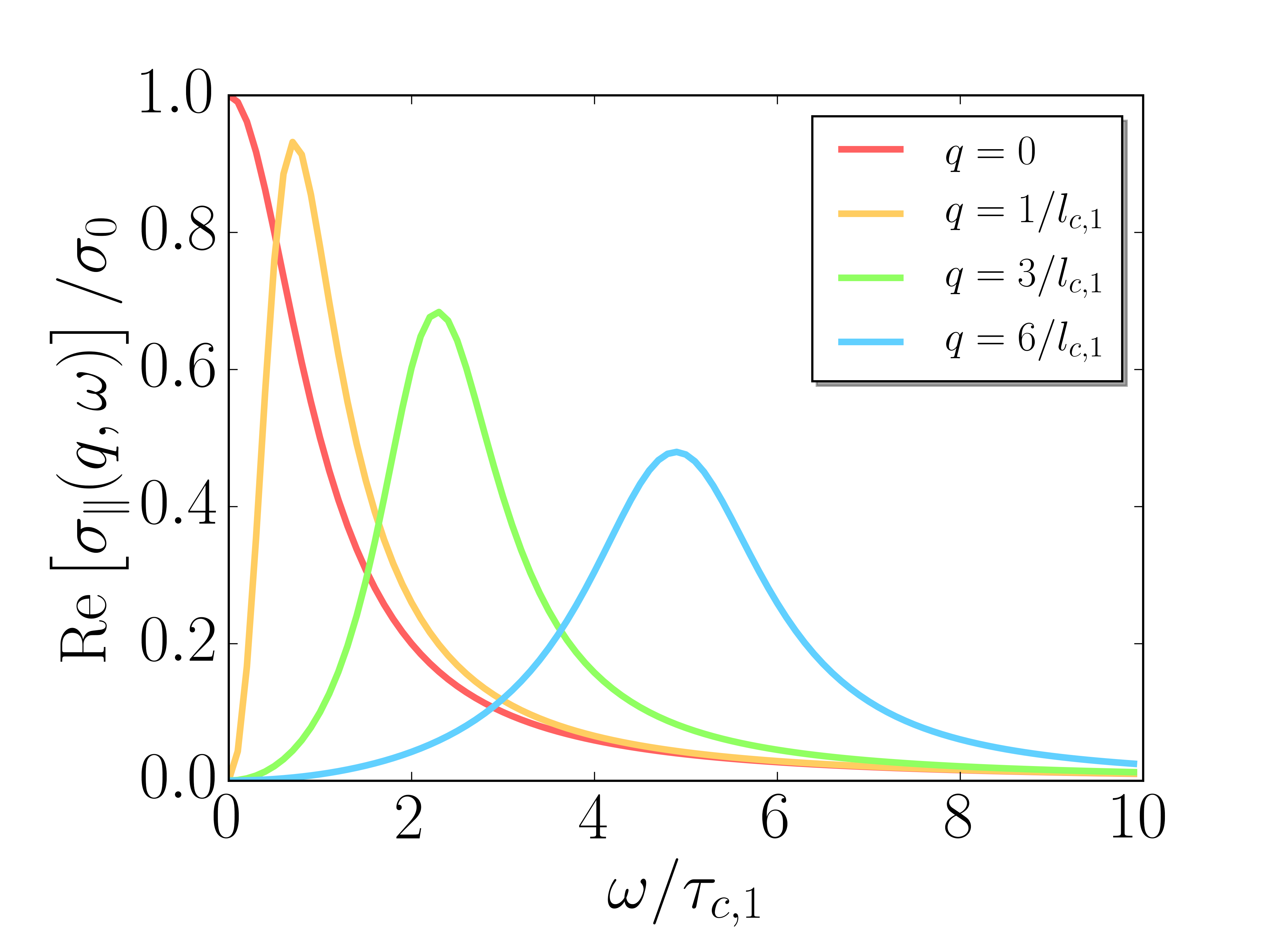
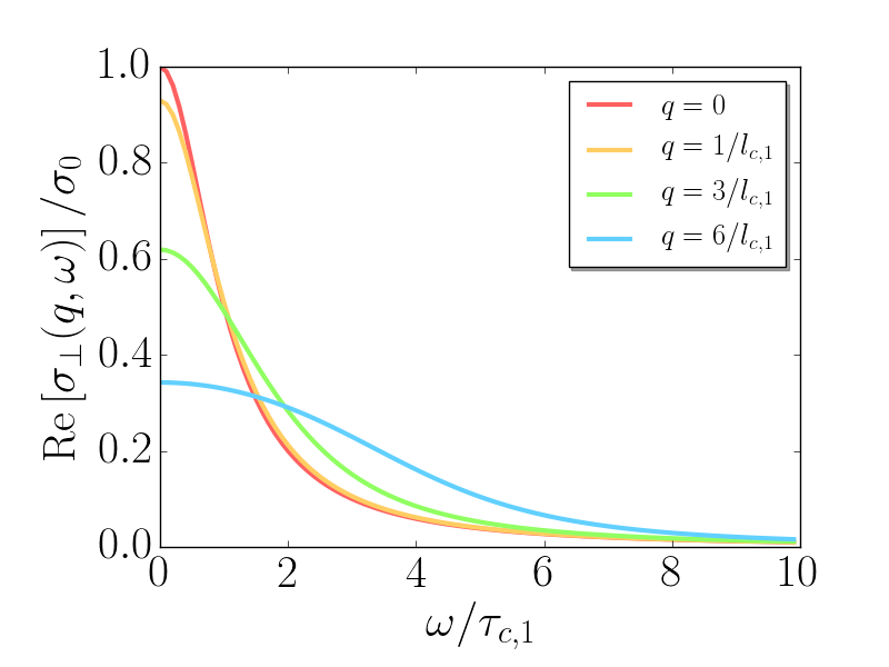
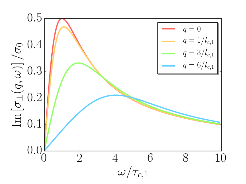
Figure 3: Longitudinal (upper row) and transverse (lower row) electric conductivities of charge neutral graphene as functions of the electric field frequency $\omega$ as given by Eqs (64). Different colors indicate different values of the wavenumber $q$. Frequencies and wave-numbers are normalized to the characteristic scattering times and lengths $\tau_{c,1}$, $l_{c,1}=v\tau_{c,1}$. $\sigma_{0}$ is the interaction induced conductivity at the neutrality point Fritz2008 ; Kashuba2008 . The graphs show distinct resonant features at frequencies $\omega\sim q/v$, where $v$ is the electron group velocity. Whereas the real part of the longitudinal and the imaginary part of the transverse conductivities are peaked around $\omega\sim q/v$, the imaginary part of the longitudinal conductivity exhibits a sign change indicating an abrubt phase change of the current response. The real parts approach $\sigma_{0}$ for $q\rightarrow 0$, $\omega\rightarrow 0$. For $q\neq 0$, $\omega=0$ the longitudinal conductivity vanishes. This general property of the charge conductivity follows from the conservation of charge (see Eq. (66)).

The electric conductivity tensor $\sigma_{\alpha\beta}\left(\mathbf{q},\omega\right)$ of Eq. (64) gives access to different electric response functions. The current-current correlation function is given by

$$\chi_{J_{\alpha}J_{\beta}}\left(\mathbf{q},\omega\right)=-i\omega\sigma_{\alpha\beta}\left(\mathbf{q},\omega\right)\,,$$ (65)

where $\alpha$, $\beta$ denote the components of the current vector (see e.g. Ref. Link2016 ). With the help of the continuity equation, the charge density-density correlation function is obtained from Eq. (65):

$$\chi_{\rho\rho}\left(q,\omega\right) =\frac{q_{\alpha}q_{\beta}}{\omega^{2}}\chi_{J_{\alpha}J_{\beta}}\left(\mathbf{q},\omega\right).$$

$$=\frac{q^{2}}{i\omega}\sigma_{\parallel}\left(q,\omega\right).$$ (66)

The non-local conductivity is related to the dielectric constant $\varepsilon\left(\mathbf{q},\omega\right)$ which is defined as (see Eq. (13))

$$\varepsilon=\frac{\varphi_{\mathrm{ext}}}{\varphi_{\mathrm{tot}}}.$$ (67)

Observing that $\varphi_{\mathrm{ind}}\left(\mathbf{q},\omega\right)=V\left(q\right)\delta\rho\left(\mathbf{q},\omega\right)$, where $\delta\rho$ is the induced charge density, we find

$$\varepsilon=1-V\left(q\right)\frac{\delta\rho}{\varphi_{\mathrm{tot}}}.$$ (68)

In linear response it is $\delta\rho=\chi_{\rho\rho}\left(q,\omega\right)\varphi_{\mathrm{tot}}$, so that we can write

$$\varepsilon=1-V\left(q\right)\chi_{\rho\rho}.$$ (69)

Taking the divergence of Ohm’s law $j_{\alpha}\left(\mathbf{q},\omega\right)=\sigma_{\alpha\beta}\left(\mathbf{q},\omega\right)E_{\beta}\left(\mathbf{q},\omega\right)$, and using the continuity equation $i\omega\delta\rho=iq_{\alpha}j_{\alpha}$ to express the electric current in terms of the induced charge density, we obtain

$$\varphi_{\mathrm{tot}}=\frac{i\omega\delta\rho}{q^{2}\sigma_{\parallel}}.$$

Inserting in Eq (68) we have

$$\varepsilon\left(\mathbf{q},\omega\right)=1-V\left(q\right)\frac{iq^{2}}{i\omega}\sigma_{\parallel}\left(\mathbf{q},\omega\right),$$

which is in accordance with Eq. (66). Notice, that both the longitudinal conductivity $\sigma_{\parallel}$ and the charge susceptibility $\chi_{\rho\rho}$ describe the response to the total potential $\varphi_{\mathrm{tot}}$. Hence the Vlasov term does not enter these quantities explicitely (for an in-depth discussion see Ref. PinesNozieres1 , Chapter 3, in particular Eq. (3.56)) Finally, the charge compressibility $K=\partial\rho/\partial\mu$ is given by

$$K\left(q\right)=\chi_{\rho\rho}\left(\omega=0\right).$$ (70)

The role of interaction effects for the compressibility were discussed in Ref.Sheehy2007 .

IV.3.2 Thermal conductivity

Next we presemt our analysis for the non-local thermal conductivity. Since momentum conservation implies for a Dirac fluid the conservation of the heat current, thermal transport is expected to display classical hydrodynamic behavior, i.e. one expects non-local effects to be even more important than for charge transport.Foster2009 ; Link2016 .

As pointed out in Sec. IV.2, the $s=3$ energy mode must be kept in the calculation of the thermal conductivity, whereas the $s=2$ imbalance mode can be neglected, contributing only a small correction to the overall result. With only a single mode involved, the calculation is formally analogous to the calculation of the electrical conductivity in Sec. IV.3.1, even though there are crucial differences in the actual result, given the distinct role of momentum conservation. The relaxation time $\tau_{c,m}$ must be replaced by $\tau_{\varepsilon,m}$ as given by Eq. (53). The conservation of momentum is incorporated via $\tau_{\varepsilon,1}\rightarrow\infty$, whivch follows from the Boltzmann approach. The resulting longitudinal and transverse thermal conductivities read

$$\kappa_{\parallel}\left(q,\omega\right) = \frac{\kappa_{0}}{i\omega\tau_{\varepsilon,2}-\frac{1}{4}v^{2}q^{2}\tau_{\varepsilon,2}\left(\frac{2i}{\omega}-\frac{1}{M_{\varepsilon}\left(q,\omega\right)+i\omega}\right)}$$

$$\kappa_{\bot}\left(q,\omega\right) = \frac{\kappa_{0}}{i\omega\tau_{\varepsilon,2}+\frac{\frac{1}{4}v^{2}q^{2}\tau_{\varepsilon,2}}{M_{\varepsilon,2}\left(q,\omega\right)+i\omega}},$$ (71)

with the memory function

$$M_{\varepsilon}\left(q,\omega\right)=\tau_{\varepsilon,2}^{-1}+\frac{1}{2}vq\frac{\textrm{I}_{3+\frac{\eta_{\varepsilon}}{\gamma_{\varepsilon}}+i\omega\tau_{\varepsilon}}\left(\tau_{\varepsilon}vq\right)}{\textrm{I}_{2+\frac{\eta_{\varepsilon}}{\gamma_{\varepsilon}}+i\omega\tau_{\varepsilon}}\left(\tau_{\varepsilon}vq\right)}.$$

The abbreviation $\tau_{\varepsilon,2}=\frac{1}{\alpha^{2}}\frac{\hbar}{k_{B}T}\frac{9\zeta(3)}{3.341\cdot 2\pi}$ is used. For convenience $\kappa_{\parallel/\bot}$ is given in units of a thermal conductivity $\kappa_{0}=9N\pi^{3}k_{B}\zeta(3)\tau_{\varepsilon,2}/2\beta^{2}\hbar^{2}$, however, $\tau_{\varepsilon,2}$ is the relaxation time in the $\left|m\right|=2$ channel, and should not be confused with an alleged relaxation time of the energy current, which is infinite due to the conservation of momentum.

In Fig. 3 the thermal conductivities are plotted as functions of $\omega$ for different values of $q$. The fact that thermal currents are protected by momentum conservation leads to a divergence of the thermal conductivity at small frequencies: for $q=0$, $\kappa$ is purely imaginary and shows the characteristic $1/\omega$ Drude behavior.

IV.3.3 Non-local shear viscosity

The non-local viscosity is defined through a constitutive relation of the form of Eq. (55), linking the shear force $X_{0,\alpha\beta}\left(\mathbf{r}^{\prime}\right)$ to the momentum-current tensor $\tau_{\alpha\beta}$:

$$\tau_{\alpha\beta}\left(\mathbf{r},t\right)=\int d^{2}r^{\prime}\int dt^{\prime}\,\eta_{\alpha\beta\gamma\delta}\left(\mathbf{r}-\mathbf{r}^{\prime},t-t^{\prime}\right)X_{0,\gamma\delta}\left(\mathbf{r}^{\prime},t^{\prime}\right).$$ (72)

Since the system is isotropic, the shear force can be chosen such that the flow velocity is aligned with the $x$-axis, and its gradient shows in the $y$ direction. It is assumed that the shear force is wavelike: $X_{0,xy}\left(\mathbf{r}\right)=X_{0,xy}e^{i\mathbf{q}\cdot\mathbf{r}-i\omega t}$. The wave-vector $\mathbf{q}$ can have an arbitrary direction in the $xy$-plane, introducing a preference direction to the system’s response. In addition to $\tau_{xy}$, this gives rise to nonzero components $\tau_{xx}$, $\tau_{yy}$, if $\mathbf{q}$ does not align with the $x$ or the $y$-axes. The viscosity tensor $\eta_{\alpha\beta xy}$ can be decomposed into transverse and longitudinal parts (see Eq. (63)) analogously to the electric and charge conductivities. Because $\eta_{\alpha\beta xy}$ is a fourth rank tensor the decomposition is slightly more involved and the reader is referred to Appendix D for details. The general $\mathbf{q}$-dependent viscosity tensor can be constructed with the help of three rank two tensors:

$$e_{\alpha\beta}^{\left(1\right)} = \frac{q_{\alpha}q_{\beta}}{q^{2}}$$

$$e_{\alpha\beta}^{\left(2\right)} = \delta_{\alpha\beta}-\frac{q_{\alpha}q_{\beta}}{q^{2}}$$

$$e_{\alpha\beta}^{\left(3\right)} = \frac{1}{\sqrt{2}}\left(q_{\alpha}p_{\beta}+p_{\alpha}q_{\beta}\right)/\left(pq\right),$$ (73)

where

$$p_{\alpha}=q_{\gamma}\varepsilon_{\gamma\alpha}.$$ (74)

The viscosity tensor is parameterized by two frequency and momentum dependent functions, $\eta_{\parallel}\left(\mathbf{q},\omega\right)$ and $\eta_{\bot}\left(\mathbf{q},\omega\right)$, which we will call longitudinal and transverse viscosities:

$$\eta_{\alpha\beta\gamma\delta}\left(\mathbf{q},\omega\right) =\eta_{1}\left(\mathbf{q},\omega\right)\left(e_{\alpha\beta}^{\left(1\right)}e_{\gamma\delta}^{\left(1\right)}+e_{\alpha\beta}^{\left(2\right)}e_{\gamma\delta}^{\left(2\right)}\right)$$

$$\qquad+\eta_{2}\left(\mathbf{q},\omega\right)e_{\alpha\beta}^{\left(3\right)}e_{\gamma\delta}^{\left(3\right)}.$$

Let the flow be in x-direction: $\mathbf{u}\left(y\right)=u\left(y\right)\mathbf{\hat{\mathbf{e}}}_{x}$, and let the wave-vector be parameterized by $\mathbf{q}=q\left(\cos\left(\vartheta_{\mathbf{q}}\right),\sin\left(\vartheta_{\mathbf{q}}\right)\right)^{T}$, where $\theta$ is measured with respect to the $x$-axis. For $\vartheta_{\mathbf{q}}=0$ or $\vartheta_{\mathbf{q}}=\pi/2$ follows $e_{\alpha\beta}^{\left(1,2\right)}=0$, $\eta_{xxxy}=\eta_{xxyx}=0$ and $\eta_{xyxy}=\eta_{2}/2$. This corresponds to the familiar shear flow in e.g. a Poiseuille geometry where $\tau_{xx}=\tau_{yy}=0$. The momentum current flows orthogonal to the direction of the momentum density. For $\vartheta_{\mathbf{q}}=\pi/4$, the viscosity is determined by $\eta_{1}$: $\eta_{xyxy}=\eta_{1}/2$.

As in the case of thermal conductivity, dropping the $s=2$ imbalance mode produces only a small numerical correction in the final result for the viscosity. With an external shear force of the form of Eqs. (23), (41) applied to the system, the kinetic equation can be written as $5\times 5$ component matrix equation, similar to the case of an applied electric field (see Eq. (60)). The force acts in the $\left|m\right|=2$ channels, and the equation reads

$$\left[\begin{array}[]{ccccc}-i\omega+M_{\varepsilon}\left(q,\omega\right)&\frac{1}{2}ivqe^{i\theta}&0&0&0\\ \frac{1}{2}ivqe^{-i\theta}&-i\omega&\frac{1}{2}ivqe^{i\theta}&0&0\\ 0&\frac{1}{2}ivqe^{-i\theta}&-i\omega&\frac{1}{2}ivqe^{i\theta}&0\\ 0&0&\frac{1}{2}ivqe^{-i\theta}&-i\omega&\frac{1}{2}ivqe^{i\theta}\\ 0&0&0&\frac{1}{2}ivqe^{-i\theta}&-i\omega+M_{\varepsilon}\left(q,\omega\right)\end{array}\right]\left[\begin{array}[]{c}a_{-2}\\ a_{-1}\\ a_{0}\\ a_{1}\\ a_{2}\end{array}\right]=\left[\begin{array}[]{c}-\frac{iX_{0}}{4}\\ 0\\ 0\\ 0\\ \frac{iX_{0}}{4}\end{array}\right].$$ (75)

Solving the matrix equation (75) for $a_{\pm 2}$, the viscosity is calculated with the help of Eq. (72) which takes the form $\tau_{xy}=N\sum_{\lambda}\int_{k}v_{x}k_{y}f_{\mathbf{k},\lambda}=\eta_{xyxy}X_{0,xy}$. As explained above, the viscosity components $\eta_{1}$ and $\eta_{2}$ can be read off from the general result $\eta_{xyxy}\left(\mathbf{q}=q\left(\cos\left(\vartheta_{\mathbf{q}}\right),\sin\left(\vartheta_{\mathbf{q}}\right)\right)^{T},\omega\right)$ by setting $\vartheta_{\mathbf{q}}=0$ and $\vartheta_{\mathbf{q}}=\pi/2$:

$$\eta_{1}\left(q,\omega\right) = \frac{2\eta_{0}}{-i\tau_{\varepsilon,2}\omega-q^{2}v^{2}\frac{i\tau_{\varepsilon,2}\omega}{2q^{2}v^{2}-4\omega^{2}}+\tau_{\varepsilon,2}M_{\varepsilon}\left(q,\omega\right)},$$

$$\eta_{2}\left(q,\omega\right) = \frac{2\eta_{0}}{-i\tau_{\varepsilon,2}\omega-\frac{q^{2}v^{2}\tau_{\varepsilon,2}}{4i\omega}+\tau_{\varepsilon,2}M_{\varepsilon}\left(q,\omega\right)}.$$

Here, $\eta_{0}$ is the viscosity at $q=0$, $\omega=0$, $\eta_{0}=N\left(k_{B}T\right)^{3}\tau_{\varepsilon,2}/\left(8\hbar^{2}v^{2}\right)$, as it was first calculated in Ref. Mueller2009 including both modes, $s=2$ and $s=3$.

V Collective modes

Collective modes are solutions to the homogeneous part of the kinetic equation (12), (16) (see e.g. Lucas2018 ). Consider Eq. (16). With the force terms set to zero it holds

$$\left(\mathcal{L}+\mathcal{V}+\mathcal{C}\right)\psi=0.$$

Here, $\mathcal{L}$ and $\mathcal{C}$ have are the matrix operators of Eqs. (33) and (35). Solutions to this equation exist only if

$$\det\left(\mathcal{L}+\mathcal{V}+\mathcal{C}\right)=0$$ (77)

holds. This is only the case for certain values of the variable pairs $\omega$, $q$. Eq. (77) is an eigenvalue problem where the eigenvalues $\omega\left(q\right)$ determine the dispersion relations of the collective modes. On the other hand, collective modes can be found from poles of response functions for an external force $S$. The two methods are equivalent. Within the kinetic equation formalism, response functions are calculated as averages over the distribution function $\psi=\left(\mathcal{L}+\mathcal{V}+\mathcal{C}\right)^{-1}S$. If the condition (77) is fulfilled, the operator $\left(\mathcal{L}+\mathcal{V}+\mathcal{C}\right)^{-1}$ is singular and thus singularities in the response to $S$ appear. We will use Eq. (77) to study the collective modes of a Dirac fluid on an infinite domain.

As in the previous sections, the kinetic equation will be expanded in terms of collinear zero modes (32): $\chi_{\mathbf{k},\lambda}^{\left(m,s\right)}=\lambda^{m}e^{im\theta}\left\{1,\lambda,\lambda\beta v\hbar k\right\}$. For $m=0$ these modes correspond to excitations of the charge, imbalance and energy densities; for $\left|m\right|=1$ they correspond to the associated currents. At the end of this section it will be shown that including non-collinear zero modes in the calculation does not change the result as long as the fine structure constant $\alpha$ is kept small.

To get a feeling for the structure of collective modes in the system, it is useful to begin with the case $q=0$. In the subspace of collinear zero modes, the kinetic equation reduces to Eq. (49) and the condition (77) reads

$$\det\left(-i\omega\delta_{s,s^{\prime}}+\Gamma_{m}^{s,s^{\prime}}\right)=0.$$ (78)

This is an eigenvalue equation for the frequencies of collective modes that can be solved independently for any $m$. Since, as pointed out in Sec. IV.1, $\Gamma_{m}^{s,s^{\prime}}$ is block-diagonal in the subspaces of electric ($s=1$) and imbalance/energy ($s=2,3$) excitations, the above equation, as well as its extension to $q\neq 0$, can be solved independently in these two sectors. For $s=1$, the eigenfrequencies are $\omega_{m}\left(q=0\right)=-i/\tau_{c,m}$. Since in this scenario the time evolution of the modes is given by the factor $e^{-i\omega_{m}t}$, all but the $m=0$ mode, which is protected by charge conservation, exponentially decay at a rate inversely proportional to their scattering time. The $m=0$ zero mode corresponds to the charge density, which is conserved, and therefore does not decay. In the following two sections, the collective charge, as well as energy and imbalance excitations will be described at finite $\mathbf{q}$. Figs. 5, 6, 7, 8, 9 show the dispersion relations of these modes.

V.1 Collective charge excitations

In general, conserved modes do not decay at $q=0$, and therefore their dispersion relations must vanish in a spatially homogeneous system. The only conserved mode in the charge sector is the charge density mode $\chi_{\mathbf{k},\lambda}^{\left(m=0,s=1\right)}=1$. In the limit $q\ll v\tau_{c,1}$, the memory matrix (61) reduces to $M_{c}\left(q,\omega\right)\approx\tau_{c,2}^{-1}$ and Eq. (77) can be solved analytically. The dispersions of the two lowest modes are

$$\omega_{\mathrm{charge\,diff.}}\approx\omega_{\pm}=-\frac{i}{2\tau_{c,1}}\pm\sqrt{\frac{vq}{\tau_{V}}-\frac{1}{4\tau_{c,1}^{2}}}.$$ (79)

The conserved charge density mode is described by $\omega_{-}$. The dispersion relations of Eq. (79) have a non-vanishing real part for

$$q>q_{pl}^{*}=\frac{\tau_{V}}{4v\tau_{c,1}^{2}}.$$ (80)

For wave-vectors below $q_{pl}^{*}$, the plasmon is over-damped (see Fig. 5). However, we have $vq_{pl}^{*}\sim\alpha^{3}k_{B}T/\hbar$ such that the plasmon mode becomes more and more pronounced at low temperatures.

The plasmon mode is gapped out due to the intrinsic interaction induced resistivity. At $q=0$ it has a vanishing real part and its decay rate is given by the scattering rate in the $m=1$ channel:

$$\omega_{pl}\left(q\rightarrow 0\right)=-i/\tau_{c,1}$$ (81)

(see also Briskot2015 ). It is the most weakly damped of an infinite set of modes corresponding to higher angular harmonics (see Fig. 5). It is clearly seen, that the modes relate to different angular harmonic channels $m$. For $q=0$ their dispersions approach $\omega_{m}\left(q=0\right)=-i/\tau_{c,m}$. Such modes play a crucial role in the relaxation mechanism of focused current beams in graphene Kiselev2019b . Similar collective modes have been argued to influence the relaxation behavior of unitary fermi gases Brewer2015 and QCD plasmas Romatschke2016 ; Romatschke2018 ; Heller2018 .

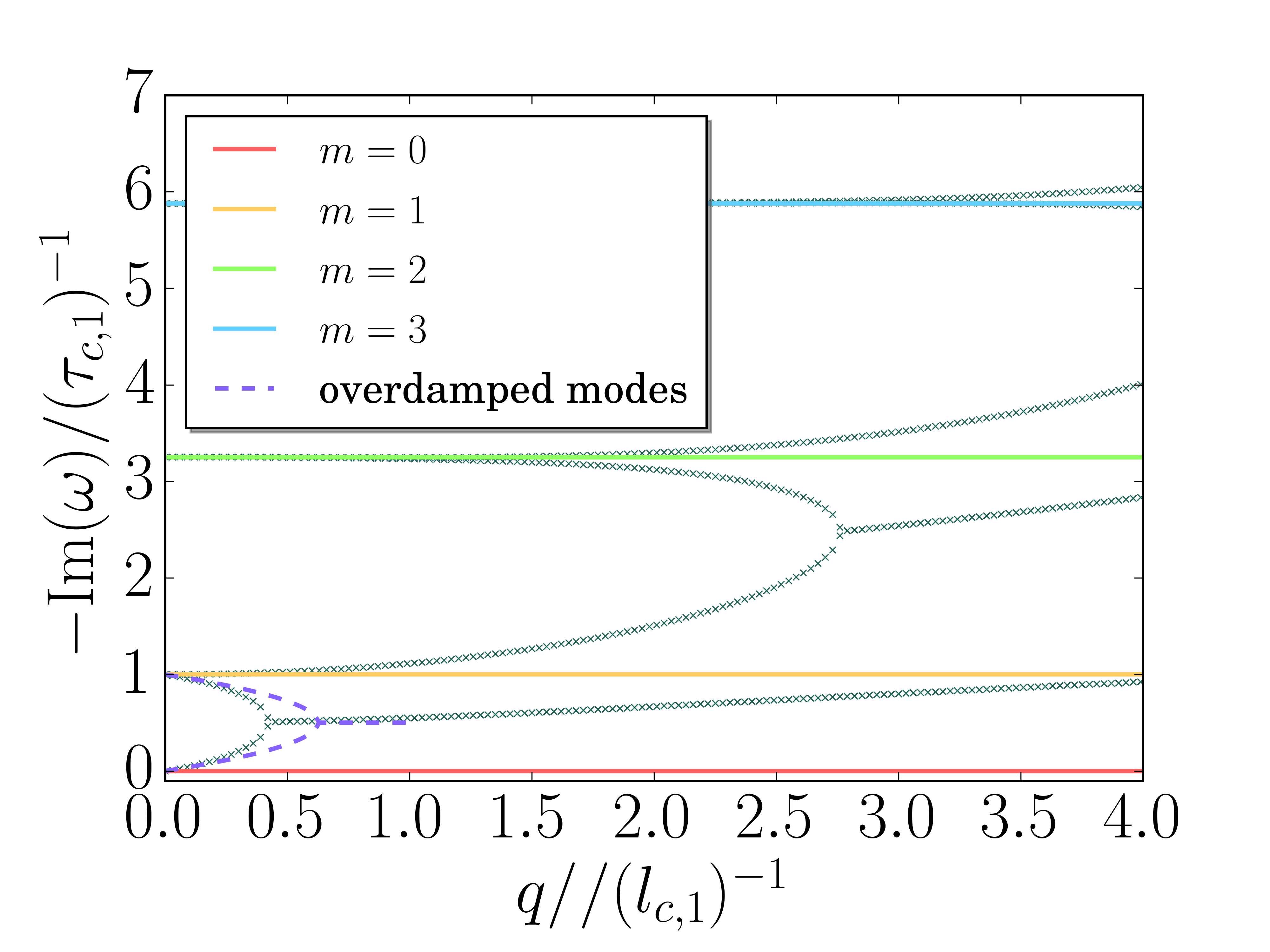
Figure 5: The imaginary parts of the dispersion relations of collective charge excitations in different angular harmonic channels $m$ are shown. The wave-vector $q$ is given in units of the inverse scattering length $v\tau_{c,1}^{-1}$. The grey symbols correspond to the numerical solution of Eq. (77). The purely imaginary $m=0$ diffusive mode is the only mode approaching zero for small $q$ - a behavior necessitated by charge conservation. Modes with a higher $m$ are damped and approach the values $-i/\tau_{c,m}$ for $q\rightarrow 0$. The corresponding excitations decay even in the absence of spatial inhomogeneities. At a value $q=q_{pl}^{*}$ (Eq. 80), the dispersions of the diffusive mode and the $m=1$ excitation merge, giving rise to a plasmon mode, which has a finite real part (see Fig 6). This value is slightly overestimated by the simplified expression of Eq. (80).

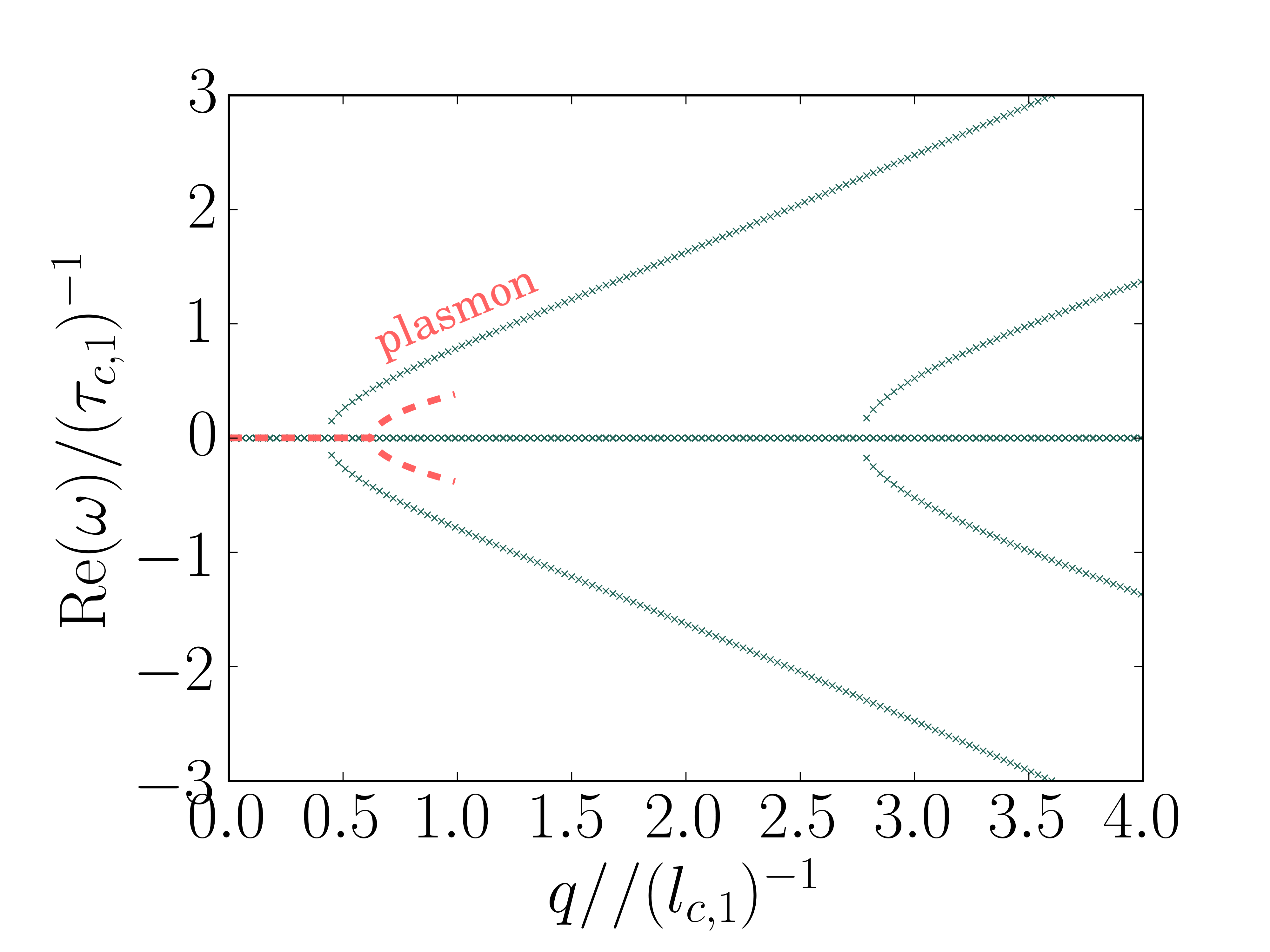
Figure 6: The figure shows the real parts of the dispersion relations of collective charge excitations in different angular harmonic channels $m$. The wave-vector $q$ is given in units of the inverse scattering length $v\tau_{c,1}^{-1}$. The grey symbols correspond to the numerical solution of Eq. (77). The plasmon mode is gapped out by the interaction induced conductivity and only obtains a finite real part around $q=q_{pl}^{*}$ (the simplified value of $q_{pl}^{*}$ given in Eq. (80) (red dashed line) overestimates the branching point). At higher $q$, other, strongly damped modes corresponding to higher angular harmonics appear. The dampings of these modes are given by the $m>1$ modes of Fig. 5.

V.2 Collective energy and imbalance excitations

In the energy sector spanned by the modes $s=2,3$, the Eqs. (77) and (78) give rise three zero eigenvalues. These correspond to the conserved energy ($\chi_{\mathbf{k},\lambda}^{\left(m=0,s=3\right)}=\lambda\beta v\hbar k$) and quasiparticle (imbalance) densities ($\chi_{\mathbf{k},\lambda}^{\left(m=0,s=2\right)}=\lambda$), as well as momentum ($\chi_{\mathbf{k},\lambda}^{\left(m=1,s=3\right)}+\left(-\right)\chi_{\mathbf{k},\lambda}^{\left(m=-1,s=3\right)}=2\left(i\right)\beta v\hbar k_{x\left(y\right)}$). The first two conservation laws lead to two diffusive modes. The conservation of momentum gives rise to second sound - ballistic thermal waves propagating through the two dimensional graphene plane Phan2013 . This mode is the analogue of the density modes of a clean neutral Galilean invariant system.

Truncating the mode expansion of Eq. (77) at $m=2$, which is a good approximation for low wave-numbers, yields the dispersions

$$\omega_{\mathrm{heat\,diff.}} \approx\frac{1}{4}v^{2}q^{2}\tau_{\varepsilon,2},$$

$$\omega_{\mathrm{qp\,diff.}} \approx\frac{1}{8}v^{2}q^{2}\tau_{\varepsilon,2},$$ (82)

for the heat and quasiparticle (imbalance) diffusion modes, respectively. The second sound dispersion is given by

$$\omega_{\mathrm{sec.\,sound}}\approx\frac{vq}{\sqrt{2}}+i\tau_{\varepsilon,2}\frac{v^{2}q^{2}}{8}.$$ (83)

Second sound mediated by phonons has been previously observed in solids Narayanamurti1972 and had a velocity comparable to the velocity of sound. Here, the second sound is carried by electrons and propagates with a velocity $v_{0}/\sqrt{2}$. The above dispersion relations are shown in Figs. 7 and 9.

Figure 7: The figure shows the imaginary part of the dispersion relations of second sound, heat diffusion, and quasiparticle (imbalance) diffusion excitations. The wavevector $q$ is given in units of the inverse scattering length $v\tau_{c,2}^{-1}$. The grey symbols correspond to the numerical solution of Eq. (77). The damping of second sound is due to scattering in the $m=2$ channel and follows the dispersion $\mathrm{Im}\left(\omega_{\mathrm{sec.\,sound}}\right)\approx\frac{1}{8}v^{2}q^{2}\tau_{\varepsilon,2}$ (red curve). For small $q$ the imaginary part of the second sound dispersion and the dispersion of the quasiparticle diffusion mode merge. A third diffusive mode corresponds to the diffusion of heat (orange curve).

The dispersion of the quasiparticle diffusion mode and the imaginary part of the second sound dispersion merge at low wave-numbers. As in the case of charge excitations, there exists an infinite number of damped modes associated with scattering in higher angular harmonic channels. These modes are depicted in Figs. 8 and 9. Note, that modes associated with imbalance excitations ($s=2$) are damped stronger by an order of magnitude as compared to energy excitations ($s=3$).

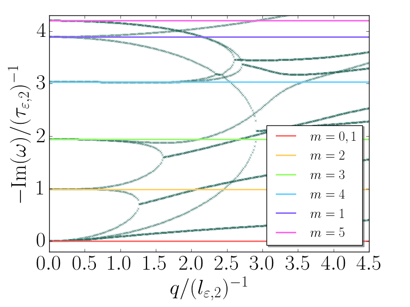
Figure 8: The imaginary part of the dispersion relations of collective charge excitations in different angular harmonic channels $m$ are shown. The wave-vector $q$ is given in units of the inverse scattering length $v\tau_{c,2}^{-1}$. The grey symbols correspond to the numerical solution of Eq. (77). For small $q$, the modes approach values given by the scattering rates $-i/\tau_{c,m}$ and are thus strongly damped. At larger values of $q$, the dispersions tend to merge in a complex fashion. Fig. 7 shows the weakly damped modes (second sound and diffusive modes) for small values of $q$.

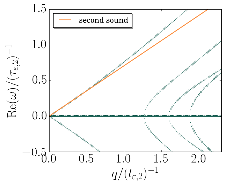
Figure 9: The real parts of the dispersion relations of collective energy and imbalance excitations are depicted. The grey symbols correspond to the numerical solution of Eq. (77). The linear dispersion of the second sound mode given by $vq/\sqrt{2}$ for small $q$ is shown in orange color. The wave-vector $q$ is given in units of the inverse scattering length $v\tau_{c,2}^{-1}$.

V.3 Validity of the collinear zero mode approximation for collective modes

The discussion so far was carried out in the restricted subspace of collinear zero modes. In this section it is shown that the results for collective excitations obtained within the restricted subspace remain valid, if this restriction is lifted, and non-collinear zero modes are added. These modes introduce large corrections to the matrix of scattering rates $\Gamma_{m}^{s,s^{\prime}}$, and it is not obvious that they can be neglected. It is sufficient to consider the $\mathbf{q}=0$ case. The extension to finite wave-numbers is straightforward.

The scattering rate matrix $\Gamma_{m}^{s,s^{\prime}}$ of Eq. (50) is extended to include modes that are not collinear zero modes, which are labeled with indices $s>3$. It is useful to define the following matrices

$$S =\left(v\beta\hbar\right)^{2}\left\langle\chi_{\mathbf{k},\lambda}^{\left(s<3\right)}\left|\mathcal{C}\right|\chi_{\mathbf{k},\lambda}^{\left(s^{\prime}<3\right)}\right\rangle$$

$$P =\left(v\beta\hbar\right)^{2}\left\langle\chi_{\mathbf{k},\lambda}^{\left(s>3\right)}\left|\mathcal{C}\right|\chi_{\mathbf{k},\lambda}^{\left(s^{\prime}<3\right)}\right\rangle$$

$$Q =\left(v\beta\hbar\right)^{2}\left\langle\chi_{\mathbf{k},\lambda}^{\left(s<3\right)}\left|\mathcal{C}\right|\chi_{\mathbf{k},\lambda}^{\left(s^{\prime}>3\right)}\right\rangle$$

$$R =\left(v\beta\hbar\right)^{2}\left\langle\chi_{\mathbf{k},\lambda}^{\left(s>3\right)}\left|\mathcal{C}\right|\chi_{\mathbf{k},\lambda}^{\left(s^{\prime}>3\right)}\right\rangle.$$

Here, $\chi_{\mathbf{k},\lambda}^{\left(s<3\right)}$ are the familiar collinear zero modes (32). $\chi_{\mathbf{k},\lambda}^{\left(s>3\right)}$ are modes with a different $\left|\mathbf{k}\right|$-dependence, such that the full set of modes forms a complete basis. Since $\mathcal{C}$ is Hermitian, we have $Q=P^{T}$. The mode expansion of the Liouville operator $L_{s,s^{\prime}}$ of Eq. (33) also has to be enlarged by the $s>3$ modes. However, we do not need to know the precise values of the corresponding elements of $L$. The eigenvalue equation (78) reads

$$\det\left(-i\omega L-F\right)=0,$$ (84)

where $F$ is the composite matrix

$$F=\left[\begin{array}[]{cc}S&P\\ P^{T}&R\end{array}\right].$$

In the following, the Liouville matrix $L$ will also be separated into blocks corresponding the same subspaces: $L=\left(\left(L_{S},L_{P}\right),\left(L_{P}^{T},L_{S}\right)\right)$. It follows from Eq. (27) and the Hermiticity of the collinear part of the collision operator $\mathcal{C}_{c}$ that

$$S \sim P\sim 1$$

$$R \sim\log\left(1/\alpha\right),$$

meaning that non collinear zero modes are scattered faster by a factor of $\log\left(1/\alpha\right)$. The determinant can be found using the block matrix identity

$$\det\left[\begin{array}[]{cc}A&B\\ C&D\end{array}\right]=\det\left(D\right)\det\left(A-BD^{-1}C\right).$$ (85)

Applying this identity to Eq. (84) and noticing that for $\alpha\rightarrow 0$ the inverse matrix in the last determinant vanishes, one has

$$\det\left(i\omega L+F\right)\approx\det\left(i\omega L_{R}+R\right)\det\left(i\omega L_{S}+S\right).$$

Eq. (84) therefore separates into two independent parts: $\det\left(i\omega L_{R}+R\right)=0$ and $\det\left(i\omega L_{S}+S\right)=0$. The second equation is equivalent to the eigenvalue equation (78). In the limit of a small fine structure constant, the weakly damped collective modes can therefore be found by solving the kinetic equation in the restricted subspace of collinear zero modes, even if there is significant coupling between all modes.

VI Surface acoustic waves

The longitudinal electrical conductivity $\sigma_{\parallel}$ is accessible through experiments with surface acoustic waves (SAWs) Wixforth1989 . The simplest setup to measure $\sigma_{\parallel}$ is a sheet of graphene placed on top of a piezoelectric material. Using interdigital transducers, SAWs are induced in the piezoelectric. The real part of $\sigma_{\parallel}$ then determines the damping of the SAWs, while the imaginary part changes the SAW velocity $v_{s}$. Overall, for a small piezoelectric coupling the change of the SAW velocity $\Delta v_{s}$, where the imaginary part describes the damping, can be written as Ingebrigtsen1969 ; Simon1996

$$\frac{\Delta v_{s}}{v_{s,0}}=p_{e}\frac{1}{1+i\frac{\sigma_{\parallel}}{\sigma_{M}}}.$$ (86)

Here $p_{e}<1$ is an effective coupling constant, and a $\sigma_{M}$ a reference conductivity. Both $p_{e}$ and $\sigma_{M}$ depend on material parameters of the piecoelectric. A rough estimate for $\sigma_{M}$ is given by $\sigma_{M}\approx v_{s}\epsilon_{\mathrm{eff}}$ Ingebrigtsen1969 ; Simon1996 , where $\epsilon_{\mathrm{eff}}$ is the effective permittivity at the surface of the piezoelectric. There has been experimental work on the coupling between SAWs and graphene Bandhu2013 ; Miseikis2012 . LiNbO₃ seems to be a suitable piezoelectric for such experimentsBandhu2013 , because it provides a relatively large coupling parameter $p_{e}\approx 0.03$ Rotter1998 . While there might be better choices for the piezoelectric material, here we consider LiNbO₃, since the feasibility of a graphene-LiNbO₃ device has been demonstrated in Ref. Bandhu2013 . The SAW velocity is $v_{s}\approx 4\cdot 10^{3}\,\mathrm{m/s}$ and the effective dielectric constant is given by $\epsilon_{\mathrm{eff}}\approx 0.5\epsilon_{0}\left(\sqrt{\epsilon_{xx}^{T}\epsilon_{zz}^{T}}+2\right)\approx 24\epsilon_{0}$ (assuming that the dielectric constant above the graphene sheet is $\epsilon_{0}$). One then has

$$\sigma_{M}\approx 10^{-6}\,\mathrm{S}.$$

The fine structure constant is small due to the large dielectric constant and renormalization effects. We estimate $\alpha\approx 0.1.$ Here and in the following estimations, we assume a temperature of $50\,\mathrm{K}$.

Interdigital transducers induce SAWs with sharply defined wave-vectors $q_{0}$. The frequency of the SAW $\omega_{0}$ is given by

$$\omega_{0}=v_{s}q_{0}.$$

$\omega_{0}$ is much smaller than the characteristic hydrodynamic frequency for a wave-vector of the same magnitude $\omega_{\mathrm{hydro}}\approx vq_{0}$, where $v\approx 10^{6}\,\mathrm{m}/\mathrm{s}$. It is

$$\frac{\omega_{0}}{\omega_{\mathrm{hydro}}}\approx 0.005.$$ (87)

As shown in Fig. 3 the longitudinal conductivity $\sigma_{\parallel}$ is peaked around $\omega_{\mathrm{hydro}}$ and vanishes in the limit $\omega=0$, $q\rightarrow 0$. Therefore, SAW experiments are confined to a highly “off-resonant” regime due to the small ratio (87) and therefore cannot be large.

The damping coefficient is given by

$$\Gamma=-\omega\mathrm{Im}\left(\frac{\Delta v_{s}}{v_{s}}\right)=\omega p_{e}\frac{\mathrm{\mathrm{Re}}\left(\sigma_{\parallel}\right)/\sigma_{M}}{1+\left|\frac{\sigma_{\parallel}}{\sigma_{M}}\right|^{2}}.$$ (88)

The relative velocity shift is

$$\mathrm{Re}\left(\frac{\Delta v_{s}}{v_{s}}\right)=p_{e}\frac{1+\mathrm{\mathrm{Im}}\left(\sigma_{\parallel}\right)/\sigma_{M}}{1+\left|\frac{\sigma_{\parallel}}{\sigma_{M}}\right|^{2}}.$$ (89)

Since interdigital transducers excite SAWs of a fixed wavelength, altering $q_{0}$ is difficult. Instead, the $q$ dependence of $\sigma_{\parallel}$ can be tested by varying the temperature, and thus the product of the wave vector and the scatterng length and $q_{0}l_{c,m}$. Fig 10 shows the damping and the velocity shift induced by the graphene sheet as a function of temperature, according to Eqs. (88) and (89). As expected, the damping coefficients are very small, on the order of $10^{5}\,\mathrm{Hz}$, corresponding to damping lengths of $1/\mathrm{cm}$. Such small damping are measurable in GaAs 2DEG structures Govorov2000 , however they might be hard to observe with the more unconventional LiNbO₃ device. On the other hand the low temperature (large $q$) behavior of the conductivity sensitively depends on the scattering rates in the higher angular harmonic channels (see lower left panel of Fig. 10), although the specific dependence $\tau_{m>c,2}^{-1}\sim\left|m\right|$ will be very hard to distinguish from e.g. constant scattering rates.. Finally we note, that here we considered the SAW response in the hydrodynamic regime $l_{c,1}\ll w$, where $w$ is the sample size. For small sample sizes, the results will differ due to boundary scattering.

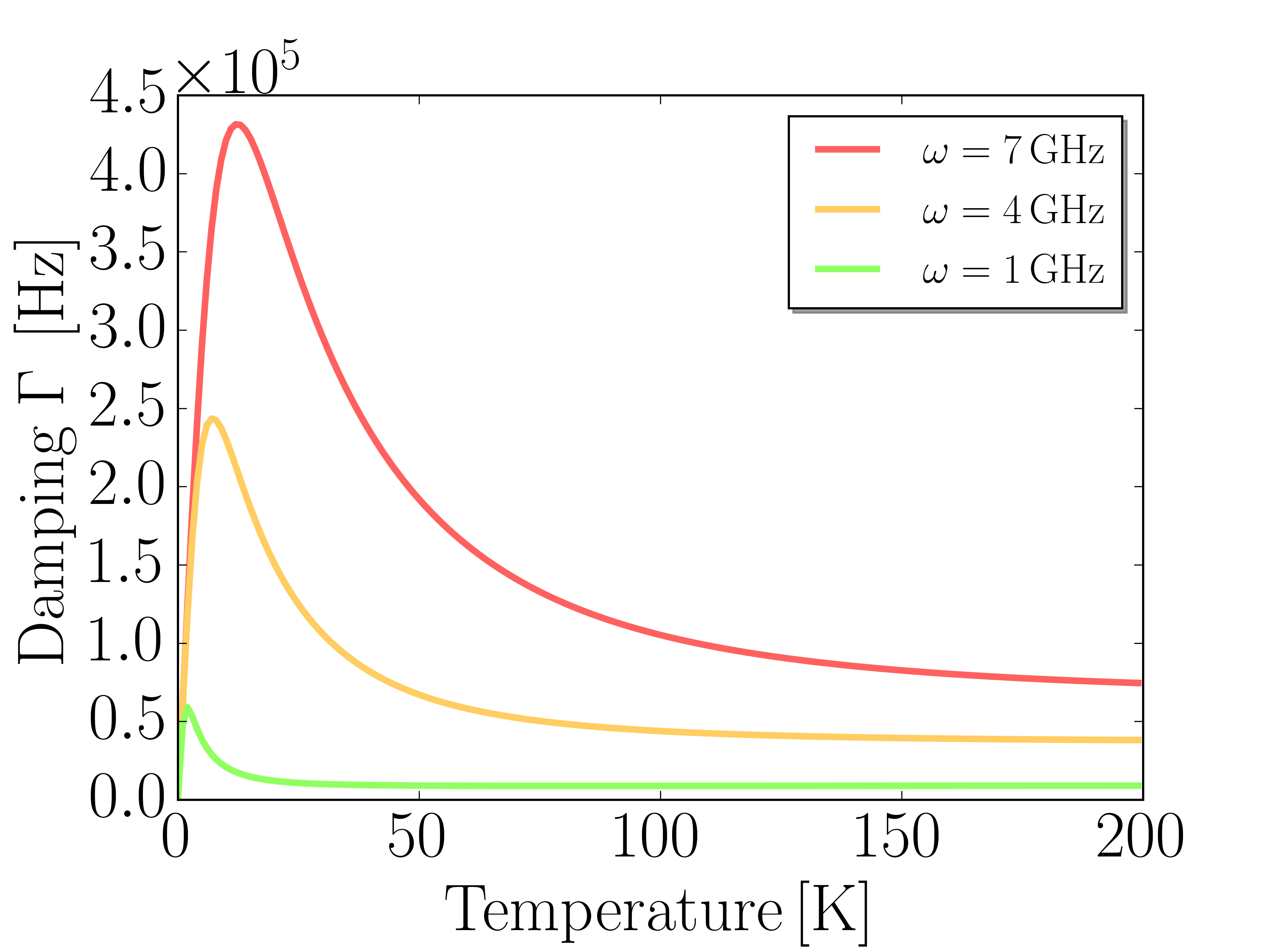
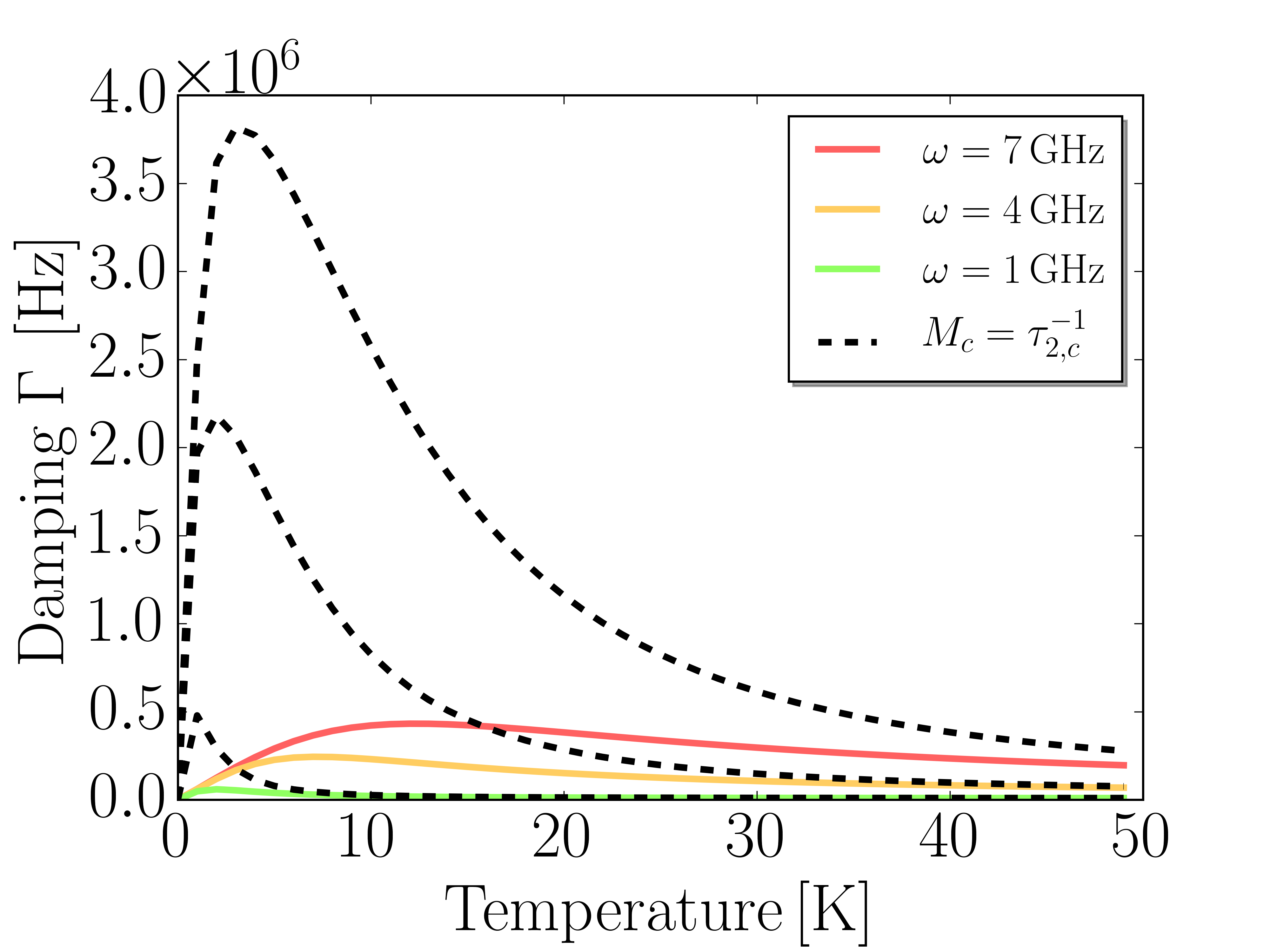
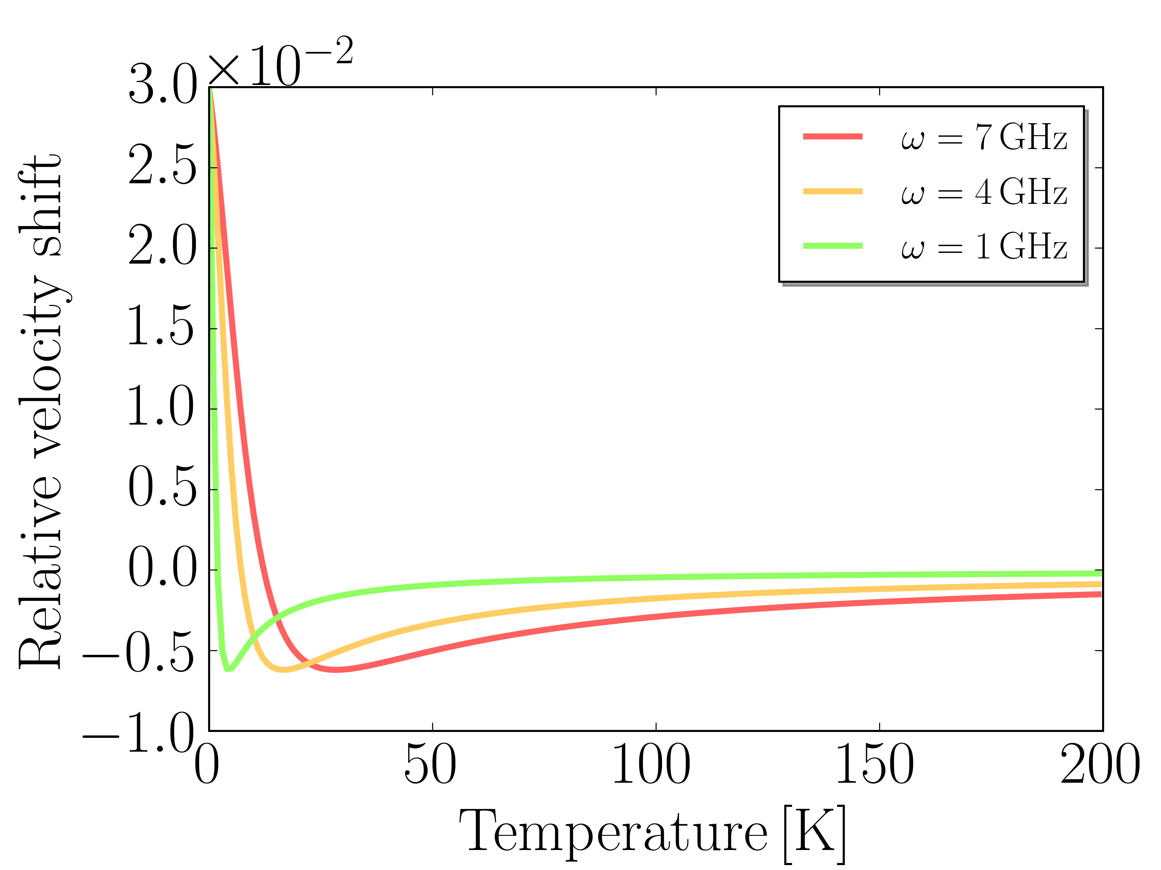
Figure 10: The Figure shows the damping coefficients and velocity shifts of LiNbO₃ surface acoustic waves induced by a graphene sheet laying on top of the crystal. Due to the $\sim 1/T$ dependence of the scattering times $\tau_{c,m}$, changing the temperature alters the quantity $v\tau_{c,m}q$, where $q$ is the SAW wave-vector, such that the functional dependence of $\sigma_{\parallel}\left(q,\omega=v_{s}q\right)$ can be investigated without switching the SAW frequencies. Here, $v_{s}$ is the SAW velocity. Left figure: Damping coefficients of SAWs for three distinct frequencies. The induced damping is small (of the order of $1/\mathrm{cm}$). Middle figure: The damping coefficients at low temperatures depend sensitively on the scattering in higher angular harmonic channels. Setting $M_{c}=\tau_{c,2}^{-1}$, thus neglecting the scattering times $\tau_{c,m>2}$, raises the damping by an order of magnitude. Right figure: Upper right pannel: Relative velocity shifts $\Delta v_{s}/v_{s}$. The velocity shifts are large (on the order of $1\%$). This is a consequence of the mainly capacitive behavior of the graphene sheet at small frequencies (see main text).

VII Poiseuille profiles

The wave-vector-dependence of transport coefficients is of importance when the currents in a system are spatially inhomogeneous, either because the applied fields are inhomogeneous, or because the inhomogeneity is imposed by the geometry of the system. The simplest example for the latter case is the Poiseuille flow. In undoped graphene, the energy current is conserved due to the conservation of momentum, however it is dissipated by the uneven boundaries of the sample Kiselev2019b . In a Poiseuille geometry, which consists of an infinitely long, straight sample of width $w$, the boundaries slow down the current flow. The current profile becomes parabolic across the sample. On the other hand, charge currents decay in the bulk of undoped graphene due to the interaction induced resistivity. In this case, there exists a crossover from an almost flat current profile if $w\gg v\tau_{c,1}$ to a more parabola-like shape at $w<v\tau_{c,1}$. However, as shown in Ref. Kiselev2019b , the slowing down of the flow by the boundaries becomes inefficient when $w\lesssim v\tau_{c,2}$, again changing the profile. In this section we investigate the Poiseuille profiles of charge currents in undoped graphene using the full non-local conductivity (64).

VII.1 Flow equations and boundary conditions

The thermal and charge flow is governed by the constitutive relations

$$\kappa^{-1}\left(\mathbf{q},\omega\right)_{\alpha\beta}j_{\varepsilon,\beta}=-\partial_{\alpha}T$$ (90)

and

$$\sigma^{-1}\left(\mathbf{q},\omega\right)_{\alpha\beta}j_{c,\beta}=E_{\alpha},$$ (91)

where $j_{\varepsilon,\beta}$ is the thermal current and $j_{c,\beta}$ the electric current. With the thermal and electric conductivities $\kappa$ and $\sigma$ depending on the wave vector $\mathbf{q}$, these equations can be seen as Fourier transforms of differential equations. Similar equations have been studied to describe non-localities induced by vortices in type II superconductors Huse1993 . The temperature gradient $-\partial_{\alpha}T$ and the electric field $E_{\alpha}$ act as source terms. In a Poiseuille geometry, the force fields act perpendicular to the gradient of the flow velocity, i.e. it is $\mathbf{E}\perp\mathbf{q}$, $\nabla T\perp\mathbf{q}$. Therefore, the currents are determined by the transverse conductivities. Let the sample be oriented in $y$-direction and centered around $x=0$. The equations then read

$$\kappa_{T}^{-1}\left(q_{x},\omega\right)j_{\varepsilon,y}\left(q_{x},\omega\right) =-\partial_{y}T,$$ (92)

$$\sigma_{T}^{-1}\left(q_{x},\omega\right)j_{c,y}\left(q_{x},\omega\right) =E_{y}.$$ (93)

To solve the above equations, boundary conditions at the sample boundaries at $\pm w/2$ are needed. As discussed in Ref. Kiselev2019a , partial slip boundary conditions are appropriate:

$$j_{\varepsilon/c,y}\left(x=\pm w/2,\omega\right)=\mp\zeta\left.\frac{\partial j_{\varepsilon/c,y}}{\partial x}\right|_{x=\pm w/2}.$$ (94)

$\zeta$ is the so called slip length parameterizing the momentum charge (current) dissipation at the sample boundaries. If the boundaries are sufficiently rough, $\zeta$ is of the order of the mean free path associated with the $m=2$ scattering time: $\zeta\sim v\tau_{\varepsilon/c,2}$. In principle, the Eqs. (92), (93) represent infinite order differential equations and require infinitely many boundary conditions. However, this problem does not appear explicitly in the calculation. The finite width of the sample $w$ sets a natural cut-off for the wave-numbers $q$, and therefore only the low powers of $q$ are relevant on the right hand side of Eqs. (92), (93). For simplicity, the boundary condition (94) is used, which is reasonable for not too small widths.

The Eqs. (92), (93) now can be solved by performing a Fourier transform. To fix the boundary conditions two point-like delta-function inhomogeneities are positioned at $\pm w$. In real space the equations take the form

$$\kappa_{T}^{-1}\left(\partial_{x},\omega\right)j_{\varepsilon,y}\left(x,\omega\right) =-\partial_{y}T-\alpha\delta\left(x-w\right)-\beta\delta\left(x+w\right)$$ (95)

$$\sigma_{T}^{-1}\left(\partial_{x},\omega\right)j_{c,y}\left(x,\omega\right) =E_{y}-\alpha\delta\left(x-w\right)-\beta\delta\left(x+w\right).$$ (96)

If the constants $\alpha$, $\beta$ are chosen such that Eq. (94) is satisfied, the solution inside the sample will be identical to the solution of the homogeneous equations with the matching boundary conditions.

Here, the profiles of electric current flows through samples of different widths will be calculated. Solving the Eq. (95) in Fourier space one obtains

$$j_{c,y}\left(q_{x},\omega\right)=$$

$$\qquad\left(2\pi E_{y}\delta\left(q_{x}\right)-\alpha e^{-iwq_{x}}-\beta e^{iwq_{x}}\right)\sigma_{T}\left(q_{x},\omega\right).$$ (97)

Inserting this result into Eq. (94) gives two algebraic equations, from which $\alpha$ and $\beta$ can be determined:

$$\zeta\int\frac{dq_{x}}{2\pi}\left(iq_{x}\right)\left(\alpha e^{-iq_{x}\frac{3w}{2}}+\beta e^{iq_{x}\frac{w}{2}}\right)\sigma_{T}\left(q_{x},\omega\right)=$$

$$\qquad\int\frac{dq_{x}}{2\pi}\left(\alpha e^{-iq_{x}\frac{3w}{2}}+\beta e^{iq_{x}\frac{w}{2}}\right)\sigma_{T}\left(q_{x},\omega\right)-$$

$$\qquad\qquad E_{y}\sigma_{T}\left(0,\omega\right)$$

$$\zeta\int\frac{dq_{x}}{2\pi}\left(iq_{x}\right)\left(\alpha e^{-iq_{x}\frac{w}{2}}+\beta e^{iq_{x}\frac{3w}{2}}\right)\sigma_{T}\left(q_{x},\omega\right)=$$

$$\qquad-\int\frac{dq_{x}}{2\pi}\left(\alpha e^{-iq_{x}\frac{w}{2}}+\beta e^{iq_{x}\frac{3w}{2}}\right)\sigma_{T}\left(q_{x},\omega\right)+$$

$$\qquad\qquad E_{y}\sigma_{T}\left(0,\omega\right).$$

The above integrals are calculated with the FFT algorithm. Once $\alpha$, $\beta$ are found, a Fourier transform the of the solution (97) gives the desired flow profiles.

Figs. 11 and 12 show the results for different widths $w$. For demonstration purposes no-slip boundary conditions ($\zeta=0$) were assumed in Fig. 11. Here, for $w>v\tau_{c,1}$ the flow profile turns flat in the middle of the sample and steeply descends to zero at the boundaries (as necessitated by the no-slip boundary conditions). This behavior is due to the interaction-induced conductivity that dissipates current uniformly across the sample - at a distance $d>v\tau_{c,1}$ away from the boundary, a uniform flow is restored. On the other hand, for $w<v\tau_{c,1}$ the current-relaxing scattering processes in the $m=1$ channel become less and less important. The scattering in the $m=2$ channel dominates. It acts in the same way viscous forces act in ordinary flows. Current is transported from the middle of the sample, where it is maximal, to the sample edges, where it is dissipated. A finite slip length (as discussed, $\zeta=v\tau_{c,2}$ was chosen for simplicity) alters these results (see Fig. 12): Whereas for widths $w>v\tau_{c,1}$ the finite slip gives the current a non-negligible velocity at the sample boundary, for small widths $w<v\tau_{c,2}$, the flow profiles are rendered flatter, and the boundary effects become negligible. In the crossover region $w\sim v\tau_{c,1}$, the profiles are curved and resemble a parabola. This takes place around $w\sim 0.5v\tau_{c,2}$ and is in accordance with the general expectations Kiselev2019a : for $w<v\tau_{c,2}$ the quasi-viscous transport of currents from the middle of the sample towards the boundaries becomes inefficient, and the boundary does efficiently dissipate the current.

Figure 11: Poiseuille profiles of charge currents in undoped graphene samples of different widths $w$. Although physically incorrect, no-slip boundary conditions were assumed for clarity. The profiles are normalized to the current at $x=0$. At large widths $w>v\tau_{c,1}$, the flow profiles turn flat. In the bulk they resemble Ohmic flow. For small widths $w<v\tau_{c,1}$, the momentum non-conserving scattering becomes inefficient. The electrons travel a distance corresponding to several width before loosing their momentum. Consequently, the profiles take a parabolic form, resembling classical Poiseuille flow. The profiles were calculated from Eq. (97).

Figure 12: Poiseuille profiles of charge currents in undoped graphene samples of different widths $w$, normalized to the current at $x=0$. Partial slip boundary conditions with a slip length $\zeta=v\tau_{c,2}$ were applied. At very small widths $w\ll\zeta$, boundary scattering ceases to be an efficient mechanism for the dissipation of electric current. The profiles turn flat, as they do in the nearly Ohmic regime $w>v\tau_{c,1}$. In the crossover regime at widths $w\sim 0.5v\tau_{c,1}$, profile curvature is most pronounced. The profiles were calculated from Eq. (97).

An interesting question is how the collective modes investigated in Sec. V are changed when the Dirac fluid is confined to a Poiseuille type sample with the boundary conditions of Eq. (94). For large sample sizes one can expect that e.g. the charge modes will exhibit a small correction of the order of $l_{c,1}/w$. The effects for small $w$ should be more interesting. They are, however, beyond the scope of the present study.

VIII Conclusion

In conclusion we have developed a kinetic theory of non-local charge and thermal transport in a clean Dirac fluid in the hydrodynamic regime. We obtained closed analytic expressions for the frequency and wave-vector-dependent, charge and thermal conductivities as well as the non-local viscosity due to electron-electron Coulomb interactions. Our solution is possible due to the dominance of so-called colinear zero modes. In the limit os a small fine-structure constant of graphene, all other mode relax more rapidly, limiting the phase space of the collective excitations that dominate the long-time dynamics. One aspect of the same physics, that was discussed previously by us in Ref.Kiselev2019b , is the onset of superdiffusion in phase space, where Lévy-flight behavior on the Dirac cone emerges. Frequent small angle scattering events are interrupted by rate large-angle scattering processes. We made specific predictions for measurements such as the velocity shift of surface acoustic waves and for inhomogeneous flow pattern. Those become identical to the one that follow from the solution of the Navier-Stokes equations in the long wavelength limit, but include higher order gradients that come into play as the sample geometry becomes smaller. In particular, we have demonstrated how the non-local transport coefficients determine the profiles of a hydrodynamic flow through narrow channels. In addition we determined the collective mode spectrum of the system including plasma waves and second sound like thermal waves. We find a complex structure of damped collective excitations. These excitations are similar to the so-called “non-hydrodynamic” modes that were shown to be relevant for the equilibration of other collission-domuinated quantum fluids Brewer2015 Romatschke2016 ; Romatschke2018 ; Heller2018 .

Appendix A The collision operator

Transformed to the band basis, the interaction part of the Hamilton operator (8) reads

$$H_{{\rm int}}=\frac{1}{2}\int_{k,k^{\prime},q}\sum_{\alpha\beta}T_{\lambda\mu\mu^{\prime}\lambda^{\prime}}\left(\mathbf{k,k}^{\prime},\mathbf{q}\right)\psi_{\lambda^{\prime}}^{\dagger}\left(\mathbf{k+q},t\right)\psi_{\mu}^{\dagger}\left(\mathbf{k}^{\prime}-\mathbf{q},t\right)\psi_{\mu^{\prime}}\left(\mathbf{k}^{\prime},t\right)\psi_{\lambda}\left(\mathbf{k,}t\right)$$ (98)

where the matrix elements $T_{\lambda\mu\mu^{\prime}\lambda^{\prime}}\left(\mathbf{k,k}^{\prime},\mathbf{q}\right)$

$$T_{\lambda\mu\mu^{\prime}\lambda^{\prime}}\left(\mathbf{k,k}^{\prime},\mathbf{q}\right)=V\left(q\right)\left(U_{\mathbf{k+q}}U_{\mathbf{k}}^{-1}\right)_{\lambda^{\prime}\lambda}\left(U_{\mathbf{k}^{\prime}-\mathbf{q}}U_{\mathbf{k}^{\prime}}^{-1}\right)_{\mu\mu^{\prime}}.$$ (99)

$U$ is the usual transformation from sub-lattice space to the band space (see Eq. 11). For the derivation of the quantum Boltzmann equation, the self energies $\Sigma{}_{\lambda}^{\gtrless}$ and the Green’s functions $g_{\lambda^{\prime}}^{\gtrless}$ are of interest (the small $g$ is used for the Green’s function transformed to the band basis $g^{\gtrless}\left(\mathbf{X},T;\mathbf{k},\omega\right)=U_{\mathbf{k}}G^{\gtrless}\left(\mathbf{X},T;\mathbf{k},\omega\right)U_{\mathbf{k}}^{\dagger}$, where $\left(\mathbf{X},T\right)$ are the center of mass coordinates, and $\left(\mathbf{k},\omega\right)$ are the relative coordinates after the Wigner transform). For details on the Wigner transform and the definitions of $G^{\gtrless}$, $\Sigma{}^{\gtrless}$ see e.g. Kita2010 ; KadanoffBaym ; Mahan ). The off diagonal elements of greens functions in band space can be neglected if the frequencies of interest are smaller than the energies of thermally excited particles: $\omega\ll k_{B}T$. In the following, only the weak space and time dependencies induced by external forces and represented by the center of mass coordinates will be of interest. For simplicity, the dependence on $\left(\mathbf{X},T\right)$ will be suppressed. The Green’s functions $g_{\lambda^{\prime}}^{\gtrless}\left(\mathbf{k},\omega\right)$ can be related to the distribution function:

$$g_{\lambda}^{>}\left(\mathbf{k},\omega\right) = -i2\pi\delta\left(\omega-\varepsilon_{\lambda}\left(\mathbf{k}\right)-U_{\mathrm{pot}}\right)\left(1-f_{\lambda,\mathbf{k}}\left(\omega\right)\right)$$

$$g_{\lambda}^{<}\left(\mathbf{k},\omega\right) = i2\pi\delta\left(\omega-\varepsilon_{\lambda}\left(\mathbf{k}\right)-U_{\mathrm{pot}}\right)f_{\lambda,\mathbf{k}}\left(\omega\right).$$ (100)

To second order in perturbation theory, for the self-energies

$$\Sigma{}_{\lambda}^{\gtrless}\left(\mathbf{k,}\omega\right) = N\sum_{\mu\mu^{\prime}\lambda^{\prime}}\int\frac{d^{2}qd^{2}k^{\prime}d\omega_{1}d\omega_{2}}{\left(2\pi\right)^{6}}\left|T_{\lambda\mu\mu^{\prime}\lambda^{\prime}}\left(\mathbf{k,k}^{\prime},\mathbf{q}\right)\right|^{2}$$ (101)

$$\times g_{\lambda^{\prime}}^{\gtrless}\left(\mathbf{k+q,}\omega_{1}\right)g_{\mu}^{\gtrless}\left(\mathbf{k}^{\prime}-\mathbf{q,}\omega_{2}\right)g_{\mu^{\prime}}^{\lessgtr}\left(\mathbf{k}^{\prime}\mathbf{,}\omega_{1}+\omega_{2}-\omega\right)$$

$$- \sum_{\mu\mu^{\prime}\lambda^{\prime}}\int\frac{d^{2}qd^{2}k^{\prime}}{\left(2\pi\right)^{4}}\int\frac{d\omega_{1}d\omega_{2}}{\left(2\pi\right)^{2}}T_{\lambda\lambda^{\prime}\mu^{\prime}\mu}\left(\mathbf{k,k}^{\prime},\mathbf{k}^{\prime}-\mathbf{q-k}\right)T_{\lambda\mu\mu^{\prime}\lambda^{\prime}}\left(\mathbf{k,k}^{\prime},\mathbf{q}\right)^{\ast}$$

$$\times g_{\lambda^{\prime}}^{\gtrless}\left(\mathbf{k+q,}\omega_{1}\right)g_{\mu}^{\gtrless}\left(\mathbf{k}^{\prime}-\mathbf{q,}\omega_{2}\right)g_{\mu^{\prime}}^{\lessgtr}\left(\mathbf{k}^{\prime}\mathbf{,}\omega_{1}+\omega_{2}-\omega\right)$$

holds. $N=4$ accounts for the spin-valley degeneracy.

The collision operator, as it appears in Eq. (12), can now be determined from the self energies $\Sigma^{<}$ and $\Sigma^{>}$. It can then be written in terms of the distribution function $f_{\lambda}\left(\mathbf{k}\right)$:

$${\cal C}_{\lambda}\left(\mathbf{k}\right)=-i\Sigma_{\lambda}^{<}\left(\mathbf{k},\varepsilon_{\lambda}\left(\mathbf{k}\right)\right)\left(1-f_{\lambda}\left(\mathbf{k}\right)\right)-i\Sigma_{\lambda}^{>}\left(\mathbf{k},\varepsilon_{\lambda}\left(\mathbf{k}\right)\right)f_{\lambda}\left(\mathbf{k}\right).$$ (102)

The delta function $\delta\left(\omega-\varepsilon_{\lambda}\left(\mathbf{k}\right)-U_{\mathrm{pot}}\left(\mathbf{x}\right)\right)$ sets the left hand side of the quantum Boltzmann equation to zero and therefore cancels out. Inserting Eqs. (100) into the self energies, parameterizing the deviations of $f_{\lambda}\left(\mathbf{k}\right)$ from the equilibrium distribution function as shown in Eq. (14), and linearizing in $\psi_{\mathbf{k}\lambda}\left(\mathbf{x},t\right)$ leads to the collision operator of Eq. (III.1). The matrix elements $\gamma_{\mathbf{k},\mathbf{k}^{\prime},\mathbf{q}}^{\left(1,2\right)}$ of Eq. (III.1) are given by:

$$\gamma_{1}\left(\mathbf{k,k}^{\prime},\mathbf{q}\right) = \left(N-1\right)\left|T_{A}\left(\mathbf{k,k}^{\prime},\mathbf{q}\right)\right|^{2}+\frac{1}{2}\left|T_{A}\left(\mathbf{k,k}^{\prime},\mathbf{k}^{\prime}-\mathbf{q-k}\right)-T_{A}\left(\mathbf{k,k}^{\prime},\mathbf{q}\right)\right|^{2}$$

$$-\left|T_{A}\left(\mathbf{k,k}^{\prime},\mathbf{k}^{\prime}-\mathbf{q-k}\right)\right|^{2}$$

$$\gamma_{2}\left(\mathbf{k,k}^{\prime},\mathbf{q}\right) = \left(N-1\right)\left|T_{B}\left(\mathbf{k,\mathbf{k}^{\prime}},\mathbf{\mathbf{k}^{\prime}-k-\mathbf{q}}\right)\right|^{2}+\left(N-1\right)\left|T_{A}\left(\mathbf{k,\mathbf{k}^{\prime}},\mathbf{q}\right)\right|^{2}$$ (103)

$$+\left|T_{A}\left(\mathbf{k,\mathbf{k}^{\prime}},\mathbf{q}\right)-T_{B}\left(\mathbf{k,\mathbf{k}^{\prime}},\mathbf{\mathbf{k}^{\prime}-\mathbf{q}}\mathbf{-k}\right)\right|^{2},$$

with

$$T_{A}\left(\mathbf{k,k}^{\prime},\mathbf{q}\right) = T_{++++}\left(\mathbf{k,k}^{\prime},\mathbf{q}\right)=T_{----}\left(\mathbf{k,k}^{\prime},\mathbf{q}\right)$$

$$= T_{+--+}\left(\mathbf{k,k}^{\prime},\mathbf{q}\right)=T_{-++-}\left(\mathbf{k,k}^{\prime},\mathbf{q}\right)$$

$$= \frac{V\left(q\right)}{4}\left(1+\frac{\left(K+Q\right)K^{\ast}}{\left|\mathbf{k+q}\right|k}\right)\left(1+\frac{\left(K^{\prime}-Q\right)K^{\prime\ast}}{\left|\mathbf{k}^{\prime}\mathbf{-q}\right|k^{\prime}}\right)$$

and

$$T_{B}\left(\mathbf{k,k}^{\prime},\mathbf{q}\right) = T_{++--}\left(\mathbf{k,k}^{\prime},\mathbf{q}\right)=T_{--++}\left(\mathbf{k,k}^{\prime},\mathbf{q}\right)$$ (104)

$$= \frac{V\left(q\right)}{4}\left(1-\frac{\left(K+Q\right)K^{\ast}}{\left|\mathbf{k+q}\right|k}\right)\left(1-\frac{\left(K^{\prime}-Q\right)K^{\prime\ast}}{\left|\mathbf{k}^{\prime}\mathbf{-q}\right|k^{\prime}}\right)$$

Upper-case letters like $K=k_{x}+ik_{y}$ etc. combine the two components of the momentum vector onto a complex variable.

Since the quantum Boltzmann equation only accounts for the diagonal in $\lambda$ components of the distribution function, the currents also have to be decomposed into contributions that involve particle-hole pair creation $\left(\mathbf{j}_{\mathrm{inter}}\right)$ and those who do not $\left(\mathbf{j}_{\mathrm{intra}}\right)$. Here, the identity

$$U_{\mathbf{k}}\mathbf{\sigma}U_{\mathbf{k}}^{-1}=\frac{\mathbf{k}}{k}\sigma_{z}-\frac{\mathbf{k\times e}_{z}}{k}\sigma_{y}$$ (105)

is useful. The charge current

$$\mathbf{j}_{c}=ev\int_{\mathbf{k}}\psi^{\dagger}\left(\mathbf{k}\right)\mathbf{\sigma}\psi\left(\mathbf{k}\right)$$ (106)

can be written as

$$\mathbf{j}_{c}=\mathbf{j}_{c,\mathrm{intra}}+\mathbf{j}_{c,\mathrm{inter}},$$ (107)

where the two contributions are given by

$$\mathbf{j}_{c,\mathrm{intra}} = ev\int_{\mathbf{k}}\sum_{\lambda=\pm}\frac{\lambda\mathbf{k}}{k}\gamma_{\mathbf{k},\lambda}^{\dagger}\gamma_{\mathbf{k},\lambda}$$

$$\mathbf{j}_{c,\mathrm{inter}} = iev\int_{\mathbf{k}}\frac{\mathbf{k\times e}_{z}}{k}\left(\gamma_{\mathbf{k},+}^{\dagger}\gamma_{\mathbf{k},-}-\gamma_{\mathbf{k},-}^{\dagger}\gamma_{\mathbf{k},+}\right).$$ (108)

The energy current $\mathbf{j}_{\varepsilon}$ and the momentum current tensor $\tau_{xy}$ can be decomposed in a similar manner. This leads to the expressions (47) and (48) of the main text and the expression that is used for $\tau_{xy}$ in Sec. IV.3.3. As discussed above, in the hydrodynamic regime, it is legitimate to focus on the intra-band contributions, which dominate the transport behavior of the system.

Appendix B Collinear scattering and collinear zero modes

Here, the logarithmic divergence of the collision operator for collinear processes is demonstrated following Ref. Fritz2008 . We then show, that the $m$-dependent collinear zero modes are those given in Eq. (32).

The essential mathematics behind the divergence is contained in phase space density available for two particle collisions. The phase space is restricted by the delta function ensuring energy conservation: $\delta\left(k+k_{1}-\left|\mathbf{k}+\mathbf{q}\right|-\left|\mathbf{k}_{1}-\mathbf{q}\right|\right)$. This can be seen from power counting in Eq. (III.1) using Eqs. (103), (104).

Choosing $\mathbf{k}=\left(k,0\right)$ with $k>0$, and writing $\mathbf{k}_{1}=\left(k_{1},k_{\bot}\right),$ $\mathbf{q}=\left(q,q_{\bot}\right)$, collinear scattering occurs when $k_{1}>0$, $k+q>0$, $k_{1}-q>0$ and $q_{\bot}\approx 0$, $k_{\bot}\approx 0$. For small $q_{\bot}$, $k_{\bot}$ the argument of the delta function can be approximated as

$$k+k_{1}-\left|\mathbf{k}+\mathbf{q}\right|-\left|\mathbf{k}_{1}-\mathbf{q}\right|\approx\frac{k_{\bot}^{2}}{2k_{1}}-\frac{q_{\bot}^{2}}{2\left(k+q\right)}-\frac{\left(k_{\bot}-q_{\bot}\right)^{2}}{2\left(k_{1}-q\right)}.$$ (109)

The right hand side of this equation is a polynomial in $q_{\bot}$, and can be written in terms of linear factors as

$$\frac{k_{\bot}^{2}}{2k_{1}}-\frac{q_{\bot}^{2}}{2\left(k+q\right)}-\frac{\left(k_{\bot}-q_{\bot}\right)^{2}}{2\left(k_{1}-q\right)}=-\frac{k_{1}+k}{2\left(k+q\right)\left(k_{1}-q\right)}\left(q_{\bot}-\zeta_{1}k_{\bot}\right)\left(q_{\bot}-\zeta_{2}k_{\bot}\right).$$

It is then easy to see by performing the $q_{\bot}$ integration that

$$\int dk_{\bot}dq_{\bot}\delta\left(-\frac{k_{1}+k}{2\left(k+q\right)\left(k_{1}-q\right)}\left(q_{\bot}-\zeta_{1}k_{\bot}\right)\left(q_{\bot}-\zeta_{2}k_{\bot}\right)\right)\propto\int\frac{dk_{\bot}}{k_{\bot}}.$$

This behavior leads to a logarithmic divergence. The divergence is however cut off by the screening of the Coulomb potential Mueller2008

$$V\left(\left|\mathbf{q}\right|\right)\rightarrow V\left(\left|\mathbf{q}\right|+q_{TF}\right),$$

where $q_{TF}$ is the Thomas Fermi screening length. In the case of charge neutral graphene $q_{FT}=\alpha k_{B}T/v$. If the screening is included, the integral of (III.1) vanishes in the infrared. Thus, the contribution of collinear processes to the scattering rates is enhanced by the large factor

$$\log\left(1/\alpha\right).$$

It was demonstrated in sec. III.2 of the main text, that relaxation processes in the hydrodynamic regime are dominated by collinear zero modes. As demonstrated above, these modes describe scattering events in which all particle velocities show in the same direction. Examining the delta function responsible for energy conservation $\delta\left(k+k_{1}-\left|\mathbf{k}+\mathbf{q}\right|-\left|\mathbf{k}_{1}-\mathbf{q}\right|\right)$, we see that, if all momenta are parallel to each other, energy is only conserved, if the above conditions $k>0$, $k_{1}>0$, $k+q>0$, $k_{1}-q>0$ apply (except for unimportant isolated points in phase space). The exchange momentum $q$, however, can be positive or negative. To find those $\psi_{\mathbf{k}\lambda}$ that correspond to collinear zero modes, two terms in the collision operator Eq. (III.1) have to be considered:

$$A_{\mathbf{k},\mathbf{k}_{1},\mathbf{q},\lambda}^{\left(1\right)} = \psi_{\mathbf{k}+\mathbf{q}\lambda}+\psi_{\mathbf{k}_{1}-\mathbf{q}\lambda}-\psi_{\mathbf{k}_{1}\lambda}-\psi_{\mathbf{k}\lambda}$$

$$A_{\mathbf{k},\mathbf{k}_{1},\mathbf{q},\lambda}^{\left(2\right)} = \psi_{\mathbf{k}+\mathbf{q}\lambda}-\psi_{-\mathbf{k}_{1}+\mathbf{q}\bar{\lambda}}+\psi_{-\mathbf{k}_{1}\bar{\lambda}}-\psi_{\mathbf{k}\lambda}.$$ (110)

Using the parameterization

$$\psi_{\mathbf{k},\lambda}=a_{\lambda,m}\left(k\right)e^{im\theta_{\mathbf{k}}}$$ (111)

yields

$$A_{\mathbf{k},\mathbf{k}^{\prime},\mathbf{q},\lambda}^{\left(1\right)} = \left(a_{\lambda,m}\left(k+q\right)+a_{\lambda,m}\left(k_{1}-q\right)-a_{\lambda,m}\left(k_{1}\right)-a_{\lambda,m}\left(k\right)\right)e^{im\theta_{\mathbf{k}}}$$

$$A_{\mathbf{k},\mathbf{k}^{\prime},\mathbf{q},\lambda}^{\left(2\right)} = \left(a_{\lambda,m}\left(k+q\right)-\left(-1\right)^{m}a_{\bar{\lambda},m}\left(k_{1}-q\right)+\left(-1\right)^{m}a_{\bar{\lambda},m}\left(k_{1}\right)-a_{\lambda,m}\left(k\right)\right)e^{im\theta_{\mathbf{k}}}.$$ (112)

For collinear zero modes

$$A_{\mathbf{k},\mathbf{k}^{\prime},\mathbf{q},\lambda}^{\left(1\right)} = 0$$

$$A_{\mathbf{k},\mathbf{k}^{\prime},\mathbf{q},\lambda}^{\left(2\right)} = 0$$

has to hold. $A_{\mathbf{k},\mathbf{k}^{\prime},\mathbf{q},\lambda}^{\left(1\right)}$ is set to zero by $a_{\lambda,m}\left(k\right)=\left\{1,\lambda,\beta v\hbar k,\lambda\beta v\hbar k\right\}$. $A_{\mathbf{k},\mathbf{k}^{\prime},\mathbf{q},\lambda}^{\left(2\right)}$ is more restrictive. For even $m$ its zero modes are given by $a_{\lambda,m}\left(k\right)=\left\{1,\lambda,\lambda\beta v\hbar k\right\}$, for odd $m$ the zero modes are $a_{\lambda,m}\left(k\right)=\left\{1,\lambda,\beta v\hbar k\right\}$. Summing up, the collinear zero modes are given by

$$a_{\lambda,m}=\lambda^{m}\left\{1,\lambda,\lambda\beta v\hbar k\right\}e^{im\theta_{\mathbf{k}}}.$$

Appendix C Matrix elements of the collision operator

The values of some matrix elements are shown in Table 1. For $m\geq 2$ the values can be approximated by

$$\left\langle\chi_{\mathbf{k},\lambda}^{\left(m,s=1\right)}\left|\mathcal{C}\right|\chi_{\mathbf{k},\lambda}^{\left(m,s=1\right)}\right\rangle = 2.574\cdot\left|m\right|-3.456$$

$$\left\langle\chi_{\mathbf{k},\lambda}^{\left(m,s=2\right)}\left|\mathcal{C}\right|\chi_{\mathbf{k},\lambda}^{\left(m,s=2\right)}\right\rangle = 1.825\cdot\left|m\right|-2.741$$

$$\left\langle\chi_{\mathbf{k},\lambda}^{\left(m,s=3\right)}\left|\mathcal{C}\right|\chi_{\mathbf{k},\lambda}^{\left(m,s=3\right)}\right\rangle = 5.184\cdot\left|m\right|-11.37$$

$$\left\langle\chi_{\mathbf{k},\lambda}^{\left(m,s=2\right)}\left|\mathcal{C}\right|\chi_{\mathbf{k},\lambda}^{\left(m,s=3\right)}\right\rangle = 2.042\cdot\left|m\right|-4.398.$$

All values are given in units of $\frac{1}{v^{2}\beta^{3}\hbar^{3}}.$

$m$	$s$	$s^{\prime}$	$\left\langle\chi_{\mathbf{k},\lambda}^{\left(m,s\right)}\left|\mathcal{C}\right|\chi_{\mathbf{k},\lambda}^{\left(m,s^{\prime}\right)}\right\rangle$	$m$	$s$	$s$’	$\left\langle\chi_{\mathbf{k},\lambda}^{\left(m,s\right)}\left|\mathcal{C}\right|\chi_{\mathbf{k},\lambda}^{\left(m,s^{\prime}\right)}\right\rangle$	$m$	$s$	$s$’	$\left\langle\chi_{\mathbf{k},\lambda}^{\left(m,s\right)}\left|\mathcal{C}\right|\chi_{\mathbf{k},\lambda}^{\left(m,s^{\prime}\right)}\right\rangle$
0	1	1	0	2	1	1	2.617	4	1	1	6.988
0	1	2	0	2	1	2	0	4	1	2	0
0	1	3	0	2	1	3	0	4	1	3	0
0	2	2	0	2	2	2	1.745	4	2	2	4.722
0	2	3	0	2	2	3	1.243	4	2	3	4.122
0	3	3	0	2	3	3	3.341	4	3	3	10.456
1	1	1	0.804	3	1	1	4.728	5	1	1	9.345
1	1	2	0	3	1	2	0	5	1	2	0
1	1	3	0	3	1	3	0	5	1	3	0
1	2	2	0.463	3	2	2	3.167	5	2	2	6.351
1	2	3	0	3	2	3	2.573	5	2	3	5.800
1	3	3	0	3	3	3	6.647	5	3	3	14.610

Table 1: Matrix elements of the collision operator (III.1) with respect to the collinear zero modes $\chi_{\mathbf{k},\lambda}^{\left(m,s\right)}=\lambda^{m}e^{im\theta}\left\{1,\lambda,\lambda\beta v\hbar k\right\}$. The index $m$ labels the angular harmonic and $s$ one of the modes in curved brackets.

Appendix D Decomposition of the viscosity tensor into longitudinal and transverse parts

Consider a system with a preference direction introduced by the wave-vector $\mathbf{q}$. It is useful to define the orthogonal tensor basis

$$e_{\alpha\beta}^{\left(1\right)} = \frac{q_{\alpha}q_{\beta}}{q^{2}}$$

$$e_{\alpha\beta}^{\left(2\right)} = \delta_{\alpha\beta}-\frac{q_{\alpha}q_{\beta}}{q^{2}}$$

$$e_{\alpha\beta}^{\left(3\right)} = \frac{1}{\sqrt{2}}\left(q_{\alpha}p_{\beta}+p_{\alpha}q_{\beta}\right)/\left(pq\right),$$ (114)

which is normalized according according to

$$\sum_{\alpha\beta}e_{\alpha\beta}^{\left(i\right)}e_{\alpha\beta}^{\left(j\right)}=\delta_{ij}.$$

Here it is

$$p_{\alpha}=q_{\gamma}\varepsilon_{\gamma\alpha}.$$

In this basis, the symmetric shear force tensor $X_{0,\alpha\beta}$ can be written

$$X_{0,\alpha\beta}=X^{\left(1\right)}e_{\alpha\beta}^{\left(1\right)}+X^{\left(2\right)}e_{\alpha\beta}^{\left(2\right)}+X^{\left(3\right)}e_{\alpha\beta}^{\left(3\right)}.$$ (115)

The same holds for the momentum current (stress) tensor

$$\tau_{\alpha\beta}=\tau^{\left(1\right)}e_{\alpha\beta}^{\left(1\right)}+\tau^{\left(2\right)}e_{\alpha\beta}^{\left(2\right)}+\tau^{\left(3\right)}e_{\alpha\beta}^{\left(3\right)}.$$ (116)

Since the system is fully isotropic, except for the preference direction set by $\mathbf{q}$, the response of the system to different components of $X_{0,\alpha\beta}$ can only be distinct as far as these components relate differently to the direction of $\mathbf{q}$. Eqs (115) and (116) are decompositions of the shear force and momentum current tensors into such components. The fourth rank viscosity tensor $\eta_{\alpha\beta\gamma\delta}$ is defined through the constitutive relation

$$\tau_{\alpha\beta}=\eta_{\alpha\beta\gamma\delta}X_{0,\gamma\delta}.$$

In general, such a tensor connecting the quantities $\tau_{\alpha\beta}$ and $X_{0,\alpha\beta}$ as given by Eqs. (115), (116) can be written as $\eta_{\alpha\beta\gamma\delta}=\sum_{ij}e_{\alpha\beta}^{\left(i\right)}e_{\gamma\delta}^{\left(j\right)}\eta^{\left(ij\right)}$. However it follows from an Onsager reciprocity relation that $\eta_{\alpha\beta\gamma\delta}$ has to be symmetric with respect to an interchange of the first and last pairs of indices:

$$\eta_{\left(\alpha\beta\right)\left(\gamma\delta\right)}=\eta_{\left(\gamma\delta\right)\left(\alpha\beta\right)}.$$

This condition further restricts the form of $\eta_{\alpha\beta\gamma\delta}$ to

$$\eta_{\alpha\beta\gamma\delta}=\sum_{i}e_{\alpha\beta}^{\left(i\right)}e_{\gamma\delta}^{\left(i\right)}\eta^{\left(i\right)}.$$ (117)

Calculating the scalars $\eta^{\left(i\right)}$ using the quantum Boltzmann equation, one finds $\eta^{\left(1\right)}=\eta^{\left(2\right)}\neq\eta^{\left(3\right)}$. For reasons explained in the main text, we call $\eta^{\left(1\right)}=\eta^{\left(2\right)}=\eta_{\perp}$ the transverse, and $\eta^{\left(3\right)}=\eta_{\parallel}$ the longitudinal viscosity. In the sense that $\eta_{\alpha\beta\gamma\delta}$ is spanned by projection operators onto the tensorial subspaces which span the force and current tensors and are given in Eqs. (114), the decomposition (117) is completely analogous to the decomposition of a conductivity tensor into transverse and longitudinal parts (see Eq. (63)).

References

- (1) E. I. Kiselev and J. Schmalian, Lévy flights and hydrodynamic superdiffusion on the dirac cone of graphene, Phys. Rev. Lett. 123, 195302 (2019).
- (2) A. B. Pippard, The surface impedance of superconductors and normal metals at high frequencies. ii. the anomalous skin effect in normal metals, Proc. R. Soc. Lond. A 191, 385 (1947).
- (3) A. B. Pippard, Trapped flux in superconductors, Philosophical Transactions of the Royal Society A: Math., Phys. and Eng. Sci. 248, 97 (1955).
- (4) J. R. Waldram, A. B. Pippard, and J. Clarke, Theory of the current-voltage characteristics of sns junctions and other superconducting weak links, Philosophical Transactions of the Royal Society A: Math., Phys. and Eng. Sci. 268, 265 (1970).
- (5) D. Svintsov, Hydrodynamic-to-ballistic crossover in dirac materials, Phys. Rev. B 97, 121405 (2018).
- (6) I. Torre, L. V. de Castro, B. V. Duppen, D. B. Ruiz, F. M. Peeters, F. H. L. Koppens, and M. Polini, Acoustic plasmons at the crossover between the collisionless and hydrodynamic regimes in two-dimensional electron liquids, Phys. Rev. B 99, 144307 (2019).
- (7) J. Brewer and P. Romatschke, Nonhydrodynamic transport in trapped unitary fermi gases, Phys. Rev. Lett. 115, 190404 (2015).
- (8) P. Romatschke, Retarded correlators in kinetic theory: branch cuts, poles and hydrodynamic onset transitions, Eur. Phys. J. C 76, 352 (2016).
- (9) P. Romatschke, Relativistic fluid dynamics far from local equilibrium, Phys. Rev. Lett. 120, 12301 (2018).
- (10) M. P. Heller, A. Kurkela, M. Spalinski, and V. Svensson, Hydrodynamization in kinetic theory: Transient modes and the gradient expansion, Phys. Rev. D 97, 91503 (2018).
- (11) L. Fritz, J. Schmalian, M. Müller, and S. Sachdev, Quantum critical transport in clean graphene, Phys. Rev. B 78, 85416 (2008).
- (12) A. B. Kashuba, Conductivity of defectless graphene, Phys. Rev. B 78, 85415 (2008).
- (13) M. Müller, J. Schmalian, and L. Fritz, Graphene: A nearly perfect fluid, Phys. Rev. Lett. 103, 25301 (2009).
- (14) M. S. Foster and I. L. Aleiner, Slow imbalance relaxation and thermoelectric transport in graphene, Phys. Rev. B 79, 85415 (2009).
- (15) K. Damle and S. Sachdev, Nonzero-temperature transport near quantum critical points, Phys. Rev. B 56, 8714 (1997).
- (16) S. A. Hartnoll, P. K. Kovtun, M. Müller, and S. Sachdev, Theory of the nernst effect near quantum phase transitions in condensed matter and in dyonic black holes, Phys. Rev. B 76, 144502 (2007).
- (17) D. E. Sheehy and J. Schmalian, Quantum critical scaling in graphene, Phys. Rev. Lett. .
- (18) J. Crossno, J. K. Shi1, K. Wang, X. Liu, A. Harzheim, A. Lucas, S. Sachdev, P. Kim, T. Taniguchi, K. Watanabe, T. A. Ohki, and K. C. Fong, Observation of the dirac fluid and the breakdown of the wiedemann-franz law in graphene, Science 351, 1058 (2016).
- (19) P. Gallagher, C.-S. Yang, T. Lyu, F. Tian, R. Kou, H. Zhang, K. Watanabe, T. Taniguchi, and F. Wang, Quantum-critical conductivity of the dirac fluid in graphene, Science 364, 158 (2019).
- (20) J. A. Sulpizio, L. Ella, A. Rozen, J. Birkbeck, D. J. Perello, D. Dutta, M. Ben-Shalom, T. Taniguchi, K. Watanabe, T. Holder, R. Queiroz, A. Principi, A. Stern, T. Scaffidi, A. K. Geim, and S. Ilani, Visualizing poiseuille flow of hydrodynamic electrons, Nature 576, 75 (2019).
- (21) D. A. Bandurin, A. V. Shytov, L. S. Levitov, R. K. Kumar, A. I. Berdyugin, M. B. Shalom, I. V. Grigorieva, A. K. Geim, and G. Falkovich, Fluidity onset in graphene, Nature Communications 9, 4533 (2018).
- (22) D. A. Bandurin, I. Torre, R. K. Kumar, M. B. Shalom, A. Tomadin, A. Principi, G. H. Auton, E. Khestanova, K. S. Novoselov, I. V. Grigorieva, L. A. Ponomarenko, A. K. Geim, and M. Polini, Negative local resistance caused by viscous electron backflow in graphene, Science 351, 1055 (2016).
- (23) A. I. Berdyugin, S. G. Xu, F. M. D. Pellegrino, R. K. Kumar, A. Principi, I. Torre, M. B. Shalom, T. Taniguchi, K. Watanabe, I. V. Grigorieva, M. Polini, A. K. Geim, and D. A. Bandurin, Measuring hall viscosity of graphene’s electron fluid, Science 364, 162 (2019).
- (24) R. K. Kumar, D. A. Bandurin, F. M. D. Pellegrino, Y. Cao, A. Principi, H. Guo, G. H. Auton, M. B. Shalom, L. A. Ponomarenko, G. Falkovich, K. Watanabe, T. Taniguchi, I. V. Grigorieva, L. S. Levitov, M. Polini, and A. K. Geim, Superballistic flow of viscous electron fluid through graphene constrictions, Nature Physics 13, 1182 (2017).
- (25) B. N. Narozhny, I. V. Gornyi, M. Titov, M. Schütt, and A. D. Mirlin, Hydrodynamics in graphene: Linear-response transport, Phys. Rev. B 91, 035414 (2015).
- (26) U. Briskot, M. Schütt, I. V. Gornyi, M. Titov, B. N. Narozhny, and A. D. Mirlin, Collision-dominated nonlinear hydrodynamics in graphene, Phys. Rev. B 92, 115426 (2015).
- (27) A. K. G. I. Torre, A. Tomadin and M. Polini, Nonlocal transport and the hydrodynamic shear viscosity in graphene, Phys. Rev. B 92, 165433 (2015).
- (28) B. N. Narozhny, I. V. Gornyi, and A. D. Mirlin, Hydrodynamic approach to electronic transport in graphene, Ann. d. Phys. 529, 1700043 (2017).
- (29) H.-Y. Xie and A. Levchenko, Negative viscosity and eddy flow of the imbalanced electron-hole liquid in graphene, Phys. Rev. B 99, 045434 (2019).
- (30) M. J. Klug, M. S. Scheurer, and J. Schmalian, Hierarchy of information scrambling, thermalization, and hydrodynamic flow in graphene, Phys. Rev. B 98, 045102 (2018).
- (31) B. N. Narozhny, Optical conductivity in graphene: Hydrodynamic regime, Phys. Rev. B 100, 115434 (2019).
- (32) J. M. Link, D. E. Sheehy, B. N. Narozhny, and J. Schmalian, Elastic response of the electron fluid in intrinsic graphene: The collisionless regime, Phys. Rev. B 98, 195103 (2018).
- (33) L. S. Levitov, A. V. Shtyk, and M. V. Feigelman, Electron-electron interactions and plasmon dispersion in graphene, Phys. Rev. B 88, 235403 (2013).
- (34) D. S. Borgnia, T. V. Phan, and L. S. Levitov, Quasi-relativistic doppler effect and non-reciprocal plasmons in graphene, arXiv:1512.09044 (2015).
- (35) B. N. Narozhny, Electronic hydrodynamics in graphene., Annals of Physics 411, 167979 (2019).
- (36) B. N. Narozhny and M. Schütt, Magnetohydrodynamics in graphene: Shear and hall viscosities, Phys. Rev. B 100, 035125 (2019).
- (37) S. Danz and B. N. Narozhny, Vorticity of viscous electronic flow in graphene, 2D Materials 7, 035001 (2020).
- (38) O. Kashuba, B. Trauzettel, and L. W. Molenkamp, Relativistic gurzhi effect in channels of dirac materials, Phys. Rev. B 97, 205129 (2018).
- (39) A. Lucas and K. C. Fong, Hydrodynamics of electrons in graphene, Journal of Physics: Condensed Matter 30, 53001 (2018).
- (40) Z. Sun, D. N. Basov, and M. M. Fogler, Universal linear and nonlinear electrodynamics of a dirac fluid, PNAS 115, 3285 (2018).
- (41) P. J. W. Moll, P. Kushwaha, N. Nandi, B. Schmidt, and A. P. Mackenzie, Evidence for hydrodynamic electron flow in , Science 351, 1061 (2016).
- (42) A. P. Mackenzie, The properties of ultrapure delafossite metals, Rep. Prog. Phys. 80, 32501 (2017).
- (43) J. Gooth, F. Menges, N. Kumar, V. Süß, C. Shekhar, Y. Sun, U. Drechsler, R. Zierold, C. Felser, and B. Gotsmann, Thermal and electrical signatures of a hydrodynamic electron fluid in tungsten diphosphide, Nat. Commun 9, 4093 (2018).
- (44) G. M. Gusev, A. D. Levin, E. V. Levinson, and A. K. Bakarov, Viscous transport and hall viscosity in a two-dimensional electron system, Phys. Rev. B 98, 161303 (2018).
- (45) A. V. Andreev, S. A. Kivelson, and B. Spivak, Hydrodynamic description of transport in strongly correlated electron systems, Phys. Rev. Lett. 106, 256804 (2011).
- (46) A. Principi and G. Vignale, Violation of the wiedemann-franz law in hydrodynamic electron liquids, Phys. Rev. Lett. 115, 056603 (2015).
- (47) P. Alekseev, A. Dmitriev, I. Gornyi, V. Kachorovskii, B. Narozhny, M. Schütt, and M. Titov, Magnetoresistance in two-component systems, Phys. Rev. Lett. 114, 156601 (2015).
- (48) P. Alekseev, Negative magnetoresistance in viscous flow of two-dimensional electrons, Phys. Rev. Lett. 117, 166601 (2016).
- (49) H. Guo, E. Ilseven, G. Falkovich, and L. S. Levitov, Higher-than-ballistic conduction of viscous electron flows, PNAS 114, 3068 (2017).
- (50) T. Scaffidi, N. Nandi, B. Schmidt, A. P. Mackenzie, and J. E. Moore, Hydrodynamic electron flow and hall viscosity, Phys. Rev. Lett. 118, 226601 (2017).
- (51) P. S. Alekseev, Magnetic resonance in a high-frequency flow of a two-dimensional viscous electron fluid, Phys. Rev. B 98, 165440 (2018).
- (52) R. Moessner, P. Surówka, and P.Witkowski, Pulsating flow and boundary layers in viscous electronic hydrodynamics, Phys. Rev. B 97, 161112 (2018).
- (53) R. Cohen and M. Goldstein, Hall and dissipative viscosity effects on edge magnetoplasmons, Phys. Rev. B 98, 235103 (2018).
- (54) I. S. Burmistrov, M. Goldstein, M. Kot, V. D. Kurilovich, and P. D. Kurilovich, Dissipative and hall viscosity of a disordered 2d electron gas, Phys. Rev. Lett. 123, 026804 (2019).
- (55) R. Moessner, N. Morales-Durán, P. Surówka, and P. Witkowski, Boundary-condition and geometry engineering in electronic hydrodynamics, Phys. Rev. B 100, 155115 (2019).
- (56) T. Zdyrski and J. McGreevy, Effects of dissipation on solitons in the hydrodynamic regime of graphene, Phys. Rev. B 99, 235435 (2019).
- (57) P. Alekseev and A. Alekseeva, Transverse magnetosonic waves and viscoelastic resonance in a two-dimensional highly viscous electron fluid, Phys. Rev. Lett. 123, 236801 (2019).
- (58) D. Svintsov, Emission of plasmons by drifting dirac electrons: A hallmark of hydrodynamic transport, Phys. Rev. B 100, 195428 (2019).
- (59) T. Holder, R. Queiroz, T. Scaffidi, N. Silberstein, A. Rozen, J. A. Sulpizio, L. Ella, S. Ilani, and A. Stern, Ballistic and hydrodynamic magnetotransport in narrow channels, Phys. Rev. B 100, 245305 (2019).
- (60) C. Q. Cook and A. Lucas, Electron hydrodynamics with a polygonal fermi surface, Phys. Rev. B 99, 235148 (2019).
- (61) F. M. D. Pellegrino, I. Torre, and M. Polini, Nonlocal transport and the hall viscosity of two-dimensional hydrodynamic electron liquids, Phys. Rev. B 96, 195401 (2017).
- (62) P. S. Alekseev, A. P. Dmitriev, I. V. Gornyi, V. Y. Kachorovskii, B. N. Narozhny, and M. Titov, Counterflows in viscous electron-hole fluid, Phys. Rev. B 98, 125111 (2018).
- (63) J. M. Link, B. N. Narozhny, E. I. Kiselev, and J. Schmalian, Out-of-bounds hydrodynamics in anisotropic dirac fluids, Phys. Rev. Lett. 120, 196801 (2018).
- (64) I. Matthaiakakis, D. R. Fernández, C. Tutschku, E. M. Hankiewicz, J. Erdmenger, and R. Meyer, Functional dependence of the hall viscosity-induced transverse voltage in two-dimensional fermi liquids, Phys. Rev. B 101, 045423 (2020).
- (65) M. Müller, L. Fritz, and S. Sachdev, Quantum-critical relativistic magnetotransport in graphene, Phys. Rev. B 78, 115406 (2008).
- (66) A. D. Mirlin and P. Wölfle, Composite fermions in the fractional quantum hall effect: Transport at finite wave vector, Phys. Rev. Lett. .
- (67) K. A. Ingebrigtsen, Surface waves in piezoelectrics, J. Appl. Phys. 40, 2681 (1969).
- (68) S. H. Simon, Coupling of surface acoustic waves to a two-dimensional electron gas, Phys. Rev. B 54, 13878 (1996).
- (69) A. L. Efros and Y. M. Galperin, Quantization of the acoustoelectric current in a two-dimensional electron system in a strong magnetic field, Phys. Rev. Lett. 41, 1959 (1990).
- (70) A. Wixforth, J. Scriba, M. Wassermeier, J. P. Kotthaus, G. Weimann, and W. Schlapp, Surface acoustic waves on , Phys. Rev. B 40, 7874 (1989).
- (71) M. Rotter, A. Wixforth, W. Ruile, D. Bernklau, and H. Riechert, Giant acoustoelectric effect in gaas/linbo3 hybrids, Appl. Phys. Lett. 73, 2128 (1998).
- (72) A. O. Govorov, A. V. Kalameitsev, M. Rotter, A. Wixforth, J. P. Kotthaus, K.-H. Hoffmann, and N. Botkin, Nonlinear acoustoelectric transport in a two-dimensional electron system, Phys. Rev. B 62, 2659 (2000).
- (73) L. Ella, A. Rozen, J. Birkbeck, M. Ben-Shalom, D. Perello, J. Zultak, T. Taniguchi, K. Watanabe, A. K. Geim, S. Ilani, and J. A. Sulpizio, Simultaneous voltage and current density imaging of flowing electrons in two dimensions, Nature Nanotechnology 14, 480 (2019).
- (74) T. V. Phan, J. C. W. Song, and L. S. Levitov, Ballistic heat transfer and energy waves in an electron system, arXiv:1306.4972 (2016).
- (75) R. N. Gurzhi, Minimum of resistance in impurity-free conductors, Zh. Eksp. Teor. Fiz. 44, 771 (1963).
- (76) A. H. C. Neto, F. Guinea, N. M. R. Peres, K. S. Novoselov, and A. K. Geim, The electronic properties of graphene, Rev. Mod. Phys. 81, 109 (2009).
- (77) L. D. Landau, The theory of a fermi liquid, Sov. Phys. JETP 3, 920 (1957).
- (78) L. D. Landau, Oscillations in a fermi liquid, Sov. Phys. JETP 5, 101 (1957).
- (79) A. A. Abrikosov and I. M. Khalatnikov, The theory of a fermi liquid (the properties of liquid 3he at low temperatures), Reports on Progress in Physics 22, 329 (1959).
- (80) C. Hodges, H. Smith, and J. W. Wilkins, Effect of fermi surface geometry on electron-electron scattering., Physical Review B 4, 302 (1971).
- (81) D. C. Elias, R. V. Gorbachev, A. S. Mayorov, S. V. Morozov, A. A. Zhukov, P. Blake, L. A. Ponomarenko, I. V. Grigorieva, K. S. Novoselov, F. Guinea, and A. K. Geim, Dirac cones reshaped by interaction effects in suspended graphene, Nature Physics 7, 701 (2011).
- (82) L. P. Kadanoff and G. Baym, Quntum Statistical Mechanics, Addison-Wesley (1994). ISBN: 978-0201410464.
- (83) G. D. Mahan, Many-Particle Physics, Springer (2000). ISBN: 978-0306463389.
- (84) J. M. Link, P. P. Orth, D. E. Sheehy, and J. Schmalian, Universal collisionless transport of graphene, Phys. Rev. B 93, 235447 (2016).
- (85) L. Wang, I. Meric, P. Y. Huang, Q. Gao, Y. Gao, H. Tran, T. Taniguchi, K. Watanabe, L. M. Campos, D. A. Muller, J. Guo, P. Kim, J. Hone, K. L. Shepard, and C. R. Dean, One-dimensional electrical contact to a two-dimensional material, Science 342, 614 (2013).
- (86) E. H. Hwang, S. Adam, and S. D. Sarma, Carrier Transport in Two-Dimensional Graphene Layers, Phys. Rev. Lett. 98, 186806 (2007).
- (87) J. Martin, N. Akerman, G. Ulbricht, T. Lohmann, J. H. Smet, K. von Klitzing, and A. Yacoby, Observation of electron-hole puddles in graphene using a scanning single-electron transistor, Nature 4, 144 (2008).
- (88) V. V. Cheianov, V. I. Fal’ko, B. L. Altshuler, and I. L. Aleiner, Random Resistor Network Model of Minimal Conductivity in Graphene, Phys. Rev. Lett. 99, 176801 (2007).
- (89) A. Lucas, J. Crossno, K. C. Fong, P. Kim, and S. Sachdev, Transport in inhomogeneous quantum critical fluids and in the Dirac fluid in graphene, Phys. Rev. B 93, 075426 (2016).
- (90) M. Gibertini, A. Tomadin, F. Guinea, M. I. Katsnelson, and M. Polini, Electron-hole puddles in the absence of charged impurities, Phys. Rev. B 85, 201405 (2012).
- (91) N. Sule, S. Hagness, and I. Knezevic, Clustered impurities and carrier transport in supported graphene, Phys. Rev. B 89, 165402 (2014).
- (92) A. Levchenko and J. Schmalian, Transport properties of strongly coupled electron–phonon liquids, Annals of Physics (168218) (2020).
- (93) D. K. Efetov and P. Kim, Controlling electron-phonon interactions in graphene at ultrahigh carrier densities, Phys. Rev. Lett. 105, 256805 (2010).
- (94) J.-H. Chen, C. Jang, S. Xiao, M. Ishigami, and M. S. Fuhrer, Intrinsic and extrinsic performance limits of graphene devices on sio 2, Nature nanotechnology 3, 206 (2008).
- (95) E. Hwang, R. Sensarma, and S. D. Sarma, Plasmon-phonon coupling in graphene, Physical Review B 82, 195406 (2010).
- (96) F. Karimi and I. Knezevic, Plasmons in graphene nanoribbons, Physical Review B 96, 125417 (2017).
- (97) E. I. Kiselev and J. Schmalian, Boundary conditions of viscous electron flow, Phys. Rev. B 99, 35430 (2019).
- (98) Y.-W. Son, M. L. Cohen, and S. G. Louie, Energy gaps in graphene nanoribbons, Phys. Rev. Lett. 97, 216803 (2006).
- (99) B. Wild, L. Cao, Y. Sun, B. P. Khanal, E. R. Zubarev, S. K. Gray, N. F. Scherer, and M. Pelton, Propagation lengths and group velocities of plasmons in chemically synthesized gold and silver nanowires, ACS nano 6, 472 (2012).
- (100) A. A. Vlasov, On vibration properties of electron gas, J. Exp. Theor. Phys. 8, 291 (1938).
- (101) D. Pines and P. Nozières, Theory Of Quantum Liquids: Normal Fermi Liquids, CRC Press (1989). ISBN 978-0201407747.
- (102) V. Narayanamurti and R. Dynes, Observation of second sound in bismuth, Phys. Rev. Lett. 28, 1461 (1972).
- (103) L. Bandhu, L. M. Lawton, and G. R. Nash, Macroscopic acoustoelectric charge transport in graphene, Appl. Phys. Lett. 103, 133101 (2013).
- (104) V. Miseikis, J. E. Cunningham, K. Saeed, R. O’Rorke, and A. G. Davies, Acoustically induced current flow in graphene, Appl. Phys. Lett. 100, 133105 (2012).
- (105) D. A. Huse and S. N. Majumdar, Nonlocal resistivity in the vortex liquid regime of type-ii superconductors, Phys. Rev. Lett. 71, 2473 (1993).
- (106) T. Kita, Introduction to non-equilibrium statistical mechanics with quantum field theory, Prog. Theor. Phys. 123, 581 (2010).