Spectral methods for small sample time series: A complete periodogram approach

Abstract

The periodogram is a widely used tool to analyze second order stationary time series. An attractive feature of the periodogram is that the expectation of the periodogram is approximately equal to the underlying spectral density of the time series. However, this is only an approximation, and it is well known that the periodogram has a finite sample bias, which can be severe in small samples. In this paper, we show that the bias arises because of the finite boundary of observation in one of the discrete Fourier transforms which is used in the construction of the periodogram. Moreover, we show that by using the best linear predictors of the time series over the boundary of observation we can obtain a “complete periodogram” that is an unbiased estimator of the spectral density. In practice, the “complete periodogram” cannot be evaluated as the best linear predictors are unknown. We propose a method for estimating the best linear predictors and prove that the resulting “estimated complete periodogram” has a smaller bias than the regular periodogram. The estimated complete periodogram and a tapered version of it are used to estimate parameters, which can be represented in terms of the integrated spectral density. We prove that the resulting estimators have a smaller bias than their regular periodogram counterparts. The proposed method is illustrated with simulations and real data.

Keywords and phrases: Data taper, discrete Fourier transform, periodogram, prediction and second order stationary time series.

1 Introduction

The analysis of a time series in the frequency domain has a long history dating back to Schuster (1897, 1906). Schuster defined the periodogram as a method of identifying periodicities in sunspot activity. Today, spectral analysis remains an active area of research with widespread applications in several disciplines from astronomical data to the analysis of EEG signals in the Neurosciences. Regardless of the discipline, the periodogram remains the defacto tool in spectral analysis. The periodogram is primarily a tool for detecting periodicities in a signal and various types of second order behaviour in a time series.

Despite the popularity of the periodogram, it well known that it can have a severe finite sample bias (see Tukey (1967)). To be precise, we recall that $\{X_{t}\}_{t\in\mathbb{Z}}$ is a second order time series if $\mathbb{E}[X_{t}]=\mu$ and the autocovariance can be written as $c(r)=\mathrm{cov}[X_{t},X_{t+r}]$ for all $r$ and $t\in\mathbb{Z}$, Further, if $\sum_{r\in\mathbb{Z}}c(r)^{2}<\infty$, then $f(\omega)=\sum_{r\in\mathbb{Z}}c(r)e^{ir\omega}$ is the corresponding spectral density function. To simplify the derivations we assume $\mu=0$. The periodogram of an observed time series $\{X_{t}\}_{t=1}^{n}$ is defined as $I_{n}(\omega)=|J_{n}(\omega)|^{2}$, where $J_{n}(\omega)$ is the “regular” discrete Fourier transform (DFT), which is defined by

$$J_{n}(\omega)=n^{-1/2}\sum_{t=1}^{n}X_{t}e^{it\omega}\quad\textrm{ with }\quad i=\sqrt{-1}.$$

It is well known that if $\sum_{r\in\mathbb{Z}}|rc(r)|<\infty$, then $\mathbb{E}[I_{n}(\omega)]=f_{n}(\omega)=f(\omega)+O(n^{-1})$. However, the seemingly small $O(n^{-1})$ error can be large when the sample size is small and the spectral density has a large peak. A more detailed analysis shows $f_{n}(\omega)$ is the convolution between the true spectral density and the $n$th order Fejér kernel $F_{n}(\lambda)=\frac{1}{n}(\frac{\sin(n\lambda/2)}{\sin\lambda/2})^{2}$. This convolution smooths out the peaks in the spectral density function due to the “sidelobes” in the Fejér kernel. This effect is often called the leakage effect and it is greatest when the spectral density has a large peak and the sample size is small. Tukey (1967) showed that an effective method for reducing leakage is to taper the data and evaluate the periodogram of the tapered data. Brillinger (1981) and Dahlhaus (1983) showed that asymptotically the periodogram based on tapered time series shared many properties similar to the non-tapered periodogram. The number of points that are tapered will impact the bias, thus Hurvich (1988) proposed a method for selecting the amount of tapering. A theoretical justification for the reduced bias of the tapered periodogram is derived in Dahlhaus (1988), Lemma 5.4, where for the data tapers of degree $(k,\kappa)=(1,0)$, he showed that the bias of the tapered periodogram is $O(n^{-2})$.

In this paper, we offer an alternative approach, which yields a “periodogram” with a bias of order less than $O(n^{-1})$. The approach is motivated by the results in Subba Rao and Yang (2020) (from now on referred to as SY20). The objective of SY20 is to understand the connection between the Gaussian and Whittle likelihood of a short memory stationary time series. The crucial piece in the puzzle is the so called complete discrete Fourier transform (complete DFT). SY20 showed that the regular DFT coupled with the complete DFT (defined below) can be used to decompose the inverse of the Toeplitz matrix. This result is used to show that the Gaussian likelihood can be represented within the frequency domain. However, it is our view that the complete DFT may be of independent interest. In particular, the complete DFT and corresponding periodogram may be a useful tool in spectral analysis, overcoming some of the bias issues mentioned above.

We first define the complete DFT and its relationship to the periodogram. Following SY20, we assume that the spectral density of the underlying second order stationary time series is bounded and strictly positive. Under these conditions, for any $\tau\in\mathbb{Z}$ we can define the best linear predictor of $X_{\tau}$ given the observed time series $\{X_{t}\}_{t=1}^{n}$. We denote this predictor as $\widehat{X}_{\tau,n}$. Based on these predictors we define the complete DFT

$$\widetilde{J}_{n}(\omega;f)=J_{n}(\omega)+\widehat{J}_{n}(\omega;f)$$ (1.1)

where

$$\widehat{J}_{n}(\omega;f)=n^{-1/2}\sum_{\tau=-\infty}^{0}\widehat{X}_{\tau,n}e^{i\tau\omega}+n^{-1/2}\sum_{\tau=n+1}^{\infty}\widehat{X}_{\tau,n}e^{i\tau\omega}$$ (1.2)

is the predictive DFT. Since $\widehat{X}_{\tau,n}$ is a projection of $X_{\tau}$ onto linear span of $\{X_{t}\}_{t=1}^{n}$, $\widehat{X}_{\tau,n}$ retains a property of $X_{\tau}$ in the sense that $\mathrm{cov}[X_{t},\widehat{X}_{\tau,n}]=\mathrm{cov}[X_{t},X_{\tau}]=c(t-\tau)$ for all $1\leq t\leq n$ and $\tau\in\mathbb{Z}$. Using this property, it is easily shown (see the proof of SY20, Theorem 2.1)

$$\mathrm{cov}[\widetilde{J}_{n}(\omega;f),J_{n}(\omega)]=f(\omega)\quad\textrm{for}\quad\omega\in[0,\pi].$$ (1.3)

The key observation is that by including the predictions outside the domain of observation in one DFT (see Figure 1 for an illustration) but not the other, leads to a periodogram with no bias. Based on (1.3), we define the unbiased “complete” periodogram $I_{n}(\omega;f)=\widetilde{J}_{n}(\omega;f)\overline{J_{n}(\omega)}$.

Our objectives in this paper are two-fold. The first is to obtain an estimator for $I_{n}(\omega;f)$ that involves unknown parameters, in contrast to the regular periodogram. For most time series models $I_{n}(\omega;f)$ does not have a simple analytic form. Instead in Section 2.3 we derive an approximation of $I_{n}(\omega;f)$, and propose a method for estimating the approximation. Both the approximation and estimation will induce errors in $I_{n}(\omega;f)$. However, we prove, under mild conditions, that the bias of the resulting estimator of $I_{n}(\omega;f)$ is less than $O(n^{-1})$. We show in the simulations (Section 4.1), that this yields a periodogram that tends to better capture the peaks of the underlying spectral density. In Section 2.4, we propose a variant of the estimated complete periodogram, which tapers the regular DFT. In the simulations, it appears to improve on the non-tapered complete periodogram. Our second objective is to apply the complete periodogram to estimation. Many parameters in time series can be represented as a weighted integral of the spectral density. In Section 3 we consider integrated periodogram estimators, where the spectral density is replaced with the estimated complete periodogram. We show that such estimators have a lower order bias than their regular periodogram counterparts. It is important to note that the aims and scope of the current paper are very different from those in SY20. The primary focus in SY20 was the role that the complete periodogram played in the approximation of the Gaussian with the Whittle likelihood and we used an estimator of $I_{n}(\omega;f)$ to obtain a variant of the Whittle likelihood. However, in SY20, we did not consider the sampling properties of $I_{n}(\omega;f)$ nor its estimator. Nevertheless, the results in the current paper can be used for inference for the frequency domain estimators considered in SY20.

In Section 4 we illustrate the proposed methodology with simulations. The simulations corroborate our theoretical findings that the estimated complete periodogram reduces the bias of the regular periodogram. In Section 5 we apply the proposed methods to the vibrations analysis of ball bearings. The estimated complete periodogram, proposed in this paper, is available as an R package called cspec on CRAN.

The proof for the results in this paper, further simulations and analysis of the classical sunspot data can be found in the supplementary material.

2 The complete periodogram and DFT

In order to understand the complete periodogram and its properties, we first note that for $\tau\in\mathbb{Z}$, the best linear predictor of $X_{\tau}$ given $\{X_{t}\}_{t=1}^{n}$ is

$$\widehat{X}_{\tau,n}=\sum_{t=1}^{n}\phi_{t,n}(\tau;f)X_{t},$$ (2.1)

where $\{\phi_{t,n}(\tau;f)\}_{t=1}^{n}$ are the coefficients which minimize the $L_{2}$-distance

$$\mathbb{E}[X_{\tau}-\sum_{t=1}^{n}\phi_{t,n}(\tau;f)X_{t}]^{2}=\frac{1}{2\pi}\int_{0}^{2\pi}\big{|}e^{i\tau\omega}-\sum_{t=1}^{n}\phi_{t,n}(\tau;f)e^{it\omega}\big{|}^{2}f(\omega)d\omega.$$

An illustration of the observed time series and the predictors is given in Figure 1.

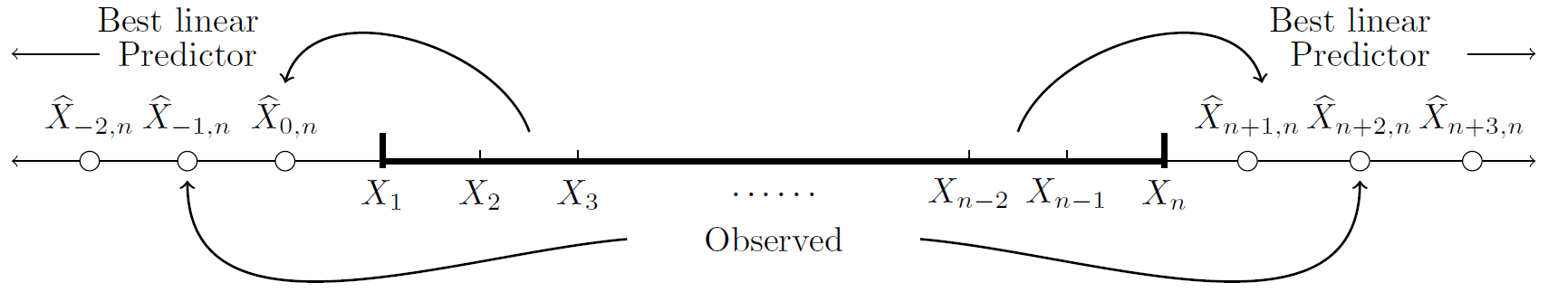
Figure 1: The complete DFT is the Fourier transform of $\{\widehat{X}_{\tau,n}\}$ over $\tau\in\mathbb{Z}$.

Substituting (2.1) into (1.2) rewrites the predictive DFT as

$$\widehat{J}_{n}(\omega;f)=n^{-1/2}\sum_{t=1}^{n}X_{t}\left[\sum_{\tau=-\infty}^{0}\phi_{t,n}(\tau;f)e^{i\tau\omega}+\sum_{\tau=n+1}^{\infty}\phi_{t,n}(\tau;f)e^{i\tau\omega}\right].$$

In the following sections we propose a method for estimating $\widehat{J}_{n}(\omega;f)$, thus the complete DFT and corresponding periodogram, based on the above representation.

However, we conclude this section by attempting to understand the “origin” of the DFT in the analysis of a stationary time series. We do this by connecting the complete DFT with the orthogonal increment process of the associated time series. Suppose that $Z(\omega)$ is the orthogonal increment process associated with the stationary (Gaussian) time series $\{X_{t}\}_{t\in\mathbb{Z}}$ and $f$ the corresponding spectral density. By using Theorem 4.9.1 in Brockwell and Davis (2006) we can show that

$$\mathbb{E}\left[X_{\tau}|X_{1},\ldots,X_{n}\right]=\frac{1}{2\pi}\int_{0}^{2\pi}e^{-i\omega\tau}\mathbb{E}[dZ(\omega)|X_{1},\ldots,X_{n}]=\frac{\sqrt{n}}{2\pi}\int_{0}^{2\pi}e^{-i\omega\tau}\widetilde{J}_{n}(\omega;f)d\omega\quad\forall\tau\in\mathbb{Z}.$$

Based on the above, heuristically, $\mathbb{E}[dZ(\omega)|X_{1},\ldots,X_{n}]=\sqrt{n}\widetilde{J}_{n}(\omega;f)d\omega$ and $\sqrt{n}\widetilde{J}_{n}(\omega;f)$ is the derivative of the orthogonal increment process conditioned on the observed time series. Under Assumption 2.1, below, it can be shown that $\mathrm{var}[\widehat{J}_{n}(\omega;f)]=O(n^{-1})$, whereas $\mathrm{var}[J_{n}(\omega)]=f_{n}=O(1)$. Based on this, since $\widetilde{J}_{n}(\omega;f)=J_{n}(\omega)+\widehat{J}_{n}(\omega;f)$, then $\sqrt{n}\widetilde{J}_{n}(\omega;f)\approx\sqrt{n}J_{n}(\omega)$. Thus the regular DFT, $\sqrt{n}J_{n}(\omega)$, can be viewed as an approximation of the derivative of the orthogonal increment process conditioned on the observed time series.

2.1 The AR$(p)$ model and an AR$(\infty)$ approximation

We recall that complete periodogram involves $\widehat{J}_{n}(\omega;f)$ which is a function of the unknown spectral density. Thus the complete periodogram cannot be directly evaluated. Instead, the prediction coefficients need to be estimated. For general spectral density functions, this will be impossible since for each $\tau$, $\{\phi_{t,n}(\tau;f)\}_{t=1}^{n}$ is an unwieldy function of the autocovariance function. However, for certain spectral density functions, it is possible. Below we consider a class of models where $\widehat{J}_{n}(\omega;f)$ has a relatively simple analytic form. We will use this as a basis of obtaining an approximation of $\widehat{J}_{n}(\omega;f)$.

Suppose that $f_{p}(\omega)=\sigma^{2}|1-\sum_{j=1}^{p}a_{j}e^{-ij\omega}|^{-2}$ is the spectral density of the time series $\{X_{t}\}_{t\in\mathbb{Z}}$ (it is a finite order autoregressive model AR$(p)$) and where the characteristic polynomial associated with $\{a_{j}\}_{j=1}^{p}$ has roots lying outside the unit circle. Clearly, we can represent the time series $\{X_{t}\}_{t\in\mathbb{Z}}$ as

$$X_{t}=\sum_{j=1}^{p}a_{j}X_{t-j}+\varepsilon_{t}\quad t\in\mathbb{Z}$$

where $\{\varepsilon_{t}\}_{t\in\mathbb{Z}}$ are uncorrelated random variables with $\mathbb{E}[\varepsilon_{t}]=0$ and $\mathrm{var}[\varepsilon_{t}]=\sigma^{2}$. For finite order AR$(p)$ processes with autoregressive coefficients $\{a_{j}\}_{j=1}^{p}$, the best linear predictor of $X_{0}$ and $X_{n+1}$ given $\{X_{t}\}_{t=1}^{n}$ are $\widehat{X}_{0,n}=\sum_{j=1}^{p}a_{j}X_{j}$ and $\widehat{X}_{n+1,n}=\sum_{j=1}^{p}a_{j}X_{n+1-j}$ respectively. In general, we can iteratively define the best linear predictors $\widehat{X}_{1-\tau,n}$ and $\widehat{X}_{n+\tau,n}$ to be

$$\widehat{X}_{1-\tau,n}=\sum_{j=1}^{p}a_{j}\widehat{X}_{1-\tau+j,n}\quad\text{and}\quad\widehat{X}_{n+\tau,n}=\sum_{j=1}^{p}a_{j}\widehat{X}_{n+\tau-j,n}\qquad\textrm{ for }\tau\geq 1,$$

where $\widehat{X}_{t,n}=X_{t}$ for $1\leq t\leq n$. Using these expansions, SY20 (equation (2.15)) show that if $p\leq n$, then

$$\widehat{J}_{n}(\omega;f_{p})=\frac{n^{-1/2}}{a_{p}(\omega)}\sum_{\ell=1}^{p}X_{\ell}\sum_{s=0}^{p-\ell}a_{\ell+s}e^{-is\omega}+e^{in\omega}\frac{n^{-1/2}}{\overline{a_{p}(\omega)}}\sum_{\ell=1}^{p}X_{n+1-\ell}\sum_{s=0}^{p-\ell}a_{\ell+s}e^{i(s+1)\omega},$$ (2.2)

where $a_{p}(\omega)=1-\sum_{j=1}^{p}a_{j}e^{-ij\omega}$. The above expression tells us that for finite order autoregressive models, estimation of the predictive DFT, $\widehat{J}_{n}(\omega;f_{p})$, only requires us to estimate $p$ autoregressive parameters.

However, for general second order stationary time series, such simple expressions are not possible. But (2.2) provides a clue to obtaining a near approximation, based on the AR$(\infty)$ representation that many stationary time series satisfy. It is well known that if the spectral density $f$ is bounded and strictly positive with $\sum_{r\in\mathbb{Z}}|c(r)|<\infty$, then it has an AR$(\infty)$ representation see Baxter (1962) (see also equation (2.3) in Kreiss et al. (2011))

$$X_{t}=\sum_{j=1}^{\infty}a_{j}X_{t-j}+\varepsilon_{t}\quad t\in\mathbb{Z}$$

where $\{\varepsilon_{t}\}_{t\in\mathbb{Z}}$ are uncorrelated random variables. Unlike finite order autoregressive models, $\widehat{J}_{n}(\omega;f)$ cannot be represented in terms of $\{a_{j}\}_{j=1}^{\infty}$, since it only involves the sum of the best finite predictors (not infinite predictors). Instead, we define an approximation based on (2.2), but using the AR$(\infty)$ representation

$$\widehat{J}_{\infty,n}(\omega;f) = \frac{n^{-1/2}}{a(\omega;f)}\sum_{\ell=1}^{n}X_{\ell}\sum_{s=0}^{\infty}a_{\ell+s}e^{-is\omega}+e^{in\omega}\frac{n^{-1/2}}{\overline{a(\omega;f)}}\sum_{\ell=1}^{n}X_{n+1-\ell}\sum_{s=0}^{\infty}a_{\ell+s}e^{i(s+1)\omega}$$ (2.3)

$$= \frac{b(\omega;f)}{\sqrt{n}}\sum_{\ell=1}^{n}X_{\ell}\sum_{s=0}^{\infty}a_{\ell+s}e^{-is\omega}+e^{in\omega}\frac{\overline{b(\omega;f)}}{\sqrt{n}}\sum_{\ell=1}^{n}X_{n+1-\ell}\sum_{s=0}^{\infty}a_{\ell+s}e^{i(s+1)\omega}$$

where $a(\omega;f)=1-\sum_{j=1}^{\infty}a_{j}e^{-ij\omega}$ and $b(\omega;f)=1+\sum_{j=0}^{\infty}b_{j}e^{-ij\omega}$ ($\{b_{j}\}$ are the corresponding the moving average coefficients in the MA$(\infty)$ representation of $\{X_{t}\}$). Though seemingly unwieldy, (2.3) has a simple interpretation. It corresponds to the Fourier transform of the best linear predictors of $X_{\tau}$ given the infinite future $\{X_{t}\}_{t=1}^{\infty}$ (if $\tau\leq 0$) and $X_{\tau}$ given in the infinite past $\{X_{t}\}_{t=-\infty}^{n}$ (if $\tau>n$), but are truncated to the observed terms $\{X_{t}\}_{t=1}^{n}$. Of course, this is not $\widehat{J}_{n}(\omega;f)$. However, we show that

$$I_{\infty,n}(\omega;f)=[J_{n}(\omega)+\widehat{J}_{\infty,n}(\omega;f)]\overline{J_{n}(\omega)}$$ (2.4)

is a close approximation of the complete periodogram, $I_{n}(\omega;f)$. To do so, we require the following assumptions.

2.2 Assumptions and preliminary results

The first set of assumptions is on the second order structure of the time series.

Assumption 2.1

$\{X_{t}\}_{t\in\mathbb{Z}}$ is a second order stationary time series, where

• The spectral density, $f$, is a bounded and strictly positive function.

• For some $K\geq 1$, the autocovariance function is such that $\sum_{r\in\mathbb{Z}}|r^{K}c(r)|<\infty$.

Assumption 2.1(ii) implies that the spectral density $f$ is $\lfloor K\rfloor$ times continuously differentiable where $\lfloor K\rfloor$ denotes the largest integer smaller than or equal to $K$. Conversely, Assumption 2.1(ii) is satisfied for all spectral densities with (i) $\lceil K\rceil+1$ times continuously differentiable if $K\notin\mathbb{N}$ (where $\lceil K\rceil$ denotes the smallest integer larger than or equal to $K$) or (ii) $K+1$ times differentiable and $f^{(K+1)}(\cdot)$ is $\alpha$-Hölder continuous for some $0<\alpha\leq 1$ and $K\in\mathbb{N}$. We mention that under Assumption 2.1, the corresponding AR$(\infty)$ and MA$(\infty)$ coefficients are such that $\sum_{j\in\mathbb{Z}}|j^{K}a_{j}|<\infty$ and $\sum_{j\in\mathbb{Z}}|j^{K}b_{j}|<\infty$ (see Lemma 2.1 in Kreiss et al. (2011).

The next set of assumptions are on the higher order cumulants structure of the time series.

Assumption 2.2

$\{X_{t}\}$ is an $2m$-order stationary time series such that $\mathbb{E}[|X_{t}|^{2m}]<\infty$ and $\mathrm{cum}(X_{t},X_{t+s_{1}},...,X_{t+s_{h-1}})=\mathrm{cum}(X_{0},X_{s_{1}},\ldots,X_{s_{h-1}})=\kappa_{h}(s_{1},...,s_{h-1})$ for all $t,s_{1},...s_{h-1}\in\mathbb{Z}$ with $h\leq 2m$. Further, the joint cumulant $\{\kappa_{h}(s_{1},...,s_{h-1})\}$ satisfies

$$\sum_{s_{1},\ldots,s_{h-1}}|\kappa_{h}(s_{1},\ldots,s_{h-1})|<\infty\quad\textrm{for}\quad 2\leq h\leq 2m.$$

Before studying the approximation error when replacing $I_{n}(\omega;f)$ with $I_{\infty,n}(\omega;f)$ we first obtain some preliminary results on the complete periodogram $I_{n}(\omega;f)$.

Properties of the complete periodogram and comparisons with the regular periodogram

The following (unsurprising) result concerns the order of contribution of the predictive DFT in the complete periodogram. Suppose Assumptions 2.1 (with $K\geq 1$) and 2.2 (for $m=2$) hold. Let $\widehat{J}_{n}(\omega;f)$ be defined as in (1.2). Then

$$\mathbb{E}[\widehat{J}_{n}(\omega;f)\overline{J_{n}(\omega)}]=O(n^{-1}),\quad\mathrm{var}[\widehat{J}_{n}(\omega;f)\overline{J_{n}(\omega)}]=O(n^{-2}).$$ (2.5)

The details of the proof of the above can be found in Appendix A.1.

There are two main differences between the complete periodogram and the regular periodogram. The first is that the complete periodogram can be complex, however the imaginary part is mean zero and the variance is of order $O(n^{-1})$. Thus without any loss of generality we can focus on the real part of the complete periodogram $\widetilde{J}_{n}(\omega;f)\overline{J_{n}(\omega)}$, denotes $\operatorname{Re}\widetilde{J}_{n}(\omega;f)\overline{J_{n}(\omega)}$. Second, unlike the regular periodogram, $\operatorname{Re}\widetilde{J}_{n}(\omega;f)\overline{J_{n}(\omega)}$, can be negative. Therefore if positivity is desired it makes sense to threshold $\operatorname{Re}\widetilde{J}_{n}(\omega;f)\overline{J_{n}(\omega)}$ to be non-zero. Thresholding $\operatorname{Re}\widetilde{J}_{n}(\omega;f)\overline{J_{n}(\omega)}$ to be non-zero induces a small bias. But we observe from the simulations in Section 4 that the bias is small (see the middle column in Figures 2$-$4 where the average of the thresholded true complete periodogram for various models is given).

In the simulations, we observe that the variance of the complete periodogram tends to be larger than the variance of the regular periodogram, especially at frequencies where the spectral density peaks. To understand why, we focus on the case that the time series is Gaussian. For the complete periodogram, it can be shown that

$$\mathrm{var}[I_{n}(\omega;f)]=\mathrm{var}[\widetilde{J}_{n}(\omega;f)]\cdot\mathrm{var}[J_{n}(\omega)]+O(n^{-2}).$$

By Cauchy-Schwarz inequality, we have for all $n$ that

$$\mathrm{var}[\widetilde{J}_{n}(\omega;f)]\cdot\mathrm{var}[J_{n}(\omega)]\geq|\mathrm{cov}[\widetilde{J}_{n}(\omega;f),J_{n}(\omega)]|^{2}=f(\omega)^{2}.$$

Thus the variance of the complete periodogram is such that $\mathrm{var}[I_{n}(\omega;f)]\geq f(\omega)^{2}$. By contrast the variance of the regular periodogram is $\mathrm{var}[I_{n}(\omega)]\approx f_{n}(\omega)^{2}<f(\omega)^{2}$. Nevertheless, despite an increase in variance of the periodogram, our simulations suggest that this may be outweighed by a substantial reduction in the bias of the complete periodogram (see Figures 2$-$4 and Table 1).

The complete periodogram and its AR$(\infty)$ approximation

Our aim is to estimate the predictive component in the complete periodogram; $\widehat{J}_{n}(\omega;f)\overline{J_{n}(\omega)}$. As a starting point, we use the above assumptions to bound the difference between $I_{n}(\omega;f)$ and $I_{\infty,n}(\omega;f)$.

Theorem 2.1

Suppose Assumption 2.1 and 2.2 (for $m=2$) hold. Let $I_{n}(\omega;f)=\widetilde{J}_{n}(\omega;f)\overline{J_{n}(\omega)}$ and $I_{\infty,n}(\omega;f)$ is defined as in (2.4). Then

$$I_{\infty,n}(\omega;f) = I_{n}(\omega;f)+\Delta_{0}(\omega),$$ (2.6)

where $\sup_{\omega}\mathbb{E}[\Delta_{0}(\omega)]=O\left(n^{-K}\right)$, $\sup_{\omega}\mathrm{var}[\Delta_{0}(\omega)]=O\left(n^{-2K}\right)$.

PROOF. See Appendix A.1. $\Box$

A few comments on the above approximation are in order. Observe that the approximation error between the complete periodogram and its infinite approximation is of order $O(n^{-K})$. For AR$(p)$ processes (where $p\leq n$) this term would not be there. For AR$(\infty)$ representations with coefficients that geometrically decay (e.g., an ARMA process), then $|I_{\infty,n}(\omega;f)-I_{n}(\omega;f)|=O_{p}(\rho^{n})$, for some $0\leq\rho<1$. On the other hand, if the AR$(\infty)$ representation has an algebraic decaying coefficients, $a_{j}\sim|j|^{-K-1-\delta}$ (for some $\delta>0$), then $|I_{\infty,n}(\omega;f)-I_{n}(\omega;f)|=O_{p}(n^{-K})$. In summary, nothing that $I_{n}(\omega;f)$ is an unbiased estimator of $f$, if $K>1$, then $I_{\infty,n}(\omega;f)$ has a smaller bias than the regular periodogram.

Now the aim is to estimate $\widehat{J}_{\infty,n}(\omega;f)$. There are various ways this can be done. In this paper, we approximate the underlying time series with an AR$(p)$ process and estimate the AR$(p)$ parameters. This approximation will incur two sources of errors. The first is approximating an AR$(\infty)$ process with a finite order AR$(p)$ model, the second is the estimation error when estimating the parameters in the AR$(p)$ model. In the following section, we obtain bounds for these errors.

Remark 2.1 (Alternative estimation methods)

As pointed out by a referee for SY20, if the underlying spectral density is highly complex with several peaks, fitting a finite order AR$(p)$ model may not be able to reduce the bias. An alternative method is to use the smooth periodogram to estimate the predictive DFT. That is to estimate the AR$(\infty)$ parameters and MA$(\infty)$ transfer function $b(\omega)$ in (2.3) using an estimate of the spectral density function. This can be done by first estimating the cepstral coefficients (Fourier coefficients of $\log f(\omega)$) using the method Wilson (1972). Then, by using the recursive algorithms obtained in Pourahmadi(1983, 1984, 2000) and Krampe et al. (2018) one can extract estimators of AR$(\infty)$ and MA$(\infty)$ parameters from the cepstral coefficients. It is possible that the probabilistic bounds for the estimates obtained in Krampe et al. (2018) can be used to obtain bounds for the resulting predictive DFT, but this remains an avenue for future research.

2.3 An approximation of the complete DFT

We return to the definition of the predictive DFT in (1.2), which is comprised of the best linear predictors outside the domain of observation. In time series, it is common to approximate the best linear predictors with the predictors based on a finite AR$(p)$ recursion (the so called plug-in estimators; see Bhansali (1996) and Kley et al. (2019)). This approximation corresponds to replacing $f$ in $\widehat{J}_{n}(\omega;f)$ with $f_{p}$, where $f_{p}$ is the spectral density corresponding to “best fitting” AR$(p)$ model based on $f$.

It is well known that the best fitting AR$(p)$ coefficients, given the covariances $\{c(r)\}$, are

$$\underline{a}_{p}=(a_{1,p},...,a_{p,p})^{\prime}=R_{p}^{-1}\underline{r}_{p},$$ (2.7)

where $R_{p}$ is the $p\times p$ Toeplitz variance matrix with $(R_{p})_{(s,t)}=c(s-t)$ and $\underline{r}_{p}=(c(1),\ldots,c(p))^{\prime}$. This leads to the AR$(p)$ spectral density approximation of $f$

$$f_{p}(\omega)=\sigma^{2}|a_{p}(\omega)|^{-2},\quad\text{where}\quad a_{p}(\omega)=1-\sum_{j=1}^{p}a_{j,p}e^{-ij\omega}.$$

The coefficients $\{a_{j,p}\}_{j=1}^{p}$ are used to construct the plug-in prediction estimators for $X_{\tau}$ ($\tau\leq 0$ or $\tau>n$). This in turn gives the approximation of the predictive DFT $\widehat{J}_{n}(\omega;f_{p})$ where the analytic form for $\widehat{J}_{n}(\omega;f_{p})$ is given in (2.2), with the coefficients $a_{j}$ replaced with $a_{j,p}$.

Using $\widetilde{J}_{n}(\omega;f_{p})=J_{n}(\omega)+\widehat{J}_{n}(\omega;f_{p})$ we define the following approximation of the complete periodogram

$$I_{n}(\omega;f_{p})=\widetilde{J}_{n}(\omega;f_{p})\overline{J_{n}(\omega)}.$$ (2.8)

We now obtain a bound for the approximation error, where we replace $I_{\infty,n}(\omega;f)$ with $I_{n}(\omega;f_{p})$.

Theorem 2.2

Suppose Assumption 2.1 holds with $K>1$. Let $I_{\infty,n}(\omega;f)$ and $I_{n}(\omega;f_{p})$, be defined as in (2.4) and (2.8) respectively. Then we have

$$I_{n}(\omega;f_{p}) = I_{\infty,n}(\omega;f)+\Delta_{1}(\omega),$$ (2.9)

where $\sup_{\omega}\mathbb{E}[\Delta_{1}(\omega)]=O\left((np^{K-1})^{-1}\right)$, $\sup_{\omega}\mathrm{var}[\Delta_{1}(\omega)]=O\left((np^{K-1})^{-2}\right)$.

PROOF. See Appendix A.1. $\Box$

Applying Theorems 2.1 and 2.2, we observe that $I_{n}(\omega;f_{p})$ has a smaller bias than the regular periodogram

$$\mathbb{E}[I_{n}(\omega;f_{p})]=f(\omega)+O\left(\frac{1}{np^{K-1}}\right).$$

In particular, the bias is substantially smaller than the usual $O(n^{-1})$ bias. Indeed, if the true underlying process has an AR$(p^{*})$ representation where $p^{*}<p$, then the bias is zero.

However, in reality, the true spectral density and best fitting AR$(p)$ approximation $f$ and $f_{p}$ respectively are unknown, and they need to be estimated from the observed data.

To estimate the best fitting AR$(p)$ model, we replace the autocovariances with the sample autocovariances to yield the Yule-Walker estimator of the best fitting AR$(p)$ parameters

$$\underline{\widehat{a}}_{p}=(\widehat{a}_{1,p},\ldots,\widehat{a}_{p,p})^{\prime}=\widehat{R}_{p,n}^{-1}~{}\underline{\widehat{r}}_{p,n},$$ (2.10)

where $\widehat{R}_{p,n}$ is the $p\times p$ sample covariance matrix with $(\widehat{R}_{p,n})_{(s,t)}=\widehat{c}_{n}(s-t)$ and $\underline{\widehat{r}}_{p,n}=(\widehat{c}_{n}(1),\ldots,\widehat{c}_{n}(p))^{\prime}$ where $\widehat{c}_{n}(k)=n^{-1}\sum_{t=1}^{n-|k|}X_{t}X_{t+k}$. We define the estimated AR$(p)$ spectral density

$$\widehat{f}_{p}(\omega)=|\widehat{a}_{p}(\omega)|^{-2}\quad\textrm{where}\quad\widehat{a}_{p}(\omega)=1-\sum_{j=1}^{p}\widehat{a}_{j,p}e^{-ij\omega}.$$

Observe that we have ignored including an estimate of the innovation variance in $\widehat{f}_{p}(\omega)$ as it plays no role in the definition of $\widehat{J}_{n}(\omega;f_{p})$. Using this we define the estimated complete DFT as $\widetilde{J}_{n}(\omega;\widehat{f}_{p})=J_{n}(\omega)+\widehat{J}_{n}(\omega;\widehat{f}_{p})$, where

$$\widehat{J}_{n}(\omega;\widehat{f}_{p})=\frac{n^{-1/2}}{\widehat{a}_{p}(\omega)}\sum_{\ell=1}^{p}X_{\ell}\sum_{s=0}^{p-\ell}\widehat{a}_{\ell+s,p}e^{-is\omega}+e^{in\omega}\frac{n^{-1/2}}{\overline{\widehat{a}_{p}(\omega)}}\sum_{\ell=1}^{p}X_{n+1-\ell}\sum_{s=0}^{p-\ell}\widehat{a}_{\ell+s,p}e^{i(s+1)\omega}$$ (2.11)

and corresponding estimated complete periodogram based on $\widehat{f}_{p}$ is

$$I_{n}(\omega;\widehat{f}_{p})=\widetilde{J}_{n}(\omega;\widehat{f}_{p})\overline{J_{n}(\omega)}.$$ (2.12)

We now show that with the estimated AR$(p)$ parameters the resulting estimated complete periodogram has a smaller bias (in the sense of Bartlett) than the regular periodogram.

Theorem 2.3

Suppose Assumptions 2.1(i) and 2.2 (where $m\geq 6$ and is multiple of two) hold. Let $I_{n}(\omega;f_{p})$ and $I_{n}(\omega;\widehat{f}_{p})$ be defined as in (2.8) and (2.12) respectively. Then we have the following decomposition

$$I_{n}(\omega;\widehat{f}_{p})=I_{n}(\omega;f_{p})+\Delta_{2}(\omega)+R_{n}(\omega)$$ (2.13)

where $\Delta_{2}(\omega)$ is the dominating error with

$$\sup_{\omega}\mathbb{E}[\Delta_{2}(\omega)]=O\left(\frac{p^{3}}{n^{2}}\right),\quad\sup_{\omega}\mathrm{var}[\Delta_{2}(\omega)]=O\left(\frac{p^{4}}{n^{2}}\right)$$

and $R_{n}(\omega)$ is such that $\sup_{\omega}|R_{n}(\omega)|=O_{p}\left((p^{2}/n)^{m/4}\right)$.

PROOF. See Appendix A.1. $\Box$

We now apply Theorems 2.1$-$2.3 to obtain a bound for the approximation error between the estimated complete periodogram $I_{n}(\omega;\widehat{f}_{p})$ and the complete periodogram.

Corollary 2.1

Suppose Assumptions 2.1 ($K>1$) and 2.2 (where $m\geq 6$ and is a multiple of two) hold. Let $I_{n}(\omega;f)=\widetilde{J}_{n}(\omega;f)\overline{J_{n}(\omega)}$ and $I_{n}(\omega;\widehat{f}_{p})$ be defined as in (2.12) respectively. Then we have

$$I_{n}(\omega;\widehat{f}_{p})=I_{n}(\omega;f)+\Delta(\omega)+O_{p}\left(\frac{p^{m/2}}{n^{m/4}}\right),$$

where $\Delta(\omega)=\Delta_{0}(\omega)+\Delta_{1}(\omega)+\Delta_{2}(\omega)$ (with $\Delta_{j}(\cdot)$ as defined in Theorems 2.1$-$2.3),

$\sup_{\omega}\mathbb{E}[\Delta(\omega)]=O((np^{K-1})^{-1}+p^{3}/n^{2})$ and $\sup_{\omega}\mathrm{var}[\Delta(\omega)]=O(p^{4}/n^{2})$.

PROOF. The result immediately follows from Theorems 2.1$-$2.3. $\Box$

To summarize, by predicting across the boundary using the estimated AR$(p)$ parameters heuristically we have reduced the “bias” of the periodogram. More precisely, if the probabilistic error $R_{n}(\omega)$ is such that $\frac{p^{m/2}}{n^{m/4}}<<\frac{p^{3}}{n^{2}}$. Then the “bias” as in the sense of Bartlett is

$$\mathbb{E}[I_{n}(\omega;\widehat{f}_{p})]=f(\omega)+O\left(\frac{1}{np^{K-1}}+\frac{p^{3}}{n^{2}}\right).$$

Consequently, for $K>1$, and $p$ chosen such that

$$p^{3}/n\rightarrow 0,\quad\text{as}\quad p,n\rightarrow\infty,$$ (2.14)

then the “bias” will be less than the $O(n^{-1})$ order. This can make a substantial difference when $n$ is small or the underlying spectral density has a large peak. Of course in practice the order $p$ needs to be selected. This is usually done using the AIC. In which case the above results need to be replaced with $\widehat{p}$, where $\widehat{p}$ is selected to minimize the AIC

$$\text{AIC}(p)=\log\widehat{\sigma}_{p,n}^{2}+\frac{2p}{n},$$

$\widehat{\sigma}_{p,n}^{2}=\frac{1}{n-K_{n}}\sum_{t=K_{n}}^{n}(X_{t}-\sum_{j=1}^{p}\widehat{a}_{j,p}X_{t-j})^{2}$, $K_{n}$ is such that $K_{n}^{2+\delta}\sim n$ for some $\delta>0$ and the order $p$ is chosen such that $\widehat{p}=\arg\min_{1\leq k\leq K_{n}}\text{AIC}(k)$. To show that the selected $\widehat{p}$ satisfies (2.14), we use the conditions in Ing and Wei (2005) who assume that the underlying time series is a linear, stationary time series with an AR$(\infty)$ that satisfies Assumption K.1$-$K.4 in Ing and Wei (2005). Under Assumption 2.1, and applying Baxter’s inequality, the AR$(\infty)$ coefficients satisfy

$$\sum_{j=1}^{\infty}|a_{j}-a_{j,p}|^{2}\leq\big{(}\sum_{j=1}^{\infty}|a_{j}-a_{j,p}|\big{)}^{2}\leq C\big{(}\sum_{j=p+1}^{\infty}|a_{j}|\big{)}^{2}=O\left(p^{-2K}\right).$$ (2.15)

Under these conditions, Ing and Wei (2005) obtain a bound for $\widehat{p}$. In particular, if the underlying time series has an exponential decaying AR coefficients, then $\widehat{p}=O_{p}(\log n)$ (see Example 1 in Ing and Wei (2005)) on the other hand if the rate of decay is polynomial order satisfying (2.15), then $\widehat{p}=O_{p}(n^{1/(1+2K)})$ (see Example 2 in Ing and Wei (2005)). Thus, for for both these cases we have $\widehat{p}^{3}/n\stackrel{{\scriptstyle P}}{{\rightarrow}}0$ and $\widehat{p}\stackrel{{\scriptstyle P}}{{\rightarrow}}\infty$ as $n\rightarrow\infty$.

In summary, using the AIC as a method for selecting $p$, yields an estimated complete periodogram that has a lower bias than the regular periodogram.

Remark 2.2 (Possible extensions)

There are two generalisations which are of interest. The first is whether these results generalize to the long memory time series setting. Our preliminary analysis suggests that it does. However, it is technically quite challenging to prove. The second is how to deal with missing observations in the observed time series. Imputation is a classical method for missing time series. Basic calculations suggest that imputation in the complete DFT, but setting the missing values to zero in the regular DFT, may yield a near unbiased complete periodogram. Again, we leave this for future research.

2.4 The tapered complete periodogram

We recall that the complete periodogram extends the “domain” of observation by predicting across the boundary for one of the DFTs, but keeping the other DFT the same. Our simulations suggest that a further improvement can be made by “softening” the boundary of the regular DFT by using a data taper. Unusually, unlike the classical data taper, we only taper the regular DFT, but keep the complete DFT as in (1.1). Precisely we define the tapered complete periodogram as

$$I_{\underline{h},n}(\omega;f)=\widetilde{J}_{n}(\omega;f)\overline{J_{\underline{h},n}(\omega)},\textrm{ where }J_{\underline{h},n}(\omega)=n^{-1/2}\sum_{t=1}^{n}h_{t,n}X_{t}e^{it\omega}$$

and $\underline{h}=\{h_{t,n}\}_{t=1}^{n}$ are positive weights. Again by using that $\mathrm{cov}[X_{t}.\widehat{X}_{\tau,n}]=c(t-\tau)$ for $1\leq t\leq n$ and $\tau\in\mathbb{Z}$ it is straightforward to show that

$$\mathbb{E}[I_{\underline{h},n}(\omega;f)]=\big{(}n^{-1}\sum_{t=1}^{n}h_{t,n}\big{)}\cdot f(\omega)\quad\textrm{for}\quad\omega\in[0,\pi].$$

Thus to ensure that $I_{\underline{h},n}(\omega;f)$ is an unbiased estimator of $f$, we constrain the tapered weights to be such that $\sum_{t=1}^{n}h_{t,n}=n$. Unlike the regular tapered periodogram, for any choice of $\{h_{t,n}\}$ (under the constraint $\sum_{t=1}^{n}h_{t,n}=n$), $I_{\underline{h},n}(\omega;f)$ will be an unbiased estimator of (no smoothness assumptions on the taper is required). But it seems reasonable to use standard tapers when defining $\{h_{t,n}\}$. In particular, to let

$$h_{t,n}=c_{n}h_{n}(t/n)$$

where $c_{n}=n/H_{1,n}$ and

$$H_{q,n}=\sum_{t=1}^{n}h_{n}(t/n)^{q},\qquad q\geq 1.$$ (2.16)

A commonly used taper is the Tukey (also called the cosine-bell) taper, where

$$h_{n}\left(\frac{t}{n}\right)=\left\{\begin{array}[]{ll}\frac{1}{2}[1-\cos(\pi(t-\frac{1}{2})/d)]&1\leq t\leq d\\ 1&d+1\leq t\leq n-d\\ \frac{1}{2}[1-\cos(\pi(n-t+\frac{1}{2})/d)]&n-d+1\leq t\leq n\end{array}.\right.$$ (2.20)

Since we do not observe the spectral density $f$, we use the estimated tapered complete periodogram

$$I_{\underline{h},n}(\omega;\widehat{f}_{p})=\widetilde{J}_{n}(\omega;\widehat{f}_{p})\overline{J_{\underline{h},n}(\omega)}$$ (2.21)

where $\widehat{f}_{p}$ is defined in Section 2.3. In the corollary below we obtain that the asymptotic bias of the estimated tapered complete periodogram, this result is analogous to the non-tapered result in Corollary 2.1.

Corollary 2.2

Suppose the Assumptions in Corollary 2.1 hold. Let $I_{\underline{h},n}(\omega;\widehat{f}_{p})$ be defined as in (2.21) where $\sum_{t=1}^{n}h_{t,n}=n$ and $\sup_{t,n}|h_{t,n}|<\infty$. Then we have

$$I_{\underline{h},n}(\omega;\widehat{f}_{p})=I_{\underline{h},n}(\omega;f)+\Delta_{\underline{h}}(\omega)+O_{p}\left(\frac{p^{m/2}}{n^{m/4}}\right),$$

where $\sup_{\omega}\mathbb{E}[\Delta_{\underline{h}}(\omega)]=O\left((np^{K-1})^{-1}+p^{3}/n^{2}\right)$ and $\sup_{\omega}\mathrm{var}[\Delta_{\underline{h}}(\omega)]=O\left(p^{4}/n^{2}\right)$.

PROOF. See Appendix A.2. $\Box$

Theoretically, it is unclear using the tapered estimated complete improves on the non-tapered estimated complete periodogram. But in the simulations, we do observe an improvement in the bias of the estimator when using (2.20) with $d=n/10$ (this will require further research). In contrast, in Section 3 we show that the choice of data taper does have an impact on the variance of estimators based on the complete periodogram.

3 The integrated complete periodogram

We now apply the estimated (tapered) complete periodogram to estimating parameters in a time series. Many parameters in time series can be rewritten in terms of the integrated spectral mean

$$A(g)=\frac{1}{2\pi}\int_{0}^{2\pi}g(\omega)f(\omega)d\omega,$$

where $g(\cdot)$ is an integrable function that is determined by an underlying parameter, $A(g)$. Examples of interesting functions $g$ are discussed at the end of this section.

The above representation motivates the following estimator of $A(g)$, where we replace the spectral density function $f$ with the regular periodogram, to yield the following estimators

$$A_{I,n}(g)=\frac{1}{2\pi}\int_{0}^{2\pi}g(\omega)I_{n}(\omega)d\omega\quad\textrm{or}\quad A_{S,n}(g)=\frac{1}{n}\sum_{k=1}^{n}g(\omega_{k,n})I_{n}(\omega_{k,n}),$$ (3.1)

of $A(g)$ where $\omega_{k,n}=\frac{2\pi k}{n}$. See, for example, Milhøj (1981); Dahlhaus and Janas (1996); Bardet et al. (2008); Eichler (2008); Niebuhr and Kreiss (2014); Mikosch and Zhao (2015) and Subba Rao (2018). However, similar to the regular periodogram, the integrated regular periodogram has an $O(n^{-1})$ bias

$$\mathbb{E}[A_{x,n}(g)]=A(g)+O(n^{-1})\quad x\in\{I,S\}$$

which can be severe for “peaky” spectral density functions and small sample sizes. The bias in the case that an appropriate tapered periodogram is used instead of the regular periodogram will be considerably smaller and of order $O(n^{-2})$. Ideally, we could replace the periodogram in (3.1) with the complete periodogram $I_{n}(\omega;f)$ this would produce an unbiased estimator. Of course, this is infeasible, since $f$ is unknown. Thus motivated by the results in Section 2.3, to reduce the bias in $A_{x,n}(g)$ we propose replacing $I_{n}(\omega)$ with the estimated complete periodogram $I_{n}(\omega;\widehat{f}_{p})$ or the tapered complete periodogram $I_{\underline{h},n}(\omega;\widehat{f}_{p})$ to yield the estimated integrated complete periodogram

$$A_{I,n}(g;\widehat{f}_{p})=\int_{0}^{2\pi}g(\omega)I_{\underline{h},n}(\omega;\widehat{f}_{p})d\omega\quad\textrm{and}\quad A_{S,n}(g;\widehat{f}_{p})=\frac{1}{n}\sum_{k=1}^{n}g(\omega_{k,n})I_{\underline{h},n}(\omega_{k,n};\widehat{f}_{p})$$ (3.2)

of $A(g)$. Note that the above formulation allows for the non-tapered complete periodogram (by setting $h_{t,n}=1$ for $1\leq t\leq n$).

In the following theorem, we show that the (estimated) integrated complete periodogram has a bias that has lower order than the integrated regular periodogram and is asymptotically “closer” to the ideal integrated complete periodogram $A_{x,n}(g;f)$ than the integrated regular periodogram.

Theorem 3.1

Suppose the assumptions in Corollary 2.1 hold. Further, suppose that the functions $g$ and its derivative are continuous on the torus $[0,2\pi]$. For $x\in\{I,S\}$, define $A_{x,n}(g;f)$ and $A_{x,n}(g;\widehat{f}_{p})$ as in (3.1) and (3.2) respectively, where $\sum_{t=1}^{n}h_{t,n}=n$ and

$\sup_{t,n}|h_{t,n}|<\infty$. Then

$$A_{x,n}(g;\widehat{f}_{p})=A_{x,n}(g;f)+\Delta(g)+O_{p}\left(\frac{p^{m/2}}{n^{m/4}}\right)$$

where $\mathbb{E}[\Delta(g)]=O\left((np^{K-1})^{-1}+p^{3}/n^{2}\right)$ and $\mathrm{var}[\Delta(g)]=O\left((np^{K-1})^{-2}+p^{6}/n^{3}\right)$.

PROOF. See Appendix A.2. $\Box$

From the above theorem we observe that if $m\geq 6$, then the term $\Delta(g)=O_{p}((np^{K-1})^{-1}+p^{3}/n^{3/2})$ dominates the probablistic error. This gives

$$A_{x,n}(g;\widehat{f}_{p})=A_{x,n}(g;f)+O_{p}\left(\frac{1}{np^{K-1}}+\frac{p^{3}}{n^{3/2}}\right).$$

Further, in the case of the integrated complete periodogram if $\frac{p^{m/2}}{n^{m/4}}<<\frac{p^{3}}{n^{2}}$, then the bias (in the sense of Bartlett) is

$$\mathbb{E}[A_{I,n}(g;\widehat{f}_{p})]=A(g)+O\left(\frac{1}{np^{K-1}}+\frac{p^{3}}{n^{2}}\right).$$

since $\mathbb{E}[A_{I,n}(g;f)]=A(g)$.

We now evaluate an expression for the asymptotic variance of $A_{x,n}(g;\widehat{f}_{p})$. We show that asymptotically the variance is same as if the predictive part of the periodogram; $\widehat{J}_{n}(\omega;\widehat{f}_{p})\overline{J_{\underline{h},n}(\omega)}$ were not included in the definition of $I_{\underline{h},n}(\omega;\widehat{f}_{p})$. To do so, we require the condition

$$\frac{H_{1,n}}{H_{2,n}^{1/2}}\left(\frac{p^{3}}{n^{3/2}}\right)\rightarrow 0\quad\text{as}\quad p,n\rightarrow\infty,$$ (3.3)

which ensures the predictive term is negligible as compared to the main term. Observe that, by using the Cauchy-Schwarz inequality, (3.3) holds for all tapers if $p^{3}/n\rightarrow 0$ as $p,n\rightarrow\infty$. Therefore, by the same argument at the end of Section 2.3, if the order $p$ is selected using the AIC, (3.3) holds for any taper.

Corollary 3.1

Suppose the assumptions in Corollary 2.1 hold. Let the data taper $\{h_{t,n}\}$ be such that $h_{t,n}=c_{n}h_{n}(t/n)$ where $c_{n}=n/H_{1,n}$ and $h_{n}:[0,1]\rightarrow\mathbb{R}$ is a sequence of taper functions which satisfy the taper conditions in Section 5, Dahlhaus (1988). For $x\in\{I,S\}$, define $A_{x,n}(g;\widehat{f}_{p})$ as in (3.2) and suppose $p,n$ satisfy (3.3). Then

$$\frac{H_{1,n}^{2}}{H_{2,n}}\mathrm{var}[A_{x,n}(g;\widehat{f}_{p})]=\left(V_{1}+V_{2}+V_{3}\right)+o(1)$$

where $H_{q,n}$ is defined in (2.16),

$$V_{1} = \frac{1}{2\pi}\int_{0}^{2\pi}g(\omega)\overline{g(-\omega)}f(\omega)^{2}d\omega,\quad V_{2}=\frac{1}{2\pi}\int_{0}^{2\pi}|g(\omega)|^{2}f(\omega)^{2}d\omega\quad\textrm{and}$$

$$V_{3} = \frac{1}{(2\pi)^{2}}\int_{0}^{2\pi}\int_{0}^{2\pi}g(\omega_{1})\overline{g(\omega_{2})}f_{4}(\omega_{1},-\omega_{1},\omega_{2})d\omega_{1}d\omega_{2},$$

where $f_{4}$ is the $4$th order cumulant spectrum.

PROOF. See Appendix A.2. $\Box$

From the above, we observe that when tapering is used, the asymptotic variance of $A_{x,n}(g;\widehat{f}_{p})$ is $O(H_{2,n}/H_{1,n}^{2})$. If $h_{n}\equiv h$ for all $n$ for some $h:[0,1]\rightarrow\mathbb{R}$ with bounded variation, then above rate has the limit

$$\frac{nH_{2,n}}{H_{1,n}^{2}}\rightarrow\frac{\int_{0}^{1}h(x)^{2}dx}{\left(\int_{0}^{1}h(x)dx\right)^{2}}\geq 1.$$

In general, to understand how it compares to the case where no tapering is used, we note that by the Cauchy-Schwarz inequality $H_{2,n}/H_{1,n}^{2}\geq n^{-1}$, where we attain equality $H_{2,n}/H_{1,n}^{2}=n^{-1}$ if and only if no tapering is used. Thus, typically the integrated tapered complete periodogram will be less efficient than the integrated (non-tapered) complete periodogram. However if $nH_{2,n}/H_{1,n}^{2}\rightarrow 1$ as $n\rightarrow\infty$, then using the tapered complete periodogram in the estimator leads to an estimator that is asymptotically as efficient as the tapered complete periodogram (and regular periodogram).

Remark 3.1 (Distributional properties of $A_{x,n}(g;\widehat{f}_{p})$)

By using Theorems 3.1 and Corollary 3.1 $A_{x,n}(g;\widehat{f}_{p}),$ $A_{x,n}(g;f)$ and $A_{x,\underline{h}}(g)$ (where $A_{x,\underline{h}}(g)$ is defined as in (3.1) but with $I_{\underline{h},n}(\omega)$ replacing $I_{n}(\omega)$) share the same asymptotic distributional properties. In particular, if (3.3) holds, then the asymptotic distributions $A_{x,n}(g;\widehat{f}_{p})$ and $A_{x,\underline{h}}(g)$ are equivalent. Thus if asymptotic normality of $A_{x,\underline{h}}(g)$ can be shown, then $A_{x,n}(g;\widehat{f}_{p})$ is also asymptotically normal with the same limiting variance (given in Corollary 3.1).

Below we apply the integrated complete periodogram to estimating various parameters.

Example: Autocovariance estimation

By Bochner’s theorem, the autocovariance function at lag $r$, $c(r)$, can be represented as

$$c(r)=A\left(\cos(r\cdot)\right)=\frac{1}{2\pi}\int_{0}^{2\pi}\cos(r\omega)f(\omega)d\omega.$$

In order to estimate $\{c(r)\}$, we replace $f$ with the integrated complete periodogram to yield the estimator

$$\widehat{c}_{n}(r;\widehat{f}_{p})=A_{I,n}(\cos(r\cdot);\widehat{f}_{p})\ =\frac{1}{2\pi}\int_{0}^{2\pi}\cos(r\omega)I_{\underline{h},n}(\omega;\widehat{f}_{p})d\omega.$$

$I_{\underline{h},n}(\omega;\widehat{f}_{p})$ can be negative, in such situations, the sample autocovariance is not necessarily positive definite. To ensure a positive definiteness, we threshold the complete periodogram to be greater than a small cutoff value $\delta>0$. This results in a sample autocovariance $\{\widehat{c}_{T,n}(r;\widehat{f}_{p})\}$ which is guaranteed to be positive definite, where

$$\widehat{c}_{T,n}(r;\widehat{f}_{p})=\frac{1}{2\pi}\int_{0}^{2\pi}\cos(r\omega)\max\{I_{\underline{h},n}(\omega;\widehat{f}_{p}),\delta\}d\omega.$$

This method is illustrated with simulations in Appendix B.1.

Example: Spectral density estimation

Typically, to estimate the spectral density one “smooths” the periodogram using the spectral window function. The same method can be applied to the complete periodogram. Let $W$ be a non-negative symmetric function where $\int W(u)du=2\pi$ and $\int W(u)^{2}du<\infty$. Define $W_{h}(\cdot)=(1/h)W(\cdot/h)$, where $h$ is a bandwidth. A review of different spectral windows and their properties can be found in Priestley (1981) and Section 10.4 of Brockwell and Davis (2006) and references therein. For $\lambda\in[0,\pi]$, we choose $g(\omega)=g_{\lambda}(\omega)=W_{h}(\lambda-\omega)$. Then the (estimated) integrated complete periodogram of the spectral density $f$ is

$$\widehat{f}_{n}(\lambda;\widehat{f}_{p})=A_{I,n}(g_{\lambda};\widehat{f}_{p})=\frac{1}{2\pi}\int_{0}^{2\pi}W_{h}(\lambda-\omega)I_{\underline{h},n}(\omega;\widehat{f}_{p})d\omega.$$

The method is illustrated with simulations in Section 4.2.

Example: Whittle likelihood

Suppose that $\mathcal{F}=\{f_{\theta}(\cdot):\theta\in\Theta\}$ for some compact $\Theta\in\mathbb{R}^{d}$ is a parametric family of spectral density functions. The celebrated Whittle likelihood, Whittle (1951, 1953) is a measure of “distance” between the periodogram and the spectral density. The parameter which minimises the (negative log) Whittle likelihood is used as an estimator of the spectral density. Replacing the periodogram with the complete periodogram we define a variant of the Whittle likelihood as

$$K_{n}(\theta) = \frac{1}{2\pi}\int_{0}^{2\pi}\left(\frac{I_{\underline{h},n}(\omega;\widehat{f}_{p})}{f_{\theta}(\omega)}+\log f_{\theta}(\omega)\right)d\omega$$

$$= A_{I,n}(f_{\theta}^{-1};\widehat{f}_{p})+\frac{1}{2\pi}\int_{0}^{2\pi}\log f_{\theta}(\omega)d\omega.$$

In SY20 we showed that using the non-tapered DFT $A_{S,n}(f_{\theta}^{-1};f_{\theta})=\underline{X}_{n}^{\prime}\Gamma_{\theta}^{-1}\underline{X}_{n}$ where $\underline{X}_{n}^{\prime}=(X_{1},\ldots,X_{n})$ and $\Gamma_{\theta}$ is the Toeplitz matrix corresponding to the spectral density $f_{\theta}$. $K_{n}(\theta)$ is a variant of the frequency domain quasi-likelihoods described in SY20. We mention that there aren’t any general theoretical guarantees that the bias corresponding to estimators based on $K_{n}(\theta)$ is lower than the bias of the Whittle likelihood (though simulations suggest this is usually the case). Expression for the asymptotic bias of $K_{n}(\theta)$ are given in SY20, Appendix E.

4 Simulations

To understand the utility of the proposed methods, we now present some simulations. For reasons of space, we focus on the Gaussian time series (noting that the methods also apply to non-Gaussian time series). In the simulations we use the following AR$(2)$ and ARMA$(3,2)$ models (we let $B$ denote the backshift operator)

• $\phi(B)X_{t}=\varepsilon_{t}$ with $\phi(z)=(1-\lambda e^{\frac{\pi}{2}i}z)(1-\lambda e^{-\frac{\pi}{2}i}z)$ for $\lambda\in\{0.7,0.9,0.95\}$.

• $\phi(B)X_{t}=\psi(B)\varepsilon_{t}$ with $\left\{\begin{array}[]{l}\phi(z)=(1-0.7z)(1-0.9e^{i}z)(1-0.9e^{-i}z)\\ \psi(z)=1+0.5z+0.5z^{2}\end{array}\right.$.

where $\mathbb{E}[\varepsilon_{t}]=0$ and $\mathrm{var}[\varepsilon_{t}]=1$. We observe that the peak of the spectral density for the AR$(2)$ model (M1) becomes more pronounced as $\lambda$ approaches one (at frequency $\pi/2$). The ARMA$(3,2)$ model (M2) has peaks at zero and $\pi/2$, further, it clearly does not have a finite order autoregressive representation.

We consider three different sample sizes: $n=$ 20 (extremely small), 50 (small), and 300 (large) to understand how the proposed methods perform over different sample sizes. All simulations are conducted at over $B=5,000$ replications.

Our focus will be on accessing the validity of our method in terms of bias, standard deviation, and mean squared error. We will compare (a) various periodograms and (b) the spectral density estimators based on smoothing the various periodograms. Simulations where we compare estimators of the autocorrelation function based on the various periodograms can be found in Appendix B.1. The periodograms we will consider are (i) the regular periodogram (ii) the tapered periodogram $I_{\underline{h},n}(\omega)$, where

$$I_{\underline{h},n}(\omega)=\big{|}H_{2,n}^{-1/2}\sum_{t=1}^{n}h_{n}\left(t/n\right)X_{t}e^{it\omega}\big{|}^{2},$$

$H_{2,n}$ is defined in (2.16), (iii) the estimated complete periodogram (2.12) and (iv) the tapered complete periodogram (2.21). To understand the impact estimation has on the complete periodogram, for a model (M1) we also evaluate the complete periodogram using the true AR$(2)$ parameters, as this is an AR$(2)$ model the complete periodogram has an analytic form in terms of the AR parameters. This allows us to compare the infeasible complete periodogram $I_{n}(\omega;f)$ with the feasible estimated complete periodogram $I_{n}(\omega,\widehat{f}_{p})$.

For the tapered periodogram and tapered complete periodogram, we use the Tukey taper defined in (2.20). Following Tukey’s rule of thumb, we set the level of tapering to $10\%$ (which corresponds to $d=n/10$). When evaluating the estimated complete and tapered complete periodogram, we select the order $p$ using the AIC, and we estimate the AR coefficients using the Yule-Walker estimator.

Processing the complete and tapered complete periodogram For both the complete and tapered complete periodogram, it is possible to have an estimator that is complex and/or the real part is negative. In the simulations, we found that a negative $\operatorname{Re}I_{n}(\omega_{k,n};\widehat{f}_{p})$ tends to happen more for the spectral densities with large peaks and the true spectral density is close to zero. To avoid such issues, for each frequency, we take the real part of the estimator and thresholding with a small positive value. In practice, we take the threshold value $\delta=10^{-3}$. Thresholding induces a small bias in the estimator, but, at least in our models, the effect is negligible (see the middle column in Figures 2$-$4).

4.1 Comparing the different periodograms

In this section, we compare the bias and variance of the various periodograms for models (M1) and (M2).

Figures 2$-$4 give the average (left panels), bias (middle panels), and standard deviation (right panels) of the various periodograms for the different models and samples sizes. The dashed line in each panel is the true spectral density. It is well known that $\mathrm{var}[I_{n}(\omega)]\approx f(\omega)^{2}$ for $0<\omega<\pi$ and $\mathrm{var}[I_{n}(\omega)]\approx 2f(\omega)^{2}$ for $\omega=0,\pi$. Therefore, for a fair comparision in the standard deviation plot for the true spectral density we replace $\sqrt{2}f(0)$ and $\sqrt{2}f(\pi)$ with $f(0)$ and $f(\pi)$ respectively.

In Figures 2$-$4 (left and middle panels), we observe that in general, the various complete periodograms give a smaller bias than the regular periodogram and the tapered periodogram. This corroborates our theoretical findings that that complete periodogram smaller bias than the $O(n^{-1})$ rate. As expected, we observe that the true (based on the true AR parameters) complete periodogram (red) has a smaller bias than the estimated complete (orange) and tapered complete periodograms (green). Such an improvement is most pronounced near the peak of the spectral density and it is most clear when the sample size $n$ is small. For example, in Figure 2, when the sample size is extremely small ($n$=20), the bias of the various complete periodograms reduce by more than a half the bias of the regular and tapered periodogram. As expected, the true complete periodogram (red) for (M1) has very little bias even for the sample size $n=20$. The slight bias that is observed is due to thresholding the true complete periodogram to be positive (which as we mentioned above induces a small, additional bias). We also observe that for the same sample size that the regular tapered periodogram (blue) gives a slight improvement in the bias over the regular periodogram (black), but it is not as noticeable as the improvements seen when using the complete periodograms. It is interesting to observe that even for model (M2), which does not have a finite autoregressive representation (thus the estimated complete periodogram incurs additional errors) also has a considerable improvement in bias.

As compared with the regular periodogram, the estimated complete periodogram incurs two additional sources of errors. In Section 2.2 we showed that the variance of the true complete periodogram tends to be larger than the variance of the regular periodogram. Further in Theorem 2.3 we showed that using the estimated Yule-Walker estimators in the predictive DFT leads to an additional $O(p^{4}/n^{2})$ variance in the estimated complete periodogram. This means for small sample sizes and large $p$ the variance can be quite large. We observe both these effects in the right panels in Figures 2$-$4. In particular, the standard deviation of the various complete periodograms tends to be greater than the asymptotic standard deviation $f(\omega)$ close to the peaks. On the other hand, the standard deviation of the regular periodogram tends to be smaller than $f(\omega)$.

In order to globally access bias/variance trade-off for the different periodograms, we evaluate their mean squared errors. We consider two widely used metrics (see, for example, Hurvich (1988)). The first is the integrated relative mean squared error

$$\text{IMSE}=\frac{1}{nB}\sum_{k=1}^{n}\sum_{j=1}^{B}\left(\frac{\widetilde{I}^{(j)}(\omega_{k,n})}{f(\omega_{k,n})}-1\right)^{2}$$ (4.1)

where $\widetilde{I}^{(j)}(\cdot)$ is the $j$th replication of one of the periodograms. The second metric is the integrated relative bias

$$\text{IBIAS}=\frac{1}{n}\sum_{k=1}^{n}\left(\frac{B^{-1}\sum_{j=1}^{B}\widetilde{I}^{(j)}(\omega_{k,n})}{f(\omega_{k,n})}-1\right)^{2}.$$ (4.2)

Table 1 summarizes the IMSE and IBIAS of each periodogram over the different models and sample sizes. In most cases, the tapered periodogram, true complete periodogram (when it can be evaluated) and the two estimated complete periodograms have a smaller IMSE and IBIAS than the regular periodogram. As expected, the IBIAS of the (true) complete periodogram is almost zero (rounded off to three decimal digits) for (M1). The estimated complete and tapered complete periodogram has significantly small IBIAS than the regular and tapered periodogram. But interestingly, when the spectral density is “more peaky” the estimated complete periodograms tend to have a smaller IMSE than the regular and tapered periodogram. Suggesting that for peaky spectral densities, the improvement in bias outweighs the increase in the variance. Comparing the tapered complete periodogram with the non-tapered complete periodogram we observe that the tapered complete periodogram tends to have a smaller IBIAS (and IMSE) than the non-tapered (estimated) complete periodogram.

The above results suggest that the proposed periodograms can considerably reduce the small sample bias without increasing the variance by too much.

Figure 2: The average (left), bias (middle), and standard deviation (right) of the spectral density (black dashed) and the five different periodograms for Models (M1) and (M2). Length of the time series $n=20$.

Figure 3: Periodogram: Same as Figure 2 but for $n=50$.

Figure 4: Periodogram: Same as Figure 2 but for $n=300$.

Model	$n$	metric	Regular	Tapered	Complete(True)	Complete(Est)	Tapered complete
(M1), $\lambda=0.7$	20	IMSE	$1.284$	$1.262$	$1.127$	$1.323$	$1.325$
		IBIAS	$0.011$	$0.009$	$0$	$0.002$	$0.001$
	50	IMSE	$1.101$	$1.069$	$1.055$	$1.098$	$1.117$
		IBIAS	$0.002$	$0.001$	$0$	$0$	$0$
	300	IMSE	$1.014$	$1.006$	$1.007$	$1.009$	$1.046$
		IBIAS	$0$	$0$	$0$	$0$	$0$
(M1), $\lambda=0.9$	20	IMSE	$2.184$	$2.155$	$1.226$	$1.466$	$1.447$
		IBIAS	$0.152$	$0.159$	$0$	$0.009$	$0.007$
	50	IMSE	$1.434$	$1.217$	$1.112$	$1.166$	$1.145$
		IBIAS	$0.029$	$0.011$	$0$	$0.001$	$0$
	300	IMSE	$1.059$	$1.010$	$1.017$	$1.020$	$1.047$
		IBIAS	$0.001$	$0$	$0$	$0$	$0$
(M1), $\lambda=0.95$	20	IMSE	$3.120$	$4.102$	$1.298$	$1.527$	$1.560$
		IBIAS	$0.368$	$0.664$	$0$	$0.022$	$0.018$
	50	IMSE	$2.238$	$1.486$	$1.211$	$1.295$	$1.200$
		IBIAS	$0.151$	$0.045$	$0$	$0.002$	$0.001$
	300	IMSE	$1.133$	$1.017$	$1.033$	$1.037$	$1.049$
		IBIAS	$0.004$	$0$	$0$	$0$	$0$
(M2)	20	IMSE	$457.717$	$136.830$	$-$	$26.998$	$4.836$
		IBIAS	$157.749$	$58.717$	$-$	$4.660$	$0.421$
	50	IMSE	$81.822$	$3.368$	$-$	$3.853$	$1.357$
		IBIAS	$26.701$	$0.692$	$-$	$0.288$	$0.002$
	300	IMSE	$4.376$	$1.015$	$-$	$1.274$	$1.049$
		IBIAS	$0.787$	$0$	$-$	$0.003$	$0$

Table 1: IMSE and IBIAS for the different periodograms and models.

4.2 Spectral density estimation

Finally, we estimate the spectral density function by smoothing the periodogram. We consider the smoothed periodogram of the form

$$\breve{f}(\omega_{k,n})=\sum_{|j|\leq m}W(j)\widetilde{I}_{n}(\omega_{j+k,n})$$

where $\widetilde{I}_{n}(\cdot)$ is one of the candidate periodograms described in the previous section and $\{W(\cdot)\}$ are the positive symmetric weights satisfy the conditions (i) $\sum_{|j|\leq m}W(j)=1$ and (ii) $\sum_{|j|\leq m}W^{2}(j)\rightarrow 0$. The bandwidth $m=m(n)$ satisfies the condition $m/n\rightarrow 0$ as $m,n\rightarrow\infty$. We use the following three spectral window functions:

• (The Daniell Window) $\widetilde{W}(j)=\frac{1}{2m+1}$, $|j|\leq m$.

• (The Bartlett Window) $\widetilde{W}(j)=1-\frac{|j|}{m}$, $|j|\leq m$.

• (The Hann Window) $\widetilde{W}(j)=\frac{1}{2}[1-\cos(\frac{\pi(j+m)}{m})]$, $|j|\leq m$.

and normalize using $W(j)=\widetilde{W}(j)/\sum_{|j|\leq m}\widetilde{W}(j)$.

In this section, we only focus on estimating the spectral density of model (M2). We smooth the various periodogram using the three window functions described above. For each simulation, we calculate the IMSE and IBIAS (analogous to (4.1) and (4.2)). The bandwidth selection is also very important. One can extend the cross-validation developed for smoothing the regular periodogram (see Hurvich (1985), Beltrão and Bloomfield (1987) and Ombao et al. (2001)) to the complete periodogram and this may be an avenue of future research. In this paper, we simply use the bandwidth $m\approx n^{1/5}$ (in terms of order this corresponds to the optimal MSE).

The results are summarized in Table 2. We observe that smoothing with the tapered periodogram and the two different complete periodograms have a smaller IMSE and IBIAS as compared to the smooth regular periodogram. This is uniformly true for all the models, sample sizes, and window functions. When the sample size is small ($n=20$ and $50$), the smooth complete and tapered complete periodogram has a uniformly smaller IMSE and IBIAS than the smooth tapered periodogram for all window functions. For the large sample size ($n=300$), smoothing with the tapered periodogram and tapered complete periodogram gave similar results, whereas smoothing using the complete periodogram gives a slightly worse bias and MSE.

It is intriguing to note that the smooth complete tapered periodogram gives one the smallest IBIAS and IMSE as compared with all the other methods. These results suggest that spectral smoothing using the tapered complete periodogram may be very useful for studying the spectral density of short time series. Such data sets can arise in many situations, which as the analyses of nonstationary time series, where the local periodograms are often used.

$n$	$m$	Window	Metric	Regular	Tapered	Complete	Tapered complete
20	No smoothing		IMSE	$457.717$	$136.830$	$26.998$	$4.836$
			IBIAS	$157.749$	$58.717$	$4.660$	$0.421$
	2	Daniell	IMSE	$1775.789$	$1399.366$	$1008.590$	$943.855$
			IBIAS	$882.576$	$780.363$	$444.727$	$408.325$
		Bartlett	IMSE	$538.477$	$203.217$	$43.347$	$17.489$
			IBIAS	$203.010$	$100.178$	$13.270$	$6.391$
		Hann	IMSE	$538.477$	$203.217$	$43.347$	$17.489$
			IBIAS	$203.010$	$100.178$	$13.270$	$6.391$
50	No smoothing		IMSE	$81.822$	$3.368$	$3.853$	$1.357$
			IBIAS	$26.701$	$0.692$	$0.288$	$0.002$
	2	Daniell	IMSE	$87.485$	$7.227$	$5.138$	$3.308$
			IBIAS	$33.327$	$3.947$	$1.954$	$1.346$
		Bartlett	IMSE	$78.939$	$2.797$	$2.479$	$0.796$
			IBIAS	$27.883$	$1.106$	$0.425$	$0.074$
		Hann	IMSE	$78.939$	$2.797$	$2.479$	$0.796$
			IBIAS	$27.883$	$1.106$	$0.425$	$0.074$
300	No smoothing		IMSE	$4.376$	$1.015$	$1.274$	$1.049$
			IBIAS	$0.787$	$0$	$0.003$	$0$
	3	Daniell	IMSE	$2.514$	$0.176$	$0.210$	$0.173$
			IBIAS	$0.812$	$0.006$	$0.008$	$0.005$
		Bartlett	IMSE	$2.685$	$0.257$	$0.312$	$0.256$
			IBIAS	$0.795$	$0.002$	$0.004$	$0.001$
		Hann	IMSE	$2.717$	$0.272$	$0.330$	$0.272$
			IBIAS	$0.794$	$0.001$	$0.004$	$0.001$

Table 2: IMSE and IBIAS of the smoothed periodogram for (M2).

5 Ball bearing data analysis

Vibration analysis, which is the tracking and predicting faults in engineering devices is an important problem in mechanical signal processing. Sensitive fault diagnostic tools can prevent significant financial and health risks for a business. A primary interest is to detect the frequency and amplitude of evolving faults in different component parts of a machine, see Randall and Antoni (2011) for further details.

The Bearing Data Center of the Case Western Reserve University (CWRU; https://csegroups.case.edu/bearingdatacenter/pages/download-data-file) maintains a repository of times series sampled from simulated experiments that were conducted to test the robustness of components of ball bearings. The aim of this study is not to detect when a fault has occurred (but this will be the ultimate aim), but to understand the “signature” of the fault. In order to classify (a) no fault, fault and the type of fault, our aim is to detect the features of different fault signals in ball bearings, where the damage occurs in (b) inner race, (b) outer race, and (d) ball spin. Please refer to Figure 5 for a schematic diagram of a typical ball bearing and locations where faults can occur. The ball bearing either with no fault or the three different faults described above were part of drive end of test rig motor. Vibration signals were sampled over the course of 10 seconds at 12,000 per second ($12$ kHz) using an accelerometer.

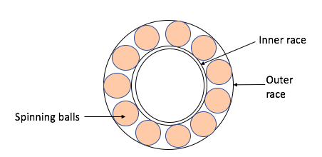
Figure 5: A schematic diagram of a ball bearing and the location of the three faults ((b) inner race, (c) outer race, and (d) ball spin).

A commonly used analytic tool in vibration analysis is the envelope spectrum. This is where a smoothing filter is applied to the regular periodogram to extract the dominant frequencies. Using the envelope spectrum, Randall and Antoni (2011) and Smith and Randall (2015), have shown that a normal ball bearing has power distributed in the relatively lower frequency bandwidth of $60-150$ Hz ($0.05-0.1$, radian). Whereas, faults in the ball bearings lead to deviation from the usual spectral distribution with significant power in the $300-500$ Hz ($0.18-0.26$, radian) bandwidth, depending on the location of the fault. Note that the following are equally important in a vibration analysis, frequencies where the power is greatest but also the amplitude of the power at these frequencies.

The time series in the repository are extremely long, of the order $10^{6}$. But as the ultimate aim is to devise an online detection scheme based on shorter time series, we focus on shorter segments of the time series ($n=609$, approximately $0.05$ seconds). A plot of the four different time series is given in Figure 6. In this study, we estimate the spectral density of the four time series signals by smoothing the different periodograms; regular, tapered, complete, and tapered complete periodogram. Our aim is to highlight the differences in the dominant frequencies in the spectral distribution of the normal ball bearing signal with three faulty signals. For the tapered and the tapered complete periodogram, we use the Tukey taper defined in (2.20) with $10\%$ tapering (which corresponds to $d=n/10$). For all the periodograms we smooth using the Bartlett window. For the time series (length $609$) we used $m=16$ (where $m$ is defined in Section 4.2).

A plot of the estimated spectral densities is given in Figure 7. We observe that all the four spectral density estimators (based on the different periodograms) are very similar. Further, for the normal ball bearing the main power is in the frequency range $0.05-0.1(60-175\text{ Hz})$. Interestingly, the spectral density estimator based on the tapered complete periodogram gives a larger amplitude at the principal frequency. Suggesting that the“normal signal” has greater power at that main frequency than is suggested by the other estimation methods. In contrast, for the faulty ball bearings, the power spectrum is very different from the normal signal. Most of the dominant frequencies are in the range $0.21-0.26(375-490\text{ Hz})$. There appears to be differences between the power spectrum of the three different faults, but the difference is not as striking as the difference between no fault and fault. Whether the differences between the faults are statistically significant will be an avenue of future investigation. These observations corroborate the findings of the previous analysis of similar data, see for example Smith and Randall (2015). Despite the similarities in the different estimators the smooth tapered complete periodogram appears to better capture the dominant frequencies in the normal ball bearing. This is reassuring as one objective in vibration analysis is the estimation of power of the vibration at the dominant frequencies.

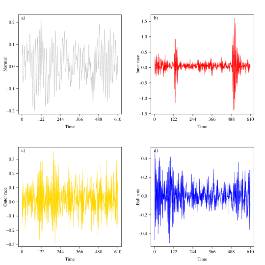
Figure 6: Panels in the figure show time series plots of signals recorded from a) Normal ball bearing b) Time series of bearing with fault in inner race, c) Time series of bearing with fault in outer race and, d) Time series of bearing with fault in ball spin. Each time series is of length $609$ (0.05 seconds).

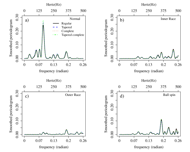
Figure 7: Plots show that smoothed periodograms of the four time series signals based on sample size $n=609$. Top left: Normal, Top Right: Inner Race, Bottom Left: Outer Race and Bottom Right: Ball spin. The top axis shows frequencies in Hertz(Hz).

Dedication and acknowledgements

This special issue of the Journal of Time Series Analysis is dedicated to the memory of Murray Rosenblatt who made many fundamental contributions time series analysis. The focus of this paper is on the role of the periodogram in analyzing second order stationary time series. However, generalisations of the periodogram can be used to analyze high order dependence structures, which was first proposed by Rosenblatt. In order to analyze higher order dependency within a time series, Rosenblatt (1966) and Brillinger and Rosenblatt (1967) (see Brillinger (1981)) introduced the $k$th-order periodogram, which is used to estimate the $k$th order spectral density. Indeed Brillinger and Rosenblatt (1967) and Bloomfield (2004), Section 6.5, use the $3$rd order periodogram to analyze the classica; sunspot data. The higher order spectra were subsequently used in Subba Rao and Gabr (1980, 1984) to discriminate between linear and nonlinear processes and to distinguish different types of nonlinear behaviour (see, also, Zhang and Wu (2018)).

SSR and JY gratefully acknowledge the partial of the National Science Foundation (grant DMS-1812054). SD would like to acknowledge an internal James Cook University seed grant that facilitated a collaborative visit to Texas A&M University. The authors thank Dr. Rainer Dahlhaus for his suggestions on tapering in time series. The authors are extremely gratefully to the comments and corrections made by two anonymous referees.

Summary of results in the Supplementary material

To navigate the supplementary material, we briefly summarize the contents of each section.

• In Appendix A, we prove the results in the main paper.

• In Appendix A.1, we prove Theorems 2.1$-$2.3. In particular obtaining bounds for $[\widehat{J}_{\infty,n}(\omega;f)-\widehat{J}_{n}(\omega;f)]\overline{J_{n}(\omega)}$, $[\widehat{J}_{\infty,n}(\omega;f)-\widehat{J}_{n}(\omega;f_{p})]\overline{J_{n}(\omega)}$ and $[\widehat{J}_{n}(\omega;f_{p})-\widehat{J}_{n}(\omega;\widehat{f}_{p})]\overline{J_{n}(\omega)}$. The first two bounds use Baxter-type lemmas. The last bound is prehaps the most challanging as it also involves estimators of the AR$(p)$ parameters.

• Appendix A.2 mainly concerns the integrated-type periodogram introduced in Section 3. In particular, in the proof of Theorem 3.1 we show that by using a weighted sum over the frequencies we can improve on some of the rates for the estimated complete periodogram at just one frequency.

• In Appendix A.3, we prove two technical lemmas required in the proof of Theorems 2.3 and 3.1.

• In Appendix B, we present additional simulations. Further we analysis the classical sunspot data using the estimated complete periodogram.

Appendix A Proofs

A.1 Proof of Theorems 2.1$-$2.3

Our aim in this section is to prove Theorems 2.1$-$2.3. To prove Theorem 2.1, we use the following results which show that $\widehat{J}_{\infty,n}(\omega;f)$ is the truncated version of the best infinite predictor.

We recall that $\widehat{X}_{\tau,n}$ is the best linear predictor of $X_{\tau}$ given $\{X_{t}\}_{t=1}^{n}$. We now extend the domain of prediction and consider the best linear predictor of $X_{\tau}$ ($\tau\leq 0$) given the infinite future $\{X_{t}\}_{t=1}^{\infty}$

$$\widehat{X}_{\tau}=\sum_{t=1}^{\infty}\phi_{t}(\tau;f)X_{t}$$

and, similarly, the best linear predictor of $X_{\tau}$ ($\tau>n$) given the infinite past $\{X_{t}\}_{t=-\infty}^{n}$

$$\widehat{X}_{\tau}=\sum_{t=1}^{\infty}\phi_{t}(\tau;f)X_{n+1-t}.$$

For future reference we will use the well known result that

$$\phi_{t}(\tau;f)=\sum_{s=0}^{\infty}a_{t+s}b_{|\tau|-s}\qquad t\geq 1,$$ (A.1)

where $\{a_{j}\}$ and $\{b_{j}\}$ are the AR$(\infty)$ and MA$(\infty)$ coefficients corresponding to the spectral density $f$ (we set $b_{s}=0$ for $s<0$). Thus if $n$ is large, then it seems reasonable to suppose that the best finite predictors are very close to the best infinite predictors truncated to the observed regressors i.e.

$$\widehat{X}_{\tau,n}\approx\sum_{t=1}^{n}\phi_{t}(\tau;f)X_{t}\textrm{ (for }\tau\leq 0)\quad\textrm{and}\quad\widehat{X}_{\tau,n}\approx\sum_{t=1}^{n}\phi_{n+1-t}(n-\tau;f)X_{t}\textrm{ (for }\tau>n).$$

Thus by defining $\widetilde{X}_{\tau,n}=\sum_{t=1}^{n}\phi_{t}(\tau;f)X_{t}$ (for $\tau\leq 0$) and $\widetilde{X}_{\tau,n}=\sum_{t=1}^{n}\phi_{n+1-t}(n-\tau;f)X_{t}$ (for $\tau>n$), and replacing the true finite predictions $\widehat{X}_{\tau,n}$ with their approximations we can obtain an approximation of $\widehat{J}_{n}(\omega;f)$. Indeed by using (A.1) we can show that this approximation is exactly $\widehat{J}_{\infty,n}(\omega;f)$. That is

$$\widehat{J}_{\infty,n}(\omega;f) = \frac{n^{-1/2}}{a(\omega;f)}\sum_{\ell=1}^{n}X_{\ell}\sum_{s=0}^{\infty}a_{\ell+s}e^{-is\omega}+e^{in\omega}\frac{n^{-1/2}}{\overline{a(\omega;f)}}\sum_{\ell=1}^{n}X_{n+1-\ell}\sum_{s=0}^{\infty}a_{\ell+s}e^{i(s+1)\omega}$$ (A.2)

$$= n^{-1/2}\sum_{\tau=-\infty}^{0}\widetilde{X}_{\tau,n}e^{i\tau\omega}+n^{-1/2}\sum_{\tau=n+1}^{\infty}\widetilde{X}_{\tau,n}e^{i\tau\omega}$$

$$= n^{-1/2}\sum_{t=1}^{n}X_{t}\big{(}\sum_{\tau\leq 0}\left[\phi_{t}(\tau;f)e^{i\tau\omega}+\phi_{n+1-t}(\tau;f)e^{-i(\tau-1-n)\omega}\right]\big{)}.$$

The above representation is an important component in the proof below.

Theorem A.1

Suppose Assumption 2.1 holds. Let $\widehat{J}_{n}(\omega;f)$, $\widehat{J}_{\infty,n}(\omega;f)$ and $\widehat{J}_{\infty,n}(\omega;f_{p})$ (where $f_{p}$ denotes the spectral density corresponding to the best fitting AR$(p)$ model) be defined as in (1.2), (2.3) and (2.2). Then we have

$$\mathbb{E}\left[\left(\widehat{J}_{\infty,n}(\omega;f)-\widehat{J}_{n}(\omega;f)\right)\overline{J_{n}(\omega)}\right] = O\left(n^{-K}\right),$$ (A.3)

$$\mathrm{var}\left[\left(\widehat{J}_{\infty,n}(\omega;f)-\widehat{J}_{n}(\omega;f)\right)\overline{J_{n}(\omega)}\right] = O\left(n^{-2K}\right),$$ (A.4)

$$\mathbb{E}\left[\left(\widehat{J}_{n}(\omega;f_{p})-\widehat{J}_{\infty,n}(\omega;f)\right)\overline{J_{n}(\omega)}\right] = O\left((np^{K-1})^{-1}\right)$$ (A.5)

and

$$\mathrm{var}\left[\left(\widehat{J}_{n}(\omega;f_{p})-\widehat{J}_{\infty,n}(\omega;f)\right)\overline{J_{n}(\omega)}\right] = O\left((np^{K-1})^{-2}\right).$$ (A.6)

PROOF. We first prove (A.3) and (A.4). We recall that

$$\widehat{J}_{n}(\omega;f) = n^{-1/2}\sum_{\tau=-\infty}^{0}\widehat{X}_{\tau,n}e^{i\tau\omega}+n^{-1/2}\sum_{\tau=n+1}^{\infty}\widehat{X}_{\tau,n}e^{i\tau\omega}$$

$$= n^{-1/2}\sum_{t=1}^{n}X_{t}\big{(}\sum_{\tau\leq 0}\left[\phi_{t,n}(\tau;f)e^{i\tau\omega}+\phi_{n+1-t,n}(\tau;f)e^{-i(\tau-1-n)\omega}\right]\big{)}$$

Using the above we write $\widehat{J}_{n}(\omega;f)$ as an innerproduct. Let

$$D_{t,n}(f)=n^{-1/2}\sum_{\tau\leq 0}\left[\phi_{t,n}(\tau;f)e^{i\tau\omega}+\phi_{n+1-t,n}(\tau;f)e^{-i(\tau-1-n)\omega}\right].$$

Next, define the vectors

$$\underline{e}_{n}^{\prime}=n^{-1/2}(e^{-i\omega},...,e^{-in\omega})\quad\text{and}\quad\underline{D}_{n}(f)^{\prime}=(D_{1,n}(f),...,D_{n,n}(f)),$$

note that $\underline{e}_{n}$ and $\underline{D}_{n}(f)$ are both functions of $\omega$, but we have surpressed this dependence in our notation. Then, $J_{n}(\omega)$ and $\widehat{J}_{n}(\omega;f)$ can be represented as the inner products

$$J_{n}(\omega)=\underline{e}_{n}^{\ast}\underline{X}_{n}\textrm{ and }\widehat{J}_{n}(\omega;f)=\underline{X}_{n}^{\prime}\underline{D}_{n}(f)$$

where $\ast$ denotes the Hermitian of a matrix. In the same vein we write $\widehat{J}_{\infty,n}(\omega;f)$ as an innerproduct. We recall from (A.2) that

$$\widehat{J}_{\infty,n}(\omega;f)=n^{-1/2}\sum_{t=1}^{n}X_{t}\big{(}\sum_{\tau\leq 0}\left[\phi_{t}(\tau;f)e^{i\tau\omega}+\phi_{n+1-t}(\tau;f)e^{-i(\tau-1-n)\omega}\right]\big{)}.$$ (A.7)

As above, let

$$D_{t}(f) = n^{-1/2}\sum_{\tau\leq 0}\left[\phi_{t}(\tau;f)e^{i\tau\omega}+\phi_{n+1-t}(\tau;f)e^{-i(\tau-1-n)\omega}\right]$$

$$\underline{D}_{\infty,n}(f)^{\prime} = (D_{1}(f),...,D_{n}(f)),$$

then we can write $\widehat{J}_{\infty,n}(\omega;f)=\underline{X}_{n}^{\prime}\underline{D}_{n}(f)$. Therefore,

$$\left(\widehat{J}_{\infty,n}(\omega;f)-\widehat{J}_{n}(\omega;f)\right)\overline{J_{n}(\omega)} = I_{\infty,n}(\omega;f)-I_{n}(\omega;f)$$

$$= n^{-1/2}\sum_{s,t=1}^{n}X_{t}X_{s}(\underline{D}_{\infty,n}(f)-\underline{D}_{n}(f))_{(t)}e^{-is\omega}$$

$$= \underline{X}_{n}^{\prime}\left(\underline{D}_{\infty,n}(f)-\underline{D}_{n}(f)\right)\underline{e}_{n}^{\prime}\underline{X}_{n}$$

$$= \underline{X}_{n}^{\prime}A_{1}(\omega)\underline{X}_{n}$$

where $A_{1}(\omega)=\left(\underline{D}_{\infty,n}(f)-\underline{D}_{n}(f)\right)\underline{e}_{n}^{\prime}$, an $(n\times n)$ matrix. For the remainder of this proof we drop the dependence of $A_{1}(\omega)$ on $\omega$. However, if we integrate over $\omega$ this dependence does become important. Using this notation, we have

$$\mathbb{E}\left[\left(\widehat{J}_{\infty,n}(\omega;f)-\widehat{J}_{n}(\omega;f)\right)\overline{J_{n}(\omega)}\right] = \mathbb{E}[\underline{X}_{n}^{\prime}A_{1}\underline{X}_{n}]$$

$$\mathrm{var}\left[\left(\widehat{J}_{\infty,n}(\omega;f)-\widehat{J}_{n}(\omega;f)\right)\overline{J_{n}(\omega)}\right] = \mathrm{var}[\underline{X}_{n}^{\prime}A_{1}\underline{X}_{n}].$$

By simple algebra

$$\mathbb{E}[\underline{X}_{n}^{\prime}A_{1}\underline{X}_{n}] = {\rm tr}(A_{1}R_{n})$$

$$\mathrm{var}[\underline{X}_{n}^{\prime}A_{1}\underline{X}_{n}] = 2{\rm tr}(A_{1}R_{n}A_{1}R_{n})+\sum_{s,t,u,v=1}^{n}(A_{1})_{s,t}(A_{1})_{u,v}\mathrm{cum}\left(X_{s},X_{t},X_{u},X_{v}\right),$$ (A.8)

where $R_{n}=\mathrm{var}[\underline{X}_{n}]$ (noting that $R_{n}$ is a Toeplitz matrix). To bound the expectation

$$\left|\mathbb{E}[\underline{X}_{n}^{\prime}A_{1}\underline{X}_{n}]\right|=|{\rm tr}(A_{1}R_{n})| \leq n^{-1/2}\sum_{s,t=1}^{n}|(\underline{D}_{\infty,n}(f)-\underline{D}_{n}(f))_{(t)}e^{-is\omega}(R_{n})_{t,s}|$$ (A.9)

$$= n^{-1/2}\sum_{s,t=1}^{n}|D_{t}(f)-D_{t,n}(f)||c(t-s)|$$

$$\leq n^{-1/2}\sum_{t=1}^{n}|D_{t}(f)-D_{t,n}(f)|\left(\sum_{r\in\mathbb{Z}}|c(r)|\right).$$

To bound the above, we observe that the sum over $t$ is

$$n^{-1/2}\sum_{t=1}^{n}|D_{t}(f)-D_{t,n}(f)|$$

$$\quad=n^{-1}\sum_{t=1}^{n}\sum_{\tau\leq 0}\left|(\phi_{t}(\tau;f)-\phi_{t,n}(\tau;f))e^{i\tau\omega}+(\phi_{n+1-t}(\tau;f)-\phi_{n+1-t,n}(\tau;f))e^{-i(\tau-1-n)\omega}\right|$$

$$\quad\leq n^{-1}\sum_{t=1}^{n}\sum_{\tau\leq 0}|\phi_{t}(\tau;f)-\phi_{t,n}(\tau;f)|+\sum_{t=1}^{n}\sum_{\tau\leq 0}|\phi_{n+1-t}(\tau;f)-\phi_{n+1-t,n}(\tau;f)|$$

$$\quad=2n^{-1}\sum_{t=1}^{n}\sum_{\tau\leq 0}|\phi_{t}(\tau;f)-\phi_{t,n}(\tau;f)|.$$

To bound the above, we use the generalized Baxter’s inequality, SY20, Lemma B.1, which for completeness we now state. For sufficiently large $n$ we have the bound

$$\sum_{s=1}^{n}(2^{K}+s^{K})\left|\phi_{s,n}(\tau;f)-\phi_{s}(\tau;f)\right|\leq C_{f,K}\sum_{s=n+1}^{\infty}(2^{K}+s^{K})\left|\phi_{s}(\tau;f)\right|,$$ (A.10)

where $C_{f,K}$ is a finite constant that only depends on $f$ and $K$. Using (A.10) with $K=0$ and (A.1) we have

$$\sum_{t=1}^{n}\sum_{\tau\leq 0}|\phi_{t}(\tau;f)-\phi_{t,n}(\tau;f)| \leq C_{f,0}\sum_{\tau\leq 0}\sum_{t=n+1}^{\infty}|\phi_{t}(\tau;f)|$$

$$\leq C_{f,0}\sum_{\tau=0}^{\infty}\sum_{t=n+1}^{\infty}\sum_{j=0}^{\infty}|a_{t+j}||b_{\tau-j}|\leq C_{f,0}\sum_{\ell\in\mathbb{Z}}|b_{\ell}|\sum_{t=n+1}^{\infty}\sum_{j=0}^{\infty}|a_{t+j}|$$

$$\leq C_{f,0}\sum_{\ell\in\mathbb{Z}}|b_{\ell}|\sum_{u=n+1}^{\infty}|ua_{u}|\leq\frac{C_{f,0}}{n^{K-1}}\sum_{\ell\in\mathbb{Z}}|b_{\ell}|\sum_{u=n+1}^{\infty}|u^{K}a_{u}|$$

To bound the above we use Assumption 2.1. By using Lemma 2.1 of Kreiss et al. [2011], under Assumption 2.1, we have $\sum_{u=1}^{\infty}|u^{K}a_{u}|\leq\infty$. Therefore,

$$\sum_{t=1}^{n}\sum_{\tau\leq 0}|\phi_{t}(\tau;f)-\phi_{t,n}(\tau;f)|=O(n^{-K+1}),$$

which gives

$$n^{-1/2}\sum_{t=1}^{n}|D_{t}(f)-D_{t,n}(f)|\leq 2n^{-1}\sum_{t=1}^{n}\sum_{\tau\leq 0}|\phi_{t}(\tau;f)-\phi_{t,n}(\tau;f)|=O(n^{-K}).$$ (A.11)

Substituting the above bound into (A.9) gives

$$\mathbb{E}[\underline{X}_{n}^{\prime}A_{1}\underline{X}_{n}]={\rm tr}(A_{1}R_{n})\leq n^{-1/2}\sum_{t=1}^{n}|D_{t}(f)-D_{t,n}(f)|\left(\sum_{r\in\mathbb{Z}}|c(r)|\right)=O(n^{-K}).$$ (A.12)

Next we consider the variance. The first term in the variance (A.8) is bounded with

$$|{\rm tr}(A_{1}R_{n}A_{1}R_{n})| \leq n^{-1}\sum_{s,t,u,v=1}^{n}|(D_{s}(f)-D_{s,n}(f))(D_{t}(f)-D_{t,n}(f))e^{-iu\omega}e^{-iv\omega}(R_{n})_{s,u}(R_{n})_{t,v}|$$

$$= n^{-1}\sum_{s,t,u,v=1}^{n}|D_{s}(f)-D_{s,n}(f)||D_{t}(f)-D_{t,n}(f)||c(s-u)||c(t-v)|$$

$$\leq \left(n^{-1/2}\sum_{t=1}^{n}|D_{t}(f)-D_{t,n}(f)|\right)^{2}\left(\sum_{r\in\mathbb{Z}}|c(r)|\right)^{2}=O(n^{-2K}),$$

where the last line follows from (A.11). The second term in (A.8) is bounded by

$$\sum_{s,t,u,v=1}^{n}|(A_{1})_{s,t}(A_{1})_{u,v}\mathrm{cum}\left(X_{s},X_{t},X_{u},X_{v}\right)|$$

$$\quad=n^{-1}\sum_{s,t,u,v=1}^{n}|D_{t}(f)-D_{t,n}(f)||D_{v}(f)-D_{v,n}(f)|\kappa_{4}\left(t-s,u-s,v-s\right)|$$

$$\quad\leq n^{-1}\sum_{t,v=1}^{n}|D_{t}(f)-D_{t,n}(f)||D_{v}(f)-D_{v,n}(f)|\sum_{s,u=1}^{n}|\kappa_{4}\left(t-s,u-s,v-s\right)|$$

$$\quad\leq n^{-1}\sum_{t,v=1}^{n}|D_{t}(f)-D_{t,n}(f)||D_{v}(f)-D_{v,n}(f)|\sum_{i,j,k\in\mathbb{Z}}|\kappa_{4}\left(i,j,k\right)|$$

$$\quad=\left(n^{-1/2}\sum_{t=1}^{n}|D_{t}(f)-D_{t,n}(f)|\right)^{2}\sum_{i,j,k\in\mathbb{Z}}|\kappa_{4}\left(i,j,k\right)|=O\left(n^{-2K}\right)$$

where the above follows from (A.11) and Assumption 2.2. Altogether this gives $\mathrm{var}[\underline{X}_{n}^{\prime}A_{1}\underline{X}_{n}]=O(n^{-2K})$. This proves (A.3) and (A.4).

To prove (A.5) and (A.6) we use the following observation. In the special case that $f=f_{p}$ corresponds to the AR$(p)$ model, the best finite linear predictor (given $p$ observations) and the best infinite predictor are the same in this case, $\underline{D}_{n}(f_{p})=\underline{D}_{\infty,n}(f_{p})$. Therefore, we have

$$\left(\widehat{J}_{n}(\omega;f_{p})-\widehat{J}_{\infty,n}(\omega;f)\right)\overline{J_{n}(\omega)} = n^{-1/2}\sum_{s,t=1}^{n}X_{s}X_{t}(\underline{D}_{\infty,n}(f)-\underline{D}_{n}(f_{p}))_{(t)}e^{-is\omega}$$ (A.13)

$$= \underline{X}_{n}^{\prime}\left(\underline{D}_{\infty,n}(f_{p})-\underline{D}_{\infty,n}(f)\right)\underline{e}_{n}^{\prime}\underline{X}_{n}$$

$$= \underline{X}_{n}^{\prime}A_{2}(\omega)\underline{X}_{n}$$

where $A_{2}(\omega)=\left(\underline{D}_{\infty,n}(f_{p})-\underline{D}_{\infty,n}(f)\right)\underline{e}_{n}^{\prime}$. Again we drop the dependence of $A_{2}$ on $\omega$, but it will play a role in the proof of Theorem 3.1. To bound the mean and variance of $\underline{X}_{n}^{\prime}A_{2}\underline{X}_{n}$ we use similar expressions to (A.8). Thus by using the same method described above leads to our requiring bounds for

$$\left|\mathbb{E}[\underline{X}_{n}^{\prime}A_{2}\underline{X}_{n}]\right|\leq n^{-1/2}\sum_{t=1}^{n}|D_{t}(f_{p})-D_{t}(f)|\left(\sum_{r\in\mathbb{Z}}|c(r)|\right)$$ (A.14)

$$|{\rm tr}(A_{2}R_{n}A_{2}R_{n})|\leq\left(n^{-1/2}\sum_{t=1}^{n}|D_{t}(f_{p})-D_{t}(f)|\right)^{2}\left(\sum_{r\in\mathbb{Z}}|c(r)|\right)^{2}$$

$$\sum_{s,t,u,v=1}^{n}|(A_{2})_{s,t}(A_{2})_{u,v}\mathrm{cum}\left(X_{s},X_{t},X_{u},X_{v}\right)|\leq\left(n^{-1/2}\sum_{t=1}^{n}|D_{t}(f_{p})-D_{t}(f)|\right)^{2}\sum_{i,j,k\in\mathbb{Z}}|\kappa_{4}\left(i,j,k\right)|.$$

The above three bounds require a bound for $\sum_{t=1}^{n}|D_{t}(f_{p})-D_{t}(f)|$. To obtain such a bound we recall from (A.1) that

$$\phi_{t}(\tau;f)=\sum_{j=0}^{\infty}a_{t+j}b_{|\tau|-j}\qquad\phi_{t}(\tau;f_{p})=\sum_{j=0}^{\infty}a_{t+j,p}b_{|\tau|-j,p}$$

where $\{a_{s}\}_{s=1}^{\infty}$, $\{a_{s,p}\}_{s=1}^{p}$, $\{b_{j}\}_{j=0}^{\infty}$ and $\{b_{j,p}\}_{j=0}^{\infty}$ are the AR$(\infty)$, AR$(p)$ and MA$(\infty)$ coefficients corresponding to the spectral density $f$ and $f_{p}$ respectively. Taking differences gives

$$n^{-1/2}\sum_{t=1}^{n}|D_{t}(f)-D_{t}(f_{p})| \leq 2n^{-1}\sum_{t=1}^{n}\sum_{\tau\leq 0}\left|\phi_{t}(\tau;f)-\phi_{t}(\tau;f_{p})\right|$$

$$\leq 2n^{-1}\sum_{t=1}^{n}\sum_{\tau\leq 0}\sum_{j=0}^{\infty}\left|a_{t+j}b_{|\tau|-j}-a_{t+j,p}b_{|\tau|-j,p}\right|$$

$$\leq 2n^{-1}\sum_{t=1}^{n}\sum_{\tau\leq 0}\sum_{j=0}^{\infty}\left|a_{t+j}-a_{t+j,p}\right||b_{|\tau|-j}|$$

$$+2n^{-1}\sum_{t=1}^{n}\sum_{\tau\leq 0}\sum_{j=0}^{\infty}\left|b_{|\tau|-j}-b_{|\tau|-j,p}\right||a_{t+j,p}|=I_{1}+I_{2}.$$

We consider first term $I_{1}$. Reordering the summands gives

$$I_{1} = 2n^{-1}\sum_{t=1}^{n}\sum_{j=0}^{\infty}\left|a_{t+j}-a_{t+j,p}\right|\sum_{\tau\leq 0}|b_{|\tau|-j}|$$

$$\leq 2n^{-1}\sum_{\ell=0}^{\infty}|b_{\ell}|\sum_{t=1}^{n}\sum_{j=0}^{\infty}\left|a_{t+j}-a_{t+j,p}\right|\qquad(\textrm{let }u=t+j)$$

$$\leq 2n^{-1}\sum_{\ell=0}^{\infty}|b_{\ell}|\sum_{u=0}^{\infty}u\left|a_{u}-a_{u,p}\right|.$$

By applying the Baxter’s inequality to the above we have

$$I_{1} \leq 2(1+C)n^{-1}\sum_{\ell=0}^{\infty}|b_{\ell}|\sum_{u=p+1}^{\infty}|ua_{u}|=O\left(\frac{1}{np^{K-1}}\right).$$

To bound $I_{2}$ we use a similar method

$$I_{2} = 2n^{-1}\sum_{\tau\geq 0}\sum_{j=0}^{\infty}\left|b_{\tau-j}-b_{\tau-j,p}\right|\sum_{t=1}^{n}|a_{t+j,p}|$$

$$\leq 2n^{-1}\sum_{t=1}^{p}|a_{t,p}|\sum_{u=0}^{\infty}u\left|b_{u}-b_{u,p}\right|.$$

By using the inequality on page 2126 of Kreiss et al. [2011], for a large enough $n$, we have $\sum_{u=0}^{\infty}u|b_{u}-b_{u,p}|\leq C\sum_{u=p+1}^{\infty}|ua_{u}|=O(p^{-K+1})$. Substituting this into the above gives

$$I_{2}\leq Cn^{-1}\sum_{t=1}^{p}|a_{t,p}|\sum_{u=p+1}^{\infty}|ua_{u}|=O\left(\frac{1}{np^{K-1}}\right),$$

where we note that $\sup_{t}\sum_{t=1}^{p}|a_{t,p}|=O(1)$. Altogether this gives

$$n^{-1/2}\sum_{t=1}^{n}|D_{t}(f_{p})-D_{t}(f)| = O\left(\frac{1}{np^{K-1}}\right).$$

Substituting the above bound into (A.14) and using a similar proof to (A.3) and (A.4) we have

$$\mathbb{E}[\underline{X}_{n}^{\prime}A_{2}\underline{X}_{n}]=O\left(\frac{1}{np^{K-1}}\right)\quad\textrm{ and }\quad\mathrm{var}[\underline{X}_{n}^{\prime}A_{2}\underline{X}_{n}]=O\left(\frac{1}{n^{2}p^{2K-2}}\right).$$

This proves (A.5) and (A.6), which gives the required result. $\Box$

PROOF of Theorem 2.1. The proof immediately follows from Theorem A.1, equations (A.3) and (A.4). $\Box$

PROOF of Theorem 2.2. The proof immediately follows from Theorem A.1, equations (A.5) and (A.6). $\Box$

PROOF of equation (2.5) We note that

$$\widehat{J}_{n}(\omega;f)\overline{J_{n}(\omega)}=\left(\widehat{J}_{n}(\omega;f)-\widehat{J}_{\infty,n}(\omega;f)\right)\overline{J_{n}(\omega)}+\widehat{J}_{\infty,n}(\omega;f)\overline{J_{n}(\omega)}.$$

The mean and variance of the first term on the right hand side of the above was evaluated in Theorem A.1 and has a lower order. Now we focus on the second term. Using the notation from Theorem A.1 we have

$$\widehat{J}_{\infty,n}(\omega;f)\overline{J_{n}(\omega)} = \underline{X}_{n}^{\prime}\underline{D}_{\infty,n}(f)\underline{e}_{n}^{\prime}\underline{X}_{n}.$$

Thus by using the same methods as those given in (A.9) we have

$$\left|\mathbb{E}[\widehat{J}_{\infty,n}(\omega;f)\overline{J_{n}(\omega)}]\right| \leq n^{-1/2}\sum_{s,t=1}^{n}|(\underline{D}_{\infty,n}(f))_{(t)}e^{-is\omega}(R_{n})_{t,s}|$$

$$= n^{-1/2}\sum_{s,t=1}^{n}|D_{t}(f)||c(t-s)|$$

$$\leq n^{-1/2}\sum_{t=1}^{n}|D_{t}(f)|\left(\sum_{r\in\mathbb{Z}}|c(r)|\right)$$

$$\leq 2n^{-1}\sum_{t=1}^{n}\sum_{\tau\leq 0}|\phi_{t}(\tau;f)|\left(\sum_{r\in\mathbb{Z}}|c(r)|\right)=O(n^{-1}).$$

Following a similar argument for the variance we have $\mathrm{var}[\widehat{J}_{\infty,n}(\omega;f)\overline{J_{n}(\omega)}]=O(n^{-2})$ and this proves the equation (2.5) $\Box$

We now obtain a bound for the estimated complete DFT, this proof will use two technical lemmas that are given in Appendix A.3.

PROOF of Theorem 2.3. Consider the expansion

$$I_{n}(\omega;\widehat{f}_{p})-I_{n}(\omega,f_{p})=\left[\widehat{J}_{n}(\omega;\widehat{f}_{p})-\widehat{J}_{n}(\omega;f_{p})\right]\overline{J_{n}(\omega)}=E_{n}(\omega).$$

The main idea of the proof is to decompose $E_{n}(\omega)$ into terms whose expectation (and variance) can be evaluated plus an additional error whose expectation cannot be evaluated (since it involves ratios of random variables), but whose probabilistic bound is less than the expectation. We will make a Taylor expansion of the estimated parameters about the true parameters. The order of the Taylor expansion used will be determined by the order of summability of the cumulants in Assumption 2.2. For a given even $m$, the order of the Taylor expansion will be $(m/2-1)$. The reason for this will be clear in the proof, but roughly speaking we need to evaluate the mean and variance of the terms in the Taylor expansion. The higher the order of the expansion we make, the higher the cumulant asssumptions we require. To simplify the proof, we prove the result in the specific case that Assumption 2.2 holds for $m=8$ (summability of all cumulants up to the $16$th order). This, we will show, corresponds to making a third order Taylor expansion of the sample autocovariance function about the true autocovariance function. Note that the third order expansion requires summability of the $16$th-order cumulants.

We now make the above discussion precise. By using equation (2.2) and (2.11) we have

$$\widehat{J}_{n}(\omega;f_{p}) = \frac{n^{-1/2}}{a_{p}(\omega)}\sum_{\ell=1}^{p}X_{\ell}\sum_{s=0}^{p-\ell}a_{\ell+s}e^{-is\omega}+e^{in\omega}\frac{n^{-1/2}}{\overline{a_{p}(\omega)}}\sum_{\ell=1}^{p}X_{n+1-\ell}\sum_{s=0}^{p-\ell}a_{\ell+s}e^{i(s+1)\omega}$$

$$= \frac{1}{\sqrt{n}}\left(\sum_{\ell=1}^{p}X_{\ell}\frac{a_{\ell,p}(\omega)}{1-a_{0,p}(\omega)}+e^{i(n+1)\omega}\sum_{\ell=1}^{p}X_{n+1-\ell}\frac{\overline{a_{\ell,p}(\omega)}}{1-\overline{a_{0,p}(\omega)}}\right)$$

and

$$\widehat{J}_{n}(\omega;\widehat{f}_{p}) = \frac{1}{\sqrt{n}}\left(\sum_{\ell=1}^{p}X_{\ell}\frac{\widehat{a}_{\ell,p}(\omega)}{1-\widehat{a}_{0,p}(\omega)}+e^{i(n+1)\omega}\sum_{\ell=1}^{p}X_{n+1-\ell}\frac{\overline{\widehat{a}_{\ell,p}(\omega)}}{1-\overline{\widehat{a}_{0,p}(\omega)}}\right),$$

where for $\ell\geq 0$

$$a_{\ell,p}(\omega)=\sum_{s=0}^{p-\ell}a_{\ell+s}e^{-is\omega}\quad(a_{0}\equiv 0)$$

and $\widehat{a}_{\ell,p}(\omega)$ is defined similarly but with the estimated Yule-Walker coefficients. Therefore

$$\widehat{J}_{n}(\omega;f_{p})-\widehat{J}_{n}(\omega;f_{p})=E_{n}(\omega)$$

where

$$E_{n}(\omega) = \frac{1}{n}\sum_{t=1}^{n}\sum_{\ell=1}^{p}X_{\ell}X_{t}e^{it\omega}\left[\frac{\widehat{a}_{\ell,p}(\omega)}{1-\widehat{a}_{0,p}(\omega)}-\frac{a_{\ell,p}(\omega)}{1-a_{0,p}(\omega)}\right]$$

$$+e^{i(n+1)\omega}\frac{1}{n}\sum_{t=1}^{n}\sum_{\ell=1}^{p}X_{n+1-\ell}X_{t}e^{it\omega}\left[\frac{\overline{\widehat{a}_{\ell,p}(\omega)}}{1-\overline{\widehat{a}_{0,p}(\omega)}}-\frac{\overline{a_{\ell,p}(\omega)}}{1-\overline{a_{0,p}(\omega)}}\right]$$

$$= \frac{1}{n}\sum_{t=1}^{n}\sum_{\ell=1}^{p}X_{\ell}X_{t}e^{it\omega}\left[g_{\ell,p}(\omega,\widehat{\underline{c}}_{p,n})-g_{\ell,p}(\omega,\underline{c}_{p})\right]$$

$$+e^{i(n+1)\omega}\frac{1}{n}\sum_{t=1}^{n}\sum_{\ell=1}^{p}X_{n+1-\ell}X_{t}e^{it\omega}\left[\overline{g_{\ell,p}(\omega,\widehat{\underline{c}}_{p,n})}-\overline{g_{\ell,p}(\omega,\underline{c}_{p})}\right]$$

$$= E_{n,L}(\omega)+E_{n,R}(\omega),$$

where $\underline{c}_{p}^{\prime}=(c(0),c(1),\ldots,c(p))$, $\widehat{\underline{c}}_{p,n}^{\prime}=(\widehat{c}_{n}(0),\widehat{c}_{n}(1),\ldots,\widehat{c}_{n}(p))$,

$$g_{\ell,p}(\omega,\underline{c}_{p,n})=\frac{a_{\ell,p}(\omega)}{1-a_{0,p}(\omega)}\quad\text{and}\quad g_{\ell,p}(\omega,\widehat{\underline{c}}_{p,n})=\frac{\widehat{a}_{\ell,p}(\omega)}{1-\widehat{a}_{0,p}(\omega)}.$$ (A.15)

For the notational convenience, we denote by $\{c_{k}\}$ and $\{\widehat{c}_{k}\}$ the autocovariances and sample autocovariances of the time series respectively.

Let $(R_{p})_{s,t}=c(s-t)$, $(\underline{r}_{p})_{k}=c(k)$, $(\widehat{R}_{p})_{s,t}=\widehat{c}_{n}(s-t)$ and $(\widehat{\underline{r}}_{p})_{k}=\widehat{c}_{n}(k)$. Then since Since $\underline{a}_{p}=R_{p}^{-1}\underline{r}_{p}$ and $\underline{\widehat{a}}_{p}=\widehat{R}_{p,n}^{-1}\widehat{\underline{r}}_{p,n}$, an explicit expression for $g_{\ell,p}(\omega,\underline{c}_{p})$ and $g_{\ell,p}(\omega,\underline{\widehat{c}}_{p,n})$ is

$$g_{\ell,p}(\omega,\underline{c}_{p})=\frac{\underline{r}_{p}^{\prime}R_{p}^{-1}\underline{e}_{\ell}(\omega)}{1-\underline{r}_{p}^{\prime}R_{p}^{-1}\underline{e}_{0}(\omega)}\quad\text{and}\quad g_{\ell,p}(\omega,\widehat{\underline{c}}_{p,n})=\frac{\widehat{\underline{r}}_{p,n}^{\prime}\widehat{R}_{p,n}^{-1}\underline{e}_{\ell}(\omega)}{1-\widehat{\underline{r}}_{p,n}^{\prime}\widehat{R}_{p,n}^{-1}\underline{e}_{0}(\omega)},$$ (A.16)

where $\underline{e}_{\ell}(\omega)$ are $p$-dimension vectors, with

$$\underline{e}_{\ell}(\omega)^{\prime}=(\underbrace{0,\ldots,0}_{\ell-\textrm{zeros}},e^{-i\omega},\ldots,e^{-i(p-\ell)\omega})\textrm{ for }0\leq\ell\leq p.$$ (A.17)

Since $E_{n,L}(\omega)$ and $E_{n,R}(\omega)$ are near identical expressions, we will only study $E_{n,L}(\omega)$, noting the same analysis and bounds also apply to $E_{n,R}(\omega)$. We observe that the random functions $\widehat{a}_{\ell,p}(\omega)$ form the main part of $E_{n,L}(\omega)$. $\widehat{a}_{\ell,p}(\omega)$ are rather complex and directly evaluating their mean and variance is extremely difficult if not impossible. However, on careful examination we observe that they are functions of the autocovariance function whose sampling properties are well known. For this reason, we make a third order Taylor expansion of $g_{\ell,p}(\omega,\widehat{\underline{c}}_{p,n})$ about $g_{\ell,p}(\omega,\underline{c}_{p})$:

$$g_{\ell,p}(\omega,\widehat{\underline{c}}_{p,n})-g_{\ell,p}(\omega,\underline{c}_{p}) = \sum_{j=0}^{p}\left(\widehat{c}_{j}-c_{j}\right)\frac{\partial g_{\ell,p}(\omega,\underline{c}_{p})}{\partial c_{j}}+\frac{1}{2!}\sum_{j_{1},j_{2}=0}^{p}\left(\widehat{c}_{j_{1}}-c_{j_{1}}\right)\left(\widehat{c}_{j_{2}}-c_{j_{2}}\right)\frac{\partial^{2}g_{\ell,p}(\omega,\underline{c}_{p})}{\partial c_{j_{1}}\partial c_{j_{2}}}$$

$$+\frac{1}{3!}\sum_{j_{1},j_{2},j_{3}=0}^{p}\left(\widehat{c}_{j_{1}}-c_{j_{1}}\right)\left(\widehat{c}_{j_{2}}-c_{j_{2}}\right)\left(\widehat{c}_{j_{3}}-c_{j_{3}}\right)\frac{\partial^{3}g_{\ell,p}(\omega,\underline{\widetilde{c}}_{p,n})}{\partial\widetilde{c}_{j_{1}}\partial\widetilde{c}_{j_{2}}\partial\widetilde{c}_{j_{3}}}$$

where $\widetilde{\underline{c}}_{p,n}$ is a convex combination of $\underline{c}_{p}$ and $\widehat{\underline{c}}_{p,n}$. Such an expansion draws the sample autocovariance function out of the sum, allowing us to evaluate the mean and variance for the first and second term. Substituting the third order expansion into $E_{n,L}(\omega)$ gives the sum

$$E_{n,L}(\omega) = \underbrace{E_{11}(\omega)+E_{12}(\omega)+E_{21}(\omega)+E_{22}(\omega)}_{=\Delta_{2,L}(\omega)}+\underbrace{E_{31}(\omega)+E_{32}(\omega)}_{=R_{L}(\omega)},$$

where

$$E_{11}(\omega) = \sum_{j=0}^{p}\sum_{\ell=1}^{p}\frac{1}{n}\sum_{t=1}^{n}\left(X_{\ell}X_{t}-\mathbb{E}[X_{\ell}X_{t}]\right)e^{it\omega}\left(\widehat{c}_{j}-c_{j}\right)\frac{\partial g_{\ell,p}(\omega,\underline{c}_{p})}{\partial c_{j}}$$

$$E_{12}(\omega) = \sum_{j=0}^{p}\sum_{\ell=1}^{p}\frac{1}{n}\sum_{t=1}^{n}\mathbb{E}[X_{\ell}X_{t}]e^{it\omega}\left(\widehat{c}_{j}-c_{j}\right)\frac{\partial g_{\ell,p}(\omega,\underline{c}_{p})}{\partial c_{j}}$$

$$E_{21}(\omega) = \frac{1}{2}\sum_{j_{1},j_{2}=0}^{p}\sum_{\ell=1}^{p}\frac{1}{n}\sum_{t=1}^{n}\left(X_{\ell}X_{t}-\mathbb{E}[X_{\ell}X_{t}]\right)e^{it\omega}\left(\widehat{c}_{j_{1}}-c_{j_{1}}\right)\left(\widehat{c}_{j_{2}}-c_{j_{2}}\right)\frac{\partial^{2}g_{\ell,p}(\omega,\underline{c}_{p})}{\partial c_{j_{1}}\partial c_{j_{2}}}$$

$$E_{22}(\omega) = \frac{1}{2}\sum_{j_{1},j_{2}=0}^{p}\sum_{\ell=1}^{p}\frac{1}{n}\sum_{t=1}^{n}\mathbb{E}[X_{\ell}X_{t}]e^{it\omega}\left(\widehat{c}_{j_{1}}-c_{j_{1}}\right)\left(\widehat{c}_{j_{2}}-c_{j_{2}}\right)\frac{\partial^{2}g_{\ell,p}(\omega,\underline{c}_{p})}{\partial c_{j_{1}}\partial c_{j_{2}}}$$

and

$$E_{31}(\omega) = \frac{1}{3!}\sum_{j_{1},j_{2}=0}^{p}\sum_{\ell=1}^{p}\frac{1}{n}\sum_{t=1}^{n}\left(X_{\ell}X_{t}-\mathbb{E}[X_{\ell}X_{t}]\right)e^{it\omega}\left(\widehat{c}_{j_{1}}-c_{j_{1}}\right)\left(\widehat{c}_{j_{2}}-c_{j_{2}}\right)\left(\widehat{c}_{j_{3}}-c_{j_{3}}\right)\frac{\partial^{3}g_{\ell,p}(\omega,\underline{\widetilde{c}}_{p,n})}{\partial\widetilde{c}_{j_{1}}\partial\widetilde{c}_{j_{2}}\partial\widetilde{c}_{j_{3}}}$$

$$E_{32}(\omega) = \frac{1}{3!}\sum_{j_{1},j_{2},j_{3}=0}^{p}\sum_{\ell=1}^{p}\frac{1}{n}\sum_{t=1}^{n}\mathbb{E}[X_{\ell}X_{t}]e^{it\omega}\left(\widehat{c}_{j_{1},n}-c_{j_{1}}\right)\left(\widehat{c}_{j_{2}}-c_{j_{2}}\right)\left(\widehat{c}_{j_{3}}-c_{j_{3}}\right)\frac{\partial^{3}g_{\ell,p}(\omega,\underline{\widetilde{c}}_{p})}{\partial\widetilde{c}_{j_{1}}\partial\widetilde{c}_{j_{2}}\partial\widetilde{c}_{j_{3}}}.$$

Our aim is to evaluate the expectation and variance of $E_{11}(\omega)$, $E_{12}(\omega),E_{21}(\omega)$ and $E_{22}(\omega)$. This will give the asymptotic bias of $I_{n}(\omega,\widehat{f}_{p})$ in the sense of Bartlett [1953]. Further we show that $E_{31}(\omega)$, $E_{32}(\omega)$ are both probabilistically of lower order. To do so, we define some additional notations. Let

$$\widecheck{\mu}_{\ell}(\omega) = n^{-1}\sum_{t=1}^{n}(X_{t}X_{\ell}-\mathbb{E}[X_{t}X_{\ell}])e^{it\omega}\quad\text{and}\quad\widecheck{c}_{j}=\widehat{c}_{j,n}-\mathbb{E}[\widehat{c}_{j,n}].$$

For $I=\{i_{1},...,i_{r}\}$ and $J=\{j_{1},...,j_{s}\}$, define the joint cumulant of an order $(r+s)$

$$\mathrm{cum}\left(\widecheck{\mu}_{I}^{\otimes^{r}},\widecheck{c}_{J}^{\otimes^{s}}\right)=\mathrm{cum}\left(\widecheck{\mu}_{i_{1}}(\omega),\ldots,\widecheck{\mu}_{i_{r}}(\omega),\widecheck{c}_{j_{1}},\ldots,\widecheck{c}_{j_{s}}\right).$$

Note that in the proofs below we often supress the notation $\omega$ in $\widecheck{\mu}_{\ell}(\omega)$ to make the notation less cumbersome. To further reduce notation define the “half” spectral density

$$f_{\ell,n}(\omega)=\sum_{t=1}^{n}\mathbb{E}[X_{t}X_{\ell}]e^{it\omega}.$$

We note that since $\mathbb{E}[X_{t}X_{\ell}]=c(t-\ell)$ and by assumption of absolute summability of the autocovariance function we have the bound

$$\sup_{\omega,\ell,n}|f_{\ell,n}(\omega)|\leq\sum_{r\in\mathbb{Z}}|c(r)|<\infty.$$ (A.18)

Using the notation above we can write $E_{11}(\omega)$, $E_{21}(\omega)$ and $E_{31}(\omega)$ as

$$E_{11}(\omega) = \sum_{j=0}^{p}\sum_{\ell=1}^{p}\widecheck{\mu}_{\ell}\left(\widehat{c}_{j}-c_{j}\right)\frac{\partial g_{\ell,p}(\omega,\underline{c}_{p})}{\partial c_{j}},$$

$$E_{21}(\omega) = \frac{1}{2}\sum_{j_{1},j_{2}=0}^{p}\sum_{\ell=1}^{p}\widecheck{\mu}_{\ell}\left(\widehat{c}_{j_{1}}-c_{j_{1}}\right)\left(\widehat{c}_{j_{2}}-c_{j_{2}}\right)\frac{\partial^{2}g_{\ell,p}(\omega,\underline{c}_{p})}{\partial c_{j_{1}}\partial c_{j_{2}}},$$

$$E_{31}(\omega) = \frac{1}{3!}\sum_{j_{1},j_{2},j_{3}=0}^{p}\sum_{\ell=1}^{p}\widecheck{\mu}_{\ell}\left(\widehat{c}_{j_{1}}-c_{j_{1}}\right)\left(\widehat{c}_{j_{2}}-c_{j_{2}}\right)\left(\widehat{c}_{j_{3}}-c_{j_{3}}\right)\frac{\partial^{3}g_{\ell,p}(\omega,\underline{\widetilde{c}}_{p,n})}{\partial\widetilde{c}_{j_{1}}\partial\widetilde{c}_{j_{2}}\partial\widetilde{c}_{j_{3}}}$$

Bound for $E_{11}(\omega)$ and $E_{12}(\omega)$

$\bullet$ Bound for $E_{11}(\omega)$: We partition $E_{11}(\omega)$ into the two terms

$$E_{11}(\omega)=\sum_{j=0}^{p}\sum_{\ell=1}^{p}\widecheck{\mu}_{\ell}\left(\widehat{c}_{j}-c_{j}\right)\frac{\partial g_{\ell,p}(\omega,\underline{c}_{p})}{\partial c_{j}}=E_{111}(\omega)+E_{112}(\omega)$$

where

$$E_{111}(\omega)=\sum_{j=0}^{p}\sum_{\ell=1}^{p}\widecheck{\mu}_{\ell}\widecheck{c}_{j}\frac{\partial g_{\ell,p}(\omega,\underline{c}_{p})}{\partial c_{j}}\quad\text{and}\quad E_{112}(\omega)=\sum_{j=0}^{p}\sum_{\ell=1}^{p}\widecheck{\mu}_{\ell}\left(\mathbb{E}[\widehat{c}_{j}]-c_{j}\right)\frac{\partial g_{\ell,p}(\omega,\underline{c}_{p})}{\partial c_{j}}.$$

We first bound $E_{111}(\omega)$;

$$\mathbb{E}[E_{111}(\omega)]=\sum_{j=0}^{p}\sum_{\ell=1}^{p}\mathrm{cum}(\widecheck{\mu}_{\ell},\widecheck{c}_{j})\frac{\partial g_{\ell,p}(\omega,\underline{c}_{p})}{\partial c_{j}}$$

Thus by using Lemma A.1 and A.2 we have

$$|\mathbb{E}[E_{111}(\omega)]|\leq\frac{C}{n^{2}}\sum_{j=0}^{p}\sum_{\ell=1}^{p}\left|\frac{\partial g_{\ell,p}(\omega,\underline{c}_{p})}{\partial c_{j}}\right|=O\left(\frac{p^{2}}{n^{2}}\right).$$

Next we consider the variance

$$\mathrm{var}[E_{111}(\omega)]\leq\sum_{j_{1},j_{2}=0}^{p}\sum_{\ell_{1},\ell_{2}=1}^{p}\left|\mathrm{cov}(\widecheck{\mu}_{\ell_{1}}\widecheck{c}_{j_{1}},\widecheck{\mu}_{\ell_{2}}\widecheck{c}_{j_{2}})\right|\left|\frac{\partial g_{\ell_{1},p}(\omega,\underline{c}_{p})}{\partial c_{j_{1}}}\frac{\partial g_{\ell_{2},p}(\omega,\underline{c}_{p})}{\partial c_{j_{2}}}\right|.$$

Splitting the covariance gives

$$\mathrm{cov}(\widecheck{\mu}_{\ell_{1}}\widecheck{c}_{j_{1}},\widecheck{\mu}_{\ell_{2}}\widecheck{c}_{j_{2}})$$

$$\quad=\mathrm{cov}(\widecheck{\mu}_{\ell_{1}},\widecheck{\mu}_{\ell_{2}})\mathrm{cov}(\widecheck{c}_{j_{1}},\widecheck{c}_{j_{2}})+\mathrm{cov}(\widecheck{\mu}_{\ell_{1}},\widecheck{c}_{j_{2}})\mathrm{cov}(\widecheck{\mu}_{\ell_{2}},\widecheck{c}_{j_{1}})+\mathrm{cum}(\widecheck{\mu}_{\ell_{2}},\widecheck{c}_{j_{1}},\widecheck{\mu}_{\ell_{2}},\widecheck{c}_{j_{2}}).$$

By using Lemma A.1, the above is

$$|\mathrm{cov}(\widecheck{\mu}_{\ell_{1}}\widecheck{c}_{j_{1}},\widecheck{\mu}_{\ell_{2}}\widecheck{c}_{j_{2}})|=O(n^{-2}),$$

thus by Lemma A.2

$$\mathrm{var}[E_{111}(\omega)]=\frac{C}{n^{2}}\sum_{j_{1},j_{2}=1}^{p}\sum_{\ell_{1},\ell_{2}=1}^{p}\left|\frac{\partial g_{\ell_{1},p}(\omega,\underline{c}_{p})}{\partial c_{j_{1}}}\frac{\partial g_{\ell_{2},p}(\omega,\underline{c}_{p})}{\partial c_{j_{2}}}\right|=O\left(\frac{p^{4}}{n^{2}}\right).$$

Next we consider $E_{112}(\omega)$:

$$\mathbb{E}[E_{112}(\omega)]=\sum_{j=1}^{p}\sum_{\ell=1}^{p}\underbrace{\mathbb{E}[\widecheck{\mu}_{\ell}]}_{=0}\left(\mathbb{E}[\widehat{c}_{j}]-c_{j}]\right)\frac{\partial g_{\ell,p}(\omega,\underline{c}_{p})}{\partial c_{j}}=0$$

and

$$\mathrm{var}[E_{112}(\omega)]=\sum_{j_{1},j_{2}=1}^{p}\sum_{\ell_{1},\ell_{2}=1}^{p}\mathrm{cov}(\widecheck{\mu}_{\ell_{1}},\widecheck{\mu}_{\ell_{2}})\left(\mathbb{E}[\widehat{c}_{j_{1}}]-c_{j_{1}}\right)\left(\mathbb{E}[\widehat{c}_{j_{2}}]-c_{j_{2}}\right)\frac{\partial g_{\ell_{1},p}(\omega,\underline{c}_{p})}{\partial c_{j_{1}}}\frac{\partial g_{\ell_{2},p}(\omega,\underline{c}_{p})}{\partial c_{j_{2}}}.$$

Again by using Lemma A.1 and A.2 (which gives $|\mathrm{cov}(\widecheck{\mu}_{\ell_{1}},\widecheck{\mu}_{\ell_{2}})|\leq C/n$ and $|\mathbb{E}[\widehat{c}_{j_{1}}]-c_{j_{1}}|\leq C/n$), a bound for the above is

$$\mathrm{var}[E_{112}(\omega)]\leq\frac{C}{n^{3}}\sum_{j_{1},j_{2}=1}^{p}\sum_{\ell_{1},\ell_{2}=1}^{p}\left|\frac{\partial g_{\ell_{1},p}(\omega,\underline{c}_{p})}{\partial c_{j_{1}}}\frac{\partial g_{\ell_{2},p}(\omega,\underline{c}_{p})}{\partial c_{j_{2}}}\right|=O\left(\frac{p^{4}}{n^{3}}\right).$$

Thus altogether we have

$$\mathbb{E}[E_{11}(\omega)]=O\left(\frac{p^{2}}{n^{2}}\right),\quad\mathrm{var}[E_{11}(\omega)]=O\left(\frac{p^{4}}{n^{2}}\right).$$ (A.19)

$\bullet$ Bound for $E_{12}(\omega)$. We partition $E_{12}(\omega)$ into the two terms

$$E_{12}(\omega) = \sum_{j=0}^{p}\sum_{\ell=1}^{p}\frac{1}{n}\sum_{t=1}^{n}\mathbb{E}[X_{t}X_{\ell}]e^{it\omega}\left(\widehat{c}_{j}-c_{j}\right)\frac{\partial g_{\ell,p}(\omega,\underline{c}_{p})}{\partial c_{j}}$$

$$= \frac{1}{n}\sum_{j=0}^{p}\sum_{\ell=1}^{p}f_{\ell,n}(\omega)\left(\widehat{c}_{j}-c_{j}\right)\frac{\partial g_{\ell,p}(\omega,\underline{c}_{p})}{\partial c_{j}}$$

$$= E_{121}(\omega)+E_{122}(\omega)$$

where

$$E_{121}(\omega) = \frac{1}{n}\sum_{j=0}^{p}\sum_{\ell=1}^{p}f_{\ell,n}(\omega)\widecheck{c}_{j}\frac{\partial g_{\ell,p}(\omega,\underline{c}_{p})}{\partial c_{j}}$$

$$E_{122}(\omega) = \frac{1}{n}\sum_{j=0}^{p}\sum_{\ell=1}^{p}f_{\ell,n}(\omega)(\mathbb{E}[\widehat{c}_{j}]-c_{j})\frac{\partial g_{\ell,p}(\omega,\underline{c}_{p})}{\partial c_{j}}.$$

We first bound $E_{121}(\omega)$:

$$\mathbb{E}[E_{121}(\omega)] = \frac{1}{n}\sum_{j=0}^{p}\sum_{\ell=1}^{p}f_{\ell,n}(\omega)\mathbb{E}[\widecheck{c}_{j}]\frac{\partial g_{\ell,p}(\omega,\underline{c}_{p})}{\partial c_{j}}=0$$

and

$$\mathrm{var}[E_{121}(\omega)] = \frac{1}{n^{2}}\sum_{j_{1},j_{2}=0}^{p}\sum_{\ell_{1},\ell_{2}=1}^{p}f_{\ell_{1},n}(\omega)f_{\ell_{2},n}(\omega)\mathrm{cov}(\widecheck{c}_{j_{1}},\widecheck{c}_{j_{2}})\frac{\partial g_{\ell_{1},p}(\omega,\underline{c}_{p})}{\partial c_{j_{1}}}\frac{\partial g_{\ell_{2},p}(\omega,\underline{c}_{p})}{\partial c_{j_{2}}}.$$

By using Lemma A.1 and A.2, and (A.18) we have

$$\mathrm{var}[E_{122}(\omega)]=\frac{C}{n^{3}}\sum_{j_{1},j_{2}=0}^{p}\sum_{\ell_{1},\ell_{2}=1}^{p}\left|\frac{\partial g_{\ell_{1},p}(\omega,\underline{c}_{p})}{\partial c_{j_{1}}}\frac{\partial g_{\ell_{2},p}(\omega,\underline{c}_{p})}{\partial c_{j_{2}}}\right|=O\left(\frac{p^{4}}{n^{3}}\right).$$

Next we consider $E_{122}(\omega)$ (which is non-random), using (A.18) we have

$$|E_{122}(\omega)| \leq \frac{C}{n^{2}}\sum_{j=1}^{p}\sum_{\ell=1}^{p}\left|\frac{\partial g_{\ell,p}(\omega,\underline{c}_{p})}{\partial c_{j}}\right|=O\left(\frac{p^{2}}{n^{2}}\right).$$

Thus we have

$$\mathbb{E}[E_{12}(\omega)]=O\left(\frac{p^{2}}{n^{2}}\right)\qquad\mathrm{var}(E_{12}(\omega))=O\left(\frac{p^{4}}{n^{3}}\right).$$ (A.20)

This gives a bound for the first order expansion. The bound for the second order expansion given below is similar.

Bound for $E_{21}(\omega)$ and $E_{22}(\omega)$ The proof closely follows the bounds for $E_{11}(\omega)$ and $E_{12}(\omega)$ but requires higher order moment conditions.

$\bullet$ Bound for $E_{21}(\omega)$: We have

$$E_{21}(\omega) = \frac{1}{2}\sum_{j_{1},j_{2}=0}^{p}\sum_{\ell=1}^{p}\widecheck{\mu}_{\ell}\left(\widehat{c}_{j_{1}}-c_{j_{1}}\right)\left(\widehat{c}_{j_{2}}-c_{j_{2}}\right)\frac{\partial^{2}g_{\ell,p}(\omega,\underline{c}_{p})}{\partial c_{j_{1}}\partial c_{j_{2}}}$$

$$= \frac{1}{2}\sum_{j_{1},j_{2}=0}^{p}\sum_{\ell=1}^{p}\widecheck{\mu}_{\ell}\left(\widecheck{c}_{j_{1}}+(\mathbb{E}[\widehat{c}_{j_{1}}]-c_{j_{1}})\right)\left(\widecheck{c}_{j_{2}}+(\mathbb{E}[\widehat{c}_{j_{2}}]-c_{j_{2}})\right)\frac{\partial^{2}g_{\ell,p}(\omega,\underline{c}_{p})}{\partial c_{j_{1}}\partial c_{j_{2}}}$$

$$= E_{211}(\omega)+E_{212}(\omega)$$

where

$$E_{211}(\omega) = \frac{1}{2}\sum_{j_{1},j_{2}=0}^{p}\sum_{\ell=1}^{p}\widecheck{\mu}_{\ell}\widecheck{c}_{j_{1}}\widecheck{c}_{j_{2}}\frac{\partial^{2}g_{\ell,p}(\omega,\underline{c}_{p})}{\partial c_{j_{1}}\partial c_{j_{2}}}$$

$$E_{212}(\omega) = \frac{1}{2}\sum_{j_{1},j_{2}=0}^{p}\sum_{\ell=1}^{p}\widecheck{\mu}_{\ell}\widecheck{c}_{j_{1}}(\mathbb{E}[\widehat{c}_{j_{2}}]-c_{j_{2}})\frac{\partial^{2}g_{\ell,p}(\omega,\underline{c}_{p})}{\partial c_{j_{1}}\partial c_{j_{2}}}+\frac{1}{2}\sum_{j_{1},j_{2}=0}^{p}\sum_{\ell=1}^{p}\widecheck{\mu}_{\ell}\widecheck{c}_{j_{2}}(\mathbb{E}[\widehat{c}_{j_{1}}]-c_{j_{1}})\frac{\partial^{2}g_{\ell,p}(\omega,\underline{c}_{p})}{\partial c_{j_{1}}\partial c_{j_{2}}}$$

$$+\frac{1}{2}\sum_{j_{1},j_{2}=0}^{p}\sum_{\ell=1}^{p}\widecheck{\mu}_{\ell}(\mathbb{E}[\widehat{c}_{j_{1}}]-c_{j_{1}})(\mathbb{E}[\widehat{c}_{j_{2}}]-c_{j_{2}})\frac{\partial^{2}g_{\ell,p}(\omega,\underline{c}_{p})}{\partial c_{j_{1}}\partial c_{j_{2}}}.$$

Comparing $E_{212}(\omega)$ with $E_{111}(\omega)$, we observe that $E_{212}(\omega)$ is the same order as $(p/n)E_{111}(\omega)$, i.e.

$$\mathbb{E}[E_{212}(\omega)]=O\left(\frac{p^{3}}{n^{3}}\right)\quad\mathrm{var}[E_{212}(\omega)]=O\left(\frac{p^{6}}{n^{4}}\right).$$

Now we can evaluate the mean and variance of the “lead” term $E_{211}(\omega)$. To bound the mean and variance, we use the following decompositions together with Lemma A.1

$$\mathbb{E}[\widecheck{\mu}_{\ell}\widecheck{c}_{j_{1}}\widecheck{c}_{j_{2}}]=\mathrm{cum}(\widecheck{\mu}_{\ell},\widecheck{c}_{j_{1}},\widecheck{c}_{j_{2}})=O(n^{-2})$$

and

$$\mathrm{cov}[\widecheck{\mu}_{\ell_{1}}\widecheck{c}_{j_{1}}\widecheck{c}_{j_{2}},\widecheck{\mu}_{\ell_{2}}\widecheck{c}_{j_{3}}\widecheck{c}_{j_{4}}]=\mathrm{cov}(\widecheck{\mu}_{\ell_{1}},\widecheck{\mu}_{\ell_{2}})\mathrm{cov}(\widecheck{c}_{j_{1}},\widecheck{c}_{j_{3}})\mathrm{cov}(\widecheck{c}_{j_{2}},\widecheck{c}_{j_{4}})+(\textit{lower order})=O\left(n^{-3}\right).$$

Therefore, using Lemma A.2 we get $\mathbb{E}[E_{211}(\omega)]=O(p^{3}n^{-2})$ and $\mathrm{var}[E_{211}(\omega)]=O(p^{6}n^{-3})$. Thus combining the bounds for $E_{211}(\omega)$ and $E_{212}(\omega)$ we have

$$\mathbb{E}[E_{21}(\omega)]=O\left(\frac{p^{3}}{n^{2}}\right)\qquad\mathrm{var}[E_{21}(\omega)]=O\left(\frac{p^{6}}{n^{3}}\right).$$ (A.21)

$\bullet$ Bound for $E_{22}(\omega)$ Next we consider $E_{22}(\omega)$

$$E_{22}(\omega) = \frac{1}{2n}\sum_{j_{1},j_{2}=0}^{p}\sum_{\ell=1}^{p}f_{\ell,n}(\omega)\left(\widehat{c}_{j_{1}}-c_{j_{1}}\right)\left(\widehat{c}_{j_{2}}-c_{j_{2}}\right)\frac{\partial^{2}g_{\ell,p}(\omega,\underline{c}_{p})}{\partial c_{j_{1}}\partial c_{j_{2}}}$$

$$= \frac{1}{2n}\sum_{j_{1},j_{2}=0}^{p}\widecheck{c}_{j_{1}}\widecheck{c}_{j_{2}}\sum_{\ell=1}^{p}f_{\ell,n}(\omega)\frac{\partial^{2}g_{\ell,p}(\omega,\underline{c}_{p})}{\partial c_{j_{1}}\partial c_{j_{2}}}+\text{(lower order term)}.$$

By using Lemma A.1 we have

$$\mathbb{E}[E_{22}(\omega)]=O\left(\frac{p^{3}}{n^{2}}\right)\qquad\mathrm{var}[E_{22}(\omega)]=O\left(\frac{p^{6}}{n^{4}}\right).$$

Probabilistic bounds for $E_{31}(\omega)$, $E_{32}(\omega)$. Unlike the first four terms, evaluating the mean and variance of $E_{31}(\omega)$ and $E_{32}(\omega)$ is extremely difficult, due to the random third order derivative $\partial^{3}g_{\ell,p}(\omega,\underline{\widetilde{c}}_{p,n})/\partial\widetilde{c}_{j_{1}}\partial\widetilde{c}_{j_{2}}\partial\widetilde{c}_{j_{3}}$. Instead we obtain probabilistic rates.

$\bullet$ Probabilistic bound for $E_{31}(\omega)$: Using Lemma A.2, we have $\sup_{\omega,\ell,j_{1},j_{2},j_{2}}|\frac{\partial^{3}g_{\ell,p}(\omega,\underline{\widetilde{c}}_{p,n})}{\partial\widetilde{c}_{j_{1}}\partial\widetilde{c}_{j_{2}}\partial\widetilde{c}_{j_{3}}}|=O_{p}(1)$ this allows us to take the term out of the summand:

$$|E_{31}(\omega)| \leq \sup_{\omega,\ell,j_{1},j_{2},j_{2}}\left|\frac{\partial^{3}g_{\ell,p}(\omega,\underline{\widetilde{c}}_{p,n})}{\partial\widetilde{c}_{j_{1}}\partial\widetilde{c}_{j_{2}}\partial\widetilde{c}_{j_{3}}}\right|\frac{1}{3!}\sum_{j_{1},j_{2},j_{3}=0}^{p}\sum_{\ell=1}^{p}\left|\widecheck{\mu}_{\ell}\left(\widehat{c}_{j_{1}}-c_{j_{1}}\right)\left(\widehat{c}_{j_{2}}-c_{j_{2}}\right)\left(\widehat{c}_{j_{3}}-c_{j_{3}}\right)\right|$$

$$= O_{p}(1)\sum_{j_{1},j_{2},j_{3}=0}^{p}\sum_{\ell=1}^{p}\left|\widecheck{\mu}_{\ell}\left(\widehat{c}_{j_{1}}-c_{j_{1}}\right)\left(\widehat{c}_{j_{2}}-c_{j_{2}}\right)\left(\widehat{c}_{j_{3}}-c_{j_{3}}\right)\right|$$

Thus the analysis of the above hinges on obtaining a bound for $\mathbb{E}\left|\widecheck{\mu}_{\ell}\left(\widehat{c}_{j_{1}}-c_{j_{1}}\right)\left(\widehat{c}_{j_{2}}-c_{j_{2}}\right)\left(\widehat{c}_{j_{3}}-c_{j_{3}}\right)\right|$, whose leading term is $\mathbb{E}\left|\widecheck{\mu}_{\ell}\widecheck{c}_{j_{1}}\widecheck{c}_{j_{2}}\widecheck{c}_{j_{3}}\right|$. We use that $\mathbb{E}|A|\leq var[A]^{1/2}+|\mathbb{E}[A]|$ to bound this term by deriving bounds for its mean and variance. By using Lemma A.1, expanding $\mathbb{E}\left[\widecheck{\mu}_{\ell}\widecheck{c}_{j_{1}}\widecheck{c}_{j_{2}}\widecheck{c}_{j_{3}}\right]$ in terms of covariances and cumulants gives

$$\mathbb{E}\left[\widecheck{\mu}_{\ell}\widecheck{c}_{j_{1}}\widecheck{c}_{j_{2}}\widecheck{c}_{j_{3}}\right]=\sum_{\{a,b,c\}=\{1,2,3\}}\mathrm{cov}(\widecheck{\mu}_{\ell},\widecheck{c}_{j_{a}})\mathrm{cov}(\widecheck{c}_{j_{b}},\widecheck{c}_{j_{b}})+\mathrm{cum}\left[\widecheck{\mu}_{\ell},\widecheck{c}_{j_{1}},\widecheck{c}_{j_{2}},\widecheck{c}_{j_{3}}\right]=O(n^{-3})$$

and

$$\mathrm{var}[\widecheck{\mu}_{\ell}\widecheck{c}_{j_{1}}\widecheck{c}_{j_{2}}\widecheck{c}_{j_{3}}]=\mathrm{var}(\widecheck{\mu}_{\ell})\prod_{s=1}^{3}\mathrm{var}(\widecheck{c}_{j_{s}})+\ldots+\mathrm{cum}\left(\widecheck{\mu}_{I}^{\otimes^{2}},\widecheck{c}_{J}^{\otimes^{6}}\right)+\mathrm{cum}(\widecheck{\mu}_{\ell},\widecheck{c}_{j_{1}},\widecheck{c}_{j_{2}},\widecheck{c}_{j_{3}})^{2}=O(n^{-4}).$$

This gives $\mathbb{E}\left|\widecheck{\mu}_{\ell}\left(\widehat{c}_{j_{1}}-c_{j_{1}}\right)\left(\widehat{c}_{j_{2}}-c_{j_{2}}\right)\left(\widehat{c}_{j_{3}}-c_{j_{3}}\right)\right|=O(n^{-2})$, therefore

$$E_{31}(\omega) = O_{p}\left(\frac{p^{4}}{n^{2}}\right).$$

$\bullet$ Probabilistic bound for $E_{32}(\omega)$: Again taking the third order derivaive out of the summand gives

$$E_{32}(\omega) \leq \sup_{\omega,\ell,j_{1},j_{2},j_{2}}\left|\frac{\partial^{3}g_{\ell,p}(\omega,\underline{\widetilde{c}}_{p,n})}{\partial\widetilde{c}_{j_{1}}\partial\widetilde{c}_{j_{2}}\partial\widetilde{c}_{j_{3}}}\right|\frac{1}{3!n}\sum_{j_{1},j_{2},j_{3}=0}^{p}\sum_{\ell=1}^{p}|f_{\ell,n}(\omega)|\left|\left(\widehat{c}_{j_{1}}-c_{j_{1}}\right)\left(\widehat{c}_{j_{2}}-c_{j_{2}}\right)\left(\widehat{c}_{j_{3}}-c_{j_{3}}\right)\right|$$

$$= O_{p}(n^{-1})\sum_{j_{1},j_{2},j_{3}=0}^{p}\sum_{\ell=1}^{p}\left|\left(\widehat{c}_{j_{1}}-c_{j_{1}}\right)\left(\widehat{c}_{j_{2}}-c_{j_{2}}\right)\left(\widehat{c}_{j_{3}}-c_{j_{3}}\right)\right|.$$

Using Lemma A.1 to evaluate the mean and variance of $\widecheck{c}_{j_{1}}\widecheck{c}_{j_{2}}\widecheck{c}_{j_{3}}$ we have

$$\mathbb{E}[\widecheck{c}_{j_{1}}\widecheck{c}_{j_{2}}\widecheck{c}_{j_{3}}]=O(n^{-2})\quad\textrm{and}\quad\mathrm{var}[\widecheck{c}_{j_{1}}\widecheck{c}_{j_{2}}\widecheck{c}_{j_{3}}]=O(n^{-3}),$$

thus, $E_{32}(\omega)=O_{p}\left(\frac{p^{4}}{n^{5/2}}\right)$.

The final bound. We now summarize the pertinent bounds from the above. The first order expansion yields the bounds

$$\mathbb{E}[E_{11}(\omega)] = O\left(\frac{p^{2}}{n^{2}}\right),\quad\mathrm{var}[E_{11}(\omega)]=O\left(\frac{p^{4}}{n^{2}}\right),$$

$$\mathbb{E}[E_{12}(\omega)] = O\left(\frac{p^{2}}{n^{2}}\right),\quad\mathrm{var}[E_{12}(\omega)]=O\left(\frac{p^{4}}{n^{3}}\right).$$

The second order expansion yields the bounds

$$\mathbb{E}[E_{21}(\omega)] = O\left(\frac{p^{3}}{n^{2}}\right),\quad\mathrm{var}[E_{21}(\omega)]=O\left(\frac{p^{6}}{n^{3}}\right),$$

$$\mathbb{E}[E_{22}(\omega)] = O\left(\frac{p^{3}}{n^{2}}\right),\quad\mathrm{var}[E_{22}(\omega)]=O\left(\frac{p^{6}}{n^{4}}\right).$$

Altogether, the third order expansion yields the probablistic bounds

$$E_{31}(\omega)=O_{p}\left(\frac{p^{4}}{n^{2}}\right)\qquad E_{32}(\omega)=O_{p}\left(\frac{p^{4}}{n^{5/2}}\right).$$

The above are bounds hold for the expansion of $E_{n,L}(\omega)$. A similar set of bounds also apply to $E_{n,R}(\omega)$. Thus we can expand

$$E_{n,L}(\omega)+E_{n,R}(\omega)=\sum_{j=1}^{3}\left(\widetilde{E}_{j1}(\omega)+\widetilde{E}_{j2}(\omega)\right).$$

where $\widetilde{E}_{ji}(\omega)$ is $E_{ji}(\omega)$ plus the corresponding term in $E_{n,R}(\omega)$. Let

$$\Delta_{2}(\omega) = \widetilde{E}_{11}(\omega)+\widetilde{E}_{12}(\omega)+\widetilde{E}_{21}(\omega)+\widetilde{E}_{22}(\omega),$$

$$R_{n}(\omega) = \widetilde{E}_{31}(\omega)+\widetilde{E}_{32}(\omega).$$

Then we have

$$\mathbb{E}[\Delta_{2}(\omega)]=O\left(\frac{p^{3}}{n^{2}}\right)\quad\mathrm{var}[\Delta_{2}(\omega)]=O\left(\frac{p^{4}}{n^{2}}\right).$$

On the other hand

$$R_{n}(\omega) = O_{p}\left(\frac{p^{4}}{n^{2}}\right).$$

This proves the result for $m=8$. The proof for $m=6$ and all even $m>8$ is similar, just the order of the Taylor expansion needs to be adjusted accordingly. $\Box$

A.2 Proof of Corollaries 2.2, 3.1 and Theorem 3.1

PROOF of Corollary 2.2. The proof is almost identical with the proof of Theorems 2.1$-$2.3, thus we only give a brief outline. As with Theorems 2.1$-$2.3 we can show that

$$\left(J_{n}(\omega)+\widehat{J}_{\infty,n}(\omega;f)\right)\overline{J_{\underline{h},n}(\omega)} = I_{\underline{h},n}(\omega;f)+\Delta_{\underline{h},n}^{(0)}(\omega)$$

$$I_{\underline{h},n}(\omega;f_{p}) = \left(J_{n}(\omega)+\widehat{J}_{\infty,n}(\omega;f)\right)\overline{J_{\underline{h},n}(\omega)}+\Delta_{\underline{h},n}^{(1)}(\omega)$$

$$I_{\underline{h},n}(\omega;\widehat{f}_{p}) = I_{\underline{h},n}(\omega;f_{p})+\Delta_{\underline{h},n}^{(2)}(\omega)+R_{\underline{h},n}(\omega).$$

Since $\sup_{t}h_{t,n}\leq C$ for some constant, it is easy to verify that $|\Delta_{\underline{h},n}^{(i)}(\omega)|\leq C|\Delta_{i,n}(\omega)|$ for $i=0,1,2$ and $|R_{\underline{h},n}(\omega)|\leq C|R_{n}(\omega)|$, where where $\Delta_{0,n}(\omega)$, $\Delta_{1,n}(\omega)$, $\Delta_{2,n}(\omega)$ and $R_{n}(\omega)$ are the error terms from Theorems 2.1$-$2.3. Thus by using the bounds in Theorems 2.1$-$2.3 we have proved the result. $\Box$

PROOF of Theorem 3.1. To simplify notation we focus on the case that the regular DFT is not tapered and consider the case that $A_{x,n}(g;f)$ is a sum (and not an integral). We will use the sequence of approximations in Theorems 2.1$-$2.3. We will obtain bounds between the “ideal” criterion $A_{S,n}(g;f)$ and the intermediate terms. Define the infinite predictor integrated sum as

$$A_{\infty,S,n}(g;f)=\frac{1}{n}\sum_{k=1}^{n}g(\omega_{k,n})I_{\infty,n}(\omega_{k,n};f).$$

We use the sequence of differences to prove the result:

$$A_{S,n}(g;\widehat{f}_{p})-A_{S,n}(g;f) = (A_{S,n}(g;\widehat{f}_{p})-A_{S,n}(g;f_{p}))+(A_{S,n}(g;f_{p})-A_{\infty,S,n}(g;f))$$ (A.22)

$$+(A_{\infty,S,n}(g;f)-A_{S,n}(g;f)).$$

We start with the third term $A_{\infty,S,n}(g;f)-A_{S,n}(g;f)$

$$|A_{S,n}(g;f)-A_{\infty,S,n}(g;f)| \leq \frac{1}{n}\sum_{k=1}^{n}|g(\omega_{k,n})|\left|\left(\widehat{J}_{n}(\omega_{k,n};f)-\widehat{J}_{\infty,n}(\omega_{k,n};f)\right)\overline{J_{n}(\omega_{k,n})}\right|$$

$$= \sup_{\omega}\left|\left(\widehat{J}_{n}(\omega;f)-\widehat{J}_{\infty,n}(\omega;f)\right)\overline{J_{n}(\omega)}\right|\cdot\frac{1}{n}\sum_{k=1}^{n}|g(\omega_{k,n})|=R_{0}.$$

Using Theorem A.1 (A.3) and (A.4) we have that $\mathbb{E}[R_{0}]=O(n^{-K})$ and $\mathrm{var}[R_{0}]=O(n^{-2K})$. Using a similar method we can show that the second term of above

$$|A_{\infty,S,n}(g;f_{p})-A_{S,n}(g;f)| \leq \sup_{\omega}\left|\left(\widehat{J}_{\infty,n}(\omega;f)-\widehat{J}_{n}(\omega;f_{p})\right)\overline{J_{n}(\omega)}\right|\cdot\frac{1}{n}\sum_{k=1}^{n}|g(\omega_{k,n})|=R_{1}$$

where $\mathbb{E}[R_{1}]=O(n^{-1}p^{-K+1})$ and $\mathrm{var}[R_{1}]=O(n^{-2}p^{-2K+2})$.

To bound the first term $A_{S,n}(g;\widehat{f}_{p})-A_{S,n}(g;f_{p})$ a little more care is required. We use the expansion and notation from the proof of Theorem 2.3;

$$A_{S,n}(g;\widehat{f}_{p})-A_{S,n}(g;f_{p}) = U_{L}+U_{R}$$

where

$$U_{L}=\frac{1}{n}\sum_{k=1}^{n}g(\omega_{k,n})E_{n,L}(\omega_{k,n})\quad\text{and}\quad U_{R}=\frac{1}{n}\sum_{k=1}^{n}g(\omega_{k,n})E_{n,R}(\omega_{k,n}).$$

We further decompose $U_{L}$ into

$$U_{L} = \frac{1}{n}\sum_{k=1}^{n}g(\omega_{k,n})[E_{111}(\omega_{k,n})+E_{112}(\omega_{k,n})+E_{12}(\omega_{k,n})+E_{21}(\omega_{k,n})+E_{22}(\omega_{k,n})$$

$$\qquad\qquad\qquad+E_{31}(\omega_{k,n})+E_{32}(\omega_{k,n})]$$

$$= U_{1,n}+U_{2,n}+U_{3,n},$$

where

$$U_{1,n} = \frac{1}{n}\sum_{k=1}^{n}g(\omega_{k,n})E_{111}(\omega_{k,n})$$

$$U_{2,n} = \frac{1}{n}\sum_{k=1}^{n}g(\omega_{k,n})\left[E_{112}(\omega_{k,n})+E_{12}(\omega_{k,n})+E_{21}(\omega_{k,n})+E_{22}(\omega_{k,n})\right]$$

$$U_{3,n} = \frac{1}{n}\sum_{k=1}^{n}g(\omega_{k,n})\left[E_{31}(\omega_{k,n})+E_{32}(\omega_{k,n})\right].$$

We note that a similar decomposition applies to the right hand decomposition, $U_{R}$. Thus the bounds we obtain for $U_{L}$ can also be applied to $U_{R}$. To bound $U_{i,n}$ for $i=1,2,3$, we will treat the terms differently. Since

$$|U_{2,n}|\leq\sup_{\omega}\left(|E_{112}(\omega)|+|E_{12}(\omega)|+|E_{21}(\omega)|+|E_{22}(\omega)|\right)\cdot\frac{1}{n}\sum_{k=1}^{n}|g(\omega_{k,n})|,$$

we can use the bounds in the proof of Theorem 2.3 to show that $\mathbb{E}[U_{2,n}]=O(p^{3}n^{-2})$ and $\mathrm{var}[U_{2,n}]=O(p^{6}n^{-3})$. Similarly we can show that $U_{3,n}=O_{p}(p^{m/2}n^{-m/4})$. However, directly applying the bounds for $E_{111}(\omega)$ to bound $U_{1,n}$ leads to a suboptimal bound for the variance (of order $p^{4}/n^{2}$). By applying a more subtle approach, we utilize the sum over $k$. By using the proof of Theorem 2.3, we can show that $\mathbb{E}[U_{1,n}]=O(p^{2}n^{-2})$. To obtain the variance we expand $\mathrm{var}[U_{1,n}]$

$$\mathrm{var}[U_{1,n}] = \frac{1}{n^{2}}\sum_{k_{1},k_{2}=1}^{n}g(\omega_{k_{1},n})g(\omega_{k_{2},n})\mathrm{cov}[E_{111}(\omega_{k_{1},n}),E_{111}(\omega_{k_{2},n})]$$

$$= \frac{1}{n^{2}}\sum_{k_{1},k_{2}=1}^{n}g(\omega_{k_{1},n})g(\omega_{k_{2},n})\times$$

$$\sum_{\ell_{1},\ell_{2}=1}^{p}\sum_{j_{1},j_{2}=0}^{p}\mathrm{cov}\left(\widecheck{\mu}_{\ell_{1}}(\omega_{k_{1},n})\widecheck{c}_{j_{1}},\widecheck{\mu}_{\ell_{2}}(\omega_{k_{2},n})\widecheck{c}_{j_{2}})\right)\frac{\partial g_{\ell_{1},p}(\omega_{k_{1},n},\underline{c}_{p})}{\partial c_{j_{1}}}\frac{\partial g_{\ell_{2},p}(\omega_{k_{2},n},\underline{c}_{p})}{\partial c_{j_{2}}}$$

$$= T_{1}+T_{2}+T_{3}$$

where

$$T_{1} = \frac{1}{n^{2}}\sum_{k_{1},k_{2}=1}^{n}\sum_{\ell_{1},\ell_{2}=1}^{p}\sum_{j_{1},j_{2}=0}^{p}h_{j_{1},j_{2}}(\omega_{k_{1},n},\omega_{k_{2},n})\mathrm{cov}\left[\widecheck{\mu}_{\ell_{1}}(\omega_{k_{1},n}),\widecheck{\mu}_{\ell_{2}}(\omega_{k_{2},n})\right]\mathrm{cov}\left[\widecheck{c}_{j_{1}},\widecheck{c}_{j_{2}}\right]$$

$$T_{2} = \frac{1}{n^{2}}\sum_{k_{1},k_{2}=1}^{n}\sum_{\ell_{1},\ell_{2}=1}^{p}\sum_{j_{1},j_{2}=0}^{p}h_{j_{1},j_{2}}(\omega_{k_{1},n},\omega_{k_{2},n})\mathrm{cov}\left[\widecheck{\mu}_{\ell_{1}}(\omega_{k_{1},n}),\widecheck{c}_{j_{2}}\right]\mathrm{cov}\left[\widecheck{\mu}_{\ell_{2}}(\omega_{k_{2},n}),\widecheck{c}_{j_{1}}\right]$$

$$T_{3} = \frac{1}{n^{2}}\sum_{k_{1},k_{2}=1}^{n}\sum_{\ell_{1},\ell_{2}=1}^{p}\sum_{j_{1},j_{2}=0}^{p}h_{j_{1},j_{2}}(\omega_{k_{1},n},\omega_{k_{2},n})\mathrm{cum}\left[\widecheck{\mu}_{\ell_{1}}(\omega_{k_{1},n}),\widecheck{\mu}_{\ell_{2}}(\omega_{k_{2},n}),\widecheck{c}_{j_{1}},\widecheck{c}_{j_{2}}\right]$$

and $h_{j_{1},j_{2}}(\omega_{k_{1},n},\omega_{k_{2},n})=g(\omega_{k_{1},n})g(\omega_{k_{2},n})\cdot\partial g_{\ell_{1},p}(\omega_{k_{1},n},\underline{c}_{p})/\partial c_{j_{1}}\cdot\partial g_{\ell_{2},p}(\omega_{k_{2},n},\underline{c}_{p})/\partial c_{j_{2}}$. Then, by Lemma A.2, we have

$$\sup_{0\leq j_{1},j_{2}\leq p}\sup_{\omega_{1},\omega_{2}}|h_{j_{1},j_{2}}(\omega_{1},\omega_{2})|\leq C<\infty.$$

To bound above three terms, we first consider $T_{2}$. We directly apply Lemma A.1 and this gives $\mathrm{cov}\left[\widecheck{\mu}_{\ell_{1}}(\omega_{k_{1},n}),\widecheck{c}_{j_{2}}\right]\cdot\mathrm{cov}\left[\widecheck{\mu}_{\ell_{2}}(\omega_{k_{2},n}),\widecheck{c}_{j_{1}}\right]=O(n^{-4})$ and thus $T_{2}=O(p^{4}n^{-4})$.

To bound $T_{1}$, we expand $\mathrm{cov}\left[\widecheck{\mu}_{\ell_{1}}(\omega_{k_{1},n}),\widecheck{\mu}_{\ell_{2}}(\omega_{k_{2},n})\right]$

$$\mathrm{cov}\left[\widecheck{\mu}_{\ell_{1}}(\omega_{k_{1},n}),\widecheck{\mu}_{\ell_{2}}(\omega_{k_{2},n})\right] = \frac{1}{n^{2}}\sum_{t_{1},t_{2}=1}^{n}\bigg{(}c(t_{1}-t_{2})c(\ell_{1}-\ell_{2})+c(t_{1}-\ell_{2})c(t_{2}-\ell_{1})$$

$$+\kappa_{4}(\ell_{1}-t_{1},t_{2}-t_{1},\ell_{2}-t_{1})\bigg{)}e^{it_{1}\omega_{k_{1},n}-it_{2}\omega_{k_{2},n}}$$

$$= \frac{1}{n^{2}}\sum_{t_{1},t_{2}=1}^{n}C_{\ell_{1},\ell_{2}}(t_{1},t_{2})e^{it_{1}\omega_{k_{1},n}-it_{2}\omega_{k_{2},n}}.$$

Substituting the above into $T_{1}$

$$T_{1}=\frac{1}{n^{2}}\sum_{\ell_{1},\ell_{2}=1}^{p}\sum_{j_{1},j_{2}=0}^{p}\mathrm{cov}\left[\widecheck{c}_{j_{1}},\widecheck{c}_{j_{2}}\right]\sum_{t_{1},t_{2}=1}^{n}C_{\ell_{1},\ell_{2}}(t_{1},t_{2})\frac{1}{n^{2}}\sum_{k_{1},k_{2}=1}^{n}h_{j_{1},j_{2}}(\omega_{k_{1},n},\omega_{k_{2},n})e^{it_{1}\omega_{k_{1},n}-it_{2}\omega_{k_{2},n}}.$$

Since by assumption the function $g(\cdot)$ and its derivative are continuous on the torus $[0,2\pi]$ and $h_{j_{1},j_{2}}(\cdot,\cdot)$ and its partial derivatives are continuous of $[0,2\pi]^{2}$, then by the Poisson summation formula

$$\frac{1}{n^{2}}\sum_{k_{1},k_{2}=1}^{n}h_{j_{1},j_{2}}(\omega_{k_{1},n},\omega_{k_{2},n})e^{it_{1}\omega_{k_{1},n}-it_{2}\omega_{k_{2},n}}=\sum_{s_{1},s_{2}\in\mathbb{Z}}a^{(j_{1},j_{2})}(t_{1}+s_{1}n,-t_{2}+s_{2}n)$$

where $a^{(j_{1},j_{2})}(r_{1},r_{2})$ are the $(r_{1},r_{2})th$ Fourier coefficients of $h_{j_{1},j_{2}}(\cdot,\cdot)$ and are absolutely summable. Substituting the above into $T_{1}$ and by Lemma A.2,

$$|T_{1}| \leq \frac{1}{n^{2}}\sum_{\ell_{1},\ell_{2}=1}^{p}\sum_{j_{1},j_{2}=0}^{p}|\mathrm{cov}\left[\widecheck{c}_{j_{1}},\widecheck{c}_{j_{2}}\right]|\sum_{t_{1},t_{2}=1}^{n}\sum_{s_{1},s_{2}\in\mathbb{Z}}|C_{\ell_{1},\ell_{2}}(t_{1},t_{2})|\cdot|a^{(j_{1},j_{2})}(t_{1}+s_{1}n,-t_{2}+s_{2}n)|$$

$$\leq \frac{C}{n^{3}}\sum_{\ell_{1},\ell_{2}=1}^{p}\sum_{j_{1},j_{2}=0}^{p}\sum_{t_{1},t_{2}=1}^{n}\sum_{s_{1},s_{2}\in\mathbb{Z}}|a^{(j_{1},j_{2})}(t_{1}+s_{1}n,-t_{2}+s_{2}n)|$$

$$= \frac{Cp^{2}}{n^{3}}\sum_{j_{1},j_{2}=0}^{p}\sum_{r_{1},r_{2}\in\mathbb{Z}}|a^{(j_{1},j_{2})}(r_{1},r_{2})|=O\left(\frac{p^{4}}{n^{3}}\right).$$

Therefore, $T_{1}=O(p^{4}n^{-3})$. Finally, we consider $T_{3}$. We use the expansions for

$\mathrm{cum}[\widecheck{\mu}_{\ell_{1}}(\omega_{k_{1},n}),\widecheck{\mu}_{\ell_{2}}(\omega_{k_{2},n}),\widecheck{c}_{j_{1}},\widecheck{c}_{j_{2}}]$ given in the proof of Lemma A.1 together with the same proof used to bound $T_{1}$. This once again gives the bound $T_{3}=O(p^{4}n^{-3})$. Putting these bounds together gives

• $\mathbb{E}[U_{1,n}]=O(p^{2}n^{-2})$ and $\mathrm{var}[U_{1,n}]=O(p^{4}n^{-3})$.

• $\mathbb{E}[U_{2,n}]=O(p^{3}n^{-2})$ and $\mathrm{var}[U_{2,n}]=O(p^{6}n^{-3})$

• $U_{3,n}=O_{p}(p^{m/2}n^{-m/4})$.

The above covers $U_{L}$. The same set of bounds apply to $U_{R}$. Thus altogether we have that

$$A_{S,n}(g;\widehat{f}_{p})-A_{S,n}(g;f_{p})=U_{L}+U_{R}=R_{2}+\mathcal{E},$$

where $R_{2}$ is the term whose mean and variance can be evaluated and is $\mathbb{E}[R_{2}]=O(p^{2}n^{-2})$ and $\mathrm{var}[R_{2}]=O(p^{6}n^{-3})$ and $\mathcal{E}$ is the term which has probabilistic bound $\mathcal{E}=O_{p}(p^{m/2}n^{-m/4})$. Finally, placing all the bounds into (A.22) we have

$$A_{S,n}(g;\widehat{f}_{p})-A_{S,n}(g;f)=R_{0}+R_{1}+R_{2}+\mathcal{E}=\Delta(g)+\mathcal{E},$$

where $\mathbb{E}[\Delta(g)]=O(n^{-1}p^{-K+1}+p^{2}n^{-2})$, $\mathrm{var}[\Delta(g)]=O(n^{-2}p^{-K-2}+p^{6}n^{-3})$ and $\mathcal{E}=O_{p}(p^{m/2}n^{-m/4})$ thus yielding the desired result. $\Box$

PROOF of Corollary 3.1. We prove the result for $A_{I,n}(g;\widehat{f}_{p})$, noting that a similar result holds for $A_{S,n}(g;\widehat{f}_{p})$. We recall

$$A_{I,n}(g;\widehat{f}_{p}) = \frac{1}{2\pi}\int_{0}^{2\pi}g(\omega)I_{\underline{h},n}(\omega;\widehat{f}_{p})d\omega$$ (A.23)

$$= \frac{1}{2\pi}\int_{0}^{2\pi}g(\omega)J_{n}(\omega)\overline{J_{\underline{h},n}(\omega)}d\omega+\frac{1}{2\pi}\int_{0}^{2\pi}g(\omega)\left(\widehat{J}_{n}(\omega;\widehat{f}_{p})-\widehat{J}_{n}(\omega;f)\right)\overline{J_{\underline{h},n}(\omega)}d\omega$$

$$+\frac{1}{2\pi}\int_{0}^{2\pi}g(\omega)\widehat{J}_{n}(\omega;f)\overline{J_{\underline{h},n}(\omega)}d\omega$$

Using Theorem 3.1, we can bound the second term

$$\left|\frac{1}{2\pi}\int_{0}^{2\pi}g(\omega)\left(\widehat{J}_{n}(\omega;\widehat{f}_{p})-\widehat{J}_{n}(\omega;f)\right)\overline{J_{\underline{h},n}(\omega)}d\omega\right|=O_{p}\left(\frac{p^{m/2}}{n^{m/4}}+\frac{1}{np^{K-1}}+\frac{p^{3}}{n^{3/2}}\right).$$

For the third term, we use similar technique to prove equation (2.5), we have $\widehat{J}_{n}(\omega;f)\overline{J_{\underline{h},n}(\omega)}=O_{p}(n^{-1})$. Therefore, integrability of $g$ gives that the third term in (A.23) is $O_{p}(n^{-1})$. Combining above results, for $m\geq 6$ where $m$ from Assumption 2.2

$$\frac{1}{2\pi}\int_{0}^{2\pi}g(\omega)\widehat{J}_{n}(\omega;\widehat{f}_{p})\overline{J_{\underline{h},n}(\omega)}d\omega$$

$$=\frac{1}{2\pi}\int_{0}^{2\pi}g(\omega)\left(\widehat{J}_{n}(\omega;\widehat{f}_{p})-\widehat{J}_{n}(\omega;f)\right)\overline{J_{\underline{h},n}(\omega)}d\omega+\frac{1}{2\pi}\int_{0}^{2\pi}g(\omega)\widehat{J}_{n}(\omega;f)\overline{J_{\underline{h},n}(\omega)}d\omega$$

$$=O_{p}\left(\frac{1}{n}+\frac{p^{m/2}}{n^{m/4}}+\frac{1}{np^{K-1}}+\frac{p^{3}}{n^{3/2}}\right)=O_{p}\left(\frac{1}{n}+\frac{p^{3}}{n^{3/2}}\right).$$ (A.24)

Thus we focus on the first term of (A.23), which we define as

$$A_{\underline{h},n}(g)=\frac{1}{2\pi}\int_{0}^{2\pi}g(\omega)J_{n}(\omega)\overline{J_{\underline{h},n}(\omega)}d\omega.$$

From (A.24) if

$$\frac{H_{1,n}}{H_{2,n}^{1/2}}\left(\frac{1}{n}+\frac{p^{3}}{n^{3/2}}\right)\rightarrow 0$$

as $p,n\rightarrow\infty$, then $(H_{1,n}/H_{2,n}^{1/2})A_{\underline{h},n}(g)$ is the dominating term in $(H_{1,n}/H_{2,n}^{1/2})A_{I,n}(g;\widehat{f}_{p})$. Moreover, by Cauchy-Schwarz inequality, we have $H_{1,n}/H_{2,n}^{1/2}\leq n^{1/2}$, thus we can omit the first term of the above condition and get condition (3.3).

Finally, by applying the techniques in Dahlhaus [1983] to $(H_{1,n}/H_{2,n}^{1/2})A_{\underline{h},n}(g)$ we can show that

$$\frac{H_{1,n}^{2}}{H_{2,n}}\mathrm{var}[A_{\underline{h},n}(g)]=\left(V_{1}+V_{2}+V_{3}\right)+o(1).$$

Since $(H_{1,n}/H_{2,n}^{1/2})A_{I,n}(g;\widehat{f}_{p})=(H_{1,n}/H_{2,n}^{1/2})A_{\underline{h},n}(g)+o_{p}(1)$, this proves the result. $\Box$

A.3 Technical lemmas

The purpose of this section is to prove the main two lemmas which are required to prove Theorems 2.3 and 3.1.

Lemma A.1

Suppose Assumption 2.2 holds. Let

$$\widecheck{\mu}_{\ell}(\omega)=n^{-1}\sum_{t=1}^{n}(X_{t}X_{\ell}-\mathbb{E}[X_{t}X_{\ell}])e^{it\omega}\quad\text{and}\quad\widecheck{c}_{j}=\widehat{c}_{j,n}-\mathbb{E}[\widehat{c}_{j,n}],$$

where $\widehat{c}_{j,n}=n^{-1}\sum_{t=1}^{n-|j|}X_{t}X_{t+|j|}$. Then for any $I$ and $J$ of size $r$ and $s$ with $r=0,1,2$ and $r+s=m\geq 2$

$$\mathrm{cum}\left(\widecheck{\mu}_{I}^{\otimes^{0}},\widecheck{c}_{J}^{\otimes^{m}}\right) = O\left(n^{-m+1}\right)\quad~{}~{}~{}~{}~{}r=0,m\geq 2$$ (A.25)

$$\mathrm{cum}\left(\widecheck{\mu}_{I}^{\otimes^{1}},\widecheck{c}_{J}^{\otimes^{m-1}}\right) = \left\{\begin{array}[]{ll}O\left(n^{-m}\right)&\quad r=1,m=2\\ O\left(n^{-m+1}\right)&\quad r=1,m\geq 3\end{array}\right.$$ (A.28)

$$\mathrm{cum}\left(\widecheck{\mu}_{I}^{\otimes^{2}},\widecheck{c}_{J}^{\otimes^{m-2}}\right) = \left\{\begin{array}[]{ll}O\left(n^{-m+1}\right)&\quad r=2,m=2,3\\ O\left(n^{-m+2}\right)&\quad r=2,m\geq 4\end{array}\right.$$ (A.31)

The next result is a little different to the above and concerns the bias of $\widehat{c}_{j,n}$. Suppose Assumption 2.1 (ii) holds. Then,

$$\sup_{0\leq j\leq n}|\mathbb{E}[\widehat{c}_{j,n}]-c_{j}|=O(n^{-1}).$$ (A.32)

PROOF. By assumption 2.1 (ii), $\sup_{0\leq j\leq n}n|\mathbb{E}[\widehat{c}_{j}]-c_{j}|=\sup_{0\leq j\leq n}|jc_{j}|=O(1)$ as $n\rightarrow\infty$, thus (A.32) holds.

Before we show (A.25)$\sim$(A.31), it is interesting to observe the differences in rates. We first consider the very simple case and from this, we sketch how to generalize it. When $m=2$,

$$|\mathrm{cum}\left(\widecheck{\mu}_{i},\widecheck{c}_{j}\right)| \leq \frac{1}{n^{2}}\sum_{t=1}^{n}\sum_{\tau=1}^{n-|j|}|\mathrm{cov}(X_{t}X_{i}e^{it\omega},X_{\tau}X_{\tau+j})|$$

$$\leq \frac{1}{n^{2}}\sum_{t=1}^{n}\sum_{\tau=1}^{n-|j|}\big{|}\mathrm{cov}(X_{t},X_{\tau})\mathrm{cov}(X_{i},X_{\tau+r})$$

$$\qquad\qquad\quad+\mathrm{cov}(X_{t},X_{\tau+j})\mathrm{cov}(X_{i},X_{\tau})+\mathrm{cum}(X_{t},X_{i},X_{\tau},X_{\tau+j})\big{|}.$$

Under Assumption 2.2,

$$\sum_{t=1}^{n}\sum_{\tau=1}^{n-|j|}\left(|\kappa_{2}(t-\tau)\kappa_{2}(i-\tau+j)|+|\kappa_{2}(t-\tau-j)\kappa_{2}(i-\tau)|+|\kappa_{4}(i-t,\tau-t,\tau+j-t)|\right)<\infty$$

for all $n$. Thus

$$|\mathrm{cum}\left(\widecheck{\mu}_{i},\widecheck{c}_{j}\right)| = O(n^{-2}).$$

This is in contrast to

$$\mathrm{cum}\left(\widecheck{c}_{j_{1}},\widecheck{c}_{j_{2}}\right) = \frac{1}{n^{2}}\sum_{t=1}^{n-|j_{1}|}\sum_{\tau=1}^{n-|j_{2}|}\mathrm{cov}(X_{t}X_{t+j_{1}},X_{\tau}X_{\tau+j_{2}})$$

$$= \frac{1}{n^{2}}\sum_{t=1}^{n-|j_{1}|}\sum_{\tau=1}^{n-|j_{2}|}\big{[}\mathrm{cov}(X_{t},X_{\tau})\mathrm{cov}(X_{t+j_{1}},X_{\tau+j_{2}})+\mathrm{cov}(X_{t},X_{\tau+j_{2}})\mathrm{cov}(X_{t+j_{1}},X_{\tau})$$

$$\qquad\qquad\qquad+\mathrm{cum}(X_{t},X_{t+j_{1}},X_{\tau},X_{\tau+j_{2}})\big{]}$$

$$= n^{-2}\sum_{t=1}^{n-|j_{1}|}\sum_{\tau=1}^{n-|j_{2}|}\big{[}\kappa_{2}(t-\tau)\kappa_{2}(t-\tau+j_{1}-j_{2})+\kappa_{2}(t-\tau-j_{2})\kappa_{2}(t-\tau+j_{1})$$

$$\qquad\qquad\qquad+\kappa_{4}(j_{1},\tau-t,\tau-t+j_{2})\big{]}.$$

and

$$\mathrm{cum}\left(\widecheck{\mu}_{i_{1}},\widecheck{\mu}_{i_{2}}\right) = \frac{1}{n^{2}}\sum_{t,\tau=1}^{n}\mathrm{cov}(X_{t}X_{i_{1}}e^{it\omega},X_{\tau}X_{i_{2}}e^{i\tau\omega})$$

$$= n^{-2}\sum_{t,\tau=1}^{n}e^{i(t-\tau)\omega}\big{[}\kappa_{2}(t-\tau)\kappa_{2}(i_{1}-i_{2})+\kappa_{2}(t-i_{2})\kappa_{2}(\tau-i_{1})$$

$$\qquad\qquad\qquad+\kappa_{4}(i_{1}-t,\tau-t,i_{2}-t)\big{]}.$$

Unlike $\mathrm{cum}\left(\widecheck{\mu}_{i},\widecheck{c}_{j}\right)$, there is a term that contains $(t-\tau)$ which cannot be separable. Thus

$$\left|\mathrm{cum}\left(\widecheck{c}_{j_{1}},\widecheck{c}_{j_{2}}\right)\right|=O(n^{-1}),\quad\left|\mathrm{cum}\left(\widecheck{\mu}_{i_{1}},\widecheck{\mu}_{i_{2}}\right)\right|=O(n^{-1}).$$

From the above examples, it is important to find the number of “free” parameters in each term of the indecomposable partition. For example, in $\mathrm{cum}\left(\widecheck{\mu}_{i},\widecheck{c}_{j}\right)$ there are 3 possible indecomposable partitions, and for the first term, $|\kappa_{2}(t-\tau)\kappa_{2}(i-\tau+j)|$, we can reparametrize

$$z_{1}=t-\tau,\quad z_{2}=\tau$$

then by the assumption,

$$n^{-2}\sum_{t=1}^{n}\sum_{\tau=1}^{n-|j|}|\kappa_{2}(t-\tau)\kappa_{2}(i-\tau+j)|\leq n^{-2}\sum_{z_{1},z_{2}\in\mathbb{Z}}|\kappa_{2}(z_{1})\kappa_{2}(i+j-z_{2})|<Cn^{-2}.$$

However, for the first term of $\mathrm{cum}\left(\widecheck{c}_{j_{1}},\widecheck{c}_{j_{2}}\right)$, $\kappa_{2}(t-\tau)\kappa_{2}(t-\tau+j_{1}-j_{2})$, there is only one free parameter which is $(t-\tau)$ and thus gives a lower order, $O(n^{-1})$.

Lets consider the general order when $m>2$. To show (A.25), it is equivalent to show the number of “free” parameters in each indecomposable partition are at least $m-1$, then, gives an order at least $O(n^{-m+1})$ which proves (A.25). To show this, we use a mathmatical induction for $m$. We have shown above that (A.25) holds when $m=2$. Next, assume that (A.25) holds for $m$, and consider

$$\mathrm{cum}\left(\widecheck{c}_{J}^{\otimes^{m}},\widecheck{c}_{j}\right)=n^{-1}\sum_{t=1}^{n-|j|}\mathrm{cum}\left(\widecheck{c}_{J}^{\otimes^{m}},X_{t}X_{t+j}\right)=n^{-(m+1)}\sum_{t=1}^{n-|j|}\sum_{v\in\Gamma}\mathrm{cum}_{v}\left(\widecheck{c}_{J}^{\otimes^{m}},X_{t}X_{t+j}\right)$$

where $\Gamma$ is a set of all indecomposable partitions, and $\mathrm{cum}_{v}$ is a product of joint cumulants characterized by the partition $v$. Then, we can separate $\Gamma$ into 2 cases.

$\bullet$ The first case, $\Gamma_{1}$, is that the partition it still be an indecomposable partition for $\widecheck{c}_{J}^{\otimes^{m}}$ after removing $\{t,t+j\}$. In this case, by the induction hypothesis, there are at least $m-1$ free parameters in the partition, plus $``t"$, thus at least $m$ free parameters.

$\bullet$ The second case, $\Gamma_{2}$, is that the partition becomes a decomposable partition for $\widecheck{c}_{J}^{\otimes^{m}}$ after removing $\{t,t+j\}$. Then, it is easy to show that $\Gamma_{2}\setminus\{t,t+j\}=A\cup B$ where $A$ and $B$ are indecomposable partitions with elements $2a$ and $2b$ respectively where $a+b=m$. Moreover,$t$ and $t+j$ are in the different indecomposable partitions $A$ and $B$. In this case,

$$\sum_{t=1}^{n-|j|}\sum_{v\in\Gamma_{2}}\mathrm{cum}_{v}\left(\widecheck{c}_{J}^{\otimes^{m}},X_{t}X_{t+j}\right)=\sum_{t=1}^{n-|j|}\sum_{v_{1}\in A}\mathrm{cum}_{v_{1}}\left(\widecheck{c}_{J_{A}}^{\otimes^{a}},X_{t}\right)\sum_{v_{1}\in B}\mathrm{cum}_{v_{2}}\left(\widecheck{c}_{J_{B}}^{\otimes^{b}},X_{t+j}\right).$$

In the first term $\left(\widecheck{c}_{J_{A}}^{\otimes^{a}},X_{t}\right)$, there are at least $a-1$ free parameters plus $``t"$, and thus $\sum_{v_{1}\in A}\mathrm{cum}_{v_{1}}\left(\widecheck{c}_{J_{A}}^{\otimes^{a}},X_{t}\right)=O(1)$, thus

$$n^{-m+1}\sum_{t=1}^{n-|j|}\sum_{v_{1}\in A}\mathrm{cum}_{v_{1}}\left(\widecheck{c}_{J_{A}}^{\otimes^{a}},X_{t}\right)\sum_{v_{1}\in B}\mathrm{cum}_{v_{2}}\left(\widecheck{c}_{J_{B}}^{\otimes^{b}},X_{t+j}\right)\leq Cn^{-m+1}\sum_{t=1}^{n-|j|}1=O(n^{-m}).$$

Therefore, by induction (A.25) is true. For (A.28), when $m>2$, it loses an order of one. For example, when $m=3$

$$|\mathrm{cum}(\widecheck{\mu}_{i},\widecheck{c}_{j_{1}},\widecheck{c}_{j_{2}})|\leq\frac{1}{n^{3}}\sum_{t_{1}=1}^{n}\sum_{t_{2}=1}^{n-j_{1}}\sum_{t_{3}=1}^{n-j_{2}}|\mathrm{cum}(X_{t_{1}}X_{i},X_{t_{2}}X_{t_{2}+j_{1}},X_{t_{3}}X_{t_{3}+j_{2}})|.$$

Then, above contains an indecomposable partition (see left panel of Figure 8)

$$n^{-3}\sum_{t_{1}=1}^{n}\sum_{t_{2}=1}^{n-j_{1}}\sum_{t_{3}=1}^{n-j_{2}}|\mathrm{cum}(X_{t_{1}},X_{t_{2}},X_{t_{2}+j_{1}})\mathrm{cum}(X_{i},X_{t_{3}},X_{t_{3}+j_{2}})|$$

$$=n^{-3}\left(\sum_{t_{1}=1}^{n}\sum_{t_{2}=1}^{n-j_{1}}|\kappa_{3}(t_{2}-t_{1},t_{2}-t_{1}+j_{1})|\right)\left(\sum_{t_{3}=1}^{n-j_{2}}|\kappa_{3}(t_{3},t_{3}+j_{2}-i)|\right)=O(n^{-2}).$$

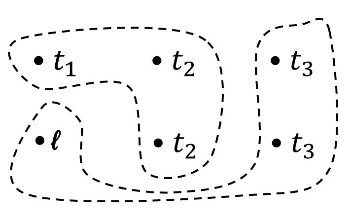
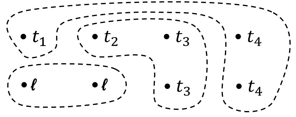
Figure 8: Left: indecomposable partition of $\mathrm{cum}(\widecheck{\mu}_{i},\widecheck{c}_{j_{1}},\widecheck{c}_{j_{2}})$. Right: indecomposable partition of $\mathrm{cum}(\widecheck{\mu}_{i_{1}},\widecheck{\mu}_{i_{2}},\widecheck{c}_{j_{1}},\widecheck{c}_{j_{2}})$

Similarly, for (A.31), when $m=4$, $\mathrm{cum}(\widecheck{\mu}_{i_{1}},\widecheck{\mu}_{i_{2}},\widecheck{c}_{j_{1}},\widecheck{c}_{j_{2}})$ contains an indecomposable partition (see right panel of Figure 8)

$$n^{-4}\sum_{t_{1},t_{2},t_{3},t_{4}}|\mathrm{cum}(X_{t_{1}},X_{t_{4}},X_{t_{4}+j_{2}})\mathrm{cum}(X_{t_{2}},X_{t_{3}},X_{t_{3}+j_{1}})\mathrm{cum}(X_{i_{1}},X_{i_{2}})|$$

$$\leq Cn^{-4}\left(\sum_{t_{1},t_{4}=1}^{n}|\kappa_{3}(t_{4}-t_{1},t_{4}-t_{1}+j_{2})|\right)\left(\sum_{t_{2},t_{3}=1}^{n}|\kappa_{3}(t_{3}-t_{2},t_{3}-t_{2}+j_{1})|\right)=O(n^{-2}).$$

thus loses an order of two. Proof for (A.28) and (A.31) in a general case uses a similar induction argument from the above but we omit the proof. $\Box$

We now need to prove that the derivative of the random function $g(\cdot)$ defined in Theorem 2.3, equation (A.15) is bounded in probability. We recall these bounds are required to show that the final term in the Taylor expansion of $\widehat{J}_{n}(\omega;f_{p})-\widehat{J}_{n}(\omega;f_{p})$ with respect to $\{c_{j}\}_{j=0}^{p}$ is bounded in probability.

To do so, we define the following notation. Let $\underline{\widetilde{c}}_{p}=(\widetilde{c}_{0},\widetilde{c}_{1},\ldots,\widetilde{c}_{p})^{\prime}$ be a random vector such that $\widetilde{\underline{c}}_{p}$ is a convex combination of the true covariance vector $\underline{c}_{p}=(c_{0},\ldots,c_{p})^{\prime}$ and the sample covariance vector $\underline{\widehat{c}}_{p}=(\widehat{c}_{0,n},\ldots,\widehat{c}_{p,n})^{\prime}$. Thus $\widetilde{c}_{s}$ is also a sample covariance that inherits many of the properties of the original sample covariance $\widehat{c}_{s,n}$. Based on these definitions we define the matrix and vector $\widetilde{R}_{p,n}$and $\underline{\widetilde{r}}_{p,n}$ where $(\widetilde{R}_{p,n})_{s,t}=\widetilde{c}_{s-t}$ and $(\underline{\widetilde{r}}_{p,n})_{s}=\widetilde{c}_{s}$. As our aim is to bound the derivatives in the proof Theorem 2.3, using (A.15) and (A.16) we define the random function

$$g_{\ell,p}(\omega,\widetilde{\underline{c}}_{p,n})=\frac{\underline{\widetilde{r}}_{p,n}^{\prime}\widetilde{R}_{p,n}^{-1}\underline{e}_{\ell}(\omega)}{1-\underline{\widetilde{r}}_{p}^{\prime}\widetilde{R}_{p,n}^{-1}\underline{e}_{0}(\omega)}=\frac{\widetilde{a}_{\ell,p}(\omega)}{1-\widetilde{a}_{0,p}(\omega)}$$ (A.33)

where

$$\widetilde{a}_{\ell,p}(\omega)=\sum_{s=0}^{p-\ell}\widetilde{a}_{\ell+s,n}e^{-is\omega},\quad a_{0}\equiv 0,$$

$\underline{\widetilde{a}}_{p,n}=\widetilde{R}_{p,n}^{-1}\underline{\widetilde{r}}_{p,n}$ and $\underline{e}_{\ell}(\omega)$ is defined in (A.17). In the following lemma we show that the derivatives of $g_{\ell,p}(\omega,\widetilde{\underline{c}}_{p,n})$ are uniformly bounded in probability.

Lemma A.2

Suppose Assumptions 2.1 and 2.2 hold with $m=2$. For $1\leq\ell\leq p$, let $g_{\ell,p}(\omega,\widetilde{\underline{c}}_{p})$ be defined as in (A.33), where we recall $\widetilde{\underline{c}}_{p}$ denote a convex combination of the true covariances $\underline{c}_{p}=(c_{0},\ldots,c_{p})^{\prime}$ and the sample autocovariances $\widehat{\underline{c}}_{p}=(\widehat{c}_{0,n},\ldots,\widehat{c}_{p,n})^{\prime}$.

If $p^{3/2}n^{-1/2}\rightarrow 0$ as $p,n\rightarrow\infty$, then for $k\in\mathbb{N}^{+}$ we have

$$\sup_{\omega}\sup_{1\leq\ell\leq p}\sup_{0\leq j_{1},...,j_{k}\leq p}\left|\frac{\partial^{k}g_{\ell,p}(\omega,\widetilde{\underline{c}}_{p})}{\partial\widetilde{c}_{j_{1}}\cdots\partial\widetilde{c}_{j_{k}}}\right|=O_{p}(1).$$

PROOF. First some simple preliminary comments are in order. We observe that $\widetilde{a}_{\ell,p}(\omega)$ is a linear function of $\widetilde{\underline{a}}_{p}=(\widetilde{a}_{1,p},...,\widetilde{a}_{p,p})^{\prime}$ and $\widetilde{\underline{a}}_{p}=\widetilde{R}_{p}^{-1}\widetilde{\underline{r}}_{p}$. Therefore

$$g_{\ell,p}(\omega,\widetilde{\underline{c}}_{p,n})=\frac{\underline{\widetilde{r}}_{p,n}^{\prime}\widetilde{R}_{p,n}^{-1}\underline{e}_{\ell}(\omega)}{1-\underline{\widetilde{r}}_{p}^{\prime}\widetilde{R}_{p,n}^{-1}\underline{e}_{0}(\omega)}=\frac{\widetilde{a}_{\ell,p}(\omega)}{1-\widetilde{a}_{0,p}(\omega)}$$

is an analytic function of $\widetilde{\underline{c}}_{p}$, thus for all $k$ we can evaluate its $k$ order partial derivative.

Since $g_{\ell,p}(\omega,\widetilde{\underline{c}}_{p,n})$ is a function of $\widetilde{\underline{a}}_{p}$ we require some consistency results on $\widetilde{\underline{a}}_{p}$. By Lemma A.1 (here we use Assumptions 2.1(ii) and 2.2), it is easy to show $\sup_{s}\mathbb{E}[\widehat{c}_{s,n}-c_{s}]^{2}=O(n^{-1/2})$ and $\widetilde{c}_{s}$ is a convex combination of $\widehat{c}_{s,n}$ and $c_{s}$, then $\sup_{s}\mathbb{E}[\widetilde{c}_{s}-c_{s}]^{2}=O(n^{-1/2})$. Thus since $\widetilde{\underline{a}}_{p}=\widetilde{R}_{p}^{-1}\widetilde{\underline{r}}_{p}$ we have

$$\left|\underline{\widetilde{a}}_{p}-\underline{a}_{p}\right|_{1}=O_{p}(pn^{-1/2}).$$ (A.34)

where $|\cdot|_{p}$ is an $\ell_{p}$-norm. With this in hand, we can prove that the derivatives of $g_{\ell,p}(\omega,\widetilde{\underline{c}}_{p})$ are uniformly bounded in probability. We give the precise details below.

In order to prove the result, we first consider the first derivative of $g_{\ell,p}(\omega,\widetilde{\underline{c}}_{p,n})$. By the chain rule, we have

$$\frac{\partial g_{\ell,p}}{\partial\widetilde{c}_{j}}=\sum_{r=1}^{p}\frac{\partial g_{\ell,p}}{\partial\widetilde{a}_{r,p}}\frac{\partial\widetilde{a}_{r,p}}{\partial\widetilde{c}_{j}}$$ (A.35)

where basic algebra gives

$$\frac{\partial g_{\ell,p}}{\partial\widetilde{a}_{r,p}}=\frac{e^{-ir\omega}}{(1-\widetilde{a}_{0,p}(\omega))^{2}}\times\left\{\begin{array}[]{ll}\widetilde{a}_{\ell,p}(\omega)&r<\ell\\ e^{i\ell\omega}(1-\sum_{s=1}^{\ell-1}\widetilde{a}_{s,p}e^{-is\omega})&r\geq\ell\end{array}\right.$$ (A.38)

and

$$\left(\frac{\partial\widetilde{a}_{1,p}}{\partial\widetilde{c}_{j}},\ldots,\frac{\partial\widetilde{a}_{p,p}}{\partial\widetilde{c}_{j}}\right)^{\prime}=\frac{\partial\widetilde{\underline{a}}_{p}}{\partial\widetilde{c}_{j}}=\frac{\partial}{\partial\widetilde{c}_{j}}\widetilde{R}_{p}^{-1}\widetilde{\underline{r}}_{p}=\widetilde{R}^{-1}_{p}\left(\frac{\partial\widetilde{R}_{p}}{\partial\widetilde{c}_{j}}\right)\widetilde{\underline{a}}_{p}+\widetilde{R}_{p}^{-1}\frac{\partial\widetilde{\underline{r}}_{p}}{\partial\widetilde{c}_{j}}.$$ (A.39)

Therefore to bound (A.35) we take its absolute. We will bound the left hand side of an inequality below

$$\left|\frac{\partial g_{\ell,p}}{\partial\widetilde{c}_{j}}\right|\leq\sup_{\omega,s,\ell}\left|\frac{\partial g_{\ell,p}}{\partial\widetilde{a}_{s,p}}\right|\sum_{r=1}^{p}\left|\frac{\partial\widetilde{a}_{r,p}}{\partial\widetilde{c}_{j}}\right|,$$ (A.40)

which will prove the result for the first derivative. Therefore, we bound each term:
$\sup_{\omega,s,\ell}\left|\partial g_{\ell,p}/\partial\widetilde{a}_{s,p}\right|$ and $(\partial\widetilde{a}_{1,p}/\partial\widetilde{c}_{j},\ldots,\partial\widetilde{a}_{p,p}/\partial\widetilde{c}_{j})$.

A bound for $\sup_{\omega,s,\ell}|\partial g_{\ell,p}/\partial\widetilde{a}_{s,p}|$    Using (A.38) gives

$$\sup_{1\leq\ell,r\leq p}\sup_{\omega}\left|\frac{\partial g_{\ell,p}(\omega,\widetilde{c})}{\partial\widetilde{a}_{r,p}}\right| \leq \sup_{\omega}\sup_{1\leq\ell\leq p}\frac{1}{|1-\sum_{s=1}^{p}\widetilde{a}_{s,p}e^{-is\omega}|^{2}}\left(\sum_{s=0}^{p-\ell}\left|\widetilde{a}_{s+\ell,p}e^{-is\omega}\right|+|1-\sum_{s=1}^{p}\widetilde{a}_{s,p}e^{-is\omega}|\right)$$ (A.41)

$$\leq \sup_{\omega}\frac{1}{|1-\sum_{s=1}^{p}\widetilde{a}_{s,p}e^{-is\omega}|^{2}}\left(1+2\sum_{s=1}^{p}|\widetilde{a}_{s,p}|\right).$$

We first bound the denominator of the above. It is clear that

$$\inf_{\omega}|1-\sum_{s=1}^{p}\widetilde{a}_{s,p}e^{-is\omega}| \geq \inf_{\omega}\left(|1-\sum_{s=1}^{p}a_{s,p}e^{-is\omega}|-|\sum_{s=1}^{p}(a_{s,p}-\widetilde{a}_{s,p})e^{-is\omega}|\right)$$

$$\geq \inf_{\omega}\left(|1-\sum_{s=1}^{p}a_{s,p}e^{-is\omega}|-\sum_{s=1}^{p}|a_{s,p}-\widetilde{a}_{s,p}|\right).$$

By using (A.34), we have $|\underline{a}_{p}-\underline{\widetilde{a}}_{p}|_{1}=O_{p}(pn^{-1/2})$ thus for $pn^{-1/2}\rightarrow 0$, we have that $\sum_{s=1}^{p}|a_{s,p}-\widetilde{a}_{s,p}|=o_{p}(1)$. Moreover, by Assumption 2.1(i) (and the Baxter’s inequality), the first term is bounded away from 0 for large $p$. Therefore, we conclude that $\inf_{\omega}|1-\sum_{s=1}^{p}\widetilde{a}_{s,p}e^{-is\omega}|$ is bounded away in probability from zero, thus giving

$$\frac{1}{|1-\sum_{s=1}^{p}\widetilde{a}_{s,p}e^{-is\omega}|^{2}}=O_{p}(1)$$ (A.42)

as $n,p\rightarrow\infty$ and $pn^{-1/2}\rightarrow 0$. This bounds the denominator of (A.41). Next to bound the numerator in (A.41) we use again (A.34)

$$\sum_{s=1}^{p}|\widetilde{a}_{s,p}|\leq\sum_{s=1}^{p}|a_{s,p}|+\sum_{s=1}^{p}|\widetilde{a}_{s,p}-a_{s,p}|=O_{p}(1+pn^{-1/2}).$$ (A.43)

Therefore, by (A.42) and (A.43) we have

$$\sup_{\omega}\sup_{1\leq\ell\leq p}\sup_{1\leq k\leq p}\left|\frac{\partial g_{\ell,p}(\omega,\widetilde{c})}{\partial\widetilde{a}_{k,p}}\right|=O_{p}(1).$$ (A.44)

A bound for $(\partial\widetilde{a}_{1,p}/\partial\widetilde{c}_{j},\ldots,\partial\widetilde{a}_{p,p}/\partial\widetilde{c}_{j})$ We use the expansion in (A.39):

$$\left(\frac{\partial a_{1,p}}{\partial c_{j}},\ldots,\frac{\partial a_{p,p}}{\partial c_{j}}\right)^{\prime}=\frac{\partial\underline{a}_{p}}{\partial c_{j}}=\frac{\partial}{\partial c_{j}}R^{-1}\underline{r}_{p}=R^{-1}_{p}\left(\frac{\partial R_{p}}{\partial c_{j}}\right)\underline{a}_{p}+R_{p}^{-1}\frac{\partial\underline{r}_{p}}{\partial c_{j}}.$$

We observe that the structure of Toeplitz matrix of $R_{p}$ means that $\partial R_{p}/\partial c_{j}$ has ones on the lower and upper $j$th diagonal and is zero elsewhere and $\partial\widetilde{\underline{r}}_{p}/\partial c_{j}$ is one at the $j$th entry and zero elsewhere. Using these properties we have

$$\sup_{0\leq j\leq p}\left|\frac{\partial R_{p}}{\partial c_{j}}\underline{a}_{p}\right|_{1}\leq 2\sum_{s=1}^{p}|a_{s,p}|\quad\text{and}\quad\sup_{0\leq j\leq p}\left|R_{p}^{-1}\frac{\partial\underline{r}_{p}}{\partial c_{j}}\right|_{1}\leq\|R_{p}^{-1}\|_{1}$$

where $\|A\|_{p}$ is an operator norm induced by the vector $\ell_{p}$-norm. Therefore, using the above and the inequality $|A\underline{x}|_{1}\leq\|A\|_{1}|\underline{x}|_{1}$ gives

$$\sup_{0\leq j\leq p}\sum_{s=1}^{p}\left|\frac{\partial\widetilde{a}_{s,p}}{\partial\widetilde{c}_{j}}\right| \leq \left|\widetilde{R}_{p}^{-1}\frac{\partial\widetilde{R}_{p}}{\partial\widetilde{c}_{j}}\underline{\widetilde{a}}_{p}\right|_{1}+\left|\widetilde{R}^{-1}_{p}\frac{\partial\widetilde{\underline{r}}_{p}}{\partial\widetilde{c}_{j}}\right|_{1}$$ (A.45)

$$\leq 2\|\widetilde{R}^{-1}_{p}\|_{1}\sum_{s=1}^{p}|\widetilde{a}_{s,p}|+\|\widetilde{R}_{p}^{-1}\|_{1}\leq\|\widetilde{R}^{-1}_{p}\|_{1}\left(2\sum_{s=1}^{p}|\widetilde{a}_{s,p}|+1\right),$$

where we note that in (A.43) we have shown that $\sum_{s=1}^{p}|\widetilde{a}_{s,p}|=O_{p}(1+pn^{-1/2})$. Next we show $\|\widetilde{R}_{p}^{-1}\|_{1}=O_{p}(1)$. To do this we define the circulant matrix $C_{p}(f^{-1})$ where

$$(C_{p}(f^{-1}))_{u,v}=n^{-1}\sum_{k=1}^{p}f^{-1}\left(\frac{2\pi k}{p}\right)\exp{\left(-i(u-v)\frac{2\pi k}{p}\right)}=\sum_{r\in\mathbb{Z}}K_{f^{-1}}(u-v+rp)$$

with $K_{f^{-1}}(r)=(2\pi)^{-1}\int_{0}^{2\pi}f^{-1}(\omega)e^{-ir\omega}d\omega$. By using Theorem 3.2 in SY20,

$$\|R_{p}^{-1}\|_{1} \leq \|C_{p}(f^{-1})\|_{1}+\|R_{p}^{-1}-C_{p}(f^{-1})\|_{1}\leq\|C_{p}(f^{-1})\|_{1}+A(f)$$

where $A(f)$ is a finite constant that does not depend on $p$ (the exact form is given in SY20). Furthermore we have

$$\|C_{p}(f^{-1})\|_{1}=\max_{1\leq v\leq p}\sum_{u=1}^{p}|C_{p}(f^{-1})_{u,v}|\leq\max_{1\leq v\leq p}\sum_{u=1}^{p}\sum_{r\in\mathbb{Z}}|K_{f^{-1}}(u-v+rp)|=\sum_{r\in\mathbb{Z}}|K_{f^{-1}}(r)|<\infty.$$

altogether this gives $\|R_{p}^{-1}\|_{1}=O(1)$. To bound the random matrix $\|\widetilde{R}_{p}^{-1}\|_{1}$ we use that

$$\|\widetilde{R}_{p}^{-1}\|_{1}\leq\|R_{p}^{-1}\|_{1}+\|\widetilde{R}_{p}^{-1}-R_{p}^{-1}\|_{1}\leq\|R_{p}^{-1}\|_{1}+\sqrt{p}\|\widetilde{R}_{p}^{-1}-R_{p}^{-1}\|_{2}.$$

By using similar argument to Corollary 1 in McMurry and Politis [2015], we have $\|\widetilde{R}_{p}^{-1}-R_{p}^{-1}\|_{2}=O(pn^{-1/2})$. Thus, if $p^{3/2}n^{-1/2}\rightarrow 0$ as $p$ and $n\rightarrow\infty$, then $\|\widetilde{R}_{p}^{-1}\|_{1}=O_{p}(1)$. Substituting this into (A.45) gives

$$\sup_{0\leq j\leq p}\sum_{s=1}^{p}\left|\frac{\partial\widetilde{a}_{s,p}}{\partial\widetilde{c}_{j}}\right| \leq \|\widetilde{R}^{-1}_{p}\|_{1}\left(2\sum_{s=1}^{p}|\widetilde{a}_{s,p}|+1\right)=O_{p}(1).$$ (A.46)

$\bullet$ Bound for the first derivatives Substituting the two bounds above into (A.40), gives the bound for the first derivative:

$$\sup_{\omega}\left|\frac{\partial g_{\ell,p}(\omega,\widetilde{\underline{c}}_{p})}{\partial\widetilde{c}_{j}}\right|\leq\sup_{\omega}\sup_{1\leq\ell\leq p}\sup_{1\leq k\leq p}\left|\frac{\partial g_{\ell,p}(\omega,\widetilde{c}_{p})}{\partial\widetilde{a}_{k,p}}\right|\|\widetilde{R}_{p}^{-1}\|_{1}\left(2\sum_{s=1}^{p}|\widetilde{a}_{s,p}|+1\right)=O_{p}\left(1\right).$$

$\bullet$ Bound for the second derivatives To simplify notation, we drop the subscript $p$ in $a_{k,p}$ (though we should keep in mind it is a function of $p$). Using the chain rule we have

$$\frac{\partial^{2}g_{\ell,p}}{\partial c_{i}\partial c_{j}}=\sum_{r=1}^{p}\frac{\partial g_{\ell,p}}{\partial a_{r}}\cdot\frac{\partial^{2}a_{r}}{\partial c_{i}\partial c_{j}}+\sum_{r_{1},r_{2}=1}^{p}\frac{\partial^{2}g_{\ell,p}}{\partial a_{r_{1}}\partial a_{r_{2}}}\cdot\frac{\partial a_{r_{1}}}{\partial c_{i}}\cdot\frac{\partial a_{r_{2}}}{\partial c_{j}}.$$

Thus taking absolute of the above gives

$$\left|\frac{\partial^{2}g_{\ell,p}}{\partial c_{i}\partial c_{j}}\right|\leq\sup_{k,\omega}\left|\frac{\partial g_{\ell,p}}{\partial a_{k}}\right|\sum_{k=1}^{p}\left|\frac{\partial^{2}a_{k}}{\partial c_{i}\partial c_{j}}\right|+\sup_{r_{1},r_{2},\omega}\left|\frac{\partial^{2}g_{\ell,p}}{\partial a_{r_{1}}\partial a_{r_{2}}}\right|\left(\sum_{r=1}^{p}\left|\frac{\partial a_{r}}{\partial c_{i}}\right|\right)^{2}.$$ (A.47)

We now bound the terms in (A.47). We first consider the term $\partial^{2}g_{\ell,p}/\partial a_{k}\partial a_{t}$, which by using (A.38) is

$$\frac{\partial^{2}g_{\ell,p}}{\partial a_{k}\partial a_{t}}=\frac{e^{-i(k+t)\omega}}{(1-a_{0,p}(\omega))^{3}}\times\left\{\begin{array}[]{ll}a_{\ell,p}(\omega)&k,t<\ell\\ e^{i\ell\omega}(1-\sum_{s=1}^{\ell-1}a_{s}e^{-is\omega})+a_{\ell,p}(\omega)&k<\ell\leq t\\ e^{i\ell\omega}(1-\sum_{s=1}^{\ell-1}a_{s}e^{-is\omega})&k,t\geq\ell\\ \end{array}\right.$$

Therefore, using a similar argument as used to bound (A.44), we have

$$\sup_{\omega}\sup_{1\leq\ell,k,t\leq p}\left|\frac{\partial^{2}g_{\ell,p}(\omega,\underline{\widetilde{c}}_{p})}{\partial\widetilde{a}_{k}\partial\widetilde{a}_{t}}\right|=O_{p}(1)$$ (A.49)

with $pn^{-1/2}\rightarrow 0$ as $p\rightarrow\infty$ and $n\rightarrow\infty$

Next, we obtain a probabilistic bound for $|\partial^{2}\widetilde{\underline{a}}/\partial\widetilde{c}_{i}\partial\widetilde{c}_{j}|_{1}$. Note that by (A.39)

$$\frac{\partial^{2}\underline{a}_{p}}{\partial c_{i}\partial c_{j}} = R_{p}^{-1}\left(\frac{\partial R_{p}}{\partial c_{i}}\right)R_{p}^{-1}\left(\frac{\partial R_{p}}{\partial c_{j}}\right)\underline{a}_{p}+R_{p}^{-1}\left(\frac{\partial R_{p}}{\partial c_{i}}\right)R_{p}^{-1}\frac{\partial\underline{r}_{p}}{\partial c_{j}}$$

$$+R_{p}^{-1}\left(\frac{\partial R_{p}}{\partial c_{j}}\right)R_{p}^{-1}\left(\frac{\partial R_{p}}{\partial c_{i}}\right)\underline{a}_{p}+R_{p}^{-1}\left(\frac{\partial R_{p}}{\partial c_{j}}\right)R_{p}^{-1}\frac{\partial\underline{r}_{p}}{\partial c_{i}}$$

$$= R_{p}^{-1}\left(\frac{\partial R_{p}}{\partial c_{i}}\right)\frac{\partial\underline{a}_{p}}{\partial c_{j}}+R_{p}^{-1}\left(\frac{\partial R_{p}}{\partial c_{j}}\right)\frac{\partial\underline{a}_{p}}{\partial c_{i}}.$$

Our focus will be on the first term of right hand side of the above. By symmetry, bound for the second term is the same. Using the submultiplicative of the operator norm we have

$$\left|R_{p}^{-1}\left(\frac{\partial R_{p}}{\partial c_{i}}\right)\frac{\partial\underline{a}_{p}}{\partial c_{j}}\right|_{1}\leq\|R_{p}^{-1}\left(\frac{\partial R_{p}}{\partial c_{i}}\right)\|_{1}\left|\frac{\partial\underline{a}_{p}}{\partial c_{j}}\right|_{1}\leq\|R_{p}^{-1}\|_{1}\|\frac{\partial R_{p}}{\partial c_{i}}\|_{1}\left|\frac{\partial\underline{a}_{p}}{\partial c_{j}}\right|_{1}\leq 2\|R_{p}^{-1}\|_{1}\left|\frac{\partial\underline{a}_{p}}{\partial c_{j}}\right|_{1}.$$

Therefore by (A.46),

$$\sup_{0\leq i,j\leq p}\left|\frac{\partial^{2}\underline{\widetilde{a}}_{p}}{\partial\widetilde{c}_{i}\partial\widetilde{c}_{j}}\right|_{1}\leq 4\|\widetilde{R}_{p}^{-1}\|_{1}\sup_{0\leq j\leq p}\left|\frac{\partial\underline{\widetilde{a}}_{p}}{\partial\widetilde{c}_{j}}\right|_{1}=O_{p}\left(1\right).$$ (A.50)

The bounds in (A.49) and (A.50) gives bounds for two of the terms in (A.47). The remaining two terms in (A.47) involve only first derivatives and bounds for these terms are given in equations (A.44) and (A.46). Thus by using (A.47) and the four bounds described above we have

$$\sup_{\omega}\sup_{1\leq\ell\leq p}\sup_{0\leq j_{1},j_{2}\leq p}\left|\frac{\partial^{2}g_{\ell,p}}{\partial\widetilde{c}_{j_{1}}\partial\widetilde{c}_{j_{2}}}(\omega,\underline{\widetilde{c}}_{p,n})\right|=O_{p}(1),$$

which gives a bound for the second derivative.

$\bullet$ Bounds for the higher order derivatives The bounds for the higher order derivatives follows a similar pattern. We bound the $m$th order derivatives

$$\frac{\partial^{m}g_{\ell,p}}{\partial\widetilde{a}_{t_{1}}\partial\widetilde{a}_{t_{2}}\ldots\partial\widetilde{a}_{t_{m}}}\quad\textrm{and}\quad\frac{\partial^{m}\widetilde{\underline{a}}_{p}}{\partial\widetilde{c}_{i_{1}}\partial\widetilde{c}_{i_{1}}\ldots\partial\widetilde{c}_{i_{m}}},$$

using the methods described above. In particular, we can show that

$$\left|\frac{\partial^{m}g_{\ell,p}}{\partial\widetilde{a}_{t_{1}}\partial\widetilde{a}_{t_{2}}\ldots\partial\widetilde{a}_{t_{m}}}\right|=O_{p}(1)\quad\textrm{and}\quad\left|\frac{\partial^{m}\widetilde{\underline{a}}}{\partial\widetilde{c}_{j_{1}}\partial\widetilde{c}_{j_{1}}\ldots\partial\widetilde{c}_{j_{m}}}\right|=O_{p}(1).$$

Since these bounds hold for $1\leq m\leq k$, by using the chain rule we have

$$\sup_{\omega}\sup_{1\leq\ell\leq p}\sup_{0\leq j_{1},\ldots,j_{k}\leq p}\left|\frac{\partial^{k}g_{\ell,p}}{\partial\widetilde{c}_{j_{1}}\partial\widetilde{c}_{j_{2}}\ldots\partial\widetilde{c}_{j_{k}}}(\omega,\underline{\widetilde{c}}_{p})\right|=O_{p}(1).$$

This proves the lemma. $\Box$

Appendix B Additional simulations and data analysis

B.1 The autocorrelation estimator

In this section, we estimate the autocorrelation function (ACF) using the integrated periodogram estimator in Section 3. Recall that we estimate the autocovariances using

$$\breve{c}_{n}(r)=\frac{1}{2\pi}\int_{0}^{2\pi}cos(r\omega)\widetilde{I}_{n}(\omega)d\omega$$ (B.1)

where $\widetilde{I}_{n}(\cdot)$ is one of the periodograms in Section 4. Based on $\breve{c}_{n}(r)$, the natural estimator of the ACF at lag $r$ is

$$\breve{\rho}_{n}(r)=\frac{\breve{c}_{n}(r)}{\breve{c}_{n}(0)}.$$

Note that if $\widetilde{I}_{n}(\cdot)$ is the regular periodogram, $\breve{c}_{n}(\cdot)$ and $\breve{\rho}_{n}(\cdot)$ become the classical sample autocovariances and sample ACFs respectively.

We generate the Gaussian time series from (M1) and (M2) in Section 4 and evaluate the ACF estimators at lag $r=0,1,...,10$. For the computational purpose, we approximate (B.1) using Reimann sum over 500 uniform partitions on $[0,2\pi]$.

Figures 9$-$11 show the average (left panels), bias (middle panels), and the mean squared error (MSE; right panels) of the ACF estimators at each lag for different models and sample sizes. Analogous to the results in Section 4.1, we observe that the complete and complete tapered periodogram significantly reduce the bias as compared to the regular (black) and tapered (blue) periodogram for all the models.

The MSE paints a complex picture. From the left panels in Figures 9$-$11 for (M1), we observe when the lag $r$ is odd, the true $\rho(r)=0$. For these lags, all the ACF estimators are almost unbiased, and the variance dominates. This is why we observe the oscillation the MSE in (M1) over $r$. For (M2), the bias of all estimators are very small even for an extremely small sample size $n$=20, and thus the variance dominates. For the small sample sizes ($n$=20 and 50), MSE of the complete periodograms is larger then the classical methods (Regular and tapered). Whereas for the large sample size ($n$=300), it seems that the tapering increases the MSE.

Figure 9: ACF: The average (left), bias (middle), and MSE (right) of the ACF estimators at lag $r=0,...,10$. The length of the time series $n=20$.

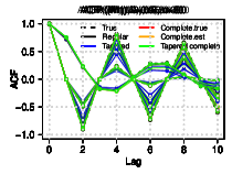
Figure 10: ACF: Same as Figure 9 but for $n=50$.

Figure 11: ACF: Same as Figure 9 but for $n=300$.

To assess the overall performance of the ACF estimators, we evaluate the averaged mean squared error (MSE) and squared bias (BIAS)

$$\text{MSE}=\frac{1}{10B}\sum_{r=1}^{10}\sum_{j=1}^{B}(\breve{\rho}^{(j)}_{n}(r)-\rho(r))^{2},\quad\text{BIAS}=\frac{1}{10}\sum_{r=1}^{10}\left(B^{-1}\sum_{j=1}^{B}\breve{\rho}^{(j)}_{n}(r)-\rho(r)\right)^{2}$$

where $\breve{\rho}^{(j)}$ is the $j$th replication of one of the ACF estimators. The results are summarized in Table 3. As described above, our method has a marked gain in the BIAS compared to the classical ACF estimators for all models. Moreover, the MSE is comparable, at least for our models, and even has a smaller MSE when the sample size is small and/or there is a strong dependent in the lags.

Model	$n$	metric	Regular	Tapered	Complete(True)	Complete(Est)	Tapered complete
(M1), $\lambda=0.7$	20	MSE	$0.038$	$0.040$	$0.038$	$0.044$	$0.046$
		BIAS	$0.002$	$0.002$	$0$	$0.001$	$0.001$
	50	MSE	$0.021$	$0.023$	$0.021$	$0.022$	$0.024$
		BIAS	$0$	$0$	$0$	$0$	$0$
	300	MSE	$0.004$	$0.005$	$0.004$	$0.004$	$0.004$
		BIAS	$0$	$0$	$0$	$0$	$0$
(M1), $\lambda=0.9$	20	MSE	$0.061$	$0.064$	$0.045$	$0.062$	$0.063$
		BIAS	$0.023$	$0.025$	$0.003$	$0.008$	$0.008$
	50	MSE	$0.030$	$0.032$	$0.025$	$0.029$	$0.030$
		BIAS	$0.005$	$0.005$	$0.001$	$0.002$	$0.002$
	300	MSE	$0.005$	$0.006$	$0.005$	$0.005$	$0.005$
		BIAS	$0$	$0$	$0$	$0$	$0$
(M1), $\lambda=0.95$	20	MSE	$0.077$	$0.082$	$0.039$	$0.063$	$0.064$
		BIAS	$0.045$	$0.049$	$0.004$	$0.015$	$0.014$
	50	MSE	$0.032$	$0.034$	$0.022$	$0.027$	$0.028$
		BIAS	$0.011$	$0.011$	$0.002$	$0.003$	$0.003$
	300	MSE	$0.005$	$0.005$	$0.004$	$0.004$	$0.004$
		BIAS	$0$	$0$	$0$	$0$	$0$
(M2)	20	MSE	$0.062$	$0.065$	$-$	$0.074$	$0.077$
		BIAS	$0.006$	$0.006$	$-$	$0.002$	$0.002$
	50	MSE	$0.036$	$0.040$	$-$	$0.040$	$0.042$
		BIAS	$0.001$	$0.001$	$-$	$0$	$0$
	300	MSE	$0.008$	$0.009$	$-$	$0.008$	$0.008$
		BIAS	$0$	$0$	$-$	$0$	$0$

Table 3: MSE and BIAS of an ACF estimators.

B.2 Analysis of sunspot data

We conclude by returning to the sunspot data which first motivated Schuster to define the periodogram 120 years ago.

Sunspots are visibly darker areas that are apparent on the surface of the Sun that are captured from satellite imagery or man-made orbiting telescopes. The darker appearance of these areas is due to their relatively cooler temperatures compared to other parts of the Sun that are attributed to the relatively stronger magnetic fields.

There is a rich history of analysis of the sunspot data and probably Schuster (1897, 1906) is the first one who analyzed this data in a frequency domain. Schuster developed the “periodogram” to study periodicities in sunspot activity. As mentioned in the introduction the Sunspot data has since served as a benchmark for developing several theories and methodologies and theories related to spectral analysis of time series. A broader account of these analyses can be found in Chapter 6$-$8 of Bloomfield [2004] and references therein.

In this section we implement the four comparator periodograms in Section 4 to estimate and corroborate the spectrum of the sunspot data. The dataset we have used is a subset of the data available at the World Data Center Sunspot Index and Long-term Solar Observations (WDC-SILSO), Royal Observatory of Belgium, Brussels (http://sidc.be/silso/). We use length $n$=3168 total monthly count of sunspots from Jan 1749 to Dec 2013. All periodograms are computed after removing the sample mean from the data. Figure 12 shows the time series plot (right), four different periodograms (middle) and smoothed periodograms (right). We smooth the periodogram using the Bartlett window function from Section 4.2 with the bandwidth $m=5$ ($\approx n^{1/5}$).

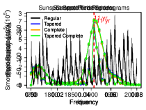
Figure 12: Right: Monthly Sunspot time series plot of length 3168 (264 years) starting from Jan 1749. Middle: Trajectories of the four different periodograms; regular, regular tapered, complete and tapered complete periodogram. left: Smoothed periodograms using Bartlett window.

From the middle panel of Figure 12, we observe that all the periodograms detect the peak corresponding to maximum sunspot activity at the 11-year cycle. The peak at the 11-year cycle (frequency $0.046$) for the complete periodogram (orange) is the largest, at about $7.1\times 10^{5}$, the regular (black) and complete tapered(green) periodogram is slightly lower at about $6.98\times 10^{5}$. Whereas, the tapered periodogram (blue) is the lowest at about $6.25\times 10^{5}$. Looking at in the neighbourhood of the main peak, we observe that there is very little difference between all the periodograms. This suggests that these “side peaks” in the neighbourhood of $0.046$ are not an artifact of the periodogram but a feature of the data. Which further suggests that the sunspot data does not contain a fixed period but a quasi-dominant period in the frequencies range $0.042-0.058$ ($9.1-12.6$ years). The effect is clearer after smoothing the periodogram (right panel of Figure 12). Smoothing the complete and tapered complete periodogram yields a more dominant peak at $0.046$ ($11$ years), but the quasi-frequency band remains. Further, a secondary dominate frequency is seen in the very low frequency around $0.006$ ($88$ years) which is more pronounced when the smoothing is done using the (regular) tapered periodogram and tapered complete periodogam. In summary, due to the large sample size all the different periodograms exhibit very similar behaviour. However, even within the large sample setting (where theoretically all the periodograms are asymptotically equivalent) the complete periodograms appear to better capture the amplitude of the peak.

References

Bardet et al. [2008]
J.-M. Bardet, P. Doukhan, and J. R. León.
Uniform limit theorems for the integrated periodogram of weakly
dependent time series and their applications to Whittle’s estimate.
J. Time Series Anal., 29(5):906–945,
2008.
Bartlett [1953]
M. S. Bartlett.
Approximate confidence intervals II.
Biometrika, 40:306–317, 1953.
Baxter [1962]
G. Baxter.
An asymptotic result for the finite predictor.
Math. Scand., 10:137–144, 1962.
Beltrão and Bloomfield [1987]
K. I. Beltrão and P. Bloomfield.
Determining the bandwidth of a kernel spectrum estimate.
J. Time Series Anal., 8(1):21–38, 1987.
Bhansali [1996]
R. J. Bhansali.
Asymptotically efficient autoregressive model selection for multistep
prediction.
Ann. Inst. Statist. Math., 48(3):577–602,
1996.
Bloomfield [2004]
Peter Bloomfield.
Fourier analysis of time series: an introduction.
John Wiley & Sons, 2004.
Brillinger and Rosenblatt [1967]
D. R. Brillinger and M. Rosenblatt.
Asymptotic theory of estimates of th-order spectra.
Proc. Natl. Acad. Sci. USA, 57:206–210, 1967.
Brillinger [1981]
David R Brillinger.
Time series: Data Analysis and Theory, volume 36.
SIAM, 1981.
Brockwell and Davis [2006]
Peter J. Brockwell and Richard A. Davis.
Time series: theory and methods.
Springer Series in Statistics. Springer, New York, 2006.
Reprint of the second (1991) edition.
Dahlhaus [1983]
R. Dahlhaus.
Spectral analysis with tapered data.
J. Time Series Anal., 4(3):163–175, 1983.
Dahlhaus [1988]
R. Dahlhaus.
Small sample effects in time series analysis: a new asymptotic theory
and a new estimate.
Ann. Statist., 16(2):808–841, 1988.
Dahlhaus and Janas [1996]
R. Dahlhaus and D. Janas.
A frequency domain bootstrap for ratio statistics in time series
analysis.
Ann. Statist., 24(5):1934–1963, 1996.
Eichler [2008]
M. Eichler.
Testing nonparametric and semi-parametric hypothesis in vector
stationary processes.
J. Multivariate Anal., 99:968–1009, 2008.
Hurvich [1985]
C. M. Hurvich.
Data-driven choice of a spectrum estimate: extending the
applicability of cross-validation methods.
J. Amer. Statist. Assoc., 80(392):933–940, 1985.
Hurvich [1988]
C. M. Hurvich.
A mean squared error criterion for time series data windows.
Biometrika, 75(3):485–490, 1988.
Ing and Wei [2005]
C.-K. Ing and C.-Z. Wei.
Order selection for same-realization predictions in autoregressive
processes.
Ann. Statist., 33(5):2423–2474, 2005.
Kley et al. [2019]
T. Kley, P. Preuß, and P. Fryzlewicz.
Predictive, finite-sample model choice for time series under
stationarity and non-stationarity.
Electron. J. Stat., 13(2):3710–3774,
2019.
Krampe et al. [2018]
J. Krampe, J.-P. Kreiss, and E. Paparoditis.
Estimated Wold representation and spectral-density-driven bootstrap
for time series.
J. R. Stat. Soc. Ser. B. Stat. Methodol., 80(4):703–726, 2018.
Kreiss et al. [2011]
J.-P. Kreiss, E. Paparoditis, and D. N. Politis.
On the range of validity of the autoregressive sieve bootstrap.
Ann. Statist., 39(4):2103–2130, 2011.
McMurry and Politis [2015]
T. L. McMurry and D. N. Politis.
High-dimensional autocovariance matrices and optimal linear
prediction.
Electron. J. Stat., 9(1):753–788, 2015.
Mikosch and Zhao [2015]
T. Mikosch and Y. Zhao.
The integrated periodogram of a dependent extremal event sequence.
Stochastic Process. Appl., 125(8):3126–3169, 2015.
Milhøj [1981]
A. Milhøj.
A test of fit in time series models.
Biometrika, 68:177–187, 1981.
Niebuhr and Kreiss [2014]
T. Niebuhr and J.-P. Kreiss.
Asymptotics for autocovariances and integrated periodograms for
linear processes observed at lower frequencies.
Int. Stat. Rev., 82(1):123–140, 2014.
Ombao et al. [2001]
H. C. Ombao, J. A. Raz, R. L. Strawderman, and R. Von Sachs.
A simple generalised crossvalidation method of span selection for
periodogram smoothing.
Biometrika, 88(4):1186–1192, 2001.
Pourahmadi [1983]
M. Pourahmadi.
Exact factorization of the spectral density and its application to
forecasting and time series analysis.
Comm. Statist. Theory Methods, 12(18):2085–2094, 1983.
Pourahmadi [1984]
M. Pourahmadi.
Taylor expansion of
and some applications.
Amer. Math. Monthly, 91(5):303–307, 1984.
Pourahmadi [2001]
Mohsen Pourahmadi.
Foundations of time series analysis and prediction theory.
Wiley Series in Probability and Statistics: Applied Probability and
Statistics. Wiley-Interscience, New York, 2001.
Priestley [1981]
Maurice B. Priestley.
Spectral Analysis and Time Series.
Academic Press, London, 1981.
Randall and Antoni [2011]
R. B. Randall and J. Antoni.
Rolling element bearing diagnostics—a tutorial.
Mechanical systems and signal processing, 25(2):485–520, 2011.
Rosenblatt [1966]
M. Rosenblatt.
Remarks on higher order spectra.
In Multivariate Analysis (Proc. Internat. Sympos.,
Dayton, Ohio, 1965), pages 383–389. Academic Press, New York, 1966.
Schuster [1897]
A. Schuster.
On lunar and solar periodicities of earthquakes.
Proceedings of the Royal Society of London, 61:455–465, 1897.
Schuster [1906]
A. Schuster.
On the periodicities of sunspots.
Philosophical transactions of the royal society A,
206:69–100, 1906.
Smith and Randall [2015]
W. A. Smith and R. B. Randall.
Rolling element bearing diagnostics using the case western reserve
university data: A benchmark study.
Mechanical Systems and Signal Processing, 64:100–131, 2015.
Subba Rao [2018]
S. Subba Rao.
Orthogonal samples for estimators in time series.
J. Time Series Anal., 39:313–337, 2018.
Subba Rao and Yang [2020]
S. Subba Rao and J. Yang.
Reconciling the Gaussian and Whittle likelihood with an
application to estimation in the frequency domain.
arXiv preprint arXiv:2001.06966, 2020.
Subba Rao and Gabr [1980]
T. Subba Rao and M. M. Gabr.
A test for linearity of stationary time series.
J. Time Series Anal., 1(2):145–158, 1980.
Subba Rao and Gabr [1984]
T. Subba Rao and M. M. Gabr.
An introduction to bispectral analysis and bilinear time series
models, volume 24 of Lecture Notes in Statistics.
Springer-Verlag, New York, 1984.
Tukey [1967]
J. W. Tukey.
An introduction to the calculations of numerical spectrum analysis.
In Spectral Analysis of Time Series (Proc. Advanced
Sem., Madison, Wis., 1966), pages 25–46. John Wiley, New York, 1967.
Whittle [1953]
P. Whittle.
The analysis of multiple stationary time series.
J. R. Stat. Soc. Ser. B. Stat. Methodol., 15:125–139, 1953.
Whittle [1951]
Peter Whittle.
Hypothesis Testing in Time Series Analysis.
Thesis, Uppsala University, 1951.
Wilson [1972]
G. T. Wilson.
The factorization of matricial spectral densities.
SIAM J. Appl. Math., 23:420–426, 1972.
Zhang and Wu [2018]
D. Zhang and W. B. Wu.
Asymptotic theory for estimators of high-order statistics of
stationary processes.
IEEE Trans. Inform. Theory, 64(7):4907–4922, 2018.