Similarity Search for Efficient Active Learning and Search of Rare Concepts

Abstract

Many active learning and search approaches are intractable for large-scale industrial settings with billions of unlabeled examples. Existing approaches search globally for the optimal examples to label, scaling linearly or even quadratically with the unlabeled data. In this paper, we improve the computational efficiency of active learning and search methods by restricting the candidate pool for labeling to the nearest neighbors of the currently labeled set instead of scanning over all of the unlabeled data. We evaluate several selection strategies in this setting on three large-scale computer vision datasets: ImageNet, OpenImages, and a de-identified and aggregated dataset of 10 billion publicly shared images provided by a large internet company. Our approach achieved similar mean average precision and recall as the traditional global approach while reducing the computational cost of selection by up to three orders of magnitude, enabling web-scale active learning.

1 Introduction

Large-scale unlabeled datasets can contain millions or billions of examples covering a wide variety of underlying concepts [10, 53, 46, 37, 29, 44, 1, 30]. Yet, these massive datasets often skew towards a relatively small number of common concepts, for example ‘cats’, ‘dogs’, and ‘people’ [33, 54, 47, 45]. Rare concepts, such as ‘harbor seals’, tend to only appear in a small fraction of the data (usually less than 1%). However, performance on these rare concepts is critical in many settings. For example, harmful or malicious content may comprise only a small percentage of user-generated content, but it can have a disproportionate impact on the overall user experience [46]. Similarly, when debugging model behavior for safety-critical applications like autonomous vehicles, or when dealing with representational biases in models, obtaining data that captures rare concepts allows machine learning practitioners to combat blind spots in model performance [26, 18, 3, 27]. Even a simple task, such as stop sign detection by an autonomous vehicle, can be difficult due to the diversity of real-world data. Stop signs may appear in a variety of conditions (e.g., on a wall or held by a person), can be heavily occluded, or have modifiers (e.g., “Except Right Turn”) [27]. Large-scale datasets are essential but not sufficient; finding the relevant examples for these long-tail tasks is challenging.

Active learning and search methods have the potential to automate the process of identifying these rare, high-value data points, but often become intractable at-scale. Existing techniques carefully select examples over a series of rounds to improve model quality (active learning [41]) or find positive examples in highly skewed settings (active search [15]). Each selection round iterates over the entire unlabeled data to identify the optimal example or batch of examples to label based on uncertainty (e.g., the entropy of predicted class probabilities) or other heuristics [40, 41, 31, 15, 52, 7, 51, 14, 16, 43, 24, 42, 38]. Depending on the selection criteria, each round can scale linearly [31, 24] or even quadratically [42, 38] with the size of the unlabeled data. The computational cost of this process has become an impediment as datasets and model architectures have increased rapidly in size [2]. Recent work has tried to address this problem with sophisticated methods to select larger and more diverse batches of examples in each selection round and reduce the total number of rounds needed to reach the target labeling budget [38, 28, 12, 35, 21]. Nevertheless, these approaches still scan over all of the examples to find the optimal batch for each round, which remains intractable for web-scale datasets with billions of examples. The selection rounds of these techniques need to scale sublinearly with the unlabeled data size to tackle these massive and heavily skewed problems.

In this paper, we propose Similarity search for Efficient Active Learning and Search (SEALS) as a simple approach to further improve computational efficiency and achieve web-scale active learning. Empirically, we find that learned representations from pre-trained models can effectively cluster many unseen rare concepts. We exploit this latent structure to improve the computational efficiency of active learning and search methods by only considering the nearest neighbors of the currently labeled examples in each selection round rather than scanning over all of the unlabeled data. Finding the nearest neighbors for each labeled example in the unlabeled data can be performed efficiently with sublinear retrieval times [9] and sub-second latency on billion-scale datasets [23] for approximate approaches. While this restricted candidate pool of unlabeled examples impacts theoretical sample complexity, our analysis shows that SEALS still achieves the optimal logarithmic dependence on the desired error for active learning. As a result, SEALS maintains similar label-efficiency and enables selection to scale with the size of the labeled data and only sublinearly with the size of the unlabeled data, making active learning and search tractable on web-scale datasets with billions of examples.

We empirically evaluated SEALS for both active learning and search on three large scale computer vision datasets: ImageNet [37], OpenImages [29], and a de-identified and aggregated dataset of 10 billion publicly shared images from a large internet company. We selected 611 concepts spread across these datasets that range in prevalence from 0.203% to 0.002% (1 in 50,000) of the training examples. We evaluated three selection strategies for each concept: max entropy uncertainty sampling [31], information density [42], and most-likely positive [49, 48, 21]. Across datasets, selection strategies, and concepts, SEALS achieved similar model quality and nearly the same recall of the positive examples as the baseline approaches, while reducing the computational cost by up to three orders of magnitude. Consequently, SEALS could perform several selection rounds over 10 billion images in seconds with a single machine, unlike the baselines that needed a cluster with tens of thousands of cores. To our knowledge, no other works have performed active learning at this scale.

2 Related Work

Active learning’s iterative retraining combined with the high computational complexity of deep learning models has led to significant work on computational efficiency. Much of the recent work has focused on selecting large batches of data to minimize the amount of retraining and reduce the number of selection rounds necessary to reach a target budget [38, 28, 35]. These approaches introduce novel techniques to avoid selecting highly similar or redundant examples and ensure the batches are both informative and diverse, but still require at least linear work over the whole unlabeled set for each selection round. Our work reduces the number of examples considered in each selection round such that active learning scales sublinearly with the size of the unlabeled dataset.

Others have tried to improve computational efficiency by using much smaller models as cheap proxies, generating examples, or subsampling data. A smaller model reduces the computation required per example [51, 12]; but unlike our approach, it still requires passing over all of the unlabeled examples. Generative approaches [34, 55, 32] enable sublinear selection runtime complexities; but they struggle to match the label-efficiency of traditional approaches due to the highly variable quality of the generated examples. Subsampling the unlabeled data as in [13] also avoids iterating over all of the data. However, for rare concepts in web-scale datasets, randomly chosen examples are extremely unlikely to be close enough to the decision boundary (see Section 7.8 in the Appendix). Our work both achieves sublinear selection runtimes and matches the label-efficiency of traditional approaches.

There are also specific optimizations for certain families of models. Jain et al. [19] developed custom hashing schemes for the weights from linear SVM classifiers to efficiently find examples near the decision boundary. While this enables a sublinear selection runtime complexity similar to SEALS, the hashing hyperplanes approach is non-trivial to generalize to other families of models and even SVMs with non-linear kernels. Our work extends to a wide variety of models and selection strategies.

$k$-nearest neighbor ($k$-NN) classifiers are also advantageous because they do not require an explicit training phase [16, 25, 50, 15, 20, 21]. The prediction and score for each unlabeled example can be updated immediately after each new batch of labels. These approaches still require evaluating all of the data, which can be prohibitively expensive on large-scale datasets. Our work targets the selection phase rather than training and uses $k$-NNs to limit candidate examples and not as a classifier.

Active search is a sub-area of active learning that focuses on highly-skewed class distributions [15, 20, 21, 22]. Rather than optimizing for model quality, active search aims to find as many examples from the minority class as possible. Prior work has focused on applications such as drug discovery, where dataset sizes are limited, and labeling costs are exceptionally high. Our work similarly focuses on skewed distributions. However, we consider novel active search settings in vision and text where the available unlabeled datasets are much larger, and computational efficiency is a significant bottleneck.

3 Problem Statement

This section formally outlines the problems of active learning (Section 3.1) and search (Section 3.2) as well as the selection methods we evaluated. For both, we examined the pool-based batch setting, where examples are selected in batches to improve computational efficiency.

3.1 Active Learning

Pool-based active learning is an iterative process that begins with a large pool of unlabeled data $U=\{\mathbf{x}_{1},\ldots,\mathbf{x}_{n}\}$. Each example is sampled from the space $\mathcal{X}$ with an unknown label from the label space $\mathcal{Y}=\{1,\ldots,C\}$ as $(\mathbf{x}_{i},y_{i})$. We additionally assume a feature extraction function $G_{z}$ to embed each $\mathbf{x}_{i}$ as a latent variable $G_{z}(\mathbf{x}_{i})=\mathbf{z}_{i}$ and that the $C$ concepts are unequally distributed. Specifically, there are one or more valuable rare concepts $R\subset C$ that appear in less than 1% of the unlabeled data. For simplicity, we frame this as $|R|$ binary classification problems solved independently rather than one multi-class classification problem with $|R|$ concepts. Initially, each rare concept has a small number of positive examples and several negative examples that serve as a labeled seed set $L^{0}_{r}$. The goal of active learning is to take this seed set and select up to a budget of $T$ examples to label that produce a model $A^{T}_{r}$ that achieves low error. For each round $t$ in pool-based active learning, the most informative examples are selected according to the selection strategy $\phi$ from a pool of candidate examples $\mathcal{P}_{r}$ in batches of size $b$ and labeled, as shown in Algorithm 1.

For the baseline approach, $\mathcal{P}_{r}=\{G_{z}(\mathbf{x})\mid\mathbf{x}\in U\}$, meaning that all the unlabeled examples are considered to find the global optimal according to $\phi$. Between each round, the model $A^{t}_{r}$ is trained on all of the labeled data $L^{t}_{r}$, allowing the selection process to adapt.

In this paper, we considered max entropy (MaxEnt) uncertainty sampling [31]:

$$\phi_{\text{MaxEnt}}(\mathbf{z},A_{r},\mathcal{P}_{r})=-\sum_{\hat{y}}P(\hat{y}|\mathbf{z};A_{r})\log P(\hat{y}|\mathbf{z};A_{r})$$

and information density (ID) [42]:

$$\phi_{\text{ID}}(\mathbf{z},A_{r},\mathcal{P}_{r})=\phi_{\text{MaxEnt}}(\mathbf{z})\times\left(\frac{1}{|\mathcal{P}_{r}|}\sum_{\mathbf{z}_{p}\in\mathcal{P}_{r}}\text{sim}(\mathbf{z},\mathbf{z}_{p})\right)^{\beta}$$

where $\text{sim}(\mathbf{z},\mathbf{z}_{p})$ is the cosine similarity of the embedded examples and $\beta=1$. Note that for binary classification, MaxEnt is equivalent to least confidence and margin sampling, which are also popular criteria for uncertainty sampling [39]. While MaxEnt uncertainty sampling only requires a linear pass over the unlabeled data, ID scales quadratically with $|U|$ because it weighs each example’s informativeness by its similarity to all other examples. To improve computational performance, the average similarity scores can be cached after the first round so that subsequent rounds scale linearly.

We explored the greedy k-centers approach from Sener and Savarese [38] but found that it never outperformed random sampling for our experimental setup. Unlike MaxEnt and ID, k-centers does not consider the predicted labels. It tries to achieve high coverage over the entire candidate pool, of which rare concepts make up a small fraction by definition, making it ineffective for our setting.

3.2 Active Search

Active search is closely related to active learning, so much of the formalism from Section 3.1 carries over. The critical difference is that rather than selecting examples to label that minimize error, the goal of active search is to maximize the number of examples from the target concept $r$, expressed with the natural utility function $u(L_{r})=\sum_{(\mathbf{x},y)\in L_{r}}\mathbbm{1}\{y=r\}$). As a result, different selection strategies are favored, but the overall algorithm is the same as Algorithm 1.

In this paper, we consider an additional selection strategy to target the active search setting, most-likely positive (MLP) [49, 48, 21]:

$$\phi_{\text{MLP}}(\mathbf{z},A_{r},\mathcal{P}_{r})=P(r|\mathbf{z};A_{r})$$

Because active learning and search are similar, we evaluate all selection criteria from Sections 3.1 and 3.2 in terms of the error the model achieves and the number of positives.

1:unlabeled data $U$, labeled seed set $L^{0}_{r}$, feature extractor $G_{z}$, selection strategy $\phi(\cdot)$, batch size $b$, labeling budget $T$

2:

3:$\mathcal{L}_{r}=\{(G_{z}(\mathbf{x}),y)\mid(\mathbf{x},y)\in L^{0}_{r}\}$

4:$\mathcal{P}_{r}=\{G_{z}(\mathbf{x})\mid\mathbf{x}\in U\text{ and }(\mathbf{x},\cdot)\not\in L^{0}_{r}\}$

5:repeat

6:     $A_{r}=\text{train}(\mathcal{L}_{r})$

7:     for $1$ to $b$ do

8:         $\mathbf{z}^{*}=\operatorname*{arg\,max}_{\mathbf{z}\in\mathcal{P}_{r}}\phi(\mathbf{z},A_{r},\mathcal{P}_{r})$

9:         $\mathcal{L}_{r}=\mathcal{L}_{r}\cup\{{(\mathbf{z}^{*},\text{label}(\mathbf{x}^{*}))}\}$

10:         $\mathcal{P}_{r}=\mathcal{P}_{r}\setminus\{\mathbf{z}^{*}\}$

11:     end for

12:until $|\mathcal{L}_{r}|=T$

Algorithm 1 Baseline approach

1:unlabeled data $U$, labeled seed set $L^{0}_{r}$, feature extractor $G_{z}$, selection strategy $\phi(\cdot)$, batch size $b$, labeling budget $T$, $k$-nearest neighbors implementation $\mathcal{N}(\cdot,\cdot)$

2:$\mathcal{L}_{r}=\{(G_{z}(\mathbf{x}),y)\mid(\mathbf{x},y)\in L^{0}_{r}\}$

3:$\mathcal{P}_{r}=\cup_{(\mathbf{z},y)\in\mathcal{L}_{r}}\mathcal{N}(\mathbf{z},k)$

4:repeat

5:     $A_{r}=\text{train}(\mathcal{L}_{r})$

6:     for $1$ to $b$ do

7:         $\mathbf{z}^{*}=\operatorname*{arg\,max}_{\mathbf{z}\in\mathcal{P}_{r}}\phi(\mathbf{z},A_{r},\mathcal{P}_{r})$

8:         $\mathcal{L}_{r}=\mathcal{L}_{r}\cup\{{(\mathbf{z}^{*},\text{label}(\mathbf{x}^{*}))}\}$

9:         $\mathcal{P}_{r}=(\mathcal{P}_{r}\setminus\{\mathbf{z}^{*}\})\cup\mathcal{N}(\mathbf{z}^{*},k)$

10:     end for

11:until $|\mathcal{L}_{r}|=T$

Algorithm 2 SEALS approach

4 Similarity search for Efficient Active Learning and Search (SEALS)

This section describes SEALS and how it improves computational efficiency and impacts sample complexity. As shown in Algorithm 2, SEALS makes two modifications to accelerate the inner loop of Algorithm 1:

1. The candidate pool $\mathcal{P}_{r}$ is restricted to the nearest neighbors of the labeled examples.

2. After every example is selected, we find its $k$ nearest neighbors and update $\mathcal{P}_{r}$.

Both modifications can be done transparently for many selection strategies, making SEALS applicable to a wide range of methods, even beyond the ones considered here.

By restricting the candidate pool to the labeled examples’ nearest neighbors, SEALS applies the selection strategy to at most $k|L_{r}|$ examples. Finding the $k$ nearest neighbors for each labeled example adds overhead, but it can be calculated efficiently with sublinear retrieval times [9] and sub-second latency on billion-scale datasets [23] for approximate approaches.

Computational savings. Each selection round scales with the size of the labeled dataset and sublinearly with the size of the unlabeled data. Excluding the retrieval times for the $k$ nearest neighbors, the computational savings from SEALS are directly proportional to the pool size reduction for $\phi_{\text{MaxEnt}}$ and $\phi_{\text{MLP}}$, which is lower bound by $|U|/k|L_{r}|$. For $\phi_{\text{ID}}$, the average similarity score for each example only needs to be computed once when the example is first selected. This caching means the first round scales quadratically with $|U|$ and subsequent rounds scale linearly for the baseline approach. With SEALS, each selection round scales according to $O((1+bk)|\mathcal{P}_{r}|)$ because the similarity scores are calculated as examples are selected rather than all at once. The resulting computational savings of SEALS varies with the labeling budget $T$ as the upfront cost of the baseline amortizes. Nevertheless, for large-scale datasets with millions or billions of examples, performing that first quadratic round for the baseline is prohibitively expensive.

Index construction. Generating the embeddings and indexing the data can be expensive and slow. However, this cost amortizes over many selection rounds, concepts, or other applications. Similarity search is a critical workload for information retrieval and powers many applications, including recommendation, with deep learning embeddings increasingly being used [5, 4, 23]. As a result, the embeddings and index can be generated once using a generic model trained in a weak-supervision or self-supervision fashion and reused, making our approach just one of many applications using the index. Alternatively, if the data has already been passed through a predictive system (for example, to tag or classify uploaded images), the embedding could be captured to avoid additional costs.

Sample complexity. To shed light on why SEALS works, we analyzed an idealized setting where classes are linearly separable and examples are already embedded ($\mathbf{x}=G_{z}(\mathbf{x})$). Let $\mathcal{X}\subset\mathbb{R}^{d}$ be some convex set and $\mathbf{w}_{*}\in\mathbb{R}^{d}$. An example $\mathbf{x}\in\mathcal{X}$ has a label $y=1$ if $\mathbf{x}^{\top}\mathbf{w}_{*}\geq 0$ and a label $y=-1$ otherwise. We assume that the $k$ nearest neighbor graph $\mathcal{G}=(\mathcal{X},E)$ satisfies the property that for each $\mathbf{x},\mathbf{x}^{\prime}\in\mathcal{X}$, if $\left\lVert\mathbf{x}-\mathbf{x}^{\prime}\right\rVert_{2}\leq\delta$, then $(\mathbf{x},\mathbf{x}^{\prime})\in E$, so any point in a ball around an example $\mathbf{x}$ is a neighbor of $\mathbf{x}$. We also assume that the algorithm is given $n_{0}$ labeled seeds points $\mathcal{S}=\{\mathbf{x}_{1},\ldots,\mathbf{x}_{n_{0}}\}\subset\mathcal{X}$ where $n_{0}\geq d-1$. To prove a result, we consider a slightly modified version of SEALS that performs $d-1$ parallel nearest neighbor searches, each one initiated with one of the seed points $\mathbf{x}_{i}$ with $i\in\{1,\ldots,d-1\}$, (see Section 7.2 in the Appendix for a formal description and a proof). Note, this procedure still aligns with the batch queries in SEALS.

Theorem 1.

Let $\epsilon>0$ and let $\gamma_{i}$ denote the distance from the seed $\mathbf{x}_{i}$ to the convex hull of oppositely labeled seed points. There exists a constant $\sigma>0$ that quantifies the diversity of the seeds (defined below) such that after SEALS makes $O(\max_{i\in\{1,\ldots,d-1\}}d(\frac{\gamma_{i}}{\delta}+\log(\frac{d\delta}{\epsilon\min(\sigma,1)})))$ queries, its estimate $\widehat{\mathbf{w}}\in\mathbb{R}^{d}$ satisfies $\left\lVert\widehat{\mathbf{w}}-\mathbf{w}_{*}\right\rVert_{2}\leq\epsilon.$

The sample complexity bound compares favorably to known optimal sample complexities in this setting [6]: $O(d/\epsilon)$ and $O(d\log(1/\epsilon))$ for passive and active learning, respectively. In particular, the SEALS bound has the optimal logarithmic dependence on $\epsilon$.

The parameter $\gamma_{i}$ is an upper bound on the distance of $\mathbf{x}_{i}$ to the true decision boundary. Let $B_{i}$ denote the ball of radius $\gamma_{i}+2\delta+\epsilon$ centered at $\mathbf{x}_{i}$, where $\epsilon>0$ is fixed. The true decision boundary must intersect $B_{i}$. Let $\mathcal{Z}_{i}\subset B_{i}$ denote the set of points in $B_{i}$ that are within $\epsilon$ of the boundary. The constant $\sigma$ is a measure of the diversity of the seed examples, defined as:

$$\sigma =\min_{\mathbf{z}_{i}\in\mathcal{Z}_{i}:i\in\{1,\ldots,d-1\}}\sigma_{d-1}([\mathbf{z}_{1}\ \cdots,\ \mathbf{z}_{d-1}])$$

where $\sigma_{d-1}(\cdot)$ is the $(d-1)$th singular value of the matrix. If the $\mathcal{Z}_{i}$ sets are well separated and if the centers form a well-conditioned basis for a ($d-1$)-dimensional subspace in $\mathbb{R}^{d}$, then $\sigma$ is a reasonable constant.

Intuitively, the algorithm has two phases: a slow phase and a fast phase. During the slow phase, the algorithm queries points that slowly approach the true decision boundary at a rate $\delta$. After at most $O(\max_{i}d\frac{\gamma_{i}}{\delta})$ queries, the algorithm finds $d-1$ points that are within $\delta$ of the true decision boundary and enters the fast phase. Since the algorithm has already found points that are close to the decision boundary, the constraints of the nearest neighbor graph essentially do not encumber the algorithm, enabling it to home in on the true decision boundary at an exponential rate of $O(d\log(\frac{d\delta}{\epsilon\sigma})))$.

5 Experiments

We applied SEALS to three selection strategies (MaxEnt, MLP, and ID) and performed active learning and search on three separate datasets: ImageNet [37], OpenImages [29], and a de-identified and aggregated dataset of 10 billion publicly shared images (Table 1). Section 5.1 details the experimental setup used for both the baselines that run over all of the data (*-All) and our proposed method that restricts the candidate pool (*-SEALS). Sections 5.2, 5.3, and 5.4 provide dataset-specific details and present the active learning and search results for ImageNet, OpenImages, and the proprietary dataset, respectively. We also evaluated SEALS with self-supervised embeddings using SimCLR [11] for ImageNet and using SentenceBERT [36] for Goodreads spoiler detection in the Appendix.

Table 1: Summary of datasets

	Number of Concepts ($|R|$)	Embedding Model ($G_{z}$)	Number of Examples ($|U|$)	Percentage Positive
ImageNet [37]	450	ResNet-50 [17] (500 classes)	639,906	0.114-0.203%
OpenImages [29]	153	ResNet-50 [17] (1000 classes)	6,816,296	0.002-0.088%
10 billion (10B) images (proprietary)	8	ResNet-50 [17] (1000 classes)	10,094,719,767	-

5.1 Experimental Setup

We followed the same general procedure for both active learning and search across all datasets and selection strategies. Each experiment started with 5 positive examples because finding positive examples for rare concepts is challenging a priori. Negative examples were randomly selected at a ratio of 19 negative examples to every positive example to form a seed set $L_{r}^{0}$ with 5 positives and 95 negatives. The slightly higher number of negatives in the initial seed set improved average precision on the validation set across the datasets. The batch size $b$ for each selection round was the same as the size of the initial seed set (i.e., 100 examples), and the max labeling budget $T$ was 2,000 examples.

As the binary classifier for each concept $A_{r}$, we used logistic regression trained on the embedded examples. For active learning, we calculated average precision on the test data for each concept after each selection round. For active search, we count the number of positive examples labeled so far. We take the mean average precision (mAP) and number of positives across concepts, run each experiment 5 times, and report the mean (dotted line) and standard deviation (shaded area around the line).

For similarity search, we used locality-sensitive hashing (LSH) [9] implemented in Faiss [23] with Euclidean distance for all datasets aside from the 10 billion images dataset. This simplified our implementation, so the index could be created quickly and independently, allowing experiments to run in parallel trivially. However, retrieval times for this approach were not as fast as Johnson et al. [23] and made up a larger part of the overall active learning loop. In practice, the search index can be heavily optimized and tuned for the specific data distribution, leading to computational savings closer to the improvements described in Section 4 and differences in the “Selection” portion of the runtimes in Table 2. $k$ was 100 for ImageNet and OpenImages unless specified otherwise, while the experiments on the 10 billion images dataset used a $k$ of 1,000 or 10,000 to compensate for the size.

We split the data, selected concepts, and created embeddings as detailed below and summarized in Table 1. In the Appendix, we varied the embedding models (7.4), the value of $k$ for SEALS (7.5), and the number of initial positives and negatives (7.6) to test how robust SEALS was to our choices above. Across all values, SEALS performed similarly to the results presented here.

Table 2: Wall clock runtimes for varying selection strategies on ImageNet and OpenImages. The last 3 columns break the total time down into 1) the time to apply the selection strategy to the candidate pool, 2) the time to find the $k$ nearest neighbors ($k$-NN) for the newly labeled examples, and 3) the time to train logistic regression on the currently labeled examples. Despite using a simple LSH search index, SEALS substantially improved runtimes across datasets and strategies.

							Time Breakdown (seconds)
Dataset	Budget $T$	Strategy $\phi$	mAP/AUC	Recall (%)	Pool Size (%)	Total Time (seconds)	Selection	$k$-NN	Training
ImageNet	2,000	MaxEnt-All	$0.695$	$57.2$	$100.0$	45.23	44.65	-	0.59
		MaxEnt-SEALS	$0.695$	$56.9$	$6.6$	12.49	1.73	10.27	0.50
		MLP-All	$0.693$	$74.5$	$100.0$	43.32	42.75	-	0.57
		MLP-SEALS	$0.692$	$74.2$	$6.0$	12.03	1.48	9.94	0.63
		ID-All	$0.688$	$50.8$	$100.0$	4654.59	4653.55	-	1.05
		ID-SEALS	$0.688$	$50.9$	$6.9$	104.57	94.22	9.76	0.60
	1,000	ID-All	$0.646$	$26.3$	$100.0$	4620.04	4619.78	-	0.28
		ID-SEALS	$0.654$	$27.8$	$4.7$	36.66	31.95	4.56	0.17
	500	ID-All	$0.586$	$12.5$	$100.0$	4602.64	4602.57	-	0.09
		ID-SEALS	$0.601$	$13.5$	$3.2$	9.75	7.75	1.95	0.05
	200	ID-All	$0.506$	$4.7$	$100.0$	4588.76	4588.73	-	0.04
		ID-SEALS	$0.511$	$4.8$	$2.0$	1.53	1.03	0.49	0.02
OpenImages	2,000	MaxEnt-All	$0.399$	$35.0$	$100.0$	295.20	294.78	-	0.42
		MaxEnt-SEALS	$0.386$	$35.1$	$0.8$	80.61	1.56	78.63	0.43
		MLP-All	$0.398$	$35.1$	$100.0$	285.27	284.88	-	0.40
		MLP-SEALS	$0.386$	$35.1$	$0.8$	82.18	1.48	80.27	0.44
		ID-All	-	-	100.0	$>$24 hours	$>$24 hours	-	-
		ID-SEALS	$0.359$	$29.3$	$0.9$	129.79	48.98	80.40	0.41

5.2 ImageNet

ImageNet [37] has 1.28 million training images spread over 1,000 classes. To simulate rare concepts, we split the data in half, using 500 classes to train the feature extractor $G_{z}$ and treating the other 500 classes as unseen concepts. For $G_{z}$, we used ResNet-50 but added a bottleneck layer before the final output to reduce the dimension of the embeddings to 256. We kept all of the other hyperparameters the same as in He et al. [17]. We extracted features from the bottleneck layer and applied $l^{2}$ normalization. In total, the 500 unseen concepts had 639,906 training examples that served as the unlabeled pool. We used 50 concepts for validation, leaving the remaining 450 concepts for our final experiments. The number of examples for each concept varied slightly, ranging from 0.114-0.203% of $|U|$. The 50,000 validation images were used as the test set.

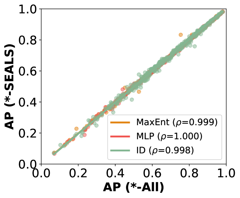
(a) ImageNet

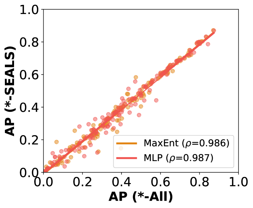
(b) OpenImages

Figure 13: The per-class APs of SEALS ($k=100$) were highly correlated to the baseline approaches (*-All) for active learning on ImageNet (right) and OpenImages (left). On OpenImages with a budget of 2,000 labels, the Pearson’s correlation ($\rho$) between the baseline and SEALS for the average precision of individual classes was 0.986 for MaxEnt and 0.987 for MLP. The least-squares fit had a slope of 0.99 and y-intercept of -0.01. On ImageNet, the correlations were even higher.

Active learning. With a labeling budget of 2,000 examples per concept (~0.31% of $|U|$), all baseline and SEALS approaches ($k=100$) were within 0.011 mAP of the 0.699 mAP achieved with full supervision, as shown in Figure 1(a). In contrast, random sampling (Random-All) only achieved 0.436 mAP. MLP-All, MaxEnt-All, and ID-All achieved mAPs of 0.693, 0.695, and 0.688, respectively, while the SEALS equivalents were all within 0.001 mAP at 0.692, 0.695, and 0.688 respectively and considered less than 7% of the unlabeled data. The resulting selection runtime for MLP-SEALS and MaxEnt-SEALS dropped by over 25$\times$, leading to a 3.6$\times$ speed-up overall (Table 2). The speed-up was even larger for ID-SEALS, ranging from about 45$\times$ at 2,000 labels to 3000$\times$ at 200 labels. Even at a per-class level, the results were highly correlated with Pearson correlation coefficients of 0.9998 or more (Figure 13(a) in the Appendix). The reduced skew from the initial seed set only accounted for a small part of the improvement, as Random-SEALS achieved an mAP of only 0.498.

Active search. As expected, MLP-All and MLP-SEALS significantly outperformed all other selection strategies for active search. At 2,000 labeled examples per concept, both approaches recalled over 74% of the positive examples for each concept at 74.5% and 74.2% recall, respectively. MaxEnt-All and MaxEnt-SEALS had a similar gap of 0.3%, labeling 57.2% and 56.9% of positive examples, while ID-All and ID-SEALS were even closer with a gap of only 0.1% (50.8% vs. 50.9%). Nearly all of the gains in recall are due to the selection strategies rather than the reduced skew in the initial seed, as Random-SEALS increased the recall by less than 1.0% over Random-All.

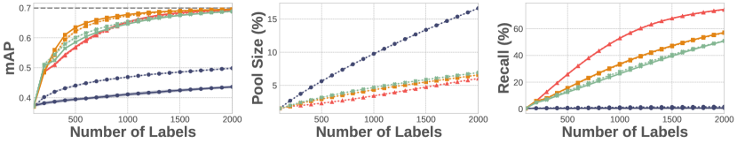
(a) ImageNet ($|U|$=639,906)

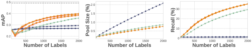
(b) OpenImages ($|U|$=6,816,296)

Figure 1: Active learning and search on ImageNet (top) and OpenImages (bottom). Across datasets and strategies, SEALS with $k=100$ performed similarly to the baseline approach in terms of both the error the model achieved for active learning (left) and the recall of positive examples for active search (right), while only considering a fraction of the data $U$ (middle).

5.3 OpenImages

OpenImages [29] has 7.34 million images from Flickr. However, only 6.82 million images were still available in the training set at the time of writing. The human-verified labels provide partial coverage for over 19,958 classes. Like Kuznetsova et al. [29], we treat examples that are not positively labeled for a given class as negative examples. This label noise makes the task much more challenging, but all of the selection strategies adjust after a few rounds. As a feature extractor, we took ResNet-50 pre-trained on all of ImageNet and used the $l^{2}$ normalized output from the bottleneck layer. As rare concepts, we randomly selected 200 classes with between 100 to 6,817 positive training examples. We reviewed the selected classes and removed 47 classes that overlapped with ImageNet. The remaining 153 classes appeared in 0.002-0.088% of the data. We used the predefined test split for evaluation.

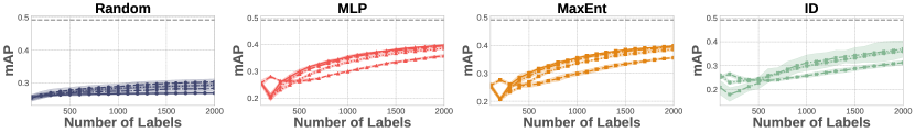
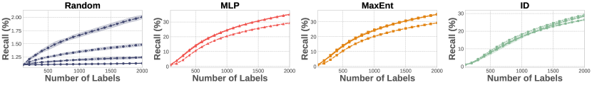
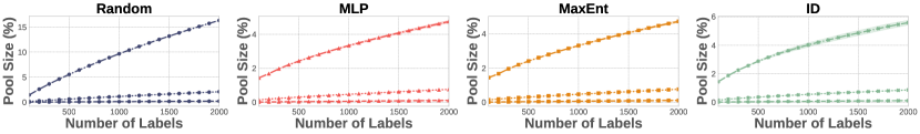
Figure 8: Impact of increasing $k$ on OpenImages ($|U|$=6,816,296). Larger values of $k$ help to close the gap between SEALS and the baseline approach for active learning (top) and active search (middle). However, increasing $k$ also increases the candidate pool size (bottom), presenting a trade-off between labeling efficiency and computational efficiency.

Active learning. At 2,000 labels per concept (~0.029% of $|U|$), MaxEnt-All and MLP-All achieved 0.399 and 0.398 mAP, respectively, while MaxEnt-SEALS and MLP-SEALS both achieved 0.386 mAP and considered less than 1% of the data (Figure 1(b)). This sped-up the selection time by over 180$\times$ and the total time by over 3$\times$, as shown in Table 2. Increasing $k$ to 1,000 significantly narrowed this gap for MaxEnt-SEALS and MLP-SEALS, improving mAP to 0.395, as shown in the Appendix (Figure 8). Moreover, the reduced candidate pool from SEALS made ID tractable on OpenImages, whereas ID-All ran for over 24 hours in wall-clock time without completing a single round (Table 2).

Active search. The gap between the baselines and SEALS was even closer on OpenImages than on ImageNet despite considering a much smaller fraction of the overall unlabeled pool. MLP-All, MLP-SEALS, MaxEnt-SEALS, and MaxEnt-All were all within 0.1% with ~35% recall at 2,000 labels per concept. ID-SEALS had a recall of 29.3% but scaled nearly as well as the linear approaches.

5.4 10 Billion Images

10 billion (10B) publicly shared images from a large internet company were used to test SEALS’ scalability. We used the same pre-trained ResNet-50 model as the OpenImages experiments. We also selected eight additional classes from OpenImages as rare concepts: ‘rat,’ ‘sushi,’ ‘bowling,’ ‘beach,’ ‘hawk,’ ‘cupcake,’ and ‘crowd.’ This allowed us to use the test split from OpenImages for evaluation. Unlike the other datasets, we hired annotators to label images as they were selected and used a proprietary index to achieve low latency retrieval times to capture a real-world setting.

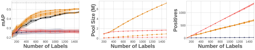
Figure 2: Active learning and search on a de-identified and aggregated dataset of 10 billion publicly shared images. Across strategies, SEALS with $k=10,000$ performed similarly to the baseline approach in terms of both the error the model achieved for active learning (left) and the recall of positive examples for active search (right), while only considering a fraction of the data $U$ (middle).

Active learning. Despite the limited pool size, SEALS performed similarly to the baseline approaches that scanned all 10 billion images. At a budget of 1,500 labels, MaxEnt-SEALS ($k$=10K) achieved a similar mAP to the baseline (0.504 vs. 0.508 mAP), while considering only about 0.1% of the data (Figure 2). This reduction allowed MaxEnt-SEALS to finish selection rounds in just seconds on a single 24-core machine, while MaxEnt-All took several minutes on a cluster with tens of thousands of cores. Unlike the ImageNet and OpenImages experiments, MLP-SEALS performed poorly at this scale because there are likely many redundant or near-duplicate examples of little value.

Active search. SEALS performed well despite considering less than 0.1% of the data and collected two orders of magnitude more positive examples than random sampling.

6 Discussion and Conclusion

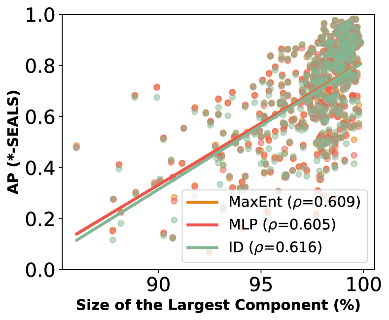
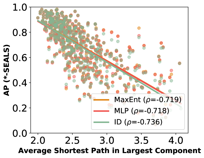
(a) ImageNet

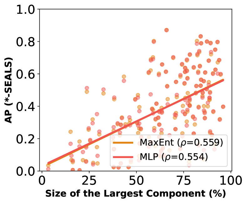
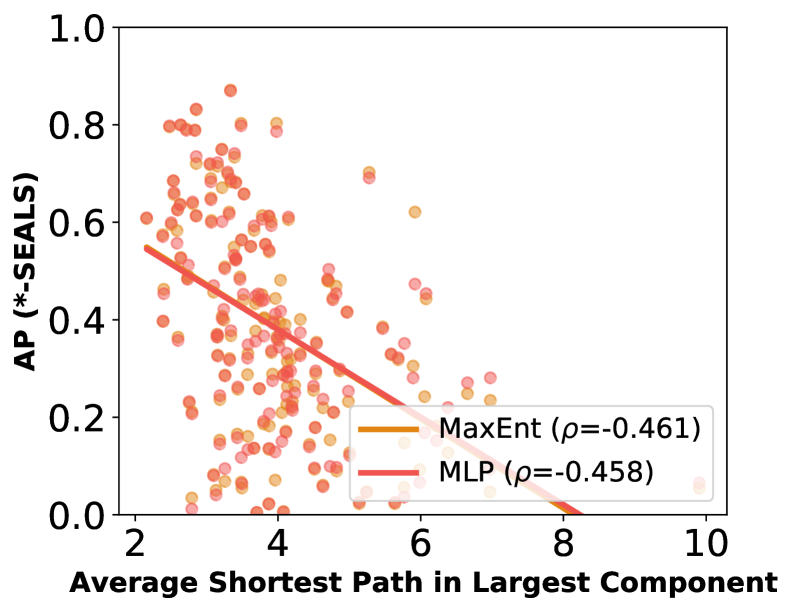
(b) OpenImages

Figure 4: Correlations between AP and measurements of the latent structure of unseen concepts. SEALS ($k=100$) achieved higher APs for classes that formed larger connected components (left) and had shorter paths between examples (right) in ImageNet (top) and OpenImages (bottom).

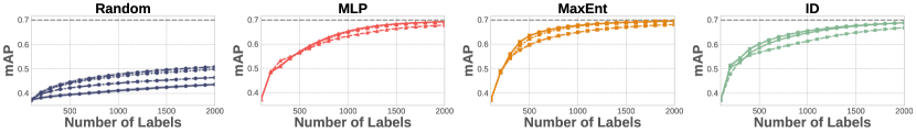
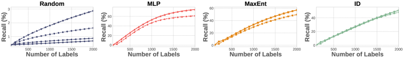
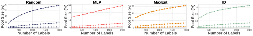
Figure 7: Impact of increasing $k$ on ImageNet ($|U|$=639,906). Larger values of $k$ help to close the gap between SEALS and the baseline approach for active learning (top) and active search (middle). However, increasing $k$ also increases the candidate pool size (bottom), presenting a trade-off between labeling efficiency and computational efficiency.

Latent structure of unseen concepts. To better understand when SEALS works, we analyzed the relationship between average precision and the structure of the nearest neighbor graph across concepts. Overall, SEALS performed better for concepts that formed larger connected components and had shorter paths between examples, as shown in Figure 4. For most concepts in ImageNet, the largest connected component contained the majority of examples, and the paths between examples were very short. These tight clusters explain why so few examples were needed to learn accurate binary concept classifiers, as shown in Section 5, and why SEALS recovered ~74% of positive examples on average while only labeling ~0.31% of the data. If we constructed the candidate pool by randomly selecting examples as in [13], mAP and recall would drop for all strategies (Section 7.8 in the Appendix). The concepts were so rare that the randomly chosen examples were not close to the decision boundary. For OpenImages, rare concepts were more fragmented, but each component was fairly tight, leading to short paths between examples. On a per-class level, concepts like ‘monster truck’ and ‘blackberry’ performed much better than generic concepts like ‘electric blue’ and ‘meal’ that were more scattered (Sections 7.9 and 7.10 in the Appendix). This fragmentation partly explains the gap between SEALS and the baselines in Section 5, and why increasing $k$ closed it. However, even for small values of $k$, SEALS led to significant gains over random sampling, as shown in Figures 7 and 8 in the Appendix.

Conclusion. We introduced SEALS as a simple approach to make the selection rounds of active learning and search methods scale sublinearly with the unlabeled data. Instead of scanning over all of the data, SEALS restricted the candidate pool to the nearest neighbors of the labeled set. Despite this limited pool, we found that SEALS achieved similar average precision and recall while improving computational efficiency by up to three orders of magnitude, enabling web-scale active learning.

7 Appendix

7.1 Broader Impact

Our work attacks both the labeling and computational costs of machine learning and will hopefully make machine learning much more affordable. Instead of being limited to a small number of large teams and organizations with the budget to label data and the computational resources to train on it, SEALS dramatically reduces the barrier to machine learning, enabling small teams or individuals to build accurate classifiers. SEALS does, however, introduce another system component, a similarity search index, which adds some additional engineering complexity to build, tune, and maintain. Fortunately, several highly optimized implementations like Annoy  and Faiss  work reasonably well out of the box. There is a risk that poor embeddings will lead to disjointed components for a given concept. This failure mode may prevent SEALS from reaching all fragments of a concept or take a longer time to do so, as mentioned in Section 6. However, active learning and search methods often involve humans in the loop, which could detect biases and correct them by adding more examples.

7.2 Proof of SEALS under idealized conditions

To begin, we introduce the mathematical setting. Assume the input space is a convex set $\mathcal{X}\subset\mathbb{R}^{d}$ and that the optimal linear classifier $w_{*}\in\mathbb{R}^{d}$ satisfies $\left\lVert w_{*}\right\rVert_{2}=1$. We assume the homogenous setting where $\mathcal{H}_{*}=\{x\in\mathbb{R}^{d}:w_{*}^{\top}x=0\}$ is the hyperplane defining the optimal classification. For each $x\in\mathcal{X}$, let $y_{x}$ denote its associated label and assume that $y_{x}=1$ if $w_{*}^{\top}x\geq 0$ and $y_{x}=-1$ if $w_{*}^{\top}x<0$. Define $\mathcal{X}^{+}=\{x\in\mathcal{X}:w_{*}^{\top}x\geq 0\}$ and $\mathcal{X}^{-}=\{x\in\mathcal{X}:w_{*}^{\top}x<0\}$. Let $\delta>0$ and let $\mathcal{G}=(\mathcal{X},E)$ be a nearest-neighbor graph where we assume that for each $x,x^{\prime}\in\mathcal{X}$, if $\left\lVert x-x^{\prime}\right\rVert_{2}\leq\delta$, then $(x,x^{\prime})\in E$.

Our analysis makes two key assumptions. First, we assume that the classes are linearly separable. Since the SEALS algorithm uses feature embedding, often extracted from a deep neural network, the classes are likely to be almost linearly separable in many applications. Second, we assume a membership query model where the algorithm can query any point belonging to the input space $\mathcal{X}$. Since SEALS is typically applied to datasets with billions of examples, this query model is a reasonable approximation of practice. It should be possible to extend our analysis to the pool-based active learning setting. Suppose there are enough points so that for every possible direction there is at least one point in every $\delta$-nearest neighborhood with a component of size $c\delta$, for some $0<c<1$, in that direction. Then we believe that a bound like that in Theorem 1 should hold by replacing $\delta$ with $c\delta$. Relaxing these two assumptions is left to future theory work.

The main goal of our theory is to quantify the effect of the nearest neighbor restriction. Our analysis considers the modified SEALS procedure described in Algorithm 3. It differs from original SEALS in some minor ways that make it more amenable to analysis, but crucially it too is based on nearest neighbor graph search. First, we introduce some notation. We let $\mathcal{S}_{r}\subset\mathcal{X}\times\{-1,1\}$ consist of the examples and their labels queried until round $r$. We let $\mathcal{S}_{r}^{1}=\{x\in\mathcal{S}_{1}:(x,1)\in\mathcal{S}_{r}\}$ denote the positive examples queried until round $r$ and $\mathcal{S}_{r}^{-1}=\{x\in\mathcal{S}_{1}:(x,-1)\in\mathcal{S}_{r}\}$ the negative examples queried until round $r$. Let $A,B\subset\mathbb{R}^{d}$. The subroutine $\text{MaxMarginSeparator}(A,B)$ finds a maximum margin separator of $A$ and $B$ and returns the hyperplane $H$ and margin $\gamma$: $(H,\gamma)\longleftarrow\text{MaxMarginSeparator}(A,B)$. This is a support vector machine.

Now, we present Algorithm 3. We suppose that the algorithm has an initial set of seed points $\{x_{1,0},\ldots,x_{d-1,0}\}$, with which it initiates $d-1$ nearest neighbor searches. We note that the algorithm could perform $n$ nearest neighbor searches and the analysis would still go through provided that $d-1\leq n=O(d)$, and that the initial set of labeled points $\mathcal{S}_{r}$ may be larger than $d-1$. At each round $r$, Algorithm 3 queries one unlabeled neighbor from each set $C_{i,r}$, $i=1,\dots,d-1$ (at $r=0$ these sets are the seed points themselves). The decision rule is as follows: first, for each $x\in C_{i,r}$, the algorithm computes a max-margin separating hyperplane $H_{x}$ separating $x$ from the examples with opposing labels. Second, the algorithm selects the example with the smallest margin $\bar{x}_{i,r}$ and queries a neighbor of $\bar{x}_{i,r}$ that is closest to $H_{\bar{x}_{i,r}}$. This is similar to using MaxEnt uncertainty sampling in SEALS. In Algorithm 3, $\operatorname*{arg\,min}_{x^{\prime}:(\bar{x}_{i,r},x^{\prime})\in E}\,\mathrm{dist}(x^{\prime},H_{\bar{x}_{i,r},r})$ may contain several examples if $\mathrm{dist}(\bar{x}_{i,r},H_{\bar{x}_{i,r},r})\leq\delta$. In this case, we tiebreak by letting $\tilde{x}_{i,r}$ be the projection of $\bar{x}_{i,r}$ onto $H_{\bar{x}_{i,r},r}$.

Algorithm 3 Modified SEALS

1:Input: seed labeled examples $\mathcal{S}_{1}\subset\mathcal{X}\times\{-1,1\}$

2:$r=1$

3:Initialize the clusters $C_{i,r}=\{x_{i,0}\}$ for $i=1,\ldots,d-1$

4:for $r=1,2,\ldots$ do

5:     for $i=1,\ldots,d-1$ do

6:         $(H_{x,r},\gamma_{x,r})=\text{MaxMarginSeparator}(\mathcal{S}_{r}^{-y_{x}},x)$ for all $x\in C_{i,r}$

7:         Let $\bar{x}_{i,r}\in\operatorname*{arg\,min}_{x\in C_{i,r}}\gamma_{x,r}$ and $\widetilde{x}_{i,r}\in\operatorname*{arg\,min}_{x^{\prime}:(\bar{x}_{i,r},x^{\prime})\in E}\mathrm{dist}(x^{\prime},H_{\bar{x}_{i,r},r})$

8:         Query $\widetilde{x}_{i,r}$

9:         Update $\mathcal{S}_{r+1}=\mathcal{S}_{r}\cup\{(\widetilde{x}_{i,r},y_{\widetilde{x}_{i,r}})\}$ and $C_{i,r+1}=C_{i,r}\cup\{\widetilde{x}_{i,r}\}$

10:     end for

11:     Fit a homogenous max-margin separator with normal vector $\widehat{w}_{r+1}$ to $\mathcal{S}_{r+1}$ 

12:end for

We actually restate the Theorem 1 a bit more formally in Theorem 2, below.

Theorem 2.

Let $\epsilon>0$. Let $x_{1,0},\ldots,x_{d-1,0}$ denote the seed points. Define $\gamma_{i}=\mathrm{dist}(x_{i,0},{{\tt{conv}}}(\mathcal{S}^{-y_{x_{i,0}}}_{1}))$ for $i\in[d-1]$, where ${\tt{conv}}(\mathcal{S}^{-y_{x_{i,0}}}_{1})$ is the convex hull of the points $\mathcal{S}^{-y_{x_{i,0}}}_{1}.$ Then, after Algorithm 3 makes $\max_{i\in[d-1]}d(\frac{\gamma_{i}}{\delta}+2\log(\frac{2d\delta}{\epsilon\min(\sigma,1)})))$ queries, $\left\lVert\widehat{w}_{r}-w_{*}\right\rVert\leq\epsilon.$

The constant $\sigma$ is a measure of the diversity of the initial seed examples, which we now define. For $i\in[d-1]$, define the set

$$\mathcal{Z}_{i} =\{z\in\mathbb{R}^{d}:\left\lVert z-x_{i,0}\right\rVert\leq\gamma_{i}+2\delta+\epsilon\text{ and }\mathrm{dist}(z,\{x\in\mathbb{R}^{d}:x^{\top}w_{*}=0\})\leq\epsilon\}.$$

Define

$$\sigma :=\min_{z_{i}\in\mathcal{Z}_{i}:\forall i\in[d-1]}\sigma_{d-1}([z_{1}\ldots z_{d-1}]).$$

where $\sigma_{d-1}$ denotes the $(d-1)$th singular value of the matrix $[z_{1}\ldots z_{d-1}]$.

Here we give a simple example where $\sigma=\Omega(1)$ so as to provide intuition, although there are a wide variety of such cases.

Example 1.

Let $\epsilon\in(0,1)$. Let $\mathcal{X}=\mathbb{R}^{d}$, $w^{*}=e_{1}$, $\delta=1/2$. Let $M\geq 6\sqrt{d-1}$. Suppose the seed examples are $x_{i,0}=e_{1}+Me_{i+1}$ for $i\in[d-1]$ and suppose the algorithm is given additional examples $v_{i}=-e_{1}+Me_{i+1}\in\mathcal{S}_{0}^{-1}$ for $i\in[d-1]$. Then, $\sigma\geq 1$.

Proof of Example 1.

Note that $\gamma_{i}=2$ for all $i\in[d-1]$. Define the matrix

$$Z =\begin{pmatrix}z_{1}^{\top}\\ \vdots\\ z_{d-1}^{\top}\end{pmatrix}$$

such that $\left\lVert z_{i}-x_{i,0}\right\rVert\leq\gamma_{i}+2\delta+\epsilon,\,\forall i\in[d-1]$. We may write $z_{i}=x_{i,0}+v_{i}$ where $\left\lVert v_{i}\right\rVert\leq\gamma_{i}+2\delta+\epsilon$. Courant-Fisher’s min-max theorem implies that $s_{d-1}(Z)=\max_{\dim E=d-1}\min_{u\in\text{span}(E):\left\lVert u\right\rVert=1}\left\lVert Zu\right\rVert$ where $E\subset\mathbb{R}^{d}$. Therefore, taking $E=\{e_{2},\ldots,e_{d}\}$, it suffices to lower bound $\left\lVert Zu\right\rVert$ for any $u\in\text{span}(e_{2},\ldots,e_{d})$ with $\left\lVert u\right\rVert=1$. Since $\left\lVert u\right\rVert=1$, there exists $j\in\{2,\ldots,d\}$ such that $|u_{j}|\geq\frac{1}{\sqrt{d-1}}$. Suppose wlog that $u_{j}\geq\frac{1}{\sqrt{d-1}}$ (the other case is similar). Then, by Cauchy-Schwarz,

$$\left\lVert Zu\right\rVert \geq\max_{i\in[d-1]}|z_{i}^{\top}u|$$

$$\geq(e_{1}+Me_{j}+v_{j-1})^{\top}u$$

$$\geq M\frac{1}{\sqrt{d}}-1-\gamma_{i}-2\delta-\epsilon$$

$$\geq\frac{M}{\sqrt{d}}-5$$

$$\geq 1.$$

∎

Now, we turn to the proof of Theorem 2. In the interest of using more compact notation, we define for all $i\in[d-1]$ and $r\in\mathbb{N}$

$$\rho_{i,r}:=\mathrm{dist}(\bar{x}_{i,r},{\tt{conv}}(\mathcal{S}_{r}^{-y_{\bar{x}_{i,r}}})).$$

In words, $\rho_{i,r}$ is the distance of the example queried in nearest neighbor search $i$ and at round $r$, $\bar{x}_{i,r}$, to the convex hull of $\mathcal{S}_{r}^{-y_{\bar{x}_{i,r}}}$, the examples with opposite labels from $\bar{x}_{i,r}$.

Proof of Theorem 2.

Step 1: Bounding the number of queries to find points near the decision boundary. Define $\bar{\epsilon}=\frac{\min(\sigma,1)\epsilon^{2}}{2\sqrt{d}}$, where $\sigma$ is defined as in the Theorem statement. We assume $\sigma>0$ for the remainder of the proof. Let $C_{i,r}=\{x_{i,0},x_{i,1},\ldots,x_{i,r}\}$ where $x_{i,l}$ is the queried example in the $l$th round. We show that for all $r\geq\max_{i\in[d-1]}\frac{\gamma_{i}}{\delta}+\log(\frac{2\delta}{\bar{\epsilon}})$ , for all $i\in[d-1]$, $\rho_{i,r}\leq\bar{\epsilon}$.

Fix $i\in[d-1]$. Define

$$E_{r}=\{\text{at round }r,\rho_{i,r}\leq\bar{\epsilon}\}.$$

We have that

$$\sum_{r\in\mathbb{N}}\mathbf{1}\{E_{r}^{c}\} =\sum_{r\in\mathbb{N}}\mathbf{1}\{E_{r}^{c}\cap\{\rho_{i,r}\geq 2\delta\}\}$$

$$\hskip 56.9055pt+\mathbf{1}\{E_{r}^{c}\cap\{\rho_{i,r}<2\delta\}\}$$

If $\rho_{i,r}\geq 2\delta$, we have by Lemma 1 that

$$\rho_{i,r+1}\leq\rho_{i,r}-\delta.$$

This implies that

$$\sum_{r\in\mathbb{N}}\mathbf{1}\{E_{r}^{c}\ \cap\{\rho_{i,r}\geq 2\delta\}\}\leq\frac{\gamma_{i}}{\delta}.$$

Now, suppose that $\rho_{i,r}<2\delta$. Then, by Lemma 1, we have that

$$\rho_{i,r+1}\leq\frac{\rho_{i,r}}{2}.$$

Unrolling this recurrence implies that

$$\sum_{r\in\mathbb{N}}\mathbf{1}\{E_{r}^{c}\ \cap\{\rho_{i,r}<2\delta\}\}\leq\log(\frac{2\delta}{\bar{\epsilon}}).$$

Putting it altogether, we have that

$$\sum_{r\in\mathbb{N}}\mathbf{1}\{E_{r}^{c}\}\leq\frac{\gamma_{i}}{\delta}+\log(\frac{2\delta}{\bar{\epsilon}}).$$

This implies that after $\max_{i\in[d-1]}\frac{\gamma_{i}}{\delta}+\log(\frac{2\delta}{\bar{\epsilon}})$ queries, we have that for all $i\in[d-1]$, $\rho_{i,r}:=\mathrm{dist}(\bar{x}_{i,r},{\tt{conv}}(\mathcal{S}_{r}^{-y_{x_{i,r}}}))\leq\bar{\epsilon}$.

Step 2: Showing $\left\lVert x_{i,0}-x_{i,r}\right\rVert\leq\gamma_{i}+2\delta$ for all $i\in[d-1]$. Fix $i\in[d-1]$. Let $C_{i,r}=\{x_{i,0},x_{i,1},\ldots,x_{i,r}\}$ where $x_{i,l}$ is the queried example in the $l$th round. Note there exists a path of length at most $r$ in the nearest neighbor graph on the nodes in $C_{i,r}$ between $x_{i,0}$ and $x_{i,r}$. In the worst case, this path consists of $x_{i,0},x_{i,2},\ldots,x_{i,r}$ with $x_{i,s}$ being the child of $x_{i,s-1}$ and thus we suppose that this is the case wlog.

By the argument in step 1 of the proof, we have that after at most $\bar{k}=\frac{\gamma_{i}}{\delta}$ rounds,

$$\mathrm{dist}(x_{i,\bar{k}},{\tt{conv}}(\mathcal{S}_{r}^{-y_{x_{i,\bar{k}}}}))\leq 2\delta.$$

For $s\leq\bar{k}$, we have that $\left\lVert x_{i,s}-x_{i,{s-1}}\right\rVert\leq\delta$ by definition of the nearest neighbor graph. Now, consider $s\geq\bar{k}$. By Lemma 2, we have that $\left\lVert x_{i,s+1}-x_{i,{s}}\right\rVert\leq\frac{\left\lVert x_{i,s}-x_{i,{s-1}}\right\rVert}{2}$ and $\left\lVert x_{i,\bar{k}+1}-x_{i,{\bar{k}}}\right\rVert\leq\delta$. Therefore,

$$\left\lVert x_{i,r}-x_{i,0}\right\rVert =\left\lVert\sum_{s=1}^{r-1}x_{i,s+1}-x_{i,{s}}\right\rVert$$

$$\leq\sum_{s=1}^{r-1}\left\lVert x_{i,s+1}-x_{i,{s}}\right\rVert$$

$$\leq\bar{k}\max_{s\leq\bar{k}}\left\lVert x_{i,s+1}-x_{i,{s}}\right\rVert+\sum_{s=\bar{k}+1}^{r-1}\left\lVert x_{i,s+1}-x_{i,{s}}\right\rVert$$

$$\leq\frac{\gamma_{i}}{\delta}\delta+\delta\sum_{s=\bar{k}+1}^{r-1}\frac{1}{2^{-s}}$$

$$\leq\gamma_{i}+2\delta.$$

Step 3: for all $i\in[d-1]$, there exists $z_{i}\in\mathcal{Z}_{i}$ such that $\widehat{w}_{r}^{\top}z_{i}=0$. We have that $\rho_{i,r}\leq\bar{\epsilon}$ for all $i\in[d-1]$ and $\left\lVert x_{i,0}-x_{i,r}\right\rVert\leq\gamma_{i}+2\delta$ for all $i\in[d-1]$. Now, we show that there exists $z_{i}\in\mathcal{Z}_{i}$ such that $\widehat{w}_{r}^{\top}z_{i}=0$. Fix $i\in[d-1]$. Suppose $\widehat{w}^{\top}_{r}\bar{x}_{i,r}>0$ (the other case is similar). Then, $\rho_{i,r}\leq\bar{\epsilon}$ implies that there exists $\bar{x}\in{\tt{conv}}(\mathcal{S}_{r}^{-1})$ such that $\left\lVert\bar{x}_{i,r}-\bar{x}\right\rVert\leq\bar{\epsilon}$. Then, since $\widehat{w}_{r}$ separates $\mathcal{S}_{r}^{-1}$ and $\mathcal{S}_{r}^{1}$, $\widehat{w}^{\top}_{r}\bar{x}\leq 0$. Now, there exists $z_{i}\in{\tt{conv}}(\bar{x}_{i,r},\bar{x})$ such that $z_{i}^{\top}\widehat{w}_{r}=0$. By the triangle inequality, we have that $\left\lVert x_{i,0}-z_{i}\right\rVert\leq\gamma_{i}+2\delta+\epsilon$, and $\mathrm{dist}(z_{i},\{x:w_{*}^{\top}x=0\})\leq\bar{\epsilon}\leq\epsilon$, thus, $z_{i}\in\mathcal{Z}_{i}$ for all $i\in[d-1]$, completing this step.

Step 4: Pinning down $w_{*}$. Since $\sigma>0$, and each $z_{i}\in\mathcal{Z}_{i}$, we have that $z_{1},\ldots,z_{d-1}$ are linearly independent. Then, we can write $w_{*}=\sum_{i=1}^{d-1}\beta_{i}z_{i}+\beta_{d}\widehat{w}_{r}$ for $\beta_{1},\ldots,\beta_{d}\in\mathbb{R}$ where we used that $\widehat{w}_{r}$ is orthogonal to $z_{1},\ldots,z_{d-1}$ by construction of $z_{1},\ldots,z_{d-1}$. Note that $\widehat{w}_{r}^{\top}w_{*}=\widehat{w}_{r}^{\top}(\sum_{i=1}^{d-1}\beta_{i}z_{i}+\beta_{d}\widehat{w}_{r})=\beta_{d}$. Let $Pw_{*}$ denote the projection of $w_{*}$ onto $\text{span}(z_{1},\ldots,z_{d-1})$. Defining the matrix $Z=[z_{1}\,z_{2}\,\ldots\,z_{d-1}]$ and $\beta=(\beta_{1}\,\ldots,\beta_{d-1})^{\top}$, we can write $Pw_{*}=Z\beta$. Let $Z=U\Sigma V^{\top}$ denote the SVD of $Z$ and $Z^{\dagger}=V\Sigma^{\dagger}U^{\top}$ the pseudoinverse. Note that $Z^{\dagger}Pw_{*}=\beta$. Then,

$$\left\lVert\beta\right\rVert=\left\lVert Z^{\dagger}Pw_{*}\right\rVert \leq\max_{i=1,2,\ldots,d-1}\sigma_{i}(Z^{\dagger})=\frac{1}{\sigma_{d-1}(Z)}.$$ (1)

We note that $\mathrm{dist}(z_{i},\{x:w_{*}^{\top}x=0\})\leq\bar{\epsilon}$ implies that $|w_{*}^{\top}z_{i}|\leq\bar{\epsilon}$ for $i=1,2,\ldots,d-1$. Then, we have that

$$1 =w_{*}^{\top}w_{*}$$

$$=\sum_{i=1}^{d-1}\beta_{i}w_{*}^{\top}x_{i}+\beta_{d}w_{*}^{\top}\widehat{w}_{r}$$

$$=\sum_{i=1}^{d-1}\beta_{i}w_{*}^{\top}x_{i}+(w_{*}^{\top}\widehat{w}_{r})^{2}$$ (2)

$$\leq\left\lVert\beta\right\rVert_{1}\bar{\epsilon}+(w_{*}^{\top}\widehat{w}_{r})^{2}$$ (3)

$$\leq\sqrt{d}\left\lVert\beta\right\rVert_{2}\bar{\epsilon}+(w_{*}^{\top}\widehat{w}_{r})^{2}$$ (4)

$$\leq\frac{\sqrt{d}\bar{\epsilon}}{\sigma_{d-1}([z_{1}\ldots z_{d-1}])}+(w_{*}^{\top}\widehat{w}_{r})^{2}$$ (5)

$$\leq\frac{\sqrt{d}\bar{\epsilon}}{\sigma}+(w_{*}^{\top}\widehat{w}_{r})^{2}$$ (6)

where equation 2 follows by plugging in the previously derived $\beta_{d}=w_{*}^{\top}\widehat{w}_{r}$, equation 3 follows by Holder’s inequality, equation 4 follows by $\left\lVert\cdot\right\rVert_{1}\leq\sqrt{d}\left\lVert\cdot\right\rVert_{2}$, equation 5 follows by equation 1, and equation 6 follows by the definition of $\sigma$. Rearranging, we have that

$$w_{*}^{\top}\widehat{w}_{r} =|w_{*}^{\top}\widehat{w}_{r}|$$ (7)

$$\geq\sqrt{1-\frac{\sqrt{d}\bar{\epsilon}}{\sigma}}$$

$$\geq 1-\frac{\sqrt{d}\bar{\epsilon}}{\sigma}$$ (8)

$$\geq 1-\frac{\epsilon^{2}}{2}$$ (9)

where equation 7 follows by the definition of $\widehat{w}_{r}$, in equation 8 we use that fact that $1-\frac{\sqrt{d}\bar{\epsilon}}{\sigma}\leq 1$ and in equation 9 we use the definition of $\bar{\epsilon}$. Now, we have that

$$\left\lVert\widehat{w}_{r}-w_{*}\right\rVert^{2}=2(1-\widehat{w}_{r}^{\top}w_{*})\leq\epsilon^{2},$$

proving the result.

∎

In Lemma 1, we show that at each round $\bar{x}_{i,r}$ moves closer to the labeled examples of the opposite class. The main idea behind the proof is that the algorithm can always choose a point $\tilde{x}_{i,r}$ in the direction orthogonal to the hyperplane $H_{\bar{x}_{i,r},r}$, thus guaranteeing a reduction in $\rho_{i,r}$. Early in the execution of Algorithm 3, the nearest neighbor graph constrains which points are chosen, leading to a reduction in $\rho_{i,r}$ of $\delta$. However, once $\bar{x}_{i,r}$ is close enough to the labeled examples of the opposite class, precisely once $\rho_{i,r}<2\delta$, the algorithm begins selecting points that lie on $H_{\bar{x}_{i,r},r}$ at each round, halving $\rho_{i,r}$ at each round.

Lemma 1.

Fix $i\in[d-1]$. Fix $r\in\mathbb{N}$.

1. If $\rho_{i,r}\geq 2\delta$, then

   $$\rho_{i,r+1}\leq\rho_{i,r}-\delta.$$

2. If $\rho_{i,r}<2\delta$, then

   $$\rho_{i,r+1}\leq\frac{\rho_{i,r}}{2}.$$

Proof.

1. Let $\bar{x}_{i,r}=\min_{x\in C_{i,r}}\gamma_{x,r}$ as defined in the algorithm. Wlog, suppose that $\bar{x}_{i,r}\in\mathcal{X}^{+}$. By Lemma 2, there exists $z\in{\tt{conv}}(\mathcal{S}_{r}^{-1})$ such that $\tilde{x}_{i,r}=\bar{x}_{i,r}+\alpha\frac{(z-\bar{x}_{i,r})}{\left\lVert z-\bar{x}_{i,r}\right\rVert}$ for some $\alpha\leq\delta$.

Let $\beta=\frac{\alpha}{\left\lVert z-\bar{x}_{i,r}\right\rVert}$. Then,

$$\left\lVert\tilde{x}_{i,r}-z\right\rVert =\left\lVert\bar{x}_{i,r}+\beta(z-\bar{x}_{i,r})-z\right\rVert$$

$$=\left\lVert(1-\beta)\bar{x}_{i,r}-z\right\rVert$$

$$=(1-\beta)\left\lVert\bar{x}_{i,r}-z\right\rVert$$

$$=\left\lVert\bar{x}_{i,r}-z\right\rVert-\alpha.$$

If $\mathrm{dist}(\bar{x}_{i,r},\mathcal{S}_{r}^{-1})\geq 2\delta$, Lemma 2 implies that $\alpha=\delta$ and we have that

$$\left\lVert\tilde{x}_{i,r}-z\right\rVert=\left\lVert\bar{x}_{i,r}-z\right\rVert-\delta=\mathrm{dist}(\bar{x}_{i,r},{\tt{conv}}(\mathcal{S}_{r}^{-1}))-\delta$$

Thus, if $\tilde{x}_{i,r}\in\mathcal{X}^{+}$, using the definition of $\bar{x}_{i,r+1}$, we have that

$$\rho_{i,r+1} =\mathrm{dist}(\bar{x}_{i,r+1},{\tt{conv}}(\mathcal{S}_{r+1}^{-y_{\bar{x}_{i,r+1}}}))$$

$$\leq\mathrm{dist}(\tilde{x}_{i,r},{\tt{conv}}(\mathcal{S}_{r}^{-1}))$$

$$\leq\mathrm{dist}(\bar{x}_{i,r},{\tt{conv}}(\mathcal{S}_{r}^{-1}))-\delta$$

$$=\rho_{i,r}-\delta.$$

On the other hand, if $\tilde{x}_{i,r}\in\mathcal{X}^{-}$, we have that

$$\rho_{i,r+1} =\mathrm{dist}(\bar{x}_{i,r+1},{\tt{conv}}(\mathcal{S}_{r+1}^{-y_{\bar{x}_{i,r+1}}}))$$

$$\leq\mathrm{dist}(\tilde{x}_{i,r},{\tt{conv}}(\mathcal{S}_{r}^{1}))$$

$$\leq\delta$$

$$\leq\mathrm{dist}(\bar{x}_{i,r},{\tt{conv}}(\mathcal{S}_{r}^{-1}))-\delta$$

which also shows the claim.

2. Now, suppose that $\mathrm{dist}(\bar{x}_{i,r},{\tt{conv}}(\mathcal{S}_{r+1}^{-1}))<2\delta$. Then, by Lemma 2, we have that $\alpha=\frac{\left\lVert z-\bar{x}_{i,r+1}\right\rVert}{2}<\delta$, implying that

$$\rho_{i,r+1} =\mathrm{dist}(\bar{x}_{i,r+1},{\tt{conv}}(\mathcal{S}_{r}^{-y_{\bar{x}_{i,r+1}}})$$

$$\leq\left\lVert\tilde{x}_{i,r}-z\right\rVert$$

$$=\left\lVert\tilde{x}_{i,r}-\bar{x}_{i,r}\right\rVert$$

$$=\left\lVert\bar{x}_{i,r}-z\right\rVert/2$$

$$=\frac{\mathrm{dist}(\bar{x}_{i,r},{\tt{conv}}(\mathcal{S}_{r}^{-1}))}{2}$$

$$=\frac{\rho_{i,r}}{2}$$

and therefore the result.

∎

Lemma 2 characterizes the example, $\tilde{x}_{i,r}$, queried by Algorithm 3. It shows that $\tilde{x}_{i,r}$ always belongs to a line segment connecting $\bar{x}_{i,r}$ to some point, $z$, in the convex hull of labeled points of the opposite class, ${\tt{conv}}(\mathcal{S}_{r+1}^{-y_{\bar{x}_{i,r}}})$. If $\rho_{i,r}\geq 2\delta$, then $\tilde{x}_{i,r}$ moves $\delta$ along this line segment towards $z$ and if $\rho_{i,r}<2\delta$, $\tilde{x}_{i,r}$ is the midpoint of this line segment.

Lemma 2.

Fix round $r\in\mathbb{N}$. There exists $z\in{\tt{conv}}(\mathcal{S}_{r+1}^{-y_{\bar{x}_{i,r}}})$ such that the following holds. If $\rho_{i,r}\geq 2\delta$, then $\tilde{x}_{i,r}=\bar{x}_{i,r}+\delta\frac{(z-\bar{x}_{i,r})}{\left\lVert z-\bar{x}_{i,r}\right\rVert}$. If $\rho_{i,r}<2\delta$, then $\tilde{x}_{i,r}=\frac{\bar{x}_{i,r}+z}{2}$.

Proof.

Step 1: A formula for the max-margin separator.

Without loss of generality, suppose that $\bar{x}_{i,r}\in\mathcal{X}^{+}$ (the other case is similar). Let $\bar{w}\in\mathbb{R}^{d}$, $\bar{b}\in\mathbb{R}$, and $\bar{t}\in\mathbb{R}$ denote the optimal solutions of the optimization problem

$$\max_{w\in\mathbb{R}^{d},b\in\mathbb{R},t\in\mathbb{R}}\, t$$ (10)

s.t. $$\bar{x}_{i,r}^{\top}w-b\leq-t$$

$$x^{\top}w-b\geq t\,\forall x\in\mathcal{S}_{r+1}^{-1}$$

$$\left\lVert w\right\rVert_{2}\leq 1.$$

Then, $\bar{w}\in\mathbb{R}^{d}$ and $\bar{b}\in\mathbb{R}$ define the max-margin separator separating $\bar{x}_{i,r}$ from $\mathcal{S}_{r+1}^{-1}$. We note that by Lemma 3, $\bar{w}$ and $\bar{b}$ are the unique solutions up to scaling. By Section 8.6.1. in [8], equation 10 has the same value as

$$\min_{\alpha_{j}} \frac{1}{2}\left\lVert\sum_{j:x_{j}\in\mathcal{S}_{r+1}^{-1}}\alpha_{j}x_{j}-\bar{x}_{i,r}\right\rVert$$ (11)

s.t. $$\alpha_{j}\geq 0\,\forall j$$

$$\sum_{j}\alpha_{j}=1$$

Let $\{\tilde{\alpha}_{j}\}$ attain the maximum in the above optimization problem, which exists since the domain is compact and the objective function is continuous. Define $\tilde{x}=\sum_{j:x_{j}\in\mathcal{S}_{r+1}^{-1}}\tilde{\alpha}_{j}x_{j}$ and

$$\tilde{w} =\frac{\tilde{x}-\bar{x}_{i,r}}{\left\lVert\tilde{x}-\bar{x}_{i,r}\right\rVert}$$

$$\tilde{b} =\frac{\left\lVert\tilde{x}\right\rVert^{2}-\left\lVert\bar{x}_{i,r}\right\rVert^{2}}{2\left\lVert\tilde{x}-\bar{x}_{i,r}\right\rVert}$$

We claim that $\tilde{w}=\bar{w}$ and $\tilde{b}=\bar{b}$. First, we show that that there exists $\tilde{t}\in\mathbb{R}$ such that $(\tilde{w},\tilde{b},\tilde{t})$ satisfy the constraints in equation 10. Arithmetic shows that $\tilde{w}^{\top}\tilde{x}-\tilde{b}>0$ and $\tilde{w}^{\top}\bar{x}_{i,r}-\tilde{b}<0$. Since $\tilde{x}$ is the projection of $\bar{x}_{i,r}$ onto ${\tt{conv}}(\mathcal{S}^{+}_{r})$, by the Projection Lemma, we have that

$$(\tilde{x}-\bar{x}_{i,r})^{\top}x\geq(\tilde{x}-\bar{x}_{i,r})^{\top}\tilde{x}$$

for all $x\in{\tt{conv}}(\mathcal{S}^{+}_{r})$. Thus, for all $x\in{\tt{conv}}(\mathcal{S}^{+}_{r})$, we have that

$$\tilde{w}^{\top}x-\tilde{b}\geq\tilde{w}^{\top}\tilde{x}-\tilde{b}>0.$$

We conclude that there exists $\tilde{t}\in\mathbb{R}$ such that $(\tilde{w},\tilde{b},\tilde{t})$ satisfy the constraints in equation 10.

We have that

$$\tilde{w}^{\top}\bar{x}_{i,r}-\tilde{b}=\frac{1}{\left\lVert\tilde{x}-\bar{x}_{i,r}\right\rVert}(\bar{x}_{i,r}^{\top}(\tilde{x}-\bar{x}_{i,r})-\frac{\left\lVert\tilde{x}\right\rVert^{2}-\left\lVert\bar{x}_{i,r}^{2}\right\rVert}{2})=-\frac{1}{2}\left\lVert\bar{x}_{i,r}-\tilde{x}\right\rVert.$$

A similar calculation shows that $\tilde{w}^{\top}x-\tilde{b}\geq\frac{1}{2}\left\lVert\bar{x}_{i,r}-\tilde{x}\right\rVert$ for all $x\in{\tt{conv}}(\mathcal{S}^{+}_{r})$. Thus, putting $\tilde{t}=\frac{1}{2}\left\lVert\tilde{x}-\bar{x}_{i,r}\right\rVert$, $(\tilde{w},\tilde{b},\tilde{t})$ is feasible to equation 10. By the equivalence in value of equation 10 and equation 11 and the definition of $\tilde{x}$, we have that $\frac{1}{2}\left\lVert\tilde{x}-\bar{x}_{i,r}\right\rVert=\bar{t}$. Thus, by uniqueness of $\bar{w}$ and $\bar{b}$, we have that $\tilde{w}=\bar{w}$ and $\tilde{b}=\bar{b}$.

Step 2: Putting it together. We have shown that $\tilde{w}$ and $\tilde{b}$ define the max-margin separator. Let $P\bar{x}_{i,r}$ denote the projection of $\bar{x}_{i,r}$ onto $H:=\{z\in\mathbb{R}^{d}:\tilde{w}^{\top}z=\tilde{b}\}$. We have that

$$P\bar{x}_{i,r} =\bar{x}_{i,r}+(\frac{\left\lVert\tilde{x}\right\rVert^{2}-\left\lVert\bar{x}_{i,r}\right\rVert^{2}}{2\left\lVert\tilde{x}-\bar{x}_{i,r}\right\rVert}-(\frac{\tilde{x}-\bar{x}_{i,r}}{\left\lVert\tilde{x}-\bar{x}_{i,r}\right\rVert})^{\top}\bar{x}_{i,r}\frac{\tilde{x}-\bar{x}_{i,r}}{\left\lVert\tilde{x}-\bar{x}_{i,r}\right\rVert}$$

$$=\frac{\tilde{x}+\bar{x}_{i,r}}{2}.$$

Suppose that $\mathrm{dist}(\bar{x}_{i,r},{\tt{conv}}(\mathcal{S}_{r+1}^{-y_{\bar{x}_{i,r}}}))\geq 2\delta$. Then, we have that $\mathrm{dist}(\bar{x}_{i,r},H)>2\delta$. It can be easily seen that $\tilde{x}_{i,r}=\operatorname*{arg\,min}_{x:\left\lVert x-\bar{x}_{i,r}\right\rVert\leq\delta}\mathrm{dist}(x,H)=\bar{x}_{i,r}+\delta\frac{\tilde{x}-\bar{x}_{i,r}}{\left\lVert\tilde{x}-\bar{x}_{i,r}\right\rVert}$. Note that $\bar{x}_{i,r}+\delta\frac{\tilde{x}-\bar{x}_{i,r}}{\left\lVert\tilde{x}-\bar{x}_{i,r}\right\rVert}\in\mathcal{X}$, since $\bar{x}_{i,r},\tilde{x}\in\mathcal{X}$ and $\mathcal{X}$ is convex.

Similarly, if $\mathrm{dist}(\bar{x}_{i,r},{\tt{conv}}(\mathcal{S}_{r+1}^{-y_{\bar{x}_{i,r}}}))<2\delta$, Then, we have that $\mathrm{dist}(\bar{x}_{i,r},H)<\delta$. Then, by definition of $\tilde{x}_{i,r}$ we have that $\tilde{x}_{i,r}=\frac{\tilde{x}+\bar{x}_{i,r}}{2}\in\mathcal{X}$, where we have that $\frac{\tilde{x}+\bar{x}_{i,r}}{2}\in\mathcal{X}$ by convexity of $\mathcal{X}$.

∎

The following result shows that the max-margin separator is unique, and is a standard result on SVMs.

Lemma 3.

Let $A,B\subset\mathbb{R}^{d}$ be disjoint, closed, and convex. The max-margin separator separating $A$ and $B$ is unique.

Proof.

There exists a separating hyperplane between $A$ and $B$ by the separating hyperplane Theorem. By a standard argument, the optimization problem for the max-margin separator can be stated as

$$\min_{w\in\mathbb{R}^{d},b\in\mathbb{R}} \left\lVert w\right\rVert^{2}$$

s.t. $$w^{\top}x+b\geq 1\,\forall x\in A$$

$$w^{\top}x+b\leq-1\,\forall x\in B.$$

This is a convex optimization problem with a strongly convex objective and, therefore, has a unique solution. ∎

7.3 SEALS with Querying Anywhere Capability

Algorithm 4 Modified SEALS: Project onto Hyperplane

1:Input: seed labeled points $\mathcal{S}_{1}\subset\mathcal{X}\times\{-1,1\}$   $r=1$

2:Initialize the clusters $C_{i,r}=\{x_{i,0}\}$ for $i=1,\ldots,d-1$

3:for $r=1,2,\ldots$ do

4:     for $i=1,\ldots,d-1$ do

5:         $(H_{x,r},\gamma_{x,r})=\text{MaxMarginSeparator}(\mathcal{S}_{r}^{-y_{x}},x)$ for all $x\in C_{i,r}$

6:         Let $\bar{x}_{i,r}\in\operatorname*{arg\,min}_{x\in C_{i,r}}\gamma_{x,r}$ and $\widetilde{x}_{i,r}\in\operatorname*{arg\,min}_{x^{\prime}}\mathrm{dist}(x^{\prime},H_{\bar{x}_{i,r},r})$

7:         Query $\widetilde{x}_{i,r}$

8:         Update $\mathcal{S}_{r+1}=\mathcal{S}_{r}\cup\{(\widetilde{x}_{i,r},y_{\widetilde{x}_{i,r}})\}$ and $C_{i,r+1}=C_{i,r}\cup\{\widetilde{x}_{i,r}\}$

9:     end for

10:     Fit a homogenous max-margin separator with normal vector $\widehat{w}_{r+1}$ to $\mathcal{S}_{r+1}$

11:end for

The data structure used in SEALS enables queries of the $k$-nearest neighbors of any point in the input space. Therefore, a natural question is whether we can leverage this querying capability to improve the sample complexity of Algorithm 3, at the cost of being less generic than SEALS. To address this question, we consider the Algorithm 4, which queries the nearest neighbor of the projection onto the max-margin separator. The key takeaway is that this modification of the algorithm removes the slow phase in the sample complexity of SEALS. The analysis requires a slightly different definition of $\mathcal{Z}_{i}$:

$$\mathcal{Z}_{i} =\{z\in\mathbb{R}^{d}:\left\lVert z-x_{i,0}\right\rVert\leq 2\gamma_{i}+\epsilon\text{ and }\mathrm{dist}(z,\{x\in\mathbb{R}^{d}:x^{\top}w_{*}=0\})\leq\epsilon\}.$$

Theorem 3.

Let $\epsilon>0$. Let $x_{1,0},\ldots,x_{d-1,0}$ denote the seed points. Define $\gamma_{i}=\mathrm{dist}(x_{i,0},{{\tt{conv}}}(\mathcal{S}^{-y_{x_{i,0}}}_{1}))$ for $i\in[d-1]$, where ${\tt{conv}}(\mathcal{S}^{-y_{x_{i,0}}}_{1})$ is the convex hull of the points $\mathcal{S}^{-y_{x_{i,0}}}_{1}.$ Then, after Algorithm 4 makes $\max_{i\in[d-1]}d(2\log(\frac{2d\gamma_{i}}{\epsilon\min(\sigma,1)})))$ queries, we have that $\left\lVert\widehat{w}_{r}-w_{*}\right\rVert\leq\epsilon.$

Proof Sketch.

The proof is very similar to the of Theorem 2. Step 1 of Theorem 2 is essentially the same, but it does not matter whether $\rho_{i,r}\geq 2\delta$ since the algorithm is not constrained by the nearest neighbor graph. A similar argument shows that after $\max_{i\in[d-1]}\log(\frac{2\gamma_{i}}{\bar{\epsilon}})$ queries, we have that for all $i\in[d-1]$, $\rho_{i,r}:=\mathrm{dist}(\bar{x}_{i,r},{\tt{conv}}(\mathcal{S}_{r}^{-y_{x_{i,r}}}))\leq\bar{\epsilon}$.

Step 2 is also quite similar, except that we now have using a similar argument about the geometric series that

$$\left\lVert x_{i,r}-x_{i,0}\right\rVert \leq 2\gamma_{i}.$$

Step 3 is exactly the same.

∎

7.4 Impact of Embedding model ($G_{z}$) on SEALS

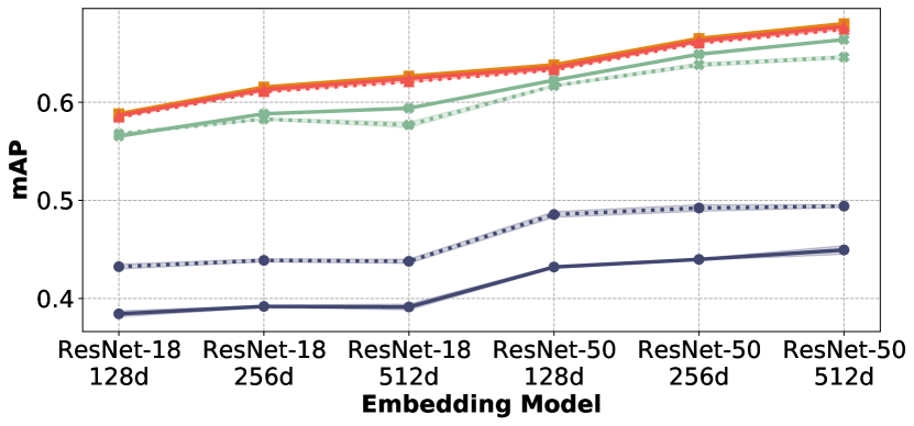
Figure 5: Active learning on ImageNet with varying embedding models (ResNet-18 or ResNet-50) and dimensions (128, 256, or 512). Performance increases with larger models and higher dimensional embeddings. However, SEALS achieves similar performance to the baseline approach regardless of the choice of model and dimension, empirically demonstrating SEALS’ robustness to the embedding function.

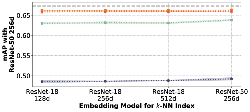
Figure 6: Active learning on ImageNet with 256-dimensional ResNet-50 embeddings and varying k-NN indices. Different embeddings might be used for learning rare concepts than the embeddings used for similarity search in practice. Fortunately, SEALS performs similarly for varying $k$-NN indices, as shown above. This can also be exploited to reduce further the cost of constructing the index by using a smaller, cheaper model to generate the embedding for similarity search and only applying the larger model to examples added to the candidate pool.

7.5 Impact of $k$ on SEALS

7.6 Impact of the number of initial positives on SEALS

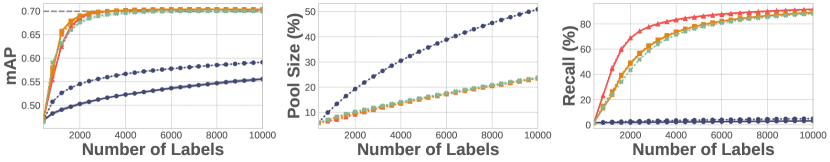
(a) ImageNet ($|U|$=639,906)

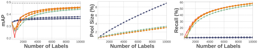
(b) OpenImages ($|U|$=6,816,296)

Figure 9: Active learning and search with 20 positive seed examples and a labeling budget of 10,000 examples on ImageNet (top) and OpenImages (bottom). Across datasets and strategies, SEALS with $k=100$ performs similarly to the baseline approach in terms of both the error the model achieves for active learning (left) and the recall of positive examples for active search (right), while only considering a fraction of the unlabeled data $U$ (middle).

(a) ImageNet ($|U|$=639,906)

(b) OpenImages ($|U|$=6,816,296)

Figure 10: Active learning and search with 50 positive seed examples and a labeling budget of 10,000 examples on ImageNet (top) and OpenImages (bottom). Across datasets and strategies, SEALS with $k=100$ performs similarly to the baseline approach in terms of both the error the model achieves for active learning (left) and the recall of positive examples for active search (right), while only considering a fraction of the unlabeled data $U$ (middle).

7.7 Latent structure

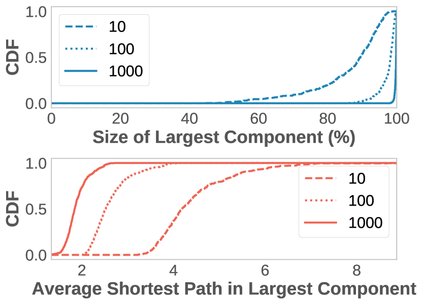
(a) ImageNet

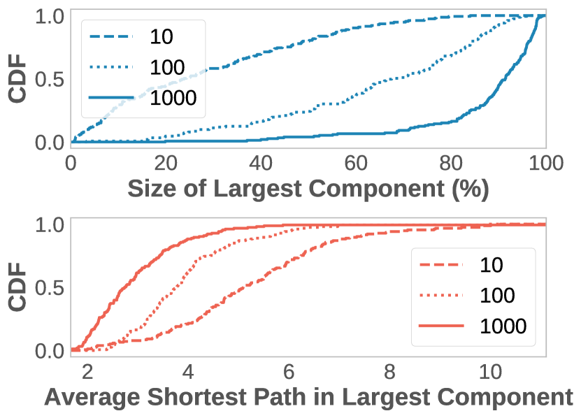
(b) OpenImages

Figure 11: Measurements of the latent structure of unseen concepts in ImageNet and OpenImages. The 10B images dataset was excluded because only a few thousand examples were labeled. The largest connected component gives a sense of how much of the concept SEALS can reach, while the average shortest path serves as a proxy for how long it will take to explore.

7.8 Comparison to pool of randomly selected examples

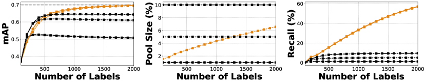
(a) ImageNet ($|U|$=639,906)

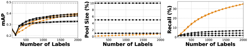
(b) OpenImages ($|U|$=6,816,296)

Figure 14: MaxEnt-SEALS ($k=100$) versus MaxEnt applied to a candidate pool of randomly selected examples (RandPool). Because the concepts we considered were so rare, as is often the case in practice, randomly chosen examples are unlikely to be close to the decision boundary, and a much larger pool is required to match SEALS. On ImageNet (top), MaxEnt-SEALS outperformed MaxEnt-RandPool in terms of both the error the model achieves for active learning (left) and the recall of positive examples for active search (right) even with a pool containing 10% of the data (middle). On Openimages (bottom), MaxEnt-RandPool needed at least $5\times$ as much data to match MaxEnt-SEALS for active learning and failed to achieve similar recall even with $10\times$ the data.

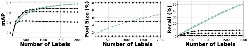
(a) ImageNet ($|U|$=639,906)

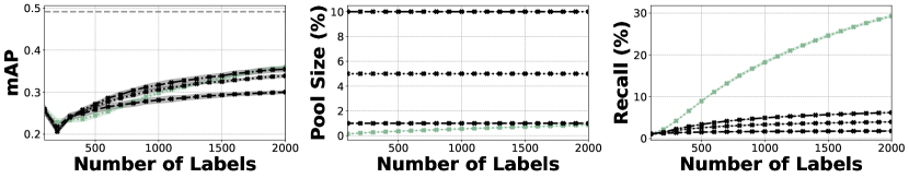
(b) OpenImages ($|U|$=6,816,296)

Figure 15: MLP-SEALS ($k=100$) versus MLP applied to a candidate pool of randomly selected examples (RandPool). Because the concepts we considered were so rare, as is often the case in practice, randomly chosen examples are unlikely to be close to the decision boundary, and a much larger pool is required to match SEALS. On ImageNet (top), MLP-SEALS outperformed MLP-RandPool in terms of both the error the model achieves for active learning (left) and the recall of positive examples for active search (right) even with a pool containing 10% of the data (middle). On Openimages (bottom), MLP-RandPool needed at least $5\times$ as much data to match MLP-SEALS for active learning and failed to achieve similar recall even with $10\times$ the data.

(a) ImageNet ($|U|$=639,906)

(b) OpenImages ($|U|$=6,816,296)

Figure 16: ID-SEALS ($k=100$) versus ID applied to a candidate pool of randomly selected examples (RandPool). Because the concepts we considered were so rare, as is often the case in practice, randomly chosen examples are unlikely to be close to the decision boundary, and a much larger pool is required to match SEALS. On ImageNet (top), ID-SEALS outperformed ID-RandPool in terms of both the error the model achieves for active learning (left) and the recall of positive examples for active search (right) even with a pool containing 10% of the data (middle). On Openimages (bottom), ID-RandPool needed at least $5\times$ as much data to match ID-SEALS for active learning and failed to achieve similar recall even with $10\times$ the data.

7.9 Active learning on each selected class from OpenImages

Table 3: Top $\frac{1}{3}$ of classes from Openimages for active learning. (1 of 3) Average precision and measurements of the largest component (LC) for each selected class (153 total) from OpenImages with a labeling budget of 2,000 examples. Classes are ordered based on MaxEnt-SEALS.

Display Name	Total Positives	Size of the LC (%)	Average Shortest Path in the LC	Random (All)	MaxEnt (SEALS)	MaxEnt (All)	Full Supervision
Citrus	796	65	3.34	$0.34$	$0.87$	$0.87$	$0.87$
Cargo ship	219	84	2.85	$0.70$	$0.83$	$0.83$	$0.86$
Blackberry	245	87	2.64	$0.67$	$0.80$	$0.80$	$0.79$
Galliformes	674	82	3.98	$0.72$	$0.80$	$0.82$	$0.92$
Rope	618	59	3.48	$0.29$	$0.80$	$0.81$	$0.74$
Hurdling	269	92	2.48	$0.26$	$0.80$	$0.79$	$0.80$
Roman temple	345	89	2.72	$0.63$	$0.79$	$0.79$	$0.82$
Monster truck	286	84	2.84	$0.41$	$0.79$	$0.80$	$0.81$
Pasta	954	91	3.21	$0.42$	$0.75$	$0.75$	$0.79$
Chess	740	83	3.39	$0.53$	$0.73$	$0.74$	$0.86$
Bowed string instrument	728	78	3.05	$0.72$	$0.72$	$0.74$	$0.79$
Parrot	1546	89	2.85	$0.59$	$0.72$	$0.76$	$0.92$
Calabaza	870	82	3.15	$0.50$	$0.71$	$0.75$	$0.81$
Superhero	968	58	5.28	$0.17$	$0.70$	$0.70$	$0.67$
Drums	741	69	3.30	$0.52$	$0.70$	$0.72$	$0.83$
Shooting range	189	57	3.06	$0.38$	$0.69$	$0.69$	$0.68$
Ancient roman architecture	589	76	3.34	$0.61$	$0.68$	$0.70$	$0.77$
Cupboard	898	88	3.41	$0.53$	$0.68$	$0.69$	$0.75$
Ibis	259	93	2.53	$0.29$	$0.68$	$0.69$	$0.66$
Cattle	5995	93	3.22	$0.37$	$0.67$	$0.68$	$0.74$
Galleon	182	74	2.54	$0.45$	$0.66$	$0.66$	$0.61$
Kitchen knife	360	63	3.52	$0.32$	$0.66$	$0.65$	$0.66$
Grapefruit	506	83	3.06	$0.50$	$0.65$	$0.65$	$0.69$
Deacon	341	80	2.80	$0.48$	$0.64$	$0.64$	$0.67$
Rye	128	75	2.63	$0.51$	$0.64$	$0.64$	$0.65$
Chartreux	147	91	2.59	$0.50$	$0.63$	$0.63$	$0.69$
San Pedro cactus	318	76	3.32	$0.17$	$0.62$	$0.63$	$0.71$
Skateboarding Equipment	862	57	5.92	$0.20$	$0.62$	$0.66$	$0.66$
Electric piano	345	56	4.15	$0.24$	$0.61$	$0.60$	$0.48$
Straw	547	65	2.85	$0.33$	$0.61$	$0.62$	$0.61$
Berry	874	82	3.78	$0.30$	$0.61$	$0.61$	$0.69$
East-european shepherd	206	86	2.16	$0.61$	$0.61$	$0.62$	$0.65$
Ring	676	75	3.87	$0.15$	$0.61$	$0.64$	$0.64$
Rat	1151	94	2.50	$0.32$	$0.60$	$0.60$	$0.61$
Coral reef fish	434	90	3.07	$0.51$	$0.60$	$0.64$	$0.79$
Concert dance	357	61	3.91	$0.37$	$0.60$	$0.60$	$0.70$
Whole food	708	73	3.66	$0.18$	$0.58$	$0.60$	$0.57$
Modern pentathlon	772	43	2.59	$0.13$	$0.58$	$0.47$	$0.51$
Gymnast	235	77	2.39	$0.39$	$0.57$	$0.59$	$0.65$
California roll	368	84	3.49	$0.05$	$0.56$	$0.56$	$0.58$
Shrimp	907	85	3.82	$0.07$	$0.56$	$0.56$	$0.58$
Log cabin	448	70	3.62	$0.44$	$0.55$	$0.55$	$0.62$
Formula racing	351	88	3.38	$0.33$	$0.55$	$0.54$	$0.60$
Herd	648	75	3.88	$0.42$	$0.54$	$0.55$	$0.67$
Embroidery	356	81	3.41	$0.32$	$0.53$	$0.53$	$0.60$
Shelving	810	66	3.41	$0.27$	$0.53$	$0.53$	$0.51$
Downhill	194	84	2.64	$0.42$	$0.53$	$0.51$	$0.59$
Daylily	391	87	3.25	$0.20$	$0.51$	$0.50$	$0.49$
Automotive exterior	1060	23	2.74	$0.65$	$0.49$	$0.54$	$0.69$
Ciconiiformes	426	88	3.47	$0.33$	$0.49$	$0.51$	$0.48$
Monoplane	756	81	4.70	$0.13$	$0.48$	$0.43$	$0.48$

Table 4: Middle $\frac{1}{3}$ of classes from Openimages for active learning. (2 of 3) Average precision and measurements of the largest component (LC) for each selected class (153 total) from OpenImages with a labeling budget of 2,000 examples. Classes are ordered based on MaxEnt-SEALS.

Display Name	Total Positives	Size of the LC (%)	Average Shortest Path in the LC	Random (All)	MaxEnt (SEALS)	MaxEnt (All)	Full Supervision
Seafood boil	322	85	2.73	$0.31$	$0.48$	$0.49$	$0.51$
Landscaping	789	32	4.71	$0.26$	$0.48$	$0.51$	$0.63$
Skating	561	77	4.04	$0.17$	$0.48$	$0.43$	$0.40$
Floodplain	567	50	4.81	$0.61$	$0.47$	$0.52$	$0.66$
Knitting	409	71	3.10	$0.61$	$0.46$	$0.50$	$0.73$
Elk	353	84	2.40	$0.15$	$0.46$	$0.48$	$0.45$
Bilberry	228	75	3.77	$0.10$	$0.45$	$0.45$	$0.32$
Goat	1190	88	3.72	$0.17$	$0.44$	$0.45$	$0.61$
Fortification	287	66	3.96	$0.43$	$0.44$	$0.46$	$0.52$
Annual plant	677	38	6.07	$0.39$	$0.44$	$0.43$	$0.58$
Mcdonnell douglas f/a-18 hornet	160	88	3.51	$0.11$	$0.44$	$0.47$	$0.37$
Tooth	976	49	4.77	$0.16$	$0.44$	$0.48$	$0.56$
Briefs	539	78	3.68	$0.15$	$0.43$	$0.44$	$0.46$
Sirloin steak	297	60	4.97	$0.14$	$0.42$	$0.42$	$0.46$
Smoothie	330	78	3.22	$0.15$	$0.41$	$0.41$	$0.38$
Glider	393	82	3.94	$0.08$	$0.40$	$0.40$	$0.48$
Bathroom cabinet	368	95	2.39	$0.29$	$0.40$	$0.39$	$0.37$
White-tailed deer	238	87	3.24	$0.34$	$0.40$	$0.43$	$0.43$
Bird of prey	712	78	3.81	$0.76$	$0.40$	$0.50$	$0.91$
Egg (Food)	1193	85	4.31	$0.14$	$0.40$	$0.37$	$0.63$
Soldier	1032	74	3.80	$0.62$	$0.40$	$0.41$	$0.72$
Cranberry	450	63	4.10	$0.13$	$0.39$	$0.39$	$0.37$
Estate	667	51	4.03	$0.47$	$0.39$	$0.40$	$0.54$
Chocolate truffle	288	58	5.47	$0.10$	$0.39$	$0.40$	$0.42$
Town square	617	58	3.69	$0.31$	$0.38$	$0.36$	$0.47$
Bakmi	191	76	3.34	$0.27$	$0.37$	$0.37$	$0.36$
Trail riding	679	90	3.15	$0.21$	$0.37$	$0.37$	$0.38$
Aerial photography	931	63	3.99	$0.39$	$0.37$	$0.37$	$0.66$
Lugger	103	62	3.14	$0.35$	$0.37$	$0.37$	$0.42$
Paddy field	468	70	4.02	$0.17$	$0.36$	$0.36$	$0.43$
Pavlova	195	86	2.60	$0.19$	$0.36$	$0.36$	$0.34$
Steamed rice	580	75	4.54	$0.10$	$0.35$	$0.37$	$0.48$
Pancit	385	86	3.16	$0.21$	$0.33$	$0.33$	$0.31$
Factory	333	61	5.59	$0.17$	$0.33$	$0.34$	$0.35$
Fur	834	42	4.31	$0.08$	$0.33$	$0.33$	$0.31$
Stallion	598	70	3.58	$0.32$	$0.33$	$0.40$	$0.64$
Optical instrument	649	79	3.91	$0.15$	$0.33$	$0.33$	$0.28$
Thumb	895	26	4.18	$0.07$	$0.32$	$0.39$	$0.41$
Meal	1250	60	5.68	$0.52$	$0.32$	$0.38$	$0.59$
American shorthair	2084	94	3.32	$0.12$	$0.32$	$0.32$	$0.24$
Bracelet	770	46	4.13	$0.09$	$0.31$	$0.33$	$0.24$
Vehicle registration plate	5697	76	5.89	$0.28$	$0.31$	$0.33$	$0.53$
Ice	682	50	4.87	$0.23$	$0.30$	$0.32$	$0.55$
Lamian	257	80	3.57	$0.23$	$0.29$	$0.32$	$0.28$
Multimedia	741	46	4.12	$0.45$	$0.29$	$0.31$	$0.53$
Belt	467	41	3.26	$0.06$	$0.29$	$0.31$	$0.31$
Prairie	792	44	3.92	$0.37$	$0.29$	$0.26$	$0.57$
Boardsport	673	62	4.08	$0.26$	$0.29$	$0.29$	$0.53$
Asphalt	1026	40	4.53	$0.23$	$0.29$	$0.29$	$0.45$
Costume design	818	52	3.44	$0.07$	$0.26$	$0.26$	$0.28$
Cottage	670	51	4.13	$0.36$	$0.26$	$0.36$	$0.61$

Table 5: Bottom $\frac{1}{3}$ of classes from Openimages for active learning. (3 of 3) Average precision and measurements of the largest component (LC) for each selected class (153 total) from OpenImages with a labeling budget of 2,000 examples. Classes are ordered based on MaxEnt-SEALS.

Display Name	Total Positives	Size of the LC (%)	Average Shortest Path in the LC	Random (All)	MaxEnt (SEALS)	MaxEnt (All)	Full Supervision
Stele	450	70	3.74	$0.12$	$0.26$	$0.25$	$0.35$
Mode of transport	1387	24	4.50	$0.15$	$0.26$	$0.16$	$0.54$
Temperate coniferous forest	328	59	4.23	$0.30$	$0.26$	$0.29$	$0.40$
Bumper	985	37	6.65	$0.49$	$0.25$	$0.38$	$0.64$
Interaction	924	15	6.05	$0.04$	$0.24$	$0.25$	$0.37$
Plumbing fixture	2124	89	3.19	$0.31$	$0.24$	$0.27$	$0.38$
Shorebird	234	80	2.76	$0.32$	$0.23$	$0.26$	$0.37$
Icing	1118	74	4.20	$0.13$	$0.23$	$0.25$	$0.46$
Wilderness	1225	30	4.12	$0.29$	$0.23$	$0.24$	$0.39$
Construction	515	63	4.99	$0.13$	$0.23$	$0.26$	$0.34$
Carpet	644	50	6.98	$0.05$	$0.23$	$0.28$	$0.43$
Maple	2301	90	4.19	$0.06$	$0.22$	$0.21$	$0.36$
Rural area	921	41	4.63	$0.33$	$0.22$	$0.28$	$0.50$
Singer	604	56	4.06	$0.12$	$0.21$	$0.21$	$0.40$
Delicatessen	196	52	2.80	$0.14$	$0.21$	$0.22$	$0.27$
Canal	726	62	4.78	$0.22$	$0.21$	$0.26$	$0.46$
Organ (Biology)	1156	25	3.80	$0.23$	$0.19$	$0.07$	$0.44$
Laugh	750	19	6.22	$0.06$	$0.18$	$0.17$	$0.26$
Plateau	452	37	3.88	$0.41$	$0.18$	$0.24$	$0.46$
Algae	426	57	4.52	$0.15$	$0.18$	$0.19$	$0.26$
Cactus	377	51	4.11	$0.05$	$0.17$	$0.18$	$0.22$
Engine	656	82	3.43	$0.16$	$0.17$	$0.17$	$0.26$
Marine mammal	2954	91	3.58	$0.19$	$0.16$	$0.15$	$0.21$
Frost	483	60	4.73	$0.20$	$0.15$	$0.21$	$0.47$
Paper	969	23	3.18	$0.16$	$0.15$	$0.14$	$0.41$
Cirque	347	29	5.77	$0.43$	$0.15$	$0.40$	$0.55$
Pork	464	64	4.44	$0.06$	$0.14$	$0.14$	$0.15$
Antenna	545	73	3.66	$0.10$	$0.14$	$0.13$	$0.29$
Portrait	2510	67	6.38	$0.23$	$0.13$	$0.18$	$0.43$
Flooring	814	38	3.87	$0.10$	$0.13$	$0.14$	$0.20$
Cycling	794	63	5.00	$0.53$	$0.13$	$0.28$	$0.66$
Chevrolet silverado	115	62	4.82	$0.05$	$0.09$	$0.08$	$0.12$
Tool	1549	64	4.51	$0.08$	$0.09$	$0.10$	$0.13$
Liqueur	539	51	5.98	$0.26$	$0.09$	$0.14$	$0.38$
Pleurotus eryngii	140	84	3.10	$0.11$	$0.08$	$0.08$	$0.14$
Organism	1148	21	3.49	$0.05$	$0.07$	$0.13$	$0.26$
Pelecaniformes	457	85	3.96	$0.30$	$0.07$	$0.09$	$0.32$
Icon	186	15	3.26	$0.05$	$0.07$	$0.07$	$0.16$
Stadium	1654	77	5.77	$0.35$	$0.06$	$0.10$	$0.48$
Space	1006	23	4.63	$0.03$	$0.06$	$0.03$	$0.14$
Performing arts	1030	29	6.97	$0.12$	$0.05$	$0.06$	$0.53$
Mural	649	41	5.24	$0.13$	$0.05$	$0.07$	$0.34$
Brown	1427	16	3.49	$0.02$	$0.05$	$0.07$	$0.20$
Wall	1218	27	3.13	$0.11$	$0.05$	$0.05$	$0.27$
Tournament	841	47	9.90	$0.15$	$0.05$	$0.07$	$0.16$
White	1494	3	2.79	$0.02$	$0.03$	$0.01$	$0.10$
Mitsubishi	511	37	5.14	$0.01$	$0.02$	$0.02$	$0.04$
Exhibition	513	40	3.87	$0.03$	$0.02$	$0.02$	$0.14$
Scale model	667	45	5.64	$0.05$	$0.02$	$0.02$	$0.13$
Teal	975	16	4.08	$0.01$	$0.01$	$0.01$	$0.04$
Electric blue	1180	19	3.70	$0.01$	$0.00$	$0.01$	$0.06$

7.10 Active search on each selected class from OpenImages

Table 6: Top $\frac{1}{3}$ of classes from Openimages for active search. (1 of 3) Recall (%) of positives and measurements of the largest component (LC) for each selected class (153 total) from OpenImages with a labeling budget of 2,000 examples. Classes are ordered based on MLP-SEALS.

Display Name	Total Positives	Size of the LC (%)	Average Shortest Path in the LC	Random (All)	MLP (SEALS)	MLP (All)
Chartreux	147	91	2.59	$3.5$	$83.9$	$84.6$
Ibis	259	93	2.53	$2.0$	$83.9$	$83.9$
Hurdling	269	92	2.48	$1.9$	$83.5$	$86.2$
East-european shepherd	206	86	2.16	$2.4$	$78.2$	$78.3$
Blackberry	245	87	2.64	$2.0$	$77.5$	$78.5$
Bathroom cabinet	368	95	2.39	$1.4$	$76.8$	$77.1$
Rat	1151	94	2.50	$0.5$	$75.1$	$75.2$
Rye	128	75	2.63	$3.9$	$74.7$	$74.5$
Elk	353	84	2.40	$1.5$	$73.4$	$74.3$
Pavlova	195	86	2.60	$2.6$	$70.8$	$71.3$
Seafood boil	322	85	2.73	$1.6$	$70.4$	$70.6$
Roman temple	345	89	2.72	$1.5$	$69.2$	$68.3$
Monster truck	286	84	2.84	$1.7$	$68.1$	$67.8$
Downhill	194	84	2.64	$2.6$	$67.2$	$69.0$
Shorebird	234	80	2.76	$2.1$	$66.8$	$66.4$
Mcdonnell douglas f/a-18 hornet	160	88	3.51	$3.2$	$66.0$	$67.9$
San Pedro cactus	318	76	3.32	$1.6$	$65.8$	$64.9$
Pleurotus eryngii	140	84	3.10	$3.6$	$65.7$	$66.1$
California roll	368	84	3.49	$1.4$	$65.3$	$68.0$
Gymnast	235	77	2.39	$2.2$	$64.0$	$64.0$
Galleon	182	74	2.54	$2.7$	$62.4$	$61.5$
Cargo ship	219	84	2.85	$2.3$	$61.1$	$61.7$
Trail riding	679	90	3.15	$0.8$	$59.7$	$60.7$
Daylily	391	87	3.25	$1.3$	$59.4$	$59.5$
Grapefruit	506	83	3.06	$1.0$	$59.4$	$60.4$
Bilberry	228	75	3.77	$2.2$	$58.9$	$55.2$
Smoothie	330	78	3.22	$1.5$	$58.0$	$59.8$
Embroidery	356	81	3.41	$1.5$	$57.6$	$57.2$
Deacon	341	80	2.80	$1.5$	$57.1$	$57.9$
Shooting range	189	57	3.06	$2.6$	$56.3$	$55.6$
Glider	393	82	3.94	$1.3$	$55.8$	$57.6$
White-tailed deer	238	87	3.24	$2.2$	$55.8$	$55.9$
Coral reef fish	434	90	3.07	$1.3$	$54.8$	$54.9$
Chevrolet silverado	115	62	4.82	$4.3$	$54.1$	$54.6$
Lugger	103	62	3.14	$4.9$	$53.8$	$53.8$
Pancit	385	86	3.16	$1.3$	$52.8$	$53.1$
Chess	740	83	3.39	$0.7$	$51.9$	$50.9$
Bakmi	191	76	3.34	$2.6$	$51.8$	$51.2$
Kitchen knife	360	63	3.52	$1.5$	$50.9$	$53.9$
Straw	547	65	2.85	$1.0$	$50.3$	$51.0$
Ancient roman architecture	589	76	3.34	$0.8$	$48.5$	$47.1$
Lamian	257	80	3.57	$1.9$	$47.8$	$48.2$
Antenna	545	73	3.66	$1.0$	$47.4$	$48.0$
Calabaza	870	82	3.15	$0.6$	$46.0$	$45.8$
Ring	676	75	3.87	$0.7$	$45.2$	$45.4$
Ciconiiformes	426	88	3.47	$1.2$	$45.2$	$45.2$
Log cabin	448	70	3.62	$1.1$	$44.9$	$45.7$
Bowed string instrument	728	78	3.05	$0.7$	$44.4$	$44.7$
Pasta	954	91	3.21	$0.5$	$43.7$	$43.8$
Knitting	409	71	3.10	$1.3$	$43.5$	$42.8$
Rope	618	59	3.48	$0.8$	$43.0$	$42.8$

Table 7: Middle $\frac{1}{3}$ of classes from Openimages for active search. (2 of 3) Recall (%) of positives and measurements of the largest component (LC) for each selected class (153 total) from OpenImages with a labeling budget of 2,000 examples. Classes are ordered based on MLP-SEALS.

Display Name	Total Positives	Size of the LC (%)	Average Shortest Path in the LC	Random (All)	MLP (SEALS)	MLP (All)
Formula racing	351	88	3.38	$1.4$	$42.6$	$41.4$
Paddy field	468	70	4.02	$1.1$	$42.6$	$44.2$
Engine	656	82	3.43	$0.8$	$41.7$	$40.6$
Electric piano	345	56	4.15	$1.5$	$40.9$	$42.1$
Shrimp	907	85	3.82	$0.6$	$40.4$	$40.8$
Goat	1190	88	3.72	$0.4$	$39.6$	$39.6$
Chocolate truffle	288	58	5.47	$1.8$	$39.6$	$39.9$
Cupboard	898	88	3.41	$0.6$	$39.6$	$39.6$
Citrus	796	65	3.34	$0.7$	$39.3$	$39.6$
Parrot	1546	89	2.85	$0.4$	$39.2$	$38.8$
Delicatessen	196	52	2.80	$2.6$	$38.2$	$39.0$
Berry	874	82	3.78	$0.6$	$37.8$	$37.6$
Briefs	539	78	3.68	$1.0$	$37.1$	$37.2$
Concert dance	357	61	3.91	$1.4$	$36.6$	$36.1$
Modern pentathlon	772	43	2.59	$0.6$	$35.9$	$32.6$
Fortification	287	66	3.96	$1.7$	$35.7$	$37.6$
Stallion	598	70	3.58	$0.9$	$35.7$	$36.3$
Belt	467	41	3.26	$1.1$	$35.2$	$34.9$
Sirloin steak	297	60	4.97	$1.8$	$33.9$	$32.7$
Stele	450	70	3.74	$1.1$	$33.9$	$32.7$
Galliformes	674	82	3.98	$0.7$	$33.9$	$33.9$
Algae	426	57	4.52	$1.2$	$33.8$	$33.1$
Herd	648	75	3.88	$0.8$	$33.5$	$33.7$
Pelecaniformes	457	85	3.96	$1.1$	$33.4$	$37.5$
Cactus	377	51	4.11	$1.3$	$33.4$	$35.2$
Shelving	810	66	3.41	$0.7$	$33.2$	$33.3$
Drums	741	69	3.30	$0.7$	$32.9$	$32.7$
Cranberry	450	63	4.10	$1.2$	$32.9$	$33.7$
Factory	333	61	5.59	$1.5$	$32.0$	$31.7$
Costume design	818	52	3.44	$0.6$	$30.9$	$30.6$
Optical instrument	649	79	3.91	$0.8$	$30.3$	$32.8$
Construction	515	63	4.99	$1.0$	$30.1$	$31.1$
Temperate coniferous forest	328	59	4.23	$1.5$	$30.1$	$27.6$
Skating	561	77	4.04	$1.0$	$28.8$	$30.4$
Egg (Food)	1193	85	4.31	$0.4$	$28.8$	$28.6$
Steamed rice	580	75	4.54	$0.9$	$28.1$	$30.2$
Plumbing fixture	2124	89	3.19	$0.3$	$27.9$	$27.9$
Whole food	708	73	3.66	$0.7$	$27.7$	$27.5$
Boardsport	673	62	4.08	$0.8$	$26.8$	$26.5$
Pork	464	64	4.44	$1.1$	$26.3$	$26.6$
Aerial photography	931	63	3.99	$0.6$	$25.8$	$26.1$
Town square	617	58	3.69	$0.8$	$25.7$	$26.1$
Estate	667	51	4.03	$0.9$	$24.8$	$25.9$
Maple	2301	90	4.19	$0.2$	$24.3$	$24.4$
Cattle	5995	93	3.22	$0.1$	$23.8$	$23.6$
Superhero	968	58	5.28	$0.6$	$23.4$	$23.3$
Bracelet	770	46	4.13	$0.6$	$23.2$	$24.8$
Frost	483	60	4.73	$1.0$	$23.1$	$22.5$
Scale model	667	45	5.64	$0.8$	$22.9$	$23.7$
Plateau	452	37	3.88	$1.1$	$22.7$	$19.1$
Bird of prey	712	78	3.81	$0.7$	$22.4$	$22.0$

Table 8: Bottom $\frac{1}{3}$ of classes from Openimages for active search. (3 of 3) Recall (%) of positives and measurements of the largest component (LC) for each selected class (153 total) from OpenImages with a labeling budget of 2,000 examples. Classes are ordered based on MLP-SEALS.

Display Name	Total Positives	Size of the LC (%)	Average Shortest Path in the LC	Random (All)	MLP (SEALS)	MLP (All)
Canal	726	62	4.78	$0.7$	$22.4$	$20.9$
Exhibition	513	40	3.87	$1.0$	$21.9$	$23.1$
Carpet	644	50	6.98	$0.8$	$21.9$	$22.7$
Monoplane	756	81	4.70	$0.7$	$21.8$	$20.1$
Ice	682	50	4.87	$0.8$	$21.6$	$23.1$
Fur	834	42	4.31	$0.6$	$21.2$	$17.3$
Icing	1118	74	4.20	$0.4$	$20.5$	$20.1$
Flooring	814	38	3.87	$0.6$	$20.4$	$16.9$
Icon	186	15	3.26	$2.7$	$19.9$	$17.2$
Prairie	792	44	3.92	$0.6$	$19.0$	$19.2$
Tooth	976	49	4.77	$0.5$	$18.6$	$18.0$
Skateboarding Equipment	862	57	5.92	$0.6$	$18.1$	$19.3$
Automotive exterior	1060	23	2.74	$0.5$	$17.7$	$11.9$
Cottage	670	51	4.13	$0.7$	$17.6$	$17.3$
Soldier	1032	74	3.80	$0.5$	$17.3$	$16.8$
Marine mammal	2954	91	3.58	$0.2$	$17.3$	$17.2$
Tool	1549	64	4.51	$0.3$	$17.0$	$16.9$
Multimedia	741	46	4.12	$0.7$	$16.8$	$17.1$
American shorthair	2084	94	3.32	$0.3$	$16.5$	$16.7$
Asphalt	1026	40	4.53	$0.5$	$15.1$	$11.5$
Singer	604	56	4.06	$0.9$	$14.6$	$13.6$
Floodplain	567	50	4.81	$0.9$	$14.6$	$14.0$
Rural area	921	41	4.63	$0.6$	$14.2$	$13.2$
Mitsubishi	511	37	5.14	$1.0$	$12.6$	$11.8$
Organ (Biology)	1156	25	3.80	$0.5$	$12.1$	$15.9$
Paper	969	23	3.18	$0.5$	$12.0$	$14.8$
Annual plant	677	38	6.07	$0.7$	$11.8$	$10.7$
Electric blue	1180	19	3.70	$0.5$	$11.5$	$9.4$
Stadium	1654	77	5.77	$0.3$	$10.8$	$9.3$
Mural	649	41	5.24	$0.8$	$10.4$	$10.3$
Teal	975	16	4.08	$0.5$	$9.9$	$10.4$
Cirque	347	29	5.77	$1.5$	$9.9$	$9.8$
Wall	1218	27	3.13	$0.4$	$9.3$	$12.0$
Thumb	895	26	4.18	$0.6$	$9.3$	$13.8$
Landscaping	789	32	4.71	$0.7$	$9.2$	$9.3$
Vehicle registration plate	5697	76	5.89	$0.1$	$8.7$	$8.3$
Meal	1250	60	5.68	$0.4$	$8.5$	$9.1$
Wilderness	1225	30	4.12	$0.4$	$8.5$	$9.8$
Liqueur	539	51	5.98	$1.0$	$8.0$	$12.8$
Space	1006	23	4.63	$0.5$	$7.8$	$6.3$
Cycling	794	63	5.00	$0.6$	$7.3$	$7.8$
Brown	1427	16	3.49	$0.4$	$7.2$	$2.6$
Organism	1148	21	3.49	$0.4$	$6.8$	$2.0$
Laugh	750	19	6.22	$0.7$	$6.6$	$8.6$
Bumper	985	37	6.65	$0.5$	$5.9$	$8.3$
Portrait	2510	67	6.38	$0.2$	$5.8$	$5.3$
Mode of transport	1387	24	4.50	$0.4$	$5.1$	$3.6$
Interaction	924	15	6.05	$0.6$	$4.5$	$4.6$
Tournament	841	47	9.90	$0.6$	$4.3$	$5.1$
Performing arts	1030	29	6.97	$0.5$	$2.3$	$2.5$
White	1494	3	2.79	$0.3$	$2.0$	$0.5$

7.11 Self-supervised embeddings (SimCLR) on ImageNet

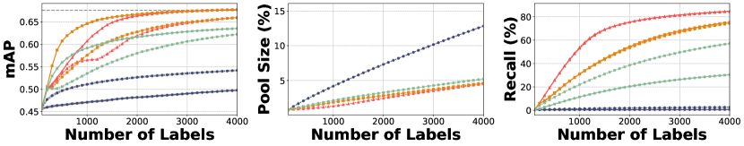
Figure 17: Active learning and search on ImageNet with self-supervised embeddings from SimCLR [11]. Because the self-supervised training for the embeddings did not use the labels, results are average across all 1,000 classes and $|U|$=1,281,167. To compensate for the larger unlabeled pool, we extended the total labeling budget to 4,000 compared to the 2,000 used in Figure 1. Across strategies, SEALS with $k=100$ substantially outperforms random sampling in terms of both the mAP the model achieves for active learning (left) and the recall of positive examples for active search (right), while only considering a fraction of the data $U$ (middle). For active learning, the gap between the baseline and SEALS approaches is slightly larger than in Figure 1, which is likely due to the larger pool size and increased average shortest paths (see Figure 18).

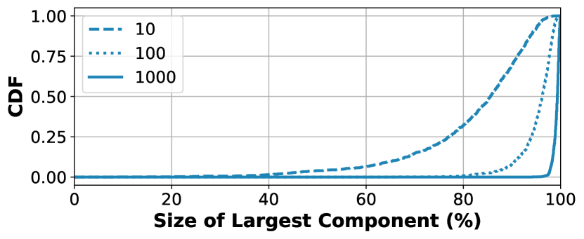
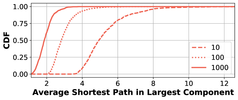
Figure 18: Measurements of the latent structure of unseen concepts in ImageNet with self-supervised embeddings from SimCLR [11]. In comparison to Figure 11(a), the $k$-nearest neighbor graph for unseen concepts was still well connected, forming large connected components (left) for even moderate values of $k$, but the average shortest path between examples was slightly longer (right). The increased path length is not too surprising considering the fully supervised model still outperformed the linear evaluation of the self-supervised embeddings in Chen et al. [11].

7.12 Self-supervised embedding (Sentence-BERT) on Goodreads

We followed the same general procedure described in Section 5.1, aside from the dataset specific details below. Goodreads spoiler detection [46] had 17.67 million sentences with binary spoiler annotations. Spoilers made up 3.224% of the data, making them much more common than the rare concepts we evaluated in the other datasets. Following Wan et al. [46], we used 3.53 million sentences for testing (20%), 10,000 sentences as the validation set, and the remaining 14.13 million sentences as the unlabeled pool. We also switched to the area under the ROC curve (AUC) as our primary evaluation metric for active learning to be consistent with Wan et al. [46]. For $G_{z}$, we used a pre-trained Sentence-BERT model (SBERT-NLI-base) [36], applied PCA whitening to reduce the dimension to 256, and performed $l^{2}$ normalization.

7.12.1 Active search

SEALS achieved the same recall as the baseline approaches, but only considered less than 1% of the unlabeled data in the candidate pool, as shown in Figure 19. At a labeling budget of 2,000, MLP-ALL and MLP-SEALS recalled $0.15\pm 0.02$% and $0.17\pm 0.05$%, respectively, while MaxEnt-All and MaxEnt-SEALS achieved $0.14\pm 0.04$% and $0.11\pm 0.06$% recall respectively. Increasing the labeling budget to 50,000 examples, increased recall to ~3.7% for MaxEnt and MLP but maintained a similar relative improvement over random sampling, as shown in Figure 20. ID-SEALS performed worse than the other strategies. However, all of the active selection strategies outperformed random sampling by up to an order of magnitude.

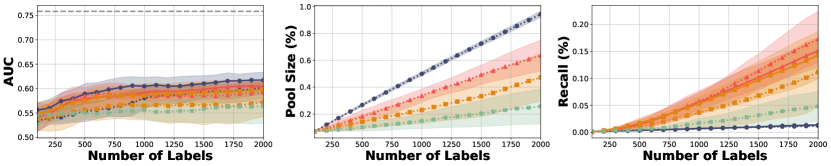
Figure 19: Active learning and search on Goodreads with Sentence-BERT embeddings. Across datasets and strategies, SEALS with $k=100$ performs similarly to the baseline approach in terms of both the error the model achieves for active learning (left) and the recall of positive examples for active search (right), while only considering a fraction of the data $U$ (middle).

7.12.2 Active learning

At a labeling budget of 2,000 examples, all the selection strategies were indistinguishable from random sampling. Increasing the labeling budget did not help, as shown in Figure 20. Unlike ImageNet and OpenImages, Goodreads had a much higher fraction of positive examples (3.224%), and the examples were not tightly clustered as described in Section 7.12.3.

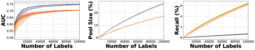
Figure 20: Active learning and search on Goodreads with a labeling budget of 100,000 examples. Across strategies, SEALS with $k=100$ performed similarly to the baseline approach in terms of both the error the model achieved for active learning (left) and the recall of positive examples for active search (right), while only considering a fraction of the data $U$ (middle). ID was excluded because of the growing pool size and computation. For active search, MaxEnt and MLP continued to improve recall. For active learning, all the selection strategies (both with and without SEALS) performed worse than random sampling despite the larger labeling budget. This gap was likely due to spoilers being book specific and the higher fraction of positive examples in the unlabeled pool, causing relevant examples to be spread almost uniformly across the space (see Section 7.12.3).

7.12.3 Latent structure

The large number of positive examples in the Goodreads dataset limited the analysis we could perform. We could only calculate the size of the largest connected component in the nearest neighbor graph (Figure 21). For $k=10$, only 28.4% of the positive examples could be reached directly, but increasing $k$ to 100 improved that dramatically to 96.7%. For such a large connected component, one might have expected active learning to perform better in Section 7.12.2. By analyzing the embeddings, however, we found that examples are spread almost uniformly across the space with an average cosine similarity of 0.004. For comparison, the average cosine similarity for concepts in ImageNet and OpenImages was $0.453\pm 0.077$ and $0.361\pm 0.105$ respectively. This uniformity was likely due to the higher fraction of positive examples and spoilers being book specific while Sentence-BERT is trained on generic data. As a result, even if spoilers were tightly clustered within each book, the books were spread across a range of topics and consequently across the embedding space, illustrating a limitation and opportunity for future work.

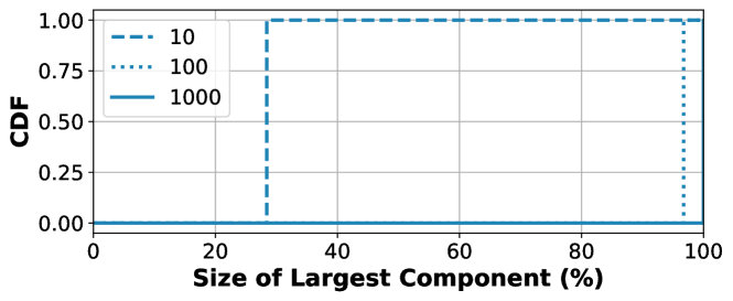
Figure 21: Cumulative distribution function (CDF) for the largest connected component in the Goodreads dataset with varying values of $k$.

References

- Abu-El-Haija et al. [2016] Sami Abu-El-Haija, Nisarg Kothari, Joonseok Lee, Paul Natsev, George Toderici, Balakrishnan Varadarajan, and Sudheendra Vijayanarasimhan. Youtube-8m: A large-scale video classification benchmark, 2016.
- Amodei and Hernandez [2018] Dario Amodei and Danny Hernandez. Ai and compute, May 2018. URL https://blog.openai.com/ai-and-compute/.
- Ashmawy et al. [2019] Khalid Ashmawy, Shouheng Yi, and Alex Chao. Searchable ground truth: Querying uncommon scenarios in self-driving car development. https://eng.uber.com/searchable-ground-truth-atg/, 10 2019.
- Babenko and Lempitsky [2016] Artem Babenko and Victor Lempitsky. Efficient indexing of billion-scale datasets of deep descriptors. In Proceedings of the IEEE Conference on Computer Vision and Pattern Recognition, pages 2055–2063, 2016.
- Babenko et al. [2014] Artem Babenko, Anton Slesarev, Alexandr Chigorin, and Victor Lempitsky. Neural codes for image retrieval. In European conference on computer vision, pages 584–599. Springer, 2014.
- Balcan and Long [2013] Maria-Florina Balcan and Phil Long. Active and passive learning of linear separators under log-concave distributions. In Conference on Learning Theory, pages 288–316. PMLR, 2013.
- Beluch et al. [2018] William H Beluch, Tim Genewein, Andreas Nürnberger, and Jan M Köhler. The power of ensembles for active learning in image classification. In Proceedings of the IEEE Conference on Computer Vision and Pattern Recognition, pages 9368–9377, 2018.
- Boyd et al. [2004] Stephen Boyd, Stephen P Boyd, and Lieven Vandenberghe. Convex optimization. Cambridge university press, 2004.
- Charikar [2002] Moses S Charikar. Similarity estimation techniques from rounding algorithms. In Proceedings of the thiry-fourth annual ACM symposium on Theory of computing, pages 380–388, 2002.
- Chelba et al. [2013] Ciprian Chelba, Tomas Mikolov, Mike Schuster, Qi Ge, Thorsten Brants, Phillipp Koehn, and Tony Robinson. One billion word benchmark for measuring progress in statistical language modeling. Technical report, Google, 2013. URL http://arxiv.org/abs/1312.3005.
- Chen et al. [2020] Ting Chen, Simon Kornblith, Mohammad Norouzi, and Geoffrey Hinton. A simple framework for contrastive learning of visual representations. arXiv preprint arXiv:2002.05709, 2020.
- Coleman et al. [2020] Cody Coleman, Christopher Yeh, Stephen Mussmann, Baharan Mirzasoleiman, Peter Bailis, Percy Liang, Jure Leskovec, and Matei Zaharia. Selection via proxy: Efficient data selection for deep learning. In International Conference on Learning Representations, 2020. URL https://openreview.net/forum?id=HJg2b0VYDr.
- Ertekin et al. [2007] Seyda Ertekin, Jian Huang, Leon Bottou, and Lee Giles. Learning on the border: active learning in imbalanced data classification. In Proceedings of the sixteenth ACM conference on Conference on information and knowledge management, pages 127–136, 2007.
- Gal et al. [2017] Yarin Gal, Riashat Islam, and Zoubin Ghahramani. Deep Bayesian active learning with image data. In Doina Precup and Yee Whye Teh, editors, Proceedings of the 34th International Conference on Machine Learning, volume 70 of Proceedings of Machine Learning Research, pages 1183–1192. PMLR, 06–11 Aug 2017. URL http://proceedings.mlr.press/v70/gal17a.html.
- Garnett et al. [2012] Roman Garnett, Yamuna Krishnamurthy, Xuehan Xiong, Jeff Schneider, and Richard Mann. Bayesian optimal active search and surveying. In Proceedings of the 29th International Coference on International Conference on Machine Learning, ICML’12, page 843–850, Madison, WI, USA, 2012. Omnipress. ISBN 9781450312851.
- He and Carbonell [2007] Jingrui He and Jaime G Carbonell. Nearest-neighbor-based active learning for rare category detection. 2007.
- He et al. [2016] Kaiming He, Xiangyu Zhang, Shaoqing Ren, and Jian Sun. Deep residual learning for image recognition. In Proceedings of Conference on Computer Vision and Pattern Recognition, 2016.
- Holstein et al. [2019] Kenneth Holstein, Jennifer Wortman Vaughan, Hal Daumé III, Miro Dudik, and Hanna Wallach. Improving fairness in machine learning systems: What do industry practitioners need? In Proceedings of the 2019 CHI Conference on Human Factors in Computing Systems, pages 1–16, 2019.
- Jain et al. [2010] Prateek Jain, Sudheendra Vijayanarasimhan, and Kristen Grauman. Hashing hyperplane queries to near points with applications to large-scale active learning. Advances in Neural Information Processing Systems, 23:928–936, 2010.
- Jiang et al. [2017] Shali Jiang, Gustavo Malkomes, Geoff Converse, Alyssa Shofner, Benjamin Moseley, and Roman Garnett. Efficient nonmyopic active search. In Doina Precup and Yee Whye Teh, editors, Proceedings of the 34th International Conference on Machine Learning, volume 70 of Proceedings of Machine Learning Research, pages 1714–1723, International Convention Centre, Sydney, Australia, 06–11 Aug 2017. PMLR. URL http://proceedings.mlr.press/v70/jiang17d.html.
- Jiang et al. [2018] Shali Jiang, Gustavo Malkomes, Matthew Abbott, Benjamin Moseley, and Roman Garnett. Efficient nonmyopic batch active search. In Advances in Neural Information Processing Systems, pages 1099–1109, 2018.
- Jiang et al. [2019] Shali Jiang, Roman Garnett, and Benjamin Moseley. Cost effective active search. In H. Wallach, H. Larochelle, A. Beygelzimer, F. d'Alché-Buc, E. Fox, and R. Garnett, editors, Advances in Neural Information Processing Systems 32, pages 4880–4889. Curran Associates, Inc., 2019. URL http://papers.nips.cc/paper/8734-cost-effective-active-search.pdf.
- Johnson et al. [2017] Jeff Johnson, Matthijs Douze, and Hervé Jégou. Billion-scale similarity search with gpus. arXiv preprint arXiv:1702.08734, 2017.
- Joshi et al. [2009] Ajay J Joshi, Fatih Porikli, and Nikolaos Papanikolopoulos. Multi-class active learning for image classification. In 2009 IEEE Conference on Computer Vision and Pattern Recognition, pages 2372–2379. IEEE, 2009.
- Joshi et al. [2012] Ajay J Joshi, Fatih Porikli, and Nikolaos Papanikolopoulos. Coverage optimized active learning for k-nn classifiers. In 2012 IEEE International Conference on Robotics and Automation, pages 5353–5358. IEEE, 2012.
- Karpathy [2018] Andrej Karpathy. Train ai 2018 - building the software 2.0 stack, 2018. URL https://vimeo.com/272696002.
- Karpathy [2020] Andrej Karpathy. Ai for full-self driving, 2020. URL https://youtu.be/hx7BXih7zx8.
- Kirsch et al. [2019] Andreas Kirsch, Joost van Amersfoort, and Yarin Gal. Batchbald: Efficient and diverse batch acquisition for deep bayesian active learning. In Advances in Neural Information Processing Systems, pages 7024–7035, 2019.
- Kuznetsova et al. [2020] Alina Kuznetsova, Hassan Rom, Neil Alldrin, Jasper Uijlings, Ivan Krasin, Jordi Pont-Tuset, Shahab Kamali, Stefan Popov, Matteo Malloci, Alexander Kolesnikov, Tom Duerig, and Vittorio Ferrari. The open images dataset v4: Unified image classification, object detection, and visual relationship detection at scale. IJCV, 2020.
- Lee et al. [2019] Kevin Lee, Vijay Rao, and William Christie Arnold. Accelerating facebook’s infrastructure with application-specific hardware. https://engineering.fb.com/data-center-engineering/accelerating-infrastructure/, 3 2019.
- Lewis and Gale [1994] David D Lewis and William A Gale. A sequential algorithm for training text classifiers. In Proceedings of the 17th annual international ACM SIGIR conference on Research and development in information retrieval, pages 3–12. Springer-Verlag New York, Inc., 1994.
- Lin et al. [2018] Christopher Lin, Mausam Mausam, and Daniel Weld. Active learning with unbalanced classes and example-generation queries. In Proceedings of the AAAI Conference on Human Computation and Crowdsourcing, volume 6, 2018.
- Liu et al. [2019] Ziwei Liu, Zhongqi Miao, Xiaohang Zhan, Jiayun Wang, Boqing Gong, and Stella X Yu. Large-scale long-tailed recognition in an open world. In Proceedings of the IEEE Conference on Computer Vision and Pattern Recognition, pages 2537–2546, 2019.
- Mayer and Timofte [2020] Christoph Mayer and Radu Timofte. Adversarial sampling for active learning. In The IEEE Winter Conference on Applications of Computer Vision, pages 3071–3079, 2020.
- Pinsler et al. [2019] Robert Pinsler, Jonathan Gordon, Eric Nalisnick, and José Miguel Hernández-Lobato. Bayesian batch active learning as sparse subset approximation. In Advances in Neural Information Processing Systems, pages 6356–6367, 2019.
- Reimers and Gurevych [2019] Nils Reimers and Iryna Gurevych. Sentence-BERT: Sentence embeddings using Siamese BERT-networks. In Proceedings of the 2019 Conference on Empirical Methods in Natural Language Processing and the 9th International Joint Conference on Natural Language Processing (EMNLP-IJCNLP), pages 3982–3992, Hong Kong, China, November 2019. Association for Computational Linguistics. doi: 10.18653/v1/D19-1410. URL https://www.aclweb.org/anthology/D19-1410.
- Russakovsky et al. [2015] Olga Russakovsky, Jia Deng, Hao Su, Jonathan Krause, Sanjeev Satheesh, Sean Ma, Zhiheng Huang, Andrej Karpathy, Aditya Khosla, Michael Bernstein, et al. Imagenet large scale visual recognition challenge. International journal of computer vision, 115(3):211–252, 2015.
- Sener and Savarese [2018] Ozan Sener and Silvio Savarese. Active learning for convolutional neural networks: A core-set approach. In International Conference on Learning Representations, 2018. URL https://openreview.net/forum?id=H1aIuk-RW.
- Settles [2009] Burr Settles. Active learning literature survey. Technical report, University of Wisconsin-Madison Department of Computer Sciences, 2009.
- Settles [2011] Burr Settles. From theories to queries: Active learning in practice. In Isabelle Guyon, Gavin Cawley, Gideon Dror, Vincent Lemaire, and Alexander Statnikov, editors, Active Learning and Experimental Design workshop In conjunction with AISTATS 2010, volume 16 of Proceedings of Machine Learning Research, pages 1–18, Sardinia, Italy, 16 May 2011. PMLR. URL http://proceedings.mlr.press/v16/settles11a.html.
- Settles [2012] Burr Settles. Active learning. Synthesis Lectures on Artificial Intelligence and Machine Learning, 6(1):1–114, 2012.
- Settles and Craven [2008] Burr Settles and Mark Craven. An analysis of active learning strategies for sequence labeling tasks. In Proceedings of the Conference on Empirical Methods in Natural Language Processing, EMNLP ’08, page 1070–1079, USA, 2008. Association for Computational Linguistics.
- Sinha et al. [2019] Samarth Sinha, Sayna Ebrahimi, and Trevor Darrell. Variational adversarial active learning. In Proceedings of the IEEE/CVF International Conference on Computer Vision, pages 5972–5981, 2019.
- Thomee et al. [2016] Bart Thomee, David A. Shamma, Gerald Friedland, Benjamin Elizalde, Karl Ni, Douglas Poland, Damian Borth, and Li-Jia Li. Yfcc100m. Communications of the ACM, 59(2):64–73, Jan 2016. ISSN 1557-7317. doi: 10.1145/2812802. URL http://dx.doi.org/10.1145/2812802.
- Van Horn and Perona [2017] Grant Van Horn and Pietro Perona. The devil is in the tails: Fine-grained classification in the wild. arXiv preprint arXiv:1709.01450, 2017.
- Wan et al. [2019] Mengting Wan, Rishabh Misra, Ndapa Nakashole, and Julian J. McAuley. Fine-grained spoiler detection from large-scale review corpora. In Anna Korhonen, David R. Traum, and Lluís Màrquez, editors, Proceedings of the 57th Conference of the Association for Computational Linguistics, ACL 2019, Florence, Italy, July 28- August 2, 2019, Volume 1: Long Papers, pages 2605–2610. Association for Computational Linguistics, 2019. doi: 10.18653/v1/p19-1248. URL https://doi.org/10.18653/v1/p19-1248.
- Wang et al. [2017] Yu-Xiong Wang, Deva Ramanan, and Martial Hebert. Learning to model the tail. In Advances in Neural Information Processing Systems, pages 7029–7039, 2017.
- Warmuth et al. [2003] Manfred K Warmuth, Jun Liao, Gunnar Rätsch, Michael Mathieson, Santosh Putta, and Christian Lemmen. Active learning with support vector machines in the drug discovery process. Journal of chemical information and computer sciences, 43(2):667–673, 2003.
- Warmuth et al. [2002] Manfred KK Warmuth, Gunnar Rätsch, Michael Mathieson, Jun Liao, and Christian Lemmen. Active learning in the drug discovery process. In Advances in Neural information processing systems, pages 1449–1456, 2002.
- Wei et al. [2015] Kai Wei, Rishabh Iyer, and Jeff Bilmes. Submodularity in data subset selection and active learning. In International Conference on Machine Learning, pages 1954–1963, 2015.
- Yoo and Kweon [2019] Donggeun Yoo and In So Kweon. Learning loss for active learning. In Proceedings of the IEEE Conference on Computer Vision and Pattern Recognition, pages 93–102, 2019.
- Zhang et al. [2020] Beichen Zhang, Liang Li, Shijie Yang, Shuhui Wang, Zheng-Jun Zha, and Qingming Huang. State-relabeling adversarial active learning. In Proceedings of the IEEE/CVF Conference on Computer Vision and Pattern Recognition, pages 8756–8765, 2020.
- Zhang et al. [2015] Xiang Zhang, Junbo Zhao, and Yann LeCun. Character-level convolutional networks for text classification. In Advances in neural information processing systems, pages 649–657, 2015.
- Zhang et al. [2017] Xiao Zhang, Zhiyuan Fang, Yandong Wen, Zhifeng Li, and Yu Qiao. Range loss for deep face recognition with long-tailed training data. In Proceedings of the IEEE International Conference on Computer Vision, pages 5409–5418, 2017.
- Zhu and Bento [2017] Jia-Jie Zhu and José Bento. Generative adversarial active learning. arXiv preprint arXiv:1702.07956, 2017.