A Reinforcement Learning Approach for Dynamic Information Flow Tracking Games for Detecting Advanced Persistent Threats

Abstract

Advanced Persistent Threats (APTs) are stealthy, sophisticated, and long-term attacks that threaten the security and privacy of sensitive information. Interactions of APTs with victim system introduce information flows that are recorded in the system logs. Dynamic Information Flow Tracking (DIFT) is a promising detection mechanism for detecting APTs. DIFT taints information flows originating at system entities that are susceptible to an attack, tracks the propagation of the tainted flows, and authenticates the tainted flows at certain system components according to a pre-defined security policy. Deployment of DIFT to defend against APTs in cyber systems is limited by the heavy resource and performance overhead associated with DIFT. Effectiveness of detection by DIFT depends on the false-positives and false-negatives generated due to inadequacy of DIFT’s pre-defined security policies to detect stealthy behavior of APTs. In this paper, we propose a resource efficient model for DIFT by incorporating the security costs, false-positives, and false-negatives associated with DIFT. Specifically, we develop a game-theoretic framework and provide an analytical model of DIFT that enables the study of trade-off between resource efficiency and the effectiveness of detection. Our game model is a nonzero-sum, infinite-horizon, average reward stochastic game. Our model incorporates the information asymmetry between players that arises from DIFT’s inability to distinguish malicious flows from benign flows and APT’s inability to know the locations where DIFT performs a security analysis. Additionally, the game has incomplete information as the transition probabilities (false-positive and false-negative rates) are unknown. We propose a multiple-time scale stochastic approximation algorithm to learn an equilibrium solution of the game. We prove that our algorithm converges to an average reward Nash equilibrium. We evaluated our proposed model and algorithm on a real-world ransomware dataset and validated the effectiveness of the proposed approach.

I Introduction

Advanced Persistent Threats (APTs) are emerging class of cyber threats that victimize governments and organizations around the world through cyber espionage and sensitive information hijacking [1, 2]. Unlike ordinary cyber threats (e.g., malware, trojans) that execute quick damaging attacks, APTs employ sophisticated and stealthy attack strategies that enable unauthorized operation in the victim system over a prolonged period of time [3]. End goal of an APT typically aims to sabotage critical infrastructures (e.g., Stuxnet [4]) or exfiltrate sensitive information (e.g., Operation Aurora, Duqu, Flame, and Red October [5]). APTs follow a multi-stage stealthy attack approach to achieve the goal of the attack. Each stage of an APT is customized to exploit set of vulnerabilities in the victim to achieve a set of sub-goals (e.g., stealing user credentials, network reconnaissance) that will eventually lead to the end goal of the attack [6]. The stealthy, sophisticated and strategic nature of APTs make detecting and mitigating them challenging using conventional security mechanisms such as firewalls, anti-virus softwares, and intrusion detection systems that heavily rely on the signatures of malware or anomalies observed in the benign behavior of the system.

Although APTs operate in stealthy manner without inducing any suspicious abrupt changes in the victim system, the interactions of APTs with the system introduce information flows in the victim system. Information flows consist of data and control commands that dictate how data is propagated between different system entities (e.g., instances of a computer program, files, network sockets) [7, 8]. Dynamic Information Flow Tracking (DIFT) is a mechanism developed to dynamically track the usage of information flows during program executions [7, 9]. Operation of DIFT is based on three core steps. i) Taint (tag) all the information flows that originate from the set of system entities susceptible to cyber threats [7], [9]. ii) Propagate the tags into the output information flows based on a set of predefined tag propagation rules which track the mixing of tagged flows with untagged flows at the different system entities. iii) Verify the authenticity of the tagged flows by performing a security analysis at a subset of system entities using a set of pre-specified tag check rules. When a tagged (suspicious) information flow is verified as malicious through a security check, DIFT makes use of the tags of the malicious information flow to identify victimized system entities of the attack and reset or delete them to protect the system. Since information flows capture the footprint of APTs in the victim system and DIFT allows tracking and inspection of information flows, DIFT has been recently employed as a defense mechanism against APTs [10], [11].

Tagging and tracking information flows in a system using DIFT adds additional resource costs to the underlying system in terms of memory and storage. In addition, inspecting information flows demands extra processing power from the system. Since APTs maintain the characteristics of their malicious information flows (e.g., data rate, spatio-temporal patterns of the control commands) close to the characteristics of benign information flows [12] to avoid detection, pre-defined security check rules of DIFT can miss the detection of APTs (false-negatives) or raise false alarms by identifying benign flows as malicious flows (false-positives). Typically, the number of benign information flows exceeds the number of malicious information flows in a system by a large factor. As a consequence, DIFT incurs a tremendous resource and performance overhead to the underlying system due to frequent security checks and false-positives. The high cost and performance degradation of DIFT can be worse in large scale systems such as servers used in the data centers [11].

There has been software-based design approaches to reduce the resource and performance cost of DIFT [9, 13]. However, widespread deployment of DIFT across various cyber systems and platforms is heavily constrained by the added resource and performance costs that are inherent to DIFT’s implementation and due to false-positives and false-negatives generated by DIFT [14], [15]. An analytical model of DIFT need to capture the system level interactions between DIFT and APTs, and cost of resources and performance overhead due to security checks. Additionally, false-positives and false-negatives generated by DIFT also need to be considered while deploying DIFT to detect APTs.

In this paper we consider a computer system equipped with DIFT that is susceptible to an attack by APT and provide a game-theoretic model that enables the study of trade-off between resource efficiency and effectiveness of detection of DIFT. Strategic interactions of an APT to achieve the malicious objective while evading detection depends on the effectiveness of the DIFT’s defense policy. On the other hand, determining a resource-efficient policy for DIFT that maximize the detection probability depends on the nature of APT’s interactions with the system. Non-cooperative game theory provides a rich set of rules that can model the strategic interactions between two competing agents (DIFT and APT). The contributions of this paper are the following.

1. We model the long-term, stealthy, strategic interactions between DIFT and APT as a two-player, nonzero-sum, average reward, infinite-horizon stochastic game. The proposed game model captures the resource costs associated with DIFT in performing security analysis as well as the false-positives and false-negatives of DIFT.

2. We provide, a reinforcement learning-based algorithm, RL-ARNE, that learns an average reward Nash Equilibrium of the game between DIFT and APT. RL-ARNE is a multiple-time scale algorithm that extends to $K$-player, non-zero sum, average reward, unichain stochastic games.

3. We prove the convergence of RL-ARNE algorithm to an average reward Nash equilibrium of the game.

4. We evaluate the performance of our approach via an experimental analysis on ransomware attack data obtained from Refinable Attack INvestigation (RAIN) [13].

I-A Related Work

Stochastic games introduced by Shapley generalize the Markov decision processes to model the strategic interactions between two or more players that occur in a sequence of stages [16]. Dynamic nature of stochastic games enables the modeling of competitive market scenarios in economics [17], competition within and between species for resources in evolutionary biology [18], resilience of cyber-physical systems in engineering [19], and secure networks under adversarial interventions in the field of computer/network science [20].

Study of stochastic games is often focused on finding a set of Nash Equilibrium (NE) [21] policies for the players such that no player is able to increase their respective payoffs by unilaterally deviating from their NE policies. The payoffs of a stochastic game are usually evaluated under discounted or limiting average payoff criteria [22, 23]. Discounted payoff criteria, where future rewards of the players are scaled down by a factor between zero and one, is widely used in analyzing stochastic games as an NE is guaranteed to exist for any discounted stochastic game [24]. Limiting average payoff criteria considers the time-average of the rewards received by the players during the game [23]. The existence of an NE under limiting average payoff criteria for a general stochastic game is an open problem. When an NE exists, value iteration, policy iteration, and linear/nonlinear programming based approaches are proposed in the literature to find an NE [22, 25]. These approaches, however, require the knowledge of transition structure and the reward structure of the game. Also, these solution approaches are only guaranteed to find an exact NE only in special classes of stochastic games, such as zero-sum stochastic games, where rewards of the players sum up to zero in all the game states [22].

Multi-agent reinforcement learning (MARL) algorithms are proposed in the literature to obtain NE policies of stochastic games when the transition probabilities of the game and reward structure of the players are unknown. In [26] authors introduced two properties, rationality and convergence, that are necessary for a learning agent to learn a discounted NE in MARL setting and proposed a WOLF-policy hill climbing algorithm which is empirically shown to converge to an NE. Q-learning based algorithms are proposed to compute an NE in discounted stochastic games [27] and average reward stochastic games [28]. Although the convergence of these approaches are guaranteed in the case of zero-sum games, convergence in nonzero-sum games require more restrictive assumptions on the game, such as existence of an unique NE [27]. Recently, a two-time scale algorithm to compute an NE of a nonzero-sum discounted stochastic game was proposed in [29] where authors showed the convergence of algorithm to an exact NE of the game. However, designing reinforcement learning (RL)-based algorithms with provable convergence guarantee for computing average reward Nash-equilibrium in non-zero sum, stochastic games remains an open problem.

Various game-theoretic models including deterministic, stochastic, and limited-information security games have been studied to model the interaction between malicious attackers and defenders of networked systems in [30]. Stochastic games have been used to analyze security of computer networks in the presence of malicious attackers [31], [32]. In [33], authors modeled an attacker/defender problem as a multi-agent non-zero sum game and proposed a RL algorithm (friend or foe Q-learning) to solve the game. Adversarial multi-armed bandit and Q-learning algorithms were combined to solve a spatial attacker/defender discounted Stackelberg game in [34]. Game-theoretic frameworks were proposed in the literature to model interaction of APTs with the system through a deceptive APT in [35] and a mimicry attack in [36].

Our prior works used game theory to model the interaction of APTs and a DIFT-based detection system [37, 38, 39, 40, 41, 42, 43]. The game models in [37, 38, 39] are non-stochastic as the notions of false alarms and false-negatives are not considered. Recently, a stochastic model of DIFT-games was proposed in [40, 41] when the transition probabilities of the game are known. However, the transition probabilities, which are the rates of generation of false alarms and false negatives at the different system components, are often unknown. In [42], the case of unknown transition probabilities was analyzed and empirical results to compute approximate equilibrium policies was presented. In the conference version of this paper [43] we considered discounted DIFT-game with unknown transition probabilities and proposed a two-time scale RL algorithm that converges to NE of the discounted game.

I-B Organization of the Paper

Section II presents the formal definitions and existing results. Section III provides system and defender models. Section IV formulates the stochastic game between DIFT and APT. Section V analyzes the necessary and sufficient conditions required to characterize the equilibrium of DIFT-APT game. Section VI presents a RL based algorithm to compute an equilibrium of DIFT-APT game. Section VII provides an experimental study of the proposed algorithm on a real-world attack dataset. Section VIII presents the conclusions.

II Formal Definitions and Existing Results

II-A Stochastic Games

A stochastic game $\mathbb{G}$ is defined as a tuple $<K,\mathbb{S},\pazocal{A},\mathbb{P},r>$, where $K$ denotes the number of players, $\mathbb{S}$ represents the state space, $\pazocal{A}:=\pazocal{A}_{1}\times\ldots,\times\pazocal{A}_{K}$ denotes the action space, $\mathbb{P}$ designates the transition probability kernel, and $r$ represents the reward functions. Here $\mathbb{S}$ and $\pazocal{A}$ are finite spaces. Let $\pazocal{A}_{k}:=\cup_{s\in\mathbb{S}}\pazocal{A}_{k}(s)$ be the action space of the game corresponding to each player $k\in\{1,\ldots,K\}$, where $\pazocal{A}_{k}(s)$ denotes the set of actions allowed for player $k$ at state $s\in\mathbb{S}$. Let $\bm{\pi}_{k}$ be the set of stationary policies corresponding to player $k\in\{1,\ldots,K\}$ in $\mathbb{G}$. Then a policy $\pi_{k}\in\bm{\pi}_{k}$ is said to be a deterministic stationary policy if $\pi_{k}\in\{0,1\}^{|\pazocal{A}_{k}|}$ and said to be a stochastic stationary policy if $\pi_{k}\in[0,1]^{|\pazocal{A}_{k}|}$. Let $\mathbb{P}(s^{\prime}|s,a_{1},\ldots,a_{K})$ be the probability of transitioning from state $s\in\mathbb{S}$ to a state $s^{\prime}\in\mathbb{S}$ under set of actions $(a_{1},\ldots,a_{K})$, where $a_{k}\in\pazocal{A}_{k}(s)$ denotes the action chosen by player $k$ at the state $s$. Further let $r_{k}(s,a_{1},\ldots,a_{K},s^{\prime})$ be the reward received by the player $k$ when state of the game transitions from states $s$ to $s^{\prime}$ under set of actions $(a_{1},\ldots,a_{K})$ of the players at state $s$.

II-B Average Reward Payoff Structure

Let $\pi=({\pi}_{1},\ldots,{\pi}_{K})$. Then define $\rho_{k}(s,\pi)$ to be the average reward payoff of player $k$ when the game starts at an arbitrary state $s\in\mathbb{S}$ and the players follow their respective policies $\pi$. Let $s^{t}$ and $a_{k}^{t}$ be the state of game at time $t$ and the action of player $k$ at time $t$, respectively. Then $\rho_{k}(s,\pi)$ is defined as

$$\rho_{k}(s,\pi)=\liminf\limits_{T\rightarrow\infty}\frac{1}{T+1}\sum\limits_{t=0}^{T}\mathbb{E}_{s,\pi}[r_{k}(s^{t},a_{1}^{t},\ldots,a_{K}^{t})],$$ (1)

where the term $\mathbb{E}_{s,\pi}[r_{k}(s_{t},a_{1}^{t},\ldots,a_{K}^{t})]$ denotes the expected reward at time $t$ when the game starts from a state $s$ and the players draw a set of actions $(a_{1}^{t},\ldots,a_{K}^{t})$ at current state $s^{t}$ based on their respective policies from $\pi$. All the players in $\mathbb{G}$ aim to maximize their individual payoff values in Eqn. (1).

Let $-k$ be the opponents of a player $k\in\{1,\ldots,K\}$ (i.e., $-k:=\{1,\ldots,K\}\backslash k$). Then let ${\pi}_{-k}:=\{{\pi}_{1},\ldots,{\pi}_{K}\}\setminus{\pi}_{k}$ denotes a set of stationary policies of the opponents of player $k$. Equilibrium of $\mathbb{G}$ under average reward criteria is given below.

Definition II.1 (ARNE).

A set of stationary policies $\pi^{*}=(\pi_{1}^{*},\ldots,\pi_{K}^{*})$ forms an Average Reward Nash Equilibrium (ARNE) of $\mathbb{G}$ if and only if $\rho_{k}(s,\pi_{k}^{*},\pi_{-k}^{*})\geq\rho_{k}(s,\pi_{k},\pi_{-k}^{*}),$ for all $s\in{\bf S},\pi_{k}\in\bm{\pi}_{k}$ and $k\in\{1,\ldots,K\}$.

A policy $\pi^{*}=(\pi_{1}^{*},\ldots,\pi_{K}^{*})$ is referred to as an ARNE policy of $\mathbb{G}$. When all the players follow ARNE policy, no player $k$ is able to increase its payoff value by unilaterally deviating from its respective ARNE policy $\pi_{k}^{*}$.

II-C Unichain Stochastic Games

Define ${\mathbb{P}}(\pi)$ to be the transition probability structure of $\mathbb{G}$ induced by a set of deterministic player policies $\pi$. Note that ${\mathbb{P}}(\pi)$ is a Markov chain formed in the state space $\mathbb{S}$. Assumption II.2 presents a condition on ${\mathbb{P}}(\pi)$.

Assumption II.2.

Induced Markov chain (MC) ${\mathbb{P}}(\pi)$ corresponding to every deterministic stationary policy set $\pi$ contains exactly one recurrent class of states.

Assumption II.2 imposes a structural constraint on the MC induced by deterministic stationary policy set. Here, the single recurrent class need not necessarily contain all $s\in\mathbb{S}$. There may exist some transient states in ${\mathbb{P}}(\pi)$. Also note that any $\mathbb{G}$ that satisfies Assumption II.2 can have multiple recurrent classes in ${\mathbb{P}}(\pi)$ under some stochastic stationary policy set $\pi$. Stochastic games that satisfy Assumption II.2 are referred to as unichain stochastic games. In a special case where the recurrent class contains all the states in the state space, $\mathbb{G}$ is referred as an irreducible stochastic game [22].

Let ${\mathbb{R}}_{l}$ and ${\mathbb{T}}$ denote a set of states in the $l^{\text{th}}$ recurrent class of the induced MC ${\mathbb{P}}(\pi)$ for $l\in\{1,\ldots,L\}$, and a set of transient states in ${\mathbb{P}}(\pi)$, respectively, where $L$ denote the number of recurrent classes. Proposition II.3 gives results on the average reward values of the states in each ${\mathbb{R}}_{l}$ and ${\mathbb{T}}$.

Proposition II.3 ([22], Section 3.2).

The following statements are true for any induced MC ${\mathbb{P}}(\pi)$ of $\mathbb{G}$.

1. For $l\in\{1,\ldots,L\}$ and for all $s\in{\mathbb{R}}_{l}$, ${\rho}_{k}(s,\pi)={\rho}^{l}_{k}$, where each ${\rho}^{l}_{k}$ denotes a real-valued constant.

2. ${\rho}_{k}(s,\pi)=\sum\limits_{l=1}^{L}q_{l}(s){\rho}^{l}_{k}$, if $s\in{\mathbb{T}}$, where $q_{l}(s)$ is the probability of reaching a state in $l^{\text{th}}$ recurrent class from $s$.

$1)$ in Proposition II.3 implies that the average reward payoff of player $k$ takes the same value ${\rho}^{l}_{k}$ for each state in the $l^{\text{th}}$ recurrent class. $2)$ suggests that the average reward payoff of a transient state is a convex combination of the average payoff values corresponding to $L$ recurrent classes ${\rho}^{1}_{k},\ldots,{\rho}^{L}_{k}$. Proposition II.3 shows that for any $\mathbb{G}$, the average reward payoffs corresponding to each state solely depends on the average reward payoffs of the recurrent classes in ${\mathbb{P}}(\pi)$.

II-D ARNE in Unichain Stochastic Games

Existence of an ARNE for nonzero-sum stochastic games is open. However, the existence of ARNE is shown for some special classes of stochastic games [22].

Proposition II.4 ([23], Theorem 2).

Consider a stochastic game that satisfies Assumption II.2. Then there exists an ARNE for the stochastic game.

Let $\pi_{k}\in\bm{\pi}_{k}$ be expressed as $\pi_{k}=[\pi_{k}(s)]_{s\in\mathbb{S}}$, where ${\pi}_{k}(s)=[{\pi}_{k}(s,a_{k})]_{a_{k}\in\pazocal{A}_{k}(s)}$. Further let $\bar{a}:=(a_{1},\ldots,a_{K})$ and $a_{-k}:=\bar{a}\backslash a_{k}$. Define $\mathbb{P}(s^{\prime}|s,a_{k},\pi_{-k})=\sum\limits_{a_{-k}\in\pazocal{A}_{-k}(s)}\mathbb{P}(s^{\prime}|s,\bar{a})\pi_{-k}(s,a_{-k}),$ where $\mathbb{P}(s^{\prime}|s,\bar{a})$ is the probability of transitioning to a state $s^{\prime}$ from state $s$ under action set $\bar{a}$. Also let $r_{k}(s,a_{k},{\pi}_{-k})=\sum\limits_{s^{\prime}\in\mathbb{S}}\sum\limits_{a_{-k}\in\pazocal{A}_{-k}(s)}\mathbb{P}(s^{\prime}|s,\bar{a})r_{k}(s,\bar{a},s^{\prime})\pi_{-k}(s,a_{-k}),$ where $r_{k}(s,\bar{a},s^{\prime})$ is the reward for player $k$ under action set $\bar{a}$ when a state transitions from $s$ to $s^{\prime}$. Then a necessary and sufficient condition for characterizing an ARNE of a stochastic game that satisfies Assumption II.2 is given in the following proposition.

Proposition II.5 ([23], Theorem 4).

Under Assumption II.2, a set of stochastic stationary policies (${\pi}_{1},\ldots,{\pi}_{K}$) forms an ARNE in $\mathbb{G}$ if and only if (${\pi}_{1},\ldots,{\pi}_{K}$) satisfies,

$${\rho}_{k}(s,\pi)+v_{k}(s)=r_{k}(s,a_{k},{\pi}_{-k})+\sum\limits_{s^{\prime}\in{\mathbb{S}}}\mathbb{P}(s^{\prime}|s,a_{k},{\pi}_{-k})v_{k}(s^{\prime})+\lambda_{k}^{s,a_{k}}$$

$$\hskip 42.67912pt\text{for all}\leavevmode\nobreak\ s\in{\mathbb{S}},\leavevmode\nobreak\ a_{k}\in\pazocal{A}_{k}(s),\leavevmode\nobreak\ k\in\{1,\ldots K\},\leavevmode\nobreak\$$ (2a)

$${\rho}_{k}(s,\pi)-\mu_{k}^{s,a_{k}}=\sum\limits_{s^{\prime}\in\mathbb{S}}\mathbb{P}(s^{\prime}|s,a_{k},{\pi}_{-k}){\rho}_{k}(s^{\prime})$$

$$\hskip 42.67912pt\text{for all}\leavevmode\nobreak\ s\in{\mathbb{S}},\leavevmode\nobreak\ a_{k}\in\pazocal{A}_{k}(s),\leavevmode\nobreak\ k\in\{1,\ldots K\},$$ (2b)

$$\sum\limits_{k\in\{1,\ldots,K\}}\sum\limits_{s\in\mathbb{S}}\sum\limits_{a_{k}\in\pazocal{A}_{k}(s)}(\lambda_{k}^{s,a_{k}}+\mu_{k}^{s,a_{k}}){\pi}_{k}(s,a_{k})=0.$$ (2c)

$$\lambda_{k}^{s,a_{k}}\geq 0,\leavevmode\nobreak\ \mu_{k}^{s,a_{k}}\geq 0,\leavevmode\nobreak\ {\pi}_{k}(s,a_{k})\geq 0$$

$$\hskip 42.67912pt\text{for all}\leavevmode\nobreak\ s\in{\mathbb{S}},\leavevmode\nobreak\ a_{k}\in\pazocal{A}_{k}(s),\leavevmode\nobreak\ k\in\{1,\ldots K\},\leavevmode\nobreak\ \$$ (2d)

$$\sum_{a_{k}\in\pazocal{A}_{k}(s)}{\pi}_{k}(s,a_{k})=1\leavevmode\nobreak\ \text{for all}\leavevmode\nobreak\ s\in{\mathbb{S}},\leavevmode\nobreak\ k\in\{1,\ldots K\},$$ (2e)

where $v_{k}(s)$ is the “value” of the game for player $k$ at $s\in\mathbb{S}$.

II-E Stochastic Approximation Algorithms

Let $h:\mathscr{R}^{m_{z}}\rightarrow\mathscr{R}^{m_{z}}$ be a continuous function of a set of parameters $z\in\mathscr{R}^{m_{z}}$. Then Stochastic Approximation (SA) algorithms solve a set of equations of the form $h(z)=0$ based on the noisy measurements of $h(z)$. The classical SA algorithm takes the following form.

$$z^{n+1}=z^{n}+\delta^{n}_{z}[h(z^{n})+w_{z}^{n}],\leavevmode\nobreak\ \text{for $n\geq 0$}$$ (3)

Here, $n$ denotes the iteration index and $z^{n}$ denote the estimation of $z$ at $n^{\text{th}}$ iteration of the algorithm. The terms $w_{z}^{n}$ and $\delta^{n}_{z}$ represent the zero mean measurement noise associated with $z^{n}$ and the step-size of the algorithm, respectively. Note that the stationary points of Eqn. (3) coincide with the solutions of $h(z)=0$ when the noise term $w_{z}^{n}$ is zero. Convergence analysis of SA algorithms requires investigating their associated Ordinary Differential Equations (ODEs). The ODE form of the SA algorithm in Eqn. (3) is given in Eqn. (4).

$$\dot{z}=h(z)$$ (4)

Additionally, the following assumptions on $\delta^{n}_{z}$ are required to guarantee the convergence of an SA algorithm.

Assumption II.6.

The step-size $\delta^{n}_{z}$ satisfies, $\sum\limits_{n=0}^{\infty}\delta^{n}_{z}=\infty$ and $\sum\limits_{n=0}^{\infty}(\delta^{n}_{z})^{2}=0$.

Few examples of $\delta^{n}_{z}$ that satisfy the conditions given in Assumption II.6 are $\delta^{n}_{z}=1/n$ and $\delta^{n}_{z}=1/n\log(n)$. A convergence result that holds for a more general class of SA algorithms is given below.

Proposition II.7.

Consider an SA algorithm in the following form defined over a set of parameters $z\in\mathscr{R}^{m_{z}}$ and a continuous function $h:\mathscr{R}^{m_{z}}\rightarrow\mathscr{R}^{m_{z}}$.

$$z^{n+1}=\Theta({z^{n}+\delta^{n}_{z}[h(z^{n})+w_{z}^{n}+\kappa^{n}]}),\leavevmode\nobreak\ \text{for $n\geq 0$},$$ (5)

where $\Theta$ is a projection operator that projects each $z^{n}$ iterates onto a compact and convex set $\Lambda\in\mathscr{R}^{m_{z}}$ and $\kappa^{n}$ denotes a bounded random sequence. Let the ODE associated with the iterate in Eqn. (5) is given by,

$$\dot{z}=\bar{\Theta}(h(z)),$$ (6)

where $\bar{\Theta}(h(z))=\lim\limits_{\eta\rightarrow 0}\frac{\Theta(z+\eta h(z))-z}{\eta}$ and $\bar{\Theta}$ denotes a projection operator that restricts the evolution of ODE in Eqn. (6) to the set $\Lambda$. Let the nonempty compact set $\boldmath{Z}$ denotes a set of asymptotically stable equilibrium points of Eqn. (6).

Then $z^{n}$ converges almost surely to a point in $\boldmath{Z}$ as $n\rightarrow\infty$ given the following conditions are satisfied,

1. $\delta^{n}_{z}$ satisfies the conditions in Assumption II.6.

2. $\lim\limits_{n\rightarrow\infty}\left(\sup\limits_{\bar{n}>n}\left|\sum\limits_{l=n}^{\bar{n}}\delta^{n}_{z}w_{z}^{n}\right|\right)=0$ almost surely.

3. $\lim\limits_{n\rightarrow\infty}\kappa^{n}=0$ almost surely.

Consider a class of SA algorithms that consist of two interdependent iterates that update on two different time scales (i.e., step-sizes of two iterates are different in the order of magnitude). Let $x\in\mathscr{R}^{m_{x}}$ and $y\in\mathscr{R}^{m_{y}}$ and $n\geq 0$. Then the iterates given in the following equations portray a format of such two-time scale SA algorithm.

$$x^{n+1}=x^{n}+\delta_{x}^{n}[f(x^{n},y^{n})+w_{x}^{n}],$$ (7)

$$y^{n+1}=y^{n}+\delta_{y}^{n}[g(x^{n},y^{n})+w_{y}^{n}].$$ (8)

The following proposition provides a convergence result related to the aforementioned two-time scale SA algorithm.

Proposition II.8 ([44], Theorem 2).

Consider $x^{n}$ and $y^{n}$ iterates given in Eqns. (7) and (8), respectively. Then, given the iterates in Eqns. (7) and (8) are bounded, $\{(x^{t},y^{t})\}$ converges to $(\psi(y^{*}),y^{*})$ almost surely under the following conditions.

1. $f:\mathscr{R}^{m_{x}+m_{y}}\rightarrow\mathscr{R}^{m_{x}}$ and $g:\mathscr{R}^{m_{x}+m_{y}}\rightarrow\mathscr{R}^{m_{y}}$ are Lipschitz.

2. Iterates $x^{n}$ and $y^{n}$ are bounded.

3. Let $\psi:y\rightarrow x$. For all $y\in\mathscr{R}^{m_{y}}$, the ODE $\dot{x}=f(x,y)$ has an asymptotically stable critical point $\psi(y)$ such that function $\psi$ is Lipschitz.

4. The ODE $\dot{y}=g(\psi(y),y)$ has a global asymptotically stable critical point.

5. Let $\xi^{n}$ be an increasing $\sigma$-field defined by $\xi^{n}:=\sigma({x}^{n},\ldots,{x}^{0},{y}^{n},\ldots,{y}^{0},{w}_{x}^{n-1},\ldots,{w}_{x}^{0},{w}_{y}^{n-1},\ldots,{w}_{y}^{0})$. Further let $\kappa_{x}$ and $\kappa_{y}$ be two positive constants. Then $w_{x}^{n}$ and $w_{y}^{n}$ are two noise sequences that satisfy, $\mathbb{E}[w_{x}^{n}|\xi^{n}]=0$, $\mathbb{E}[w_{y}^{n}|\xi^{n}]=0$, $\mathbb{E}[\parallel w_{x}^{n}\parallel^{2}|\xi^{n}]\leq\kappa_{x}(1+\parallel{x}^{n}\parallel+\parallel{y}^{n}\parallel),$ and $\mathbb{E}[\parallel w_{y}^{n}\parallel^{2}|\xi^{n}]\leq\kappa_{y}(1+\parallel{x}^{n}\parallel+\parallel{y}^{n}\parallel)$.

6. $\delta_{x}^{n}$ and $\delta_{y}^{n}$ satisfy conditions in Assumption II.6. Additionally, $\lim\limits_{n\rightarrow\infty}\sup\frac{\delta_{y}^{n}}{\delta_{x}^{n}}=0$.

III System and Defender Models

In this section we detail the concept of information flow graph and the details on the DIFT defender model.

III-A Information Flow Graph

Information Flow Graph (IFG), ${\pazocal{G}}=(V_{{\pazocal{G}}},E_{{\pazocal{G}}})$, is a representation of the computer system, where the set of nodes, $V_{{\pazocal{G}}}=\{u_{1},\ldots,u_{N}\}$ depicts the $N$ distinct components of the computer and the set of edges $E_{{\pazocal{G}}}\subset V_{{\pazocal{G}}}\times V_{{\pazocal{G}}}$ represents the feasibility of transferring information flows between the components. Specifically, an edge $e_{ij}\in E_{{\pazocal{G}}}$ indicates that an information flow can be transferred from a component $u_{i}$ to another component $u_{j}$, where $i,j\in\{1,\ldots,N\}$ and $i\neq j$. Let $\pazocal{E}\subset V_{{\pazocal{G}}}$ be the set of entry points used by $A$ to infiltrate the computer system. Consider an APT attack that consists of $M$ attack stages and let $\pazocal{D}_{j}\subset V_{{\pazocal{G}}}$ for each $j\in\{1,\ldots,M\}$ be the set of components that are targeted by the APT in the $j^{\text{th}}$ attack stage. Let $\pazocal{D}_{j}$ be the set of destinations of stage $j$.

III-B DIFT Defender Model

DIFT tags/taints all the information flows originating from the set of entry points as suspicious flows. Then DIFT tracks the propagation of the tainted flows through the system and initiates security analysis at specific components of the system to detect the APT. Performing security analysis incurs memory and performance overheads to the system which varies across the system components. The objective of DIFT is to select a set of system components for performing security analysis while minimizing the memory and performance overhead. On the other hand, the objective of APT is to evade detection by DIFT and successfully complete the attack by sequentially reaching at least one node from each set $\pazocal{D}_{j}$, for all $j=1,\ldots,M$.

IV Problem Formulation: DIFT-APT Game

In this section, we model the interactions between a DIFT-based defender $(D)$ and an APT adversary $(A)$ as a two-player stochastic game (DIFT-APT game). The DIFT-APT game unfolds in the infinite time horizon $t\in\pazocal{T}:=\{1,2,\ldots\}$.

IV-A State Space and Action Space

Let ${\bf S}:=\{s_{0}\}\cup\{V_{{\pazocal{G}}}\times\{1,\ldots,j\}\}=\{s_{0},s_{1}^{j},\ldots,s_{N}^{j}\}$, for all $j\in\{1,\ldots,M\}$, represent the finite state space of DIFT-APT game. The state $s_{0}$ represents the reconnaissance stage of the attack where APT chooses an entry point of the system to launch the attack. Therefore, at time $t=0$, DIFT-APT game starts from $s_{0}$. A state $s_{i}^{j}$ denotes a tagged information flow at a system component $u_{i}\in V_{{\pazocal{G}}}$ corresponding to the $j^{\text{th}}$ attack stage. Also, note that a state $s_{i}^{j}$, where $u_{i}\in\pazocal{D}_{j}$ and $j\in\{1,\ldots,M-1\}$, is associated with APT achieving the intermediate goal of stage $j$. Moreover, a state $s_{i}^{M}$, where $u_{i}\in\pazocal{D}_{M}$, represents APT achieving the final goal of the attack.

Let $\mathscr{N}(s)$ be the set of out-neighboring states of state $s\in{\bf S}$. Let $\pazocal{A}_{k}=\cup_{s\in{\bf S}}\pazocal{A}_{k}(s)$ be the action space of the player $k\in\{D,A\}$, where $\pazocal{A}_{k}(s)$ denotes the set of actions allowed for player $k$ at a state $s$. The action sets of the players at any state $s\in{\bf S}$ is given by $\pazocal{A}_{{\scriptscriptstyle{D}}}(s)\in\mathscr{N}(s)\cup\{0\}$ and $\pazocal{A}_{{\scriptscriptstyle{A}}}(s)\in\mathscr{N}(s)\cup\{\varnothing\}$. Here, $\pazocal{A}_{{\scriptscriptstyle{D}}}(s)\in\mathscr{N}(s)$ and $\pazocal{A}_{{\scriptscriptstyle{D}}}(s)=0$ denote DIFT deciding to perform security analysis at an out-neighboring state and deciding not to perform security analysis, respectively. Also, $\pazocal{A}_{{\scriptscriptstyle{A}}}(s)\in\mathscr{N}(s)$ represents APT deciding to transition to an out-neighboring state of $s\in{\bf S}$ and $\varnothing$ represents APT quitting the attack. At each step of the game DIFT and APT simultaneously choose their respective actions.

Specifically, there are four cases. (i) $s=s_{0}$, $\pazocal{A}_{{\scriptscriptstyle{A}}}(s)=\{s_{i}^{1}:u_{i}\in\pazocal{E}\}$ and $\pazocal{A}_{{\scriptscriptstyle{D}}}(s)=0$. Here, APT selects an entry point in the system to initiate the attack. (ii) $\{s=s_{i}^{j}:u_{i}\not\in\pazocal{D}_{j},j=1,\ldots,M\}$, $\pazocal{A}_{{\scriptscriptstyle{A}}}(s)=\{s_{i^{\prime}}^{j}:(u_{i},u_{i^{\prime}})\in E_{{\pazocal{G}}}\}\cup\{\varnothing\}$ and $\pazocal{A}_{{\scriptscriptstyle{D}}}(s)\in\{s_{i^{\prime}}^{j}:(u_{i},u_{i^{\prime}})\in E_{{\pazocal{G}}}\}\cup\{0\}$. In other words, APT chooses to transition to one of the out-neighboring node of $u_{i}$ in stage $j$ or decides to quit the attack ($\varnothing$) and DIFT decides to perform security analysis at an out-neighboring node of $u_{i}$ in stage $j$ or not. (iii) $\{s=s_{i}^{j}:u_{i}\in\pazocal{D}_{j},j=1,\ldots,M-1\}$, $\pazocal{A}_{{\scriptscriptstyle{A}}}(s)=s_{i}^{j+1}$ and $\pazocal{A}_{{\scriptscriptstyle{D}}}(s)=0$. That is, APT traverses from stage $j$ of the attack to stage $j+1$ and DIFT does not perform a security analysis. (iv) $\{s=s_{i}^{M}:s_{i}\in\pazocal{D}_{M}\}$. Then, $\pazocal{A}_{{\scriptscriptstyle{A}}}(s)=s_{0}$ which captures the persistency of the APT attack and $\pazocal{A}_{{\scriptscriptstyle{D}}}(s)=0$.

Note that DIFT does not perform security analysis at the states corresponding to $s_{0}$ and destinations due to the following reasons. At the entry points there are not enough traces to perform security analysis as attack originates at these system components. The destinations $\pazocal{D}_{j}$, for $j\in\{1,\ldots,M\}$, typically consist of busy processes and/or confidential files with restricted access. Performing security analysis at states corresponding to entry points and destinations is not allowed.

IV-B Policies and Transition Structure

Let $s_{t}$ be the state of the game at time $t\in\pazocal{T}$. Consider stationary policies for DIFT and APT, i.e., decisions made at a state $s_{t}\in\bf S$ at any time $t$ only depends on $s_{t}$. Let ${\bm{\pi}}_{{\scriptscriptstyle{D}}}$ and $\bm{\pi}_{{\scriptscriptstyle{A}}}$ be the set of stationary policies of DIFT and APT, respectively. Then stochastic stationary policies of DIFT and APT are defined by $\pi_{k}\in[0,1]^{|\pazocal{A}_{k}|}$, where $\pi_{k}\in{\bm{\pi}}_{k}$ and $k\in\{D,A\}$. Moreover, let $\pi_{k}=[\pi_{k}(s)]_{s\in{\bf S}}$ and $\pi_{k}(s)=[\pi_{k}(s,a_{k})]_{a_{k}\in\pazocal{A}_{k}(s)}$, where $\pi_{k}(s)$ and $\pi_{k}(s,a_{k})$ denote the policy of a player $k\in\{D,A\}$ at a state $s\in{\bf S}$ and probability of player $k$ choosing an action $a_{k}\in\pazocal{A}_{k}(s)$ at the state $s$. In what follows, we use $a_{k}=d$ when $k=D$ and $a_{k}=a$ when $k=A$ to denote an action of DIFT and APT at a state $s$, respectively.

Assume state transitions are stationary, i.e., state at time $t+1$, ${s}_{t+1}$ depends only on the current state ${s}_{t}$ and the actions $a_{t}$ and $d_{t}$ of both players at the state ${s}_{t}$, for any $t\in\pazocal{T}$. Let $\mathbf{P}$ be the transition structure of the DIFT-APT game. Then $\mathbf{P}(\pi_{{\scriptscriptstyle{D}}},\pi_{{\scriptscriptstyle{A}}})$ represents the state transition matrix of the game resulting from $(\pi_{{\scriptscriptstyle{D}}},\pi_{{\scriptscriptstyle{A}}})\in({\bm{\pi}}_{{\scriptscriptstyle{D}}},{\bm{\pi}}_{{\scriptscriptstyle{A}}})$. Then,

$$\mathbf{P}(\pi_{{\scriptscriptstyle{D}}},\pi_{{\scriptscriptstyle{A}}})=\left[{\bf P}(s^{\prime}|s,\pi_{{\scriptscriptstyle{D}}},\pi_{{\scriptscriptstyle{A}}})\right]_{s,s^{\prime}\in{\bf S}},\leavevmode\nobreak\ \mbox{where}$$

$${\bf P}(s^{\prime}|s,\pi_{{\scriptscriptstyle{D}}},\pi_{{\scriptscriptstyle{A}}})=\sum\limits_{d\in\pazocal{A}_{{\scriptscriptstyle{D}}}(s)}\sum\limits_{a\in\pazocal{A}_{{\scriptscriptstyle{A}}}(s)}{\bf P}(s^{\prime}|s,d,a)\pi_{{\scriptscriptstyle{D}}}(s,d)\pi_{{\scriptscriptstyle{A}}}(s,a).$$ (9)

Here $\mathbf{P}(s^{\prime}|s,d,a)$ denotes the probability of transitioning to state $s^{\prime}$ from state $s$ when DIFT chooses an action $d\in\pazocal{A}_{{\scriptscriptstyle{D}}}(s)$ and APT chooses an action $a\in\pazocal{A}_{{\scriptscriptstyle{A}}}(s)$. Let $FN(s_{i}^{j})$ denote the rate of false negatives generated at a system component $u_{i}\in V_{\scriptscriptstyle{{\pazocal{G}}}}$ while analyzing a tagged flow corresponding to stage $j$ of the attack. Then for a state $s_{t}$, actions $d_{t}$ and $a_{t}$ the possible next state $s_{t+1}$ are as follows,

$$s_{t+1}=\begin{cases}\begin{array}[]{lll}s_{i}^{j},&\mbox{\leavevmode\nobreak\ w.p\leavevmode\nobreak\ }1,&\mbox{\leavevmode\nobreak\ when\leavevmode\nobreak\ }d_{t}=0\mbox{\leavevmode\nobreak\ and\leavevmode\nobreak\ }a_{t}=s_{i}^{j}\\ s_{i}^{j},&\mbox{\leavevmode\nobreak\ w.p\leavevmode\nobreak\ }FN(s_{i}^{j}),&\mbox{\leavevmode\nobreak\ when\leavevmode\nobreak\ }d_{t}=a_{t}=s_{i}^{j}\\ s_{0},&\mbox{\leavevmode\nobreak\ w.p\leavevmode\nobreak\ }1-FN(s_{i}^{j}),&\mbox{\leavevmode\nobreak\ when\leavevmode\nobreak\ }d_{t}=a_{t}=s_{i}^{j}\\ s_{i}^{j},&\mbox{\leavevmode\nobreak\ w.p\leavevmode\nobreak\ }1,&\mbox{\leavevmode\nobreak\ when\leavevmode\nobreak\ }d_{t}\neq a_{t}\\ s_{0},&\mbox{\leavevmode\nobreak\ w.p\leavevmode\nobreak\ }1,&\mbox{\leavevmode\nobreak\ when\leavevmode\nobreak\ }a_{t}=\varnothing.\end{array}\end{cases}$$ (10)

In the first case of Eqn. (10), the next state of the game is uniquely defined by the action of APT as DIFT does not perform security analysis. In the second and thrid cases of Eqn. (10), DIFT decides correctly to perform security analysis on the malicious flow. Note that the security analysis of DIFT can not accurately detect a possible attack due to generation of false negatives. Hence the next state of the game is determined by the action of APT (in case two) when a false negative is generated. And the next state of the game is $s_{0}$ (in case three) when APT is detected by DIFT and APT starts a new attack. Case four of Eqn. (10) represents DIFT performing security analysis on a benign flow. In such a case, the state of the game is uniquely defined by the action of the adversary. Finally, in case five of Eqn. (10), i.e., when APT decides to quit the attack, the next state of the game is the initial state $s_{0}$.

False negatives of the DIFT scheme arise from the limitations of the security rules that can be deployed at each node of the IFG (i.e., processes and objects in the system). Such limitations are due to variations in the number of rules and the depth of the security analysis (e.g., system call level trace, CPU instruction level trace) that can be implemented at each node of the IFG resulting from the resource constraints including memory, storage and processing power imposed by the system on each IFG node.

IV-C Reward Structure

Let ${r}_{{\scriptscriptstyle{D}}}(s,\pi_{{\scriptscriptstyle{D}}},\pi_{{\scriptscriptstyle{A}}})$ and ${r}_{{\scriptscriptstyle{A}}}(s,\pi_{{\scriptscriptstyle{D}}},\pi_{{\scriptscriptstyle{A}}})$ be the expected reward of DIFT and APT at a state $s\in{\bf S}$ under policy pair $(\pi_{{\scriptscriptstyle{D}}},\pi_{{\scriptscriptstyle{A}}})\in({\bm{\pi}}_{{\scriptscriptstyle{D}}},{\bm{\pi}}_{{\scriptscriptstyle{A}}})$. Then for each $k\in\{D,A\}$,

$$r_{k}(s,\pi_{{\scriptscriptstyle{D}}},\pi_{{\scriptscriptstyle{A}}})=\sum\limits_{s^{\prime}\in{\bf S}}\sum\limits_{\begin{subarray}{c}a\in\pazocal{A}_{{\scriptscriptstyle{A}}}(s)\\ d\in\pazocal{A}_{{\scriptscriptstyle{D}}}(s)\end{subarray}}{\bf P}(s^{\prime}|s,d,a)\pi_{{\scriptscriptstyle{D}}}(s,d)\pi_{{\scriptscriptstyle{A}}}(s,a)r_{k}(s,d,a,s^{\prime}),$$

where $r_{k}(s,d,a,s^{\prime})$ denotes the reward of player $k$ when state transition from $s$ to $s^{\prime}$ under actions $d\in\pazocal{A}_{{\scriptscriptstyle{D}}}(s)$ and $a\in\pazocal{A}_{{\scriptscriptstyle{A}}}(s)$ of DIFT and APT, respectively. Moreover, $r_{{\scriptscriptstyle{D}}}(s,d,a,s^{\prime})$ and $r_{{\scriptscriptstyle{A}}}(s,d,a,s^{\prime})$ are defined as follows.

$$r_{{\scriptscriptstyle{D}}}(s,d,a,s^{\prime}) = \begin{cases}\begin{array}[]{ll}\alpha_{{\scriptscriptstyle{D}}}^{j}+\pazocal{C}_{{\scriptscriptstyle{D}}}(s)&\mbox{\leavevmode\nobreak\ if\leavevmode\nobreak\ }d=a,\leavevmode\nobreak\ s^{\prime}=s_{0}\\ \beta_{{\scriptscriptstyle{D}}}^{j}&\mbox{\leavevmode\nobreak\ if\leavevmode\nobreak\ }d=0,\leavevmode\nobreak\ s^{\prime}\in\{s^{j}_{i}:u_{i}\in\pazocal{D}_{j}\}\\ \sigma_{{\scriptscriptstyle{D}}}^{j}+\pazocal{C}_{{\scriptscriptstyle{D}}}(s)&\mbox{\leavevmode\nobreak\ if\leavevmode\nobreak\ }d\neq 0,\leavevmode\nobreak\ a=\varnothing\\ \sigma_{{\scriptscriptstyle{D}}}^{j}&\mbox{\leavevmode\nobreak\ if\leavevmode\nobreak\ }d=0,\leavevmode\nobreak\ a=\varnothing\\ \pazocal{C}_{{\scriptscriptstyle{D}}}(s)&\mbox{\leavevmode\nobreak\ if\leavevmode\nobreak\ }d\neq a\mbox{\leavevmode\nobreak\ and\leavevmode\nobreak\ }d\neq 0\\ 0&\mbox{\leavevmode\nobreak\ otherwise\leavevmode\nobreak\ }\end{array}\end{cases}$$

$$r_{{\scriptscriptstyle{A}}}(s,d,a,s^{\prime}) = \begin{cases}\begin{array}[]{ll}\alpha_{{\scriptscriptstyle{A}}}^{j}&\mbox{\leavevmode\nobreak\ if\leavevmode\nobreak\ }d=a,\leavevmode\nobreak\ s^{\prime}=s_{0}\\ \beta_{{\scriptscriptstyle{A}}}^{j}&\mbox{\leavevmode\nobreak\ if\leavevmode\nobreak\ }s^{\prime}\in\{s^{j}_{i}:u_{i}\in\pazocal{D}_{j}\}\\ \sigma_{{\scriptscriptstyle{A}}}^{j}&\mbox{\leavevmode\nobreak\ if\leavevmode\nobreak\ }a=\varnothing\\ 0&\mbox{\leavevmode\nobreak\ otherwise\leavevmode\nobreak\ }\end{array}\end{cases}$$

The reward structure $r_{{\scriptscriptstyle{D}}}(s,d,a,s^{\prime})$ captures the cost of false positive generation by assigning a cost $\pazocal{C}_{{\scriptscriptstyle{D}}}(s)$ whenever $d\neq a$ such that $d\neq 0$. Note that, $r_{{\scriptscriptstyle{D}}}(s,d,a,s^{\prime})$ consists of four components (i) reward term $\alpha_{{\scriptscriptstyle{D}}}^{j}>0$ for DIFT detecting the APT in $j^{\text{th}}$ stage (ii) penalty term $\beta_{{\scriptscriptstyle{D}}}^{j}<0$ for APT reaching a destination of stage $j$, for $j=1,\ldots,M$ (iii) reward $\sigma_{{\scriptscriptstyle{D}}}^{j}>0$ for APT quitting the attack in $j^{\text{th}}$ stage and (iv) a security cost $\pazocal{C}_{{\scriptscriptstyle{D}}}(s)<0$ that captures the memory and storage costs associated with performing a security checks on a tagged flow at a state $s\in\{s^{j}_{i}:u_{i}\not\in\pazocal{D}_{j}\cup\pazocal{E}\}$. On the other hand $r_{{\scriptscriptstyle{A}}}(s,d,a,s^{\prime})$ consists of three components (i) penalty term $\alpha_{{\scriptscriptstyle{A}}}^{j}<0$ if APT is detected by DIFT in the $j^{\text{th}}$ stage (ii) reward term $\beta_{{\scriptscriptstyle{A}}}^{j}>0$ for APT reaching a destination of stage $j$, for $j=1,\ldots,M$ and (iii) penalty term $\sigma_{{\scriptscriptstyle{A}}}^{j}<0$ for APT quitting the attack in $j^{\text{th}}$ stage. Since it is not necessary that $r_{{\scriptscriptstyle{D}}}(s,d,a,s^{\prime})=-r_{{\scriptscriptstyle{A}}}(s,d,a,s^{\prime})$ for all $d\in\pazocal{A}_{{\scriptscriptstyle{D}}}(s)$, $a\in\pazocal{A}_{{\scriptscriptstyle{A}}}(s)$ and $s,s^{\prime}\in{\bf S}$, DIFT-APT game is a nonzero-sum game.

IV-D Information Structure

Both DIFT and APT are assumed to know the current state, $s_{t}$ of the game, both action sets $\pazocal{A}_{{\scriptscriptstyle{D}}}(s_{t})$ and $\pazocal{A}_{{\scriptscriptstyle{A}}}(s_{t})$, and payoff structure of the DIFT-APT game. But DIFT is unaware whether a tagged flow at $s_{t}$ is malicious or not and APT does not know the chances of getting detected at $s_{t}$. This results in an information asymmetry between the players. Hence DIFT-APT game is an imperfect information game. Furthermore, both players are unaware of the transition structure ${\bf P}$ which depend on the rate of false negatives generated at the different states $s_{t}$ (Eq. (10)). Consequently, the DIFT-APT game is an incomplete information game.

IV-E Solution Concept: ARNE

APTs are stealthy attackers whose interactions with the system span over a long period of time. Hence, players $D$ and $A$ must consider the rewards they incur over the long-term time horizon when they decide on their policies $\pi_{D}$ and $\pi_{A}$, respectively. Therefore, average reward payoff criteria is used to evaluate the outcome of DIFT-APT game for a given policy pair $(\pi_{D},\pi_{A})\in(\bm{\pi}_{D},\bm{\pi}_{A})$. Note that, the DIFT-APT game originates at $s_{0}$. Thus the average payoff for player $k\in\{D,A\}$ with policy pair $(\pi_{D},\pi_{A})$ is defined as follows.

$$\rho_{k}(s_{0},\pi_{D},\pi_{A})=\liminf\limits_{T\rightarrow\infty}\frac{1}{T+1}\sum\limits_{t=0}^{T}\mathbb{E}_{s_{0},\pi_{D},\pi_{A}}[r_{k}(s_{t},d_{t},a_{t})].$$

Moreover, a pair of stationary policies $(\pi_{D}^{*},\pi_{A}^{*})$ forms an ARNE of DIFT-APT game if and only if

$$\rho_{D}(s,\pi_{D}^{*},\pi_{A}^{*})\geq\rho_{D}(s,\pi_{D},\pi_{A}^{*}),\leavevmode\nobreak\ \leavevmode\nobreak\ \leavevmode\nobreak\ \rho_{A}(s,\pi_{D}^{*},\pi_{A}^{*})\geq\rho_{A}(s,\pi_{D}^{*},\pi_{A})$$

for all $s\in{\bf S},\pi_{k}\in\bm{\pi}_{k}$.

V Analyzing ARNE of the DIFT-APT Game

In this section we first show the existence of ARNE in DIFT-APT game. Then we provide necessary and sufficient conditions required to characterize an ARNE of DIFT-APT game. Henceforth we assume the following assumption holds for the IFG associated with the DIFT-APT game.

Assumption V.1.

The IFG is acyclic.

Any IFG with set of cycles can be converted into an acyclic IFG without loosing any causal relationships between the components given in the original IFG. One such dependency preserving conversion is node versioning given in [45]. Hence this assumption is not restrictive. Let $\mathbf{P}(\pi_{D},\pi_{A})$ be the MC induced by a policy pair $(\pi_{D},\pi_{A})$. The following theorem presents properties of DIFT-APT game under Assumption V.1.

Theorem V.2.

Let the DIFT-APT game satisfies Assumption V.1. Then, the following properties hold.

1. $\mathbf{P}(\pi_{D},\pi_{A})$ corresponding to any $(\pi_{D},\pi_{A})\in(\bm{\pi}_{D},\bm{\pi}_{A})$ consists of a single recurrent class of states (with possibly some transient states reaching the recurrent class).

2. The recurrent class of $\mathbf{P}(\pi_{D},\pi_{A})$ includes the state $s_{0}$.

Proof.

Consider a partitioning of the state space such that ${\bf S}={\bf S}_{1}\cup{\bf S}_{2}$ and ${\bf S}_{1}\cap{\bf S}_{2}=\varnothing$. Here ${\bf S}_{1}$ denotes the set of states that are reachable from state $s_{0}$ and ${\bf S}_{2}$ denotes the set of states that are not reachable from $s_{0}$. We prove $1)$ and $2)$ by showing that ${\bf S}_{1}$ forms a single recurrent class of $\mathbf{P}(\pi_{D},\pi_{A})$ and ${\bf S}_{2}$ forms the set of transient states.

We first show that in $\mathbf{P}(\pi_{D},\pi_{A})$, state $s_{0}$ is reachable from any arbitrary state $s\in{\bf S}\setminus\{s_{0}\}$. The proof consists of two steps. First consider a state $s=s^{j}_{i}$, such that $u_{i}\notin\pazocal{D}_{M}$ with $j=M$. In other words, the state $s$ is not a state that is corresponding to a final goal of the attack. Let $s^{\prime}$ be an out neighbor of $s$. Then $s^{\prime}$ satisfies one of the two cases. i) $s^{\prime}=s_{0}$ and ii) $s^{\prime}=s^{j^{\prime}}_{i^{\prime}}\in{\bf S}\setminus\{s_{0}\}$. Case i) happens if the APT decides to dropout from the game or if DIFT successfully detects the APT. Thus in case i) $s_{0}$ is reachable from $s$.

Case ii) happens when DIFT does not detect APT and the APT chooses to move to an out neighboring state $s^{\prime}$. By recursively applying cases i) and ii) at $s^{\prime}$, we get $s_{0}$ is reachable when case i) occurs at least once. What is remaining to show is when only case ii) occurs. In such a case, transitions from $s^{\prime}$ will eventually reach a state corresponding to a final goal of the attack, i.e., $s^{M}_{i}$ with $u_{i}\in\pazocal{D}_{M}$, due to the acyclic nature of the IFG imposed by Assumption V.1. Note that at $s^{M}_{i}$ with $u_{i}\in\pazocal{D}_{M}$ the only transition possible is to $s_{0}$. This proves that $s_{0}$ is reachable from any state $s\in{\bf S}\setminus s_{0}$.

This along with the definition of ${\bf S}_{1}$ implies that ${\bf S}_{1}$ forms a recurrent class of $\mathbf{P}(\pi_{D},\pi_{A})$. Also as $s_{0}$ is reachable from any state in ${\bf S}_{2}$ and by the definition of ${\bf S}_{2}$, ${\bf S}_{2}$ is the set of transient states. This completes the proof. ∎

Corollary V.3 below presents the existence of an ARNE in DIFT-APT using Theorem V.2.

Corollary V.3.

Let the DIFT-APT game satisfies Assumption V.1. Then, there exits an ARNE for the DIFT-APT game.

Proof.

From the condition 1) in Theorem V.2 the DIFT-APT game has a single recurrent class of states in $\mathbf{P}(\pi_{D},\pi_{A})$ corresponding to any policy pair $(\pi_{D},\pi_{A})$. As a result Assumption II.2 holds for DIFT-APT game. Therefore by Proposition II.4 there exits an ARNE in DIFT-APT game. ∎

The corollary below gives a necessary and sufficient condition for characterizing an ARNE of DIFT-APT game. Our algorithm for computing ARNE is based on this condition.

Corollary V.4.

The following conditions characterizes the ARNE of DIFT-APT game.

$$\rho_{k}+v_{k}(s)\geq r_{k}(s,a_{k},\pi_{-k})+\sum\limits_{s^{\prime}\in{\bf S}}\mathbf{P}(s^{\prime}|s,a_{k},\pi_{-k})v_{k}(s^{\prime}),$$ (11a)

$$\begin{split}\sum\limits_{k\in\{D,A\}}&\sum\limits_{s\in{\bf S}}\sum\limits_{a_{k}\in\pazocal{A}_{k}(s)}\Big{(}\rho_{k}+v_{k}(s)-r_{k}(s,a_{k},\pi_{-k})\\ &-\sum\limits_{s^{\prime}\in{\bf S}}\mathbf{P}(s^{\prime}|s,a_{k},\pi_{-k})v_{k}(s^{\prime})\Big{)}\pi_{k}(s,a_{k})=0,\end{split}$$ (11b)

$$\sum\limits_{a_{k}\in\pazocal{A}_{k}(s)}\pi_{k}(s,a_{k})=1,\leavevmode\nobreak\ \leavevmode\nobreak\ \leavevmode\nobreak\ \pi_{k}(s,a_{k})\geq 0,$$ (11c)

where $$\rho_{k} k$$ denotes the average reward value of player independent of initial state of the game.

Proof.

By Proposition II.5, ARNE of an unichain stochastic game is characterized by conditions (2a)-(2e). The condition (2a) reduce to (11a) by substituting $\lambda_{k}^{s,a_{k}}\geq 0$ from condition (2d). Below is the argument for condition (2b).

From Theorem V.2, the MC induced by $(\pi_{D},\pi_{A})$, $\mathbf{P}(\pi_{D},\pi_{A})$, contains only a single recurrent class. As a consequence, from Proposition II.3, ${\rho}_{k}(s,\pi)=\rho_{k}$ for all $s\in{\bf S}$ and $k\in\{D,A\}$. Thus condition (2b) in Proposition II.5 reduces to

$${\rho}_{k}-\mu_{k}^{s,a_{k}}=\sum\limits_{s^{\prime}\in{{{\bf S}}}}\mathbf{P}(s^{\prime}|s,a_{k},{\pi}_{-k})\rho_{k}=\rho_{k}\sum\limits_{s^{\prime}\in{{{\bf S}}}}\mathbf{P}(s^{\prime}|s,a_{k},{\pi}_{-k})=\rho_{k}$$

Thus, $\mu_{k}^{s,a_{k}}=0$. Since ${\rho}_{k}(s,\pi)=\rho_{k}$, condition (2a) in Proposition II.5 becomes

$$\lambda_{k}^{s,a_{k}}=\rho_{k}+v_{k}(s)-r_{k}(s,a_{k},\pi_{-k})-\sum\limits_{s^{\prime}\in{\bf S}}\mathbf{P}(s^{\prime}|s,a_{k},\pi_{-k})v_{k}(s^{\prime}).$$ (12)

By substituting $\mu_{k}^{s,a_{k}}=0$ and $\lambda_{k}^{s,a_{k}}$ from Eqn. (12), condition (2c) reduces to (11b). Finally, conditions (2d) and (2e) together reduce to (11c). Thus conditions (11a)-(11c) characterizes an ARNE in DIFT-APT game. ∎

VI Design and Analysis of RL-ARNE Algorithm

In this section we present a RL algorithm that learns ARNE in DIFT-APT game.

VI-A RL-ARNE: Reinforcement Learning Algorithm for Computing Average Reward Nash Equilibrium

Algorithm VI.1 presents the pseudocode of RL-ARNE, a stochastic approximation-based algorithm with multiple time scales that computes an ARNE in DIFT-APT game. The necessary and sufficient condition given in Corollary V.4 is used to find an ARNE policy pair $(\pi^{\star}_{{\scriptscriptstyle{D}}},\pi^{\star}_{{\scriptscriptstyle{A}}})$ in Algorithm VI.1.

Algorithm VI.1 RL-ARNE Algorithm of DIFT-APT game

1:Input: State space (${\mathbf{S}}$), transition structure ($\mathbf{P}$), rewards ($r_{{\scriptscriptstyle{D}}}$ and $r_{{\scriptscriptstyle{A}}}$), number of iterations ($I>>0$)

2:Output: ARNE policies, $(\pi^{\star}_{{\scriptscriptstyle{D}}},\pi^{\star}_{{\scriptscriptstyle{A}}})\leftarrow(\bm{\pi}_{{\scriptscriptstyle{D}}}^{I},\bm{\pi}_{{\scriptscriptstyle{A}}}^{I})$

3:Initialization: $n\leftarrow 0$, $v^{0}_{k}\leftarrow 0$, $\rho^{0}_{k}\leftarrow 0$, $\epsilon^{0}_{k}\leftarrow 0$, $\pi^{0}_{k}\leavevmode\nobreak\ \leftarrow\leavevmode\nobreak\ \bm{\pi}_{k}$ for $k\in\{D,A\}$ and $s\leftarrow s_{0}$.

4:while $n\leqslant I$ do

5:     Draw $d$ from $\pi_{{\scriptscriptstyle{D}}}^{n}(s)$ and $a$ from $\pi_{{\scriptscriptstyle{A}}}^{n}(s)$

6:     Reveal the next state $s^{\prime}$ according to $\mathbf{P}$

7:     Observe the rewards $r_{D}(s,d,a,s^{\prime})$ and $r_{A}(s,d,a,s^{\prime})$

8:     for $k\in\{D,A\}$ do

9:         $v^{n+1}_{k}(s)=v^{n}_{k}(s)+\delta_{v}^{n}[r_{k}(s,d,a,s^{\prime})-\rho^{n}_{k}+v^{n}_{k}(s^{\prime})-v^{n}_{k}(s)]$

10:         $\rho_{k}^{n+1}=\rho_{k}^{n}+\delta_{\rho}^{n}\Big{[}\frac{n\rho^{n}_{k}+r_{k}(s,d,a,s^{\prime})}{n+1}-\rho_{k}^{n}\Big{]}$

11:         $\epsilon_{k}^{n+1}(s,a_{k})=\epsilon_{k}^{n}(s,a_{k})+\delta_{\epsilon}^{n}\big{[}\sum_{k\in\{D,A\}}(r_{k}(s,d,a,s^{\prime})-\hskip 73.97716pt\rho^{n}_{k}+v^{n}_{k}(s^{\prime})-v^{n}_{k}(s))-\epsilon_{k}^{n}(s,a_{k})\big{]}$

12:         $\pi_{k}^{n+1}(s,a_{k})=\Gamma(\pi_{k}^{n}(s,a_{k})-\delta_{\pi}^{n}\sqrt{\pi_{k}^{n}(s,a_{k})}\big{|}r_{k}(s,d,a,s^{\prime})-\hskip 73.97716pt\rho^{n}_{k}+v^{n}_{k}(s^{\prime})-v^{n}_{k}(s)\big{|}\text{sgn}(-\epsilon_{k}^{n}(s,a_{k})))$

13:     end for

14:     Update the state of DIFT-APT game: $s\leftarrow s^{\prime}$

15:     $n\leftarrow n+1$

16:end while

Using stochastic approximation, iterates in lines 9 and 10 compute the value functions $v^{n}_{k}(s)$, at each state $s\in{\bf S}$, and average rewards $\rho_{k}^{n}$ of DIFT and APT corresponding to policy pair $(\pi_{{\scriptscriptstyle{D}}}^{n},\pi_{{\scriptscriptstyle{A}}}^{n})$, respectively. The iterates, $\epsilon_{k}^{n}(s,a_{k})$ in line 11 and $\pi_{k}^{n}(s,a_{k})$ in line 12, are chosen such that Algorithm VI.1 converges to an ARNE of the DIFT-APT game. We present below the outline of our approach.

Let $\Omega_{k,\pi_{-k}}^{s,a_{k}}$ and $\Delta(\pi)$ be defined as

$$\Omega_{k,\pi_{-k}}^{s,a_{k}} = \rho_{k}+v_{k}(s)-r_{k}(s,a_{k},\pi_{-k})-\sum\limits_{s^{\prime}\in{\bf S}}\mathbf{P}(s^{\prime}|s,a_{k},\pi_{-k})v_{k}(s^{\prime})$$ (13)

$$\Delta(\pi) = \sum\limits_{k\in\{D,\leavevmode\nobreak\ A\}}\sum\limits_{s\in{\bf S}}\sum\limits_{a_{k}\in\pazocal{A}_{k}(s)}\Omega_{k,\pi_{-k}}^{s,a_{k}}\pi_{k}(s,a_{k}).$$ (14)

In Theorem VI.13 we prove that all the policies $(\pi_{D},\pi_{A})$ such that $\Omega_{k,\pi_{-k}}^{s,a_{k}}<0$ forms an unstable equilibrium point of the ODE associated with the iterates $\pi_{k}^{n}(s,a_{k})$. Hence, Algorithm VI.1 will not converge to such policies. Consider a policy pair $(\pi_{{\scriptscriptstyle{D}}},\pi_{{\scriptscriptstyle{A}}})$ such that $\Omega_{k,\pi_{-k}}^{s,a_{k}}\geq 0$. Note that, by Eqn. (14), such a policy pair satisfies $\Delta(\pi)\geq 0$. When $\Delta(\pi)>0$, Algorithm VI.1 updates the policies of players in a descent direction of $\Delta(\pi)$ to achieve ARNE (i.e., $\Delta(\pi)=0$).

Let the gradient of $\Delta(\pi)$ with respect to policies $\pi_{D}$ and $\pi_{A}$ be $\frac{\partial\Delta(\pi)}{\partial\pi}$, where $\pi=(\pi_{D},\pi_{A})$. Then for each $k\in\{D,A\}$, $s\in{\bf S}$, and $a_{k}\in\pazocal{A}_{k}(s)$, $\frac{\partial\Delta(\pi)}{\partial\pi_{k}(s,a_{k})}=\sum\limits_{\bar{k}\in\{D,A\}}\Omega_{\bar{k},\pi_{-k}}^{s,a_{k}}$ represents each component of $\frac{\partial\Delta(\pi)}{\partial\pi}$. Lemma VIII.1 in Appendix shows the derivation of $\frac{\partial\Delta(\pi)}{\partial\pi_{k}(s,a_{k})}$. Notice that computation of $\frac{\partial\Delta(\pi)}{\partial\pi_{k}(s,a_{k})}$ requires the values of $\mathbf{P}$ which is assumed to be unknown in DIFT-APT game. Therefore the iterate $\epsilon_{k}^{n}(s,a_{k})$ in line 11 of Algorithm VI.1 estimates $\frac{\partial\Delta(\pi)}{\partial\pi_{k}(s,a_{k})}$ using stochastic approximation. Convergence of $-\epsilon_{k}^{n}(s,a_{k})$ to $\frac{\partial\Delta(\pi)}{\partial\pi_{k}(s,a_{k})}$ is proved in Theorem VI.8.

Additionally, in line 12 of Algorithm VI.1, the map $\Gamma$ projects the policies to probability simplex defined by condition (11c) in Corollary V.4. Here, $|\cdot|$ denotes the absolute value. The function $\text{sgn}(\chi)$ denotes the continuous version of the standard sign function (e.g., $\text{sgn}(\chi)=\tanh(c\chi)$ for any constant $c>1$). Lemma VI.10 shows that the policy iterates in line 12 update in a valid descent direction of $\Delta(\pi)$ and Theorem VI.12 proves the convergence. Theorem VI.13 then shows that the converged policies indeed form an ARNE.

Note that the value function iterates in line 9 and the gradient estimate iterates in line 11 of Algorithm VI.1 update in a same faster time scale $\delta_{v}^{n}$ and $\delta_{\epsilon}^{n}$, respectively. Policy iterates in line 12 update in a slower time scale $\delta_{\pi}^{n}$. Also average reward payoff iterates in line 10 update in an intermediate time scale $\delta_{\rho}^{n}$. Hence the step-sizes of the proposed algorithm are chosen such that $\delta_{v}^{n}=\delta_{\epsilon}^{n}>>\delta_{\rho}^{n}>>\delta_{\pi}^{n}$. Furthermore, the step-sizes must also satisfy the conditions in Assumption II.6. Due to time scale separation, iterations in relatively faster time scales see iterations in relatively slower times scales as quasi-static while the latter sees former as nearly equilibrated [46].

Remark VI.1.

Note that, RL-ARNE algorithm presented in Algorithm VI.1 must be trained offline due to the information exchange that is required at line 11 of the algorithm. Here, players are required to exchange the information about their respective temporal difference error estimates, $\tilde{\phi}_{k}(\rho^{n}_{k},v^{n}_{k})=r_{k}(s,d,a,s^{\prime})-\rho^{n}_{k}+v^{n}_{k}(s^{\prime})-v^{n}_{k}(s)$, as the iterates on each player’s gradient estimation includes the term $\sum_{k\in\{D,A\}}\tilde{\phi}_{k}(\rho^{n}_{k},v^{n}_{k})$. Since RL-ARNE algorithm is trained offline and the policies found at the end of the training only depend on their respective actions, players do not require any information exchange on their respective actions when they execute their learned policies in real-time.

VI-B Convergence Proof of the RL-ARNE Algorithm

First rewrite iterations in line 9 and line 10 as Eqn. (15) and Eqn. (16) to show the convergence of value and average reward payoff iterates in Algorithm VI.1.

$$v^{n+1}_{k}(s) = v^{n}_{k}(s)+\delta_{v}^{n}[F(v^{n}_{k},\rho^{n}_{k})(s)-v^{n}_{k}(s)+w_{v}^{n}]$$ (15)

$$\rho_{k}^{n+1} = \rho_{k}^{n}+\delta_{\rho}^{n}[G(\rho_{k}^{n})-\rho_{k}^{n}+w_{\rho}^{n}]$$ (16)

For brevity we use $\pi(s,d,a)=\pi_{D}(s,d)\pi_{A}(s,a)$ and $\pi$ to denote $(\pi_{D},\pi_{A})$. Then, from Eqn. (9),

$${\bf P}(s^{\prime}|s,\pi)=\sum\limits_{d\in\pazocal{A}_{{\scriptscriptstyle{D}}}(s)}\sum\limits_{a\in\pazocal{A}_{{\scriptscriptstyle{A}}}(s)}\pi(s,d,a){\bf P}(s^{\prime}|s,d,a).$$

Two function maps $F(v^{n}_{k})(s)$ and $G(\rho_{k}^{n})$ are defined as

$$F(v^{n}_{k},\rho^{n}_{k})(s) = \sum\limits_{s^{\prime}\in{\bf S}}\mathbf{P}(s^{\prime}|s,\pi)[r_{k}(s,d,a,s^{\prime})-\rho^{n}_{k}+v^{n}_{k}(s^{\prime})],$$ (17)

$$G(\rho_{k}^{n}) = \sum\limits_{s^{\prime}\in{\bf S}}\mathbf{P}(s^{\prime}|s,\pi)\Big{[}\frac{n\rho^{n}_{k}+r_{k}(s,d,a,s^{\prime})}{n+1}\Big{]}.$$ (18)

The zero mean noise parameters $w_{v}^{n}$ and $w_{\rho}^{n}$ are defined as

$$w_{v}^{n} = r_{k}(s,d,a,s^{\prime})-\rho^{n}_{k}+v^{n}_{k}(s^{\prime})-F(v^{n}_{k},\rho^{n}_{k})(s),$$ (19)

$$w_{\rho}^{n} = \frac{n\rho^{n}_{k}+r_{k}(s,d,a,s^{\prime})}{n+1}-G(\rho_{k}^{n}).$$ (20)

Let ${v}_{k}=[v_{k}(s)]_{s\in{\bf S}}$. Then the ODE associated with the iterates given in Eqn. (15) corresponding to all $s\in{\bf S}$ and the ODE associated with the iterate in Eqn. (16) are as follows.

$$\dot{v}_{k} = f(v_{k},\rho_{k})$$ (21)

$$\dot{\rho}_{k} = g(\rho_{k}),$$ (22)

where $f:\mathscr{R}^{|{\bf S}|}\rightarrow\mathscr{R}^{|{\bf S}|}$ is such that $f(v_{k},\rho_{k})=F(v_{k},\rho_{k})-v_{k}$, where $F(v_{k},\rho_{k})=[F(v_{k},\rho_{k})(s)]_{s\in{\bf S}}$ and $g:\mathscr{R}\rightarrow\mathscr{R}$ is defined as $g(\rho_{k})=G(\rho_{k})-\rho_{k}$.

We note that, in Algorithm VI.1, value function iterates ($v_{k}^{n}(s)$) runs in a relatively faster time scale compared to the average reward iterates ($\rho_{k}^{n}$). As a consequence, $v_{k}^{n}(s)$ iterates see $\rho_{k}^{n}$ as quasi-static. Hence, for brevity, in the proofs of Lemma VI.2, Lemma VI.5, and Theorem VI.7 we represent $f(v_{k},\rho_{k})$ and $F(v^{n}_{k},\rho^{n}_{k})(s)$ as $f(v_{k})$ and $F(v^{n}_{k})(s)$, respectively.

A set of lemmas that are used to prove the convergence of the iterates in lines 9 and 10 of Algorithm VI.1 are given below. Lemma VI.2 presents a property of the ODEs in Eqns. (21) and (22).

Lemma VI.2.

Consider the ODEs $\dot{v}_{k}=f(v_{k},\rho_{k})$ and $\dot{\rho}_{k}=g(\rho_{k})$. Then the functions $f(v_{k},\rho_{k})$ and $g(\rho_{k})$ are Lipschitz.

Proof.

First we show $f(v_{k})$ is Lipschitz. Consider two distinct value vectors $v_{k}$ and $\bar{v}_{k}$. Then,

$$\parallel f(v_{k})-f(\bar{v}_{k}){\parallel}_{1} = \parallel[F(v_{k})-F(\bar{v}_{k})]-[v_{k}-\bar{v}_{k}]{\parallel}_{1}$$ (23)

$$\leq \parallel F(v_{k})-F(\bar{v}_{k}){\parallel}_{1}+\parallel v_{k}-\bar{v}_{k}{\parallel}_{1}$$

$$= \sum\limits_{s\in{\bf S}}\Big{|}F(v_{k})(s)-F(\bar{v}_{k})(s)\Big{|}+\parallel v_{k}-\bar{v}_{k}{\parallel}_{1}.$$

Notice that,

$$\begin{split}\sum\limits_{s\in{\bf S}}\Big{|}F(v_{k})(s)-F(\bar{v}_{k})(s)\Big{|}&=\sum\limits_{s\in{\bf S}}\left|\sum\limits_{s^{\prime}\in{\bf S}}{\bf P}(s^{\prime}|s,\pi)[v_{k}(s^{\prime})-\bar{v}_{k}(s^{\prime})]\right|\\ &\leq\sum\limits_{s\in{\bf S}}\sum\limits_{s^{\prime}\in{\bf S}}{\bf P}(s^{\prime}|s,\pi)\left|v_{k}(s^{\prime})-\bar{v}_{k}(s^{\prime})\right|\end{split}$$

$$\begin{split}&\leq\sum\limits_{s\in{\bf S}}\sum\limits_{s^{\prime}\in{\bf S}}\left|v_{k}(s^{\prime})-\bar{v}_{k}(s^{\prime})\right|\\ &=\sum\limits_{s\in{\bf S}}\parallel v_{k}-\bar{v}_{k}{\parallel}_{1}=|{\bf S}|\parallel v_{k}-\bar{v}_{k}{\parallel}_{1}.\end{split}$$

The inequalities in the above equations are followed by the triangle inequality and observing the fact that $\max\{{\bf P}(s^{\prime}|s,\pi)\}=\leavevmode\nobreak\ 1$. Then from Eqn. (23),

$$\parallel f(v_{k})-f(\bar{v}_{k}){\parallel}_{1}\leq(|{\bf S}|+1)\parallel v_{k}-\bar{v}_{k}{\parallel}_{1}.$$

Hence $f(v_{k})$ is Lipschitz. Next we prove $g(\rho_{k})$ is Lipschitz. Let $\rho_{k}$ and $\bar{\rho}_{k}$ be two distinct average payoff values. Then,

$$\begin{split}\left|g(\rho_{k})-g(\bar{\rho}_{k})\right|&=\left|\frac{n}{n+1}[\rho_{k}-\bar{\rho}_{k}]-[\rho_{k}-\bar{\rho}_{k}]\right|=\left|\rho_{k}-\bar{\rho}_{k}\right|.\end{split}$$

Therefore $g(\rho_{k})$ is Lipschitz. ∎

Lemma VI.5 shows the map $F(v^{n}_{k})=[F(v^{n}_{k})(s)]_{s\in{\bf S}}$ is a pseudo-contraction with respect to some weighted sup-norm. The definitions of weighted sup-norm and pseudo-contraction are given below.

Definition VI.3 (Weighted sup-norm).

Let $||b||_{\epsilon}$ denote the weighted sup-norm of a vector $b\in\mathscr{R}^{m_{b}}$ with respect to the vecor $\epsilon\in\mathscr{R}^{m_{b}}$. Then,

$$||b||_{\epsilon}=\max_{q=1,\ldots,n}\frac{|b(q)|}{\epsilon(q)},$$

where $|b(q)|$ represent the absolute value of the $q^{\text{th}}$ entry of vector $b$.

Definition VI.4 (Pseudo contraction).

Let $c,\bar{c}\in\mathscr{R}^{m_{c}}$. Then a function $\phi:\mathscr{R}^{m_{c}}\rightarrow\mathscr{R}^{m_{c}}$ is said to be a pseudo contraction with respect to the vector $\gamma\in\mathscr{R}^{m_{c}}$ if and only if,

$$\parallel\phi(c)-\phi(\bar{c})\parallel_{\gamma}\leq\eta\parallel c-\bar{c}\parallel_{\gamma},\leavevmode\nobreak\ \mbox{where}\leavevmode\nobreak\ 0\leq\eta<1.$$

Lemma VI.5.

Consider $F(v^{n}_{k},\rho^{n}_{k})(s)$ defined in Eqn. (17). Then the function map $F(v^{n}_{k},\rho^{n}_{k})=[F(v^{n}_{k},\rho^{n}_{k})(s)]_{s\in{\bf S}}$ is a pseudo-contraction with respect to some weighted sup-norm.

Proof.

Consider two distinct value functions $v^{n}_{k}$ and $\bar{v}^{n}_{k}$. Then,

$$\parallel F(v^{n}_{k})(s)-F(\bar{v}^{n}_{k})(s){\parallel}_{1}=\parallel\sum_{s^{\prime}\in{\bf S}}{\bf P}(s^{\prime}|s,\pi)[v_{k}^{n}(s^{\prime})-\bar{v}_{k}^{n}(s^{\prime})]{\parallel}_{1}$$ (24)

$$= \parallel\sum\limits_{s^{\prime}\in{\bf S}}\sum\limits_{\begin{subarray}{c}d\in\pazocal{A}_{{\scriptscriptstyle{D}}}(s)\\ a\in\pazocal{A}_{{\scriptscriptstyle{A}}}(s)\end{subarray}}\pi(s,d,a){\bf P}(s^{\prime}|s,d,a)[v_{k}^{n}(s^{\prime})-\bar{v}_{k}^{n}(s^{\prime})]{\parallel}_{1}$$

$$\leq \sum\limits_{\begin{subarray}{c}d\in\pazocal{A}_{{\scriptscriptstyle{D}}}(s)\\ a\in\pazocal{A}_{{\scriptscriptstyle{A}}}(s)\end{subarray}}\pi(s,d,a)\sum_{s^{\prime}\in{\bf S}}{\bf P}(s^{\prime}|s,d,a)\parallel v_{k}^{n}(s^{\prime})-\bar{v}_{k}^{n}(s^{\prime}){\parallel}_{1}$$

Eqn. (24) follows from triangle inequality. To find an upper bound for the term ${\bf P}(s^{\prime}|s,d,a)$ in Eqn. (24), we construct a Stochastic Shortest Path Problem (SSPP) with the same state space and transition probability structure as in DIFT-APT game, and a player whose action set is given by $\pazocal{A}_{{\scriptscriptstyle{D}}}\times\pazocal{A}_{{\scriptscriptstyle{A}}}$. Further set the rewards corresponding to all the state transition in SSPP to be $-1$. Then by Proposition 2.2 in [47], the following holds condition for all $s\in{\bf S}$ and $(d,a)\in\pazocal{A}_{{\scriptscriptstyle{D}}}(s)\times\pazocal{A}_{{\scriptscriptstyle{A}}}(s)$.

$$\sum_{s^{\prime}\in{\bf S}}{\bf P}(s^{\prime}|s,d,a)\epsilon(s^{\prime})\leq\eta\epsilon(s),$$

where $\epsilon\in[0,1]^{|{\bf S}|}$ and $0\leq\eta<1$. Rewrite Eqn. (24) as

$$\begin{split}&|F(v^{n}_{k})(s)-F(\bar{v}^{n}_{k})(s)|\end{split}$$

$$\begin{split}&\leq\sum\limits_{\begin{subarray}{c}d\in\pazocal{A}_{{\scriptscriptstyle{D}}}(s)\\ a\in\pazocal{A}_{{\scriptscriptstyle{A}}}(s)\end{subarray}}\pi(s,d,a)\sum_{s^{\prime}\in{\bf S}}{\bf P}(s^{\prime}|s,d,a)\epsilon(s^{\prime})\frac{|v_{k}^{n}(s^{\prime})-\bar{v}_{k}^{n}(s^{\prime})|}{\epsilon(s^{\prime})}\\ &\leq\sum\limits_{\begin{subarray}{c}d\in\pazocal{A}_{{\scriptscriptstyle{D}}}(s)\\ a\in\pazocal{A}_{{\scriptscriptstyle{A}}}(s)\end{subarray}}\pi(s,d,a)\sum_{s^{\prime}\in{\bf S}}{\bf P}(s^{\prime}|s,d,a)\epsilon(s^{\prime})\max\limits_{s^{\prime}\in{\bf S}}\frac{|v_{k}^{n}(s^{\prime})-\bar{v}_{k}^{n}(s^{\prime})|}{\epsilon(s^{\prime})}\\ &\leq\sum\limits_{\begin{subarray}{c}d\in\pazocal{A}_{{\scriptscriptstyle{D}}}(s)\\ a\in\pazocal{A}_{{\scriptscriptstyle{A}}}(s)\end{subarray}}\pi(s,d,a)\sum_{s^{\prime}\in{\bf S}}{\bf P}(s^{\prime}|s,d,a)\epsilon(s^{\prime})\parallel v_{k}^{n}-\bar{v}_{k}^{n}{\parallel}_{\epsilon}\\ &\leq\sum\limits_{\begin{subarray}{c}d\in\pazocal{A}_{{\scriptscriptstyle{D}}}(s)\\ a\in\pazocal{A}_{{\scriptscriptstyle{A}}}(s)\end{subarray}}\pi(s,d,a)\eta{\epsilon(s)}\parallel v_{k}^{n}-\bar{v}_{k}^{n}{\parallel}_{\epsilon}=\eta{\epsilon(s)}\parallel v_{k}^{n}-\bar{v}_{k}^{n}{\parallel}_{\epsilon}.\end{split}$$

$$\begin{split}\frac{|F(v^{n}_{k})(s)-F(\bar{v}^{n}_{k})(s)|}{\epsilon(s)}&\leq\eta\parallel v_{k}^{n}-\bar{v}_{k}^{n}{\parallel}_{\epsilon}\\ \max\limits_{s\in{\bf S}}\frac{|F(v^{n}_{k})(s)-F(\bar{v}^{n}_{k})(s)|}{\epsilon(s)}&\leq\eta\parallel v_{k}^{n}-\bar{v}_{k}^{n}{\parallel}_{\epsilon}\\ \parallel F(v^{n}_{k})-F(\bar{v}^{n}_{k}){\parallel}_{\epsilon}&\leq\eta\parallel v_{k}^{n}-\bar{v}_{k}^{n}{\parallel}_{\epsilon}.\end{split}$$

∎

The next result proves the boundedness of the iterates in Algorithm VI.1.

Lemma VI.6.

Consider the RL-ARNE algorithm presented in Algorithm VI.1. Then, the iterates $v^{n}_{k}(s)$ and $\rho^{n}_{k}$, for $s\in{\bf S}$ and $k\in\{D,A\}$, in Eqn.(15) and Eqn.(16) are bounded.

Proof.

Lemma VI.5 proved that $F(v^{n}_{k})$ is a pseudo-contraction with respect to some weighted sup-norm. By choosing step-size, $\delta_{v}^{n}$ to satisfy Assumption II.6 and observing that the noise parameter, $w_{v}^{n}$ is zero mean with bounded variance, all the conditions in Theorem 1 in [48] hold for the DIFT-APT game. Hence, by Theorem 1 in [48], the iterates $v^{n}_{k}(s)$ in Eqn. (15) are bounded for all $s\in{\bf S}$.

From Proposition II.3, a fixed policy pair $(\pi_{D},\pi_{A})$ and $n>>0$, the average reward payoff values $\rho^{n}_{k}$ depend only on the rewards due to the state transitions that occur within the recurrent classes of induced MC. Recall that Theorem V.2 showed induced Markov chain,${\bf P}(\pi_{D},\pi_{A})$, in DIFT-APT game contains only a single recurrent class. Let ${\bf S}_{1}$ be the set of states in the recurrent class of ${\bf P}(\pi_{D},\pi_{A})$. Then there exists a unique stationary distribution $p$ for ${\bf P}(\pi_{D},\pi_{A})$ restricted to states in ${\bf S}_{1}$. Thus for $n>>0$ and each $k\in\{D,A\}$,

$$\rho^{n}_{k}=\sum\limits_{s\in{\bf S}_{1}}p(s)r_{k}(s,\pi),$$ (25)

where $p(s)$ is the probability of being at state $s\in{\bf S}_{1}$ and $r_{k}(s,\pi)=\sum\limits_{\begin{subarray}{c}d\in\pazocal{A}_{{\scriptscriptstyle{D}}}(s)\\ a\in\pazocal{A}_{{\scriptscriptstyle{A}}}(s)\end{subarray}}\pi(s,d,a)\sum_{s^{\prime}\in{\bf S}}{\bf P}(s^{\prime}|s,d,a)r(s,d,a,s^{\prime})$ is the expected reward at the state $s\in{\bf S}_{1}$ for player $k\in\{D,A\}$. Since ${\bf S_{1}}$ has finite carnality and the rewards, $r_{k}$ are finite for DIFT-APT game, $\rho^{n}_{k}$ converge to a globally asymptotically stable critical point given in Eqn. (25) and $\rho^{n}_{k}$ iterates are bounded. ∎

Theorem VI.7 proves the convergence of the iterates $v^{n}_{k}(s)$, for all $s\in{\bf S}$, and $\rho^{n}_{k}$.

Theorem VI.7.

Consider the RL-ARNE algorithm presented in Algorithm VI.1. Then the iterates $v^{n}_{k}(s)$, for all $s\in{\bf S}$, and $\rho^{n}_{k}$ for $k\in\{D,A\}$ in Eqn. (15) and Eqn. (16) converge.

Proof.

By Proposition II.8, convergence of the stochastic approximation-based algorithm by conditions (1)-(6). Lemma VI.2 and Lemma VI.6 showed that condition (1) and condition (2) in Proposition II.8 are satisfied, respectively.

To show that condition (3) is satisfied, we first show $F(v^{n}_{k})(s)$ is a non-expansive map. Consider two distinct value functions $v^{n}_{k}$ and $\bar{v}^{n}_{k}$. Since $P(s^{\prime}|s,\pi_{{\scriptscriptstyle{D}}},\pi_{{\scriptscriptstyle{A}}})\leq 1$, from Eqn. (24),

$$\parallel F(v^{n}_{k})(s)-F(\bar{v}^{n}_{k})(s){\parallel}\leq\parallel v_{k}^{n}(s^{\prime})-\bar{v}_{k}^{n}(s^{\prime}){\parallel}.$$

Thus $F(v^{n}_{k})(s)$ is a non-expansive map and hence from Theorem 2.2 in [49] iterates $v^{n}_{k}(s)$, for all $s\in{\bf S}$ and $k\in\{D,A\}$, converge to an asymptotically stable critical point. Thus condition (3) is satisfied. Lemma VI.6, showed that $\rho^{n}_{k}$, for $k\in\{D,A\}$, converge to a globally asymptotically stable critical point which implies that condition (4) is satisfied.

From Eqns. (19) and (20), the noise measures have zero mean. The variance of these noise measures are bounded by the fineness of the rewards in DIFT-APT game and the boundedness of the iterates $v^{n}_{k}(s)$ and $\rho^{n}_{k}$. Thus condition (5) is satisfied. Finally, the choice of step-sizes to satisfy condition (6). Therefore the results follows by Proposition II.8. ∎

Next theorem proves the convergence of gradient estimates.

Theorem VI.8.

Consider $\Omega_{k,\pi_{-k}}^{s,a_{k}}$ and $\Delta(\pi)$ given in Eqns. (13) and (14), respectively. Then gradient estimation iterate, $\epsilon_{k}^{n}(s,a_{k})$ in line 11 corresponding to any $k\in\{D,A\}$, $s\in{\bf S}$, and $a_{k}\in\pazocal{A}_{k}(s)$, converge to $-\frac{\partial\Delta(\pi)}{\partial\pi_{k}(s,a_{k})}=-\sum\limits_{\bar{k}\in\{A,D\}}\Omega_{\bar{k},\pi_{-k}}^{s,a_{k}}$.

Proof.

Rewrite gradient estimation in line 11 as follows.

$$\epsilon_{k}^{n+1}(s,a_{k})=\epsilon_{k}^{n}(s,a_{k})+\delta_{\epsilon}^{n}\big{[}-\sum\limits_{\bar{k}\in\{D,A\}}\Omega_{\bar{k},\pi_{-k}}^{s,a_{k}}-\epsilon_{k}^{n}(s,a_{k})+w^{n}_{\epsilon}\big{]},$$ (26)

where $w^{n}_{\epsilon}=\sum\limits_{k\in\{D,A\}}\bar{\Omega}_{k}^{s}+\sum\limits_{\bar{k}\in\{D,A\}}\Omega_{\bar{k},\pi_{-k}}^{s,a_{k}}$, and $\bar{\Omega}_{k}^{s}=r_{k}(s,d,a,s^{\prime})-\rho^{n}_{k}+v^{n}_{k}(s^{\prime})-v^{n}_{k}(s)$. Note that $\mathbb{E}(w^{n}_{\epsilon})=0$. Then ODE associated with Eqn. (26) is given by,

$$\dot{\epsilon}_{k}(s,a_{k})=-\sum\limits_{\bar{k}\in\{D,A\}}\Omega_{\bar{k},\pi_{-k}}^{s,a_{k}}-\epsilon_{k}(s,a_{k}).$$

We use Proposition II.7 to prove the convergence of gradient estimation iterates, $\epsilon_{k}^{n}(s,a_{k})$. Step-size $\delta_{\epsilon}^{n}$ is chosen such that condition 1) in Proposition II.7 is satisfied. Validity of condition 2) can be shown as follows.

$$\mathbb{E}\left(\lim\limits_{n\rightarrow\infty}\left(\sup\limits_{\bar{n}>n}\left|\sum\limits_{l=n}^{\bar{n}}\delta^{l}_{\epsilon}w_{\epsilon}^{l}\right|^{2}\right)\right)\leq 4\lim\limits_{n\rightarrow\infty}\sum\limits_{l=n}^{\infty}(\delta^{l}_{\epsilon})^{2}\mathbb{E}(|w_{\epsilon}^{l}|^{2})=0.$$ (27)

Inequality in Eqn. (27) follows by Doob inequality [50]. Equality in Eqn. (27) follows by choosing $\delta_{\epsilon}^{n}$ to satisfy Assumption II.6 and observing $\mathbb{E}(|w^{l}_{\epsilon}|^{2})<\infty$ as $r_{k}$, $v^{n}_{k}$, and $\rho^{n}_{k}$ are bounded in DIFT-APT game. Comparing Eqn. (26) with Eqn. (5), $\kappa=0$ in Eqn. (26). Therefore, from Proposition II.7, as $n\rightarrow\infty$, $\epsilon_{k}^{n}(s,a_{k})\rightarrow-\sum\limits_{\bar{k}\in\{A,D\}}\Omega_{\bar{k},\pi_{-k}}^{s,a_{k}}=-\frac{\partial\Delta(\pi)}{\partial\pi_{k}(s,a_{k})}$. This completes the proof showing the convergence of gradient estimation iterates $\epsilon_{k}^{n}(s,a_{k})$. ∎

Next, we prove the convergence of the policy iterates. In order to do so, we proceed in the following manner.

1. We rewrite the conditions in Corollary V.4 that characterize ARNE of DIFT-APT game as a non-linear optimization problem (Problem VI.9).

2. Then we show the policies are updated in a valid decent direction, $\sqrt{\pi_{k}^{n}(s,a_{k})}\big{|}\Omega_{k,\pi_{-k}}^{s,a_{k}}\big{|}\text{sgn}\left(\frac{\partial\Delta(\pi^{n})}{\partial\pi_{k}^{n}(s,a_{k})}\right)$, with respect to the objective function (or temporal difference error), $\Delta(\pi)$, of Problem VI.9 (Lemma VI.10).

3. Using steps 1) and 2), we characterize the stable and unstable equilibrium points associated with the ODE corresponding to the policy iterates in line 12 (Lemma VI.11).

4. Invoking Proposition II.7 we prove the convergence of policy iterates to stable equilibrium points found in step 3) (Theorem VI.12).

Below we elaborate steps 1)-4). ARNE of the DIFT-APT game can be characterized as the following non-linear optimization problem (step 1)).

Problem VI.9.

The necessary and sufficient conditions given in Corollary V.4 that characterize the ARNE of DIFT-APT can be reformulated as the following non-linear program using $\Omega_{k,\pi_{-k}}^{s,a_{k}}$ and $\Delta(\pi)$ introduced in Eqns. (13) and (14).

$$\min_{v,\rho,\pi}\quad\Delta(\pi)\textrm{\leavevmode\nobreak\ s.t.}\quad\Omega_{k,\pi_{-k}}^{s,a_{k}}\geq 0;\sum\limits_{a_{k}\in\pazocal{A}_{k}(s)}\pi_{k}(s,a_{k})=1;\leavevmode\nobreak\ \pi_{k}(s,a_{k})\geq 0,$$

where $v=(v_{D},v_{A}),\leavevmode\nobreak\ v_{k}=[v_{k}(s)]_{s\in\mathbf{S}}\leavevmode\nobreak\ \text{for}\leavevmode\nobreak\ k\in\{D,A\},\leavevmode\nobreak\ \rho=(\rho_{D},\rho_{A}),\leavevmode\nobreak\ \pi=(\pi_{D},\pi_{A}),\leavevmode\nobreak\ \pi_{k}=[\pi_{k}(s)]_{s\in\mathbf{S}}$, and $\pi_{k}(s)=[\pi_{k}(s,a_{k})]_{a_{k}\in\pazocal{A}_{k}(s)}$, for $k\in\{D,A\}$.

In Lemma VI.10, we show policy iterates are updated in a valid descent direction with respect to the objective function, $\Delta(\pi)$ (step 2)).

Lemma VI.10.

Consider $\Omega_{k,\pi_{-k}}^{s,a_{k}}$ and $\Delta(\pi)$ given in Eqns. (13) and (14), respectively. Then for any $k\in\{D,A\}$, $s\in{\bf S}$, and $a_{k}\in\pazocal{A}_{k}(s)$, policy iterate, $\pi_{k}^{n}(s,a_{k})$, in line 12 of Algorithm VI.1 is updated in a valid descent direction, $\sqrt{\pi_{k}^{n}(s,a_{k})}\big{|}\Omega_{k,\pi_{-k}}^{s,a_{k}}\big{|}\text{sgn}\left(\frac{\partial\Delta(\pi^{n})}{\partial\pi_{k}^{n}(s,a_{k})}\right)$, of $\Delta(\pi)$ when $\Omega_{k,\pi_{-k}}^{s,a_{k}}\geq 0$ and $\Delta(\pi)>0$.

Proof.

First we rewrite policy iteration in line 12 as follows.

$$\begin{split}\pi_{k}^{n+1}(s,a_{k})=\Gamma(\pi_{k}^{n}(s,a_{k})-\delta_{\pi}^{n}\left(\sqrt{\pi_{k}^{n}(s,a_{k})}\big{|}\Omega_{k,\pi_{-k}}^{s,a_{k}}\big{|}\right.\\ \left.\text{sgn}\left(\frac{\partial\Delta(\pi^{n})}{\partial\pi_{k}^{n}(s,a_{k})}\right)+w^{n}_{\pi}\right)),\end{split}$$ (28)

where $w^{n}_{\pi}=\sqrt{\pi_{k}^{n}(s,a_{k})}\left[\big{|}\bar{\Omega}_{k}^{s}\big{|}-\big{|}\Omega_{k,\pi_{-k}}^{s,a_{k}}\big{|}\right]\text{sgn}\left(\frac{\partial\Delta(\pi^{n})}{\partial\pi_{k}^{n}(s,a_{k})}\right)$, and $\bar{\Omega}_{k}^{s}=r_{k}(s,d,a,s^{\prime})-\rho_{k}+v_{k}(s^{\prime})-v^{n}_{k}(s)$. Note that, policy iterate updates in the slowest time scale when compared to the other iterates. Thus, Eqn. (28) uses the converged values of value functions $(v_{k})$, average reward values $(\rho_{k})$, and gradient estimates $(\frac{\partial\Delta(\pi^{n})}{\partial\pi_{k}^{n}(s,a_{k})})$ with respect to policy $\pi^{n}=(\pi_{{\scriptscriptstyle{D}}}^{n},\pi_{{\scriptscriptstyle{A}}}^{n})$.

Consider a policy $\pi_{k}^{n+1}$ whose entries are same as $\pi_{k}^{n}$ except the entry $\pi_{k}^{n+1}(s,a_{k})$ which is chosen as in Eqn. (28), for small $0<\delta_{\pi}^{n}<<1$. Let $\bar{\pi}=(\pi_{k}^{n+1},\pi_{-k}^{n})$ and $\hat{\pi}=(\pi_{k}^{n},\pi_{-k}^{n})$. Also note that $\mathbb{E}(w^{n}_{\pi})=0$. Thus ignoring the term $w^{n}_{\pi}$ and using Taylor series expansion yields,

$$\begin{split}\Delta(\bar{\pi})=&\Delta(\hat{\pi})+\delta_{\pi}^{n}\left(-\sqrt{\pi_{k}^{n}(s,a_{k})}\big{|}\Omega_{k,\pi_{-k}}^{s,a_{k}}\big{|}\right.\\ &\left.\text{sgn}\left(\frac{\partial\Delta(\hat{\pi})}{\partial\pi_{k}^{n}(s,a_{k})}\right)\frac{\partial\Delta(\hat{\pi})}{\partial\pi_{k}^{n}(s,a_{k})}\right)+o(\delta_{\pi}^{n})\\ =&\Delta(\hat{\pi})+\delta_{\pi}^{n}\left(-\sqrt{\pi_{k}^{n}(s,a_{k})}\big{|}\Omega_{k,\pi_{-k}}^{s,a_{k}}\big{|}\Big{|}\frac{\partial\Delta(\hat{\pi})}{\partial\pi_{k}^{n}(s,a_{k})}\Big{|}\right),\end{split}$$

where $o(\delta_{\pi}^{n})$ represents the higher order terms corresponding to $\delta_{\pi}^{n}$. We ignore $o(\delta_{\pi}^{n})$ in the second equality above since the choice of $\delta_{\pi}^{n}$ is small. Notice that the term $\delta_{\pi}^{n}\left(-\sqrt{\pi_{k}^{n}(s,a_{k})}\big{|}\Omega_{k,\pi_{-k}}^{s,a_{k}}\big{|}\Big{|}\frac{\partial\Delta(\hat{\pi})}{\partial\pi_{k}^{n}(s,a_{k})}\Big{|}\right)$ is negative. Since $\Delta(\pi)>0$ for any $\pi$, we get $\Delta(\bar{\pi})<\Delta(\hat{\pi})$. This proves policies are updated in a valid descent direction. ∎

Notice that the ODE associated with Eqn. (28) can be written as,

$$\dot{\pi}_{k}(s,a_{k})=\bar{\Gamma}\left(-\sqrt{\pi_{k}(s,a_{k})}\big{|}\Omega_{k,\pi_{-k}}^{s,a_{k}}\big{|}\text{sgn}\left(\frac{\partial\Delta(\pi)}{\partial\pi_{k}(s,a_{k})}\right)\right),$$ (29)

where $\bar{\Gamma}$ is the continuous version of the projection operator $\Gamma$ which is defined analogous to the continuous projection operator in Eqn. (6). Let $\Pi$ denotes the set of limit points associated with the system of ODEs in Eqn. (29). Let the feasible set of Problem VI.9 be

$$H=\{\pi\in L|\Omega_{k,\pi_{-k}}^{s,a_{k}}\geq 0,\leavevmode\nobreak\ \text{for all}\leavevmode\nobreak\ a_{k}\in\pazocal{A}_{k}(s),\leavevmode\nobreak\ s\in\mathbf{S},\leavevmode\nobreak\ k\in\{D,A\}\},$$ (30)

where the set $L=\{\pi|\sum_{a_{k}\in\pazocal{A}_{k}(s)}\pi_{k}(s,a_{k})=1,\pi_{k}(s,a_{k})\geq 0,\text{ for all }a_{k}\in\pazocal{A}_{k}(s),\leavevmode\nobreak\ s\in\mathbf{S}\}$. The set $\Pi$ can be partitioned using the set $H$ as $\Pi=\Pi_{1}\cup\Pi_{2}$, where $\Pi_{1}=\Pi\cap H$ and $\Pi_{2}=\Pi\setminus\Pi_{1}$. Using these notations and steps 1) and 2), we characterize the stable and unstable equilibrium points of the system of ODEs in Eqn. (29) in Lemma VI.11 (step 3)).

Lemma VI.11.

The following statements are true for the set of equilibrium policies $\pi^{\star}$ of ODE in Eqn. (29).

1. All $\pi^{\star}\in\Pi_{1}$ form a set of stable equilibrium points.

2. All $\pi^{\star}\in\Pi_{2}$ form a set of unstable equilibrium points.

Proof.

First we show statement 1) holds. Since the set $\Pi_{1}$ is in the feasible set $H$ of Problem VI.9 defined in Eqn. (30), for any $\pi^{\star}\in\Pi_{1}$, there exists some $a_{k}\in\pazocal{A}_{k}(s),\leavevmode\nobreak\ s\in\mathbf{S}$ that satisfy $\Omega_{k,\pi_{-k}}^{s,a_{k}}\geq 0$. Let $B_{\zeta}(\pi^{\star})=\{\pi\in L|\left\lVert\pi-\pi^{\star}\right\rVert<\zeta\}$. Then, for any $\pi\in B_{\zeta}(\pi^{\star})\setminus\Pi_{1}$, there exists a $\zeta>0$ such that $\Omega_{k,\pi_{-k}}^{s,a_{k}}>0$ which yields $\frac{\partial\Delta(\pi)}{\partial\pi_{k}(s,a_{k})}>0$. This implies $\text{sgn}\left(\frac{\partial\Delta(\pi)}{\partial\pi_{k}(s,a_{k})}\right)>0$.

Hence, $\bar{\Gamma}\left(-\sqrt{\pi_{k}(s,a_{k})}\big{|}\Omega_{k,\pi_{-k}}^{s,a_{k}}\big{|}\text{sgn}\left(\frac{\partial\Delta(\pi)}{\partial\pi_{k}(s,a_{k})}\right)\right)<0$ for any $\pi\in B_{\zeta}(\pi^{\star})\setminus\Pi_{1}$. This implies that ${\pi}_{k}(s,a_{k})$ will decrease when moving away from $\pi^{\star}\in\Pi_{1}$. This proves $\pi^{\star}\in\Pi_{1}$ is an stable equilibrium point of the system of ODEs given in Eqn. (29).

To show statement 2) is true, we first note that for any $\pi^{\star}\in\Pi_{2}$, there exists some $a_{k}\in\pazocal{A}_{k}(s),\leavevmode\nobreak\ s\in\mathbf{S}$ such that $\Omega_{k,\pi_{-k}}^{s,a_{k}}<0$. Then, for any $\pi\in B_{\zeta}(\pi^{\star})\setminus\Pi_{2}$, there exists a $\zeta>0$ such that $\Omega_{k,\pi_{-k}}^{s,a_{k}}<0$ which yields $\frac{\partial\Delta(\pi)}{\partial\pi_{k}(s,a_{k})}<0$. This implies $\text{sgn}\left(\frac{\partial\Delta(\pi)}{\partial\pi_{k}(s,a_{k})}\right)<0$.

Therefore, $\bar{\Gamma}\left(-\sqrt{\pi_{k}(s,a_{k})}\big{|}\Omega_{k,\pi_{-k}}^{s,a_{k}}\big{|}\text{sgn}\left(\frac{\partial\Delta(\pi)}{\partial\pi_{k}(s,a_{k})}\right)\right)>0$ for any $\pi\in B_{\zeta}(\pi^{\star})\setminus\Pi_{2}$. This implies that ${\pi}_{k}(s,a_{k})$ will increase when moving away from $\pi^{\star}\in\Pi_{2}$. This proves $\pi^{\star}\in\Pi_{2}$ is an unstable equilibrium point of the system of ODEs in Eqn. (29) and completes the proof. ∎

Theorem VI.12 gives the convergence of the policy iterates to the set of stable equilibrium points in step 3) (step 4)).

Theorem VI.12.

Consider the RL-ARNE algorithm presented in Algorithm VI.1. Then the policy iterates $\pi_{k}^{n}(s,a_{k})$ for all $a_{k}\in\pazocal{A}_{k}(s)$, $s\in\mathbf{S}$, and $k\in\{D,\leavevmode\nobreak\ A\}$ converge to a stable equilibrium point $\pi^{\star}=(\pi_{{\scriptscriptstyle{D}}}^{\star},\pi_{{\scriptscriptstyle{A}}}^{\star})\in\Pi_{1}$.

Proof.

Recall $w^{n}_{\pi}=\sqrt{\pi_{k}^{n}(s,a_{k})}\left[\big{|}\bar{\Omega}_{k}^{s}\big{|}-\big{|}\Omega_{k,\pi_{-k}}^{s,a_{k}}\big{|}\right]\text{sgn}\left(\frac{\partial\Delta(\pi^{n})}{\partial\pi_{k}^{n}(s,a_{k})}\right)$. We invoke Proposition II.7 to prove the convergence of policy iterates, $\pi_{k}^{n}(s,a_{k})$. Step-size $\delta_{\pi}^{n}$ is chosen such that condition 1) in Proposition II.7 is satisfied. Validity of condition 2) can be shown as follows.

$$\mathbb{E}\left(\lim\limits_{n\rightarrow\infty}\left(\sup\limits_{\bar{n}>n}\left|\sum\limits_{l=n}^{\bar{n}}\delta^{l}_{\pi}w_{\pi}^{l}\right|^{2}\right)\right)\leq 4\lim\limits_{n\rightarrow\infty}\sum\limits_{l=n}^{\infty}(\delta^{l}_{\pi})^{2}\mathbb{E}(|w_{\pi}^{l}|^{2})=0.$$ (31)

Inequality in Eqn. (31) follows by Doob inequality [50]. Equality in Eqn. (31) follows by choosing $\delta_{\pi}^{n}$ to satisfy Assumption II.6 and observing $\mathbb{E}(|w^{l}_{\pi}|^{2})<\infty$ as $r_{k}$, $v^{n}_{k}$, and $\rho^{n}_{k}$ are bounded in DIFT-APT game. Comparing Eqn. (28) with Eqn. (5), $\kappa=0$. Therefore, from Proposition II.7, as $n\rightarrow\infty$, the policy iterates $\pi_{k}^{n}(s,a_{k})$ for all $a_{k}\in\pazocal{A}_{k}(s)$, $s\in\mathbf{S}$, and $k\in\{D,\leavevmode\nobreak\ A\}$ converge to a stable equilibrium point $\pi^{\star}\in\Pi_{1}$. This completes the proof showing the convergence of policy iterates $\pi_{k}^{n}(s,a_{k})$. ∎

Next theorem proves the convergence of $\pi_{k}^{n}(s,a_{k})$ given in line 12 of Algorithm VI.1, to an ARNE in DIFT-APT game.

Theorem VI.13.

Consider $\Omega_{k,\pi_{-k}}^{s,a_{k}}$ and $\Delta(\pi)$ given in Eqns. (13) and (14), respectively. A converged policy $(\pi_{{\scriptscriptstyle{D}}}^{\star},\pi_{{\scriptscriptstyle{A}}}^{\star})$ of RL-ARNE algorithm presented in Algorithm VI.1 forms an ARNE in DIFT-APT game.

Proof.

In the following, we show any converged policy $\pi^{\star}=(\pi_{{\scriptscriptstyle{D}}}^{\star},\pi_{{\scriptscriptstyle{A}}}^{\star})$ returned by RL-ARNE algorithm presented in Algorithm VI.1 will satisfy conditions (11a)-(11c) in Corollary V.4 and thus $\pi^{\star}$ forms an ARNE in DIFT-APT game.

Recall from Theorem VI.12, the policy iterates $\pi_{k}^{n}(s,a_{k})$ for all $a_{k}\in\pazocal{A}_{k}(s)$, $s\in\mathbf{S}$, and $k\in\{D,\leavevmode\nobreak\ A\}$ converge to a stable equilibrium point $\pi^{\star}\in\Pi_{1}$. Also, recall $\Pi$ denotes the set of limit points associated with the system of ODEs in Eqn. (29) and $L=\{\pi|\sum_{a_{k}\in\pazocal{A}_{k}(s)}\pi_{k}(s,a_{k})=1,\pi_{k}(s,a_{k})\geq 0,\text{ for all }a_{k}\in\pazocal{A}_{k}(s),\leavevmode\nobreak\ s\in\mathbf{S}\}$. Then, from the definition of the set $\Pi_{1}$, any converged $\pi^{\star}$ will satisfy conditions (11a) and (11c), since $\pi^{\star}\in\Pi_{1}=\Pi\cap H$ yields $\pi^{\star}\in H$, where $H=\{\pi\in L|\Omega_{k,\pi_{-k}}^{s,a_{k}}\geq 0,\leavevmode\nobreak\ \text{for all}\leavevmode\nobreak\ a_{k}\in\pazocal{A}_{k}(s),\leavevmode\nobreak\ s\in\mathbf{S},\leavevmode\nobreak\ k\in\{D,A\}\}$.

Then it suffices to show any $\pi^{\star}\in\Pi_{1}$ will yield $\sqrt{\pi_{k}(s,a_{k})}\Omega_{k,\pi_{-k}}^{s,a_{k}}=0$ since this proves condition (11c) in Corollary V.4. We show this by contradiction arguments.

Note that $\bar{\Gamma}\left(-\sqrt{\pi_{k}(s,a_{k})}\big{|}\Omega_{k,\pi_{-k}}^{s,a_{k}}\big{|}\text{sgn}\left(\frac{\partial\Delta(\pi)}{\partial\pi_{k}(s,a_{k})}\right)\right)=0$ as $\pi^{\star}$ forms a set of equilibrium polices associated with the system of ODEs in Eqn. (29). Then suppose there exists a policy $0<\pi_{k}(s,a_{k})\leq 1$ for some $\bar{a}_{k}\in\pazocal{A}_{k}(s)$, $s\in\mathbf{S}$, and $k\in\{D,\leavevmode\nobreak\ A\}$ such that $\sqrt{\pi_{k}(s,\bar{a}_{k})}\Omega_{k,\pi_{-k}}^{s,a_{k}}\neq 0$.

Now consider the following two cases.

Case I: $\pi_{k}(s,\bar{a}_{k})=1$ and $\Omega_{k,\pi_{-k}}^{s,\bar{a}_{k}}\neq 0$.

Recall $F(v_{k},\rho_{k})=[F(v_{k},\rho_{k})(s)]_{s\in{\bf S}}$ and $F(v_{k},\rho_{k})(s)=\sum\limits_{s^{\prime}\in{\bf S}}\mathbf{P}(s^{\prime}|s,\pi)[r_{k}(s,d,a,s^{\prime})-\rho^{n}_{k}+v_{k}(s^{\prime})]$. Then under Case I, we obtain the following:

$$\sum_{a_{k}\in\pazocal{A}_{k}(s)}\pi_{k}(s,a_{k})\Omega_{k,\pi_{-k}}^{s,a_{k}}=\pi_{k}(s,\bar{a}_{k})\Omega_{k,\pi_{-k}}^{s,\bar{a}_{k}}=0,$$

where the first equality is due to $\pi_{k}(s,\bar{a}_{k})=0$ and the second equality is due to the convergence of the value iterates to their true values (i.e., as $n\rightarrow\infty$, $v_{k}\rightarrow F(v_{k},\rho_{k})$) which is proved in Theorem VI.7.

Further, as $\pi_{k}(s,\bar{a}_{k})=1$ this yields $\Omega_{k,\pi_{-k}}^{s,\bar{a}_{k}}=0$, which contradicts the condition $\Omega_{k,\pi_{-k}}^{s,\bar{a}_{k}}\neq 0$ in Case I.

Case II: $0<\pi_{k}(s,\bar{a}_{k})<1$ and $\Omega_{k,\pi_{-k}}^{s,\bar{a}_{k}}\neq 0$.

Under this case we get

$$\bar{\Gamma}\left(-\sqrt{\pi_{k}(s,a_{k})}\big{|}\Omega_{k,\pi_{-k}}^{s,a_{k}}\big{|}\text{sgn}\left(\frac{\partial\Delta(\pi)}{\partial\pi_{k}(s,a_{k})}\right)\right)$$

$$=-\sqrt{\pi_{k}(s,a_{k})}\big{|}\Omega_{k,\pi_{-k}}^{s,a_{k}}\big{|}\text{sgn}\left(\frac{\partial\Delta(\pi)}{\partial\pi_{k}(s,a_{k})}\right)\neq 0,$$

due to conditions in given in the Case II and assuming $\text{sgn}(\cdot)\neq 0$. However this contradicts with our initial observation of $\bar{\Gamma}\left(-\sqrt{\pi_{k}(s,a_{k})}\big{|}\Omega_{k,\pi_{-k}}^{s,a_{k}}\big{|}\text{sgn}\left(\frac{\partial\Delta(\pi)}{\partial\pi_{k}(s,a_{k})}\right)\right)=0$.

Therefore, by contradiction, there does not exist any policy $0<\pi_{k}(s,a_{k})\leq 1$ for some $\bar{a}_{k}\in\pazocal{A}_{k}(s)$, $s\in\mathbf{S}$, and $k\in\{D,\leavevmode\nobreak\ A\}$ such that $\sqrt{\pi_{k}(s,\bar{a}_{k})}\Omega_{k,\pi_{-k}}^{s,a_{k}}\neq 0$. This proves condition (11c) in Corollary V.4 holds.

Since now we have shown conditions (11a)-(11c) in Corollary V.4 hold, a converged policy $(\pi_{{\scriptscriptstyle{D}}}^{\star},\pi_{{\scriptscriptstyle{A}}}^{\star})$ of RL-ARNE algorithm presented in Algorithm VI.1 forms an ARNE in DIFT-APT game. ∎

Remark VI.14.

Note that RL-ARNE algorithm presented in Algorithm VI and the associated convergence proofs given in Section VI.B extend to $K$-player, non-zero sum, average reward unichain stochastic games. Unichain property is a mild regularity assumption compared to other regularity conditions such as ergodicity or irreducibility [51].

VII Simulations

In this section we test Algorithm VI.1 on a real-world attack dataset corresponding to a ransomware attack. We first provide a brief explanation on the dataset and the extraction of the IFG from the dataset. Then we explain the choice of parameters used in our simulations and present the simulation results.

The dataset consists of system logs with both benign and malicious information flows recorded in a Linux computer threatened by a ransomware attack. The goal of the ransomware attack is to open and read all the files in the $./home$ directory of the victim computer and delete all of these files after writing them into an encrypted file named $ransomware.encrypted$. System logs were recorded by RAIN system [13] and the targets of the ransomware attack (destinations) were annotated in the system logs. Two network sockets that indicate series of communications with external IP addresses in the recorded system logs were identified as the entry points of the attack. The attack consists of three stages, where stage $1$ correspond to privilege escalation, stage $2$ relate to lateral movement of the attack, and stage $3$ represent achieving the goal of encrypting and deleting $./home$ directory. Immediate conversion of the system logs resulted in an information flow graph, $\bar{{\pazocal{G}}}$, with $173$ nodes and $2426$ edges.

The attack related subgraph was extracted from $\bar{{\pazocal{G}}}$ using the following graph pruning steps.

1. For each pair of nodes in $\bar{{\pazocal{G}}}$ (e.g., process and file, process and process), collapse any existing multiple edges between two nodes to a single directed edge representing the direction of the collapsed edges.

2. Extract all the nodes in $\bar{{\pazocal{G}}}$ that have at least one information flow path from an entry point of the attack to a destination of stage one of the attack.

3. Extract all the nodes in $\bar{{\pazocal{G}}}$ that have at least one information flow path from a destination of stage $j$ to a destination of a stage $j^{\prime}$, for all $j,j^{\prime}\in\{1,\ldots,M\}$ such that $j\neq j^{\prime}$.

4. From $\bar{{\pazocal{G}}}$, extract the subgraph corresponding to the entry points, destinations, and the set of nodes extracted in steps $2)$ and $3)$.

5. Combine all the file-related nodes in the extracted subgraph corresponding to a directory into a single node $(e.g.,./home,./user)$ in the victim’s computer.

6. If the resulting subgraph contains any cycles use node versioning techniques [45] to remove cycles while preserving the information flow dependencies in the graph.

The resulting graph is called as the pruned IFG. The pruned IFG corresponding to the ransomware attack contains $18$ nodes and $29$ edges (Figure 1).

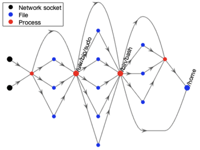
Figure 1: IFG of ransomware attack. Nodes of the graph are color coded to illustrate their respective types (network socket, file, and process). Two network sockets are identified as the entry points of the ransomware attack. Destinations of the attack ($/usr/bin/sudo,/bin/bash,/home$) are labeled in the graph.

Simulations use the following cost, reward, and penalty parameters. Cost parameters: for all $s^{j}_{i}\in{\bf S}$ such that $u_{i}\notin\pazocal{D}_{j}$, $\pazocal{C}_{D}(s_{i}^{j})=-1$ for $j=1$, $\pazocal{C}_{D}(s_{i}^{j})=-2$ for $j=2$, and $\pazocal{C}_{D}(s_{i}^{j})=-3$ for $j=3$. For all other states, $s\in{\bf S}$, $\pazocal{C}_{D}(s)=0$. Rewards: $\alpha_{{\scriptscriptstyle{D}}}^{1}=40$, $\alpha_{{\scriptscriptstyle{D}}}^{2}=80$, $\alpha_{{\scriptscriptstyle{D}}}^{3}=120$, $\beta_{{\scriptscriptstyle{A}}}^{1}=20$, $\beta_{{\scriptscriptstyle{A}}}^{2}=40$, $\beta_{{\scriptscriptstyle{A}}}^{3}=60$, $\sigma_{{\scriptscriptstyle{D}}}^{1}=30$, $\sigma_{{\scriptscriptstyle{D}}}^{2}=50$, and $\sigma_{{\scriptscriptstyle{D}}}^{3}=70$. Penalties: $\alpha_{{\scriptscriptstyle{A}}}^{1}=-20$, $\alpha_{{\scriptscriptstyle{A}}}^{2}=-40$, $\alpha_{{\scriptscriptstyle{A}}}^{3}=-60$, $\beta_{{\scriptscriptstyle{D}}}^{1}=-30$, $\beta_{{\scriptscriptstyle{D}}}^{2}=-60$, $\beta_{{\scriptscriptstyle{D}}}^{3}=-90$, $\sigma_{{\scriptscriptstyle{A}}}^{1}=-30$, $\sigma_{{\scriptscriptstyle{A}}}^{2}=-50$, and $\sigma_{{\scriptscriptstyle{A}}}^{3}=-70$. Learning rates used in the simulations are: $\delta_{v}^{n}=\delta_{\epsilon}^{n}=0.5$ if $n<7000$ and $\delta_{v}^{n}=\delta_{\epsilon}^{n}=\frac{1.6}{\kappa(s,n)}$, otherwise. $\delta_{\rho}=\delta_{\pi}^{n}=1$, if $n<7000$ and $\delta_{\rho}=\frac{1}{1+\tau(n)\log(\tau(n))}$, $\delta_{\pi}^{n}=\frac{1}{\tau(n)}$, otherwise.

Note that the learning rates remain constant until iteration $7000$ and then start decaying. We observed that setting learning rates in this fashion helps the finite time convergence of the algorithm. Here, the term $\kappa(s,n)$ in $\delta_{v}^{n}$ and $\delta_{\epsilon}^{n}$ denotes the total number of times a state $s\in{\bf S}$ is visited from $7000^{\text{th}}$ iteration onwards in Algorithm VI.1. Hence, in our simulations, the learning rates $\delta_{v}^{n}$ of $v^{n}_{k}(s)$ iterates and $\delta_{\epsilon}^{n}$ of the $\epsilon_{k}^{n+1}(s,a_{k})$ iterates depend on the iteration $n$ and the state visited at iteration $n$. The term $\tau(n)=n-6999$.

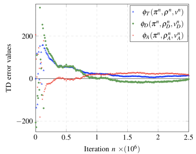
Figure 2: Plots of total Temporal Difference error (TD error), $\phi_{T}(\pi^{n},\rho^{n},v^{n})$, DIFT’s TD error $\phi_{D}(\pi^{n},\rho_{D}^{n},v_{D}^{n})$, and APT’s TD error $\phi_{A}(\pi^{n},\rho_{A}^{n},v_{A}^{n})$ evaluated at iterations $n=1,500,1000,\ldots,2.5\times 10^{6}$ of Algorithm VI.1 for ransomware attack. Values of TD errors at the $n^{\text{th}}$ iteration depend on the policies $\pi^{n}$, average rewards $\rho^{n}$, and value functions $v^{n}$ of DIFT and APT at the $n^{\text{th}}$ iteration. $\phi_{D}(\pi^{n},\rho_{D}^{n},v_{D}^{n})$ and $\phi_{A}(\pi^{n},\rho_{A}^{n},v_{A}^{n})$ are defined in Eqn. (32) and $\phi_{T}(\pi^{n},\rho^{n},v^{n})=\phi_{D}(\pi^{n},\rho_{D}^{n},v_{D}^{n})+\phi_{A}(\pi^{n},\rho_{A}^{n},v_{A}^{n})$.

Conditions (11a) and (11b) in Corollary V.4 are used to validate the convergence of Algorithm VI.1 to an ARNE of the DIFT-APT game. Let $\phi_{T}(\pi,\rho,v)=\phi_{D}(\pi,\rho_{D},v_{D})+\phi_{A}(\pi,\rho_{A},v_{A})$, where $\pi=(\pi_{D},\pi_{A})$, $\rho=(\rho_{D},\rho_{A})$, $v=(v_{D},v_{A})$. Here, $\phi_{k}(\pi,\rho_{k},v_{k})$, for $k\in\{D,A\}$, is given by

$$\begin{split}\phi_{k}(\pi,\rho_{k},v_{k})=&\sum\limits_{s\in{\bf S}}\sum\limits_{a_{k}\in\pazocal{A}_{k}(s)}\Big{(}\rho_{k}+v_{k}(s)-r_{k}(s,a_{k},\pi_{-k})\\ &-\sum\limits_{s^{\prime}\in{\bf S}}\mathbf{P}(s^{\prime}|s,a_{k},\pi_{-k})v_{k}(s^{\prime})\Big{)}\pi_{k}(s,a_{k})=0\end{split}$$ (32)

We refer to $\phi_{T}(\pi,\rho,v)$, $\phi_{D}(\pi,\rho_{D},v_{D})$, and $\phi_{A}(\pi,\rho_{A},v_{A})$ as the total Temporal Difference error (TD error) , DIFT’s TD error, and APT’s TD error, respectively. Then conditions (11a) and (11b) in Corollary V.4 together imply that a policy pair forms an ARNE if and only if $\phi_{D}(\pi,\rho_{D},v_{D})=\phi_{A}(\pi,\rho_{A},v_{A})=0$. Consequently, at ARNE $\phi_{T}(\pi,\rho,v)=0$. Figure 2 plots $\phi_{T}$, $\phi_{D}$, and $\phi_{A}$ corresponding to the policies given by Algorithm VI.1 at iterations $n=1,500,\ldots,2.5\times 10^{6}$. The plots show that $\phi_{T}$, $\phi_{D}$ and $\phi_{A}$ converge very close to $0$ as $n$ increases.

Figure 3 plots the average reward values of DIFT and APT in Algorithm VI.1 at $n=1,500,\ldots,2.5\times 10^{6}$. Figure 3 shows that $\rho_{D}^{n}$ and $\rho_{A}^{n}$ converge as the iteration count $n$ increases.

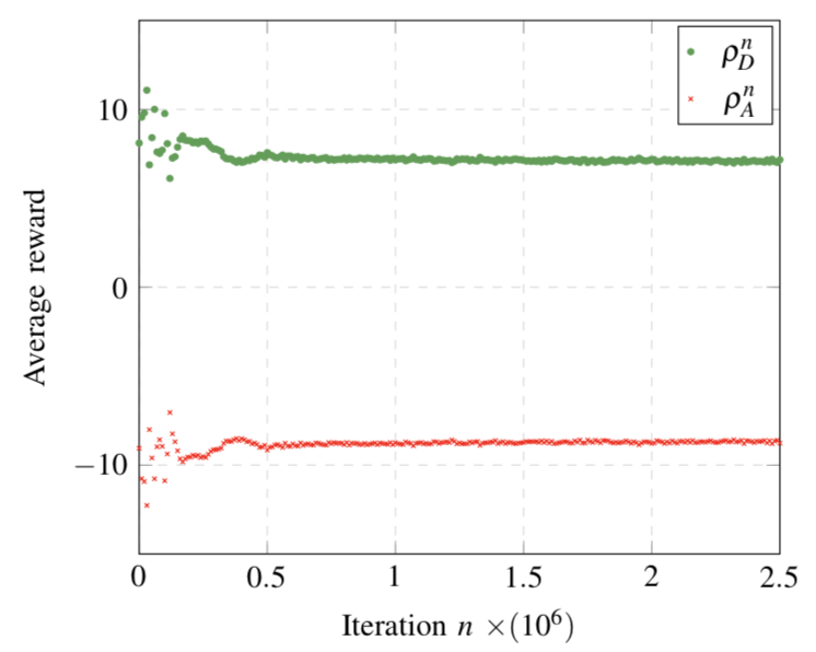
Figure 3: Plots of the average rewards of DIFT $(\rho_{D}^{n})$ and APT $(\rho_{A}^{n})$ at a iteration $n\in\{1,500,1000,\ldots 2.5\times 10^{6}\}$ of Algorithm VI.1. Average rewards at the $n^{\text{th}}$ iteration depend on the policies $(\pi^{n})$ of DIFT and APT.

Figure 4: Comparison of the average rewards of DIFT and APT obtained by the converged policies in Algorithm VI.1 (ARNE policy) against the average rewards of the players obtained by two other policies of DIFT: uniform policy and cut policy. Uniform policy: DIFT chooses an action at every state under a uniform distribution. Cut policy: DIFT performs security analysis at a destination related state, $s^{j}_{i}:u_{i}\in\pazocal{D}_{j}$, with probability one whenever the state of the game is an in-neighbor of that destination related state.

Figure 4 compares the average rewards of the players corresponding to the converged policies in Algorithm VI.1 (ARNE policy) against the average reward values of the players corresponding to two other policies of DIFT, i) uniform policy and ii) cut policy. Note that, in i) DIFT chooses an action at every state under a uniform distribution. Where as in ii) DIFT performs security analysis at a destination related state, $s^{j}_{i}:u_{i}\in\pazocal{D}_{j}$, with probability one whenever the state of the game is an in-neighbor of that destination related state. APT’s policy in both uniform policy and cut policy cases are maintained to be as same as in the case of ARNE policy case. The results show that DIFT achieves a higher average reward under ARNE policy when compared to the uniform and cut policies. Further, results also suggest that APT gets a lower reward under the DIFT’s ARNE policy when compared to the uniform and cut policies.

VIII Conclusion

In this paper we studied the problem of resource efficient and effective detection of Advanced Persistent Threats (APTs) using Dynamic Information Flow Tracking (DIFT) detection mechanism. We modeled the strategic interactions between DIFT and APT as a nonzero-sum, average reward stochastic game. Our game model captures the security costs, false-positives, and false-negatives associated with DIFT to enable resource efficient and effective defense policies. Our model also incorporates the information asymmetry between DIFT and APT that arises from DIFT’s inability to distinguish malicious flows from benign flows and APT’s inability to know the locations where DIFT performs a security analysis. Additionally, the game has incomplete information as the transition probabilities (false-positive and false-negative rates) are unknown. We proposed RL-ARNE to learn an Average Reward Nash Equilibrium (ARNE) of the DIFT-APT game. The proposed algorithm is a multiple-time scale stochastic approximation algorithm. We prove the convergence of RL-ARNE algorithm to an ARNE of the DIFT-APT game.

We evaluated our game model and algorithm on a real-world ransomware attack dataset collected using RAIN framework. Our simulation results showed convergence of the proposed algorithm on the ransomware attack dataset. Further the results showed and validated the effectiveness of the proposed game theoretic framework for devising optimal defense policies to detect APTs. As future work we plan to investigate and model APT attacks by multiple attackers with different capabilities.

Appendix

Lemma VIII.1.

Consider $\Omega_{k,\pi_{-k}}^{s,a_{k}}$ and $\Delta(\pi)$ given in Eqns. (13) and (14), respectively. Then, $\frac{\partial\Delta(\pi)}{\partial\pi_{k}(s,a_{k})}=\sum\limits_{\bar{k}\in\{D,A\}}\Omega_{\bar{k},\pi_{-k}}^{s,a_{k}}$.

Proof.

Recall $k\in\{D,A\}$ and $-k=\{D,A\}\setminus k$.

$$\Delta(\pi)=\sum\limits_{s\in{\bf S}}\left[\sum\limits_{a_{k}\in\pazocal{A}_{k}(s)}\Omega_{k,\pi_{-k}}^{s,a_{k}}\pi_{k}(s,a_{k})+\sum\limits_{a_{-k}\in\pazocal{A}_{-k}(s)}\Omega_{-k,\pi_{k}}^{s,a_{-k}}\pi_{-k}(s,a_{-k})\right].$$

Taking derivative with respect to $\pi_{k}(s,a_{k})$ in Eqn. (14) gives,

$$\frac{\partial\Delta(\pi)}{\partial\pi_{k}(s,a_{k})}=\Omega_{k,\pi_{-k}}^{s,a_{k}}+\sum\limits_{a_{-k}\in\pazocal{A}_{-k}(s)}\frac{\partial\Omega_{-k,\pi_{k}}^{s,a_{-k}}}{\partial\pi_{k}(s,a_{k})}\pi_{-k}(s,a_{-k})$$

From Eqn. (13),

$$\frac{\partial\Omega_{-k,\pi_{k}}^{s,a_{-k}}}{\partial\pi_{k}(s,a_{k})}=\rho_{-k}+v_{-k}(s)-r_{-k}(s,a_{k},a_{-k})-\sum\limits_{s^{\prime}\in{\bf S}}\mathbf{P}(s^{\prime}|s,a_{k},a_{-k})v_{-k}(s^{\prime})$$

Note that,

$$\sum\limits_{a_{-k}\in\pazocal{A}_{-k}(s)}\frac{\partial\Omega_{-k,\pi_{k}}^{s,a_{-k}}}{\partial\pi_{k}(s,a_{k})}\pi_{-k}(s,a_{-k})=\sum\limits_{a_{-k}\in\pazocal{A}_{-k}(s)}\big{[}\rho_{k}+v_{k}(s)-$$

$$r_{k}(s,a_{k},a_{-k})-\sum\limits_{s^{\prime}\in{\bf S}}\mathbf{P}(s^{\prime}|s,a_{k},a_{-k})v_{k}(s^{\prime})\big{]}\pi_{-k}(s,a_{-k})=\Omega_{-k,\pi_{-k}}^{s,a_{k}}$$

Therefore, $\frac{\partial\Delta(\pi)}{\partial\pi_{k}(s,a_{k})}=\sum\limits_{\bar{k}\in\{D,A\}}\Omega_{\bar{k},\pi_{-k}}^{s,a_{k}}.$ This proves the result. ∎

References

- [1] J. Jang-Jaccard and S. Nepal, “A survey of emerging threats in cybersecurity,” Journal of Computer and System Sciences, vol. 80, no. 5, pp. 973–993, 2014.
- [2] B. Watkins, “The impact of cyber attacks on the private sector,” Briefing Paper, Association for International Affair, vol. 12, pp. 1–11, 2014.
- [3] M. Ussath, D. Jaeger, F. Cheng, and C. Meinel, “Advanced persistent threats: Behind the scenes,” Annual Conference on Information Science and Systems (CISS), pp. 181–186, 2016.
- [4] N. Falliere, L. O. Murchu, and E. Chien, “W32. stuxnet dossier,” White paper, Symantec Corp., Security Response, vol. 5, no. 6, pp. 1–69, 2011.
- [5] B. Bencsáth, G. Pék, L. Buttyán, and M. Felegyhazi, “The cousins of Stuxnet: Duqu, Flame, and Gauss,” Future Internet, vol. 4, no. 4, pp. 971–1003, 2012.
- [6] T. Yadav and A. M. Rao, “Technical aspects of cyber kill chain,” International Symposium on Security in Computing and Communication, pp. 438–452, 2015.
- [7] J. Newsome and D. Song, “Dynamic taint analysis: Automatic detection, analysis, and signature generation of exploit attacks on commodity software,” Network and Distributed Systems Security Symposium, 2005.
- [8] J. Clause, W. Li, and A. Orso, “Dytan: A generic dynamic taint analysis framework,” International Symposium on Software Testing and Analysis, pp. 196–206, 2007.
- [9] G. E. Suh, J. W. Lee, D. Zhang, and S. Devadas, “Secure program execution via dynamic information flow tracking,” ACM Sigplan Notices, vol. 39, no. 11, pp. 85–96, 2004.
- [10] G. Brogi and V. V. T. Tong, “TerminAPTor: Highlighting advanced persistent threats through information flow tracking,” IFIP International Conference on New Technologies, Mobility and Security, pp. 1–5, 2016.
- [11] W. Enck, P. Gilbert, S. Han, V. Tendulkar, B.-G. Chun, L. P. Cox, J. Jung, P. McDaniel, and A. N. Sheth, “Taintdroid: An information-flow tracking system for realtime privacy monitoring on smartphones,” ACM Transactions on Computer Systems, vol. 32, no. 2, pp. 1–5, 2014.
- [12] D. Wagner and P. Soto, “Mimicry attacks on host-based intrusion detection systems,” Proceedings of the 9th ACM Conference on Computer and Communications Security, pp. 255–264, 2002.
- [13] Y. Ji, S. Lee, E. Downing, W. Wang, M. Fazzini, T. Kim, A. Orso, and W. Lee, “RAIN: Refinable attack investigation with on-demand inter-process information flow tracking,” ACM SIGSAC Conference on Computer and Communications Security, pp. 377–390, 2017.
- [14] K. Jee, V. P. Kemerlis, A. D. Keromytis, and G. Portokalidis, “Shadowreplica: Efficient parallelization of dynamic data flow tracking,” ACM SIGSAC Conference on Computer & Communications Security, pp. 235–246, 2013.
- [15] E. B. Nightingale, D. Peek, P. M. Chen, and J. Flinn, “Parallelizing security checks on commodity hardware,” ACM Sigplan Notices, vol. 43, no. 3, pp. 308–318, 2008.
- [16] L. S. Shapley, “Stochastic games,” Proceedings of the national academy of sciences, vol. 39, no. 10, pp. 1095–1100, 1953.
- [17] R. Amir, “Stochastic games in economics and related fields: An overview,” Stochastic Games and Applications, pp. 455–470, 2003.
- [18] D. Foster and P. Young, “Stochastic evolutionary game dynamics,” Theoretical Population Biology, vol. 38, no. 2, p. 219, 1990.
- [19] Q. Zhu and T. Başar, “Robust and resilient control design for cyber-physical systems with an application to power systems,” IEEE Decision and Control and European Control Conference (CDC-ECC), pp. 4066–4071, 2011.
- [20] K.-w. Lye and J. M. Wing, “Game strategies in network security,” International Journal of Information Security, vol. 4, no. 1-2, pp. 71–86, 2005.
- [21] J. F. Nash, “Equilibrium points in n-person games,” Proceedings of the national academy of sciences, vol. 36, no. 1, pp. 48–49, 1950.
- [22] J. Filar and K. Vrieze, Competitive Markov Decision Processes. Springer Science & Business Media, 2012.
- [23] M. Sobel, “Noncooperative stochastic games,” The Annals of Mathematical Statistics, vol. 42, no. 6, pp. 1930–1935, 1971.
- [24] J.-F. Mertens and T. Parthasarathy, “Equilibria for discounted stochastic games,” Stochastic Games and Applications, pp. 131–172, 2003.
- [25] T. Raghavan and J. A. Filar, “Algorithms for stochastic games—A survey,” Zeitschrift für Operations Research, vol. 35, no. 6, pp. 437–472, 1991.
- [26] M. Bowling and M. Veloso, “Rational and convergent learning in stochastic games,” International Joint Conference on Artificial Intelligence, vol. 17, no. 1, pp. 1021–1026, 2001.
- [27] J. Hu and M. P. Wellman, “Nash Q-learning for general-sum stochastic games,” Journal of Machine Learning Research, vol. 4, pp. 1039–1069, 2003.
- [28] J. Li, “Learning average reward irreducible stochastic games: Analysis and applications,” Ph.D. dissertation, Dept. Ind. Manage. Syst. Eng., Univ. South Florida, Tampa, FL, USA, 2003.
- [29] H. L. Prasad, L. A. Prashanth, and S. Bhatnagar, “Two-timescale algorithms for learning Nash equilibria in general-sum stochastic games,” International Conference on Autonomous Agents and Multiagent Systems, pp. 1371–1379, 2015.
- [30] T. Alpcan and T. Başar, Network security: A decision and game-theoretic approach. Cambridge University Press, 2010.
- [31] T. Alpcan and T. Başar, “An intrusion detection game with limited observations,” International Symposium on Dynamic Games and Applications, 2006.
- [32] K. C. Nguyen, T. Alpcan, and T. Başar, “Stochastic games for security in networks with interdependent nodes,” International Conference on Game Theory for Networks, pp. 697–703, 2009.
- [33] M. Panfili, A. Giuseppi, A. Fiaschetti, H. B. Al-Jibreen, A. Pietrabissa, and F. D. Priscoli, “A game-theoretical approach to cyber-security of critical infrastructures based on multi-agent reinforcement learning,” in 2018 26th Mediterranean Conference on Control and Automation (MED). IEEE, 2018, pp. 460–465.
- [34] R. Klima, K. Tuyls, and F. Oliehoek, “Markov security games: Learning in spatial security problems,” in NIPS Workshop on Learning, Inference and Control of Multi-Agent Systems, 2016, pp. 1–8.
- [35] L. Huang and Q. Zhu, “Adaptive strategic cyber defense for advanced persistent threats in critical infrastructure networks,” ACM SIGMETRICS Performance Evaluation Review, vol. 46, no. 2, pp. 52–56, 2019.
- [36] M. O. Sayin, H. Hosseini, R. Poovendran, and T. Başar, “A game theoretical framework for inter-process adversarial intervention detection,” International Conference on Decision and Game Theory for Security, pp. 486–507, 2018.
- [37] S. Moothedath, D. Sahabandu, J. Allen, A. Clark, L. Bushnell, W. Lee, and R. Poovendran, “A game-theoretic approach for dynamic information flow tracking to detect multi-stage advanced persistent threats,” IEEE Transactions on Automatic Control, 2020.
- [38] S. Moothedath, D. Sahabandu, A. Clark, S. Lee, W. Lee, and R. Poovendran, “Multi-stage dynamic information flow tracking game,” Conference on Decision and Game Theory for Security, Lecture Notes in Computer Science, vol. 11199, pp. 80–101, 2018.
- [39] D. Sahabandu, B. Xiao, A. Clark, S. Lee, W. Lee, and R. Poovendran, “DIFT games: Dynamic information flow tracking games for advanced persistent threats,” IEEE Conference on Decision and Control (CDC), pp. 1136–1143, 2018.
- [40] D. Sahabandu, S. Moothedath, J. Allen, A. Clark, L. Bushnell, W. Lee, and R. Poovendran, “A game theoretic approach for dynamic information flow tracking with conditional branching,” American Control Conference (ACC), pp. 2289–2296, 2019.
- [41] S. Moothedath, D. Sahabandu, J. Allen, A. Clark, L. Bushnell, W. Lee, and R. Poovendran, “Dynamic Information Flow Tracking for Detection of Advanced Persistent Threats: A Stochastic Game Approach,” ArXiv e-prints, p. arXiv:2006.12327, 2020.
- [42] S. Misra, S. Moothedath, H. Hosseini, J. Allen, L. Bushnell, W. Lee, and R. Poovendran, “Learning equilibria in stochastic information flow tracking games with partial knowledge,” IEEE Conference on Decision and Control (CDC), pp. 4053–4060, 2019.
- [43] D. Sahabandu, S. Moothedath, J. Allen, L. Bushnell, W. Lee, and R. Poovendran, “Stochastic dynamic information flow tracking game with reinforcement learning,” International Conference on Decision and Game Theory for Security, pp. 417–438, 2019.
- [44] V. S. Borkar, “Stochastic approximation with two time scales,” Systems & Control Letters, vol. 29, no. 5, pp. 291–294, 1997.
- [45] S. M. Milajerdi, R. Gjomemo, B. Eshete, R. Sekar, and V. Venkatakrishnan, “Holmes: real-time APT detection through correlation of suspicious information flows,” IEEE Symposium on Security and Privacy (SP), pp. 1137–1152, 2019.
- [46] V. S. Borkar, Stochastic approximation: a dynamical systems viewpoint. Springer, 2009, vol. 48.
- [47] D. P. Bertsekas and J. N. Tsitsiklis, Neuro-Dynamic Programming. Athena Scientific, 1996.
- [48] J. N. Tsitsiklis, “Asynchronous stochastic approximation and Q-Learning,” Machine learning, vol. 16, no. 3, pp. 185–202, 1994.
- [49] K. Soumyanath and V. S. Borkar, “An analog scheme for fixed-point computation-part ii: Applications,” IEEE Transactions on Circuits and Systems I: Fundamental Theory and Applications, vol. 46, no. 4, pp. 442–451, 1999.
- [50] M. Metivier and P. Priouret, “Applications of a kushner and clark lemma to general classes of stochastic algorithms,” IEEE Transactions on Information Theory, vol. 30, no. 2, pp. 140–151, 1984.
- [51] S. Bhatnagar, R. S. Sutton, M. Ghavamzadeh, and M. Lee, “Natural actor–critic algorithms,” Automatica, vol. 45, no. 11, pp. 2471–2482, 2009.