Boosting the efficiency of ab initio electron-phonon coupling calculations through dual interpolation

Abstract

The coupling between electrons and phonons in solids plays a central role in describing many phenomena, including superconductivity and thermoelecric transport. Calculations of this coupling are exceedingly demanding as they necessitate integrations over both the electron and phonon momenta, both of which span the Brillouin zone of the crystal, independently. We present here an ab initio method for efficiently calculating electron-phonon mediated transport properties by dramatically accelerating the computation of the double integrals with a dual interpolation technique that combines maximally localized Wannier functions with symmetry-adapted plane waves. The performance gain in relation to the current state-of-the-art Wannier-Fourier interpolation is approximately $2n_{s}\times M$, where $n_{s}$ is the number of crystal symmetry operations and $M$, a number in the range $5-60$, governs the expansion in star functions. We demonstrate with several examples how our method performs some ab initio calculations involving electron-phonon interactions.

The electron-boson coupling is ubiquitous in physical phenomena through the whole spectrum of the physics of solids. In particular, electron-phonon (el-ph) coupling plays a fundamental role in the renormalization of electronic and vibrational energy scales, thus determining the coupling itself, with important consequences for transport propertiesGiustino (2017); Marini (2008); Park et al. (2007); Restrepo et al. (2009). Conventional superconductivity is a case in point, where the interactions between electrons and phonons give rise to Cooper pairing.Margine and Giustino (2014) Other examples include the temperature dependence of electronic conductivity and thermoelectric transport properties,Fiorentini and Bonini (2016); Wang et al. (2011) as well as phonon-assisted optical absorption in indirect-gap semiconductors.Noffsinger et al. (2012) Interest in thermoelectrics has increased rapidly in recent years, partly due to the expectation of discovering higher figure-of-merit materials, boosted by the nanotechnology revolution. Boukai et al. (2011) A major goal of theory has been to predict thermoelectric transport properties directly from atomistic-scale calculations without any adjustable or empirical parameters,Restrepo et al. (2009); Wang et al. (2011); Fiorentini and Bonini (2016) particularly combining density functional theory (DFT) and many-body perturbation theory. Despite great advances, such calculations remain very demanding and still pose a challenge, even for simple crystalline bulk systems.

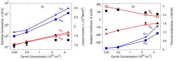
Figure 1: Thermoelectric transport properties ${\it{TP}}$ for p- and n-type doped Si polycrystals: (a) Electrical conductivity, $\sigma$, (red) compared with experimental valuesStrasser et al. (2004) (filled black symbols) and Lorenz function, $\Lambda$, (blue); (b) Seebeck coefficient, S, (red) compared with experimental dataStrasser et al. (2004) (filled black symbols) and thermal conductivity due to the carriers, $\kappa$, (blue) calculated from the relaxation times due to scatterings by el-ph coupling and ionized impurities (see text for details).

A well-established approach, using a first-principles description of el-ph coupling, relies on solving the el-ph matrix elements through density-functional perturbation theory (DFPT)Baroni et al. (2001). The el-ph matrix elements, $g({\bf{k}},{\bf{k+q}})=(\bra{{\bf{k}}+{\bf{q}}}{\delta}_{{\bf{q}},\beta}V^{KS}\ket{{\bf{k}}})_{uc}$, correspond to the electronic scattering calculated from the variations of the Kohn-Sham (KS) potential due to phonon perturbations with wavevector $\bf{q}$ and branch index $\beta$ within the unit cell ($uc$). To obtain transport properties (TP), $|g(\bf{k},\bf{k+q})|^{2}$ must be integrated over the electron and phonon momenta, both spanning the entire Brillouin Zone (BZ), independently. This double integration requires very fine sampling of the electron and phonon wavevectors to achieve numerical convergence, which represents the bulk of the computational burden. The application of crystal symmetry properties for the full integration of TP, which depend directly on the el-ph matrix elements, is not allowed. Even if the wavevector ${\bf{k}}$ in the el-ph matrix element lies within the symmetry-reduced portion (irreducible wedge) of the BZ, the transferred momenta ${\bf{k+q}}$ spread out in the whole zone because ${\bf{q}}$ belongs to an uniform mesh. Dense sampling of the BZ is prohibitive, the reason being the connection between transferred momenta with equally dense ${\bf{k}}$-point meshes.

Specialized numerical techniques have been developed to address this problem. One attempt to simplify the brute-force integration is based on pre-screening of subsets of the reciprocal space, such as relevant conduction pockets within the neighborhood of band extrema that significantly contribute to the integral. Alternatively, interpolation schemes, such as linearLi (2015) or Wannier-basedGiustino et al. (2007); Giustino (2017) ones, have been developed to improve convergence. In particular, the interpolation of the el-ph matrix elements on the basis of Wannier functions introduced by Giustino, Cohen, and Louie,Giustino et al. (2007) has proven very successful in calculating properties with more favorable scaling than using directly the DFPT approach. In this Letter, we present a novel method for the computation of el-ph mediated TP which uses two interpolations: the first one is the usual Wannier-Fourier (W-F) interpolation, followed by a second one based on symmetry-adapted plane-waves (PW). Our method leads to an efficient sampling of extremely fine, homogeneous ${\bf{k}}$ and ${\bf{q}}$ grids, with a significant decrease in computational cost compared to W-F calculations with a single interpolation.

To illustrate the capability of our method, we considered realistic properties of solids (see SM for more details). Fig. 1 shows the calculated thermoelectric $\it{TP}$ for Si polycrystals using our dual interpolation method to calculate the relaxation time within the Boltzmann transport equation (BTE). We calculated the electrical conductivity, $\sigma$, Seebeck coefficient, S, Lorenz function, $\Lambda$, and thermal conductivity due to the carriers, $\kappa$, as functions of carrier concentration. Our results for $n$ and $p$-doped Si polycrystals agree reasonably well with available experimental $\it{TP}$. For these calculations we also included the scattering by ionized impurities, within the Brooks-Herring theory (see SM), considering in all calculations a fixed unitary ratio between impurities and carrier concentrations, which are the only input parameter along with the crystal structure. Fig. 2 shows the results of phonon-assisted optical absorption for Si at $296$K and $78$K as a function of the photon energies. Our calculations, based on our dual interpolation method and the theory developed by Hall, Bardeen and Blatt (see Noffsinger et al. (2012)), are in good agreement with experimental results.

Before presenting our method we review the basic concept and analyze the advantages and drawbacks of W-F interpolation. Using W-F interpolation, the el-ph matrix elements $g(\mathbf{k},\mathbf{q})$ can be calculated on coarse $\mathbf{k},\mathbf{q}$ meshes and then interpolated onto much finer $\mathbf{k}^{\prime},\mathbf{q}^{\prime}$ meshes through simple matrix multiplication.Giustino et al. (2007) The matrix elements on the fine mesh are given by

$$g({\bf{k^{\prime}}},{\bf{q^{\prime}}})=\frac{1}{N_{e}}\sum_{{\bf{R}}_{e},{\bf{R}}_{p}}e^{i({\bf{k^{\prime}}}\cdot{\bf{R}}_{e}+{\bf{q^{\prime}}}\cdot{\bf{R}}_{p})}{\bf{U}}_{{\bf{k^{\prime}}}+{\bf{q^{\prime}}}}g({\bf{R}}_{e},{\bf{R}}_{p}){\bf{U}}_{{\bf{k^{\prime}}}}^{\dagger}{\bf{u}}_{\bf{q^{\prime}}},$$ (1)

where ${\bf{R}}_{e}$ and ${\bf{R}}_{p}$ are primitive lattice vectors of the Wigner-Seitz (WS) supercell with Born-von-Kármán (BvK) periodic boundary conditions, U${}_{{\bf{k^{\prime}}}}$ (u${}_{{\bf{q^{\prime}}}}$) is a diagonalizer matrix over ${\bf{k^{\prime}}}$ (${\bf{q^{\prime}}}$) indices from Wannier to Bloch representations for electrons (phonons) and the el-ph matrix elements in the Wannier representation are given by

$$g({\bf{R}}_{e},{\bf{R}}_{p})=\frac{1}{N_{p}}\sum_{{\bf{k}},{\bf{q}}}e^{-i({\bf{k}}\cdot{\bf{R}}_{e}+{\bf{q}}\cdot{\bf{R}}_{p})}{\bf{U}}_{{\bf{k}}+{\bf{q}}}^{\dagger}g({\bf{k}},{\bf{q}}){\bf{U}}_{{\bf{k}}}{\bf{u}}_{{\bf{q}}}^{-1}\leavevmode\nobreak\ ,$$ (2)

U_k is a unitary matrix corresponding to the rotation of the corresponding electronic states from Bloch to Wannier representations within the gauge of maximally localized Wannier functions (MLWF),Marzari and Vanderbilt (1997) and u_q is a unitary rotation matrix from Bloch to MLWF for phonons. The strength of the W-F interpolation method is the fact that one only needs to perform calculations over the initial coarse $\bf{k},\bf{q}$ meshes, and then can use Eq. (1) to determine $g(\bf{k}^{\prime},\bf{q}^{\prime})$ on finer $\bf{k^{\prime}},\bf{q^{\prime}}$ meshes. For this, we neglect the matrix elements outside the WS supercell generated from the initial coarse BZ mesh.

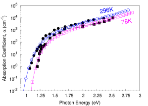
Figure 2: Phonon-assisted optical absorption, $\alpha$, of Si at $296$K and $78$K as a function of photon energies. Our results (blue and magenta) are in good agreement with corresponding experimental results (black)Braunstein et al. (1958).

The accuracy of W-F calculations strongly depends on the spatial localization of $g({\bf{R}}_{e},{\bf{R}}_{p})$ within Eq. (1). A more detailed analysis suggests $g({\bf{R}}_{e},{\bf{R}}_{p})$ should decay in the variable ${\bf{R}}_{e}$ at least with the rapidity of MLWFs. For ${\bf{R}}_{e}=0$, $g(0,{\bf{R}}_{p})$ decays with ${\bf{R}}_{p}$ due to the screened Coulomb interaction of the dipole potential generated by atomic displacement. Thus the localization of $g({\bf{R}}_{e},{\bf{R}}_{p})$ depends strongly on the dielectric properties of the system. In particular, Friedel oscilationsFetter and Walecka (2012) ($|{\bf{R}}_{p}|^{-3}$) and quadrupole behaviorPick et al. (1970) ($|{\bf{R}}_{p}|^{-4}$) are intimately related to the screening properties of metals and nonpolar semiconductors, respectively.

Despite the advantages of the W-F interpolation and its more favorable scaling, there are still some drawbacks. The method is computationally intensive when many $\bf{k}$/$\bf{q}$ points are needed to achieve converged values for TP. The main computational operations are the simple matrix multiplications shown in Eq. 1, with a computational complexity of $\mathcal{O}(n^{3})$ for classical computation, where $n$ is the matrix size involved. For final dense grids with $N_{f}^{{\bf{k^{\prime}}}}$ ($N_{f}^{{\bf{q^{\prime}}}}$) ${\bf{k^{\prime}}}$ (${\bf{q^{\prime}}}$) points, the number of floating-point operations reach $\approx N_{f}^{\bf{k^{\prime}}}\times N_{f}^{\bf{q^{\prime}}}n^{3}$. To reduce the computational cost of Wannier-based calculations, some strategies have been adopted, including double grid schemesFiorentini and Bonini (2016) or (quasi) Monte-Carlo (MC) integrations.Poncé et al. (2014) In the former, only the bandstructure and phonon dispersion are calculated over an ultrafine grid ($N_{f}\times N_{f}\times N_{f}$), while el-ph matrix elements are computed over a moderate grid ($N_{el-ph}\times N_{el-ph}\times N_{el-ph}$, with $N_{el-ph}=s\times N_{f}$ and $s=1/2,1/3$) and extrapolated to the ultrafine grid assuming that the el-ph coupling function is smooth. The drawbacks here consist of the extrapolation which is often fraught with risk, and the very modest gain factor of the method. On the other hand, by using (quasi) MC integration, one has to test very dense sets of random (or quasi-random) $\bf{k}$ or $\bf{q}$-points, which is a serious drawback.

Our method proceeds as follows. For clarity, we describe the procedure for doing the partial $\mathbf{q}^{\prime}$ integration first, but one can easily switch the order of integration. We begin by computing $g(\mathbf{k},\mathbf{q})$ over coarse $\mathbf{k}$ and $\mathbf{q}$ meshes. Next, using W-F interpolation, we determine $g$ over a finer $\mathbf{q}^{\prime}$ mesh and perform the partial integration at each of the $n_{\mathbf{\bar{k}}}$ irreducible $\mathbf{k}$-points, ${\bf{\bar{k}}}_{l}$, corresponding to a moderate regular $\mathbf{k}$-mesh (${\bf{k^{r}}}$). Thus we obtain a function $f({\bf{\bar{k}}}_{l})\propto\int_{BZ}|g({\bf{\bar{k}}}_{l}+{\bf{q^{\prime}}},{\bf{\bar{k}}}_{l})|^{2}d{{\bf{q^{\prime}}}}$ containing first-principles el-ph coupling properties defined at selected high-symmetry points in the corresponding $\mathbf{k}$-space. Given $f(\mathbf{\bar{k}}_{l})$, the next goal is to find a smooth interpolation over the whole $\mathbf{k}$-space on a finer grid. Such an interpolation problem may present severe difficulties if one uses an inadequate basis set. We show below that such an interpolation over the entire BZ, combined with periodic or other boundary conditions, can be properly constructed from a basis set possessing the appropriate crystal symmetry.

As the full symmetry of the crystal’s reciprocal space is contained in the function $f({\bf{\bar{k}}}_{l})$, it is natural to use symmetry-adapted PW or star functions, $\Upsilon_{m}({\bf{k^{\prime}}})$, as a basis set to Fourier expand $f$ Chadi and Cohen (1973):

$$\tilde{f}({\bf{k^{\prime}}})=\sum_{m=1}^{M}a_{m}\Upsilon_{m}({\bf{k^{\prime}}})\leavevmode\nobreak\ ,$$ (3)

where $\Upsilon_{m}({\bf{k^{\prime}}})=\frac{1}{n_{s}}\sum_{\{\upsilon\}}\exp({i(\upsilon{\bf{R}}_{m})\cdot{\bf{k^{\prime}}}})\leavevmode\nobreak\ ,$ with the sum running over all $n_{s}$ point group symmetry operations $\{\upsilon\}$ on the direct lattice translations, ${\bf{R}}_{m}$. Star functions obey orthogonality relations involving BZ summationsChadi and Cohen (1973), are totally symmetric under all point-group operations, and are ordered such that the magnitude of $\bf{R_{m}}$ is nondecreasing as $m$ increases, defining each star function to a given shell of lattice vectors. By taking into account the symmetry, it is expected that this expansion would converge much faster than using a regular Fourier expansion. Following the approach proposed by Shankland-Koelling-WoodShankland (1971); Koelling and Wood (1986), we take the number of star functions in the expansion, $M$, to be greater than the number of data points ($M>n_{{\bf{\bar{k}}}}$). We then require the fit function, $\tilde{f}$, to pass through the data points and use the extra freedom from additional basis functions to minimize a spline-like roughness functional in order to suppress oscillations between data points, resulting in a well behaved function throughout the BZ.

We adopt the spline-like roughness functional defined by Pickett, Krakauer and Allen Pickett et al. (1988),

$$\Pi=\sum_{m=2}^{M}\lvert a_{m}\lvert^{2}\rho(R_{m})$$ (4)

with $\rho(R_{m})=\left(1-c_{1}\left({\frac{R_{m}}{R_{min}}}\right)^{2}\right)^{2}+c_{2}(\frac{R_{m}}{R_{min}})^{6}\leavevmode\nobreak\ ,$ where $R_{m}=\lvert{\bf{R}}_{m}\lvert$, $R_{min}$ is the magnitude of the smallest nonzero lattice vector, and $c_{1}=c_{2}=3/4$. Such a functional is more physically appealing than the original functional proposed by Shankland-Koelling-Wood, in the sense that departures of $\tilde{f}$ is minimized from its mean value, $a_{1}$, instead of zero. The main problem in the expansion by star functions in Eq. (3) is the determination of the Fourier coefficients, $a_{m}$. Thus, a Lagrange multiplier method can be used toward this goal, once the problem has been reduced to minimizing ${\Pi}$ subject to the constraints, $\tilde{f}({\bf{\bar{k}}}_{l})={f}({\bf{\bar{k}}}_{l})$, in relation to $a_{m}$. Consequently, the result of this minimization is

$$a_{m}=\begin{cases}\rho(R_{m})^{-1}\sum_{l=1}^{n_{\bf{\bar{k}}}-1}\lambda^{*}_{l}\left[\Upsilon_{m}^{*}({\bf{\bar{k}}}_{l})-\Upsilon_{m}^{*}({\bf{\bar{k}}}_{n_{{\bf{\bar{k}}}}})\right],&m>1,\\ f({\bf{\bar{k}}}_{n_{\bf{\bar{k}}}})-\sum_{m=2}^{M}a_{m}\Upsilon_{m}({\bf{\bar{k}}}_{n_{{\bf{\bar{k}}}}}),&m=1,\end{cases}$$ (5)

in which the Lagrange multipliers, $\lambda^{*}_{l}$, can be evaluated from

$$f({\bf{\bar{k}}}_{p})-f({\bf{\bar{k}}}_{n_{{\bf{\bar{k}}}}})=\sum_{l=1}^{n_{{\bf{\bar{k}}}}-1}{\bf{H}}_{pl}\lambda^{*}_{l}\leavevmode\nobreak\ ,$$ (6)

with

$${\bf{H}}_{pl}=\sum_{m=2}^{M}\frac{\left[\Upsilon_{m}({\bf{\bar{k}}}_{p})-\Upsilon_{m}({\bf{\bar{k}}}_{n_{{\bf{\bar{k}}}}})\right]\left[\Upsilon_{m}^{*}({\bf{\bar{k}}}_{l})-\Upsilon_{m}^{*}({\bf{\bar{k}}}_{n_{{\bf{\bar{k}}}}})\right]}{\rho(R_{m})}\leavevmode\nobreak\ ,$$ (7)

a positive-definite symmetric matrix that can be determined once for a given crystal problem and can be easily crafted numerically.

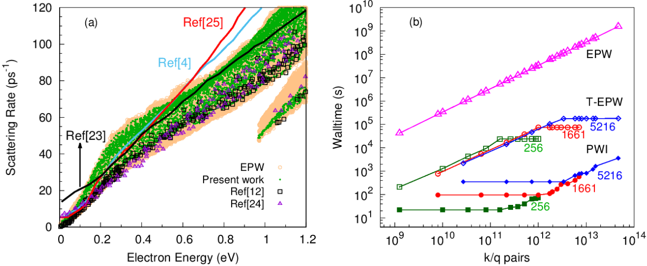
Figure 3: (a) Scattering rates for Si at $300$ K calculated with the dual interpolation method (green dots), DFT with linear interpolation (blackSun et al. (2012) and light blueRestrepo et al. (2009) lines and black squaresLi (2015)), W-F interpolation using EPW (purple trianglesQiu et al. (2015) and light orange circles), and tight-binding calculations (redRideau et al. (2011) line). The W-F calculations used $(30)^{3}$ k/$(60)^{3}$ q ($(100)^{3}$ k/$(40)^{3}$ q) meshes in calculations represented by the purple triangles (orange circles). (b) Walltime required to perform calculations for the electron self-energy due to el-ph coupling in the Fan-Migdal approximation, for different grid sizes. Empty magenta triangles correspond to the direct calculation using EPW over homogeneous grids. Empty (filled) green squares, empty (filled) red circles and empty (filled) blue diamonds correspond to the calculations using T-EPW (only second PW interpolation), starting from $256$, $1661$ and $5216$ irreducible $\mathbf{k}$ points, respectively (see text for details).

Once the Fourier coefficients are determined, a representation of $\tilde{f}$ is generated, which can be written more clearly as a linear mapping of the W-F data,

$$\tilde{f}({\bf{k^{\prime}}})=\sum_{l=1}^{n_{{\bf{\bar{k}}}}-1}J({\bf{\bar{k}}}_{l},{\bf{k^{\prime}}})[f({\bf{\bar{k}}}_{l})-f({\bf{\bar{k}}}_{n_{{\bf{\bar{k}}}}})]\leavevmode\nobreak\ ,$$ (8)

where $J$ is the interpolation formula given by

$$J({\bf{\bar{k}}}_{l},{\bf{k^{\prime}}})=\sum_{p=1}^{n_{{\bf{\bar{k}}}}-1}\sum_{m}^{M}\frac{[\Upsilon_{m}^{*}({\bf{\bar{k}}}_{p})-\Upsilon_{m}^{*}({\bf{\bar{k}}}_{n_{{\bf{\bar{k}}}}})]\Upsilon_{m}({\bf{k^{\prime}}})}{\rho(R_{m}){\bf{H}}_{pl}}\leavevmode\nobreak\ ,$$ (9)

which transforms one ${\bf{k}}$-mesh into another one, that is, ${\bf{\bar{k}}}_{l}\rightarrow{\bf{k^{\prime}}}$. This is the main result of our approach, which allows great computational savings by transforming the W-F data obtained over the ${\bf{k}}$-mesh of irreducible points (${\bf{\bar{k}}}_{l}$) into a homogeneous dense grid (${\bf{k^{\prime}}}$) that is larger than the regular grid (${\bf{k^{r}}}$) that generates such irreducible points. One important point to stress is that $J$ does not depend on data, but it is completely defined by the lattice, namely the set of irreducible sampling (${\bf{\bar{k}}}_{l}$), the number of star functions ($M$), and the form of spline-like roughness functional ($\Pi$). In practice, in order to get a denser mesh, we rely on a Fast Fourier Transform (FFT) from the real space to the reciprocal space in order to compute the expansion given in Eq. (3). We take advantage of the BvK periodic boundary conditions to increase the real space by the expansion factor, $M$, as will be explained below, to get proportionally a new homogeneous ${\bf{k^{\prime}}}$-mesh finer than the original one. As a result we get the full integration over very fine ${\bf{k^{\prime}}}$ and ${\bf{q^{\prime}}}$ meshes in order to calculate transport properties, that is, $TP\propto\sum_{{\bf{k^{\prime}}}}\tilde{f}({\bf{k^{\prime}}})\leavevmode\nobreak\ .$

Our implementation for the second interpolation is based on modifications and adaptations of some subroutines of the BoltzTraPMadsen and Singh (2006) code. Lattice points and their respective star functions are generated in the real space following point group operations of crystal symmetry. The corresponding translation vectors can be given as ${\bf{R}}=u_{1}{\bf{a_{1}}}+u_{2}{\bf{a_{2}}}+u_{3}{\bf{a_{3}}}$, in which ${\bf{a_{1}}}$, ${\bf{a_{2}}}$, ${\bf{a_{3}}}$ are related to the crystal’s direct primitive vectors. Such points are generated inside a sphere with a radius defined as $R^{\prime}=\sqrt[3]{3\cdot n_{{\bf{\bar{k}}}}\cdot n_{s}\cdot M\cdot\Omega/4\pi}$, in which $\Omega$ is the volume of the unit cell. Consequently, $R^{\prime}$ determines the full extension of the real space and can be properly increased, for example, by increasing $M$, the number of star functions per ${\bf{k}}$-point. In order to capture crystal anisotropy, the extension of the real space can be determined for each crystal direction, defining spheres for each crystallographic axis with the maximum radius given by $R_{max}(t)=INT(R^{\prime}\cdot\sqrt{{\bf{b_{t}}}\cdot{\bf{b_{t}}}})+1$, where ${\bf{b_{t}}}$ are the respective reciprocal primitive vectors, with $t=\{1,2,3\}$, and $INT(x)$ takes the largest integer number that does not exceed the magnitude of $x$.

The star functions are ordered in such a way that the magnitude of $\bf{R}_{m}$ is nondecreasing as $m$ increases. Thus, a 3D array containing all vectors are sorted considering their concentric radius, $r$, from the sphere center defined for each axis, and provided that all vectors, ${\bf{R}}$, have different star functions, $m$. The magnitude of each $\bf{R}_{m}$ vector is defined through the metric tensor formalism. For all $\bf{R}_{m}$ in the Bravais lattice, the reciprocal lattice is characterized by a set of wavevectors ${\bf{k}}$, such that, $e^{2\pi i{\bf{k}}\cdot{\bf{R}}_{m}}=1$. Given ${\bf{R}}_{m}$ and ${\bf{k}}$ in the same direction, the magnitude of the vector ${\bf{k}}$ in the reciprocal space is given by $\left|{\bf{k}}\right|=(k_{1}u_{1}+k_{2}u_{2}+k_{3}u_{3})/r=(n_{int}(1)+n_{int}(2)+n_{int}(3))/r$, where $n_{int}(t)=1,2,...,k_{max}(t)$ are integer numbers with $k_{max}(t)=2R_{max}(t)+1$. To determine all $\bf{k}$ vectors from $\bf{R}_{m}$, a 3D FFT is performed. In practice, $k_{max}(t)$ defines the number of data points on each dimension and should be carefully taken as the product of small primes in order to improve the efficiency of FFT.

In fact, the FFT computational complexity is $\mathcal{O}(N\log{}N)$, where $N$ corresponds to the number of data points related to the product of FFT dimensions, namely $N=k_{max}(1)\times k_{max}(2)\times k_{max}(3)\approx 8R^{{\prime}^{3}}\cdot\sqrt{{\bf{b_{1}}}\cdot{\bf{b_{1}}}}\cdot\sqrt{{\bf{b_{2}}}\cdot{\bf{b_{2}}}}\cdot\sqrt{{\bf{b_{3}}}\cdot{\bf{b_{3}}}}\approx 6/\pi({n_{{\bf{\bar{k}}}}}\times n_{s}\times M)$. Consequently, the number of floating-point operations by using our approach is $\approx N_{f}^{{\bf{q^{\prime}}}}\times{n_{{\bf{\bar{k}}}}}n^{3}+6/\pi({n_{{\bf{\bar{k}}}}}\times n_{s}\times M)\ln{(6/\pi({n_{{\bf{\bar{k}}}}}\times n_{s}\times M))}$. The first term comes from the first W-F interpolation by using $n_{{\bf{\bar{k}}}}$ irreducible points, while the second one comes from the symmetry-adapted PW interpolation. The gain in performance by using our method in comparison with single W-F calculation, to get approximately the same final homogeneous grid, can be given by $\approx 2(n_{s}\times M)$, assuming $N_{f}^{\bf{k^{\prime}}}\approx N$ and $N_{f}^{{\bf{k^{\prime}}}}=N_{f}^{{\bf{q^{\prime}}}}$. Clearly, high symmetry systems allow greater computational savings, however the factor $M$, typically ranging from $5-60$ enables remarkably significant performance gain even for low symmetry systems.

In order to test our implementation, we carried out TP calculations for silicon. We computed the imaginary part of the electron self-energy in the Fan-Migdal approximation, $\imaginary\Sigma$, which gives the relaxation time due to e-ph scattering, and consequently, thermoelectric TP using the BTE, as shown in Fig. 1. Additionally, we also studied phonon-assisted optical absorption for Si, as shown in Fig. 2. More details about these calculations can be found in the Supplemental Material (SM). Since the first step in computing the double BZ integrals is based on a W-F interpolation, our implementation has been built on top of the Electron-Phonon Wannier (EPW) Poncé et al. (2016) code, which is contained in the Quantum Espresso package Giannozzi et al. (2009). We have modified the EPW code in order to include the second PW interpolation, as described above, which we call Turbo-EPW (T-EPW). In Fig. 3(a) we show $\imaginary\Sigma$ for Si at 300 K calculated using T-EPW in comparison with other approaches, namely, previous DFT with linear interpolationSun et al. (2012); Restrepo et al. (2009); Li (2015), W-F interpolation with EPWQiu et al. (2015), and tight-binding calculationsRideau et al. (2011). Our results, calculated using $(100)^{3}{\bf{k^{\prime}}}$/$(100)^{3}{\bf{q^{\prime}}}$ grids, are in good agreement with other W-F calculations using the EPW code directly on $(30)^{3}{\bf{k^{\prime}}}/(60)^{3}{\bf{q^{\prime}}}$Qiu et al. (2015) and $(100)^{3}{\bf{k^{\prime}}}/(40)^{3}{\bf{q^{\prime}}}$ grids, but with significantly reduced computational time.

In order to estimate the performance gain of our approach, in Fig. 3(b) we show the computational time required to finalize the calculation of $\imaginary\Sigma$ for different ${\bf{k^{\prime}}}$/${\bf{q^{\prime}}}$ grids, all using the same computational hardware. The time required for calculations based only on W-F interpolations (EPW) grows almost exponentially with increasing ${\bf{k^{\prime}}}$/${\bf{q^{\prime}}}$ density. By applying our method a drastic reduction in the computational time is obtained, which is generally greater than two orders of magnitude, as can be observed from the curves for the total time of T-EPW. These curves also demonstrate a roughly exponential growth with ${\bf{k^{\prime}}}$/${\bf{q^{\prime}}}$ density, which is due to increasing the grid size in the first W-F interpolation, independent of the number of initial irreducible points ${\bf{\bar{k}}}_{l}$. In these test calculations we considered $n_{{\bf{\bar{k}}}}=256,1661,5216$, leading to regular meshes of ${\bf{{k^{r}}}}=(20)^{3},(40)^{3},(50)^{3}$. The plateaus in the computational time for T-EPW are due to increasing the value of $M$ from $5$ to $60$, while keeping fixed the grid of first W-F interpolation ($(100)^{3}{\bf{q^{\prime}}}$ points). As shown in Fig. 3(b), using PW interpolation one can achieve much denser grids by increasing the value of $M$ with negligible increase in computational time. As shown in the SM, the accompanying error due to the increase of $M$ to generate denser grids diminishes by increasing $n_{{\bf{{\bar{k}}}}}$; a solution that can also be used to minimize errors from possible kink structures derived from band crossings, which leads to a Gibbs ringing in Fourier series analysis.

In summary, our method can be used to calculate efficiently el-ph-based ${\it{TP}}$. The computational performance gain is remarkable, being $\approx 2(n_{s}\times M)$ faster than state-of-the-art EPW calculations without loosing accuracy. It should be emphasized that this novel approach can also be used as an efficient and stable numerical tool in order to calculate ubiquitous double BZ integrals, and potentially extending to many further applications, for instance phonon-assisted nonlinear optical properties, superconducting critical temperature and its related thermodynamic properties and electron-plasmon coupling ${\it{TP}}$ from first-principles. Moreover, this method may allow previously impractical calculations and can serve as a starting point to explore the effects of the vertex corrections to the Migdal approximation as well as to address the e-ph coupling in complex systems with many atoms in the unit cell. This last capability would be useful for the discovery of efficient materials for energy applications, such as high-performance thermoelectrics.

Appendix A Details of the calculations for Si

First, we compute the self-consistent potential and Kohn-Sham states on a $12\times 12\times 12$ Monkhorst-Pack k-point grid using DFT and lattice-dynamical properties with DFPTBaroni et al. (2001) on a $3\times 3\times 3$ q-point grid, as implemented in the Quantum Espresso distributionGiannozzi et al. (2009) using the Perdew-Burke-Ernzerhoff exchange-correlation functionalPerdew et al. (1996). We used a full-relativistic norm-conserving optimized Vanderbilt pseudopotentialScherpelz et al. (2016). The unit cell consists of Si in the diamond structure with an experimental lattice parameter of $5.43\leavevmode\nobreak\ $\mathrm{\SIUnitSymbolAngstrom}$$. The e-ph matrix elements are first computed on coarse grids, then they are determined in the significantly finer grids using both Wannier-Fourier (W-F) interpolation only, through EPW code and our dual interpolation method, Turbo-EPW (T-EPW). Maximally localized Wannier functionsMarzari and Vanderbilt (1997) for the wannierization procedure are obtained from Wannier90.Mostofi et al. (2008) Thus, Bloch-to-Wannier rotation matrices and then Wannier-to-Bloch diagonalizer matrices are used to interpolate el-ph matrix elements.

Appendix B Convergence analysis

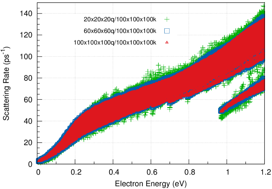
Figure 4: Convergence analysis of the scattering rate of Si at 300K due to el-ph coupling in the Fan-Migdal approximation as a function of the electron energy. The calculation has been performed on different q meshes, namely, $(20)^{3}$ (green crosses), $(60)^{3}$ (blue squares), $(100)^{3}$ (red dots) q-meshes in the first W-F interpolation, while keeping fixed the number of irreducible k points in the second plane-waves interpolation, leading to $(100)^{3}$ k-mesh.

Fig. 4 shows how the scattering rate aproaches convergence by increasing the mesh size of W-F interpolation, from $(20)^{3}$ to $(100)^{3}$ ${\bf{q}}$ points, while keeping the number of irreducible points fixed at $5216$ ${\bf{k}}$ points. The second interpolation by star functions leads into a converged grid with $(100)^{3}$ ${\bf{k}}$ points. Fig. 5 shows the difference in scattering rates calculated by different approaches, namely, different parameters in the second plane-waves interpolation (PWI), over equivalent meshes. The analysis shows that the accompanying error due to the increase in $M$ decreases by enlarging the number of irreducible points, $n_{{\bf{\bar{k}}}}$ (see main text). Moreover, the difference between scattering rates calculated over $(100)^{3}$ ${\bf{q}}$/ $1661$ ${\bf{k}}$ points expanded by using $M=5$ to reach $(100)^{3}$ ${\bf{k}}$-mesh and data from $(100)^{3}$ ${\bf{q}}$/ $256$ ${\bf{k}}$ points expanded by using $M=30$ to reach $(100)^{3}$ ${\bf{k}}$-mesh, is within $\approx\pm 6\%$. For the remaining, the difference between the data points is about the same, within $\approx\pm 3\%$.

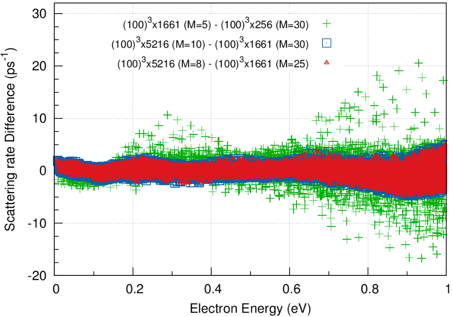
Figure 5: Difference between scattering rates computed by using different parameters in the second plane-waves interpolation, over equivalent meshes. Green crosses correspond to the difference between scattering rates calculated over $(100)^{3}$ q/ $1661$ k points expanded by using $M=5$ to reach $(100)^{3}$ k-mesh and data from $(100)^{3}$ q/ $256$ k points expanded by using $M=30$ to reach $(100)^{3}$ k-mesh. Blue squares correspond to the difference between scattering rates calculated over $(100)^{3}$ q/ $5216$ k points expanded by using $M=10$ to reach $(180)^{3}$ k-mesh and data from $(100)^{3}$ q/ $1661$ k points expanded by using $M=30$ to reach $(180)^{3}$ k-mesh. Red dots correspond to the difference between scattering rates calculated over $(100)^{3}$ q/ $5216$ k points expanded by using $M=8$ to reach $(160)^{3}$ k-mesh and data from $(100)^{3}$ q/ $1661$ k points expanded by using $M=25$ to reach $(160)^{3}$ k-mesh.

Appendix C Calculation of electron self-energy and thermoelectric properties

The expression for the imaginary part of electronic self-energy due to el-ph coupling in the Fan-Migdal approximation can be derived from quantum field theoryGiustino (2017) and it is expressed as

$$\begin{split}\Sigma^{\prime\prime}_{n,{\bf{k}}}(\omega,T)=\pi\sum_{m,\beta}\int_{BZ}\frac{d{\bf{q}}}{\Omega_{BZ}}|g_{mn,\beta}({\bf{k},{\bf{q}}})|^{2}\\ \times\Bigg{[}\left[n_{{\bf{q}}\beta}(T)+f_{m{\bf{k}}+{\bf{q}}}\right]\delta(\omega-(\epsilon_{m{\bf{k}}+{\bf{q}}}-\epsilon_{F})+\omega_{{\bf{q}}\beta})\\ +[n_{{\bf{q}}\beta}(T)+1-f_{m{\bf{k}}+{\bf{q}}}]\delta(\omega-(\epsilon_{m{\bf{k}}+{\bf{q}}}-\epsilon_{F})-\omega_{{\bf{q}}\beta})\Bigg{]}\leavevmode\nobreak\ ,\end{split}$$ (10)

where $n_{{\bf{q}}\beta}(T)$ and $f_{m{\bf{k}}+{\bf{q}}}$ are the Bose-Einstein and the Fermi-Dirac distributions, $\Omega_{BZ}$ is the BZ volume, $m$ and $n$ are the corresponding electronic states, while $\beta$ represents the phonon branch, $\epsilon_{m{\bf{k}}+{\bf{q}}}$ are the electronic eigenenergies of the state $m{\bf{k}}+{\bf{q}}$ and $\omega_{{\bf{q}}\beta}$ are the corresponding eigenfrequencies with wavevector ${\bf{q}}$ and phonon branch $\beta$. Basically, from the first W-F interpolation we can get $f({\bf{\bar{k}}})=\Sigma^{\prime\prime}_{n,{\bf{\bar{k}}}}(\omega,T)$, over the irreducible points, which will be interpolated throughout the whole BZ by star functions, resulting in $\Sigma^{\prime\prime}_{n,{\bf{k^{\prime}}}}(\omega,T)$ over denser ${\bf{k^{\prime}}}$ grids.

$\Sigma^{\prime\prime}$ is directly related to the scattering rate, that is, inversely proportional to the relaxation time

$$\frac{1}{\tau_{n,{\bf{k}}}}=2\Sigma^{\prime\prime}_{n,{\bf{k}}}(\omega=0,T)\leavevmode\nobreak\ ,$$ (11)

which enters in kinetic transport equations. Indeed, the kinetic coefficient tensors can be expressed through

$$\Lambda^{(\alpha)}(\mu;T)=e{{}^{2}}\int\Xi(\epsilon,\mu,T)(\epsilon-\mu)^{\alpha}\left(-\frac{\partial f^{(0)}(\mu;\epsilon,T)}{\partial\epsilon}\right)d\epsilon\leavevmode\nobreak\ ,$$ (12)

where $\mu$ is the chemical potential and $\Xi(\epsilon,\mu,T)$ is the transport distribution kernel given by

$$\Xi(\epsilon,\mu,T)=\int\sum_{n}{{\bf{v}}_{n,{\bf{k}}}\otimes{\bf{v}}_{n,{\bf{k}}}{\tau}_{n,{\bf{k}}}}(\mu,T)\delta(\epsilon-\epsilon_{n,{\bf{k}}})\frac{d{\bf{k}}}{8\pi^{3}}\leavevmode\nobreak\ ,$$ (13)

with ${\bf{v}}_{n,{\bf{k}}}$ being the electron velocity. From both experimental conditions of zero temperature gradient ($\nabla T=0$) and zero electric current, the kinetic coefficient tensors can be identified with the electrical conductivity tensor, $\sigma=\Lambda^{(0)}$, the Seebeck coefficient tensor, $S=(eT)^{-1}\Lambda^{(1)}/\Lambda^{(0)}$, and the charge carrier contribution to thermal conductivity tensor, $\kappa_{e}=(e^{2}T)^{-1}\left({\Lambda^{(1)}\cdot{\Lambda^{(0)}}^{-1}}\cdot{\Lambda^{(1)}}-\Lambda^{(2)}\right)$. Consequently, once we have $\tau_{n,{\bf{k}}}$ from Eq. (11), we can compute the electrical conductivity, the Seebeck coefficient, Lorenz function and the charge carrier contribution to thermal conductivity from the solution of Eq. (13) and Eq. (12). Note that the both bandstructure and phonon dispersion have also been interpolated by the method presented in the main text over the same grid as electron self-energy. Indeed, we have implemented these equations on top of the BoltzTraP code,Madsen and Singh (2006) from which we can obtain these transport properties directly from first principles.

Appendix D Scattering by ionized impurities

For the calculation of thermoelectric transport properties of $n$- and $p$-type Si polycrystals, we have also considered the scattering by ionized impurities. Such scattering has been treated theoretically by Brooks and Herring (B-H)Brooks (1955); Chattopadhyay and Queisser (1981) by considering a screened Coulomb potential, the Born approximation for the evaluation of transition probabilities and neglecting perturbation effects of the impurities on the electron energy levels and wave functions. In the B-H theory the electron is scattered independently by dilute concentrations of ionized centers randomly distributed in the semiconductor.

The per-unit-time transition probability for the scattering of charge carriers by ionized impurities can be given in the plane-wave approximation as

$$W({\bf{k}}|{\bf{{k}^{\prime}}})=\frac{2\pi}{\hbar}\frac{N_{i}}{V}\\ \left|{\int U({\bf{r}})\exp{\left[i({\bf{k}}-{\bf{{k}^{\prime}}};{\bf{r}})\right]}d{\bf{r}}}\right|^{2}\delta(\epsilon({\bf{{k}^{\prime}}})-\epsilon({\bf{k}}))\leavevmode\nobreak\ ,$$ (14)

where $U({\bf{r}})$ is the scattering potential and $N_{i}$ is the ionized impurity concentration.

A long-range Coulomb field, $U(\mbox{\boldmath{$r$}})=e\phi(r)=\pm e^{2}/\zeta r$, with potential $\phi$ at a point $r$ of the crystal is created by the presence of positive (donor) or negative (acceptor) impurity ions, within a medium with dieletric constant $\zeta$. The straightforward application of this field in Eq. (14) leads into a logarithmic divergence, and hence, a screened Coulomb potential has to be considered. From the B-H theory the potential can be expressed in a more rigorous form as $\phi(r)=\pm e/{\zeta r}\left(\exp{\left(-{r}/{r_{0}}\right)}\right)$, where $r_{0}$ is the radius of ion field screening defined by

$$r{{}_{0}}^{-2}({\bf{k}})=\frac{4\pi{e^{2}}}{\zeta{{}_{0}}}\int{-\frac{\partial f_{0}}{\partial\epsilon({\bf{k}})}}g(\epsilon)d\epsilon\leavevmode\nobreak\ ,$$ (15)

where $f^{(0)}(\epsilon)$ is the equilibrium electron distribution function, $\zeta_{0}$ is the static dielectric constant, and $g(\epsilon)$ is the density of states, calculated numerically on an energy grid with spacing $d\epsilon$ sampled over $N_{k}$ ${\bf{k}}$-points

$$g(\epsilon)=\int\sum_{n}\delta(\epsilon-\epsilon_{n,{\bf{k}}})\frac{d{\bf{k}}}{8\pi^{3}}=\frac{1}{\Omega N_{k}}\sum_{n,{\bf{k}}}\frac{\delta(\epsilon-\epsilon_{n,{\bf{k}}})}{d\epsilon}\leavevmode\nobreak\ ,$$ (16)

where $\Omega$ is the volume of the unit cell.

Within the relaxation time approximation for the Boltzmann transport equations, the relaxation time for the scattering of the charge carriers by ionized impurities can be expressed as

$$\tau_{imp}({\bf{k}})=\frac{\hbar\zeta{{}_{0}}{{}^{2}}}{2{\pi}{e^{4}}{N_{i}}F_{imp}({\bf{k}})}{\bf{k}}^{2}\left|\frac{\partial\epsilon({\bf{k}})}{\partial{\bf{k}}}\right|$$ (17)

where

$$F_{imp}({\bf{k}})=ln(1+\eta)-\frac{\eta}{1+\eta}\leavevmode\nobreak\ ,$$ (18)

is the screening function with $\eta=(2{\bf{k}}r_{0})^{2}$. Here, we interpolated $\left|\frac{\partial\epsilon({\bf{k}})}{\partial{\bf{k}}}\right|$ within Eq. (17) by using the plane-waves interpolation (see the main text) and used Mathiessen’s rule to consider both the scattering by ionized impurities and phonons.

Appendix E Calculation of phonon-assisted optical absorption

To calculate the phonon-assisted absorption coefficient, we use the Fermi’s golden rule expressionBassani and Parravicini (1975); Noffsinger et al. (2012):

$$\alpha(\omega)=2\frac{4\pi^{2}e^{2}}{\omega cn_{r}(\omega)}\frac{1}{\Omega}\frac{1}{N_{{\bf{k}}}N_{{\bf{q}}}}\sum_{\beta ij{\bf{k}}{\bf{q}}}|{\mbox{\boldmath{$\lambda$}}}\cdot({\bf{S_{1}}}+{\bf{S_{2}}})|^{2}$$ (19)

$$\times P\delta(\epsilon_{j,{\bf{k}}+{\bf{q}}}-\epsilon_{i,{\bf{k}}}-\hbar\omega-\pm\hbar\omega_{\beta{\bf{q}}})\leavevmode\nobreak\ ,$$

with

$${\bf{S_{1}}}({\bf{k}}{\bf{q}})=\sum_{m}\frac{{\bf{v}}_{im}({\bf{k}})g_{mj,\beta}({\bf{k}},{\bf{q}})}{\epsilon_{m,{\bf{k}}}-\epsilon_{i{\bf{k}}}-\hbar\omega+i\Gamma_{m,{\bf{k}}}}\leavevmode\nobreak\ ,$$ (20)

$${\bf{S_{2}}}({\bf{k}}{\bf{q}})=\sum_{m}\frac{g_{im,\beta}({\bf{k}},{\bf{q}}){\bf{v}}_{mj}({\bf{k}}+{\bf{q}})}{\epsilon_{m,{\bf{k}}+{\bf{q}}}-\epsilon_{i{\bf{k}}}\pm\hbar\omega_{\beta{\bf{q}}}+i\Gamma_{m,{\bf{k}}+{\bf{q}}}}\leavevmode\nobreak\ ,$$ (21)

and

$$P=(n_{\beta{\bf{q}}}+\frac{1}{2}\pm\frac{1}{2})(f_{i{\bf{k}}}-f_{j,{\bf{k}}+{\bf{q}}})\leavevmode\nobreak\ .$$ (22)

In these equations, $\omega$ is the photon frequency, $c$ is the speed of light, $n_{r}$ is the refractive index (for silicon we used $n_{r}=3.4$), and $\lambda$ is the photon polarization. ${\bf{S_{1}}}$ and ${\bf{S_{2}}}$ are the two possible ways for the indirect absorption process, while $P$ is related to the carrier and phonon statistics. For calculations of Si, the DFT band gap and all conduction bands have been shifted up by $0.7$$\mathrm{eV}$ to simulate experimental gap. Our calculations have been carried out over $(60)^{3}$q/$(40)^{3}$k meshes. It took $\approx 36$ minutes to perform the calculation by using our dual interpolation method on $8$ CPU cores at the Odyssey cluster (Harvard University).

References

- Giustino (2017) F. Giustino, Reviews of Modern Physics 89, 015003 (2017).
- Marini (2008) A. Marini, Physical Review Letters 101, 106405 (2008).
- Park et al. (2007) C.-H. Park, F. Giustino, M. L. Cohen, and S. G. Louie, Physical Review Letters 99, 086804 (2007).
- Restrepo et al. (2009) O. Restrepo, K. Varga, and S. Pantelides, Applied Physics Letters 94, 212103 (2009).
- Margine and Giustino (2014) E. Margine and F. Giustino, Physical Review B 90, 014518 (2014).
- Fiorentini and Bonini (2016) M. Fiorentini and N. Bonini, Physical Review B 94, 085204 (2016).
- Wang et al. (2011) Z. Wang, S. Wang, S. Obukhov, N. Vast, J. Sjakste, V. Tyuterev, and N. Mingo, Physical Review B 83, 205208 (2011).
- Noffsinger et al. (2012) J. Noffsinger, E. Kioupakis, C. G. Van de Walle, S. G. Louie, and M. L. Cohen, Physical Review Letters 108, 167402 (2012).
- Boukai et al. (2011) A. I. Boukai, Y. Bunimovich, J. Tahir-Kheli, J.-K. Yu, W. A. Goddard III, and J. R. Heath, in Materials For Sustainable Energy: A Collection of Peer-Reviewed Research and Review Articles from Nature Publishing Group (World Scientific, 2011) pp. 116–119.
- Strasser et al. (2004) M. Strasser, R. Aigner, C. Lauterbach, T. Sturm, M. Franosch, and G. Wachutka, Sensors and Actuators A: Physical 114, 362 (2004).
- Baroni et al. (2001) S. Baroni, S. De Gironcoli, A. Dal Corso, and P. Giannozzi, Reviews of Modern Physics 73, 515 (2001).
- Li (2015) W. Li, Physical Review B 92, 075405 (2015).
- Giustino et al. (2007) F. Giustino, M. L. Cohen, and S. G. Louie, Physical Review B 76, 165108 (2007).
- Marzari and Vanderbilt (1997) N. Marzari and D. Vanderbilt, Physical Review B 56, 12847 (1997).
- Braunstein et al. (1958) R. Braunstein, A. R. Moore, and F. Herman, Physical Review 109, 695 (1958).
- Fetter and Walecka (2012) A. L. Fetter and J. D. Walecka, Quantum theory of many-particle systems (Courier Corporation, 2012).
- Pick et al. (1970) R. M. Pick, M. H. Cohen, and R. M. Martin, Physical Review B 1, 910 (1970).
- Poncé et al. (2014) S. Poncé, G. Antonius, P. Boulanger, E. Cannuccia, A. Marini, M. Côté, and X. Gonze, Computational Materials Science 83, 341 (2014).
- Chadi and Cohen (1973) D. Chadi and M. L. Cohen, Physical Review B 8, 5747 (1973).
- Shankland (1971) D. G. Shankland, in Computational Methods in Band Theory (Plenum, New York, 1971) p. 362.
- Koelling and Wood (1986) D. Koelling and J. Wood, Journal of Computational Physics 67, 253 (1986).
- Pickett et al. (1988) W. E. Pickett, H. Krakauer, and P. B. Allen, Physical Review B 38, 2721 (1988).
- Sun et al. (2012) Y. Sun, S. Boggs, and R. Ramprasad, Applied Physics Letters 101, 132906 (2012).
- Qiu et al. (2015) B. Qiu, Z. Tian, A. Vallabhaneni, B. Liao, J. M. Mendoza, O. D. Restrepo, X. Ruan, and G. Chen, EPL (Europhysics Letters) 109, 57006 (2015), arXiv:1409.4862 (2014).
- Rideau et al. (2011) D. Rideau, W. Zhang, Y. Niquet, C. Delerue, C. Tavernier, and H. Jaouen, in 2011 International Conference on Simulation of Semiconductor Processes and Devices (SISPAD) (IEEE, New York, 2011) pp. 47–50.
- Madsen and Singh (2006) G. K. Madsen and D. J. Singh, Computer Physics Communications 175, 67 (2006).
- Poncé et al. (2016) S. Poncé, E. R. Margine, C. Verdi, and F. Giustino, Computer Physics Communications 209, 116 (2016).
- Giannozzi et al. (2009) P. Giannozzi et al., Journal of Physics: Condensed Matter 21, 395502 (2009).
- Perdew et al. (1996) J. P. Perdew, K. Burke, and M. Ernzerhof, Physical Review Letters 77, 3865 (1996).
- Scherpelz et al. (2016) P. Scherpelz, M. Govoni, I. Hamada, and G. Galli, Journal of chemical theory and computation 12, 3523 (2016).
- Mostofi et al. (2008) A. A. Mostofi, J. R. Yates, Y.-S. Lee, I. Souza, D. Vanderbilt, and N. Marzari, Computer physics communications 178, 685 (2008).
- Brooks (1955) H. Brooks, in Advances in electronics and electron physics, Vol. 7 (Elsevier, 1955) pp. 85–182.
- Chattopadhyay and Queisser (1981) D. Chattopadhyay and H. Queisser, Reviews of Modern Physics 53, 745 (1981).
- Bassani and Parravicini (1975) F. Bassani and G. P. Parravicini, Electronic States and Optical Transitions in Solids (Pergamon press, New York, 1975).