Incremental Calibration of Architectural Performance Models with Parametric Dependencies

Abstract

Architecture-based Performance Prediction (AbPP) allows evaluation of the performance of systems and to answer what-if questions without measurements for all alternatives. A difficulty when creating models is that Performance Model Parameters (PMPs, such as resource demands, loop iteration numbers and branch probabilities) depend on various influencing factors like input data, used hardware and the applied workload. To enable a broad range of what-if questions, Performance Models (PMs) need to have predictive power beyond what has been measured to calibrate the models. Thus, PMPs need to be parametrized over the influencing factors that may vary.

Existing approaches allow for the estimation of parametrized PMPs by measuring the complete system. Thus, they are too costly to be applied frequently, up to after each code change. They do not keep also manual changes to the model when recalibrating.

In this work, we present the Continuous Integration of Performance Models (CIPM), which incrementally extracts and calibrates the performance model, including parametric dependencies. CIPM responds to source code changes by updating the PM and adaptively instrumenting the changed parts. To allow AbPP, CIPM estimates the parametrized PMPs using the measurements (generated by performance tests or executing the system in production) and statistical analysis, e.g., regression analysis and decision trees. Additionally, our approach responds to production changes (e.g., load or deployment changes) and calibrates the usage and deployment parts of PMs accordingly.

For the evaluation, we used two case studies. Evaluation results show that we were able to calibrate the PM incrementally and accurately.

I Introduction

In many application domains, software is nowadays developed iteratively and incrementally, e.g., following agile practices. This means that there usually is no dedicated architecture design phase, but architectural design decisions are made continuously throughout the development. For performance analysis, this means that there is not a single point in time at which the performance analysis is carried out, but a performance analysis is required whenever performance-critical architecture design decisions have to be made.

In such iterative and incremental development projects, developers typically use Application Performance Management (APM) [17, 9] to assess the current performance of their software. However, APM cannot predict the impact of design decisions or to answer scalability and sizing questions in a large and distributed environment, where the resources may not be accessible and a huge amount of load generators would be needed.

Software performance engineering [4, 43] uses models to assess the performance of a software system. It supports the evaluation of various architecture, design, implementation and workload choices. Compared to APM, such model-based performance prediction [7] allows to predict future alternatives before implementing them [43]. In particular, Architecture-based Performance Prediction (AbPP) approaches [42] reflect the architecture of the software system in a Performance Model (PM) in order to easily study design alternatives [36].

The problem of AbPP in iterative-incremental development is that modelling is a time-consuming process. In particular, calibrating Performance Model Parameters (PMPs) (e.g., Resource Demands (RDs), branch probabilities, and loop counts) is challenging, because the PMPs may depend on impacting factors such as input data, properties of required resources or usage profile. Ignoring these so-called parametric dependencies [8]) will lead to inaccurate performance predictions. Thus, keeping the PM and in particular the parametrized PMPs consistent with the iteratively and incrementally evolving source code over time requires repeated manual effort.

To address the high effort to create performance models when source code is available, researchers have suggested several approaches to extract PMs automatically. However, most of these approaches [10, 48, 3, 33, 44] have three shortcomings: First, they require instrumentation and execution of the whole system under study to extract the PM, which causes a high overhead and is not feasible at high frequency, e.g., after each source code commit. Second, they do not consider parametric dependencies. Notable exceptions are the approach by Krogmann et al. [30, 29] or Grohmann et al. [15], which also extract parametric dependencies (but monitor the whole system to calibrate the model without keeping the manual changes). Third, they reconstruct the whole architectural PM from scratch. Thus, they cannot keep manual changes of the architecture model, which is problematic if the architecture model shall be used as an architecture knowledge base and is enhanced manually with e.g. the rationale of architecture decisions [28].

In this paper, we present our approach, called Continuous Integration of the Performance Model (CIPM), to incrementally extract and calibrate architecture-level PMs with parametric dependencies after each source code commit. Our approach builds upon the Palladio approach [42] for modelling and simulating architecture-level PMs. We have extended an incremental extraction of such architectural PMs [31] with incremental calibration that considers the parametric dependencies and is based on adaptive monitoring. The goal of the approach is to keep the PM up-to-date automatically to allow AbPP. An initial version of this idea has been presented in a workshop publication [37] without evaluation.

The contributions of our paper are twofold:

1. Incremental Dev-time calibration: We propose a novel incremental calibration at Development time (Dev-time) that responds to source code changes by adaptive instrumentation of the changed parts of the code and uses the resulting measurements from performance tests or the production system to estimate the PMPs incrementally.

   For this purpose, we propose a novel incremental Resource Demand Estimation (RDE) that is based on adaptive monitoring. Our calibration uses statistical analysis to learn potential dependencies, e.g., regression analysis for resource demands and decision trees for the estimation of branch transitions.

2. Model-based DevOps pipeline: We extend agile DevOps practices [11] to integrate the CIPM activities and thus to reduce the effort for AbPP. To do so, we propose a model-based DevOps pipeline and implement a part of it. In addition to the above-mentioned incremental Dev-time calibration, we also include an existing approach for calibration at Operation time (Ops-time) in the pipeline. This Ops-time calibration responds to changes in deployment and usage profile and updates the respective parts of the PM. We include also prototypical self-validation steps.

We evaluate our contributions using two case studies [22, 25]. The evaluation confirmed that the incremental calibration was able to detect parametric dependencies while significantly reducing the monitoring overhead. Moreover, we showed that the calibrated performance models are accurate by comparing the simulation results with monitored data.

The next section gives an overview of the foundations. Section III introduces a motivating example. The overall CIPM process is presented in Section IV. Section V describes how to embed CIPM in the model-based DevOps pipeline. The next three sections provide detail on the CIPM activities: Section VI presents the adaptive instrumentation, Section VII describes the incremental calibration and Section VIII describes how we estimate the parametric dependencies. Our evaluations are discussed in Section IX. The related work follows in Section X. The paper ends with our conclusions and future work (Section XI).

II Foundations

II-A Palladio

Palladio is an approach to model and simulate architecture-level PMs and has been used in various industrial projects [42, 8]. Within Palladio, the so-called Palladio Component Model (PCM) defines a language for describing PMs: the static structure of the software (e.g. components and interfaces), the behavior, the required resource environment, the allocation of software components and the usage profile. The PCM Service Effect Specification (SEFF) [8] describes the behavior of a component service on an abstract level using different control flow elements: internal actions (a combination of internal computations that do not include calls to required services), external call actions (calls to required services), loops and branch actions. SEFF loops and branch actions include at least one external call. Other loops and branches in the service implementation are ignored and combined into the internal actions to increase the level of abstraction.

To predict the performance measures (response times, central processing unit (CPU) utilization and throughput) the architects have to enrich the SEFFs with PMPs. Examples of PMPs are resource demands (processing amount that internal action requests from a certain active resource, such as a CPU or hard disk), the probability of selecting a branch, the number of loop iterations and the arguments of external calls.

Palladio uses the stochastic expression (StoEx) language [26] to define PMPs as expressions that contain random variables or empirical distributions. StoEx allows parameter characterization (e.g. determining NUMBER_OF_ELEMENTS, VALUE, BYTESIZE and TYPE) and to express calculations and comparisons (e.g., file.BYTESIZE$<=$5*max.VALUE).

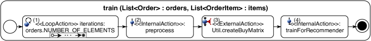
Figure 1: The behavior of TeaStore’s ”Recommender.train” service using SEFF

II-B Co-evolution approach with Vitruvius

The co-evolution approach of Langhammer et al. [32, 31] helps software developers and architects to keep the architecture model and the code consistent when their software system evolves. It defines change-driven consistency preservation rules that propagate changes in source code to the architecture model and vice versa using model-based transformations.

These rules are defined based on Vitruvius [27, 12], a view-based framework that encapsulates the heterogeneous models of a system and the semantic relationships between them in a Virtual Single Underlying Model (VSUM) in order to keep them consistent. Vitruvius defines mappings and reactions languages that describe consistency rules on the metamodel-level. These rules describe the consistency repair logic for each kind of changes, i.e., which and how the artifacts of a metamodel have to be changed to restore the consistency after a change in a related metamodel has occurred.

Using Vitruvius, Langhammer et al. implemented their approach to keep Java source code (using an intermediate model [18]) and a PCM model consistent. The defined consistency rules update the structure of a PCM model (i.e. components and interfaces) and its behavior (in term of SEFFs, but without PMPs) as a reaction to changes in the source code. Similarly, changes in PCM model are propagated to the Java source code.

II-C Kieker

Kieker [23] is an APM tool that captures and analyzes execution traces from distributed software systems. It allows one to describe specific probes (data structures of the monitored information) using the Instrumentation Record Language (IRL) [6]. It also supports dynamic and adaptive monitoring by activating or deactivating probes during run time.

II-D iObserve

iObserve [21] aims to increase the human comprehensibility of run-time changes by updating an architecture model accordingly. The authors defined specific monitoring records using IRL and map the resulting measurements to the corresponding parts in the PCM using the so-called Run-time Architecture Correspondence Meta-Model (RAC) [20]. iObserve detects changes concerning the deployment and the user behavior and updates the related parts of the PCM to analyze performance and privacy aspects [19]. However, iObserve does not support updating component behavior models (SEFFs) with PMPs.

III Running Example

We introduce a motivating example that illustrates our approach and was used to evaluate it (see Sec. IX). The example is part of the TeaStore case study [25]: a website to buy different kinds of tea. In this case study, the Recommender component is responsible for calculating the recommendations for a certain shopping cart using the services ‘train’ and ‘recommend’. The ‘train’ service derives information from the previous orders and prepares the data for the ‘recommend’ service. Because there are different strategies to recommend a list of related items, the developers implemented four versions of ‘recommend’ and ’train’ along different development iterations. These implementations have different performance characteristics. Performance tests or monitoring can be used to discover these characteristics for the current state, i.e., for the current deployment and the current workload. However, predicting the performance for another state (e.g., different deployment or workload) is expensive and challenging because it requires setting up and performing several tests for each implementation alternative. In our example, answering the following questions is challenging based on APM: “Which implementation would perform better if the load or the deployment is changed?” or “How well does the ’train’ service perform during yet unseen workload scenarios?” An example for the latter question would be an upcoming offer of discounts, where architects expect an increased number of customers and also a changed behavior of customers in that each customer is expected to order more items.

AbPP can answer these questions faster using simulations instead of the expensive tests if an up-to-date PM is available.

Regardless how the model will be built and updated (reverse engineering extraction or manual/ automatic update), all available approaches recalibrate the whole model by monitoring all parts of the source code instead of recalibrating only the model parts affected by the last changes in source code. For example, the changes in the implementation of ’train’ belong to the last part of the code which is represented as an internal action ‘trainForRecommender’ by modelling the behaviour using SEFF (see Fig. 1). This means that these changes have only impact on the RD of ‘trainForRecommender’ and all other PMPs are valid (e.g., RD of preprocessor internal action). Recalibrating the whole PMPs loses potential previous manual changes and causes unnecessary monitoring overhead. Additionally, not all the available approaches detect the parametric dependencies (e.g., the RD of ‘trainForRecommender’ is related to the number of ordered items).

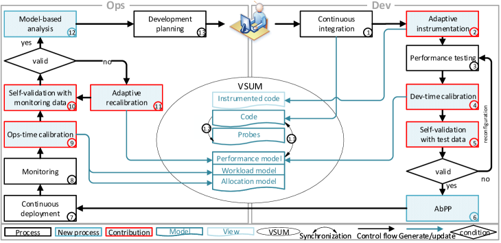
Figure 2: Model-based DevOps pipeline

IV Continuous Integration of Performance Model

This section provides an overview of the CIPM approach, before describing how it is embedded in a continuous software engineering approach in Section V and before providing more details on the CIPM activities in Sections VI-VII.

Our approach CIPM incrementally extracts and calibrates architecture-level PMs with parametric dependencies after each source code commit. To do so, CIPM updates the PM continuously to keep it consistent with the running system, i.e., the deployed source code and the last measurements.

CIPM consists of four main activities:

1. Performance model update and adaptive instrumentation: CIPM analyzes the source code changes, updates the architectural PM and static behavior model based on the co-evolution approach [31] and instruments the changed parts of code to calibrate the new/ updated related parts of the architecture as will be discussed in Section VI.

2. Monitoring: CIPM collects the required measurements either during testing or executing the system in production.

3. Incremental calibration of PM (Sec. VII): CIPM performs the Dev-time calibration of behavior, i.e., PMPs (Sec. VII-A) considering the parametric dependencies (Sec. VIII) and the Ops-time calibration, i.e., updating the deployment and usage parts of PM (Sec. VII-B).

4. Self-validation: CIPM automatically starts a simulation and calculates the variation between the simulation results and the monitoring data to show the estimation error before performing AbPP.

To realize these four activities, CIPM extends the co-evolution approach with a monitoring process to keep the PM consistent with the last up-to-date measurements. The static structure and behavior update of PM is already provided by the co-evolution approach. For the adaptive instrumentation, we (a) extend the VSUM with an Instrumentation Model (IM) that describes and manages the instrumentation points and (b) define the consistency rules between the IM and source code. The rules define how Vitruvius has to respond to the changes in code by adaptive instrumentation of the changed parts with predefined monitoring probes. For the monitoring, we (c) define a Measurements Model (MM) that describes the resulting monitoring records. These records belong to specific types that are responsible for collecting the necessary monitoring information to calibrate the SEFF elements. Finally, for the incremental calibration and estimation of parametric dependencies, we (d) define the consistency rules between MM and PM, which analyze the monitoring data, calibrate the PMPs and update the deployment and usage parts of PM.

With our approach, we can also handle overlapping commits that occur while the monitoring and calibration of a previous commit are still ongoing by managing multiple copies of the PM and keeping track of which model instance belongs to which version of the source code.

V The Model-based DevOps Pipeline

DevOps practices aim to close the gap between the development and operations and to integrate them into one reliable process. We extend the DevOps practices to integrate and automate the CIPM in a Model-based DevOps (MbDevOps) pipeline. This enables AbPP during DevOps-oriented development. The next paragraphs explain the pipeline processes. The lower case numbers refer to the process’s number in Fig. 2.

The MbDevOps pipeline starts on the “development” side with $continuous\>integration_{1}\>(CI)$ process [40] that merges the source code changes of the developers (cf.  Fig. 2). Vitruvius responds to the changes in source code with the first CIPM activity: $updating\>the\>architectural\;PM_{1.1}$ and $generating\>the\>required\>instrumentation\>points\>in\>IM_{1.2}$ (cf. Sec. II-B). Next, $adaptive\>instrumentation_{2}$ instruments the changed parts of source code using the instrumentation points from IM (Sec. VI). The following process is the $performance\>testing_{3}$, which integrates the second CIPM activity ’Monitoring’ to generate the necessary measurements for calibration. The pipeline divides the measurements into training and validation set. Afterwards, the $Dev{-}time\>calibration_{4}$ (the first part of 3 CIPM activity) enriches the PM with PMPs using the training set. Section VII describes the incremental calibration process whereas Section VIII explains how we parametrize the PMPs with the influencing input parameters. After the calibration, the pipeline starts the $self{-}validation\>with\>test\>data_{5}$ process (the 4 CIPM activity), which uses the validation set to evaluate the calibration accuracy. If the model is deemed accurate, developers can use the resulting PM to answer the performance questions using $AbPP_{6}$. If not, they can change the test configuration to recalibrate PM. Answering the performance questions using AbPP instead of the test-based performance prediction reduces both the effort and cost of setting up the test environment to perform this prediction.

The “operations” side of Figure 2 starts on the $continuous\>deployment_{7}$ in the production environment. CIPM $Monitoring_{8}$ in the production environment generates the required run-time measurements for the next process: $Ops{-}time\>calibration_{9}$ (the second part of the 3 CIPM activity). The ops-time calibration calibrates and updates both usage model and deployment model (Sec. VII-B). Next, the $self{-}validation\>with\>monitoring\>data_{10}$ (the 4 CIPM activity) validates the estimated PMPs. If the PM is not accurate enough, the $adaptive\>recalibration_{11}$ process (Sec. VII) recalibrates the inaccurate model parts using monitoring data. Finally, the developers can perform more $model-based\>analysis_{12}$ on the resulting model, e.g., model-based auto scaling. Additionally, having an up-to-date descriptive PM supports the $development$ $planning_{13}$. This is due to the advantages of models: increasing the understandability of the current version, modelling and evaluating design alternatives and answering what-if questions.

VI Adaptive Instrumentation

The goal is to instrument the parts of source code, which have been changed and their changes may affect the validity of related PMPs. In our running example, only the source code of ’trainForRecommender’ is instrumented to provide the required measurements to update the RD, whereas there is no need to instrument the loop or the code of ‘preprocess’, because these parts of code are not changed, consequently the old estimations of the PMPs remain valid.

To automate the adaptive instrumentation, we use the consistency rules between the source code model and IM, which responds to changes in method body (e.g., adding/ updating statements) by instrumenting the related parts. The rules reconstruct the SEFF using a reverse engineering tool [29] and map code statements to their SEFF element (e.g., internal actions). Then, they create the required probes (e.g., service probe, internal action probe, loop probe or branch probe) that refer to the SEFF elements whose code statements have been changed. We define the following monitoring record types that are related to the aforementioned probe types using IRL (cf. Section II-C).

• Service call record to monitor the following:
  - the input parameters properties (e.g., type, value, number of list elements, etc.) that should be considered later as candidates for parametric dependency investigation,
  - the caller of this service execution to learn the parametric dependency between the input parameters of both caller and callee services.
  - the allocation context that captures where the component offering this service is deployed.

• Internal-action record type to monitor the response time of the internal actions.

• Loop record to monitor the number of loop iterations.

• Branch record to monitor the selected branch.

More details about the records types are in [24, Chapter 4.3.3].

Finally, we implemented a model-based instrumentation to generate the instrumented source code as a Vitruvius view. This view combines the information from two models: the source code model and the IM. The instrumentation starts with generating the instrumentation code for each probe in the IM according to the probe type. Then it injects the instrumentation codes into a copy of the source code. To detect the correct places for the instrumentation codes, the instrumentation process uses the relations stored in Vitruvius correspondence model, i.e., the relation between probes and SEFF elements, the relation between SEFF elements and their source code statements and relation between the original source code and the generated copy (instrumented source code).

VII Incremental Calibration

The following subsections explain the calibration types.

VII-A Dev-time calibration

The Dev-time changes that we consider in this paper are the source code changes that may have an impact on performance, i.e., changes in a method body.

On one hand the incremental calibration of the SEFF branches, loops or external call arguments requires only to instrument the related source code and to analyze the resulting measurements (e.g., loop iteration number, the selected branch transition, and the values of external call parameters). The goal of this analysis is to detect whether there are dependencies to the service input parameters and express these PMPs sequentially as stochastic expression (cf. Sections VIII-B, VIII-C and VIII-D).

On the other hand, the incremental calibration of the internal actions with Resource Demand (RD) is challenging because we aim to estimate the RD of internal actions incrementally without high monitoring overhead. The existing RDE approaches either estimate the RDs at the service level [45] or require expensive fine-grained monitoring [5, 30]. Therefore, we propose in the following paragraph a light-weight RDE process that is based on adaptive instrumentation and monitoring to allow for an incremental RDE.

Our incremental RDE aims to estimate the RDs in the case of adaptive monitoring, i.e., monitoring the changed parts of source code. In our running example, monitoring the code of ‘trainForRecommender’ to reestimate its RD. For this goal, we extend the approach of Brosig et al. [5].

Basis: Non-incremental estimation of resource demands

Brosig et al. approximate the RDs with measured response times in the case of low resource utilization, typically 20%. Otherwise, they estimate the RD of internal action $i$ (a part of SEFF, see Section II-A) for resource $r$ ($D_{i,r}$) based on service demand law [39] shown in equation (1). Here, $U_{i,r}$ the average utilization of resource r due to executing internal action $i$ and $C_{i}$ is the total number of times that internal action $i$ is executed during the observation period of fixed length $T$:

$$D_{i,r}=\frac{U_{i,r}}{{C_{i}}/{T}}=\frac{U_{i,r}\cdot T}{C_{i}}$$ (1)

Brosig et al. measure the $C_{i}$ and estimate $U_{i,r}$ by using the weighted response time ratios of the total resource utilization, which is not applicable in our adaptive case where not all internal actions are monitored. Therefore, we extend their approach to estimate $U_{i,r}$ and as a result $D_{i,r}$ based on the available measurements and the old RDs estimations.

Incremental estimation of resource demands

Our new approach distinguishes internal actions into two categories based on whether they have been modified in the source code commit preceding the incremental calibration. We denote internal actions whose corresponding code regions have been modified in the preceding source code commit as Monitored Internal Actions (MIAs), e.g., ’trainForRecommender’ in our running example, – for these code regions, the consistency rules will generate instrumentation probes and the adaptive monitoring produce monitoring results. We denote internal actions whose corresponding code regions have not been changed in the preceding source code commit as Not Monitored Internal Actions (NMIAs), e.g., ’preprocess’ in our running example – monitoring data for these code regions has already been observed in a previous iteration and, consequently, we have already an estimation of their RDs.

Based on the fact that the total utilization $U_{r}$ is measurable and the utilization due to executing NMIAs can be estimated based on the old estimations of RDs, we can estimate $U_{r,MIAs}$ and estimate the RD for each internal action $i\in MIAs$ accordingly as it will be explained in following paragraphs.

To estimate ($U_{r,NMIAs}$), we estimate which internal actions $nmi\in NMIAs$ are processed in this interval and how many times $nmi$ are called ($C_{nmi}$). For that, we analyze the service call records (see Section VI) to determine which services are called in an observation period $T$ and which parameters are passed. Then we traverse the service’s control flows (i.e. their SEFFs) to get NMIAs and predict their RD using the input parameters. This requires evaluating branches and loops of the control flow to decide which branch transition we have to follow and how many times we have to handle the inner control flow of loops. Our calibration, adjusts the new or outdated branches and loops using the monitoring data (as will be described in Sections VIII-B and VIII-C) before starting this incremental RDE. Thus, we make sure that we can traverse the SEFFs control flow. Consequently, we can sum up the predicted RDs for all calls of the NMIAs and divide the result by $T$ to estimate the $U_{r,NMIAs}$ based on the utilization law as shown in the equation 2:

$$U_{r,NMIAs}=\frac{\sum\limits_{nmi\in NMIAs}\>\sum\limits_{k\leq C_{nmi}}{D_{nmi_{k},r}}}{T}$$ (2)

Accordingly, we estimate the utilization due to executing the MIAs ($U_{r,MIAs}$) using the measured $U_{r}$ and the estimated $U_{r,NMIAs}$ as shown in equation (3):

$$U_{r,MIAs}=U_{r}-U_{r,NMIAs}$$ (3)

Hence, we can estimate the utilization $U_{i,r}$ due to executing each internal action $i\in MIAs$ using the weighted response time ratios as shown in equation (4), where $R_{i}$ and $C_{i}$ are the average response time of $i$ and its throughput. $R_{j}$ is the average response time of the internal action $j\in MIAs$ and $C_{j}$ is the number of executing it in $T$.

$$U_{i,r}=U_{r,MIAs}.\frac{R_{i}\cdot C_{i}}{\sum\limits_{j\in MIAs}{R_{j}}\cdot C_{j}}$$ (4)

Using $U_{i,r}$ we can estimate the resource demand for $i$ ($D_{i,r}$) based on the service demand law presented in equation (1).

In the case that the host has multiple processors, our approach uses the average of the utilizations as $U_{r}$.

Note that we assume that each internal action is dominated by a single resource. If this is not the case, we have to follow the solution proposed by Brosig et al., to measure processing times of individual execution fragments, so that the measured times of these fragments are dominated by a single resource [5]. To differ between the CPU demands and disk demands, we suggest detecting the disk-based services in the first activity of CIPM using specific notation or based on the used libraries.

VII-B Ops-time calibration

The task of the Ops-time calibration is to update the usage models as well as the deployment model according to the run-time measurements. To achieve that, we use the iObserve approach, which analyzes the measurements and aggregates them to detect changes concerning the deployments and the user behavior. For this, we extended our monitoring records so that all information required by iObserve is available. This allows us to integrate the usage model extraction and the identification of deployments from iObserve. We do not need the RAC from iObserve, because the mapping information is implicitly presented in our monitoring records, e.g., the records that track the execution of a service include explicitly the ID of the associated service in the architectural model.

VIII Parametric dependencies

This work estimates how PMPs depend on input data and their properties (such as number of elements in a list or the size of a file). We begin by estimating the dependencies of branches and loops, because the incremental RDE require traversing the SEFF control flow to estimate the utilization of NMIAs. Currently, we investigate a linear, quadratic, cubic and square root relations using Weka library [16]. However, we are working on optimizing our estimation using genetic algorithms. The following sections explain the analysis that we follow to estimate the parametric dependencies of PMPs.

VIII-A Resource demands

To learn the parametric dependency between the resource demand of an internal action $i$ and input parameters $P$, we first estimate the resource demand on resource $r$ for each combination of the input parameters ($D_{i,r}(P)$) using the proposed incremental RDE as described in Section VII-A.

Second, we adjust the estimated RDs of an internal action using the processing rate of the resource, where it is executed, to extract the resource demand independently of the resource’ processing rate $D_{i}(p)$.

Third, if the input parameters include enumerations, we perform additional analysis to test the relation between RDs and enumeration values using decision tree. If a relation is found, we build a data set for each enumeration value. Subsequently, we perform the regression analysis as it will be described in the following paragraph. Otherwise, we create one data set for each internal action that includes the estimated RDs and their related numeric parameters. The goal is to find the potential significant relations by the regression analysis of the following equation:

$$D_{i}(P)=(a*p_{0}+b*p_{1}+\dotsb+z*p_{n}+$$

$$\qquad\qquad a_{1}*p_{0}^{2}+b_{1}*p_{1}^{2}+\dotsb+z_{1}*p_{n}^{2}+$$

$$\qquad\qquad a_{2}*p_{0}^{3}+b_{2}*p_{1}^{3}+\dotsb+z_{2}*p_{n}^{3}+$$

$$\qquad\qquad\qquad\qquad a_{3}*\sqrt{P_{0}}+b_{3}*\sqrt{p_{1}}+\dotsb+z_{3}*\sqrt{p_{n}}+\textbf{C})\vspace{-0.1cm}$$

$p_{0}$, $p_{1}$.. $p_{n}$ are the numeric input parameters and the numeric attributes of objects that are input parameters.

$a$… $z$, $a_{1}$… $z_{1}$, $a_{2}$… $z_{2}$ and $a_{3}$… $z_{3}$ are the weights of the input parameters and their transformations using quadratic, cubic and square root functions. $C$ is a constant value.

Fourth, we perform the regression analysis algorithm to find the weights of the significant relations and the constant $C$.

Fifth, we replace the constant value $C$ with a stochastic expression that describes the empirical distribution of $C$ value instead of the mean value delivered by the regression analysis. This step is particularly important when no relations to the input parameters are found. In that case, the distribution function will represent the RD of internal action better than a constant value. To achieve that, we iterate on the resulting equation that includes the significant parameters and their weights, to recalculate the value of $C$ for each RD value and their relevant parameters. Then, we build a distribution that represents all measured values and their frequency.

Finally, we build the stochastic expression of RD that may include the input parameters and the distribution of $C$.

VIII-B Loop iterations count

To estimate how the number of loop iterations depends on input parameters, we need both the loop iterations’ count and the input parameters for each service call. To achieve that, we use our loop records that log the loop iterations’ count, every time a loop finishes (see Section VI). These records refer to the service call record that contains the input parameters.

The reason why we use additional records to count loop iterations instead of counting the total amount of enclosing service calls, is that the loop may have a nested branch or loop, which does not allow one to infer the correct count of loop iterations [24].

To estimate the dependency of the loop iteration count on input parameters, we combine the monitored loop iterations with the integer input parameter into one data set. To do so, we filter out all non-integer parameters and take into account their integer properties like number of list elements or size of files. Then, we add transformations (quadratic and cubic) of parameters to the data set to test more relations. Finally, we use regression analysis to estimate the weights of the influencing parameters. Due to the restriction that the loop iterations count is an integer number, we have to ensure, that the output value is always an integer value, which is not always the case. Therefore, we have to approximate the non-integer weights or express them as a distribution of integer values. For instance, we can express the value 1.6 using a Palladio distribution function of an integer variable which takes the value $1$ in $40\%$ of all cases and the value $2$ in $60\%$ of cases. Similar to the fifth step of parametrized RDE in Section VIII-A, we replace the constant value of the resulting stochastic expression with an integer distribution function. This will be especially useful, when no relation to the input parameters is found.

VIII-C Branch transitions

To estimate the parameterized branch transitions, we use the predefined branch monitoring records that log which branch transitions are chosen in addition to a reference to the enclosing service call.

We monitor each branch instead of predicting the selected transition according to the external call execution enclosed in the branch due to potential nested control flows (e.g., nested branches), where we cannot infer the selected transition [24].

The used monitoring records allow us to build a data set for each branch, which includes the branch transitions and the input parameters. To estimate the potential relations, we use the J48 decision tree of the Weka library, an implementation of the C4.5 decision tree [41]. We filter out the non-significant parameters based on cross-validation. Finally, we transform the resulting tree into a boolean stochastic expressions for each branch transition. If no relation is found, the resulting stochastic expression will be a boolean distribution representing the probability of selecting a branch transition.

VIII-D External call arguments

This step predicts the parameters of an external call in relation to the input parameters of the calling service.

For each parameter of an external call, we check whether it is constant, identical to one of input parameters, or depend on some of them. To identify the dependencies, we apply linear regression in the case of numeric parameter and build a decision tree in the case of boolean/ enumeration one. For the remaining types of parameters, we build a discrete distribution.

Because the relation between input parameters and external calls parameters may be more complex, we are working on optimizing our estimation using a genetic search similar to the work of Krogmann et al. [30].

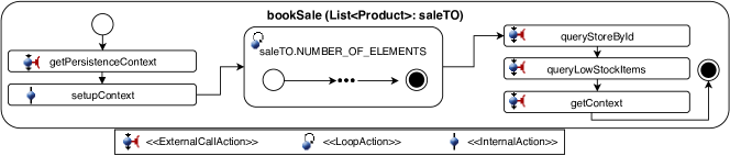
Figure 3: SEFF of CoCoME’s ”bookSale” service

IX Evaluation

This section introduces the evaluation goals, setup, environment and the results of the evaluation:

IX-A Evaluation Goals

The goal is to evaluate the following three aspects of the approach and answer the Evaluation-Questions (EQs):

• Accuracy of the incremental calibration:
  EQ1.1: How accurate are the incremental calibrated PMs?
  EQ1.2: Is the accuracy of the incremental calibrated PM stable over the incremental evolution?

• Accuracy of the parametric dependencies:
  EQ2: Does the estimation of parametric dependencies improve the accuracy of PMs?

• Performance of the calibration pipeline:
  EQ3: How long does the pipeline need to update PMs?

• Monitoring overhead:
  EQ4.1: How much is the required monitoring overhead?
  EQ4.2: How much can the adaptive instrumentation reduce the monitoring overhead?

IX-B Experiment Setup

The evaluation is structured as follows:
1. We monitor the application over a defined period of time (e.g., 60 minutes) and perform a load test at the same time to artificially simulate user interactions.
2. We run the monitoring in combination with the load test two times. First, we apply a fine-grained monitoring, pass the results to the calibration pipeline for adjusting the architecture model (training set). Second, we only observe service calls (coarse-grained monitoring). These data are used to estimate the accuracy of the calibrated model (validation set). This procedure prevents the monitoring overhead from falsifying the evaluation results. We also record the execution times (overhead) of the pipeline parts.3. We adjust the usage model according to the validation set and perform a fixed number of simulations of the updated architecture model (100 repetitions). Repetitions are necessary, as the simulation samples from stochastic distributions may not be representative. Afterward, we compare the results of the simulations with the validation set. Both are distributions, therefore we use the Kolmogorov-Smirnov-Test (KS-Test) [14], the Wasserstein metric [35], and conventional statistical measures to determine the similarity. The lower the KS-Test value, the higher is the accuracy of the updated architecture model. In order to limit the dependence on a single metric, we also included the Wasserstein distance to confirm the results. The Wasserstein metric is distance measure that quantifies the effort needed to transfer one distribution into the other. If we want to compare the accuracy of two simulation distributions (using real monitoring as reference), this metric is well suited, but reports absolute numbers that are difficult to interpret. We therefore combined both metrics in our analysis.

IX-C Evaluation Environments

We evaluated our approach using two case studies: Common Component Modeling Example (CoCoME) [22] and TeaStore [25]. CoCoME is a trading system which is designed for the use in supermarkets. It supports several processes like scanning products at a cash desk or processing sales using a credit card. We used a cloud-based implementation of CoCoME where the enterprise server and the database run in the cloud.

Additionally, we evaluated our approach using the aforementioned running example of the TeaStore case study (cf. Section III). Compared to the original, we modified the application so that the ”train” service is executed when a user places an order. This causes the number of users to have a direct impact on the service response times.

Because CoCoME and TeaStore are not implemented using the Vitruvius platform, we instrument the changed parts of the source code manually. In future work, we will use approaches for importing existing source code into Vitruvius [34], which allows the automatic adaptive instrumentation.

IX-D Evaluation of the Incremental Calibration

This section evaluates the accuracy of our calibration for the following incremental evolution scenarios.

IX-D1 BookSale Calibration

The “bookSale” service of CoCoMe case study is responsible for processing a sale after a user submitted his payment. As input, this service receives a list of the purchased products including all information related to the purchase. The service consists of several internal and external actions and two loops. Figure 3 visualizes the structure of the calibrated ”bookSale” service of CoCoME. For reasons of simplification, we focused on the structure and omitted certain details. In this evaluation scenario, we supposed that the “bookSale” service is newly added. According to our assumption, we instrumented this service and all services that are subsequently called by it. We performed a load test which simulates user purchases. We used the resulting monitoring data to calibrate our architecture model.

Results

Table I shows the quartiles for both the monitoring and the simulation results for a single example execution. Besides, a KS test value of 0.1321 and a Wasserstein distance of 13.7726 were obtained by comparing the monitoring and the simulation distributions. It is well visible that these distributions are very close to each for the first, second and third quartile. The discrepancy in the minimum and maximum values of the distributions arises because we limited the time spent for simulation. The KS tests average over all 100 simulation runs is approximately 0.1467 (min 0.1248, max 0.1774). These results confirm the PM accuracy (EQ1.1).

TABLE I: Quartiles for the probability distributions of a single simulation and the monitoring for the ”bookSale” service

Distribution	Min	Q1	Q2	Q3	Max	Avg
Monitoring	31ms	101ms	130ms	187ms	461ms	143ms
Simulation	56ms	95ms	124ms	163ms	338ms	133ms

IX-D2 Train Calibration

Similar to ”BookSale” evaluation scenario, we assumed that ’train’ service (cf. Section III) was newly added. Therefore, we instrumented and monitored the statements of all SEFF elements shown in Fig. 1 in two cases: (1) for the first implementation of ’train’ and (2) after adding an enumeration parameter that refers to the used implementation of ’train’ to represent the four implementations in one SEFF (cf. Sec. IX-E). Then we calibrated the SEFFs of these two cases. Due to lack of space we show only the accuracy results of the second case in (Table III, 2 column).

IX-D3 TrainForRecommender Calibration

To evaluate that the accuracy of PM is stable (EQ1.2), we simulated an evolution scenario that assumes that the developers change the implementation of the ’train’ service to examine the four implementation alternatives (cf. Section III) in four subsequent source code commits $c1$, …, $c4$. According to our assumption, except of the ”trainForRecommender” internal action, the behavior of ’train’ (Figure 1) stays the same. To evaluate this scenario, we instrumented only the ”trainForRecommender” internal action for the first implementation of ’train’ ($c1$). We performed 15 minutes of fine-granular monitoring and used the resulting data to calibrate the model. Next, we monitored the ’train’ service for another 15 minutes of coarse granular. The coarse granular monitoring data was used as reference for the estimation of the accuracy of PM. In the next step, we instrumented the ”trainForRecommender” internal action for the second implementation of ’train’ ($c2$) and performed a fine granular and a coarse granular monitoring for 15 minutes each. We repeated the same procedure for commits $c3$ and $c4$.

To simulate additional commits, we changed the train implementation by randomly replacing the strategy with another one. We repeated this procedure six more times to simulate six additional iterations and calculate the accuracy of the calibrated model for each iteration. In addition, the database filled up over time, which leads to increasing response times, increasing the difficulty for the calibration process.

Results

TABLE II: Aggregated metrics of the evolution scenario

Metric	Min	Median	Max	Avg	St.Dev
KS Test	0.222	0.257	0.317	0.256	0.028
WS Distance	24.56	33.74	38.96	33.76	4.01

Table II lists the aggregated results. The values are slightly higher than without applying changes to the application. However, it can be seen that the accuracy of the models is almost constant throughout the evolutionary steps. From this, we conclude that the automated calibration is able to handle changes of the observed services.

IX-E Evaluation of the Estimation of Parametric Dependencies

This scenario evaluates the recognition of the parametric dependencies and compares the accuracy of the AbPP using the parameterized model (i.e., calibrated with our approach) with the non-parameterized model (i.e., calibrated ignoring parametric dependencies). For this goal, we extended the SEFF shown in Figure 1 and added an enumeration input parameter that refers to the recommender type and determines which implementation is used within the ”trainForRecommender” internal action. This allowed us to represent all different implementations in one SEFF. This means the RD of ”trainForRecommender” can be related to the recommender type. Then, we calibrated the SEFF and predicted the performance for increasing the load from 20 to 40 concurrent users. First, we monitored the service fine granular (F1) and subsequently coarse granular (C1) by applying the load of 20 users. We only used the resulting monitoring data (F1) to calibrate a parameterized model using our approach and the non-parameterized model using the distributions of the observed values. Then, we compared the simulation results of both models with the monitoring data (C1). Then, we performed AbPP for the higher load (40 users). As baseline, we measured the performance using coarse granular monitoring and applying the load of 40 users (C2). Finally, we compared the AbPP results of both models with the monitoring data (C2).

Results

The results confirmed that our calibration was able to detect the parametric dependencies. Hence, the RD of trainForRecommender is related to the type of recommendation implementation and the number of elements.

Table III shows the comparison of the KS tests and the Wasserstein distances between the parameterized and the non-parameterized model. It can be seen that both models are very accurate for the standard load of 20 users. However, the non-parametric model loses significantly more accuracy than the parameterized model, when the load changes to 40 users. This confirms that the estimation of the parametric dependencies improves the accuracy of PMs (EQ1.1, EQ2).

TABLE III: Comparison between the accuracy of the parameterized (PM) and the non-parameterized (NPM) model.

Metric	PM (20 Users)	NPM (20 Users)	PM (40 Users)	NPM (40 Users)
KS Q1	0.1024	0.1023	0.1378	0.2352
KS Avg.	0.1267	0.1239	0.1609	0.2575
KS Q3	0.1431	0.1441	0.1810	0.2834
WS Q1	15.4911	11.2484	33.0235	43.5959
WS Avg.	19.1764	16.2669	39.6138	51.3531
WS Q3	22.2654	18.2179	46.8370	59.9197

IX-F Evaluation of the MbDevOps Pipeline

This section evaluates the performance of the implemented part of MbDevOps Pipeline (monitoring, incremental calibration and self-validation) and answers EQ3. For that, we computed how long the individual pipeline parts took to complete. We used the three evolution scenarios described in Section IX-D. The results are shown in Table IV.

TABLE IV: Execution times of the pipeline parts

Measure	bookSale	train	trainForRecommender
Record Count	220706	294237	27085
Load Records	4.664s	5.142s	0.774s
PM Calibration	9.168s	4.996s	0.789s
UM Adjustment	2.365s	0.194s	0.165s
Self-Validation	1.729s	1.440s	1.327s
Total	17.926s	11.772s	3.055s

We can see that the required time strongly depends on the number of monitoring records and the complexity of the observed service. Except for the self-validation, the execution time of all parts of the pipeline depends on the number of records (see Table V). In all considered cases, the execution of the whole pipeline took less than 20 seconds.

We observe that adaptive monitoring limits the number of monitoring records. Accordingly, the second iteration of TeaStore monitoring produces far fewer records, which results in significantly lower execution times. To gain detailed insights about the performance of the pipeline, we also examined the behavior for an increasing number of monitoring records. For this purpose, we generated monitoring data using CoCoME and the load test that we also used before. Thereafter, we executed the pipeline several times, with an increasing number of monitoring records as input. The results in Table V showed that the execution time of the pipeline scales linearly with the number of monitoring records in this case.

TABLE V: Detailed performance information for an increasing number of monitoring records

Number of records	Loading Records	PM Calibration	UM Adjustment	Sum
100000	1.570s	6.899s	1.158s	9.627s
200000	3.018s	7.229s	1.860s	12.107s
500000	6.290s	7.899s	1.802s	15.991s
700000	9.972s	8.194s	1.942s	20.108s
1000000	14.780s	9.160s	1.917s	25.857s

IX-G Evaluation of Monitoring Overhead

To answer the EQ4.1 and EQ4.2, we measured the overhead caused by the monitoring for the incremental calibration scenarios in Section IX-D.

The average monitoring overhead for bookSale was 1.31ms (fine-grained), 252$\mu$s (coarse-grained) and for train 1.81ms (fine-grained), 88$\mu$s (coarse-grained). We note that the coarse-grained monitoring has a negligible influence. The fine-grained monitoring overhead scales with the complexity of the service. In our case, the overhead of around 1ms had no drastic impact on the performance, since the execution times of the services are significantly higher.

The evolution of TrainForRecommender calibration scenario (cf. Section IX-D3) shows very well that the adaptive monitoring helps to significantly reduce the monitoring overhead. Comparing to train (cf. Section IX-D2) where all SEFF elements are instrumented, we saved at least 75% of the monitoring overhead by instrumenting only the changed internal action. This is reflected in the calibration times, which are considerably lower compared to the first iteration (see Table IV) (EQ4.2). In general, there is a trade off between the monitoring overhead and the accuracy of the model. However, our approach tries to balance them by using the incremental calibration in combination with the adaptive monitoring in order to minimize calibration time and monitoring overhead.

X Related Work

A number of approaches for constructing the architectural model based on static (e.g., [2]), dynamic, or hybrid analysis exist. Walter et al. [48] propose a tool to extract an architectural PM as well as performance annotation based on analysing monitoring traces. Similarly, other works [3, 44, 10] extract PM based on dynamic analysis. Krogmann et al. [30, 29] extract parametrized PCM based on hybrid analysis. Langhammer et al. introduce two reverse engineering tools [31, P. 140] [33] that extract the behavior of the underlying source code based on hybrid analysis.

The above-mentioned approaches do not support the iterative extraction of the architectural PMs or the incremental calibration. If they were used in an iterative development, they would re-extract and recalibrate the whole models after each iteration. This would cause a high monitoring overhead. Moreover, this process ignores the potential manual modifications of the extracted PM that may be formerly applied.

In addition to the work of Krogmann et al. [30, 29], the works of Ackermann et al. [1] and Curtois et al. [13] also consider the characterization of parametric dependencies in performance models, while Grohmann et al. [15] focus on the identification of those from monitoring data. However, our work considers the parametric dependencies during the incremental calibration of the architectural PMs.

Model extraction approaches derive the resource demands either based on coarse-grained monitoring data [45, 46] or fine-grained data [5, 50]. The latter approaches give a higher accuracy by estimating PMPs but have a downside effect because of the overhead of instrumentation and the monitoring. Our approach reduces the overhead by the automatic adaptive instrumentation and monitoring.

Spinner et al. [47] propose an agent-based approach to updated architectural performance models. In contrast to our work, they focus on model updates at run-time.

Declarative Performance Engineering (DPE) [49] technically enables to answer concerns based on measurement-based performance evaluation and model-based performance predictions. However, existing solutions do not provide a technical integration into the build pipeline. Also, DPE does not answer how to keep PMs updated.

XI Conclusion and future works

Applying AbPP in the agile and DevOps process promises to detect performance problems by simulation instead of the execution in a production environment. We presented the continuous integration of the architectural performance model in the development process based on the static and dynamic analysis of the changed code. Our approach keeps the PM continuously up-to-date. We also presented the MbDevOps pipeline which automates the incremental calibration process.

Our calibration estimates the parametrized PMPs incrementally and uses a novel incremental resource demand estimation based on adaptive monitoring. Moreover, our calibration updates both the usage and deployment models to support model-based run-time performance management like auto-scaling.

We tested the functionality using two case studies. The evaluation showed the ability to calibrate the PM incrementally. We evaluated the accuracy of our calibration by comparing the simulation results with the monitoring data. In these case studies, the incrementally calibrated models and their parametric dependencies were accurate and the used adaptive monitoring significantly reduced the monitoring overhead and the calibration effort.

In this work, we have automated only the part of the proposed MbDevOps pipeline that is responsible for testing, incremental calibration and self-validation.

In future work, we aim to automate the whole pipeline to integrate the continuous integration (CI) process with Vitruvius. Moreover, we will extend the available approaches to integrate existing source code and models into Vitruvius platform [34, 38].

Besides, we will extend our parametrized calibration to test for more complex dependencies of external call parameters. It is also planned to extend the monitoring records to update the system model (composition of the components) automatically.

References

- [1] Vanessa Ackermann, Johannes Grohmann, Simon Eismann and Samuel Kounev “Black-box Learning of Parametric Dependencies for Performance Models” In Proceedings of 13th Workshop on Models@run.time (MRT), co-located with MODELS 2018, CEUR Workshop Proceedings, 2018
- [2] Becker al. “Reverse engineering component models for quality predictions” In 2010 14th European Conference on Software Maintenance and Reengineering, 2010 IEEE
- [3] Brunnert al. “Automatic Performance Model Generation for Java Enterprise Edition (EE) Applications” In Computer Performance Engineering, 2013
- [4] C. Woodside al. “The Future of Software Performance Engineering” In Future of Software Engineering (FOSE ’07), 2007, pp. 171–187
- [5] Fabian Brosig al. “Automated Extraction of Palladio Component Models from Running Enterprise Java Applications” In Proceedings of the 1st Int. Workshop on Run-time models for Self-managing systems and applications. In conjunction with the Fourth Int. Conference on Performance Evaluation Methodologies and Tools (VALUETOOLS 2009), 2009
- [6] Reiner Jung al. “Model-driven instrumentation with Kieker and Palladio to forecast dynamic applications” In Symposium on Software Performance CEUR, 2013 URL: http://ceur-ws.org/Vol-1083/paper11.pdf
- [7] S. Balsamo, A. Di Marco, P. Inverardi and M. Simeoni “Model-based performance prediction in software development: a survey” In IEEE Transactions on Software Engineering 30.5, 2004, pp. 295–310 DOI: 10.1109//TSE.2004.9
- [8] Steffen Becker, Heiko Koziolek and Ralf Reussner “The Palladio component model for model-driven performance prediction” In Journal of Systems and Software 82 Elsevier Science Inc., 2009, pp. 3–22 DOI: 10.1016/j.jss.2008.03.066
- [9] Cor-Paul Bezemer et al. “How is Performance Addressed in DevOps?” In Proceedings of the 2019 ACM/SPEC Int. Conference on Performance Engineering, 2019, pp. 45–50
- [10] Fabian Brosig, Nikolaus Huber and Samuel Kounev “Automated Extraction of Architecture-Level Performance Models of Distributed Component-Based Systems” In 26th IEEE/ACM Int. Conference On Automated Software Engineering (ASE 2011), 2011
- [11] Andreas Brunnert et al. “Performance-oriented DevOps: A Research Agenda”, 2015 URL: http://arxiv.org/abs/1508.04752
- [12] Erik Burger “Flexible Views for View-based Model-driven Development”, The Karlsruhe Series on Software Design and Quality Karlsruhe, Germany: KIT Scientific Publishing, 2014 DOI: 10.5445/KSP/1000043437
- [13] Marc Courtois and Murray Woodside “Using Regression Splines for Software Performance Analysis” In Proceedings of the 2nd Int. Workshop on Software and Performance, 2000
- [14] Yadolah Dodge “Kolmogorov–Smirnov Test” In The Concise Encyclopedia of Statistics New York, NY: Springer New York, 2008, pp. 283–287 DOI: 10.1007/978-0-387-32833-1˙214
- [15] Johannes Grohmann et al. “Detecting Parametric Dependencies for Performance Models Using Feature Selection Techniques” In Proceedings of the 27th IEEE Int. Symposium on the Modelling, Analysis, and Simulation of Computer and Telecommunication Systems, MASCOTS ’19, 2019
- [16] M. Hall et al. “The WEKA data mining software” In ACM SIGKDD Explorations Newsletter 11.1 Association for Computing Machinery (ACM), 2009, pp. 10
- [17] Christoph Heger, André Hoorn, Mario Mann and Dušan Okanović “Application Performance Management: State of the Art and Challenges for the Future” In Proceedings of the 8th ACM/SPEC on Intl. Conference on Performance Engineering, ICPE ’17 L’Aquila, Italy: ACM, 2017, pp. 429–432 DOI: 10.1145/3030207.3053674
- [18] Florian Heidenreich, Jendrik Johannes, Mirko Seifert and Christian Wende “Closing the Gap between Modelling and Java” In Software Language Engineering 5969, Lecture Notes in Computer Science Springer Berlin Heidelberg, 2010, pp. 374–383 DOI: 10.1007/978-3-642-12107-4˙25
- [19] Robert Heinrich “Architectural Run-time Models for Performance and Privacy Analysis in Dynamic Cloud Applications” In ACM SIGMETRICS Performance Evaluation Review 43.4 New York, NY, USA: ACM, 2016, pp. 13–22 DOI: 10.1145/2897356.2897359
- [20] Robert Heinrich et al. “Integrating Run-time Observations and Design Component Models for Cloud System Analysis” In Proceedings of the 9th Workshop on Models@run.time co-located with 17th Int. Conference on Model Driven Engineering Languages and Systems (MODELS 2014), Valencia, Spain, September 30, 2014., 2014, pp. 41–46 URL: http://ceur-ws.org/Vol-1270/mrt14_submission_8.pdf
- [21] Robert Heinrich et al. “Software Architecture for Big Data and the Cloud” to appear Elsevier, 2017
- [22] R. Heinrich et al. “The CoCoME Platform: A Research Note on Empirical Studies in Information System Evolution” In Int. Journal of Software Engineering and Knowledge Engineering 25.09&10, 2015, pp. 1715–1720 DOI: 10.1142/S0218194015710059
- [23] André Hoorn, Jan Waller and Wilhelm Hasselbring “Kieker: A Framework for Application Performance Monitoring and Dynamic Software Analysis” In Proceedings of the 3rd ACM/SPEC Int. Conference on Performance Engineering, ICPE ’12 ACM, 2012, pp. 247–248
- [24] Jan-Philipp Jägers “Iterative Performance Model Parameter Estimation Considering Parametric Dependencies”, 2019
- [25] Jóakim Kistowski et al. “TeaStore: A Micro-Service Reference Application for Benchmarking, Modeling and Resource Management Research” In 2018 IEEE 26th Int. Symposium on Modeling, Analysis, and Simulation of Computer and Telecommunication Systems (MASCOTS), 2018, pp. 223–236 IEEE
- [26] Heiko Koziolek “Modeling Quality” In Modeling and simulating software architectures: the Palladio approach Cambridge, Massachusetts: MIT Press, 2016
- [27] Max E. Kramer, Erik Burger and Michael Langhammer “View-Centric Engineering with Synchronized Heterogeneous Models” In Proceedings of the 1st Workshop on View-Based, Aspect-Oriented and Orthographic Software Modelling, VAO ’13 Montpellier, France: ACM, 2013, pp. 5:1–5:6 DOI: 10.1145/2489861.2489864
- [28] Max E. Kramer et al. “Extending the Palladio Component Model using Profiles and Stereotypes” In Palladio Days 2012 Proceedings (appeared as technical report), Karlsruhe Reports in Informatics ; 2012,21 Karlsruhe: KIT, Faculty of Informatics, 2012, pp. 7–15 URL: http://nbn-resolving.org/urn:nbn:de:swb:90-308043
- [29] Klaus Krogmann “Reconstruction of Software Component Architectures and Behaviour Models using Static and Dynamic Analysis” 4, The Karlsruhe Series on Software Design and Quality KIT Scientific Publishing, 2012
- [30] Klaus Krogmann, Michael Kuperberg and Ralf Reussner “Using Genetic Search for Reverse Engineering of Parametric Behaviour Models for Performance Prediction” In IEEE Transactions on Software Engineering IEEE, 2010
- [31] Michael Langhammer “Automated Coevolution of Source Code and Software Architecture Models”, 2017 DOI: 10.5445/IR/1000069366
- [32] Michael Langhammer and Klaus Krogmann “A Co-evolution Approach for Source Code and Component-based Architecture Models” In 17. Workshop Software-Reengineering und-Evolution 4, 2015 URL: http://fg-sre.gi.de/fileadmin/gliederungen/fg-sre/wsre2015/WSRE2015-Proceeedings-preliminary.pdf#page=40
- [33] Michael Langhammer, Arman Shahbazian, Nenad Medvidovic and Ralf H Reussner “Automated extraction of rich software models from limited system information” In 2016 13th Working IEEE/IFIP Conference on Software Architecture (WICSA), 2016 IEEE
- [34] Sven Leonhardt, Benjamin Hettwer, Johannes Hoor and Michael Langhammer “Integration of Existing Software Artifacts into a View- and Change-Driven Development Approach” In Proceedings of the 2015 Joint MORSE/VAO Workshop on Model-Driven Robot Software Engineering and View-based Software-Engineering, MORSE/VAO ’15 ACM, 2015, pp. 17–24
- [35] Szymon Majewski et al. “The Wasserstein Distance as a Dissimilarity Measure for Mass Spectra with Application to Spectral Deconvolution” In 18th Int. Workshop on Algorithms in Bioinformatics (WABI 2018) 113, Leibniz Int. Proceedings in Informatics (LIPIcs) Dagstuhl, Germany: Schloss Dagstuhl–Leibniz-Zentrum fuer Informatik, 2018, pp. 25:1–25:21
- [36] Anne Martens, Heiko Koziolek, Lutz Prechelt and Ralf Reussner “From monolithic to component-based performance evaluation of software architectures” In Empirical Software Engineering 16.5 Springer Netherlands, 2011, pp. 587–622 DOI: 10.1007/s10664-010-9142-8
- [37] Manar Mazkatli and Anne Koziolek “Continuous Integration of Performance Model” In Companion of the 2018 ACM/SPEC Int. Conference on Performance Engineering, ICPE ’18 Berlin, Germany: ACM, 2018 DOI: 10.1145/3185768.3186285
- [38] Manar Mazkatli, Erik Burger, Jochen Quante and Anne Koziolek “Integrating semantically-related Legacy Models in Vitruvius” In Proceedings of Modelling in Software Engineering co-located with the 40th International Conference on Software Engineering, 2018 DOI: https://doi.org/10.1145/3193954.3193961
- [39] Daniel A Menasce, Virgilio AF Almeida, Lawrence W Dowdy and Larry Dowdy “Performance by design: computer capacity planning by example” Prentice Hall Professional, 2004
- [40] Mathias Meyer “Continuous integration and its tools” In IEEE software 31.3 IEEE, 2014, pp. 14–16
- [41] J. Quinlan “C4.5: Programs for Machine Learning” San Francisco, CA, USA: Morgan Kaufmann Publishers Inc., 1993
- [42] Ralf H. Reussner et al. “Modeling and Simulating Software Architectures – The Palladio Approach” Cambridge, MA: MIT Press, 2016 URL: http://mitpress.mit.edu/books/modeling-and-simulating-software-architectures
- [43] Connie U. Smith and Lloyd G. Williams “Performance Solutions: A Practical Guide to Creating Responsive, Scalable Software” Redwood City, CA, USA: Addison Wesley Longman Publishing Co., Inc., 2003
- [44] Simon Spinner, Jürgen Walter and Samuel Kounev “A Reference Architecture for Online Performance Model Extraction in Virtualized Environments” In Companion Publication for ACM/SPEC on Int. Conference on Performance Engineering, 2016, pp. 57–62 ACM
- [45] Simon Spinner, Giuliano Casale, Fabian Brosig and Samuel Kounev “Evaluating approaches to resource demand estimation” In Performance Evaluation 92 Elsevier, 2015
- [46] Simon Spinner, Giuliano Casale, Xiaoyun Zhu and Samuel Kounev “LibReDE: A Library for Resource Demand Estimation” In Proceedings of the 5th ACM/SPEC Int. Conference on Performance Engineering, ICPE ’14 ACM, 2014
- [47] Simon Spinner, Johannes Grohmann, Simon Eismann and Samuel Kounev “Online model learning for self-aware computing infrastructures” In Journal of Systems and Software 147, 2019, pp. 1–16
- [48] Jürgen Walter, Christian Stier, Heiko Koziolek and Samuel Kounev “An Expandable Extraction Framework for Architectural Performance Models” In Proceedings of the 8th ACM/SPEC on Int. Conference on Performance Engineering Companion, ICPE ’17 Companion L’Aquila, Italy: ACM, 2017, pp. 165–170 DOI: 10.1145/3053600.3053634
- [49] Jürgen Walter et al. “Tools for Declarative Performance Engineering” In Companion of the 2018 ACM/SPEC Int. Conference on Performance Engineering, ICPE ’18 Berlin, Germany: ACM, 2018, pp. 53–56 DOI: 10.1145/3185768.3185777
- [50] Felix Willnecker et al. “Comparing the accuracy of resource demand measurement and estimation techniques” In European Workshop on Performance Engineering, 2015 Springer