A time-domain preconditioner for the Helmholtz equation

Abstract.

Time-harmonic solutions to the wave equation can be computed in the frequency or in the time domain. In the frequency domain, one solves a discretized Helmholtz equation, while in the time domain, the periodic solutions to a discretized wave equation are sought, e.g. by simulating for a long time with a time-harmonic forcing term. Disadvantages of the time-domain method are that the solutions are affected by temporal discretization errors and that the spatial discretization cannot be freely chosen, since it is inherited from the time-domain scheme. In this work we address these issues. Given an indefinite linear system satisfying certain properties, a matrix recurrence relation is constructed, such that in the limit the exact discrete solution is obtained. By iterating a large, finite number of times, an approximate solution is obtained, similarly as in a time-domain method for the Helmholtz equation. To improve the convergence, the process is used as a preconditioner for GMRES, and the time-harmonic forcing term is multiplied by a smooth window function. The construction is applied to a compact-stencil finite-difference discretization of the Helmholtz equation, for which previously no time-domain solver was available. Advantages of the resulting solver are the relative simplicity, small memory requirement and reasonable computation times.

1. Introduction

Time-harmonic solutions to the wave equation can be computed in the frequency or in the time domain. In the frequency domain, a discrete version of the Helmholtz equation is solved. In the time domain, the periodic solutions to a discrete wave equation with time-harmonic forcing term are sought. Frequency domain methods involve less degrees of freedom. However, the indefinite linear systems resulting from discretizing the Helmholtz equation are often difficult to solve. Time-domain methods can be attractive because they require relatively little memory and are easy to implement if a time-domain solver is available. The introduction of [1] contains a recent overview of time-harmonic wave equation solvers.

Time-domain methods are based on the correspondence between Helmholtz and wave equations. In this paper we will use as example the damped wave equation

(1) $$\frac{1}{c^{2}}\frac{\partial^{2}u}{\partial t^{2}}+R\frac{\partial u}{\partial t}-\Delta u=f,$$

where $u=u(t,x)$ is the wave field, $f=f(t,x)$ is the forcing term, $\Delta$ is the Laplacian, $c(x)$ is the spatially dependent wavespeed, $R$ is a spatially dependent damping coefficient, and $x$ is in some domain $\Omega$ with Dirichlet and/or Neumann boundary conditions. Let $u(x,t),f(x,t)$ and $U(x),F(x)$ be related by

(2) $$u(x,t)=e^{i\omega t}U(x),\qquad\text{ and }f(x,t)=e^{i\omega t}F(x).$$

Then $u$ satisfies a wave equation with forcing term $f$ if and only if $U$ satisfies the following Helmholtz equation with forcing term $F$

(3) $$-\Delta U-\frac{\omega^{2}}{c^{2}}U+i\omega RU=F.$$

This equation is supplemented with Dirichlet and/or Neumann boundary conditions that carry over from those for (1).

We briefly review some time-domain approaches. The most basic time-domain method is derived from the limiting-amplitude principle. This principle states that solutions $u(x,t)$ to (1) with zero initial conditions and forcing term

(4) $$f(x,t)=e^{i\omega t}F(x)$$

satisfy

(5) $$u(x,t)=e^{i\omega t}U(x)+O(1),\qquad t\to\infty$$

under certain conditions on the problem, see [4] and references therein. Thus, if $u(x,t)$ is a (numerical) solution to this initial boundary-value problem, and $T$ is some large time, measured in periods, then an approximate solution to the Helmholtz equation is given by

(6) $$e^{-i2\pi T}u(x,2\pi\omega^{-1}T).$$

We will call this the limiting-amplitude approximate solution for time $T$. A more advanced method is the exact controllability method [5]. In this method the periodicity of the solutions is enforced using optimization. The starting value for the optimization procedure is typically some partially converged limiting-amplitude solution. Recently more insights in and some improvements to this method were obtained [11], and its parallel implementation was studied [10]. In [1] an optimization approach called WaveHoltz was introduced. This method again uses a form of optimization but with a different optimization functional.

An important feature of the methods just described is that they approximate periodic solutions of a given discrete wave equation. This has two consequences that are in general not desirable. First, the results will be negatively affected by both spatial and temporal discretization errors, while solutions to discrete Helmholtz equations only have spatial discretization errors. Secondly, the method is limited to situations in which a time-domain scheme is available, and not (directly) applicable if one only has a discretization of (3) available, or perhaps only a linear system with similar properties.

In this paper, we will address both of these shortcomings by developing a new time-domain solver for discrete Helmholtz equations. The method takes as a starting point a linear system

(7) $$HU=F,$$

where $H$ is a complex $N\times N$ matrix, such that

(8) $$\text{$\operatorname{Re}H$ is symmetric},$$

and

(9) $$\text{$\operatorname{Im}H$ is symmetric positive semidefinite}.$$

In equation (7) $F$ is a vector in ${\mathbb{C}}^{N}$ and $U$ is the unknown, also in ${\mathbb{C}}^{N}$. The applications we have in mind are discretized Helmholtz equations and other time-harmonic wave equations. For a certain finite difference discretization of the Helmholtz equation the method will be worked out in detail and numerical results will be given. We next describe the steps involved in the construction of the new time-domain solver.

First an $N\times N$ system of second order ODE’s

(10) $$\frac{\partial u^{2}}{\partial t^{2}}+Au+B\frac{\partial u}{\partial t}=f$$

and a frequency parameter $\omega$ are constructed. We will look for time-harmonic solutions with frequency $\omega$ of the system (10). Note that $\omega$ is in general not the physical frequency parameter used to derive (7). It is a computational parameter, chosen together with the matrices $A$ and $B$, and it depends on $H$ in a way to be specified. Time-harmonic functions $u=e^{i\omega t}U$ and $f=e^{i\omega t}F$, with $U,F\in{\mathbb{C}}^{N}$, satisfy (10) if and only if

(11) $$(-\omega^{2}I+i\omega B+A)U=F.$$

Therefore we will choose $A,B$ and $\omega$ such that

(12) $$H=-\omega^{2}I+i\omega B+A.$$

The system (10) plays the role of a semi-discrete wave equation.

Secondly, this system is time-discretized. This is done in such a way that time-harmonic solutions of the discrete-time system are exactly those of the continuous-time system. I.e. if $u_{n},f_{n}$ are related to $U,F$ by $u_{n}=e^{i\omega n\Delta t}U$ and $f_{n}=e^{i\omega n\Delta t}F$ then $u_{n},f_{n}$ are solutions to the discrete-time system if and only if $U,F$ satisfy (11). For this purpose we present two modified leapfrog methods. This is related to ideas from the papers [12, 22], see also the optimized time-stepping method in [3].

Having a time-discretization of (10) at hand, the third step is to define a map from a right-hand side $F$ in (7) to an approximation for the solution $U$. For this we follow the idea of equation (6) with one modification, which is the inclusion of a smooth window function in the time-harmonic forcing term.

It is known that the convergence of limiting-amplitude approximate solutions can be slow in some cases, e.g. in case of resonant wave cavities. Therefore we will not use the approximate solution operator directly, but use it as a preconditioner in an iterative solution method such as GMRES or BiCGSTAB (Krylov accelleration). This is the fourth and last step of our construction. The new approximate solution operator will be called a time-domain preconditioner. The term time-domain preconditioner was used before in [26]. In that work a related problem was solved, but the resulting method was substantially different. The above distinction between frequency- and time-domain methods appears no longer satisfactory for this method: It is based on time-domain methodology, but solves a frequency-domain discrete wave equation.

Conditions for stability of the new time-discretization and the convergence for large $T$ of the approximate solutions to the exact solution of (7) will be established theoretically, including estimates for the convergence if $\operatorname{Im}H=0$. Numerical examples confirm the converge of the approximate solutions and show the usefulness of Krylov accelleration in cases where a resonant low-velocity zone is present. Results depend weakly on the large time parameter $T$ used in the preconditioner, and a parameter for the window function, i.e. there is a large set of suitable parameter choices.

A few situations that do not fit in the classical time-domain setting, but can be handled with the new solver are as follows. First one can use it with discretizations that have been designed specifically for the Helmholtz equation. For example finite-difference discretizations that minimize dispersion errors such as those from [2] for the 2-D case and [18, 21, 24] for the 3-D case. Our examples are about this application. One can also imagine situations where the physical time-domain model is complicated to simulate, but reduces to a relatively simple Helmholtz equation in the frequency domain. A third use case is in the context of a multigrid method. In multigrid methods the coarsest level system still has to be solved by another (non-multigrid) method. It is based on the linear system one started with and on the choice of multigrid method. In Helmholtz equations the convergence can be very sensititve to the choice of the coarse level system and it is recommended to use certain prescribed discretizations [20, 18].

However, the usefulness of the method is not restricted to these cases, and some of the ideas could also be incorporated into other time-domain methods.

The contents of the remainder of the paper is as follows. In section 2, the construction of the new solver is described. In section 3 examples of this construction are given in case $H$ results from certain finite-difference discretizations. Section 4 contains the theoretical results. After that, section 5 contains the numerical examples. So far it was assumed that $\operatorname{Im}H$ is diagonal, in order for the time stepping method to be explicit. Section 6 describes a variant of the method that involves an explicit time stepping method even if $\operatorname{Im}H$ is non-diagonal. We conclude the main text with a discussion section. Appendices contain some remarks on the compact-stencil finite-difference discretization described in section 3 and the derivation of a Fourier transform used in section 4.

2. Method

In this section we describe in detail the construction of a time-domain preconditioner for a matrix $H$ satisfying (8) and (9). We recall from the introduction that there are three main steps: (i) the definition of a suitable second order system of ODE’s of the form (10); (ii) the definition of a suitable time-integration method for this system of ODE’s; (iii) the definition of a linear map that produces approximate solutions based on the limiting-amplitude principle. Step (ii), the time-integration method, will be discussed first, since the properties of the time-integration method affect the choice of the system of ODE’s (10). Then steps (i) and (iii) and the application of the method as a preconditioner are discussed.

2.1. Frequency-adapted time discretizations of (10)

The leapfrog or basic Verlet method is a standard method to integrate equations of the form (10) in case that $B=0$. It is obtained, basically, by discretizing the second order time derivative using standard second order finite differences. To allow for nonzero $B$, the damping term has to be discretized as well. A standard way to do this is with central differences [6, 17, 16]. This yields the equation

(13) $$\frac{1}{\Delta t^{2}}\left(u_{n+1}-2u_{n}+u_{n-1}\right)+\frac{1}{2\Delta t}B\left(u_{n+1}-u_{n-1}\right)+Au_{n}=f_{n},$$

from which $u_{n+1}$ can be solved. Note that $u_{n}$ denotes the discrete approximation to $u(n\Delta t)$, and that $u(t)\in{\mathbb{C}}^{N}$.

This leads to an explicit method only if $B$ is diagonal. In section 6 we will discuss a variant that results in an explicit method in case $B$ is non-diagonal.

We will formally define the time-integrator resulting from (13).

Definition 1.

Let

(14) $$K={} \Delta t^{2}A\qquad{} L={} \Delta tB\qquad{} g_{n}=\Delta t^{2}f_{n}.$$

Central differences damped leapfrog will be defined as the time integrator given by

(15) $$u_{n+1}=I_{\rm cd}(u_{n},u_{n-1},f_{n}):=\left(I+\tfrac{1}{2}L\right)^{-1}\left((2-K)u_{n}-(I-\tfrac{1}{2}L)u_{n-1}+g_{n}\right).$$

The stability of these methods is discussed in section 4. According to Theorem 1, $I_{\rm cd}$ is stable if

(16) $$\text{$K$ and $L$ are positive semidefinite},$$

and

(17) $$\text{$4I-K$ is positive definite}.$$

The latter condition leads to a CFL bound, that will be discussed below.

As mentioned in the introduction, we look for discretizations such that the time-harmonic solutions of frequency $\omega$ of the discrete-time system are exactly those of the continuous time system (10). Due to discretization errors this is not the case for $I_{\rm cd}$. In the next proposition we will show that the time-harmonic solutions to (10) satisfy a recursion of the same form as (13), but with different choices of $A,B$. From these recursions modified schemes can derived that have the desired property.

Proposition 1.

Let $u_{n}$ and $f_{n}$ be related to $U,F\in{\mathbb{C}}^{N}$ by

(18) $$u_{n}=e^{i\omega n\Delta t}U,\qquad f_{n}=e^{i\omega n\Delta t}F$$

and let

(19) $$\alpha={} \frac{(\Delta t\,\omega)^{2}}{2-2\cos(\omega\Delta t)}=\frac{(\Delta t\,\omega)^{2}}{4\sin(\frac{\omega\Delta t}{2})^{2}}, \qquad\text{ and }\qquad\beta={} \frac{\omega\Delta t}{\sin(\omega\Delta t)}.$$

Then $U,F$ satisfy (11) if and only if $u_{n}$, $f_{n}$ satisfy

(20) $$\frac{1}{\Delta t^{2}}\left(u_{n+1}-2u_{n}+u_{n-1}\right)+\frac{1}{2\Delta t}\tilde{B}\left(u_{n+1}-u_{n-1}\right)+\tilde{A}u_{n}=\alpha^{-1}f_{n},$$

where

(21) $$\tilde{A}=\alpha^{-1}A,\qquad\text{ and }\qquad\tilde{B}=\alpha^{-1}\beta B,$$

Proof.

To prove the first claim, $\tilde{A}$, $\tilde{B}$ and $\tilde{c}$ will be constructed such that

(22) $$\frac{1}{\Delta t^{2}}\left(u_{n+1}-2u_{n}+u_{n-1}\right)+\frac{1}{2\Delta t}\tilde{B}\left(u_{n+1}-u_{n-1}\right)+\tilde{A}u_{n}=\tilde{c}f_{n},$$

if and only if (11). Inserting $u_{n}=Ue^{in\omega\Delta t}$ into (22), results in

(23) $$\left[\frac{2\cos(\omega\Delta t)-2}{\Delta t^{2}}+\frac{i\,\sin(\Delta t\omega)}{\Delta t}B+\tilde{A}\right]Ue^{in\omega\Delta t}=\tilde{c}e^{in\omega\Delta t}F.$$

Using the definitions of $\alpha$ and $\beta$ to rewrite the left-hand side, this is equivalent to

(24) $$\left[-\frac{\omega^{2}}{\alpha}+i\frac{\omega}{\beta}\tilde{B}+\tilde{A}\right]U=\tilde{c}F.$$

Multiplying by $\alpha$ results in

(25) $$\left[-\omega^{2}+i\omega\frac{\alpha}{\beta}\tilde{B}+\alpha\tilde{A}\right]U=\alpha\tilde{c}F.$$

This is equivalent to (11) if $\tilde{c}=\alpha^{-1}$ and $\tilde{A}$ and $\tilde{B}$ are defined as in (21). ∎

Based on the proposition we define the following time integrators. The time-harmonic solutions with frequency $\omega$ of these integrators correspond exactly to time-harmonic solutions of (10).

Definition 2.

Frequency adapted central differences damped leapfrog will be defined as the time integrator given by

(26) $$u_{n+1}=I_{\rm acd}(u_{n},u_{n-1},f_{n}):=\left(I+\tfrac{1}{2}L\right)^{-1}\left((2-K)u_{n}-(I-\tfrac{1}{2}L)u_{n-1}+g_{n}\right),$$

where $K$, $L$ and $g_{n}$ are given by

(27) $$K={} \frac{\Delta t^{2}}{\alpha}A, \qquad L={} \frac{\beta\Delta t}{\alpha}B, \qquad g_{n}={} \frac{\Delta t^{2}}{\alpha}f_{n}.$$

The time integrators $I_{\rm cd}$ and $I_{\rm acd}$ are of the same form with different choices for $K$ and $L$. Therefore for $I_{\rm acd}$ the stability conditions are again (16) and (17), but now with $K,L$ as in (27).

2.2. Choice of the semi-discrete system and the parameters $\omega$ and $\Delta t$

We now look for a second order system of ODE’s of the form (10), and a parameter $\omega$ such that the time-harmonic solutions to (10) satisfy $HU=F$. Recall that $\omega$ is the computational frequency parameter, that is chosen in the construction of the algorithm, and not the physical frequency used in the underlying Helmholtz equation. We assume the time-integrator $I_{\rm acd}$ is used and will discuss the choice of the parameter $\Delta t$ as well. An explicit and stable scheme is obtained when

(28) $$\text{$\operatorname{Im}H$ is diagonal}.$$

Section 6 treats the case that $\operatorname{Im}H$ is non-diagonal.

Because of (12), we set

(29) $$A={} \operatorname{Re}H+\omega^{2}I,\qquad\text{and}\qquad B=\omega^{-1}\operatorname{Im}H.$$

where $\omega$ is still to be determined.

We assume the integrator $I_{\rm acd}$ is used, and discuss under which conditions this leads to stable and explicit scheme. Clearly, the resulting discrete time system is explicit if $\operatorname{Im}H$ is diagonal, and generally not otherwise, cf. (29) and definition 2. The stability conditions are given in (16) and (17). Because $\operatorname{Im}H$ is positive semidefinite, $L$ is also positive semidefinite. To ensure that $K$ is positive semidefinite, we set

(30) $$\omega=\sqrt{-\lambda_{\rm min}(\operatorname{Re}H)}.$$

(or to a lower bound for $\sqrt{-\lambda_{\rm min}(\operatorname{Re}H)}$ if this value is not exactly known). The other stability condition (17) is a form of the well-known CFL condition. It implies that the eigenvalues of $K$ must be less than $4$. For central differences damped leapfrog integration (not frequency adapted) it implies the condition

(31) $$\Delta t<\frac{2}{\sqrt{\lambda_{\rm max}(A)}}.$$

For the frequency adapted variant it implies, by (27) and (19) the condition $\sin(\frac{\omega\Delta t}{2})^{2}<\frac{\omega^{2}}{\lambda_{\rm max}(A)}$, hence

(32) $$\Delta t<\frac{2}{\omega}\arcsin(\frac{\omega}{\sqrt{\lambda_{\rm max}(A)}}).$$

The choices and requirements (29), (30) and (32) define a suitable choice of parameters of the systems of ODEs and the $I_{\rm acd}$ integrator in case $\operatorname{Im}H$ is diagonal.

2.3. Time-domain approximate solution operators

In this section the time-domain approximate solution operator will be defined. We also show that a complex approximate solution can be computed by solving a real time-domain wave equation. This appears to be a standard trick in the field. The main novelty is that the formula for the time-harmonic forcing term (4) is modified so that the forcing is turned on gradually.

We first specify the window functions that will be used in the forcing term.

Definition 3.

A function $\chi:{\mathbb{R}}\to{\mathbb{R}}$ is called a $C^{k}$ admissible window function if the following requirements are satisfied.

1. $\chi$ is even

2. $\chi$ is $C^{k}$

3. $\chi(0)=1$, $\chi(x)=0$ if $x\geq 1$ and $\chi$ is non-increasing on $[0,1]$.

The time-domain approximate solution operator associated with the integrator $I_{\rm acd}$ will be denoted by $S_{T}^{\rm acd}$ and is defined as follows.

Definition 4.

Let $A,B$, $\omega$ and $\Delta t$ satisfy the requirements of subsection 2.2. Let $\chi$ be an admissible $C^{\infty}$ window function and let $T$ be a positive real constant, such that $n_{\rm steps}:=2\pi\omega^{-1}T/\Delta t$ is an integer. For $F\in{\mathbb{C}}^{N}$, let

(33) $$f_{n}=f(n\Delta t),\qquad f(t)=\chi(1-\frac{t}{2\pi\omega^{-1}T})e^{i\omega t}F.$$

The time-domain approximate solution operator for $H$ associated with the integrator $I_{\rm acd}$ is the linear map $S_{T}^{\rm acd}:{\mathbb{C}}^{N}\to{\mathbb{C}}^{N}$ defined by

(34) $$S_{T}^{\rm acd}F=e^{-i2\pi T}u_{n_{\rm steps}},$$

where $u_{n}$, $n=0,1,\ldots,n_{\rm steps}$ is given by

(35) $$u_{n+1}=I_{\rm acd}(u_{n},u_{n-1},f_{n}),\qquad u_{0}=0.$$

In section 4 the convergence of $S_{T}^{\rm acd}F$ to $H^{-1}F$ will be established under the assumption that requirements for stability of the the time integrators discussed in subsection 2.2 are satisfied. Section 5 contains numerical examples for $S_{T}^{\rm acd}$.

There is still a lot of freedom to choose the window function $\chi$. In the numerical examples we will introduce therefore an additional parameter $\rho$, $0<\rho\leq 1$, such that the window function is 1 on $[0,(1-\rho)]$ and positive but strictly less than one on $(1-\rho,1)$. On the interval $(1-\rho,1)$ a sine square is used, which leads to the following form of $\chi$

(36) $$\chi(s)=\left\{\begin{array}[]{ll}1&\text{if $s\leq\rho$}\\ \sin(\frac{\pi}{2\rho}(1-s))^{2}&\text{if $1-\rho<s<1$}\\ 0&\text{if $s\geq 1$}.\end{array}\right.$$

The parameter $\rho$ will be called the window parameter. Based on the convergence analysis in subsections 4.3 and 4.4, $\rho$ should not only be strictly larger than 0 but also strictly smaller than 1.

We next show that it is sufficient to solve a real time-domain wave problem to compute the limiting-amplitude approximate solution. The argument is given in the continuous case, but is applicable equally well in the discrete case.

Let $F$ be a complex right-hand side for the Helmholtz equation and $u(t,x)$ be the solution to (1) with right-hand side $f(t,x)=F(x)e^{i\omega t}$. Assuming the limiting-amplitude principle holds, cf. (5), an approximate solution to the Helmholtz equation is given by

(37) $$U(x)\approx e^{-i\omega t}u(t,x),\qquad\text{for some large $t$}.$$

The field $\operatorname{Re}u(t,x)$ can be determined by solving the real wave equation with real forcing term, i.e. with forcing term

(38) $$\operatorname{Re}F(x)e^{i\omega t}=\cos(\omega t)\operatorname{Re}F(x)-\sin(\omega t)\operatorname{Im}F(x).$$

From (5) it follows that

(39) $$\operatorname{Re}u(t,x)=\operatorname{Re}U(x)\cos(\omega t)-\operatorname{Im}U(x)\sin(\omega t)+o(1),\qquad t\to\infty.$$

Approximations to $\operatorname{Re}U(x)$ and $\operatorname{Im}U(x)$ can hence be obtained from $\operatorname{Re}u(t,x)$ by

(40) $$\operatorname{Re}U(x)\approx{} \operatorname{Re}u(t,x),\qquad t=T\frac{2\pi}{\omega}$$

$$\operatorname{Im}U(x)\approx{} \operatorname{Re}u(t,x),\qquad t=\left(T-\frac{1}{4}\right)\frac{2\pi}{\omega}$$

with $T$ a large integer. Therefore real time-domain simulation is sufficient.

Table 1 contains an algorithm for computing $S_{T}^{\rm acd}U$ using time stepping with real fields. The number of time steps per period is denoted $n_{\rm P}$. It is assumed $n_{\rm P}$ is a multiple of 4 to facilitate the computation of $\operatorname{Re}U$ and $\operatorname{Im}U$ as in (40). If $n_{\rm P}$ is not a multiple of 4 one could alternatively take $u_{j}$ for different choices of $j$, with relative phase not equal to 0 or 180 degrees, and extract $\operatorname{Re}U(x)$ and $\operatorname{Im}U(x)$ by solving a $2\times 2$ linear system.

TimeDomainPreconditioner$(F,K,L,T,n_{\rm P})$ $u_{-1}=u_{0}=0$ $j=0,\ldots,Tn_{\rm P}-1$ $u_{j+1}=I_{\rm acd}(u_{j},u_{j-1},\chi(1-\tfrac{j}{Tn_{\rm P}})\left[\cos(\frac{2\pi j}{n_{\rm P}})\operatorname{Re}F-\sin(\frac{2\pi j}{n_{\rm P}})\operatorname{Im}F\right])$ $U=u_{Tn_{\rm P}}+iu_{(T-\frac{1}{4})n_{\rm P}}$ U

Table 1. Algorithm for a time-domain preconditioner. Computed is $U=S_{T}^{\rm acd}F$, with $U,F\in{\mathbb{C}}^{N}$. The number of time steps per period is denoted by $n_{\rm P}$.

2.4. Time-domain preconditioned GMRES

The approximate Helmholtz solver can be used as a preconditioner for iterative methods like GMRES of BiCGSTAB. Without preconditioning, the system to be solved is $HU=F$. Applying left-preconditioning means that instead the system

(41) $$PHU=PF$$

is solved, where $P=S_{T}^{\rm acd}$. The right-preconditioned system is

(42) $$HPV=F.$$

The vector $V$ is solved from this system and the solution to the original problem is then given by $U=PV$. We propose a solution method where GMRES is applied to the left-preconditioned system.

3. Examples

The examples we consider are finite-difference discretizations of the damped Helmholtz equation

(43) $$-\Delta U-k^{2}\left(1-i\frac{\tilde{R}}{\pi}\right)U=F.$$

Here $\tilde{R}$ is the spatially dependent damping in units of damping per cycle. We start with standard second order differences and then apply the method to the discretization from [18].

The method is not limited to finite-difference discretizations. Finite-element discretizations can also lead to linear systems $HU=F$ with $H$ satisfying (8) and (9).

We will see that in our method, the discrete system is a discretization of a modified PDE, see (48) below, and that the CFL bound for this modified PDE is independent of the velocity.

3.1. Second order finite differences

It is instructive to start with a simple second order finite-difference discretization. For readability we describe the two-dimensional case. The degrees of freedom will be denoted by $U^{(i,j)}$ (in two dimensions), where $i,j$ are in some rectangular domain $D\subset{\mathbb{Z}}^{2}$. The matrix $H$ is defined by the equation

(44) $$(HU)^{(i,j)}=h^{-2}\bigg{(}4U^{(i,j)}-U^{(i-1,j)}-U^{(i+1,j)}-U^{(i,j-1)}-U^{(i,j+1)}\bigg{)}-(k^{(i,j)})^{2}\left(1-i\frac{\tilde{R}^{(i,j)}}{\pi}\right)U^{(i,j)}$$

where $h$ denotes the grid spacing, and Dirichlet boundary conditions are assumed, i.e. $U^{(i,j)}=0$ if $(i,j)\notin D$.

In this case $\operatorname{Im}H$ is diagonal, and $\omega$ and $\Delta t$ are chosen based on the values

(45) $$\lambda_{\rm min}(\operatorname{Re}H)={} -k_{\rm max}^{2}$$

$$\lambda_{\rm max}(\operatorname{Re}H)={} -k_{\rm min}^{2}+8h^{-2}.$$

where

(46) $$k_{\rm max}:=\max_{(i,j)\in D}k^{(i,j)},\qquad\text{ and }\qquad k_{\rm min}:=\min_{(i,j)\in D}k^{(i,j)}.$$

We find that $\omega=k_{\rm max}$ while $\Delta t$ is chosen from (32) using that $\lambda_{\rm max}(A)=8h^{-2}+k_{\rm max}^{2}-k_{\rm min}^{2}$. The scheme in the computational time domain, can be written as

(47) $$\frac{\alpha}{\Delta t^{2}}(u_{n+1}^{(i,j)}-2u_{n}^{(i,j)}+u_{n-1}^{(i,j)})+\frac{\beta}{2\Delta t}\frac{(k^{(i,j)})^{2}\tilde{R}^{(i,j)}}{\pi k_{\rm max}}(u_{n+1}^{(i,j)}-u_{n-1}^{(i,j)})$$

$$+h^{-2}\bigg{(}4u_{n}^{(i,j)}-u_{n}^{(i-1,j)}-u_{n}^{(i+1,j)}-u_{n}^{(i,j-1)}-u_{n}^{(i,j+1)}\bigg{)}+(k_{\rm max}^{2}-(k^{(i,j)})^{2})u_{n}^{(i,j)}=f_{n}^{(i,j)}.$$

This follows from (20), by multiplying this equation with $\alpha$, and using that $A=\operatorname{Re}H+\omega^{2}$, $B=\omega^{-1}\operatorname{Im}H$ and that in this case $\omega=k_{\rm max}$.

The scheme (47) differs substantially from the standard second order FDTD scheme. In fact, it is a discretization of the PDE

(48) $$\frac{\partial^{2}u}{\partial t^{2}}-\Delta u+\frac{k^{2}\tilde{R}}{\pi k_{\rm max}}\frac{\partial u}{\partial t}+\left(k_{\rm max}^{2}-k^{2}\right)u=f.$$

The highest order part of this PDE contains a wave operator $\frac{\partial^{2}}{\partial t^{2}}-\Delta$ with constant velocity, even if the velocity in the Helmholtz equation we started with is non-constant (this velocity is proportional to $1/k(x)$). Thus we have identified another difference with alternative time-domain methods like those of [5, 11, 1], that use a discretization of the standard wave equation.

On the other hand, this difference can also be largely removed. If before applying our method the operator $H$ would be rescaled, multiplying from the left and the right by a diagonal matrix with entries $c^{(i,j)}$ on the diagonal, then the resulting computational time domain scheme would be close to a standard FDTD scheme.

3.2. An optimized finite-difference method

Next we consider a discretization with a 27 point cubic stencil (in 3-D) that was described in [18]. There exists different variants of such compact stencil methods, see among others [2, 21, 24]. For each gridpoint, the number of neighbors that the gridpoint interacts with is relatively small (when compared e.g. to higher order finite elements). Even so, the dispersion errors of these schemes are also relatively small, as shown in [18], so that these methods can be used with relatively coarse meshes.

The equation discretized in [18] was the real part of (43). We will discuss here the situation with constant $k$, for variable $k$ we refer to appendix A. The stencil is the 27 point cube that we will denote with $\{-1,0,1\}^{3}$. For constant $k$, due to symmetry there are four different matrix coefficients. The values of these coefficients are $h^{-2}f_{s}(\frac{hk}{2\pi})$, for $s=0,1,2,3$ respectively, where the dimensionless function $f_{s}$ describes the coefficient as a function of the dimensionless quantity $\frac{hk}{2\pi}$. To be precise,

(49) $$(\operatorname{Re}H)^{(i,j,l;p,q,r)}=\left\{\begin{array}[]{ll}\frac{1}{h^{2}}f_{|i-p|+|j-q|+|l-r|}(\frac{hk}{2\pi})&\text{if $(i-p,j-q,l-r)\in\{-1,0,1\}^{3}$}\\ 0&\text{otherwise}\end{array}\right.$$

In [18] the $f_{s}$ are precomputed functions, in a class of piecewise polynomial functions, obtained by optimization to minimize phase errors. For the 2-D case, in [2] explicit expressions for the optimal functions $f_{s}$, $s=0,1,2$ were derived. The imaginary part was discretized as above, i.e. it was diagonal with entries $\frac{(k^{(i,j,l)})^{2}\tilde{R}^{(i,j,l)}}{\pi}$.

Because $\operatorname{Im}H$ is diagonal, the integrator $I_{\rm acd}$ is used. The discretization in [18] has in addition the property that it was second order and such that

(50) $$\text{$\operatorname{Re}H+k^{2}I$ is symmetric positive definite}.$$

Thus $\omega=k$ in case of constant $k$. The upperbound for $\operatorname{Re}H$ that determines the maximum for $\Delta t$ is given by

(51) $$\lambda_{\rm max}(\operatorname{Re}H)=f_{0}(\frac{kh}{2\pi})-6f_{1}(\frac{kh}{2\pi})+12f_{2}(\frac{kh}{2\pi})-8f_{3}(\frac{kh}{2\pi}).$$

This bound is typically somewhat less than the bound associated with second order finite differences with the same parameters. It is straightforward to follow the recipe of subsection 2.2. This scheme can again be considered a discretization of (48) rather than of (1).

4. Analysis

Here theoretical results will be obtained concerning the stability of the time integrators defined in subsection 2.1, the solutions of these time-integration schemes and and the convergence of the approximate solution operators defined in subsection 2.3.

The consequences of the stability analysis for the choice of $\Delta t$ were already discussed in subsection 2.2.

4.1. Stability

To study the conditions under which (15) and (26) are stable, we study the growth of the solutions to the homogeneous recursion

(52) $$(1+\tfrac{1}{2}L)u_{n+1}+(-2+K)u_{n}+(I-\tfrac{1}{2}L)u_{n-1}=0.$$

Throughout we will assume that $K$ and $L$ are symmetric matrices and that $L$ is positive semidefinite. The basic idea is to show that the following energy functions stays bounded

(53) $$E_{\rm cd}(n-1/2)=\langle u_{n}-u_{n-1},(4I-K)(u_{n}-u_{n-1})\rangle+\langle u_{n}+u_{n-1},K(u_{n}+u_{n-1})\rangle.$$

Here $\langle\cdot,\cdot\rangle$ denotes the standard inner product. If the energy function is coercive, than the solution also stays bounded. The following theorem, states the stability conditions that follow from such an analysis. The conditions under (ii) in the theorem were already mentioned above, see equations (16), (17).

This result is not new, see [9], page 8, for an earlier discussion of the same energy function.

Theorem 1.

Let $u_{n}$, $n\in{\mathbb{Z}}$ be a solution to the homogeneous recursion (52), where $K$ and $L$ are real valued symmetric matrices and $L$ is positive semidefinite.

1. If $K$ and $4I-K$ are positive definite then $E_{\rm cd}$ is equivalent to a norm on ${\mathbb{R}}^{2N}$. If $L=0$ then $E_{\rm cd}$ is conserved and solutions remain bounded if $t\to\pm\infty$. If $L$ is positive semidefinite then $\Delta E_{\rm cd}(n)\leq 0$ and solutions remain bounded if $t\to\infty$.

2. If $K$ is positive semidefinite and $4I-K$ is positive definite and $K$ has one or more zero eigenvalues then $E_{\rm cd}$ is not equivalent to a norm. If $L=0$ then $E_{\rm cd}$ is conserved and solutions grow at most linearly if $t\to\pm\infty$. If $L$ is positive semidefinite, then $\Delta E_{\rm cd}(n)\leq 0$ and solutions grow at most linearly if $t\to\infty$.

Proof.

To prove the result, a bound is derived for

(54) $$\Delta E_{\rm cd}(n)=E_{\rm cd}(n+1/2)-E_{\rm cd}(n-1/2).$$

Using that $K$ is symmetric in combination with basis rules for standard products results in

(55) $$\Delta E_{\rm cd}(n)={} \langle u_{n+1}-2u_{n}+u_{n-1},(4I-K)(u_{n+1}-u_{n-1})\rangle$$

$$+\langle u_{n+1}-u_{n-1},K(u_{n+1}+2u_{n}+u_{n-1})\rangle.$$

By using the recursion equation in two places results one obtains the estimate

(56) $$\Delta E_{\rm cd}(n)={} \langle-Ku_{n}-\tfrac{1}{2}L(u_{n+1}-u_{n-1}),(4I-K)(u_{n+1}-u_{n-1})\rangle$$

$$+\langle u_{n+1}-u_{n-1},4Ku_{n}+K(-Ku_{n}-\tfrac{1}{2}L(u_{n+1}-u_{n-1}))\rangle$$

$$={} -2\langle u_{n+1}-u_{n-1},L(u_{n+1}-u_{n-1})\rangle$$

$$\leq{} 0,$$

where the last inequality holds because by assumption $L$ is positive semidefinite. The theorem follows from this result. ∎

4.2. Eigenvalue analysis

There are two cases for the eigenvalue analysis of the solutions to (52), depending on whether $K$ and $L$ have joint eigenvectors. The standard case in which they do is worked out because it is used subsection 4.4. We also analyse the other case. In the presence of damping ($\operatorname{Im}H\neq 0$, hence $L\neq 0$) the intuition is that undamped solutions must correspond to vectors in the kernel of $L$, and hence to eigenvalues of $K$, in which case it is clear that an undamped solution can exist. The purpose of our analysis was to confirm that there are no other undamped solutions, because such solutions could affect convergence (even though for the convergence proof the result is not needed).

So let $v$ be a joint eigenvector of $K$ and $L$ with eigenvalues $k$ and $\ell$. Solutions to equation (52) of the form $u_{n}=\Lambda^{n}v$ exist with $\Lambda$ given by

(57) $$\Lambda_{\pm}=\frac{1-k/2}{1+\ell/2}\pm\frac{1}{1+\ell/2}\sqrt{-k+k^{2}/4+\ell^{2}/4}$$

If $k<0$ or $k>4$, these solutions are exponentially growing. Thus, for stability, $K$ and $4I-K$ need to be positive semidefinite. In addition we require $4I-K$ to be strictly positive definite, to avoid a non-decaying solution of the form $(-1)^{n}v$ while $k=4$, $\ell>0$.

Next we assume that $K$ and $L$ do, in general, not have joint eigenvalues. We study the presence of linearly growing solutions and of solutions that neither grow nor decay using the first order form of the recursion (52), that is given by

(58) $$y_{n+1}=\Xi y_{n}+g_{n},\qquad y_{n}=\begin{bmatrix}u_{n-1}\\ u_{n}\end{bmatrix},\qquad g_{n}=\begin{bmatrix}0\\ f_{n}\end{bmatrix},$$

with

(59) $$\Xi=\begin{bmatrix}0&I\\ -(I+L)^{-1}(I-L)&(I+L)^{-1}(2I-K)\end{bmatrix}$$

The properties of the solutions are directly related to the eigenvalues, (generalized) eigenvectors and the Jordan blocks of $\Xi$. We next list some properties of $\Xi$ that relate to eigenvalues $\xi$ of $\Xi$ with $|\xi|=1$. These correspond to undamped solutions.

Theorem 2.

Assume (16), (17). The following properties hold for the eigenvalues, (generalized) eigenvectors and Jordan blocks of $\Xi$:

1. all eigenvectors are of the form $[u,\xi u]$, with $u\in{\mathbb{C}}^{N}$;

2. there are no eigenvalues $\xi=-1$;

3. for $|\xi|=1$, $\xi\neq 1$ there are no Jordan blocks of size $>1$;

4. for $|\xi|=1$, $\xi\neq 1$ the $u$ in $[u,\xi u]$ is in $\ker L$, and is an eigenvector of $K$ and $\xi$ follows from (57);

5. for $\xi=1$, there are no Jordan blocks of size $>2$, an eigenvector is of the form $v=[u,u]$ with $u\in\ker K$ and if $w$ is a generalized eigenvector such that $\Xi w=w+v$, $v$ an eigenvector, then $v=[u,u]$ with $u$ also in $\ker L$, and $w=[w_{1},w_{1}+u]$ with $w_{1}\in\ker K$.

Proof.

Claim (i) is obvious.

Regarding (ii), the equations $\Xi[u,\xi u]^{T}=\xi[u,\xi u]^{T}$ with $\xi=-1$ gives $(4I-K)u=0$ which is impossible because $4I-K$ is positive definite by assumption.

Claim (iii) follows from the energy growth equations. Solution to second order recursion would be of the form $u_{n}=\xi^{n}w+n\xi^{n-1}v$, and the dominant term in the energy in the limit $n\to\infty$ would be $\langle n(1-\xi)v,(4I-K)n(1-\xi)v\rangle$. This term would be unbounded as $n\to\infty$ which is impossible, hence any Jordan block of size $>1$ must be associated with an eigenvalue $\xi=1$.

In the situation of claim (iv), solutions are of the form $u_{n}=\xi^{n}v$ with $v\in{\mathbb{C}}^{N}$. Energy must be conserved hence $\langle u_{n+1}-u_{n-1},L(u_{n+1}-u_{n-1})\rangle=0$ hence $(\xi-\xi^{-1})u\in\ker L$, hence $u\in\ker L$. But then it follows that $Ku=(-\xi^{-1}+2-\xi)u$, so that $u$ is a simultaneous eigenvector of $K$, and $L$.

The first part of part (v) follows from the bound on the energy. Jordan blocks of size $>2$ would lead to solutions of the form

(60) $$u_{n}=w^{(2)}+nw^{(1)}+n(n-1)v,$$

The dominant contribution to the term $\langle u_{n}-u_{n-1},(4I-K)(u_{n}-u_{n-1})\rangle$ would be $\langle 2(n-1)v,(4I-K)2(n-1)v\rangle$, which would be unbounded, which is not possible. The second part of (v) follows from the form of $\Xi$. If eigenvector is $V=[v_{1},v_{2}]^{T}$, $v_{j}\in{\mathbb{C}}^{N}$, then $v_{1}=v_{2}$ and

(61) $$-(1-L)v_{1}+(2I-K)v_{1}=(1+L)v_{1}$$

hence $Kv_{1}=0$. The third part of (v) follows from the form of $\Xi$. Working out the first line of equation $\Xi w=w+v$ yields $w_{2}=w_{1}+u$, working out the second line gives $Lu=0$. ∎

4.3. Convergence of the approximate solution operators $S_{T}^{\rm acd}$

In this subsection we will show that the time-domain approximate solution operator $S_{T}^{\rm acd}$ converges to the true solution operator.

We first give our conventions regarding the Fourier transform, and discuss the Fourier transform of functions defined on $\Delta t{\mathbb{Z}}$. Let $g(n)$ be a function ${\mathbb{Z}}$. Considering $n$ as a position variable, we have the following Fourier transform / inverse Fourier transform pair, denoting the frequency by $\nu$

(62) $$\widehat{g}(\nu)={} \sum_{n\in{\mathbb{Z}}}g(n)e^{-in\nu},\qquad\qquad g(n)={} \frac{1}{2\pi}\int_{-\pi}^{\pi}\widehat{g}(\nu)e^{in\nu}\,d\nu.$$

Here $\nu$ in the periodic interval $[-\pi,\pi]$ which we will also denote by ${\mathbb{T}}_{2\pi}$. We will also denote the Fourier transform of a function $g$ by $\mathcal{F}g$.

When considering discrete approximations of continuous quantities, it can be convenient to write $u(n\Delta t)$ instead of $u_{n}$ and $f(n\Delta t)$ instead of $f_{n}$. In other words, $u$ and $f$ are considered as functions $u(t)$, $f(t)$ with $t\in\Delta t{\mathbb{Z}}$, and not as two-sided sequences. The forward and inverse Fourier transforms between functions on $\Delta t{\mathbb{Z}}$ and functions on ${\mathbb{T}}_{2\pi/\Delta t}$ are defined by

(63) $$\widehat{f}(\tau)=\Delta t\,\sum_{t\in\Delta t{\mathbb{Z}}}f(t)e^{-it\tau},\qquad\qquad f(t)=\frac{1}{2\pi}\int_{-\pi/\Delta t}^{\pi/\Delta t}\widehat{f}(\tau)e^{it\tau}\,d\tau.$$

For functions of $t\in\Delta t{\mathbb{Z}}$ the Dirac delta function will be defined including a factor $\Delta t^{-1}$, i.e.

(64) $$\delta(t)=\left\{\begin{array}[]{ll}\frac{1}{\Delta t}&\text{if $t=0$}\\ 0&\text{otherwise}\end{array}\right.,\qquad\qquad\mathcal{F}\delta(\tau)=1.$$

For function $g(t),h(t)$, $t\in\Delta{\mathbb{Z}}$, we have

(65) $$\widehat{gh}=\frac{1}{2\pi}\widehat{g}\ast\widehat{h}$$

where $\ast$ denotes convolution on ${\mathbb{T}}_{2\pi/\Delta t}$.

In this subsection we will treat $u$ and $f$ as functions on $\Delta t{\mathbb{Z}}$. Associated with the integrator $I_{\rm acd}$ is then a second order difference operator $C_{\rm acd}$, defined as

(66) $$C_{\rm acd}(u)(t)=\frac{\alpha}{\Delta t^{2}}\left[(1+\tfrac{1}{2}L)u(t+\Delta t)+(-2+K)u(t)+(I-\tfrac{1}{2}L)u(t-\Delta t)\right]$$

where $K,L$ are as defined in (27). Solutions to the time-integration satisfy

(67) $$C_{\rm acd}(u)(t)=f(t).$$

The left-hand side can be see as the convolution of $u$ with a kernel $\Gamma_{\rm acd}$ that is a matrix valued function on $\Delta t{\mathbb{Z}}$. (The explicit expression for $\Gamma_{\rm acd}$ is easily derived from (66).) In the Fourier domain the convolution becomes a multiplication and we have

(68) $$\widehat{\Gamma}_{\rm acd}(\tau)\widehat{u}(\tau)=\widehat{f}(\tau).$$

From proposition 1 it follows that

(69) $$\widehat{\Gamma}_{\rm acd}(\omega)=-\omega^{2}I+i\omega B+A.$$

In addition we know that $\widehat{\Gamma}$ is $C^{\infty}$, because $\Gamma$ is nonzero only for $t\in\{-\Delta t,0,\Delta t\}$.

By $\Phi_{\rm acd}(t)$, $t\in\Delta t{\mathbb{Z}}$ we will denote the causal Green’s function associated with (67). It is a function $\Delta t{\mathbb{Z}}\to{\mathbb{C}}^{N\times N}$ defined as the solution to

(70) $$C_{\rm acd}\Phi_{\rm acd}(t)=I\delta(t),\qquad\text{and}\qquad\Phi_{\rm acd}(t)=0\text{ if }t\leq 0,$$

where $\delta(t)$ is as defined in (64). Assuming that the conditions in (16), (17) hold, $\Phi_{\rm acd}$ grows at most polynomially if $t\to\infty$ (by Theorem 1), and its Fourier transform $\widehat{\Phi}_{\rm acd}$ is well defined as a matrix valued distribution on the circle ${\mathbb{T}}_{2\pi/\Delta t}$.

We will first show that the approximate solution operator $S_{T}^{\rm acd}$ can be expressed as a weighted mean of $\widehat{\Phi}(\tau)$ around $\tau=\omega$. For this purpose we first define a helper function $\psi_{1/T}$, depending on $\chi$ and various parameters. Let $\theta_{T}(t)$, $t\in\Delta t{\mathbb{Z}}$ be given by

(71) $$\theta_{T}(t)=\chi(\frac{t}{2\pi\omega^{-1}T}),$$

then $\psi_{1/T}$ is defined by

(72) $$\psi_{1/T}(\tau)=\frac{1}{2\pi}\mathcal{F}\theta_{T}(\tau),\qquad\tau\in{\mathbb{T}}_{2\pi/\Delta t}.$$

We have the following result.

Theorem 3.

Assume $\psi_{\epsilon}$ and $\Phi_{\rm acd}$ are as just defined, then

(73) $$S_{T}^{\rm acd}=\psi_{1/T}\ast\widehat{\Phi}_{\rm acd}(\omega).$$

In words, $s_{T}^{\rm acd}$ equals the convolution product of $\psi_{1/T}$ and $\widehat{\Phi}_{\rm acd}$, evaluated at $\tau=\omega$. The convolution product is taken on the torus ${\mathbb{T}}_{2\pi/\Delta t}$.

Proof.

Let $\tilde{T}=2\pi\omega^{-1}T$. By linearity, the time-domain approximate solution $S_{T}(F)$ satisfies

(74) $$S_{T}^{\rm acd}(F)=e^{-i\omega\tilde{T}}\Delta t\sum_{t\in\Delta t{\mathbb{Z}},0\leq t<\tilde{T}}\Phi(\tilde{T}-t)\chi(1-t/\tilde{T})e^{i\omega t}F$$

In this formula we easily recognize a Fourier transform

(75) $$S_{T}^{\rm acd}(F)=\left[\Delta t\sum_{t\in\Delta t{\mathbb{Z}}}\Phi(\tilde{T}-t)\theta_{T}(\tilde{T}-t)e^{-i\omega(\tilde{T}-t)}\right]F=\left[\mathcal{F}(\theta_{T}\Phi)(\omega)\right]F.$$

The equality (73) follows because the Fourier transform of the product is $\frac{1}{2\pi}$ times the convolution product of the Fourier transforms, see (65). ∎

We continue by studying the family of functions $\psi_{1/T}(\tau)$.

Lemma 1.

Let $\tilde{T}=2\pi\omega^{-1}T$. Suppose $\chi$ is a $C^{\infty}$ admissible window function and $\psi_{1/T}$ is defined as in (72). The function $\psi_{1/T}(\tau)$ satisfies

(76) $$\psi_{1/T}(\tau)=\frac{\tilde{T}}{2\pi}\sum_{j\in{\mathbb{Z}}}\widehat{\chi}((\tau+j\frac{2\pi}{\Delta t})\tilde{T}).$$

Proof.

The Fourier transform of the function $s\mapsto\chi(s/\tilde{T})$, $s\in{\mathbb{R}}$ is given by $\sigma\mapsto\tilde{T}\widehat{\chi}(\sigma\tilde{T})$, $\sigma\in{\mathbb{R}}$. When $s$ is restricted to $\Delta t{\mathbb{Z}}$ then the Fourier transform is a function on the torus ${\mathbb{T}}_{2\pi/\Delta t}$ given by

(77) $$\tilde{T}\sum_{j\in{\mathbb{Z}}}\widehat{\chi}((\tau+j2\pi/\Delta t)\tilde{T}),\qquad\tau\in{\mathbb{T}}_{2\pi/\Delta t}.$$

This shows (76). ∎

Because $\chi$ is $C^{\infty}$ and compactly supported, its Fourier transform $\widehat{\chi}(\sigma)$, defined for $\sigma\in{\mathbb{R}}$, satisfies

(78) $$\frac{d^{m}\widehat{\chi}}{d\sigma^{m}}=O(|\sigma|^{-N}),\qquad\sigma\to\pm\infty$$

for any $m\geq 0$ and $N\geq 0$. Furthermore, $\frac{1}{2\pi}\widehat{\chi}(\sigma)$ has integral $1$. As a consequence $\psi_{1/\epsilon}$ is an approximation to the identity (this is actually proven in the upcoming proof). This fact and Theorem 3 imply the convergence of the time-domain approximate solutions to the correct solutions.

Theorem 4.

If

(79) $$H=-\omega^{2}I+i\omega B+A$$ is non-singular

and $A,B,\omega$ and $\Delta t$ are such that $K$, $L$ defined in (27) satisfy the stability conditions (16) and (17) then

(80) $$\lim_{T\to\infty}S_{T}^{\rm acd}=H^{-1}.$$

Proof.

The Fourier transform $\widehat{\Phi}_{\rm acd}$ satisfies

(81) $$\widehat{\Gamma}_{\rm acd}(\tau)\widehat{\Phi}_{\rm acd}(\tau)=I.$$

Note that $\widehat{\Gamma}_{\rm acd}(\tau)$ is a $C^{\infty}$ function and $\widehat{\Phi}_{\rm acd}$ is a distribution and that this equality is in the sense of distributions. By the assumption (79) and the property (69), the matrix valued function $\widehat{\Gamma}_{\rm acd}(\tau)$ is non-singular on a neighborhood of $\tau=\omega$. It follows that $\widehat{\Phi}_{\rm acd}(\tau)$ is continuous on a neighborhood of $\tau=\omega$ and that

(82) $$\widehat{\Phi}_{\rm acd}(\omega)=\widehat{\Gamma}_{\rm acd}(\omega)^{-1}=H^{-1}.$$

We define a periodic cutoff $\theta_{\rm per}$. This will be supported in $[(-\pi-\epsilon)/\Delta t,(\pi+\epsilon)/\Delta t]$ for some $\epsilon<\pi$ and such that

(83) $$\sum_{j=-\infty}^{\infty}\theta_{\rm per}(\tau+j2\pi/\Delta t)=1$$

for all $\tau$. From (73) we write $S_{T}^{\rm acd}$ as

(84) $$S_{T}^{\rm acd}=\int_{\mathbb{R}}\theta_{\rm per}(\tau)\psi_{1/T}(\tau)\widehat{\Phi}_{\rm acd}(\omega-\tau)\,d\tau.$$

Next we insert the sum, and distinguish between the cases $j=0$ and $j\neq 0$. The case $j=0$ is further split into the set near $\tau=0$ and away from $\tau=0$ using a cutoff function $\theta_{1}$ that is supported on a neighborhood of $\tau=0$ where $\widehat{\Phi}(\omega-\tau)$ is smooth and is equal to one on a smaller neighborhood of $0$. We thus have three terms

(85) $$S_{T}^{\rm acd}={} \frac{\tilde{T}}{2\pi}\bigg{[}\sum_{j\in{\mathbb{Z}},j\neq 0}\int_{\mathbb{R}}\theta_{\rm per}(\tau)\widehat{\chi}(\tilde{T}(\tau+j2\pi/\Delta t))\widehat{\Phi}_{\rm acd}(\omega-\tau)\,d\tau$$

$$+\int_{\mathbb{R}}\theta_{\rm per}(\tau)(1-\theta_{1}(\tau))\widehat{\chi}(\tilde{T}\tau)\widehat{\Phi}_{\rm acd}(\omega-\tau)\,d\tau$$

$$+\int_{\mathbb{R}}\theta_{\rm per}(\tau)\theta_{1}(\tau)\widehat{\chi}(\tilde{T}\tau)\widehat{\Phi}_{\rm acd}(\omega-\tau)\,d\tau\bigg{]}$$

In the first term on the right hand side, the norms $\|\theta_{\rm per}(\tau)\widehat{\chi}(\tilde{T}(\tau+j2\pi/\Delta t))\|_{C^{k}}$ decay as $\tilde{T}^{-N}$ and $j^{-N}$ for any $N$, because of (78). Since $\widehat{\Phi}_{\rm acd}$ is a distribution of finite order, this term goes to zero as $\tilde{T}\to\infty$. The second term goes to zero similarly.

For the third term, we may assume that $\theta_{\rm per}=1$ on the support of $\theta_{1}(\tau)$. We may expand

(86) $$\widehat{\Phi}_{\rm acd}(\omega-\tau)=\widehat{\Phi}_{\rm acd}(\omega)+\tau g_{1}(\tau)$$

where $g_{1}(\tau)$ is bounded by a constant $M$ (actually it is bounded by the first derivative of $\widehat{\Phi}_{\rm acd}(\omega-\tau)$ on the support of $\theta_{1}$). We write the third term and then apply a change of variables as follows

(87) $$\frac{\tilde{T}}{2\pi}\int_{\mathbb{R}}\theta_{1}(\tau)\widehat{\chi}(\tilde{T}\tau)\bigg{[}\widehat{\Phi}_{\rm acd}(\omega)-\tau g_{1}(\tau)\bigg{]}\,d\tau$$

$$=\frac{1}{2\pi}\widehat{\Phi}_{\rm acd}(\omega)\int_{\mathbb{R}}\theta_{1}(\sigma/\tilde{T})\widehat{\chi}(\sigma)\,d\sigma+\frac{1}{2\pi\tilde{T}}\int_{\mathbb{R}}\theta_{1}(\sigma/\tilde{T})\widehat{\chi}(\sigma)\sigma g_{1}(\sigma/\tilde{T})\,d\sigma.$$

The first term on the right hand side converges to $\widehat{\Phi}_{\rm acd}(\omega)$, since

(88) $$\frac{1}{2\pi}\int_{\mathbb{R}}\theta_{1}(\sigma/\tilde{T})\widehat{\chi}(\sigma)\,d\sigma\quad\to\quad\frac{1}{2\pi}\int_{\mathbb{R}}\widehat{\chi}(\sigma)\,d\sigma=1\quad\text{if $\tilde{T}\to\infty$}$$

(the latter equality by the inverse Fourier transform), while the second term goes to zero, since it can be bounded by

(89) $$\frac{1}{2\pi\tilde{T}}\|\int_{\mathbb{R}}\theta_{1}(\sigma/\tilde{T})\sigma g_{1}(\sigma/\tilde{T})\widehat{\chi}(\sigma)\,d\sigma\|\leq\frac{M}{2\pi\tilde{T}}\int_{\mathbb{R}}\left|\sigma\widehat{\chi}(\sigma)\right|\,d\sigma$$

where the latter integral is finite by (78). This concludes the proof. ∎

4.4. Speed of convergence

The speed of convergence is the topic of this and the next subsection. We primarily use a spectral decomposition and Theorem 3 and restrict to the case that $\operatorname{Im}H=0$. In this case $\operatorname{Re}H$ has an orthogonal eigenvalue decomposition, so that an essentially scalar analysis can be used.

After applying a change of basis, $H$ may be assumed diagonal, given by

(90) $$H=\begin{bmatrix}\lambda_{1}&&\\ &\ddots&\\ &&\lambda_{N}\end{bmatrix}$$

where $\lambda_{1}\leq\lambda_{2}\leq\ldots\leq\lambda_{N}$. Matrices such as $K$, $\Phi_{\rm acd}(t)$ and $\widehat{\Phi}_{\rm acd}(\tau)$ are also diagonal. The diagonal components can be obtained by applying our approach to the scalar problem in which $H=\lambda$, where we must take into account that $\omega$ and $\Delta t$ are chosen using using the set of eigenvalues $\{\lambda_{1},\ldots,\lambda_{N}\}$ of $H$. So, for example there is the requirement

(91) $$\omega^{2}\geq|\lambda_{1}|$$

for $\omega$. In the analysis of the scalar problem we will obtain estimates uniformly in $\lambda$. With these considerations it suffices to analyse the scalar problem.

For the quantities of this scalar problem we use the following notations. We write $k(\lambda)$ for the matrix $K$ with the above scalar problem, and $\phi_{\rm acd}(t,\lambda)$ for the $\Phi_{\rm acd}(t)$. For example, according to definition equations (29) and (27) the function $k(\lambda)$ is given simply by

(92) $$k(\lambda)=\frac{\Delta t^{2}}{\alpha}(\lambda+\omega^{2}).$$

We will study the decay of the error

(93) $$\text{error}=s_{T}^{\rm acd}(\lambda)-\lambda^{-1},$$

as a function of $\lambda$ and $T$, in the limit $T\to\infty$. We wil take into account the possibility that $|\lambda|$ is small, obtaining appropriate uniform estimates.

The first step is an explicit construction of $\phi_{\rm acd}(t,\lambda)$, which amounts to solving the recursion given by (59), (58) for the case that $L=0$ and $K$ is scalar.

Proposition 2.

Let and $U(n)$ be the unit step function of (173). In case $0<k<4$

(94) $$\phi_{\rm acd}(n\Delta t;\lambda)=\frac{\Delta t}{\alpha}\frac{\Lambda_{+}^{n}U(n)-\Lambda_{-}^{n}U(n)}{\Lambda_{+}-\Lambda_{-}}.$$

where $\Lambda_{\pm}=(1-k/2)\pm i\sqrt{1-(1-k/2)^{2}}$. In case $k=0$

(95) $$\phi_{\rm acd}(n\Delta t;\lambda)=\frac{n\Delta t}{\alpha}U(n).$$

Proof.

The second order recursion in this case becomes

(96) $$\frac{\alpha}{\Delta t^{2}}[u(t+\Delta t)+(-2+k(\lambda))u(t)+u(t-\Delta t)]=f(t)$$

This can be written as a first order recursion

(97) $$\begin{bmatrix}u(n\Delta t)\\ u((n+1)\Delta t)\end{bmatrix}=\Xi\begin{bmatrix}u((n-1)\Delta t)\\ u(n\Delta t)\end{bmatrix}+\frac{\Delta t^{2}}{\alpha}\begin{bmatrix}0\\ f(n\Delta t)\end{bmatrix}$$

where

(98) $$\Xi=\begin{bmatrix}0&1\\ -1&2-k(\lambda)\end{bmatrix}.$$

It follows that

(99) $$\phi_{\rm acd}(n\Delta t,\lambda)=\left\{\begin{array}[]{ll}0&\text{if $n\leq 0$}\\ \frac{\Delta t}{\alpha}\left[\Xi^{n}\right]_{(1,2)}&\text{if $n>0$}\end{array}\right.$$

where, for a matrix $M$, $[M]_{(i,j)}$ denotes the $(i,j)$ component of $M$.

Assuming $0<k(\lambda)<4$, the matrix $\Xi$ has two eigenvalues, given by, cf. (57)

(100) $$\Lambda_{\pm}(\lambda)=(1-k(\lambda)/2)\pm i\sqrt{1-\left(1-k(\lambda)/2\right)^{2}}$$

The decomposition of $\Xi$ is

(101) $$\Xi=V\begin{bmatrix}\Lambda_{-}(\lambda)&0\\ 0&\Lambda_{+}(\lambda)\end{bmatrix}V^{-1},\qquad V=\begin{bmatrix}1&1\\ \Lambda_{-}&\Lambda_{+}.\end{bmatrix}$$

Thus, for $0<k(\lambda)<4$, $\left[\Xi^{n}\right]_{(1,2)}=\frac{\Lambda_{+}^{n}-\Lambda_{-}^{n}}{\Lambda_{+}-\Lambda_{-}}$, which implies (94).

If $k(\lambda)=0$, $\left[\Xi^{n}\right]_{1,2}=n$ which implies (95). ∎

Associated with $\Lambda_{+}$ is the following frequency parameter

(102) $$\Omega(\lambda)=(1/\Delta t)\arg(\Lambda_{+})=(1/\Delta t)\arccos(1-k(\lambda)/2).$$

This implies that $\Lambda_{\pm}^{n}=e^{\pm in\Delta t\Omega(\lambda)}$.

The Fourier transform $\widehat{\phi}_{\rm acd}(\tau,\lambda)$ can now be obtained from the Fourier transform of $U(n)$ given in Proposition 5 in Appendix B, and the rule that modulation of a function corresponds to translation of its Fourier transform. This leads to the following

Proposition 3.

If $0<k(\lambda)<4$ and $\Omega(\lambda)$ is as in (102) then

(103) $$\widehat{\phi}_{\rm acd}(\tau,\lambda)=\frac{1}{2i\alpha\sin(\Omega\Delta t)}\bigg{[}\widehat{U}(\Delta t(\tau-\Omega(\lambda)))-\widehat{U}(\Delta t(\tau+\Omega(\lambda)))\bigg{]}.$$

If $k(\lambda)=0$ then

(104) $$\widehat{\phi}_{\rm acd}(\tau,\lambda)=\frac{i}{\alpha}\widehat{U}^{\prime}(\Delta t\tau).$$

We next state and prove a result concerning the convergence speed. Multiple bounds are provided, each uniform in $\lambda$ over a different subsets of the domain containing $\lambda$. This is related to special behavior that occurs for certain values of $\lambda$. A first special case is when $\lambda$ is near $-\omega^{2}$ which corresponds to the case that $k(\lambda)$ is near 0. In this case the factor $\frac{1}{\sin(\Omega\Delta t)}$ becomes large, or, in the limiting case that $k(\lambda)=0$, the formula for the $\widehat{\phi}_{\rm acd}$ is of a special form involving $\widehat{U}^{\prime}$ instead of $\widehat{U}$ (note that $\widehat{U}^{\prime}$ is more singular). A second special case is when $\lambda$ is near zero. In this case $\omega$ is near $\Omega(\lambda)$. The closer $\omega$ is to the singularity at $\Omega(\lambda)$, the narrower $\psi_{1/T}$ must be to have a good approximation, so the larger $T$ should be. In each case we assume $k(\lambda)<4$ uniformly, which implies that

(105) $$\lambda<\text{constant}<\frac{4\alpha}{\Delta t^{2}}-\omega^{2}.$$

The assumption that $\chi$ is $C^{\infty}$ is replaced by different, more specific assumptions on $\widehat{\chi}$, so that the effect of the precise properties of $\chi$ becomes clearer.

Theorem 5.

Instead of the assumption that $\chi$ is $C^{\infty}$, assume that $\chi$ is a $C^{0}$ admissible weight function that satisfies the following additional assumptions: First there is an integer $N_{1}\geq 3$ such that

(106) $$\widehat{\chi}(\sigma)=O(|\sigma|^{-N_{1}})\qquad\widehat{\chi}^{\prime}(\sigma)=O(|\sigma|^{-N_{1}})\qquad\widehat{\chi}^{\prime\prime}(\sigma)=O(|\sigma|^{-N_{1}})\qquad\sigma\to\pm\infty$$

and secondly there is an integer $N_{2}\geq 1$ such that

(107) $$\int\left|\widehat{\chi}(\sigma)\sigma^{N_{2}}\right|\,d\sigma<\infty\qquad\text{and the moments of $\widehat{\chi}$ of order $1,\ldots,N_{2}-1$ are zero.}$$

Case (I): Suppose $\gamma<0$ and $N^{{({\rm I})}}=\min(N_{1}+2,N_{2})$. There is a constant $C^{{({\rm I})}}$ such that

(108) $$|s_{T}^{\rm acd}(\lambda)-\lambda|\leq C^{{({\rm I})}}T^{-N^{{({\rm I})}}},\qquad\text{uniformly in $\lambda\in[-\omega^{2},\gamma]$}$$

Case (II): Suppose $-\omega^{2}<\gamma<0<\delta<\frac{4\alpha}{\Delta t^{2}}-\omega^{2}$ and $N^{{({\rm II})}}=\min(N_{1}+1,N_{2})$. There is a constant $C^{{({\rm II})}}$ and a constant $\tilde{C}$ such that

(109) $$|s_{T}^{\rm acd}(\lambda)-\lambda|\leq C^{{({\rm II})}}T^{-N^{{({\rm II})}}}|\lambda|^{-N^{{({\rm II})}}-1},\qquad\text{uniformly in $\lambda\in[\gamma,0)\cup(0,\delta]$},$$

assuming $T>\tilde{C}/|\lambda|$.

In the remainder of this subsection we will prove this result. In subsection 4.5 we will discuss the result.

Lemma 2.

Suppose $\chi$ satisfies (106). Let $g_{j}(\nu)$, $\nu\in{\mathbb{R}}$ be defined by $g_{j}(\nu)=\widehat{\chi}(T(\nu+j2\pi))$. Suppose $\pm\nu$ is in an interval $[C_{1}\delta,C_{2}\delta]$, $0<C_{1}<C_{2}$, where $\delta$ is in $(0,1]$ and denote by $g_{j}^{(k)}$ the $k$-th derivative, then there is a constant $C$ such that for $k=0,1,2$, for all $\delta\in(0,1]$ and $\nu$ such that $\pm\nu\in[C_{1}\delta,C_{2}\delta]$

(110) $$|g_{0}^{(k)}(T\nu)|\leq{} CT^{-N_{1}+k}\delta^{-N_{1}}$$

$$|g_{j}^{(k)}(T\nu)|\leq{} CT^{-N_{1}+k}|j|^{-N_{1}} \text{if $j\neq 0$}.$$

Proof.

This follows straightforwardly from (106) by differentiation. ∎

Proof of Theorem 5.

By rescaling problem quantities, we may assume that $\Delta t=1$. In terms of original problem quantities this amounts to a change of variables

(111) $$\nu=\Delta t\tau.$$

We will also write

(112) $$\nu_{1}=\Delta t\Omega(\lambda),\qquad\nu_{2}=\Delta t\omega.$$

In this notation, case (I) is the case that $0\leq\nu_{1}<\text{constant}<\nu_{2}$, and case (II) is the case that $0<\text{constant}<\nu_{1}<\text{constant}<\pi$. For brevity we will also omit the subscript from $\widehat{\phi}_{\rm acd}$. It is given by

(113) $$\widehat{\phi}(\nu)=\left\{\begin{array}[]{ll}\displaystyle\frac{i}{2\alpha\sin(\nu_{1})}\left[\widehat{U}(\nu+\nu_{1})-\widehat{U}(\nu-\nu_{1})\right]&\text{if $k(\lambda)\neq 0$,}\\ \displaystyle\frac{i}{\alpha}\widehat{U}^{\prime}(\nu)&\text{if $k(\lambda)=0$.}\end{array}\right.$$

The quantity $s_{T}^{\rm acd}(\lambda)$ satisfies, where we omit the superscript,

(114) $$s_{T}(\lambda)=\int_{{\mathbb{T}}_{2\pi}}\psi_{1/T}(\nu_{2}-\nu)\widehat{\phi}(\nu)\,d\nu.$$

We first consider case (I). To be shown is that

(115) $$s_{T}(\lambda)=\widehat{\phi}(\nu_{2})+O(T^{-N^{{({\rm I})}}}),\qquad T\to\infty.$$

In this case, to handle the factor $\frac{1}{\nu_{1}}$ around $\nu_{1}=0$, we write $\widehat{\phi}(\nu)$ as

(116) $$\widehat{\phi}(\nu)=\frac{i\nu_{1}}{2\alpha\sin(\nu_{1})}\int_{-1}^{1}\widehat{U}^{\prime}(\nu+s\nu_{1})\,ds,$$

which is valid for $k(\lambda)=0$ and for $k(\lambda)\neq 0$. The integral over $s$ can be substituted on both sides of the equality sign in (115) and it is sufficient to obtain an estimate for the integrand. Let $\tilde{\nu}=s\nu_{1}$, $s\in[-1,1]$. It is sufficient to show that

(117) $$\int_{{\mathbb{T}}_{2\pi}}\psi_{1/T}(\nu_{2}-\nu)\widehat{U}^{\prime}(\nu+\tilde{\nu})\,d\nu=\widehat{U}^{\prime}(\nu_{2}+\tilde{\nu})+O(T^{-N^{{({\rm I})}}}),\qquad T\to\infty$$

uniformly in $\tilde{\nu}$. We insert the expression for $\widehat{U}$ from Proposition 5, and separately consider the contributions from the delta function and the cotangent function. Let

(118) $$I_{1}=\int_{{\mathbb{T}}_{2\pi}}\psi_{1/T}(\nu_{2}-\nu)\delta^{\prime}(\nu+\tilde{\nu})\,d\nu\qquad\text{and}\qquad I_{2}=\int_{{\mathbb{T}}_{2\pi}}\psi_{1/T}(\nu_{2}-\nu)\cot^{\prime}(\frac{1}{2}(\nu+\tilde{\nu}))\,d\nu.$$

then the left hand side of integral (117) equals $\pi I_{1}-\frac{i}{2}I_{2}$, and it is sufficient to show that

(119) $$I_{1}=O(T^{-N^{{({\rm I})}}})\qquad\text{and}\qquad I_{2}=\cot^{\prime}(\frac{1}{2}(\nu+\tilde{\nu}))+O(T^{-N^{{({\rm I})}}}),$$

$T\to\infty$.

Using the rules for differentiation and integration of delta functions and Lemma 1, $I_{1}$ can be written as

(120) $$I_{1}=-\psi_{1/T}^{\prime}(\nu_{2}+\tilde{\nu})=-\frac{\tilde{T}}{2\pi}\sum_{j\in{\mathbb{Z}}}\widehat{\chi}(\tilde{T}(\nu_{2}+\tilde{\nu}+j2\pi)).$$

The first part of (119) now follows from Lemma 2.

Using Lemma 1 and a periodic cutoff function as in the proof of Theorem 4, the integral $I_{2}$ is rewritten as

(121) $$I_{2}=\frac{\tilde{T}}{2\pi}\sum_{j\in{\mathbb{Z}}}\int_{\mathbb{R}}\widehat{\chi}(\tilde{T}(\nu_{2}-\nu+j2\pi))\theta_{\rm per}(\nu_{2}-\nu)\cot^{\prime}(\nu+\tilde{\nu})\,d\nu$$

We split the integration domain in three regions for $j\neq 0$ and in four regions for $j=0$. In both cases, region 2 is of width $\sim 1/T$ around $\tilde{\nu}$, the associated cutoff function $\theta_{2}$ is equal to 1 one a region of this width, and vanishes outside a large region of this width. Regions 1 and 3 are below and above region 2 respectively. In case of $j=0$, an region of width $\sim 1$ around $\nu=\nu_{2}$, staying $\sim 1$ away from $-\tilde{\nu}$ is split off from region 3, with a cutoff function $\theta_{4}$. Will absorb $\theta_{\rm per}$ in these cutoff functions. For region and cutoff function $k$ and summation index $j$ there are then the contributions

(122) $$I_{2,j,k}=\frac{\tilde{T}}{2\pi}\int_{\mathbb{R}}\widehat{\chi}(\tilde{T}(\nu_{2}-\nu))\theta_{k}(\nu+j2\pi)\cot^{\prime}(\frac{1}{2}(\nu+\tilde{\nu}))\,d\nu.$$

and $I_{2}=I_{2,0,4}+\sum_{j\in{\mathbb{Z}}}\sum_{k=1}^{3}I_{2,j,k}$. We claim that for regions $k=1,2,3$

(123) $$I_{2,j,k}=O(T^{-N_{1}+2}(1+|j|)^{-N_{1}}).$$

For region 2 we observe that the action of $\cot^{\prime}$ on a test function supported on $[-w,w]$ can be bounded by

(124) $$|\langle\cot^{\prime},\phi\rangle|=|\langle\cot,\phi^{\prime}\rangle|\leq C|w|\,\|\phi^{\prime\prime}\|_{L^{\infty}([-w,w])}$$

The estimate (123) follows from this fact and the assumptions on $\widehat{\chi}$. For region 3 there is a contribution of the form

(125) $$I_{2,j,3}=\frac{\tilde{T}}{2\pi}\int\cot^{\prime}(\frac{1}{2}(\nu+\tilde{\nu}))\widehat{\chi}(\tilde{T}(\nu_{2}-\nu+2\pi j))\theta_{3}(\nu)\,d\nu.$$

where the integral stays $\sim 1/T$ away from the singularity of $\cot^{\prime}$ and, for $j=0$ it stays $\sim 1$ away from $\nu=\nu_{2}$ where $\widehat{\chi}$ is large. By these properties and Lemma 2 equation (123) is true for region 3. In a similar way it is true for region 1.

We next consider the contribution for case (I) around $\nu=\nu_{2}$. To show this we need assumption (107) and extend the reasoning around (86) to higher order. Let $g(\nu)=\cot^{\prime}(\frac{1}{2}(\nu+\tilde{\nu}))\theta_{4}(\nu)$. This function can be expanded

(126) $$g(\nu)=g(\nu_{2})+g^{\prime}(\nu_{2})(\nu-\nu_{2})+\ldots+\frac{1}{(N_{2}-1)!}g^{(N_{2}-1)}(\nu_{2})(\nu-\nu_{2})^{N_{2}-1}+h_{N_{2}}(\nu)(\nu-\nu_{2})^{N_{2}},$$

where $h_{N_{2}}$ is bounded by a constant times the $N_{2}$-th derivative of $g$. Then the relevant integral is transformed

(127) $$\frac{\tilde{T}}{2\pi}\int g(\nu)\widehat{\chi}(\tilde{T}(\nu_{2}-\nu))\,d\nu=\frac{g(\nu_{2})}{2\pi}\int\widehat{\chi}(x)\,dx+\frac{g^{\prime}(\nu_{2})}{2\pi\tilde{T}}\int\widehat{\chi}(x)x\,dx$$

$$+\ldots+\frac{g^{(N_{2}-1)}(\nu_{2})}{2\pi\tilde{T}^{N_{2}-1}(N_{2}-1)!}\int\widehat{\chi}(x)x^{N_{2}-1}\,dx+\frac{1}{2\pi\tilde{T}^{N_{2}}}\int\widehat{\chi}(x)x^{N_{2}}h_{N_{2}}(x/\tilde{T})\,dx.$$

with $h_{N_{2}}$ bounded by a bound for $\frac{d^{N_{2}}g}{d\nu^{N_{2}}}(\nu)$. By assumption (107) we find that

(128) $$I_{2,0,4}=g(\nu_{2})+O(T^{-N_{2}})=\cot^{\prime}(\frac{1}{2}(\nu_{2}+\tilde{\nu}))+O(T^{-N_{2}}).$$

This concludes the proof of (108).

We next consider case (II). In this case we assume $T\gtrsim 1/|\lambda|$. It is sufficient to show that

(129) $$\int_{{\mathbb{T}}_{2\pi}}\psi_{1/T}(\nu_{2}-\nu)\widehat{U}(\nu\pm\nu_{1})\,d\nu=\widehat{U}(\nu_{2}\pm\nu_{1})+O(T^{-N^{{({\rm II})}}}|\lambda|^{-N^{{({\rm II})}-1}}),\qquad T\to\infty.$$

We note that $|\nu_{2}-\nu_{1}|\sim|\lambda|$, while $\nu_{2}+\nu_{1}\sim 1$. For the $+$ sign, in fact $O(T^{-N^{{({\rm II})}}})$ can be obtained. We will treat the $-$ sign, the $+$ sign can be done in the same way with minor modifications. Using the expression for $\widehat{U}$ in Proposition 5 the integral on the left can be written as a sum $\pi I_{3}-\frac{i}{2}I_{4}$ where $I_{3}$ and $I_{4}$ are defined by

(130) $$I_{3}=\int_{{\mathbb{T}}_{2\pi}}\psi_{1/T}(\nu_{2}-\nu)\delta(\nu-\nu_{1})\,d\nu\qquad\text{and}\qquad I_{4}=\int_{{\mathbb{T}}_{2\pi}}\psi_{1/T}(\nu_{2}-\nu)\cot(\frac{1}{2}(\nu-\nu_{1}))\,d\nu.$$

and it is sufficient to show that

(131) $$I_{3}=O(T^{-N^{{({\rm II})}}}|\lambda|^{-N^{{({\rm II})}}-1})\qquad\text{and}\qquad I_{4}=\cot(\frac{1}{2}(\nu-\nu_{1}))+O(T^{-N^{{({\rm II})}}}|\lambda|^{-N^{{({\rm II})}}-1}),$$

$T\to\infty$.

The integral $I_{3}$ equals

(132) $$I_{3}=\psi_{1/T}(\nu_{2}-\nu_{1})=\frac{\tilde{T}}{2\pi}\sum_{j\in{\mathbb{Z}}}\widehat{\chi}(\tilde{T}(\nu_{2}-\nu_{1})).$$

By Lemma 2 the first part of (131) follows.

The integral $I_{4}$ can be written as

(133) $$I_{4}=\frac{\tilde{T}}{2\pi}\sum_{j\in{\mathbb{Z}}}\int_{\mathbb{R}}\widehat{\chi}(\tilde{T}(\nu_{2}-\nu+j2\pi))\theta_{\rm per}(\nu_{2}-\nu)\cot(\nu-\nu_{1})\,d\nu$$

We split the integration domain in three regions for $j\neq 0$ and in four regions for $j=0$. In both cases, region 2 is of width $\sim 1/T$ around $\tilde{\nu}$, the associated cutoff function $\theta_{2}$ is equal to 1 one a region of this width, and vanishes outside a large region of this width. Regions 1 and 3 are below and above region 2 respectively. In case of $j=0$, a region of with $\sim|\lambda|$ around $\nu=\nu_{2}$, staying $\sim|\lambda|$ away from $\nu_{1}$ is split off from region 1 or region 3, with a cutoff function $\theta_{4}$. Will absorb $\theta_{\rm per}$ in these cutoff functions. For region and cutoff function $k$ and summation index $j$ there are then the contributions

(134) $$I_{4,j,k}=\frac{\tilde{T}}{2\pi}\int_{\mathbb{R}}\widehat{\chi}(\tilde{T}(\nu_{2}-\nu))\theta_{k}(\nu+j2\pi)\cot(\frac{1}{2}(\nu-\nu_{1}))\,d\nu.$$

and $I_{4}=I_{4,0,4}+\sum_{j\in{\mathbb{Z}}}\sum_{k=1}^{3}I_{4,j,k}$. We claim that for regions $k=1,2,3$

(135) $$I_{4,0,k}=O(T^{-N_{1}+1}|\lambda|^{-N_{1}})\qquad\text{and}\qquad I_{4,j,k}=O(T^{-N_{1}+1}|j|^{-N_{1}}),\qquad\text{if $j\neq 0$}.$$

For region 2 we observe that the action of $\cot$ on a test function supported on $[-w,w]$ can be bounded by

(136) $$|\langle\cot,\phi\rangle|\leq C|w|\,\|\phi^{\prime}\|_{L^{\infty}([-w,w])}$$

The estimate (135) follows from this fact and the assumptions on $\widehat{\chi}$. For region 3 there is a contribution of the form

(137) $$I_{2,j,3}=\frac{\tilde{T}}{2\pi}\int\cot(\frac{1}{2}(\nu-\nu_{1}))\widehat{\chi}(\tilde{T}(\nu_{2}-\nu+2\pi j))\theta_{3}(\nu)\,d\nu.$$

The support of the integrand stays $\sim 1/T$ away from the singularity of the cotangent function and, in case $j=0$ it stays $\sim|\lambda|$ away from the point $\nu=\nu_{2}$ which is where $\widehat{\chi}$ is large. This implies (135) for region 3. Region 1 is treated similarly. The treatment in equations (126) and (127) is used with minor modifications to show that

(138) $$I_{4,0,k}=\cot(\frac{1}{2}(\nu_{2}-\nu_{1}))+O(T^{-N_{2}}|\lambda|^{-N_{2}-1}).$$

This concludes the proof of the theorem. ∎

4.5. Discussion

We briefly discuss Theorem 5 and its assumptions.

By elementary properties of Fourier transforms assumption (106) is directly related to the smoothness of $\chi$. For example, for a piecewise $C^{\infty}$ function, with finite jumps in the $k$-th derivatives, such an estimate holds with $N_{1}=k+1$. The $k$-th moment of the Fourier transform $\widehat{\chi}$ is proportional to $\chi^{(k)}(0)$. The second requirement of (107) can hence be satisfied by assuming $\chi=1$ on neighborhood of 0. The first part of (107) is again related to the smoothness of $\chi$.

It is clear that the inversion problem becomes more difficult if the smallest absolute eigenvalue of $H$ is closer to zero. Define the notion of “gap” by

(139) $$\operatorname{gap}=\min\{|\lambda_{1}|,\ldots,|\lambda_{N}|\}.$$

When the matrix $S_{T}^{\rm acd}$ is applied as a preconditioner, the convergence factor is of interest. In the context of subsection 4.4 this is given by

(140) $$\rho_{\rm c}=\max\{s_{T}^{\rm acd}\lambda-1\,;\,j=1\ldots,N\}$$

The theorem leads to the following result. Suppose one wants to obtain a convergence factor $\rho_{c}<R_{c}$, with $R_{c}$ some fixed constant $<1$. There is a constant $C$ such that one can set

(141) $$T=C/\operatorname{gap}$$

to obtain this. With this choice a preconditioned iterative method will converge linearly, and the total number of time steps simulated is proportional to $1/\operatorname{gap}$. For the error as a function of the number of time steps simulated one obtains a bound

(142) $$\text{error}<Ce^{-(\text{\#timesteps})\cdot\operatorname{gap}}$$

For the WaveHoltz method of [1] a convergence rate of $1-O(\operatorname{gap}^{2})$ was established, see Theorem 2.3 of [1]. This leads to a bound for the errors

(143) $$\text{error}<Ce^{-(\text{\#timesteps})\cdot\operatorname{gap}^{2}},$$

which is clearly less attractive than the bound (142).

5. Numerical examples

In this section we study some examples. The examples all involve an optimized finite-difference discretization described in subsection 3.2 in two and three dimensions.

To study the 2-D method, a simple implementation in Julia was made. In the 3-D case the time stepping was done in C, the computation of coefficients and the GMRES iteration were done in Julia. In the C implementation, for each grid point and timestep, 14 real coefficients had to be read, of which one also had to be written back to. The C implementation used AVX extensions but was otherwise straightforward. In most computations double precision numbers were used. The exception was the time-stepping performed in C. We found that the time-domain preconditioner could also be run in single precision, since the GMRES solver would automatically take care of rounding errors in subsequent iterations.

5.1. 2-D examples

We considered three 2-D examples: A constant velocity model defined on the unit square referred to as vel1 and two piecewise constant models also defined on the unit square. The first of the two piecewise constant models allows for resonances in the circular region. On the exterior of the model damping layers of thickness 32 gridpoints were added to simulate an unbounded domain. The simulations in these examples were done using a minimum of 6 points per wavelength. In each case this resulted in 8 timesteps per period. See figure 1 for non-constant velocity models and some solutions in these models.

The first objective was to the study the convergence of the approximate solution $S_{T}^{\rm acd}F$ to $H^{-1}F$. For this we took models of size $320\times 320$ and $640\times 640$ (excluding damping layers), and let the right-hand side be a point source. For the constant model the parameter $k=\frac{\omega_{\rm ph}}{c}$ equalled $k=335.1$ for size $320\times 320$ and $k=670.1$ for size $640\times 640$. The “taper” parameter $\rho$ was varied, we considered values in $\{0,0.25,0.5,0.75\}$. The value $0$ was not exactly zero, in this case the time-harmonic right-hand side grew from 0 to 1 over one period. The convergence (relative difference between approximate and true solutions) is given in Figure 2. Note the differing axes in the Figure 2(b). The main conclusions from these figures are that the convergence in the resonant model is relatively poor, and that the choice of $\rho=0$ (no tapering) leads to poor convergence. The detailed amount of tapering is less important. The lower value ($\rho=0.25$) appears to perform best unless extremely small relative errors are required.

(a)

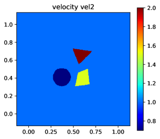
(b)

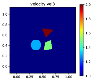
(c)

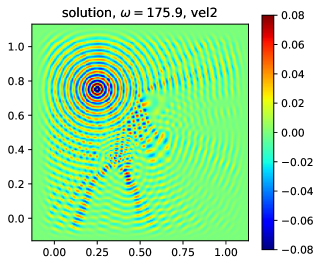
(d)

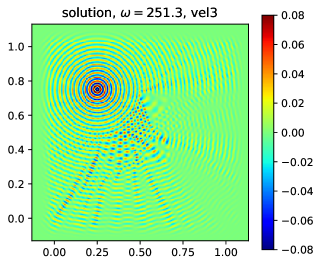
Figure 1. Two velocity models (a,b) and solutions in these models (c,d). A relatively small example of $240\times 240$ was used so that the wavefield oscillations are still visible.

(a)

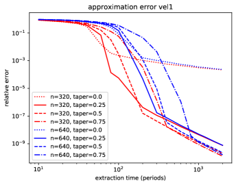
(b)

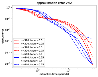
(c)

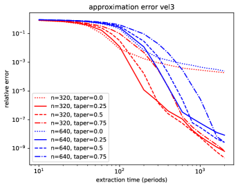
Figure 2. Convergence behavior of large time approximate solutions. Note the different scales in figure (b).

GMRES convergence for the three velocity models of size 640 gridpoints (excluding damping layers) are given in Figure 3. In each case the number of periods of the preconditioner was varied. In Figures 3(a-c) the taper parameter was 0.25 and both the error indicator from GMRES and the true error are plotted. In Figure 3(d) the GMRES error was plotted and the taper parameter was varied. On the x axis, the number of iterations times the number of periods per iteration was displayed. This is roughly, but not quite proportional to the cost, the main difference being that one more preconditioner application is needed for the right-hand side in the preconditioned system. In velocity models 1 and 3, there was no speedup compared to the direct application of the time-domain solver. Neither was the method much slower. However, in the resonant velocity model (velocity model 2), the performance using GMRES was substantially better than when the time-domain solver was used directly.

In the examples about 50 to 100 periods for the preconditioner worked best. This is approximately the size of the example in wavelenghts.

(a)

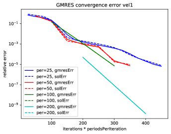
(b)

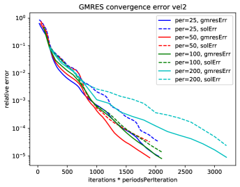
(c)

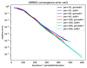
(d)

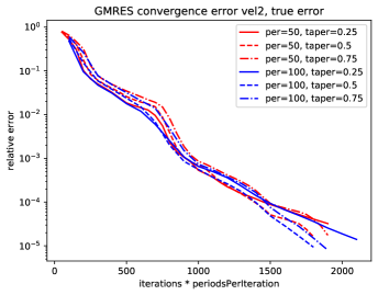
Figure 3. Preconditioned GMRES convergence for different models and different parameter choices

It is confirmed here that, in case of resonances, long time simulation (i.e. applying the limiting amplitude principle directly) leads to poor convergence. For our time-domain preconditioner, a substantial speedup can be obtained by using Krylov accelleration and a smooth window function. Exact controllability is another way of obtaining a speedup, cf. [10, Fig. 7]. How these two methods compare is difficult to say based on what is published. Poor convergence in case of resonances has also been observed in examples using WaveHoltz [1, Fig 4.12(b)] and other iterative methods.

5.2. Examples in 3-D

We also studied the performance of the algorithm in three dimensions. In this case, the velocity model was the SEG/EAGE Salt Model. In this case our goal was to obtain a first estimate of the computational cost of the method. A minimum of 6 gridpoints per wavelength was used. The Julia/C code was run on a 2019 MacBook Pro with a 2.6 GHz 6-core Intel i7 processor and 16 GB main memory. A GMRES error reduction with a factor $10^{-5}$ was required. The results are in Table 2.

physical frequency	2.5 Hz	4 Hz	6 Hz
problem size	$200\times 200\times 106$	$280\times 280\times 130$	$392\times 392\times 165$
degrees of freedom	4.24 e6	1.02 e7	2.54 e7
time steps/period	8	8	8
periods/iteration	25	40	60
taper parameter	0.25	0.25	0.25
iterations	6	6	6
computation time	45 s	166 s	601 s

Table 2. Computational results for the SEG/EAGE Salt model

5.3. Comparison with diagonally preconditioned GMRES

velocity model		diagonal precon		time-domain precon
name	size	#iterations (time)	solerr	#timesteps (time)	solerr
vel1	$320\times 320$	938 (8.8 s)	5.1e-5	2000 (6.3 s)	3.0e-6
vel1	$640\times 640$	1761 (61 s)	7.1e-5	3200 (38 s)	9.7e-6
vel2	$320\times 320$	20503 (204 s)	9.7e-4	9600 (33 s)	1.9e-5
vel2	$640\times 640$	56296 (2066 s)	1.8e-4	15600 (201 s)	3.1e-5
vel3	$320\times 320$	1613 (19 s)	3.3e-5	2400 (7.5 s)	4.0e-5
vel3	$640\times 640$	3197 (110 s)	4.8e-5	3600 (51 s)	3.8e-5

Table 3. Comparison of time-domain preconditioner with a diagonal preconditioner

In Table 3 a comparison between the time-domain preconditioner and diagonally preconditioned GMRES is made. In both cases the number of matrix applications, the computation time and the error compared to the true solution is displayed. The computations were done in Julia.

Diagonally preconditioned GMRES is consistently slower. This is because per matrix application, the diagonally preconditioned GMRES method involves more work, since the vectors spanning the Krylov subspace must be manipulated. In specific scenarios there are more advantages of the time-domain preconditioner. When GPUs are used it is an advantage that the Krylov subspace is manipulated infrequently, which means that the Krylov subspace doesn’t have to be stored in the scarce device memory. In inner-outer iterative methods the time-domain preconditioner could be used as an inner method, with the advantage that it is linear.

6. Explicit scheme for non-diagonal damping

If the matrix $B$ in (13) is non-diagonal, the associated time-stepping method becomes implicit, which is not practical for a hyperbolic time-dependent system. Here we introduce a time-integrator that is explicit even in the case of non-diagonal damping by following similar steps as in section 2. Possible applications are time-harmonic PDE’s discretized using standard finite elements and finite difference discretizations with PML boundary layers. The associated time integrator has stricter CFL conditions and is therefore only proposed for the case that $B$ is non-diagonal.

6.1. Definition of the method

The starting point of our frequency adapted backward differences damped leapfrog scheme is a straightforward modification of (13) in which backward differences are used to discretize the damping term

(144) $$\frac{1}{\Delta t^{2}}\left(u_{n+1}-2u_{n}+u_{n-1}\right)+\frac{B}{\Delta t}\left(u_{n}-u_{n-1}\right)+Au_{n}=f_{n}.$$

The associated time integrator will be called backward differences damped leapfrog.

Definition 5.

Let $K,L$ and $g_{n}$ be as in (14). Backward differences damped leapfrog will be defined as the time integrator given by

(145) $$u_{n+1}=I_{\rm bd}(u_{n},u_{n-1},f_{n}):=(2-K-L)u_{n}-(I-L)u_{n-1}+g_{n}.$$

By choosing $K$, $L$ differently, the resulting time integrator can be made exact for time-harmonic signals of frequency $\omega$. This is shown in the following Proposition, which is an equivalent of Proposition 1. The associated time integration method will be denoted by $I_{\rm abd}$.

Proposition 4.

Let $u_{n}$ and $f_{n}$ be related to $U,F\in{\mathbb{C}}^{N}$ by

(146) $$u_{n}=e^{i\omega n\Delta t}U,\qquad f_{n}=e^{i\omega n\Delta t}F$$

and let $\alpha$ and $\beta$ be as defined in (19). Then $U,F$ satisfy (11) if and only if $u_{n}$, $f_{n}$ satisfy

(147) $$\frac{1}{\Delta t^{2}}\left(u_{n+1}-2u_{n}+u_{n-1}\right)+\frac{\hat{B}}{\Delta t}\left(u_{n}-u_{n-1}\right)+\hat{A}u_{n}=\alpha^{-1}f_{n},$$

where

(148) $$\hat{A}=\alpha^{-1}A-\frac{\beta(1-\cos(\omega\Delta t))}{\alpha\Delta t}B,\qquad\text{ and }\qquad\hat{B}=\alpha^{-1}\beta B.$$

Proof.

To prove this claim, $\hat{A}$, $\hat{B}$ and $\hat{c}$ will be constructed such that

(149) $$\frac{1}{\Delta t^{2}}\left(u_{n+1}-2u_{n}+u_{n-1}\right)+\frac{1}{\Delta t}\hat{B}\left(u_{n}-u_{n-1}\right)+\hat{A}u_{n}=\hat{c}f_{n},$$

if and only if (11). Inserting $u_{n}=Ue^{in\omega\Delta t}$ into (149), results in

(150) $$\left[\frac{2\cos(\omega\Delta t)-2}{\Delta t^{2}}+\frac{i\,\sin(\Delta t\omega)}{\Delta t}\hat{B}+\frac{1-\cos(\Delta t\omega)}{\Delta t}\hat{B}+\hat{A}\right]Ue^{in\omega\Delta t}=\hat{c}e^{in\omega\Delta t}F.$$

Using the definitions of $\alpha$ and $\beta$ and multiplying by $\alpha$ results in the equivalent equation

(151) $$\left[-\omega^{2}+i\omega\frac{\alpha}{\beta}\hat{B}+\frac{\alpha(1-\cos(\Delta t\omega))}{\Delta t}\hat{B}+\alpha\hat{A}\right]U=\alpha\hat{c}F.$$

This is equivalent to (11) if $\hat{c}=\alpha^{-1}$ and $\hat{A}$ and $\hat{B}$ are defined as in (148). ∎

Definition 6.

Frequency adapted backward differences damped leapfrog will be defined as the time integrator given by

(152) $$u_{n+1}=I_{\rm abd}(u_{n},u_{n-1},f_{n}):=(2-K-L)u_{n}-(I-L)u_{n-1}+g_{n}.$$

where $K$, $L$ and $g_{n}$ are given by

(153) $$K={} \frac{\Delta t^{2}}{\alpha}A-\frac{\Delta t\,\beta(1-\cos(\omega\Delta t))}{\alpha}B\qquad$$

$$L={} \frac{\beta\Delta t}{\alpha}B,$$

$$g_{n}={} \frac{\Delta t^{2}}{\alpha}f_{n}$$

We proceed by discussing the choice of $A$, $B$, $\omega$ and $\Delta t$. Obviously we still have (29). The requirements for $\omega$ and $\Delta t$ should follow from stability conditions for $I_{\rm abd}$, cf. subsection 2.2. These stability conditions are (16) and

(154) $$\text{$4I-K-2L$ is positive definite},$$

as shown in subsection 6.2 below.

The method for choosing $\omega$ and $\Delta t$ is somewhat more complicated than in subsection 2.2, because the stability requirement leads to two conditions that both involve $\omega$ and $\Delta t$. It is convenient to use $\omega\Delta t$ and $\Delta t$ as parameters instead of $\omega$ and $\Delta t$. The parameter $\omega\Delta t$ should be between 0 and $\pi$. Given $\omega\Delta t$ the following expression for $\omega^{2}$ can be derived from the condition that $K$ is positive semidefinite and equation (153)

(155) $$\omega^{2}=-\lambda_{\rm min}(\operatorname{Re}H)+\frac{\beta}{\omega\Delta t}(1-\cos(\omega\Delta t))\lambda_{\rm max}(\operatorname{Im}H)$$

(instead of $\lambda_{\rm min}(\operatorname{Re}H)$ and $\lambda_{\rm max}(\operatorname{Im}H)$ lower and upper bounds can be used respectively). From the condition that $4I-K-2L$ is positive definite we then get the following scalar condition

(156) $$\frac{(\omega\Delta t)^{2}}{\alpha}\left(\frac{\lambda_{\rm max}(\operatorname{Re}H)}{\omega^{2}}+1\right)+\frac{\beta}{\alpha}(1+\cos(\omega\Delta t))\frac{\lambda_{\rm max}(\operatorname{Im}H)}{\omega^{2}}<4.$$

The following is a stronger inequality than (156)

(157) $$\left(\frac{\lambda_{\rm max}(\operatorname{Re}H)}{-\lambda_{\rm min}(\operatorname{Re}H)}+1\right)(\omega\Delta t)^{2}+2\frac{\lambda_{\rm max}(\operatorname{Im}H)}{-\lambda_{\rm min}(\operatorname{Re}H)}\omega\Delta t<4.$$

From here a value of $\omega\Delta t$ can be obtained that satisfies the conditions by solving a simple quadratic equation. If a larger value of $\omega\Delta t$ is desired, one can look numerically for a value as large as possible for which (156) is still satisfied.

The time-domain approximate solution operator is defined similarly as in Definition 4.

Definition 7.

Let $\chi$ be an admissible $C^{\infty}$ window function and let $T$ be a positive real constant, such that $n_{\rm steps}:=2\pi\omega^{-1}T/\Delta t$ is an integer. For $F\in{\mathbb{C}}^{N}$, let

(158) $$f_{n}=f(n\Delta t),\qquad f(t)=\chi(1-\frac{t}{2\pi\omega^{-1}T})e^{i\omega t}F.$$

The time-domain approximate solution operator for $H$ associated with the integrator $I_{\rm abd}$ is the linear map $S_{T}^{\rm abd}:{\mathbb{C}}^{N}\to{\mathbb{C}}^{N}$ defined by

(159) $$S_{T}^{\rm abd}F=e^{-i2\pi T}u_{n_{\rm steps}},$$

where $u_{n}$, $n=0,1,\ldots,n_{\rm steps}$ is given by

(160) $$u_{n+1}=I_{\rm abd}(u_{n},u_{n-1},f_{n}),\qquad u_{0}=0.$$

6.2. Analysis

To establish stability of backward differences damped leapfrog, one can study the growth of solutions to the recursion

(161) $$u_{n+1}+(-2+K+L)u_{n}+(I-L)u_{n-1}=0$$

using the energy function

(162) $$E_{\rm bd}(n-1/2)={} \langle u_{n}-u_{n-1},(4I-K)(u_{n}-u_{n-1})\rangle+\langle u_{n}+u_{n-1},K(u_{n}+u_{n-1})\rangle$$

$$-2\langle u_{n}-u_{n-1},L(u_{n}-u_{n-1})\rangle.$$

The following conclusions can be drawn.

1. If $K$ and $4I-K-2L$ are positive definite, then $E_{\rm bd}$ is equivalent to a norm on ${\mathbb{R}}^{2N}$. If $L=0$ then $E_{\rm bd}$ is conserved and solutions remain bounded if $t\to\pm\infty$. If $L$ is positive semidefinite then $\Delta E_{\rm bd}(n)\leq 0$ and solutions remain bounded if $t\to\infty$.

2. If instead $K$ is positive semidefinite with one or more zero eigenvalues and $4I-K-2L$ is positive definite, then $E_{\rm bd}$ is not equivalent to a norm. If $L=0$ then $E_{\rm bd}$ is conserved and solutions grow at most linearly if $t\to\pm\infty$, If $L$ is positive semidefinite, then $\Delta E_{\rm bd}(n)\leq 0$ and solutions grow at most linearly if $t\to\infty$.

For $S_{\rm abd}$ results similar to Theorems 3 and 4 can be obtained by following the same method of proof. The equivalent of (66) is

(163) $$C_{\rm abd}(u)(t)=\frac{\alpha}{\Delta t^{2}}\left[u(t+\Delta t)+(-2+K+L)u(t)+(I-L)u(t-\Delta t)\right]$$

where $K,L$ are as defined in (153). A causal Green’s function $\Phi_{\rm abd}$ is defined satisfying

(164) $$C_{\rm abd}\Phi_{\rm abd}(t)=I\delta(t),\qquad\text{and}\qquad\Phi_{\rm abd}(t)=0\text{ if }t\leq 0,$$

The following theorems are proved in the same ways as theorems 3 and 4

Theorem 6.

Assume $\psi_{\epsilon}$ and $\Phi_{\rm abd}$ are as just defined, then

(165) $$S_{T}^{\rm abd}=\psi_{1/T}\ast\widehat{\Phi}_{\rm abd}(\omega).$$

Theorem 7.

If

(166) $$H=-\omega^{2}I+i\omega B+A$$ is non-singular

and $A,B,\omega$ and $\Delta t$ are such that $K$, $L$ defined in (153) satisfy the stability conditions (16) and (154) then

(167) $$\lim_{T\to\infty}S_{T}^{\rm abd}=H^{-1}.$$

7. Concluding remarks

In this paper we constructed a time-domain preconditioner for indefinite linear systems that come from discretizing time-harmonic wave equations, and studied its properties and behavior analytically and with numerical examples. It should be emphasized that the method does not compute in the physical time domain. We call it a time-domain method, because of the similarity with classical time-domain methods for time-harmonic waves. For the practical application it would be useful to have further examples, with different matrices $H$ and a comparison with alternatives. We will make a few brief remarks in this direction.

First it is clear that the method requires relatively little memory, compared to alternatives that use LU (or LDL^T) decompositions, such as domain-decomposition and direct methods, see [19, 15] and references in [8]. In the 3-D implementation here, with GMRES with restart $m=10$, most memory was used for the approximately $m+2$ complex double precision vectors needed for GMRES. This was in part because the timestepping was done in single precision, and using real fields. In principle, memory use could be somewhat reduced by setting $m=5$ or using a different iterative method like BiCGSTAB.

For finite element discretizations the cost in general will be different. These methods often have stricter CFL bounds, there may be more nonzero matrix elements, and the use of unstructured meshes may also influence efficiency. On the other hand, the size of the grid cells can be adapted to the local velocity so that the number of grid cells can be smaller.

It is difficult to compare performance of different methods, as methods are run on different computer systems, with different examples and implementations are optimized to different degrees. We refer to [1, 7, 13, 15, 19, 23, 25] for some alternative methods. We believe that computation times of the method as outlined are modest, and there is potential for further improvements, by using GPUs or by reorganizing the code to better make use of cached data. It remains challenging to get the most out of modern computer hardware in time-domain finite-difference and finite-element simulations. We hope that recent developments in this area, cf. [14], will lead to further improvements.

Appendix A Additional material for subsection 3.2

In case of variable coefficients, the 27 point optimized finite-differences discretization used in subsection 3.2 is done in a quasi-finite-element way that we now explain. This is consistent with [18].

We first define some notation. In this appendix, three dimensional indices are denoted by greek letters, e.g. $\alpha=(\alpha_{1},\alpha_{2},\alpha_{3})$. A grid cell will have the same index as the point in the lower (in all dimensions) corner. The set of corners of a grid cell will be denoted by $C(\alpha)$. We define

(168) $$\Delta(\alpha,\beta)=|\alpha_{1}-\beta_{1}|+|\alpha_{2}-\beta_{2}|+|\alpha_{3}-\beta_{3}|.$$

If $\alpha,\beta$ are two corner points of a grid cell, then this number is 0 if they are the same and 1, 2, or 3 if they are opposite points on an edge, face, or the cell itself respectively. We define

(169) $$\tilde{f}_{s}\left(\frac{kh}{2\pi}\right)=\frac{1}{2^{3-s}}f_{s}\left(\frac{kh}{2\pi}\right)$$

In case of variable coefficients, the coefficient $k$ will be constant on grid cells, its value is denoted by $k^{(\alpha)}$

The matrix $\operatorname{Re}H$ will be associated with a bilinear form

(170) $$\mathcal{H}(v,u)=\sum_{\text{cells $\alpha$}}\mathcal{H}_{\rm cell}(\alpha;v,u).$$

The contribution for a single cell is given by

(171) $$\mathcal{H}_{\rm cell}(\alpha;v,u)=\sum_{\beta,\gamma\in C(\alpha)}\tilde{f}_{\Delta(\beta,\gamma)}\left(\frac{hk^{(\alpha)}}{2\pi}\right)v^{(\beta)}u^{(\gamma)}$$

For each cell we have

(172) $$\mathcal{H}_{\rm cell}(\alpha;u,u)\geq-(k^{(\alpha)})^{2}\frac{1}{8}\sum_{\beta\in C(\alpha)}\left|u^{(\beta)}\right|^{2}.$$

An expression for $\lambda_{\rm min}(\operatorname{Re}H)$ follows straightforwardly from this. For an upperbound for $\lambda_{\rm max}(\operatorname{Re}H)$ one can use (51) with $k$ replaced by $k_{\rm min}$.

Appendix B Fourier transform of the unit step function on ${\mathbb{Z}}$

In this appendix we consider the Fourier transform of a discrete unit step function. Although this is a standard result, we could not locate a proof and included one here.

Proposition 5.

Denote by $U(n)$, $n\in{\mathbb{Z}}$ the unit step function

(173) $$U(n)=\left\{\begin{array}[]{ll}0&\text{if $n\leq 0$}\\ 1&\text{if $n>0$}\end{array}\right.$$

The Fourier transform of $U$ equals

(174) $$\widehat{U}(\nu)=\pi\delta(\nu)-\frac{i}{2}\cot(\frac{\nu}{2})-\frac{1}{2}.$$

Here the distribution associated with $\cot$ is defined by the principal value integral.

Proof.

Consider the first the Fourier transform of $g(n)=\operatorname{sgn}(n)$. We claim it is given by

(175) $$\widehat{g}(\nu)=\frac{1}{1-e^{-i\nu}}-\frac{1}{1-e^{i\nu}},$$

which is interpreted as a distribution using the principal value integral. Indeed, consider the inverse Fourier transform of our candidate for $\widehat{g}$

(176) $$\frac{1}{2\pi}\int_{-\pi}^{\pi}\left(\frac{e^{in\nu}}{1-e^{-i\nu}}-\frac{e^{in\nu}}{1-e^{i\nu}}\right)\,d\nu.$$

For each of the two contributions the real part is even and the imaginary part is odd in $\nu$. Therefore, for each of the two contributions only the real part contributes to the integral and the integral equals

(177) $$\int_{-\pi}^{\pi}\frac{e^{in\nu}-e^{-in\nu}}{1-e^{-i\nu}}\,d\nu=\left\{\begin{array}[]{ll}0&\text{if $n=0$}\\ \frac{1}{2\pi}\int_{-\pi}^{\pi}\left(e^{in\nu}+e^{i(n-1)\nu}+\ldots+e^{-i(n-1)\nu}\right)\,d\nu=1&\text{if $n>0$}\\ -\frac{1}{2\pi}\int_{-\pi}^{\pi}\left(e^{i(-n)\nu}+e^{i(-n-1)\nu}+\ldots+e^{-i(-n-1)\nu}\right)\,d\nu=-1&\text{if $n<0$}\end{array}\right.$$

Simple manipulations show that $\widehat{g}$ can also be written as $\widehat{g}=-i\cot(\frac{\nu}{2})$. The unit step function can be written as

(178) $$U(n)=\frac{1}{2}+\frac{1}{2}\operatorname{sgn}(n)-\frac{1}{2}\delta_{0,n}$$

The Fourier transform is hence as given in (174). ∎

References

• [1] D. Appelo, F. Garcia, and O. Runborg. Waveholtz: Iterative solution of the Helmholtz equation via the wave equation, 2019.
• [2] I. Babuška, F. Ihlenburg, E. T. Paik, and S. A. Sauter. A generalized finite element method for solving the Helmholtz equation in two dimensions with minimal pollution. Comput. Methods Appl. Mech. Engrg., 128(3-4):325–359, 1995.
• [3] J. Berland, C. Bogey, and C. Bailly. Low-dissipation and low-dispersion fourth-order Runge–Kutta algorithm. Computers & Fluids, 35(10):1459–1463, 2006.
• [4] B.R. Vainberg. Limiting-amplitude principle. Encyclopedia of Mathematics. URL: http://www.encyclopediaofmath.org/index.php?title=Limiting-amplitude_principle&oldid=44712. Accessed on 2020-05-4.
• [5] M.-O. Bristeau, R. Glowinski, and J. Périaux. Controllability methods for the computation of time-periodic solutions; application to scattering. Journal of Computational Physics, 147(2):265–292, 1998.
• [6] A. Brünger, C. L. Brooks III, and M. Karplus. Stochastic boundary conditions for molecular dynamics simulations of st2 water. Chemical physics letters, 105(5):495–500, 1984.
• [7] H. Calandra, S. Gratton, X. Pinel, and X. Vasseur. An improved two-grid preconditioner for the solution of three-dimensional Helmholtz problems in heterogeneous media. Numer. Linear Algebra Appl., 20(4):663–688, 2013.
• [8] M. J. Gander and H. Zhang. A class of iterative solvers for the helmholtz equation: Factorizations, sweeping preconditioners, source transfer, single layer potentials, polarized traces, and optimized schwarz methods. Siam Review, 61(1):3–76, 2019.
• [9] M. Grote and T. Mitkova. Explicit local time-stepping methods for time-dependent wave propagation. arXiv preprint arXiv:1205.0654, 2012.
• [10] M. J. Grote, F. Nataf, J. H. Tang, and P.-H. Tournier. Parallel controllability methods for the helmholtz equation. Computer Methods in Applied Mechanics and Engineering, 362:112846, 2020.
• [11] M. J. Grote and J. H. Tang. On controllability methods for the helmholtz equation. Journal of Computational and Applied Mathematics, 358:306–326, 2019.
• [12] O. Holberg. Computational aspects of the choice of operator and sampling interval for numerical differentiation in large-scale simulation of wave phenomena. Geophys. Prosp., 35(6):629–655, 1987.
• [13] X. Liu, Y. Xi, Y. Saad, and M. V. de Hoop. Solving the 3d high-frequency helmholtz equation using contour integration and polynomial preconditioning. arXiv preprint arXiv:1811.12378, 2018.
• [14] M. Louboutin, M. Lange, F. Luporini, N. Kukreja, P. A. Witte, F. J. Herrmann, P. Velesko, and G. J. Gorman. Devito (v3. 1.0): an embedded domain-specific language for finite differences and geophysical exploration. Geoscientific Model Development, 12(3):1165–1187, 2019.
• [15] J. Poulson, B. Engquist, S. Li, and L. Ying. A parallel sweeping preconditioner for heterogeneous 3d helmholtz equations. SIAM Journal on Scientific Computing, 35(3):C194–C212, 2013.
• [16] A. W. Sandvik. Numerical solutions of classical equations of motion. http://physics.bu.edu/py502/lectures3/cmotion.pdf. Lecture Notes Boston University PY 502, accessed: 2020-01-13.
• [17] T. Schlick. Molecular modeling and simulation: an interdisciplinary guide: an interdisciplinary guide, volume 21. Springer Science & Business Media, 2010.
• [18] C. C. Stolk. A dispersion minimizing scheme for the 3-d Helmholtz equation based on ray theory. Journal of computational Physics, 314:618–646, 2016.
• [19] C. C. Stolk. An improved sweeping domain decomposition preconditioner for the Helmholtz equation. Advances in Computational Mathematics, 43(1):45–76, 2017.
• [20] C. C. Stolk, M. Ahmed, and S. K. Bhowmik. A multigrid method for the Helmholtz equation with optimized coarse grid corrections. SIAM Journal on Scientific Computing, 36(6):A2819–A2841, 2014.
• [21] G. Sutmann. Compact finite difference schemes of sixth order for the helmholtz equation. Journal of Computational and Applied Mathematics, 203(1):15–31, 2007.
• [22] C. K. Tam and J. C. Webb. Dispersion-relation-preserving finite difference schemes for computational acoustics. Journal of computational physics, 107(2):262–281, 1993.
• [23] M. Taus, L. Zepeda-Núñez, R. J. Hewett, and L. Demanet. L-sweeps: A scalable, parallel preconditioner for the high-frequency helmholtz equation. arXiv preprint arXiv:1909.01467, 2019.
• [24] E. Turkel, D. Gordon, R. Gordon, and S. Tsynkov. Compact 2D and 3D sixth order schemes for the Helmholtz equation with variable wave number. Journal of Computational Physics, 232(1):272 – 287, 2013.
• [25] S. Wang, M. V. De Hoop, and J. Xia. On 3d modeling of seismic wave propagation via a structured parallel multifrontal direct Helmholtz solver. Geophys. Prospect, 59:857–873, 2011.
• [26] L. Zschiedrich, S. Burger, B. Kettner, and F. Schmidt. Advanced finite element method for nano-resonators. In Physics and Simulation of Optoelectronic Devices XIV, volume 6115, page 611515. International Society for Optics and Photonics, 2006.