Merging of transport theory with TDHF: multinucleon transfer in U+U collisions

Abstract

Multinucleon transfer mechanism in the collision of ${}^{238}\text{U}+{}^{238}\text{U}$ system is investigated at $E_{\text{c.m.}}=833$ MeV in the framework of the quantal diffusion description based on the stochastic mean-field approach (SMF). Double cross-sections $\sigma(N,Z)$ as a function of the neutron and proton numbers, the cross-sections $\sigma(Z)$ and $\sigma(A)$ as a function of the atomic numbers and the mass numbers are calculated for production of the primary fragments. The calculation indicates the ${}^{238}\text{U}+{}^{238}\text{U}$ system may be located at an unstable equilibrium state at the potential energy surface with a slightly negative curvature along the beta stability line on the $(N,Z)-$plane. This behavior may lead to rather large diffusion along the beta stability direction.

I INTRODUCTION

It has been recognized that multinucleon transfer in heavy-ion collisions involving massive nuclei provide a suitable mechanism for synthesizing new neutron rich heavy nuclei Adamian et al. (2003); Valery Zagrebaev and Walter Greiner (2007); Aritomo (2009); Adamian et al. (2010); Barrett et al. (2015); Devaraja et al. (2015); Zhao et al. (2016); Sekizawa and Yabana (2016); Feng (2017); Sekizawa (2017); Kazuyuki Sekizawa (2019); Mun et al. (2019); Saiko and Karpov (2019); Jiang and Wang (2020). For this purpose, experimental investigations have been carried out in heavy-ion collision with actinide targets near barrier energies Kozulin et al. (2012); Kratz et al. (2013); Watanabe et al. (2015); Desai et al. (2019). Collisions of massive systems near barrier energies predominantly lead to dissipative deep-inelastic reactions and quasi-fission reactions. In dissipative collisions the most part of the bombarding energy is converted into the internal excitations, and the multinucleon transfer occurs between the projectile and target nuclei. A number of experimental and theoretical investigations have been made of the multinucleon transfer mechanism in heavy-ion collisions near barrier energies. The multi dimensional phenomenological Langevin type dynamical approaches have been developed for describing dissipative collisions between massive nuclear systems Valery Zagrebaev and Walter Greiner (2008); Zagrebaev and Greiner (2011); Zagrebaev et al. (2012); Karpov and Saiko (2017); Saiko and Karpov (2019). These phenomenological models provide a qualitative and in some cases semi-quantitative description of the transfer process. Since many years, the time-dependent Hartree-Fock (TDHF) approach has been used for describing the deep-inelastic collisions and the quasi-fission reactions Simenel (2012); Nakatsukasa et al. (2016); Oberacker et al. (2014, 2010); Umar et al. (2015); Kazuyuki Sekizawa (2019); Simenel and Umar (2018). The TDHF provides a microscopic description in terms of Skyrme-type energy density functionals. The mean-field theory provides good a description for the most probable dynamical path of the collective motion at low energy heavy ion-collisions including the one-body dissipation mechanism. However the mean-field theory severely underestimates the fluctuations around the most probable collective path. The particle number projection method of the TDHF indeed shows the fragment mass and charge distributions are largely underestimated for strongly damped collisions Simenel (2010); Sekizawa and Yabana (2016). The fragment mass and charge distributions observed in symmetric collisions provide a good example for the shortcoming of the mean-field description. In the TDHF calculations of the symmetric collisions, the identities of the projectile and target are strictly preserved, i.e., the mass and charge numbers of the final fragments are exactly same as of those at the initial fragments. The experiments, on the other hand, exhibits broad mass and charge distributions of final fragments around their initial values. The dominant aspect of the data is a broad mass and charge distribution around the projectile and target resulting from multinucleon diffusion mechanism. The description of such large fluctuations requires an approach beyond the mean-field theory. The time-dependent RPA approach of Balian and Veneroni provides a possible approach for calculating dispersion of fragment mass and charge distributions and dispersion of other one-body observables Roger Balian and Marcel Vénéroni (1984); Balian and Vénéroni (1985); Broomfield and Stevenson (2008); Williams et al. (2018); Godbey and Umar (2020). However, this approach has severe technical difficulties in applications to the collisions of asymmetric systems. In this work, we employ the quantal diffusion description based on the stochastic mean-field (SMF) approach to calculate double cross-sections $\sigma(N,Z)$, the cross-section as function of mass number $\sigma(A)$ and cross-section as a function of the atomic number $\sigma(Z)$ of the primary fragments in the collisions of the symmetric ${}^{238}\text{U}+{}^{238}\text{U}$ system at $E_{\text{c.m.}}=833$ MeV Ayik (2008); Lacroix and Ayik (2014). In the quantal diffusion description, the transport theoretical concepts are merged with the mean-field description of the TDHF. As a result, it is possible to calculate the transport coefficients of macroscopic variables in terms of the mean-field properties provided by the time-dependent wave functions of the TDHF, which is consistent with the fluctuation-dissipation theorem of the non-equilibrium statistical mechanics. In Sec. II, we present a brief description of the quantal nucleon diffusion description of the multinucleon exchange. In Sec. III, we present results of calculations of the cross-sections for production of the primary fragments, and conclusions are given in Sec. IV. Some calculations details are provided in the Appendices.

II QUANTAL DIFFUSION OF MULTINUCLEON TRANSFERS

In the SMF approach, the dynamics of heavy-ion collisions is described in terms of an ensemble of mean-field events. Each event is determined by the self-consistent mean-field Hamiltonian of that event with the initial conditions specified by the thermal and quantal fluctuations at the initial state. We consider uranium-uranium collisions at bombarding energies near Coulomb barrier. During the collision, the projectile and the target form a di-nuclear complex and interact mainly by multinucleon exchanges. Because of the di-nuclear structure, rather than generating an ensemble of stochastic mean-field events, it is possible to describe the dynamics in terms of several relevant macroscopic variables, such as neutron and proton numbers of the one side of the complex and relative momentum of projectile-like and the target-like fragments. It is possible to deduce the Langevin-type transport description for the macroscopic variables Gardiner (1991); Weiss (1999) and calculate transport coefficients of the macroscopic variables in terms of the TDHF solutions. In this manner, the SMF approach provides a ground for merging transport theory with the mean-field description. For the detail description of the SMF approach and the applications, we refer the reader the previous publications Ayik et al. (2017, 2018); Yilmaz et al. (2018); Ayik et al. (2019); Sekizawa and Ayik (2020); Yilmaz et al. (2020). Here we take the neutron $N_{1}^{\lambda}$ and the proton $Z_{1}^{\lambda}$ numbers of the projectile-like fragments as the macroscopic variables. In each event $\lambda$, the neutron and proton numbers are determined by integrating the nucleon density over the projectile side of the window between the colliding nuclei,

$$\left(\begin{array}[]{c}{N_{1}^{\lambda}(t)}\\ {Z_{1}^{\lambda}(t)}\end{array}\right)=\int d^{3}r\Theta\left[x^{\prime}(t)\right]\left(\begin{array}[]{c}{\rho_{n}^{\lambda}(\vec{r},t)}\\ {\rho_{p}^{\lambda}(\vec{r},t)}\end{array}\right),$$ (5)

where $x^{\prime}(t)=[y-y_{0}(t)]\sin\theta+[x-x_{0}(t)]\cos\theta$. The $(x,y)$-plane represents the reaction plane with $x$-axis being the beam direction in the center of mass frame (COM) of the colliding ions. The window plane is perpendicular to the symmetry axis and its orientation is specified by the condition $x^{\prime}(t)=0$. In this expression, $x_{0}(t)$ and $y_{0}(t)$ denote the coordinates of the window center relative to the origin of the COM frame, $\theta(t)$ is the smaller angle between the orientation of the symmetry axis and the beam direction. We neglect fluctuations in the orientation of the window and determine the mean evolution of the window dynamics by diagonalizing the mass quadrupole moment of the system for each impact parameter $b$ or the initial orbital angular momentum $\ell$, as described in Appendix A, of Ref. Ayik et al. (2018). In terms of the TDHF description, it is possible to determine time evolution of the rotation angle $\theta(t)$ of the symmetry axis. The coordinates $x_{0}(t)$ and $y_{0}(t)$ of the center point of the window are located at the center of the minimum density slice on the neck between the colliding ions. Since uranium is a deformed nucleus, the outcome of the collisions depends on the relative orientation of the projectile and target. In the present work, we consider two specific collision geometry: (i) the side-side collisions in which deformation axes of the both the projectile and the target are perpendicular to the beam direction and (ii) the tip-tip is collisions in which deformation axes of the both the projectile and the target are parallel to the beam direction. As an example, Fig. 1 shows the density profile in the tip-tip geometry (left panel) and in the side-side geometry (right panel) of the ${}^{238}\text{U}+{}^{238}\text{U}$ system at $E_{\text{c.m.}}=833$ MeV with the initial orbital angular momentum $\ell=300\hbar$ at times $t=300$ fm/c , $t=500$ fm/c and $t=700$ fm/c. The window plane and symmetry axis of the di-nuclear complex are indicated by thick and dashed lines in frame (b) of the left panel. In the calculation of this figure and in the calculations presented in the rest of the article, we employ the TDHF code developed by Umar et al. Umar et al. (1991); Umar and Oberacker (2006) using the SLy4d Skyrme functional Ka–Hae Kim et al. (1997). In the following, all quantities are calculated for a given initial orbital angular momentum $\ell$, but for the purpose of clarity of expressions, we do not attach the angular momentum label to the quantities. The quantities in Eq. (5)

$$\rho_{\alpha}^{\lambda}(\vec{r},t)=\sum_{ij\in\alpha}\Phi_{j}^{*\alpha}(\vec{r},t;\lambda)\rho_{ji}^{\lambda}\Phi_{i}^{\alpha}(\vec{r},t;\lambda)\;,$$ (6)

are the neutron and proton densities in the event $\lambda$ of the ensemble. Here, and in the rest of the article, we use the notation $\alpha=n,p$ for the neutron and proton labels. According to the main postulate of the SMF approach, the elements of the initial density matrix are specified by uncorrelated Gaussian distributions with the mean values $\bar{\rho}_{ji}^{\lambda}=\delta_{ji}n_{j}$ and the second moments determined by,

$$\overline{\delta\rho_{ji}^{\lambda}\delta\rho_{i^{\prime}j^{\prime}}^{\lambda}}=\frac{1}{2}\delta_{ii^{\prime}}\delta_{jj^{\prime}}\left[n_{i}(1-n_{j})+n_{j}(1-n_{i})\right],$$ (7)

where $n_{j}$ are the average occupation numbers of the single-particle wave functions at the initial state. At zero initial temperature, these occupation numbers are zero or one, and at finite initial temperatures the occupation numbers are given by the Fermi-Dirac functions. Here and below, the bar over the quantity indicates the average over the generated ensemble.

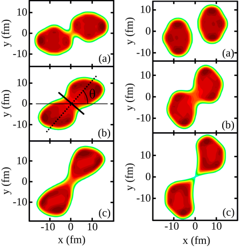
Figure 1: The density profile and the collision geometry of the ${}^{238}\text{U}+{}^{238}\text{U}$ collisions at $E_{\text{c.m.}}=833$ MeV with the initial orbital angular momentum $\ell=300\hbar$ at times $t=300$ fm/c , $t=500$ fm/c and $t=700$ fm/c at tip-tip geometry (left panel) and side-side geometry (right panel).

Below, we briefly discuss the derivation of the Langevin equations for the neutron and proton numbers of the projectile-like fragments, for further details we refer the reader to Refs. Ayik et al. (2017, 2018); Yilmaz et al. (2018); Ayik et al. (2019). The rate of changes the neutron and the proton numbers of the projectile-like fragment are given by,

$$\frac{d}{dt}\left(\begin{array}[]{c}{N_{1}^{\lambda}(t)}\\ {Z_{1}^{\lambda}(t)}\end{array}\right)=-\int d^{3}r\Theta\left[x^{\prime}(t)\right]\left(\begin{array}[]{c}{\vec{\nabla}\cdot\vec{j}_{n}^{\lambda}(t)}\\ {\vec{\nabla}\cdot\vec{j}_{p}^{\lambda}(t)}\end{array}\right).$$ (12)

In obtaining this expression we neglect a term arising from the rate of change of the position and the rotation of the window plane and employ the continuity equation, with the fluctuating neutron and proton current densities

$$\vec{j}_{\alpha}^{\lambda}(\vec{r},t)==\frac{\hbar}{m}\sum_{ij\in\alpha}\text{Im}\left(\Phi_{j}^{*\alpha}(\vec{r},t;\lambda)\vec{\nabla}\Phi_{i}^{\alpha}(\vec{r},t;\lambda)\rho_{ji}^{\lambda}\right).$$ (13)

By carrying out a partial integration, we obtain a set of coupled Langevin equations for the macroscopic variables $N_{1}^{\lambda}(t)$ and $Z_{1}^{\lambda}(t)$,

$$\frac{d}{dt}\left(\begin{array}[]{c}{N_{1}^{\lambda}(t)}\\ {Z_{1}^{\lambda}(t)}\end{array}\right)=\int d^{3}rg(x^{\prime})\left(\begin{array}[]{c}{\hat{e}\cdot\vec{j}_{n}^{\lambda}(\vec{r},t)}\\ {\hat{e}\cdot\vec{j}_{p}^{\lambda}(\vec{r},t)}\end{array}\right)=\left(\begin{array}[]{c}{v_{n}^{\lambda}(t)}\\ {v_{p}^{\lambda}(t)}\end{array}\right),$$ (20)

with $\hat{e}$ as the unit vector along the symmetry axis with components $\hat{e}_{x}=\cos\theta$ and $\hat{e}_{y}=\sin\theta$. In the integrand, we replace the delta function by a smoothing function $\delta(x^{\prime})\to g(x^{\prime})$ in terms of a Gaussian $g(x)=\left(1/\kappa\sqrt{2\pi}\right)\exp\left(-x^{2}/2\kappa^{2}\right)$ with dispersion $\kappa$. The Gaussian behaves almost like delta function for sufficiently small $\kappa$. In the numerical calculations dispersion of the Gaussian is taken in the order of the lattice side $\kappa=1.0$  fm. The right side of Eq. (20) defines the fluctuating drift coefficients $v_{\alpha}^{\lambda}(t)$ for the neutrons and the protons. There are two different sources for fluctuations of the drift coefficients: (i) Fluctuations due to different set of wave functions in each event $\lambda$. This part of the fluctuations can be approximately described in terms of the fluctuating macroscopic variables as $v_{\alpha}^{\lambda}(t)\to v_{\alpha}\left(N_{1}^{\lambda}(t),Z_{1}^{\lambda}(t)\right)$, and (ii) fluctuations introduced by the stochastic part $\delta\rho_{ji}^{\lambda}=\rho_{ji}^{\lambda}-\delta_{ji}n_{j}$ of the density matrix at the initial state. In this work, we consider small amplitude fluctuations, and linearize the Langevin Eq. (20) around the mean values of the macroscopic variables $\delta N_{1}^{\lambda}=N_{1}^{\lambda}-\overline{N}_{1}$ and $\delta Z_{1}^{\lambda}=Z_{1}^{\lambda}-\overline{Z}_{1}$. The mean values $\overline{N}_{1}=\overline{N_{1}^{\lambda}}$ and $\overline{Z}_{1}=\overline{Z_{1}^{\lambda}}$ are determined by the mean-field description of the TDHF approach. Table 1 and table 2 show the results of the TDHF calculations for the mean values for a set of observable quantities in the collisions of ${}^{238}\text{U}+{}^{238}\text{U}$ system at $E_{\text{c.m.}}=833$ MeV for the range initial orbital angular momentum $\ell=(100-460)\hbar$.

Table 1: Result of TDHF calculations for tip-tip collisions of ${}^{238}\text{U}+{}^{238}\text{U}$ system at $E_{\text{c.m.}}=833$ MeV for final values of mass and charge of the projectile-like ($A_{1}^{f}$, $Z_{1}^{f}$) and target-like fragments ($A_{2}^{f}$, $Z_{2}^{f}$) final orbital angular momentum $\ell_{f}$, total kinetic energy (TKE), total excitation energy $E*$, center of mass $\theta_{\text{c.m.}}$ and laboratory scattering angles ($\theta_{1}^{\text{lab}}$,$\theta_{2}^{\text{lab}}$) for a set initial orbital angular momentum $\ell_{i}$.

$\ell_{i}\,$($\hbar$)	A${}_{1}^{f}$	Z${}_{1}^{f}$	A${}_{2}^{f}$	Z${}_{2}^{f}$	$\ell_{f}\,$($\hbar$)	TKE	E∗	$\theta_{c.m.}$	$\theta_{1}^{lab}$	$\theta_{2}^{lab}$
						(MeV)	(MeV)
100	238	92.0	238	92.0	73.4	527	306	158	48.3	9.55
120	238	92.0	238	92.0	95.4	514	319	154	49.6	11.5
140	238	92.0	238	92.0	114	505	328	149	50.4	13.6
160	238	92.0	238	92.0	132	521	312	149	51.7	13.7
180	238	92.0	238	92.0	153	510	323	138	51.3	18.5
200	238	92.3	238	91.7	172	515	317	132	50.8	20.9
220	238	92.0	238	92.0	177	525	318	129	50.4	22.4
240	238	92.0	238	92.0	182	552	281	126	51.6	24.1
260	238	91.6	238	92.4	185	577	256	123	52.2	25.6
280	238	92.0	238	92.0	189	595	238	120	51.6	27.4
300	238	92.0	238	92.0	201	616	217	116	51.2	29.3
320	238	92.0	238	92.0	225	625	208	113	50.1	31.0
340	238	92.0	238	92.0	245	645	188	109	49.5	32.8
360	238	92.0	238	92.0	271	654	179	106	48.3	34.6
380	238	92.0	238	92.0	333	714	119	101	47.8	37.7
400	238	92.0	238	92.0	374	751	82.3	98.4	47.5	39.5
420	238	92.0	238	92.0	429	797	35.9	96.2	47.4	41.4
440	238	92.0	238	92.0	439	785	48.1	93.4	45.8	42.5
460	238	92.0	238	92.0	491	819	14.1	91.4	45.5	44.1

Table 2: Same as Table 1 for side-side collisions.

$\ell_{i}\,$($\hbar$)	A${}_{1}^{f}$	Z${}_{1}^{f}$	A${}_{2}^{f}$	Z${}_{2}^{f}$	$\ell_{f}\,$($\hbar$)	TKE	E∗	$\theta_{c.m.}$	$\theta_{1}^{lab}$	$\theta_{2}^{lab}$
						(MeV)	(MeV)
100	238	92.3	238	91.7	71.3	658	173	154	62.3	12.5
120	238	92.0	238	92.0	86.5	660	173	149	62.7	14.4
140	238	92.0	238	92.0	99.2	660	173	145	62.0	16.5
160	238	92.0	238	92.0	116	668	165	140	61.3	19.0
180	238	92.0	238	92.0	140	659	174	134	59.3	21.2
200	238	92.1	238	91.9	164	666	167	129	57.8	23.9
220	238	92.0	238	92.0	184	673	160	125	57.6	26.0
240	238	92.0	238	92.0	196	673	160	122	55.5	27.4
260	238	92.0	238	92.0	214	682	214	119	52.2	28.2
280	238	92.0	238	92.0	234	692	141	115	53.4	30.7
300	238	92.0	238	92.0	258	699	134	112	52.1	32.5
320	238	92.0	238	92.0	282	705	128	108	50.8	34.2
340	238	92.0	238	92.0	302	713	120	105	49.8	35.6
360	238	92.0	238	92.0	318	723	110	103	49.1	36.8
380	238	92.0	238	92.0	333	736	96.6	102	48.6	37.8
400	238	92.0	238	92.0	331	751	81.7	99.7	48.1	38.9
420	238	92.0	238	92.0	373	768	65.0	97.8	47.6	40.1
440	238	92.0	238	92.0	393	785	47.6	96.2	47.2	41.2
460	238	92.0	238	92.0	410	802	31.4	94.9	46.9	42.1

The fluctuations evolve according to the linearized coupled Langevin equations,

$$\frac{d}{dt}\left(\begin{array}[]{c}{\delta Z_{1}^{\lambda}}\\ {\delta N_{1}^{\lambda}}\end{array}\right)= \left(\begin{array}[]{c}{\frac{\partial v_{p}}{\partial Z_{1}}(Z_{1}^{\lambda}-\overline{Z}_{1})+\frac{\partial v_{p}}{\partial N_{1}}(N_{1}^{\lambda}-\overline{N}_{1})}\\ {\frac{\partial v_{n}}{\partial Z_{1}}(Z_{1}^{\lambda}-\overline{Z}_{1})+\frac{\partial v_{n}}{\partial N_{1}}(N_{1}^{\lambda}-\overline{N}_{1})}\end{array}\right)$$ (25)

$$+\left(\begin{array}[]{c}{\delta v_{p}^{\lambda}(t)}\\ {\delta v_{p}^{\lambda}(t)}\end{array}\right),$$ (28)

where the derivatives of drift coefficients are evaluated at the mean values $\overline{N}_{1}$ and $\overline{Z}_{1}$. The linear limit provides a good approximation for small amplitude fluctuations and it becomes even better if the driving potential energy has nearly harmonic behavior around the mean values. The stochastic part $\delta v_{\alpha}^{\lambda}(t)$ of drift coefficients given by,

$$\delta v_{\alpha}^{\lambda}(t)=\frac{\hbar}{m}\sum_{ij\in\alpha}\int d^{3}rg(x^{\prime})\text{Im}\left(\Phi_{j}^{*\alpha}(\vec{r},t)\stackrel{{\scriptstyle\frown}}{{e}}\cdot\vec{\nabla}\Phi_{i}^{\alpha}(\vec{r},t)\delta\rho_{ji}^{\lambda}\right).$$ (29)

According to the basic postulate of the SMF approach the stochastic elements of the initial density matrix $\delta\rho_{ji}^{\lambda}$ are specified in terms of uncorrelated distributions, then it follows that the stochastic part of the neutron and proton drift coefficients $\delta v_{\alpha}^{\lambda}(t)$ are determined by uncorrelated Gaussian distributions with variances discussed in the following section.

III MASS AND CHARGE DISTRIBUTIONS OF THE PRIMARY FRAGMENTS

III.1 Quantal diffusion coefficients of neutrons and protons

It is well known that Langevin equation for a macroscopic variable is equivalent to the Fokker-Planck equation for the distribution function of the macroscopic variable and the solution is given by a single Gaussian function Hannes Risken and Till Frank (1996). When there are two coupled Langevin equations, as we have it in Eq. (25), the solution of the Fokker-Planck equation for the distribution function $P\left(N,Z\right)$ of fragments with neutron and proton numbers $\left(N,Z\right)$ is specified by a correlated Gaussian function for each value of the initial orbital angular momentum $\ell$,

$$P(N,Z)=\frac{1}{2\pi\sigma_{NN}\sigma_{ZZ}\sqrt{1-\rho^{2}}}\exp\left[-C\left(N,Z\right)\right].$$ (30)

Here the exponent $C\left(N,Z\right)$ is given by

$$\overline{C}\left(N,Z\right)=\frac{1}{2\left(1-\rho^{2}\right)}$$

$$\times\left[\left(\frac{Z-\overline{Z}}{\sigma_{ZZ}}\right)^{2}-2\rho\left(\frac{Z-\overline{Z}}{\sigma_{ZZ}}\right)\left(\frac{N-\overline{N}}{\sigma_{NN}}\right)+\left(\frac{N-\overline{N}}{\sigma_{NN}}\right)^{2}\right],$$ (31)

with the correlation coefficient $\rho=\sigma_{NZ}^{2}/\sigma_{ZZ}\sigma_{NN}$. In this expression $\overline{N}$ and $\overline{Z}$ are the mean values the neutron and the proton numbers of fragments for each angular momentum determined by the TDHF calculations, and $\sigma_{NN}$, $\sigma_{ZZ}$ and $\sigma_{NZ}$ denote the neutron, proton and mixed dispersions, respectively. Multiplying both side in Eq. (25) by $\delta N_{1}^{\lambda}$ and $\delta Z_{1}^{\lambda}$ and carrying out ensemble averaging, we obtain a couple set of equations for the neutron $\sigma_{NN}^{2}=\overline{\delta N_{1}^{\lambda}\delta N_{1}^{\lambda}}$, the proton $\sigma_{ZZ}^{2}=\overline{\delta Z_{1}^{\lambda}\delta Z_{1}^{\lambda}}$ and the mixed variances $\sigma_{NZ}^{2}=\overline{\delta N_{1}^{\lambda}\delta Z_{1}^{\lambda}}$, where bar indicates the ensemble averaging Schröder et al. (1981); Merchant and Nörenberg (1982),

$$\frac{\partial}{\partial t}\sigma_{NN}^{2}=2\frac{\partial v_{n}}{\partial N_{1}}\sigma_{NN}^{2}+2\frac{\partial v_{n}}{\partial Z_{1}}\sigma_{NZ}^{2}+2D_{NN},$$ (32)

$$\frac{\partial}{\partial t}\sigma_{ZZ}^{2}=2\frac{\partial v_{p}}{\partial Z_{1}}\sigma_{ZZ}^{2}+2\frac{\partial v_{p}}{\partial N_{1}}\sigma_{NZ}^{2}+2D_{ZZ},$$ (33)

and

$$\frac{\partial}{\partial t}\sigma_{NZ}^{2}=\frac{\partial v_{p}}{\partial N_{1}}\sigma_{NN}^{2}+\frac{\partial v_{n}}{\partial Z_{1}}\sigma_{ZZ}^{2}+\sigma_{NZ}^{2}\left(\frac{\partial v_{p}}{\partial Z_{1}}+\frac{\partial v_{n}}{\partial N_{1}}\right).$$ (34)

In these expressions $D_{NN}$ and $D_{ZZ}$ denote the neutron and proton quantal diffusion coefficients which are discussed below. The expression of the diffusion coefficients of for neutron and proton transfers are determined by the auto-correlation functions of the stochastic part of the drift coefficients as

$$\int_{0}^{t}dt^{\prime}\overline{\delta v_{\alpha}^{\lambda}(t)\delta v_{\alpha}^{\lambda}(t^{\prime})}=D_{\alpha\alpha}(t).$$ (35)

We can calculate the ensemble averaging by employing the basic postulate of the SMF approach given by Eq. (7). We refer reader to Refs. Ayik et al. (2017, 2018) in which a detailed description of the autocorrelation functions are presented. Here, for completeness of the presentation, we give the results for the quantal expression of the proton and the neutron diffusion coefficients,

$$D_{\alpha\alpha}(t)= \int_{0}^{t}d\tau\int d^{3}r\,\tilde{g}(x^{\prime})\left[G_{T}(\tau)J_{\bot,\alpha}^{T}(\vec{r},t-\tau/2)\right.$$

$$\qquad\qquad\qquad\quad\left.+G_{P}(\tau)J_{\bot,\alpha}^{P}(\vec{r},t-\tau/2)\right]$$

$$-\int_{0}^{t}d\tau\,\text{Re}\!\left(\sum_{h^{\prime}\in P,h\in T}A_{h^{\prime}h}^{\alpha}(t)A_{h^{\prime}h}^{*\alpha}(t-\tau)\right.$$

$$\qquad\qquad\quad\left.+\sum_{h^{\prime}\in T,h\in P}A_{h^{\prime}h}^{\alpha}(t)A_{h^{\prime}h}^{*\alpha}(t-\tau)\right).$$ (36)

Here $J_{\bot,\alpha}^{T}(\vec{r},t-\tau/2)$ represents the sum of the magnitude of current densities perpendicular to the window due to the hole wave functions originating from target,

$$J_{\bot,\alpha}^{T}(\vec{r},t-\tau/2)=\frac{\hbar}{m}\sum_{h\in T} \left|\frac{}{}\text{Im}\left[\Phi_{h}^{*\alpha}(\vec{r},t-\tau/2)\right.\right.$$

$$\left.\left.\times\left(\hat{e}\cdot\vec{\nabla}\Phi_{h}^{\alpha}(\vec{r},t-\tau/2)\right)\right]\right|.$$ (37)

and $J_{\bot,\alpha}^{P}(\vec{r},t-\tau/2)$ is given by a similar expression in terms of the hole wave functions originating from the projectile. We observe that there is a close analogy between the quantal expression and the diffusion coefficient in a random walk problem Gardiner (1991); Weiss (1999). The first line in the quantal expression gives the sum of the nucleon currents across the window from the target-like fragment to the projectile-like fragment and from the projectile-like fragment to the target-like fragment, which is integrated over the memory. This is analogous to the random walk problem, in which the diffusion coefficient is given by the sum of the rate for the forward and backward steps. The second line in the quantal diffusion expression stands for the Pauli blocking effects in nucleon transfer mechanism, which does not have a classical counterpart. The quantities in the Pauli blocking factors are determined by

$$A_{h^{\prime}h}^{\alpha}(t)=\frac{\hbar}{2m}\int d^{3}rg(x^{\prime}) \left(\Phi_{h^{\prime}}^{*\alpha}(\vec{r},t)\hat{e}\cdot\vec{\nabla}\Phi_{h}^{\alpha}(\vec{r},t)\right.$$

$$\left.\quad-\Phi_{h}^{\alpha}(\vec{r},t)\hat{e}\cdot\vec{\nabla}\Phi_{h^{\prime}}^{*\alpha}(\vec{r},t)\right).$$ (38)

The memory kernels $G_{T}(\tau)$ in Eq. (III.1) is given by

$$G_{T}(\tau)=\frac{1}{\sqrt{4\pi}}\frac{1}{\tau_{T}}\exp[-(\tau/2\tau_{T})^{2}]$$ (39)

with the memory time determined by the average flow velocity $u_{T}$ of the target nucleons across the window according to $\tau_{T}=\kappa/|u_{T}(t)|$, and $G_{P}(\tau)$ is given by a similar expression. In a previous work Ayik et al. (2018), we estimated the memory time to be about $\tau_{T}=\tau_{P}\approx 25$ fm/c, which is much shorter than the contact time of about $600$ fm/c. As a result the memory effect is not important in diffusion coefficients. We note that the quantal diffusion coefficients are entirely determined in terms of the occupied single-particle wave functions of the TDHF solutions. According to the non-equilibrium fluctuation-dissipation theorem, the fluctuation properties of the relevant macroscopic variables must be related to the mean properties. Consequently, the evaluation of the diffusion coefficients in terms of the mean-field properties is consistent with the fluctuation-dissipation theorem. Fig. 2 shows neutron and proton diffusion coefficients for the ${}^{238}\text{U}+{}^{238}\text{U}$ system at $E_{\text{c.m.}}=833$ MeV with the initial orbital angular momentum $\ell=300\hbar$, for the tip-tip (a) and the side-side (b) geometries as function of time.

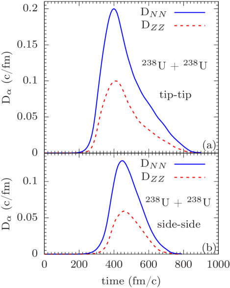
Figure 2: Neutron and proton diffusion coefficients as a function of time in the ${}^{238}\text{U}+{}^{238}\text{U}$ collisions at $E_{\text{c.m.}}=833$  MeV with the initial orbital angular momentum $\ell=300\hbar$ at tip-tip geometry (a) and side-side geometry (b).

Dispersions are determined from the solutions of the coupled differential equations (11-13) in which the diffusion coefficients provide source for development of the fluctuations. In addition to the diffusion coefficients, we also need to determine the derivatives of the drift coefficients with respect to the macroscopic variables $\left(N_{1},Z_{1}\right)$. In order to determine these derivatives, the Einstein’s relations in the over-damped limit provide a possible approach. According to the Einstein relation, drift coefficients are determine by the derivatives of the potential energy surface in the $\left(N,Z\right)$-plane,

$$v_{n}(t)= -\frac{D_{NN}}{T^{*}}\frac{\partial}{\partial N_{1}}U\left(N_{1},N_{1}\right)$$

$$v_{p}(t)= -\frac{D_{ZZ}}{T^{*}}\frac{\partial}{\partial Z_{1}}U\left(N_{1},Z_{1}\right),$$ (40)

where $T^{*}$ indicates effective temperature of the system. Because of the analytical structure, we can immediately take derivatives of the drift coefficients. Since ${}^{238}\text{U}+{}^{238}\text{U}$ is a symmetric system, the equilibrium state in the potential energy surface is located at the initial position with $N_{1}\to N_{0}=146$ and $Z_{1}\to Z_{0}=92.$ When fluctuations are not too far from the equilibrium point, we can parameterize the potential energy around the equilibrium in terms of two parabolic forms as given by Eq. (44) in the App. A Merchant and Nörenberg (1982). One of the parabolic forms extend along the bottom of the beta stability line, which is referred to as the iso-scalar path. The second parabolic form extends towards the perpendicular direction to the iso-scalar path, which is referred to as the iso-vector path. In order to specify the derivatives of the drift coefficients, we need to determine the reduced curvature parameters $\alpha$ and $\beta$ of these parabolic potential energy surfaces. Since the symmetric collisions do not exhibit drift in neutron or proton numbers, it is not possible to specify the reduced curvature parameters from the mean trajectory information of the symmetric collisions. As discussed in App. A, we can estimate the iso-vector curvature $\alpha$ parameter from the central collision of the neighboring ${}_{88}^{236}\text{Ra}_{148}+{}_{96}^{240}\text{Cm}_{144}$ system at at $E_{\text{c.m.}}=833$ MeV. As seen from the drift path of this system in Fig. 7, the system follows the iso-vector path closely and reaches the charge equilibrium rather rapidly during a time interval of $\Delta t\approx 150$ fm/c. The iso-vector drift path is suitable to estimate the average value of the iso-vector curvature parameters and we find $\alpha\approx 0.13$. After reaching the equilibrium in charge asymmetry rather rapidly, the system spends a long time in the vicinity of ${}^{238}\text{U}+{}^{238}\text{U}$ by following a curvy path due to complex quantal effect due to shell structure. Eventually, the system has a tendency to evolve toward asymmetry direction along the iso-scalar path, i.e along the beta stability line. It appears that the ${}^{238}\text{U}+{}^{238}\text{U}$ system is located at an unstable state on the beta stability line with a small and negative curvature parameter $\beta$ in the iso-scalar direction. It is not possible to provide reasonable estimation for this parameter from the drift path of the ${}_{88}^{236}\text{Ra}_{148}+{}_{96}^{240}\text{Cm}_{144}$ system in Fig. 8 beyond the equilibrium state at $(N_{1}=146,Z_{1}=92)$. With a negative curvature parameter in the iso-scalar direction, the system may exhibit broad diffusion along the beta stability line. In order obtain a reasonable value for $\beta$, we employ the cross-section data for production of gold isotopes from a previous investigation of the ${}^{238}\text{U}+{}^{238}\text{U}$ system at about the same energy Kratz et al. (2013). As discussed in Appendix B, we determine a small negative value of $\beta=-0.02$ for the reduced iso-scalar curvature parameter. Using these values for the reduced curvature parameters, we can determine the derivative of the drift coefficients as given in Eqs. (46)-(49) and calculate the neutron, the proton and the mixed dispersions from the solution of the differential Eqs. (32)-(34). As an example Fig. 3 shows the neutron, the proton and the mixed dispersions as a function of time in the ${}^{238}\text{U}+{}^{238}\text{U}$ collisions at $E_{\text{c.m.}}=833$ MeV with the initial orbital angular momentum $\ell=300\hbar$ at tip-tip geometry and side-side geometry. The asymptotic values of these dispersions for a range of the initial orbital angular momentum $\ell=(100-460)\hbar$ in tip-tip and side-side geometries are given in table 3.

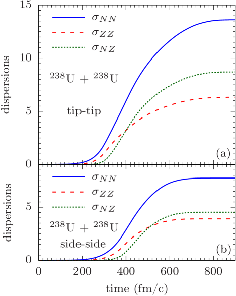
Figure 3: Neutron, proton and mixed variance as a function of time in the ${}^{238}\text{U}+{}^{238}\text{U}$ collisions at $E_{\text{c.m.}}=833$ MeV with the initial orbital angular momentum $\ell=300\hbar$ at tip-tip geometry (a) and side-side geometry (b).

Table 3: Asymptotic values of the neutron, the proton and the mixed dispersions in the ${}^{238}\text{U}+{}^{238}\text{U}$ collisions at $E_{\text{c.m.}}=833$ MeV with the range of orbital angular momentum $\ell=(100-460)\hbar$ at tip-tip geometry (left panel) and side-side geometry (right panel).

$\alpha=0.13\;\;\beta=-0.02\;\,$ (tip-tip)
$\ell_{i}(\hbar)$	$\sigma_{NN}$	$\sigma_{ZZ}$	$\sigma_{NZ}$	$\sigma_{AA}$
100	21.7	9.91	14.3	31.3
120	22.2	10.2	14.7	28.5
140	23.0	10.6	15.3	29.6
160	22.9	10.4	15.1	29.4
180	23.2	10.5	15.3	29.7
200	22.6	10.2	14.9	32.5
220	21.4	9.68	14.0	30.8
240	19.2	8.76	12.6	27.6
260	14.3	7.97	11.3	25.0
280	15.6	7.15	10.1	22.3
300	13.6	6.32	8.71	19.4
320	13.3	6.23	8.54	19.0
340	11.6	5.53	7.37	16.6
360	10.3	4.99	6.45	14.7
380	6.97	3.53	3.89	9.55
400	5.30	2.79	2.54	6.98
420	3.46	1.72	1.05	4.15
440	3.93	2.07	1.43	4.88
460	2.49	1.14	0.50	2.83

$\alpha=0.13\;\;\beta=-0.02\,$ (side-side)
$\ell_{i}(\hbar)$	$\sigma_{NN}$	$\sigma_{ZZ}$	$\sigma_{NZ}$	$\sigma_{AA}$
100	12.5	5.86	7.95	16.0
120	12.4	5.80	7.85	15.8
140	12.1	5.71	7.69	15.5
160	11.4	5.44	7.18	14.5
180	11.4	5.43	7.19	14.5
200	10.7	5.13	6.68	13.6
220	10.0	4.86	6.22	12.7
240	9.77	4.76	6.05	12.4
260	9.04	4.45	5.51	11.5
280	8.32	4.15	4.97	11.7
300	7.75	3.91	4.53	10.8
320	7.23	3.68	4.13	10.0
340	6.74	3.45	3.73	9.23
360	6.22	3.22	3.30	8.41
380	5.63	2.95	2.81	7.50
400	4.97	2.64	2.28	6.49
420	4.26	2.26	1.70	5.39
440	3.50	1.82	1.12	4.25
460	2.82	1.37	0.68	3.28

III.2 Cross-section of production of primary fragments

We calculate the cross-section for production of a primary fragment with neutron and proton numbers $(N,Z)$ using the standard expression,

$$\sigma(N,Z)=\frac{\pi\hbar^{2}}{2\mu E_{\text{c.m.}}}\sum_{\ell_{\min}}^{\ell_{\max}}(2\ell+1)P_{\ell}(N,Z).$$ (41)

Here, $P_{\ell}(N,Z)=\left(P_{\ell}^{t-t}(N,Z)+P_{\ell}^{s-s}(N,Z)\right)/2$ denotes the mean value of the probability of producing a primary fragment with neutron and proton numbers $(N,Z)$ in the tip-tip and the side-side collisions with the initial angular momentum $\ell$. These probabilities are presented in Eqs. (30)-(III.1) with the asymptotic values of dispersions given in Table 3 for tip-tip and side-side collisions. The mean values are equal to their initial values $\overline{N}=146$, $\overline{Z}=92$. The range of the summation over the initial angular momentum is taken as $\ell_{\min}=300$ and $\ell_{\max}=460$. This angular momentum range corresponds the experimental set up in which the detector is placed at an angular range $\theta=35^{\circ}\mp 5^{\circ}$ in the laboratory frame.

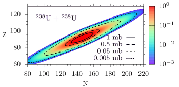
Figure 4: Double cross-sections $\sigma(N,Z)$ for production of primary fragments with neutron numbers N and proton numbers Z in (N,Z)-plane in the collisions of ${}^{238}\text{U}+{}^{238}\text{U}$ at $E_{\text{c.m.}}=833$ MeV. Elliptic lines indicate the set of isotopes with equal production cross-sections.

Fig. 4 shows the double cross-sections $\sigma(N,Z)$ in the $(N,Z)-$plane. We observe the cross-section distribution extends along the bottom of the beta stability and exhibits large dispersion in this direction as a result of the slight negative curvature of the potential energy along the iso-scalar direction. We note that the nucleon diffusion along the beta stability line is rather sensitive to the magnitude of the reduced iso-scalar curvature parameter $\beta$. Decreasing the magnitude of this parameter, the dispersion of the double cross-section along the beta stability direction is reduced. The cross-sections $\sigma(A)$ as a function of the mass numbers of the primary fragments are given by,

$$\sigma(A)=\frac{\pi\hbar^{2}}{2\mu E_{\text{c.m.}}}\sum_{\ell_{\min}}^{\ell_{\max}}(2\ell+1)P_{\ell}(A).$$ (42)

Here $P_{\ell}(A)=\left(P_{\ell}^{t-t}(A)+P_{\ell}^{s-s}(A)\right)/2$ denotes the mean value of the probability of producing a primary fragment with mass numbers $A$ in the tip-tip and the side-side collisions with the initial angular momentum $\ell$. These probabilities are determined by a simple Gaussian functions,

$$P(A)=\frac{1}{\sigma_{AA}\sqrt{2\pi}}\exp\left[-\frac{1}{2}\left(\frac{A-\overline{A}}{\sigma_{AA}}\right)^{2}\right],$$ (43)

where the mass dispersion is determined by $\sigma_{AA}^{2}=\sigma_{NN}^{2}+\sigma_{ZZ}^{2}+2\sigma_{NZ}^{2}$ and the mean mass number as $\overline{A}=238$. Fig. 5 shows the cross-sections as a function of the mass numbers of the primary fragments in the tip-tip and the side-side geometries and their mean values. We can calculate the cross-sections $\sigma(Z)$ of production of the primary fragments as a function of the atomic number using an expression similar to Eq. (42) by employing the Gaussian probability with the dispersion and the mean values as given by $\sigma_{ZZ}(Z)$ and $\overline{Z}=92$, respectively. Figure 6 shows the cross-sections as a function of the atomic numbers of the primary fragments in the tip-tip and the side-side geometries and their mean values.

Figure 5: Cross-sections $\sigma(A)$ for production of primary fragments as a function of mass number in the collisions of ${}^{238}\text{U}+{}^{238}\text{U}$ at $E_{\text{c.m.}}=833$ MeV in tip-tip, side-side geometries and mean values by dashed, dotted and solid blue lines, respectively.

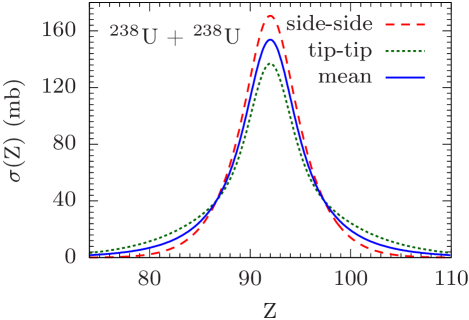
Figure 6: Cross-sections $\sigma(Z)$ for production of primary fragments as a function of mass number in the collisions of ${}^{238}\text{U}+{}^{238}\text{U}$ at $E_{\text{c.m.}}=833$ MeV in tip-tip, side-side geometries and mean values by dashed, dotted and solid blue lines, respectively.

IV CONCLUSIONS

We have carried out an investigation of mass and charge distributions of the primary fragments produced in the collisions of the ${}^{238}\text{U}+{}^{238}\text{U}$ system at $E_{\text{c.m.}}=833$ MeV. We calculate the probability distributions of the primary fragments by employing the quantal diffusion description. In the quantal diffusion approach, the concepts of the transport theory are merged with the mean-field description of the TDHF with the help of the SMF approach. It is then possible to express the diffusion coefficients of the relevant macroscopic variables in terms of the occupied single-particle wave functions of the TDHF. Since the Langevin equations of the macroscopic variables are equivalent to the Fokker- Planck description for the distribution of the macroscopic variables, under certain conditions, it is possible give nearly analytical description for the distribution functions of the macroscopic variables and the cross-sections. In the calculations of the cross-sections of production of the primary fragment for each initial angular momentum or equivalently for each impact parameter, we need to determine the mean values of the neutron and proton numbers of the fragments and the neutron, the proton and the mixed dispersions of the distribution functions. The mean values are determined by the TDHF descriptions. The variances are calculated from the solutions of three coupled differential equations in which diffusion coefficients of neutron and protons act as the source terms. The behavior of the potential energy surface of the di-nuclear complex makes an important effect on the neutron and proton diffusion mechanism. It is possible to determine the curvature parameters of the potential energy in the collisions of asymmetric systems from the drift information with the help of the Einstein’s relation in the over-damped limit. Since collisions of the symmetric systems, such as the collisions of ${}^{238}\text{U}+{}^{238}\text{U}$, do not exhibit drift of the neutron and proton degrees of freedom, we need to employ other methods to specify the curvature parameters of the potential energy. In this work, we employ the central collision of a neighboring system ${}^{236}\text{Ra}+{}^{240}\text{Cm}$ at the same bombarding energy. The system initially drifts nearly along the iso-vector direction and reach the charge equilibrium state rather rapidly. From the iso-vector drift information, we can estimate the reduced curvature parameter of the potential energy as $\alpha=0.13$. After reaching the charge equilibration, the system spends a long time in the vicinity of ${}^{238}\text{U}+{}^{238}\text{U}$ state and eventually has a tendency drift along the iso-scalar path away from the symmetric state. This behavior indicates the symmetric ${}^{238}\text{U}+{}^{238}\text{U}$ is located at an unstable equilibrium position with a small negative curvature toward the iso-scalar direction. However, from the drift information it is not possible to estimate the iso-scalar reduced curvature parameter $\beta$. Since the negative curvature may lead to broad diffusion along the beta stability line, it is important to determine this curvature parameter accurately. Therefore, we regard the reduced curvature in the iso-scalar direction as a parameter and estimate its value with the help of the isotopic cross-section data of gold nucleus from a previous investigation of the ${}^{238}\text{U}+{}^{238}\text{U}$ collisions at about the same energy. In this work, we present calculations for production of the primary fragments with the curvature parameters $\alpha=0.13$ and $\beta=-0.02$. The primary fragments are excited and cool dawn by the de-excitation processes of particle emission, mostly neutrons and by sequential fission of the heavy fragments. Calculations of the secondary cross-sections exceed the scope of the present work. We plan to investigate the de-excitation process of the primary fragments in the collisions of ${}^{238}\text{U}+{}^{238}\text{U}$ and calculate the secondary cross-sections in a subsequent study.

Appendix A CURVATURE PARAMETERS OF THE POTENTIAL ENERGY

The charge asymmetry of uranium ${}_{92}^{238}\text{U}_{146}$ is $(146-92)/(146+92)=0.227$. The dashed green line in Fig. 7 represents the nuclei with nearly equal charge asymmetry $(N-Z)/(N+Z)=0.22-0.23$. We refer to this line as the iso-scalar line which extends nearly parallel to the lower part of the beta stability valley in this region. We refer to the dashed red line as the iso-vector line which is perpendicular to the iso-scalar path. We parameterize the potential energy surface in the vicinity of the equilibrium $(N_{0}=146,Z_{0}=92)$ in terms of two parabolic forms along the iso-scalar and iso-vector paths as,

$$U(N_{1},Z_{1})=\frac{1}{2}aR_{S}^{2}(N_{1},Z_{1})+\frac{1}{2}bR_{V}^{2}(N_{1},Z_{1}).$$ (44)

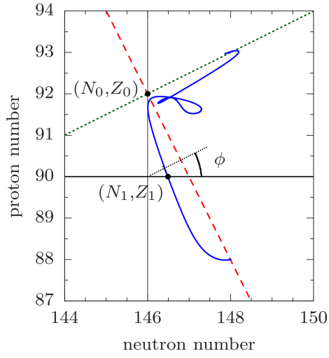
Figure 7: Drift path of the radium-like fragments in the central collisions of the ${}^{236}\text{Ra}+{}^{240}\text{Cm}$ system at $E_{\text{c.m.}}=833$ MeV (solid blue line) at tip-tip geometry. Dashed green line starting at $(Z_{1}=92,N_{1}=144)$ and the perpendicular dashed red line are the iso-scalar and iso-vector paths, respectively.

The vertical distances $R_{S}$ and $R_{V}$ of a point ($N_{1},Z_{1}$) representing a fragment from the iso-scalar and the iso-vector lines, respectively are given by,

$$R_{S}= (Z_{0}-Z_{1})\cos\phi+(N_{1}-N_{0})\sin\phi,$$

$$R_{V}= (Z_{0}-Z_{1})\sin\phi-(N_{1}-N_{0})\cos\phi.$$ (45)

According to the Einstein relation in the over-damped limit neutron and proton drift coefficients are related to the driving potential as,

$$v_{n}=-\frac{D_{NN}}{T}\frac{\partial U}{\partial N_{1}}=-\alpha D_{NN}R_{S}\sin\phi+\beta D_{NN}R_{V}\cos\phi$$

$$v_{z}=-\frac{D_{ZZ}}{T}\frac{\partial U}{\partial Z_{1}}=+\alpha D_{ZZ}R_{S}\cos\phi+\beta D_{ZZ}R_{V}\sin\phi\;.$$

Here, the temperature is absorbed in the reduced curvature parameters as $\alpha=a/T$ and $\beta=b/T$. Because of the analytical form, we can readily calculate the derivatives of the drift coefficients to obtain,

$$\partial v_{n}(t)/\partial N_{1}=-D_{NN}\left(\beta\cos^{2}\phi+\alpha\sin^{2}\phi\right)$$ (46)

$$\partial v_{n}(t)/\partial Z_{1}=+D_{NN}\left(\alpha-\beta\right)\cos\phi\sin\phi$$ (47)

$$\partial v_{p}(t)/\partial Z_{1}=-D_{ZZ}\left(\beta\sin^{2}\phi+\alpha\cos^{2}\phi\right)$$ (48)

$$\partial v_{p}(t)/\partial N_{1}=+D_{ZZ}\left(\alpha-\beta\right)\cos\phi\sin\phi\;.$$ (49)

The reduced curvature parameters are determined by the drift and the diffusion coefficients as,

$$\alpha R_{S}(t)=\frac{v_{z}(t)}{D_{ZZ}(t)}\cos\phi-\frac{v_{n}(t)}{D_{NN}(t)}\sin\phi$$ (50)

and

$$\beta R_{V}(t)=\frac{v_{z}(t)}{D_{ZZ}(t)}\sin\phi+\frac{v_{n}(t)}{D_{NN}(t)}\cos\phi\;.$$ (51)

In collisions of symmetric systems, the drift coefficients vanish and the mean values of the neutron and proton numbers of the fragments are equal to the equilibrium values of the colliding nuclei $\overline{N}_{1}=N_{0}$, $\overline{Z}_{1}=Z_{0}$. As a result, it is not possible to determine the reduced curvature parameters from the Eq. (50) and Eq. (51).

In order to estimate the reduced curvature parameters, we consider the central collision of a neighboring system of ${}_{88}^{236}\text{Ra}_{148}+{}_{96}^{240}\text{Cm}_{144}$ at the same bombarding energy $E_{\text{c.m.}}=833$ MeV. We consider ${}^{236}\text{Ra}$ as the projectile. Figure 8 shows the neutron mumber ${N}_{1}(t)$ and the proton number ${Z}_{1}(t)$ as a function of time. Blue line in Fig. 7 shows the drift path of the projectile-like fragments in the $(N,Z)$-plane. We observe that the system rapidly evolves toward the equilibrium charge asymmetry of the ${}^{238}\text{U}+{}^{238}\text{U}$ system nearly along the iso-vector direction from the initial state at point A toward the state at point B. This segment of the drift path is suitable to determine the average value of the reduced iso-vector curvature as,

$$\alpha\int_{t_{A}}^{t_{B}}dt\left[R_{S}(t)\right]=\int_{t_{A}}^{t_{B}}dt\left[\frac{v_{z}(t)}{D_{ZZ}(t)}\cos\phi-\frac{v_{n}(t)}{D_{NN}(t)}\sin\phi\right]$$ (52)

where $t_{A}=250$ fm/c and $t_{B}=400$ fm/c as indicated in Fig. 8. We find the reduced iso-vector curvature parameter as $\alpha=0.13$. In Fig. 7, after the symmetric state ${}^{238}\text{U}+{}^{238}\text{U}$, because of quantal effects due to shell structure, the TDHF drift path follows a complex pattern for a long time and subsequently appears to drift toward asymmetry along the iso-scalar direction. This behavior indicates that the symmetric state is an unstable equilibrium point in the iso-scalar direction, i.e. along the beta stability line, and the average potential energy has an inverted parabolic shape with a negative curvature parameter. Such potential shape may lead to relative large diffusion along the beta stability direction. Unfortunately, the drift segment after the symmetric state until the time which the fragment separates is not suitable to estimate the average value of the reduced iso-scalar curvature parameter $\beta$.

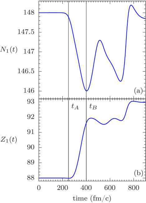
Figure 8: Neutron $N_{1}(t)$ and proton $Z_{1}(t)$ numbers of radium-like fragments as function of time in the central collisions of the ${}^{236}\text{Ra}+{}^{240}\text{Cm}$ system at $E_{\text{c.m.}}=833$ MeV .(solid blue line) at tip-tip geometry.

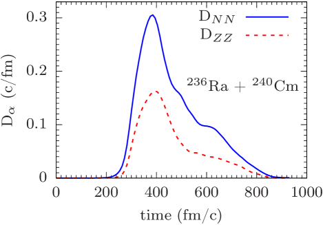
Figure 9: Neutron and proton diffusion coefficients as function of time in the central collisions of the ${}^{236}\text{Ra}+{}^{240}\text{Cm}$ system at $E_{\text{c.m.}}=833$ MeV at tip-tip geometry.

Appendix B CURVATURE PARAMETERS ALONG THE BETA STABILITY

We consider the reduced iso-scalar curvature $\beta$ as a parameter. In order obtain a reasonable value for $\beta$, we employ the cross-section data for production of gold isotopes from a previous investigation of the ${}^{238}\text{U}+{}^{238}\text{U}$ system at about the same energy. We calculate the distribution of the cross-sections $\sigma(N=A-Z,Z)$ primary gold isotopes with the atomic number $Z=79$ and mass numbers $A$ using Eq. (41) for the double $\sigma(N,Z)$ cross-sections. In order to cover the angular range of the experimental set up in Ref. Kratz et al. (2013), the range of the angular momentum summation in Eq. (41) is taken as $\ell_{\min}=100$ and $\ell_{\max}=460$. Fig. 10 shows the cross-sections for production of the primary gold isotopes which are calculated with the reduced iso-vector curvature $\alpha=0.13$ and the reduced iso-scalar curvature $\beta=-0.02$. The primary gold isotopes are excited and cool down mainly by neutron emissions. In determining the average number of the emitted neutrons, we need to estimate the average excitation energy of these isotopes. The TDHF calculations presented in Table 1 and Table 2, do not give accurate information for the total kinetic energy loss (TKEL) in these channels. However for a rough estimate we can take the results for the initial angular momentum $L=300\hbar$, which is about the waited mean value of the angular momentum range. For this angular momentum, the TKEL in the tip-tip and the side-side geometries are $217$ MeV and $135$ MeV, respectively. For the gold channel U+U $\rightarrow$ Au(195,79)+Db(281,105) the $Q_{gg}-$value is 24.1 MeV. Sharing the TKEL and the $Q_{gg}-$value in proportion to the masses, we find the average excitation energy of the gold isotopes to be $86.8$ MeV and $54.0$ MeV, in the tip-tip and the side-side geometries, respectively. Assuming one neutron emitted per $10.0$ MeV, on the average about $9$, $5$ and $7$ neutrons are emitted in the tip-tip, in the side-side and in the mean geometry, respectively. In Fig. 10, if we shift the mean gold isotope distribution by 7 units to the left, the peak value of the cross-sections matches the peak value of the gold data. This indicates $\beta=-0.02$ is a reasonable estimate for the reduced curvature parameter in the iso-scalar direction. We note that the calculations overestimate the isotopic width, which most probably is due to the parabolic approximation of the potential energy.

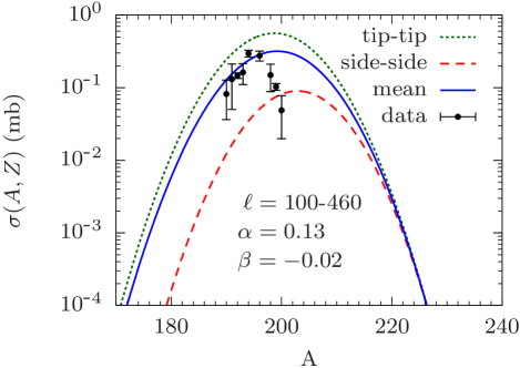
Figure 10: Cross-section of gold $Z=79$ isotopes averaged over tip-tip and side-side geometries as a function of the mass$A$numbers in the collisions of ${}^{238}\text{U}+{}^{238}\text{U}$ system at $E_{\text{c.m.}}=833$ MeV calculated with curvature parameters $\alpha=0.13$ and $\beta=-0.02$. Solid dots indicate data taken from Kratz et al. (2013).

References

- Adamian et al. (2003) G. G. Adamian, N. V. Antonenko, and W. Scheid, “Characteristics of quasifission products within the dinuclear system model,” Phys. Rev. C 68, 034601 (2003).
- Valery Zagrebaev and Walter Greiner (2007) Valery Zagrebaev and Walter Greiner, “Shell effects in damped collisions: a new way to superheavies,” J. Phys. G 34, 2265 (2007).
- Aritomo (2009) Y. Aritomo, “Analysis of dynamical processes using the mass distribution of fission fragments in heavy-ion reactions,” Phys. Rev. C 80, 064604 (2009).
- Adamian et al. (2010) G. G. Adamian, N. V. Antonenko, V. V. Sargsyan, and W. Scheid, “Possibility of production of neutron-rich Zn and Ge isotopes in multinucleon transfer reactions at low energies,” Phys. Rev. C 81, 024604 (2010).
- Barrett et al. (2015) J. S. Barrett, W. Loveland, R. Yanez, S. Zhu, A. D. Ayangeakaa, M. P. Carpenter, J. P. Greene, R. V. F. Janssens, T. Lauritsen, E. A. McCutchan, A. A. Sonzogni, C. J. Chiara, J. L. Harker, and W. B. Walters, “ reaction: A test of models of multinucleon transfer reactions,” Phys. Rev. C 91, 064615 (2015).
- Devaraja et al. (2015) H. M. Devaraja, S. Heinz, O. Beliuskina, V. Comas, S. Hofmann, C. Hornung, G. Münzenberg, K. Nishio, D. Ackermann, Y. K. Gambhir, M. Gupta, R. A. Henderson, F. P. Heßberger, J. Khuyagbaatar, B. Kindler, B. Lommel, K. J. Moody, J. Maurer, R. Mann, A. G. Popeko, D. A. Shaughnessy, M. A. Stoyer, and A. V. Yeremin, “Observation of new neutron-deficient isotopes with Z92 in multinucleon transfer reactions,” Phys. Lett. B 748, 199–203 (2015).
- Zhao et al. (2016) Kai Zhao, Zhuxia Li, Yingxun Zhang, Ning Wang, Qingfeng Li, Caiwan Shen, Yongjia Wang, and Xizhen Wu, “Production of unknown neutron–rich isotopes in collisions at near–barrier energy,” Phys. Rev. C 94, 024601 (2016).
- Sekizawa and Yabana (2016) Kazuyuki Sekizawa and Kazuhiro Yabana, “Time-dependent Hartree-Fock calculations for multinucleon transfer and quasifission processes in the reaction,” Phys. Rev. C 93, 054616 (2016).
- Feng (2017) Zhao-Qing Feng, “Production of neutron–rich isotopes around in multinucleon transfer reactions,” Phys. Rev. C 95, 024615 (2017).
- Sekizawa (2017) Kazuyuki Sekizawa, “Enhanced nucleon transfer in tip collisions of ,” Phys. Rev. C 96, 041601(R) (2017).
- Kazuyuki Sekizawa (2019) Kazuyuki Sekizawa, “TDHF Theory and Its Extensions for the Multinucleon Transfer Reaction: A Mini Review,” Front. Phys. 7, 20 (2019).
- Mun et al. (2019) Myeong-Hwan Mun, Kyujin Kwak, G. G. Adamian, and N. V. Antonenko, “Possible production of neutron-rich Md isotopes in multinucleon transfer reactions with Cf and Es targets,” Phys. Rev. C 99, 054627 (2019).
- Saiko and Karpov (2019) V. V. Saiko and A. V. Karpov, “Analysis of multinucleon transfer reactions with spherical and statically deformed nuclei using a Langevin-type approach,” Phys. Rev. C 99, 014613 (2019).
- Jiang and Wang (2020) Xiang Jiang and Nan Wang, “Probing the production mechanism of neutron-rich nuclei in multinucleon transfer reactions,” Phys. Rev. C 101, 014604 (2020).
- Kozulin et al. (2012) E. M. Kozulin, E. Vardaci, G. N. Knyazheva, A. A. Bogachev, S. N. Dmitriev, I. M. Itkis, M. G. Itkis, A. G. Knyazev, T. A. Loktev, K. V. Novikov, E. A. Razinkov, O. V. Rudakov, S. V. Smirnov, W. Trzaska, and V. I. Zagrebaev, “Mass distributions of the system at laboratory energies around the Coulomb barrier: A candidate reaction for the production of neutron–rich nuclei at N=126,” Phys. Rev. C 86, 044611 (2012).
- Kratz et al. (2013) J. V. Kratz, M. Schädel, and H. W. Gäggeler, “Reexamining the heavy-ion reactions and and actinide production close to the barrier,” Phys. Rev. C 88, 054615 (2013).
- Watanabe et al. (2015) Y. X. Watanabe, Y. H. Kim, S. C. Jeong, Y. Hirayama, N. Imai, H. Ishiyama, H. S. Jung, H. Miyatake, S. Choi, J. S. Song, E. Clement, G. de France, A. Navin, M. Rejmund, C. Schmitt, G. Pollarolo, L. Corradi, E. Fioretto, D. Montanari, M. Niikura, D. Suzuki, H. Nishibata, and J. Takatsu, “Pathway for the Production of Neutron–Rich Isotopes around the Shell Closure,” Phys. Rev. Lett. 115, 172503 (2015).
- Desai et al. (2019) V. V. Desai, W. Loveland, K. McCaleb, R. Yanez, G. Lane, S. S. Hota, M. W. Reed, H. Watanabe, S. Zhu, K. Auranen, A. D. Ayangeakaa, M. P. Carpenter, J. P. Greene, F. G. Kondev, D. Seweryniak, R. V. F. Janssens, and P. A. Copp, “The reaction: A test of models of multi-nucleon transfer reactions,” Phys. Rev. C 99, 044604 (2019).
- Valery Zagrebaev and Walter Greiner (2008) Valery Zagrebaev and Walter Greiner, “Production of New Heavy Isotopes in Low–Energy Multinucleon Transfer Reactions,” Phys. Rev. Lett. 101, 122701 (2008).
- Zagrebaev and Greiner (2011) V. I. Zagrebaev and Walter Greiner, “Production of heavy and superheavy neutron-rich nuclei in transfer reactions,” Phys. Rev. C 83, 044618 (2011).
- Zagrebaev et al. (2012) V. I. Zagrebaev, A. V. Karpov, and Walter Greiner, “Possibilities for synthesis of new isotopes of superheavy elements in fusion reactions,” Phys. Rev. C 85, 014608 (2012).
- Karpov and Saiko (2017) A. V. Karpov and V. V. Saiko, “Modeling near-barrier collisions of heavy ions based on a Langevin-type approach,” Phys. Rev. C 96, 024618 (2017).
- Simenel (2012) Cédric Simenel, “Nuclear quantum many-body dynamics,” Eur. Phys. J. A 48, 152 (2012).
- Nakatsukasa et al. (2016) Takashi Nakatsukasa, Kenichi Matsuyanagi, Masayuki Matsuo, and Kazuhiro Yabana, “Time-dependent density-functional description of nuclear dynamics,” Rev. Mod. Phys. 88, 045004 (2016).
- Oberacker et al. (2014) V. E. Oberacker, A. S. Umar, and C. Simenel, “Dissipative dynamics in quasifission,” Phys. Rev. C 90, 054605 (2014).
- Oberacker et al. (2010) V. E. Oberacker, A. S. Umar, J. A. Maruhn, and P.–G. Reinhard, “Microscopic study of the reactions: Dynamic excitation energy, energy-dependent heavy-ion potential, and capture cross section,” Phys. Rev. C 82, 034603 (2010).
- Umar et al. (2015) A. S. Umar, V. E. Oberacker, and C. Simenel, “Shape evolution and collective dynamics of quasifission in the time-dependent Hartree-Fock approach,” Phys. Rev. C 92, 024621 (2015).
- Simenel and Umar (2018) C. Simenel and A. S. Umar, “Heavy-ion collisions and fission dynamics with the time–dependent Hartree-Fock theory and its extensions,” Prog. Part. Nucl. Phys. 103, 19–66 (2018).
- Simenel (2010) Cédric Simenel, “Particle Transfer Reactions with the Time-Dependent Hartree-Fock Theory Using a Particle Number Projection Technique,” Phys. Rev. Lett. 105, 192701 (2010).
- Roger Balian and Marcel Vénéroni (1984) Roger Balian and Marcel Vénéroni, “Fluctuations in a time-dependent mean-field approach,” Phys. Lett. B 136, 301–306 (1984).
- Balian and Vénéroni (1985) R. Balian and M. Vénéroni, “Time-dependent variational principle for the expectation value of an observable: Mean-field applications,” Ann. Phys. 164, 334 (1985).
- Broomfield and Stevenson (2008) J. M. A. Broomfield and P. D. Stevenson, “Mass dispersions from giant dipole resonances using the Balian-Vénéroni variational approach,” J. Phys. G 35, 095102 (2008).
- Williams et al. (2018) E. Williams, K. Sekizawa, D. J. Hinde, C. Simenel, M. Dasgupta, I. P. Carter, K. J. Cook, D. Y. Jeung, S. D. McNeil, C. S. Palshetkar, D. C. Rafferty, K. Ramachandran, and A. Wakhle, “Exploring Zeptosecond Quantum Equilibration Dynamics: From Deep-Inelastic to Fusion-Fission Outcomes in Reactions,” Phys. Rev. Lett. 120, 022501 (2018).
- Godbey and Umar (2020) Kyle Godbey and A. S. Umar, “Quasifission Dynamics in Microscopic Theories,” Front. Phys. 8, 40 (2020).
- Ayik (2008) S. Ayik, “A stochastic mean-field approach for nuclear dynamics,” Phys. Lett. B 658, 174 (2008).
- Lacroix and Ayik (2014) Denis Lacroix and Sakir Ayik, “Stochastic quantum dynamics beyond mean field,” Eur. Phys. J. A 50, 95 (2014).
- Gardiner (1991) C. W. Gardiner, Quantum Noise (Springer–Verlag, Berlin, 1991).
- Weiss (1999) U. Weiss, Quantum Dissipative Systems, 2nd ed. (World Scientific, Singapore, 1999).
- Ayik et al. (2017) S. Ayik, B. Yilmaz, O. Yilmaz, A. S. Umar, and G. Turan, “Multinucleon transfer in central collisions of ,” Phys. Rev. C 96, 024611 (2017).
- Ayik et al. (2018) S. Ayik, B. Yilmaz, O. Yilmaz, and A. S. Umar, “Quantal diffusion description of multinucleon transfers in heavy–ion collisions,” Phys. Rev. C 97, 054618 (2018).
- Yilmaz et al. (2018) B. Yilmaz, S. Ayik, O. Yilmaz, and A. S. Umar, “Multinucleon transfer in and in a stochastic mean-field approach,” Phys. Rev. C 98, 034604 (2018).
- Ayik et al. (2019) S. Ayik, B. Yilmaz, O. Yilmaz, and A. S. Umar, “Quantal diffusion approach for multinucleon transfers in XePb collisions,” Phys. Rev. C 100, 014609 (2019).
- Sekizawa and Ayik (2020) Kazuyuki Sekizawa and Sakir Ayik, “Quantal diffusion approach for multinucleon transfer processes in the reactions: Towards the production of unknown neutron-rich nuclei,” (2020), arXiv:2003.07786 [nucl-th] .
- Yilmaz et al. (2020) O. Yilmaz, G. Turan, and B. Yilmaz, “Quasi-fission and fusion-fission reactions in collisions at MeV,” Eur. Phys. J. A 56, 37 (2020).
- Umar et al. (1991) A. S. Umar, M. R. Strayer, J. S. Wu, D. J. Dean, and M. C. Güçlü, “Nuclear Hartree-Fock calculations with splines,” Phys. Rev. C 44, 2512–2521 (1991).
- Umar and Oberacker (2006) A. S. Umar and V. E. Oberacker, “Three-dimensional unrestricted time-dependent Hartree-Fock fusion calculations using the full Skyrme interaction,” Phys. Rev. C 73, 054607 (2006).
- Ka–Hae Kim et al. (1997) Ka–Hae Kim, Takaharu Otsuka, and Paul Bonche, “Three-dimensional TDHF calculations for reactions of unstable nuclei,” J. Phys. G 23, 1267 (1997).
- Hannes Risken and Till Frank (1996) Hannes Risken and Till Frank, The Fokker–Planck Equation (Springer–Verlag, Berlin, 1996).
- Schröder et al. (1981) W. U. Schröder, J. R. Huizenga, and J. Randrup, “Correlated mass and charge transport induced by statistical nucleon exchange in damped nuclear reactions,” Phys. Lett. B 98, 355–359 (1981).
- Merchant and Nörenberg (1982) A. C. Merchant and W. Nörenberg, “Microscopic transport theory of heavy-ion collisions,” Z. Phys. A 308, 315–327 (1982).