Nitsche’s Method for resolving boundary conditions on embedded interfaces using XFEM in Code Aster

Master of Science Thesis
Ecole Centrale de Nantes
Nitsche’s Method for resolving boundary conditions on embedded interfaces using XFEM in Code Aster

Abstract

As X-FEM approximation doesn’t need meshing of the crack, the method has garnered a lot of attention from industrial point of view. This thesis report summarises some of the concepts involved in Nitsche’s approach for resolving boundary conditions in embedded interfaces using XFEM. We consider here cases in which the jump of a field across the interface is given, as well as cases in which the primary field on the interface is given. We will first derive the basics of Nitsche’s method and then discretize it with X-FEM using shifted basis enrichment. We will then implement this on an open source platform, Code-Aster.

Nanda Gopala Kilingar

Submitted in fulfillment of the requirements for the degree of
Master of Science in Computational Mechanics

*Nitsche’s Method for resolving boundary conditions on embedded interfaces using XFEM in Code Aster

Supervisors: Patrick Massin, Director, IMSIA, EDF R&D Paris-Saclay

Alexandre Martin, Research Engineer, IMSIA CNRS

Acknowledgments

I would like to thank Parick Massin for providing me the opportunity to conduct an internship at EDF R&D and his constant guidance during my time working in a state-of-art facility with the best infrastructure possible. I thank Alexandre Martin for his supervision and his inputs that led me to the successful completion of the internship. I would like to thank Marcel Ndeffo for his help with various parts of the subject and also my fellow interns and colleagues of IMSIA at EDF R&D.

I would like to thank my professors and lecturers at Ecole Centrale Nantes for all the knowledge they provided in the preceding semesters that led me to undergo this internship. Last, but not the least, I would like to express my gratitude to ECN for giving me an opportunity to pursue my master’s studies and providing a platform for me to expand my scope of understanding.

Contents

1. 1 Presentation
   1. 1.1 EDF R&D
   2. 1.2 IMSIA
   3. 1.3 Code Aster
   4. 1.4 Salome Meca
   5. 1.5 ASTK
2. 2 Introduction to the Work
   1. 2.1 Nitsche’s Approach on General boundary condition
   2. 2.2 Comparison with other approaches
   3. 2.3 Application to Interfaces
3. 3 Nitsche’s method with Elastostatic (Cauchy Navier) Equations
   1. 3.1 Discretization of the problem
      1. 3.1.1 Jump Condition
      2. 3.1.2 Dirichlet condition
   2. 3.2 Discretization with a shifted basis enrichment
      1. 3.2.1 Jump Condition
      2. 3.2.2 Dirichlet Condition
   3. 3.3 Non-Linear Iteration
      1. 3.3.1 Jump conditions
      2. 3.3.2 Dirichlet Conditions
   4. 3.4 Weighted Discretization
4. 4 Analytical Solution of a simple problem
   1. 4.1 Exact numerical solution
   2. 4.2 Discretized solution
      1. 4.2.1 Jump in Displacement type solution
      2. 4.2.2 Dirichlet type solution
5. 5 Implementation in Code-Aster
   1. 5.1 Options and routines
   2. 5.2 Simple test case
   3. 5.3 Circular Inclusion problem
6. 6 Conclusion and future scope
7. ‣ Nitsche’s Method for resolving boundary conditions on embedded interfaces using XFEM in Code Aster
8. A Stabilization parameter
9. ‣ Appendix

List of Figures

1. 1.1 GUI of Salome Meca 7.8.0 displaying a 2D surface with mesh during postprocessing
2. 1.2 ASTK GUI letting the user select the mesh file and the output file along with the command file
3. 2.1 Notation for two-sided problem
4. 4.1 simple problem
5. 4.2 simple problem discretized
6. 5.1 Rectangular block of size $5\times 5\times 25$ with a plane interface at $z=12.5$
7. 5.2 the solution as obtained in Code Aster after analyzing a problem of jump type using non-linear Newton iterations.
8. 5.3 Relative energy norm error for Dirichlet conditions and the study of their variation with change in stabilization parameter in Nitsche’s and penalization methods.
9. 5.4 Relative energy norm error for Jump conditions and the study of their variation with change in stabilization parameter in Nitsche’s and penalization methods.
10. 5.5 Relative L2 norm error for Dirichlet conditions and the study of their variation with change in stabilization parameter in Nitsche’s and penalization methods.
11. 5.6 Relative L2 norm error for Jump conditions and the study of their variation with change in stabilization parameter in Nitsche’s and penalization methods.
12. 5.7 Problem statement of the circular inclusion problem (the gray area is the numerical domain)
13. 5.8 Circular inclusion problem solution on an irregular grid of size $h=0.2$. Notice how the element is divided into subelements at the interface.
14. 5.9 Circular inclusion problem solution on an irregular grid of size $h=0.0125$. In this close up view the effect of level set on the mesh and the solution can be seen.
15. 5.10 Circular inclusion problem solution on an regular grid of size $h=0.05$. The enrichment is extended to an element beyond the interface in both sides.
16. 5.11 Circular inclusion problem solution on an regular grid of size $h=0.0125$. Magnitude of the displacement solution on the entire domain and its variation with respect to x and y direction.
17. 5.12 Circular inclusion problem solution on an regular grid of size $h=0.0125$. Solution of the discontinuous stresses in the domain
18. 5.13 Relative energy norm error for the circular inclusion problem - comparison with various grids and order of the shape functions.
19. 5.14 Relative L2 norm error for the circular inclusion problem - comparison with various grids and order of the shape functions.
20. 5.15 Relative energy norm error for the circular inclusion problem - comparison between the three methods on a regular quadratic grid.
21. 5.16 Relative L2 norm error for the circular inclusion problem - comparison between the three methods on a regular quadratic grid.
22. 5.17 Condition number comparison for the circular inclusion problem between Nitsche’s method and penalty method.

List of Tables

1. 1 Term by term comparison of the variational form of ’Jump’ and ’Dirichlet’ problems
2. 2 Term by term comparison of the variational form of ’Jump’ and ’Dirichlet’ interfacial displacement problems

1 Presentation

1.1 EDF R&D

As the leading global electricity provider, EDF operates in every energy business line, from generation to customer offer, from transmission to distribution and from research to innovation. With sales of upto €73 billion, about 55% of it comes from France while the rest is generated by international sales and other activities. Generating about 623.5TWh with around 76.6% of it coming from nuclear sources, EDF is almost 87% $\mbox{CO}_{2}$ free. It invests about €650 million research and development alone.[13]

Strategy

As today’s increasingly digital world dramatically changes the way we produce and consume, research into electricity generation, transmission and consumption is of decisive importance. To succeed in the energy transition, the 2,100 EDF’s R&D division staff (representing 29 nationalities) are currently working on many different projects designed simultaneously to deliver low-carbon power generation, smarter energy transmission grids and more responsible energy consumption. The missions of EDF’s R&D are structured around 3 key priorities.[14]

Priority

1: consolidating and developing competitive, low-carbon energy generation mixes: One of the major challenges presented by the energy transition is to ensure the efficient coexistence of traditional generating methods – particularly in terms of improving nuclear plant safety, efficiency and operating life even further – with the development of renewables.

Priority

2: developing new energy services for customers: Responding to customer expectations means thinking about new solutions that respond effectively to variable energy demand while also limiting carbon emissions. This involves:

• promoting new ways of using electricity more efficiently (heat pumps, electric mobility, etc.)

• developing digital energy services (real-time consumption control, smart load balancing, etc.)

• developing solutions that encourage energy savings (insulation, appliances, etc.)

• supporting local authorities in their energy plans for sustainable cities and regions

Priority

3: preparing the electrical systems of tomorrow: This involves developing smart management tools that will make electrical systems more flexible and adaptable, encouraging the injection of intermittent energy sources into the grid, and designing new sustainable energy solutions at local and regional level.

1.2 IMSIA

The IMSIA, Institute of Mechanical Sciences and its Industrial Applications is a mixed EDF-CNRS research unit created in january 2004. The laboratory is part of the research facilities of EDF. Its human resources come from three thematic research departments of EDF R&D (Mechanical Analyses and Acoustics (AMA), Material and Mechanics of Components (MMC), Neutronic Simulation, Information Technology and Scientific Computation (SINETICS)). Mechanical resistance of structures confronted to ageing problems, under the constraints of maintained safety and economical performance, constitutes an important matter for a society facing decisive economic choices and requiring at the same time an improved safety with respect to industrial risks. In that perspective, increasing the lifetime of installations, following and validating maintenance repairs or structural modifications, monitoring their real behaviour with respect to design specifications and the need of in service lifetime monitoring, constitute the key issues that need to be associated to sustainable development and that require numerous multidisciplinary scientific progresses. These societal issues are shared with the Engineering Department of the CNRS and are beyond the sole preoccupations of EDF. The laboratory is devoted to three main research operations :

• Damage and rupture of structures (metallic and civil engineering ones) ;

• Data identification, assimilation, exploitation and reduction (loadings, material properties) and coupled problems involving structures ;

• Computational Mechanics : methods, formulations and algorithms for non linear structural calculations.

The IMSIA relies mainly on Code_Aster libre, free software under GNU General Public Licence. It contributes to its evolution in collaboration with the development team of the software at EDF R&D and its industrial an academic partners. The IMSIA is part of the Parisian Federation for Mechanics Fédération de Recherche Francilienne en Mécanique des Matériaux, Structures et Procédés (F2M2SP).

1.3 Code Aster

Code_Aster offers a full range of multiphysical analysis and modelling methods that go well beyond the standard functions of a thermomechanical calculation code: from seismic analysis to porous media via acoustics, fatigue, stochastic dynamics, etc. Its modelling, algorithms and solvers are constantly under construction to improve and complete them (1,200,000 lines of code, 200 operators). Resolutely open, it is linked, coupled and encapsulated in numerous ways.[16]

With the Code_Aster’s architecture, advanced users can easily work on the code, partly thanks to PYTHON, in order to write professional applications, introduce finite elements and constitutive laws or define new exchange formats. The Code_Aster user describes the parameters and progression of the survey in a command file. The grammar and vocabulary of this language, which is specific to Code_Aster and written in the PYTHON language, are described in catalogues. This structuring of the information makes it possible to enhance the language with new commands at lesser cost or to encapsulate recurring calculation sequences into macrocommands. A more advanced use enables users to introduce programming in their datasets: from basic ones (check structures, loop and tests) to more complex ones using all the richness of PYTHON (methods, classes, importing graphics or mathematical calculation modules, etc.) Here is a first basic example: Optimising a pipe bendradius. Any calculation result can be uploaded in the PYTHON space. Here we use an indicator for maximal stress in the elbow in order to repeat the mesh, calculation and postprocessing tasks, thus optimizing the pipe bend-radius. Another example: with the MEIDEE macro-command, it is possible to launch calculations for stress identification on wire structure. Using graphics modules provides an intuitive interface that helps proceeding to the identification. By encapsulating it into a macro-command it becomes a professional tool that make the methodology reliable and durable.

1.4 Salome Meca

The Salome-Meca platform offers a unique environment for the various phases of a study:

• Creating the CAD geometry

• Free or structured mesh

• Converting to physical data

• Launching the Code_Aster calculation case (ASTK)

• Post-processing results

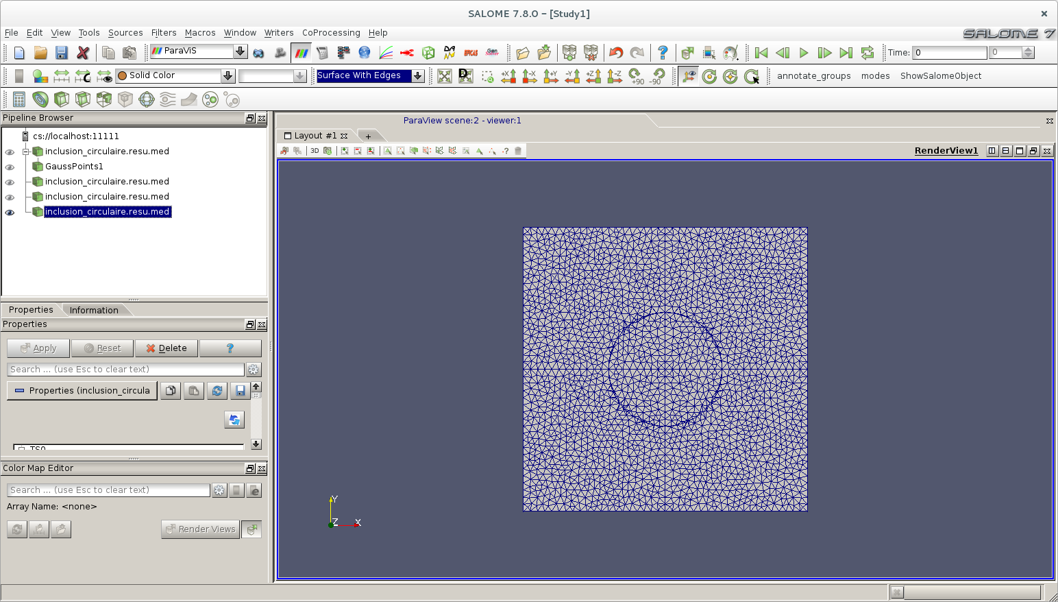
Figure 1.1: GUI of Salome Meca 7.8.0 displaying a 2D surface with mesh during postprocessing

1.5 ASTK

The provision of a multi-platform, multi-version IT tool that is used and co-developed by various teams has to be done through a Study and Developments Manager. This is ASTK’s aim: selecting the code version, defining the files comprised in a study, creating an overloaded version and accessing configuration management tools for developers. This interface uses network protocols for transferring files between clients and server, or for starting remote commands, including over the Internet. Users can easily distribute their data files and results to different machines as the interface ensures the transfer of files, including compressed ones, over the network.

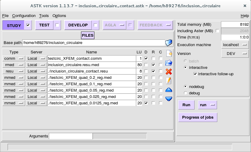
Figure 1.2: ASTK GUI letting the user select the mesh file and the output file along with the command file

2 Introduction to the Work

Due to a lot of attention focusing on the development of finite element methods for embedded interfaces, currently Nitsche’s method has been brought forward to enforce constraints, closed form analytical expressions for interfacial stabilization terms, and simple flux evaluation by the help of works done by Dolbow and others. By embedded, we refer to those methods in which the finite element mesh is not aligned with the interface geometry (for example X-FEM). Because the interfacial geometry can be arbitrary with respect to mesh, the robust enforcement of nonlinear constitutive laws(such as frictional contact) on embedded interfaces is a challenge that can be tackled with the help of Nitsche’s method.

Focusing on steady problems, but also presenting a case towards time dependent problems, the method has been implemented in the open source software Code-Aster. Two main cases of interface problems have been presented here. ’Jump’ problems, which deal with the interfacial problems concerning those in which the jump in the bulk primary (e.g. displacement, temperature) and/or secondary (e.g. traction, heat flux) field across the interface is known or given. The second class of problems are those in which primary field on the interface is given, referred to as ’Dirichlet’ problems.

The challenge with ’Jump’ type of problems, like a perfectly bonded material interface in composites, where both jump in displacement and traction across the interface vanish, the issue often amounts to the capturing the presence of slope discontinuities that arise due to the mismatch in material properties. With Nitsche’s method, more general case of non-zero jump can also be considered, which is more efficient than the enrichment with ’ridge’ function and simpler to implement than the blending of ramp function.

Gibbs-Thomson conditions arising in crystal growth and solidification problems, where the interfacial temperature is a function of the interfacial velocity and curvature, is an example of ’Dirichlet’ type of problems. The problems associated with such type of situations are usually due to unstable Lagrange multipliers even with the most convenient choice. Techniques such as penalty methods that may be adequate for enforcing constraints on stationary interfaces often prove to be lacking when it comes to yielding accurate, consistent flux quantities.

We also focus on developing the method taking into consideration some numerical issues like high sensitivity of normal flux, mild oscillations and non convergence issues. To balance this, we propose to calculate a modified numerical flux based on a weighted form. The advantages of this approach lies firstly in that it is a primal method that does not introduce additional degrees of freedom at the embedded interface. Secondly, we obtain stabilization parameters that are based on interfacial quantities of interest and not necessarily detrimental ’free’ parameter. Finally on extending the method to problems of contact, Nitsche’s method yields more accurate approximations of interfacial traction fields.

We implement Nitsche’s method focusing on discretization with a shifted basis enrichment. We also discuss the possibilities of implementing it in a non-linear Newton loop and obtain the basic matrix form to do so. We will look at an analytical solution and see how the method behaves in a simple problem. Finally, we will test the method in Code Aster on a circular inclusion problem and compare the results with those obtained by using Lagrange multipliers.

2.1 Nitsche’s Approach on General boundary condition

Consider the simple 2D Poisson problem: find $u$ such that

$$-\triangle u=f\,\,\,\,\mathrm{{in}}\,\Omega,$$ (2.1)

$$u=u_{0}\,\,\,\,\mathrm{on}\,\Gamma=\partial\Omega_{d},$$ (2.2)

$$\frac{\partial u}{\partial n}=g\,\,\,\,\mathrm{on}\,\Gamma=\partial\Omega_{n}.$$ (2.3)

where $\Omega$ is a bounded domain with polygonal boundary, $f\in L^{2}(\Omega)$, $u_{0}\in H^{1/2}(\Gamma)$, $g\in L^{2}(\Gamma)$ and $\epsilon\in\mathrm{R}$, $0\leq\epsilon\leq\infty$. If we consider the penalty method, by replacing the Dirichlet condition with:

$$\frac{\partial u}{\partial n} = \frac{1}{\epsilon}\left[(u_{0}-u)+\epsilon g\right]\,\,\,\,\mathrm{on}\,\Gamma,$$

$$= \frac{1}{\epsilon}\left[u_{0}-u\right]+g$$

where $\epsilon$ is a small parameter, which is problem dependent, and n is the outward normal. When $\epsilon\rightarrow 0$, the solution to the continuous problem converges to the solution of the Dirichlet problem (2.2) and $\epsilon\rightarrow\infty$ gives us the pure Neumann condition (2.3).

$$\epsilon\rightarrow 0 \Rightarrow u=u_{0}\,\,\,\,\mathrm{on}\,\Gamma$$

$$u-u_{0} = 0$$

$$\frac{\partial u}{\partial n} = 0$$

$$\epsilon\rightarrow\infty\Rightarrow\frac{\partial u}{\partial n}=g\,\,\,\,\mathrm{on}\,\Gamma$$

The drawbacks of this method are:

• nonconformity - the method requires coupling of the penalty parameter to the mesh size

• possible ill conditioning of the discrete system when $\epsilon$ is too small

Let us consider the variational form of the above simple problem. Multiply (2.1) with $v\in V_{h}$, integrating over the domain $\Omega$, and using Green’s formula, leads to

$$(\nabla u_{h},\nabla v)_{\Omega}-(\frac{\partial u_{h}}{\partial n},v)_{\Gamma}=(f,v)_{\Omega}$$ (2.5)

We now multiply the boundary condition (2.1) by $v$ and integrating over the domain which gives,

$$(\frac{\partial u_{h}}{\partial n},v)_{\Gamma}+\frac{1}{\epsilon}(u_{h},v)_{\Gamma}=\frac{1}{\epsilon}(u_{0},v)_{\Gamma}+(g,v)_{\Gamma}$$ (2.6)

Adding (2.5) and (2.6), the problem is equivalent to finding $u_{h}\in V_{h}$ such that

$$(\nabla u_{h},\nabla v)_{\Omega}\cancel{-(\frac{\partial u_{h}}{\partial n},v)_{\Gamma}}\cancel{+(\frac{\partial u_{h}}{\partial n},v)_{\Gamma}}+\frac{1}{\epsilon}(u_{h},v)_{\Gamma}=(f,v)_{\Omega}+\frac{1}{\epsilon}(u_{0},v)_{\Gamma}+(g,v)_{\Gamma}\,\,\,\,\forall v\in V_{h}$$ (2.7)

$$(\nabla u_{h},\nabla v)_{\Omega}+\frac{1}{\epsilon}(u_{h},v)_{\Gamma}=(f,v)_{\Omega}+\frac{1}{\epsilon}(u_{0},v)_{\Gamma}+(g,v)_{\Gamma}\,\,\,\,\forall v\in V_{h}$$ (2.8)

Following Juntenen and Stenberg formulations[1], consider, for simplicity, a regular shaped finite element partitioning ($\mathcal{T}_{h}$) of the domain ($\Omega\subset\text{R}^{N}$) into triangles or tetrahedra have been considered. The induced mesh is denoted by $\mathcal{G}_{h}$, on the boundary $\Gamma$. $K\in\mathcal{T}_{h}$ denotes the element of the mesh with diameter $h_{K}$ and $E\in\mathcal{G}_{h}$ denotes the edge or face with diameter $h_{E}$. Further definition consists of

$$h:=\text{max}\left\{h_{K}:K\in\mathcal{T}_{h}\right\}$$ (2.9)

and

$$V_{h}:=\left\{v\in H^{1}\left(\Omega\right):v_{|K}\in\mathcal{P}_{p}\left(K\right)\,\,\,\,\forall K\in\mathcal{T}_{h}\right\}$$ (2.10)

where $\mathcal{P}_{p}(K)$ is the space of polynomials of degree $p$. Integrating (2.6) over an element $E$ now gives us:

$$\epsilon(\frac{\partial u_{h}}{\partial n},v)_{E}+(u_{h},v)_{E}=(u_{0},v)_{E}+\epsilon(g,v)_{E}$$ (2.11)

We can write now (2.11) as

$$\sum_{E\in\mathcal{G}_{h}}\frac{1}{\epsilon+\gamma h_{E}}\left\{\epsilon(\frac{\partial u_{h}}{\partial n},v)_{E}+(u_{h},v)_{E}\right\}=\sum_{E\in\mathcal{G}_{h}}\frac{1}{\epsilon+\gamma h_{E}}\left\{(u_{0},v)_{E}+\epsilon(g,v)_{E}\right\}$$ (2.12)

where $\gamma$ is a positive parameter, known as the stability parameter.

Also from (2.6), we can write, by multiplying the condition with $\frac{\partial v}{\partial n}$:

$$\epsilon(\frac{\partial u_{h}}{\partial n},\frac{\partial v}{\partial n})_{E}+(u_{h},\frac{\partial v}{\partial n})_{E}=(u_{0},\frac{\partial v}{\partial n})_{E}+\epsilon(g,\frac{\partial v}{\partial n})_{E}$$ (2.13)

Similarly like (2.12), we can write:

$$\sum_{E\in\mathcal{G}_{h}}-\frac{\gamma h_{E}}{\epsilon+\gamma h_{E}}\left\{\epsilon(\frac{\partial u_{h}}{\partial n},\frac{\partial v}{\partial n})_{E}+(u_{h},\frac{\partial v}{\partial n})_{E}\right\}=\sum_{E\in\mathcal{G}_{h}}-\frac{\gamma h_{E}}{\epsilon+\gamma h_{E}}\left\{(u_{0},\frac{\partial v}{\partial n})_{E}+\epsilon(g,\frac{\partial v}{\partial n})_{E}\right\}$$ (2.14)

Adding (2.5), (2.12) and (2.14), we get:

$$(\nabla u_{h},\nabla v)_{\Omega}-(\frac{\partial u_{h}}{\partial n},v)_{\Gamma} + \sum_{E\in\mathcal{G}_{h}}\frac{1}{\epsilon+\gamma h_{E}}\left\{\epsilon(\frac{\partial u_{h}}{\partial n},v)_{E}+(u_{h},v)_{E}\right\}$$

$$+\sum_{E\in\mathcal{G}_{h}}-\frac{\gamma h_{E}}{\epsilon+\gamma h_{E}}\left\{\epsilon(\frac{\partial u_{h}}{\partial n},\frac{\partial v}{\partial n})_{E}+(u_{h},\frac{\partial v}{\partial n})_{E}\right\}$$

$$=(f,v)_{\Omega}+\sum_{E\in\mathcal{G}_{h}}\frac{1}{\epsilon+\gamma h_{E}}\left\{(u_{0},v)_{E}+\epsilon(g,v)_{E}\right\}+\sum_{E\in\mathcal{G}_{h}}-\frac{\gamma h_{E}}{\epsilon+\gamma h_{E}}\left\{(u_{0},\frac{\partial v}{\partial n})_{E}+\epsilon(g,\frac{\partial v}{\partial n})_{E}\right\}$$ (2.15)

Finally, we find $u_{h}\in V_{h}$ such that:

$$\mathcal{B}_{h}(u_{h},v)=\mathcal{F}_{h}(v)\,\,\,\,\forall v\in V_{h}$$ (2.16)

with:

$$\mathcal{B}_{h}(u,v) = (\nabla u,\nabla v)_{\Omega}$$

$$+\sum_{E\in\mathcal{G}_{h}}\left\{-\frac{\gamma h_{E}}{\epsilon+\gamma h_{E}}\left[\left\langle\frac{\partial u}{\partial n},v\right\rangle_{E}+\left\langle u,\frac{\partial v}{\partial n}\right\rangle_{E}\right]+\frac{1}{\epsilon+\gamma h_{E}}\left\langle u,v\right\rangle_{E}-\frac{\epsilon\gamma h_{E}}{\epsilon+\gamma h_{E}}\left\langle\frac{\partial u}{\partial n},\frac{\partial v}{\partial n}\right\rangle_{E}\right\}$$

and:

$$\mathcal{F}_{h}(v) = (f,v)_{\Omega}$$

$$+\sum_{E\in\mathcal{G}_{h}}\left\{\frac{1}{\epsilon+\gamma h_{E}}\left\langle u_{0},v\right\rangle_{E}-\frac{\gamma h_{E}}{\epsilon+\gamma h_{E}}\left\langle u_{0},\frac{\partial v}{\partial n}\right\rangle_{E}+\frac{\epsilon}{\epsilon+\gamma h_{E}}\left\langle g,v\right\rangle_{E}-\frac{\epsilon\gamma h_{E}}{\epsilon+\gamma h_{E}}\left\langle g,\frac{\partial v}{\partial n}\right\rangle_{E}\right\}$$

We can use Nitsche’s technique at the limiting condition $\epsilon=0$. This method can also be extended to the whole range of boundary conditions, with $\epsilon\geq 0$.

If we put $\gamma=0$ in (2.1), we can see that

$$(\nabla u_{h},\nabla v)_{\Omega}-(\frac{\partial u_{h}}{\partial n},v)_{\Gamma} + \sum_{E\in\mathcal{G}_{h}}\frac{1}{\epsilon+\cancel{\gamma h_{E}}}\left\{\epsilon(\frac{\partial u_{h}}{\partial n},v)_{E}+(u_{h},v)_{E}\right\}$$

$$\cancel{+\sum_{E\in\mathcal{G}_{h}}-\frac{\gamma h_{E}}{\epsilon+\gamma h_{E}}\left\{\epsilon(\frac{\partial u_{h}}{\partial n},\frac{\partial v}{\partial n})_{E}+(u_{h},\frac{\partial v}{\partial n})_{E}\right\}}$$

$$=(f,v)_{\Omega}+\sum_{E\in\mathcal{G}_{h}}\frac{1}{\epsilon+\cancel{\gamma h_{E}}}\left\{(u_{0},v)_{E}+\epsilon(g,v)_{E}\right\}+\cancel{\sum_{E\in\mathcal{G}_{h}}-\frac{\gamma h_{E}}{\epsilon+\gamma h_{E}}\left\{(u_{0},\frac{\partial v}{\partial n})_{E}+\epsilon(g,\frac{\partial v}{\partial n})_{E}\right\}}$$ (2.19)

$$(\nabla u_{h},\nabla v)_{\Omega}\cancel{-(\frac{\partial u_{h}}{\partial n},v)_{\Gamma}}\cancel{+\sum_{E\in\mathcal{G}_{h}}(\frac{\partial u_{h}}{\partial n},v)_{E}}+\sum_{E\in\mathcal{G}_{h}}\frac{1}{\epsilon}(u_{h},v)_{E}=(f,v)_{\Omega}+\sum_{E\in\mathcal{G}_{h}}\frac{1}{\epsilon}(u_{0},v)_{E}+\sum_{E\in\mathcal{G}_{h}}(g,v)_{E}$$ (2.20)

$$(\nabla u_{h},\nabla v)_{\Omega}+\sum_{E\in\mathcal{G}_{h}}\frac{1}{\epsilon}(u_{h},v)_{E}=(f,v)_{\Omega}+\sum_{E\in\mathcal{G}_{h}}\frac{1}{\epsilon}(u_{0},v)_{E}+\sum_{E\in\mathcal{G}_{h}}(g,v)_{E}$$ (2.21)

which is the same as the traditional form obtained in (2.8) with . With $\gamma=0,$ the system may become ill-conditioned at small $\epsilon>0$ values.

For a stabilized method with $\gamma>0,$ at the limit $\epsilon=0,$ we get the Dirichlet problem with Nitsche’s application: find $u_{h}\in V_{h}$ such that

$$(\nabla u,\nabla v)_{\Omega}-\left\langle\frac{\partial u_{h}}{\partial n},v\right\rangle_{\Gamma}-\left\langle u_{h},\frac{\partial v}{\partial n}\right\rangle_{\Gamma} +\sum_{E\in\mathcal{G}_{h}}\frac{1}{\gamma h_{E}}\left\langle u_{h},v\right\rangle_{E}$$

$$=(f,v)_{\Omega}-\left\langle u_{0},\frac{\partial v}{\partial n}\right\rangle_{\Gamma} +\sum_{E\in\mathcal{G}_{h}}\frac{1}{\gamma h_{E}}\left\langle u_{0},v\right\rangle_{E} \forall v\in V_{h}$$ (2.22)

and at $\epsilon\rightarrow\infty,$ it is a pure Neumann problem that needs to be solved: find $u_{h}\in V_{h}$ such that

$$(\nabla u,\nabla v)_{\Omega}+\sum_{E\in\mathcal{G}_{h}}\gamma h_{E}\left\langle\frac{\partial u_{h}}{\partial n},\frac{\partial v}{\partial n}\right\rangle_{E}=(f,v)_{\Omega}+(g,v)_{\Gamma}-\sum_{E\in\mathcal{G}_{h}}\gamma h_{E}\left\langle g,\frac{\partial v}{\partial n}\right\rangle_{E}$$ (2.23)

This requires that the data satisfy

$$\left(f,1\right)_{\Omega}+\left\langle g,1\right\rangle_{\Gamma}=0$$ (2.24)

and this condition is not violated in the above formulations.

2.2 Comparison with other approaches

Consider the governing equation

$$-\nabla\centerdot(\kappa\nabla u)=f\,\,\,\,\mathrm{{in}}\,\Omega,$$ (2.25)

$$u=u_{0}\,\,\,\,\mathrm{on}\,\Gamma=\partial\Omega$$ (2.26)

We will now discuss some techniques to weakly impose Dirichlet constraints on embedded surfaces and try to develop one method from another while briefly discussing the merits of one over the other. This part is based on the work done by Sanders, Dolbow and Laursen.[2]

We consider $\mathbf{n}$ the unit normal to $\Gamma$ which points out of $\Omega$. The primal variable of $u$ is defined in $\mathbb{U},$ and its variation $\delta u$ is an element of $\mathbb{U}_{0}$:

$$\mathbb{U}=\left\{u\in H^{1}(\Omega),u=u_{0}\,\mathrm{on}\,\Gamma\right\},$$

$$\mathbb{U}_{0}=\left\{u\in H^{1}(\Omega),u=0\,\mathrm{on}\,\Gamma\right\}.$$

The potential energy of such a system can be given by

$$\Pi(u)=\frac{1}{2}\int_{\Omega}\nabla u\centerdot\kappa\nabla u\mathrm{d\Omega}-\int_{\Omega}fu\mathrm{d}\Omega$$ (2.27)

The solution $u$ minimizes this potential energy under Dirichlet constraints. We can transform this constrained problem into an unconstrained one by using Lagrange multipliers. For the constraint to be enforced, let’s build the Lagrangian of the system, $\mathcal{L}$, by adding the work of the Lagrange multipliers, $\lambda$ in $\mathbb{L}=H^{-1/2}(\Gamma^{*})$:

$$\mathcal{L}(u,\lambda) = \Pi(u)+\int_{\Gamma}\lambda(u-u_{0})\mathrm{d}\mathrm{\Gamma}$$ (2.28)

$$= \frac{1}{2}\int_{\Omega}\nabla u\centerdot\kappa\nabla u\mathrm{d\Omega}-\int_{\Omega}fu\mathrm{d}\Omega+\int_{\Gamma}\lambda(u-u_{0})\mathrm{d}\mathrm{\Gamma}$$

We get a dual variational formulation due to the stationarity of $\mathcal{L}$: for all $(\delta u,\delta\lambda)\in\mathbb{U}_{0}\times\mathbb{L}$ find $(u,\lambda)\in\mathbb{U\times L}$, such that:

$$\delta\mathcal{L}=\int_{\Omega}\nabla\delta u\centerdot\kappa\nabla u\mathrm{d\Omega}-\int_{\Omega}\delta uf\mathrm{d\Omega}+\int_{\Gamma}\lambda\delta u\mathrm{d}\mathrm{\Gamma}+\int_{\Gamma}\delta\lambda(u-u_{0})\mathrm{d}\mathrm{\Gamma}=0$$ (2.29)

(Lagrangian method)

Here $\lambda$ and $u$ cannot be independently determined. And this brings about a lot of stability issues. We can solve this by the use of penalty methods. We can interpret Lagrange multipliers as flux imposed on the boundary condition. This leads us to establish $\lambda=-\kappa\nabla u\centerdot\mathrm{\mathbf{n}}$, the flux. Now we assume that the flux can be approximated in a spring like form $\kappa\nabla u\centerdot\mathrm{\mathbf{n}}\approx-\epsilon(u-u_{0}).$ The penalty potential is now,

$$\Pi^{\mathrm{pen}}(u) = \Pi(u)+\int_{\Gamma}\frac{\epsilon}{2}(u-u_{0})(u-u_{0})\mathrm{d}\mathrm{\Gamma}$$ (2.30)

$$= \Pi(u)+\int_{\Gamma}\frac{\epsilon}{2}(u-u_{0})^{2}\mathrm{d}\mathrm{\Gamma}$$

$$= \frac{1}{2}\int_{\Omega}\nabla u\centerdot\kappa\nabla u\mathrm{d\Omega}-\int_{\Omega}fu\mathrm{d}\Omega+\int_{\Gamma}\frac{\epsilon}{2}(u-u_{0})^{2}\mathrm{d}\mathrm{\Gamma}$$

The primal penalty variational form is given by: for all $\delta u\in\mathbb{U}_{0}$ find $u\in\mathbb{U}$, such that

$$\delta\Pi^{\mathrm{pen}}=\int_{\Omega}\nabla\delta u\centerdot\kappa\nabla u\mathrm{d\Omega}-\int_{\Omega}\delta uf\mathrm{d\Omega}+\int_{\Gamma}\delta u\epsilon(u-u_{0})\mathrm{d}\mathrm{\Gamma}=0$$ (2.31)

(Penalty method)

This is not variationally consistent, as the desired problem is solved only in the limiting case when $\epsilon\rightarrow\infty$.

Another standard way to improve the behavior of a Lagrangian method is to stabilize it with a penalty term. This gives the augmented Lagrangian approach.

$$\mathcal{L}^{\mathrm{aug}}(u,\lambda) = \Pi(u)+\int_{\Gamma}\lambda(u-u_{0})\mathrm{d}\mathrm{\Gamma}+\int_{\Gamma}\frac{\epsilon}{2}(u-u_{0})^{2}\mathrm{d}\mathrm{\Gamma}$$ (2.32)

$$= \frac{1}{2}\int_{\Omega}\nabla u\centerdot\kappa\nabla u\mathrm{d\Omega}-\int_{\Omega}fu\mathrm{d}\Omega+\int_{\Gamma}\lambda(u-u_{0})\mathrm{d}\mathrm{\Gamma}+\int_{\Gamma}\frac{\epsilon}{2}(u-u_{0})^{2}\mathrm{d}\mathrm{\Gamma}$$

Here the penalty stiffness can be seen as the stabilization parameter, which does not need large values of it. The dual variational form: for all $(\delta u,\delta\lambda)\in\mathbb{U}_{0}\times\mathbb{L}$ find $(u,\lambda)\in\mathbb{U\times L}$, such that:

$$\delta\mathcal{L}^{\mathrm{aug}} = \int_{\Omega}\nabla\delta u\centerdot\kappa\nabla u\mathrm{d\Omega}-\int_{\Omega}\delta uf\mathrm{d\Omega}+\int_{\Gamma}\delta u\lambda\mathrm{d}\mathrm{\Gamma}+\int_{\Gamma}\delta\lambda(u-u_{0})\mathrm{d}\mathrm{\Gamma}+\int_{\Gamma}\delta u\epsilon(u-u_{0})\mathrm{d}\mathrm{\Gamma}$$ (2.33)

$$= \int_{\Omega}\nabla\delta u\centerdot\kappa\nabla u\mathrm{d\Omega}-\int_{\Omega}\delta uf\mathrm{d\Omega}+\int_{\Gamma}\delta u(\lambda+\epsilon(u-u_{0}))\mathrm{d}\mathrm{\Gamma}+\int_{\Gamma}\delta\lambda(u-u_{0})\mathrm{d}\mathrm{\Gamma}=0$$

(Augmented Lagrangian method)

In the same manner to obtain a penalty variational form from a Lagrangian one, we can utilize the flux relation $\lambda=-\kappa\nabla u\centerdot\mathrm{\mathbf{n}}$ to obtain the potential function that forms the basis of Nitsche’s method.

$$\Pi^{\mathrm{Nit}}(u) = \Pi(u)-\int_{\Gamma}(u-u_{0})\kappa\nabla u\centerdot\mathrm{\mathbf{n}}\mathrm{d}\mathrm{\Gamma}+\int_{\Gamma}\frac{\epsilon}{2}(u-u_{0})^{2}\mathrm{d}\mathrm{\Gamma}$$ (2.34)

$$= \frac{1}{2}\int_{\Omega}\nabla u\centerdot\kappa\nabla u\mathrm{d\Omega}-\int_{\Omega}fu\mathrm{d}\Omega-\int_{\Gamma}(u-u_{0})\kappa\nabla u\centerdot\mathrm{\mathbf{n}}\mathrm{d}\mathrm{\Gamma}+\int_{\Gamma}\frac{\epsilon}{2}(u-u_{0})^{2}\mathrm{d}\mathrm{\Gamma}$$

We get one-field symmetric variational formulation: for all $\delta u\in\mathbb{U}_{0}$ find $u\in\mathbb{U}$, such that :

$$\delta\Pi^{\mathrm{Nit}}(u) = \int_{\Omega}\nabla\delta u\centerdot\kappa\nabla u\mathrm{d\Omega}-\int_{\Omega}\delta uf\mathrm{d\Omega}-\int_{\Gamma}\delta u\kappa\nabla u\centerdot\mathrm{\mathbf{n}}\mathrm{d}\mathrm{\Gamma}$$ (2.35)

$$-\int_{\Gamma}(u-u_{0})\kappa\nabla\delta u\centerdot\mathrm{\mathbf{n}}\mathrm{d}\mathrm{\Gamma}+\int_{\Gamma}\delta u\epsilon(u-u_{0})\mathrm{d}\mathrm{\Gamma}=0$$

(Nitsche’s method)

Rearranging, we can write:

$$\int_{\Omega}\nabla\delta u\centerdot\kappa\nabla u\mathrm{d\Omega}-\int_{\Gamma}\delta u\kappa\nabla u\centerdot\mathrm{\mathbf{n}}\mathrm{d}\mathrm{\Gamma}-\int_{\Gamma}(u-u_{0})\kappa\nabla\delta u\centerdot\mathrm{\mathbf{n}}\mathrm{d}\mathrm{\Gamma}+\int_{\Gamma}\delta u\epsilon(u-u_{0})\mathrm{d}\mathrm{\Gamma}=\int_{\Omega}\delta uf\mathrm{d\Omega}$$

or:

$$\int_{\Omega}\nabla\delta u\centerdot\kappa\nabla u\mathrm{d\Omega}-\int_{\Gamma}\delta u\kappa\nabla u\centerdot\mathrm{\mathbf{n}}\mathrm{d}\mathrm{\Gamma}-\int_{\Gamma}u\kappa\nabla\delta u\centerdot\mathrm{\mathbf{n}}\mathrm{d}\mathrm{\Gamma}+\int_{\Gamma}\delta u\epsilon u\mathrm{d}\mathrm{\Gamma}$$

$$= \int_{\Omega}\delta uf\mathrm{d\Omega}- \int_{\Gamma}u_{0}\kappa\nabla\delta u\centerdot\mathrm{\mathbf{n}}\mathrm{d}\mathrm{\Gamma}+\int_{\Gamma}\delta u\epsilon u_{0}\mathrm{d}\mathrm{\Gamma}$$ (2.36)

If we compare this with (2.22), we can see that $\epsilon$ is similar to the term $\sum_{E\in\mathcal{G}_{h}}\frac{1}{\gamma h_{E}}$.

2.3 Application to Interfaces

We can now extend Nitsche’s method to an interface made of two materials or even to a crack that divides the surface. We develop this based on the works of Dolbow and Harari.[3]

Find $u\in\mathbb{U}$, such that:

$$a_{b}(v,u)+a_{i}(v,u)=l_{b}(v)+l_{i}(v)\,\,\,\,\forall v\in\mathbb{U}_{0}$$ (2.37)

where now:

$$a_{b}(v,u)=\int_{\Omega}\nabla v\centerdot\kappa\nabla u\mathrm{d\Omega}$$

and:

$$l_{b}(v)=\int_{\Omega}vf\mathrm{d\Omega}$$

are the standard bulk contributions from (2.36), with:

$$\mathbb{U}_{\,\,} = \left\{u\in H^{1}(\Omega^{-}\cup\Omega^{+}),u=u_{0}\,\mathrm{on}\,\Gamma,\mbox{ may be discontinuous on }\mathcal{S}\right\}\mbox{ and}$$

$$\mathbb{U}_{0} = \left\{v\in H^{1}(\Omega^{-}\cup\Omega^{+}),v=0\,\mathrm{on}\,\Gamma,\mbox{ may be discontinuous on }\mathcal{S}\right\}.$$

$a_{i}(v,u)$ and $l_{i}(v)$ are the interfacial contributions which depend on the case being considered. These terms are obtained by utilizing the boundary conditions in a similar manner to that in (2.36), but on the interface, if we can consider the domain $\Omega$ to be divided by an interface $\mathcal{S}$.

Dirichlet condition (ex. crack surface)

Consider the boundary conditions:

$$u^{+}=g^{+},\,\,\,\,u^{-}=g^{-}\mbox{\,\,\,\,\ on }\mathcal{\mathcal{S}}$$

where $g^{+}$ and $g^{-}$ are assumed to be sufficiently smooth functions of the position on the interface. $u^{+}$ and $u^{-}$ are limiting values of the field $u$ as the interface is approached from either $\Omega^{+}$ or $\Omega^{-}$, respectively. Approaching this problem as two one-sided problems, we can write

$$a_{i}(v,u) = a_{i}(v,u)^{+}+a_{i}(v,u)^{-}$$ (2.38)

$$l_{i}(v) = l_{i}(v)^{+}+l_{i}(v)^{-}$$ (2.39)

We choose the interfacial normal $\mathrm{\mathbf{n}}$ as pointing outwardly from $\Omega^{+}$. This gives us, from (2.36),

$$a_{i}(v,u)^{+} = -\int_{\mathcal{S}}v^{+}(\kappa^{+}\nabla u^{+}\centerdot\mathrm{\mathbf{n}})\mathrm{d}\mathrm{\Gamma}-\int_{\mathcal{S}}u^{+}(\kappa^{+}\nabla v^{+}\centerdot\mathrm{\mathbf{n}})\mathrm{d}\mathrm{\Gamma}+\int_{\mathcal{S}}v^{+}\alpha^{+}u^{+}\mathrm{d}\mathrm{\Gamma}$$ (2.40)

$$a_{i}(v,u)^{-} = -\int_{\mathcal{S}}v^{-}(\kappa^{-}\nabla u^{-}\centerdot\left(-\mathrm{\mathbf{n}}\right))\mathrm{d}\mathrm{\Gamma}-\int_{\mathcal{S}}u^{-}(\kappa^{-}\nabla v^{-}\centerdot\left(-\mathrm{\mathbf{n}}\right))\mathrm{d}\mathrm{\Gamma}+\int_{\mathcal{S}}v^{-}\alpha^{-}u^{-}\mathrm{d}\mathrm{\Gamma}$$ (2.41)

$$= \int_{\mathcal{S}}v^{-}(\kappa^{-}\nabla u^{-}\centerdot\mathrm{\mathbf{n}})\mathrm{d}\mathrm{\Gamma}+\int_{\mathcal{S}}u^{-}(\kappa^{-}\nabla v^{-}\centerdot\mathrm{\mathbf{n}})\mathrm{d}\mathrm{\Gamma}+\int_{\mathcal{S}}v^{-}\alpha^{-}u^{-}\mathrm{d}\mathrm{\Gamma}$$

$$l_{i}(v)^{+} = -\int_{\mathcal{S}}g^{+}(\kappa^{+}\nabla v^{+}\centerdot\mathrm{\mathbf{n}})\mathrm{d}\mathrm{\Gamma}+\int_{\mathcal{S}}v^{+}\alpha^{+}g^{+}\mathrm{d}\mathrm{\Gamma}$$ (2.42)

$$l_{i}(v)^{-} = -\int_{\mathcal{S}}g^{-}(\kappa^{-}\nabla v^{-}\centerdot\left(-\mathrm{\mathbf{n}}\right))\mathrm{d}\mathrm{\Gamma}+\int_{\mathcal{S}}v^{-}\alpha^{-}g^{-}\mathrm{d}\mathrm{\Gamma}$$ (2.43)

$$= \int_{\mathcal{S}}g^{-}(\kappa^{-}\nabla v^{-}\centerdot\mathrm{\mathbf{n}})\mathrm{d}\mathrm{\Gamma}+\int_{\mathcal{S}}v^{-}\alpha^{-}g^{-}\mathrm{d}\mathrm{\Gamma}$$

where we have chosen $\alpha^{+}$ and $\alpha^{-}$ as the stabilization parameters for the $\Omega^{+}$ and $\Omega^{-}$ domains respectively (Figure 2.1).

Figure 2.1: Notation for two-sided problem

With a Dirichlet condition of this type, a jump $\bar{\mathrm{j}}$ in the flux, if it exists, is unknown and represents a quantity of interest. This is because we have assumed here that the two domains are completely different problems. If we consider $\mathcal{L}$ as a portion of the interface, with $\mathcal{B}=\mathcal{B}^{+}\cup\mathcal{B}^{-}$ being the supports of the weight function $v_{d}$ that covers smoothly, a point $\mathbf{x}_{\mbox{d}}$ on the interface, and $\mathcal{L}=\mathcal{B}\cap\mathcal{S}$, we obtain:

$$\int_{\mathcal{L}}v_{d}\bar{\mathrm{j}}\mbox{d}\Gamma = \int_{\mathcal{B}}v_{d}f\,\mbox{d}\Omega-\int_{\mathcal{B}}\nabla v_{d}\kappa\nabla u\,\mbox{d}\Omega$$ (2.44)

$$= \int_{\mathcal{B}}v_{d}^{+}f\,\mbox{d}\Omega-\int_{\mathcal{B}}\nabla v_{d}^{+}\kappa^{+}\nabla u^{+}\,\mbox{d}\Omega+\int_{\mathcal{B}}v_{d}^{-}f\,\mbox{d}\Omega-\int_{\mathcal{B}}\nabla v_{d}^{-}\kappa^{-}\nabla u^{-}\,\mbox{d}\Omega$$ (2.45)

with $\left[\left[\kappa\nabla u\right]\right]\centerdot\mathbf{n}=\left(\kappa\nabla u^{+}-\kappa\nabla u^{-}\right)\centerdot\mathbf{n}=\bar{\mathrm{j}}$ which can be used to approximate the jump in flux across the portion of interface considered.

Jump Condition (ex. a bimaterial interface)

Consider the given problem

$$-\nabla\centerdot(\kappa^{+}\nabla u)=f\mbox{ in }\Omega^{+}$$

$$-\nabla\centerdot(\kappa^{-}\nabla u)=f\mbox{ in }\Omega^{-}$$

with

$$u=u_{0}\,\,\,\,\mathrm{on}\,\Gamma=\partial\Omega$$

$$\left[\left[u\right]\right] = \bar{\mathrm{i}}\,\,\,\,\mathrm{on}\,\mathcal{S}$$

$$u^{+}-u^{-} = \bar{\mathrm{i}}$$

$$\left[\left[\kappa\nabla u\right]\right]\centerdot\mathbf{n} = \bar{\mathrm{j}}\,\,\,\,\mathrm{on}\,\mathcal{S}$$

$$\left(\kappa^{+}\nabla u^{+}-\kappa^{-}\nabla u^{-}\right).\mathbf{n} = \bar{\mathrm{j}}$$

where $\mathbf{n}$ is considered to point outwards from $\Omega^{+}$.

$$\left(\kappa\nabla u\right).\mathbf{n}_{\text{0}}=0\mbox{ on }\Gamma=\partial\Omega_{n}$$

Consider the domain $\Omega^{+}$. We can try to obtain the weak Galerkin formulation.

$$-\int_{\Omega^{+}}v^{+}\nabla\centerdot\left(\kappa^{+}\nabla u^{+}\right)=\int_{\Omega^{+}}v^{+}f\,\mbox{d}\Omega$$ (2.46)

We can write:

$$\int_{\Omega^{+}}\nabla v^{+}.\left(\kappa^{+}\nabla u^{+}\right)-\int_{\Omega^{+}}\nabla.\left(v^{+}\kappa^{+}\nabla u^{+}\right)=\int_{\Omega^{+}}v^{+}f\,\mbox{d}\Omega$$

from divergence theorem. And also:

$$\int_{\Omega^{+}}\nabla.\left(v^{+}\kappa^{+}\nabla u^{+}\right)=\int_{S}v^{+}\left(\kappa^{+}\nabla u^{+}.\mathbf{n}\right)+\cancel{\int_{\partial\Omega_{n}}v^{+}\left(\kappa^{+}\nabla u^{+}.\mathbf{n}_{0}\right)}$$

Thus weak Galerkin formulation of the above problem gives us: find $u\in\mathbb{U}$ such that

$$\int_{\Omega^{+}}\nabla v^{+}.\kappa^{+}\nabla u^{+}\mbox{d}\Omega-\int_{\mathcal{S}}v^{+}(\kappa^{+}\nabla u^{+}.\mathbf{n})\mbox{d}\Gamma=\int_{\Omega^{+}}v^{+}f\,\mbox{d}\Omega\mbox{ }\forall v\in\mathbb{U}_{0}$$ (2.47)

and similarly on domain $\Omega^{-}$,

$$\int_{\Omega^{-}}\nabla v^{-}.\kappa^{-}\nabla u^{-}\mbox{d}\Omega+\int_{\mathcal{S}}v^{-}(\kappa^{-}\nabla u^{-}.\mathbf{n})\mbox{d}\Gamma=\int_{\Omega^{-}}v^{-}f\,\mbox{d}\Omega\mbox{ }\forall v\in\mathbb{U}_{0}$$ (2.48)

We have considered the problem separately in the two domains which has resulted in the separation of the jump in flux. Adding the two equations gives:

$$\int_{\Omega}\nabla v.\kappa\nabla u\mbox{d}\Omega-\int_{\mathcal{S}}\left[v^{+}(\kappa^{+}\nabla u^{+}.\mathbf{n})-v^{-}(\kappa^{-}\nabla u^{-}.\mathbf{n})\right]\mbox{d}\Gamma=\int_{\Omega}vf\mbox{d}\Omega$$ (2.49)

Also

$$\kappa^{+}\nabla u^{+}=<\kappa\nabla u>+\frac{1}{2}[[\kappa\nabla u]]$$ (2.50)

and

$$\kappa^{-}\nabla u^{-}=<\kappa\nabla u>-\frac{1}{2}[[\kappa\nabla u]]$$ (2.51)

Substituting these in the weak formulation gives:

$$\int_{\Omega}\nabla v.\kappa\nabla u\mbox{d}\Omega-\int_{\mathcal{S}}\left[v^{+}\left(\left(<\kappa\nabla u>+\frac{1}{2}[[\kappa\nabla u]]\right).\mathbf{n}\right)-v^{-}\left(\left(<\kappa\nabla u>-\frac{1}{2}[[\kappa\nabla u]]\right).\mathbf{n}\right)\right]\mbox{d}\Gamma=\int_{\Omega}vf\,\mbox{d}\Omega$$

$$\int_{\Omega}\nabla v.\kappa\nabla u\mbox{d}\Omega-\int_{\mathcal{S}}\left[\frac{1}{2}v^{+}[[\kappa\nabla u]].\mathbf{n}+v^{+}<\kappa\nabla u>.\mathbf{n}+\frac{1}{2}v^{-}[[\kappa\nabla u]].\mathbf{n}-v^{-}<\kappa\nabla u>.\mathbf{n}\right]\mbox{d}\Gamma=\int_{\Omega}vf\,\mbox{d}\Omega$$

$$\int_{\Omega}\nabla v.\kappa\nabla u\mbox{d}\Omega-\int_{\mathcal{S}}\left[\frac{1}{2}(v^{+}+v^{-})[[\kappa\nabla u]].\mathbf{n}+(v^{+}-v^{-})<\kappa\nabla u>.\mathbf{n}\right]\mbox{d}\Gamma=\int_{\Omega}vf\,\mbox{d}\Omega$$

$$\int_{\Omega}\nabla v.\kappa\nabla u\mbox{d}\Omega-\int_{\mathcal{S}}\left[\left\langle v\right\rangle\bar{\mathrm{j}}+\left[\left[v\right]\right]<\kappa\nabla u>.\mathbf{n}\right]\mbox{d}\Gamma=\int_{\Omega}vf\,\mbox{d}\Omega$$

$$\int_{\Omega}\nabla v.\kappa\nabla u\mbox{d}\Omega-\int_{\mathcal{S}}\left[\left[v\right]\right]<\kappa\nabla u>.\mathbf{n}+\int_{\mathcal{S}}\frac{v^{-}}{2}\left(\kappa^{-}\nabla u^{-}\centerdot\mathrm{\mathbf{n}}\right)\mathrm{d}\mathrm{\Gamma}\mbox{d}\Gamma=\int_{\Omega}f\,\mbox{d}\Omega+\int_{\mathcal{S}}\left\langle v\right\rangle\bar{\mathrm{j}}\mbox{d}\Gamma$$ (2.52)

Now we can introduce Nitsche’s terms and the corresponding stabilization terms in this equation to get the variational form and maintain the symmetric nature of the system with Nitsche’s approach:

$$\int_{\Omega}\nabla v.\kappa\nabla u\mbox{d}\Omega-\int_{\mathcal{S}}\left[\left[v\right]\right]<\kappa\nabla u>.\mathbf{n}\mbox{d}\Gamma-\int_{\mathcal{S}}[[u]]<\kappa\nabla v>\centerdot\mathrm{\mathbf{n}}\mathrm{d}\mathrm{\Gamma}+\int_{\mathcal{S}}[[v]]\alpha[[u]]\mathrm{d}\mathrm{\Gamma}$$

$$=\int_{\Omega}vf\,\mbox{d}\Omega+\int_{\mathcal{S}}\left\langle v\right\rangle\bar{\mathrm{j}}\mbox{d}\Gamma-\int_{\mathcal{S}}\bar{\mbox{i}}<\kappa\nabla v>\centerdot\mathrm{\mathbf{n}}\mathrm{d}\mathrm{\Gamma}+\int_{\mathcal{S}}[[v]]\alpha\,\bar{\mbox{i}}\,\mathrm{d}\mathrm{\Gamma}$$ (2.53)

This form is both variationally consistent as well as symmetric. Thus, we can write

$$a_{i}(v,u) = -\int_{\mathcal{S}}[[v]]<\kappa\nabla u>\centerdot\mathrm{\mathbf{n}}\mathrm{d}\mathrm{\Gamma}-\int_{\mathcal{S}}[[u]]<\kappa\nabla v>\centerdot\mathrm{\mathbf{n}}\mathrm{d}\mathrm{\Gamma}+\int_{\mathcal{S}}[[v]]\alpha[[u]]\mathrm{d}\mathrm{\Gamma}$$ (2.54)

$$l_{i}(v) = -\int_{\mathcal{S}}\bar{\mbox{i}}<\kappa\nabla v>\centerdot\mathrm{\mathbf{n}}\mathrm{d}\mathrm{\Gamma}+\int_{\mathcal{S}}[[v]]\alpha\,\bar{\mbox{i}}\,\mathrm{d}\mathrm{\Gamma}+\int_{\mathcal{S}}<v>\bar{\mbox{j}}\mathrm{d}\mathrm{\Gamma}$$ (2.55)

$\alpha$ is the integrated stabilizing term for this form here.

Comparison

If we expand the jump condition relations, we have, from (2.54) and (2.55),

$$a_{i}(v,u) = -\int_{\mathcal{S}}\frac{\left(v^{+}-v^{-}\right)}{2}\left(\kappa^{+}\nabla u^{+}\centerdot\mathrm{\mathbf{n}}+\kappa^{-}\nabla u^{-}\centerdot\mathrm{\mathbf{n}}\right)\mathrm{d}\mathrm{\Gamma}$$

$$-\int_{\mathcal{S}}\frac{\left(u^{+}-u^{-}\right)}{2}\left(\kappa^{+}\nabla v^{+}\centerdot\mathrm{\mathbf{n}}+\kappa^{-}\nabla v^{-}\centerdot\mathrm{\mathbf{n}}\right)\mathrm{d}\mathrm{\Gamma}+\int_{\mathcal{S}}\left(v^{+}-v^{-}\right)\alpha(u^{+}-u^{-})\mathrm{d}\mathrm{\Gamma}$$

$$= -\int_{\mathcal{S}}\frac{v^{+}}{2}\left(\kappa^{+}\nabla u^{+}\centerdot\mathrm{\mathbf{n}}\right)\mathrm{d}\mathrm{\Gamma}-\int_{\mathcal{S}}\frac{v^{+}}{2}\left(\kappa^{-}\nabla u^{-}\centerdot\mathrm{\mathbf{n}}\right)\mathrm{d}\mathrm{\Gamma}+\int_{\mathcal{S}}\frac{v^{-}}{2}\left(\kappa^{+}\nabla u^{+}\centerdot\mathrm{\mathbf{n}}\right)\mathrm{d}\mathrm{\Gamma}$$

$$-\int_{\mathcal{S}}\frac{u^{+}}{2}\left(\kappa^{+}\nabla v^{+}\centerdot\mathrm{\mathbf{n}}\right)\mathrm{d}\mathrm{\Gamma}-\int_{\mathcal{S}}\frac{u^{+}}{2}\left(\kappa^{-}\nabla v^{-}\centerdot\mathrm{\mathbf{n}}\right)\mathrm{d}\mathrm{\Gamma}+\int_{\mathcal{S}}\frac{u^{-}}{2}\left(\kappa^{+}\nabla v^{+}\centerdot\mathrm{\mathbf{n}}\right)\mathrm{d}\mathrm{\Gamma}$$

$$+\int_{\mathcal{S}}\frac{v^{-}}{2}\left(\kappa^{-}\nabla u^{-}\centerdot\mathrm{\mathbf{n}}\right)\mathrm{d}\mathrm{\Gamma}+\int_{\mathcal{S}}\frac{u^{-}}{2}\left(\kappa^{-}\nabla v^{-}\centerdot\mathrm{\mathbf{n}}\right)\mathrm{d}\mathrm{\Gamma}$$

$$+\int_{\mathcal{S}}v^{+}\alpha u^{+}\mathrm{d}\mathrm{\Gamma}-\int_{\mathcal{S}}v^{+}\alpha u^{-}\mathrm{d}\mathrm{\Gamma}-\int_{\mathcal{S}}v^{-}\alpha u^{+}\mathrm{d}\mathrm{\Gamma}+\int_{\mathcal{S}}v^{-}\alpha u^{-}\mathrm{d}\mathrm{\Gamma}$$

$$l_{i}(v) = -\int_{\mathcal{S}}\frac{\bar{\mbox{i}}}{2}\left(\kappa^{+}\nabla v^{+}\centerdot\mathrm{\mathbf{n}}+\kappa^{-}\nabla v^{-}\centerdot\mathrm{\mathbf{n}}\right)\mathrm{d}\mathrm{\Gamma}+\int_{\mathcal{S}}\left(v^{+}-v^{-}\right)\alpha\,\bar{\mbox{i}}\,\mathrm{d}\mathrm{\Gamma}+\int_{\mathcal{S}}\frac{1}{2}\left(v^{+}+v^{-}\right)\,\bar{\mbox{j}}\,\mathrm{d}\mathrm{\Gamma}$$

$$= -\int_{\mathcal{S}}\frac{\bar{\mbox{i}}}{2}\left(\kappa^{+}\nabla v^{+}\centerdot\mathrm{\mathbf{n}}\right)\mathrm{d}\mathrm{\Gamma}-\int_{\mathcal{S}}\frac{\bar{\mbox{i}}}{2}\left(\kappa^{-}\nabla v^{-}\centerdot\mathrm{\mathbf{n}}\right)\mathrm{d}\mathrm{\Gamma}$$

$$+\int_{\mathcal{S}}v^{+}\alpha\,\bar{\mbox{i}}\,\mathrm{d}\mathrm{\Gamma}-\int_{\mathcal{S}}v^{-}\alpha\,\bar{\mbox{i}}\,\mathrm{d}\mathrm{\Gamma}+\int_{\mathcal{S}}\frac{v^{+}}{2}\bar{\mbox{j}}\,\mathrm{d}\mathrm{\Gamma}+\int_{\mathcal{S}}\frac{v^{-}}{2}\bar{\mbox{j}}\,\mathrm{d}\mathrm{\Gamma}$$

and from the Dirichlet conditions, by combining the relations for the two domains (2.40), (2.41), (2.42) and (2.43), we have:

$$a_{i}(v,u)=a_{i}(v,u)^{+}+a_{i}(v,u)^{-}$$

$$a_{i}(v,u) = -\int_{\mathcal{S}}v^{+}\left(\kappa^{+}\nabla u^{+}\centerdot\mathrm{\mathbf{n}}\right)\mathrm{d}\mathrm{\Gamma}-\int_{\mathcal{S}}u^{+}\left(\kappa^{+}\nabla v^{+}\centerdot\mathrm{\mathbf{n}}\right)\mathrm{d}\mathrm{\Gamma}+\int_{\mathcal{S}}v^{+}\alpha^{+}u^{+}\mathrm{d}\mathrm{\Gamma}$$

$$+\int_{\mathcal{S}}v^{-}\left(\kappa^{-}\nabla u^{-}\centerdot\mathrm{\mathbf{n}}\right)\mathrm{d}\mathrm{\Gamma}+\int_{\mathcal{S}}u^{-}\left(\kappa^{-}\nabla v^{-}\centerdot\mathrm{\mathbf{n}}\right)\mathrm{d}\mathrm{\Gamma}+\int_{\mathcal{S}}v^{-}\alpha^{-}u^{-}\mathrm{d}\mathrm{\Gamma}$$

$$l_{i}(v)=l_{i}(v)^{+}+l_{i}(v)^{-}$$

$$l_{i}(v) = -\int_{\mathcal{S}}g^{+}\left(\kappa^{+}\nabla v^{+}\centerdot\mathrm{\mathbf{n}}\right)\mathrm{d}\mathrm{\Gamma}+\int_{\mathcal{S}}v^{+}\alpha^{+}g^{+}\mathrm{d}\mathrm{\Gamma}+\int_{\mathcal{S}}g^{-}\left(\kappa^{-}\nabla v^{-}\centerdot\mathrm{\mathbf{n}}\right)\mathrm{d}\mathrm{\Gamma}+\int_{\mathcal{S}}v^{-}\alpha^{-}g^{-}\mathrm{d}\mathrm{\Gamma}$$

and

$$\int_{\mathcal{L}}v_{d}\bar{\mathrm{j}}\mbox{d}\Gamma=\int_{\mathcal{B}}v_{d}^{+}f\mbox{d}\Omega-\int_{\mathcal{B}}\nabla v_{d}^{+}\kappa^{+}\nabla u^{+}\mbox{d}\Omega+\int_{\mathcal{B}}v_{d}^{-}f\mbox{d}\Omega-\int_{\mathcal{B}}\nabla v_{d}^{-}\kappa^{-}\nabla u^{-}\mbox{d}\Omega$$

Term	Jump Conditions	Dirichlet Condition
Bulk stiffness contribution terms	$\int_{\Omega}\nabla v\centerdot\kappa\nabla u\mathrm{d\Omega}$	$\int_{\Omega}\nabla v\centerdot\kappa\nabla u\mathrm{d\Omega}$
Bulk force contribution terms	$\int_{\Omega}vf\mathrm{d\Omega}$	$\int_{\Omega}vf\mathrm{d\Omega}$
Nitsche’s contribution to stiffness	$-\int_{\mathcal{S}}\frac{v^{+}}{2}(\kappa^{+}\nabla u^{+}\centerdot\mathrm{\mathbf{n}})\mathrm{d}\mathrm{\Gamma}+\int_{\mathcal{S}}\frac{v^{-}}{2}(\kappa^{-}\nabla u^{-}\centerdot\mathrm{\mathbf{n}})\mathrm{d}\mathrm{\Gamma}$	$-\int_{\mathcal{S}}v^{+}(\kappa^{+}\nabla u^{+}\centerdot\mathrm{\mathbf{n}})\mathrm{d}\mathrm{\Gamma}-\int_{\mathcal{S}}u^{+}(\kappa^{+}\nabla v^{+}\centerdot\mathrm{\mathbf{n}})\mathrm{d}\mathrm{\Gamma}$
	$-\int_{\mathcal{S}}\frac{u^{+}}{2}(\kappa^{+}\nabla v^{+}\centerdot\mathrm{\mathbf{n}})\mathrm{d}\mathrm{\Gamma}+\int_{\mathcal{S}}\frac{u^{-}}{2}(\kappa^{-}\nabla v^{-}\centerdot\mathrm{\mathbf{n}})\mathrm{d}\mathrm{\Gamma}$	$+\int_{\mathcal{S}}v^{-}(\kappa^{-}\nabla u^{-}\centerdot\mathrm{\mathbf{n}})\mathrm{d}\mathrm{\Gamma}+\int_{\mathcal{S}}u^{-}(\kappa^{-}\nabla v^{-}\centerdot\mathrm{\mathbf{n}})\mathrm{d}\mathrm{\Gamma}$
Nitsche’s contribution to force	$-\int_{\mathcal{S}}\frac{\bar{\mbox{i}}}{2}(\kappa^{+}\nabla v^{+}\centerdot\mathrm{\mathbf{n}})\mathrm{d}\mathrm{\Gamma}-\int_{\mathcal{S}}\frac{\bar{\mbox{i}}}{2}(\kappa^{-}\nabla v^{-}\centerdot\mathrm{\mathbf{n}})\mathrm{d}\mathrm{\Gamma}$	$-\int_{\mathcal{S}}g^{+}(\kappa^{+}\nabla v^{+}\centerdot\mathrm{\mathbf{n}})\mathrm{d}\mathrm{\Gamma}+\int_{\mathcal{S}}g^{-}(\kappa^{-}\nabla v^{-}\centerdot\mathrm{\mathbf{n}})\mathrm{d}\mathrm{\Gamma}$
Stabilization contribution to stiffness	$\int_{\mathcal{S}}v^{+}\alpha u^{+}\mathrm{d}\mathrm{\Gamma}+\int_{\mathcal{S}}v^{-}\alpha u^{-}\mathrm{d}\mathrm{\Gamma}$	$\int_{\mathcal{S}}v^{+}\alpha^{+}u^{+}\mathrm{d}\mathrm{\Gamma}+\int_{\mathcal{S}}v^{-}\alpha^{-}u^{-}\mathrm{d}\mathrm{\Gamma}$
Stabilization contribution to force	$\int_{\mathcal{S}}v^{+}\alpha\bar{\mbox{i}}\mathrm{d}\mathrm{\Gamma}-\int_{\mathcal{S}}v^{-}\alpha\bar{\mbox{i}}\mathrm{d}\mathrm{\Gamma}$	$\int_{\mathcal{S}}v^{+}\alpha^{+}g^{+}\mathrm{d}\mathrm{\Gamma}+\int_{\mathcal{S}}v^{-}\alpha^{-}g^{-}\mathrm{d}\mathrm{\Gamma}$
Coupling contribution to stiffness	$-\int_{\mathcal{S}}\frac{v^{+}}{2}(\kappa^{-}\nabla u^{-}\centerdot\mathrm{\mathbf{n}})\mathrm{d}\mathrm{\Gamma}+\int_{\mathcal{S}}\frac{u^{-}}{2}(\kappa^{+}\nabla v^{+}\centerdot\mathrm{\mathbf{n}})\mathrm{d}\mathrm{\Gamma}-\int_{\mathcal{S}}v^{+}\alpha u^{-}\mathrm{d}\mathrm{\Gamma}$	-
	$+\int_{\mathcal{S}}\frac{v^{-}}{2}(\kappa^{+}\nabla u^{+}\centerdot\mathrm{\mathbf{n}})\mathrm{d}\mathrm{\Gamma}-\int_{\mathcal{S}}\frac{u^{+}}{2}(\kappa^{-}\nabla v^{-}\centerdot\mathrm{\mathbf{n}})\mathrm{d}\mathrm{\Gamma}-\int_{\mathcal{S}}v^{-}\alpha u^{+}\mathrm{d}\mathrm{\Gamma}$
Contribution of jump in	$\int_{\mathcal{S}}\frac{v^{+}}{2}\bar{\mbox{j}}\mathrm{d}\mathrm{\Gamma}+\int_{\mathcal{S}}\frac{v^{-}}{2}\bar{\mbox{j}}\mathrm{d}\mathrm{\Gamma}$	-
interfacial flux to force
Jump calculation	-	$\int_{\mathcal{L}}v_{d}\bar{\mathrm{j}}\mbox{d}\Gamma=\int_{\mathcal{B}}v_{d}^{+}f\mbox{d}\Omega+\int_{\mathcal{B}}v_{d}^{-}f\mbox{d}\Omega$
		$-\int_{\mathcal{B}}\nabla v_{d}^{+}\kappa^{+}\nabla u^{+}\mbox{d}\Omega-\int_{\mathcal{B}}\nabla v_{d}^{-}\kappa^{-}\nabla u^{-}\mbox{d}\Omega$

Table 1: Term by term comparison of the variational form of ’Jump’ and ’Dirichlet’ problems

3 Nitsche’s method with Elastostatic (Cauchy Navier) Equations

Consider the elastostatic equation of the form:

$$\underline{\mbox{div}}\underline{\underline{\sigma}}=-\underline{f}$$ (3.1)

With $\lambda>0$ being Lame’s constant and $\mu>0$ being the shear modulus of the material we have,

$$\underline{\underline{\sigma}}=\lambda\mbox{tr}\underline{\underline{\varepsilon}}+2\mu\underline{\underline{\varepsilon}}$$

where:

$$\underline{\underline{\varepsilon}}=\frac{1}{2}\left(\underline{\underline{\underline{\nabla}}}^{T}u+\underline{\underline{\underline{\nabla}}}u\right).$$

Consider the domain to be $\Omega=\Omega^{+}\cup\Omega^{-}$ divided by the internal interface $\mathcal{S}$. We can write this in simple terms as,

$$\mbox{div}\sigma^{\pm}=-f\mbox{\,\,\,\,\ in }\Omega^{\pm},\,\,\Omega=\Omega^{+}\cup\Omega^{-}$$ (3.2)

with:

$$\sigma^{\pm}=C^{\pm}:\varepsilon(u)^{\pm}$$

and with the Dirichlet boundary conditions:

$$u^{\pm}=u_{0}^{\pm}\mathrm{\,\,\,\,on}\,\Gamma_{\mbox{d}}^{\pm},\,\Gamma_{\mbox{d}}=\Gamma_{\mbox{d}}^{+}\cup\Gamma_{\mbox{d}}^{-}$$ (3.3)

and Neumann boundary conditions:

$$\sigma^{\pm}n^{\pm}=t^{\pm}\mathrm{\,\,\,\,on}\,\Gamma_{\mbox{n}}^{\pm},\,\Gamma_{\mbox{n}}=\Gamma_{\mbox{n}}^{+}\cup\Gamma_{\mbox{n}}^{-}.$$

The primary unknown, displacement $u_{i}$ over $\Omega$, can be seen as a collection of displacements over each part, $u_{i}^{+}$ and $u_{i}^{-}$. Thus we can write:

$$[[u]]=(u^{+}-u^{-})$$

and:

$$<u>=\frac{1}{2}(u^{+}+u^{-})$$

We can write the variational form of the problem defined by (3.2):

$$\mbox{Find u$\in\mathbb{U}$ , s.t }a_{b}(v,u)+a_{i}(v,u)=l_{b}(v)+l_{i}(v)\,\,\,\,\forall v\in\mathbb{U}_{0}$$ (3.4)

where now:

$$a_{b}(v,u) = \int_{\Omega}\varepsilon(v)\sigma\mathrm{d\Omega}$$

$$l_{b}(v) = \int_{\Omega}vf\,\mathrm{d\Omega}+\int_{\Gamma_{\mbox{n}}}v\,t\,\mathrm{d\Gamma}$$

are the standard bulk contributions. We take $n^{-}=-n^{+}=n$, and $\alpha$ as Nitsche’s stability parameter.

Jump Condition

$$\left[\left[u\right]\right]=\bar{\mathrm{i}},\,\,\,\,\left[\left[\sigma.n\right]\right]=\bar{\mathrm{j}}\,\,\,\,\mathrm{on}\,\mathcal{S}.$$

We can write, similarly to (2.54),

$$a_{i}(v,u) = -\int_{\mathcal{S}}[[v]]<\sigma>.\mathbf{n}\mathrm{d\Gamma}-\int_{\mathcal{S}}[[u]]<\sigma(v)>.\mathbf{n}\mathrm{d\Gamma}+\int_{\mathcal{S}}[[v]]\alpha[[u]]\mathrm{d\Gamma}$$ (3.5)

$$l_{i}(v) = -\int_{\mathcal{S}}\bar{\mbox{i}}<\sigma(v)>.\mathbf{n}\mathrm{d}\mathrm{\Gamma}+\int_{\mathcal{S}}[[v]]\alpha\bar{\mbox{i}}\mathrm{d}\mathrm{\Gamma}+\int_{\mathcal{S}}<v>\bar{\mbox{j}}\mathrm{d}\mathrm{\Gamma}$$ (3.6)

It is interesting to note here that in the case of internally traction free problems, we have:

$$\sigma^{+}.n=\sigma^{-}.n=0\,\,\,\,\mbox{on }\mathcal{S}$$

$$\bar{\mbox{j}}=\sigma^{+}.n-\sigma^{-}.n=0$$

Dirichlet Condition

$$u^{+}=g^{+},\,\,\,\,u^{-}=g^{-}\mbox{\,\,\,\,\ on }\mathcal{\mathcal{S}}$$

We can write

$$a_{i}(v,u) = a_{i}(v,u)^{+}+a_{i}(v,u)^{-}$$ (3.7)

$$l_{i}(v) = l_{i}(v)^{+}+l_{i}(v)^{-}$$ (3.8)

with the same normal direction as considered previously in (2.40) and (2.41):

$$a_{i}(v,u)^{+} = -\int_{\mathcal{S}}v^{+}\left(\sigma^{+}\right).\mathbf{n}\mathrm{d}\mathrm{\Gamma}-\int_{\mathcal{S}}u^{+}\left(\sigma(v)^{+}\right).\mathbf{n}\mathrm{d}\mathrm{\Gamma}+\int_{\mathcal{S}}v^{+}\alpha^{+}u^{+}\mathrm{d}\mathrm{\Gamma}$$ (3.9)

$$a_{i}(v,u)^{-} = +\int_{\mathcal{S}}v^{-}\left(\sigma^{-}\right).\mathbf{n}\mathrm{d}\mathrm{\Gamma}+\int_{\mathcal{S}}u^{-}\left(\sigma(v)^{-}\right).\mathbf{n}\mathrm{d}\mathrm{\Gamma}+\int_{\mathcal{S}}v^{-}\alpha^{-}u^{-}\mathrm{d}\mathrm{\Gamma}$$ (3.10)

and

$$l_{i}(v)^{+} = -\int_{\mathcal{S}}g^{+}\left(\sigma(v)^{+}\right).\mathbf{n}\mathrm{d}\mathrm{\Gamma}+\int_{\mathcal{S}}v^{+}\alpha^{+}g^{+}\mathrm{d}\mathrm{\Gamma}$$ (3.11)

$$l_{i}(v)^{-} = +\int_{\mathcal{S}}g^{-}\left(\sigma(v)^{-}\right).\mathbf{n}\mathrm{d}\mathrm{\Gamma}+\int_{\mathcal{S}}v^{-}\alpha^{-}g^{-}\mathrm{d}\mathrm{\Gamma}$$ (3.12)

This effectively gives us our two ’one-sided’ problems.

We can find the approximate flux by doing the same as before in section (2.3):

$$\int_{\mathcal{L}}v_{d}\bar{\mathrm{j}}\mbox{d}\Gamma = \int_{\mathcal{B}}v_{d}f\,\mbox{d}\Omega+\int_{\Gamma_{\mbox{n}}}v_{d}t\,\mbox{d}\Gamma-\int_{\mathcal{B}}\varepsilon(v)\sigma\mbox{d}\Omega$$ (3.13)

Once the unknown displacement $u$ is obtained, we can calculate the jump in flux j by simple post processing of the solution.

Comparison

Similarly to what was done in section (2.3), we can have a comparison table (Table 2) between both types of problems.

Term	Jump Conditions	Dirichlet Condition
Bulk stiffness contribution terms	$\int_{\Omega^{-}}\varepsilon(v^{-})\sigma^{-}\mathrm{d\Omega}+\int_{\Omega^{+}}\varepsilon(v^{+})\sigma^{+}\mathrm{d\Omega}$	$\int_{\Omega^{-}}\varepsilon(v^{-})\sigma^{-}\mathrm{d\Omega}+\int_{\Omega^{+}}\varepsilon(v^{+})\sigma^{+}\mathrm{d\Omega}$
Bulk force contribution terms	$\int_{\Omega^{+}}v^{+}f\,\mathrm{d\Omega}+\int_{\Omega^{-}}v^{-}f\mathrm{\,d\Omega}+\int_{\Gamma_{\mbox{n}}^{+}}v^{+}t^{+}\mathrm{d\Gamma}+\int_{\Gamma_{\mbox{n}}^{-}}v^{-}t^{-}\mathrm{d\Gamma}$	$\int_{\Omega^{+}}v^{+}f\,\mathrm{d\Omega}+\int_{\Omega^{-}}v^{-}f\,\mathrm{d\Omega}+\int_{\Gamma_{\mbox{n}}^{+}}v^{+}t^{+}\mathrm{d\Gamma}+\int_{\Gamma_{\mbox{n}}^{-}}v^{-}t^{-}\mathrm{d\Gamma}$
Nitsche’s contribution to stiffness	$-\int_{\mathcal{S}}\frac{v^{+}}{2}(\sigma^{+}).\mathbf{n}\mathrm{d}\mathrm{\Gamma}+\int_{\mathcal{S}}\frac{u^{-}}{2}(\sigma(v)^{-}).\mathbf{n}\mathrm{d}\mathrm{\Gamma}$	$-\int_{\mathcal{S}}v^{+}\left(\sigma^{+}\right).\mathbf{n}\mathrm{d}\mathrm{\Gamma}-\int_{\mathcal{S}}u^{+}\left(\sigma(v)^{+}\right).\mathbf{n}\mathrm{d}\mathrm{\Gamma}$
	$-\int_{\mathcal{S}}\frac{u^{+}}{2}(\sigma(v)^{+}).\mathbf{n}\mathrm{d}\mathrm{\Gamma}+\int_{\mathcal{S}}\frac{v^{-}}{2}(\sigma^{-}).\mathbf{n}\mathrm{d}\mathrm{\Gamma}$	$+\int_{\mathcal{S}}v^{-}\left(\sigma^{-}\right).\mathbf{n}\mathrm{d}\mathrm{\Gamma}+\int_{\mathcal{S}}u^{-}\left(\sigma(v)^{-}\right).\mathbf{n}\mathrm{d}\mathrm{\Gamma}$
Nitsche’s contribution to force	$-\int_{\mathcal{S}}\frac{\bar{\mbox{i}}}{2}(\sigma(v)^{+}).\mathbf{n}\mathrm{d}\mathrm{\Gamma}-\int_{\mathcal{S}}\frac{\bar{\mbox{i}}}{2}(\sigma(v)^{-}).\mathbf{n}\mathrm{d}\mathrm{\Gamma}$	$-\int_{\mathcal{S}}g^{+}(\sigma(v)^{+}).\mathbf{n}\mathrm{d}\mathrm{\Gamma}+\int_{\mathcal{S}}g^{-}(\sigma(v)^{-}).\mathbf{n}\mathrm{d}\mathrm{\Gamma}$
Stabilization contribution to stiffness	$\int_{\mathcal{S}}v^{+}\alpha u^{+}\mathrm{d}\mathrm{\Gamma}+\int_{\mathcal{S}}v^{-}\alpha u^{-}\mathrm{d}\mathrm{\Gamma}$	$\int_{\mathcal{S}}v^{+}\alpha^{+}u^{+}\mathrm{d}\mathrm{\Gamma}+\int_{\mathcal{S}}v^{-}\alpha^{-}u^{-}\mathrm{d}\mathrm{\Gamma}$
Stabilization contribution to force	$\int_{\mathcal{S}}v^{+}\alpha\bar{\mbox{i}}\mathrm{d}\mathrm{\Gamma}-\int_{\mathcal{S}}v^{-}\alpha\bar{\mbox{i}}\mathrm{d}\mathrm{\Gamma}$	$\int_{\mathcal{S}}v^{+}\alpha^{+}g^{+}\mathrm{d}\mathrm{\Gamma}+\int_{\mathcal{S}}v^{-}\alpha^{-}g^{-}\mathrm{d}\mathrm{\Gamma}$
Coupling contribution to stiffness	$-\int_{\mathcal{S}}\frac{v^{+}}{2}(\sigma^{-}).\mathbf{n}\mathrm{d}\mathrm{\Gamma}+\int_{\mathcal{S}}\frac{u^{-}}{2}(\sigma(v)^{+}).\mathbf{n}\mathrm{d}\mathrm{\Gamma}$	-
	$+\int_{\mathcal{S}}\frac{v^{-}}{2}(\sigma^{+}).\mathbf{n}\mathrm{d}\mathrm{\Gamma}-\int_{\mathcal{S}}\frac{u^{+}}{2}(\sigma(v)^{-}).\mathbf{n}\mathrm{d}\mathrm{\Gamma}$
	$-\int_{\mathcal{S}}v^{+}\alpha u^{-}\mathrm{d}\mathrm{\Gamma}-\int_{\mathcal{S}}v^{-}\alpha u^{+}\mathrm{d}\mathrm{\Gamma}$
Contribution of jump in	$\int_{\mathcal{S}}\frac{v^{+}}{2}\bar{\mbox{j}}\mathrm{d}\mathrm{\Gamma}+\int_{\mathcal{S}}\frac{v^{-}}{2}\bar{\mbox{j}}\mathrm{d}\mathrm{\Gamma}$	-
interfacial flux to force
Jump calculation	-	$\int_{\mathcal{L}}v_{d}\bar{\mathrm{j}}\mbox{d}\Gamma=\int_{\mathcal{B}}v_{d}f\mbox{\,\ d}\Omega+\int_{\Gamma_{\mbox{n}}}v_{d}t\,\mbox{d}\Gamma-\int_{\mathcal{B}}\varepsilon(v)\sigma\mbox{d}\Omega$

Table 2: Term by term comparison of the variational form of ’Jump’ and ’Dirichlet’ interfacial displacement problems

3.1 Discretization of the problem

We consider the XFEM discretization by partitioning the domain into a set of elements independently of the geometry and of any internal interface. Near the interface, the enriched approximation of the solution and its variation over an element take the form

$$\boldsymbol{u}_{h}(\mathbf{x}) = \sum_{i\in I}\boldsymbol{u}_{i}N_{i}(\mathbf{x})+\sum_{i\in L}\boldsymbol{a}_{i}N_{i}(\mathbf{x})H(\mathbf{x})\,\,\,\,\,\,\,\,\mathbb{U}_{h}\subset\mathbb{U}$$ (3.14)

$$\boldsymbol{v}_{h}(\mathbf{x}) = \sum_{i\in I}\boldsymbol{v}_{i}N_{i}(\mathbf{x})+\sum_{i\in L}\boldsymbol{b}_{i}N_{i}(\mathbf{x})H(\mathbf{x})\,\,\,\,\,\,\,\,\mathbb{U}_{0h}\subset\mathbb{U}_{0}$$ (3.15)

where $I$ is the set of nodes of the mesh, $\boldsymbol{u}_{i}$ is the classical (vectorial) degree of freedom of node $i$ and $N_{i}$ is the shape function associated with that node. $L\subset I$ is the subset of nodes enriched by the Heaviside function. The corresponding (vectorial) degrees of freedom are denoted $a_{i}$ . A node belongs to $L$ if its support is cut in two by the interface. The jump function $H(\mathbf{x})$ is discontinuous over the interface and constant on each side.[9] With a level set framework, one can define

$$H(\mathbf{x})=\begin{cases}1&\mbox{ls}_{n}(\mathbf{x})>0\\ -1&\mbox{ls}_{n}(\mathbf{x})<0\end{cases}$$ (3.16)

We can now try to obtain the entire problem in matrix form, starting with one element and assembling the entire system. If we consider ls${}_{n}(\Omega^{+})>0\mbox{ and ls}_{n}(\Omega^{-})<0$, we have:

$$\boldsymbol{u}_{h}^{+}=\sum_{i\in I}\boldsymbol{u}_{i}N_{i}(\mathbf{x})+\sum_{i\in L}\boldsymbol{a}_{i}(+1)N_{i}(\mathbf{x})$$

$$\boldsymbol{u}_{h}^{-}=\sum_{i\in I}\boldsymbol{u}_{i}N_{i}(\mathbf{x})+\sum_{i\in L}\boldsymbol{a}_{i}(-1)N_{i}(\mathbf{x})$$

The same formulation can also be applied to $\boldsymbol{v}_{h}$. We consider a quasi-uniform partition $\Omega_{h}$ of the domain $\Omega$ into non overlapping domains $\Omega_{e}$. Considering $\mathcal{S}_{h}$ a partition of the interface $\mathcal{S}$ into a set of non overlapping segments $\mathcal{S}_{e}$. We consider an ’unfitted’ or ’embedded’ interface method. From the usual Galerkin method formulation obtained in (3.4) in terms of finite-dimensional solution, we have:

$$\mbox{Find u$\in\mathbb{U}$ , s.t }a_{b}(v_{h},u_{h})+a_{i}(v_{h},u_{h})=l_{b}(v_{h})+l_{i}(v_{h})\,\,\,\,\forall v\in\mathbb{U}_{0}$$ (3.17)

3.1.1 Jump Condition

We can start with the weak formulation we obtained earlier.

$$\int_{\Omega_{e}}\varepsilon^{T}(\boldsymbol{v}_{h})\sigma(\boldsymbol{u}_{h})\mathrm{d\Omega}-\int_{\mathcal{S}_{e}}[[\boldsymbol{v}_{h}]]^{T}<\sigma(\boldsymbol{u}_{h})>.\mathbf{n}\mathrm{d\Gamma}$$

$$-\int_{\mathcal{S}_{e}}(<\sigma(\boldsymbol{v}_{h})>.\mathbf{n})^{T}[[\boldsymbol{u}_{h}]]\mathrm{d\Gamma}+\int_{\mathcal{S}_{e}}[[\boldsymbol{v}_{h}]]^{T}\alpha[[\boldsymbol{u}_{h}]]\mathrm{d\Gamma}$$

$$= \int_{\Omega_{e}}\boldsymbol{v}_{h}^{T}\boldsymbol{f}\mathrm{d\Omega}+\int_{\Gamma_{\mbox{n}_{e}}}\boldsymbol{v}_{h}^{T}\boldsymbol{t}\mathrm{d\Gamma}-\int_{\mathcal{S}_{e}}(<\sigma(\boldsymbol{v}_{h})>.\mathbf{n})^{T}\bar{\mbox{i}}\mathrm{d}\mathrm{\Gamma}$$

$$+\int_{\mathcal{S}_{e}}[[\boldsymbol{v}_{h}]]^{T}\alpha\bar{\mbox{i}}\mathrm{d}\mathrm{\Gamma}+\int_{\mathcal{S}_{e}}<\boldsymbol{v}_{h}>^{T}\bar{\mbox{j}}\mathrm{d}\mathrm{\Gamma}$$

From (3.15), considering a single element, dropping the subscript $e$ and using the constitutive law of linear elasticity (Hook’s Law), we can write:

$$\varepsilon(\boldsymbol{u}_{h})=\boldsymbol{B}_{i}\boldsymbol{u}_{h}$$

$$\sigma(\boldsymbol{u}_{h})=\boldsymbol{D}\boldsymbol{B}_{i}\boldsymbol{u}_{h}$$

$$\sigma(\boldsymbol{u}_{h}).n=\boldsymbol{n}^{T}\boldsymbol{D}\boldsymbol{B}_{i}\boldsymbol{u}_{h}$$

where:

$$\boldsymbol{B}_{i}\boldsymbol{u}_{h} = \left[\begin{array}[]{cccccc}\varepsilon_{xx}&\varepsilon_{yy}&\varepsilon_{zz}&2\varepsilon_{yz}&2\varepsilon_{zx}&2\varepsilon_{xy}\end{array}\right]^{T}$$

$$= \nabla\boldsymbol{N}_{i}\boldsymbol{u}_{h},$$

$$\boldsymbol{n}=\left[\begin{array}[]{cccccc}n_{x}&0&0&0&n_{z}&n_{y}\\ 0&n_{y}&0&n_{z}&0&n_{x}\\ 0&0&n_{z}&n_{y}&n_{x}&0\end{array}\right]^{T}$$

and with $\boldsymbol{D}$ being the constitutive relation between stress and strain in matrix form. We also have:

$$<\boldsymbol{u}_{h}> = \frac{1}{2}(\boldsymbol{u}_{h}^{+}+\boldsymbol{u}_{h}^{-})$$

$$= \frac{1}{2}(\boldsymbol{u}_{i}+\boldsymbol{a}_{i}+\boldsymbol{u}_{i}-\boldsymbol{a}_{i})$$

$$= \boldsymbol{u}_{i}$$

$$<\sigma(\boldsymbol{u}_{h})>.\mathbf{n} = \frac{1}{2}(\sigma(\boldsymbol{u}_{h}^{+}).\mathbf{n}+\sigma(\boldsymbol{u}_{h}^{-}).\mathbf{n})$$

$$= \frac{1}{2}(\sigma(\boldsymbol{u}_{h}^{+}).\mathbf{n}+\sigma(\boldsymbol{u}_{h}^{-}).\mathbf{n})$$

$$= \frac{1}{2}(\boldsymbol{n}^{T}\boldsymbol{D}^{+}\boldsymbol{B}_{i}\boldsymbol{u}_{i}+\boldsymbol{n}^{T}\boldsymbol{D}^{+}\boldsymbol{B}_{i}\boldsymbol{a}_{i}+\boldsymbol{n}^{T}\boldsymbol{D}^{-}\boldsymbol{B}_{i}\boldsymbol{u}_{i}-\boldsymbol{n}^{T}\boldsymbol{D}^{-}\boldsymbol{B}_{i}\boldsymbol{a}_{i})$$

$$= \frac{1}{2}(\boldsymbol{n}^{T}\boldsymbol{D}^{+}\boldsymbol{B}_{i}+\boldsymbol{n}^{T}\boldsymbol{D}^{-}\boldsymbol{B}_{i})\boldsymbol{u}_{i}+\frac{1}{2}(\boldsymbol{n}^{T}\boldsymbol{D}^{+}\boldsymbol{B}_{i}-\boldsymbol{n}^{T}\boldsymbol{D}^{-}\boldsymbol{B}_{i})\boldsymbol{a}_{i}$$

and:

$$[[\boldsymbol{u}_{h}]] = \boldsymbol{u}_{h}^{+}-\boldsymbol{u}_{h}^{-}$$

$$= \boldsymbol{u}_{i}+\boldsymbol{a}_{i}-\boldsymbol{u}_{i}+\boldsymbol{a}_{i}$$

$$= 2\boldsymbol{a}_{i}$$

Applying these into the Galerkin form for the element gives us,

$$\sum_{e}\int_{\Omega_{e}}(\boldsymbol{B}_{i}\boldsymbol{v}_{i}+\boldsymbol{H}\boldsymbol{B}_{i}\boldsymbol{b}_{i})^{T}\sigma(\boldsymbol{u}_{h})\mathrm{d\Omega}-\sum_{e}\int_{\mathcal{S}_{e}}(2\boldsymbol{N}_{i}\boldsymbol{b}_{i})^{T}<\sigma(\boldsymbol{u}_{h})>.\mathbf{n}\mathrm{d\Gamma}$$ (3.20)

$$-\sum_{e}\int_{\mathcal{S}_{e}}\left[\frac{1}{2}(\boldsymbol{n}^{T}\boldsymbol{D}^{+}\boldsymbol{B}_{i}+\boldsymbol{n}^{T}\boldsymbol{D}^{-}\boldsymbol{B}_{i})\boldsymbol{v}_{i}+\frac{1}{2}(\boldsymbol{n}^{T}\boldsymbol{D}^{+}\boldsymbol{B}_{i}-\boldsymbol{n}^{T}\boldsymbol{D}^{-}\boldsymbol{B}_{i})\boldsymbol{b}_{i}\right]^{T}[[\boldsymbol{u}_{h}]]\mathrm{d\Gamma}$$

$$+\sum_{e}\int_{\mathcal{S}_{e}}(2\boldsymbol{N}_{i}\boldsymbol{b}_{i})^{T}\alpha[[\boldsymbol{u}_{h}]]\mathrm{d\Gamma}$$

$$= \sum_{e}\int_{\Omega_{e}}(\boldsymbol{N}_{i}\boldsymbol{v}_{i}+\boldsymbol{H}\boldsymbol{N}_{i}\boldsymbol{b}_{i})^{T}\boldsymbol{f}\mathrm{d\Omega}+\sum_{e}\int_{\Gamma_{\mbox{n}_{e}}}(\boldsymbol{N}_{i}\boldsymbol{v}_{i}+\boldsymbol{H}\boldsymbol{N}_{i}\boldsymbol{b}_{i})^{T}\boldsymbol{t}\mathrm{d\Gamma}$$

$$+\sum_{e}\int_{\mathcal{S}_{e}}(2\boldsymbol{N}_{i}\boldsymbol{b}_{i})^{T}\alpha\bar{\mbox{i}}\mathrm{d}\mathrm{\Gamma}+\sum_{e}\int_{\mathcal{S}_{e}}\frac{1}{2}(2\boldsymbol{N}_{i}\boldsymbol{v}_{i})^{T}\bar{\mbox{j}}\mathrm{d}\mathrm{\Gamma}$$

$$-\sum_{e}\int_{\mathcal{S}_{e}}\left[\frac{1}{2}(\boldsymbol{n}^{T}\boldsymbol{D}^{+}\boldsymbol{B}_{i}+\boldsymbol{n}^{T}\boldsymbol{D}^{-}\boldsymbol{B}_{i})\boldsymbol{v}_{i}+\frac{1}{2}(\boldsymbol{n}^{T}\boldsymbol{D}^{+}\boldsymbol{B}_{i}-\boldsymbol{n}^{T}\boldsymbol{D}^{-}\boldsymbol{B}_{i})\boldsymbol{b}_{i}\right]^{T}\bar{\mbox{i}}\mathrm{d}\mathrm{\Gamma}$$

Expanding the terms inside the brackets, and dropping the summation over all elements:

$$\int_{\Omega_{e}}(\boldsymbol{v}_{i}^{T}\boldsymbol{B}_{i}^{T}+\boldsymbol{b}_{i}^{T}\boldsymbol{H}\boldsymbol{B}_{i}{}^{T})\sigma(\boldsymbol{u}_{h})\mathrm{d\Omega}-2\int_{\mathcal{S}_{e}}\boldsymbol{b}_{i}^{T}\boldsymbol{N}_{i}{}^{T}<\sigma(\boldsymbol{u}_{h}).n>\mathrm{d\Gamma}+2\int_{\mathcal{S}_{e}}\boldsymbol{b}_{i}^{T}\boldsymbol{N}_{i}{}^{T}\alpha[[\boldsymbol{u}_{h}]]\mathrm{d\Gamma}$$

$$-\frac{1}{2}\int_{\mathcal{S}_{e}}\boldsymbol{v}_{i}^{T}(\boldsymbol{B}_{i}^{T}\left[\boldsymbol{D}^{+}\right]^{T}\boldsymbol{n}+\boldsymbol{B}_{i}^{T}\left[\boldsymbol{D}^{-}\right]^{T}\boldsymbol{n})[[\boldsymbol{u}_{h}]]\mathrm{d\Gamma}-\frac{1}{2}\int_{\mathcal{S}_{e}}\boldsymbol{b}_{i}^{T}(\boldsymbol{B}_{i}^{T}\left[\boldsymbol{D}^{+}\right]^{T}\boldsymbol{n}-\boldsymbol{B}_{i}^{T}\left[\boldsymbol{D}^{-}\right]^{T}\boldsymbol{n}))[[\boldsymbol{u}_{h}]]\mathrm{d\Gamma}$$

$$=\int_{\Omega_{e}}(\boldsymbol{v}_{i}^{T}\boldsymbol{N}_{i}^{T}+\boldsymbol{b}_{i}^{T}\boldsymbol{H}\boldsymbol{N}_{i}^{T})\boldsymbol{f}\mathrm{d\Omega}+\int_{\Gamma_{\mbox{n}_{e}}}(\boldsymbol{v}_{i}^{T}\boldsymbol{N}_{i}^{T}+\boldsymbol{b}_{i}^{T}\boldsymbol{H}\boldsymbol{N}_{i}{}^{T})\boldsymbol{t}\mathrm{d\Gamma}+2\int_{\mathcal{S}_{e}}\boldsymbol{b}_{i}^{T}\boldsymbol{N}_{i}{}^{T}\alpha\bar{\mbox{i}}\mathrm{d}\mathrm{\Gamma}+\int_{\mathcal{S}_{e}}\boldsymbol{v}_{i}^{T}\boldsymbol{N}_{i}{}^{T}\bar{\mbox{j}}\mathrm{d}\mathrm{\Gamma}$$

$$-\frac{1}{2}\int_{\mathcal{S}_{e}}\boldsymbol{v}_{i}^{T}(\boldsymbol{B}_{i}^{T}\left[\boldsymbol{D}^{+}\right]^{T}\boldsymbol{n}+\boldsymbol{B}_{i}^{T}\left[\boldsymbol{D}^{-}\right]^{T}\boldsymbol{n})\bar{\mbox{i}}\mathrm{d}\mathrm{\Gamma}-\frac{1}{2}\int_{\mathcal{S}_{e}}\boldsymbol{b}_{i}^{T}(\boldsymbol{B}_{i}^{T}\left[\boldsymbol{D}^{+}\right]^{T}\boldsymbol{n}-\boldsymbol{B}_{i}^{T}\left[\boldsymbol{D}^{-}\right]^{T}\boldsymbol{n}))\bar{\mbox{i}}\mathrm{d}\mathrm{\Gamma}$$ (3.21)

Grouping $\boldsymbol{v}_{i}^{T}$and $\boldsymbol{b}_{i}^{T}$ and knowing their arbitrariness, we can write (3.21) in a two equation form,

$$\int_{\Omega_{e}}\boldsymbol{B}_{i}^{T}\sigma(\boldsymbol{u}_{h})\mathrm{d\Omega}-\frac{1}{2}\int_{\mathcal{S}_{e}}(\boldsymbol{B}_{i}^{T}\left[\boldsymbol{D}^{+}\right]^{T}\boldsymbol{n}+\boldsymbol{B}_{i}^{T}\left[\boldsymbol{D}^{-}\right]^{T}\boldsymbol{n})[[\boldsymbol{u}_{h}]]\mathrm{d\Gamma}$$ (3.22)

$$= \int_{\Omega_{e}}\boldsymbol{N}_{i}^{T}\boldsymbol{f}\mathrm{d\Omega}+\int_{\Gamma_{\mbox{n}_{e}}}\boldsymbol{N}_{i}^{T}\boldsymbol{t}\mathrm{d\Gamma}+\int_{\mathcal{S}_{e}}\boldsymbol{N}_{i}{}^{T}\bar{\mbox{j}}\mathrm{d}\mathrm{\Gamma}-\frac{1}{2}\int_{\mathcal{S}_{e}}(\boldsymbol{B}_{i}^{T}\left[\boldsymbol{D}^{+}\right]^{T}\boldsymbol{n}+\boldsymbol{B}_{i}^{T}\left[\boldsymbol{D}^{-}\right]^{T}\boldsymbol{n})\bar{\mbox{i}}\mathrm{d}\mathrm{\Gamma}$$

$$\int_{\Omega_{e}}\boldsymbol{H}\boldsymbol{B}_{i}{}^{T}\sigma(\boldsymbol{u}_{h})\mathrm{d\Omega}-2\int_{\mathcal{S}_{e}}\boldsymbol{N}_{i}{}^{T}<\sigma(\boldsymbol{u}_{h}).n>\mathrm{d\Gamma}$$ (3.23)

$$-\frac{1}{2}\int_{\mathcal{S}_{e}}(\boldsymbol{B}_{i}^{T}\left[\boldsymbol{D}^{+}\right]^{T}\boldsymbol{n}-\boldsymbol{B}_{i}^{T}\left[\boldsymbol{D}^{-}\right]^{T}\boldsymbol{n}))[[\boldsymbol{u}_{h}]]\mathrm{d\Gamma}+2\int_{\mathcal{S}_{e}}\boldsymbol{N}_{i}{}^{T}\alpha[[\boldsymbol{u}_{h}]]\mathrm{d\Gamma}$$

$$= \int_{\Omega_{e}}\boldsymbol{H}\boldsymbol{N}_{i}^{T}\boldsymbol{f}\mathrm{d\Omega}+\int_{\Gamma_{\mbox{n}_{e}}}\boldsymbol{H}\boldsymbol{N}_{i}{}^{T}\boldsymbol{t}\mathrm{d\Gamma}-\frac{1}{2}\int_{\mathcal{S}_{e}}(\boldsymbol{B}_{i}^{T}\left[\boldsymbol{D}^{+}\right]^{T}\boldsymbol{n}$$

$$-\boldsymbol{B}_{i}^{T}\left[\boldsymbol{D}^{-}\right]^{T}\boldsymbol{n})\bar{\mbox{i}}\mathrm{d}\mathrm{\Gamma}+2\int_{\mathcal{S}_{e}}\boldsymbol{N}_{i}{}^{T}\alpha\bar{\mbox{i}}\mathrm{d}\mathrm{\Gamma}$$

Applying the constitutive law,

$$\int_{\Omega_{e}}\boldsymbol{B}_{i}^{T}\boldsymbol{D}(\boldsymbol{B}_{j}\boldsymbol{u}_{j}+\boldsymbol{B}_{j}\boldsymbol{H}\boldsymbol{a}_{j})\mathrm{d\Omega}-\int_{\mathcal{S}_{e}}(\boldsymbol{B}_{i}^{T}\left[\boldsymbol{D}^{+}\right]^{T}\boldsymbol{n}+\boldsymbol{B}_{i}^{T}\left[\boldsymbol{D}^{-}\right]^{T}\boldsymbol{n})\boldsymbol{N}_{j}\boldsymbol{a}_{j}\mathrm{d\Gamma}$$ (3.24)

$$= \int_{\Omega_{e}}\boldsymbol{N}_{i}^{T}\boldsymbol{f}\mathrm{d\Omega}+\int_{\Gamma_{\mbox{n}_{e}}}\boldsymbol{N}_{i}^{T}\boldsymbol{t}\mathrm{d\Gamma}+\int_{\mathcal{S}_{e}}\boldsymbol{N}_{i}{}^{T}\bar{\mbox{j}}\mathrm{d}\mathrm{\Gamma}$$

$$-\frac{1}{2}\int_{\mathcal{S}_{e}}\boldsymbol{B}_{i}^{T}\left[\boldsymbol{D}^{+}\right]^{T}\boldsymbol{n}\bar{\mbox{i}}\mathrm{d}\mathrm{\Gamma}-\frac{1}{2}\int_{\mathcal{S}_{e}}\boldsymbol{B}_{i}^{T}\left[\boldsymbol{D}^{-}\right]^{T}\boldsymbol{n}\bar{\mbox{i}}\mathrm{d}\mathrm{\Gamma}$$

$$\int_{\Omega_{e}}\boldsymbol{H}\boldsymbol{B}_{i}{}^{T}\boldsymbol{D}(\boldsymbol{B}_{j}\boldsymbol{u}_{j}+\boldsymbol{B}_{j}\boldsymbol{H}\boldsymbol{a}_{j})\mathrm{d\Omega}-\int_{\mathcal{S}_{e}}\boldsymbol{N}_{i}{}^{T}(\boldsymbol{n}^{T}\boldsymbol{D}^{+}\boldsymbol{B}_{j}+\boldsymbol{n}^{T}\boldsymbol{D}^{-}\boldsymbol{B}_{j})\boldsymbol{u}_{j}\mathrm{d\Gamma}$$

$$- \int_{\mathcal{S}_{e}}\boldsymbol{N}_{i}{}^{T}(\boldsymbol{n}^{T}\boldsymbol{D}^{+}\boldsymbol{B}_{j}-\boldsymbol{n}^{T}\boldsymbol{D}^{-}\boldsymbol{B}_{j})\boldsymbol{a}_{j}\mathrm{d\Gamma}-\int_{\mathcal{S}_{e}}(\boldsymbol{B}_{i}^{T}\left[\boldsymbol{D}^{+}\right]^{T}\boldsymbol{n}\boldsymbol{N}_{j}-\boldsymbol{B}_{i}^{T}\left[\boldsymbol{D}^{-}\right]^{T}\boldsymbol{n}\boldsymbol{N}_{j})\boldsymbol{a}_{j}\mathrm{d\Gamma}$$

$$+ 4\int_{\mathcal{S}_{e}}\boldsymbol{N}_{i}{}^{T}\alpha\boldsymbol{N}_{j}\boldsymbol{a}_{j}\mathrm{d\Gamma}$$

$$= \int_{\Omega_{e}}\boldsymbol{H}\boldsymbol{N}_{i}^{T}\boldsymbol{f}\mathrm{d\Omega}+\int_{\Gamma_{\mbox{n}_{e}}}\boldsymbol{H}\boldsymbol{N}_{i}{}^{T}\boldsymbol{t}\mathrm{d\Gamma}+2\int_{\mathcal{S}_{e}}\boldsymbol{N}_{i}{}^{T}\alpha\bar{\mbox{i}}\mathrm{d}\mathrm{\Gamma}$$ (3.25)

$$- \frac{1}{2}\int_{\mathcal{S}_{e}}\boldsymbol{B}_{i}^{T}\left[\boldsymbol{D}^{+}\right]^{T}\boldsymbol{n}\bar{\mbox{i}}\mathrm{d}\mathrm{\Gamma}+\frac{1}{2}\int_{\mathcal{S}_{e}}\boldsymbol{B}_{i}^{T}\left[\boldsymbol{D}^{-}\right]^{T}\boldsymbol{n}\bar{\mbox{i}}\mathrm{d}\mathrm{\Gamma}$$

Rearranging (3.24) and (3.25), we have

$$(\int_{\Omega_{e}}\boldsymbol{B}_{i}^{T}\boldsymbol{D}\boldsymbol{B}_{j}\mathrm{d\Omega})\boldsymbol{u}_{j}$$ (3.26)

$$+(\int_{\Omega_{e}}\boldsymbol{B}_{i}^{T}\boldsymbol{D}\boldsymbol{B}_{j}\boldsymbol{H}\mathrm{d\Omega}-\int_{\Omega_{e}}\boldsymbol{B}_{i}^{T}\left[\boldsymbol{D}^{+}\right]^{T}\boldsymbol{n}\boldsymbol{N}_{j}\mathrm{d\Gamma}-\int_{\Omega_{e}}\boldsymbol{B}_{i}^{T}\left[\boldsymbol{D}^{-}\right]^{T}\boldsymbol{n}\boldsymbol{N}_{j}\mathrm{d\Gamma})\boldsymbol{a}_{j}$$

$$= \int_{\Omega_{e}}\boldsymbol{N}_{i}^{T}\boldsymbol{f}\mathrm{d\Omega}+\int_{\Gamma_{\mbox{n}_{e}}}\boldsymbol{N}_{i}^{T}\boldsymbol{t}\mathrm{d\Gamma}$$

$$-\frac{1}{2}\int_{\mathcal{S}_{e}}\boldsymbol{B}_{i}^{T}\left[\boldsymbol{D}^{+}\right]^{T}\boldsymbol{n}\bar{\mbox{i}}\mathrm{d}\mathrm{\Gamma}-\frac{1}{2}\int_{\mathcal{S}_{e}}\boldsymbol{B}_{i}^{T}\left[\boldsymbol{D}^{-}\right]^{T}\boldsymbol{n}\bar{\mbox{i}}\mathrm{d}\mathrm{\Gamma}+\int_{\mathcal{S}_{e}}\boldsymbol{N}_{i}{}^{T}\bar{\mbox{j}}\mathrm{d}\mathrm{\Gamma}$$

$$\left(\int_{\Omega_{e}}\boldsymbol{H}\boldsymbol{B}_{i}{}^{T}\boldsymbol{D}\boldsymbol{B}_{j}\mathrm{d\Omega}-\int_{\mathcal{S}_{e}}\boldsymbol{N}_{i}{}^{T}\boldsymbol{n}^{T}\boldsymbol{D}^{+}\boldsymbol{B}_{j}\mathrm{d\Gamma}-\int_{\mathcal{S}_{e}}\boldsymbol{N}_{i}{}^{T}\boldsymbol{n}^{T}\boldsymbol{D}^{-}\boldsymbol{B}_{j}\mathrm{d\Gamma}\right)\boldsymbol{u}_{j}$$

$$+(\int_{\Omega_{e}}\boldsymbol{H}^{2}\boldsymbol{B}_{i}{}^{T}\boldsymbol{D}\boldsymbol{B}_{j}\mathrm{d\Omega}+\int_{\mathcal{S}_{e}}4\boldsymbol{N}_{i}{}^{T}\alpha\boldsymbol{N}_{j}\mathrm{d\Gamma}-\int_{\mathcal{S}_{e}}\boldsymbol{N}_{i}{}^{T}\boldsymbol{n}^{T}\boldsymbol{D}^{+}\boldsymbol{B}_{j}\mathrm{d\Gamma}+\int_{\mathcal{S}_{e}}\boldsymbol{N}_{i}\boldsymbol{n}^{T}\boldsymbol{D}^{-}\boldsymbol{B}_{j}\mathrm{d\Gamma}$$

$$-\int_{\mathcal{S}_{e}}\boldsymbol{B}_{i}^{T}\left[\boldsymbol{D}^{+}\right]^{T}\boldsymbol{n}\boldsymbol{N}_{j}\mathrm{d\Gamma}+\int_{\mathcal{S}_{e}}\boldsymbol{B}_{i}^{T}\left[\boldsymbol{D}^{-}\right]^{T}\boldsymbol{n}\boldsymbol{N}_{j}\mathrm{d\Gamma})\boldsymbol{a}_{j}$$

$$= \int_{\Omega_{e}}\boldsymbol{H}\boldsymbol{N}_{i}^{T}\boldsymbol{f}\mathrm{d\Omega}-\frac{1}{2}\int_{\mathcal{S}_{e}}\boldsymbol{B}_{i}^{T}\left[\boldsymbol{D}^{+}\right]^{T}\boldsymbol{n}\bar{\mbox{i}}\mathrm{d}\mathrm{\Gamma}+\frac{1}{2}\int_{\mathcal{S}_{e}}\boldsymbol{B}_{i}^{T}\left[\boldsymbol{D}^{-}\right]^{T}\boldsymbol{n}\bar{\mbox{i}}\mathrm{d}\mathrm{\Gamma}$$ (3.27)

$$+\int_{\Gamma_{\mbox{n}_{e}}}\boldsymbol{H}\boldsymbol{N}_{i}{}^{T}\boldsymbol{t}\mathrm{d\Gamma}+\int_{\mathcal{S}_{e}}2\boldsymbol{N}_{i}{}^{T}\alpha\bar{\mbox{i}}\mathrm{d}\mathrm{\Gamma}$$

$$\left[\begin{array}[]{cc}&\sum_{e}\int_{\Omega_{e}}\boldsymbol{B}_{i}^{T}\boldsymbol{D}\boldsymbol{B}_{j}\boldsymbol{H}\mathrm{d\Omega}\\ \sum_{e}\int_{\Omega_{e}}\boldsymbol{B}_{i}^{T}\boldsymbol{D}\boldsymbol{B}_{j}\mathrm{d\Omega}&-\sum_{e}\int_{\Omega_{e}}\boldsymbol{B}_{i}^{T}\left[\boldsymbol{D}^{+}\right]^{T}\boldsymbol{n}\boldsymbol{N}_{j}\mathrm{d\Gamma}\\ &-\sum_{e}\int_{\Omega_{e}}\boldsymbol{B}_{i}^{T}\left[\boldsymbol{D}^{-}\right]^{T}\boldsymbol{n}\boldsymbol{N}_{j}\mathrm{d\Gamma}\\ \\ &\sum_{e}\int_{\Omega_{e}}\boldsymbol{B}_{i}{}^{T}\boldsymbol{D}\boldsymbol{B}_{j}\mathrm{d\Omega}\\ &-\sum_{e}\int_{\mathcal{S}_{e}}\boldsymbol{N}_{i}{}^{T}\boldsymbol{n}^{T}\boldsymbol{D}^{+}\boldsymbol{B}_{j}\mathrm{d\Gamma}\\ \sum_{e}\int_{\Omega_{e}}\boldsymbol{H}\boldsymbol{B}_{i}{}^{T}\boldsymbol{D}\boldsymbol{B}_{j}\mathrm{d\Omega}&+\sum_{e}\int_{\mathcal{S}_{e}}\boldsymbol{N}_{i}\boldsymbol{n}^{T}\boldsymbol{D}^{-}\boldsymbol{B}_{j}\mathrm{d\Gamma}\\ -\sum_{e}\int_{\mathcal{S}_{e}}\boldsymbol{N}_{i}{}^{T}\boldsymbol{n}^{T}\boldsymbol{D}^{+}\boldsymbol{B}_{j}\mathrm{d\Gamma}&-\sum_{e}\int_{\mathcal{S}_{e}}\boldsymbol{B}_{i}^{T}\left[\boldsymbol{D}^{+}\right]^{T}\boldsymbol{n}\boldsymbol{N}_{j}\mathrm{d\Gamma}\\ -\sum_{e}\int_{\mathcal{S}_{e}}\boldsymbol{N}_{i}{}^{T}\boldsymbol{n}^{T}\boldsymbol{D}^{-}\boldsymbol{B}_{j}\mathrm{d\Gamma}&+\sum_{e}\int_{\mathcal{S}_{e}}\boldsymbol{B}_{i}^{T}\left[\boldsymbol{D}^{-}\right]^{T}\boldsymbol{n}\boldsymbol{N}_{j}\mathrm{d\Gamma}\\ &+4\sum_{e}\int_{\mathcal{S}_{e}}\boldsymbol{N}_{i}{}^{T}\alpha\boldsymbol{N}_{j}\mathrm{d\Gamma}\end{array}\right]\left\{\begin{array}[]{c}\boldsymbol{u}_{j}\\ \boldsymbol{a}_{j}\end{array}\right\} = \left\{\begin{array}[]{c}\sum_{e}\int_{\Omega_{e}}\boldsymbol{N}_{i}^{T}\boldsymbol{f}\mathrm{d\Omega}\\ +\sum_{e}\int_{\Gamma_{\mbox{n}_{e}}}\boldsymbol{N}_{i}^{T}\boldsymbol{t}\mathrm{d\Gamma}\\ -\frac{1}{2}\sum_{e}\int_{\mathcal{S}_{e}}\boldsymbol{B}_{i}^{T}\left[\boldsymbol{D}^{+}\right]^{T}\boldsymbol{n}\bar{\mbox{i}}\mathrm{d}\mathrm{\Gamma}\\ -\frac{1}{2}\sum_{e}\int_{\mathcal{S}_{e}}\boldsymbol{B}_{i}^{T}\left[\boldsymbol{D}^{-}\right]^{T}\boldsymbol{n}\bar{\mbox{i}}\mathrm{d}\mathrm{\Gamma}\\ +\sum_{e}\int_{\mathcal{S}_{e}}\boldsymbol{N}_{i}{}^{T}\bar{\mbox{j}}\mathrm{d}\mathrm{\Gamma}\\ \\ \sum_{e}\int_{\Omega_{e}}\boldsymbol{H}\boldsymbol{N}_{i}^{T}\boldsymbol{f}\mathrm{d\Omega}\\ +\sum_{e}\int_{\Gamma_{\mbox{n}_{e}}}\boldsymbol{H}\boldsymbol{N}_{i}{}^{T}\boldsymbol{t}\mathrm{d\Gamma}\\ -\frac{1}{2}\sum_{e}\int_{\mathcal{S}_{e}}\boldsymbol{B}_{i}^{T}\left[\boldsymbol{D}^{+}\right]^{T}\boldsymbol{n}\bar{\mbox{i}}\mathrm{d}\mathrm{\Gamma}\\ +\frac{1}{2}\sum_{e}\int_{\mathcal{S}_{e}}\boldsymbol{B}_{i}^{T}\left[\boldsymbol{D}^{-}\right]^{T}\boldsymbol{n}\bar{\mbox{i}}\mathrm{d}\mathrm{\Gamma}\\ +\sum_{e}\int_{\mathcal{S}_{e}}2\boldsymbol{N}_{i}{}^{T}\alpha\bar{\mbox{i}}\mathrm{d}\mathrm{\Gamma}\end{array}\right\}$$ (3.51)

$$\left[\begin{array}[]{cc}\mathbf{K}_{b}&\mathbf{K}_{b}\boldsymbol{H}-\left[\mathbf{K}_{n}^{+}\right]^{T}-\left[\mathbf{K}_{n}^{-}\right]^{T}\\ \\ \boldsymbol{H}\mathbf{K}_{b}-\mathbf{K}_{n}^{+}-\mathbf{K}_{n}^{-}&\mathbf{K}_{b}-\mathbf{K}_{n}^{+}+\mathbf{K}_{n}^{-}\\ &-\left[\mathbf{K}_{n}^{+}\right]^{T}+\left[\mathbf{K}_{n}^{-}\right]^{T}+4\mathbf{K}_{s}\end{array}\right]\left\{\begin{array}[]{c}\boldsymbol{u}_{j}\\ \boldsymbol{a}_{j}\end{array}\right\}=\left\{\begin{array}[]{c}\mathbf{f}_{b}+\mathbf{f}_{h}-\frac{1}{2}\mathbf{f}_{n}^{+}-\frac{1}{2}\mathbf{f}_{n}^{-}+\mathbf{f}_{\mbox{j}}\\ \boldsymbol{H}(\mathbf{f}_{b}+\mathbf{f}_{h})-\frac{1}{2}\mathbf{f}_{n}^{+}+\frac{1}{2}\mathbf{f}_{n}^{-}+2\mathbf{f}_{s}\end{array}\right\}$$ (3.53)

We assemble all the elementary matrices to obtain the global system. Here $\mathbf{K}_{b}$ is the bulk stiffness term, $\mathbf{K}_{n}^{\pm}$ is Nitsche’s contribution to stiffness and $\mathbf{K}_{s}$ is the stability term associated with the formulation. $\mathbf{f}_{b}$ is the bulk force term, $\mathbf{f}_{h}$ is Neumann’s contribution to the force term, $\mathbf{f}_{n}^{\pm}$ is Nitsche’s contribution to the force term, $\mathbf{f}_{\mbox{j}}$ is the jump associated with the flux and $\mathbf{f}_{s}$ is the stability parameter associated to the force component. This can be compared to the tabular formulation of the terms associated with the weak formulation.

One can note here that when the interface is between two domains of the same material, $\boldsymbol{D}^{+}=\boldsymbol{D}^{-}$, $\mathbf{K}_{n}^{+}=\mathbf{K}_{n}^{-}=\mathbf{K}_{n}$ and $\mathbf{f}_{n}^{+}=\mathbf{f}_{n}^{-}=\mathbf{f}_{n}$ resulting in

$$\left[\begin{array}[]{cc}\mathbf{K}_{b}&\mathbf{K}_{b}\boldsymbol{H}-2\mathbf{K}_{n}^{T}\\ \\ \boldsymbol{H}\mathbf{K}_{b}-2\mathbf{K}_{n}&\mathbf{K}_{b}+4\mathbf{K}_{s}\end{array}\right]\left\{\begin{array}[]{c}\boldsymbol{u}_{j}\\ \boldsymbol{a}_{j}\end{array}\right\}=\left\{\begin{array}[]{c}\mathbf{f}_{b}+\mathbf{f}_{h}+\mathbf{f}_{\mbox{j}}-\mathbf{f}_{n}\\ \boldsymbol{H}(\mathbf{f}_{b}+\mathbf{f}_{h})+2\mathbf{f}_{s}\end{array}\right\}$$ (3.54)

3.1.2 Dirichlet condition

We can combine all the terms associated with the weak form of this condition and try to obtain the system in a matrix form:

$$\int_{\Omega_{e}}\varepsilon^{T}(\boldsymbol{v}_{h})\sigma(\boldsymbol{u}_{h})\mathrm{d\Omega}-\int_{\mathcal{S}_{e}}\boldsymbol{v}_{h}^{T+}\left(\sigma(\boldsymbol{u}_{h})^{+}\right).\mathbf{n}\mathrm{d}\mathrm{\Gamma}-\int_{\mathcal{S}_{e}}\left(\left(\sigma(\boldsymbol{v}_{h})^{+}\right).\mathbf{n}\right)^{T}\boldsymbol{u}_{h}^{+}\mathrm{d}\mathrm{\Gamma}$$

$$+\int_{\mathcal{S}_{e}}\boldsymbol{v}_{h}^{T+}\alpha^{+}\boldsymbol{u}_{h}^{+}\mathrm{d}\mathrm{\Gamma}+\int_{\mathcal{S}_{e}}\boldsymbol{v}_{h}^{T-}\left(\sigma(\boldsymbol{u}_{h})^{-}\right).\mathbf{n}\mathrm{d}\mathrm{\Gamma}+\int_{\mathcal{S}_{e}}\left(\left(\sigma(\boldsymbol{v}_{h})^{-}\right).\mathbf{n}\right)^{T}\boldsymbol{u}_{h}^{-}\mathrm{d}\mathrm{\Gamma}+\int_{\mathcal{S}_{e}}\boldsymbol{v}_{h}^{T-}\alpha^{-}\boldsymbol{u}_{h}^{-}\mathrm{d}\mathrm{\Gamma}$$

$$= \int_{\Omega_{e}}\boldsymbol{v}_{h}^{T}\boldsymbol{f}\mathrm{d\Omega}+\int_{\Gamma_{\mbox{n}_{e}}}\boldsymbol{v}_{h}^{T}\boldsymbol{t}\mathrm{d\Gamma}+\int_{\mathcal{S}_{e}}\left(\left(\sigma(\boldsymbol{v}_{h})^{+}\right).\mathbf{n}\right)^{T}\boldsymbol{g}^{+}\mathrm{d}\mathrm{\Gamma}+\int_{\mathcal{S}_{e}}\boldsymbol{v}_{h}^{T+}\alpha^{+}\boldsymbol{g}^{+}\mathrm{d}\mathrm{\Gamma}$$

$$-\int_{\mathcal{S}_{e}}\left(\left(\sigma(\boldsymbol{v}_{h})^{-}\right).\mathbf{n}\right)^{T}\boldsymbol{g}^{-}\mathrm{d}\mathrm{\Gamma}+\int_{\mathcal{S}_{e}}\boldsymbol{v}_{h}^{T-}\alpha^{-}\boldsymbol{g}^{-}\mathrm{d}\mathrm{\Gamma}$$

Similar to what was done for the jump condition formulation, we have:

$$\int_{\Omega_{e}}\boldsymbol{v}_{i}^{T}\boldsymbol{B}_{i}^{T}\sigma(\boldsymbol{u}_{h})\mathrm{d\Omega}+\int_{\Omega_{e}}\boldsymbol{b}_{i}^{T}\boldsymbol{H}\boldsymbol{B}_{i}{}^{T}\sigma(\boldsymbol{u}_{h})\mathrm{d\Omega}+\int_{\mathcal{S}_{e}}\boldsymbol{v}_{i}^{T}\boldsymbol{N}_{i}{}^{T}\alpha^{-}\boldsymbol{u}_{h}^{-}\mathrm{d\Gamma}$$ (3.56)

$$-\int_{\mathcal{S}_{e}}\boldsymbol{b}_{i}^{T}\boldsymbol{N}_{i}{}^{T}\alpha^{-}\boldsymbol{u}_{h}^{-}\mathrm{d\Gamma}+\int_{\mathcal{S}_{e}}\boldsymbol{v}_{i}^{T}\boldsymbol{N}_{i}{}^{T}\alpha^{+}\boldsymbol{u}_{h}^{+}\mathrm{d\Gamma}+\int_{\mathcal{S}_{e}}\boldsymbol{b}_{i}^{T}\boldsymbol{N}_{i}{}^{T}\alpha^{+}\boldsymbol{u}_{h}^{+}\mathrm{d\Gamma}$$

$$-\int_{\mathcal{S}_{e}}\boldsymbol{v}_{i}^{T}\boldsymbol{N}_{i}{}^{T}(\sigma^{+}(\boldsymbol{u}_{h})).\mathbf{n}\mathrm{d\Gamma}-\int_{\mathcal{S}_{e}}\boldsymbol{b}_{i}^{T}\boldsymbol{N}_{i}{}^{T}(\sigma^{+}(\boldsymbol{u}_{h})).\mathbf{n}\mathrm{d\Gamma}-\int_{\mathcal{S}_{e}}\boldsymbol{v}_{i}^{T}\boldsymbol{B}_{i}{}^{T}\left[\boldsymbol{D}^{+}\right]^{T}\boldsymbol{n}\boldsymbol{u}_{h}^{+}\mathrm{d}\mathrm{\Gamma}$$

$$-\int_{\mathcal{S}_{e}}\boldsymbol{b}_{i}^{T}\boldsymbol{B}_{i}{}^{T}\left[\boldsymbol{D}^{+}\right]^{T}\boldsymbol{n}\boldsymbol{u}_{h}^{+}\mathrm{d}\mathrm{\Gamma}+\int_{\mathcal{S}_{e}}\boldsymbol{v}_{i}^{T}\boldsymbol{B}_{i}{}^{T}\left[\boldsymbol{D}^{-}\right]^{T}\boldsymbol{n}\boldsymbol{u}_{h}^{-}\mathrm{d}\mathrm{\Gamma}$$

$$+\int_{\mathcal{S}_{e}}\boldsymbol{b}_{i}^{T}\boldsymbol{B}_{i}{}^{T}\left[\boldsymbol{D}^{-}\right]^{T}\boldsymbol{n}\boldsymbol{u}_{h}^{-}\mathrm{d}\mathrm{\Gamma}+\int_{\mathcal{S}_{e}}\boldsymbol{v}_{i}^{T}\boldsymbol{N}_{i}{}^{T}(\sigma^{-}(\boldsymbol{u}_{h})).\mathbf{n}\mathrm{d\Gamma}-\int_{\mathcal{S}_{e}}\boldsymbol{b}_{i}^{T}\boldsymbol{N}_{i}{}^{T}(\sigma^{-}(\boldsymbol{u}_{h})).\mathbf{n}\mathrm{d\Gamma}$$

$$= \int_{\Omega_{e}}\boldsymbol{v}_{i}^{T}\boldsymbol{N}_{i}^{T}\boldsymbol{f}\mathrm{d\Omega}+\int_{\Omega_{e}}\boldsymbol{b}_{i}^{T}\boldsymbol{H}\boldsymbol{N}_{i}^{T}\boldsymbol{f}\mathrm{d\Omega}+\int_{\Gamma_{\mbox{n}_{e}}}\boldsymbol{v}_{i}^{T}\boldsymbol{N}_{i}^{T}\boldsymbol{t}\mathrm{d\Omega}+\int_{\Gamma_{\mbox{n}_{e}}}\boldsymbol{b}_{i}^{T}\boldsymbol{H}\boldsymbol{N}_{i}^{T}\boldsymbol{t}\mathrm{d\Omega}$$

$$-\int_{\mathcal{S}_{e}}\boldsymbol{v}_{i}^{T}\boldsymbol{B}_{i}{}^{T}\left[\boldsymbol{D}^{+}\right]^{T}\boldsymbol{n}\boldsymbol{g}^{+}\mathrm{d}\mathrm{\Gamma}-\int_{\mathcal{S}_{e}}\boldsymbol{b}_{i}^{T}\boldsymbol{B}_{i}{}^{T}\left[\boldsymbol{D}^{+}\right]^{T}\boldsymbol{n}\boldsymbol{g}^{+}\mathrm{d}\mathrm{\Gamma}+\int_{\mathcal{S}_{e}}\boldsymbol{v}_{i}^{T}\boldsymbol{B}_{i}{}^{T}\left[\boldsymbol{D}^{-}\right]^{T}\boldsymbol{n}\boldsymbol{g}^{-}\mathrm{d}\mathrm{\Gamma}$$

$$-\int_{\mathcal{S}_{e}}\boldsymbol{b}_{i}^{T}\boldsymbol{B}_{i}{}^{T}\left[\boldsymbol{D}^{-}\right]^{T}\boldsymbol{n}\boldsymbol{g}^{-}\mathrm{d}\mathrm{\Gamma}+\int_{\mathcal{S}_{e}}\boldsymbol{v}_{i}^{T}\boldsymbol{N}_{i}{}^{T}\alpha^{+}\boldsymbol{g}^{+}\mathrm{d\Gamma}+\int_{\mathcal{S}_{e}}\boldsymbol{b}_{i}^{T}\boldsymbol{N}_{i}{}^{T}\alpha^{+}\boldsymbol{g}^{+}\mathrm{d\Gamma}$$

$$+\int_{\mathcal{S}_{e}}\boldsymbol{v}_{i}^{T}\boldsymbol{N}_{i}{}^{T}\alpha^{-}\boldsymbol{g}^{-}\mathrm{d\Gamma}-\int_{\mathcal{S}_{e}}\boldsymbol{b}_{i}^{T}\boldsymbol{N}_{i}{}^{T}\alpha^{-}\boldsymbol{g}^{-}\mathrm{d\Gamma}$$

Grouping $\boldsymbol{v}_{i}^{T}$and $\boldsymbol{b}_{i}^{T}$ and knowing their arbitrariness, we can write:

$$\int_{\Omega_{e}}\boldsymbol{B}_{i}^{T}\sigma(\boldsymbol{u}_{h})\mathrm{d\Omega}+\int_{\mathcal{S}_{e}}\boldsymbol{N}_{i}{}^{T}(\sigma^{+}(\boldsymbol{u}_{h})).\mathbf{n}\mathrm{d\Gamma}-\int_{\mathcal{S}_{e}}\boldsymbol{B}_{i}{}^{T}\left[\boldsymbol{D}^{+}\right]^{T}\boldsymbol{n}\boldsymbol{u}_{h}^{+}\mathrm{d}\mathrm{\Gamma}+\int_{\mathcal{S}_{e}}\boldsymbol{N}_{i}{}^{T}\alpha^{+}\boldsymbol{u}_{h}^{+}\mathrm{d\Gamma}$$ (3.57)

$$+\int_{\mathcal{S}_{e}}\boldsymbol{N}_{i}{}^{T}(\sigma^{-}(\boldsymbol{u}_{h})).\mathbf{n}\mathrm{d\Gamma}+\int_{\mathcal{S}_{e}}\boldsymbol{B}_{i}{}^{T}\left[\boldsymbol{D}^{-}\right]^{T}\boldsymbol{n}\boldsymbol{u}_{h}^{-}\mathrm{d}\mathrm{\Gamma}+\int_{\mathcal{S}_{e}}\boldsymbol{N}_{i}{}^{T}\alpha^{-}\boldsymbol{u}_{h}^{-}\mathrm{d\Gamma}$$

$$= \int_{\Omega_{e}}\boldsymbol{N}_{i}^{T}\boldsymbol{f}\mathrm{d\Omega}+\int_{\Gamma_{\mbox{n}_{e}}}\boldsymbol{N}_{i}^{T}\boldsymbol{t}\mathrm{d\Omega}-\int_{\mathcal{S}_{e}}\boldsymbol{B}_{i}{}^{T}\left[\boldsymbol{D}^{+}\right]^{T}\boldsymbol{n}\boldsymbol{g}^{+}\mathrm{d}\mathrm{\Gamma}+\int_{\mathcal{S}_{e}}\boldsymbol{B}_{i}{}^{T}\left[\boldsymbol{D}^{-}\right]^{T}\boldsymbol{n}\boldsymbol{g}^{-}\mathrm{d}\mathrm{\Gamma}$$

$$+\int_{\mathcal{S}_{e}}\boldsymbol{N}_{i}{}^{T}\alpha^{+}\boldsymbol{g}^{+}\mathrm{d\Gamma}+\int_{\mathcal{S}_{e}}\boldsymbol{N}_{i}{}^{T}\alpha^{-}\boldsymbol{g}^{-}\mathrm{d\Gamma}$$

$$\int_{\Omega_{e}}\boldsymbol{H}\boldsymbol{B}_{i}{}^{T}\sigma(\boldsymbol{u}_{h})\mathrm{d\Omega}-\int_{\mathcal{S}_{e}}\boldsymbol{N}_{i}{}^{T}(\sigma^{+}(\boldsymbol{u}_{h})).\mathbf{n}\mathrm{d\Gamma}-\int_{\mathcal{S}_{e}}\boldsymbol{B}_{i}{}^{T}\left[\boldsymbol{D}^{+}\right]^{T}\boldsymbol{n}\boldsymbol{u}_{h}^{+}\mathrm{d}\mathrm{\Gamma}$$ (3.58)

$$+\int_{\mathcal{S}_{e}}\boldsymbol{N}_{i}{}^{T}\alpha^{+}\boldsymbol{u}_{h}^{+}\mathrm{d\Gamma}-\int_{\mathcal{S}_{e}}\boldsymbol{N}_{i}{}^{T}(\sigma^{-}(\boldsymbol{u}_{h})).\mathbf{n}\mathrm{d\Gamma}$$

$$-\int_{\mathcal{S}_{e}}\boldsymbol{B}_{i}{}^{T}\left[\boldsymbol{D}^{-}\right]^{T}\boldsymbol{n}\boldsymbol{u}_{h}^{-}\mathrm{d}\mathrm{\Gamma}-\int_{\mathcal{S}_{e}}\boldsymbol{N}_{i}{}^{T}\alpha^{-}\boldsymbol{u}_{h}^{-}\mathrm{d\Gamma}$$

$$= \int_{\Omega_{e}}\boldsymbol{H}\boldsymbol{N}_{i}^{T}\boldsymbol{f}\mathrm{d\Omega}+\int_{\Gamma_{\mbox{n}_{e}}}\boldsymbol{H}\boldsymbol{N}_{i}^{T}\boldsymbol{t}\mathrm{d\Omega}$$

$$-\int_{\mathcal{S}_{e}}\boldsymbol{B}_{i}{}^{T}\left[\boldsymbol{D}^{+}\right]^{T}\boldsymbol{n}\boldsymbol{g}^{+}\mathrm{d}\mathrm{\Gamma}+\int_{\mathcal{S}_{e}}\boldsymbol{B}_{i}{}^{T}\left[\boldsymbol{D}^{-}\right]^{T}\boldsymbol{n}\boldsymbol{g}^{-}\mathrm{d}\mathrm{\Gamma}$$

$$+\int_{\mathcal{S}_{e}}\boldsymbol{N}_{i}{}^{T}\alpha^{+}\boldsymbol{g}^{+}\mathrm{d\Gamma}-\int_{\mathcal{S}_{e}}\boldsymbol{N}_{i}{}^{T}\alpha^{-}\boldsymbol{g}^{-}\mathrm{d\Gamma}$$

Again applying the constitutive law and expanding gives us,

$$\int_{\Omega_{e}}\boldsymbol{B}_{i}^{T}\boldsymbol{D}\boldsymbol{B}_{j}\boldsymbol{u}_{j}\mathrm{d\Omega}+\int_{\Omega_{e}}\boldsymbol{B}_{i}^{T}\boldsymbol{D}\boldsymbol{B}_{j}\boldsymbol{H}\boldsymbol{a}_{j}\mathrm{d\Omega}-\int_{\mathcal{S}_{e}}\boldsymbol{N}_{i}{}^{T}\boldsymbol{n}^{T}\boldsymbol{D}^{+}\boldsymbol{B}_{j}\boldsymbol{u}_{j}\mathrm{d\Gamma}-\int_{\mathcal{S}_{e}}\boldsymbol{N}_{i}{}^{T}\boldsymbol{n}^{T}\boldsymbol{D}^{+}\boldsymbol{B}_{j}\boldsymbol{a}_{j}\mathrm{d\Gamma}$$ (3.59)

$$-\int_{\mathcal{S}_{e}}\boldsymbol{B}_{i}{}^{T}\left[\boldsymbol{D}^{+}\right]^{T}\boldsymbol{n}\boldsymbol{N}_{j}\boldsymbol{u}_{j}\mathrm{d}\mathrm{\Gamma}-\int_{\mathcal{S}_{e}}\boldsymbol{B}_{i}{}^{T}\left[\boldsymbol{D}^{+}\right]^{T}\boldsymbol{n}\boldsymbol{N}_{j}\boldsymbol{a}_{j}\mathrm{d}\mathrm{\Gamma}$$

$$+\int_{\mathcal{S}_{e}}\boldsymbol{N}_{i}{}^{T}\alpha^{+}\boldsymbol{N}_{j}\boldsymbol{u}_{j}\mathrm{d\Gamma}+\int_{\mathcal{S}_{e}}\boldsymbol{N}_{i}{}^{T}\alpha^{+}\boldsymbol{N}_{j}\boldsymbol{a}_{j}\mathrm{d\Gamma}$$

$$+\int_{\mathcal{S}_{e}}\boldsymbol{N}_{i}{}^{T}\boldsymbol{n}^{T}\boldsymbol{D}^{-}\boldsymbol{B}_{j}\boldsymbol{u}_{j}\mathrm{d\Gamma}-\int_{\mathcal{S}_{e}}\boldsymbol{N}_{i}{}^{T}\boldsymbol{n}^{T}\boldsymbol{D}^{-}\boldsymbol{B}_{j}\boldsymbol{a}_{j}\mathrm{d\Gamma}+\int_{\mathcal{S}_{e}}\boldsymbol{B}_{i}{}^{T}\left[\boldsymbol{D}^{-}\right]^{T}\boldsymbol{n}\boldsymbol{N}_{j}\boldsymbol{u}_{j}\mathrm{d}\mathrm{\Gamma}$$

$$-\int_{\mathcal{S}_{e}}\boldsymbol{B}_{i}{}^{T}\left[\boldsymbol{D}^{-}\right]^{T}\boldsymbol{n}\boldsymbol{N}_{j}\boldsymbol{a}_{j}\mathrm{d}\mathrm{\Gamma}+\int_{\mathcal{S}_{e}}\boldsymbol{N}_{i}{}^{T}\alpha^{-}\boldsymbol{N}_{j}\boldsymbol{u}_{j}\mathrm{d\Gamma}-\int_{\mathcal{S}_{e}}\boldsymbol{N}_{i}{}^{T}\alpha^{-}\boldsymbol{N}_{j}\boldsymbol{a}_{j}\mathrm{d\Gamma}$$

$$= \int_{\Omega_{e}}\boldsymbol{N}_{i}^{T}\boldsymbol{f}\mathrm{d\Omega}+\int_{\Gamma_{\mbox{n}_{e}}}\boldsymbol{N}_{i}^{T}\boldsymbol{t}\mathrm{d\Omega}-\int_{\mathcal{S}_{e}}\boldsymbol{B}_{i}{}^{T}\left[\boldsymbol{D}^{+}\right]^{T}\boldsymbol{n}\boldsymbol{g}^{+}\mathrm{d}\mathrm{\Gamma}$$

$$+\int_{\mathcal{S}_{e}}\boldsymbol{B}_{i}{}^{T}\left[\boldsymbol{D}^{-}\right]^{T}\boldsymbol{n}\boldsymbol{g}^{-}\mathrm{d}\mathrm{\Gamma}+\int_{\mathcal{S}_{e}}\boldsymbol{N}_{i}{}^{T}\alpha^{+}\boldsymbol{g}^{+}\mathrm{d\Gamma}+\int_{\mathcal{S}_{e}}\boldsymbol{N}_{i}{}^{T}\alpha^{-}\boldsymbol{g}^{-}\mathrm{d\Gamma}$$

$$\int_{\Omega_{e}}\boldsymbol{H}\boldsymbol{B}_{i}{}^{T}\boldsymbol{D}\boldsymbol{B}_{j}\boldsymbol{u}_{j}\mathrm{d\Omega}+\int_{\Omega_{e}}\boldsymbol{B}_{i}{}^{T}\boldsymbol{D}\boldsymbol{B}_{j}\boldsymbol{a}_{j}\mathrm{d\Omega}-\int_{\mathcal{S}_{e}}\boldsymbol{N}_{i}{}^{T}\boldsymbol{n}^{T}\boldsymbol{D}^{+}\boldsymbol{B}_{j}\boldsymbol{u}_{j}\mathrm{d\Gamma}-\int_{\mathcal{S}_{e}}\boldsymbol{N}_{i}{}^{T}\boldsymbol{n}^{T}\boldsymbol{D}^{+}\boldsymbol{B}_{j}\boldsymbol{a}_{j}\mathrm{d\Gamma}$$ (3.60)

$$-\int_{\mathcal{S}_{e}}\boldsymbol{B}_{i}{}^{T}\left[\boldsymbol{D}^{+}\right]^{T}\boldsymbol{n}\boldsymbol{N}_{j}\boldsymbol{u}_{j}\mathrm{d}\mathrm{\Gamma}-\int_{\mathcal{S}_{e}}\boldsymbol{B}_{i}{}^{T}\left[\boldsymbol{D}^{+}\right]^{T}\boldsymbol{n}\boldsymbol{N}_{j}\boldsymbol{a}_{j}\mathrm{d}\mathrm{\Gamma}$$

$$+\int_{\mathcal{S}_{e}}\boldsymbol{N}_{i}{}^{T}\alpha^{+}\boldsymbol{N}_{j}\boldsymbol{u}_{j}\mathrm{d\Gamma}+\int_{\mathcal{S}_{e}}\boldsymbol{N}_{i}{}^{T}\alpha^{+}\boldsymbol{N}_{j}\boldsymbol{a}_{j}\mathrm{d\Gamma}$$

$$-\int_{\mathcal{S}_{e}}\boldsymbol{N}_{i}{}^{T}\boldsymbol{n}^{T}\boldsymbol{D}^{-}\boldsymbol{B}_{j}\boldsymbol{u}_{j}\mathrm{d\Gamma}+\int_{\mathcal{S}_{e}}\boldsymbol{N}_{i}{}^{T}\boldsymbol{n}^{T}\boldsymbol{D}^{-}\boldsymbol{B}_{j}\boldsymbol{a}_{j}\mathrm{d\Gamma}-\int_{\mathcal{S}_{e}}\boldsymbol{B}_{i}{}^{T}\left[\boldsymbol{D}^{-}\right]^{T}\boldsymbol{n}\boldsymbol{N}_{j}\boldsymbol{u}_{j}\mathrm{d}\mathrm{\Gamma}$$

$$+\int_{\mathcal{S}_{e}}\boldsymbol{B}_{i}{}^{T}\left[\boldsymbol{D}^{-}\right]^{T}\boldsymbol{n}\boldsymbol{N}_{j}\boldsymbol{a}_{j}\mathrm{d}\mathrm{\Gamma}-\int_{\mathcal{S}_{e}}\boldsymbol{N}_{i}{}^{T}\alpha^{-}\boldsymbol{N}_{j}\boldsymbol{u}_{j}\mathrm{d\Gamma}+\int_{\mathcal{S}_{e}}\boldsymbol{N}_{i}{}^{T}\alpha^{-}\boldsymbol{N}_{j}\boldsymbol{a}_{j}\mathrm{d\Gamma}$$

$$= \int_{\Omega_{e}}\boldsymbol{H}\boldsymbol{N}_{i}^{T}\boldsymbol{f}\mathrm{d\Omega}+\int_{\Gamma_{\mbox{n}_{e}}}\boldsymbol{H}\boldsymbol{N}_{i}^{T}\boldsymbol{t}\mathrm{d\Omega}-\int_{\mathcal{S}_{e}}\boldsymbol{B}_{i}{}^{T}\left[\boldsymbol{D}^{+}\right]^{T}\boldsymbol{n}\boldsymbol{g}^{+}\mathrm{d}\mathrm{\Gamma}$$

$$-\int_{\mathcal{S}_{e}}\boldsymbol{B}_{i}{}^{T}\left[\boldsymbol{D}^{-}\right]^{T}\boldsymbol{n}\boldsymbol{g}^{-}\mathrm{d}\mathrm{\Gamma}+\int_{\mathcal{S}_{e}}\boldsymbol{N}_{i}{}^{T}\alpha^{+}\boldsymbol{g}^{+}\mathrm{d\Gamma}-\int_{\mathcal{S}_{e}}\boldsymbol{N}_{i}{}^{T}\alpha^{-}\boldsymbol{g}^{-}\mathrm{d\Gamma}$$

Rearranging and writing in a matrix form, similarly to (3.53), gives us

$$(\int_{\Omega_{e}}\boldsymbol{B}_{i}^{T}\boldsymbol{D}\boldsymbol{B}_{j}\mathrm{d\Omega}-\int_{\mathcal{S}_{e}}\boldsymbol{N}_{i}{}^{T}\boldsymbol{n}^{T}\boldsymbol{D}^{+}\boldsymbol{B}_{j}\mathrm{d\Gamma}-\int_{\mathcal{S}_{e}}\boldsymbol{B}_{i}{}^{T}\left[\boldsymbol{D}^{+}\right]^{T}\boldsymbol{n}\boldsymbol{N}_{j}\mathrm{d}\mathrm{\Gamma}+\int_{\mathcal{S}_{e}}\boldsymbol{N}_{i}{}^{T}\alpha^{+}\boldsymbol{N}_{j}\mathrm{d\Gamma}$$

$$+\int_{\mathcal{S}_{e}}\boldsymbol{N}_{i}{}^{T}\boldsymbol{n}^{T}\boldsymbol{D}^{-}\boldsymbol{B}_{j}\mathrm{d\Gamma}+\int_{\mathcal{S}_{e}}\boldsymbol{B}_{i}{}^{T}\left[\boldsymbol{D}^{-}\right]^{T}\boldsymbol{n}\boldsymbol{N}_{j}\mathrm{d}\mathrm{\Gamma}+\int_{\mathcal{S}_{e}}\boldsymbol{N}_{i}{}^{T}\alpha^{-}\boldsymbol{N}_{j}\mathrm{d\Gamma})\boldsymbol{u}_{j}$$

$$+(\int_{\Omega_{e}}\boldsymbol{B}_{i}^{T}\boldsymbol{D}\boldsymbol{B}_{j}\boldsymbol{H}\mathrm{d\Omega}-\int_{\mathcal{S}_{e}}\boldsymbol{N}_{i}{}^{T}\boldsymbol{n}^{T}\boldsymbol{D}^{+}\boldsymbol{B}_{j}\mathrm{d\Gamma}-\int_{\mathcal{S}_{e}}\boldsymbol{B}_{i}{}^{T}\left[\boldsymbol{D}^{+}\right]^{T}\boldsymbol{n}\boldsymbol{N}_{j}\mathrm{d}\mathrm{\Gamma}+\int_{\mathcal{S}_{e}}\boldsymbol{N}_{i}{}^{T}\alpha^{+}\boldsymbol{N}_{j}\mathrm{d\Gamma}$$

$$-\int_{\mathcal{S}_{e}}\boldsymbol{N}_{i}{}^{T}\boldsymbol{n}^{T}\boldsymbol{D}^{-}\boldsymbol{B}_{j}\mathrm{d\Gamma}-\int_{\mathcal{S}_{e}}\boldsymbol{B}_{i}{}^{T}\left[\boldsymbol{D}^{-}\right]^{T}\boldsymbol{n}\boldsymbol{N}_{j}\mathrm{d}\mathrm{\Gamma}-\int_{\mathcal{S}_{e}}\boldsymbol{N}_{i}{}^{T}\alpha^{-}\boldsymbol{N}_{j}\mathrm{d\Gamma})\boldsymbol{a}_{j}$$

$$= \int_{\Omega_{e}}\boldsymbol{N}_{i}^{T}\boldsymbol{f}\mathrm{d\Omega}+\int_{\Gamma_{\mbox{n}_{e}}}\boldsymbol{N}_{i}^{T}\boldsymbol{t}\mathrm{d\Omega}-\int_{\mathcal{S}_{e}}\boldsymbol{B}_{i}{}^{T}\left[\boldsymbol{D}^{+}\right]^{T}\boldsymbol{n}\boldsymbol{g}^{+}\mathrm{d}\mathrm{\Gamma}$$

$$+\int_{\mathcal{S}_{e}}\boldsymbol{B}_{i}{}^{T}\left[\boldsymbol{D}^{-}\right]^{T}\boldsymbol{n}\boldsymbol{g}^{-}\mathrm{d}\mathrm{\Gamma}+\int_{\mathcal{S}_{e}}\boldsymbol{N}_{i}{}^{T}\alpha^{+}\boldsymbol{g}^{+}\mathrm{d\Gamma}+\int_{\mathcal{S}_{e}}\boldsymbol{N}_{i}{}^{T}\alpha^{-}\boldsymbol{g}^{-}\mathrm{d\Gamma}$$

$$(\int_{\Omega_{e}}\boldsymbol{H}\boldsymbol{B}_{i}{}^{T}\boldsymbol{D}\boldsymbol{B}_{j}\mathrm{d\Omega}-\int_{\mathcal{S}_{e}}\boldsymbol{N}_{i}{}^{T}\boldsymbol{n}^{T}\boldsymbol{D}^{+}\boldsymbol{B}_{j}\mathrm{d\Gamma}-\int_{\mathcal{S}_{e}}\boldsymbol{B}_{i}{}^{T}\left[\boldsymbol{D}^{+}\right]^{T}\boldsymbol{n}\boldsymbol{N}_{j}\mathrm{d}\mathrm{\Gamma}+\int_{\mathcal{S}_{e}}\boldsymbol{N}_{i}{}^{T}\alpha^{+}\boldsymbol{N}_{j}\mathrm{d\Gamma}$$

$$- \int_{\mathcal{S}_{e}}\boldsymbol{N}_{i}{}^{T}\boldsymbol{n}^{T}\boldsymbol{D}^{-}\boldsymbol{B}_{j}\mathrm{d\Gamma}-\int_{\mathcal{S}_{e}}\boldsymbol{B}_{i}{}^{T}\left[\boldsymbol{D}^{-}\right]^{T}\boldsymbol{n}\boldsymbol{N}_{j}\mathrm{d}\mathrm{\Gamma}-\int_{\mathcal{S}_{e}}\boldsymbol{N}_{i}{}^{T}\alpha^{-}\boldsymbol{N}_{j}\mathrm{d\Gamma})\boldsymbol{u}_{j}$$

$$+ (\int_{\Omega_{e}}\boldsymbol{B}_{i}{}^{T}\boldsymbol{D}\boldsymbol{B}_{j}\mathrm{d\Omega}-\int_{\mathcal{S}_{e}}\boldsymbol{N}_{i}{}^{T}\boldsymbol{n}^{T}\boldsymbol{D}^{+}\boldsymbol{B}_{j}\mathrm{d\Gamma}-\int_{\mathcal{S}_{e}}\boldsymbol{B}_{i}{}^{T}\left[\boldsymbol{D}^{+}\right]^{T}\boldsymbol{n}\boldsymbol{N}_{j}\mathrm{d}\mathrm{\Gamma}+\int_{\mathcal{S}_{e}}\boldsymbol{N}_{i}{}^{T}\alpha^{+}\boldsymbol{N}_{j}\mathrm{d\Gamma}$$

$$+ \int_{\mathcal{S}_{e}}\boldsymbol{N}_{i}{}^{T}\boldsymbol{n}^{T}\boldsymbol{D}^{-}\boldsymbol{B}_{j}\mathrm{d\Gamma}+\int_{\mathcal{S}_{e}}\boldsymbol{B}_{i}{}^{T}\left[\boldsymbol{D}^{-}\right]^{T}\boldsymbol{n}\boldsymbol{N}_{j}\mathrm{d}\mathrm{\Gamma}+\int_{\mathcal{S}_{e}}\boldsymbol{N}_{i}{}^{T}\alpha^{-}\boldsymbol{N}_{j}\mathrm{d\Gamma})\boldsymbol{a}_{j}$$

$$= \int_{\Omega_{e}}\boldsymbol{H}\boldsymbol{N}_{i}^{T}\boldsymbol{f}\mathrm{d\Omega}+\int_{\Gamma_{\mbox{n}_{e}}}\boldsymbol{H}\boldsymbol{N}_{i}^{T}\boldsymbol{t}\mathrm{d\Omega}-\int_{\mathcal{S}_{e}}\boldsymbol{B}_{i}{}^{T}\left[\boldsymbol{D}^{+}\right]^{T}\boldsymbol{n}\boldsymbol{g}^{+}\mathrm{d}\mathrm{\Gamma}$$ (3.62)

$$- \int_{\mathcal{S}_{e}}\boldsymbol{B}_{i}{}^{T}\left[\boldsymbol{D}^{-}\right]^{T}\boldsymbol{n}\boldsymbol{g}^{-}\mathrm{d}\mathrm{\Gamma}+\int_{\mathcal{S}_{e}}\boldsymbol{N}_{i}{}^{T}\alpha^{+}\boldsymbol{g}^{+}\mathrm{d\Gamma}-\int_{\mathcal{S}_{e}}\boldsymbol{N}_{i}{}^{T}\alpha^{-}\boldsymbol{g}^{-}\mathrm{d\Gamma}$$

$$\left[\begin{array}[]{cc}\sum_{e}\int_{\Omega_{e}}\boldsymbol{B}_{i}^{T}\boldsymbol{D}\boldsymbol{B}_{j}\mathrm{d\Omega}&\sum_{e}\int_{\Omega_{e}}\boldsymbol{B}_{i}^{T}\boldsymbol{D}\boldsymbol{B}_{j}\boldsymbol{H}\mathrm{d\Omega}\\ -\sum_{e}\int_{\mathcal{S}_{e}}\boldsymbol{N}_{i}{}^{T}\boldsymbol{n}^{T}\boldsymbol{D}^{+}\boldsymbol{B}_{j}\mathrm{d\Gamma}&-\sum_{e}\int_{\mathcal{S}_{e}}\boldsymbol{N}_{i}{}^{T}\boldsymbol{n}^{T}\boldsymbol{D}^{+}\boldsymbol{B}_{j}\mathrm{d\Gamma}\\ -\sum_{e}\int_{\mathcal{S}_{e}}\boldsymbol{B}_{i}{}^{T}\left[\boldsymbol{D}^{+}\right]^{T}\boldsymbol{n}\boldsymbol{N}_{j}\mathrm{d}\mathrm{\Gamma}&-\sum_{e}\int_{\mathcal{S}_{e}}\boldsymbol{B}_{i}{}^{T}\left[\boldsymbol{D}^{+}\right]^{T}\boldsymbol{n}\boldsymbol{N}_{j}\mathrm{d}\mathrm{\Gamma}\\ +\sum_{e}\int_{\mathcal{S}_{e}}\boldsymbol{N}_{i}{}^{T}\alpha^{+}\boldsymbol{N}_{j}\mathrm{d\Gamma}&+\sum_{e}\int_{\mathcal{S}_{e}}\boldsymbol{N}_{i}{}^{T}\alpha^{+}\boldsymbol{N}_{j}\mathrm{d\Gamma}\\ +\sum_{e}\int_{\mathcal{S}_{e}}\boldsymbol{N}_{i}{}^{T}\boldsymbol{n}^{T}\boldsymbol{D}^{-}\boldsymbol{B}_{j}\mathrm{d\Gamma}&-\sum_{e}\int_{\mathcal{S}_{e}}\boldsymbol{N}_{i}{}^{T}\boldsymbol{n}^{T}\boldsymbol{D}^{-}\boldsymbol{B}_{j}\mathrm{d\Gamma}\\ +\sum_{e}\int_{\mathcal{S}_{e}}\boldsymbol{B}_{i}{}^{T}\left[\boldsymbol{D}^{-}\right]^{T}\boldsymbol{n}\boldsymbol{N}_{j}\mathrm{d}\mathrm{\Gamma}&-\sum_{e}\int_{\mathcal{S}_{e}}\boldsymbol{B}_{i}{}^{T}\left[\boldsymbol{D}^{-}\right]^{T}\boldsymbol{n}\boldsymbol{N}_{j}\mathrm{d}\mathrm{\Gamma}\\ +\sum_{e}\int_{\mathcal{S}_{e}}\boldsymbol{N}_{i}{}^{T}\alpha^{-}\boldsymbol{N}_{j}\mathrm{d\Gamma}&-\sum_{e}\int_{\mathcal{S}_{e}}\boldsymbol{N}_{i}{}^{T}\alpha^{-}\boldsymbol{N}_{j}\mathrm{d\Gamma}\\ \\ \sum_{e}\int_{\Omega_{e}}\boldsymbol{H}\boldsymbol{B}_{i}{}^{T}\boldsymbol{D}\boldsymbol{B}_{j}\mathrm{d\Omega}&\sum_{e}\int_{\Omega_{e}}\boldsymbol{B}_{i}{}^{T}\boldsymbol{D}\boldsymbol{B}_{j}\mathrm{d\Omega}\\ -\sum_{e}\int_{\mathcal{S}_{e}}\boldsymbol{N}_{i}{}^{T}\boldsymbol{n}^{T}\boldsymbol{D}^{+}\boldsymbol{B}_{j}\mathrm{d\Gamma}&-\sum_{e}\int_{\mathcal{S}_{e}}\boldsymbol{N}_{i}{}^{T}\boldsymbol{n}^{T}\boldsymbol{D}^{+}\boldsymbol{B}_{j}\mathrm{d\Gamma}\\ -\sum_{e}\int_{\mathcal{S}_{e}}\boldsymbol{B}_{i}{}^{T}\left[\boldsymbol{D}^{+}\right]^{T}\boldsymbol{n}\boldsymbol{N}_{j}\mathrm{d}\mathrm{\Gamma}&-\sum_{e}\int_{\mathcal{S}_{e}}\boldsymbol{B}_{i}{}^{T}\left[\boldsymbol{D}^{+}\right]^{T}\boldsymbol{n}\boldsymbol{N}_{j}\mathrm{d}\mathrm{\Gamma}\\ +\sum_{e}\int_{\mathcal{S}_{e}}\boldsymbol{N}_{i}{}^{T}\alpha^{+}\boldsymbol{N}_{j}\mathrm{d\Gamma}&+\sum_{e}\int_{\mathcal{S}_{e}}\boldsymbol{N}_{i}{}^{T}\alpha^{+}\boldsymbol{N}_{j}\mathrm{d\Gamma}\\ -\sum_{e}\int_{\mathcal{S}_{e}}\boldsymbol{N}_{i}{}^{T}\boldsymbol{n}^{T}\boldsymbol{D}^{-}\boldsymbol{B}_{j}\mathrm{d\Gamma}&+\sum_{e}\int_{\mathcal{S}_{e}}\boldsymbol{N}_{i}{}^{T}\boldsymbol{n}^{T}\boldsymbol{D}^{-}\boldsymbol{B}_{j}\mathrm{d\Gamma}\\ -\sum_{e}\int_{\mathcal{S}_{e}}\boldsymbol{B}_{i}{}^{T}\left[\boldsymbol{D}^{-}\right]^{T}\boldsymbol{n}\boldsymbol{N}_{j}\mathrm{d}\mathrm{\Gamma}&+\sum_{e}\int_{\mathcal{S}_{e}}\boldsymbol{B}_{i}{}^{T}\left[\boldsymbol{D}^{-}\right]^{T}\boldsymbol{n}\boldsymbol{N}_{j}\mathrm{d}\mathrm{\Gamma}\\ -\sum_{e}\int_{\mathcal{S}_{e}}\boldsymbol{N}_{i}{}^{T}\alpha^{-}\boldsymbol{N}_{j}\mathrm{d\Gamma}&+\sum_{e}\int_{\mathcal{S}_{e}}\boldsymbol{N}_{i}{}^{T}\alpha^{-}\boldsymbol{N}_{j}\mathrm{d\Gamma})\boldsymbol{a}_{j}\end{array}\right]\left\{\begin{array}[]{c}\boldsymbol{u}_{j}\\ \boldsymbol{a}_{j}\end{array}\right\} = \left\{\begin{array}[]{c}\sum_{e}\int_{\Omega_{e}}\boldsymbol{N}_{i}^{T}\boldsymbol{f}\mathrm{d\Omega}\\ +\sum_{e}\int_{\Gamma_{\mbox{n}_{e}}}\boldsymbol{N}_{i}^{T}\boldsymbol{t}\mathrm{d\Omega}\\ -\sum_{e}\int_{\mathcal{S}_{e}}\boldsymbol{B}_{i}{}^{T}\left[\boldsymbol{D}^{+}\right]^{T}\boldsymbol{n}\boldsymbol{g}^{+}\mathrm{d}\mathrm{\Gamma}\\ +\sum_{e}\int_{\mathcal{S}_{e}}\boldsymbol{B}_{i}{}^{T}\left[\boldsymbol{D}^{-}\right]^{T}\boldsymbol{n}\boldsymbol{g}^{-}\mathrm{d}\mathrm{\Gamma}\\ +\sum_{e}\int_{\mathcal{S}_{e}}\boldsymbol{N}_{i}{}^{T}\alpha^{+}\boldsymbol{g}^{+}\mathrm{d\Gamma}\\ +\sum_{e}\int_{\mathcal{S}_{e}}\boldsymbol{N}_{i}{}^{T}\alpha^{-}\boldsymbol{g}^{-}\mathrm{d\Gamma}\\ \\ \sum_{e}\int_{\Omega_{e}}\boldsymbol{H}\boldsymbol{N}_{i}^{T}\boldsymbol{f}\mathrm{d\Omega}\\ +\sum_{e}\int_{\Gamma_{\mbox{n}_{e}}}\boldsymbol{H}\boldsymbol{N}_{i}^{T}\boldsymbol{t}\mathrm{d\Omega}\\ -\sum_{e}\int_{\mathcal{S}_{e}}\boldsymbol{B}_{i}{}^{T}\left[\boldsymbol{D}^{+}\right]^{T}\boldsymbol{n}\boldsymbol{g}^{+}\mathrm{d}\mathrm{\Gamma}\\ -\sum_{e}\int_{\mathcal{S}_{e}}\boldsymbol{B}_{i}{}^{T}\left[\boldsymbol{D}^{-}\right]^{T}\boldsymbol{n}\boldsymbol{g}^{-}\mathrm{d}\mathrm{\Gamma}\\ +\sum_{e}\int_{\mathcal{S}_{e}}\boldsymbol{N}_{i}{}^{T}\alpha^{+}\boldsymbol{g}^{+}\mathrm{d\Gamma}\\ -\sum_{e}\int_{\mathcal{S}_{e}}\boldsymbol{N}_{i}{}^{T}\alpha^{-}\boldsymbol{g}^{-}\mathrm{d\Gamma}\end{array}\right\}$$ (3.93)

$$\left[\begin{array}[]{cc}\mathbf{K}_{b}-\mathbf{K}_{n}^{+}-\left[\mathbf{K}_{n}^{+}\right]^{T}+\mathbf{K}_{s}^{+}&\mathbf{K}_{b}\boldsymbol{H}-\mathbf{K}_{n}^{+}-\left[\mathbf{K}_{n}^{+}\right]^{T}+\mathbf{K}_{s}^{+}\\ +\mathbf{K}_{n}^{-}+\left[\mathbf{K}_{n}^{-}\right]^{T}+\mathbf{K}_{s}^{-}&-\mathbf{K}_{n}^{-}-\left[\mathbf{K}_{n}^{-}\right]^{T}-\mathbf{K}_{s}^{-}\\ \\ \boldsymbol{H}\mathbf{K}_{b}-\mathbf{K}_{n}^{+}-\left[\mathbf{K}_{n}^{+}\right]^{T}+\mathbf{K}_{s}^{+}&\mathbf{K}_{b}-\mathbf{K}_{n}^{+}-\left[\mathbf{K}_{n}^{+}\right]^{T}+\mathbf{K}_{s}^{+}\\ -\mathbf{K}_{n}^{-}-\left[\mathbf{K}_{n}^{-}\right]^{T}-\mathbf{K}_{s}^{-}&+\mathbf{K}_{n}^{-}+\left[\mathbf{K}_{n}^{-}\right]^{T}+\mathbf{K}_{s}^{-}\end{array}\right]\left\{\begin{array}[]{c}\boldsymbol{u}_{j}\\ \boldsymbol{a}_{j}\end{array}\right\}=\left\{\begin{array}[]{c}\mathbf{f}_{b}+\mathbf{f}_{h}+\mathbf{f}_{s}^{+}+\mathbf{f}_{s}^{-}\\ -\mathbf{f}_{n}^{+}+\mathbf{f}_{n}^{-}\\ \\ \boldsymbol{H}(\mathbf{f}_{b}+\mathbf{f}_{h})+\mathbf{f}_{s}^{+}-\mathbf{f}_{s}^{-}\\ -\mathbf{f}_{n}^{+}-\mathbf{f}_{n}^{-}\end{array}\right\}$$ (3.95)

Here, like in (3.53) after assembly, $\mathbf{K}_{b}$ is the bulk stiffness term, $\mathbf{K}_{n}$ is Nitsche’s contribution to stiffness and $\mathbf{K}_{s}^{\pm}$ is the stability term associated with the formulation. $\mathbf{f}_{b}$ is the bulk force term, $\mathbf{f}_{h}$ is Neumann’s contribution to force term, $\mathbf{f}_{n}^{\pm}$ is Nitsche’s contribution to the force term and $\mathbf{f}_{s}^{\pm}$ is the stability parameter associated with the force component. This can be compared to the tabular formulation of the terms associated with the weak formulation.

To evaluate flux, we use the domain integral. Considering a set of nodes $D$, whose supports intersect the interface $\mathcal{S}_{e}$, the approximation $\mbox{j}_{h}$ to the interfacial flux is written:

$$\mbox{j}_{h}=\sum_{I\in D}N_{I}(\mathbf{x})\mbox{j}_{I}\mbox{,\,\,\,\,{x$\in\mathcal{L}_{e}$}}$$

where $\mbox{j}_{I}$ are to be determined. This can be implemented as

$$\int_{\mathcal{S}_{e}}\boldsymbol{v}_{h}^{T}\bar{\mathrm{j}}_{h}\mbox{d}\Gamma = \int_{\mathcal{B}_{e}}\boldsymbol{v}_{h}^{T}\boldsymbol{f}\mbox{d}\Omega+\int_{\Gamma_{\mbox{n}_{e}}}\boldsymbol{v}_{h}^{T}\boldsymbol{h}\mbox{d}\Omega-\int_{\mathcal{B}_{e}}\varepsilon^{T}(\boldsymbol{v}_{h})\sigma(\boldsymbol{u}_{h})\mbox{d}\Omega$$ (3.96)

$$\int_{\mathcal{S}_{e}}(\boldsymbol{v}_{i}^{T}+\boldsymbol{b}_{i}^{T}H)\boldsymbol{N}_{i}{}^{T}\bar{\mathrm{j}}_{h}\mbox{d}\Gamma = \int_{\mathcal{B}_{e}}(\boldsymbol{v}_{i}^{T}+\boldsymbol{b}_{i}^{T}H)\boldsymbol{N}_{i}{}^{T}\boldsymbol{f}\mbox{d}\Omega+$$ (3.97)

$$\int_{\Gamma_{\mbox{n}_{e}}}(\boldsymbol{v}_{i}^{T}+\boldsymbol{b}_{i}^{T}H)\boldsymbol{N}_{i}{}^{T}\boldsymbol{h}\mbox{d}\Omega-\int_{\mathcal{B}_{e}}(\boldsymbol{v}_{i}^{T}+\boldsymbol{b}_{i}^{T}H)\boldsymbol{B}_{i}{}^{T}\sigma(\boldsymbol{u}_{h})\mbox{d}\Omega$$

Knowing the arbitrariness of $\boldsymbol{v}_{i}$ and $\boldsymbol{b}_{i}$, we can write,

$$\int_{\mathcal{S}_{e}}\boldsymbol{N}_{i}{}^{T}\bar{\mathrm{j}}_{h}\mbox{d}\Gamma = \int_{\mathcal{B}_{e}}\boldsymbol{N}_{i}{}^{T}\boldsymbol{f}\mbox{d}\Omega+\int_{\Gamma_{\mbox{n}_{e}}}\boldsymbol{N}_{i}{}^{T}\boldsymbol{h}\mbox{d}\Omega-\int_{\mathcal{B}_{e}}\boldsymbol{B}_{i}{}^{T}\sigma(\boldsymbol{u}_{h})\mbox{d}\Omega$$ (3.98)

From the constitutive law we can write,

$$\int_{\mathcal{S}_{e}}\boldsymbol{N}_{i}{}^{T}\boldsymbol{N}_{j}\bar{\mathrm{j}}_{j}\mbox{d}\Gamma = \int_{\mathcal{B}_{e}}\boldsymbol{N}_{i}{}^{T}\boldsymbol{f}\mbox{d}\Omega+\int_{\Gamma_{\mbox{n}_{e}}}\boldsymbol{N}_{i}{}^{T}\boldsymbol{h}\mbox{d}\Gamma-\int_{\mathcal{B}_{e}}\boldsymbol{B}_{i}{}^{T}\boldsymbol{D}\boldsymbol{B}_{j}(\boldsymbol{u}_{j}+H\boldsymbol{a}_{j})\mbox{d}\Omega$$ (3.99)

$$\mathbf{M}_{d}\bar{\mathrm{j}}_{j}=\mathbf{f}_{b}+\mathbf{f}_{h}-\mathbf{K}_{b}\boldsymbol{u}_{j}-\mathbf{K}_{b}\boldsymbol{H}\boldsymbol{a}_{j}$$ (3.100)

where $\mathbf{M}_{d}$ is the mass matrix over the interface. Knowing the values of $\boldsymbol{u}_{j}$ and $\boldsymbol{a}_{j}$ from the previous formulation we can approximate the value of the jump in flux. We can now combine the two, the displacement system of equations (3.95) and the jump in flux, to get the following system:

$$\left[\begin{array}[]{ccc}\mathbf{K}_{b}-\mathbf{K}_{n}^{+}-\left[\mathbf{K}_{n}^{+}\right]^{T}+\mathbf{K}_{s}^{+}&\mathbf{K}_{b}\boldsymbol{H}-\mathbf{K}_{n}^{+}-\left[\mathbf{K}_{n}^{+}\right]^{T}+\mathbf{K}_{s}^{+}&\mathbf{0}\\ +\mathbf{K}_{n}^{-}+\left[\mathbf{K}_{n}^{-}\right]^{T}+\mathbf{K}_{s}^{-}&-\mathbf{K}_{n}^{-}-\left[\mathbf{K}_{n}^{-}\right]^{T}-\mathbf{K}_{s}^{-}\\ \\ \boldsymbol{H}\mathbf{K}_{b}-\mathbf{K}_{n}^{+}-\left[\mathbf{K}_{n}^{+}\right]^{T}+\mathbf{K}_{s}^{+}&\mathbf{K}_{b}-\mathbf{K}_{n}^{+}-\left[\mathbf{K}_{n}^{+}\right]^{T}+\mathbf{K}_{s}^{+}&\mathbf{0}\\ -\mathbf{K}_{n}^{-}-\left[\mathbf{K}_{n}^{-}\right]^{T}-\mathbf{K}_{s}^{-}&+\mathbf{K}_{n}^{-}+\left[\mathbf{K}_{n}^{-}\right]^{T}+\mathbf{K}_{s}^{-}\\ \\ \mathbf{K}_{b}&\mathbf{K}_{b}\boldsymbol{H}&\mathbf{M}_{d}\end{array}\right]\left\{\begin{array}[]{c}\boldsymbol{u}_{j}\\ \boldsymbol{a}_{j}\\ \bar{\mathrm{j}}_{j}\end{array}\right\}=\left\{\begin{array}[]{c}\mathbf{f}_{b}+\mathbf{f}_{h}+\mathbf{f}_{s}^{+}+\mathbf{f}_{s}^{-}\\ -\mathbf{f}_{n}^{+}+\mathbf{f}_{n}^{-}\\ \\ \boldsymbol{H}(\mathbf{f}_{b}+\mathbf{f}_{h})+\mathbf{f}_{s}^{+}-\mathbf{f}_{s}^{-}\\ -\mathbf{f}_{n}^{+}-\mathbf{f}_{n}^{-}\\ \\ \mathbf{f}_{b}+\mathbf{f}_{h}\end{array}\right\}$$ (3.101)

It can be noted that since the two systems are not coupled, the displacement and jump in flux can be independently solved.

One can note that when the interface is between two domains of the same material, $\boldsymbol{D}^{+}=\boldsymbol{D}^{-}$, $\mathbf{K}_{n}^{+}=\mathbf{K}_{n}^{-}=\mathbf{K}_{n}$ resulting in

$$\left[\begin{array}[]{cc}\mathbf{K}_{b}+\mathbf{K}_{s}^{+}+\mathbf{K}_{s}^{-}&\mathbf{K}_{b}\boldsymbol{H}-2(\mathbf{K}_{n}+\mathbf{K}_{n}^{T})\\ &+\mathbf{K}_{s}^{+}-\mathbf{K}_{s}^{-}\\ \\ \boldsymbol{H}\mathbf{K}_{b}-2(\mathbf{K}_{n}+\mathbf{K}_{n}^{T})\\ +\mathbf{K}_{s}^{+}-\mathbf{K}_{s}^{-}&\mathbf{K}_{b}+\mathbf{K}_{s}^{+}+\mathbf{K}_{s}^{-}\end{array}\right]\left\{\begin{array}[]{c}\boldsymbol{u}_{j}\\ \boldsymbol{a}_{j}\end{array}\right\}=\left\{\begin{array}[]{c}\mathbf{f}_{b}+\mathbf{f}_{h}+\mathbf{f}_{s}^{+}+\mathbf{f}_{s}^{-}\\ -\mathbf{f}_{n}^{+}+\mathbf{f}_{n}^{-}\\ \\ \boldsymbol{H}(\mathbf{f}_{b}+\mathbf{f}_{h})+\mathbf{f}_{s}^{+}-\mathbf{f}_{s}^{-}\\ -\mathbf{f}_{n}^{+}-\mathbf{f}_{n}^{-}\end{array}\right\}$$ (3.102)

To make a stronger comparison between the two conditions, Dirichlet and jump, we can also impose $\alpha^{+}=\alpha^{-}=\alpha$ as the stabilization parameter. This gives us $\mathbf{K}_{s}^{+}=\mathbf{K}_{s}^{-}=\mathbf{K}_{s}$. The Dirichlet formulation now becomes

$$\left[\begin{array}[]{cc}\mathbf{K}_{b}+2\mathbf{K}_{s}&\mathbf{K}_{b}\boldsymbol{H}-2(\mathbf{K}_{n}+\mathbf{K}_{n}^{T})\\ \\ \boldsymbol{H}\mathbf{K}_{b}-2(\mathbf{K}_{n}+\mathbf{K}_{n}^{T})&\mathbf{K}_{b}+2\mathbf{K}_{s}\end{array}\right]\left\{\begin{array}[]{c}\boldsymbol{u}_{j}\\ \boldsymbol{a}_{j}\end{array}\right\}=\left\{\begin{array}[]{c}\mathbf{f}_{b}+\mathbf{f}_{h}+\mathbf{f}_{s}^{+}+\mathbf{f}_{s}^{-}\\ -\mathbf{f}_{n}^{+}+\mathbf{f}_{n}^{-}\\ \\ \boldsymbol{H}(\mathbf{f}_{b}+\mathbf{f}_{h})+\mathbf{f}_{s}^{+}-\mathbf{f}_{s}^{-}\\ -\mathbf{f}_{n}^{+}-\mathbf{f}_{n}^{-}\end{array}\right\}$$ (3.103)

3.2 Discretization with a shifted basis enrichment

Consider a modification of the enrichment type known as shifted basis.[10, 8] We can write

$$\boldsymbol{u}_{h}(\mathbf{x}) = \sum_{i\in I}\boldsymbol{u}_{i}N_{i}(\mathbf{x})+\sum_{i\in L}\boldsymbol{a}_{i}N_{i}(\mathbf{x})(\tilde{H}_{i}(\mathbf{x}))\,\,\,\,\,\,\,\,\mathbb{U}_{h}\subset\mathbb{U}$$ (3.104)

$$\boldsymbol{v}_{h}(\mathbf{x}) = \sum_{i\in I}\boldsymbol{v}_{i}N_{i}(\mathbf{x})+\sum_{i\in L}\boldsymbol{b}_{i}N_{i}(\mathbf{x})(\tilde{H}_{i}(\mathbf{x}))\,\,\,\,\,\,\,\,\mathbb{U}_{0h}\subset\mathbb{U}_{0}$$ (3.105)

where $\tilde{H}(\mathbf{x})$ is the shifted basis enrichment function:

$$\tilde{H}_{i}(\mathbf{x})=H(\mathbf{x})-H(\mathbf{x}_{i})=H(\mathbf{x})-H{}_{i}$$

with $H(\mathbf{x})$, the global enrichment function and $H(\mathbf{x}_{i})$, the local enrichment function. With this modification, and keeping all the necessary spaces and conditions the same, we can now say that:

$$\boldsymbol{u}_{h}^{+}=\sum_{i\in I}\boldsymbol{u}_{i}N_{i}(\mathbf{x})+\sum_{i\in L}\boldsymbol{a}_{i}\tilde{H}_{i}^{+}N_{i}(\mathbf{x})$$

$$\boldsymbol{u}_{h}^{-}=\sum_{i\in I}\boldsymbol{u}_{i}N_{i}(\mathbf{x})+\sum_{i\in L}\boldsymbol{a}_{i}\tilde{H}_{i}^{-}N_{i}(\mathbf{x})$$

with $H_{i}=H(\mathbf{x}_{i})$

$$\tilde{H}_{i}^{+} = 1-H_{i}$$

$$\tilde{H}_{i}^{-} = -1-H_{i}$$

and thus:

$$<\boldsymbol{u}_{h}> = \frac{1}{2}(\boldsymbol{u}_{h}^{+}+\boldsymbol{u}_{h}^{-})$$

$$= \frac{1}{2}(\boldsymbol{u}_{i}+\tilde{H}_{i}^{+}\boldsymbol{a}_{i}+\boldsymbol{u}_{i}+\tilde{H}_{i}^{-}\boldsymbol{a}_{i})$$

$$= \boldsymbol{u}_{i}+\frac{1}{2}(1-H_{i}+-1-H_{i})\boldsymbol{a}_{i}$$

$$= \boldsymbol{u}_{i}+\frac{1}{2}(\tilde{H}_{i}^{+}+\tilde{H}_{i}^{-})\boldsymbol{a}_{i}$$

$$= \boldsymbol{u}_{i}-H_{i}\boldsymbol{a}_{i}$$

$$<\sigma(\boldsymbol{u}_{h})>.\mathbf{n} = \frac{1}{2}(\sigma(\boldsymbol{u}_{h}^{+}).\mathbf{n}+\sigma(\boldsymbol{u}_{h}^{-}).\mathbf{n})$$

$$= \frac{1}{2}(\sigma(\boldsymbol{u}_{h}^{+}).\mathbf{n}+\sigma(\boldsymbol{u}_{h}^{-}).\mathbf{n})$$

$$= \frac{1}{2}(\boldsymbol{n}^{T}\boldsymbol{D}^{+}\boldsymbol{B}_{i}\boldsymbol{u}_{i}+\boldsymbol{n}^{T}\boldsymbol{D}^{+}\boldsymbol{B}_{i}\tilde{\boldsymbol{H}}_{i}^{+}\boldsymbol{a}_{i}+\boldsymbol{n}^{T}\boldsymbol{D}^{-}\boldsymbol{B}_{i}\boldsymbol{u}_{i}+\boldsymbol{n}^{T}\boldsymbol{D}^{-}\boldsymbol{B}_{i}\tilde{\boldsymbol{H}}_{i}^{-}\boldsymbol{a}_{i})$$

$$= \frac{1}{2}(\boldsymbol{n}^{T}\boldsymbol{D}^{+}\boldsymbol{B}_{i}+\boldsymbol{n}^{T}\boldsymbol{D}^{-}\boldsymbol{B}_{i})\boldsymbol{u}_{i}+\frac{1}{2}(\boldsymbol{n}^{T}\boldsymbol{D}^{+}\boldsymbol{B}_{i}\tilde{\boldsymbol{H}}_{i}^{+}+\boldsymbol{n}^{T}\boldsymbol{D}^{-}\boldsymbol{B}_{i}\tilde{\boldsymbol{H}}_{i}^{-})\boldsymbol{a}_{i}$$

and

$$[[\boldsymbol{u}_{h}]] = \boldsymbol{u}_{h}^{+}-\boldsymbol{u}_{h}^{-}$$

$$= \cancel{\boldsymbol{u}_{i}}+\tilde{\boldsymbol{H}}_{i}^{+}\boldsymbol{a}_{i}-\cancel{\boldsymbol{u}_{i}}-\tilde{\boldsymbol{H}}_{i}^{-}\boldsymbol{a}_{i}$$

$$= (1-\cancel{H}_{i})\boldsymbol{a}_{i}+(1+\cancel{H}_{i})\boldsymbol{a}_{i}$$

$$= 2\boldsymbol{a}_{i}$$

We will continue our discussions using the notation of $\tilde{\boldsymbol{H}}$.

3.2.1 Jump Condition

Considering the jump in displacement condition from (3.1.1) and implementing the above gives us

$$\int_{\Omega_{e}}\left(\boldsymbol{v}_{i}^{T}\boldsymbol{B}_{i}^{T}+\tilde{\boldsymbol{H}}_{i}^{T}\boldsymbol{b}_{i}^{T}\boldsymbol{B}_{i}{}^{T}\right)\sigma(\boldsymbol{u}_{h})\mathrm{d\Omega}-2\int_{\mathcal{S}_{e}}\boldsymbol{b}_{i}^{T}\boldsymbol{N}_{i}{}^{T}<\sigma(\boldsymbol{u}_{h})>.\mathbf{n}\mathrm{d\Gamma}$$ (3.106)

$$-\frac{1}{2}\int_{\mathcal{S}_{e}}\boldsymbol{v}_{i}^{T}\left(\boldsymbol{B}_{i}^{T}\left[\boldsymbol{D}^{+}\right]^{T}\boldsymbol{n}+\boldsymbol{B}_{i}^{T}\left[\boldsymbol{D}^{-}\right]^{T}\boldsymbol{n}\right)[[\boldsymbol{u}_{h}]]\mathrm{d\Gamma}$$

$$-\frac{1}{2}\int_{\mathcal{S}_{e}}\boldsymbol{b}_{i}^{T}\left(\boldsymbol{B}_{i}^{T}\left[\boldsymbol{D}^{+}\right]^{T}\boldsymbol{n}\tilde{\boldsymbol{H}}_{i}^{+}+\boldsymbol{B}_{i}^{T}\left[\boldsymbol{D}^{-}\right]^{T}\boldsymbol{n}\tilde{\boldsymbol{H}}_{i}^{-}\right)[[\boldsymbol{u}_{h}]]\mathrm{d\Gamma}+2\int_{\mathcal{S}_{e}}\boldsymbol{b}_{i}^{T}\boldsymbol{N}_{i}{}^{T}\alpha[[\boldsymbol{u}_{h}]]\mathrm{d\Gamma}$$

$$= \int_{\Omega_{e}}\left(\boldsymbol{v}_{i}^{T}\boldsymbol{N}_{i}^{T}+\tilde{\boldsymbol{H}}_{i}^{T}\boldsymbol{b}_{i}^{T}\boldsymbol{N}_{i}^{T}\right)\boldsymbol{f}\,\mathrm{d\Omega}+\int_{\Gamma_{\mbox{n}_{e}}}\left(\boldsymbol{v}_{i}^{T}\boldsymbol{N}_{i}^{T}+\tilde{\boldsymbol{H}}_{i}^{T}\boldsymbol{b}_{i}^{T}\boldsymbol{N}_{i}{}^{T}\right)\boldsymbol{t}\mathrm{d\Gamma}+2\int_{\mathcal{S}_{e}}\boldsymbol{b}_{i}^{T}\boldsymbol{N}_{i}{}^{T}\alpha\,\bar{\mbox{i}}\mathrm{\,d}\mathrm{\Gamma}$$

$$-\frac{1}{2}\int_{\mathcal{S}_{e}}\boldsymbol{v}_{i}^{T}\left(\boldsymbol{B}_{i}^{T}\left[\boldsymbol{D}^{+}\right]^{T}\boldsymbol{n}+\boldsymbol{B}_{i}^{T}\left[\boldsymbol{D}^{-}\right]^{T}\boldsymbol{n}\right)\,\bar{\mbox{i}}\,\mathrm{d}\mathrm{\Gamma}-\int_{\mathcal{S}_{e}}\boldsymbol{H}_{i}^{T}\boldsymbol{b}_{i}^{T}\boldsymbol{N}_{i}{}^{T}\,\bar{\mbox{j}}\,\mathrm{d}\mathrm{\Gamma}$$

$$-\frac{1}{2}\int_{\mathcal{S}_{e}}\boldsymbol{b}_{i}^{T}\left(\left[\tilde{\boldsymbol{H}}_{i}^{+}\right]^{T}\boldsymbol{B}_{i}^{T}\left[\boldsymbol{D}^{+}\right]^{T}\boldsymbol{n}+\left[\tilde{\boldsymbol{H}}_{i}^{-}\right]^{T}\boldsymbol{B}_{i}^{T}\left[\boldsymbol{D}^{-}\right]^{T}\boldsymbol{n}\right)\,\bar{\mbox{i}}\,\mathrm{d}\mathrm{\Gamma}+\int_{\mathcal{S}_{e}}\boldsymbol{v}_{i}^{T}\boldsymbol{N}_{i}{}^{T}\,\bar{\mbox{j}}\,\mathrm{d}\mathrm{\Gamma}$$

Knowing the arbitrariness of $\boldsymbol{v}_{i}^{T}\mbox{ and }\boldsymbol{b}_{i}^{T}$ we can write (3.106) in a two equation form,

$$\int_{\Omega_{e}}\boldsymbol{B}_{i}^{T}\sigma(\boldsymbol{u}_{h})\mathrm{d\Omega}-\frac{1}{2}\int_{\mathcal{S}_{e}}\left(\boldsymbol{B}_{i}^{T}\left[\boldsymbol{D}^{+}\right]^{T}\boldsymbol{n}+\boldsymbol{B}_{i}^{T}\left[\boldsymbol{D}^{-}\right]^{T}\boldsymbol{n}\right)[[\boldsymbol{u}_{h}]]\mathrm{d\Gamma}$$ (3.107)

$$= \int_{\Omega_{e}}\boldsymbol{N}_{i}^{T}\boldsymbol{f}\mathrm{d\Omega}+\int_{\Gamma_{\mbox{n}_{e}}}\boldsymbol{N}_{i}^{T}\boldsymbol{t}\mathrm{d\Gamma}-\frac{1}{2}\int_{\mathcal{S}_{e}}\left(\boldsymbol{B}_{i}^{T}\left[\boldsymbol{D}^{+}\right]^{T}\boldsymbol{n}+\boldsymbol{B}_{i}^{T}\left[\boldsymbol{D}^{-}\right]^{T}\boldsymbol{n}\right)\bar{\mbox{i}}\mathrm{d}\mathrm{\Gamma}+\int_{\mathcal{S}_{e}}\boldsymbol{N}_{i}{}^{T}\bar{\mbox{j}}\mathrm{d}\mathrm{\Gamma}$$

$$\int_{\Omega_{e}}\tilde{\boldsymbol{H}}_{i}^{T}\boldsymbol{B}_{i}{}^{T}\sigma(\boldsymbol{u}_{h})\mathrm{d\Omega}-2\int_{\mathcal{S}_{e}}\boldsymbol{N}_{i}{}^{T}<\sigma(\boldsymbol{u}_{h}).n>\mathrm{d\Gamma}$$ (3.108)

$$-\frac{1}{2}\int_{\mathcal{S}_{e}}\left(\left[\tilde{\boldsymbol{H}}_{i}^{+}\right]^{T}\boldsymbol{B}_{i}^{T}\left[\boldsymbol{D}^{+}\right]^{T}\boldsymbol{n}+\left[\tilde{\boldsymbol{H}}_{i}^{-}\right]^{T}\boldsymbol{B}_{i}^{T}\left[\boldsymbol{D}^{-}\right]^{T}\boldsymbol{n}\right)[[\boldsymbol{u}_{h}]]\mathrm{d\Gamma}+2\int_{\mathcal{S}_{e}}\boldsymbol{N}_{i}{}^{T}\alpha[[\boldsymbol{u}_{h}]]\mathrm{d\Gamma}$$

$$= \int_{\Omega_{e}}\tilde{\boldsymbol{H}}_{i}^{T}\boldsymbol{N}_{i}^{T}\boldsymbol{f}\mathrm{d\Omega}+\int_{\Gamma_{\mbox{n}_{e}}}\tilde{\boldsymbol{H}}_{i}^{T}\boldsymbol{N}_{i}{}^{T}\boldsymbol{t}\mathrm{d\Gamma}$$

$$-\frac{1}{2}\int_{\mathcal{S}_{e}}\left(\left[\tilde{\boldsymbol{H}}_{i}^{+}\right]^{T}\boldsymbol{B}_{i}^{T}\left[\boldsymbol{D}^{+}\right]^{T}\boldsymbol{n}+\left[\tilde{\boldsymbol{H}}_{i}^{-}\right]^{T}\boldsymbol{B}_{i}^{T}\left[\boldsymbol{D}^{-}\right]^{T}\boldsymbol{n}\right)\,\bar{\mbox{i}}\,\mathrm{d}\mathrm{\Gamma}+2\int_{\mathcal{S}_{e}}\boldsymbol{N}_{i}{}^{T}\alpha\,\bar{\mbox{i}}\,\mathrm{d}\mathrm{\Gamma}$$

$$+\frac{1}{2}\int_{\mathcal{S}_{e}}\boldsymbol{H}_{i}^{T}\boldsymbol{N}_{i}{}^{T}\,\bar{\mbox{j}}\,\mathrm{d}\mathrm{\Gamma}$$

Applying the constitutive law,

$$\int_{\Omega_{e}}\boldsymbol{B}_{i}^{T}\boldsymbol{D}\boldsymbol{B}_{j}\left(\boldsymbol{u}_{j}+\tilde{\boldsymbol{H}}_{j}\boldsymbol{a}_{j}\right)\mathrm{d\Omega}-\int_{\mathcal{S}_{e}}\left(\boldsymbol{B}_{i}^{T}\left[\boldsymbol{D}^{+}\right]^{T}\boldsymbol{n}+\boldsymbol{B}_{i}^{T}\left[\boldsymbol{D}^{-}\right]^{T}\boldsymbol{n}\right)\boldsymbol{N}_{j}\boldsymbol{a}_{j}\mathrm{d\Gamma}$$ (3.109)

$$= \int_{\Omega_{e}}\boldsymbol{N}_{i}^{T}\boldsymbol{f}\mathrm{d\Omega}+\int_{\Gamma_{\mbox{n}_{e}}}\boldsymbol{N}_{i}^{T}\boldsymbol{t}\mathrm{d\Gamma}-\frac{1}{2}\int_{\mathcal{S}_{e}}\left(\boldsymbol{B}_{i}^{T}\left[\boldsymbol{D}^{+}\right]^{T}\boldsymbol{n}+\boldsymbol{B}_{i}^{T}\left[\boldsymbol{D}^{-}\right]^{T}\boldsymbol{n}\right)\,\bar{\mbox{i}}\,\mathrm{d}\mathrm{\Gamma}$$

$$+\int_{\mathcal{S}_{e}}\boldsymbol{N}_{i}{}^{T}\,\bar{\mbox{j}}\,\mathrm{d}\mathrm{\Gamma}$$

$$\int_{\Omega_{e}}\tilde{\boldsymbol{H}}_{i}^{T}\boldsymbol{B}_{i}{}^{T}\boldsymbol{D}\boldsymbol{B}_{j}\left(\boldsymbol{u}_{j}+\tilde{\boldsymbol{H}}_{j}\boldsymbol{a}_{j}\right)\mathrm{d\Omega}-\int_{\mathcal{S}_{e}}\boldsymbol{N}_{i}{}^{T}\left(\boldsymbol{n}^{T}\boldsymbol{D}^{+}\boldsymbol{B}_{j}+\boldsymbol{n}^{T}\boldsymbol{D}^{-}\boldsymbol{B}_{j}\right)\boldsymbol{u}_{j}\mathrm{d\Gamma}$$ (3.110)

$$-\int_{\mathcal{S}_{e}}\boldsymbol{N}_{i}{}^{T}\left(\boldsymbol{n}^{T}\boldsymbol{D}^{+}\boldsymbol{B}_{j}\tilde{\boldsymbol{H}}_{j}^{+}+\boldsymbol{n}^{T}\boldsymbol{D}^{-}\boldsymbol{B}_{j}\tilde{\boldsymbol{H}}_{j}^{-}\right)\boldsymbol{a}_{j}\mathrm{d\Gamma}$$

$$-\int_{\mathcal{S}_{e}}\left(\left[\tilde{\boldsymbol{H}}_{i}^{+}\right]^{T}\boldsymbol{B}_{i}^{T}\left[\boldsymbol{D}^{+}\right]^{T}\boldsymbol{n}+\left[\tilde{\boldsymbol{H}}_{i}^{-}\right]^{T}\boldsymbol{B}_{i}^{T}\left[\boldsymbol{D}^{-}\right]^{T}\boldsymbol{n}\right)\boldsymbol{N}_{j}\boldsymbol{a}_{j}\mathrm{d\Gamma}+4\int_{\mathcal{S}_{e}}\boldsymbol{N}_{i}{}^{T}\alpha\boldsymbol{N}_{j}\boldsymbol{a}_{j}\mathrm{d\Gamma}$$

$$= \int_{\Omega_{e}}\tilde{\boldsymbol{H}}_{i}^{T}\boldsymbol{N}_{i}^{T}\boldsymbol{f}\mathrm{d\Omega}+\int_{\Gamma_{\mbox{n}_{e}}}\tilde{\boldsymbol{H}}_{i}^{T}\boldsymbol{N}_{i}{}^{T}\boldsymbol{t}\mathrm{d\Gamma}+2\int_{\mathcal{S}_{e}}\boldsymbol{N}_{i}{}^{T}\alpha\,\bar{\mbox{i}}\,\mathrm{d}\mathrm{\Gamma}-\int_{\mathcal{S}_{e}}\boldsymbol{H}_{i}^{T}\boldsymbol{N}_{i}{}^{T}\,\bar{\mbox{j}}\,\mathrm{d}\mathrm{\Gamma}$$

$$-\frac{1}{2}\int_{\mathcal{S}_{e}}\left(\left[\tilde{\boldsymbol{H}}_{i}^{+}\right]^{T}\boldsymbol{B}_{i}^{T}\left[\boldsymbol{D}^{+}\right]^{T}\boldsymbol{n}+\left[\tilde{\boldsymbol{H}}_{i}^{-}\right]^{T}\boldsymbol{B}_{i}^{T}\left[\boldsymbol{D}^{-}\right]^{T}\boldsymbol{n}\right)\,\bar{\mbox{i}}\,\mathrm{d}\mathrm{\Gamma}$$

Separating the variables, and writing in a matrix form as before gives us the following system:

$$\left[\begin{array}[]{cc}\sum_{e}\int_{\Omega_{e}}\boldsymbol{B}_{i}^{T}\boldsymbol{D}\boldsymbol{B}_{j}\mathrm{d\Omega}&\sum_{e}\int_{\Omega_{e}}\boldsymbol{B}_{i}^{T}\boldsymbol{D}\boldsymbol{B}_{j}\tilde{\boldsymbol{H}_{j}}\mathrm{d\Omega}\\ &-\sum_{e}\int_{\mathcal{S}_{e}}\boldsymbol{B}_{i}^{T}\left[\boldsymbol{D}^{+}\right]^{T}\boldsymbol{n}\boldsymbol{N}_{j}\mathrm{d\Gamma}\\ &-\sum_{e}\int_{\mathcal{S}_{e}}\boldsymbol{B}_{i}^{T}\left[\boldsymbol{D}^{-}\right]^{T}\boldsymbol{n}\boldsymbol{N}_{j}\mathrm{d\Gamma}\\ \\ \sum_{e}\int_{\Omega_{e}}\tilde{\boldsymbol{H}}_{i}^{T}\boldsymbol{B}_{i}{}^{T}\boldsymbol{D}\boldsymbol{B}_{j}\mathrm{d\Gamma}&\sum_{e}\int_{\Omega_{e}}\tilde{\boldsymbol{H}}_{i}^{T}\boldsymbol{B}_{i}{}^{T}\boldsymbol{D}\boldsymbol{B}_{j}\tilde{\boldsymbol{H}}_{j}\mathrm{d\Omega}\\ -\sum_{e}\int_{\mathcal{S}_{e}}\boldsymbol{N}_{i}{}^{T}\boldsymbol{n}^{T}\boldsymbol{D}^{+}\boldsymbol{B}_{j}\mathrm{d\Gamma}&-\sum_{e}\int_{\mathcal{S}_{e}}\boldsymbol{N}_{i}{}^{T}\boldsymbol{n}^{T}\boldsymbol{D}^{+}\boldsymbol{B}_{j}\tilde{\boldsymbol{H}}_{j}^{+}\mathrm{d\Gamma}\\ -\sum_{e}\int_{\mathcal{S}_{e}}\boldsymbol{N}_{i}{}^{T}\boldsymbol{n}^{T}\boldsymbol{D}^{-}\boldsymbol{B}_{j}\mathrm{d\Gamma}&-\sum_{e}\int_{\mathcal{S}_{e}}\boldsymbol{N}_{i}{}^{T}\boldsymbol{n}^{T}\boldsymbol{D}^{-}\boldsymbol{B}_{j}\tilde{\boldsymbol{H}}_{j}^{-}\mathrm{d\Gamma}\\ &-\sum_{e}\int_{\mathcal{S}_{e}}\left[\tilde{\boldsymbol{H}}_{i}^{+}\right]^{T}\boldsymbol{B}_{i}^{T}\left[\boldsymbol{D}^{+}\right]^{T}\boldsymbol{n}\boldsymbol{N}_{j}\mathrm{d\Gamma}\\ &-\sum_{e}\int_{\mathcal{S}_{e}}\left[\tilde{\boldsymbol{H}}_{i}^{-}\right]^{T}\boldsymbol{B}_{i}^{T}\left[\boldsymbol{D}^{-}\right]^{T}\boldsymbol{n}\boldsymbol{N}_{j}\mathrm{d\Gamma}\\ &+4\sum_{e}\int_{\mathcal{S}_{e}}\boldsymbol{N}_{i}{}^{T}\alpha\boldsymbol{N}_{j}\mathrm{d\Gamma}\end{array}\right]\left\{\begin{array}[]{c}\boldsymbol{u}_{j}\\ \boldsymbol{a}_{j}\end{array}\right\} = \left\{\begin{array}[]{c}\sum_{e}\int_{\Omega_{e}}\boldsymbol{N}_{i}^{T}\boldsymbol{f}\mathrm{d\Omega}\\ +\sum_{e}\int_{\Gamma_{\mbox{n}_{e}}}\boldsymbol{N}_{i}^{T}\boldsymbol{h}\mathrm{d\Gamma}\\ -\frac{1}{2}\sum_{e}\int_{\mathcal{S}_{e}}\boldsymbol{B}_{i}^{T}\left[\boldsymbol{D}^{+}\right]^{T}\boldsymbol{n}\,\bar{\mbox{i}}\,\mathrm{d}\mathrm{\Gamma}\\ -\frac{1}{2}\sum_{e}\int_{\mathcal{S}_{e}}\boldsymbol{B}_{i}^{T}\left[\boldsymbol{D}^{-}\right]^{T}\boldsymbol{n}\,\bar{\mbox{i}}\,\mathrm{d}\mathrm{\Gamma}\\ +\sum_{e}\int_{\mathcal{S}_{e}}\boldsymbol{N}_{i}{}^{T}\,\bar{\mbox{j}}\,\mathrm{d}\mathrm{\Gamma}\\ \\ \sum_{e}\int_{\Omega_{e}}\tilde{\boldsymbol{H}}_{i}^{T}\boldsymbol{N}_{i}^{T}\boldsymbol{f}\mathrm{d\Omega}\\ +\sum_{e}\int_{\Gamma_{\mbox{n}_{e}}}\tilde{\boldsymbol{H}}_{i}^{T}\boldsymbol{N}_{i}{}^{T}\boldsymbol{t}\mathrm{d\Gamma}\\ +2\sum_{e}\int_{\mathcal{S}_{e}}\boldsymbol{N}_{i}{}^{T}\alpha\,\bar{\mbox{i}}\,\mathrm{d}\mathrm{\Gamma}\\ -\sum_{e}\int_{\mathcal{S}_{e}}\boldsymbol{H}_{i}^{T}\boldsymbol{N}_{i}{}^{T}\,\bar{\mbox{j}}\,\mathrm{d}\mathrm{\Gamma}\\ -\frac{1}{2}\sum_{e}\int_{\mathcal{S}_{e}}\left[\tilde{\boldsymbol{H}}_{i}^{+}\right]^{T}\boldsymbol{B}_{i}^{T}\left[\boldsymbol{D}^{+}\right]^{T}\boldsymbol{n}\,\bar{\mbox{i}}\,\mathrm{d}\mathrm{\Gamma}\\ -\frac{1}{2}\sum_{e}\int_{\mathcal{S}_{e}}\left[\tilde{\boldsymbol{H}}_{i}^{-}\right]^{T}\boldsymbol{B}_{i}^{T}\left[\boldsymbol{D}^{-}\right]^{T}\boldsymbol{n}\,\bar{\mbox{i}}\,\mathrm{d}\mathrm{\Gamma}\end{array}\right\}$$ (3.135)

$$\left[\begin{array}[]{cc}\mathbf{K}_{b}&\mathbf{K}_{b}\tilde{\boldsymbol{H}}-\left[\mathbf{K}_{n}^{+}\right]^{T}-\left[\mathbf{K}_{n}^{-}\right]^{T}\\ \\ &\tilde{\boldsymbol{H}}^{T}\mathbf{K}_{b}\tilde{\boldsymbol{H}}+4\mathbf{K}_{s}\\ \tilde{\boldsymbol{H}}^{T}\mathbf{K}_{b}-\mathbf{K}_{n}^{+}-\mathbf{K}_{n}^{-}&-(\mathbf{K}_{n}^{+}\tilde{\boldsymbol{H}}^{+}+\mathbf{K}_{n}^{-}\tilde{\boldsymbol{H}}^{-})\\ &-\left(\left[\mathbf{K}_{n}^{+}\tilde{\boldsymbol{H}}^{+}\right]^{T}+\left[\mathbf{K}_{n}^{-}\tilde{\boldsymbol{H}}^{-}\right]^{T}\right)\end{array}\right]\left\{\begin{array}[]{c}\boldsymbol{u}_{j}\\ \boldsymbol{a}_{j}\end{array}\right\}=\left\{\begin{array}[]{c}\mathbf{f}_{b}+\mathbf{f}_{h}-\frac{1}{2}\mathbf{f}_{n}^{+}-\frac{1}{2}\mathbf{f}_{n}^{-}+\mathbf{f}_{\mbox{j}}\\ \\ \tilde{\boldsymbol{H}}^{T}(\mathbf{f}_{b}+\mathbf{f}_{h})\\ -\frac{1}{2}\left(\left[\tilde{\boldsymbol{H}}^{+}\right]^{T}\mathbf{f}_{n}^{+}+\left[\tilde{\boldsymbol{H}}^{-}\right]^{T}\mathbf{f}_{n}^{-}\right)\\ +2\mathbf{f}_{s}-\boldsymbol{H}^{T}\mathbf{f}_{\mbox{j}}\end{array}\right\}$$ (3.137)

where:

$$\mathbf{K}_{b}\tilde{\boldsymbol{H}}=\sum_{e}\int_{\Omega_{e}}\boldsymbol{B}_{i}^{T}\boldsymbol{D}\boldsymbol{B}_{j}\tilde{\boldsymbol{H}}_{j}\mathrm{d\Omega}$$

$$\tilde{\boldsymbol{H}}^{T}\mathbf{K}_{b}=\sum_{e}\int_{\Omega_{e}}\tilde{\boldsymbol{H}}_{i}^{T}\boldsymbol{B}_{i}^{T}\boldsymbol{D}\boldsymbol{B}_{j}\mathrm{d\Omega}$$

and:

$$\tilde{\boldsymbol{H}}^{T}\mathbf{K}_{b}\tilde{\boldsymbol{H}}=\sum_{e}\int_{\Omega_{e}}\tilde{\boldsymbol{H}}_{i}^{T}\boldsymbol{B}_{i}^{T}\boldsymbol{D}\boldsymbol{B}_{j}\tilde{\boldsymbol{H}}_{j}\mathrm{d\Omega}$$

It can be seen that $\tilde{\boldsymbol{H}}$ and $\boldsymbol{H}$ are similar but does not imply the same type of enrichment.

3.2.2 Dirichlet Condition

Consider the Dirichlet condition case from (3.1.2) and implementing the shifted enrichment gives:

$$\int_{\Omega_{e}}\left[\boldsymbol{v}_{i}+\tilde{\boldsymbol{H}}_{i}\boldsymbol{b}_{i}\right]{}^{T}\boldsymbol{B}_{i}^{T}\sigma(\boldsymbol{u}_{h})\mathrm{d\Omega}-\int_{\mathcal{S}_{e}}\left[\boldsymbol{v}_{i}+\tilde{\boldsymbol{H}}_{i}^{+}\boldsymbol{b}_{i}\right]{}^{T}\boldsymbol{N}_{i}^{T}\left(\sigma(\boldsymbol{u}_{h})^{+}.\mathbf{n}\right)\mathrm{d}\mathrm{\Gamma}$$ (3.138)

$$-\int_{\mathcal{S}_{e}}\left[\boldsymbol{v}_{i}+\tilde{\boldsymbol{H}}_{i}^{+}\boldsymbol{b}_{i}\right]{}^{T}\boldsymbol{B}_{i}^{T}\left[\boldsymbol{D}^{+}\right]^{T}\boldsymbol{n}\boldsymbol{u}_{h}^{+}\mathrm{d}\mathrm{\Gamma}+\int_{\mathcal{S}_{e}}\left[\boldsymbol{v}_{i}+\tilde{\boldsymbol{H}}_{i}^{+}\boldsymbol{b}_{i}\right]{}^{T}\boldsymbol{N}_{i}^{T}\alpha^{+}\boldsymbol{u}_{h}^{+}\mathrm{d}\mathrm{\Gamma}$$

$$+\int_{\mathcal{S}_{e}}\left[\boldsymbol{v}_{i}+\tilde{\boldsymbol{H}}_{i}^{-}\boldsymbol{b}_{i}\right]{}^{T}\boldsymbol{N}_{i}^{T}\left(\sigma(\boldsymbol{u}_{h})^{-}.\mathbf{n}\right)\mathrm{d}\mathrm{\Gamma}+\int_{\mathcal{S}_{e}}\left[\boldsymbol{v}_{i}+\tilde{\boldsymbol{H}}_{i}^{-}\boldsymbol{b}_{i}\right]{}^{T}\boldsymbol{B}_{i}^{T}\left[\boldsymbol{D}^{-}\right]^{T}\boldsymbol{n}\boldsymbol{u}_{h}^{-}\mathrm{d}\mathrm{\Gamma}$$

$$+\int_{\mathcal{S}_{e}}\left[\boldsymbol{v}_{i}+\tilde{\boldsymbol{H}}_{i}^{-}\boldsymbol{b}_{i}\right]{}^{T}\boldsymbol{N}_{i}^{T}\alpha^{-}\boldsymbol{u}_{h}^{-}\mathrm{d}\mathrm{\Gamma}$$

$$= \int_{\Omega_{e}}\left[\boldsymbol{v}_{i}+\tilde{\boldsymbol{H}}_{i}\boldsymbol{b}_{i}\right]{}^{T}\boldsymbol{N}_{i}^{T}\boldsymbol{f}\mathrm{d\Omega}+\int_{\Gamma_{\mbox{n}_{e}}}\left[\boldsymbol{v}_{i}+\tilde{\boldsymbol{H}}_{i}\boldsymbol{b}_{i}\right]{}^{T}\boldsymbol{N}_{i}^{T}\boldsymbol{t}\mathrm{d\Gamma}$$

$$-\int_{\mathcal{S}_{e}}\left[\boldsymbol{v}_{i}+\tilde{\boldsymbol{H}}_{i}^{+}\boldsymbol{b}_{i}\right]{}^{T}\boldsymbol{B}_{i}^{T}\left[\boldsymbol{D}^{+}\right]^{T}\boldsymbol{n}\boldsymbol{g}^{+}\mathrm{d}\mathrm{\Gamma}+\int_{\mathcal{S}_{e}}\left[\boldsymbol{v}_{i}+\tilde{\boldsymbol{H}}_{i}^{+}\boldsymbol{b}_{i}\right]{}^{T}\boldsymbol{N}_{i}^{T}\alpha^{+}\boldsymbol{g}^{+}\mathrm{d}\mathrm{\Gamma}$$

$$+\int_{\mathcal{S}_{e}}\left[\boldsymbol{v}_{i}+\tilde{\boldsymbol{H}}_{i}^{-}\boldsymbol{b}_{i}\right]{}^{T}\boldsymbol{B}_{i}^{T}\left[\boldsymbol{D}^{-}\right]^{T}\boldsymbol{n}\boldsymbol{g}^{-}\mathrm{d}\mathrm{\Gamma}+\int_{\mathcal{S}_{e}}\left[\boldsymbol{v}_{i}+\tilde{\boldsymbol{H}}_{i}^{-}\boldsymbol{b}_{i}\right]{}^{T}\boldsymbol{N}_{i}^{T}\alpha^{-}\boldsymbol{g}^{-}\mathrm{d}\mathrm{\Gamma}$$

Knowing the arbitrariness of $\boldsymbol{v}_{i}\mbox{ and }\boldsymbol{b}_{i}$, we can separate the system into two equations:

$$\int_{\Omega_{e}}\boldsymbol{B}_{i}^{T}\boldsymbol{D}\boldsymbol{B}_{j}\left(\boldsymbol{u}_{j}+\tilde{\boldsymbol{H}}_{j}\boldsymbol{a}_{j}\right)\mathrm{d\Omega}-\int_{\mathcal{S}_{e}}\boldsymbol{N}_{i}^{T}\boldsymbol{n}^{T}\boldsymbol{D}^{+}\boldsymbol{B}_{j}\left(\boldsymbol{u}_{j}+\tilde{\boldsymbol{H}}_{j}^{+}\boldsymbol{a}_{j}\right)\mathrm{d}\mathrm{\Gamma}$$ (3.139)

$$-\int_{\mathcal{S}_{e}}\boldsymbol{B}_{i}^{T}\left[\boldsymbol{D}^{+}\right]^{T}\boldsymbol{n}\boldsymbol{N}_{j}\left(\boldsymbol{u}_{j}+\tilde{\boldsymbol{H}}_{j}^{+}\boldsymbol{a}_{j}\right)\mathrm{d}\mathrm{\Gamma}+\int_{\mathcal{S}_{e}}\boldsymbol{N}_{i}^{T}\alpha^{+}\boldsymbol{N}_{j}\left(\boldsymbol{u}_{j}+\tilde{\boldsymbol{H}}_{j}^{+}\boldsymbol{a}_{j}\right)\mathrm{d}\mathrm{\Gamma}$$

$$+\int_{\mathcal{S}_{e}}\boldsymbol{N}_{i}^{T}\boldsymbol{n}^{T}\boldsymbol{D}^{-}\boldsymbol{B}_{j}\left(\boldsymbol{u}_{j}+\tilde{\boldsymbol{H}}_{j}^{-}\boldsymbol{a}_{j}\right)\mathrm{d}\mathrm{\Gamma}+\int_{\mathcal{S}_{e}}\boldsymbol{B}_{i}^{T}\left[\boldsymbol{D}^{-}\right]^{T}\boldsymbol{n}\boldsymbol{N}_{j}\left(\boldsymbol{u}_{j}+\tilde{\boldsymbol{H}}_{j}^{-}\boldsymbol{a}_{j}\right)\mathrm{d}\mathrm{\Gamma}$$

$$+\int_{\mathcal{S}_{e}}\boldsymbol{N}_{i}^{T}\alpha^{-}\boldsymbol{N}_{j}\left(\boldsymbol{u}_{j}+\tilde{\boldsymbol{H}}_{j}^{-}\boldsymbol{a}_{j}\right)\mathrm{d}\mathrm{\Gamma}$$

$$= \int_{\Omega_{e}}\boldsymbol{N}_{i}^{T}\boldsymbol{f}\mathrm{d\Omega}+\int_{\Gamma_{\mbox{n}_{e}}}\boldsymbol{N}_{i}^{T}\boldsymbol{t}\mathrm{d\Gamma}-\int_{\mathcal{S}_{e}}\boldsymbol{B}_{i}^{T}\left[\boldsymbol{D}^{+}\right]^{T}\boldsymbol{n}\boldsymbol{g}^{+}\mathrm{d}\mathrm{\Gamma}$$

$$+\int_{\mathcal{S}_{e}}\boldsymbol{N}_{i}^{T}\alpha^{+}\boldsymbol{g}^{+}\mathrm{d}\mathrm{\Gamma}+\int_{\mathcal{S}_{e}}\boldsymbol{B}_{i}^{T}\left[\boldsymbol{D}^{-}\right]^{T}\boldsymbol{n}\boldsymbol{g}^{-}\mathrm{d}\mathrm{\Gamma}+\int_{\mathcal{S}_{e}}\boldsymbol{N}_{i}^{T}\alpha^{-}\boldsymbol{g}^{-}\mathrm{d}\mathrm{\Gamma}$$

$$\int_{\Omega_{e}}\left[\tilde{\boldsymbol{H}}_{i}^{-}\right]^{T}\boldsymbol{B}_{i}^{T}\boldsymbol{D}\boldsymbol{B}_{j}\left(\boldsymbol{u}_{j}+\tilde{\boldsymbol{H}}_{j}\boldsymbol{a}_{j}\right)\mathrm{d\Omega}-\int_{\mathcal{S}_{e}}\left[\tilde{\boldsymbol{H}}_{i}^{-}\right]^{T}{}^{+}\boldsymbol{N}_{i}^{T}\boldsymbol{n}^{T}\boldsymbol{D}^{+}\boldsymbol{B}_{j}\left(\boldsymbol{u}_{j}+\tilde{\boldsymbol{H}}_{j}^{+}\boldsymbol{a}_{j}\right)\mathrm{d}\mathrm{\Gamma}$$

$$-\int_{\mathcal{S}_{e}}\left[\tilde{\boldsymbol{H}}_{i}^{-}\right]^{T}{}^{+}\boldsymbol{B}_{i}^{T}\left[\boldsymbol{D}^{+}\right]^{T}\boldsymbol{n}\boldsymbol{N}_{j}\left(\boldsymbol{u}_{j}+\tilde{\boldsymbol{H}}_{j}^{+}\boldsymbol{a}_{j}\right)\mathrm{d}\mathrm{\Gamma}+\int_{\mathcal{S}_{e}}\left[\tilde{\boldsymbol{H}}_{i}^{-}\right]^{T}{}^{+}\boldsymbol{N}_{i}^{T}\alpha^{+}\boldsymbol{N}_{j}\left(\boldsymbol{u}_{j}+\tilde{\boldsymbol{H}}_{j}^{+}\boldsymbol{a}_{j}\right)\mathrm{d}\mathrm{\Gamma}$$

$$+\int_{\mathcal{S}_{e}}\left[\tilde{\boldsymbol{H}}_{i}^{-}\right]^{T}{}^{-}\boldsymbol{N}_{i}^{T}\boldsymbol{n}^{T}\boldsymbol{D}^{-}\boldsymbol{B}_{j}\left(\boldsymbol{u}_{j}+\tilde{\boldsymbol{H}}_{j}^{-}\boldsymbol{a}_{j}\right)\mathrm{d}\mathrm{\Gamma}+\int_{\mathcal{S}_{e}}\left[\tilde{\boldsymbol{H}}_{i}^{-}\right]^{T}{}^{-}\boldsymbol{B}_{i}^{T}\left[\boldsymbol{D}^{-}\right]^{T}\boldsymbol{n}\boldsymbol{N}_{j}\left(\boldsymbol{u}_{j}+\tilde{\boldsymbol{H}}_{j}^{-}\boldsymbol{a}_{j}\right)\mathrm{d}\mathrm{\Gamma}$$

$$+\int_{\mathcal{S}_{e}}\left[\tilde{\boldsymbol{H}}_{i}^{-}\right]^{T}{}^{-}\boldsymbol{N}_{i}^{T}\alpha^{-}\boldsymbol{N}_{j}\left(\boldsymbol{u}_{j}+\tilde{\boldsymbol{H}}_{j}^{-}\boldsymbol{a}_{j}\right)\mathrm{d}\mathrm{\Gamma}$$

$$= \int_{\Omega_{e}}\left[\tilde{\boldsymbol{H}}_{i}^{-}\right]^{T}\boldsymbol{N}_{i}^{T}\boldsymbol{f}\mathrm{d\Omega}+\int_{\Gamma_{\mbox{n}_{e}}}\left[\tilde{\boldsymbol{H}}_{i}^{-}\right]^{T}\boldsymbol{N}_{i}^{T}\boldsymbol{t}\mathrm{d\Gamma}-\int_{\mathcal{S}_{e}}\left[\tilde{\boldsymbol{H}}_{i}^{-}\right]^{T}{}^{+}\boldsymbol{B}_{i}^{T}\left[\boldsymbol{D}^{+}\right]^{T}\boldsymbol{n}\boldsymbol{g}^{+}\mathrm{d}\mathrm{\Gamma}$$

$$+\int_{\mathcal{S}_{e}}\left[\tilde{\boldsymbol{H}}_{i}^{-}\right]^{T}{}^{+}\boldsymbol{N}_{i}^{T}\alpha^{+}\boldsymbol{g}^{+}\mathrm{d}\mathrm{\Gamma}+\int_{\mathcal{S}_{e}}\left[\tilde{\boldsymbol{H}}_{i}^{-}\right]^{T}{}^{-}\boldsymbol{B_{i}}^{T}\left[\boldsymbol{D}^{-}\right]^{T}\boldsymbol{n}\boldsymbol{g}^{-}\mathrm{d}\mathrm{\Gamma}+\int_{\mathcal{S}_{e}}\left[\tilde{\boldsymbol{H}}_{i}^{-}\right]^{T}{}^{-}\boldsymbol{N}_{i}^{T}\alpha^{-}\boldsymbol{g}^{-}\mathrm{d}\mathrm{\Gamma}$$

Writing the system of equations in the form of a matrix gives us the following:

$$\left[\begin{array}[]{cc}\sum_{e}\int_{\Omega_{e}}\boldsymbol{B}_{i}^{T}\boldsymbol{D}\boldsymbol{B}_{j}\mathrm{d\Omega}&\sum_{e}\int_{\Omega_{e}}\boldsymbol{B}_{i}^{T}\boldsymbol{D}\boldsymbol{B}_{j}\tilde{\boldsymbol{H}}_{j}\mathrm{d\Omega}\\ -\sum_{e}\int_{\mathcal{S}_{e}}\boldsymbol{N}_{i}^{T}\boldsymbol{n}^{T}\boldsymbol{D}^{+}\boldsymbol{B}_{j}\mathrm{d}\mathrm{\Gamma}&-\sum_{e}\int_{\mathcal{S}_{e}}\boldsymbol{N}_{i}^{T}\boldsymbol{n}^{T}\boldsymbol{D}^{+}\boldsymbol{B}_{j}\tilde{\boldsymbol{H}}_{j}^{+}\mathrm{d}\mathrm{\Gamma}\\ -\sum_{e}\int_{\mathcal{S}_{e}}\boldsymbol{B}_{i}^{T}\left[\boldsymbol{D}^{+}\right]^{T}\boldsymbol{n}\boldsymbol{N}_{j}\mathrm{d}\mathrm{\Gamma}&-\sum_{e}\int_{\mathcal{S}_{e}}\boldsymbol{B}_{i}^{T}\left[\boldsymbol{D}^{+}\right]^{T}\boldsymbol{n}\boldsymbol{N}_{j}\tilde{\boldsymbol{H}}_{j}^{+}\mathrm{d}\mathrm{\Gamma}\\ +\sum_{e}\int_{\mathcal{S}_{e}}\boldsymbol{N}_{i}^{T}\alpha^{+}\boldsymbol{N}_{j}\mathrm{d}\mathrm{\Gamma}&+\sum_{e}\int_{\mathcal{S}_{e}}\boldsymbol{N}_{i}^{T}\alpha^{+}\boldsymbol{N}_{j}\tilde{\boldsymbol{H}}_{j}^{+}\mathrm{d}\mathrm{\Gamma}\\ +\sum_{e}\int_{\mathcal{S}_{e}}\boldsymbol{N}_{i}^{T}\boldsymbol{n}^{T}\boldsymbol{D}^{-}\boldsymbol{B}_{j}\mathrm{d}\mathrm{\Gamma}&+\sum_{e}\int_{\mathcal{S}_{e}}\boldsymbol{N}_{i}^{T}\boldsymbol{n}^{T}\boldsymbol{D}^{-}\boldsymbol{B}_{j}\tilde{\boldsymbol{H}}_{j}^{-}\mathrm{d}\mathrm{\Gamma}\\ +\sum_{e}\int_{\mathcal{S}_{e}}\boldsymbol{B}_{i}^{T}\left[\boldsymbol{D}^{-}\right]^{T}\boldsymbol{n}\boldsymbol{N}_{j}\mathrm{d}\mathrm{\Gamma}&+\sum_{e}\int_{\mathcal{S}_{e}}\boldsymbol{B}_{i}^{T}\left[\boldsymbol{D}^{-}\right]^{T}\boldsymbol{n}\boldsymbol{N}_{j}\tilde{\boldsymbol{H}}_{j}^{-}\mathrm{d}\mathrm{\Gamma}\\ +\sum_{e}\int_{\mathcal{S}_{e}}\boldsymbol{N}_{i}^{T}\alpha^{-}\boldsymbol{N}_{j}\mathrm{d}\mathrm{\Gamma}&+\sum_{e}\int_{\mathcal{S}_{e}}\boldsymbol{N}_{i}^{T}\alpha^{-}\boldsymbol{N}_{j}\tilde{\boldsymbol{H}}_{j}^{-}\mathrm{d}\mathrm{\Gamma}\\ \\ \sum_{e}\int_{\Omega_{e}}\left[\tilde{\boldsymbol{H}}_{i}^{-}\right]^{T}\boldsymbol{B}_{i}^{T}\boldsymbol{D}\boldsymbol{B}_{j}\mathrm{d\Omega}&\sum_{e}\int_{\Omega_{e}}\left[\tilde{\boldsymbol{H}}_{i}^{-}\right]^{T}\boldsymbol{B}_{i}^{T}\boldsymbol{D}\boldsymbol{B}_{j}\tilde{\boldsymbol{H}}_{j}\mathrm{d\Omega}\\ -\sum_{e}\int_{\mathcal{S}_{e}}\left[\tilde{\boldsymbol{H}}_{i}^{-}\right]^{T}{}^{+}\boldsymbol{N}_{i}^{T}\boldsymbol{n}^{T}\boldsymbol{D}^{+}\boldsymbol{B}_{j}\mathrm{d}\mathrm{\Gamma}&-\sum_{e}\int_{\mathcal{S}_{e}}\left[\tilde{\boldsymbol{H}}_{i}^{-}\right]^{T}{}^{+}\boldsymbol{N}_{i}^{T}\boldsymbol{n}^{T}\boldsymbol{D}^{+}\boldsymbol{B}_{j}\tilde{\boldsymbol{H}}_{j}^{+}\mathrm{d}\mathrm{\Gamma}\\ -\sum_{e}\int_{\mathcal{S}_{e}}\left[\tilde{\boldsymbol{H}}_{i}^{-}\right]^{T}{}^{+}\boldsymbol{B}_{i}^{T}\left[\boldsymbol{D}^{+}\right]^{T}\boldsymbol{n}\boldsymbol{N}_{j}\mathrm{d}\mathrm{\Gamma}&-\sum_{e}\int_{\mathcal{S}_{e}}\left[\tilde{\boldsymbol{H}}_{i}^{-}\right]^{T}{}^{+}\boldsymbol{B}_{i}^{T}\left[\boldsymbol{D}^{+}\right]^{T}\boldsymbol{n}\boldsymbol{N}_{j}\tilde{\boldsymbol{H}}_{j}^{+}\mathrm{d}\mathrm{\Gamma}\\ +\sum_{e}\int_{\mathcal{S}_{e}}\left[\tilde{\boldsymbol{H}}_{i}^{-}\right]^{T}{}^{+}\boldsymbol{N}_{i}^{T}\alpha^{+}\boldsymbol{N}_{j}\mathrm{d}\mathrm{\Gamma}&+\sum_{e}\int_{\mathcal{S}_{e}}\left[\tilde{\boldsymbol{H}}_{i}^{-}\right]^{T}{}^{+}\boldsymbol{N}_{i}^{T}\alpha^{+}\boldsymbol{N}_{j}\tilde{\boldsymbol{H}}_{j}^{+}\mathrm{d}\mathrm{\Gamma}\\ +\sum_{e}\int_{\mathcal{S}_{e}}\left[\tilde{\boldsymbol{H}}_{i}^{-}\right]^{T}{}^{-}\boldsymbol{N}_{i}^{T}\boldsymbol{n}^{T}\boldsymbol{D}^{-}\boldsymbol{B}_{j}\mathrm{d}\mathrm{\Gamma}&+\sum_{e}\int_{\mathcal{S}_{e}}\left[\tilde{\boldsymbol{H}}_{i}^{-}\right]^{T}{}^{-}\boldsymbol{N}_{i}^{T}\boldsymbol{n}^{T}\boldsymbol{D}^{-}\boldsymbol{B}_{j}\tilde{\boldsymbol{H}}_{j}^{-}\mathrm{d}\mathrm{\Gamma}\\ +\sum_{e}\int_{\mathcal{S}_{e}}\left[\tilde{\boldsymbol{H}}_{i}^{-}\right]^{T}{}^{-}\boldsymbol{B}_{i}^{T}\left[\boldsymbol{D}^{-}\right]^{T}\boldsymbol{n}\boldsymbol{N}_{j}\mathrm{d}\mathrm{\Gamma}&+\sum_{e}\int_{\mathcal{S}_{e}}\left[\tilde{\boldsymbol{H}}_{i}^{-}\right]^{T}{}^{-}\boldsymbol{B}_{i}^{T}\left[\boldsymbol{D}^{-}\right]^{T}\boldsymbol{n}\boldsymbol{N}_{j}\tilde{\boldsymbol{H}}_{j}^{-}\mathrm{d}\mathrm{\Gamma}\\ +\sum_{e}\int_{\mathcal{S}_{e}}\left[\tilde{\boldsymbol{H}}_{i}^{-}\right]^{T}{}^{-}\boldsymbol{N}_{i}^{T}\alpha^{-}\boldsymbol{N}_{j}\mathrm{d}\mathrm{\Gamma}&+\sum_{e}\int_{\mathcal{S}_{e}}\left[\tilde{\boldsymbol{H}}_{i}^{-}\right]^{T}{}^{-}\boldsymbol{N}_{i}^{T}\alpha^{-}\boldsymbol{N}_{j}\tilde{\boldsymbol{H}}_{j}^{-}\mathrm{d}\mathrm{\Gamma}\end{array}\right]\left\{\begin{array}[]{c}\boldsymbol{u}_{j}\\ \boldsymbol{a}_{j}\end{array}\right\}$$ (3.158)

$$=\left\{\begin{array}[]{c}\sum_{e}\int_{\Omega_{e}}\boldsymbol{N}_{i}^{T}\boldsymbol{f}\mathrm{d\Omega}\\ +\sum_{e}\int_{\Gamma_{\mbox{n}_{e}}}\boldsymbol{N}_{i}^{T}\boldsymbol{t}\mathrm{d\Gamma}\\ -\sum_{e}\int_{\mathcal{S}_{e}}\boldsymbol{B}_{i}^{T}\left[\boldsymbol{D}^{+}\right]^{T}\boldsymbol{n}\boldsymbol{g}^{+}\mathrm{d}\mathrm{\Gamma}\\ +\sum_{e}\int_{\mathcal{S}_{e}}\boldsymbol{N}_{i}^{T}\alpha^{+}\boldsymbol{g}^{+}\mathrm{d}\mathrm{\Gamma}\\ +\sum_{e}\int_{\mathcal{S}_{e}}\boldsymbol{B}_{i}^{T}\left[\boldsymbol{D}^{-}\right]^{T}\boldsymbol{n}\boldsymbol{g}^{-}\mathrm{d}\mathrm{\Gamma}\\ +\sum_{e}\int_{\mathcal{S}_{e}}\boldsymbol{N}_{i}^{T}\alpha^{-}\boldsymbol{g}^{-}\mathrm{d}\mathrm{\Gamma}\\ \\ \sum_{e}\int_{\Omega_{e}}\left[\tilde{\boldsymbol{H}}_{i}^{-}\right]^{T}\boldsymbol{N}_{i}^{T}\boldsymbol{f}\mathrm{d\Omega}\\ +\sum_{e}\int_{\Gamma_{\mbox{n}_{e}}}\left[\tilde{\boldsymbol{H}}_{i}^{-}\right]^{T}\boldsymbol{N}_{i}^{T}\boldsymbol{t}\mathrm{d\Gamma}\\ -\sum_{e}\int_{\mathcal{S}_{e}}\left[\tilde{\boldsymbol{H}}_{i}^{-}\right]^{T}{}^{+}\boldsymbol{B}_{i}^{T}\left[\boldsymbol{D}^{+}\right]^{T}\boldsymbol{n}\boldsymbol{g}^{+}\mathrm{d}\mathrm{\Gamma}\\ +\sum_{e}\int_{\mathcal{S}_{e}}\left[\tilde{\boldsymbol{H}}_{i}^{-}\right]^{T}{}^{+}\boldsymbol{N}_{i}^{T}\alpha^{+}\boldsymbol{g}^{+}\mathrm{d}\mathrm{\Gamma}\\ +\sum_{e}\int_{\mathcal{S}_{e}}\left[\tilde{\boldsymbol{H}}_{i}^{-}\right]^{T}{}^{-}\boldsymbol{B_{i}}^{T}\left[\boldsymbol{D}^{-}\right]^{T}\boldsymbol{n}\boldsymbol{g}^{-}\mathrm{d}\mathrm{\Gamma}\\ +\sum_{e}\int_{\mathcal{S}_{e}}\left[\tilde{\boldsymbol{H}}_{i}^{-}\right]^{T}{}^{-}\boldsymbol{N}_{i}^{T}\alpha^{-}\boldsymbol{g}^{-}\mathrm{d}\mathrm{\Gamma}\end{array}\right\}$$ (3.172)

$$\left[\begin{array}[]{cc}\mathbf{K}_{b}^{+}+\mathbf{K}_{n}^{+}&\left[\mathbf{K}_{b}^{+}+\mathbf{K}_{n}^{+}+\mathbf{K}_{s}^{+}\right]\tilde{\boldsymbol{H}}^{+}\\ +\left[\mathbf{K}_{n}^{+}\right]^{T}+\mathbf{K}_{s}^{+}&+\left[\mathbf{K}_{n}^{+}\right]^{T}\tilde{\boldsymbol{H}}^{+}\\ +\mathbf{K}_{b}^{-}-\mathbf{K}_{n}^{-}&+\left[\mathbf{K}_{b}^{-}-\mathbf{K}_{n}^{-}+\mathbf{K}_{s}^{-}\right]\tilde{\boldsymbol{H}}^{-}\\ -\left[\mathbf{K}_{n}^{-}\right]^{T}+\mathbf{K}_{s}^{-}&-\left[\mathbf{K}_{n}^{-}\right]^{T}\tilde{\boldsymbol{H}}^{-}\\ \\ \tilde{\boldsymbol{H}}^{+}\left[\mathbf{K}_{b}^{+}+\mathbf{K}_{n}^{+}+\mathbf{K}_{s}^{+}\right]&\tilde{\boldsymbol{H}}^{+}\left[\mathbf{K}_{b}^{+}+\mathbf{K}_{n}^{+}+\mathbf{K}_{s}^{+}\right]\tilde{\boldsymbol{H}}^{+}\\ +\tilde{\boldsymbol{H}}^{+}\left[\mathbf{K}_{n}^{+}\right]^{T}&+\tilde{\boldsymbol{H}}^{+}\left[\mathbf{K}_{n}^{+}\right]^{T}\tilde{\boldsymbol{H}}^{+}\\ +\tilde{\boldsymbol{H}}^{-}\left[\mathbf{K}_{b}^{-}-\mathbf{K}_{n}^{-}+\mathbf{K}_{s}^{-}\right]&+\tilde{\boldsymbol{H}}^{-}\left[\mathbf{K}_{b}^{-}-\mathbf{K}_{n}^{-}+\mathbf{K}_{s}^{-}\right]\tilde{\boldsymbol{H}}^{-}\\ -\tilde{\boldsymbol{H}}^{-}\left[\mathbf{K}_{n}^{-}\right]^{T}&-\tilde{\boldsymbol{H}}^{-}\left[\mathbf{K}_{n}^{-}\right]^{T}\tilde{\boldsymbol{H}}^{-}\end{array}\right]\left\{\begin{array}[]{c}\boldsymbol{u}_{j}\\ \boldsymbol{a}_{j}\end{array}\right\}=\left\{\begin{array}[]{c}\mathbf{f}_{b}^{+}+\mathbf{f}_{h}^{+}+\mathbf{f}_{s}^{+}+\mathbf{f}_{s}^{-}\\ +\mathbf{f}_{b}^{-}+\mathbf{f}_{h}^{-}+\mathbf{f}_{n}^{+}-\mathbf{f}_{n}^{-}\\ \\ \tilde{\boldsymbol{H}}^{+}\left(\mathbf{f}_{b}^{+}+\mathbf{f}_{h}^{+}+\mathbf{f}_{s}^{+}+\mathbf{f}_{n}^{+}\right)\\ +\tilde{\boldsymbol{H}}^{-}\left(\mathbf{f}_{b}^{-}+\mathbf{f}_{h}^{-}+\mathbf{f}_{s}^{-}-\mathbf{f}_{n}^{-}\right)\end{array}\right\}$$ (3.173)

where $\tilde{\boldsymbol{H}}$ is a diagonal matrix of shifted basis enrichments for the corresponding nodes.

Knowing the arbitrariness of $\boldsymbol{v}_{i}\mbox{ and }\boldsymbol{b}_{i}$, we can write the jump in flux from (3.98):

$$\int_{\mathcal{S}_{e}}\boldsymbol{N}_{i}{}^{T}\bar{\mathrm{j}}_{h}\mbox{d}\Gamma=\int_{\mathcal{B}_{e}}\boldsymbol{N}_{i}{}^{T}\boldsymbol{f}\mbox{d}\Omega+\int_{\Gamma_{\mbox{n}_{e}}}\boldsymbol{N}_{i}{}^{T}\boldsymbol{t}\mbox{d}\Omega-\int_{\mathcal{B}_{e}}\boldsymbol{B}_{i}{}^{T}\sigma(\boldsymbol{u}_{h})\mbox{d}\Omega$$ (3.174)

Similarly, as we have done in section (3.1.2), we can discretize the jump in flux:

$$\int_{\mathcal{S}_{e}}\boldsymbol{N}_{i}{}^{T}\boldsymbol{N}_{j}\bar{\mathrm{j}}_{j}\mbox{d}\Gamma = \int_{\mathcal{B}_{e}}\boldsymbol{N}_{i}{}^{T}\boldsymbol{f}\mbox{d}\Omega+\int_{\Gamma_{\mbox{n}_{e}}}\boldsymbol{N}_{i}{}^{T}\boldsymbol{t}\mbox{d}\Gamma-\int_{\mathcal{B}_{e}}\boldsymbol{B}_{i}{}^{T}\boldsymbol{D}\boldsymbol{B}_{j}\left(\boldsymbol{u}_{j}+\tilde{\boldsymbol{H}}_{j}\boldsymbol{a}_{j}\right)\mbox{d}\Omega$$ (3.175)

$$\mathbf{M}_{d}\bar{\mathrm{j}}_{j}=\mathbf{f}_{b}+\mathbf{f}_{h}-\mathbf{K}_{b}\boldsymbol{u}_{j}-\mathbf{K}_{b}\tilde{\boldsymbol{H}}\boldsymbol{a}_{j}$$ (3.176)

where, as before, $\mathbf{M}_{d}$ is the mass matrix.

3.3 Non-Linear Iteration

Consider the residual of the system to be solved:

$$R\left(\left\{u\right\}\right)=\left\{f_{int}\left(\left\{u\right\}\right)\right\}-\left\{f_{ext}\right\}$$ (3.177)

3.3.1 Jump conditions

We introduce the penalization term and the term for balancing variational consistency in the system with jump in displacement conditions (3.1.1) and (3.106).

$$R\left(\left\{u\right\}\right) = \int_{\Omega}\sigma\left(\left\{u\right\}\right):\varepsilon\left(\left\{u\right\}\right)\mbox{d}V+\int_{\Gamma^{*}}[[v]]^{T}\alpha\left(\left\{\left[\left[u\right]\right]\right\}-\bar{\mbox{i}}\right)\mathrm{d\Gamma}-\int_{\Gamma^{*}}<v>^{T}\bar{\mbox{j}}\,\mathrm{d}\mathrm{\Gamma}$$ (3.178)

$$-\int_{\Gamma^{*}}[[v]]^{T}<\sigma(\left\{u\right\})>.\mathbf{n}\mathrm{d\Gamma}-\int_{\Omega}v^{T}\boldsymbol{f}\,\mathrm{d\Omega}-\int_{\Gamma}v^{T}\boldsymbol{t}\,\mbox{d}\Gamma$$

Discretizing the above system gives us:

$$R\left(\left\{u\right\}\right) = \int_{\Omega}\left[\begin{array}[]{c}\mathbf{B}^{T}\\ \tilde{\boldsymbol{H}}\mathbf{B}^{T}\end{array}\right]\sigma\left(\left\{u\right\}\right)\mbox{d}V+\int_{\Gamma^{*}}\left[\begin{array}[]{c}\mathbf{0}\\ 2\mathbf{N}^{T}\end{array}\right]\alpha\left(\left[\begin{array}[]{cc}\mathbf{0}&2\mathbf{N}\end{array}\right]\left\{u\right\}-\bar{\mbox{i}}\right)\mathrm{d\Gamma}$$ (3.194)

$$-\int_{\Gamma^{*}}\left[\begin{array}[]{c}\mathbf{N}^{T}\\ \boldsymbol{H}\mathbf{N}^{T}\end{array}\right]\bar{\mbox{j}}\,\mathrm{d}\mathrm{\Gamma}-\int_{\Gamma^{*}}\left[\begin{array}[]{c}\mathbf{0}\\ 2\mathbf{N}^{T}\end{array}\right]<\sigma(\left\{u\right\})>.\mathbf{n}\mathrm{d\Gamma}$$

$$-\int_{\Omega}\left[\begin{array}[]{c}\mathbf{N}^{T}\\ \tilde{\boldsymbol{H}}\mathbf{N}^{T}\end{array}\right]\boldsymbol{f}\,\mathrm{d\Omega}-\int_{\Gamma}\left[\begin{array}[]{c}\mathbf{N}^{T}\\ \tilde{\boldsymbol{H}}\mathbf{N}^{T}\end{array}\right]\boldsymbol{t}\,\mbox{d}\Gamma$$

The Jacobian of the system is obtained by differentiating the system with respect to the discrete nodal displacements.

$$\frac{\partial R}{\partial\left\{u\right\}}\left\{u_{k}\right\} = \int_{\Omega}\left[\begin{array}[]{c}\mathbf{B}^{T}\\ \tilde{\boldsymbol{H}}\mathbf{B}^{T}\end{array}\right]\frac{\partial\sigma}{\partial\varepsilon}\frac{\partial\varepsilon\left(\left\{u\right\}\right)}{\partial\left\{u\right\}}\mbox{d}V+\int_{\Gamma^{*}}\left[\begin{array}[]{c}\mathbf{0}\\ 2\mathbf{N}^{T}\end{array}\right]\alpha\left[\begin{array}[]{cc}\mathbf{0}&2\mathbf{N}\end{array}\right]\mathrm{d\Gamma}$$ (3.203)

$$-\int_{\Gamma^{*}}\left[\begin{array}[]{c}\mathbf{0}\\ 2\mathbf{N}^{T}\end{array}\right]\boldsymbol{n}<\frac{\partial\sigma}{\partial\varepsilon}\frac{\partial\varepsilon\left(\left\{u\right\}\right)}{\partial\left\{u\right\}}>\mathrm{d\Gamma}$$

$$\frac{\partial R}{\partial\left\{u\right\}}\left\{u_{k}\right\} = \int_{\Omega}\left[\begin{array}[]{c}\mathbf{B}^{T}\\ \tilde{\boldsymbol{H}}\mathbf{B}^{T}\end{array}\right]\mathbf{D_{T}}\left[\begin{array}[]{cc}\mathbf{B}&\mathbf{B}\tilde{\boldsymbol{H}}\end{array}\right]\mbox{d}V+\int_{\Gamma^{*}}\left[\begin{array}[]{c}\mathbf{0}\\ 2\mathbf{N}^{T}\end{array}\right]\alpha\left[\begin{array}[]{cc}\mathbf{0}&2\mathbf{N}\end{array}\right]\mathrm{d\Gamma}$$ (3.214)

$$-\int_{\Gamma^{*}}\left[\begin{array}[]{c}\mathbf{0}\\ 2\mathbf{N}^{T}\end{array}\right]\boldsymbol{n}\mathbf{D_{T}}\left[\begin{array}[]{cc}\mathbf{B}&\frac{1}{2}\mathbf{B}\left(\tilde{\boldsymbol{H}}^{+}+\tilde{\boldsymbol{H}}^{-}\right)\end{array}\right]\mathrm{d\Gamma}$$

where $\mathbf{D_{T}}=\left(\partial\sigma/\partial\varepsilon\right)$ and is equal to the Hook Tensor in the case of linear elasticity. As we have learnt before regarding penalization method, the term representing variational consistency results in an asymmetric matrix. We seek a solution $\left\{\delta u\right\}$ of the system:

$$\left(\frac{\partial R}{\partial\left\{u\right\}}\left\{u_{k}\right\}\right)\left\{\delta u\right\}=-R\left(\left\{u_{k}\right\}\right)$$ (3.215)

We can now introduce the symmetric part of the matrix in the system to obtain Nitsche’s system.

$$\left(\frac{\partial R}{\partial\left\{u\right\}}\left\{u_{k}\right\}\right)\left\{\delta u\right\}-\left(\int_{\Gamma^{*}}\left[\begin{array}[]{c}\mathbf{B}^{T}\\ \frac{1}{2}\left[\tilde{\boldsymbol{H}}^{+}+\tilde{\boldsymbol{H}}^{-}\right]^{T}\mathbf{B}^{T}\end{array}\right]\mathbf{D_{T}}\boldsymbol{n}^{T}\left[\begin{array}[]{cc}\mathbf{0}&2\mathbf{N}\end{array}\right]\mathrm{d\Gamma}\right)\left\{u_{k+1}\right\}$$ (3.219)

$$= -R\left(\left\{u_{k}\right\}\right)-\int_{\Gamma^{*}}\left[\begin{array}[]{c}\mathbf{B}^{T}\\ \frac{1}{2}\left[\tilde{\boldsymbol{H}}^{+}+\tilde{\boldsymbol{H}}^{-}\right]^{T}\mathbf{B}^{T}\end{array}\right]\mathbf{D_{T}}\boldsymbol{n}^{T}\bar{\mbox{i}}\,\mathrm{d\Gamma}$$ (3.222)

With $u_{k+1}=u_{k}+\delta u$ we can rearrange the terms to obtain:

$$\left(\frac{\partial R}{\partial\left\{u\right\}}\left\{u_{k}\right\}\right)\left\{\delta u\right\}-\left(\int_{\Gamma^{*}}\left[\begin{array}[]{c}\mathbf{B}^{T}\\ \frac{1}{2}\left[\tilde{\boldsymbol{H}}^{+}+\tilde{\boldsymbol{H}}^{-}\right]^{T}\mathbf{B}^{T}\end{array}\right]\mathbf{D_{T}}\boldsymbol{n}^{T}\left[\begin{array}[]{cc}\mathbf{0}&2\mathbf{N}\end{array}\right]\mathrm{d\Gamma}\right)\left\{\delta u\right\}$$ (3.226)

$$= -R\left(\left\{u_{k}\right\}\right)+\int_{\Gamma^{*}}\left[\begin{array}[]{c}\mathbf{B}^{T}\\ \frac{1}{2}\left[\tilde{\boldsymbol{H}}^{+}+\tilde{\boldsymbol{H}}^{-}\right]^{T}\mathbf{B}^{T}\end{array}\right]\mathbf{D_{T}}\boldsymbol{n}^{T}\left(\left[\begin{array}[]{cc}\mathbf{0}&2\mathbf{N}\end{array}\right]\left\{u_{k}\right\}-\bar{\mbox{i}}\right)\mathrm{d\Gamma}$$ (3.230)

since $\left[\left[u\right]\right]=\bar{\mbox{i}}\mbox{ on }\Gamma^{*}$. Finally we can write:

$$\left[\mathbf{K_{T}}\right]\left\{\delta u\right\}=-R^{\prime}\left(\left\{u_{k}\right\}\right)$$ (3.231)

where,

$$\left[\mathbf{K_{T}}\right] = \int_{\Omega}\left[\begin{array}[]{c}\mathbf{B}^{T}\\ \tilde{\boldsymbol{H}}\mathbf{B}^{T}\end{array}\right]\mathbf{D_{T}}\left[\begin{array}[]{cc}\mathbf{B}&\mathbf{B}\tilde{\boldsymbol{H}}\end{array}\right]\mbox{d}V+\int_{\Gamma^{*}}\left[\begin{array}[]{c}\mathbf{0}\\ 2\mathbf{N}^{T}\end{array}\right]\alpha\left[\begin{array}[]{cc}\mathbf{0}&2\mathbf{N}\end{array}\right]\mathrm{d\Gamma}$$ (3.246)

$$-\int_{\Gamma^{*}}\left[\begin{array}[]{c}\mathbf{0}\\ 2\mathbf{N}^{T}\end{array}\right]\boldsymbol{n}\mathbf{D_{T}}\left[\begin{array}[]{cc}\mathbf{B}&\frac{1}{2}\mathbf{B}\left(\tilde{\boldsymbol{H}}^{+}+\tilde{\boldsymbol{H}}^{-}\right)\end{array}\right]\mathrm{d\Gamma}$$

$$-\int_{\Gamma^{*}}\left[\begin{array}[]{c}\mathbf{B}^{T}\\ \frac{1}{2}\left[\tilde{\boldsymbol{H}}^{+}+\tilde{\boldsymbol{H}}^{-}\right]^{T}\mathbf{B}^{T}\end{array}\right]\mathbf{D_{T}}\boldsymbol{n}^{T}\left[\begin{array}[]{cc}\mathbf{0}&2\mathbf{N}\end{array}\right]\mathrm{d\Gamma}$$

and

$$-R^{\prime}\left(\left\{u_{k}\right\}\right) = -\int_{\Omega}\left[\begin{array}[]{c}\mathbf{B}^{T}\\ \tilde{\boldsymbol{H}}\mathbf{B}^{T}\end{array}\right]\sigma\left(\left\{u_{k}\right\}\right)\mbox{d}V+\int_{\Gamma^{*}}\left[\begin{array}[]{c}\mathbf{N}^{T}\\ \frac{1}{2}\boldsymbol{H}\mathbf{N}^{T}\end{array}\right]\bar{\mbox{j}}\mathrm{\,d}\mathrm{\Gamma}$$ (3.266)

$$+\int_{\Gamma^{*}}\left[\begin{array}[]{c}\mathbf{0}\\ 2\mathbf{N}^{T}\end{array}\right]<\sigma(\left\{u_{k}\right\})>.\mathbf{n}\mathrm{d\Gamma}+\int_{\Omega}\left[\begin{array}[]{c}\mathbf{N}^{T}\\ \tilde{\boldsymbol{H}}\mathbf{N}^{T}\end{array}\right]\boldsymbol{f}\,\mathrm{d\Omega}+\int_{\Gamma}\left[\begin{array}[]{c}\mathbf{N}^{T}\\ \tilde{\boldsymbol{H}}\mathbf{N}^{T}\end{array}\right]\boldsymbol{t}\,\mbox{d}\Gamma$$

$$-\int_{\Gamma^{*}}\left[\begin{array}[]{c}\mathbf{0}\\ 2\mathbf{N}^{T}\end{array}\right]\alpha\left(\left[\begin{array}[]{cc}\mathbf{0}&2\mathbf{N}\end{array}\right]\left\{u_{k}\right\}-\bar{\mbox{i}}\right)\mathrm{d\Gamma}$$

$$-\int_{\Gamma^{*}}\left[\begin{array}[]{c}\mathbf{B}^{T}\\ \frac{1}{2}\left[\tilde{\boldsymbol{H}}^{+}+\tilde{\boldsymbol{H}}^{-}\right]^{T}\mathbf{B}^{T}\end{array}\right]\mathbf{D_{T}}\boldsymbol{n}^{T}\left(\left[\begin{array}[]{cc}\mathbf{0}&2\mathbf{N}\end{array}\right]\left\{u_{k}\right\}-\bar{\mbox{i}}\right)\mathrm{d\Gamma}$$

3.3.2 Dirichlet Conditions

Now, considering Dirichlet conditions (3.1.2):

$$R\left(\left\{u\right\}\right) = \int_{\Omega}\sigma\left(\left\{u\right\}\right):\varepsilon\left(v\right)\mbox{d}\Omega-\int_{\Omega}v^{T}\boldsymbol{f}\,\mbox{d}\Omega-\int_{\Gamma}v^{T}\boldsymbol{t}\,\mbox{d}\Gamma+\int_{\Gamma^{*}}\left(v^{+}\right)^{T}\alpha^{+}\left(\left\{u^{+}\right\}-g^{+}\right)$$

$$+\int_{\Gamma^{*}}\left(v^{-}\right)^{T}\beta\alpha^{-}\left(\left\{u^{-}\right\}-g^{-}\right)-\int_{\Gamma^{*}}\left(v^{+}\right)^{T}\sigma^{+}(\left\{u\right\}).\mathbf{n}\mathrm{d\Gamma}+\int_{\Gamma^{*}}\left(v^{-}\right)^{T}\sigma^{-}(\left\{u\right\}).\mathbf{n}\mathrm{d\Gamma}$$

We discretize the system to obtain

$$R\left(\left\{u\right\}\right) = \int_{\Omega}\left[\begin{array}[]{c}\mathbf{B}^{T}\\ \tilde{\boldsymbol{H}}^{T}\mathbf{B}^{T}\end{array}\right]\sigma\left(\left\{u\right\}\right)\mbox{d}\Omega-\int_{\Omega}\left[\begin{array}[]{c}\mathbf{N}^{T}\\ \tilde{\boldsymbol{H}}^{T}\mathbf{N}^{T}\end{array}\right]\boldsymbol{f}\,\mbox{d}\Omega-\int_{\Gamma}\left[\begin{array}[]{c}\mathbf{N}^{T}\\ \tilde{\boldsymbol{H}}^{T}\mathbf{N}^{T}\end{array}\right]\boldsymbol{t}\,\mbox{d}\Gamma$$ (3.287)

$$+\int_{\Gamma^{*}}\left[\begin{array}[]{c}\mathbf{N}^{T}\\ \left[\tilde{\boldsymbol{H}}^{+}\right]^{T}\mathbf{N}^{T}\end{array}\right]\alpha^{+}\left(\left[\begin{array}[]{cc}\mathbf{N}&\mathbf{N}\tilde{\boldsymbol{H}}^{+}\end{array}\right]\left\{u\right\}-g^{+}\right)\mathrm{d\Gamma}$$

$$+\int_{\Gamma^{*}}\left[\begin{array}[]{c}\mathbf{N}^{T}\\ \left[\tilde{\boldsymbol{H}}^{-}\right]^{T}\mathbf{N}^{T}\end{array}\right]\alpha^{-}\left(\left[\begin{array}[]{cc}\mathbf{N}&\mathbf{N}\tilde{\boldsymbol{H}}^{-}\end{array}\right]\left\{u\right\}-g^{-}\right)\mathrm{d\Gamma}$$

$$-\int_{\Gamma^{*}}\left[\begin{array}[]{c}\mathbf{N}^{T}\\ \left[\tilde{\boldsymbol{H}}^{+}\right]^{T}\mathbf{N}^{T}\end{array}\right]\sigma^{+}(\left\{u\right\}).\mathbf{n}\mathrm{d\Gamma}+\int_{\Gamma^{*}}\left[\begin{array}[]{c}\mathbf{N}^{T}\\ \left[\tilde{\boldsymbol{H}}^{-}\right]^{T}\mathbf{N}^{T}\end{array}\right]\sigma^{-}(\left\{u\right\}).\mathbf{n}\mathrm{d\Gamma}$$

Similar to what was done in the case of jump in displacement (3.203), we differentiate with respect to the nodal displacement.

$$\frac{\partial R}{\partial\left\{u\right\}}\left\{u_{k}\right\} = \int_{\Omega}\left[\begin{array}[]{c}\mathbf{B}^{T}\\ \tilde{\boldsymbol{H}^{T}}\mathbf{B}^{T}\end{array}\right]\frac{\partial\sigma}{\partial\varepsilon}\frac{\partial\varepsilon\left(\left\{u\right\}\right)}{\partial\left\{u\right\}}\mbox{d}\Omega+\int_{\Gamma^{*}}\left[\begin{array}[]{c}\mathbf{N}^{T}\\ \left[\tilde{\boldsymbol{H}}^{+}\right]^{T}\mathbf{N}^{T}\end{array}\right]\alpha^{+}\left[\begin{array}[]{cc}\mathbf{N}&\mathbf{N}\tilde{\boldsymbol{H}}^{+}\end{array}\right]\mathrm{d\Gamma}$$ (3.302)

$$+\int_{\Gamma^{*}}\left[\begin{array}[]{c}\mathbf{N}^{T}\\ \left[\tilde{\boldsymbol{H}}^{-}\right]^{T}\mathbf{N}^{T}\end{array}\right]\alpha^{-}\left[\begin{array}[]{cc}\mathbf{N}&\mathbf{N}\tilde{\boldsymbol{H}}^{-}\end{array}\right]\mathrm{d\Gamma}-\int_{\Gamma^{*}}\left[\begin{array}[]{c}\mathbf{N}^{T}\\ \left[\tilde{\boldsymbol{H}}^{+}\right]^{T}\mathbf{N}^{T}\end{array}\right]\boldsymbol{n}\frac{\partial\sigma}{\partial\varepsilon}\frac{\partial\varepsilon^{+}\left(\left\{u\right\}\right)}{\partial\left\{u\right\}}\mathrm{d\Gamma}$$

$$+\int_{\Gamma^{*}}\left[\begin{array}[]{c}\mathbf{N}^{T}\\ \left[\tilde{\boldsymbol{H}}^{-}\right]^{T}\mathbf{N}^{T}\end{array}\right]\boldsymbol{n}\frac{\partial\sigma}{\partial\varepsilon}\frac{\partial\varepsilon^{-}\left(\left\{u\right\}\right)}{\partial\left\{u\right\}}\mathrm{d\Gamma}$$

$$\frac{\partial R}{\partial\left\{u\right\}}\left\{u_{k}\right\} = \int_{\Omega}\left[\begin{array}[]{c}\mathbf{B}^{T}\\ \tilde{\boldsymbol{H}}^{T}\mathbf{B}^{T}\end{array}\right]\mathbf{D_{T}}\left[\begin{array}[]{cc}\mathbf{B}&\mathbf{B}\tilde{\boldsymbol{H}}\end{array}\right]\mbox{d}\Omega+\int_{\Gamma^{*}}\left[\begin{array}[]{c}\mathbf{N}^{T}\\ \left[\tilde{\boldsymbol{H}}^{+}\right]^{T}\mathbf{N}^{T}\end{array}\right]\alpha^{+}\left[\begin{array}[]{cc}\mathbf{N}&\mathbf{N}\tilde{\boldsymbol{H}}^{+}\end{array}\right]\mathrm{d\Gamma}$$ (3.320)

$$+\int_{\Gamma^{*}}\left[\begin{array}[]{c}\mathbf{N}^{T}\\ \left[\tilde{\boldsymbol{H}}^{-}\right]^{T}\mathbf{N}^{T}\end{array}\right]\alpha^{-}\left[\begin{array}[]{cc}\mathbf{N}&\mathbf{N}\tilde{\boldsymbol{H}}^{-}\end{array}\right]\mathrm{d\Gamma}-\int_{\Gamma^{*}}\left[\begin{array}[]{c}\mathbf{N}^{T}\\ \left[\tilde{\boldsymbol{H}}^{+}\right]^{T}\mathbf{N}^{T}\end{array}\right]\boldsymbol{n}\mathbf{D_{T}}\left[\begin{array}[]{cc}\mathbf{B}&\mathbf{B}\tilde{\boldsymbol{H}}^{+}\end{array}\right]\mathrm{d\Gamma}$$

$$+\int_{\Gamma^{*}}\left[\begin{array}[]{c}\mathbf{N}^{T}\\ \left[\tilde{\boldsymbol{H}}^{-}\right]^{T}\mathbf{N}^{T}\end{array}\right]\boldsymbol{n}\mathbf{D_{T}\frac{\partial\sigma}{\partial\varepsilon}}\left[\begin{array}[]{cc}\mathbf{B}&\mathbf{B}\tilde{\boldsymbol{H}}^{-}\end{array}\right]\mathrm{d\Gamma}$$

To obtain a symmetric form of the matrix in the system of equations, we introduce Nitsche’s terms in the system,

$$\left(\frac{\partial R}{\partial\left\{u\right\}}\left\{u_{k}\right\}\right)\left\{\delta u\right\}$$ (3.327)

$$-\left(\int_{\Gamma^{*}}\left[\begin{array}[]{c}\mathbf{B}^{T}\\ \left[\tilde{\boldsymbol{H}}^{+}\right]^{T}\mathbf{B}^{T}\end{array}\right]\mathbf{D_{T}}\boldsymbol{n}^{T}\left[\begin{array}[]{cc}\mathbf{N}&\mathbf{N}\tilde{\boldsymbol{H}}^{+}\end{array}\right]\mathrm{d\Gamma}-\int_{\Gamma^{*}}\left[\begin{array}[]{c}\mathbf{B}^{T}\\ \left[\tilde{\boldsymbol{H}}^{-}\right]^{T}\mathbf{B}^{T}\end{array}\right]\mathbf{D_{T}}\boldsymbol{n}^{T}\left[\begin{array}[]{cc}\mathbf{N}&\mathbf{N}\tilde{\boldsymbol{H}}^{-}\end{array}\right]\mathrm{d\Gamma}\right)\left\{u_{k+1}\right\}$$

$$= -R\left(\left\{u_{k}\right\}\right)-\int_{\Gamma^{*}}\left[\begin{array}[]{c}\mathbf{B}^{T}\\ \left[\tilde{\boldsymbol{H}}^{+}\right]^{T}\mathbf{B}^{T}\end{array}\right]\mathbf{D_{T}}\boldsymbol{n}^{T}g^{+}\mathrm{d\Gamma}+\int_{\Gamma^{*}}\left[\begin{array}[]{c}\mathbf{B}^{T}\\ \left[\tilde{\boldsymbol{H}}^{-}\right]^{T}\mathbf{B}^{T}\end{array}\right]\mathbf{D_{T}}\boldsymbol{n}^{T}g^{-}\mathrm{d\Gamma}$$ (3.332)

where $u_{k+1}=u_{k}+\delta u$ and since $u^{+}=g^{+},\,u^{-}=g^{-}\mbox{ on }\Gamma^{*}$, we obtain

$$\left(\frac{\partial R}{\partial\left\{u\right\}}\left\{u_{k}\right\}\right)\left\{\delta u\right\}$$ (3.339)

$$-\left(\int_{\Gamma^{*}}\left[\begin{array}[]{c}\mathbf{B}^{T}\\ \left[\tilde{\boldsymbol{H}}^{+}\right]^{T}\mathbf{B}^{T}\end{array}\right]\mathbf{D_{T}}\boldsymbol{n}^{T}\left[\begin{array}[]{cc}\mathbf{N}&\mathbf{N}\tilde{\boldsymbol{H}}^{+}\end{array}\right]\mathrm{d\Gamma}-\int_{\Gamma^{*}}\left[\begin{array}[]{c}\mathbf{B}^{T}\\ \left[\tilde{\boldsymbol{H}}^{-}\right]^{T}\mathbf{B}^{T}\end{array}\right]\mathbf{D_{T}}\boldsymbol{n}^{T}\left[\begin{array}[]{cc}\mathbf{N}&\mathbf{N}\tilde{\boldsymbol{H}}^{-}\end{array}\right]\mathrm{d\Gamma}\right)\left\{\delta u\right\}$$

$$= -R\left(\left\{u_{k}\right\}\right)-\int_{\Gamma^{*}}\left[\begin{array}[]{c}\mathbf{B}^{T}\\ \left[\tilde{\boldsymbol{H}}^{+}\right]^{T}\mathbf{B}^{T}\end{array}\right]\mathbf{D_{T}}\boldsymbol{n}^{T}\left(\left[\begin{array}[]{cc}\mathbf{N}&\mathbf{N}\tilde{\boldsymbol{H}}^{+}\end{array}\right]\left\{u_{k}\right\}-g^{+}\right)\mathrm{d\Gamma}$$ (3.347)

$$+\int_{\Gamma^{*}}\left[\begin{array}[]{c}\mathbf{B}^{T}\\ \left[\tilde{\boldsymbol{H}}^{-}\right]^{T}\mathbf{B}^{T}\end{array}\right]\mathbf{D_{T}}\boldsymbol{n}^{T}\left(\left[\begin{array}[]{cc}\mathbf{N}&\mathbf{N}\tilde{\boldsymbol{H}}^{-}\end{array}\right]\left\{u_{k}\right\}-g^{-}\right)\mathrm{d\Gamma}$$

which can be written as

$$\left[\mathbf{K_{T}}\right]\left\{\delta u\right\}=-R\left(\left\{u_{k}\right\}\right)$$

with

$$\left[\mathbf{K_{T}}\right] = \int_{\Omega}\left[\begin{array}[]{c}\mathbf{B}^{T}\\ \tilde{\boldsymbol{H}}^{T}\mathbf{B}^{T}\end{array}\right]\mathbf{D_{T}}\left[\begin{array}[]{cc}\mathbf{B}&\mathbf{B}\tilde{\boldsymbol{H}}\end{array}\right]\mbox{d}\Omega+\int_{\Gamma^{*}}\left[\begin{array}[]{c}\mathbf{N}^{T}\\ \left[\tilde{\boldsymbol{H}}^{+}\right]^{T}\mathbf{N}^{T}\end{array}\right]\alpha^{+}\left[\begin{array}[]{cc}\mathbf{N}&\mathbf{N}\tilde{\boldsymbol{H}}^{+}\end{array}\right]\mathrm{d\Gamma}$$ (3.372)

$$-\int_{\Gamma^{*}}\left[\begin{array}[]{c}\mathbf{B}^{T}\\ \left[\tilde{\boldsymbol{H}}^{+}\right]^{T}\mathbf{B}^{T}\end{array}\right]\mathbf{D_{T}}\boldsymbol{n}^{T}\left[\begin{array}[]{cc}\mathbf{N}&\mathbf{N}\tilde{\boldsymbol{H}}^{+}\end{array}\right]\mathrm{d\Gamma}+\int_{\Gamma^{*}}\left[\begin{array}[]{c}\mathbf{B}^{T}\\ \left[\tilde{\boldsymbol{H}}^{-}\right]^{T}\mathbf{B}^{T}\end{array}\right]\mathbf{D_{T}}\boldsymbol{n}^{T}\left[\begin{array}[]{cc}\mathbf{N}&\mathbf{N}\tilde{\boldsymbol{H}}^{-}\end{array}\right]\mathrm{d\Gamma}$$

$$+\int_{\Gamma^{*}}\left[\begin{array}[]{c}\mathbf{N}^{T}\\ \left[\tilde{\boldsymbol{H}}^{-}\right]^{T}\mathbf{N}^{T}\end{array}\right]\alpha^{-}\left[\begin{array}[]{cc}\mathbf{N}&\mathbf{N}\tilde{\boldsymbol{H}}^{-}\end{array}\right]\mathrm{d\Gamma}-\int_{\Gamma^{*}}\left[\begin{array}[]{c}\mathbf{N}^{T}\\ \left[\tilde{\boldsymbol{H}}^{+}\right]^{T}\mathbf{N}^{T}\end{array}\right]\boldsymbol{n}\mathbf{D_{T}}\left[\begin{array}[]{cc}\mathbf{B}&\mathbf{B}\tilde{\boldsymbol{H}}^{+}\end{array}\right]\mathrm{d\Gamma}$$

$$+\int_{\Gamma^{*}}\left[\begin{array}[]{c}\mathbf{N}^{T}\\ \left[\tilde{\boldsymbol{H}}^{-}\right]^{T}\mathbf{N}^{T}\end{array}\right]\boldsymbol{n}\mathbf{D_{T}\frac{\partial\sigma}{\partial\varepsilon}}\left[\begin{array}[]{cc}\mathbf{B}&\mathbf{B}\tilde{\boldsymbol{H}}^{-}\end{array}\right]\mathrm{d\Gamma}$$

$$R\left(\left\{u_{k}\right\}\right) = \int_{\Omega}\left[\begin{array}[]{c}\mathbf{B}^{T}\\ \tilde{\boldsymbol{H}}^{T}\mathbf{B}^{T}\end{array}\right]\sigma\left(\left\{u_{k}\right\}\right)\mbox{d}\Omega-\int_{\Omega}\left[\begin{array}[]{c}\mathbf{N}^{T}\\ \tilde{\boldsymbol{H}}^{T}\mathbf{N}^{T}\end{array}\right]\boldsymbol{f}\,\mbox{d}\Omega-\int_{\Gamma}\left[\begin{array}[]{c}\mathbf{N}^{T}\\ \tilde{\boldsymbol{H}}^{T}\mathbf{N}^{T}\end{array}\right]\boldsymbol{t}\,\mbox{d}\Gamma$$ (3.400)

$$+\int_{\Gamma^{*}}\left[\begin{array}[]{c}\mathbf{N}^{T}\\ \left[\tilde{\boldsymbol{H}}^{+}\right]^{T}\mathbf{N}^{T}\end{array}\right]\alpha^{+}\left(\left[\begin{array}[]{cc}\mathbf{N}&\mathbf{N}\tilde{\boldsymbol{H}}^{+}\end{array}\right]\left\{u_{k}\right\}-g^{+}\right)\mathrm{d\Gamma}$$

$$+\int_{\Gamma^{*}}\left[\begin{array}[]{c}\mathbf{N}^{T}\\ \left[\tilde{\boldsymbol{H}}^{-}\right]^{T}\mathbf{N}^{T}\end{array}\right]\alpha^{-}\left(\left[\begin{array}[]{cc}\mathbf{N}&\mathbf{N}\tilde{\boldsymbol{H}}^{-}\end{array}\right]\left\{u_{k}\right\}-g^{-}\right)\mathrm{d\Gamma}$$

$$-\int_{\Gamma^{*}}\left[\begin{array}[]{c}\mathbf{N}^{T}\\ \left[\tilde{\boldsymbol{H}}^{+}\right]^{T}\mathbf{N}^{T}\end{array}\right]\sigma^{+}(\left\{u_{k}\right\}).\mathbf{n}\mathrm{d\Gamma}+\int_{\Gamma^{*}}\left[\begin{array}[]{c}\mathbf{N}^{T}\\ \left[\tilde{\boldsymbol{H}}^{-}\right]^{T}\mathbf{N}^{T}\end{array}\right]\sigma^{-}(\left\{u_{k}\right\}).\mathbf{n}\mathrm{d\Gamma}$$

$$-\int_{\Gamma^{*}}\left[\begin{array}[]{c}\mathbf{B}^{T}\\ \left[\tilde{\boldsymbol{H}}^{+}\right]^{T}\mathbf{B}^{T}\end{array}\right]\mathbf{D_{T}}\boldsymbol{n}^{T}\left(\left[\begin{array}[]{cc}\mathbf{N}&\mathbf{N}\tilde{\boldsymbol{H}}^{+}\end{array}\right]\left\{u_{k}\right\}-g^{+}\right)\mathrm{d\Gamma}$$

$$+\int_{\Gamma^{*}}\left[\begin{array}[]{c}\mathbf{B}^{T}\\ \left[\tilde{\boldsymbol{H}}^{-}\right]^{T}\mathbf{B}^{T}\end{array}\right]\mathbf{D_{T}}\boldsymbol{n}^{T}\left(\left[\begin{array}[]{cc}\mathbf{N}&\mathbf{N}\tilde{\boldsymbol{H}}^{-}\end{array}\right]\left\{u_{k}\right\}-g^{-}\right)\mathrm{d\Gamma}$$

3.4 Weighted Discretization

We continue the XFEM discretization with a novel weighting for the interfacial consistency terms arising in Nitsche’s variational form. We recollect the part from section (2.3) regarding jump condition.[5] We now use a weighted approach with a weight $0\leq\gamma\leq 1$.

$$\mbox{div}\sigma^{+}=f^{+}\mbox{ in }\Omega^{+}$$

$$\mbox{div}\sigma^{-}=f^{-}\mbox{ in }\Omega^{-}$$

with:

$$u=u_{0}\,\,\,\,\mathrm{on}\,\Gamma=\partial\Omega$$

$$\left[\left[u\right]\right] = \bar{\mathrm{i}}\,\,\,\,\mathrm{on}\,\mathcal{S}$$

$$u^{+}-u^{-} = \bar{\mathrm{i}}$$

and:

$$\left[\left[\sigma\right]\right]\centerdot\mathbf{n} = \bar{\mathrm{j}}\,\,\,\,\mathrm{on}\,\mathcal{S}$$

$$(\sigma^{+}-\sigma^{-}).\mathbf{n} = \bar{\mathrm{j}}$$

where $\mathbf{n}$ is the normal vector pointing outwards of $\Omega^{-}$. We calculate the averages of the flux and the displacement as:

$$\left\langle\sigma\right\rangle_{\gamma}.\mathbf{n}=\gamma\sigma^{+}.\mathbf{n}+(1-\gamma)\sigma^{-}.\mathbf{n}$$ (3.401)

and:

$$\left\langle v\right\rangle=\gamma v^{+}+(1-\gamma)v^{-}$$

From the weak Galerkin formulation of our problem statement we can write: find $u\in\mathbb{U}$ such that:

$$\int_{\Omega}\varepsilon(v)\sigma\mbox{d}\Omega-\int_{\mathcal{S}}\left[v^{+}(\sigma^{+}.\mathbf{n})-v^{-}(\sigma^{-}.\mathbf{n})\right]\mbox{d}\Gamma=\int_{\Omega}vf\mbox{d}\Omega\mbox{ }\forall v\in\mathbb{U}_{0}$$ (3.402)

We can write:

$$\gamma\sigma^{+}.\mathbf{n}-\gamma\sigma^{-}.\mathbf{n}=\gamma\bar{\mathrm{j}}$$

which gives us:

$$\left\langle\sigma\right\rangle_{\gamma}.\mathbf{n}-\gamma\bar{\mathrm{j}}=\cancel{\gamma\sigma^{+}.\mathbf{n}}+(1-\cancel{\gamma})\sigma^{-}.\mathbf{n}-\cancel{\gamma\sigma^{+}.\mathbf{n}}+\cancel{\gamma\sigma^{-}.\mathbf{n}}$$

$$\sigma^{-}.\mathbf{n}=\left\langle\sigma\right\rangle_{\gamma}.\mathbf{n}-\gamma\bar{\mathrm{j}}$$

Similarly:

$$\sigma^{+}.\mathbf{n}=\left\langle\sigma\right\rangle_{\gamma}.\mathbf{n}+(1-\gamma)\bar{\mathrm{j}}$$

We can put these two results in equation (3.402) to obtain:

$$\int_{\Omega}\varepsilon(v)\sigma\mbox{d}\Omega-\int_{\mathcal{S}}\left[v^{+}(\left\langle\sigma\right\rangle_{\gamma}.\mathbf{n}+(1-\gamma)\bar{\mathrm{j}})-v^{-}(\left\langle\sigma\right\rangle_{\gamma}.\mathbf{n}-\gamma\bar{\mathrm{j}})\right]\mbox{d}\Gamma=\int_{\Omega}vf\,\mbox{d}\Omega$$

$$\int_{\Omega}\varepsilon(v)\sigma\mbox{d}\Omega-\int_{\mathcal{S}}\left[v^{+}\left\langle\sigma\right\rangle_{\gamma}.\mathbf{n}+(1-\gamma)v^{+}\bar{\mathrm{j}}-v^{-}\left\langle\sigma\right\rangle_{\gamma}.\mathbf{n}+\gamma v^{-}\bar{\mathrm{j}}\right]\mbox{d}\Gamma=\int_{\Omega}vf\mbox{\,d}\Omega$$

$$\int_{\Omega}\varepsilon(v)\sigma\mbox{d}\Omega-\int_{\mathcal{S}}\left[(v^{+}-v^{-})\left\langle\sigma\right\rangle_{\gamma}.\mathbf{n}+((1-\gamma)v^{+}+\gamma v^{-})\bar{\mathrm{j}}\right]\mbox{d}\Gamma=\int_{\Omega}vf\,\mbox{d}\Omega$$

$$\int_{\Omega}\varepsilon(v)\sigma\mbox{d}\Omega-\int_{\mathcal{S}}\left[[[v]]\left\langle\sigma\right\rangle_{\gamma}.\mathbf{n}+\left\langle v\right\rangle_{1-\gamma}\bar{\mathrm{j}}\right]\mbox{d}\Gamma=\int_{\Omega}vf\,\mbox{d}\Omega$$

Adding Nitsche’s terms, stabilization terms and terms for variational consistency and symmetry, we have the weighted Nitsche’s formulation for jump conditions:

$$\int_{\Omega}\varepsilon(v)\sigma\mbox{d}\Omega-\int_{\mathcal{S}}[[v]]\left\langle\sigma\right\rangle_{\gamma}.\mathbf{n}\mbox{d}\Gamma-\int_{\mathcal{S}}\left\langle\sigma(v)\right\rangle_{\gamma}.\mathbf{n}[[u]]\mbox{d}\Gamma+\int_{\mathcal{S}}[[v]]\epsilon[[u]]\mbox{d}\Gamma$$

$$=\int_{\Omega}vf\mbox{d}\Omega+\int_{\mathcal{S}}\left\langle v\right\rangle_{1-\gamma}\bar{\mathrm{j}}\mbox{d}\Gamma-\int_{\mathcal{S}}\left\langle\sigma\right\rangle_{\gamma}.\mathbf{n}\bar{\mathrm{i}}\mbox{d}\Gamma+\int_{\mathcal{S}}[[v]]\epsilon\bar{\mathrm{i}}\mbox{d}\Gamma$$ (3.403)

As we can see here, the weighting terms influence Nitsche’s terms of the formulation as well as the term corresponding to the jump in the flux. This can let us safely conclude that the discretized system with shifted basis enrichment will be as follows.

$$\left[\begin{array}[]{cc}\mathbf{K}_{b}&\mathbf{K}_{b}\tilde{\boldsymbol{H}}-2(\mathbf{G}\mathbf{K}_{n}^{T+}+\tilde{\mathbf{G}}\mathbf{K}_{n}^{T-})\\ \\ &\tilde{\boldsymbol{H}}^{T}\mathbf{K}_{b}\tilde{\boldsymbol{H}}_{j}+4\mathbf{K}_{s}\\ \tilde{\boldsymbol{H}}^{T}\mathbf{K}_{b}&-2(\mathbf{G}\mathbf{K}_{n}^{+}\tilde{\boldsymbol{H}}^{+}+\tilde{\mathbf{G}}\mathbf{K}_{n}^{-}\tilde{\boldsymbol{H}}^{-})\\ -2(\mathbf{G}\mathbf{K}_{n}^{+}+\tilde{\mathbf{G}}\mathbf{K}_{n}^{-})&-2\left(\mathbf{G}\left[\tilde{\boldsymbol{H}}^{+}\right]^{T}\mathbf{K}_{n}^{T+}-\tilde{\mathbf{G}}\left[\tilde{\boldsymbol{H}}^{-}\right]^{T}\mathbf{K}_{n}^{T-}\right)\end{array}\right]\left\{\begin{array}[]{c}\boldsymbol{u}_{j}\\ \boldsymbol{a}_{j}\end{array}\right\}=\left\{\begin{array}[]{c}\mathbf{f}_{b}+\mathbf{f}_{h}-(\mathbf{G}\mathbf{f}_{n}^{+}+\tilde{\mathbf{G}}\mathbf{f}_{n}^{-})+\mathbf{f}_{\mbox{j}}\\ \\ \tilde{\boldsymbol{H}}(\mathbf{f}_{b}+\mathbf{f}_{h})+2\mathbf{f}_{s}\\ -\left(\mathbf{G}\left[\tilde{\boldsymbol{H}}^{+}\right]^{T}\mathbf{f}_{n}^{+}+\tilde{\mathbf{G}}\left[\tilde{\boldsymbol{H}}^{-}\right]^{T}\mathbf{f}_{n}^{-}\right)\\ +\left(\mathbf{G}\left[\tilde{\boldsymbol{H}}_{i}^{+}\right]^{T}+\tilde{\mathbf{G}}\left[\tilde{\boldsymbol{H}}^{-}\right]^{T}\right)\mathbf{f}_{\mbox{j}}\end{array}\right\}$$ (3.404)

where $\mathbf{G}$ and $\tilde{\mathbf{G}}$ are the diagonal matrices with the corresponding values of the weights ($\gamma$ and $1-\gamma$) for that element. We can see here that we will recover the system (3.137) if we chose $\gamma=\frac{1}{2}$ and this is indeed the classical Nitsche’s algorithm. Following the works of Annavarapu et al., we implement the weights as follows for an element $e$

$$\gamma_{e}=\frac{\mbox{meas}(\Omega_{e}^{+})/\left|\mathbf{D}^{+}\right|}{\mbox{meas}(\Omega_{e}^{+})/\left|\mathbf{D}^{+}\right|+\mbox{meas}(\Omega_{e}^{-})/\left|\mathbf{D}^{-}\right|}$$ (3.405)

$$1-\gamma_{e}=\frac{\mbox{meas}(\Omega_{e}^{-})/\left|\mathbf{D}^{-}\right|}{\mbox{meas}(\Omega_{e}^{+})/\left|\mathbf{D}^{+}\right|+\mbox{meas}(\Omega_{e}^{-})/\left|\mathbf{D}^{-}\right|}$$

4 Analytical Solution of a simple problem

Consider the problem given in figure (4.1)

Figure 4.1: simple problem

If we consider there is a jump in the displacement at the interface, we can define the given problem by:

$$\boldsymbol{u}(y=0)=\boldsymbol{0}$$

$$\boldsymbol{u}(y=H)=\boldsymbol{0}$$

$$\mbox{i}(y=a)=[[u^{+}-u^{-}]]=2g\boldsymbol{e_{y}}\,\,\,\,\forall g\in\mathbb{R}$$

$$\mbox{j}(y=a)=[[\underline{\underline{\sigma}}(y=a)]].n_{y}=\boldsymbol{0}$$

4.1 Exact numerical solution

Here the bar is divided by an interface at $y=a$. All horizontal movements are restricted, thus letting us simplify the given problem into a 1D bar problem. The entire bar is made of a single material with Young’s modulus $E$. We assume $\nu$, Poisson’s ratio, to be zero. From equilibrium equations, we have, in the domain $\Omega^{+}$,

$$\underline{\mbox{div}}\,\underline{\underline{\sigma}}=\boldsymbol{0}$$

Integrating the equilibrium equation gives:

$$\underline{\underline{\sigma}}=A\boldsymbol{e_{y}}\otimes\boldsymbol{e_{y}}$$

or:

$$\sigma = A$$

$$E\varepsilon = A$$

Integrating again gives:

$$u=\frac{1}{E}\left(Ay+B\right)$$

From boundary conditions we have:

$$u(y=H) = 0$$

$$0 = AH+B$$

and also:

$$u(y=a^{+})=\frac{1}{E}\left(Aa+B\right)$$

In the domain $\Omega^{-}$, we have:

$$\underline{\mbox{div}}\,\underline{\underline{\sigma}}=\boldsymbol{0}$$

$$\underline{\underline{\sigma}}=C$$

$$u=\frac{1}{E}\left(Cy+D\right)$$

Applying the boundary conditions gives:

$$u\left(y=0\right) = 0$$

$$0 = D$$

and also:

$$u(y=a^{-})=\frac{1}{E}\left(Ca\right)$$

From the condition of jump in the stress at the interface, we have:

$$\mbox{j}(y=a)=A-C=0$$

and jump in displacement:

$$\mbox{i}(y=a) = \frac{1}{E}\left(Aa+B\right)-\frac{1}{E}\left(Ca\right)$$

$$2gE = Aa+B-Ca$$

which gives:

$$B=2Eg$$

$$A=-\frac{2E}{H}g$$

$$C=-\frac{2E}{H}g$$

and:

$$D=0$$

Thus, we have:

$$\sigma=-\frac{2E}{H}g\,\,\,\,\mbox{in}\,\Omega^{+}$$

$$u=-\frac{2g}{H}y+2g\,\,\,\,\mbox{in}\,\Omega^{+}$$

$$\sigma=-\frac{2E}{H}g\,\,\,\,\mbox{in}\,\Omega^{-}$$

$$u=-\frac{2g}{H}y\,\,\,\,\mbox{in}\,\Omega^{-}$$

4.2 Discretized solution

Figure 4.2: simple problem discretized

Discretizing the above problem by XFEM gives us the system as in figure (4.2).We now divide the bar into three elements of length $h$. The total length of the bar is $3h$. From the analytic solution, we have:

$$u\left(y=h\right)=-\frac{2g}{3}$$

$$u\left(y=2h\right)=\frac{2g}{3}$$

Since $a=h+\epsilon h$, we have:

$$u\left(y=a^{-}\right)=-g$$

$$u\left(y=a^{+}\right)=g$$

It is to note here that since the entire domain is of a single material and the jump in stress is zero, the solution will be symmetric and this is the same solution on applying a Dirichlet type of boundary condition at the interface.

On solving by the method of shifted enrichment X-FEM, we see that the element 2, supported by nodes 2 and 3, includes the interface and we consider the enrichment $H(\Omega^{-})=-1\mbox{ and }H(\Omega^{+})=+1$. We consider the interface to be at a distance of $\epsilon h$ from node 2 with $0\leqslant\epsilon\leqslant 1$. We have:

$$u(x) = \cancel{u_{1}N_{1}(x)}+u_{2}N_{2}(x)+u_{3}N_{3}(x)+a_{2}\tilde{H}_{2}(x)N_{2}(x)+a_{3}\tilde{H}_{3}(x)N_{3}(x)+\cancel{u_{4}N_{4}(x)}$$

$$= u_{2}N_{2}(x)+u_{3}N_{3}(x)+(H(x)+1)a_{2}N_{2}(x)+(H(x)-1)a_{3}N_{3}(x)$$

$$v(x) = v_{2}N_{2}(x)+v_{3}N_{3}(x)+(H(x)+1)b_{2}N_{2}(x)+(H(x)-1)b_{3}N_{3}(x)$$

since $u_{1}=0$. Consider element 1 supported by nodes 1 and 2:

$$E\int_{x_{1}}^{x_{2}}v_{,x}u_{,x}\mbox{d}x=E\int_{x_{1}}^{x_{2}}(v_{2}N_{2,x}+(-1+1)b_{2}N_{2,x})(u_{2}N_{2,x}+(-1+1)a_{2}N_{2,x})\mbox{d}x$$

$$=E\int_{x_{1}}^{x_{2}}(v_{2}N_{2,x})(u_{2}N_{2,x})\mbox{d}x=\frac{E}{h}\left[1\right]\left\{u_{2}\right\}$$ (4.1)

with the force contribution term equaling $0$. Similarly, for element 3 the contribution towards the element stiffness matrix is:

$$\frac{E}{h}\left[1\right]\left\{u_{3}\right\}$$

again with the force contribution term equaling $0$.

4.2.1 Jump in Displacement type solution

We apply Nitsche’s method for jump in displacement boundary conditions for element 2. We take:

$$N_{2}=\frac{x_{3}-x}{x_{3}-x_{2}}$$

$$N_{3}=\frac{x-x_{2}}{x_{3}-x_{2}}$$

$$B_{2}=\frac{-1}{x_{3}-x_{2}}$$

$$B_{3}=\frac{1}{x_{3}-x_{2}}$$

From the variational form for jump in displacement (3.1.1),

$$\int_{x_{2}}^{x_{3}}\varepsilon^{T}(\boldsymbol{v}_{h})\sigma(\boldsymbol{u}_{h})\mathrm{d\Omega}=E\left\{\boldsymbol{v}\right\}^{T}\left[\begin{array}[]{cc}\mathbf{B}&\mathbf{B\tilde{H}}\end{array}\right]^{T}\left[\begin{array}[]{cc}\mathbf{B}&\mathbf{B\tilde{H}}\end{array}\right]\left\{\boldsymbol{u}\right\}$$

where $\mathbf{\tilde{H}}=\gamma\tilde{\boldsymbol{H}}^{+}+\left(1-\gamma\right)\tilde{\boldsymbol{H}}^{-}$, $\gamma$ being a weighting parameter. The FEM element stiffness matrix is given by:

$$\boldsymbol{K}_{b}=\frac{E}{h}\left[\begin{array}[]{cc}1&-1\\ -1&1\end{array}\right]$$

The heavyside enrichment matrices for the element is given by:

$$\boldsymbol{\tilde{H}}^{+}=\left[\begin{array}[]{cc}(H(x)+1)&0\\ 0&(H(x)-1)\end{array}\right]=\left[\begin{array}[]{cc}2&0\\ 0&0\end{array}\right]$$

and:

$$\tilde{\boldsymbol{H}}^{-}=\left[\begin{array}[]{cc}(H(x)+1)&0\\ 0&(H(x)-1)\end{array}\right]=\left[\begin{array}[]{cc}0&0\\ 0&-2\end{array}\right]$$

By considering:

$$\boldsymbol{K}_{b}=\mathbf{B}^{T}E\mathbf{B}$$

the XFEM element stiffness matrix is:

$$\mathbf{K}_{b} = \left[\begin{array}[]{cc}\boldsymbol{K}_{b}&\epsilon\boldsymbol{K}_{b}\tilde{\boldsymbol{H}}^{-}+\left(1-\epsilon\right)\boldsymbol{K}_{b}\tilde{\boldsymbol{H}}^{+}\\ \left[\tilde{\boldsymbol{H}}^{-}\right]^{T}\epsilon\boldsymbol{K}_{b}+\left[\tilde{\boldsymbol{H}}^{+}\right]^{T}\left(1-\epsilon\right)\boldsymbol{K}_{b}&\left[\tilde{\boldsymbol{H}}^{-}\right]^{T}\epsilon\boldsymbol{K}_{b}\tilde{\boldsymbol{H}}^{-}+\left[\tilde{\boldsymbol{H}}^{+}\right]^{T}\left(1-\epsilon\right)\boldsymbol{K}_{b}\tilde{\boldsymbol{H}}^{+}\end{array}\right]$$

$$= \frac{E}{h}\left[\begin{array}[]{cccc}1&-1&2\left(1-\epsilon\right)&2\epsilon\\ -1&1&-2\left(1-\epsilon\right)&-2\epsilon\\ 2\left(1-\epsilon\right)&-2\left(1-\epsilon\right)&4\left(1-\epsilon\right)&0\\ 2\epsilon&-2\epsilon&0&4\epsilon\end{array}\right]$$

where $\left(1-\epsilon\right)=\gamma$. For the stabilization part:

$$\left[\left[u\left(x=\left(1+\epsilon\right)h\right)\right]\right] = 2a_{2}N_{2}\left(x=\left(1+\epsilon\right)h\right)+2a_{3}N_{3}\left(x=\left(1+\epsilon\right)h\right)$$

Thus:

$$[[\boldsymbol{v}\left(x=\left(1+\epsilon\right)h\right)]]^{T}\alpha[[\boldsymbol{u}\left(x=\left(1+\epsilon\right)h\right)]]=\alpha\left\{\boldsymbol{v}\right\}^{T}\left[\begin{array}[]{c}\mathbf{0}\\ 2\mathbf{N}^{T}\left(x=\left(1+\epsilon\right)h\right)\end{array}\right]\left[\begin{array}[]{cc}\mathbf{0}&2\mathbf{N}\left(x=\left(1+\epsilon\right)h\right)\end{array}\right]\left\{\boldsymbol{u}\right\}$$

Let us look at:

$$\mathbf{N}^{T}\mathbf{N}=\left[\begin{array}[]{cc}\left(\frac{2h-h-h\epsilon}{h}\right)\left(\frac{2h-h-h\epsilon}{h}\right)&\left(\frac{2h-h-h\epsilon}{h}\right)\left(\frac{h-h+h\epsilon}{h}\right)\\ \left(\frac{h-h+h\epsilon}{h}\right)\left(\frac{2h-h-h\epsilon}{h}\right)&\left(\frac{h-h+h\epsilon}{h}\right)\left(\frac{h-h+h\epsilon}{h}\right)\end{array}\right]$$

If we consider:

$$\boldsymbol{K}_{s}=\mathbf{N}^{T}\mathbf{N}=\left[\begin{array}[]{cc}\left(1-\epsilon\right)^{2}&\left(1-\epsilon\right)\epsilon\\ \left(1-\epsilon\right)\epsilon&\epsilon^{2}\end{array}\right]$$

then the stabilization matrix is:

$$\mathbf{K}_{s} = \alpha\left[\begin{array}[]{cc}\mathbf{0}&\mathbf{0}\\ \mathbf{0}&4\boldsymbol{K}_{s}\end{array}\right]$$

$$= \alpha\left[\begin{array}[]{cccc}0&0&0&0\\ 0&0&0&0\\ 0&0&4\left(1-\epsilon\right)^{2}&4\left(1-\epsilon\right)\epsilon\\ 0&0&4\left(1-\epsilon\right)\epsilon&4\epsilon^{2}\end{array}\right]$$

We have two terms in Nitsche’s matrix, the variational consistency term:

$$[[\boldsymbol{v}\left(x=\left(1+\epsilon\right)h\right)]]^{T}<\sigma(\boldsymbol{u}\left(x=\left(1+\epsilon\right)h\right))>.\mathbf{n} = E\left\{\boldsymbol{v}\right\}^{T}\left[\begin{array}[]{c}\mathbf{0}\\ 2\mathbf{N}^{T}\left(x=\left(1+\epsilon\right)h\right)\end{array}\right]\left[\begin{array}[]{cc}\boldsymbol{n}^{T}\mathbf{B}&\boldsymbol{n}^{T}\mathbf{B\tilde{H}}\end{array}\right]\left\{\boldsymbol{u}\right\}$$

and the symmetric term:

$$(<\sigma(\boldsymbol{v}\left(x=\left(1+\epsilon\right)h\right))>.\mathbf{n})^{T}[[\boldsymbol{u}\left(x=\left(1+\epsilon\right)h\right)]]=E\left\{\boldsymbol{v}\right\}^{T}\left[\begin{array}[]{c}\left[\boldsymbol{n}^{T}\mathbf{B}\right]^{T}\\ \left[\boldsymbol{n}^{T}\mathbf{B\tilde{H}}\right]^{T}\end{array}\right]\left[\begin{array}[]{cc}\mathbf{0}&2\mathbf{N}\left(x=\left(1+\epsilon\right)h\right)\end{array}\right]\left\{\boldsymbol{u}\right\}$$

Since we are considering a 1D example, $\mathbf{n}$ is a unit vector in (-x)-direction. Thus $\boldsymbol{n}^{T}$ is a matrix of 1x1 dimension with a unit value.

$$E\left[\begin{array}[]{c}\mathbf{0}\\ 2\mathbf{N}^{T}\left(x=\left(1+\epsilon\right)h\right)\end{array}\right]\left[\begin{array}[]{cc}\mathbf{B}&\mathbf{B}\left(\left(1-\epsilon\right)\boldsymbol{\tilde{H}}^{+}+\epsilon\boldsymbol{\tilde{H}}^{-}\right)\end{array}\right]=E\left[\begin{array}[]{cc}\mathbf{0}&\mathbf{0}\\ 2\mathbf{N}^{T}\mathbf{B}&2\mathbf{N}^{T}\mathbf{B}\left(\left(1-\epsilon\right)\tilde{\boldsymbol{H}}^{+}+\epsilon\tilde{\boldsymbol{H}}^{-}\right)\end{array}\right]$$

If we look at:

$$\mathbf{N}^{T}\mathbf{B}=\left[\begin{array}[]{cc}\frac{2h-\left(1+\epsilon\right)h}{h}\frac{-1}{h}&\frac{2h-\left(1+\epsilon\right)h}{h}\frac{1}{h}\\ \frac{\left(1+\epsilon\right)h-h}{h}\frac{-1}{h}&\frac{\left(1+\epsilon\right)h-h}{h}\frac{1}{h}\end{array}\right]=\frac{1}{h}\left[\begin{array}[]{cc}-\left(1-\epsilon\right)&\epsilon\\ -\left(1-\epsilon\right)&\epsilon\end{array}\right]$$

Let us consider:

$$\boldsymbol{K}_{n}=E\mathbf{N}^{T}\mathbf{B}=\frac{E}{h}\left[\begin{array}[]{cc}-\left(1-\epsilon\right)&\epsilon\\ -\left(1-\epsilon\right)&\epsilon\end{array}\right]$$

and thus Nitsche’s term of the matrix is:

$$\mathbf{K}_{n} = \left[\begin{array}[]{cc}\mathbf{0}&\mathbf{0}\\ 2\boldsymbol{K}_{n}&2\left(\left(1-\epsilon\right)\boldsymbol{K}_{n}\tilde{\boldsymbol{H}}^{+}+\epsilon\boldsymbol{K}_{n}\tilde{\boldsymbol{H}}^{-}\right)\end{array}\right]+\left[\begin{array}[]{cc}\mathbf{0}&2\boldsymbol{K}_{n}^{T}\\ \mathbf{0}&2\left(\left(1-\epsilon\right)\tilde{\boldsymbol{H}}^{+}\boldsymbol{K}_{n}^{T}+\epsilon\tilde{\boldsymbol{H}}^{-}\boldsymbol{K}_{n}^{T}\right)\end{array}\right]$$

$$= +\frac{E}{h}\left[\begin{array}[]{cccc}0&0&0&0\\ 0&0&0&0\\ -2\left(1-\epsilon\right)&2\epsilon&-4\left(1-\epsilon\right)^{2}&-4\epsilon^{2}\\ -2\left(1-\epsilon\right)&2\epsilon&-4\left(1-\epsilon\right)^{2}&-4\epsilon^{2}\end{array}\right]+\frac{E}{h}\left[\begin{array}[]{cccc}0&0&-2\left(1-\epsilon\right)&-2\left(1-\epsilon\right)\\ 0&0&2\epsilon&2\epsilon\\ 0&0&-4\left(1-\epsilon\right)^{2}&-4\left(1-\epsilon\right)^{2}\\ 0&0&-4\epsilon^{2}&-4\epsilon^{2}\end{array}\right]$$

In the right hand side, we have the bulk force term,

$$\int_{x_{2}}^{x_{3}}\boldsymbol{v}_{h}^{T}\boldsymbol{f}\mathrm{d\Omega}=0$$

the stabilization term:

$$[[\boldsymbol{v}\left(x=\left(1+\epsilon\right)h\right)]]^{T}\alpha\,\bar{\mbox{i}} = 2g\alpha\left\{v\right\}^{T}\left[\begin{array}[]{c}\mathbf{0}\\ 2\mathbf{N}^{T}\left(x=\left(1+\epsilon\right)h\right)\end{array}\right]$$

$$= 4g\alpha\left\{\begin{array}[]{c}0\\ 0\\ \left(1-\epsilon\right)\\ \left(\epsilon\right)\end{array}\right\}$$

and Nitsche’s term:

$$\left(<\sigma\left(\boldsymbol{v}\left(x=\left(1+\epsilon\right)h\right)\right)>.\mathbf{n}\right){}^{T}\,\bar{\mbox{i}} = 2gE\left\{v\right\}^{T}\left[\begin{array}[]{c}\left[\boldsymbol{n}^{T}\mathbf{B}\right]^{T}\\ \left[\boldsymbol{n}^{T}\mathbf{B\tilde{H}}\right]^{T}\end{array}\right]$$

$$= 2gE\left\{v\right\}^{T}\left[\begin{array}[]{c}\begin{array}[]{c}-1\\ 1\end{array}\\ \left(\left(1-\epsilon\right)\tilde{\boldsymbol{H}}^{+}+\epsilon\tilde{\boldsymbol{H}}^{-}\right)^{T}\left\{\begin{array}[]{c}-1\\ 1\end{array}\right\}\end{array}\right]$$

$$= 2g\frac{E}{h}\left\{\begin{array}[]{c}-1\\ 1\\ -2\left(1-\epsilon\right)\\ -2\epsilon\end{array}\right\}$$

Assembling all the terms of all element 2 gives us the combined stiffness matrix:

$$\mathbf{A}_{2} = \frac{E}{h}\left[\begin{array}[]{cccc}1&-1&2\left(1-\epsilon\right)&2\epsilon\\ -1&1&-2\left(1-\epsilon\right)&-2\epsilon\\ 2\left(1-\epsilon\right)&-2\left(1-\epsilon\right)&4\left(1-\epsilon\right)&0\\ 2\epsilon&-2\epsilon&0&4\epsilon\end{array}\right]+\alpha\left[\begin{array}[]{cccc}0&0&0&0\\ 0&0&0&0\\ 0&0&4\left(1-\epsilon\right)^{2}&4\left(1-\epsilon\right)\epsilon\\ 0&0&4\left(1-\epsilon\right)\epsilon&4\epsilon^{2}\end{array}\right]$$

$$+\frac{E}{h}\left[\begin{array}[]{cccc}0&0&0&0\\ 0&0&0&0\\ -2\left(1-\epsilon\right)&2\epsilon&-4\left(1-\epsilon\right)^{2}&-4\epsilon^{2}\\ -2\left(1-\epsilon\right)&2\epsilon&-4\left(1-\epsilon\right)^{2}&-4\epsilon^{2}\end{array}\right]+\frac{E}{h}\left[\begin{array}[]{cccc}0&0&-2\left(1-\epsilon\right)&-2\left(1-\epsilon\right)\\ 0&0&2\epsilon&2\epsilon\\ 0&0&-4\left(1-\epsilon\right)^{2}&-4\left(1-\epsilon\right)^{2}\\ 0&0&-4\epsilon^{2}&-4\epsilon^{2}\end{array}\right]$$

with the right hand side contribution

$$\mathbf{f}=4g\alpha\left\{\begin{array}[]{c}0\\ 0\\ \left(1-\epsilon\right)\\ \left(\epsilon\right)\end{array}\right\}+2g\frac{E}{h}\left\{\begin{array}[]{c}-1\\ 1\\ -2\left(1-\epsilon\right)\\ -2\epsilon\end{array}\right\}$$

If:

$$\mathbf{A}=\mathbf{A}_{2}+\left[\begin{array}[]{cccc}1&0&0&0\\ 0&1&0&0\\ 0&0&0&0\\ 0&0&0&0\end{array}\right]$$

the global stiffness matrix for the 1D problem, then:

$$\mathbf{A}u=\mathbf{f}$$

We see that the sign convention used here is opposite to that of what we used in the initial derivation. This is because of our choice of $\mathbf{n}$. Let us try to analyses the matrix $\mathbf{A}_{2}$.

$$\mathbf{A}_{2}=\left[\begin{array}[]{cccc}\frac{E}{h}&\frac{-E}{h}&0&\frac{\left(4\epsilon-2\right)E}{h}\\ \frac{-E}{h}&\frac{E}{h}&\frac{\left(4\epsilon-2\right)E}{h}&0\\ 0&\frac{\left(4\epsilon-2\right)E}{h}&\frac{4E}{h}\left(1-\epsilon\right)\left(2\epsilon-1\right)+4\alpha\left(1-\epsilon\right)^{2}&\frac{-4\left(\epsilon^{2}+\left(1-\epsilon\right)^{2}\right)E}{h}+4\alpha\left(1-\epsilon\right)\epsilon\\ \frac{\left(4\epsilon-2\right)E}{h}&0&\frac{-4\left(\epsilon^{2}+\left(1-\epsilon\right)^{2}\right)E}{h}+4\alpha\left(1-\epsilon\right)\epsilon&\frac{4E}{h}\epsilon\left(1-2\epsilon\right)+4\alpha\epsilon^{2}\end{array}\right]$$

If $\lambda_{min}\left(\mathbf{A}_{2}\right)$ is the minimum eigen value of $\mathbf{A}_{2}$, then to maintain coercivity, we need:

$$\mathbf{x}^{T}\mathbf{A}_{2}\mathbf{x}\geq\lambda_{min}\left(\mathbf{A}_{2}\right)\mathbf{x}^{T}\mathbf{x}$$

for any nonzero $\mathbf{x}\in\mathbb{R}^{n}$. Thus we try to find an optimal $\alpha$ that gives a coercive behavior for $\mathbf{A}_{2}$. Since a positive definite matrix has $\lambda\left(\mathbf{A}_{2}\right)>0$, we consider:

$$\left|\mathbf{A}_{2}\right|>0$$

$$\left|\begin{array}[]{cccc}\frac{E}{h}&\frac{-E}{h}&\frac{\left(4\epsilon-2\right)E}{h}&0\\ \frac{-E}{h}&\frac{E}{h}&0&\frac{\left(4\epsilon-2\right)E}{h}\\ \frac{\left(4\epsilon-2\right)E}{h}&0&\frac{\left(12\epsilon-8\right)E}{h}+4\alpha\left(1-\epsilon\right)^{2}&\frac{-4E}{h}+4\alpha\left(1-\epsilon\right)\epsilon\\ 0&\frac{\left(4\epsilon-2\right)E}{h}&\frac{-4E}{h}+4\alpha\left(1-\epsilon\right)\epsilon&\frac{\left(4-12\epsilon\right)E}{h}+4\alpha\epsilon^{2}\end{array}\right|>0$$

$$\alpha>\frac{E}{h}$$

To compare the XFEM solution with the analytical solution, let us introduce the values of $h=1$ and $\epsilon=\frac{1}{2}$. This gives $\alpha>\frac{E}{h}$. Solving the system with these values gives us

$$u=\left\{\begin{array}[]{c}-\frac{2g}{3}\\ \frac{2g}{3}\\ g\\ g\end{array}\right\}$$

which is the same as the analytical solution. We base our calculations of $\alpha$ as devised by Dolbow.

4.2.2 Dirichlet type solution

By considering the above problem with Dirichlet conditions, we obtain the same solution if we consider:

$$u^{+}(y=a^{+}) = g$$

$$u^{-}(y=a^{-}) = -g$$

We now discretize this problem for element 2 by the help of the variational form from (3.1.2). The XFEM element stiffness matrix is given by:

$$\mathbf{K}_{b} = \epsilon\left[\begin{array}[]{cc}\boldsymbol{K}_{b}&\boldsymbol{K}_{b}\tilde{\boldsymbol{H}}^{-}\\ \left[\tilde{\boldsymbol{H}}^{-}\right]^{T}\boldsymbol{K}_{b}&\left[\tilde{\boldsymbol{H}}^{-}\right]^{T}\boldsymbol{K}_{b}\tilde{\boldsymbol{H}}^{-}\end{array}\right]+\left(1-\epsilon\right)\left[\begin{array}[]{cc}\boldsymbol{K}_{b}&\boldsymbol{K}_{b}\tilde{\boldsymbol{H}}^{+}\\ \left[\tilde{\boldsymbol{H}}^{+}\right]^{T}\boldsymbol{K}_{b}&\left[\tilde{\boldsymbol{H}}^{+}\right]^{T}\boldsymbol{K}_{b}\tilde{\boldsymbol{H}}^{+}\end{array}\right]$$

$$= \frac{\epsilon E}{h}\left[\begin{array}[]{cccc}1&-1&0&2\\ -1&1&0&-2\\ 0&0&0&0\\ 2&-2&0&4\end{array}\right]+\frac{\left(1-\epsilon\right)E}{h}\left[\begin{array}[]{cccc}1&-1&2&0\\ -1&1&-2&0\\ 2&-2&4&0\\ 0&0&0&0\end{array}\right]$$

The stabilization matrix is given by:

$$\boldsymbol{v}\left(x^{+}=\left(1+\epsilon\right)h\right)_{h}\alpha^{+}\boldsymbol{u}\left(x^{+}=\left(1+\epsilon\right)h\right)_{h}+\boldsymbol{v}\left(x^{\text{-}}=\left(1+\epsilon\right)h\right)_{h}\alpha^{-}\boldsymbol{u}\left(x^{-}=\left(1+\epsilon\right)h\right)_{h}$$

$$= \alpha^{+}\left\{v\right\}^{T}\left[\begin{array}[]{c}\mathbf{N}^{T}\\ \left[\mathbf{N}\tilde{\boldsymbol{H}}^{+}\right]^{T}\end{array}\right]\left[\begin{array}[]{cc}\mathbf{N}&\mathbf{N}\tilde{\boldsymbol{H}}^{+}\end{array}\right]\left\{u\right\}+\alpha^{-}\left\{v\right\}^{T}\left[\begin{array}[]{c}\mathbf{N}^{T}\\ \left[\mathbf{N}\tilde{\boldsymbol{H}}^{-}\right]^{T}\end{array}\right]\left[\begin{array}[]{cc}\mathbf{N}&\mathbf{N}\tilde{\boldsymbol{H}}^{-}\end{array}\right]\left\{u\right\}$$

$$\mathbf{K}_{s} = \alpha^{+}\left[\begin{array}[]{cc}\boldsymbol{K_{s}}&\boldsymbol{K}_{s}\boldsymbol{\tilde{H}}^{+}\\ \left[\tilde{\boldsymbol{H}}^{+}\right]^{T}\boldsymbol{K}_{s}&\left[\tilde{\boldsymbol{H}}^{+}\right]^{T}\boldsymbol{K}_{s}\tilde{\boldsymbol{H}}^{+}\end{array}\right]+\alpha^{-}\left[\begin{array}[]{cc}\boldsymbol{K}_{s}&\boldsymbol{K}_{s}\tilde{\boldsymbol{H}}^{-}\\ \left[\tilde{\boldsymbol{H}}^{-}\right]^{T}\boldsymbol{K}_{s}&\left[\tilde{\boldsymbol{H}}^{-}\right]^{T}\boldsymbol{K}_{s}\tilde{\boldsymbol{H}}^{-}\end{array}\right]$$

$$= \alpha^{+}\left[\begin{array}[]{cccc}\left(1-\epsilon\right)^{2}&\left(1-\epsilon\right)\epsilon&2\left(1-\epsilon\right)^{2}&0\\ \left(1-\epsilon\right)\epsilon&\epsilon^{2}&2\left(1-\epsilon\right)\epsilon&0\\ 2\left(1-\epsilon\right)^{2}&2\left(1-\epsilon\right)\epsilon&4\left(1-\epsilon\right)^{2}&0\\ 0&0&0&0\end{array}\right]+\alpha^{-}\left[\begin{array}[]{cccc}\left(1-\epsilon\right)^{2}&\left(1-\epsilon\right)\epsilon&0&-2\left(1-\epsilon\right)\epsilon\\ \left(1-\epsilon\right)\epsilon&\epsilon^{2}&0&-2\epsilon^{2}\\ 0&0&0&0\\ -2\left(1-\epsilon\right)\epsilon&-2\epsilon^{2}&0&4\epsilon^{2}\end{array}\right]$$

Nitsche’s term of the matrix is obtained as:

$$\left[\boldsymbol{v}_{h}^{T+}\left(\sigma(\boldsymbol{u}_{h})^{+}\right).\mathbf{n}+\left(\left(\sigma(\boldsymbol{v}_{h})^{+}\right).\mathbf{n}\right)^{T}\boldsymbol{u}_{h}^{+}-\boldsymbol{v}_{h}^{T-}\left(\sigma(\boldsymbol{u}_{h})^{-}\right).\mathbf{n}-\left(\left(\sigma(\boldsymbol{v}_{h})^{-}\right).\mathbf{n}\right)^{T}\boldsymbol{u}_{h}^{-}\right]_{x=\left(1+\epsilon\right)h}$$

$$= E\left\{v\right\}^{T}\left[\begin{array}[]{cc}\mathbf{N}&\mathbf{N}\tilde{\boldsymbol{H}}^{+}\end{array}\right]^{T}\left[\begin{array}[]{cc}\mathbf{B}&\mathbf{B}\tilde{\boldsymbol{H}}^{+}\end{array}\right]\left\{u\right\}+E\left\{v\right\}^{T}\left[\begin{array}[]{cc}\mathbf{B}&\mathbf{B}\tilde{\boldsymbol{H}}^{+}\end{array}\right]^{T}\left[\begin{array}[]{cc}\mathbf{N}&\mathbf{N}\tilde{\boldsymbol{H}}^{+}\end{array}\right]\left\{u\right\}$$

$$- E\left\{v\right\}^{T}\left[\begin{array}[]{cc}\mathbf{N}&\mathbf{N}\tilde{\boldsymbol{H}}^{-}\end{array}\right]^{T}\left[\begin{array}[]{cc}\mathbf{B}&\mathbf{B}\tilde{\boldsymbol{H}}^{-}\end{array}\right]\left\{u\right\}-E\left\{v\right\}^{T}\left[\begin{array}[]{cc}\mathbf{B}&\mathbf{B}\tilde{\boldsymbol{H}}^{-}\end{array}\right]^{T}\left[\begin{array}[]{cc}\mathbf{N}&\mathbf{N}\tilde{\boldsymbol{H}}^{-}\end{array}\right]\left\{u\right\}$$

$$= \left[\begin{array}[]{cc}\boldsymbol{K}_{n}&\boldsymbol{K}_{n}\tilde{\boldsymbol{H}}^{+}\\ \left[\tilde{\boldsymbol{H}}^{+}\right]^{T}\boldsymbol{K}_{n}&\left[\tilde{\boldsymbol{H}}^{+}\right]^{T}\boldsymbol{K}_{n}\tilde{\boldsymbol{H}}^{+}\end{array}\right]+\left[\begin{array}[]{cc}\boldsymbol{K}_{n}^{T}&\left[\tilde{\boldsymbol{H}}^{+}\right]^{T}\boldsymbol{K}_{n}^{T}\\ \boldsymbol{K}_{n}^{T}\tilde{\boldsymbol{H}}^{+}&\left[\tilde{\boldsymbol{H}}^{+}\right]^{T}\boldsymbol{K}_{n}^{T}\tilde{\boldsymbol{H}}^{+}\end{array}\right]$$

$$- \left[\begin{array}[]{cc}\boldsymbol{K}_{n}&\boldsymbol{K}_{n}\tilde{\boldsymbol{H}}^{-}\\ \left[\tilde{\boldsymbol{H}}^{-}\right]^{T}\boldsymbol{K}_{n}&\left[\tilde{\boldsymbol{H}}^{-}\right]^{T}\boldsymbol{K}_{n}\tilde{\boldsymbol{H}}^{-}\end{array}\right]-\left[\begin{array}[]{cc}\boldsymbol{K}_{n}^{T}&\tilde{\boldsymbol{H}}^{-}\boldsymbol{K}_{n}^{T}\\ \boldsymbol{K}_{n}^{T}\tilde{\boldsymbol{H}}^{-}&\tilde{\boldsymbol{H}}^{-}\boldsymbol{K}_{n}^{T}\tilde{\boldsymbol{H}}^{-}\end{array}\right]$$

$$= \frac{E}{h}\left[\begin{array}[]{cccc}-\left(1-\epsilon\right)&\epsilon&-2\left(1-\epsilon\right)&0\\ -\left(1-\epsilon\right)&\epsilon&-2\left(1-\epsilon\right)&0\\ -2\left(1-\epsilon\right)&2\epsilon&-4\left(1-\epsilon\right)&0\\ 0&0&0&0\end{array}\right]+\frac{E}{h}\left[\begin{array}[]{cccc}-\left(1-\epsilon\right)&-\left(1-\epsilon\right)&-2\left(1-\epsilon\right)&0\\ \epsilon&\epsilon&2\epsilon&0\\ -2\left(1-\epsilon\right)&-2\left(1-\epsilon\right)&-4\left(1-\epsilon\right)&0\\ 0&0&0&0\end{array}\right]$$

$$- \frac{E}{h}\left[\begin{array}[]{cccc}-\left(1-\epsilon\right)&\epsilon&0&-2\epsilon\\ -\left(1-\epsilon\right)&\epsilon&0&-2\epsilon\\ 0&0&0&0\\ 2\left(1-\epsilon\right)&-2\epsilon&0&4\epsilon\end{array}\right]-\frac{E}{h}\left[\begin{array}[]{cccc}-\left(1-\epsilon\right)&-\left(1-\epsilon\right)&0&2\left(1-\epsilon\right)\\ \epsilon&\epsilon&0&-2\epsilon\\ 0&0&0&0\\ -2\epsilon&-2\epsilon&0&4\epsilon\end{array}\right]$$

Nitsche’s part of the right hand terms are given by:

$$\left[\left(\left(\sigma(\boldsymbol{v}_{h})^{+}\right).\mathbf{n}\right)^{T}\boldsymbol{g}^{+}-\left(\left(\sigma(\boldsymbol{v}_{h})^{-}\right).\mathbf{n}\right)^{T}\boldsymbol{g}^{-}\right]_{x=\left(1+\epsilon\right)h}$$

$$= gE\left\{v\right\}^{T}\left[\begin{array}[]{cc}\mathbf{B}&\mathbf{B}\tilde{\boldsymbol{H}}^{+}\end{array}\right]^{T}+gE\left\{v\right\}^{T}\left[\begin{array}[]{cc}\mathbf{B}&\mathbf{B}\tilde{\boldsymbol{H}}^{-}\end{array}\right]^{T}$$

$$= g\alpha^{+}\left\{\begin{array}[]{c}1-\epsilon\\ \epsilon\\ 2\left(1-\epsilon\right)\\ 0\end{array}\right\}-g\alpha^{-}\left\{\begin{array}[]{c}1-\epsilon\\ \epsilon\\ 0\\ -2\epsilon\end{array}\right\}$$

and the stabilization part of the right hand side are given by:

$$\left[\boldsymbol{v}_{h}^{T+}\alpha^{+}\boldsymbol{g}^{+}+\boldsymbol{v}_{h}^{T-}\alpha^{-}\boldsymbol{g}^{-}\right]_{x=\left(1+\epsilon\right)h}$$

$$= g\alpha^{+}\left\{v\right\}^{T}\left[\begin{array}[]{cc}\mathbf{N}&\mathbf{N}\tilde{\boldsymbol{H}}^{+}\end{array}\right]^{T}-g\alpha^{-}\left\{v\right\}^{T}\left[\begin{array}[]{cc}\mathbf{N}&\mathbf{N}\tilde{\boldsymbol{H}}^{-}\end{array}\right]^{T}$$

$$= g\frac{E}{h}\left\{\begin{array}[]{c}-1\\ 1\\ -2\\ 0\end{array}\right\}+g\frac{E}{h}\left\{\begin{array}[]{c}-1\\ 1\\ 0\\ -2\end{array}\right\}$$

Assembling all the terms of all the elements gives us the system:

$$\mathbf{K} = \frac{E}{h}\left[\begin{array}[]{cccc}1&0&0&0\\ 0&1&0&0\\ 0&0&0&0\\ 0&0&0&0\end{array}\right]$$

$$+ \frac{\epsilon E}{h}\left[\begin{array}[]{cccc}1&-1&0&2\\ -1&1&0&-2\\ 0&0&0&0\\ 2&-2&0&4\end{array}\right]+\frac{\left(1-\epsilon\right)E}{h}\left[\begin{array}[]{cccc}1&-1&2&0\\ -1&1&-2&0\\ 2&-2&4&0\\ 0&0&0&0\end{array}\right]$$

$$+ \alpha^{+}\left[\begin{array}[]{cccc}\left(1-\epsilon\right)^{2}&\left(1-\epsilon\right)\epsilon&2\left(1-\epsilon\right)^{2}&0\\ \left(1-\epsilon\right)\epsilon&\epsilon^{2}&2\left(1-\epsilon\right)\epsilon&0\\ 2\left(1-\epsilon\right)^{2}&2\left(1-\epsilon\right)\epsilon&4\left(1-\epsilon\right)^{2}&0\\ 0&0&0&0\end{array}\right]+\alpha^{-}\left[\begin{array}[]{cccc}\left(1-\epsilon\right)^{2}&\left(1-\epsilon\right)\epsilon&0&-2\left(1-\epsilon\right)\epsilon\\ \left(1-\epsilon\right)\epsilon&\epsilon^{2}&0&-2\epsilon^{2}\\ 0&0&0&0\\ -2\left(1-\epsilon\right)\epsilon&-2\epsilon^{2}&0&4\epsilon^{2}\end{array}\right]$$

$$+ \frac{E}{h}\left[\begin{array}[]{cccc}-\left(1-\epsilon\right)&\epsilon&-2\left(1-\epsilon\right)&0\\ -\left(1-\epsilon\right)&\epsilon&-2\left(1-\epsilon\right)&0\\ -2\left(1-\epsilon\right)&2\epsilon&-4\left(1-\epsilon\right)&0\\ 0&0&0&0\end{array}\right]+\frac{E}{h}\left[\begin{array}[]{cccc}-\left(1-\epsilon\right)&-\left(1-\epsilon\right)&-2\left(1-\epsilon\right)&0\\ \epsilon&\epsilon&2\epsilon&0\\ -2\left(1-\epsilon\right)&-2\left(1-\epsilon\right)&-4\left(1-\epsilon\right)&0\\ 0&0&0&0\end{array}\right]$$

$$- \frac{E}{h}\left[\begin{array}[]{cccc}-\left(1-\epsilon\right)&\epsilon&0&-2\epsilon\\ -\left(1-\epsilon\right)&\epsilon&0&-2\epsilon\\ 0&0&0&0\\ 2\left(1-\epsilon\right)&-2\epsilon&0&4\epsilon\end{array}\right]-\frac{E}{h}\left[\begin{array}[]{cccc}-\left(1-\epsilon\right)&-\left(1-\epsilon\right)&0&2\left(1-\epsilon\right)\\ \epsilon&\epsilon&0&-2\epsilon\\ 0&0&0&0\\ -2\epsilon&-2\epsilon&0&4\epsilon\end{array}\right]$$

$$\mathbf{f} = g\alpha^{+}\left\{\begin{array}[]{c}1-\epsilon\\ \epsilon\\ 2\left(1-\epsilon\right)\\ 0\end{array}\right\}-g\alpha^{-}\left\{\begin{array}[]{c}1-\epsilon\\ \epsilon\\ 0\\ -2\epsilon\end{array}\right\}+g\frac{E}{h}\left\{\begin{array}[]{c}-1\\ 1\\ -2\\ 0\end{array}\right\}+g\frac{E}{h}\left\{\begin{array}[]{c}-1\\ 1\\ 0\\ -2\end{array}\right\}$$

$$\mathbf{K}u=\mathbf{f}$$

Let us try to analyze the matrices $\mathbf{K}_{b}$, $\mathbf{K}_{s}$ and $\mathbf{K}_{n}$ by the respective domain.

$$\mathbf{A}^{-}=\mathbf{K}_{b}^{-}+\mathbf{K}_{s}^{-}+\mathbf{K}_{n}^{-} = \frac{\epsilon E}{h}\left[\begin{array}[]{cccc}1&-1&0&2\\ -1&1&0&-2\\ 0&0&0&0\\ 2&-2&0&4\end{array}\right]+\alpha^{-}\left[\begin{array}[]{cccc}\left(1-\epsilon\right)^{2}&\left(1-\epsilon\right)\epsilon&0&-2\left(1-\epsilon\right)\epsilon\\ \left(1-\epsilon\right)\epsilon&\epsilon^{2}&0&-2\epsilon^{2}\\ 0&0&0&0\\ -2\left(1-\epsilon\right)\epsilon&-2\epsilon^{2}&0&4\epsilon^{2}\end{array}\right]$$

$$-\frac{E}{h}\left[\begin{array}[]{cccc}-\left(1-\epsilon\right)&\epsilon&0&-2\epsilon\\ -\left(1-\epsilon\right)&\epsilon&0&-2\epsilon\\ 0&0&0&0\\ 2\left(1-\epsilon\right)&-2\epsilon&0&4\epsilon\end{array}\right]-\frac{E}{h}\left[\begin{array}[]{cccc}-\left(1-\epsilon\right)&-\left(1-\epsilon\right)&0&2\left(1-\epsilon\right)\\ \epsilon&\epsilon&0&-2\epsilon\\ 0&0&0&0\\ -2\epsilon&-2\epsilon&0&4\epsilon\end{array}\right]$$

$$\mathbf{A}^{+}=\mathbf{K}_{b}^{+}+\mathbf{K}_{s}^{+}+\mathbf{K}_{n}^{+} = \frac{\left(1-\epsilon\right)E}{h}\left[\begin{array}[]{cccc}1&-1&2&0\\ -1&1&-2&0\\ 2&-2&4&0\\ 0&0&0&0\end{array}\right]+\alpha^{+}\left[\begin{array}[]{cccc}\left(1-\epsilon\right)^{2}&\left(1-\epsilon\right)\epsilon&2\left(1-\epsilon\right)^{2}&0\\ \left(1-\epsilon\right)\epsilon&\epsilon^{2}&2\left(1-\epsilon\right)\epsilon&0\\ 2\left(1-\epsilon\right)^{2}&2\left(1-\epsilon\right)\epsilon&4\left(1-\epsilon\right)^{2}&0\\ 0&0&0&0\end{array}\right]$$

$$+\frac{E}{h}\left[\begin{array}[]{cccc}-\left(1-\epsilon\right)&\epsilon&-2\left(1-\epsilon\right)&0\\ -\left(1-\epsilon\right)&\epsilon&-2\left(1-\epsilon\right)&0\\ -2\left(1-\epsilon\right)&2\epsilon&-4\left(1-\epsilon\right)&0\\ 0&0&0&0\end{array}\right]+\frac{E}{h}\left[\begin{array}[]{cccc}-\left(1-\epsilon\right)&-\left(1-\epsilon\right)&-2\left(1-\epsilon\right)&0\\ \epsilon&\epsilon&2\epsilon&0\\ -2\left(1-\epsilon\right)&-2\left(1-\epsilon\right)&-4\left(1-\epsilon\right)&0\\ 0&0&0&0\end{array}\right]$$

To maintain the coercivity of the system, we try to find $\alpha^{+}$ and $\alpha^{-}$ such that:

$$\left|\mathbf{A}^{-}\right|>0$$

We ignore the row and column corresponding to the diagonal with zero value.

$$\left|\begin{array}[]{ccc}\frac{3\left(1-\epsilon\right)E}{h}+\alpha^{-}\left(1-\epsilon\right)^{2}&\frac{E}{h}+\alpha^{-}\epsilon\left(1-\epsilon\right)&\frac{2\epsilon E}{h}-2\alpha^{-}\epsilon\left(1-\epsilon\right)\\ \frac{E}{h}+\alpha^{-}\epsilon\left(1-\epsilon\right)&\frac{\left(1-3\epsilon\right)E}{h}+\alpha^{-}\epsilon^{2}&\frac{-2\left(1-3\epsilon\right)E}{h}-2\alpha^{-}\epsilon^{2}\\ \frac{2\epsilon E}{h}-2\alpha^{-}\epsilon\left(1-\epsilon\right)&\frac{-2\left(1-3\epsilon\right)E}{h}-2\alpha^{-}\epsilon^{2}&\frac{4\left(1-3\epsilon\right)E}{h}+4\alpha^{-}\epsilon^{2}\end{array}\right|>0$$

$$\alpha^{-}>\frac{E}{2\epsilon h}$$

and:

$$\left|\mathbf{A}^{+}\right|>0$$

$$\left|\begin{array}[]{ccc}\frac{\left(3\epsilon-2\right)E}{h}+\alpha^{+}\left(1-\epsilon\right)^{2}&\frac{E\left(-1+\epsilon\right)}{h}+\alpha^{+}\epsilon\left(1-\epsilon\right)&\frac{2\left(3\epsilon-2\right)E}{h}-2\alpha^{+}\left(1-\epsilon\right)^{2}\\ \frac{E\left(-1+\epsilon\right)}{h}+\alpha^{+}\epsilon\left(1-\epsilon\right)&\frac{3\epsilon E}{h}+\alpha^{+}\epsilon^{2}&\frac{2\left(-1+\epsilon\right)E}{h}+2\alpha^{+}\epsilon\left(1-\epsilon\right)\\ \frac{2\left(3\epsilon-2\right)E}{h}-2\alpha^{+}\left(1-\epsilon\right)^{2}&\frac{2\left(-1+\epsilon\right)E}{h}+2\alpha^{+}\epsilon\left(1-\epsilon\right)&\frac{4\left(3\epsilon-2\right)E}{h}+4\alpha^{+}\left(1-\epsilon\right)^{2}\end{array}\right|>0$$

$$\alpha^{+}>\frac{E}{2\left(1-\epsilon\right)h}$$

Solving the system with $h=1$, $\epsilon=\frac{1}{2}$ we have $\alpha^{+}>\frac{E}{h}$ and $\alpha^{-}>\frac{E}{h}$. With these values, we get the solution:

$$u=\left\{\begin{array}[]{c}-\frac{2g}{3}\\ \frac{2g}{3}\\ g\\ g\end{array}\right\}$$

which is in-fact the solution obtained by assuming jump conditions.

5 Implementation in Code-Aster

5.1 Options and routines

RIGI_NITS

This option calculates the elementary matrices necessary for Nitsche’s method. It receives material, geometry and mesh information. It takes all the level-sets into consideration and one of the input parameter is whether the question is of type ’Jump’, ’Dirichlet+’ or ’Dirichlet-’. It also receives the stabilization parameter $\alpha$.

CHAR_MECA_NITS_R

This option calculates the elementary vectors associated with Nitsche’s method. Along with all the information that RIGI_NITS obtains, it also receives the value of the parameter associated to ’Jump’ or ’Dirichlet’ boundary condition.

RAPH_MECA_NITS_R

This option is similar to CHAR_MECA_NITS_R and calculates the elementary vectors associated to Nitsche’s method for a non-linear Newton iteration. It utilizes the parameter associated to ’Jump’ or ’Dirichlet’ and calculates the total contribution of the displacement field in the given iteration.

PARA_NITS

This option handles the geometry and material information required to calculate the paramters $\gamma$, the weighting parameter, and $\alpha$, the stabilization parameter for the given element. This helps us solve the given problem using the wighted discretization discussed in section 3.4.

xmnits1

This subroutine calculates the matrix $\boldsymbol{n}^{T}\boldsymbol{DB}$ by taking the geometrical, material and mesh information along with the shape-functions’, sub-elements’ and gauss-points’ informtion for the particular element involved.

xmnits2

This subroutine uses the heavy side function information and calculates $\boldsymbol{N\tilde{H}}$ matrix. This subroutine can be used also to calculate $\boldsymbol{n}^{T}\boldsymbol{DB}\boldsymbol{\tilde{H}}$ since $\boldsymbol{N}$ and $\boldsymbol{n}^{T}\boldsymbol{DB}$ are of the same form for a given sub-element.

xgamma

This routine is called by the option PARA_NITS to compute the parameters $\gamma$ and $\alpha$.

xmnits_cote

This subroutine calculates the part of the elementary matrix that is contributed by the penalization and Nitsche’s part for the ’Dirichlet’ type of problems. This single subroutine is capable of computing both the ’+’ and the ’-’ parts of the interfacial boundary conditions.

xvnits_cote

This subroutine similar to xmnits_cote computes the elementary vector part contributed by the penalization and Nitsche’s part for the ’Dirichlet’ type of problems. This subroutine in addition receives the value of the boundary condition.

xmnits_saut

This subroutine calculates the part of the elementary matrix that is contributed by the penalization and Nitsche’s part for the ’Jump’ type of problems.

xvnits_saut

This subroutine calculates the part of the elementary vector that is contributed by the penalization and Nitsche’s part for the ’Jump’ type of problems.

te0567

This routine does all the computations necessary to use the option RIGI_NITS to compute the part of elementary matrice corresponding to Nitsche’s method.

te0568

This routine does all the computations necessary to use the option CHAR_MECA_NITS_R and RAPH_MECA_NITS_R to compute the part of elementary vector corresponding to Nitsche’s method.

5.2 Simple test case

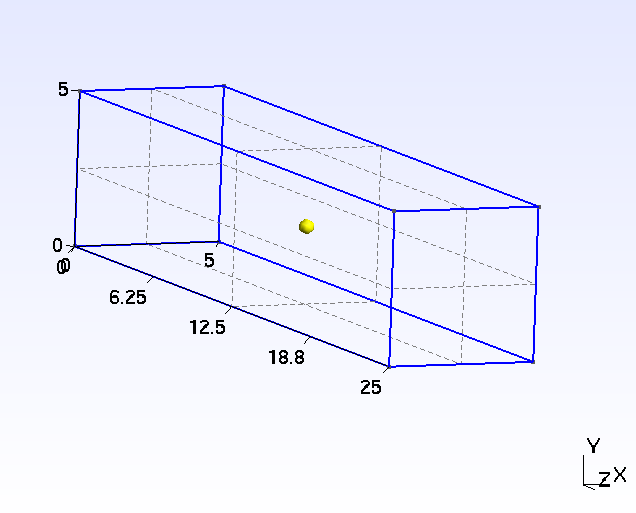
Figure 5.1: Rectangular block of size $5\times 5\times 25$ with a plane interface at $z=12.5$

In order to test the implementation of Nitsche’s method, a simple rectangular block with an interface in between was used.The block was tested under conditions of jump in displacement at the interface as well as a prescribed Dirichlet conditions on both sides of the interface. The following conditions were assumed :

$$E=205\times 10{}^{3}\mbox{ Pa}$$

$$\nu=0.3$$

$$L=25\mbox{ mm}$$

$$f=0\mbox{ N}\mbox{ in }\Omega$$

$$u_{z}(z=0)=u_{z}(z=25)=0\mbox{ mm}$$

$$u_{x}(x=0)=0\mbox{ mm}$$

$$u_{y}(y=0)=0\mbox{ mm}$$

1. For the case of jump in displacement

   $$\bar{\mbox{i}}=\left[\left[u_{z}(z=12.5)\right]\right]=3\times 10^{-6}\mbox{ m}$$

   $$\bar{\mbox{j}}=\left[\left[\sigma(z=12.5)\right]\right].\mbox{n}=0\mbox{ Pa}$$

2. For the case of Dirichlet condition

   $$g^{+}=u_{z}^{+}(z=12.5)=1.5\times 10^{-6}\mbox{ m}$$

   $$g^{-}=u_{z}^{-}(z=12.5)=-1.5\times 10^{-6}\mbox{ m}$$

It can be noted that both conditions will generate the same output. Due to the symmetric nature of the problem, we consider $g^{+}=g^{-}=g$. Analytically, the solution for the above problem is:

$$\sigma_{zz}=-\frac{2Eg}{L}\mbox{ in }\Omega$$ (5.1)

$$u_{x}=\frac{2\nu gx}{L}$$ (5.2)

$$u_{y}=\frac{2\nu gy}{L}$$ (5.3)

$$u_{z}=-\frac{2gz}{L}\mbox{ in }\Omega^{-}$$ (5.4)

$$u_{z}=-\frac{2gz}{L}+2g\mbox{ in }\Omega^{+}$$ (5.5)

The above problem was tested with both Nitsche’s method and the penalization method with varying penalization parameter. The solutions obtained were then compared to the analytical solution in terms of error in energy norm and displacement norm in $L_{2}$.

The solution is shown in Figure 5.2 imprinted on the hexahedral mesh. If we look at the error norms, both Dirichlet and jump conditions have similar behavior, thus signifying the equivalence of the two methods for equivalent boundary conditions. We see that for penalization method, the solution tends to converge at higher penalization parameter while for Nitsche’s method, we obtain good results even at very low stabilization parameter and in fact, the machine error adds up at higher parameter (Figures 5.3 and 5.4), resulting in higher error, even for Nitsche’s method!

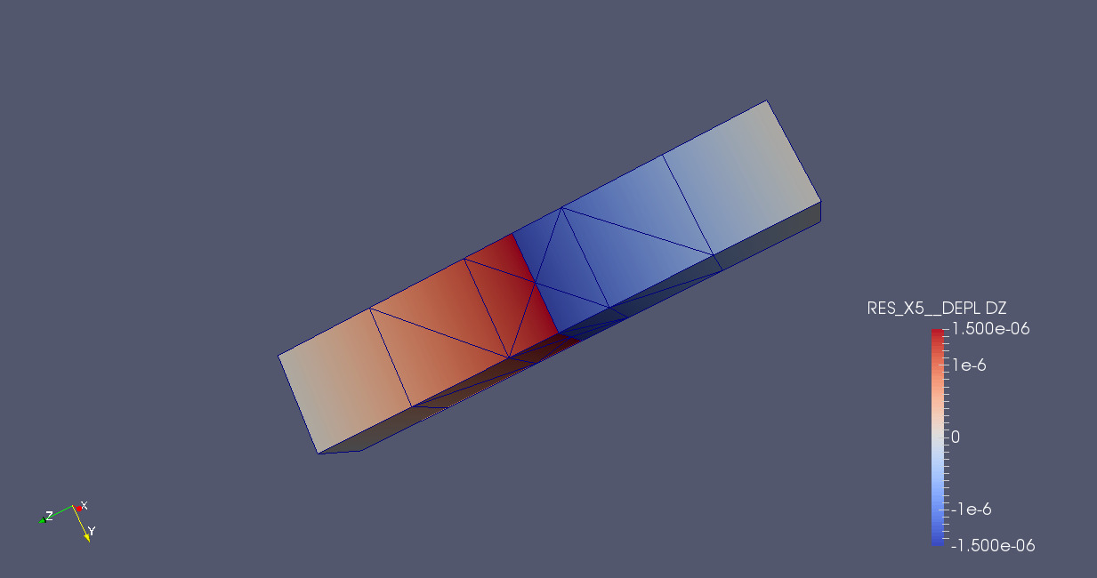
Figure 5.2: the solution as obtained in Code Aster after analyzing a problem of jump type using non-linear Newton iterations.

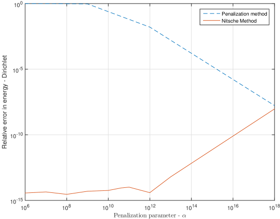
Figure 5.3: Relative energy norm error for Dirichlet conditions and the study of their variation with change in stabilization parameter in Nitsche’s and penalization methods.

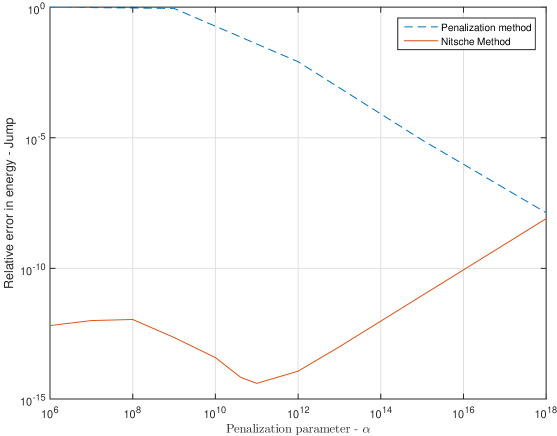
Figure 5.4: Relative energy norm error for Jump conditions and the study of their variation with change in stabilization parameter in Nitsche’s and penalization methods.

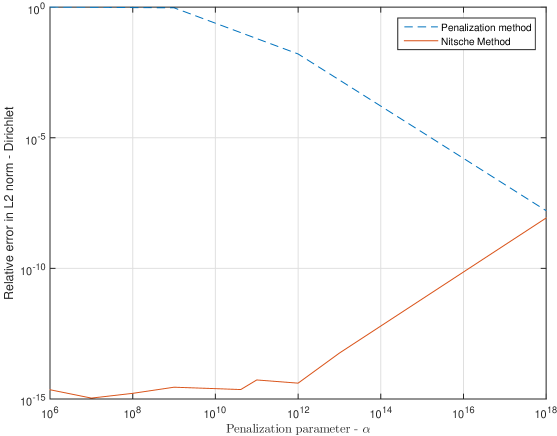
Figure 5.5: Relative L2 norm error for Dirichlet conditions and the study of their variation with change in stabilization parameter in Nitsche’s and penalization methods.

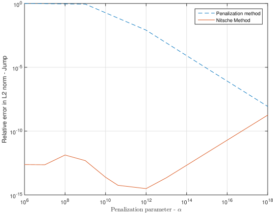
Figure 5.6: Relative L2 norm error for Jump conditions and the study of their variation with change in stabilization parameter in Nitsche’s and penalization methods.

5.3 Circular Inclusion problem

In this two-dimensional bi-material test case, a weak discontinuity is present, and the displacement field is continuous with discontinuous stresses and strains.[8, 11] Inside a circular plate of radius b, whose material is defines by $E_{1}=1$ and $\nu_{1}=0.25$, a circular inclusion with radius $a$ of different material with $E_{2}=10$ and $\nu=0.3$ is considered. The loading of the structure results from a linear displacement of the outer boundary: $u_{r}\left(b,\theta\right)=r$ and $u_{\theta}\left(b,\theta\right)=0$. The situation is depicted in figure (5.7). The exact solution can be found in [12].

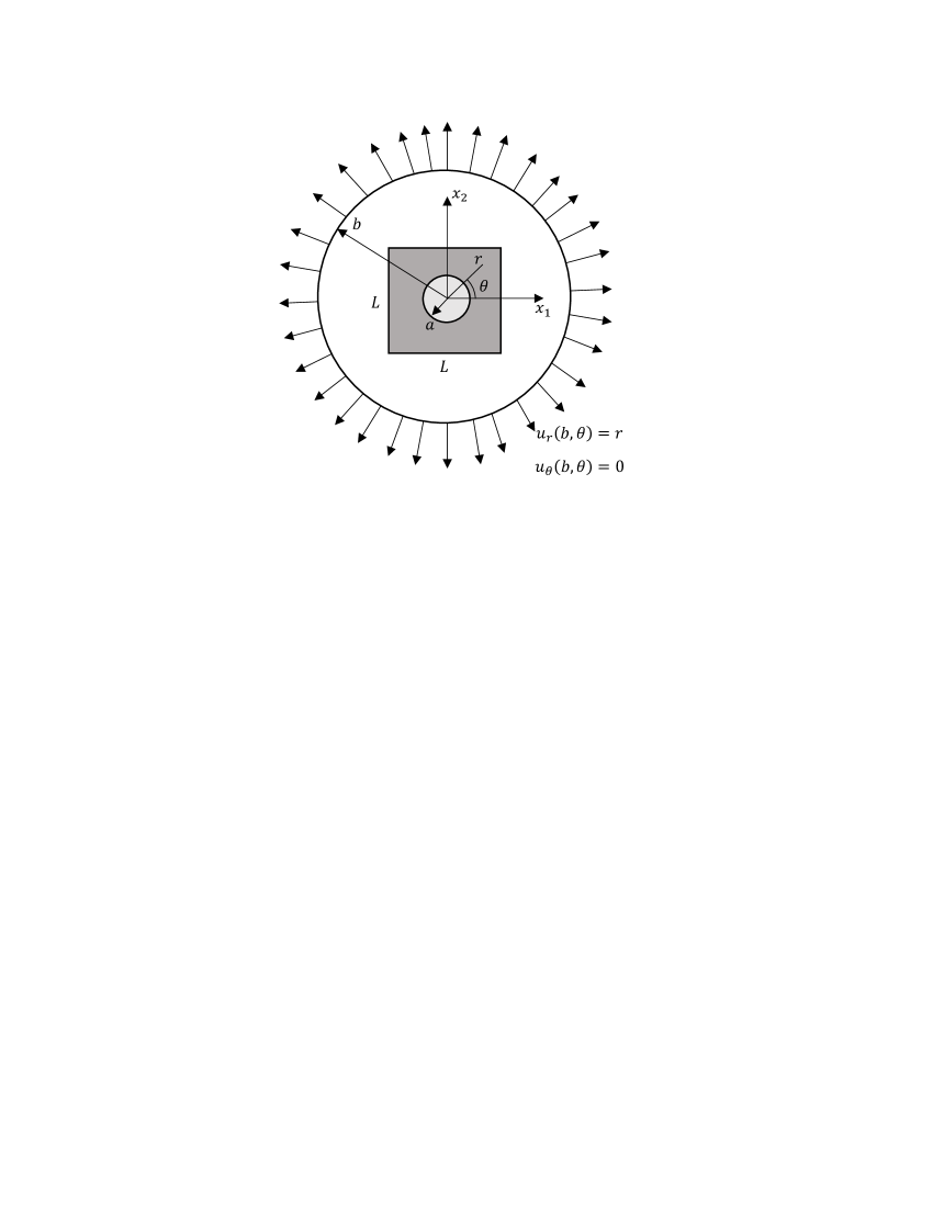
Figure 5.7: Problem statement of the circular inclusion problem (the gray area is the numerical domain)

The stresses are given as:

$$\sigma_{rr}\left(r,\theta\right)=2\mu\varepsilon_{rr}+\lambda\left(\varepsilon_{rr}+\varepsilon_{\theta\theta}\right)$$ (5.6)

$$\sigma_{\theta\theta}\left(r,\theta\right)=2\mu\varepsilon_{\theta\theta}+\lambda\left(\varepsilon_{rr}+\varepsilon_{\theta\theta}\right)$$ (5.7)

where the Lamé constants $\lambda$ and $\mu$ have to be replaced by the appropriate values for the corresponding area, respectively. The strains are:

$$\varepsilon_{rr}\left(r,\theta\right)=\begin{cases}\left(1-\frac{b^{2}}{a^{2}}\right)\alpha+\frac{b^{2}}{a^{2}},&0\leq r\leq a\\ \left(1+\frac{b^{2}}{r^{2}}\right)\alpha-\frac{b^{2}}{r^{2}},&a\leq r\leq b\end{cases}$$ (5.8)

$$\varepsilon_{\theta\theta}\left(r,\theta\right)=\begin{cases}\left(1-\frac{b^{2}}{a^{2}}\right)\alpha+\frac{b^{2}}{a^{2}},&0\leq r\leq a\\ \left(1+\frac{b^{2}}{r^{2}}\right)\alpha-\frac{b^{2}}{r^{2}},&a\leq r\leq b\end{cases}$$ (5.9)

and the displacements:

$$u_{r}\left(r,\theta\right)=\begin{cases}\left[\left(1-\frac{b^{2}}{a^{2}}\right)\alpha+\frac{b^{2}}{a^{2}}\right]r,&0\leq r\leq a\\ \left(r-\frac{b^{2}}{r^{2}}\right)\alpha+\frac{b^{2}}{r},&a\leq r\leq b\end{cases}$$ (5.10)

$$u_{\theta}\left(r,\theta\right)=0$$ (5.11)

The parameter $\alpha$ involved in these definitions is:

$$\alpha=\frac{\left(\lambda_{1}+\mu_{1}+\mu_{2}\right)b^{2}}{\left(\lambda_{2}+\mu_{2}\right)a^{2}+\left(\lambda_{1}+\mu_{1}\right)\left(b^{2}-a^{2}\right)+\mu_{2}b^{2}}$$ (5.12)

For the numerical model, the domain is a square of size $L\times L$ with $L=2$, the outer radius is chosen to be $b=2$ and the inner radius $a=0.4$. The exact stresses are prescribed along the boundaries of the square domain, and displacements are prescribed as:

$$u_{1}\left(0,\pm 1\right)=0$$

and:

$$u_{2}\left(\pm 1,0\right)=0$$

Plane strain conditions are assumed. Results are obtained for different methods, Nitsche’s method, penalty method and non-linear method with Lagrange multipliers. A set of displacement and stress on gauss points plots have been presented in figures 5.8 to 5.12. The interface is embedded into the mesh and Code Aster divides every element cut by the interface into sub-elements. The elements adjacent to the ones cut by interface are also enriched. (Figure 5.10). The displacement plot shows a continuous change of the magnitude in both the axis(figure 5.11), while the stress plot shows the discontinuous stress in the two domains.

We compare the error norms by considering linear irregular, linear regular, quadratic irregular, qudratic regular and triangular irregular elements. Note that in quadratic elements, the shape functions assume a quadratic nature. (Figures 5.13 and 5.14) The convergence order is the highest for a structured grid with quadratic shape functions. This is obvious as better approximation is obtained with higher order of polynomial. On comparison with other methods like penalty and lagrange multipliers (figures 5.16 and5.17), we see that Nitsche’s method has slightly better convergence than penalty method. But we have seen from the previous example that we need to prescribe very high penalization parameter to obtain this resulting in higher conditioning of the system. Nitsche’s method is competitive on comparison to Lagrange method but comes free of additional degree of freedom associated with Lagrange multipliers.

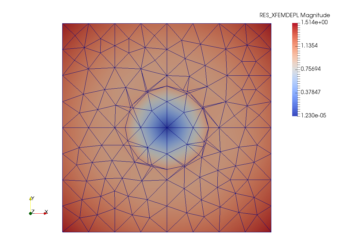
Figure 5.8: Circular inclusion problem solution on an irregular grid of size $h=0.2$. Notice how the element is divided into subelements at the interface.

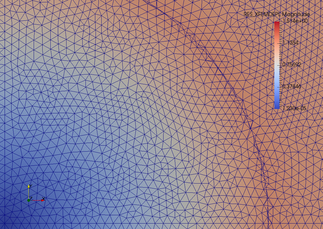
Figure 5.9: Circular inclusion problem solution on an irregular grid of size $h=0.0125$. In this close up view the effect of level set on the mesh and the solution can be seen.

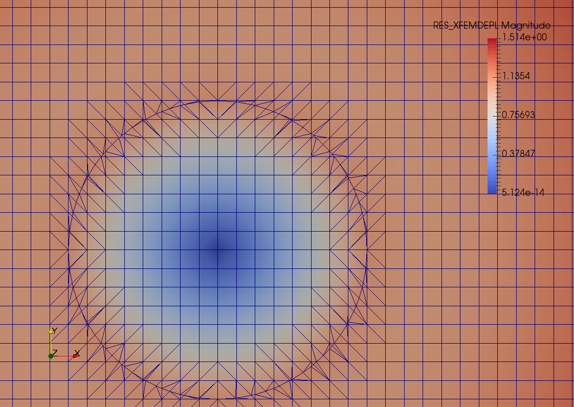
Figure 5.10: Circular inclusion problem solution on an regular grid of size $h=0.05$. The enrichment is extended to an element beyond the interface in both sides.

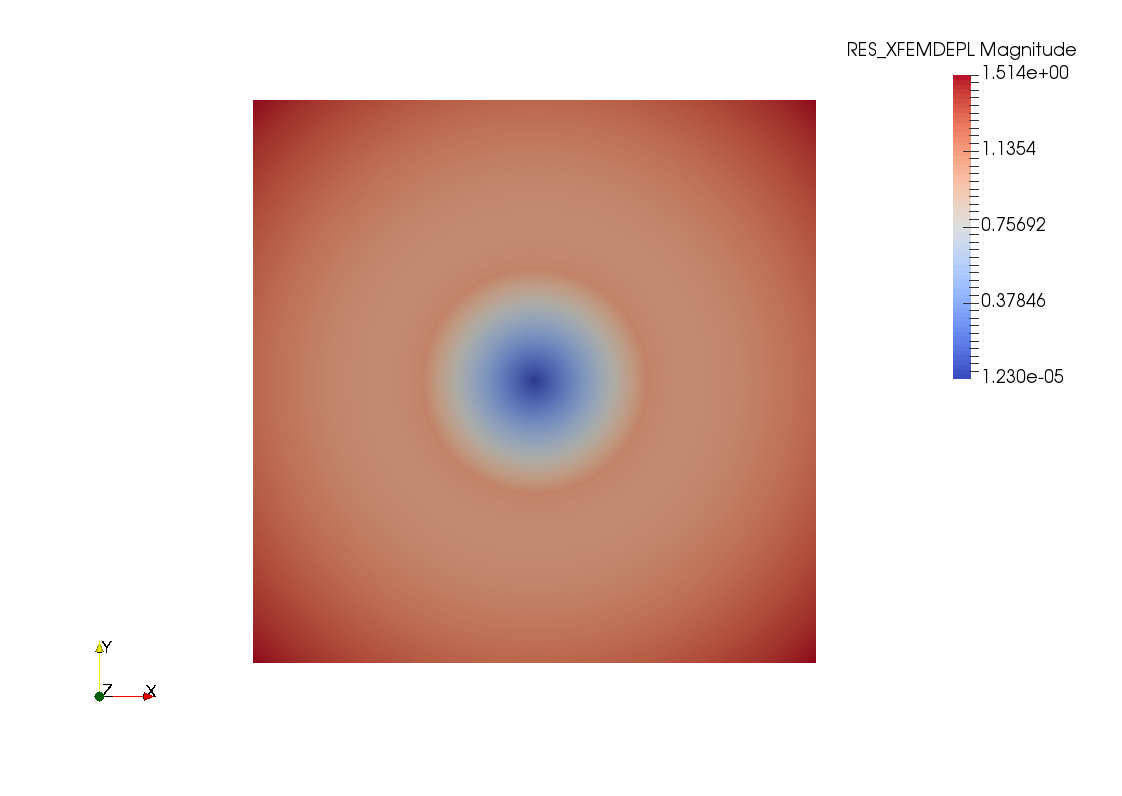
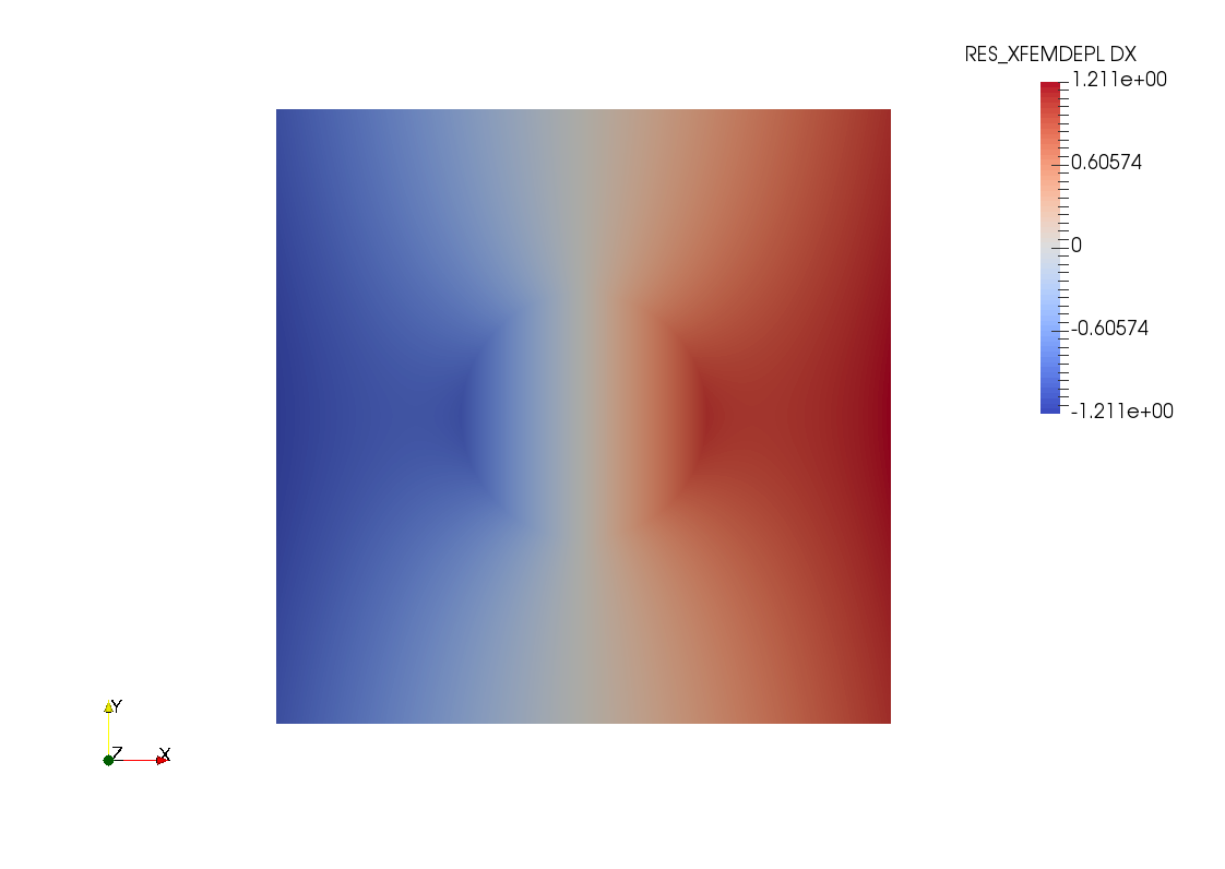
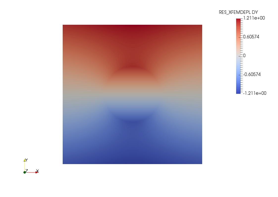
Figure 5.11: Circular inclusion problem solution on an regular grid of size $h=0.0125$. Magnitude of the displacement solution on the entire domain and its variation with respect to x and y direction.

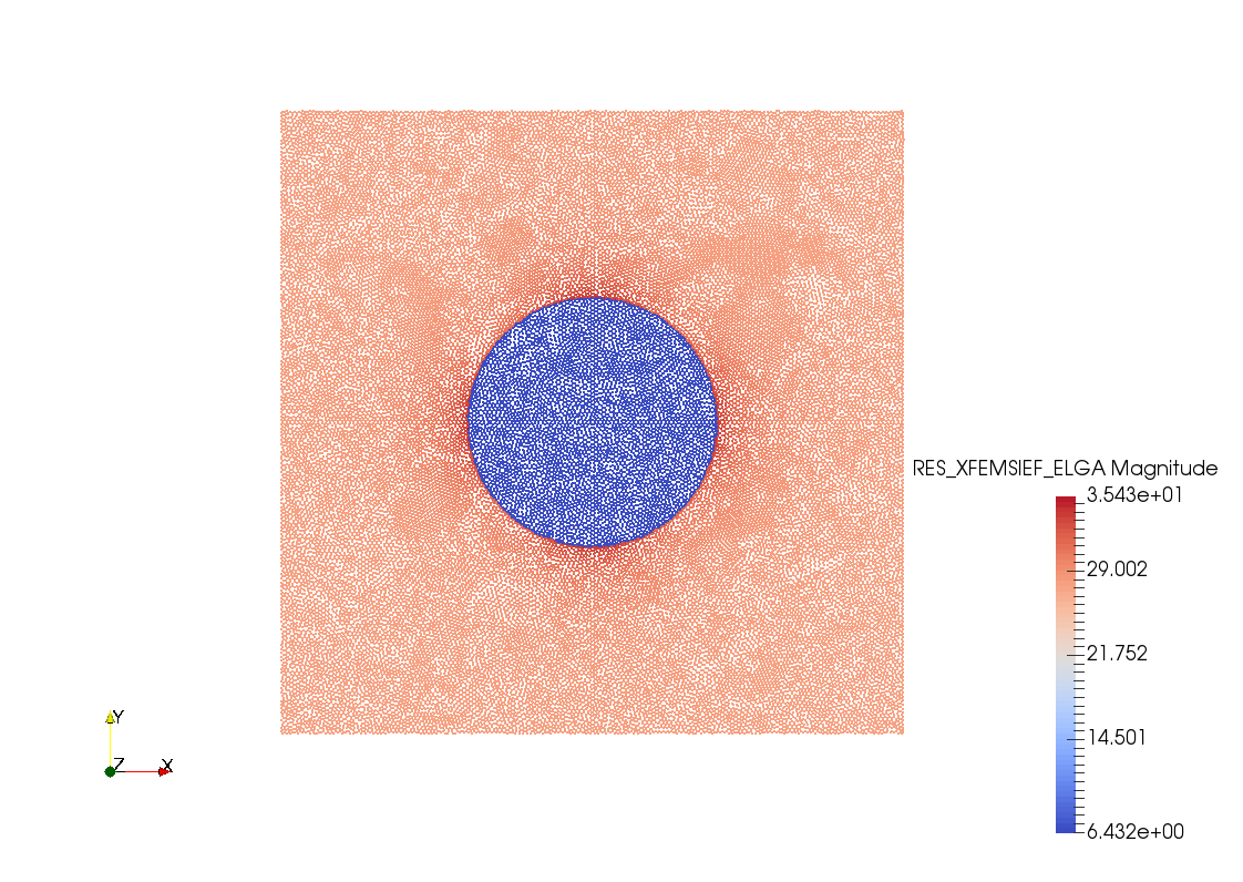
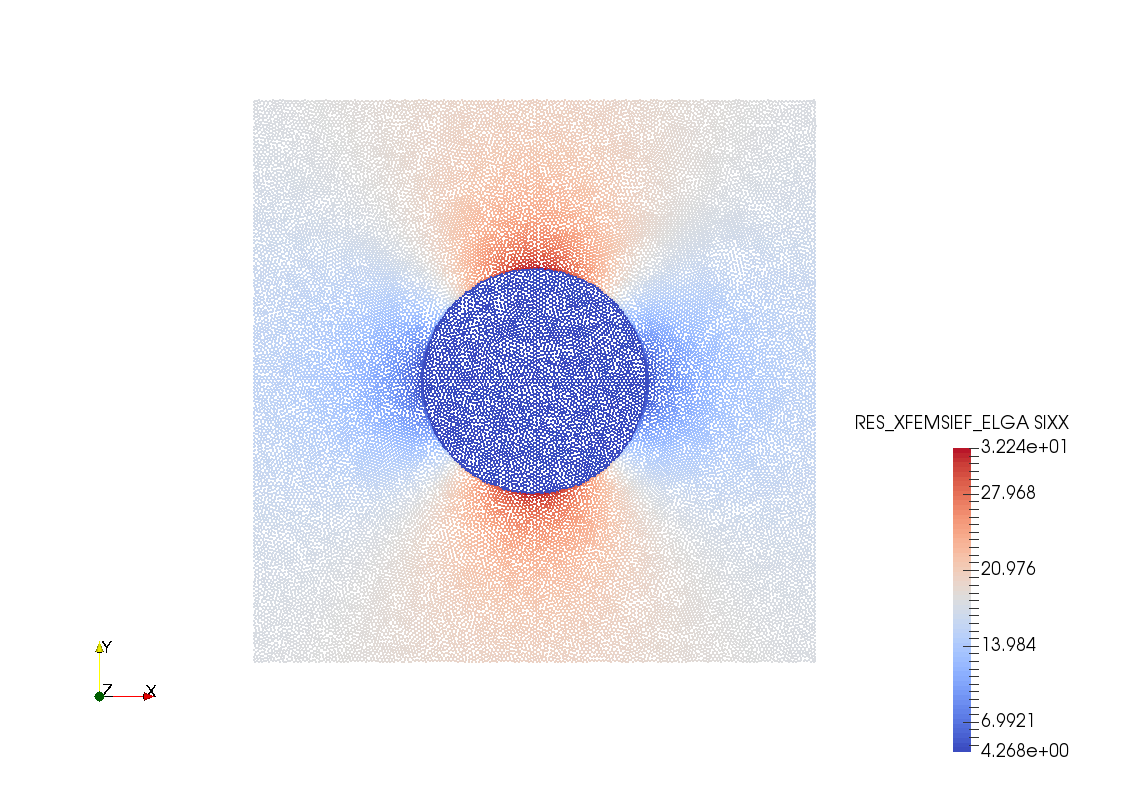
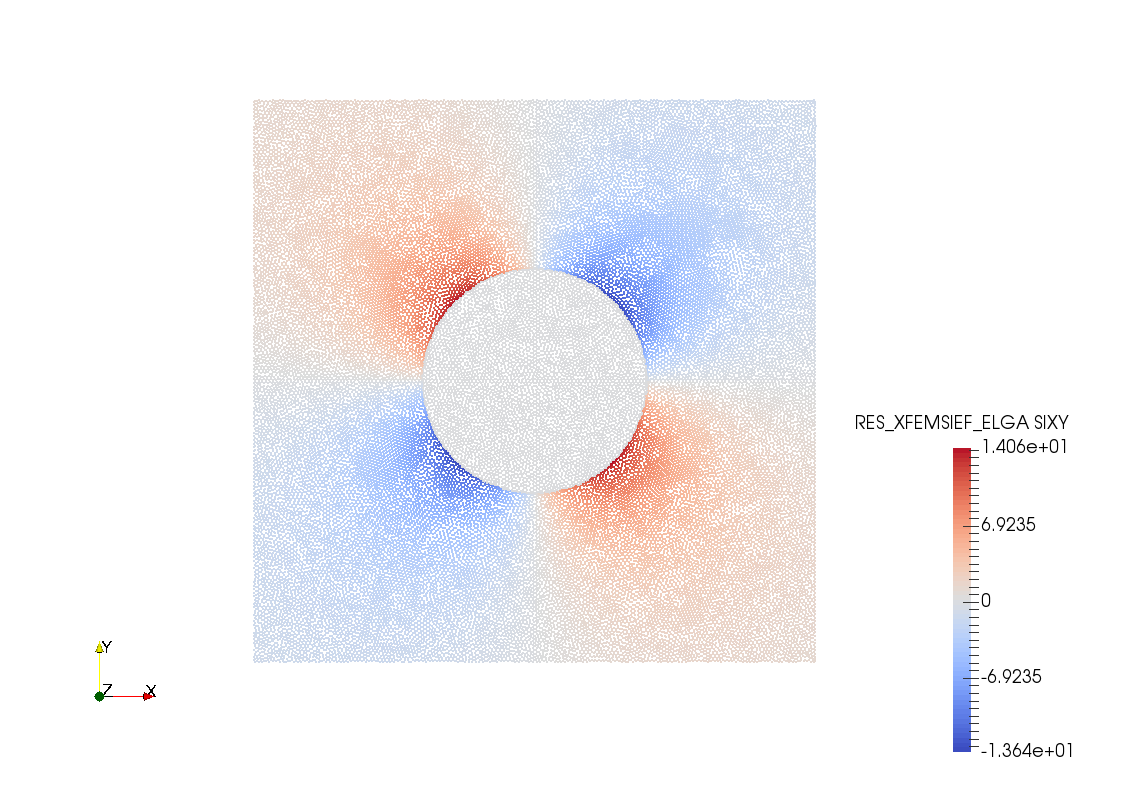
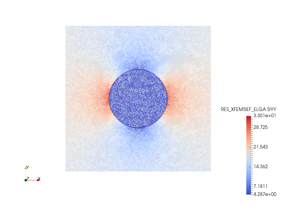
Figure 5.12: Circular inclusion problem solution on an regular grid of size $h=0.0125$. Solution of the discontinuous stresses in the domain

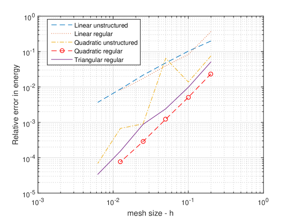
Figure 5.13: Relative energy norm error for the circular inclusion problem - comparison with various grids and order of the shape functions.

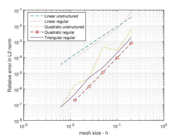
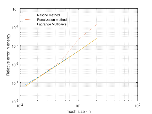
Figure 5.14: Relative L2 norm error for the circular inclusion problem - comparison with various grids and order of the shape functions.

Figure 5.15: Relative energy norm error for the circular inclusion problem - comparison between the three methods on a regular quadratic grid.

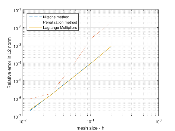
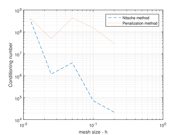
Figure 5.16: Relative L2 norm error for the circular inclusion problem - comparison between the three methods on a regular quadratic grid.

Figure 5.17: Condition number comparison for the circular inclusion problem between Nitsche’s method and penalty method.

6 Conclusion and future scope

As can be seen from this work, Nitsche’s method was succesfully implemented in Code-Aster using X-FEM discretization with shifted basis enrichment. We have seen that this method is better in terms of relative error as compared to standard penalty methods as well as relieves us from calculating a ’free’ detrimental penalization or stabilization parameter, and instead focuses on domain dependant parameters. We calculate these parameters based on numerical analysis, insisting on the coercivity of the bilinear form. Also the method is better than Lagrange multipliers method as it can calculate the solution in the same computational range but without any extra degree of freedom that is associated with Lagrange method.

With the help of simple yet effective problems we have brought forth the advantages of a method that can capture solutions whiile enforcing internal constraints. Coupled with X-FEM, discontinuous enrichment of finite element basis functions allows the construction of a solution space that takes into account discontinuities at interfaces without the disadvantage of needing to grid the interfaces.The method is straightforward to implement, requiring only the modifications of element stiffness routines of elements intersected by the interface. With the introduction of a shifted basis enrichment we get increased convergence.

One of the next step would be to extend the method on tips and cracks with internal endings. This can come in handy especially when the two opposing lips of a crack are constrained. Also, this can be clubbed with Nitsche’s method in contact and can help analyse models with constaint on one side and contact friction on the other with vastly differing material properties. Also this method can be extended to dynamic problems, like fluid flow or the seismic activities.

Appendix

Appendix A Stabilization parameter

The stabilization or penalization parameter, $\alpha$, is defined such that the appropriate bilinear form is coercive. We use the local approach here, which offers added simplicity and efficiency.[3, 6, 7] Referring back to the discrete bilinear form containing both bulk and interfacial components, $a_{i}\left(\boldsymbol{u}^{h},\boldsymbol{v}^{h}\right)$ we further define an ’energy’ norm:

$$\left|\left|\boldsymbol{v}^{h}\right|\right|_{E}^{2}=\left(\varepsilon\left(\boldsymbol{v}\right),\sigma\left(\boldsymbol{v}\right)\right)$$ (A.1)

Here, $\left(\centerdot,\centerdot\right)$ is the $L_{2}$ inner product. The duality pairing $\left\langle\centerdot,\centerdot\right\rangle$ denotes integration along the interface.

Dirichlet condition.

Considering this problem as two ’one-sided’ problems, we consider one domain for simplicity, $\Omega^{-}$. We make use of the generalized inverse estimate and there exists a configuration dependent constant $C_{1}$, to assert coercivity, such that

$$\left|\left|\sigma\left(\boldsymbol{v}^{h}\right)_{,n}\right|\right|_{\Gamma_{e}^{*}}\leq C_{1}\left|\left|\boldsymbol{v}^{h}\right|\right|_{\Omega_{e}^{-},E}$$ (A.2)

The gradient is constant within the element and the normal derivative is constant along the interface, helping us obtain a lower obtain for $C_{1}$. For the case of linear triangular element on a linear isotropic element

$$\left|\left|\sigma\left(\boldsymbol{v}^{h}\right)_{,n}\right|\right|_{\Gamma_{e}^{*}}^{2}=L_{s}\left(\sigma\left(\boldsymbol{v}^{h}\right).n\right)^{2}\leq L_{s}E^{2}\left|\varepsilon\left(\boldsymbol{v}^{h}\right)\right|^{2}$$ (A.3)

$$\left|\left|\boldsymbol{v}^{h}\right|\right|_{\Omega_{e}^{-},E}^{2}=A^{-}E\left|\varepsilon\left(\boldsymbol{v}^{h}\right)\right|^{2}$$ (A.4)

with $L_{s}=\mbox{meas}\left(\Gamma_{e}^{*}\right)$ and $A^{-}=\mbox{meas}\left(\Omega_{e}^{-}\right)$. Thus we have

$$C_{1}^{2}\geq EL_{s}/A^{-}$$

Similarly for the case of linear tetrahedron, we can write

$$C_{1}^{2}\geq EA_{s}/V^{-}$$

with $A_{s}=\mbox{meas}\left(\Gamma_{e}^{*}\right)$ and $V^{-}=\mbox{meas}\left(\Omega_{e}^{-}\right)$. Utilizing the lowest estimate for $C_{1}$ we can use, for a given element

$$\alpha_{e}=2C_{1}^{2}$$ (A.5)

which provides coercivity of the bilinear form on (3.9),

$$a\left(v^{h},v^{h}\right)_{e} = \int_{\Omega}\varepsilon(v)\sigma\mathrm{d\Omega}-\int_{\mathcal{S}}v^{-}\left(\sigma^{-}\right).\mathbf{n}\mathrm{d}\mathrm{\Gamma}-\int_{\mathcal{S}}v^{-}\left(\sigma{}^{-}\right).\mathbf{n}\mathrm{d}\mathrm{\Gamma}+\int_{\mathcal{S}}v^{-}\alpha_{e}^{-}v^{-}\mathrm{d}\mathrm{\Gamma}$$ (A.6)

$$= \left|\left|v^{h}\right|\right|_{\Omega^{-},E}^{2}-2\left\langle\sigma^{-}\left(v^{h}\right){}_{,n},v^{h}\right\rangle_{\Gamma^{*}}+\alpha_{e}\left|\left|v^{h}\right|\right|_{\Gamma^{*}}^{2}$$

Young’s inequality (also Peter-Paul inequality) with $\epsilon>0$, gives

$$2\left\langle\sigma^{-}\left(v^{h}\right){}_{,n},v^{h}\right\rangle_{\Gamma^{*}}\leq\epsilon\left|\left|\sigma^{-}\left(v^{h}\right){}_{,n}\right|\right|_{\Gamma^{*}}^{2}+\frac{1}{\epsilon}\left|\left|v^{h}\right|\right|_{\Gamma^{*}}^{2}$$ (A.7)

Thus, from the definition of unit vector, we have the inequality

$$a\left(v^{h},v^{h}\right)_{e} \geq \left|\left|v^{h}\right|\right|_{\Omega^{-},E}^{2}-\epsilon\left|\left|\sigma^{-}\left(v^{h}\right){}_{,n}\right|\right|_{\Gamma^{*}}^{2}+\left(\alpha_{e}-\frac{1}{\epsilon}\right)\left|\left|v^{h}\right|\right|_{\Gamma^{*}}^{2}$$ (A.8)

$$\geq \left(1-\epsilon C_{1}^{2}\right)\left|\left|v^{h}\right|\right|_{\Omega^{-},E}^{2}+\left(\alpha_{e}-\frac{1}{\epsilon}\right)\left|\left|v^{h}\right|\right|_{\Gamma^{*}}^{2}$$ (A.9)

By using $\epsilon=1/\alpha_{e}$ and $\alpha_{e}=2C_{1}^{2}$ we get

$$a\left(v^{h},v^{h}\right)_{e}\geq\frac{1}{2}\left|\left|v^{h}\right|\right|_{\Omega^{-},E}^{2}$$ (A.10)

We can see that coercivity is ensured with any choice of $\alpha_{e}\geq 1/\epsilon\geq C_{1}^{2}$ while (A.5) provides good performance in computation.

Jump condition.

The generalized inverse estimate (A.2) is extended to account for the average flux

$$\left|\left|\left\langle\sigma\left(\boldsymbol{v}^{h}\right)_{,n}\right\rangle\right|\right|_{\Gamma^{*}}\leq C_{1}\left|\left|\boldsymbol{v}^{h}\right|\right|_{\Omega,E}$$ (A.11)

in terms of energy norm (A.1).

For a linear triangular element, the gradient is piecewise constant within the element. Assuming isotropic material, $E$ is also piecewise constant within each element, the mean flux is constant along the interface; thus,

$$\left|\left|\left\langle\sigma\left(\boldsymbol{v}^{h}\right)_{,n}\right\rangle\right|\right|_{\Gamma^{*}}^{2}=L_{s}\left\langle\sigma\left(\boldsymbol{v}^{h}\right)_{,n}\right\rangle^{2}$$ (A.12)

$$\left|\left|\boldsymbol{v}^{h}\right|\right|_{\Omega,E}^{2}=A^{-}E^{-}\left|\varepsilon\left(\boldsymbol{v}^{h-}\right)\right|^{2}+A^{+}E^{+}\left|\varepsilon\left(\boldsymbol{v}^{h+}\right)\right|^{2}$$ (A.13)

For the average flux

$$\left\langle\sigma\left(\boldsymbol{v}^{h}\right)_{,n}\right\rangle^{2} = \frac{1}{4}\left(\sigma\left(\boldsymbol{v}^{h^{+}}\right).n+\sigma\left(\boldsymbol{v}^{h^{-}}\right).n\right)^{2}$$

$$\left(\sigma\left(\boldsymbol{v}^{h^{+}}\right).n+\sigma\left(\boldsymbol{v}^{h^{-}}\right).n\right) \leq \left(1+\epsilon\right)\left(\sigma\left(\boldsymbol{v}^{h^{-}}\right).n\right)^{2}+\left(1+\frac{1}{\epsilon}\right)\left(\sigma\left(\boldsymbol{v}^{h+}\right).n\right)^{2}\mbox{ }\forall\epsilon>0$$ (A.14)

This follows from Young’s inequality. By selecting $\epsilon=E^{+}A^{-}/E^{-}A^{+}$ we get

$$\left\langle\sigma\left(\boldsymbol{v}^{h}\right)_{,n}\right\rangle^{2} \leq \left(1+\frac{E^{+}A^{-}}{E^{-}A^{+}}\right)\left(E^{-}\right)^{2}\left|\varepsilon\left(\boldsymbol{v}^{h^{-}}\right)\right|^{2}+\left(1+\frac{E^{-}A^{+}}{E^{+}A^{-}}\right)\left(E^{+}\right)^{2}\left|\varepsilon\left(\boldsymbol{v}^{h+}\right)\right|^{2}$$ (A.15)

$$= \left(\frac{E^{-}}{A^{-}}+\frac{E^{+}}{A^{+}}\right)\left(A^{-}E^{-}\left|\varepsilon\left(\boldsymbol{v}^{h^{+}}\right)\right|^{2}+A^{+}E^{+}\left|\varepsilon\left(\boldsymbol{v}^{h^{-}}\right)\right|^{2}\right)$$ (A.16)

As can be seen, the generalized inverse estimate is satisfied for

$$C_{1}^{2}\geq\frac{L_{s}}{4}\left(\frac{E^{-}}{A^{-}}+\frac{E^{+}}{A^{+}}\right)$$

Similarly, for the linear tetrahedron,

$$C_{1}^{2}\geq\frac{A_{s}}{4}\left(\frac{E^{-}}{V^{-}}+\frac{E^{+}}{V^{+}}\right)$$

Following what has been done from (A.6) to (A.10),

$$a\left(v^{h},v^{h}\right)_{e} = \int_{\Omega}\varepsilon(v)\sigma\mathrm{d\Omega}-\int_{\mathcal{S}}[[v]]<\sigma>.\mathbf{n}\mathrm{d\Gamma}-\int_{\mathcal{S}}[[v]]<\sigma>.\mathbf{n}\mathrm{d\Gamma}+\int_{\mathcal{S}}[[v]]\alpha[[v]]\mathrm{d\Gamma}$$ (A.17)

$$= \left|\left|v^{h}\right|\right|_{\Omega,E}^{2}-2\left\langle\left\langle\sigma\left(v^{h}\right){}_{,n}\right\rangle,\left[\left[v^{h}\right]\right]\right\rangle_{\Gamma^{*}}+\alpha_{e}\left|\left|\left[\left[v^{h}\right]\right]\right|\right|_{\Gamma^{*}}^{2}$$

$$\geq \left|\left|v^{h}\right|\right|_{\Omega,E}^{2}-\epsilon\left|\left|\left\langle\sigma\left(v^{h}\right){}_{,n}\right\rangle\right|\right|+\left(\alpha_{e}-\frac{1}{\epsilon}\right)\left|\left|\left[\left[v^{h}\right]\right]\right|\right|_{\Gamma^{*}}^{2}\mbox{ }\forall\epsilon>0$$ (A.18)

$$\geq \left(1-\epsilon C_{1}^{2}\right)\left|\left|v^{h}\right|\right|_{\Omega,E}^{2}+\left(\alpha_{e}-\frac{1}{\epsilon}\right)\left|\left|\left[\left[v^{h}\right]\right]\right|\right|_{\Gamma^{*}}^{2}$$ (A.19)

$$\geq \frac{1}{2}\left|\left|v^{h}\right|\right|_{\Omega,E}^{2}$$ (A.20)

This gives the same coercivity assurance as in (A.10). Thus the stabilization parameter can be chosen according to (A.5).

Weighted parameters

Similar to what was done in the previous section, we have, using Cauchy-Schwartz inequality

$$a\left(v^{h},v^{h}\right)_{e} = \left|\left|v^{h}\right|\right|_{\Omega,E}^{2}-2\left\langle\left\langle\sigma\left(v^{h}\right){}_{,n}\right\rangle_{\gamma},\left[\left[v^{h}\right]\right]\right\rangle_{\Gamma^{*}}+\alpha_{e}\left|\left|\left[\left[v^{h}\right]\right]\right|\right|_{\Gamma^{*}}^{2}$$

$$\geq \left|\left|v^{h}\right|\right|_{\Omega,E}^{2}+\alpha_{e}\left|\left|\left[\left[v^{h}\right]\right]\right|\right|_{\Gamma^{*}}^{2}-2\left|\left|\left[\left[v^{h}\right]\right]\right|\right|_{\Gamma^{*}}\left|\left|\left\langle\sigma\left(v^{h}\right)\right\rangle_{\gamma}.n\right|\right|_{\Gamma^{*}}$$

$$\geq \left(\left|\left|v^{h}\right|\right|_{\Omega,E}-C_{1}\left|\left|\left[\left[v^{h}\right]\right]\right|\right|_{\Gamma^{*}}\right)^{2}+\left(\alpha_{e}-C_{1}^{2}\right)\left|\left|\left[\left[v^{h}\right]\right]\right|\right|_{\Gamma^{*}}$$

with $\left|\left|\left\langle\sigma\left(v^{h}\right)\right\rangle_{\gamma}.n\right|\right|_{\Gamma^{*}}\leq C_{1}\left|\left|v^{h}\right|\right|_{\Omega,E}$. We use generalized inverse estimate, to find the lower bound for $C_{1}^{2}$.

For a linear triangular element, the gradient is piecewise constant within the element. Assuming isotropic material, $E$ is also piecewise constant within each element, the mean flux is constant along the interface; thus,

$$\left|\left|\boldsymbol{v}^{h}\right|\right|_{\Omega,E}^{2}=A^{-}E^{-}\left|\varepsilon\left(\boldsymbol{v}^{h-}\right)\right|^{2}+A^{+}E^{+}\left|\varepsilon\left(\boldsymbol{v}^{h+}\right)\right|^{2}$$ (A.21)

$$\left|\left|\left\langle\sigma\left(\boldsymbol{v}^{h}\right)_{,n}\right\rangle_{\gamma}\right|\right|_{\Gamma^{*}}^{2} = L_{s}\left\langle\sigma\left(\boldsymbol{v}^{h}\right)_{,n}\right\rangle_{\gamma}^{2}$$ (A.22)

$$= L_{s}\left(\gamma_{e}E\left|\varepsilon\left(\boldsymbol{v}^{h+}\right)\right|.n+\left(1-\gamma_{e}\right)E\left|\varepsilon\left(\boldsymbol{v}^{h-}\right)\right|.n\right)^{2}$$ (A.23)

$$\leq L_{s}\left(\left(\gamma_{e}E\left|\varepsilon\left(\boldsymbol{v}^{h+}\right)\right|\right)^{2}\left(1+\epsilon\right)+\left(\left(1-\gamma_{e}\right)E\left|\varepsilon\left(\boldsymbol{v}^{h-}\right)\right|\right)^{2}\left(1+\frac{1}{\epsilon}\right)\right)$$ (A.24)

from Young’s inequality. By selecting $\epsilon=E^{+}A^{-}\gamma_{e}^{2}/E^{-}A^{+}\left(1-\gamma_{e}\right)^{2}$ we get

$$\left\langle\sigma\left(\boldsymbol{v}^{h}\right).n\right\rangle_{\Gamma^{*}}^{2} \leq \left(1+\frac{E^{+}A^{-}\gamma_{e}^{2}}{E^{-}A^{+}\left(1-\gamma_{e}\right)^{2}}\right)\left(\left(1-\gamma_{e}\right)E^{-}\left|\varepsilon\left(\boldsymbol{v}^{h^{-}}\right)\right|\right)^{2}+\left(1+\frac{E^{-}A^{+}\left(1-\gamma_{e}\right)^{2}}{E^{+}A^{-}\gamma_{e}^{2}}\right)\left(\gamma_{e}E^{+}\left|\varepsilon\left(\boldsymbol{v}^{h+}\right)\right|\right)^{2}$$ (A.25)

$$= \left(\frac{\left(1-\gamma_{e}\right)^{2}E^{-}}{A^{-}}+\frac{\gamma_{e}^{2}E^{+}}{A^{+}}\right)\left(A^{-}E^{-}\left|\varepsilon\left(\boldsymbol{v}^{h^{-}}\right)\right|^{2}+A^{+}E^{+}\left|\varepsilon\left(\boldsymbol{v}^{h^{+}}\right)\right|^{2}\right)$$

As can be seen, the generalized inverse estimate is satisfied for

$$C_{1}^{2}\geq L_{s}\left(\frac{E^{-}\left(1-\gamma_{e}\right)^{2}}{A^{-}}+\frac{E^{+}\gamma_{e}^{2}}{A^{+}}\right)$$

Similarly, for the linear tetrahedron,

$$C_{1}^{2}\geq A_{s}\left(\frac{E^{-}\left(1-\gamma_{e}\right)^{2}}{V^{-}}+\frac{E^{+}\gamma_{e}^{2}}{V^{+}}\right)$$

If we use the smart choice for $\gamma_{e}$ from (3.405), then we get

$$C_{1}^{2}=\frac{L_{s}}{\left(\frac{A^{-}}{E^{-}}+\frac{A^{+}}{E^{+}}\right)}$$ (A.26)

which helps us avoid numerical issues that creep up due to conforming meshes from classical Nitsche’s values for $C_{1}$. Recalling (A.5), the stabilization parameter for weighted algorithm is

$$\alpha_{e}=2C_{1}^{2}$$

References

- [1] Juntunen, Mika, and Rolf Stenberg. “Nitsche’s’s method for general boundary conditions.” Mathematics of computation 78.267 (2009): 1353-1374.
- [2] Sanders, D. Jessica, John E. Dolbow and Tod A. Laursen. “On methods for stabilizing constraints over enriched interfaces in elasticity.” International journal for numerical methods in engineering 78 (2009): 1009-1036
- [3] Dolbow, John, and Isaac Harari. “An efficient finite element method for embedded interface problems.” International journal for numerical methods in engineering 78 (2009): 229-252.
- [4] Dolbow, John. “Constraints on Embedded Interfaces I.” Numerical Analysis Summer School 2014
- [5] Annavarapu, Chandrasekhar, Martin Hautefeuille, and John E. Dolbow. “A robust Nitsche’s’s formulation for interface problems.” Computer Methods in Applied Mechanics and Engineering 225 (2012): 44-54.
- [6] Annavarapu, Chandrasekhar, Martin Hautefeuille, and John E. Dolbow. “A Nitsche’s stabilized finite element method for frictional sliding on embedded interfaces. Part I: Single interface.” Computer Methods in Applied Mechanics and Engineering 268 (2014): 417-436.
- [7] Hautefeuille, Martin, Chandrasekhar Annavarapu, and John E. Dolbow. “Robust imposition of Dirichlet boundary conditions on embedded surfaces." International Journal for Numerical Methods in Engineering 90.1 (2012): 40-64.
- [8] Fries, Thomas-Peter. “A corrected XFEM approximation without problems in blending elements." International Journal for Numerical Methods in Engineering 75.5 (2008): 503-532.
- [9] Moës, Nicolas, John Dolbow, and Ted Belytschko. “A finite element method for crack growth without remeshing." International Journal for Numerical Methods in Engineering 46.1 (1999): 131-150.
- [10] Ndeffo, Marcel. “Computational modeling of crack propagation with X-FEM 2D/3D quadratic elements” Diss. École doctorale SPIGA (Ecole Centrale de Nantes/L’Université Nantes Angers Le Mans), 2015. 16 Dec 2015
- [11] V6.03.167. “SSNP167 - Inclusion de deux couronnes sous pression non uniforme.” Code-Aster documentation
- [12] Sukumar, Natarajan, David L. Chopp, Nicolas Moës, and Ted Belytschko. “Modeling holes and inclusions by level sets in the extended finite-element method.” Computer Methods in Applied Mechanics and Engineering 190(46) (2001): 6183-6200.
- [13] EDF Group Presentation, consolidated data at December 31, 2014
- [14] EDF R&D presentation
- [15] Institute of Mechanical Sciences and Industrial Applications - Presentation
- [16] Code-Aster presentation