Counterfactual explanation of machine learning survival models

Abstract

A method for counterfactual explanation of machine learning survival models is proposed. One of the difficulties of solving the counterfactual explanation problem is that the classes of examples are implicitly defined through outcomes of a machine learning survival model in the form of survival functions. A condition that establishes the difference between survival functions of the original example and the counterfactual is introduced. This condition is based on using a distance between mean times to event. It is shown that the counterfactual explanation problem can be reduced to a standard convex optimization problem with linear constraints when the explained black-box model is the Cox model. For other black-box models, it is proposed to apply the well-known Particle Swarm Optimization algorithm. A lot of numerical experiments with real and synthetic data demonstrate the proposed method.

Keywords: interpretable model, explainable AI, survival analysis, censored data, convex optimization, counterfactual explanation, Cox model, Particle Swarm Optimization.

1 Introduction

Explanation of machine learning models has become an important problem in many applications. For instance, a lot of medicine machine learning applications meet a requirement of understanding results provided by the models. A typical example is when a doctor has to have an explanation of a stated diagnosis in order to have an opportunity to choose a preferable treatment [29]. This implies that the machine learning model decisions can be trusted and explainable to help machine learning users or experts to understand the obtained results. One of the obstacles to obtain explainable decisions is the black-box nature of many models, especially, of deep learning models, i.e., inputs and outcomes of these models may be known, but there is no information what features impact on corresponding decisions provided by the models. A lot of explanation methods have been developed in order to overcome this obstacle [4, 25, 46, 47] and to explain the model outcomes. The explanation methods can be divided into two groups: local and global methods. Methods from the first group derive explanation locally around a test example whereas methods from the second group try to explain the black-box model on the whole dataset or its part. The global explanation methods are of a high interest, but many application areas, especially, medicine, require to understand decisions concerning with a patient, i.e., it is important to know what features of an example are responsible for a black-box model prediction. Therefore, this paper focuses on local explanations.

It is important to note that users of a black-box model are often not interested why a certain prediction was obtained and what features of an example led to a decision. They usually aim to understand what could be changed to get a preferable result by using the black-box model. Such explanations can be referred to the so-called counterfactual explanations or counterfactuals [66], which may be more desirable, intuitive and useful than “direct” explanations (methods based on attributing a prediction to input features). According to [46], a counterfactual explanation of a prediction can be defined as the smallest change to the feature values of an input original example that changes the prediction to a predefined outcome. There is a classic example of the loan application rejection [46, 66], which explicitly explains counterfactuals. According to this example, a bank rejects an application of a user for a credit. A counterfactual explanation could be that “the credit would have been approved if the user would earn $500 more per month and have the credit score 30 points higher” [46, 66].

So far, methods of counterfactual explanations have been applied to classification and regression problems where a black-box model produces a point-value outcome for every input example. However, there are a lot of models, where the outcome is a function. A part of these models solves problems of survival analysis [30], where the outcome is a survival function (SF) or a cumulative hazard function (CHF). In contrast to usual classification and regression machine learning models, the survival models deal with datasets containing a lot of censored data. This fact complicates the models. A lot of machine learning survival models have been developed [41, 69, 77] due to importance the survival models in many applications, including reliability of complex systems, medicine, risk analysis, etc. In spite of some strong assumptions, the semi-parametric Cox proportional hazards model [13] remains one of the most popular one. It is one of the models establishing an explicit relationship between the covariates and the distribution of survival times. The Cox model assumes a linear combination of the example covariates. On the one hand, this is a too strong assumption that is not valid in many cases. It restricts the wide use of the model. On the other hand, this assumption allows us to apply the Cox model to solving the explanation problems as a linear approximation of some unknown function of covariates by considering coefficients of the covariates as quantitative impacts on the prediction. As a result, Kovalev at al. [38] proposed an explanation method called SurvLIME, which deals with censored data and can be regarded as an extension of LIME on the case of survival data. The basic idea behind SurvLIME is to apply the Cox model to approximate the black-box survival model at a local area around a test example. SurvLIME used the quadratic norm to take into account the distance between CHFs. Following ideas underlying SurvLIME, Utkin et al. [62] proposed a modification of SurvLIME called SurvLIME-Inf. In contrast to SurvLIME, SurvLIME-Inf uses $L_{\infty}$-norm for defining distances between CHFs. SurvLIME-Inf significantly simplifies the model and provides better results when a training set is small. Another explanation model proposed by Kovalev and Utkin [37] is called SurvLIME-KS. This model uses the well-known Kolmogorov-Smirnov bounds to ensure robustness of the explanation model to cases of a small amount of training data or outliers of survival data.

This paper presents a method for producing counterfactual explanations for survival machine learning black-box models, which is based on the above results concerning with explanation of these models. The approach allows us to find a counterfactual whose SF is connected with the SF of the original example by means of some conditions. One of the difficulties of solving the counterfactual explanation problem is that the classes of examples are implicitly defined through outcomes of a machine learning survival model in the form of survival functions or cumulative hazard functions. Therefore, a condition establishing the difference between mean times to event of the original example and the counterfactual is proposed. For example, the mean time to event of the counterfactual should be larger than the mean time to event of the original example by the value $r$. The meaning of counterfactuals in survival analysis under the above condition can be represented by the statement: “Your treatment was not successful because of a small dose of the medicine (one tablet). If your dose had been three tablets, the mean time of recession would have been increased till a required value”. Here the difference between the required value of the mean time to recession and the recent mean time to recession of the patient is $r$. The algorithm implementing the method is called as SurvCoFact. It depends on the black-box model used in a certain study. In particular, when the Cox model is considered as a black-box model, the exact solution can be obtained because the optimization problem for computing counterfactuals is reduced to a standard convex programming. In a general case of the black-box model, the optimization problem for computing counterfactuals is non-convex. Therefore, one of the ways for solving the optimization problem is to use some heuristic global optimization method. A heuristic global optimization method called Particle Swarm Optimization (PSO), proposed by Eberhart and Kennedy [34], can be applied to solving the counterfactual explanation problem. The method is a population-based stochastic optimization technique based on swarm and motivated by the intelligent collective behavior of some animals [67].

In summary, the following contributions are made in this paper:

1. A statement of the counterfactual explanation problem in the framework of survival analysis is proposed and a criterion for defining counterfactuals is introduced.

2. It is shown that the counterfactual explanation problem can be reduced to a standard convex optimization problem with linear constraints when the black-box model is the Cox model. This fact leads to an exact solution of the counterfactual explanation problem.

3. The PSO algorithm is applied to solving the counterfactual explanation problem in a general case when the black-box model may be arbitrary.

4. The proposed approaches are illustrated by means of numerical experiments with synthetic and real data, which show the efficiency and accuracy of the approaches.

The paper is organized as follows. Related work is in Section 2. Basic concepts of survival analysis and the Cox model are given in Section 3. Section 4 contains the standard counterfactual explanation problem statement and its extension on the case of survival analysis. In Section 5, it is shown how to reduce the counterfactual explanation problem to the convex programming by the black-box Cox model. The PSO algorithm is briefly introduced in Section 6. Its application to the counterfactual explanation problem is considered in Section 7. Numerical experiments with synthetic data and real data are given in Section 8. Concluding remarks can be found in Section 9.

2 Related work

Local explanation methods. Due to importance of the machine learning model explanation in many applications, a lot of methods have been proposed to explain black-box models locally. One of the first local explanation methods is the Local Interpretable Model-agnostic Explanations (LIME) [53], which uses simple and easily understandable linear models to approximate the predictions of black-box models locally. Following the original LIME [53], a lot of its modifications have been developed due to a nice simple idea underlying the method to construct a linear approximating model in a local area around a test example. These modifications are ALIME [57], NormLIME [2], Anchor LIME [54], LIME-Aleph [50], GraphLIME [31], SurvLIME [38], SurvLIME-KS [37]. Another explanation method, which is based on the linear approximation, is the SHAP [44, 60], which takes a game-theoretic approach for optimizing a regression loss function based on Shapley values. A comprehensive analysis of LIME, including the study of its applicability to different data types, for example, text and image data, is provided by Garreau and Luxburg [22].

An important group of explanation methods is based on perturbation techniques [20, 21, 48, 65], which are also used in LIME. The basic idea behind the perturbation techniques is that contribution of a feature can be determined by measuring how a prediction score changes when the feature is altered [17]. Perturbation techniques can be applied to a black-box model without any need to access the internal structure of the model. However, the corresponding methods are computationally complex when samples are of the high dimensionality.

A lot of explanation methods, their analysis, and critical review can be found in survey papers [1, 3, 10, 25, 55, 75].

Most explanation methods deal with the point-valued results produced by explainable black-box models, for example, with classes of examples. In contrast to these models, outcomes of survival models are functions, for example, SFs or CHFs. It follows that LIME should be extended on the case of models with functional outcomes, in particular, with survival models. An example of such extended models is SurvLIME [38].

Counterfactual explanations. In order to get intuitive and human-friendly explanations, a lot of counterfactual explanation methods [66] were developed by several authors [9, 14, 19, 23, 24, 28, 42, 43, 49, 56, 64, 63, 71]. The counterfactual explanation tells us what to do to achieve a desired outcome.

Some counterfactual explanation methods use combinations with other methods like LIME and SHAP. For example, Ramon et al. [51] proposed the so-called LIME-C and SHAP-C methods as counterfactual extensions of LIME and SHAP, White and Garcez [71] proposed the CLEAR methods which can also be viewed as a combination of LIME and counterfactual explanations.

Many counterfactual explanation methods apply perturbation techniques to examine feature perturbations that lead to a different outcome of a black-box model. In fact, this is an approach to generate counterfactuals to alter an input of the black-box model and to observe how the output changes. One of the methods using perturbations is the Growing Spheres method [40], which can be referred to counterfactual explanations to some extent. The method determines the minimal changes needed to alter a prediction. Perturbations are usually performed towards an interpretable counterfactuals in a lot of methods [15, 16, 42].

Another direction for applying counterfactuals concerns with counterfactual visual explanations which can be generated to explain the decisions of a deep learning system by identifying what and how regions of an input image would need to change in order for the system to produce a specified output [23]. Hendricks et al. [27] proposed counterfactual explanations in natural language by generating counterfactual textual evidence. Counterfactual “feature-highlighting explanations” were proposed by Barocas et al. [6] by highlighting a set of features deemed most relevant and withholding others.

A lot of other approaches have been proposed in the last years, but there are no counterfactual explanations of predictions provided by the survival machine learning systems. Therefore, our aim of the presented work is to propose a new method for counterfactual survival explanations.

Machine learning models in survival analysis. Survival analysis is an important direction for taking into account censored data. It covers a lot of real application problems, especially in medicine, reliability analysis, risk analysis. Therefore, the machine learning approach for solving the survival analysis problems allows improving the survival data processing. A comprehensive review of the machine learning models dealing with survival analysis problems was provided by Wang et al. [69]. One of the most powerful and popular methods for dealing with survival data is the Cox model [13]. A lot of its modifications have been developed in order to relax some strong assumptions underlying the Cox model. In order to take into account the high dimensionality of survival data and to solve the feature selection problem with these data, Tibshirani [61] presented a modification based on the Lasso method. Similar Lasso modifications, for example, the adaptive Lasso, were also proposed by several authors [36, 73, 76]. The next extension of the Cox model is a set of SVM modifications [35, 72]. Various architectures of neural networks, starting from a simple network [18] proposed to relax the linear relationship assumption in the Cox model, have been developed [26, 33, 52, 78] to solve prediction problems in the framework of survival analysis. Despite many powerful machine learning approaches for solving the survival problems, the most efficient and popular tool for survival analysis under condition of small survival data is the extension of the standard random forest [8] called the random survival forest (RSF) [32, 45, 68, 74].

Most of the above models dealing with survival data can be regarded as black-box models and should be explained. However, only the Cox model has a simple explanation due to its linear relationship between covariates. Therefore, it can be used to approximate more powerful models, including survival deep neural networks and random survival forests, in order to explain predictions of these models.

3 Some elements of survival analysis

3.1 Basic concepts

In survival analysis, an example (patient) $i$ is represented by a triplet $(\mathbf{x}_{i},\delta_{i},T_{i})$, where $\mathbf{x}_{i}=(x_{i1},...,x_{id})$ is the vector of the patient parameters (characteristics) or the vector of the example features; $T_{i}$ is time to event of the example. If the event of interest is observed, $T_{i}$ corresponds to the time between baseline time and the time of event happening, in this case $\delta_{i}=1$, and we have an uncensored observation. If the example event is not observed, $T_{i}$ corresponds to the time between baseline time and end of the observation, and the event indicator is $\delta_{i}=0$, and we have a censored observation. Suppose a training set $D$ consists of $n$ triplets $(\mathbf{x}_{i},\delta_{i},T_{i})$, $i=1,...,n$. The goal of survival analysis is to estimate the time to the event of interest $T$ for a new example (patient) with feature vector denoted by $\mathbf{x}$ by using the training set $D$.

The survival and hazard functions are key concepts in survival analysis for describing the distribution of event times. The SF denoted by $S(t|\mathbf{x})$ as a function of time $t$ is the probability of surviving up to that time, i.e., $S(t|\mathbf{x})=\Pr\{T>t|\mathbf{x}\}$. The hazard function $h(t|\mathbf{x})$ is the rate of event at time $t$ given that no event occurred before time $t$, i.e., $h(t|\mathbf{x})=f(t|\mathbf{x})/S(t|\mathbf{x})$, where $f(t|\mathbf{x})$ is the density function of the event of interest. The hazard rate is defined as

$$h(t|\mathbf{x})=-\frac{\mathrm{d}}{\mathrm{d}t}\ln S(t|\mathbf{x}).$$ (1)

Another important concept is the CHF $H(t|\mathbf{x})$, which is defined as the integral of the hazard function $h(t|\mathbf{x})$, i.e.,

$$H(t|\mathbf{x})=\int_{-\infty}^{t}h(x|\mathbf{x})dx.$$ (2)

The SF can be expressed through the CHF as $S(t|\mathbf{x})=\exp\left(-H(t|\mathbf{x})\right)$.

3.2 The Cox model

Let us consider main concepts of the Cox proportional hazards model, [30]. According to the model, the hazard function at time $t$ given predictor values $\mathbf{x}$ is defined as

$$h(t|\mathbf{x},\mathbf{b})=h_{0}(t)\Psi(\mathbf{x},\mathbf{b})=h_{0}(t)\exp\left(\psi(\mathbf{x},\mathbf{b})\right).$$ (3)

Here $h_{0}(t)$ is a baseline hazard function which does not depend on the vector $\mathbf{x}$ and the vector $\mathbf{b}$; $\Psi(\mathbf{x})$ is the covariate effect or the risk function; $\mathbf{b}=(b_{1},...,b_{d})$ is an unknown vector of regression coefficients or parameters. It can be seen from the above expression for the hazard function that the reparametrization $\Psi(\mathbf{x},\mathbf{b})=\exp\left(\psi(\mathbf{x},\mathbf{b})\right)$ is used in the Cox model. The function $\psi(\mathbf{x},\mathbf{b})$ in the model is linear, i.e.,

$$\psi(\mathbf{x},\mathbf{b})=\mathbf{x^{\mathrm{T}}b}=\sum\nolimits_{k=1}^{d}b_{k}x_{k}.$$ (4)

In the framework of the Cox model, the SF $S(t|\mathbf{x},\mathbf{b})$ is computed as

$$S(t|\mathbf{x},\mathbf{b})=\exp(-H_{0}(t)\exp\left(\psi(\mathbf{x},\mathbf{b})\right))=\left(S_{0}(t)\right)^{\exp\left(\psi(\mathbf{x},\mathbf{b})\right)}.$$ (5)

Here $H_{0}(t)$ is the cumulative baseline hazard function; $S_{0}(t)$ is the baseline SF. It is important to note that functions $H_{0}(t)$ and $S_{0}(t)$ do not depend on $\mathbf{x}$ and $\mathbf{b}$.

The partial likelihood in this case is defined as follows:

$$L(\mathbf{b})=\prod_{j=1}^{n}\left[\frac{\exp(\psi(\mathbf{x}_{j},\mathbf{b}))}{\sum_{i\in R_{j}}\exp(\psi(\mathbf{x}_{i},\mathbf{b}))}\right]^{\delta_{j}}.$$ (6)

Here $R_{j}$ is the set of patients who are at risk at time $t_{j}$. The term “at risk at time $t$” means patients who die at time $t$ or later.

4 Counterfactual explanation for survival models: problem statement

We consider a definition of the counterfactual explanation proposed by Wachter et al. [66] and rewrite it in terms of the survival models.

Definition 1 ([66])

Assume a prediction function $f$ is given. Computing a counterfactual $\mathbf{z=}(z_{1},...,z_{d})\in\mathbb{R}^{d}$ for a given input $\mathbf{x=}(x_{1},...,x_{d})\in\mathbb{R}^{d}$ is derived by solving the following optimization problem:

$$\min_{\mathbf{z}\in\mathbb{R}^{m}}\{l(f(\mathbf{z}),f(\mathbf{x}))+C\mu(\mathbf{z},\mathbf{x})\},$$ (7)

where $l(\cdot,\cdot)$ denotes a loss function, which establishes a relationship between the explainable black-box model outputs; $\mu(\cdot,\cdot)$ a penalty term for deviations of $\mathbf{z}$ from the original input $\mathbf{x}$, which is expressed through a distance between $\mathbf{z}$ and $\mathbf{x}$, for example, the Euclidean distance; $C>0$ denotes the regularization strength.

The function $l(f(\mathbf{z}),f(\mathbf{x}))$ encourages the prediction of $\mathbf{z}$ to be different in accordance with a certain rule than the prediction of the original point $\mathbf{x}$. The penalty term $\mu(\mathbf{z},\mathbf{x})$ minimizes the distance between $\mathbf{z}$ and $\mathbf{x}$ with the aim to find nearest counterfactuals to $\mathbf{x}$. It can be defined as

$$\mu(\mathbf{z},\mathbf{x})=\left\|\mathbf{z}-\mathbf{x}\right\|_{2}.$$ (8)

It is important to note that the above optimization problem can be extended by including additional terms. In particular, many algorithms of the counterfactual explanation use a term which makes counterfactuals close to the observed data. It can be done, for example, by minimizing the distance between the counterfactual $\mathbf{z}$ and the $k$ nearest observed data points [14] or by minimizing the distance between the counterfactual $\mathbf{z}$ and the class prototypes [42].

Let us consider an analogy of survival models with the standard classification models where all points are divided into classes. We also have to divide all patients into classes by means of an implicit relationship between the black-box survival model predictions. It is important to note that predictions are the CHFs or the SFs. Therefore, the introduced loss function $l(f(\mathbf{z}),f(\mathbf{x}))$ should take into account the difference between the CHFs or the SFs to some extent, which characterize different “classes” or groups of patients. It is necessary to establish the relationship between CHFs or between SFs, which would separate groups of patients of interest. One of the simplest way is to separate groups of patients in accordance with their feature vectors. However, this can be done if the groups of patients are known, for example, the treatment and control groups. In many cases, it is difficult to divide patients into groups by relying on their features because this division does not take into account outcomes, for example, SFs of patients.

Another way for separating patients is to consider the difference between the corresponding mean times to events for counterfactual $\mathbf{z}$ and input $\mathbf{x}$. Therefore, several conditions of counterfactuals taking into account mean values can be proposed. The mean values can be defined as follows:

$$m(\mathbf{z})=\mathbb{E}(\mathbf{z})=\int_{0}^{\infty}S(t|\mathbf{z})\mathrm{d}t,\ m(\mathbf{x})=\mathbb{E}(\mathbf{x})=\int_{0}^{\infty}S(t|\mathbf{x})\mathrm{d}t.$$ (9)

Then the optimization problem (7) can be rewritten as follows:

$$\min_{\mathbf{z}\in\mathbb{R}^{d}}\left\{l(m(\mathbf{z}),m(\mathbf{x}))+C\mu(\mathbf{z},\mathbf{x})\right\}.$$ (10)

We suppose that a condition for a boundary of “classes” of patients can be defined by a predefined smallest distance between mean values which is equal to $r$. In other words, a counterfactual $\mathbf{z}$ is defined by the following condition:

$$m(\mathbf{z})-m(\mathbf{x})\geq r.$$ (11)

The condition for “classes” of patients can be also written as

$$m(\mathbf{x})-m(\mathbf{z})\geq r.$$ (12)

Let us unite the above conditions by means of the function

$$\psi(\mathbf{z})=r-\theta(m(\mathbf{z})-m(\mathbf{x})).$$ (13)

where the parameter $\theta\in\{-1,1\}$. In particular, condition (11) corresponds to case $\theta=1$, condition (12) corresponds to case $\theta=-1$.

It should be noted that several conditions of counterfactuals taking into account mean values can be proposed here. We take the difference between the mean time to events of explainable point $\mathbf{x}$ and the point $\mathbf{z}$. For example, if it is known that a group of patients belong to a certain disease, we can define a prototype $\mathbf{x}_{p}$ of the group of patients and try to find the difference $m(\mathbf{z})-m(\mathbf{x}_{p})$.

Let us consider the so-called hinge-loss function

$$l(f(\mathbf{z}),f(\mathbf{x}))=\max\left(0,r-(f(\mathbf{z})-f(\mathbf{x}))\right).$$ (14)

Its minimization encourages to increase the difference $f(\mathbf{z})-f(\mathbf{x})$. Taking into account (8) and (13), the entire loss function can be rewritten and the following optimization problem is formulated:

$$\min_{\mathbf{z}\in\mathbb{R}^{m}}L(\mathbf{z})=\min_{\mathbf{z}\in\mathbb{R}^{m}}\left\{\max\{0,\psi(\mathbf{z})\}+C\left\|\mathbf{z}-\mathbf{x}\right\|_{2}\right\}.$$ (15)

In sum, the optimization problem (15) has to be solved in order to find counterfactuals $\mathbf{z}$. It can be regarded as the constrained optimization problem:

$$\min_{\mathbf{z}\in\mathbb{R}^{m}}L(\mathbf{z})=\min_{\mathbf{z}\in\mathbb{R}^{m}}\left\|\mathbf{z}-\mathbf{x}\right\|_{2},$$ (16)

subject to

$$\psi(\mathbf{z})\leq 0.$$ (17)

Generally, the function $\psi(\mathbf{z})$ is not convex and cannot be written in an explicit form. This fact complicates the problem and restricts possible methods for its solving. Therefore, we propose to use the well-known heuristic method called the PSO. Let us return to the problem (15) by writing it in the similar form:

$$\min_{\mathbf{z}\in\mathbb{R}^{m}}L(\mathbf{z})=\min_{\mathbf{z}\in\mathbb{R}^{m}}\left\{\max\{0,C\psi(\mathbf{z})\}+\left\|\mathbf{z}-\mathbf{x}\right\|_{2}\right\}.$$ (18)

This problem can be explained as follows. If point $\mathbf{z}$ is from the feasible set defined by condition $\psi(\mathbf{z})\leq 0$, then the choice of $\mathbf{z}$ minimizes the distance between $\mathbf{z}$ and $\mathbf{x}$. If point $\mathbf{z}$ does not belong to the feasible set ($\psi(\mathbf{z})>0$), then the penalty $C\psi(\mathbf{z})$ is assigned. It is assumed that the value of $C\psi(\mathbf{z})$ is much larger than $\left\|\mathbf{z}-\mathbf{x}\right\|_{2}$. Therefore, it is recommended to take large values of $C$, for example, $C=10^{6}$.

5 The exact solution for the Cox model

We prove below that problem (18) can be reduced to a standard convex optimization problem with linear constraints and can be exactly solved if the black-box model is the Cox model. In other words, the counterfactual example $\mathbf{z}$ can be determined by solving a convex optimization problem.

Let $t_{0}<t_{1}<...<t_{q}<t_{q+1}$ be the distinct times to event of interest from the set $\{T_{1},...,T_{n}\}$, where $t_{0}=0$, $t_{1}=\min_{k=1,...,n}T_{k}$ and $t_{q}=\max_{k=1,...,n}T_{k}$, $t_{q+1}=t_{q}+t_{\gamma}$, $t_{\gamma}$ is a parameter. We assume that there hold $S(\tau|\mathbf{x})=1$ for $\tau=t_{0}$, $0<S(\tau|\mathbf{x})<1$ for $\tau\geq t_{1}$, and $S(\tau|\mathbf{x})=0$ for $\tau>t_{q+1}$. Let $\Omega=[t_{0},t_{q+1}]$ and divide it into $q+1$ subsets $\Omega_{0},...,\Omega_{q}$ such that $\Omega_{q}=[t_{q},t_{q+1}]$, $\Omega_{j}=[t_{j},t_{j+1})$, $\Omega=\cup_{j=0,...,q}\Omega_{j}$; $\Omega_{j}\cap\Omega_{k}=\emptyset$, $\forall j\neq k$. Introduce the indicator function $\chi_{j}(t)$ taking the value $1$ if $t\in\Omega_{j}$, and $0$ otherwise. Then the baseline SF $S_{0}(\tau)$ the SF $S(\tau|\mathbf{x})$ under condition of using the Cox model can be represented as follows:

$$S_{0}(\tau)=\sum_{j=0}^{q}s_{0,j}\cdot\chi_{j}(\tau),\ s_{0,0}=1,$$ (19)

and

$$S(\tau|\mathbf{x})=\sum_{j=0}^{q}s_{0,j}^{\exp\left(\mathbf{z}^{\mathrm{T}}\mathbf{b}\right)}\cdot\chi_{j}(\tau).$$ (20)

Hence, the mean value is

$$m(\mathbf{x}) =\int_{0}^{\infty}S(t|\mathbf{x})\mathrm{d}t=\int_{0}^{\infty}\left[\sum_{j=0}^{q}s_{0,j}^{\exp\left(\mathbf{x}^{\mathrm{T}}\mathbf{b}\right)}\chi_{j}(\tau)\right]\mathrm{d}t$$

$$=\sum_{j=0}^{q}s_{0,j}^{\exp\left(\mathbf{x}^{\mathrm{T}}\mathbf{b}\right)}\left[\int_{0}^{\infty}\chi_{j}(t)\mathrm{d}t\right]=\sum_{j=0}^{q}\mu_{j}s_{0,j}^{\exp\left(\mathbf{x}^{\mathrm{T}}\mathbf{b}\right)},$$ (21)

where $\mu_{j}=t_{j+1}-t_{j}>0$.

Denote $u=\mathbf{z}^{\mathrm{T}}\mathbf{b}$ and consider the function

$$\pi(u)=\sum_{j=0}^{q}\mu_{j}s_{0,j}^{\exp\left(u\right)}.$$ (22)

Compute the following limits:

$$\lim_{u\rightarrow-\infty}\pi(u)=\sum_{j=0}^{q}\mu_{j}\lim_{u\rightarrow-\infty}s_{0,j}^{\exp\left(u\right)}=\sum_{j=0}^{q}\mu_{j}=t_{q+1}-t_{0}=t_{q+1},$$ (23)

$$\lim_{u\rightarrow\infty}\pi(u)=\sum_{j=0}^{q}\mu_{j}\lim_{u\rightarrow\infty}s_{0,j}^{\exp\left(u\right)}=\mu_{0}=t_{1}-t_{0}=t_{1}.$$ (24)

The derivative of $\pi(u)$ is

$$\frac{\mathrm{d}\pi(u)}{\mathrm{d}u}=\sum_{j=0}^{q}\mu_{j}\frac{\mathrm{d}}{\mathrm{d}u}\left[s_{0,j}^{\exp\left(u\right)}\right]=\sum_{j=0}^{q}\left[\mu_{j}\ln(s_{0,j})\right]\left(s_{0,j}^{\exp\left(u\right)}\exp(u)\right).$$ (25)

Note that $s_{0,j}^{\exp\left(u\right)}\exp(u)\geq 0$ for all $j$ and $u$; $\mu_{j}\ln(s_{0,j})\leq 0$ for all $j$. Hence, there holds

$$\frac{\mathrm{d}\pi(u)}{\mathrm{d}u}\leq 0,\ \forall u.$$ (26)

The above means that the function $\pi(u)$ is non-increasing with $u$. Moreover, it is positive because its limits are positive too. Let us consider the function

$$\zeta(u)=r-\theta(\pi(u)-m(\mathbf{x})).$$ (27)

It is obvious that there holds $m(\mathbf{x})\in[t_{1},t_{q}]$ for arbitrary $\mathbf{x}$.

Let $\theta=1$. Then

1. $\zeta(u)$ is a non-decreasing monotone function;

2. $a_{+}=\lim_{u\rightarrow-\infty}\zeta(u)=r-t_{q+1}+m(\mathbf{x})$;

3. $b_{+}=\lim_{u\rightarrow+\infty}\zeta(u)=r-t_{1}+m(\mathbf{x})$;

4. $r\in(0,t_{q+1}-m(\mathbf{x})]$ (otherwise $\psi(\mathbf{z})$ will be always positive).

It follows from the above that $a_{+}\leq 0<b_{+}$ and the function $\zeta(u)=0$ at a single point $u_{+}$. By using numerical methods, we can find point $u_{+}$. Since the set of solutions is defined by the inequality $\psi(\mathbf{z})\leq 0$, then it is equivalent to $\zeta(u)\leq 0$ and $u\leq u_{+}$ or $\mathbf{z}^{\mathrm{T}}\mathbf{b}-u_{+}\leq 0$.

Let $\theta=-1$. Then

1. $\zeta(u)$ is a non-increasing monotone function;

2. $a_{-}=\lim_{u\rightarrow-\infty}\zeta(u)=r+t_{q+1}-m(\mathbf{x})$;

3. $b_{-}=\lim_{u\rightarrow+\infty}\zeta(u)=r+t_{1}-m(\mathbf{x})$;

4. $r\in(0,m(\mathbf{x})-t_{1}]$ (otherwise $\psi(\mathbf{z})$ will be always positive).

It follows from the above that $a_{-}<0\leq b_{-}$ and the function $\zeta(u)=0$ at a single point $u_{-}$ which can be numerically computed. Since the set of solutions is defined by the inequality $\psi(\mathbf{z})\leq 0$, then it is equivalent to $\zeta(u)\geq 0$ and $u\geq u_{-}$ or $-\mathbf{z}^{\mathrm{T}}\mathbf{b}+u_{-}\leq 0$.

The above conditions for $r$ and the sets of solutions can be united

$$r\in\left(0,\frac{1}{2}\left[(1+\theta)\left(t_{q+1}-m(\mathbf{x})\right)+(1-\theta)\left(m(\mathbf{x})-t_{1}\right)\right]\right],$$ (28)

$$\theta\mathbf{z}^{\mathrm{T}}\mathbf{b-}\frac{1}{2}\left[(1+\theta)u_{+}-(1-\theta)u_{-}\right]\leq 0.$$ (29)

Constraints (17) to the problem (16)-(17) become (29) which are linear with $\mathbf{z}$. It can be seen from the objective function (16) and constraints (29) that this optimization problem is convex with linear constraints, It can be solved by means of standard programming methods.

6 Particle Swarm Optimization

The PSO algorithm proposed by Eberhart and Kennedy [34] can be viewed as a stochastic optimization technique based on swarm. There are several survey papers devoted to the PSO algorithms, for example, [67, 70]. We briefly introduce this algorithm below.

The PSO performs searching via a swarm of particles that updates from iteration to iteration. In order to reach the optimal or suboptimal solution to the optimization problem, each particle moves in the direction to its previously best position (denoted as “pbest”) and the global best position (denoted as “gbest”) in the swarm. Suppose that the function $f(u)$ where $f:\mathbb{R}^{n}\rightarrow\mathbb{R}$ has to be minimized. The PSO is implemented in the form of the following algorithm:

1. Initialization (zero iteration):

   • $N$ particles $\left\{u_{k}^{0}\right\}_{k=1}^{N}$ and their velocities $\left\{v_{k}^{0}\right\}_{k=1}^{N}$ are generated;

   • the best position $p_{k}^{0}=u_{k}^{0}$ of the particle $u_{k}^{0}$ is fixed;

   • the best solution $g^{0}=\arg\min_{k}f(p_{k}^{0})$ is fixed.

2. Iteration $t$ ($t=1,...,N_{\text{iter}}$):

   • velocities are adjusted:

     $$\left(v_{k}^{t}\right)_{i}=w\left(v_{k}^{t-1}\right)_{i}+r_{1}c_{1}\left(p_{k}^{t-1}-u_{k}^{t-1}\right)_{i}+r_{2}c_{2}\left(g^{t-1}-u_{k}^{t-1}\right)_{i},$$ (30)

     where $w$, $c_{1}$, $c_{2}$ are parameters, $r_{1}$ and $r_{2}$ are random variables from the uniform distribution in interval $[0,1]$;

   • positions of particle are adjusted:

     $$u_{k}^{t}=u_{k}^{t-1}+v_{k}^{t};$$ (31)

   • the best positions of particle are adjusted:

     $$p_{k}^{t}=\arg\min_{u\in P}f(u),\ P=\{p_{k}^{t-1},u_{k}^{t}\};$$ (32)

   • the best solution is adjusted:

     $$g^{t}=\arg\min_{k}f(p_{k}^{t}).$$ (33)

The problem has five parameters: the number of particles $N$; the number of iterations $N_{\text{iter}}$; the inertia weight $w$; the coefficient for the cognitive term $c_{1}$ (the cognitive term helps the particles for exploring the search space); the coefficient for the social term $c_{2}$ (the social term helps the particles for exploiting the search space).

It is clear that parameters $N$ as well as $N_{\text{iter}}$ should be as large as possible. Its upper bound depends only on the time that we can spend on iteration. We take $N=2000$, $N_{\text{iter}}=1000$.

Other parameters are selected by using some heuristics [5, 12], namely,

$$w=\eta,\ c_{1}=\eta\phi_{1},\ c_{2}=\eta\phi_{2},$$ (34)

where

$$\eta=\frac{2\kappa}{\left|2-\phi-\sqrt{\phi^{2}-4\phi}\right|},\ \phi=\phi_{1}+\phi_{2}>4,\ \kappa\in[0,1].$$ (35)

The following values of the above introduced parameters are often taken: $\phi_{1}=\phi_{2}=2.05$, $\kappa=1$. Hence, there hold $w=0.729$, $c_{1}=c_{2}=1.4945$.

Particles are generated by means of the uniform distributions $U$ with the following parameters:

$$\left(u_{k}^{0}\right)_{i}\sim U\left(u_{i}^{\min},u_{i}^{\max}\right),\ u_{i}^{\min},u_{i}^{\max}\in\mathbb{R}.$$ (36)

Velocities are similarly generated as:

$$\left(v_{k}^{0}\right)_{i}\sim U\left(-\left|u_{i}^{\max}-u_{i}^{\min}\right|,-\left|u_{i}^{\max}-u_{i}^{\min}\right|\right).$$ (37)

7 Application of the PSO to the survival counterfactual explanation

Let us return to the counterfactual explanation problem in the framework of survival analysis. Suppose that there exists a dataset $D$ with triplets $(\mathbf{x}_{j},\delta_{j},T_{j})$, where $\mathbf{x}_{j}\in\mathbb{R}^{d}$, $T_{j}>0$, $\delta_{j}\in\{0,1\}$. It is assumed that the explained machine learning model $q(\mathbf{x})$ is trained on $D$. It should be noted that the prediction of the machine learning survival model is the SF or the CHF, which can be used for computing the mean time to event of interest $m(\mathbf{x})$. In order to find the counterfactual $\mathbf{z}$, we have to solve the optimization problem (18) with fixed $\mathbf{x}$, $r$, and $C$.

Let us calculate bounds of the domain $\mathbf{x}$ for every feature on the basis of the training set as

$$x_{i}^{\min}=\min_{j}\left\{\left(x_{j}\right)_{i}\right\},\ x_{i}^{\max}=\max_{j}\left\{\left(x_{j}\right)_{i}\right\}.$$ (38)

According to the PSO algorithm, the initial positions of particles are generated as

$$\left(u_{k}^{0}\right)_{i}\sim U\left(x_{i}^{\min},x_{i}^{\max}\right).$$ (39)

So, the optimal solution can be found in the hyperparallelepiped $\mathcal{X}$:

$$\mathcal{X}=\left[x_{1}^{\min},x_{1}^{\max}\right]\times...\times\left[x_{d}^{\min},x_{d}^{\max}\right].$$ (40)

If there exists at least one point $\mathbf{x}_{j}^{\ast}$ in the training set such that $\psi(\mathbf{x}_{j}^{\ast})\leq 0$, then the region $\mathcal{X}$ can be adjusted. Let

$$\mathbf{z}_{closest,train}=\mathbf{z}_{ct}=\arg\min_{j}L(\mathbf{x}_{j}).$$ (41)

Let us introduce a sphere $\mathcal{B}=\mathbb{B}(\mathbf{x},R_{ct})$ with center $\mathbf{x}$ and radius $R_{ct}=\left\|\mathbf{x}-\mathbf{z}_{ct}\right\|_{2}$. The sphere can be partially located inside the hyperparallelepiped $\mathcal{X}$ or can be larger it. Therefore, we restrict the set of solutions by a set $\mathcal{M}$ defined as $\mathcal{M}=\mathcal{X}\cap\mathcal{B}$. To disable a possible passage beyond the limits of $\mathcal{M}$, we introduce the restriction procedure, denoted as $RP$, which supports that:

1. $\mathbf{z}=\mathbf{x}+\min\left\{\left\|\mathbf{x}-\mathbf{z}\right\|_{2},R_{ct}\right\}\frac{\mathbf{z}-\mathbf{x}}{\left\|\mathbf{x}-\mathbf{z}\right\|_{2}}$

2. Loop: over all features of $\mathbf{z}$:

   1. $\left(\mathbf{z}\right)_{i}=\min\left\{\left(\mathbf{z}\right)_{i},x_{i}^{\max}\right\}$

   2. $\left(\mathbf{z}\right)_{i}=\max\left\{\left(\mathbf{z}\right)_{i},x_{i}^{\min}\right\}$

The initial positions of particles are generated as follows:

$$u_{1}^{0}=\mathbf{z}_{ct},\ u_{2}^{0},...,u_{N}^{0}\sim U(\mathcal{B}),$$ (42)

and the above restriction procedure is used for all points except the first one: $u_{k}^{0}=RP(u_{k}^{0})$, $k=2,...,N$. Positions of particle will be adjusted by using the following expression:

$$u_{k}^{t}=RP\left(u_{k}^{t-1}+v_{k}^{t}\right).$$ (43)

Initial values of velocities are taken as $v_{k}^{0}=0$, $k=1,...,N$.

Let us point out properties of the above approach:

• The optimization results are always located in the set $\mathcal{M}$.

• The “worst” optimal solution is $\mathbf{z}_{ct}$ because the optimization algorithm remembers the point $\mathbf{z}_{ct}$ at the zero iteration as optimal, and the next iterations never give the worse solution, if every initial position $u_{k}^{0}$ starting from $k=2$ is out of the feasible set of solutions, i.e., $\psi(u_{k}^{0})>0$.

8 Numerical experiments

To perform numerical experiments, we use the following general scheme.

1. The Cox model and the RSF are considered as black-box models that are trained on synthetic or real survival data. The outputs of the trained models in the testing phase are SFs.

2. In order to study the proposed explanation algorithm by means of synthetic data, we generate random survival times to events by using the Cox model estimates.

In order to analyze the numerical results, the following schemes of their verification is proposed. When the Cox model is used as a black-box model, we can get exact solution (see Sec. 5). This implies that we can exactly compute the counterfactual $\mathbf{z}_{ver}$. Adding the condition that the solution belongs to the hyperparallelepiped $\mathcal{X}$ to the problem with objective function (16) and constraints (29), we use this solution ($\mathbf{z}_{ver}$) as a referenced solution in order to compare another solution ($\mathbf{z}_{opt}$) obtained by means of the PSO. The Euclidean distance between $\mathbf{z}_{ver}$ and $\mathbf{z}_{opt}$ can be a measure for the PSO algorithm accuracy in the case of the black-box Cox model.

The next question is how to verify results of the RSF as a black-box model. The problem is that the RSF does not allow us to obtain exact results by means of formal methods, for example, by solving the optimization problem (16). However, the counterfactual can be found with arbitrary accuracy by considering all points or many points in accordance with a grid. Then the minimal distance between the original point $\mathbf{x}$ and each generated point is minimized under condition $\psi(\mathbf{z})\leq 0$ which is verified for every generated $\mathbf{z}$. This is a computationally extremely complex task, but it can be applied to testing results. By using the above approach, many random points are generated from the set $\mathcal{M}$ defined in the previous section and approximate the optimum $\mathbf{z}_{ver}$. Random points for verification of results obtained by using the RSF are uniformly selected from sphere $\mathcal{B}$ by using the restriction procedure $RP$. The number of the points is taken $10^{6}$. In fact, this approach can be regarded as the perturbation method with the exhaustive search.

When the black-box model is the RSF, then, in contrast to the black-box Cox model, the accuracy of the proposed method is defined by the relationship between two distances $\left\|\mathbf{z}_{ver}-\mathbf{x}\right\|_{2}$ and $\left\|\mathbf{z}_{opt}-\mathbf{x}\right\|_{2}$, which will be denoted as $A$. The large values of $A$ indicate that the PSO provides better results than the procedure of computing $\mathbf{z}_{ver}$ by means of many generated points.

8.1 Numerical experiments with synthetic data

8.1.1 Initial parameters of numerical experiments with synthetic data

Random survival times to events are generated by using the Cox model estimates. An algorithm proposed by Bender et al. [7] for survival time data for the Cox model with Weibull distributed survival times is applied to generate the random times. The Weibull distribution for generation has the scale $\lambda_{0}=10^{-5}$ and shape $v=2$ parameters. For experiments, we generate two types of data having the dimension $2$ and $20$, respectively. The two-dimensional feature vectors are used in order to graphically illustrate results of numerical experiments. The corresponding feature vectors $\mathbf{x}$ are uniformly generated from hypercubes $[0,1]^{2}$ and $[0,1]^{20}$. Random survival times $T_{j}$, $j=1,...,N$, are generated in accordance with [7] by using parameters $\lambda_{0}$, $v$, $\mathbf{b}$ as follows:

$$T_{j}=\left(\frac{-\ln(\xi_{j})}{\lambda_{0}\exp\left(\mathbf{x_{j}^{\mathrm{T}}b}\right)}\right)^{1/v},$$ (44)

where $\xi_{j}$ is the $j$-th random variable uniformly distributed in interval $[0,1]$; vectors of coefficients $\mathbf{b}$ are randomly selected from hypercubes $[0,1]^{2}$ and $[0,1]^{20}$.

The event indicator $\delta_{j}$ is generated from the binomial distribution with probabilities $\Pr\{\delta_{j}=1\}=0.9$, $\Pr\{\delta_{j}=0\}=0.1$.

For testing, two points are randomly selected from the hyperparallelepiped $\mathcal{X}$ in accordance with two cases: $\theta=1$, condition (11), and $\theta=-1$, condition (12). For each point, two tasks are solved: with parameter $\theta=1$ and parameter $\theta=-1$. Parameter $r$ is also selected randomly for every task.

8.1.2 The black-box Cox model

The first part of numerical experiments is performed with the black-box Cox model and aims to show how results obtained by means of the PSO approximate the verified results obtained as the solution of the convex optimization problem with objective function (16) and constraints (29). These results are illustrated in Figs. 1-2. The left picture in Fig. 1 shows how $m(\mathbf{x})$ changes depending on values of two features $x_{1}$ and $x_{2}$. It can be seen from the picture that $m(\mathbf{x})$ takes values from $280$ (the bottom left corner) till $400$ (the top right corner). Values of $m(\mathbf{x})$ are represented by means of color. Small circles in the picture correspond to training examples. The bound for the hyperparallelepiped $\mathcal{X}$ is denoted as $\partial\mathcal{X}$ and depicted in Fig. 1 by the dashed line. The right picture in Fig. 1 displays the results of solving the problem for the case $\theta=1$. The light background is the region outside the feasible region defined by condition $\psi(\mathbf{z})\leq 0$. The filled area corresponds to condition $\psi(\mathbf{z})\leq 0$. The bound for the sphere $\mathcal{B}$ is denoted as $\partial\mathcal{B}$ and depicted in Fig. 1 by the dash-dot line. The explained point $\mathbf{x}$, the verified solution $\mathbf{z}_{ver}$, and the solution obtained by the PSO $\mathbf{z}_{opt}$ are depicted in Fig. 1 by the black circle, square, and triangle, respectively. Parameters of the corresponding numerical experiment, including $m(\mathbf{x})$, $\theta$, $r$, are presented above the right picture. It can be seen from Fig. 1 that points $\mathbf{z}_{ver}$ and $\mathbf{z}_{opt}$ are almost coincide. The same results are illustrated in Fig. 2 for the case $\theta=-1$.

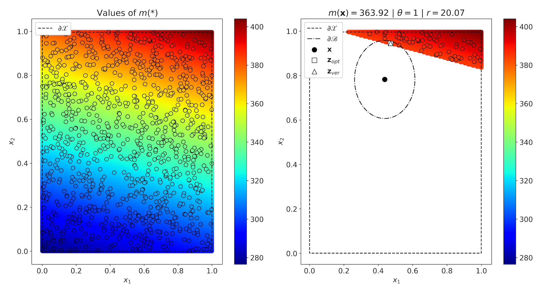
Figure 1: Original and counterfactual points by $\theta=1$ for the black-box Cox model trained on synthetic data

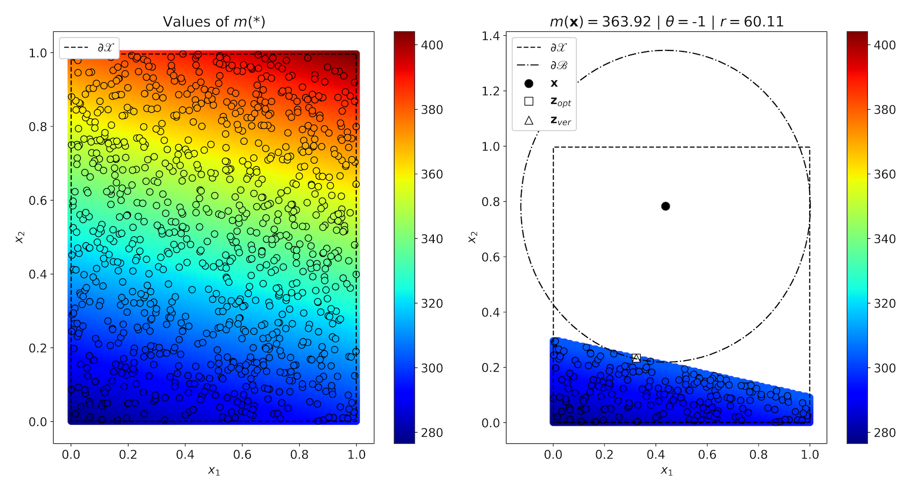
Figure 2: Original and counterfactual points by $\theta=-1$ for the black-box Cox model trained on synthetic data

Similar results cannot be shown for the second type of synthetic data when feature vectors have the dimensionality $20$. Therefore, we give them in Table 1 jointly with numerical results for the two-dimensional data. Parameters $r_{ver}$ and $r_{opt}$ in Table 1 are defined as

$$r_{ver}=\theta\left(m(\mathbf{z}_{ver})-m(\mathbf{x})\right),$$ (45)

$$r_{opt}=\theta\left(m(\mathbf{z}_{opt})-m(\mathbf{x})\right),$$ (46)

respectively. They show the relationship between original margin $r$ and margins $r_{ver}$ and $r_{opt}$ obtained by means of the proposed methods. In fact, values of $r_{ver}$ and $r_{opt}$ indicate how the obtained counterfactuals fulfil condition (11) or condition (12), i.e., conditions

$$\psi(\mathbf{z}_{ver})=r-r_{ver}\leq 0,\ \psi(\mathbf{z}_{opt})=r-r_{opt}\leq 0.$$ (47)

The last three columns also display the relationship between $\mathbf{z}_{ver}$, $\mathbf{z}_{opt}$ and $\mathbf{x}$. In particular, the value of $\left\|\mathbf{z}_{ver}-\mathbf{z}_{opt}\right\|_{2}$ can be regarded as the accuracy measure of the obtained counterfactual.

Table 1: Results of numerical experiments for the black-box Cox model trained on synthetic data

$d$	$\theta$	$r$	$r_{ver}$	$r_{opt}$	$\left\|\mathbf{z}_{ver}-\mathbf{x}\right\|_{2}$	$\left\|\mathbf{z}_{opt}-\mathbf{x}\right\|_{2}$	$\left\|\mathbf{z}_{ver}-\mathbf{z}_{opt}\right\|_{2}$
	$1$	$42.80$	$42.80$	$42.80$	$0.367$	$0.367$	$4.76\times 10^{-6}$
$2$	$-1$	$40.50$	$40.50$	$40.50$	$0.395$	$0.395$	$1.01\times 10^{-6}$
	$1$	$20.07$	$20.07$	$20.07$	$0.166$	$0.166$	$3.72\times 10^{-7}$
	$-1$	$60.11$	$60.11$	$60.11$	$0.561$	$0.561$	$9.93\times 10^{-8}$
	$1$	$238.94$	$238.94$	$238.94$	$0.322$	$0.322$	$1.39\times 10^{-2}$
$20$	$-1$	$206.29$	$206.29$	$206.29$	$0.476$	$0.476$	$1.34\times 10^{-2}$
	$1$	$315.33$	$315.33$	$315.33$	$0.461$	$0.461$	$7.86\times 10^{-3}$
	$-1$	$91.86$	$91.86$	$91.86$	$0.204$	$0.205$	$1.99\times 10^{-2}$

8.1.3 The black-box RSF

The second part of numerical experiments is performed with the RSF as a black-box model. The RSF consists of $250$ decision survival trees. The results are shown in Figs. 3-4. In this cases, $\mathbf{z}_{ver}$ is computed by generating many points ($10^{6}$) and computing $m(\mathbf{z})$ for each point. The counterfactual $\mathbf{z}_{ver}$ minimizes the distance $\left\|\mathbf{z}_{ver}-\mathbf{x}\right\|$ under condition $\psi(\mathbf{z}_{ver})\leq 0$. It can be seen from the pictures that $\mathbf{z}_{ver}$ is again very close to $\mathbf{z}_{opt}$.

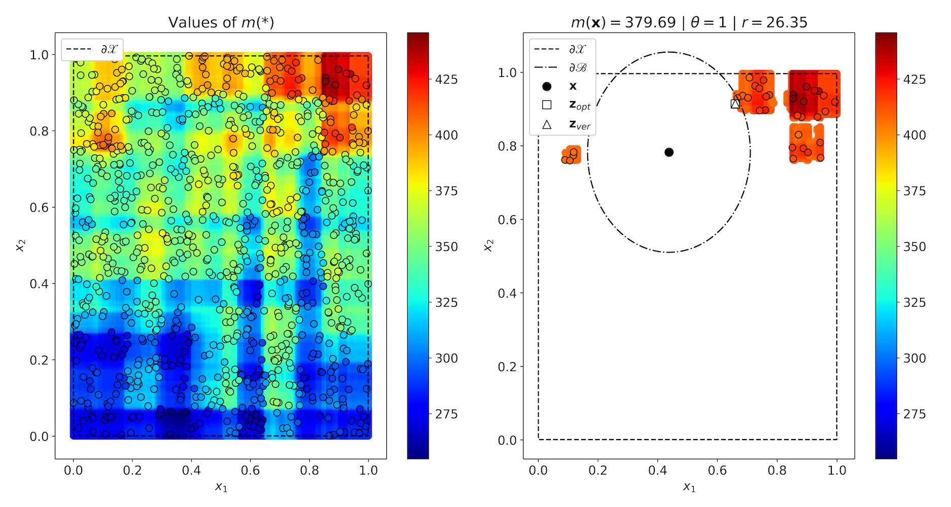
Figure 3: Original and counterfactual points by $\theta=1$ for the black-box RSF trained on synthetic data

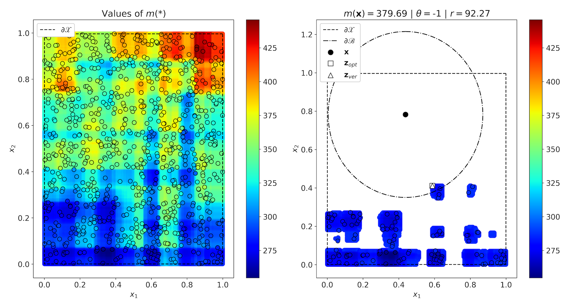
Figure 4: Original and counterfactual points by $\theta=-1$ for the black-box RSF trained on synthetic data

Results of experiments with training data having two- and twenty-dimensional feature vectors are given Table 2. It can be seen from Table 2 that $\mathbf{z}_{opt}$ is not worse ($d=2$) or even better ($d=20$) than $\mathbf{z}_{ver}$ obtained by means of generating the large number of random points (see velues of $A$).

Table 2: Results of numerical experiments for the black-box RSF trained on synthetic data

$d$	$\theta$	$r$	$r_{ver}$	$r_{opt}$	$\left\|\mathbf{z}_{ver}-\mathbf{x}\right\|_{2}$	$\left\|\mathbf{z}_{opt}-\mathbf{x}\right\|_{2}$	$A$
	$1$	$74.81$	$75.67$	$75.39$	$0.153$	$0.153$	$0.0007$
$2$	$-1$	$46.91$	$49.32$	$47.59$	$0.346$	$0.346$	$0.0003$
	$1$	$26.35$	$27.93$	$26.79$	$0.259$	$0.258$	$0.0008$
	$-1$	$92.27$	$92.31$	$92.30$	$0.401$	$0.401$	$0.0006$
	$1$	$229.55$	$232.39$	$229.72$	$0.969$	$0.763$	$0.2062$
$20$	$-1$	$133.46$	$135.84$	$133.50$	$0.876$	$0.563$	$0.3136$
	$1$	$249.88$	$265.91$	$250.15$	$0.982$	$0.641$	$0.3414$
	$-1$	$63.30$	$63.56$	$63.40$	$0.570$	$0.220$	$0.3495$

8.2 Numerical experiments with real data

We consider the following real datasets to study the proposed approach: Stanford2 and Myeloid. The datasets can be downloaded via R package “survival”.

The dataset Stanford2 consists of survival data of patients on the waiting list for the Stanford heart transplant program. It contains 184 patients. The number of features is 2 plus 3 variables: time to death, the event indicator, the subject identifier.

The dataset Myeloid is based on a trial in acute myeloid leukemia. It contains 646 patients. The number of features is 5 plus 3 variables: time to death, the event indicator, the subject identifier. In this dataset, we do not consider the feature “sex” because it cannot be changed. Moreover, we consider two cases for the feature “trt” (treatment arm), when it takes values “A” and “B”. In other words, we divide all patients into two groups depending on the treatment arm. As a result, we have three datasets: Stanford2 and Myeloid-A and Myeloid-B.

8.2.1 The black-box Cox model

Since examples from the dataset Stanford2 have two features which can be changed (age $x_{1}$ and T5 mismatch score $x_{2}$), then results of numerical experiments for this dataset can be visualized, and they shown in Figs. 5-6. We again see that points $\mathbf{z}_{ver}$ and $\mathbf{z}_{opt}$ are close to each other. The same follows from Table 3 which is similar to Table 1, but contains results obtained for real data. If to consider values in the last column of Table 3 as the method accuracy values, then one can conclude that the method provides outperforming results. This means that the Cox model used as a black-box model accurately supports the dataset, and the PSO provides a good solution.

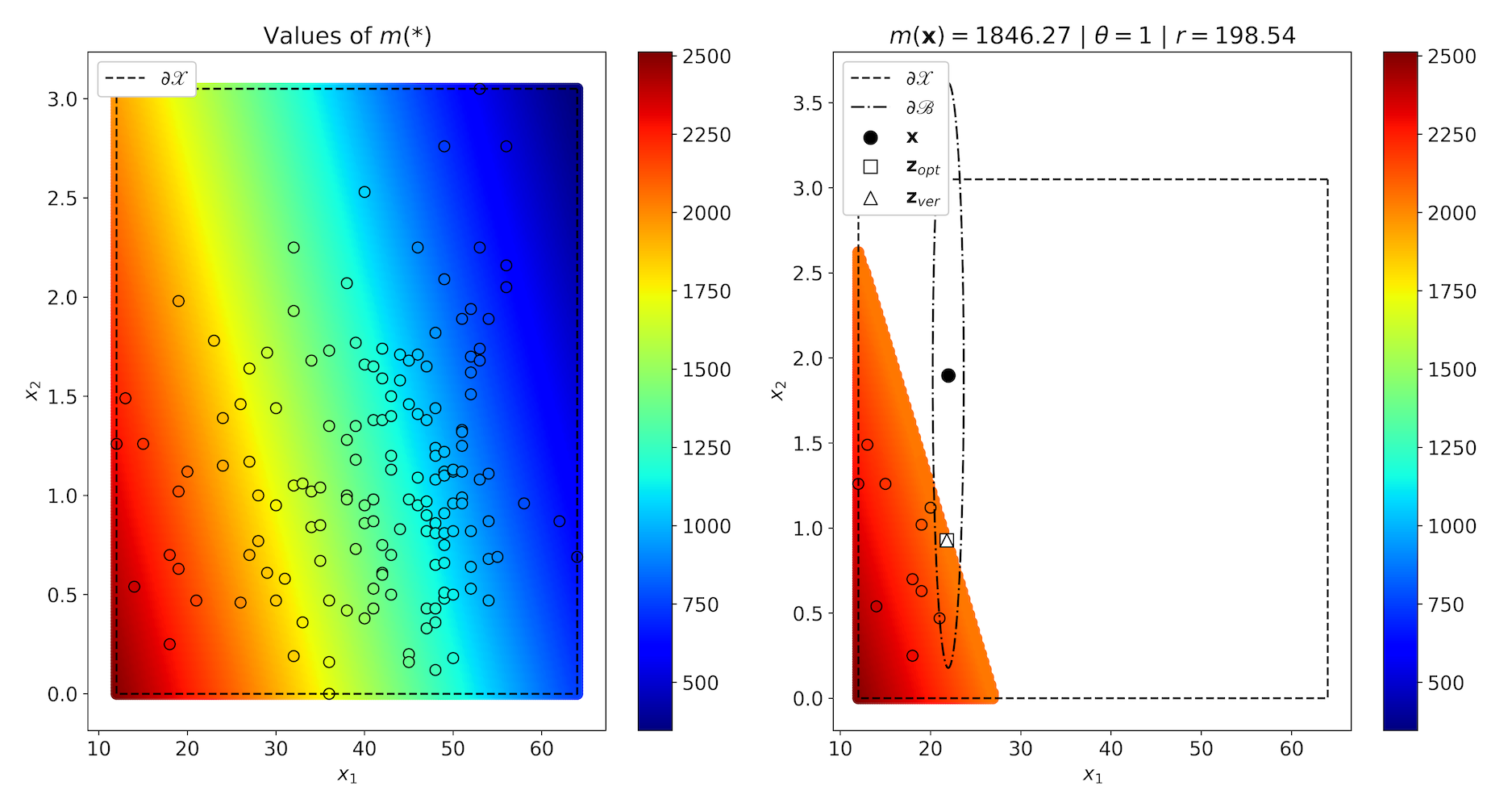
Figure 5: Original and counterfactual points by $\theta=1$ for the black-box Cox model trained on the dataset Stanford2

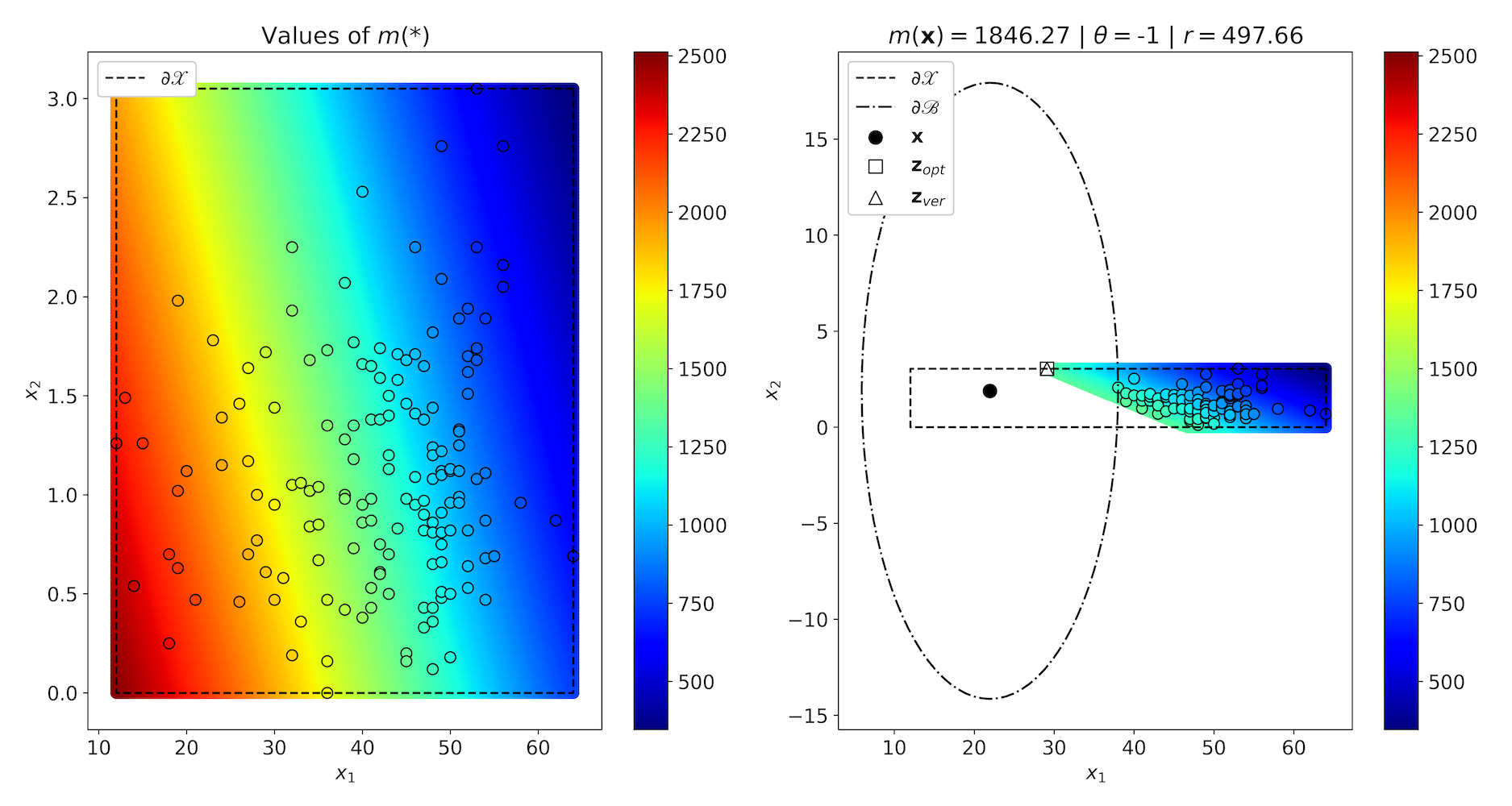
Figure 6: Original and counterfactual points by $\theta=-1$ for the black-box Cox model trained on the dataset Stanford2

Results of experiments with the Cox model trained on datasets Stanford2, Myeloid-A and Myeloid-B are shown in Table 3. One can see that the proposed method also provides exact results for datasets Myeloid-A and Myeloid-B.

Table 3: Results of numerical experiments for the black-box Cox model trained on real data

Dataset	$\theta$	$r$	$r_{ver}$	$r_{opt}$	$\left\|\mathbf{z}_{ver}-\mathbf{x}\right\|_{2}$	$\left\|\mathbf{z}_{opt}-\mathbf{x}\right\|_{2}$	$\left\|\mathbf{z}_{ver}-\mathbf{z}_{opt}\right\|_{2}$
	$1$	$198.54$	$198.54$	$198.54$	$0.983$	$0.983$	$5.62\times 10^{-7}$
Stanford2	$-1$	$497.66$	$497.66$	$497.66$	$7.217$	$7.217$	$7.96\times 10^{-9}$
	$1$	$805.36$	$805.36$	$805.36$	$9.145$	$9.145$	$1.03\times 10^{-8}$
	$-1$	$186.49$	$186.49$	$186.49$	$1.663$	$1.663$	$1.16\times 10^{-8}$
	$1$	$600.05$	$600.05$	$600.05$	$205.937$	$205.937$	$2.36\times 10^{-4}$
Myeloid-A	$-1$	$144.24$	$144.24$	$144.24$	$40.383$	$40.383$	$2.15\times 10^{-5}$
	$1$	$362.00$	$362.00$	$362.00$	$103.535$	$103.535$	$2.16\times 10^{-4}$
	$-1$	$318.66$	$318.66$	$318.66$	$124.692$	$124.692$	$1.11\times 10^{-3}$
	$1$	$57.08$	$57.08$	$57.08$	$28.437$	$28.437$	$2.30\times 10^{-5}$
Myeloid-B	$-1$	$421.76$	$421.76$	$421.76$	$126.749$	$126.749$	$5.10\times 10^{-4}$
	$1$	$206.76$	$206.76$	$206.76$	$260.912$	$260.912$	$2.77\times 10^{-3}$
	$-1$	$498.91$	$498.91$	$498.91$	$124.941$	$124.941$	$4.85\times 10^{-4}$

8.2.2 The black-box RSF

Results for the black-box RSF trained on the dataset Stanford2 are given in Figs. 7-8. We again see that $\mathbf{z}_{ver}$ is close to $\mathbf{z}_{opt}$. Results of experiments with datasets Stanford2, Myeloid-A and Myeloid-B are shown in Table 4. We again see that values of $A\mathbf{\ }$positive for all datasets. This means that the PSO gives better results than the method based on generating the large number of random points.

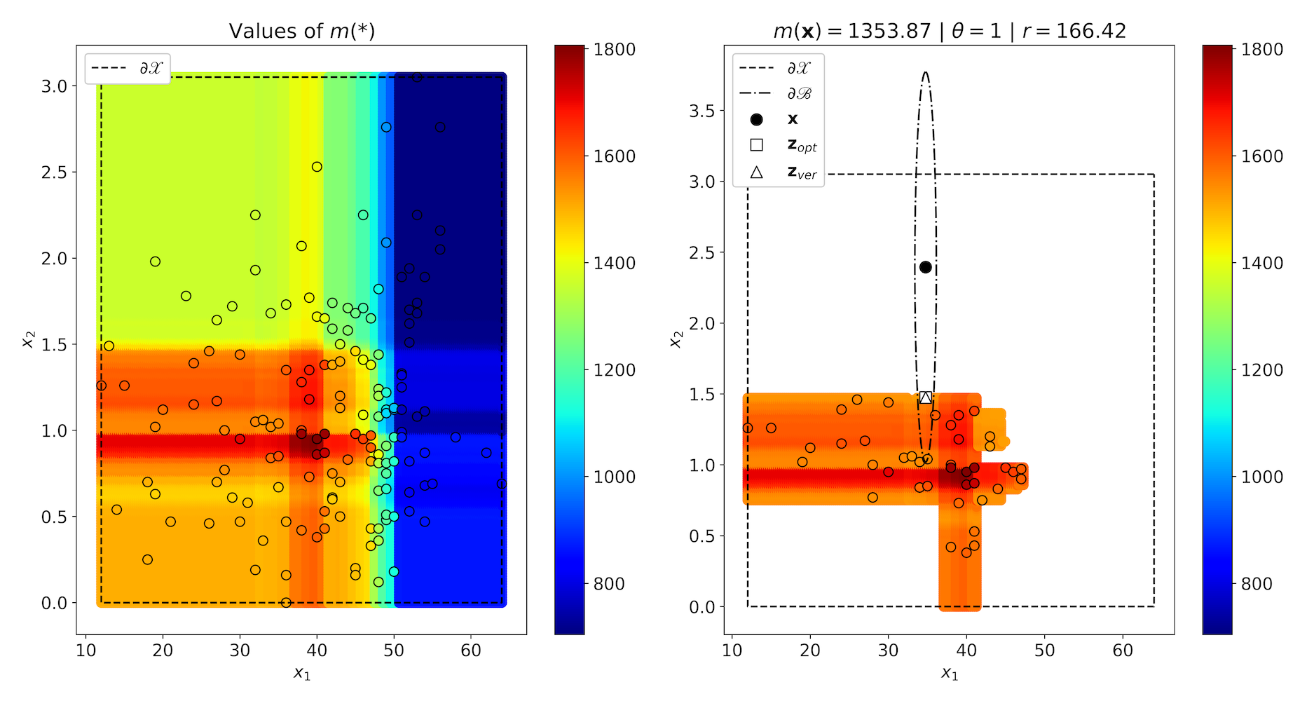
Figure 7: Original and counterfactual points by $\theta=1$ for the black-box RSF trained on the dataset Stanford2

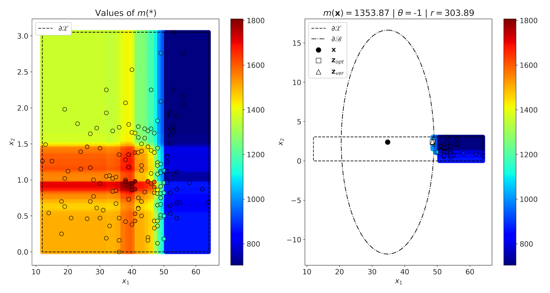
Figure 8: Original and counterfactual points by $\theta=-1$ for the black-box RSF trained on the dataset Stanford2

Table 4: Results of numerical experiments for the black-box RSF trained on real data

Dataset	$\theta$	$r$	$r_{ver}$	$r_{opt}$	$\left\|\mathbf{z}_{ver}-\mathbf{x}\right\|_{2}$	$\left\|\mathbf{z}_{opt}-\mathbf{x}\right\|_{2}$	$A$
	$1$	$225.27$	$236.72$	$236.72$	$0.533$	$0.532$	$0.0006$
Stanford2	$-1$	$417.90$	$418.24$	$418.24$	$27.544$	$27.541$	$0.0027$
	$1$	$166.42$	$171.66$	$171.66$	$0.921$	$0.920$	$0.0002$
	$-1$	$303.89$	$348.91$	$348.91$	$13.738$	$13.738$	$0.0002$
	$1$	$9.26$	$10.10$	$10.10$	$99.917$	$99.689$	$0.2282$
Myeloid-A	$-1$	$36.72$	$37.36$	$37.36$	$275.622$	$274.969$	$0.6532$
	$1$	$6.73$	$10.10$	$10.10$	$130.504$	$130.315$	$0.1888$
	$-1$	$24.66$	$25.03$	$25.03$	$88.392$	$86.078$	$2.3143$
	$1$	$28.52$	$30.02$	$30.02$	$100.882$	$99.770$	$1.1120$
Myeloid-B	$-1$	$197.97$	$200.77$	$198.88$	$523.077$	$521.193$	$1.8838$
	$1$	$2.10$	$5.54$	$5.54$	$123.137$	$122.755$	$0.3818$
	$-1$	$185.27$	$196.00$	$192.56$	$245.575$	$244.157$	$1.4174$

9 Conclusion

One of the important difficulties of using the proposed method is to take into account categorical feature. The difficulty is that the optimization problem cannot handle categorical data and becomes a mixed integer convex optimization problem whose solving is a difficult task in general. Sharma et al. [58] proposed a genetic algorithm called CERTIFAI to partially cope with the problem and for computing counterfactuals. The same problem was studied by Russel [56]. Nevertheless, an efficient solver for this problem is a direction for further research. The same problem takes place in using the PSO. There are some modifications of the original PSO taking into account the categorical and integer features [11, 39, 59]. However, their application to the considered explanation problem is another direction for further research.

We have studied only one criterion for comparison of the SFs of the original example and the counterfactual. This criterion is the difference of mean values. In fact, this criterion implicitly defines different classes of examples. However, other criteria can be applied to the problem and to separating the classes, for example, difference between values of SFs at time moment. The study of other criteria is also an important direction for further research.

Another interesting problem is when the feature vector is a picture, for example, a computer tomography image of an organ. In this case, we have a high-dimensional explanation problem whose efficient solution is also a direction for further research.

References

- [1] A. Adadi and M. Berrada. Peeking inside the black-box: A survey on explainable artificial intelligence (XAI). IEEE Access, 6:52138–52160, 2018.
- [2] I. Ahern, A. Noack, L. Guzman-Nateras, D. Dou, B. Li, and J. Huan. NormLime: A new feature importance metric for explaining deep neural networks. arXiv:1909.04200, Sep 2019.
- [3] A.B. Arrieta, N. Diaz-Rodriguez, J. Del Ser, A. Bennetot, S. Tabik, A. Barbado, S. Garcia, S. Gil-Lopez, D. Molina, R. Benjamins, R. Chatila, and F. Herrera. Explainable artificial intelligence (XAI): Concepts, taxonomies, opportunities and challenges toward responsible AI. arXiv:1910.10045, October 2019.
- [4] V. Arya, R.K.E. Bellamy, P.-Y. Chen, A. Dhurandhar, M. Hind, S.C. Hoffman, S. Houde, Q.V. Liao, R. Luss, A. Mojsilovic, S. Mourad, P. Pedemonte, R. Raghavendra, J. Richards, P. Sattigeri, K. Shanmugam, M. Singh, K.R. Varshney, D. Wei, and Y. Zhang. One explanation does not fit all: A toolkit and taxonomy of AI explainability techniques. arXiv:1909.03012, Sep 2019.
- [5] Q. Bai. Analysis of particle swarm optimization algorithm. Computer and Information Science, 3(1):180–184, 2010.
- [6] S. Barocas, A.D. Selbst, and M. Raghavan. The hidden assumptions behind counterfactual explanations and principal reasons. In Proceedings of the 2020 Conference on Fairness, Accountability, and Transparency, pages 80–89, Barcelona, Spain, 2020. ACM.
- [7] R. Bender, T. Augustin, and M. Blettner. Generating survival times to simulate cox proportional hazards models. Statistics in Medicine, 24(11):1713–1723, 2005.
- [8] L. Breiman. Random forests. Machine learning, 45(1):5–32, 2001.
- [9] V. Buhrmester, D. Munch, and M. Arens. Analysis of explainers of black box deep neural networks for computer vision: A survey. arXiv:1911.12116v1, November 2019.
- [10] D.V. Carvalho, E.M. Pereira, and J.S. Cardoso. Machine learning interpretability: A survey on methods and metrics. Electronics, 8(832):1–34, 2019.
- [11] S. Chowdhury, W. Tong, A. Messac, and J. Zhang. A mixed-discrete particle swarm optimization algorithmwith explicit diversity-preservation. Structural and Multidisciplinary Optimization, 47:367–388, 2013.
- [12] M. Clerc and J. Kennedy. The particle swarm – explosion, stability, and convergence in a multidimensional complex space. IEEE Transactions on Evolutionary Computation, 6(1):58–73, 2002.
- [13] D.R. Cox. Regression models and life-tables. Journal of the Royal Statistical Society, Series B (Methodological), 34(2):187–220, 1972.
- [14] S. Dandl, C. Molnar, M. Binder, and B. Bischl. Multi-objective counterfactual explanations. arXiv:2004.11165, April 2020.
- [15] A. Dhurandhar, P.-Y. Chen, R. Luss, C.-C. Tu, P. Ting, K. Shanmugam, and P. Das. Explanations based on the missing: Towards contrastive explanations with pertinent negatives. arXiv:1802.07623v2, Oct 2018.
- [16] A. Dhurandhar, T. Pedapati, A. Balakrishnan, P.-Y. Chen, K. Shanmugam, and R. Puri. Model agnostic contrastive explanations for structured data. arXiv:1906.00117, May 2019.
- [17] M. Du, N. Liu, and X. Hu. Techniques for interpretable machine learning. arXiv:1808.00033, May 2019.
- [18] D. Faraggi and R. Simon. A neural network model for survival data. Statistics in medicine, 14(1):73–82, 1995.
- [19] C. Fernandez, F. Provost, and X. Han. Explaining data-driven decisions made by AI systems: The counterfactual approach. arXiv:2001.07417, January 2020.
- [20] R. Fong and A. Vedaldi. Explanations for attributing deep neural network predictions. In Explainable AI, volume 11700 of LNCS, pages 149–167. Springer, Cham, 2019.
- [21] R.C. Fong and A. Vedaldi. Interpretable explanations of black boxes by meaningful perturbation. In Proceedings of the IEEE International Conference on Computer Vision, pages 3429–3437. IEEE, 2017.
- [22] D. Garreau and U. von Luxburg. Explaining the explainer: A first theoretical analysis of LIME. arXiv:2001.03447, January 2020.
- [23] Y. Goyal, Z. Wu, J. Ernst, D. Batra, D. Parikh, and S. Lee. Counterfactual visual explanations. arXiv:1904.07451, Apr 2019.
- [24] R. Guidotti, A. Monreale, F. Giannotti, D. Pedreschi, S. Ruggieri, and F. Turini. Factual and counterfactual explanations for black-box decision making. IEEE Intelligent Systems, 34(6):14–23, 2019.
- [25] R. Guidotti, A. Monreale, S. Ruggieri, F. Turini, F. Giannotti, and D. Pedreschi. A survey of methods for explaining black box models. ACM computing surveys, 51(5):93, 2019.
- [26] C. Haarburger, P. Weitz, O. Rippel, and D. Merhof. Image-based survival analysis for lung cancer patients using CNNs. arXiv:1808.09679v1, Aug 2018.
- [27] L.A. Hendricks, R. Hu, T. Darrell, and Z. Akata. Generating counterfactual explanations with natural language. arXiv:1806.09809, June 2018.
- [28] L.A. Hendricks, R. Hu, T. Darrell, and Z. Akata. Grounding visual explanations. In Proceedings of the European Conference on Computer Vision (ECCV), pages 264–279, 2018.
- [29] A. Holzinger, G. Langs, H. Denk, K. Zatloukal, and H. Muller. Causability and explainability of artificial intelligence in medicine. WIREs Data Mining and Knowledge Discovery, 9(4):e1312, 2019.
- [30] D. Hosmer, S. Lemeshow, and S. May. Applied Survival Analysis: Regression Modeling of Time to Event Data. John Wiley & Sons, New Jersey, 2008.
- [31] Q. Huang, M. Yamada, Y. Tian, D. Singh, D. Yin, and Y. Chang. GraphLIME: Local interpretable model explanations for graph neural networks. arXiv:2001.06216, January 2020.
- [32] N.A. Ibrahim, A. Kudus, I. Daud, and M.R. Abu Bakar. Decision tree for competing risks survival probability in breast cancer study. International Journal Of Biological and Medical Research, 3(1):25–29, 2008.
- [33] J.L. Katzman, U. Shaham, A. Cloninger, J. Bates, T. Jiang, and Y. Kluger. Deepsurv: Personalized treatment recommender system using a Cox proportional hazards deep neural network. BMC medical research methodology, 18(24):1–12, 2018.
- [34] J. Kennedy and R.C. Eberhart. Particle swarm optimization. In Proceedings of the International Conference on Neural Networks, volume 4, pages 1942–1948. IEEE, 1995.
- [35] F.M. Khan and V.B. Zubek. Support vector regression for censored data (SVRc): a novel tool for survival analysis. In 2008 Eighth IEEE International Conference on Data Mining, pages 863–868. IEEE, 2008.
- [36] J. Kim, I. Sohn, S.-H. Jung, S. Kim, and C. Park. Analysis of survival data with group lasso. Communications in Statistics - Simulation and Computation, 41(9):1593–1605, 2012.
- [37] M.S. Kovalev and L.V. Utkin. A robust algorithm for explaining unreliable machine learning survival models using the Kolmogorov-Smirnov bounds. arXiv:2005.02249, May 2020.
- [38] M.S. Kovalev, L.V. Utkin, and E.M. Kasimov. SurvLIME: A method for explaining machine learning survival models. Knowledge-Based Systems, 203:106164, 2020.
- [39] E.C. Laskari, K.E. Parsopoulos, and M.N. Vrahatis. Particle swarm optimization for integer programming. In Proceedings of the 2002 Congress on Evolutionary Computation, volume 2, pages 1582–1587. IEEE, 2002.
- [40] T. Laugel, M.-J. Lesot, C. Marsala, X. Renard, and M. Detyniecki. Comparison-based inverse classification for interpretability in machine learning. In Information Processing and Management of Uncertainty in Knowledge-Based Systems. Theory and Foundations. Proceedings of the 17th International Conference, IPMU 2018, volume 1, pages 100–111, Cadiz, Spain, June 2018.
- [41] C. Lee, W.R. Zame, J. Yoon, and M. van der Schaar. Deephit: A deep learning approach to survival analysis with competing risks. In 32nd Association for the Advancement of Artificial Intelligence ( AAAI) Conference, pages 1–8, 2018.
- [42] A. Van Looveren and J. Klaise. Interpretable counterfactual explanations guided by prototypes. arXiv:1907.02584, Jul 2019.
- [43] A. Lucic, H. Oosterhuis, H. Haned, and M. de Rijke. Actionable interpretability through optimizable counterfactual explanations for tree ensembles. arXiv:1911.12199, November 2019.
- [44] S.M. Lundberg and S.-I. Lee. A unified approach to interpreting model predictions. In Advances in Neural Information Processing Systems, pages 4765–4774, 2017.
- [45] U.B. Mogensen, H. Ishwaran, and T.A. Gerds. Evaluating random forests for survival analysis using prediction error curves. Journal of Statistical Software, 50(11):1–23, 2012.
- [46] C. Molnar. Interpretable Machine Learning: A Guide for Making Black Box Models Explainable. Published online, https://christophm.github.io/interpretable-ml-book/, 2019.
- [47] W.J. Murdoch, C. Singh, K. Kumbier, R. Abbasi-Asl, and B. Yua. Interpretable machine learning: definitions, methods, and applications. arXiv:1901.04592, Jan 2019.
- [48] V. Petsiuk, A. Das, and K. Saenko. Rise: Randomized input sampling for explanation of black-box models. arXiv:1806.07421, June 2018.
- [49] R. Poyiadzi, K. Sokol, R. Santos-Rodriguez, T. De Bie, and P. Flach. FACE: Feasible and actionable counterfactual explanations. arXiv:1909.09369, September 2019.
- [50] J. Rabold, H. Deininger, M. Siebers, and U. Schmid. Enriching visual with verbal explanations for relational concepts: Combining LIME with Aleph. arXiv:1910.01837v1, October 2019.
- [51] Y. Ramon, D. Martens, F. Provost, and T. Evgeniou. Counterfactual explanation algorithms for behavioral and textual data. arXiv:1912.01819, December 2019.
- [52] R. Ranganath, A. Perotte, N. Elhadad, and D. Blei. Deep survival analysis. arXiv:1608.02158, September 2016.
- [53] M.T. Ribeiro, S. Singh, and C. Guestrin. “Why should I trust You?” Explaining the predictions of any classifier. arXiv:1602.04938v3, Aug 2016.
- [54] M.T. Ribeiro, S. Singh, and C. Guestrin. Anchors: High-precision model-agnostic explanations. In AAAI Conference on Artificial Intelligence, pages 1527–1535, 2018.
- [55] C. Rudin. Stop explaining black box machine learning models for high stakes decisions and use interpretable models instead. Nature Machine Intelligence, 1:206–215, 2019.
- [56] C. Russel. Efficient search for diverse coherent explanations. arXiv:1901.04909, January 2019.
- [57] S.M. Shankaranarayana and D. Runje. ALIME: Autoencoder based approach for local interpretability. arXiv:1909.02437, Sep 2019.
- [58] S. Sharma, J. Henderson, and J. Ghosh. CERTIFAI: Counterfactual explanations for robustness, transparency, interpretability, and fairness of artificial intelligence models. arXiv:1905.07857, May 2019.
- [59] S. Strasser, R. Goodman, J. Sheppard, and S. Butcher. A new discrete particle swarm optimization algorithm. In Proceedings of the Genetic and Evolutionary Computation Conference, pages 53–60. ACM, 2016.
- [60] E. Strumbel and I. Kononenko. An efficient explanation of individual classifications using game theory. Journal of Machine Learning Research, 11:1–18, 2010.
- [61] R. Tibshirani. The lasso method for variable selection in the cox model. Statistics in medicine, 16(4):385–395, 1997.
- [62] L.V. Utkin, M.S. Kovalev, and E.M. Kasimov. SurvLIME-Inf: A simplified modification of survLIME for explanation of machine learning survival models. arXiv:2005.02387, May 2020.
- [63] J. van der Waa, M. Robeer, J. van Diggelen, M. Brinkhuis, and M. Neerincx. Contrastive explanations with local foil trees. arXiv:1806.07470, June 2018.
- [64] T. Vermeire and D. Martens. Explainable image classification with evidence counterfactual. arXiv:2004.07511, April 2020.
- [65] M.N. Vu, T.D. Nguyen, N. Phan, and M.T. Thai R. Gera. Evaluating explainers via perturbation. arXiv:1906.02032v1, Jun 2019.
- [66] S. Wachter, B. Mittelstadt, and C. Russell. Counterfactual explanations without opening the black box: Automated decisions and the GPDR. Harvard Journal of Law & Technology, 31:841–887, 2017.
- [67] D. Wang, D. Tan, and L. Liu. Particle swarm optimization algorithm: an overview. Soft Computing, 22:387–408, 2018.
- [68] H. Wang and L. Zhou. Random survival forest with space extensions for censored data. Artificial intelligence in medicine, 79:52–61, 2017.
- [69] P. Wang, Y. Li, and C.K. Reddy. Machine learning for survival analysis: A survey. ACM Computing Surveys (CSUR), 51(6):1–36, 2019.
- [70] S. Wang, Y. Zhang, S. Wang, and G. Ji. A comprehensive survey on particle swarm optimization algorithm and its applications. Mathematical Problems in Engineering, 2015(Article ID 931256):1–38, 2015.
- [71] A. White and A.dA. Garcez. Measurable counterfactual local explanations for any classifier. arXiv:1908.03020v2, November 2019.
- [72] A. Widodo and B.-S. Yang. Machine health prognostics using survival probability and support vector machine. Expert Systems with Applications, 38(7):8430–8437, 2011.
- [73] D.M. Witten and R. Tibshirani. Survival analysis with high-dimensional covariates. Statistical Methods in Medical Research, 19(1):29–51, 2010.
- [74] M.N. Wright, T. Dankowski, and A. Ziegler. Unbiased split variable selection for random survival forests using maximally selected rank statistics. Statistics in Medicine, 36(8):1272–1284, 2017.
- [75] N. Xie, G. Ras, M. van Gerven, and D. Doran. Explainable deep learning: A field guide for the uninitiated. arXiv:2004.14545, April 2020.
- [76] H.H. Zhang and W. Lu. Adaptive Lasso for Cox’s proportional hazards model. Biometrika, 94(3):691–703, 2007.
- [77] L. Zhao and D. Feng. Dnnsurv: Deep neural networks for survival analysis using pseudo values. arXiv:1908.02337v2, March 2020.
- [78] X. Zhu, J. Yao, and J. Huang. Deep convolutional neural network for survival analysis with pathological images. In 2016 IEEE International Conference on Bioinformatics and Biomedicine (BIBM), pages 544–547. IEEE, 2016.