Exact Solution of Schrodinger Equation in (Anti-)deSitter Spaces for Hydrogen Atom

Abstract

We write Schrödinger equation for the Coulomb potential in both deSitter and Anti-deSitter spaces using the Extended Uncertainty Principle formulation. We use the Nikiforov-Uvarov method to solve the equations. The energy eigenvalues for both systems are given in their exact forms and the corresponding radial wave functions are expressed in associated Jacobi polynomials for deSitter space, while those of Anti-deSitter space are given in terms of Romanovski polynomials. We have also studied the effect of the spatial deformation parameter on the bound states in the two cases.

PACS: 03.65.Ge, 03.65.Pm.

1 Introduction

The extension of the quantum field theory to curved space-time, which can be considered as a first approximation of quantum gravity has attracted considerable interest as there are strong motivations for absorption of infinities lying in standard field theories. In such situation of curved space-time, we deal with a structure perturbed by the gravitational field. Such modifications can also be found in Snyder model where the measurements in noncommutative quantum mechanics can be governed by a Generalized Uncertainty Principle (GUP) [1]. This model admits a fundamental length scale supposed to be of the order of the Planck length and this is equivalent to a nonzero minimal uncertainty in the measurement of the position [2][3]. Because there are many arguments showing that quantum gravity implies also a minimal measurable length in the order of the Planck length, a large amount of efforts have been devoted to extend the study of the quantum mechanics to a curved space–time via the Extended Uncertainty Principle (EUP) [5]. A significant consequence deduced from this extension is that the minimal length uncertainty in quantum gravity can be related also to a modification of the standard Heisenberg algebra by adding small corrections to the canonical commutation relations [4][6][7]. This was motivated by Doubly Special Relativity (DSR) [8], string theory [9], non-commutative geometry [10] and also black hole physics [11].

In the context of deformed quantum theory with EUP, there are only a few available exact solutions. At the level of relativistic quantum mechanics the list of the exactly solved problems is very restricted, e.g. the case of one-dimensional Dirac and Klein-Gordon oscillators on anti-deSitter (AdS) space was recently considered in [23], the three and two-dimensional Dirac oscillator in the presence of minimal uncertainty in momentum was studied in [24] and the exact solution of (1+1)-dimensional bosonic oscillator subject to the influence of an uniform electric field in AdS space too [25]. On the other hand, the non-relativistic case is also of great interest and remains unexplored within this framework. Despite the fact that, in conventional field theory approach in static de Sitter and anti de Sitter space-time models, we cannot derive any nonrelativistic covariant Schrödinger-like equation from covariant Klein-Fock-Gordon equation, we can use the EUP formulation to write the dS and AdS versions of the Schrödinger equation. Indeed Hamil et al treat the exact solution of the D-dimensional Schrödinger equation for the free-particle and the harmonic-oscillator in AdS space [26]. In [5], Chung study analytically the one dimensional box problem and the harmonic oscillator problem. Also in [6], Ghosh and Mignemi use perturbative methods to study both harmonic oscillator and Hydrogen atom.

Regarding the hydrogen atom and because of the physics that comes from studying and understanding such system, there has been a growing interest in the study of exact solutions of this kind of problem in the ordinary case [12][13][14][15][16] as well as in the context of deformed quantum mechanics based on GUP and we cite here the study of Schrödinger equation for the Coulomb potential with minimal length in one dimension [17][18][19] and in three dimensions [20][22][21].

In this paper, we are looking for the analytical treatment of the hydrogen atom when subject to gravitational effects governed by EUP because it has been studied only perturbatively [6]. For this purpose we solve the non-relativistic Coulomb problem to get the exact form of the energy eigenvalues and eigenfunctions. The paper is organized as follows: In Sec. II 2, we give a review dS and AdS models while In Sec. III LABEL:N-U, we introduce Nikiforov-Uvarov (NU) method that we use to solve equation of our system. We expose in Sec. IV 4, the explicit computations for the hydrogen atom of the deformed Schrödinger equation with EUP and in both dS and AdS cases of the algebra. The energy eigenvalues are given in their exact form and the corresponding radial wave functions are expressed in associated Jacobi polynomials for dS space 4.1 and in terms of Romanovski polynomials for the AdS space 4.2. In the end of this section, we investigate numerically the spectroscopic implications of the EUP deformation. Finally, the concluding remarks come in Sec. V 5.

2 Review on the Deformed Quantum Mechanics Relation

In three-dimensional space, the deformed Heisenberg algebra leading to EUP is defined by the following commutation relations [27][28]

$$\left[X_{i},X_{j}\right]=0\text{ , }\left[P_{i},P_{j}\right]=i\hbar\tau\lambda\epsilon_{ijk}L_{k}\text{ , }\left[X_{i},P_{j}\right]=i\hbar\left(\delta_{ij}-\tau\lambda X_{i}X_{j}\right)\text{ with }\tau=-1,+1$$ (1)

where $\lambda$ is the parameter of the deformation and it is very small because, in the context of quantum gravity, this EUP parameter is determined as a fundamental constant associated to the scale factor of the expanding universe and it is proportional to the cosmological constant $\Gamma=3\tau\lambda=3\tau/a^{2}$ where $a$ is the deSitter radius [29]. $L_{k}$ is the component of the angular momentum expressed by:

$$L_{k}=\epsilon_{ijk}X_{i}P_{j}$$ (2)

and satisfying the usual algebra:

$$\left[L_{i},P_{j}\right]=i\hbar\varepsilon_{ijk}P_{k}\text{ , }\left[L_{i},X_{j}\right]=i\hbar\varepsilon_{ijk}X_{k}\text{ , }\left[L_{i},L_{j}\right]=i\hbar\varepsilon_{ijk}L_{k}$$ (3)

As in ordinary quantum mechanics, the commutation relation 1 gives rise to a Heisenberg uncertainty relation:

$$\Delta X_{i}\Delta P_{i}\geq\frac{\hbar}{2}\left(1-\tau\lambda\left(\Delta X_{i}\right)^{2}\right)$$ (4)

where we choose the states for which $\left\langle X_{i}\right\rangle=0$.

According to the value of $\tau$ we distinguish two kinds of subalgebra. For $\tau=-1$, the deformed algebra is characterized by the presence of a nonzero minimum uncertainty in momentum and it is called Anti-deSitter model. For simplicity, we assume isotropic uncertainties $X_{i}=X$ and this allows us to write the minimal uncertainty for the momentum in AdS model:

$$\left(\Delta P_{i}\right)_{\min}=\hbar\sqrt{\tau\lambda}$$ (5)

For de Sitter model where $\tau=+1$, the relation 4 does not imply an non-zero minimal value for momentum uncertainties.

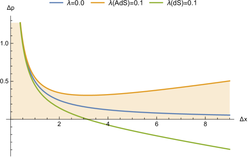
Figure 1: Graphic of HUP and EUP in both dS and AdS Cases

This is shown in figure1 1, where the uncertainty relations are plotted according to the modified relation found in 4. The colored region in 1 is the forbidden area for position and momentum measurements in AdS space.

The noncommutative operators $X_{i}$ and $P_{i}$ satisfy the modified algebra 1 which gives rise to rescaled uncertainty relation 4 in momentum space. In order to study the exact solutions of the deformed Schrödinger equation, we represent these operators as functions of the operators $x_{i}$and $p_{i}$ that satisfy the ordinary canonical commutation relations; This is done thanks to the following transformations:

$$X_{i} =\frac{x_{i}}{\sqrt{1+\tau\lambda r^{2}}}$$ (6a)

$$P_{i} =-i\hbar\sqrt{1+\tau\lambda r^{2}}\partial_{x_{i}}$$ (6b)

If $$\tau=-1 r \left]-1/\sqrt{\lambda},1/\sqrt{\lambda}\right[$$, the variable varies in the domain .

3 Nikiforov–Uvarov Method

The Nikiforov-Uvarov (NU) method was developed basically on the hypergeometric differential equation. The formulas used in NU method reduce the second order differential equations to the hypergeometric type with an appropriate coordinate transformation $s=s\left(x\right)$:

$$\psi^{\backprime\backprime}\left(s\right)+\frac{\tilde{\tau}\left(s\right)}{\sigma\left(s\right)}\psi^{\backprime}\left(s\right)+\frac{\tilde{\sigma}\left(s\right)}{\sigma^{2}\left(s\right)}\psi\left(s\right)=0$$ (7)

where $\sigma\left(s\right)$ and $\widetilde{\sigma}\left(s\right)$ are polynomials of the second degree at most and the degree of the polynomial $\widetilde{\tau}\left(s\right)$ is strictly less than 2 [30][31]. If we take the following factorization:

$$\psi\left(s\right)=\phi\left(s\right)y\left(s\right)$$ (8)

7 becomes [31]:

$$\sigma\left(s\right)y^{\backprime\backprime}\left(s\right)+\tau\left(s\right)y^{\backprime}\left(s\right)+\Lambda y\left(s\right)=0$$ (9)

where:

$$\pi\left(s\right)=\sigma\left(s\right)\frac{d}{ds}\left(\ln\phi\left(s\right)\right)\text{ \ and \ }\tau\left(s\right)=\tilde{\tau}\left(s\right)+2\pi\left(s\right)$$ (10)

$\Lambda$ is defined as:

$$\Lambda_{n}+n\tau^{\backprime}+\frac{n\left(n-1\right)\sigma^{\backprime\backprime}}{2}=0,\text{ \ \ }n=0,1,2,...$$ (11)

And the energy eigenvalues are calculated from the above equation. We first have to determine $\pi\left(s\right)$ and $\Lambda$ by defining:

$$k=\Lambda-\pi^{\backprime}\left(s\right)$$ (12)

Solving the quadratic equation for $\pi\left(s\right)$ with 12, we get

$$\pi\left(s\right)=\left(\frac{\sigma^{\backprime}-\widetilde{\tau}}{2}\right)\pm\sqrt{\left(\frac{\sigma^{\backprime}-\tilde{\tau}}{2}\right)^{2}-\tilde{\sigma}+\sigma k}$$ (13)

Here, $\pi\left(s\right)$ is a polynomial of the parameter $s$ and the prime denotes the first derivative.

One has to note that the determination of $k$ is the essential point in the calculation of $\pi\left(s\right)$ and It is simply defined by stating that the expression under the square root in 13 must be a square of a polynomial; This gives us a general quadratic equation for $k$.

To determine the polynomial solutions $y_{n}\left(s\right)$, we use 10 and the Rodrigues relation:

$$y_{n}\left(s\right)=\frac{C_{n}}{\rho\left(s\right)}\frac{d^{n}}{ds^{n}}\left[\sigma^{n}\left(s\right)\rho\left(s\right)\right]$$ (14)

where $C_{n}$ is normalizable constant and the weight function $\rho\left(s\right)$ satisfies the following relation:

$$\frac{d}{ds}\left[\sigma\left(s\right)\rho\left(s\right)\right]=\tau\left(s\right)\rho\left(s\right)$$ (15)

This last equation refers to the classical orthogonal polynomials that have many important properties and especially orthogonality defined by:

$$\int_{a}^{b}y_{n}\left(s\right)y_{m}\left(s\right)\rho\left(s\right)ds=0\text{ if }m\neq n$$ (16)

4 Schrödinger Equation for the Hydrogen Atom in (Anti-)deSitter Space

In this section, we study the effects of deformed space on the energy eigenvalues and eigenfunctions of a hydrogen atom in the context of the non-relativistic quantum mechanics. In the case of a three-dimensional space,we consider the following stationary Schrödinger equation with a Coulomb-type interaction:

$$\left[\frac{\mathbf{p}^{2}}{2m}-\frac{e^{2}}{r}\right]\psi\left(\mathbf{r}\right)=E\psi\left(\mathbf{r}\right)\,$$ (17)

In order to include the effect of EUP on the above Schrödinger equation, we use the transformations LABEL:eqt16a and 6b to obtain:

$$\left[-\frac{\hbar^{2}}{2m}\left[\left(1+\tau\lambda r^{2}\right)\left(\frac{\partial^{2}}{\partial r^{2}}+\frac{2}{r}\frac{\partial}{\partial r}-\frac{L^{2}}{\hbar^{2}r^{2}}\right)+\tau\lambda r\frac{\partial}{\partial r}\right]-\frac{e^{2}\sqrt{1+\tau\lambda r^{2}}}{r}\right]\psi=E\psi$$ (18)

 

In order to separate the variables, we write the solution as $\psi(r,\theta)=r^{-1/2}R(r)Y_{l}^{m_{l}}(\theta,\varphi)$ and this enables us to split the equation into two parts, one angular and the other radial (where $\chi\equiv\sqrt{1+\tau\lambda r^{2}}$):

$$L^{2}Y_{l}^{m_{l}}(\theta,\varphi)=\hbar^{2}l\left(l+1\right)Y_{l}^{m_{l}}(\theta,\varphi)\,$$ (19)

$$\left[\left(\chi\frac{d}{dr}\right)^{2}+\frac{\chi^{2}}{r}\frac{d}{dr}-\frac{\left(l\left(l+1\right)+\frac{1}{4}\right)\chi^{2}}{r^{2}}+\frac{2me^{2}\chi}{\hbar^{2}r}\right]R(r)=-\left(\frac{2mE}{\hbar^{2}}+\frac{\tau\lambda}{2}\right)R(r)$$ (20)

The angular equation of the system is just the usual one for spherical harmonics, so we are interested in the resolution of the radial one. In order to do this, we use the following transformations:

$$s=\frac{\sqrt{1+\tau\lambda r^{2}}}{\sqrt{\lambda}r}$$ (21)

Then, the new form of 20 becomes:

$$\left[\left(1-\tau s^{2}\right)^{2}\frac{d^{2}}{ds^{2}}-\tau s\left(1-\tau s^{2}\right)\frac{d}{ds}-\left(l+\frac{1}{2}\right)^{2}s^{2}+\eta s+\varepsilon\right]R_{1,2}(s)=0\,$$ (22)

where

$$\eta=\frac{2me^{2}}{\hbar^{2}\sqrt{\lambda}}\text{ and\ }\varepsilon=\frac{2mE}{\lambda\hbar^{2}}+\frac{\tau}{2}$$ (23)

4.1 Solutions for deSitter Space ($\tau=+1$)

Comparison between 22 and 7 allows us to use the NU method where the expressions of the polynomials appearing in 7 are given by:

$$\sigma\left(s\right)=\left(1-s^{2}\right)\text{ , }\tilde{\tau}\left(s\right)=-s\text{ \ and }\tilde{\sigma}\left(s\right)=-\left(l+\frac{1}{2}\right)^{2}s^{2}+\eta s+\varepsilon$$ (24)

Substituting them into 13 we obtain:

$$\pi\left(s\right)=\frac{-s}{2}\pm\sqrt{\left(\frac{1}{4}+\left(l+\frac{1}{2}\right)^{2}-k\right)s^{2}-\eta s+k-\varepsilon}$$ (25)

Where the parameter $k$ is to be determined by the condition mentioned in the section III LABEL:N-U. One then obtains the following possible solutions for each $k$:

$$\pi\left(s\right)=\left\{\begin{array}[c]{c}\pi_{1,2}=\left(\frac{-1}{2}\pm\delta_{1}\right)s\mp\frac{\eta}{2\delta_{1}}\text{\ for\ }k_{1}=\frac{1}{2}\left[\varepsilon+\frac{1}{4}+\left(l+\frac{1}{2}\right)^{2}+\sqrt{\Delta}\right]\\ \pi_{3,4}=\left(\frac{-1}{2}\pm\delta_{2}\right)s\mp\frac{\eta}{2\delta_{2}}\text{\ for\ }k_{2}=\frac{1}{2}\left[\varepsilon+\frac{1}{4}+\left(l+\frac{1}{2}\right)^{2}-\sqrt{\Delta}\right]\end{array}\right.$$ (26)

with:

$$\delta_{1,2}=\sqrt{\frac{1}{4}+\left(l+\frac{1}{2}\right)^{2}-k_{1,2}}\text{ and }\Delta=\left(\varepsilon-\frac{1}{4}-\left(l+\frac{1}{2}\right)^{2}\right)^{2}-\eta^{2}$$ (27)

Here, we choose the proper value $\pi_{1}$, so that:

$$\tau\left(s\right)=2\left(\delta_{1}-1\right)s-\frac{\eta}{\delta_{1}}$$ (28)

From 11 we obtain:

$$\Lambda=k_{1}-\frac{1}{2}+\delta_{1}=n_{r}\left(n_{r}+1-2\delta_{1}\right)\text{ , }n_{r}=0,1,2,...$$ (29)

Hence, the energy eigenvalues are found as:

$$E_{n,l}=-\frac{me^{4}}{2\hbar^{2}n^{2}}-\frac{\lambda\hbar^{2}}{2m}\left(n^{2}-l\left(l+1\right)-1\right)$$ (30)

where $n=n_{r}+l+1$ is the principal quantum number.

We remark that the above expression of energies contains the usual Hydrogen term and an additional correction term proportional to the deformation parameter $\lambda$, so we recover the Bohr energies when the deformation disappears. It should be noted here that the first term of the correction is proportional to $n{{}^{2}}$ and so it is equivalent to the energy of a non-relativistic quantum particle moving in a square well potential; In our case, the boundaries of the well are placed at $\pm\pi/2\sqrt{\lambda}$. The second term in the correction contains the azimuthal quantum number $l$ and it removes the $\left(2l+1\right)$ degeneracy of the energy levels. We also notice that the correction deformation affects all energy levels except the ground level ($n=1$) which remains not affected by the deformation even for large values of $\lambda$.

Now let us find the corresponding eigenfunctions. Taking the expression of $\pi_{1}\left(s\right)$ from 26, the $\phi\left(s\right)$ part is defined from the relation 10 as below:

$$\phi\left(s\right)=\left(1+s\right)^{\frac{1}{4}\left(1-2\delta_{1}-\frac{\eta}{\delta_{1}}\right)}\left(1-s\right)^{\frac{1}{4}\left(1-2\delta_{1}+\frac{\eta}{\delta_{1}}\right)}$$ (31)

and according to the form of $\sigma\left(s\right)$ 24, the $y\left(s\right)$ part is given by Rodrigues relation:

$$y_{n}\left(s\right)=\frac{C_{n}}{\rho\left(s\right)}\frac{d^{n}}{ds^{n}}\left[\left(1-s^{2}\right)^{n}\rho\left(s\right)\right]$$ (32)

where $\rho\left(s\right)=\left(1+s\right)^{\left(-\delta_{1}-\frac{\eta}{2\delta_{1}}\right)}\left(1-s\right)^{-\left(\delta_{1}-\frac{\eta}{2\delta_{1}}\right)}$. The expression 32 stands for the Jacobi polynomials as:

$$y_{n}\left(s\right)\equiv P_{n_{r}}^{\left(-\delta_{1}-\frac{\eta}{2\delta_{1}},-\delta_{1}+\frac{\eta}{2\delta_{1}}\right)}\left(s\right)$$ (33)

Hence, $R_{dS}(s)$ can be written in the following form:

$$R_{dS}(s)=C_{n}\left(1-s\right)^{\frac{1}{4}\left(1-2\delta_{1}+\frac{\eta}{\delta_{1}}\right)}\left(1+s\right)^{\frac{1}{4}\left(1-2\delta_{1}-\frac{\eta}{\delta_{1}}\right)}P_{n_{r}}^{\left(-\delta_{1}-\frac{\eta}{2\delta_{1}},-\delta+\frac{\eta}{2\delta_{1}}\right)}\left(s\right)$$ (34)

In terms of the variables $r$, $\theta$ and $\varphi$, we can now write the general form of the wave function $\Psi$ as follows:

$$\Psi_{n_{r}}\left(r,\theta,\varphi\right) =C_{n}\left(1-\frac{\sqrt{1+\lambda r^{2}}}{\sqrt{\lambda}r}\right)^{\frac{1}{4}\left(1-2\delta_{1}+\frac{\eta}{\delta_{1}}\right)}\left(1+\frac{\sqrt{1+\lambda r^{2}}}{\sqrt{\lambda}r}\right)^{\frac{1}{4}\left(1-2\delta_{1}-\frac{\eta}{\delta_{1}}\right)}\times$$

$$P_{n_{r}}^{\left(-\delta_{1}-\frac{\eta}{2\delta_{1}},-\delta_{1}+\frac{\eta}{2\delta_{1}}\right)}\left(\frac{\sqrt{1+\lambda r^{2}}}{\sqrt{\lambda}r}\right)Y_{l}^{m_{l}}(\theta,\varphi)\,$$ (35)

where $C_{n}$ is a normalization constant.

4.2 Solutions for Anti-deSitter Space ($\tau=-1$)

By comparing 22 with 7, we determine NU polynomials as follows:

$$\sigma\left(s\right)=\left(1+s^{2}\right)\text{ ,\ }\tilde{\tau}\left(s\right)=s\text{ and }\tilde{\sigma}\left(s\right)=-\left(l+\frac{1}{2}\right)^{2}s^{2}+\eta s+\varepsilon$$ (36)

Substituting them into 10, we obtain:

$$\pi\left(s\right)=\frac{s}{2}\pm\sqrt{\left(k+\frac{1}{4}+\left(l+\frac{1}{2}\right)^{2}\right)s^{2}-\eta s+k-\varepsilon}$$ (37)

The constant $k$ is determined in the same way as in dS case. Therefore, we get:

$$\pi\left(s\right)=\left\{\begin{array}[c]{c}\pi_{1,2}=\left(\frac{1}{2}\pm\delta_{1}^{\backprime}\right)s\mp\frac{\eta}{2\delta_{1}^{\backprime}}\text{\ for\ }k_{1}^{\backprime}=\frac{1}{2}\left[\varepsilon-\frac{1}{4}-\left(l+\frac{1}{2}\right)^{2}-\sqrt{\vartriangle^{\backprime}}\right]\\ \pi_{3,4}=\left(\frac{1}{2}\pm\delta_{2}^{\backprime}\right)s\mp\frac{\eta}{2\delta_{2}^{\backprime}}\text{\ for\ }k_{2}^{\backprime}=\frac{1}{2}\left[\varepsilon-\frac{1}{4}-\left(l+\frac{1}{2}\right)^{2}+\sqrt{\vartriangle^{\backprime}}\right]\end{array}\right.$$ (38)

where:

$$\delta_{1,2}^{\backprime}=\sqrt{\frac{1}{4}+\left(l+\frac{1}{2}\right)^{2}+k_{1,2}^{\backprime}}\text{ and }\Delta^{\backprime}=\left(\varepsilon+\frac{1}{4}+\left(l+\frac{1}{2}\right)^{2}\right)^{2}+\eta^{2}$$ (39)

Here, we choose the proper value $\pi_{2}$, so that we have:

$$\tau\left(s\right)=2\left(1-\delta_{1}^{\backprime}\right)s-\frac{\eta}{\delta_{1}^{\backprime}}$$ (40)

From 11, we calculate:

$$\Lambda=k_{1}^{\backprime}+\frac{1}{2}-\sqrt{\frac{1}{4}+\left(l+\frac{1}{2}\right)^{2}+k_{1}^{\backprime}}=-n_{r}\left(n_{r}+1-2\sqrt{\frac{1}{4}+\left(l+\frac{1}{2}\right)^{2}+k_{1}^{\backprime}}\right)$$ (41)

Hence, the energy eigenvalues are found as:

$$E_{n,l}=-\frac{me^{4}}{2\hbar^{2}n^{2}}+\frac{\lambda\hbar^{2}}{2m}\left(n^{2}-l\left(l+1\right)-1\right)$$ (42)

The same remarks made in the case of dS space apply here except that in this case the correcting terms are inversely proportional to the deformation parameter $\lambda$, so that the energies increases with increasing values of $\lambda$ and the bound states in AdS space become less bounded than those of the dS case for the same value of $\lambda$ 3042.

In both cases, the spectral corrections due to EUP are qualitatively different to those associated to GUP [20].

Now, to deduce the complete expression of the wave functions $\Psi_{n}\left(x\right)$, we use the expression 38 of $\pi_{2}\left(s\right)$ as follows:

$$\phi\left(s\right)=\left(1+s^{2}\right)^{\frac{1}{2}\left(\frac{1}{2}-\delta_{1}^{\backprime}\right)}e^{\frac{-\eta}{2\delta_{1}^{\backprime}}\tan^{-1}\left(s\right)}$$ (43)

and using Rodrigues formula 14, we find

$$y_{n}\left(s\right)=\frac{C_{n}^{\backprime}}{\rho\left(s\right)}\frac{d^{n}}{ds^{n}}\left[\left(1+s^{2}\right)^{n}\rho\left(s\right)\right]$$ (44)

where $\rho\left(s\right)=\left(1+s^{2}\right)^{-\delta_{1}^{\backprime}}e^{\frac{\eta}{\delta_{1}^{\backprime}}\tan^{-1}\left(s\right)}$.

The relation 44 stands for the Romanovski polynomials [32] as:

$$y_{n}\left(s\right)\equiv R_{n}^{\left(-\delta_{1}^{\backprime},\frac{-\eta}{\delta_{1}^{\backprime}}\right)}\left(s\right)=\frac{C_{n}^{\backprime}}{\left(1+s^{2}\right)^{-\delta_{1}^{\backprime}}e^{\frac{-\eta}{\delta_{1}^{\backprime}}\tan^{-1}\left(s\right)}}\frac{d^{n}}{ds^{n}}\left[\left(1+s^{2}\right)^{n-\delta_{1}^{\backprime}}e^{\frac{-\eta}{\delta_{1}^{\backprime}}\tan^{-1}\left(s\right)}\right]$$ (45)

Consequently, the expression of $R_{AdS}(s)$ is written as:

$$R_{AdS}(s)=C_{n}\left(1+s^{2}\right)^{\frac{1}{2}\left(\frac{1}{2}-\delta_{1}\right)}e^{\frac{-\eta}{2\delta_{1}}\tan^{-1}\left(s\right)}R_{n}^{\left(-\delta_{1},\frac{-\eta}{\delta_{1}}\right)}\left(s\right)$$ (46)

and the expression of the wave function $\Psi$ with the former variables $r$, $\theta$ and $\varphi$ is given by:

$$\Psi_{n}\left(r,\theta,\varphi\right)=C_{n}^{\backprime}\left(\sqrt{\lambda}r\right)^{\left(\delta_{1}^{\backprime}-\frac{1}{2}\right)}e^{\frac{-\eta}{2\delta_{1}^{\backprime}}\tan^{-1}\left(\frac{\sqrt{1-\lambda r^{2}}}{\sqrt{\lambda}r}\right)}R_{n}^{\left(-\delta_{1}^{\backprime},\frac{-\eta}{\delta_{1}^{\backprime}}\right)}\left(\frac{\sqrt{1-\lambda r^{2}}}{\sqrt{\lambda}r}\right)Y_{l}^{m_{l}}(\theta,\varphi)\,$$ (47)

with $C_{n}^{\backprime}$ is a normalization constant.

In order to show the effects of the deformed Heisenberg algebra leading to EUP on the bound-states of the Coulomb potential in non-relativistic quantum mechanics systems, we plot, as an example, the energies levels of the $s-$states $E_{n,0}$ versus the deformation parameters $\lambda$ for different values of $n$ (we use the Hartree atomic units $m=\hbar=e=4\pi\varepsilon_{0}$ $=1$).

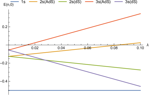
Figure 2: $E_{n,0}(\lambda)$ for $n=1,2$ & $3$ in dS and AdS cases

According to the results shown in figure2 2 and to the expression of the energies 42, it is clear that the deformation increases the energies in AdS case and thus decreases the binding energies of the states. We thus arrive at a critical point where the value of the deformation parameter cancels the bound state or $E_{n,l}=0$:

$$\lambda_{c}(n,l)=\frac{1}{n^{2}\left(n^{2}-l\left(l+1\right)-1\right)}$$ (48)

This critical values of the spatial deformation parameter can be interpreted as a resonance point because the corresponding state of the atomic system ionizes. We give in table1 Table1 some critical values $\lambda_{c}(n,l)$ corresponding to the first levels. Note from 30 that this is not the case for dS space because the deformation increases the bonding of atomic states and so no ionization effect occurs here.

$$\lambda_{c}(n,l)$$

   (Table1)

Figure2 2 and to the expression of the dS energies 30 show that the deformation can reverse the order of energy levels since the correction depends on the main quantum number. If we take the level $n=3$ as an example, we see that it decreases faster than the $2^{nd}$ level and therefore it becomes lower. Then it continues to decrease until it becomes lower than the $1^{st}$ level, which will no longer be the fundamental one. The value of $\lambda$ that causes this inversion between the upper levels and the fundamental one is calculated from 30:

$$\lambda_{f}(n,l)=\frac{n^{2}-1}{n^{2}\left(n^{2}-l\left(l+1\right)-1\right)}$$ (49)

In table2 Table2, we give some numerical values of $\lambda_{f}(n,l)$.

$$\lambda_{f}(n,l)$$

   (Table2)

Using 5, we see that the main feature of the hydrogen spectrum in AdS model 42 is the presence of an additional positive correction proportional to the nonzero minimal uncertainty:

$$E_{n,l}=-\frac{mk^{2}e^{4}}{2\hbar^{2}n^{2}}+\frac{\Delta P_{\min}^{2}}{2m}\left(n^{2}-l\left(l+1\right)-1\right)$$ (50)

One can use this relation to obtain an upper bound on the EUP deformed parameter $\lambda\$from spectroscopic considerations and we choose the $2s-1s$ transition line:

$$\frac{E_{2s}-E_{1s}}{E_{1s}}=-\frac{3}{4}-\frac{3}{2}\frac{\hbar^{2}}{m^{2}k^{2}e^{4}}\Delta P_{\min}^{2}$$ (51)

Taking the experimental results for this transition in the hydrogen atom where the precision is of the order of $\varepsilon\approx 10^{-15}$ [33] and if we attribute this error entirely to the EUP correction 50, we can write:

$$\varepsilon=\frac{3}{2}\frac{\hbar^{2}}{m^{2}k^{2}e^{4}}\Delta P_{\min}^{2}$$ (52)

Therefore, the upper bound of the minimal uncertainty in momentum is given by $\Delta P_{\min}\sim 10^{-32}Jsm^{-1}$; This value is much smaller than the one obtained in [24].

5 Conclusion

In this work, we have analytically studied the deformed Schrödinger equation in three dimensions for a Hydrogen atom in deSitter and Anti-deSitter spaces by using the position representation of the Extended Uncertainty Principle formulation and the Nikiforov–Uvarov method. For both cases, we obtained the exact eigen-energies and eigen-functions. The radial wave functions were expressed as associated Jacobi polynomials for deSitter space and in terms of Romanovski polynomials for Anti-deSitter space.

The deformed energy spectrum was written as the usual Coulomb term with an additional correction term that removes the $l$ degeneracy of Bohr energies. The main effect of the deformation parameter $\lambda$ is an increase of the energies for AdS spaces and a decrease of these energies for dS spaces. It should be noted here that the two spectra are similar to those arising when considering the non-relativistic model for Hydrogen atom in space of constant negative and positive curvature: hyperbolic Lobachevsky and spherical Riemann models [34] (and the references therein).

In the AdS case, we showed that, due to the decrease of the binding energies with increasing $\lambda$ values, we reach a critical point where the corresponding state is no longer bound and thus becomes ionized or diffusive. The critical values $\lambda_{c}(n,l)$ are inversely proportional to the quantum numbers $n$ and $l$; so higher levels ionize one after the other as $\lambda$ increases, until the stage where the atomic system contains only the fundamental level. This is explained by the fact that the higher states are more easily ionized even in the ordinary case.

On the other hand, in the case of dS space, all the energies levels are more bounded proportionally to the values of the EUP parameter. Because bound energies are increased according to $\lambda$ in this case, the deformation can cause a reversal of the order of the levels where the energy of the higher levels are diminished until becoming smaller than that of the fundamental level. The corresponding values to this phenomenon $\lambda_{f}(n,l)$ are also inversely proportional to the quantum numbers $n$ and $l$.

These two effects of ionization and inversion are comparable to an extension of the higher levels in the case AdS and a contraction of these same levels in the case of dS.

Finally, in order to see the effect of the deformation on the physical systems, we compared them with the experimental results of the non-relativistic hydrogen atom and we have determined a satisfactory value of the upper bound of minimal momentum uncertainty for AdS space.

References

- [1] H. S. Snyder, Quantized Space-Time, Phys. Rev. 71, 38-41 (1947)
- [2] A. Kempf, Uncertainty relation in quantum mechanics with quantum group symmetry, J. Math. Phys. 35, 4483-4496 (1994); A. Kempf, G. Mangano, and R. B. Mann, Hilbert space representation of the minimal length uncertainty relation, Phys. Rev. D 52, 1108-1118 (1995)
- [3] R. Vilela Mendes, The Geometry of Noncommutative Space-Time, Int. J. Thoer. Phys. 56, 259-269 (2017)
- [4] S. Mignemi, Extended uncertainty principle and the geometry of (anti)-de Sitter space, Mod. Phys. Lett. A 25, 1697-1703 (2010)
- [5] W. S. Chung; The New Type of Extended Uncertainty Principle and Some Applications in Deformed Quantum Mechanics; Int. J. Theor. Phys 58, 2575–2591 (2019)
- [6] S. Ghosh, S. Mignemi, Quantum Mechanics in de Sitter Space, Int. J. Theor. Phys. 50, 1803-1808 (2011)
- [7] K. Nozari, P. Pedram and M. Molkara, Minimal Length, Maximal Momentum and the Entropic Force Law, Int. J. Theor. Phys. 51, 1268-1275 (2012)
- [8] G. Amelino-Camelia, Testable scenario for Relativity with minimum-length, Phys. Lett. B 510, 255-263 (2001); G. Amelino-Camelia, Relativity in space-times with short-distance structure governed by an observer-independent (Planckian) length scale, Int. J. Mod. Phys. D 11, 35-60 (2002)
- [9] S. Capozziello, G. Lambiase, and G. Scarpetta, Generalized Uncertainty Principle from Quantum Geometry, Int. J. Theor. Phys. 39, 15-22 (2000)
- [10] M. R. Douglas and N. A. Nekrasov, Noncommutative field theory, Rev. Mod. Phys. 73, 977-1029 (2001)
- [11] F. Scardigli, Generalized Uncertainty Principle in Quantum Gravity from Micro-Black Hole Gedanken Experiment, Phys. Lett. B 452, 39-44 (1999); F. Scardigli and R. Casadio, Generalized uncertainty principle, extra dimensions and holography, Class. Quant. Grav. 20, 3915-3926 (2003)
- [12] J. A. Reyes and M. del Castillo-Mussot, 1D Schrödinger equations with Coulomb-type potentials, J. Phys. A: Math. Gen. 32, 2017-2025 (1999)
- [13] Y. Ran, L. Xue, S. Hu and R-K. Su, On the Coulomb-type potential of the one-dimensional Schrödinger equation, J. Phys. A: Math. Gen. 33, 9265-9272 (2000)
- [14] A. N. Gordeyev and S. C. Chhajlany, One-dimensional hydrogen atom: a singular potential in quantum mechanics, J. Phys. A: Math. Gen. 30, 6893-6909 (1997)
- [15] I. Tsutsui, T. Fulop and T. Cheon., Connection conditions and the spectral family under singular potentials, J. Phys. A: Math. Gen. 36, 275-287 (2003)
- [16] H. N. N. Yepez, C. A. Vargas and A. L. S. Brito, The one-dimensional hydrogen atom in momentum representation, Eur. J. Phys. 8 189-193 (1987)
- [17] P. Pedram, A note on the one-dimensional hydrogen atom with minimal length uncertainty, J.Phys.A. 45 505304 (2012)
- [18] K. Nouicer, Coulomb potential in one dimension with minimal length: A path integral approach, J. Math. Phys. 48, 112104 (2007)
- [19] T. V. Fityo, I. O. Vakarchuk, and V. M. Tkachuk, One-dimensional Coulomb-like problem in deformed space with minimal length, J. Phys. A 39, 2143-2149 (2006)
- [20] F. Brau, Minimal length uncertainty relation and the hydrogen atom, J. Phys. A 32, 7691-7696 (1999)
- [21] S. Benczik, L. N. Chang, D. Minic, and T. Takeuchi, Hydrogen-atom spectrum under a minimal-length hypothesis, Phys. Rev. A 72, 012104 (2005)
- [22] R. Akhoury and Y. P. Yao, Minimal Length Uncertainty Relation and the Hydrogen Spectrum, Phys. Lett. B 572, 37-42 (2003)
- [23] B. Hamil and M. Merad, Dirac and Klein-Gordon oscillators on anti-de Sitter space, Eur. Phys. J. Plus 133, 174 (2018)
- [24] B. Hamil and M. Merad, Dirac Equation in the Presence of Minimal Uncertainty in Momentum, Few-Body Syst 60, 36 (2019)
- [25] M. Hadj Moussa and M. Merad, Relativistic Oscillators in Generalized Snyder Model, Few-Body Syst 59, 44 (2018)
- [26] B. Hamil, M. Merad and T. Birkandan, Applications of the extended uncertainty principle in AdS and dS spaces, Eur. Phys. J. Plus 134, 278 (2019)
- [27] S. Mignemi, Classical and quantum mechanics of the nonrelativistic Snyder model in curved space, Class. Quant. Grav. 29, 215019 (2012)
- [28] M. M. Stetsko, Dirac oscillator and nonrelativistic Snyder-de Sitter algebra, J. Math. Phys. 56, 012101 (2015)
- [29] B. Bolen and M. Cavaglià, (Anti-)de Sitter black hole thermodynamics and the generalized uncertainty principle, Gen. Relativ. Gravit. 37, 1255-1262 (2005)
- [30] H. Egrifes, D. Demirhan and F. Buyukkiliç, Exact Solutions of the Schrödinger Equation for Two ”Deformed” Hyperbolic Molecular Potentials, Phys. Scripta 59, 195-198 (1999)
- [31] A. F. Nikiforov and V. B. Uvarov, Special Functions of Mathematical Physics, Birkhauser Basel, (1988)
- [32] A. P. Raposo, H. J. Weber, D. E. Alvarez-Castillo and M. Kirchbach, Romanovski polynomials in selected physics problems, Cent. Eur. J. Phys. 5, 253-284 (2007)
- [33] A. Matveev et al, Precision Measurement of the Hydrogen Frequency via a 920-km Fiber Link, Phys. Rev. Lett. 110, 230801 (2013)
- [34] V.M. Redkov and E.M. Ovsiyuk, Quantum mechanics in spaces of constant curvature, Nova Science Publishers. Inc., New York, (2012)