ML Models of Vibrating H₂CO: Comparing Reproducing Kernels, FCHL and PhysNet

Abstract

Machine Learning (ML) has become a promising tool for improving the quality of atomistic simulations. Using formaldehyde as a benchmark system for intramolecular interactions, a comparative assessment of ML models based on state-of-the-art variants of deep neural networks (NN), reproducing kernel Hilbert space (RKHS+F), and kernel ridge regression (KRR) is presented. Learning curves for energies and atomic forces indicate rapid convergence towards excellent predictions for B3LYP, MP2, and CCSD(T)-F12 reference results for modestly sized (in the hundreds) training sets. Typically, learning curve off-sets decay as one goes from NN (PhysNet) to RKHS+F to KRR (FCHL). Conversely, the predictive power for extrapolation of energies towards new geometries increases in the same order with RKHS+F and FCHL performing almost equally. For harmonic vibrational frequencies, the picture is less clear, with PhysNet and FCHL yielding respectively flat learning at $\sim 1$ and $\sim 0.2$ cm^-1 no matter which reference method, while RKHS+F models level off for B3LYP, and exhibit continued improvements for MP2 and CCSD(T)-F12. Finite-temperature molecular dynamics (MD) simulations with the same initial conditions yield indistinguishable infrared spectra with good performance compared with experiment except for the high-frequency modes involving hydrogen stretch motion which is a known limitation of MD for vibrational spectroscopy. For sufficiently large training set sizes all three models can detect insufficient convergence (“noise”) of the reference electronic structure calculations in that the learning curves level off. Transfer learning (TL) from B3LYP to CCSD(T)-F12 with PhysNet indicates that additional improvements in data efficiency can be achieved.

University of Basel]Department of Chemistry, University of Basel, Klingelbergstrasse 80 , CH-4056 Basel, Switzerland. University of Basel]Department of Chemistry, University of Basel, Klingelbergstrasse 80 , CH-4056 Basel, Switzerland. University of Basel]Department of Chemistry, University of Basel, Klingelbergstrasse 80 , CH-4056 Basel, Switzerland.

1 Introduction

With the advent of machine learning (ML) in the physical sciences a paradigm shift has taken place ^{1, 2, 3, 4}. In particular for molecular sciences where the interaction between particles is of central importance for developing quantitatively meaningful models, ML offers many opportunities for improved and computationally efficient modeling of systems. This also leads to the question which - if any - of the existing and currently pursued approaches to represent inter- and intramolecular potential energy surfaces is most advantageous. Such an assessment includes questions pertaining to how “data hungry” a particular approach is (i.e. how much data is required to achieve a given level of accuracy for a particular property), how accurate the resulting PES is, whether the model can be used to extrapolate to unknown regions not sampled by the reference data and finally, whether computed observables from the models differ or whether they are largely insensitive to the representation and its quality given the same reference data set. All these points will be assessed in the present work for formaldehyde (H₂CO, see Figure 1).

Formaldehyde is a small molecule for which very high-level calculations have already been presented ^{5, 6, 7} and experimental reference data is available to compare with ⁸. Apart from its suitability for in-depth theoretical study, formaldehyde is also interesting because it (i) is an important precursor in chemical industries ⁹ (ii) plays an ubiquitous role in many domains including biology, atmosphere, toxicology, interstellar chemistry ^{10, 11, 12, 13} and (iii) was first implicated in the phenomenon of ’roaming’ ¹⁴.

Earlier theoretical work on formaldehyde includes a global PES based on CCSD(T)/aug-cc-pVTZ and MR-CI/aug-cc-pVTZ calculations for which different fits are smoothly joined using switching functions⁵ and a newer, refined global PES employing multi reference configuration interaction (MRCI/cc-pVTZ) calculations.⁶ The root mean squared error (RMSE) of the fit to the CCSD(T)/aug-cc-pVTZ data ranged from 277 cm^-1 to 648 cm^-1 (0.8 to 1.9 kcal/mol), depending on the energy range considered (10000 to 38500 cm^-1).⁵ For this fit, Morse-type variables had been used. For the more recent global PES,⁶ fit to permutationally invariant polynomials and based on MRCI reference data, the averaged RMS error was 100 cm^-1. Both surfaces were used to study roaming.

The present work compares three currently available ML approaches using the same reference data sets computed at three representative levels of quantum chemical rigor (Hybrid density functional approximation (B3LYP)^{15, 16}, Møller Plesset 2^nd order perturbation theory (MP2)¹⁷, and Coupled Cluster Single Doubles perturbative Triples (CCSD(T)-F12))¹⁸. The three ML methods are also meant to be representative in that they range from a purely kernel-based approach (reproducing kernel Hilbert space - RKHS^{19, 20} plus forces (RKHS+F)²¹) to a purely neural network (NN) based approach (PhysNet ²²), and include the FCHL representation ²³ within kernel ridge regression (KRR). It should be mentioned that there is obviously a considerably larger number of alternative methods, equally suited quantum chemistry and ML methods that could have been used just as well. However, the limited present selection is largely due to the focus on the particular system, formaldehyde, and its particular properties relevant to intramolecular interactions.

The present work is structured as follows. First, the three ML methods are introduced, followed by a description of how the data sets were generated and how vibrational spectra were computed. The results compare the mutual performance of the ML methods by considering energy and force learning curves, harmonic frequencies and IR spectra from finite-temperature MD simulations at the highest level of quantum chemical theory. This is followed by a discussion and conclusion.

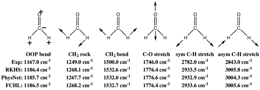
Figure 1: Molecular structure and the directions of the normal modes for formaldehyde (H₂CO). “+” and “-” indicate motions with respect to the plane containing all four atoms. Experimental IR frequencies ($\nu_{4}$, $\nu_{6}$, $\nu_{3}$, $\nu_{2}$, $\nu_{1}$, and $\nu_{5}$) in ascending order of the experiments⁸ are reported together with harmonic frequencies obtained from ML models trained on the largest CCSD(T)-F12 data set size.

2 Theory

In the following the machine learning methods, the generation of the data sets including the structure sampling procedure and the quantum chemical calculations are explained. Then, the computation of vibrational spectra is reviewed.

2.1 Machine Learning Methods

In this section the ML methods used in the present work are introduced and specifics about them are given.

2.1.1 PhysNet

High-dimensional PESs can be constructed using PhysNet which is a NN of the “message-passing” type.²⁴ So-called feature vectors are learned to encode a representation of the local chemical environment of each atom. In an iterative fashion, the initial feature vector depending only on nuclear charges $Z_{i}$ and Cartesian coordinates $\bm{r}_{i}$ of all atoms $i$ is adjusted by passing “messages” between atoms. Based on the learned feature vectors, PhysNet predicts atomic energy contributions and partial charges for arbitrary geometries of the molecule. The total potential energy of the system corresponds to $E=\sum_{i=1}^{N}E_{i}$, where $E_{i}$ are the atomic energy contributions. The partial charges $q_{i}$ are corrected to assure that the total charge of the system is conserved according to the following scheme:

$$\tilde{q}_{i}=q_{i}-\frac{1}{N}\left(\sum_{j=1}^{N}q_{j}-Q\right)$$ (1)

Here, $\tilde{q}_{i}$ are the corrected partial charges, $q_{i}$ are the partial charges predicted by PhysNet and $Q$ is the total charge of the system ²². The forces $\bm{F}_{i}$ required to run MD simulations are calculated analytically by reverse mode automatic differentiation ²⁵.

During training the PhysNet parameters are adjusted to best describe the reference energies, forces and dipole moments from quantum chemical calculations. The optimization uses “adaptive moment estimation” (ADAM) ²⁶. For a detailed description of the PhysNet architecture as well as fitting procedure the reader is referred to Reference 22.

2.1.2 Kernel-based methods

Next, two kernel-based methods to represent potential energy surfaces are detailed. The first method (“RKHS+F”) is based on reproducing kernel Hilbert spaces²⁷ and uses a distance-based representation, while the second method uses a regressor from Gaussian process regression combined with the Faber-Christensen-Huang-Lilienfeld representation (“FCHL”), which is a refined spatial representation based on radial and angular spectra.^{23, 28} Kernel-based methods explore the possibility to formulate the task of fitting a PES as an inversion problem. The theory of these methods asserts that for $N$ given data points $\mathbf{x}_{i}$ of a function $f_{i}=f(\mathbf{x}_{i})$, the value of $f(\mathbf{x})$ at an arbitrary point $\mathbf{x}$ can always be approximated as a linear combination of kernel products²⁹

$$f(\mathbf{x})=\sum_{i=1}^{N}\alpha_{i}K(\mathbf{x},\mathbf{x}_{i})$$ (2)

Here, the $\alpha_{i}$ are regression coefficients and $K(\mathbf{x},\mathbf{x^{\prime}})$ is a kernel function. The coefficients $\alpha_{i}$ can be determined from inverting

$$f_{j}=\sum_{i=1}^{N}\alpha_{i}K_{ij}$$ (3)

using, e.g. Cholesky decomposition³⁰, where $K_{ij}=K(\mathbf{x}_{i},\mathbf{x}_{j})$ is the symmetric, positive-definite kernel matrix. With this, the value of $f(\mathbf{x})$ for an arbitrary argument $\mathbf{x}$ can be calculated using Eq. 2.

Specifics for RKHS+F
For higher-dimensional problems the RKHS+F method used here constructs $D$-dimensional kernels as tensor products of one-dimensional kernels $k(x,x^{\prime})$

$$K(\mathbf{x},\mathbf{x_{i}})=\prod_{d=1}^{D}k^{(d)}(x^{(d)},x_{i}^{(d)})$$ (4)

For the kernel functions $k(x,x^{\prime})$ it is possible to encode physical knowledge, such as their long range interactions which has been done for weakly interacting systems.³¹ The general expression for the 1D kernel function used here is

$$k^{[n,m]}=n^{2}x_{>}^{-(m+1)}B(m+1,n)_{2}F_{1}\left(-n+1,m+1;n+m+1;\frac{x_{<}}{x_{>}}\right)$$ (5)

where, $n$ and $m$ are the smoothness and asymptotic reciprocal power parameters, whereas $x_{<}$ and $x_{>}$ are the smaller and larger value of $x$, respectively. $B(a,b)$ in Eq. 5 is the beta function $B(a,b)=\frac{(a-1)!(b-1)!}{(a+b-1)!}$ and ${}_{2}F_{1}(a,b;c;z)$ is Gauss’ hypergeometric function.¹⁹ For different types of bonds it may be necessary to choose different kernel functions.

Within a many body expansion, the total potential energy of a system can be decomposed into a sum of $p$-body interactions $V^{(p)}$. For a molecule with $n$ atoms, each $p$-body term consists of ${}^{n}C_{p}$ $p$-body interactions, where ${}^{n}C_{p}$ is the binomial coefficient. The total potential for an $n$-atomic species is therefore

$$V=\sum_{p=1}^{n}\sum_{i=1}^{{}^{n}C_{p}}V_{i}^{(p)}$$ (6)

In practice Eq. 6 is truncated at $p=3$ or 4. Here, $p=4$ was used, i.e. all many-body terms were included.

In the present study, each term of the $p$-body interaction energy is represented as an $M$-dimensional ($M=$ ${}^{p}C_{2}$) reproducing kernel constructed from $M$ reciprocal power kernels for $M$ interatomic distances $r_{j}$. The full kernel is then

$$K({\bf r},{\bf r^{\prime}})=\sum_{p=1}^{n}\sum_{l=1}^{{}^{n}C_{p}}\prod_{j=1}^{{}^{p}C_{2}}k_{j}(r_{j},r^{\prime}_{j})$$ (7)

and

$$V({\bf r})=\sum_{i=1}^{N}\alpha_{i}K({\bf r},{\bf r^{\prime}})$$ (8)

Here, ${\bf r}$ is a vector containing all pairwise interatomic distances of an $n$-atomic system, ${\bf r}=\{r_{h}|h=1,2,3\cdots,^{n}C_{2}$}. In the present study, $k^{[3,5]}$, $k^{[3,1]}$ and $k^{[3,0]}$ kernel functions are used to construct mono/multidimensional kernels for 2-, 3-, and 4-body interaction energies, respectively.

The symmetry of a molecule is explicitly included in the total kernel polynomial $K({\bf r},{\bf r^{\prime}})$ (see Eq. 7) by expanding it as a linear combination of all equivalent structures of a molecule. Examples are shown in Ref. 21 for CH₄ and CH₂O.

Specifics for FCHL
An alternative approach to representing the molecules comes from recent developments in machine learning representations for molecules.³² These often allow for improved learning rates at the cost of increased model complexity. The FCHL representation²³ used in this work describes the atomic environment of an atom as histograms based on the radial distribution of surrounding atoms and Fourier terms for the angular distributions. This makes it possible to train models that span molecules and materials of varying sizes and chemical composition. For forces and energies, the “FCHL19” representation is used, which is a coarse-grained, discretized, and numerically efficient implementation of FCHL with pre-optimized hyper-parameters for force and energy learning.²⁸

FCHL relies on the “localized” kernel ansatz, to ensure size-extensivity and permutational atom index invariance.³³ Here, it is used together with a Gaussian kernel function where the kernel element between two molecules corresponds to the sum of pair-wise Gaussian kernel functions between atoms in the respective two molecules:

$$\mathbf{K}_{ij}=\sum_{I\in i}\sum_{J\in i}\delta_{Z_{I}Z_{J}}\exp\left(-\frac{\|\mathbf{x}_{I}-\mathbf{x}_{J}\|^{2}_{2}}{2\sigma^{2}}\right)$$ (9)

where $\mathbf{x}_{I}$ and $\mathbf{x}_{J}$ are the representation of the $I$’th and $J$’th atoms in the molecules $i$ and $j$, respectively, and the Kronecker-$\delta$ between $Z_{I}$ and $Z_{J}$ (their atomic numbers) ensuring bagging, as demonstrated previously to be advantageous for universal quantum ML models based on the bag-of-bonds representation ³⁴.

Regression for RKHS+F: Derivatives of the potential with respect to the distance coordinates can be calculated analytically up to order $(n-1)$ by simply replacing the kernel polynomial $K({\bf r},{\bf r^{\prime}})$ by their derivatives $K^{\prime}({\bf r},{\bf r^{\prime}})$. Using the chain rule, gradients with respect to Cartesian coordinates can also be obtained, which are also available from the electronic structure calculations. For an RKHS+F-based representation of the PES, the set of linear equations can be written as a matrix equation

$$\begin{bmatrix}\mathbf{v}\\ \mathbf{f}\end{bmatrix}=\begin{bmatrix}\mathbf{K}&\\ -\frac{\partial}{\partial\mathbf{r}}\mathbf{K}&\end{bmatrix}\bm{\alpha},$$ (10)

where $\mathbf{v}$ and $\mathbf{f}$ are vectors containing energies and forces, respectively, and $\bm{\alpha}$ is a vector containing a set of regression coefficients. For an $n-$atomic species the matrix in the left hand side becomes rectangular with dimension $(3n+1)N\times N$ Eq. 10 are solved using a least square fitting algorithm. The ‘DGELSS’ subroutine in the LAPACK library is used to solve the set of linear equations.

Regression for FCHL: For the model using the FCHL representation, a model for energies and forces is implemented similarly to what is commonly known from Gaussian process regression and kernel-ridge regression with derivatives.^{35, 36} Here, a PES can be regressed from the training set of molecules with reference energy and force labels. By placing the kernel functions and corresponding kernel derivatives on the molecules in the training set, the set of equations to train or predict energies and forces are^{35, 37}

$$\begin{bmatrix}\mathbf{v}\\ \mathbf{f}\end{bmatrix}=\begin{bmatrix}\mathbf{K}&&-\frac{\partial}{\partial\mathbf{r}^{\top}}\mathbf{K}\\ -\frac{\partial}{\partial\mathbf{r}}\mathbf{K}&&\frac{\partial^{2}}{\partial\mathbf{r}\partial\mathbf{r}^{\top}}\mathbf{K}\end{bmatrix}\bm{\alpha}.$$ (11)

This is akin (except for using the Hessian) to Eq. 10 for the RKHS+F approach, but with an extended set of basis functions. Similarly to both RKHS+F and PhysNet, forces can be evaluated as the derivative of the energy, which is crucial for energy conservation.

The optimal regression coefficients $\bm{\alpha}$ can then be obtained, for example, by minimizing the following cost function:

$$J(\bm{\alpha})=\frac{1}{2}\left\lVert\begin{bmatrix}\mathbf{K}&&-\frac{\partial}{\partial\mathbf{r}^{\top}}\mathbf{K}\\ -\frac{\partial}{\partial\mathbf{r}}\mathbf{K}&&\frac{\partial^{2}}{\partial\mathbf{r}\partial\mathbf{r}^{\top}}\mathbf{K}\end{bmatrix}\bm{\alpha}-\begin{bmatrix}\mathbf{v}^{\mathrm{ref}}\\ \mathbf{f}^{\mathrm{ref}}\end{bmatrix}\right\rVert_{2}^{2}+\frac{\lambda}{2}\bm{\alpha}^{\top}\begin{bmatrix}\mathbf{K}&&-\frac{\partial}{\partial\mathbf{r}^{\top}}\mathbf{K}\\ -\frac{\partial}{\partial\mathbf{r}}\mathbf{K}&&\frac{\partial^{2}}{\partial\mathbf{r}\partial\mathbf{r}^{\top}}\mathbf{K}\end{bmatrix}\bm{\alpha}$$ (12)

where $\lambda$ is a regularizer that puts a small penalty on large regression coefficients and ensures numerical stability to the minimizer. Compared with RKHS+F, FCHL uses second derivatives (see Eq. 11) which increases computational cost but also further improves performance²⁸ (vide infra).

For dipole moments, the analytical implementation of the FCHL L2-norm in Eqn. 9 (i.e. “FCHL18”) is used as previously described.³⁸ The implementation adds a dependence on an externally applied field $\mathbf{E}$ to the representation via a set of fictitious atomic partial charges. For non-zero fields, this component is crucial in order to ensure that the uniqueness condition of a representation can be met ³⁹. The result is a physics based representation for machine learning models of the dipole moment, as obtained by differentiating ML model of the energy with respect to field. More specifically, the following relations of the kernel-based energy model are used:

$$\mathbf{v}=\mathbf{K}\bm{\alpha}$$ (13)

and the relationship between energy and dipole moment

$$\bm{\mu}=-\frac{\partial}{\partial\vec{\mathbf{E}}}\mathbf{v}$$ (14)

leads to

$$\bm{\mu}=\left[-\frac{\partial}{\partial\vec{\mathbf{E}}}\mathbf{K}\right]\bm{\alpha}$$ (15)

The regression coefficients can be obtained by minimizing a cost function such as

$$J(\bm{\alpha})=\tfrac{1}{2}\left\lVert\left[-\tfrac{\partial}{\partial\vec{\mathbf{E}}}\mathbf{K}\right]\bm{\alpha}-\bm{\mu}^{\mathrm{ref}}\right\rVert_{2}^{2}$$ (16)

in a least squares fit. In practice, a singular-value decomposition of the kernel derivative matrix is used via the LAPACK subroutine DGELSD.

For simplicity the Gasteiger-Marsili charge model⁴⁰ as implemented in Open Babel⁴¹ is used to obtain the fictitious charges but the learned model has been found to depend little on the choice of the fictitious charges³⁸, as long as they are physically reasonable, since the numerical values of the partial charges will be absorbed into the regression coefficients.

3 Methods

3.1 Quantum Chemical Calculations

The reference energies, forces and dipole moments are obtained from quantum chemical calculations at different levels of theory and using different quantum chemical programs. They include the B3LYP^{15, 16}/cc-pVDZ⁴² level of theory calculated using Orca⁴³, and the MP2¹⁷/aug-cc-pVTZ⁴⁴ and the CCSD(T)-F12¹⁸/aug-cc-pVTZ-F12⁴⁵ levels of theory obtained from Molpro ⁴⁶ calculations. Loose convergence criteria on the Hartree-Fock reference wave function can lead to noise in the energies and forces used in the training. Therefore, tighter convergence criteria were used as follows. For Orca the SCF convergence criterion (“VeryTightSCF”) and the DFT integration grid (“Grid7” and “NoFinalGrid”) were used. For calculations with Molpro the convergence criteria are tightened using the “gthresh” keyword and set to “gthresh,orbital=1.d-8, gthresh,energy=1.d-11” and “gthresh,orbital=1.d-8, gthresh,energy=1.d-12” for the MP2/aug-cc-pVTZ and the CCSD(T)-F12/aug-cc-pVTZ-F12 calculations, respectively.

3.2 Data Set

To assess the performance of the different approaches, two data sets were generated. Set1 contains $N_{\rm tot}=4001$ H₂CO structures including the optimized H₂CO structure. It was randomly split into subsets (training and test set) of different sizes. The geometries were generated by means of normal mode sampling.⁴⁷ Starting from the optimized H₂CO structure at the B3LYP/cc-pVDZ level of theory and knowing the normal mode coordinates together with their harmonic force constants, distorted conformations were obtained by randomly displacing the atoms along the normal modes. To capture the equilibrium, room temperature and higher energy regions of the PES the normal mode sampling was carried out at eight different temperatures (10 K, 50 K, 100 K, 300 K, 500 K, 1000 K, 1500 K, 2000 K). For each temperature 500 structures were generated.

For assessing the extrapolation capabilities of the different ML methods, a second data set (Set2) was generated which also contains distorted structures, not sampled in Set1. For this, 2500 structures were generated from normal mode sampling carried out at 5000 K.

The ML models are trained on different training set sizes from Set1, including $N_{\rm train}=100$, 200, 400, 800, 1600, and 3200 structures and tested on the remaining $N_{\rm tot}-N_{\rm train}$ structures. Therefore, the indices of the structures are shuffled (based on a seed) and the training set was taken to be $[0:N_{\rm train}]$. For each training set size (and ML method and level of theory) a total of five independent models are trained, where a different seed is used for the shuffling of the indices. To guarantee direct comparability of the different ML methods the models are trained and tested on exactly the same reference data.

3.3 Vibrational Spectra

Vibrational spectra were computed by means of normal mode analysis and finite-temperature molecular dynamics (MD) simulations. These simulations were carried out using the atomic simulation environment (ASE)⁴⁸ together with the best respective ML model trained on the CCSD(T)-F12 data. For direct comparison of the different ML models the MD simulations were started from identical initial conditions, i.e. the same molecular geometry and initial momenta. The initial geometry was the optimized H₂CO structure from the FCHL-based model which is identical to the minimized structures from the other two methods, see Tables S2 to S4 and the momenta were drawn randomly from a Maxwell-Boltzmann distribution and scaled to correspond to exactly 300 K. The optimized geometries from the ab initio calculations as well as optimized using the ML models are listed in Tables S1 to S4.

First, the molecule was equilibrated in the $NVE$ ensemble for 50 ps, followed by MD simulations with a time step of $\Delta t=0.5$ fs for a total of 200 ps. When running the simulation with PhysNet, the molecular dipole moment $\bm{\mu}=\sum_{i=1}^{N}q_{i}\bm{r}_{i}$ is calculated and saved simultaneously for each snapshot of the trajectory, whereas for FCHL computing the dipole moment is a post processing step. With RKHS+F no dipole moment was learned. Instead, PhysNet was used to obtain the molecular dipole for the structures sampled in the simulations with the RKHS+F PES.

The infrared spectra are then obtained from the Fourier transform of the dipole-dipole auto-correlation function $C(t)=\langle\bm{\mu}(0)\bm{\mu}(t)\rangle$. Using the efficient Fast Fourier Transform algorithm from the numpy python library, the transform $C(\omega)$ is obtained using a Blackman filter. In addition, for PhysNet 1000 independent trajectories were run following the same protocol outlined above using the unscaled momenta drawn from a Boltzmann distribution at 300 K. From this, a conformationally averaged IR spectrum was calculated to test convergence.

4 Results

The performance of the models is determined by considering the mean absolute error (MAE) and the RMSE for energy $E$ and forces $F$. This is done for the test set and for the extrapolation data set, the learning curves, for the harmonic frequencies and the (anharmonic) frequencies obtained from finite temperature MD.

4.1 Learning Curves

Learning curves report the out-of-sample prediction error as a function of training set size. They are a useful way to compare different ML techniques on the same footing and to assess how rapidly they reach a particular accuracy.

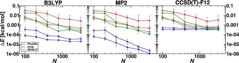
Figure 2: Energy learning curves (Log-log plot) for the PhysNet- (red), FCHL- (blue) and RKHS+F- (green) based models. All models are trained on the same reference data with different data set sizes (100, 200, 400, 800, 1600, 3200) and on data calculated at different levels of theory (B3LYP, MP2, and CCSD(T)-F12 from left to right). The MAE is shown as a circle and the RMSE is shown as a triangle. $\Delta E$ corresponds to the energy error and the error bars indicate the minimum and maximum error. Every data point is an average over 5 models trained independently on the same data set size, but different samples from the full data set.

Figure 2 reports energy learning curves of PhysNet, RKHS+F, and FCHL using the three quantum chemical reference methods B3LYP, MP2, and CCSD(T)-F12. For all reference methods systematic improvement of predictive power is observed as the training set size increases, reaching very good accuracies of at least $10^{-3}$ kcal/mol (compared with $\sim 1$ kcal/mol from earlier work fit to CCSD(T) reference data).⁵ Among the ML methods tested, FCHL yields the lowest errors, followed by RKHS+F and PhysNet. For the two largest training set sizes (1600, 3200), the learning curve of PhysNet ceases to learn, except for B3LYP. This could be due to the fact that PhysNet, as it is common among ANNs, represents a non-parametric supervised ML model. Interestingly, the deviation among MAE and RMSE is larger for PhysNet than for the kernel-based methods. Significant differences among various error measures of prediction error statistics of KRR machine learning models were recently studied in great detail⁴⁹, suggesting that further analysis also including NN-based models is warranted.

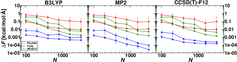
Figure 3: Force learning curves (log-log plot) for the PhysNet- (red), FCHL- (blue) and RKHS+F- (green) based models. All models are trained with different data set sizes (100, 200, 400, 800, 1600, 3200) and on data of different levels of theory. The MAE is shown as a circle and the RMSE is shown as a triangle. $\Delta F$ corresponds to the force error and the error bars indicate the minimum and maximum error. Every data point is an average over 5 models trained independently on the same data set size, but different samples from the full data set.

The impact of reference method selection on learning curves is considerable: For MP2, all ML models exhibit steep learning curves which do not saturate, for the kernel based models in particular and with FCHL reaching a MAE of $10^{-6}$ kcal/mol. By contrast, when using CCSD(T)-F12 as a reference, rapid convergence towards an error floor of several $10^{-4}$ kcal/mol is observed for all ML models. Learning curves for the B3LYP reference lie in between these two extremes, converging for FCHL towards an error floor of several $10^{-5}$ kcal/mol. The existence of such floors in learning curves of functional machine learning models suggests that there is “noise” in the data. Indeed, inspection of the literature indicates that the forces in MOLPRO at the CCSD(T)-F12 level are less accurate than machine-precision.⁵⁰ Before using the data set in the current learning study, the existence of such noise-levels was not known to the authors. The learning curve of FCHL obtained for B3LYP references may display a similar effect, e.g. resulting from noise due to unconverged integration settings. Additional testing supports this explanation: Using B3LYP calculations with standard convergence criteria for SCF iterations and integration grid, the learning curve floors are confirmed for all three ML models. It is, therefore, concluded that ML is capable of detecting such subtle convergence issues in unseen data sets. The force learning curves, see Figure 3, and learning curves for the dipole moment (for PhysNet- and FCHL-based models, see Figure S4) display a similar pattern as the energy learning curves.

4.2 Extrapolation of the PESs

The ability of ML-models to extrapolate to geometries outside the interval covered by the reference data is particularly relevant for MD simulations. Traditionally, energy functions (such as empirical force fields⁵¹ or variants thereof^{52, 53}) are fit to parametrized functions for which the short- and long-range part of the interaction is given by the functional form. Such an approach allows one to tailor in particular the long-range behaviour to represent the physically known interactions.⁵⁴ This is different for most machine-learned PESs. As an exception, using RKHS+F provides the possibility to choose a kernel that captures the leading long-range part of the physical interaction.^{19, 31}

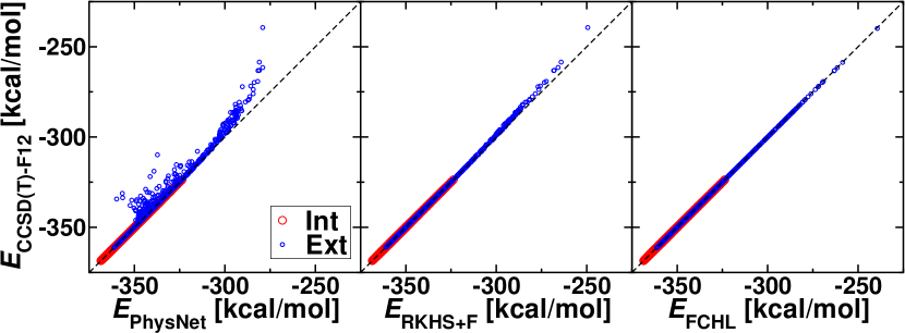
Figure 4: Comparison of the reference ab initio CCSD(T)-F12 energies ($y-$axis) with the machine-learned energies ($x-$axis) for formaldehyde geometries in Set2 (2500 structures). Here the models trained on the largest data set size of 3200 and having the smallest MAE($E$) were used. The data points are shown in two distinct colors (and sizes for clarity) for the CO, CH, and OH bonds which cover intervals in the training data set bracketed by [1.14, 1.28], [0.88, 1.40] and [1.83, 2.24] Å, respectively. The red symbols are for structures in which all distances are inside the range sampled in the training set (1333 structures) whereas the blue symbols is for all other structures (1167 structures). PhysNet (left panel) performs well for unknown structures covered by the training set but fails for structures outside. RKHS+F (middle panel) is very reliable for all structures in Set2 except for those with the highest energy and FCHL (right panel) predicts all geometries reliably.

The extrapolation data set (Set2) sampled at higher temperature than the training data set is examined and histograms for three bond lengths (C–O, C–H and O–H) are shown in Figures S1 to S3 for both the training and the extrapolation data set. It is apparent that structures contained in Set2 reach more distorted geometries and were never “seen” by the ML models. Figure 4 shows the comparison between the reference CCSD(T)-F12 and the machine-learned energies from models trained on the largest reference data set. The predictions from PhysNet either agree with the reference (indicated by the red circles on the black dashed line) or yield lower energies than the reference calculations. This is different for RKHS+F and FCHL which reliably (blue symbols in Figure 4) extrapolate to energies a factor of $\sim 3$ higher than the energy range covered by the training set (red symbols in Figure 4). The performance of FCHL is even better than that of RKHS+F. The MAEs and RMSEs of the three ML methods trained on different data set sizes and tested on Set2 are illustrated in Figure S5.

4.3 Vibrational Spectroscopy

[cm-1]	Exp	CCSD(T)-F12	RKHS+F	PhysNet	FCHL
$\nu_{1}$	2782.0	2933.8	2933.5	2932.9	2933.6
$\nu_{2}$	1746.0	1776.4	1776.4	1776.6	1776.4
$\nu_{3}$	1500.0	1532.7	1532.6	1532.0	1532.7
$\nu_{4}$	1167.0	1186.5	1186.4	1185.7	1186.5
$\nu_{5}$	2843.0	3005.8	3005.8	3004.3	3005.6
$\nu_{6}$	1249.0	1268.2	1268.1	1267.7	1268.2
RMSE		93.4	0.1	0.9	0.1

Table 1: Comparison of the normal mode frequencies obtained from the different ML models with their reference frequency (CCSD(T)-F12) and with those from experiment⁸. The frequency calculations were performed with the model trained on the largest data set of 3200 structures and having the lowest MAE($E$). The RMSEs between the experiment and the ab initio frequencies (CCSD(T)-F12) and between the ab initio reference frequencies and the ML predictions (RKHS+F, PhysNet and FCHL) are given.

Normal mode frequencies were determined at the CCSD(T)-F12 level of theory, see Table 1. Using the trained models on the largest reference data set ($N=3200$) the harmonic vibrations were calculated and are found to be in very close agreement with those from the quantum chemical calculations at the same level of theory. RMSEs of 0.14, 0.86 and 0.12 cm^-1 were found for RKHS+F, PhysNet and FCHL, respectively.

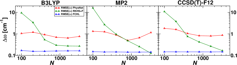
Figure 5: Performance curves showing RMSE $\Delta\omega$ for harmonic frequencies between the reference ab initio values and respective prediction using the PhysNet- (red), RKHS+F- (green) and FCHL- (blue) based models as a function of training set sizes. Left, mid, right panels correspond to training data from different levels of theory.

It is also of interest to determine harmonic frequencies from models with smaller training sets in order to assess whether there is a relationship between the accuracy of the machine-learned PES (see Figure 2) and a particular observable, here the normal mode frequency, see Figure 5. It is found that for PhysNet the accuracy with which the reference quantum chemical normal mode frequencies are predicted from the PhysNet-based PES are uniformly within $\sim 1$ cm^-1, independent on the size of the training set. Similarly, no data set size dependence is found for the FCHL frequency predictions which accurately reproduce the reference values with $\Delta\omega\sim 0.1$ cm^-1. The RKHS+F based predictions, however, show a $\Delta\omega\sim 10$ cm^-1 for the smallest training set size ($N=100$) and reach accuracies similar to the FCHL models for the largest training set sizes. In other words, all models are able to accurately predict the normal mode frequencies of H₂CO at all three levels of theory considered here but the number of training points $N$ to do may differ.

Infrared spectra from MD simulations further probe the regions around the minimum of the PES and provide an additional way to validate the trained ML-models. It is also possible to directly compare these spectra with experiments although for the high frequency modes it is known that the computed band positions can be inaccurate due to limited sampling of the anharmonicities because zero point vibrational energy is not included in classical MD simulations.^{55, 56, 57}

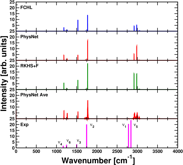
Figure 6: IR spectra from trajectories run on the different PESs. The trajectories from panels FCHL, PhysNet and RKHS+F were all started from the same initial conditions (geometry and momenta) corresponding to exactly 300 K. The RKHS+F method does not learn the molecular dipole moments and used PhysNet to predict the dipole moment of every snapshot along the RKHS+F trajectory. “PhysNet Ave” corresponds to the average over 1000 independent trajectories, each 200 ps in length. The trajectories are started from the same geometry but random momenta were drawn randomly from a Maxwell-Boltzmann distribution corresponding to 300 K. All simulations were run with the model trained on the largest data set of 3200 structures and having the lowest MAE($E$). The bottom panel reports the experimental infrared spectrum⁸ as a stick spectrum including intensities.

The IR spectra calculated from finite-$T$ MD simulations using the FCHL-, PhysNet- and RKHS+F-based approaches (blue, red and green, respectively) are shown in Figure 6. They all agree very well with the experimentally determined band positions, except for the CH stretching modes, and the relative intensities of the bands are also qualitatively correct. For direct comparison, all MD simulations were started from identical initial conditions. To improve convergence of the spectra, an average over all 1000 independent runs using PhysNet is also reported. It was found that even using random samples of 500 such spectra gives the same IR spectrum. Therefore, the averaged spectrum shown can be considered converged.

5 Discussion

The results indicate that all three ML-based approaches are successful in correctly describing the near-equilibrium region of the PES. The extrapolation capabilities of PhysNet are limited whereas RKHS+F and FCHL provide robust global PESs with FCHL showing the best performance, see Figure 4. For energy and force prediction and harmonic frequencies FCHL is best, followed by RKHS+F and PhysNet, specifically for larger data sets. However, it should be emphasized that the differences are generally small. For harmonic frequencies none of the models differs by more than 1 cm^-1 from the reference calculations, see Table 1.

Mode	PhysNet	CCSD(T)-F12	$\Delta$
$\nu_{1}$	2933.62	2933.79	0.17
$\nu_{2}$	1776.36	1776.39	0.03
$\nu_{3}$	1532.56	1532.70	0.14
$\nu_{4}$	1186.37	1186.46	0.09
$\nu_{5}$	3005.68	3005.81	0.13
$\nu_{6}$	1268.21	1268.17	0.04

Table 2: Harmonic frequencies in cm^-1 for a PhysNet model trained to convergence of the forces. All frequencies are within less than 0.2 cm^-1 of the reference CCSD(T)-F12 calculations, see also Table 1.

For the PhysNet-based approach a few more tests have been carried out. One of them concerns improving the harmonic frequencies ($\sim 1$ cm^-1 averaged difference compared with $\sim 0.1$ cm^-1 from the two kernel-based methods) by applying a slightly different learning protocol. For the PhysNet models presented above, training was stopped upon convergence of the energy predictions. Although further training would improve forces and dipole moments, the accuracy in the energy prediction would deteriorate because forces and energies are weighted differently in the loss function. Hence, an additional PhysNet model was trained on 3200 data points to convergence of the forces to investigate the accuracy of the harmonic frequencies. The results, reported in Table 2, are similar to those from RKHS+F and FCHL with an averaged RMSE of $\Delta\omega\approx 0.1$ cm^-1. On the other hand the MAE of the energy (predicting the test set) increased by approximately one order of magnitude to $\sim 4\cdot 10^{-3}$  kcal/mol, which is still very accurate. Hence, for obtaining accurate harmonic frequencies a good force-learned model can be advantageous.

As the harmonic frequencies differ quite substantially from the experimentally measured ones, it was also decided to compute the anharmonic frequencies from PhysNet by supplying energies, forces and the Hessian to the Gaussian09 quantum chemistry program. Because direct comparison with the ab initio values was not possible for the CCSD(T)-F12 level of theory, a comparison using the PhysNet MP2 model has been carried out and is reported in Table S5. The MP2 reference frequencies are reproduced with an RMSE of $\sim 1.0$ cm^-1 and the anharmonic values with an RMSE of $\sim 18.3$ cm^-1. Here, the largest deviations are found for the high-frequency modes (deviation of $\sim 30$ cm^-1). Note that the MP2 model was trained only up to the convergence of the energy and further training is expected to improve anharmonic frequencies as well. Table 3 compares the band centers from the finite-temperature IR spectra, the harmonic and anharmonic frequencies from using PhysNet and the experimental results. In particular for the stretch modes involving hydrogen atom motion (CH symmetric and antisymmetric stretch) the improvement for the anharmonic modes over harmonic frequencies and the MD simulations is remarkable. But all other modes are also in considerably better agreement with experiment with an RMSE of 10.8 cm^-1 between experiment and anharmonic calculations. As PhysNet is the least performing ML approach it is expected that similar calculations using RKHS+F and FCHL trained on CCSD(T)-F12 reference data will be equally good or even better.

mode	IR/PhysNet	G09/PhysNet H	G09/PhysNet AH	Exp8
$\nu_{1}$	2930.0	2932.9	2805.7	2782.0
$\nu_{2}$	1773.0	1777.0	1741.5	1746.0
$\nu_{3}$	1532.0	1532.8	1498.6	1500.0
$\nu_{4}$	1185.0	1186.0	1170.9	1167.0
$\nu_{5}$	2996.0	3004.1	2852.5	2843.0
$\nu_{6}$	1266.0	1268.3	1245.3	1249.0
RMSE	89.1	92.6	10.8

Table 3: Harmonic and anharmonic frequencies in cm^-1 for the optimized H₂CO structure compared with those from experiment ($\nu_{i}$)⁸. The harmonic (G09/PhysNet H) and anharmonic (G09/PhysNet AH) frequencies are calculated with Gaussian 09 using the PhysNet PES trained on 3200 CCSD(T)-F12 energies, forces and dipole moments. They are compared with IR center frequencies from experiment (Exp) and calculated from MD simulations (IR/PhysNet, see also Fig 6, PhysNet Ave). The RMSE between experiment and computations is shown in the last row.

The availability of PESs at different levels of theory also provides the opportunity to discuss shortcuts to high level of theory PES representations. Comparing B3LYP/cc-pVDZ energies (or predictions of PhysNet trained on B3LYP data, PhysNet_B3LYP) to CCSD(T)-F12/aug-cc-pVTZ-F12 energies illustrates a systematic shift as well as a regular scatter (see Fig. 7, black circles). Such correlations suggest that a combination of multiple levels of theory during training will be beneficial. In the following, “transfer learning” (TL) was used^{58, 59} although other methods, such as $\Delta$-Machine Learning ⁶⁰ (for kernel-based methods), multi-fidelity learning ⁶¹, or the multi-level grid combination technique ⁶² could also be used

Starting from a PhysNet model trained at a lower level of theory (B3LYP/cc-pVDZ), TL can be used to reach a higher level of theory (CCSD(T)-F12/aug-cc-pVTZ-F12) at little additional cost. Thus, the best B3LYP PhysNet model (as judged from the MAE($E$)) trained on 3200 H₂CO geometries is used as the reference and to initialize the parameters of the TL model. Different TL models were generated based on different training set sizes, with structures randomly chosen from Set1 of the CCSD(T)-F12 data set. The following data set sizes $N_{\rm tot}^{\rm TL}(N_{\rm train}^{\rm TL},N_{\rm valid}^{\rm TL})$ were considered for TL: 2(1,1), 10(9,1), 25(22,3), 50(45,5), 100(90,10), and 200(180,20).

The progress of TL PhysNet_B3LYP to CCSD(T)-F12 quality is illustrated in Figure 7. TL with $N_{\rm tot}^{\rm TL}=2$ (blue circles) suffices to eliminate the systematic shift between B3LYP and CCSD(T)-F12, whereas most of the scattered data points are corrected with $N_{\rm tot}^{\rm TL}=10$ (green circles). Note that chemical accuracy (RMSE($E$) better than 1 kcal/mol ) is achieved with as little as two additional points at the higher level of theory whereas a MAE($E{\rm)}=0.004$ kcal/mol and a RMSE($E$) = 0.006 kcal/mol is achieved with TL using $N_{\rm tot}^{\rm TL}=200$. The performance based on MAEs and RMSEs of the remaining data set sizes is summarized in Table S6 and illustrated as a learning curve in Figure S6.

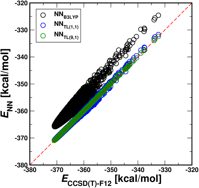
Figure 7: Correlation between the energy predicted by different PhysNet models and the CCSD(T)-F12 energies for the same molecular geometries. The black circles show the performance of the B3LYP PhysNet model to predict the CCSD(T)-F12 energies. The blue and green circles show the performance of the B3LYP model transfer learned with $N_{\rm tot}^{\rm TL}=2$ at the higher level of theory, respectively. Two structures suffice to eliminate the systematic shift whereas 10 structures where needed to reduce the scatter.

Another measure for the performance of the TL models is the quality of predicted normal mode frequencies compared with the CCSD(T)-F12 reference. For this the TL(180,20) model was used and the results are summarized in Table 4. This TL model reproduces the reference CCSD(T)-F12 frequencies to within $\sim 5$ cm^-1 or better. It is expected that a more careful selection of particular geometries (e.g. geometries with displacements along normal modes) will further improve the prediction with a smaller number of $N_{\rm tot}^{\rm TL}$ for accuracy as was recently shown for malonaldehyde.⁶³

mode	TL(180,20)	PhysNetCCSD(T)-F12	CCSD(T)-F12
$\nu_{1}$	2930.8	2932.9	2933.79
$\nu_{2}$	1777.0	1776.6	1776.39
$\nu_{3}$	1529.9	1532.0	1532.70
$\nu_{4}$	1179.1	1185.7	1186.46
$\nu_{5}$	3000.9	3004.3	3005.81
$\nu_{6}$	1266.3	1267.7	1268.17

Table 4: Normal mode frequencies predicted by the transfer learned model TL(180,20) in comparison to a PhysNet trained on 3200 CCSD(T)-F12 data points and with the ab initio CCSD(T)-F12 frequencies.

6 Conclusions

We have investigated and compared the application of kernel and neural network based ML models capable of generating fully dimensional PESs for formaldehyde, and their application to vibrational spectroscopy. Training/Test-set consistency runs indicate that the ML models achieve such precision that noise levels even in unseen data can be detected. We find it reassuring that all three ML models considered, despite their differences in representation, functional form and number of coefficients, result in overall excellent performance. In particular, they are also applicable to extrapolation regimes, and demonstrably useful for predicting experimental observables such as IR spectra. With regards to the actual representation of atoms in molecules, one can consider FCHL as intermediate between “no representation” (RKHS+F) and a machine-learned representation (PhysNet). Moreover, TL of PhysNet was demonstrated to result in substantial improvements in data-efficiency. We expect our findings for machine learning of high-quality PESs and harmonic frequency prediction to also extend to larger molecules as has been recently demonstrated for PhysNet^{63, 64} and molecules with up to 10 atoms using RKHS+F.²¹

Supporting Information

The supporting information reports the optimized structures of the three learned models, histograms for bond lengths of Set1 and Set2, additional learning curves and harmonic and anharmonic frequencies at the MP2 level.

Data Availability Statement

The machine-learning codes and documentation for training PhysNet, FCHL, and RKHS+F-based models are available at https://github.com/MMunibas/PhysNet, https://github.com/qmlcode/qml, and https://github.com/MMunibas/RKHS_CH2O and the reference data can be downloaded from zenodo https://doi.org/10.5281/zenodo.3923823.

References

- Behler 2016 Behler, J. Perspective: Machine learning potentials for atomistic simulations. J. Chem. Phys. 2016, 145, 170901
- Von Lilienfeld 2018 Von Lilienfeld, O. A. Quantum machine learning in chemical compound space. Angew. Chem. Int. Ed. 2018, 57, 4164–4169
- Butler et al. 2018 Butler, K. T.; Davies, D. W.; Cartwright, H.; Isayev, O.; Walsh, A. Machine learning for molecular and materials science. Nature 2018, 559, 547–555
- Koner et al. 2020 Koner, D.; Salehi, S. M.; Mondal, P.; Meuwly, M. Non-conventional force fields for applications in spectroscopy and chemical reaction dynamics. J. Chem. Phys. 2020, in print, in print
- Zhang et al. 2004 Zhang, X.; Zou, S.; Harding, L. B.; Bowman, J. M. A global ab initio potential energy surface for formaldehyde. J. Phys. Chem. A 2004, 108, 8980–8986
- Wang et al. 2017 Wang, X.; Houston, P. L.; Bowman, J. M. A new (multi-reference configuration interaction) potential energy surface for H2CO and preliminary studies of roaming. Philos. Trans. R. Soc. A 2017, 375, 20160194
- Karton et al. 2006 Karton, A.; Rabinovich, E.; Martin, J. M.; Ruscic, B. W4 theory for computational thermochemistry: In pursuit of confident sub-kJ/mol predictions. J. Chem. Phys. 2006, 125, 144108
- Herndon et al. 2005 Herndon, S. C.; Nelson Jr, D. D.; Li, Y.; Zahniser, M. S. Determination of line strengths for selected transitions in the band relative to the and bands of H2CO. J. Quant. Spectrosc. Radiat. Transf. 2005, 90, 207–216
- Franz et al. 2016 Franz, A. W.; Kronemayer, H.; Pfeiffer, D.; Pilz, R. D.; Reuss, G.; Disteldorf, W.; Gamer, A. O.; Hilt, A. Ullmann’s Encyclopedia of Industrial Chemistry; American Cancer Society, 2016; pp 1–34
- Authority 2014 Authority, E. F. S. Endogenous formaldehyde turnover in humans compared with exogenous contribution from food sources. EFSA J 2014, 12, 3550–3560
- Wang et al. 2017 Wang, C.; Huang, X.-F.; Han, Y.; Zhu, B.; He, L.-Y. Sources and potential photochemical roles of formaldehyde in an urban atmosphere in South China. J. Geophys. Res. Atmos. 2017, 122, 11934–11947
- Zhang 2018 Zhang, L. Formaldehyde: Exposure, Toxicity and Health Effects; Royal Society of Chemistry, 2018; Vol. 37
- Snyder et al. 1969 Snyder, L. E.; Buhl, D.; Zuckerman, B.; Palmer, P. Microwave detection of interstellar formaldehyde. Phys. Rev. Lett. 1969, 22, 679–681
- Townsend et al. 2004 Townsend, D.; Lahankar, S. A.; Lee, S. K.; Chambreau, S. D.; Suits, A. G.; Zhang, X.; Rheinecker, J.; Harding, L.; Bowman, J. M. The roaming atom: straying from the reaction path in formaldehyde decomposition. Science 2004, 306, 1158–1161
- Becke 1993 Becke, A. D. Becke’s three parameter hybrid method using the LYP correlation functional. J. Chem. Phys. 1993, 98, 5648–5652
- Lee et al. 1988 Lee, C.; Yang, W.; Parr, R. G. Development of the Colle-Salvetti correlation-energy formula into a functional of the electron density. Phys. Rev. B 1988, 37, 785–789
- Møller and Plesset 1934 Møller, C.; Plesset, M. S. Note on an approximation treatment for many-electron systems. Phys. Rev. 1934, 46, 618–622
- Adler et al. 2007 Adler, T. B.; Knizia, G.; Werner, H.-J. A simple and efficient CCSD (T)-F12 approximation. J. Chem. Phys. 2007, 127, 221106
- Ho and Rabitz 1996 Ho, T.-S.; Rabitz, H. A General Method for Constructing Multidimensional Molecular Potential Energy Surfaces from Ab Initio Calculations. J. Chem. Phys. 1996, 104, 2584–2597
- Unke and Meuwly 2017 Unke, O. T.; Meuwly, M. Toolkit for the Construction of Reproducing Kernel-Based Representations of Data: Application to Multidimensional Potential Energy Surfaces. J. Chem. Inf. and Mod. 2017, 57, 1923–1931
- Koner and Meuwly 2020 Koner, D.; Meuwly, M. Permutationally Invariant, Reproducing Kernel-Based Potential Energy Surfaces for Polyatomic Molecules: From Formaldehyde to Acetone. arXiv e-prints 2020, arXiv:2005.04667
- Unke and Meuwly 2019 Unke, O. T.; Meuwly, M. PhysNet: A Neural Network for Predicting Energies, Forces, Dipole Moments, and Partial Charges. J. Chem. Theory Comput. 2019, 15, 3678–3693
- Faber et al. 2018 Faber, F. A.; Christensen, A. S.; Huang, B.; von Lilienfeld, O. A. Alchemical and structural distribution based representation for universal quantum machine learning. J. Chem. Phys. 2018, 148, 241717
- Gilmer et al. 2017 Gilmer, J.; Schoenholz, S. S.; Riley, P. F.; Vinyals, O.; Dahl, G. E. Neural message passing for quantum chemistry. Proceedings of the 34th International Conference on Machine Learning-Volume 70. 2017; pp 1263–1272
- Baydin et al. 2017 Baydin, A. G.; Pearlmutter, B. A.; Radul, A. A.; Siskind, J. M. Automatic differentiation in machine learning: a survey. J. Mach. Learn. Res. 2017, 18, 5595–5637
- Kingma and Ba 2014 Kingma, D. P.; Ba, J. Adam: A Method for Stochastic Optimization. arXiv e-prints 2014, arXiv:1412.6980
- Aronszajn 1950 Aronszajn, N. Theory of Reproducing Kernels. Trans. Amer. Math. Soc. 1950, 68, 337–404
- Christensen et al. 2020 Christensen, A. S.; Bratholm, L. A.; Faber, F. A.; Anatole von Lilienfeld, O. FCHL revisited: Faster and more accurate quantum machine learning. J. Chem. Phys. 2020, 152, 044107
- Schölkopf et al. 2001 Schölkopf, B.; Herbrich, R.; Smola, A. J. A Generalized Representer Theorem. International Conference on Computational Learning Theory. 2001; pp 416–426
- Golub and Van Loan 2012 Golub, G. H.; Van Loan, C. F. Matrix Computations; JHU Press Baltimore, 2012; Vol. 3
- Soldan and Hutson 2000 Soldan, P.; Hutson, J. On the long-range and short-range behavior of potentials from reproducing kernel Hilbert space interpolation. J. Chem. Phys. 2000, 112, 4415–4416
- Faber et al. 2017 Faber, F. A.; Hutchison, L.; Huang, B.; Gilmer, J.; Schoenholz, S. S.; Dahl, G. E.; Vinyals, O.; Kearnes, S.; Riley, P. F.; von Lilienfeld, O. A. Prediction Errors of Molecular Machine Learning Models Lower than Hybrid DFT Error. J. Chem. Theory Comput. 2017, 13, 5255–5264
- Bartók et al. 2010 Bartók, A. P.; Payne, M. C.; Kondor, R.; Csányi, G. Gaussian Approximation Potentials: The Accuracy of Quantum Mechanics, without the Electrons. Phys. Rev. Lett. 2010, 104, 136403
- Hansen et al. 2015 Hansen, K.; Biegler, F.; von Lilienfeld, O. A.; Müller, K.-R.; Tkatchenko, A. Interaction potentials in molecules and non-local information in chemical space. J. Phys. Chem. Lett. 2015, 6, 2326–2331
- Bartók and Csányi 2015 Bartók, A. P.; Csányi, G. Gaussian approximation potentials: A brief tutorial introduction. Int. J. Quantum Chem. 2015, 115, 1051–1057
- Rasmussen and Williams 2006 Rasmussen, C. E.; Williams, C. K. I. Gaussian Processes for Machine Learning, www.GaussianProcess.org; MIT Press: Cambridge, 2006; Editor: T. Dietterich
- Mathias 2015 Mathias, S. A Kernel-Based Learning Method for an efficient Approximation of the high-dimensional Born-Oppenheimer Potential Energy Surface. M.Sc. thesis, Mathematisch-Naturwissenschaftliche Fakultät der Rheinischen Friedrich-Wilhelms-Universität Bonn, Germany, 2015; \urlhttp://wissrech.ins.uni-bonn.de/teaching/master/masterthesis_mathias_revised.pdf; accessed February 2020
- Christensen et al. 2019 Christensen, A. S.; Faber, F. A.; von Lilienfeld, O. A. Operators in quantum machine learning: Response properties in chemical space. J. Chem. Phys. 2019, 150, 064105
- von Lilienfeld et al. 2015 von Lilienfeld, O. A.; Ramakrishnan, R.; Rupp, M.; Knoll, A. Fourier series of atomic radial distribution functions: A molecular fingerprint for machine learning models of quantum chemical properties. Int. J. Quantum Chem. 2015, 115, 1084–1093
- Gasteiger and Marsili 1980 Gasteiger, J.; Marsili, M. Iterative partial equalization of orbital electronegativity—a rapid access to atomic charges. Tetrahedron 1980, 36, 3219–3228
- O’Boyle et al. 2011 O’Boyle, N. M.; Banck, M.; James, C. A.; Morley, C.; Vandermeersch, T.; Hutchison, G. R. Open Babel: An open chemical toolbox. J. Cheminf. 2011, 3, 33
- Dunning Jr 1989 Dunning Jr, T. H. Gaussian basis sets for use in correlated molecular calculations. I. The atoms boron through neon and hydrogen. J. Chem. Phys. 1989, 90, 1007–1023
- Neese 2012 Neese, F. The ORCA program system. WIREs Comput. Mol. Sci. 2012, 2, 73–78
- Kendall et al. 1992 Kendall, R. A.; Dunning Jr, T. H.; Harrison, R. J. Electron affinities of the first-row atoms revisited. Systematic basis sets and wave functions. J. Chem. Phys. 1992, 96, 6796–6806
- Peterson et al. 2008 Peterson, K. A.; Adler, T. B.; Werner, H.-J. Systematically convergent basis sets for explicitly correlated wavefunctions: The atoms H, He, B–Ne, and Al–Ar. J. Chem. Phys. 2008, 128, 084102
- Werner et al. 2019 Werner, H.-J.; Knowles, P. J.; Knizia, G.; Manby, F. R.; Schütz, M.; Celani, P.; Györffy, W.; Kats, D.; Korona, T.; Lindh, R. et al. MOLPRO, version 2019.2, a package of ab initio programs. 2019
- Smith et al. 2017 Smith, J. S.; Isayev, O.; Roitberg, A. E. ANI-1, A data set of 20 million calculated off-equilibrium conformations for organic molecules. Sci. Data 2017, 4, 170193
- Larsen et al. 2017 Larsen, A. H.; Mortensen, J. J.; Blomqvist, J.; Castelli, I. E.; Christensen, R.; Dułak, M.; Friis, J.; Groves, M. N.; Hammer, B.; Hargus, C. et al. The atomic simulation environment—a Python library for working with atoms. J. Phys. Condens. Matter 2017, 29, 273002
- Pernot et al. 2020 Pernot, P.; Huang, B.; Savin, A. Impact of non-normal error distributions on the benchmarking and ranking of Quantum Machine Learning models. arXiv e-prints 2020, arXiv:2004.02524
- Gyorffy and Werner 2018 Gyorffy, W.; Werner, H.-J. Analytical energy gradients for explicitly correlated wave functions. II. Explicitly correlated coupled cluster singles and doubles with perturbative triples corrections: CCSD(T)-F12. J. Chem. Phys. 2018, 148, 114104
- Mackerell 2004 Mackerell, A. D. Empirical force fields for biological macromolecules: Overview and issues. J. Comput. Chem. 2004, 25, 1584–1604
- Kramer et al. 2012 Kramer, C.; Gedeck, P.; Meuwly, M. Atomic multipoles: Electrostatic potential fit, local reference axis systems, and conformational dependence. J. Comput. Chem. 2012, 33, 1673–1688
- Bereau et al. 2013 Bereau, T.; Kramer, C.; Meuwly, M. Leveraging Symmetries of Static Atomic Multipole Electrostatics in Molecular Dynamics Simulations. J. Chem. Theory Comput. 2013, 9, 5450–5459
- Koner et al. 2019 Koner, D.; Veliz, J. C. S. V.; van der Avoird, A.; Meuwly, M. Near dissociation states for H-He on MRCI and FCI potential energy surfaces. Phys. Chem. Chem. Phys. 2019, 21, 24976–24983
- Qu and Bowman 2018 Qu, C.; Bowman, J. M. IR Spectra of (HCOOH)2 and (DCOOH)2: Experiment, VSCF/VCI, and Ab Initio Molecular Dynamics Calculations Using Full-Dimensional Potential and Dipole Moment Surfaces. J. Phys. Chem. Lett 2018, 9, 2604–2610
- Qu and Bowman 2018 Qu, C.; Bowman, J. M. Quantum and classical IR spectra of (HCOOH)2,(DCOOH)2 and (DCOOD)2 using ab initio potential energy and dipole moment surfaces. Faraday Discuss 2018, 212, 33–49
- Xu and Meuwly 2017 Xu, Z.-H.; Meuwly, M. Vibrational Spectroscopy and Proton Transfer Dynamics in Protonated Oxalate. J. Phys. Chem. A 2017, 121, 5389–5398
- Taylor and Stone 2009 Taylor, M. E.; Stone, P. Transfer learning for reinforcement learning domains: A survey. J. Mach. Learn. Res. 2009, 10, 1633–1685
- Pan and Yang 2009 Pan, S. J.; Yang, Q. A survey on transfer learning. IEEE Trans. Knowl. Data Eng. 2009, 22, 1345–1359
- Ramakrishnan et al. 2015 Ramakrishnan, R.; Dral, P.; Rupp, M.; von Lilienfeld, O. A. Big Data meets Quantum Chemistry Approximations: The -Machine Learning Approach. J. Chem. Theory Comput. 2015, 11, 2087–2096
- Batra et al. 2019 Batra, R.; Pilania, G.; Uberuaga, B. P.; Ramprasad, R. Multifidelity Information Fusion with Machine Learning: A Case Study of Dopant Formation Energies in Hafnia. ACS Appl. Mater. Interfaces 2019, 11, 24906–24918
- Zaspel et al. 2018 Zaspel, P.; Huang, B.; Harbrecht, H.; von Lilienfeld, O. A. Boosting quantum machine learning models with a multilevel combination technique: Pople diagrams revisited. jctc 2018, 15, 1546–1559
- Käser et al. 2020 Käser, S.; Unke, O. T.; Meuwly, M. Reactive Dynamics and Spectroscopy of Hydrogen Transfer from Neural Network-Based Reactive Potential Energy Surfaces. New J. Phys. 2020, 22, 055002
- Käser et al. 2020 Käser, S.; Unke, O. T.; Meuwly, M. Isomerization and decomposition reactions of acetaldehyde relevant to atmospheric processes from dynamics simulations on neural network-based potential energy surfaces. J. Chem. Phys. 2020, 152, 214304