Theoretical and observational constraints on regularized 4$D$ Einstein-Gauss-Bonnet gravity

Abstract

Regularized Einstein-Gauss-Bonnet (EGB) theory of gravity in four dimensions is a new attempt to include nontrivial contributions of Gauss-Bonnet term. In this paper, we make a detailed analysis on possible constraints of the model parameters of the theory from recent cosmological observations, and some theoretical constraints as well. Our results show that the theory with vanishing bare cosmological constant, $\Lambda_{0}$, is ruled out by the current observational value of $w_{de}$, and the observations of GW170817 and GRB 170817A as well. For nonvanishing bare cosmological constant, instead, our results show that the current observation of the speed of GWs measured by GW170817 and GRB 170817A would place a constraints on $\tilde{\alpha}$, a dimensionless parameter of the theory, as $-7.78\times 10^{-16}\leq\tilde{\alpha}\leq 3.33\times 10^{-15}$.

I Introduction

The first detection of gravitational waves (GWs) by LIGO/Virgo GW150914 begins to have a profound impact on our understanding of the nature. They provide new powerful ways to explore physics of the Universe. GW170817 TheLIGOScientific:2017qsa , the first detected GW event with electromagnetic counterparts, extensively enriched the ways. From then on, a new era of multi-messenger GW astronomy has began. Fermi Gamma-Ray Burst Monitor Goldstein:2017mmi and the International Gamma-Ray Astrophysics Laboratory Savchenko:2017ffs observed a gamma ray burst GRB 170817A after $1.74\pm 0.05$s, on which a range of constraint on the speed of GWs can be obtained. Particularly, with the assumption that the GW signal was emitted at most 10s before the GRB signal, one can obtain a bound on the velocity of the GWs, namely, $-3\times 10^{-15}\leq\frac{c_{\rm gw}}{c}-1\leq 7\times 10^{-16}$ Monitor:2017mdv .

The observations of GW events GW150914 ; Abbott:2016nmj ; Abbott:2017vtc ; Abbott:2017gyy ; Abbott:2017oio ; TheLIGOScientific:2017qsa in recent years, of course, support the validity of Einstein’s theory enough. However, whether alternative theories of gravity which can do equally well as Einstein’s theory can be constructed or not? This point has attracted a large number of researchers to study, such as scalar-tensor theories Horndeski:1974wa ; Fujii:2003pa ; Chow:2009fm ; Tsujikawa:2010zza ; Chen:2010va ; Clifton:2011jh ; Gleyzes:2014qga ; Crisostomi:2016czh ; Sakstein:2017xjx ; Ezquiaga:2017ekz ; Green:2017qcv ; Casalino:2018wnc , vector-tensor theories Baker:2017hug , and so on. With more and more GW events to be detected in the future, it is expected that constraints on the speed of GWs will be more and more stringent. This makes it an effective tool to test the alternative theories of gravity Mirshekari:2011yq ; Jimenez:2015bwa ; Chesler:2017khz ; Baker:2017hug ; Creminelli:2017sry ; Sakstein:2017xjx ; Ezquiaga:2017ekz ; Green:2017qcv ; Nishizawa:2017nef ; Arai:2017hxj ; Battye:2018ssx .

Hence, we are paying attention to modified theories of gravity. One of the most elegant modifications is the Einstein-Gauss-Bonnet gravity. It is generally discussed that the extension of higher derivatives by adding the polynomial invariants of the Riemann tensor to the Einstein-Hilbert action is admitted in Einstein’s gravity. The field equations which involve four derivatives may lead to renormalizability, while the theory contains an inevitable ghostlike massive graviton Stelle:1976gc . It was found that the Gauss-Bonnet(GB) term, which is a quadratic combination of the Riemann curvature tensor, keeps the equations at second-order in the metric and hence is free of the ghost Lovelock:1971yv ; Zumino:1985dp . In four or lower dimensions, however, these specific combinations of tensor polynomials either vanish or become total derivative. The trivialness in four dimensions excludes it as a more realistic model.

In Glavan:2019inb , a new theory called 4 dimensional Einstein-Gauss-Bonnet ($4D$ EGB) gravity was proposed. It considers a $D\to 4$ limit of the D-dimensional Gauss-Bonnet gravity by rescaling the GB dimensional coupling constant $\alpha\to\hat{\alpha}/(D-4)$. The idea is to introduce the divergent coefficient to cancel the vanishing contribution of $\mathcal{G}$ in four dimensions, in a manner that is conceptually similar to the dimensional regularization procedure used in quantum field theories. The goal of this is to produce a nontrivial gravity theory in four dimensions that includes a non-vanishing contribution from the Gauss-Bonnet term. A large number of relevant works has been done in the past few months Nojiri:2020tph ; Konoplya:2020bxa ; Guo:2020zmf ; Fernandes:2020rpa ; Casalino:2020kbt ; Konoplya:2020qqh ; Hegde:2020xlv ; Ghosh:2020vpc ; Doneva:2020ped ; Zhang:2020qew ; Konoplya:2020ibi ; Singh:2020xju ; Ghosh:2020syx ; Konoplya:2020juj ; Kumar:2020uyz ; Zhang:2020qam ; HosseiniMansoori:2020yfj ; Wei:2020poh ; Singh:2020nwo ; Churilova:2020aca ; Islam:2020xmy ; Mishra:2020gce ; Kumar:2020xvu ; Liu:2020vkh ; EGB29 ; Konoplya:2020cbv ; Heydari-Fard:2020sib ; Jin:2020emq ; Zhang:2020sjh ; EslamPanah:2020hoj ; Aragon:2020qdc ; Yang:2020czk ; Lin:2020kqe ; Yang:2020jno ; Narain:2020qhh ; Narain:2020tsw ; Ge:2020tid ; Banerjee:2020dad . However, the resulting theory has been questioned a lot. The theory is found to be not well defined in the limit $D\rightarrow 4$ Ai:2020peo ; Gurses:2020ofy ; Lu:2020iav ; Kobayashi:2020wqy ; Hennigar:2020lsl ; Fernandes:2020nbq ; Mahapatra:2020rds . Moreover, the vacua of the model are unstable or ill-defined too shu . To overcome this, several regularization schemes have been proposed Lu:2020iav ; Kobayashi:2020wqy ; Hennigar:2020lsl ; Fernandes:2020nbq ; Aoki:2020iwm . This generally leads to a scalar-tensor gravity, being a subclass of Hordenski theories VanAcoleyen:2011mj .

In this work, we will perform a detailed analysis of cosmological perturbations of the regularized model around the FRW universe. The speed of tensor modes can be read off from these perturbative equations. Then we look for possible constraints on the coupling constant $\hat{\alpha}$ of the regularized model through latest observational constraints on the speed of GWs from GW170817 TheLIGOScientific:2017qsa and GRB 170817A Monitor:2017mdv . Our results show that, for the theory with the bare cosmological constant $\Lambda_{0}=0$, there are two contradictions: one is the theoretical requirements of the model are contradicted with the current observational value of $w_{de}$. The other is the constraints imposed from GW170817 and GRB 170817A disagree with the current cosmological constraint on the ratio of energy densities between dark energy and matter, $\frac{\Omega_{de}}{\Omega_{m}}$. Therefore, the theory $\Lambda_{0}=0$ is ruled out. The case with $\Lambda_{0}\neq 0$, however, receives a constraint from the speed of GWs measured by GW170817 and GRB 170817A, explicitly, $-7.78\times 10^{-16}\leq\tilde{\alpha}\leq 3.33\times 10^{-15}$. To see whether the scalar perturbations will give more stringent constrains or not, we discuss scalar perturbations as well.

The rest of the paper is organized as follows. In section II, we briefly review the regularized Einstein-Gauss-Bonnet theory in $4$ dimensions with cosmological constant. After applying it to the FRW universe, a set of dynamical equations are obtained, followed by a set of cosmological solutions. In section III, we perform linear perturbation analysis around FRW background. The quadratic action and the velocity of gravitation waves are obtained. In section IV, we apply the observational constraints from GW170817 and GRB 170817A to restrict the coupling constant $\hat{\alpha}$ of the model. In section V, the constrains from the scalar perturbations which may be more stringent are discussed as well. A brief concluding remark is drawn in the last section.

II Regularized Einstein-Gauss-Bonnet Theory in Four Dimensions

The action of Einstein-Gauss-Bonnet theory in $D$ dimensions with cosmological constant is

$$S = \int_{\mathcal{M}}\mathrm{d}^{D}x\sqrt{-g}\left(\ R-2\Lambda_{0}+\alpha\mathcal{G}\right)+S_{m},$$ (1)

where $\alpha$ is a coupling constant, $S_{m}$ is the action associated with matter field, and the Gauss-Bonnet term is

$$\mathcal{G} = R^{2}-4R_{\mu\nu}R^{\mu\nu}+R_{\mu\nu\alpha\beta}R^{\mu\nu\alpha\beta}~{}.$$ (2)

The idea of Glavan:2019inb is to construct a nontrivial theory by considering a replacement $\alpha\to\frac{\hat{\alpha}}{(D-4)}$. This, however, turns out to be questionable in many aspects. In particular, it was found the theory defined in this way has no well-defined limit Ai:2020peo ; Gurses:2020ofy ; Lu:2020iav ; Kobayashi:2020wqy ; Hennigar:2020lsl ; Fernandes:2020nbq ; shu . The way to fix this pathology is to perform a regularization. There are several regularization schemes in the literatures, such as the Kaluza–Klein-reduction procedure Lu:2020iav ; Kobayashi:2020wqy , the conformal subtraction procedure Hennigar:2020lsl ; Fernandes:2020nbq , and ADM decomposition analysis Aoki:2020iwm . The first two approaches give rise to the same regularized action, which is of the following form

$$S=\int_{\mathcal{M}}\mathrm{d}^{4}x\sqrt{-g}\Big{[} R -2\Lambda_{0}+\hat{\alpha}\Big{(}4G^{\mu\nu}\nabla_{\mu}\phi\nabla_{\nu}\phi-\phi\mathcal{G}$$

$$+4\Box\phi(\nabla\phi)^{2}+2(\nabla\phi)^{4}\Big{)}\Big{]}+S_{m},$$

where $\phi$ is a scalar field inherent from $D$ dimensions. It is introduced by Kaluza–Klein reduction of the metric Lu:2020iav ; Kobayashi:2020wqy

$$\mathrm{d}s_{D}^{2}=\mathrm{d}s_{4}^{2}+e^{2\phi}\mathrm{d}\Omega_{D-4}^{2},$$

or by conformal subtraction Hennigar:2020lsl ; Fernandes:2020nbq where the subtraction background is defined under a conformal transformation $g_{ab}\rightarrow e^{2\phi}g_{ab}$.

Varying with respect to the metric, we can get the field equations

$$G_{\mu\nu}+\Lambda_{0}g_{\mu\nu}=\hat{\alpha}\hat{\mathcal{H}}_{\mu\nu}+T_{\mu\nu}^{(m)},$$ (4)

where $T_{\mu\nu}^{(m)}$ is the energy-momentum tensor of the matter field, considering the matter context of the universe is a perfect fluid, so that the energy-momentum tensor take the form Carroll:2004st

$$T_{\mu\nu}^{(m)} = (\rho_{m}+p_{m})U_{\mu}U_{\nu}+p_{m}g_{\mu\nu},$$ (5)

where $\rho_{m}$, $p_{m}$ and $U_{\mu}$ are respectively energy density, pressure and four-velocity of the fluid. And

$$\hat{\mathcal{H}}_{\mu\nu} = 2R\big{(}\nabla_{\mu}\nabla_{\nu}\phi-\nabla_{\mu}\phi\nabla_{\nu}\phi\big{)}+2G_{\mu\nu}\Big{(}\big{(}\nabla\phi\big{)}^{2}-2\Box\phi\Big{)}+4G_{\nu\alpha}\big{(}\nabla^{\alpha}\nabla_{\mu}\phi-\nabla^{\alpha}\phi\nabla_{\mu}\phi\big{)}$$

$$+4G_{\mu\alpha}\big{(}\nabla^{\alpha}\nabla_{\nu}\phi-\nabla^{\alpha}\phi\nabla_{\nu}\phi\big{)}+4R_{\mu\alpha\nu\beta}\big{(}\nabla^{\beta}\nabla^{\alpha}\phi-\nabla^{\alpha}\phi\nabla^{\beta}\phi\big{)}$$

$$+4\nabla_{\alpha}\nabla_{\nu}\phi\big{(}\nabla^{\alpha}\phi\nabla_{\mu}\phi-\nabla^{\alpha}\nabla_{\mu}\phi\big{)}+4\nabla_{\alpha}\nabla_{\mu}\phi\nabla^{\alpha}\phi\nabla_{\nu}\phi-4\nabla_{\mu}\phi\nabla_{\nu}\phi\Big{(}\big{(}\nabla\phi\big{)}^{2}+\Box\phi\Big{)}$$

$$+4\Box\phi\nabla_{\nu}\nabla_{\mu}\phi-g_{\mu\nu}\Big{[}2R\big{(}\Box\phi-(\nabla\phi)^{2}\big{)}+4G^{\alpha\beta}\big{(}\nabla_{\beta}\nabla_{\alpha}\phi-\nabla_{\alpha}\phi\nabla_{\beta}\phi\big{)}+2\big{(}\Box\phi\big{)}^{2}$$

$$-\big{(}\nabla\phi\big{)}^{4}+2\nabla_{\beta}\nabla_{\alpha}\phi\big{(}2\nabla^{\alpha}\phi\nabla^{\beta}\phi-\nabla^{\beta}\nabla^{\alpha}\phi\big{)}\Big{]}$$

By varying with respect to the scalar field, we get

$$\frac{1}{8}\mathcal{G} = R^{\mu\nu}\nabla_{\mu}\phi\nabla_{\nu}\phi-G^{\mu\nu}\nabla_{\mu}\nabla_{\nu}\phi-\Box\phi(\nabla\phi)^{2}$$

$$+(\nabla_{\mu}\nabla_{\nu}\phi)^{2}-(\Box\phi)^{2}-2\nabla_{\mu}\phi\nabla_{\nu}\phi\nabla^{\mu}\nabla^{\nu}\phi$$

The trace of the field equations (4) is found to satisfy

$$R+\frac{\hat{\alpha}}{2}\mathcal{G}-4\Lambda_{0}=-T,$$ (8)

where $T=-\rho_{m}+3p_{m}$.

Assuming that the line-element describing by spatially-flat Friedmann-Robertson-Walker (FRW) metric is

$$\mathrm{d}s^{2}=-\mathrm{d}t^{2}+a^{2}(t)(\mathrm{d}x^{2}_{1}+\mathrm{d}x^{2}_{2}+\mathrm{d}x^{2}_{3}),$$ (9)

then taking a direct calculation, we show that the equations of motion become

$$3H^{2} = \rho_{GB}+\rho_{m}+\rho_{\Lambda},$$

$$2\dot{H}+3H^{2} = -p_{GB}-p_{m}-p_{\Lambda},$$ (10)

where the energy density, pressure of the GB term and the cosmological constant term are defined as

$$\rho_{GB} \equiv \Big{(}3\dot{\phi}^{4}+12\dot{\phi}^{3}H+18\dot{\phi}^{2}H^{2}+12\dot{\phi}H^{3}\Big{)}\hat{\alpha},$$

$$p_{GB} \equiv \Big{[}\dot{\phi}^{4}-4\dot{\phi}^{2}\ddot{\phi}-4\dot{\phi}^{2}(\dot{H}+H^{2})-2\dot{\phi}^{2}H^{2}$$

$$-8\dot{\phi}\ddot{\phi}H-8\dot{\phi}\big{(}\dot{H}+H^{2}\big{)}H-4\ddot{\phi}H^{2}\Big{]}\hat{\alpha},$$

$$\rho_{\Lambda} \equiv \Lambda_{0},$$

$$p_{\Lambda} \equiv -\Lambda_{0}.$$ (11)

And the scalar field equation, which is equivalent to $\nabla^{\mu}\hat{\mathcal{H}}_{\mu\nu}=0$ , reduces to,

$$\partial_{t}[(a\dot{\phi}+\dot{a})^{2}]=0,$$ (12)

which can be solved simply by

$$\dot{\phi} = -H,$$ (13)

or

$$\dot{\phi} = -H+\frac{A}{a},$$ (14)

where $H$ is the Hubble parameter, dot denotes derivative with respect to $t$, $A$ is the integration constant. It is obvious that these solutions are similar with Lu:2020iav ; Kobayashi:2020wqy .

III The speed of gravitational waves

To study the gravitational waves, let us consider the linear tensor perturbations of the FRW metric,

$$\mathrm{d}s^{2}=-\mathrm{d}t^{2}+a^{2}\left(t\right)\left(\delta_{ij}+h_{ij}\right)\mathrm{d}x^{i}\mathrm{d}x^{j},$$ (15)

where the tensor $h_{ij}$ satisfies the transverse-traceless condition, $\partial^{i}h_{ij}=0=\delta^{ij}h_{ij}$. Then the linear order field equation of $h_{ij}$ can be expressed as

$$\beta_{1}\ddot{h}_{ij}+\left(\dot{\beta_{1}}+3H\beta_{1}\right)\dot{h}_{ij}-\beta_{2}\frac{\vec{\nabla}^{2}}{a^{2}}h_{ij}=0.$$ (16)

The coefficients $\beta_{1}$ and $\beta_{2}$ are defined as

$$\beta_{1}\equiv 1-2\hat{\alpha}\dot{\phi}^{2}-4\hat{\alpha}\dot{\phi}H,$$ (17)

$$\beta_{2}\equiv 1+2\hat{\alpha}\dot{\phi}^{2}-4\hat{\alpha}\ddot{\phi}.$$ (18)

The corresponding quadratic action is

$$S_{h}=\int\mathrm{d}t\mathrm{d}^{3}xa^{3}\left[\beta_{1}\dot{h}_{ij}^{2}-\frac{\beta_{2}}{a^{2}}\left(\vec{\nabla}h_{ij}\right)^{2}\right].$$ (19)

To avoid ghost and gradient instability Kobayashi:2019hrl , the two coefficients $\beta_{1}$ and $\beta_{2}$ should be positive, namely, $\beta_{1}>0$ and $\beta_{2}>0$. This imposes constraints on the coupling constant $\hat{\alpha}$, and we will recall these constraints in next section.

It is more convenient to make the Fourier transformation and write the tensor perturbation $h_{ij}(\vec{x},t)$ as

$$h_{ij}(\vec{x},t)=\int\frac{\mathrm{d}^{3}k}{(2\pi)^{3}}\left[h_{k}^{+}\left(t\right)A^{+}_{ij}+h_{k}^{\times}\left(t\right)A^{\times}_{ij}\right]\exp\left(i\vec{k}\cdot\vec{x}\right),$$ (20)

where $k^{i}A_{ij}^{\sigma}=A_{ii}^{\sigma}=0$, $A_{ij}^{\sigma}A_{ij}^{\hat{\sigma}}=2\delta_{\sigma\hat{\sigma}}$, and the superscript “$\sigma$” stands for the “$+$” or “$\times$” polarizations. In terms of the Fourier modes, we have

$$\ddot{h}_{k}^{\sigma}+\left(3+\alpha_{M}\right)H\dot{h}_{k}^{\sigma}+\frac{c^{2}_{\rm gw}k^{2}}{a^{2}}h_{k}^{\sigma}=0,$$ (21)

where

$$\alpha_{M}=\frac{\dot{\beta}_{1}}{H\beta_{1}},\quad c_{\rm gw}^{2}=\frac{\beta_{2}}{\beta_{1}},$$ (22)

$c_{\rm gw}$ is actually the propagation speed of the gravitational waves, $\alpha_{M}$ is a dimensionless parameter which describes the the running of the effective Planck mass. We see that there are modifications to the Hubble friction and the gravitational wave speed. Using the expressions of $\beta_{1}$ and $\beta_{2}$, we get

$$\alpha_{M} = \frac{-4\hat{\alpha}\dot{\phi}\ddot{\phi}-4\hat{\alpha}\dot{\phi}\dot{H}-4\hat{\alpha}\ddot{\phi}H}{H\big{(}1-2\hat{\alpha}\dot{\phi}^{2}-4\hat{\alpha}\dot{\phi}H\big{)}},$$

$$c_{\rm gw}^{2} = \frac{1+2\hat{\alpha}\dot{\phi}^{2}-4\hat{\alpha}\ddot{\phi}}{1-2\hat{\alpha}\dot{\phi}^{2}-4\hat{\alpha}\dot{\phi}H}.$$ (23)

Recalling the solution (13), we find that both $\alpha_{M}$ and $c_{\rm gw}$ are functions of $H$ and its derivative, whose form depends on cosmological models as we will see in the next section.

IV The effect of the speed of gravitational waves in the Gauss-Bonnet theory

In this section we would like to consider possible constraints on the Gauss-Bonnet coefficient $\hat{\alpha}$ from the current cosmological and gravitational waves’ observations.

Substituting the solution (13) into $\beta_{1}$, $\beta_{2}$ and equations (III), we have

$$\beta_{1}=1+2\hat{\alpha}H^{2},$$ (24)

$$\beta_{2}=1+2\hat{\alpha}H^{2}+4\hat{\alpha}\dot{H},$$ (25)

and

$$\alpha_{M} = \frac{4\hat{\alpha}\dot{H}}{1+2\hat{\alpha}H^{2}},$$ (26)

$$c_{\rm gw}^{2} = 1+\frac{4\hat{\alpha}\dot{H}}{1+2\hat{\alpha}H^{2}}.$$ (27)

Notice that the propagation speed of the tensor modes (27) has the same form as Aoki:2020iwm . If we take their definition and notation, it can be seen that the propagation speed denoted by $c_{T}^{2}$ in their work is equal to $c_{\rm gw}^{2}$ here. The similar is true for $\alpha_{M}$. In addition, it is worth noting that the dispersion relation obtained here lacks $k^{4}$ term, which agrees with the prediction made in Aoki:2020iwm . The lack of $k^{4}$ term means that the present model encounters a strong coupling problem as found in Bonifacio:2020vbk and it only captures the IR limit of the full theory proposed in Aoki:2020iwm . Since we are focusing on IR behavior of the theory in this work, we leave this pathology for future work.

Now $\rho_{GB}$ and $p_{GB}$ are given by

$$\rho_{GB} = -3\hat{\alpha}H^{4},$$

$$p_{GB} = \hat{\alpha}H^{2}\big{(}3H^{2}+4\dot{H}\big{)},$$ (28)

then the equations of motion (II) become

$$3H^{2} = \rho_{m}-3\hat{\alpha}H^{4}+\Lambda_{0},$$

$$2\dot{H}+3H^{2} = -p_{m}-\hat{\alpha}H^{2}\big{(}3H^{2}+4\dot{H}\big{)}+\Lambda_{0}.$$ (29)

In the rest part, two cases will be discussed: one is $p_{m}=0$ while $\Lambda_{0}\neq 0$, the other is $p_{m}=0$ and $\Lambda_{0}=0$. However, the latter case is found to have two contradictory points which will be discussed later.

IV.1 $p_{m}=0$ , $\Lambda_{0}\neq 0$

Now let us focus on the case where $p_{m}=0$ and $\Lambda_{0}\neq 0$, describing current acceleration of the universe. Constraints on $\hat{\alpha}$ will be performed at great length in what follows.

First, the energy density of matter can be obtained by the equation of motion (IV)

$$\rho_{m} = -2\dot{H}(t)-4\hat{\alpha}H^{2}\dot{H}(t).$$ (30)

Defining a dimensionless parameter $\tilde{\alpha}$

$$\tilde{\alpha} \equiv \hat{\alpha}H_{0}^{2},$$ (31)

then the ratio of the current value of the energy densities between dark energy and matter is given by

$$\frac{\Omega_{de}}{\Omega_{m}} = \frac{\rho_{GB}+\rho_{\Lambda}}{\rho_{m}}=\frac{3H_{0}^{2}-\rho_{m}}{\rho_{m}}$$ (32)

$$= \frac{3H_{0}^{2}+2\dot{H}(t_{0})+4\tilde{\alpha}\dot{H}(t_{0})}{-2\dot{H}(t_{0})-4\tilde{\alpha}\dot{H}(t_{0})},$$

where $\rho_{de}=\rho_{GB}+\rho_{\Lambda}$, and $H_{0}$ is the Hubble constant in present universe. Meanwhile, the current equation of state parameter for dark energy is of the form

$$w_{de} = \frac{p_{GB}+p_{\Lambda}}{\rho_{GB}+\rho_{\Lambda}}=\frac{-2\dot{H}(t_{0})-3H_{0}^{2}}{3H_{0}^{2}+2\dot{H}(t_{0})+4\tilde{\alpha}\dot{H}(t_{0})},$$ (33)

where $p_{de}=p_{GB}+p_{\Lambda}$. The current cosmological observation suggests that the ratio is approximately $\Omega_{de}/\Omega_{m}=7/3$ Ade:2015xua , we hence get

$$\dot{H}(t_{0}) = -\frac{9H_{0}^{2}}{20(1+2\tilde{\alpha})}.$$ (34)

In what follows we would like to show that four possible constraints on the model parameters $\tilde{\alpha}$ can be imposed, theoretically and observationally.

• Constraints from $\beta_{1}$ and $\beta_{2}$

  In section III we have shown that $\beta_{1}>0$ and $\beta_{2}>0$ should be satisfied so that the theory is free of ghost and gradient instability. From eqs. (24), (25) and (34) we have

  $$\beta_{1}=1+2\tilde{\alpha},$$ (35)

  $$\beta_{2}=1+2\tilde{\alpha}-\frac{9\tilde{\alpha}}{5(1+2\tilde{\alpha})}.$$ (36)

  The positivity of $\beta_{i}$ forces $\tilde{\alpha}$ to be

  $$\tilde{\alpha}>-0.5.$$ (37)

• Constraints from $w_{de}$

  Substituting (34) into (33), we then get

  $$w_{de}=-\frac{7+20\tilde{\alpha}}{7+14\tilde{\alpha}}.$$ (38)

  This indicates that the observational value of $w_{de}$ will place new constraint on the parameter $\tilde{\alpha}$. Current cosmological observation shows that $w_{de}$ is bounded by $-1.1<w_{de}<-0.9$ Ade:2015xua . Inserting this into (38) one has

  $$-0.0945946<\tilde{\alpha}<0.152174.$$ (39)

• Constraints from $\alpha_{M}$

  The current cosmological constraints on $\alpha_{M}$ is $-0.434<\alpha_{M}<0.945$ (the parametrization I) at $95\%$ confidence level Noller:2018wyv . Eqs. (26) and (34) lead to

  $$\alpha_{M}=-\frac{9\tilde{\alpha}}{5(1+2\tilde{\alpha})^{2}},$$ (40)

  which implies

  $$\tilde{\alpha} < -1.28104,$$ (41)

  or

  $$\tilde{\alpha} > -0.195155.$$ (42)

  However, (37) shows that the constraint (41) should be abandoned.

• Constraints from GW170817 and GRB 170817A

  Thanks to the first detection of an electromagnetic counterpart (GRB 170817A) to the gravitational wave signal (GW170817), we have a new powerful way in testing theories of gravity. It is well known this event gave rise to a new stringent bound on the speed of GWs has been suggested by using the GW170817 and the GRB 170817A Monitor:2017mdv

  $$-3\times 10^{-15}\leq c_{\rm gw}-1\leq 7\times 10^{-16}.$$ (43)

  On the other hand, from eqs. (27) and (34) we have

  $$c^{2}_{\rm gw}=1-\frac{9\tilde{\alpha}}{5(1+2\tilde{\alpha})^{2}}.$$ (44)

  This places more constraints on the parameter $\tilde{\alpha}$

  $$-7.78\times 10^{-16}\leq\tilde{\alpha} \leq 3.33\times 10^{-15},$$ (45)

  or

  $$\tilde{\alpha} \leq -3.21\times 10^{14},$$ (46)

  or

  $$\tilde{\alpha} \geq 7.50\times 10^{14}.$$ (47)

  However, the bound (46) should be abandoned due to $\beta_{1},\beta_{2}>0$ as shown in (37), and the bound (47) is also invalid due to (39).

In summary, combining all these constraints, the latest observations of the speed of GWs from GW170817 and GRB 170817A impose the most stringent one, which is

$$-7.78\times 10^{-16}\leq\tilde{\alpha} \leq 3.33\times 10^{-15}.$$ (48)

Note that the expression of $\Lambda_{0}$ can be obtained from Eqs. (IV) and (34) as follow

$$\Lambda_{0} = \Big{(}3H_{0}^{2}+4\dot{H}(t_{0})\Big{)}\tilde{\alpha}+2\dot{H}(t_{0})+3H_{0}^{2},$$ (49)

$$= \frac{3}{10}\Big{(}10\tilde{\alpha}+7\Big{)}H_{0}^{2},$$

which shows that these two parameters are not independent.

One may expect that including the integration constant $A$ in (14) may give more stringent constraint. Indeed, for some values of $A$, $\tilde{\alpha}$ receives more stringent constraints. To see this explicitly, let us follow what we did on above. By defining a dimensionless variable $\tilde{A}\equiv\frac{A}{H_{0}}$, $\dot{H}(t_{0})$ can be obtained from the current value of $\frac{\Omega_{de}}{\Omega_{m}}$

$$\dot{H}(t_{0}) = -\frac{9+40\tilde{\alpha}\tilde{A}^{4}}{20\big{(}1+2\tilde{\alpha}\big{)}}H_{0}^{2},$$ (50)

which recovers the results (34) where $A=0$. We then obtain that

$$\beta_{1} = 1-2\tilde{\alpha}\left(1-\tilde{A}\right)^{2}+4\tilde{\alpha}\left(1-\tilde{A}\right),$$

$$\beta_{2} = \frac{5+\tilde{\alpha}\left(11+10\tilde{A}^{2}\right)+20\tilde{\alpha}^{2}\left(1+\tilde{A}^{2}-2\tilde{A}^{4}\right)}{5+10\tilde{\alpha}},$$

and

$$w_{de} = -\frac{21+60\tilde{\alpha}-40\tilde{\alpha}\tilde{A}^{4}}{21\big{(}1+2\tilde{\alpha}\big{)}},$$

$$\alpha_{M} = -\frac{9\tilde{\alpha}+40\tilde{\alpha}^{2}\tilde{A}^{4}-20\tilde{\alpha}\big{(}1+2\tilde{\alpha}\big{)}\tilde{A}^{2}}{5\big{(}1+2\tilde{\alpha}\big{)}\big{(}1+2\tilde{\alpha}-2\tilde{\alpha}\tilde{A}^{2}\big{)}},$$

$$c_{\rm gw}^{2} = 1-\frac{9\tilde{\alpha}+40\tilde{\alpha}^{2}\tilde{A}^{4}-20\tilde{\alpha}\big{(}1+2\tilde{\alpha}\big{)}\tilde{A}^{2}}{5\big{(}1+2\tilde{\alpha}\big{)}\big{(}1+2\tilde{\alpha}-2\tilde{\alpha}\tilde{A}^{2}\big{)}}.$$ (52)

Using the constraints from theoretical and observational bounds mentioned on above, we can make a plot (Fig. 1). From this plot we find that for $|\tilde{A}|\lesssim 1.35$ we have constraints $|\tilde{\alpha}|<3\times 10^{-14}$. In addition, the case with $|\tilde{A}|\gtrsim 1.35$ is excluded by observational data as shown in Fig. 1. Only the value of orange region in Fig. 1 is allowed.

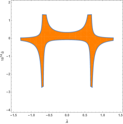
Figure 1: Constraints on $\tilde{\alpha}$ and $\tilde{A}$ from theoretical and observational bounds. The orange area is allowed by the constraints mentioned in the main text.

IV.2 $p_{m}=0$ , $\Lambda_{0}=0$

In this subsection, let us turn to consider the case where the theory has vanishing bare cosmological constant, namely, $p_{m}=0$ and $\Lambda_{0}=0$.

From (IV), it is straightforward to show that $\dot{H}(t)$ and $\rho_{m}$ are, respectively, given by

$$\dot{H}(t) = -\frac{3(1+\hat{\alpha}H^{2})H^{2}}{2(1+2\hat{\alpha}H^{2})},$$ (53)

$$\rho_{m} = 3H^{2}(1+\hat{\alpha}H^{2}).$$ (54)

Just like what we did in $\Lambda_{0}\neq 0$ case, four possible bounds on the model parameter $\tilde{\alpha}$ can be obtained (where, again, we have introduced a dimensionless parameter $\tilde{\alpha}=\hat{\alpha}H_{0}^{2}$).

• Constraints from $\beta_{1}$ and $\beta_{2}$

  In the present case, $\beta_{1}$ and $\beta_{2}$ become

  $$\beta_{1}=1+2\tilde{\alpha},$$ (55)

  $$\beta_{2}=1+2\tilde{\alpha}-6\tilde{\alpha}\cdot\frac{1+\tilde{\alpha}}{1+2\tilde{\alpha}}.$$ (56)

  The requirement that $\beta_{i}>0$ thus place a constraint on $\tilde{\alpha}$ as

  $$-0.5<\tilde{\alpha}<0.366025.$$ (57)

• Constraints from $w_{de}$

  The expression for $w_{de}$ now becomes

  $$w_{de}=\frac{1}{\tilde{\alpha}}\left(1-\frac{1+\tilde{\alpha}}{1+2\tilde{\alpha}}\right).$$ (58)

  The current bound on $w_{de}$ is $-1.1<w_{de}<-0.9$ Ade:2015xua implies that

  $$-1.0556<\tilde{\alpha}<-0.954545.$$ (59)

  Clearly, this result contradicts with (57), a theoretical requirement to guarantee the theory is free from ghost and instabilities. This strongly suggests that the model with vanishing bare cosmological constant is ruled out from current cosmological observations. In what follows, we will show another evidence to support this statement.

• Constraints from $\alpha_{M}$

  From (27) and (53) one gets

  $$\alpha_{M}=-\frac{6\tilde{\alpha}(1+\tilde{\alpha})}{(1+2\tilde{\alpha})^{2}}.$$ (60)

  Again we use the current cosmological constraints of $\alpha_{M}$, $-0.434<\alpha_{M}<0.945$ Noller:2018wyv , then we get

  $$-1.09311<\tilde{\alpha}<-0.89163,$$ (61)

  or

  $$-0.10837<\tilde{\alpha}<0.0931124.$$ (62)

  Clearly the bound (61) should be abandoned due to $\beta_{1},\beta_{2}>0$ .

• Constraints from the speed of GWs

  Using the bound on the speed of GWs Monitor:2017mdv ,

  $$-3\times 10^{-15}\leq c_{\rm gw}-1\leq 7\times 10^{-16},$$ (63)

  and the expression of $c^{2}_{\rm gw}$ of this case

  $$c^{2}_{\rm gw}=1-\frac{6\tilde{\alpha}(1+\tilde{\alpha})}{(1+2\tilde{\alpha})^{2}},$$ (64)

  we find the following bounds

  $$-1\times 10^{-15} \leq \tilde{\alpha}+1\leq 2\times 10^{-16},$$ (65)

  or

  $$-2.33\times 10^{-16} \leq \tilde{\alpha}\leq 1.0\times 10^{-15}.$$ (66)

  It is obvious that the bound (65) is not allowed because of (57).

In summary, if we put the inconsistency obtained from the constraint of $w_{de}$ aside, we naively have a stringent bound (66). However, we should be very careful here. If we take the current cosmological observations into consideration, we find there is an inconsistency in this case. Particularly, the current cosmological observations put a severe constraint on the ratio of energy densities between dark energy and matter (i.e. $\frac{\Omega_{de}}{\Omega_{m}}\sim\frac{7}{3}$). Direct computation shows that the present case leads to the following ratio

$$\frac{\Omega_{de}}{\Omega_{m}} = \frac{\rho_{GB}+0}{\rho_{m}}=\frac{3H_{0}^{2}-\rho_{m}}{\rho_{m}}$$ (67)

$$= -\frac{\tilde{\alpha}}{1+\tilde{\alpha}},$$

which is much much less than $7/3$ after combining the result (66). This provides another evidence, in addition to the one given in (57) and (59), for the inconsistency of the model with vanishing bare cosmological constant.

Including the integration constant $A$ in (14), there is same inconsistency obtained from the constraint of $w_{de}$. The region of the constraints from $\beta_{1},\beta_{2},$ and $w_{de}$ on $\tilde{\alpha}$ and $\tilde{A}$ have no intersection. Hence, we conclude that the model in question does not admit a cosmological solution with vanishing bare cosmological constant, $\Lambda_{0}=0$.

V The scalar perturbations

Now let us consider the scalar perturbations. We choose the unitary gauge, in which the fluctuation of the scalar field vanishes and all of the fluctuations are described by that of the spacetime metric. The line element is assumed as

$$\mathrm{d}s^{2}=-(1+2\Phi)\mathrm{d}t^{2}+2\partial_{i}\xi\mathrm{d}t\mathrm{d}x^{i}+a^{2}(1+2\Psi)\delta_{ij}\mathrm{d}x^{i}\mathrm{d}x^{j}.$$ (68)

Varying the action with respect to $\Phi$ and $\xi$ leads to two constraints, corresponding to the energy and momentum constraints,

$$\beta_{1}\dot{\Psi}+\gamma_{1}\Phi = 0,$$ (69)

$$\gamma_{1}\frac{\vec{\nabla}^{2}\xi}{a^{2}}-\beta_{1}\frac{\vec{\nabla}^{2}\Psi}{a^{2}}-3\gamma_{1}\dot{\Psi}+\gamma_{2}\Phi = 0.$$ (70)

Here we introduce two coefficients,

$$\gamma_{1}=6\hat{\alpha}H^{2}\dot{\phi}+6\hat{\alpha}H\dot{\phi}^{2}+2\hat{\alpha}\dot{\phi}^{3}-H,$$ (71)

$$\gamma_{2}=3H^{2}-2\Lambda_{0}.$$ (72)

The variation of $\Psi$ then gives a nontrivial field equation

$$-H\beta_{2}\vec{\nabla}^{2}\xi-\beta_{1}\vec{\nabla}^{2}\dot{\xi}+3a^{2}\beta_{1}\ddot{\Psi}-\beta_{2}\vec{\nabla}^{2}\Psi+\gamma_{3}\dot{\Psi}$$

$$-\beta_{1}\vec{\nabla}^{2}\Phi+3a^{2}\gamma_{1}\dot{\Phi}+\gamma_{4}\Phi=0,$$ (73)

where $\gamma_{3}$ and $\gamma_{4}$ are defined by

$$\gamma_{3}=3a\dot{a}(2\beta_{1}+\beta_{2}),$$ (74)

$$\gamma_{4}=3a^{2}(3H\gamma_{1}+\dot{\gamma}_{1}).$$ (75)

Using the two constraints we can eliminate $\Phi$ and $\xi$, and get the equation for $\Psi$,

$$\sigma_{1}\ddot{\Psi}+(3H\sigma_{1}+\dot{\sigma_{1}})\dot{\Psi}-\frac{\sigma_{2}}{a^{2}}\vec{\nabla}^{2}\Psi=0.$$ (76)

The corresponding quadratic action is

$$S_{\Psi}=\int\mathrm{d}t\mathrm{d}^{3}xa^{3}\left(\sigma_{1}\dot{\Psi}^{2}-\frac{\sigma_{2}}{a^{2}}\vec{\nabla}^{2}\Psi\right).$$ (77)

The coefficients $\sigma_{1}$ and $\sigma_{2}$ are defined as

$$\sigma_{1}=3\beta_{1}+\frac{\beta_{1}^{2}}{\gamma_{1}^{2}}\gamma_{2},$$ (78)

$$\sigma_{2}=-\beta_{2}\left(1+\frac{H\beta_{1}}{\gamma_{1}}\right)-\beta_{1}\frac{\mathrm{d}}{\mathrm{d}t}\left(\frac{\beta_{1}}{\gamma_{1}}\right).$$ (79)

Similar to the tensor modes, the coefficients $\sigma_{1}$ and $\sigma_{2}$ should be positive to avoid ghost and gradient instability. Let us follow the method in section IV.

$$\beta_{1} = 1-2\hat{\alpha}\left(H-\frac{A}{a}\right)^{2}+4\hat{\alpha}\left(H-\frac{A}{a}\right)H,$$

$$\beta_{2} = 1+2\hat{\alpha}\left(H-\frac{A}{a}\right)^{2}-4\hat{\alpha}\left(-\dot{H}-\frac{A}{a}H\right),$$

$$\gamma_{1} = -6\hat{\alpha}H^{2}\left(H-\frac{A}{a}\right)+6\hat{\alpha}H\left(H-\frac{A}{a}\right)^{2}$$

$$-2\hat{\alpha}\left(H-\frac{A}{a}\right)^{3}-H,$$

$$\gamma_{2} = -3H^{2}-4\dot{H}-2\hat{\alpha}\left(\frac{A}{a}\right)^{4}-2\hat{\alpha}H^{2}\left(3H^{2}+4\dot{H}\right),$$

with $\Lambda_{0}=3H^{2}+2\dot{H}+\hat{\alpha}\left(\frac{A}{a}\right)^{4}+3\hat{\alpha}H^{4}+4\hat{\alpha}H^{2}\dot{H}$.

At present, substituting (50) into (V), we have (IV.1) and

$$\gamma_{1} = \left(-6\tilde{\alpha}\left(1-\tilde{A}\right)+6\tilde{\alpha}\left(1-\tilde{A}\right)^{2}\right.$$

$$\left.-2\tilde{\alpha}\left(1-\tilde{A}\right)^{3}-1\right)H_{0},$$

$$\gamma_{2} = \frac{6}{5}\left(5\tilde{\alpha}\left(\tilde{A}^{4}-1\right)-1\right)H_{0}^{2}.$$ (81)

Using $\sigma_{1}>0$ and $\sigma_{2}>0$, we get the constraints on $\tilde{\alpha}$ and $\tilde{A}_{0}$ as shown in Fig 2.

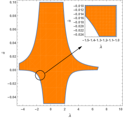
Figure 2: Constraints on $\tilde{\alpha}$ and $\tilde{A}$ from theoretical and observational bounds, the orange area satisfies $\sigma_{1}>0$ and $\sigma_{2}>0$. The zoomed-in region is to show that around $-1.5<\tilde{A}<-1$, the current constraint obtained by $\sigma_{1}>0$ and $\sigma_{2}>0$ is much looser ($12$ order of magnitude looser) than the one obtained from GW observations as shown in Fig. 1.

In order to see whether the above results will be effected by coupling a matter field, in what follows we will consider the case where matter field is mimicked by a k-essence field $\chi$ Kobayashi:2019hrl . Following what we did for the case without $\chi$, we show that the quadratic action, after fixing the gauge, can be reduced to the modes $\Psi$ and $\delta\chi$ solely DeFelice:2011bh ; Kobayashi:2019hrl

$$S^{(2)}_{M} = \int\mathrm{d}t\mathrm{d}^{3}xa^{3}[G_{ij}\dot{Q}_{i}\dot{Q}_{j}-\frac{1}{a^{2}}F_{ij}(\partial Q_{i})(\partial Q_{j})$$

$$-D_{ij}Q_{i}\dot{Q}_{j}-B_{ij}Q_{i}Q_{j}],$$

where

$$G_{ij} = \left(\begin{array}[]{cc}{\sigma_{1}}+Z&-Z\\ -Z&Z\end{array}\right),\quad F_{ij}=\left(\begin{array}[]{cc}{\sigma_{2}}&-c_{m}^{2}Z\\ -c_{m}^{2}Z&c_{m}^{2}Z\end{array}\right),$$ (87)

$$Q_{i} \equiv \left(\Psi,\frac{\beta_{1}}{\gamma_{1}}\frac{\delta\chi}{\dot{\chi}}\right),\quad Z\equiv\left(\frac{\beta_{1}}{\gamma_{1}}\right)^{2}\frac{\rho^{(\chi)}+p^{(\chi)}}{2c_{m}^{2}}.$$ (88)

Here $c_{m}^{2}\equiv\frac{\dot{\rho}^{(\chi)}}{\dot{p}^{(\chi)}}$ with $\rho^{(\chi)}+p^{(\chi)}>0$, and $\rho^{(\chi)}$ and $p^{(\chi)}$ are respectively energy density, pressure of the fluid mimicked by k-essence field $\chi$. $D_{ij},B_{ij}$ are the components of the 2 × 2 matrices DeFelice:2011bh . Avoiding ghost instabilities requires that $\sigma_{1}>0$ and $Z>0$. Due to det$(v^{2}G_{ij}-F_{ij})=0$, the stability conditions including an additional perfect fluid become $\sigma_{1}>0$ and $\sigma_{2}>\frac{1}{2}\left(\frac{\beta_{1}}{\gamma_{1}}\right)^{2}(\rho^{(\chi)}+p^{(\chi)})>0$, in which $v$ is the propagation speeds of the two scalar modes. In summary, compared to the case without matter, the stability conditions are changed to $\sigma_{1}>0$ and $\sigma_{2}>\frac{1}{2}\left(\frac{\beta_{1}}{\gamma_{1}}\right)^{2}(\rho^{(\chi)}+p^{(\chi)})>0$, which depends on the values of $\rho^{(\chi)}$ and $p^{(\chi)}$. As an example, suppose that $\chi$ represents dark matter. Let us use the Plank 2015 data Aghanim:2018eyx , where dark matter density parameter and radiation density parameter are $\Omega_{c}=0.2589±0.0057,$ $\Omega_{R}=0$. Then the constraints on $\tilde{\alpha}$ and $\tilde{A}$ can be obtained as shown in Fig 3.

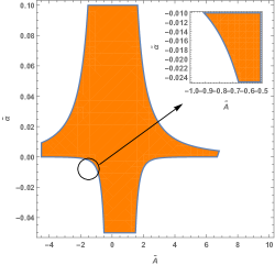
Figure 3: For simplicity we set $\Omega_{c}=0.2589$. Then constraints on $\tilde{\alpha}$ and $\tilde{A}$ from theoretical and observational bounds, the orange area satisfies $\sigma_{1}>0$ and $\sigma_{2}>\frac{1}{2}\left(\frac{\beta_{1}}{\gamma_{1}}\right)^{2}(\rho^{(\chi)}+p^{(\chi)})>0$. The zoomed-in region is to show that around $-1.0<\tilde{A}<-0.5$.

It is clear that the constraints on $\tilde{\alpha}$ and $\tilde{A}$ are stricter by comparing with Fig 2. For the case that $\chi$ represents radiation, however, the enhancement of the constraints is negligible due to the ignorable radiation density. As a result, for this case we have almost the same constraints as those for the pure gravity case, i.e, the one without coupling matter field.

VI Conclusions and Discussions

In this paper, we give detailed analysis about the theoretical and observational constraints on the regularized 4D EGB theory. Our analysis is based on linear perturbation around the FRW universe and is limited to the tensor modes such that we can deal with the gravitational waves. For these modes, the fluctuations of the scalar field $\phi$ are decoupled, and a set of linear perturbation equations are obtained, through which the speed of GWs can be read off.

Our results can be divided into two classes according to whether the bare cosmological constant $\Lambda_{0}$ is vanishing or not. For $\Lambda_{0}=0$, we find that theoretical requirements of the model are contradicted with the current observational results, indicating that the theory of this case should be ruled out. We make the conclusion from two strong evidences: one is from the theoretical contradiction with the current observations of $w_{de}$, the other comes from the huge (about 15 orders of magnitude) deviations between constraints from GW170817 and GRB 170817A and constraints from the current cosmological constraint on the ratio of energy densities between dark energy and matter, $\frac{\Omega_{de}}{\Omega_{m}}$. Including the integration constant $A$ in (14) does not remove the inconsistency obtained from the constraint of $w_{de}$ on $\tilde{\alpha}$ and $\tilde{A}$.

For $\Lambda_{0}\neq 0$, however, one can place a stringent constraint on the dimensionless model parameter $\tilde{\alpha}$ (and $\Lambda_{0}$, since $\Lambda_{0}$ and $\tilde{\alpha}$ are not independent in this case as shown in (49)). Compared to theoretical and cosmological constraints (values of $w_{de}$ and $\alpha_{M}$), the constraint from the speed of GWs measured by GW170817 and GRB 170817A is much more stringent. Specifically, it is given by $-7.78\times 10^{-16}\leq\tilde{\alpha}\leq 3.33\times 10^{-15}$. In should be noted that in a modified version of the theory Aoki:2020iwm , if the additional modification – $k^{4}$ term of the dispersion relation is ignored, the model is effectively compatible with our model, and the speed of GWs place an upper bound $\alpha<10^{50}eV^{-2}$, which is equivalent to $\tilde{\alpha}<10^{-16}$ in the our notation and is consistent with our result. In contrast, if the $k^{4}$ term is taken into considerations, the modified version of the theory Aoki:2020iwm gives much stricter constraints. As $A$ is taken into consideration, we find that for $|\tilde{A}|\lesssim 1.35$ we have constraints $|\tilde{\alpha}|<3\times 10^{-14}$. In addition, the case with $|\tilde{A}|\gtrsim 1.35$ is excluded by observational data as shown in Fig. 1.

Scalar perturbations in the universe dominated by $\phi$ has been considered in section V. The Fig. 2 shows that the current constraint obtained by $\sigma_{1}>0$ and $\sigma_{2}>0$ is much looser ($12$ order of magnitude looser) than the one obtained by GW observations as shown in Fig. 1. While including the other kind of matter, the stability conditions are changed to $\sigma_{1}>0$ and $\sigma_{2}>\frac{1}{2}\left(\frac{\beta_{1}}{\gamma_{1}}\right)^{2}(\rho^{(\chi)}+p^{(\chi)})>0$, which depends on the values of $\rho^{(\chi)}$ and $p^{(\chi)}$. If $\chi$ represents dark matter, then the constraint on $\tilde{\alpha}$ and $\tilde{A}$ will be stricter as shown in Fig 3.

Note added: After this work was completed, we learned a similar work 1803359 , which appeared in arXiv a few days before. Their work focused on $A=0$ case (where $A=0$ corresponds to $C=0$ in the notation of 1803359 ). Besides, it is worth noting that much stronger constraints in 1803359 have been obtained from other sources. For example, $-10^{10}m^{2}\lesssim\alpha\lesssim 10^{8}m^{2}$ from BH binary inspiral, $\alpha\simeq 10^{10}m^{2}$ from LAGEOS satellites and so on.

References

- (1) B. P. Abbott et al. (LIGO Scientific Collaboration Virgo Collaboration), “Observation of Gravitational Waves from a Binary Black Hole Merger,” Phys. Rev. Lett. 116, 061102 (2016).
- (2) B. P. Abbott et al. (LIGO Scientific Collaboration Virgo Collaboration), “GW170817: Observation of Gravitational Waves from a Binary Neutron Star Inspiral,” Phys. Rev. Lett. 119, no.16, 161101 (2017).
- (3) A. Goldstein, P. Veres, E. Burns, M. Briggs, R. Hamburg, D. Kocevski, C. Wilson-Hodge, R. Preece, S. Poolakkil, O. Roberts, C. Hui, V. Connaughton, J. Racusin, A. von Kienlin, T. Dal Canton, N. Christensen, T. Littenberg, K. Siellez, L. Blackburn, J. Broida, E. Bissaldi, W. Cleveland, M. Gibby, M. Giles, R. Kippen, S. McBreen, J. McEnery, C. Meegan, W. Paciesas and M. Stanbro, “An Ordinary Short Gamma-Ray Burst with Extraordinary Implications: Fermi-GBM Detection of GRB 170817A,” Astrophys. J. Lett. 848, no.2, L14 (2017).
- (4) V. Savchenko, C. Ferrigno, E. Kuulkers, A. Bazzano, E. Bozzo, S. Brandt, J. Chenevez, T. L. Courvoisier, R. Diehl, A. Domingo, L. Hanlon, E. Jourdain, A. von Kienlin, P. Laurent, F. Lebrun, A. Lutovinov, A. Martin-Carrillo, S. Mereghetti, L. Natalucci, J. Rodi, J. P. Roques, R. Sunyaev and P. Ubertini, “INTEGRAL Detection of the First Prompt Gamma-Ray Signal Coincident with the Gravitational-wave Event GW170817,” Astrophys. J. Lett. 848, no.2, L15 (2017).
- (5) B. P. Abbott et al. (LIGO Scientific Collaboration Virgo Collaboration), “Gravitational Waves and Gamma-rays from a Binary Neutron Star Merger: GW170817 and GRB 170817A,” Astrophys. J. Lett. 848, no.2, L13 (2017).
- (6) B. P. Abbott et al. (LIGO Scientific Collaboration Virgo Collaboration), “GW151226: Observation of Gravitational Waves from a 22-Solar-Mass Binary Black Hole Coalescence,” Phys. Rev. Lett. 116, no.24, 241103 (2016).
- (7) B. P. Abbott et al. (LIGO Scientific Collaboration Virgo Collaboration), “GW170104: Observation of a 50-Solar-Mass Binary Black Hole Coalescence at Redshift 0.2,” Phys. Rev. Lett. 118, no.22, 221101 (2017).
- (8) B. P. Abbott et al. (LIGO Scientific Collaboration Virgo Collaboration), “GW170608: Observation of a 19-solar-mass Binary Black Hole Coalescence,” Astrophys. J. 851, no.2, L35 (2017).
- (9) B. P. Abbott et al. (LIGO Scientific Collaboration Virgo Collaboration), “GW170814: A Three-Detector Observation of Gravitational Waves from a Binary Black Hole Coalescence,” Phys. Rev. Lett. 119, no.14, 141101 (2017).
- (10) G. W. Horndeski, “Second-order scalar-tensor field equations in a four-dimensional space,” Int. J. Theor. Phys. 10, 363-384 (1974).
- (11) Y. Fujii, K. Maeda, “The scalar-tensor theory of gravitation,” (Cambridge University Press, 2007).
- (12) N. Chow and J. Khoury, “Galileon Cosmology,” Phys. Rev. D 80, 024037 (2009).
- (13) S. Tsujikawa, “Modified gravity models of dark energy,” Lect. Notes Phys. 800, 99-145 (2010).
- (14) S. H. Chen, J. B. Dent, S. Dutta and E. N. Saridakis, “Cosmological perturbations in f(T) gravity,” Phys. Rev. D 83, 023508 (2011).
- (15) T. Clifton, P. G. Ferreira, A. Padilla and C. Skordis, “Modified Gravity and Cosmology,” Phys. Rept. 513, 1-189 (2012).
- (16) J. Gleyzes, D. Langlois, F. Piazza and F. Vernizzi, “Exploring gravitational theories beyond Horndeski,” JCAP 02, 018 (2015).
- (17) M. Crisostomi, K. Koyama and G. Tasinato, “Extended Scalar-Tensor Theories of Gravity,” JCAP 04, 044 (2016).
- (18) J. Sakstein and B. Jain, “Implications of the Neutron Star Merger GW170817 for Cosmological Scalar-Tensor Theories,” Phys. Rev. Lett. 119, no.25, 251303 (2017).
- (19) J. M. Ezquiaga and M. Zumalacárregui, “Dark Energy After GW170817: Dead Ends and the Road Ahead,” Phys. Rev. Lett. 119, no.25, 251304 (2017).
- (20) M. Green, J. Moffat and V. Toth, “Modified Gravity (MOG), the speed of gravitational radiation and the event GW170817/GRB 170817A,” Phys. Lett. B 780, 300-302 (2018).
- (21) A. Casalino, M. Rinaldi, L. Sebastiani and S. Vagnozzi, “Alive and well: mimetic gravity and a higher-order extension in light of GW170817,” Class. Quant. Grav. 36, no.1, 017001 (2019).
- (22) T. Baker, E. Bellini, P. Ferreira, M. Lagos, J. Noller and I. Sawicki, “Strong constraints on cosmological gravity from GW170817 and GRB 170817A,” Phys. Rev. Lett. 119, no.25, 251301 (2017).
- (23) S. Mirshekari, N. Yunes and C. M. Will, “Constraining Generic Lorentz Violation and the Speed of the Graviton with Gravitational Waves,” Phys. Rev. D 85, 024041 (2012).
- (24) J. Beltran Jimenez, F. Piazza and H. Velten, “Evading the Vainshtein Mechanism with Anomalous Gravitational Wave Speed: Constraints on Modified Gravity from Binary Pulsars,” Phys. Rev. Lett. 116, no.6, 061101 (2016).
- (25) P. M. Chesler and A. Loeb, “Constraining Relativistic Generalizations of Modified Newtonian Dynamics with Gravitational Waves,” Phys. Rev. Lett. 119, no.3, 031102 (2017).
- (26) P. Creminelli and F. Vernizzi, “Dark Energy after GW170817 and GRB 170817A,” Phys. Rev. Lett. 119, no.25, 251302 (2017).
- (27) A. Nishizawa, “Generalized framework for testing gravity with gravitational-wave propagation. I. Formulation,” Phys. Rev. D 97, no.10, 104037 (2018).
- (28) S. Arai and A. Nishizawa, “Generalized framework for testing gravity with gravitational-wave propagation. II. Constraints on Horndeski theory,” Phys. Rev. D 97, no.10, 104038 (2018).
- (29) R. A. Battye, F. Pace and D. Trinh, “Gravitational wave constraints on dark sector models,” Phys. Rev. D 98, no.2, 023504 (2018).
- (30) K. Stelle, “Renormalization of Higher Derivative Quantum Gravity,” Phys. Rev. D 16, 953-969 (1977).
- (31) D. Lovelock, “The Einstein tensor and its generalizations,” J. Math. Phys. 12, 498-501 (1971).
- (32) B. Zumino, “Gravity Theories in More Than Four-Dimensions,” Phys. Rept. 137, 109 (1986).
- (33) D. Glavan and C. Lin, “Einstein-Gauss-Bonnet Gravity in Four-Dimensional Spacetime,” Phys. Rev. Lett. 124, no.8, 081301 (2020).
- (34) S. Nojiri and S. D. Odintsov, “Novel cosmological and black hole solutions in Einstein and higher-derivative gravity in two dimensions,” EPL 130, no.1, 10004 (2020).
- (35) R. A. Konoplya and A. F. Zinhailo, “Quasinormal modes, stability and shadows of a black hole in the 4D Einstein–Gauss–Bonnet gravity,” Eur. Phys. J. C 80, no.11, 1049 (2020).
- (36) M. Guo and P. C. Li, “Innermost stable circular orbit and shadow of the Einstein–Gauss–Bonnet black hole,” Eur. Phys. J. C 80, no.6, 588 (2020).
- (37) P. G. S. Fernandes, “Charged Black Holes in AdS Spaces in Einstein Gauss-Bonnet Gravity,” Phys. Lett. B 805, 135468 (2020).
- (38) A. Casalino, A. Colleaux, M. Rinaldi and S. Vicentini, “Regularized Lovelock gravity,” [arXiv:2003.07068 [gr-qc]].
- (39) R. Konoplya and A. Zhidenko, “Black holes in the four-dimensional Einstein-Lovelock gravity,” Phys. Rev. D 101, no.8, 084038 (2020).
- (40) K. Hegde, A. Naveena Kumara, C. A. Rizwan, A. K. M. and M. S. Ali, “Thermodynamics, Phase Transition and Joule Thomson Expansion of novel 4-D Gauss Bonnet AdS Black Hole,” [arXiv:2003.08778 [gr-qc]].
- (41) S. G. Ghosh and S. D. Maharaj, “Radiating black holes in the novel 4D Einstein–Gauss–Bonnet gravity,” Phys. Dark Univ. 30, 100687 (2020).
- (42) D. D. Doneva and S. S. Yazadjiev, “Relativistic stars in 4D Einstein-Gauss-Bonnet gravity,” [arXiv:2003.10284 [gr-qc]].
- (43) Y. P. Zhang, S. W. Wei and Y. X. Liu, “Spinning Test Particle in Four-Dimensional Einstein–Gauss–Bonnet Black Holes,” Universe 6, no.8, 103 (2020).
- (44) R. A. Konoplya and A. Zhidenko, “BTZ black holes with higher curvature corrections in the 3D Einstein-Lovelock gravity,” Phys. Rev. D 102, no.6, 064004 (2020).
- (45) D. V. Singh and S. Siwach, “Thermodynamics and P-v criticality of Bardeen-AdS Black Hole in 4 Einstein-Gauss-Bonnet Gravity,” Phys. Lett. B 808, 135658 (2020).
- (46) S. G. Ghosh and R. Kumar, “Generating black holes in Einstein-Gauss-Bonnet gravity,” Class. Quant. Grav. 37, no.24, 245008 (2020).
- (47) R. A. Konoplya and A. Zhidenko, “(In)stability of black holes in the Einstein–Gauss–Bonnet and Einstein–Lovelock gravities,” Phys. Dark Univ. 30, 100697 (2020).
- (48) A. Kumar and R. Kumar, “Bardeen black holes in the novel Einstein-Gauss-Bonnet gravity,” [arXiv:2003.13104 [gr-qc]].
- (49) C. Y. Zhang, P. C. Li and M. Guo, “Greybody factor and power spectra of the Hawking radiation in the Einstein–Gauss–Bonnet de-Sitter gravity,” Eur. Phys. J. C 80, no.9, 874 (2020).
- (50) S. A. Hosseini Mansoori, “Thermodynamic geometry of the novel 4-D Gauss Bonnet AdS Black Hole,” [arXiv:2003.13382 [gr-qc]].
- (51) S. W. Wei and Y. X. Liu, “Extended thermodynamics and microstructures of four-dimensional charged Gauss-Bonnet black hole in AdS space,” Phys. Rev. D 101, no.10, 104018 (2020).
- (52) D. V. Singh, S. G. Ghosh and S. D. Maharaj, “Clouds of strings in 4 Einstein–Gauss–Bonnet black holes,” Phys. Dark Univ. 30, 100730 (2020).
- (53) M. S. Churilova, “Quasinormal modes of the Dirac field in the consistent 4D Einstein–Gauss–Bonnet gravity,” Phys. Dark Univ. 31, 100748 (2021).
- (54) S. U. Islam, R. Kumar and S. G. Ghosh, “Gravitational lensing by black holes in the Einstein-Gauss-Bonnet gravity,” JCAP 09, 030 (2020).
- (55) A. K. Mishra, “Quasinormal modes and strong cosmic censorship in the regularised 4D Einstein–Gauss–Bonnet gravity,” Gen. Rel. Grav. 52, no.11, 106 (2020).
- (56) A. Kumar and S. G. Ghosh, “Hayward black holes in the novel Einstein-Gauss-Bonnet gravity,” [arXiv:2004.01131 [gr-qc]].
- (57) C. Liu, T. Zhu and Q. Wu, “Thin Accretion Disk around a four-dimensional Einstein-Gauss-Bonnet Black Hole,” Chin. Phys. C 45, 015105 (2021).
- (58) S.-L. Li, P. Wu, and H. Yu, “Stability of the Einstein Static Universe in 4D Gauss-Bonnet Gravity,” [arXiv:2004.02080 [gr-qc]].
- (59) R. A. Konoplya and A. F. Zinhailo, “Grey-body factors and Hawking radiation of black holes in Einstein-Gauss-Bonnet gravity,” Phys. Lett. B 810, 135793 (2020).
- (60) M. Heydari-Fard, M. Heydari-Fard and H. Sepangi, “Bending of light in novel 4 Gauss-Bonnet-de Sitter black holes by Rindler-Ishak method,” [arXiv:2004.02140 [gr-qc]].
- (61) X. H. Jin, Y. X. Gao and D. J. Liu, “Strong gravitational lensing of a 4-dimensional Einstein–Gauss–Bonnet black hole in homogeneous plasma,” Int. J. Mod. Phys. D 29, no.09, 2050065 (2020).
- (62) C. Y. Zhang, S. J. Zhang, P. C. Li and M. Guo, “Superradiance and stability of the regularized 4D charged Einstein-Gauss-Bonnet black hole,” JHEP 08, 105 (2020).
- (63) B. Eslam Panah, K. Jafarzade and S. H. Hendi, “Charged 4D Einstein-Gauss-Bonnet-AdS Black Holes: Shadow, Energy Emission, Deflection Angle and Heat Engine,” Nucl. Phys. B 961, 115269 (2020).
- (64) A. Aragón, R. Bécar, P. A. González and Y. Vásquez, “Perturbative and nonperturbative quasinormal modes of 4D Einstein–Gauss–Bonnet black holes,” Eur. Phys. J. C 80, no.8, 773 (2020).
- (65) S. J. Yang, J. J. Wan, J. Chen, J. Yang and Y. Q. Wang, “Weak cosmic censorship conjecture for the novel charged Einstein-Gauss-Bonnet black hole with test scalar field and particle,” Eur. Phys. J. C 80, no.10, 937 (2020).
- (66) Z. C. Lin, K. Yang, S. W. Wei, Y. Q. Wang and Y. X. Liu, “Equivalence of solutions between the four-dimensional novel and regularized EGB theories in a cylindrically symmetric spacetime,” Eur. Phys. J. C 80, no.11, 1033 (2020).
- (67) K. Yang, B. M. Gu, S. W. Wei and Y. X. Liu, “Born–Infeld black holes in 4D Einstein–Gauss–Bonnet gravity,” Eur. Phys. J. C 80, no.7, 662 (2020).
- (68) G. Narain and H. Q. Zhang, “Cosmic evolution in novel-Gauss Bonnet Gravity,” [arXiv:2005.05183 [gr-qc]].
- (69) G. Narain and H. Q. Zhang, “Lorentzian quantum cosmology in novel Gauss-Bonnet gravity from Picard-Lefschetz methods,” [arXiv:2006.02298 [gr-qc]].
- (70) X. H. Ge and S. J. Sin, “Causality of black holes in 4-dimensional Einstein–Gauss–Bonnet–Maxwell theory,” Eur. Phys. J. C 80, no.8, 695 (2020).
- (71) A. Banerjee, T. Tangphati, D. Samart and P. Channuie, “Quark Stars in 4D Einstein-Gauss-Bonnet gravity with an Interacting Quark Equation of State,” [arXiv:2007.04121 [gr-qc]].
- (72) W. Y. Ai, “A note on the novel 4D Einstein–Gauss–Bonnet gravity,” Commun. Theor. Phys. 72, no.9, 095402 (2020).
- (73) M. Gürses, T. Ç. Şişman and B. Tekin, “Is there a novel Einstein–Gauss–Bonnet theory in four dimensions?,” Eur. Phys. J. C 80, no.7, 647 (2020).
- (74) H. Lu and Y. Pang, “Horndeski gravity as limit of Gauss-Bonnet,” Phys. Lett. B 809, 135717 (2020).
- (75) T. Kobayashi, “Effective scalar-tensor description of regularized Lovelock gravity in four dimensions,” JCAP 07, 013 (2020).
- (76) R. A. Hennigar, D. Kubizňák, R. B. Mann and C. Pollack, “On taking the D 4 limit of Gauss-Bonnet gravity: theory and solutions,” JHEP 07, 027 (2020).
- (77) P. G. S. Fernandes, P. Carrilho, T. Clifton and D. J. Mulryne, “Derivation of Regularized Field Equations for the Einstein-Gauss-Bonnet Theory in Four Dimensions,” Phys. Rev. D 102, no.2, 024025 (2020).
- (78) S. Mahapatra, “A note on the total action of 4D Gauss–Bonnet theory,” Eur. Phys. J. C 80, no.10, 992 (2020).
- (79) F. W. Shu, “Vacua in novel 4D Einstein-Gauss-Bonnet Gravity: pathology and instability?,” Phys. Lett. B 811, 135907 (2020).
- (80) K. Aoki, M. A. Gorji and S. Mukohyama, “Cosmology and gravitational waves in consistent Einstein-Gauss-Bonnet gravity,” JCAP 09, 014 (2020).
- (81) K. Van Acoleyen and J. Van Doorsselaere, “Galileons from Lovelock actions,” Phys. Rev. D 83, 084025 (2011).
- (82) S. M. Carroll, “Spacetime and Geometry”.
- (83) R. A. Konoplya and A. Zhidenko, “4 Einstein-Lovelock black holes: Hierarchy of orders in curvature,” Phys. Lett. B 807, 135607 (2020).
- (84) T. Kobayashi, “Horndeski theory and beyond: a review,” Rept. Prog. Phys. 82, no.8, 086901 (2019).
- (85) J. Bonifacio, K. Hinterbichler and L. A. Johnson, “Amplitudes and 4D Gauss-Bonnet Theory,” Phys. Rev. D 102, no.2, 024029 (2020).
- (86) P. Ade et al. [Planck], “Planck 2015 results. XIII. Cosmological parameters,” Astron. Astrophys. 594, A13 (2016).
- (87) J. Noller and A. Nicola, “Cosmological parameter constraints for Horndeski scalar-tensor gravity,” Phys. Rev. D 99, no.10, 103502 (2019).
- (88) A. De Felice and S. Tsujikawa, “Conditions for the cosmological viability of the most general scalar-tensor theories and their applications to extended Galileon dark energy models,” JCAP 02, 007 (2012).
- (89) N. Aghanim et al. [Planck], “Planck 2018 results. VI. Cosmological parameters,” Astron. Astrophys. 641, A6 (2020).
- (90) T. Clifton, P. Carrilho, P. G. S. Fernandes and D. J. Mulryne, “Observational Constraints on the Regularized 4D Einstein-Gauss-Bonnet Theory of Gravity,” Phys. Rev. D 102, no.8, 084005 (2020).