Pay Transparency and Gender Equality

Abstract

Since 2018 UK firms with at least 250 employees have been mandated to publicly disclose gender equality indicators. Exploiting variations in this mandate across firm size and time we show that pay transparency closes 18 percent of the gender pay gap by reducing men’s wage growth. The public availability of the equality indicators seems to influence employers’ response as worse performing firms and industries more exposed to public scrutiny reduce their gender pay gap the most. Employers are also 9 percent more likely to post wages in job vacancies, potentially in an effort to improve gender equality at entry level.

JEL codes: J08, J16, J24.
Keywords: pay transparency; gender equality; public disclosure.

1 Introduction

In recent years, many governments have adopted pay transparency policies with the aim of improving gender equality. By increasing the salience of gender gaps in the labor market, transparency measures are meant to act as an information shock that may alter the relative bargaining power of male and female employees vis-à-vis the firm. Coupled with the potential negative effects of unequal pay on firms’ reputation, transparency policies have the potential to improve women’s relative pay and career outcomes. The magnitude of these effects is also likely to depend on how strong and salient the information shock is.

This paper studies the impact of pay transparency in a context where firms’ gender equality performance is publicly disclosed. Each year since 2018, UK firms with at least 250 employees have been required to publish a series of gender equality indicators both on their own websites and on a dedicated government website. These indicators include percentage gaps in mean and median hourly pay, and the percentage of women in each quartile of the firm’s wage distribution.

We begin our analysis by studying the impact of this policy on the gender gap in hourly pay using the Annual Survey of Hours and Earnings (ASHE), the UK matched employer-employee data set, from 2013 to 2019. To identify causal effects, we exploit the variation across firm size and time in the application of the transparency policy. To avoid capturing any potential impact of this policy on firm size, we define the treatment status based on firms’ number of employees prior to the introduction of the mandate. To enhance comparability between the treatment and control groups, we restrict the sample to firms with +/-50 employees from the 250-employee threshold in our main specification.

Our results show that the UK pay transparency policy leads to an 18 percent reduction in the gender pay gap, off a base of £2.60. Importantly, and consistent with the hypothesis that pay transparency reduces the relative bargaining power of better-paid employees (Cullen and Pakzad-Hurson 2021), we find that this effect is driven by a significant 2.6 percent decrease in men’s real hourly pay in treated firms relative to control ones. Further evidence suggests that this slowdown of men’s pay growth is the result of fewer promotions accompanied by nominal cuts in highly paid occupations.

Event-study exercises show that these results are not driven by different pre-policy trends in the outcomes of interest between treatment and control groups. A battery of placebo regressions further exclude the possibility that our estimates capture the impact of time shocks affecting firms above and below the 250-employee threshold differently. Also, our estimates are not sensitive to choices made in the main specification, such as the bandwidth around the 250-employee cutoff.

As for the mechanisms behind these results, we provide several pieces of evidence that point to the importance of the public availability of the equality indicators to increase firms’ accountability. First, we find descriptive evidence for a behavioural response whereby worse performing firms in 2018 – employers reporting a larger gender pay gap in 2018 – decrease their gender pay gap the most between 2018 and 2019. Second, we use two YouGov surveys that, since 2018, measure firms’ reputation using representative samples of, respectively, British women and British employees, to show that, each year, firms publishing a larger gender pay gap obtain worse placements in both the Women’s Rankings and the Workforce Rankings. Third, we show that the drop in men’s real pay is larger in the two sectors, “Distribution and Hospitality” and “Banking and Finance”, that are potentially the most exposed to public scrutiny, as measured by their presence in the YouGov surveys. In sum, by enhancing public scrutiny and enabling comparisons across firms, the public disclosure of the equality indicators may have magnified the disciplinary effects of the policy (Perez-Truglia and Troiano 2015, Luca 2018, Johnson 2020).

To complement these results, we study whether and how the policy affects firms’ hiring practices by combining the difference-in-differences strategy with a text analysis of online job vacancies collected by Burning Glass Technologies (BGT hereafter). One of the most remarkable findings of our analysis is that the policy does not directly improve women’s pay or career outcomes, despite this being an explicit goal of the legislation. One possibility is that it simply takes time for these improvements to materialize, while the policy could have the more immediate effect of increasing firms’ efforts to improve gender equality at the entry level. A growing number of papers document that a factor contributing to the persistence of the gender pay gap is the so-called gender ask gap, whereby women shy away from wage bargaining or propose a lower ask salary when stating how much they want to make in their next job (Babcock et al. 2003, Hall and Krueger 2012, Leibbrandt and List 2015, Card et al. 2016, Roussille 2020, Biasi and Sarsons 2022). Upfront wage information in the recruitment process may help address this gap by reducing the room for wage bargaining. Consistent with this hypothesis, we first show that, while less than 50 percent of BGT listings provide salary details, firms that are more likely to post wage information in their vacancies also tend to have a larger percentage of women at the top of the firm wage distribution and a lower gender pay gap. More importantly, while these are only correlations, we bring causal evidence that, after the introduction of the policy, the probability that targeted firms post wages in their job ads increases by 9 percent compared to the control group. In other words, the policy induces employers to provide upfront wage information, potentially in an effort to improve gender equality at the entry level.

Our paper contributes to different strands of literature. To begin with, we make several contributions to the growing number of studies analyzing the impact of pay transparency on the gender pay gap and wage inequality more broadly (Card et al. 2012, Mas 2017, Breza et al. 2018, Cullen and Perez-Truglia 2018, Burn and Kettler 2019, Dube et al. 2019, Bennedsen et al. 2021, Cullen and Pakzad-Hurson 2021, Cullen and Perez-Truglia 2021, Baker et al. 2022, Gulyas et al. 2022). The closest studies to ours are Bennedsen et al. (2021), Baker et al. (2022), and Gulyas et al. (2022). Baker et al. (2022) study the effect on the gender pay gap of a Canadian law requiring public sector organizations to publish employees’ salaries above a certain pay threshold, while Bennedsen et al. (2021) and Gulyas et al. (2022) analyze the effect on the gender pay gap of, respectively, a 2006 Danish law and a 2011 Austrian law, mandating that private firms provide their employees with pay data by gender and occupation. Both Bennedsen et al. (2021) and Baker et al. (2022) find that transparency leads to pay compression by slowing down men’s wage growth. In contrast, Gulyas et al. (2022) find no impact on individuals’ wages or the gender pay gap, and suggest that the fact that, in Austria, the pay information is not disclosed publicly may contribute to explain these null results. Relative to these studies, the UK legislation has two unique features that could help improve our understanding of the effects of pay transparency. First, the information disclosed focuses on the gender pay gap rather than pay levels by gender. While in the latter case, workers could react both to cross-gender comparisons and to comparisons with their own gender, in the UK this second channel is shut down. Second, in the UK setting, the information is disclosed publicly rather than provided exclusively to employees’ representatives, which allows us to study the role of performance comparisons and enhanced public scrutiny in influencing firms’ responses to the policy.

Our paper also contributes to the increasing number of studies that use job advert data to analyze different dimensions of the labor market (Deming and Kahn 2018, Adams et al. 2020, Azar et al. 2020a, Azar et al. 2020b). Our analysis of firms’ wage posting decision specifically adds to the literature on the gender ask gap, by considering potential employers’ responses to address this gap (Roussille 2020, Flinn and Mullins 2021, Biasi and Sarsons 2022). Moreover, this analysis complements contemporary work on the impact of pay history inquiry bans on recruitment practices (Sran et al. 2020), by showing that the content of job vacancies is influenced by broader management practices, such as pay transparency.

The paper proceeds as follows. Section 2 describes the institutional setting and the UK transparency policy. Section 3 presents the identification strategy, data, and impact of the policy on the gender pay gap. Section 4 illustrates the robustness checks. Section 5 studies the role of the publicly availability of the gender equality indicators in influencing firms’ response. Section 6 presents results on firms’ hiring practices. Section 7 concludes.

2 Institutional setting

In 2015, the UK government launched a process of consultations with employers to enhance pay transparency. At that time, the average gender pay gap for all employees in the UK stood at 19.1 percent. Moreover, women made up only 34 percent of managers, directors, and senior officials (Government Equalities Office 2015). According to the government’s view, “greater transparency will encourage employers and employees to consider what more can be done to close any pay gaps. Moreover, employers with a positive story to tell will attract the best talent” (Government Equalities Office 2015).

In February 2017, this process resulted in the passing of the Equality Act 2010 (Gender Pay Gap Information) Regulations 2017. This mandate requires all firms registered in Great Britain that have at least 250 employees to publish gender equality indicators both on their own website and on a dedicated website managed by the Government Equalities Office (GEO hereafter). Also, organizations that are part of a group must report individually. In sum, around 10,500 firms are subject to this mandate each year, representing only 0.4 percent of all UK firms but accounting for 40 percent of employment and 48 percent of turnover (Business Structure Database). To the best of our knowledge, no other substantial law exclusively targeted firms in this size band when the transparency mandate was introduced.

The timing of the publication of the equality indicators works as follows. Each year, if a firm has at least 250 employees by April 5th (the end of the financial year in the UK), it has to calculate the gender equality indicators as of that date, and publish them by the end of the following financial year. Firms themselves must calculate their number of employees using guidelines provided by the government. Importantly, they have to adopt an extended definition of an employee that includes agency workers. Partners of firms are also included in the definition of an employee but should not be included in the calculation of the indicators. Finally, part-time workers have the same weight as full-time workers in the calculations.

The indicators that firms have to report include: the gender gap in the median (mean) hourly pay, expressed relative to men’s pay; the gender gap in the median (mean) bonus pay, expressed relative to men’s bonus pay; the proportion of male and female employees who receive any bonus pay; and the percentage of female employees in each quartile of a company’s wage distribution. Table 1 provides sample means of these indicators for 2017/18 and 2018/19. Note that in mid-March 2020 the transparency mandate was temporarily paused due to the Coronavirus outbreak, and firms were only asked to start publishing the equality indicators again in October 2021. Considering this, our main analysis focuses on the effects of the policy in the first two years since its introduction, though Appendix Table A1 shows that the results do not change when adding data for the financial years 2019/20 and 2020/21.

The first row of Table 1 shows that the gender gap in median pay is just below 12 percent in 2017/18, and increases slightly in the following year. The gap in mean pay is around 14 percent in 2017/18, and instead decreases a little the year after. Both gaps in median and mean bonuses tend to be smaller than pay gaps but it is worth noting from the large standard deviation that some firms mistakenly reported their level gap rather than a percentage, making it difficult to interpret these bonus gaps. The proportion of women receiving bonus pay is smaller than for men in each year, and both increase slightly in the second year. The gender ratio along the wage distribution is balanced at the bottom, but less than 40 percent of employees in the upper part of the wage distribution are women. Also, the proportion of women in each quartile of the wage distribution increases slightly over the two years.

Clearly, the magnitude of these raw firm-level indicators depends both on compositional and observable factors, such as gender differences in educational choices, occupation held and experience, and unobservable factors such as employers’ unconscious biases and subtle discrimination on the workplace (Azmat et al. 2020, Bertrand 2020). As they are, these aggregate measures do not allow to distinguish the importance of each underlying factor, and statistics broken down by occupation, or even better hierarchy position, would be more informative in this respect. Yet, the firm-level indicators may reflect a compromise between the government’s will to disclose these statistics publicly, and firms’ privacy concerns, and it is a matter of empirical analysis to understand how effective they are at pushing firms to tackle the underlying causes of gender inequality. From now on, we will refer to these data as the GEO data.

Three other features of this policy are important to understand the UK context. First, the policy does not impose sanctions on firms that do not improve their gender equality indicators over time. However, the Equality and Human Rights Commission, the enforcement body responsible for this regulation, can issue court orders and unlimited fines for firms that do not publish these indicators. As of 2020, all firms targeted by the law were deemed to have complied. Panel A of Figure 1 reports the distribution of submission dates for the first two years that the mandate was in place. While some firms do not meet the deadline, the majority publish their data in the last month before it. Note also that only 235 firms with fewer than 250 employees published gender equality indicators in 2018. These represent less than 0.1 percent of active UK firms with fewer than 250 employees in 2018 (Business Structure Database). This tiny percentage is consistent with the hypothesis that firms are reluctant to disclose information on employees’ pay if they are not forced to do so (Siniscalco et al. 2017). It is also important to take into account this figure when thinking about the potential general equilibrium effects of this policy.

Second, according to a survey conducted on behalf of GEO prior to the introduction of this policy, out of 855 private and non-profit firms with at least 150 employees, only one third of firms had ever computed their gender pay gap, and just 3 percent had made these figures publicly available. Moreover, up to 13 percent declared that staff were discouraged from talking about their pay with colleagues and 3 percent reported that their contracts included a clause on pay secrecy (Downing et al. 2015). These figures suggest that the transparency policy is likely to represent an information shock both inside and outside the firm.

Finally, this policy is salient. Not only are the figures publicly available via both a dedicated government website and companies’ own website, but they also receive extensive media attention each year when they are published (BBC *bbc2018, The Guardian *guardian2018, Financial Times *ft2018, Financial Times *ft2019), and firms are not spared from “naming and shaming” articles. Importantly, Panel B of Figure 1 shows that Google searches for the term “gender pay gap” spike around each year’s deadline, indicating that this policy attracts significant public interest. And while there is no direct evidence that employees of targeted firms consult the gender equality indicators, the law imposes companies to publish this information on their website “in a manner that is accessible to all its employees and to the public; and for a period of at least three years beginning with the date of publication”, which makes it unlikely that employees are completely unaware of it.

3 Impact on the gender pay gap

3.1 Identification strategy

Our primary goal is to identify the impact of the UK pay transparency policy on the gender gap in hourly pay and unpack this into the effect on women’s and men’s pay. For this, we exploit the variation in the implementation of the policy across firm size and over time, and compare the evolution of the outcomes of interest in firms whose size is slightly above (treatment group) or below (control) the 250-employee cutoff. As firm size can be endogenously determined, we define treatment status based on firm size in 2015, prior to the start of the consultation process to implement the mandate. Moreover, to enhance comparability between treatment and control group, we consider firms with $+/-50$ employees from the 250 threshold in the main specification. As both choices could be considered to be arbitrary, we show in the next section that our results are robust both to the use of a different year to define the treatment status and to changes in the bandwidth used to construct the estimation sample. Based on these choices, we estimate the following triple-differences regression model that aims to estimate the relative impact of the policy on men’s and women’s outcomes:

$$Y_{ijt} = \alpha_{ij}+\theta^{M}_{t}+\theta^{F}_{t}+\beta\;(TreatedFirm_{j}*Post_{t})$$ (1)

$$+\gamma\;(TreatedFirm_{j}*Post_{t}*Fem_{i})$$

$$+X_{ijt}^{\prime}\pi+u_{ijt},$$

where $i$ is an employee working in firm $j$, which has between 200 and 300 employees, in year $t$, running between 2013 and 2019, and $M$ and $F$ stand respectively for men and women. The outcome $Y_{ijt}$ is either a pay or career outcome, as defined in the next Section. As for the regressors, $\alpha_{ij}$ are individual-firm fixed effects that capture the impact of individual-firm-specific time-invariant characteristics such as the quality of the match between the employee and the employer; $\theta^{M}_{t}$ and $\theta^{F}_{t}$ are gender-year fixed effects that control for time shocks common to all firms but gender-specific such as the introduction of family-friendly policies; $Fem_{i}$ is a dummy variable that is equal to one if $i$ is a woman; $TreatedFirm_{j}$ is a dummy variable equal to one if a firm has at least 250 employees in 2015; $Post_{t}$ is a dummy variable equal to one from 2018 onward. Note that, in our data, we observe outcomes over fiscal years, which is also the time span over which firms have to publish equality indicators. Hence, for instance, 2018 refers to the fiscal year 2017/18 that starts in April 2017 and ends in March 2018. The vector $X_{ijt}$ includes time-varying individual and firm controls. In our main specification, we only include region-specific time shocks to control for shocks to the local labor market where the firm operates and the individual works, though we present robustness checks in Section 4 where we alternatively include industry-specific time shocks, or individual controls such as age and age squared. Standard errors are clustered at the firm level.

Our main coefficient of interest is $\gamma$ which, conditional on the validity of this identification strategy, should capture any deviation from a parallel evolution in the outcome’s gender gap between the treatment and the control group due to the introduction of the mandate. Put differently, $\gamma$ should identify the differential effect of the policy on women compared to men. Equally important are $\beta$ and $\beta+\gamma$, which identify, respectively, the effect of the policy on male and female employees. Thus, at the bottom of results’ tables we also report the p-value of the t-test on women’s effect.

The validity of our identification strategy depends on three assumptions. First, it has to satisfy the parallel-trend assumption, that is, prior to the introduction of the policy, the evolution of the outcomes of interest must be comparable in treated and control firms. Second, our estimates should not capture the effect of other time shocks that coincide with the introduction of pay transparency and affect firms on either side of the 250-employee cutoff differently. Third, the results should not depend on the size of the bandwidth considered around the policy cutoff, nor should they depend on the year chosen to define the treatment status.

To support the validity of the parallel-trend assumption and study the dynamic impact of the pay transparency policy, we will open the discussion of our main findings by illustrating the results of the following event-study exercise:

$$Y_{ijt} = \alpha_{ij}+\theta^{M}_{t}+\theta^{F}_{t}+X_{ijt}^{\prime}\pi$$ (2)

$$+\sum_{k=2013}^{2019}\beta{{}_{k}}(TreatedFirm_{j}*\bm{1}[t=k])$$

$$+\sum_{k=2013}^{2019}\gamma{{}_{k}}(Fem_{i}*TreatedFirm_{j}*\bm{1}[t=k])+\nu_{ijt},$$

where $\bm{1}[t=k]$ is an indicator variable that takes value 1 when $t=k$ and 0 otherwise. In what follows, we take 2017, the year prior to the introduction of pay transparency, as the reference year.

Next, in Section 4, we will provide evidence that the other two conditions necessary for the validity of the identification are also met.

3.2 Data

To study the impact of the policy on the gender pay gap, we use the Annual Survey of Hours and Earnings (ASHE). ASHE is an employer survey covering 1 percent of the UK workforce that is conducted every year and is designed to be representative of the employee population. The ASHE sample is drawn from National Insurance records for working individuals, and the selected workers’ employers are required by law to complete the survey. Specifically, ASHE asks employers to report data on gender, pay, hours, and tenure for the selected employees, using a snapshot in April each year. Information on age, occupation, and industrial classification is also available. Once workers enter the survey, they are followed even when changing employer, though individuals are not observed when unemployed or out of the labor force. In practice, ASHE is an unbalanced panel data set at the employee level.

The main limitation of ASHE is its small sample size and the fact that we do not observe all the employees of a firm, which does not allow us to compute a firm-level measure of the gender pay gap. However, this is the only data set available in the UK that provides both a large range of employees’ outcomes, including salary components, and information on the total number of employees in a firm and year, which allows us to define the treatment status in our identification strategy. From ASHE, we create the following variables:

Pay measures. Our main variable of interest is employees’ hourly pay, including bonuses but excluding overtime pay; we also separately consider the basic hourly pay and bonus payments, as well as weekly pay and hours worked. To study the impact of the policy on pay variables, we take log transformations, while for bonuses we use the inverse hyperbolic sine transformation to take into account the fact that 80 percent of workers do not receive these payments. All monetary values are deflated using the ONS’ 2015 CPI Index. To complement the analysis on pay outcomes, we also study the impact of the policy on employees’ promotion prospects. For this, we follow the ONS’ definition of a promotion and construct a dummy variable that is equal to one if, within the same firm, an employee has experienced at least a 30 percent increase in his/her hourly pay since the previous year, and/or has acquired managerial responsibility since then (ONS *ONS2020promotions).

Career outcomes. To get a full understanding of the impact of the policy on employees, in our analysis we also consider its effects on job mobility. First, we use months of tenure in a firm to study mobility into that firm; this variable is missing for around 2 percent of the estimation sample. Second, we construct a dummy variable that is equal to one if the employee leaves the firm in $t+1$, either by moving to a different firm, or by leaving the labor market. Finally, we construct a dummy variable equal to one if a worker is employed in a managerial occupation (1-digit SOC 1).

In the main specification, we use data over the period 2013–2019. We start from 2013, as we can observe all outcomes since then, and stop in 2019, as we prefer not to include years affected by the pandemic. However, note that we use information from 2012 and 2020 to construct, respectively, the promotion dummy and the indicator for leaving a firm in $t+1$. In terms of sample restrictions, we drop individuals with missing id or missing firm id (0.5 percent of the sample); we drop secondary jobs (3 percent); we drop individuals who work at least once more than 100 hours per week and those with an hourly pay greater or equal to £1000 (0.2 percent). Our resulting sample is formed of 5,135 men and 4,451 women, for a total of 15,769 individual-year observations for men and 13,457 for women. We observe men across 2,929 firms and women across 2,640 firms.

Table 2 provides summary statistics for the main outcomes measured in the pre-policy period, 2013–2017. Several features are worth noting. First, the profile of workers in treated and control firms is remarkably similar. Second, focusing on the treatment group (columns 1 and 3), the unconditional gap in hourly pay amounts to £2.57, or 16 percent of men’s pay. This gap reaches 29 percent when looking at weekly pay, as there is also a 16 percent gap in hours worked. As for bonuses, there is a large gender gap in the probability of receiving bonuses (34 percent), and a very large gap in the amount received (61 percent). And while there is a 33 percent promotion gap in favor of women, there is a 30 percent gender gap in favor of men in the probability of working in managerial occupations. This drops to 5 percent if we consider technical, professional, and managerial occupations, that is the three highest-paid occupations based on the pre-policy median hourly pay at 1-digit SOC level. Men are also more likely to stay longer in a firm than women, and to work in the private sector – though this share is already around 80 percent for women, which prevents us from studying heterogeneous effects between public and private-sector employees. Finally, note that among both men and women, only one third of workers are covered by a collective agreement, which similarly limits our ability to study heterogeneous effects between unionized and non-unionized workers.

3.3 Results

This section presents the impact of the pay transparency policy on employees’ outcomes. Figure 2 shows the event studies for the gender gap in hourly pay, in Panel A, and the log hourly pay, separately for men and women, in Panels B and C. From these figures, we observe, first, that the evolution of the outcomes in the pre-policy period seems to be comparable across treatment and control groups, both for what concerns the gender pay gap, and separately for male and female employees’ pay. Second, Panel A shows that women’s pay increases relatively to men’s pay after the introduction of the policy, with this effect being significant at 10 percent in 2019. Third, from Panel B, we see that this dynamic is driven by a decrease in men’s hourly pay in treated firms relative to control firms after the introduction of the mandate, with this effect becoming significant at the 5 percent level in 2019. In contrast, the policy does not appear to have any visible impact on women’s pay (Panel C).

Table 3 reports the estimates of the corresponding average effects of the policy. Each column shows a different outcome. At the bottom of the table, we report the p-value of the t-test on the effect on women and the pre-policy mean for the treatment group calculated over the period 2013–2017. Consistent with the dynamics seen in the event studies, Column 1 shows that the policy leads to a significant 2.9 percentage-point increase in women’s hourly pay compared to men’s pay. Relative to the pre-policy value of 16 percent, this corresponds to an 18 percent decrease in the gender gap in hourly pay. Importantly, the coefficient on TreatedFirm*Post confirms that this effect is driven by a 2.6 percent significant reduction in men’s real hourly pay, while on average, the policy has no impact on women’s pay.

While these results are consistent with the estimated effects of pay transparency in other settings (Bennedsen et al. 2021, Baker et al. 2022), they definitely deserve further explanations. On the one hand, we need to explain whether the fall in men’s real hourly pay is driven by bonuses’ cuts or a slowdown in the contractual part of pay. In turn, if it was due to the latter, it is important to understand to what extent treated firms have slowed down men’s promotions or even cut their nominal pay. On the other hand, the null effect on women’s pay is also remarkable, and we want to understand to what extent it could be driven by general equilibrium effects.

To open this discussion, note that our specification includes worker times firm fixed effects, which implies that the results are not driven by compositional effects, such as high-paying men leaving treated firms or inexperienced women joining them after the introduction of the policy.

Columns 2 to 4 of Table 3 then unpack the wage effects into the impact on the different pay components. This exercise reveals two aspects of the negative impact on men’s pay. First, this effect is mostly driven by the contractual part of pay, while the impact on bonuses is negative but not significant, nor significantly different from the effect for women. Second, while on average the policy has no effect on men’s probability of promotion, the dynamic specification depicted in Panel C of Appendix Figure A2 shows a significant 10 percent drop in 2019, when men experience most of the negative pay effect.

To complement these results, Appendix Figure A3 compares the dynamics of log real basic pay to the trends in log nominal basic pay. While many macroeconomic models still adopt the assumption of downward nominal wage rigidity since Keynes first proposed it, there is growing evidence from different countries, summoned by Elsby and Solon (2019), that at least 20 percent of job stayers experience nominal wage cuts each year, with an even larger prevalence in the upper half of the within-firm wage distribution. Curiously, newspapers reported cuts in the salaries of high-paid male employees following the introduction of pay transparency. Consistent with this anecdotal evidence, Panel A of Appendix Figure A3 shows that both real and nominal pay of male employees decrease after the introduction of the pay transparency policy in treated firms compared to control firms. Importantly, Panel B of Appendix Figure A3 further shows that the drop in men’s nominal pay is almost entirely driven by workers in better-paid occupations, i.e., managerial, professional, and technical occupations. In particular, while treated workers in lower-paid professions only experience a 1 percent drop in their nominal pay from 2018 to 2019, treated workers in better-paid occupations experience a 5 percent drop over this period. At the same time, as shown in Appendix Table A4, when comparing the impact of the policy across the two subgroups on both men’s real pay and the probability of promotion, the effect is not statistically different across the two occupational groups. In other words, the slowdown of men’s pay growth seems to be the result of fewer promotions across the occupational distribution, accompanied by nominal cuts in high-paid occupations.

As for the null effect on women’s pay, in principle, this could be due to the fact that both treated and control firms have raised women’s pay as they compete for the same workers. Yet, Panel A of Appendix Figure A4 shows that women’s pay increase in both treated and control firms over the period considered, but we do not see any sharp increase after the introduction of pay transparency in either of the two groups. In other words, it seems implausible that general equilibrium effects could completely explain the null effect on women’s pay. Thus, at least in the short run, the main effect of pay transparency is to generate pay compression through a reduction of men’s real pay.

The next section is dedicated to showing that these results are not driven by time shocks that affect treated and control firms differently, and that they are robust to the use of different models and changes in the regression specification. Following this, Section 5 will explore the contribution of different channels in explaining these results.

4 Robustness checks

This section presents two sets of robustness checks. First, we show that our results are unlikely to be driven by contemporaneous shocks to the policy that have heterogeneous effects across treated and control firms. Second, we show that our results do not depend on the choices made in the main specification, in particular in terms of the size of the bandwidth around the policy cutoff, and the year used to define the treatment status. To summarize all these results, we visually represent them in Figure 3, and report detailed regression tables in Appendix Section A. We then conclude this section by discussing the external validity of our results.

Contemporaneous shocks.

To make sure that our estimates do not capture the effect of other events occurring at the same time as the introduction of pay transparency requirements that could affect treated and control firms differently, we run a series of placebo tests pretending that the mandate binds at different firm size thresholds. The estimated effects of these placebo reforms on the gender pay gap, together with 95% and 90% confidence intervals, are displayed in Panel A of Figure 3. In each regression, the estimation sample includes firms with $+/-50$ employees from the threshold indicated on the vertical axis. Reassuringly, none of the placebo mandates has a significant impact on the gender pay gap. This exercise helps exclude the possibility that our estimates capture the impact of time shocks that happen at the same time as the mandate and affect larger firms differently to smaller firms.

Specification.

Our second set of robustness checks aims to verify that our results are robust to the choice of the bandwidth around the 250-employee cutoff, do not depend on the year we use to define the treatment status, and are not sensitive to the other choices made in the main specification. Panel B of Figure 3 shows that the estimates of $\gamma$ from equation 1 change very little when restricting or enlarging the bandwidth around the 250-employee cutoff. Appendix Table A6 displays the corresponding detailed regression results. Specifically, the estimated effect of the policy on the gender pay gap only becomes marginally insignificant when using a bandwidth of $+/-100$, where treated and control firms may start to be less comparable. Importantly, Appendix Table A6 shows that the estimated negative effect on men’s pay is always significant and comparable in magnitude across the different regressions.

Next, Panel C of Figure 3 and Appendix Table A7 compare the impact of the policy on the gender pay gap when changing the year used to define the treatment status. Note that, to avoid capturing any impact of the policy on firm size, we only consider years before the announcement of the employee-cutoff, which took place in the fall of 2015. While the estimates on the gender pay gap become insignificant when using the firm size in 2014 to define the treatment status, Appendix Table A7 shows that the negative impact on men’s pay is always significant and comparable in magnitude across the different regressions.

Finally, Panel D of Figure 3 and Appendix Table A8 further show that the estimated impact on the gender pay gap changes little when: including industry-specific time shocks in place of region-specific time shocks; adding age controls; using Labour Force Survey weights; restricting the sample to either workers aged 16-65 or those aged 25+; considering only full-time employees or those working in the private sector; or restricting the sample to firms for which we can use only ASHE-based information on the number of employees to define the treatment status.

To sum up, our estimates are very stable across different specifications and samples, which strongly supports the validity of our identification strategy.

External validity.

One of the limitations of identification designs that exploit the variation in the application of a policy around a specific cutoff is that the estimated effects are by construction local. Thus, to provide more insights regarding the external validity of our estimates, Appendix Figure A5 compares the occupational and industry distribution of men and women in the estimation sample to that of the entire ASHE population, over the period studied. The occupational distribution displayed in Panel A is remarkably similar in the two samples both for men and women, with only some under-representation of sales occupations in women’s estimation sample. As for the industry distribution, Panel B of Figure A5 shows that, with the exception of the manufacturing sector being over-represented in men’s estimation sample, the distribution matches well across the two samples. Taken together, these figures suggest that, in the absence of large equilibrium effects, the estimated effects can hold across the firm size distribution.

5 Mechanisms

Our results show that pay transparency reduces the gender pay gap through a slowdown of men’s pay growth. This finding is remarkably consistent with the evidence produced by contemporaneous studies (Bennedsen et al. 2021, Baker et al. 2022). As an increasing number of countries introduce pay transparency policies, it is especially important to understand in what circumstances these laws are effective at reducing gender inequality.

One of the most innovative features of the UK transparency policy as compared to the mandates introduced in other countries is that firms must make their equality indicators publicly available. By enhancing public scrutiny and enabling comparisons across firms, the public availability of this information has the potential to magnify the disciplinary effects of transparency policies (Perez-Truglia and Troiano 2015, Luca 2018, Johnson 2020). Notably, the evidence on the impact of pay transparency is mixed in contexts where the information on firms’ gender equality performance is only revealed internally, to employees’ representatives (Bennedsen et al. 2021, Gulyas et al. 2022). In contrast, our findings, and those of Baker et al. (2022), show that pay transparency enhances gender equality in contexts where this information is publicly available.

In this section, we provide three complementary pieces of evidence that point to the importance of the public availability of gender equality indicators to increase firms’ accountability. First, we find descriptive evidence for a behavioural response whereby worse performing firms in 2018 – employers reporting a larger gender pay gap in 2018 – decrease their gender pay gap the most between 2018 and 2019. Second, we use two YouGov surveys that, since 2018, measure firms’ reputation using representative samples of, respectively, British women and British employees, to show that, each year, firms publishing a larger gender pay gap obtain worse placements in both the Women’s Rankings and the Workforce Rankings. Third, we show that the drop in men’s real pay is larger in the two sectors, “Distribution and Hospitality” and “Banking and Finance”, that are potentially the most exposed to public scrutiny, as measured by their presence in the YouGov surveys.

Performance comparisons.

The behavioural economics literature provides evidence that when individuals receive information on their relative performance, those performing worst improve the most afterwards (Allcott and Kessler 2019). The same may be true of firms comparing their relative performance in terms of gender equality. Unfortunately, we cannot use the difference-in-differences design to study whether firms react in this way as we cannot compute the firm-level gender pay gap pre-policy in ASHE. However, we explore this mechanism descriptively by exploiting the publicly available data on the gender equality indicators in conjunction with ASHE. Column 1 of Appendix Table B1 correlates changes in firms’ gender pay gap with their 2018 gender pay gap. To net out sectoral characteristics, we control for 5-digit SIC fixed effects. Standard errors are also clustered at the level of 5-digit SIC. Consistent with the predictions of the behavioural literature, we find a negative correlation: within each sector, a one percentage point increase in the 2018 gender pay gap leads to a 1.7 percent lower growth in the gender pay gap between 2018 and 2019. Moreover, by merging the publicly available data with ASHE, we find in Columns 2 and 3 that, within each sector, worse performing firms exhibit a relatively lower (higher) growth in men’s (women’s) hourly pay. In particular, a one percentage point increase in the 2018 gender pay gap leads to a 0.6 (0.5) percent lower (higher) growth in men’s (women’s) hourly pay between 2018 and 2019. While these results are mostly descriptive, they are consistent with the hypothesis that the public availability of gender equality indicators allows firms to compare themselves to other firms and prompts the worst performing employers to improve gender equality the most.

Firms’ reputation.

In 2018 and 2019, YouGov compiled two distinct rankings of 1,342 firms (self-selected) called, respectively, YouGov Women’s Rankings and YouGov Workforce Rankings, by interviewing a representative sample of 50 to 100 people per day between January and December of each year. Women’s Rankings are based on women’s answers to the question: “Overall, of which of the following brands do you have a positive/negative impression?”. The Workforce Rankings are instead obtained by asking both men and women: “Which of the following brands would you be either proud or embarrassed to work for?” The resulting “impression score” in the case of Women’s Rankings, and “reputation score” in the case of the Workforce Rankings, are constructed as the percentage difference between all the positive and negative answers relative to all the answers received in the survey; the higher the score that a firm receives in a survey, the better its placement in the corresponding ranking.

Ideally, we would like to compare the evolution of firms’ placement in the two rankings before and after the introduction of the policy, but unfortunately YouGov only started these surveys in 2018. However, we can study descriptively how a firm’s placement correlates with its gender equality performance. For this, we manually matched YouGov data with firms’ gender equality indicators. Taking into consideration that more than one YouGov firm is associated with the same GEO parent company, we match 943 YouGov companies, or 70 percent of the YouGov sample, to 540 companies disclosing their equality indicators in 2018 and 527 firms publishing them in 2019, or around 5 percent of GEO companies each year. Note that while firms volunteer to be part of the YouGov surveys, Appendix Table B2 shows that GEO firms included in the YouGov list have a slightly larger gender pay gap than the other GEO companies, especially in 2018.

Before proceeding to explore the patterns of correlation between firms’ placement in YouGov Rankings and their gender equality performance, it is important to consider the timing of the two data sets. GEO firms publish their gender equality indicators by April each year, and YouGov surveys are run from January to December. This implies that, each year, at least two thirds of people interviewed by YouGov have access to the information on firms’ gender equality performance for the year when the interview takes place. Given this timing, we explore within-year correlations between firms’ equality indicators and their placements in YouGov Rankings. Importantly, the availability of two years of data allows us to compute these correlations conditional on firm and year fixed effects. We also cluster standard errors at the level of the GEO company. Lastly, because a large number in the ranking means a worse placement, we invert the ranking for ease of interpretation. Appendix Table B3 shows that a one percentage point increase in a firm’s gender pay gap is associated with a loss of almost one position in both YouGov Women’s Rankings and YouGov Workforce Rankings. While these dynamics could be influenced by other factors in addition to year and firm fixed effects, they are consistent with the hypothesis that the public availability of the equality indicators increases the attention of the public audience. This further motivates us to study firms’ response to increased public scrutiny.

Firms’ response to public scrutiny.

These two pieces of descriptive evidence support the hypothesis that comparisons across firms and increased public scrutiny play an important role in shaping firms’ response to the pay transparency policy. Yet one may argue that these factors may be less relevant for smaller firms, such as the ones included in ASHE estimation sample. Indeed, as shown in Appendix Figure B1, Panel A, firms participating in YouGov surveys tend to be among the largest that publish gender equality indicators. One way to address this concern is to compare the effect of the policy in the ASHE sample across those industries that may be more or less exposed to the public scrutiny. In this respect, it seems plausible that the main sectors present in YouGov’s rankings are also the ones most concerned about their public image. As shown in Appendix Figure B1, Panel B, “Distribution and Hospitality” and “Banking and Finance” represent more than 50 percent of firms included in YouGov Rankings, with the former being especially over-represented compared to the GEO sample. Interestingly, Table B4 shows that the negative effect on men’s pay in these sectors is 5 times larger than the impact in other industries and statistically different from it. While these two sectors could share other characteristics that influence firms’ reactions, these results are consistent with the hypothesis that reputation concerns play an important role.

In sum, these findings suggest that the public availability of firms’ gender equality indicators spurs comparisons across employers, prompting the worst performing firms to reduce their gender pay gap the most, and magnifies the response of those sectors that are potentially the most exposed to the public scrutiny.

6 Impact on firm-level outcomes

To evaluate the effectiveness of transparency policies, it is important to consider all of their implications for workers and firms. Thus, we conclude our analysis by studying the impact of the UK policy on firm-level outcomes.

First, in light of the negative impact of the policy on men’s pay, it seems natural to ask whether this reduction of the wage bill translates into higher profits. We explore this question in Appendix Section C using the Annual Business Survey (ABS), which provides annual data on profits and labor costs for the major sectors of the UK economy (production, construction, distribution, and service industries). Despite the significant reduction in labor costs, we find no effect on companies’ profits. Consistent with previous results in this literature (Card et al. 2012, Breza et al. 2018, Dube et al. 2019, Bennedsen et al. 2021, Cullen and Perez-Truglia 2021), this finding points to a negative effect of the policy on labor productivity, which does not hurt profits as it is compensated by the reduction of the wage bill.

Together with the negative effect on men’s pay, our analysis has identified another remarkable result so far: the policy does not directly improve women’s pay or career outcomes, despite this being an explicit goal of the legislator. One possibility is that it simply takes time for these improvements to materialize, while the policy could have the more immediate effect of increasing firms’ efforts to improve gender equality at the entry level. To investigate this hypothesis, in the next section we study the impact of the policy on firms’ hiring practices, by combining the difference-in-differences strategy with a text-analysis of online job listings from Burning Glass Technologies (BGT).

6.1 Impact on hiring practices

Many studies document that women have a lower propensity to negotiate than men, and that this so-called gender ask gap helps explain the persistence of the gender pay gap (Card et al. 2016). For example, women are less likely to ask for wage increases (Babcock et al. 2003, Bowles et al. 2007, Biasi and Sarsons 2022), tend to avoid bargaining for higher wages when they apply for jobs that leave wage negotiation ambiguous (Hall and Krueger 2012, Leibbrandt and List 2015), and propose lower salaries when asked how much they want to make in their next job (Roussille 2020).

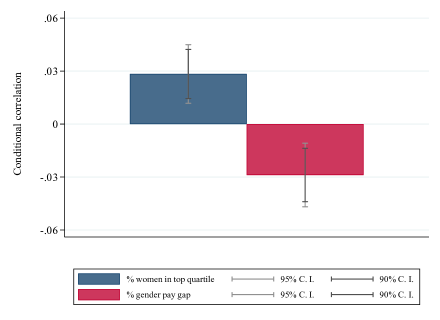
Figure D1: Wage posting and equality indicators - conditional correlations

Potentially, upfront wage information in the recruitment process may help address this gender ask gap by reducing the room for wage bargaining. Interestingly, Flinn and Mullins (2021) show that in a labor market with heterogeneous wage settings, where both wage bargaining and wage posting initially coexist, mandating wage posting reduces the gender pay gap by 6 percent. Also consistent with the hypothesis that wage posting may help address the gender ask gap, when combining the GEO data with the information extracted from BGT vacancies, we find a positive correlation between firms’ wage-posting decision and gender equality performance. Specifically, the bar graph in Appendix Figure D1 reports the correlation between GEO firms’ average percentage of vacancies posting wage information between 2015 and 2019 and, respectively, the average percentage of women in the top quartile of the firm wage distribution (blue bar), and the average gender pay gap (red bar) between 2018 and 2019. When computing these correlations, we control for firms’ 5-digit SIC codes, firms’ size bands, and the occupational composition of vacancies; we also cluster the standard errors at the 5-digit SIC level. The graph shows that firms that are more likely to post wage information also tend to have a larger percentage of women at the top of the firm wage distribution and a lower gender pay gap. While these are only correlations, they further motivate us to study the impact of the transparency policy on firms’ wage-posting decision. For this, we must first introduce the BGT job advert data, how we match these data with other firm-level data to build the difference-in-differences sample, and how we construct the variables of interest.

BGT data.

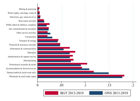
Figure D2: Industry distribution in BGT and ONS Vacancy Survey

BGT scrapes online job ads from company websites and job boards. UK data are available from the 2013 financial year and cover more than 50 million (de-duplicated) individual job vacancies collected from a wide range of online job listing sites. While the data set only includes online advertisements, and hence misses vacancies not posted online (e.g. those advertised informally and internal vacancies), it includes a rich set of information that is especially useful for our analysis. First, each observation includes the text of the job advertisement. Second, more than 95 percent of vacancies have an occupational SOC identifier. Third, around one third of the vacancies, or 17 million observations, include the name of the employer. As this is the only variable that can facilitate the merging of BGT data with other firm-level data, we focus on the restricted sample with non-missing employer names. Importantly, to exclude potential selection issues related to the presence of the firm name, Appendix Figure D2 shows that the industry distribution of the stock of vacancies in BGT and the stock of vacancies in the official ONS Vacancy Survey match well, mitigating concerns regarding the representativeness of BGT.

Difference-in-differences sample.

To implement the difference-in-differences strategy, we need to identify treatment and control groups in BGT, and for this we need to know firms’ number of employees. To retrieve this information, we merge BGT with FAME, the UK version of Amadeus, which is an European firm-level data set managed by Bureau Van Dijk. Appendix Section D explains in detail the name-matching strategy that we use to merge the two data sets, and the additional steps that we take to build the sample for the difference-in-differences analysis. In the final sample, we retain only BGT firms matched with FAME that have a firm size between 200 and 300 employees and non-missing firm size in 2015, the year used to define the treatment status. We also restrict the sample to vacancies with non-missing SOC and SIC codes; and we exclude vacancies for part-time jobs, representing around 10 percent of the sample, to take into account that, when an ad for a part-time job posts a wage, we cannot distinguish whether this is the full-time equivalent or the part-time wage. Finally, in the main specification, we only keep vacancies posted from the fiscal year 2015, as BGT expressed concerned over the quality of the data at the beginning of the sample (Adams et al. 2020).. The final sample includes 97,467 vacancies from 2,556 firms posted over the fiscal years 2015–2019.

BGT outcomes.

To study firms’ wage-posting decision, we extract wages offered from the job-ad text using natural language processing. In particular, to identify wages in the text, we use a series of targeted regular expressions that pick up phrases such as “30-35k per annum” and “20,000/year”. The frequency of the wage offer (annual, weekly, hourly) is similarly inferred from the text, and all values are transformed into annual wages and deflated using the ONS’ 2015 CPI Index. When a vacancy posts a wage interval (46 percent of cases) we consider the mid-point of the interval as the value for the posted wage.

A series of validation exercises conducted by research assistants show that we correctly classify the presence of wages in 98 percent of cases. The residual 2 percent are false negatives, meaning that our code indicates that there is no wage posted when there actually is one. As for the value of posted wages, we correctly identify it in 97 percent of cases. The remaining 3 percent are either the false negatives noted above, or have a typo in the posted wage. Finally, we correctly identify part-time vacancies in 95 percent of cases, with the remaining 5 percent being false positives.

Our main outcome of interest is a dummy variable equal to one if the vacancy contains wage information, either in the form of a wage interval or a point offer. To complement the analysis on wage posting, we also consider the impact of the policy on the posted wage, on whether the vacancy reports a wage interval, and, in case, on its width.

Appendix Table D3 provides summary statistics for the outcomes considered, broken down by treatment status, in the pre-policy period. Note that we define treated firms as in the ASHE analysis, that is, employers with at least 250 employees in 2015. As shown in Table D3, the proportion of full-time vacancies is, respectively, 92 and 90 percent for the treatment and control groups. Focusing on full-time vacancies, treated and control firms post, respectively, 61 and 56 percent of their job ads for higher-paid professions, i.e., managerial, professional, and technical occupations. Treated firms are more likely to post wage information, though the share of vacancies providing wage information remains below 50 percent for both groups (46 vs. 45 percent). As for the characteristics of posted wages, the treatment group has a higher probability of posting a wage interval (51 vs. 41 percent), though the interval dispersion, that is the ratio between the upper and lower bound posted, is similar across the two groups (1.25 vs. 1.23). Also, on average, treated firms offer a lower annual full-time salary in the pre-policy period (£26,000 vs. £29,000). Appendix Figure D4 complements these statistics by showing the occupational and industry distribution of wage posting, separately, for treated and control firms. Across both treatment and control firms, wage posting appears to be more frequent in vacancies for caring and leisure occupations and in the public administration, education and health sectors, which is consistent with evidence from the United States (Hall and Krueger 2012). Also, with few exceptions, the two distributions are similar across the two groups.

BGT analysis.

To study the impact of the policy on firms’ wage posting decision, we estimate the following difference-in-differences model at the vacancy level:

$$Y_{ijt}=\alpha_{j}+\theta_{st}+\beta\left(TreatedFirm_{j}*Post_{t}\right)+u_{ijt},$$ (3)

where $Y_{ijt}$ is either a dummy equal to one if vacancy $i$ of firm $j$ in quarter $t$ offers wage information, the log of the posted wage, whether the firm posts a wage interval, and, if so, the interval dispersion. As in the ASHE analysis, $TreatedFirm_{j}$ is a dummy variable equal to one if a firm has at least 250 employees in 2015; $Post_{t}$ is a dummy variable equal to one from the second quarter of 2018 onward; $\alpha_{j}$ are firm fixed effects; and $\theta_{st}$ are 5-digit SIC-specific quarter fixed effects that control for the potential seasonality of labor demand at industry level ($s$ stands for sector). Finally, we cluster standard errors at the firm level.

Table 4 presents the results of this analysis. First, Column 1 tells us that the policy significantly increases the probability that employers report wage information on their job ads by 4.3 percentage points, or 9 percent compared to the pre-policy sample mean. Panel A of Appendix Figure D5 shows the corresponding event study. While the evolution of wage posting seems comparable across treated and control firms before the introduction of the policy, the share of vacancies posting wage information increases in treated firms compared to control firms after its introduction, with this effect being relatively larger and significant at 1 percent in 2019. In the following columns of Table 4, we complement this analysis by studying whether the policy affects the characteristics of posted wages, including the mean value of wages, whether the firm posts a wage interval, and, where there is an interval, its dispersion. While the policy has no significant impact on the value of posted wages or the probability of posting a wage interval, it significantly decreases the width of intervals that are posted by 4.6 percentage points, or 4 percent relative to the pre-policy mean. In sum, these results show that after the introduction of the policy, employers are more willing to provide upfront wage information, potentially in an effort to reduce the gender pay gap at entry level.

7 Conclusion

To tackle the persistence of gender inequality in the labor market, many governments are introducing pay transparency policies. Exploiting the variation across firm size and over time in the application of the UK’s transparency policy, we show that increased transparency leads to an 18 percent significant reduction in the gender pay gap. Importantly, this effect is the result of a slowdown in men’s wage growth, while the policy has no significant effect on women’s pay. In other words, these results suggest that transparency policies can reduce the gender pay gap with limited costs for firms, but may not be suited to achieve the objective of improving outcomes of lower-paid employees. As an increasing number of studies confirm that transparency policies mainly generate pay compression by pushing down the real wages of better-paid employees (Mas 2017, Bennedsen et al. 2021, Cullen and Pakzad-Hurson 2021, Baker et al. 2022), policy makers should consider whether this is a desirable way to tackle wage inequality.

To conclude, it is important to stress that our analysis only identifies short-term effects. Potentially, pay transparency might only have the effect of stimulating responses from firms in the short run, when it acts as an information shock that attracts strong attention from the public and leads firms to fear for their reputation. If the policy does not produce an actual change in the culture within firms, its effect may fade away over time as the strength of the information shock weakens (Giuliano 2021). In this respect, our analysis of BGT data shows that the UK policy has pushed firms to revise their hiring practices, potentially to reduce the room for wage bargaining. If, over time, this helps firms reduce the gender pay gap at entry level, pay transparency may result in positive long-term effects on gender equality. Considering these ambiguous long-run effects, it is necessary to keep monitoring the impact of these types of policies in order to fully assess their effectiveness.

Figures and Tables

Figure 1: Institutional Setting

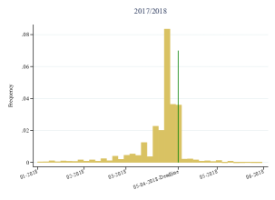
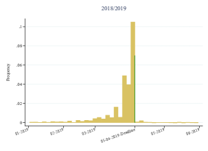
A Distribution of submission dates

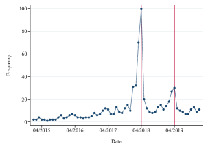
B Google searches for “gender pay gap”

• Source: UK Government Equalities Office (GEO); Google, 2015-2019.

• Notes: The figures in Panel A show the distribution of days when firms published their gender equality indicators. The graph on the left refers to the 2017/18 data (10,557 observations), while the one on the right refers to 2018/19 (10,812 observations). Around 5 percent of firms publish before January of the deadline year. The graph in Panel B reports the UK relative search volume for the term “gender pay gap” between April 2015 and June 2019 using Google’s search services. The frequency is indexed to the peak, which occurred in the week commencing 1st April 2018, when firms faced the first deadline to publish gender equality indicators.

Figure 2: Event studies - log hourly pay

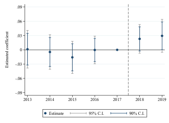
A Gender pay gap

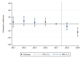
B Men

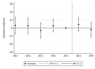
C Women

• Source: ASHE, 2013–2019.

• Notes: These graphs present the estimates of the leads and lags of the policy on the gender pay gap (Panel A), and men’s and women’s pay (Panel B and C, respectively). These results are obtained from the estimation of regression 2. In each graph, the estimation sample includes workers employed in firms with 200 to 300 employees. The graphs also report 90 and 95 percent confidence intervals associated with firm-level clustered standard errors. The dash vertical line indicates the month when the mandate is approved, i.e., February 2017.

Figure 3: Robustness checks - gender pay gap

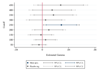
A Placebo regressions

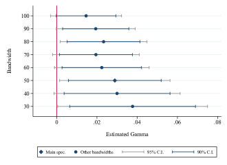
B Changing bandwidth

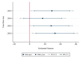
C Changing year treatment status

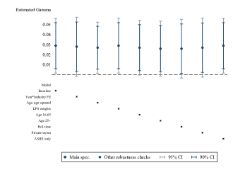
D Other robustness checks

• Source: ASHE, 2013–2019.

• Notes: These graphs present a series of robustness checks on the impact of the policy on the gender pay gap. Detailed results are presented in Appendix Tables A5-A8.

Table 1: Public gender equality indicators

	2017/18	2018/19
	(1)	(2)
Gender median hourly pay gap (%)	11.79	11.88
	(15.84)	(15.51)
Gender mean hourly pay gap (%)	14.33	14.19
	(14.91)	(14.21)
Gender median bonus gap (%)	-21.72	-0.86
	(1,399.04)	(270.51)
Gender mean bonus gap (%)	7.66	15.44
	(833.06)	(200.70)
% men receiving bonus	35.39	35.72
	(36.33)	(36.68)
% women receiving bonus	33.92	34.40
	(36.01)	(36.38)
% women lower quartile	53.67	53.88
	(24.13)	(24.11)
% women lower-middle quartile	49.49	49.82
	(26.09)	(26.19)
% women upper-middle quartile	45.15	45.62
	(26.22)	(26.32)
% women top quartile	39.20	39.75
	(24.41)	(24.48)
Observations	10,557	10,812

• Source: UK Government Equalities Office (GEO).

• Notes: This table reports mean and standard deviation of gender equality indicators published by targeted firms, separately by year of publication.

Table 2: ASHE Summary statistics - pre-policy period

	Treated men	Control men	Treated women	Control women
	(1)	(2)	(3)	(4)
Hourly pay (£)	15.93	15.59	13.36	13.40
	(14.24)	(11.68)	(8.87)	(10.70)
Weekly pay (£)	581.51	569.38	414.60	411.69
	(533.28)	(429.76)	(307.32)	(316.98)
Weekly hours	36.41	36.67	30.69	30.49
	(8.53)	(8.50)	(10.53)	(10.69)
Receiving allowances/bonuses	0.29	0.29	0.19	0.18
	(0.45)	(0.46)	(0.39)	(0.38)
Allowance/bonus amount (£)	26.03	26.08	10.07	9.47
	(102.33)	(114.65)	(38.71)	(42.15)
Promotion	0.03	0.03	0.04	0.04
	(0.17)	(0.18)	(0.18)	(0.18)
Managerial occupation	0.10	0.10	0.07	0.06
	(0.30)	(0.30)	(0.26)	(0.24)
Highest-paid occupations	0.42	0.42	0.40	0.37
	(0.49)	(0.49)	(0.49)	(0.48)
Tenure in months	87.40	86.28	74.37	72.10
	(98.47)	(96.65)	(80.85)	(80.34)
Leaving firm in t+1	0.36	0.35	0.37	0.35
	(0.48)	(0.48)	(0.48)	(0.48)
Private sector	0.91	0.92	0.80	0.78
	(0.29)	(0.27)	(0.40)	(0.41)
Covered by collective agreement	0.28	0.27	0.32	0.34
	(0.45)	(0.44)	(0.47)	(0.47)
Observations	6,916	8,677	5,870	7,711

• Source: ASHE, 2013–2017.

• Notes: This table reports mean and standard deviation of the main variables used in the analysis, separately for men and women, and treatment and control group, before the implementation of the mandate.

Table 3: Impact on pay outcomes

	Log hourly	Log hourly	Allowances	Promotion
	pay	basic pay	& bonuses
	(1)	(2)	(3)	(4)
Treated firm*post	-0.026∗∗∗	-0.024∗∗∗	-0.025	-0.002
	(0.008)	(0.009)	(0.024)	(0.008)
Treated firm*post*fem	0.029∗∗	0.031∗∗	0.002	0.011
	(0.014)	(0.014)	(0.032)	(0.011)
Observations	29,226	29,226	29,226	29,226
Adjusted $R^{2}$	0.909	0.911	0.622	0.003
P-value Women Coeff	0.788	0.578	0.306	0.281
Men’s pre-policy mean	15.93	15.25	0.68	0.03
Women’s pre-policy mean	13.36	13.02	0.34	0.04

• Source: ASHE, 2013–2019.

• Notes: This table reports the impact of pay transparency on pay outcomes, obtained from the estimation of regression 1. Each column refers to a different outcome, as specified at the top of it. The estimation sample comprises men and women working in firms that have between 200 and 300 employees. All regressions include firm*individual fixed effects, gender*year fixed effects, and region-specific time shocks. A treated firm is defined as having at least 250 employees in 2015. The post dummy is equal to one from 2018 onward. Heteroskedasticity-robust standard errors clustered at firm level in parentheses. The p-value at the bottom of the table refers to the t-test on the sum of the two reported coefficients, corresponding to the effect of the policy on female employees. The pre-policy mean represents the mean of the outcome variable for the treated group between 2013 and 2017.

• *** p$<$0.01, ** p$<$0.05, * p$<$0.1.

Table 4: Impact on wage-posting decision

	Wage	Log annual	Wage	Interval
	posted	wage	interval	dispersion
	(1)	(2)	(3)	(4)
Treated firm*post	0.043∗	0.040	0.036	-0.046∗
	(0.022)	(0.029)	(0.028)	(0.026)
Observations	97,467	43,752	43,752	19,342
Adjusted $R^{2}$	0.470	0.584	0.414	0.382
Pre-policy mean	0.46	26,116	0.51	1.25

• Source: BGT, 2015–2019.

• Notes: This table reports the impact of pay transparency on firms’ decision to post wage information in job vacancies and on the characteristics of posted wages, obtained from the estimation of regression 3. The estimation sample comprises BGT firms that have between 200 and 300 employees. In Column 2, it is restricted to vacancies with wage information. In Column 4, it is further restricted to vacancies posting a wage interval. All regressions include firm fixed effects and 5-digit SIC-specific time shocks. A treated firm is defined as having at least 250 employees in 2015. The post dummy is equal to one from the second quarter of 2018 onward. Heteroskedasticity-robust standard errors clustered at firm level in parentheses. The pre-policy mean represents the mean of the outcome variable for the treated group between 2015 and 2017.

• *** p$<$0.01, ** p$<$0.05, * p$<$0.1.

Appendix

Appendix A Further results and robustness checks

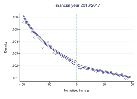
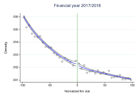
Figure A1: Firm size distribution

Source: BSD, 2016–2018.
Note: These graphs show the distribution of firms around the 250-employee cutoff in each year since the announcement of the policy. In each figure, the sample includes firms with +/100 employees from the threshold, grouped in 20 bins. Each dot represents the share of firms with a number of employees comprised in the corresponding bin.

Figure A2: Event studies - other pay outcomes

       

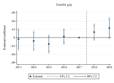
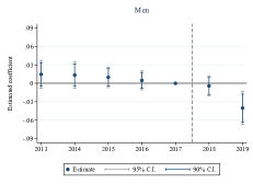
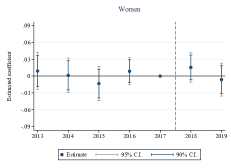
A Log hourly basic pay

       

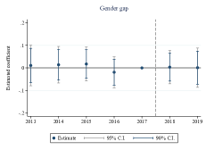
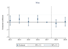
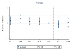
B Allowances and bonuses

       

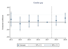
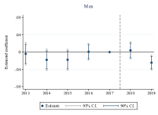
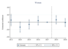
C Promotion

Source: ASHE, 2013–2019.
Notes: These graphs present the estimates of the leads and lags of the policy on different pay outcomes. These results are obtained from the estimation of regression 2. In each graph, the estimation sample includes workers employed in firms with 200 to 300 employees. The graphs also report 90 and 95 percent confidence intervals associated with firm-level clustered standard errors. The dash vertical line indicates the month when the mandate is approved, i.e., February 2017.

Figure A3: Unconditional trends in men’s basic pay

   

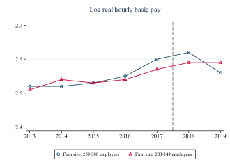
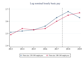
A Men’s real vs. nominal pay

   

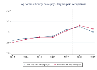
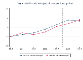
B Men’s nominal pay - higher vs. lower paid occupations

Source: ASHE, 2013–2019.
Notes: The graphs in Panel A present the unconditional trends in men’s log real and nominal basic pay, separately for treatment and control groups. The graphs in Panel B further compare trends in nominal basic pay across higher and lower-paid occupations. Higher paid occupations include managerial, professional, and technical occupations (1-digit SOC 1-3), while lower paid occupations, i.e. administrative, skilled-trades, caring and leisure, sales and customer service, plant and machine operative, and elementary occupations (1-digit SOC 4-9). In each graph, the blue line represents the treatment group, individuals working in firms with 250-300 employees, and the red line the control group, individuals working in firms with 200-249 employees. The dash vertical line indicates the month when the mandate is approved, i.e., February 2017.

Figure A4: Unconditional trends in women’s basic pay

   

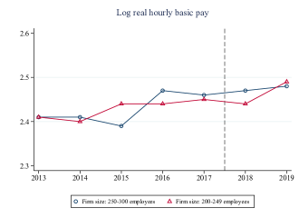
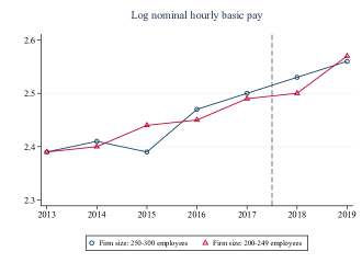
A Women’s real vs. nominal pay

   

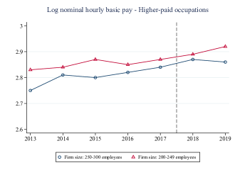
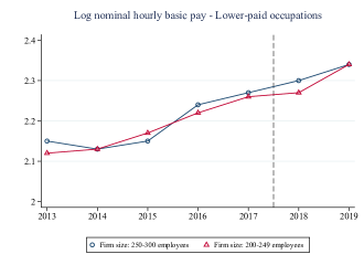
B Women’s nominal pay - higher vs. lower paid occupations

Source: ASHE, 2013–2019.
Notes: The graphs in Panel A present the unconditional trends in women’s log real and nominal basic pay, separately for treatment and control groups. The graphs in Panel B further compare trends in nominal basic pay across higher and lower-paid occupations. Higher paid occupations include managerial, professional, and technical occupations (1-digit SOC 1-3), while lower paid occupations, i.e. administrative, skilled-trades, caring and leisure, sales and customer service, plant and machine operative, and elementary occupations (1-digit SOC 4-9). In each graph, the blue line represents the treatment group, individuals working in firms with 250-300 employees, and the red line the control group, individuals working in firms with 200-249 employees. The dash vertical line indicates the month when the mandate is approved, i.e., February 2017.

Figure A5: Estimation sample versus entire ASHE

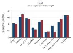
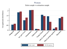
A Occupational distribution

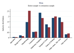
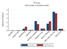
B Industry distribution

Source: ASHE, 2013–2019.
Note: These figures compare the occupational and industry distributions of men and women in the estimation sample and in the entire population of ASHE, over the period of analysis.

Table A1: Impact on log hourly pay - extending treatment period

	2013-19	2013-20	2013-21
	(1)	(2)	(3)
Treated firm*post	-0.026∗∗∗	-0.028∗∗∗	-0.029∗∗∗
	(0.008)	(0.009)	(0.009)
Treated firm*post*fem	0.029∗∗	0.031∗∗	0.030∗∗
	(0.014)	(0.014)	(0.013)
Observations	29,226	33,421	35,123
Adjusted $R^{2}$	0.909	0.897	0.894
P-value Women Coeff	0.788	0.785	0.909
Men’s pre-policy mean	2.58	2.58	2.58
Women’s pre-policy mean	2.45	2.45	2.45

• Source: ASHE, 2013–2021.

• Notes: This table reports the impact of pay transparency on employees’ hourly pay, obtained from the estimation of regression 1. Each column refers to a different estimation period, as specified at the top of it. The estimation sample comprises men and women working in firms that have between 200 and 300 employees. All regressions include firm*individual fixed effects, gender*year fixed effects, and region-specific time shocks. A treated firm is defined as having at least 250 employees in 2015. The post dummy is equal to one from 2018 onward. Heteroskedasticity-robust standard errors clustered at firm level in parentheses. The p-value at the bottom of the table refers to the t-test on the sum of the two reported coefficients, corresponding to the effect of the policy on female employees. The pre-policy mean represents the mean of the outcome variable for the treated group between 2013 and 2017.

• *** p$<$0.01, ** p$<$0.05, * p$<$0.1.

Table A2: Impact on job mobility

	Tenure	Leaving the firm	Managerial
	in months	in t+1	occupation
	(1)	(2)	(3)
Treated firm*post	-0.542	-0.002	-0.001
	(0.736)	(0.024)	(0.008)
Treated firm*post*fem	0.580	0.021	0.006
	(1.008)	(0.034)	(0.011)
Observations	29,226	28,714	29,226
Adjusted $R^{2}$	0.989	0.111	0.898
P-value Women Coeff	0.957	0.497	0.466
Men’s pre-policy mean	87.40	0.36	0.10
Women’s pre-policy mean	74.37	0.37	0.07

• Source: ASHE, 2013–2019.

• Notes: This table reports the impact of pay transparency on job mobility, obtained from the estimation of regression 1. Each column refers to a different outcome, as specified at the top of it. The estimation sample comprises men and women working in firms that have between 200 and 300 employees. All regressions include firm*individual fixed effects, gender*year fixed effects, and region-specific time shocks. A treated firm is defined as having at least 250 employees in 2015. The post dummy is equal to one from 2018 onward. Heteroskedasticity-robust standard errors clustered at firm level in parentheses. The p-value at the bottom of the table refers to the t-test on the sum of the two reported coefficients, corresponding to the effect of the policy on female employees. The pre-policy mean represents the mean of the outcome variable for the treated group between 2013 and 2017.

• *** p$<$0.01, ** p$<$0.05, * p$<$0.1.

Table A3: Impact on pay and hours worked

	Log hourly	Log weekly	Weekly	Part-time
	pay	pay	hours
	(1)	(2)	(3)	(4)
Treated firm*post	-0.026∗∗∗	-0.019∗	0.084	-0.001
	(0.008)	(0.010)	(0.009)	(0.009)
Treated firm*post*fem	0.029∗∗	0.010	-0.461	0.016
	(0.014)	(0.018)	(0.371)	(0.016)
Observations	29,226	29,226	29,226	29,226
Adjusted $R^{2}$	0.909	0.913	0.798	0.752
P-value Women Coeff	0.788	0.532	0.242	0.340
Men’s pre-policy mean	15.93	581.51	36.41	0.10
Women’s pre-policy mean	13.36	414.60	30.69	0.34

• Source: ASHE, 2013–2019.

• Notes: This table reports the impact of pay transparency on pay outcomes and hours worked, obtained from the estimation of regression 1. Each column refers to a different outcome, as specified at the top of it. The estimation sample comprises men and women working in firms that have between 200 and 300 employees. All regressions include firm*individual fixed effects, gender*year fixed effects, and region-specific time shocks. A treated firm is defined as having at least 250 employees in 2015. The post dummy is equal to one from 2018 onward. Heteroskedasticity-robust standard errors clustered at firm level in parentheses. The p-value at the bottom of the table refers to the t-test on the sum of the two reported coefficients, corresponding to the effect of the policy on female employees. The pre-policy mean represents the mean of the outcome variable for the treated group between 2013 and 2017.

• *** p$<$0.01, ** p$<$0.05, * p$<$0.1.

Table A4: Impact on pay outcomes by occupation

	Log hourly pay			Promotion
	Entire	Lower	Higher	Entire	Lower	Higher
	sample	paid	paid	sample	paid	paid
	(1)	(2)	(3)	(4)	(5)	(6)
Treated firm*post	-0.026∗∗∗	-0.020∗	-0.030∗∗	-0.002	-0.002	-0.002
	(0.008)	(0.010)	(0.014)	(0.008)	(0.010)	(0.012)
Treated firm*post*fem	0.029∗∗	0.017	0.046∗∗	0.011	0.006	0.013
	(0.014)	(0.018)	(0.022)	(0.011)	(0.014)	(0.019)
Observations	29,226	16,623	12,082	29,226	16,623	12,082
Adjusted $R^{2}$	0.909	0.776	0.904	0.003	0.025	-0.016
P-value Women Coeff	0.788	0.868	0.405	0.281	0.701	0.540
P-value High vs. Low M		0.554			0.968
P-value High vs. Low W		0.443			0.747
Men’s pre-policy mean	15.93	10.51	23.53	0.03	0.03	0.03
Women’s pre-policy mean	13.36	9.73	18.87	0.04	0.03	0.05

• Source: ASHE, 2013–2019.

• Notes: This table compares the impact of pay transparency on employees’ hourly pay and the probability of getting promoted across occupations, by estimating regression 1 by subgroup. Column 1 (4) reports the estimate on log hourly pay (promotion) for the entire sample, employees working in firms that have between 200 and 300 employees. Columns 2 (5) and 3 (5) compare the impact across lower and higher-paid occupations, where this grouping is based on the ranking of pre-policy 1-digit SOC-specific median wages. All regressions include firm*individual fixed effects, gender*year fixed effects, and region-specific time shocks. A treated firm is defined as having at least 250 employees in 2015. The post dummy is equal to one from 2018 onward. Heteroskedasticity-robust standard errors clustered at firm level in parentheses. The “ P-value Women Coeff” refers to the t-test on the sum of the two reported coefficients, corresponding to the effect of the policy on female employees. The “P-value High vs. Low M (W)” refers to the t-test on the equality of effects on men’s (women’s) pay across occupations. The pre-policy mean represents the mean of the outcome variable for the treated group and subgroup considered between 2013 and 2017.

• *** p$<$0.01, ** p$<$0.05, * p$<$0.1.

Table A5: Impact on log hourly pay - placebo regressions

	50	100	150	200	250	300	350	400	450
	(1)	(2)	(3)	(4)	(5)	(6)	(7)	(8)	(9)
Treated firm*post	-0.005	-0.009	-0.003	-0.006	-0.026∗∗∗	-0.011	-0.013	0.001	-0.012
	(0.004)	(0.006)	(0.007)	(0.008)	(0.008)	(0.010)	(0.010)	(0.012)	(0.016)
Treated firm*post*fem	-0.005	0.005	-0.002	0.006	0.029∗∗	0.005	0.017	0.015	0.028
	(0.006)	(0.009)	(0.010)	(0.013)	(0.014)	(0.015)	(0.018)	(0.018)	(0.021)
Observations	243,795	85,204	52,438	39,429	29,226	22,964	19,406	15,994	13,616
Adjusted $R^{2}$	0.866	0.899	0.905	0.908	0.909	0.912	0.912	0.908	0.909
P-value Women Coeff	0.044	0.548	0.543	0.995	0.788	0.638	0.783	0.239	0.301
Men’s pre-policy mean	14.86	15.36	15.80	15.71	15.93	15.66	16.03	16.04	16.05
Women’s pre-policy mean	11.99	12.79	12.87	13.49	13.36	13.53	13.04	13.50	13.06

• Source: ASHE, 2013–2019.

• Notes: This table reports the impact of placebo policies on log hourly pay, obtained from the estimation of regression 1. In each regression, the estimation sample comprises employees working in firms that have +/- 50 employees from the threshold $c$ specified at the top of each column. All regressions include firm*individual fixed effects, gender*year fixed effects, and region-specific time shocks. A treated firm is defined as having at least 250 employees in 2015. The post dummy is equal to one from 2018 onward. Heteroskedasticity-robust standard errors clustered at firm level in parentheses. The p-value at the bottom of the table refers to the t-test on the sum of the two reported coefficients, corresponding to the effect of the policy on female employees. The pre-policy mean represents the mean of the outcome variable for the treated group between 2013 and 2017.

• *** p$<$0.01, ** p$<$0.05, * p$<$0.1.

Table A6: Impact on log hourly pay - different bandwidths

	30	40	50	60	70	80	90	100
	(1)	(2)	(3)	(4)	(5)	(6)	(7)	(8)
Treated firm*post	-0.020∗	-0.020∗∗	-0.026∗∗∗	-0.022∗∗∗	-0.023∗∗∗	-0.024∗∗∗	-0.019∗∗∗	-0.018∗∗∗
	(0.011)	(0.010)	(0.008)	(0.008)	(0.007)	(0.007)	(0.006)	(0.006)
Treated firm*post*fem	0.038∗∗	0.030∗	0.029∗∗	0.022∗	0.019∗	0.023∗∗	0.019∗	0.015
	(0.019)	(0.016)	(0.014)	(0.012)	(0.011)	(0.011)	(0.010)	(0.009)
Observations	15,867	22,533	29,226	36,201	43,478	50,693	58,291	66,553
Adjusted $R^{2}$	0.909	0.911	0.909	0.907	0.909	0.908	0.908	0.908
P-value Women Coeff	0.249	0.444	0.788	0.979	0.662	0.952	0.961	0.629
Men’s pre-policy mean	16.08	16.13	15.93	15.78	15.87	15.88	15.83	15.83
Women’s pre-policy mean	13.37	13.37	13.36	13.37	13.46	13.45	13.43	13.40

• Source: ASHE, 2013–2019.

• Notes: This table reports the impact of pay transparency on log hourly pay, obtained from the estimation of regression 1. In each regression, the estimation sample comprises individuals working in firms that have +/- $h$ employees from the 250-employee threshold, where $h$ is indicated at the top of each column. All regressions include firm*individual fixed effects, gender*year fixed effects, and region-specific time shocks. A treated firm is defined as having at least 250 employees in 2015. The post dummy is equal to one from 2018 onward. Heteroskedasticity-robust standard errors clustered at firm level in parentheses. The p-value at the bottom of the table refers to the t-test on the sum of the two reported coefficients, corresponding to the effect of the policy on female employees. The pre-policy mean represents the mean of the outcome variable for the treated group between 2013 and 2017.

• *** p$<$0.01, ** p$<$0.05, * p$<$0.1.

Table A7: Impact on log hourly pay - changing year to define treatment status

	Main	Firm size	Firm size	Firm size
	spec	2014	2013	2012
	(1)	(2)	(3)	(4)
Treated firm*post	-0.026∗∗∗	-0.020∗∗	-0.019∗∗	-0.032∗∗∗
	(0.008)	(0.009)	(0.008)	(0.009)
Treated firm*post*fem	0.029∗∗	0.017	0.028∗	0.033∗∗
	(0.014)	(0.015)	(0.014)	(0.015)
Observations	29,226	29,030	28,765	28,378
Adjusted $R^{2}$	0.909	0.908	0.908	0.908
P-value Women Coeff	0.788	0.804	0.462	0.938
Men’s pre-policy mean	15.93	15.80	16.09	16.21
Women’s pre-policy mean	13.36	13.44	13.40	13.25

• Source: ASHE, 2013–2019.

• Notes: This table reports the impact of pay transparency on log hourly pay, obtained from the estimation of regression 1. In each regression, the estimation sample comprises men and women working in firms that have between 200 and 300 employees. All regressions include firm*individual fixed effects, gender*year fixed effects, and region-specific time shocks. A treated firm is defined as having at least 250 employees in 2015 or in the year indicated on top of each column. The post dummy is equal to one from 2018 onward. Heteroskedasticity-robust standard errors clustered at firm level in parentheses. The p-value at the bottom of the table refers to the t-test on the sum of the two reported coefficients, corresponding to the effect of the policy on female employees. The pre-policy mean represents the mean of the outcome variable for the treated group between 2013 and 2017.

• *** p$<$0.01, ** p$<$0.05, * p$<$0.1.

Table A8: Impact on log hourly pay - other robustness checks

	Main	1-digit SIC	Age	LFS	25	16-65	Private	Full-time	ASHE
	spec	FE	controls	weights	+		sector		only
	(1)	(2)	(3)	(4)	(5)	(6)	(7)	(8)	(9)
Treated firm*post	-0.026∗∗∗	-0.026∗∗∗	-0.020∗∗	-0.026∗∗∗	-0.019∗∗	-0.026∗∗∗	-0.028∗∗∗	-0.021∗∗∗	-0.025∗∗∗
	(0.008)	(0.009)	(0.008)	(0.009)	(0.008)	(0.009)	(0.009)	(0.008)	(0.009)
Treated firm*post*fem	0.029∗∗	0.028∗∗	0.027∗∗	0.029∗∗	0.026∗	0.027∗	0.027∗	0.026∗	0.029∗∗
	(0.014)	(0.014)	(0.013)	(0.014)	(0.014)	(0.014)	(0.015)	(0.015)	(0.014)
Observations	29,226	29,226	29,220	29,226	26,695	28,561	24,984	23,084	25,845
Adjusted $R^{2}$	0.909	0.909	0.912	0.915	0.916	0.908	0.910	0.935	0.912
Firm*Ind FE	✓	✓	✓	✓	✓	✓	✓	✓	✓
Year*Reg FE	✓		✓	✓	✓	✓	✓	✓	✓
Year*SIC1 FE		✓
P-value Women Coeff	0.788	0.868	0.526	0.761	0.576	0.916	0.991	0.713	0.731
Men’s pre-policy mean	15.93	15.93	15.93	17.07	16.83	15.97	15.88	16.48	16.03
Women’s pre-policy mean	13.36	13.36	13.36	13.88	14.05	13.39	13.03	14.05	13.36

• Source: ASHE, 2013–2019.

• Notes: This table reports a series of robustness checks on the impact of pay transparency on log hourly pay, obtained from the estimation of regression 1. In each regression, the estimation sample comprises men and women working in firms that have between 200 and 300 employees. A treated firm is defined as having at least 250 employees in 2015. The post dummy is equal to one from 2018 onward. All regressions include firm*individual fixed effects, gender*year fixed effects, and region-specific time shocks – with the exception of Column 2 that controls for 1-digit SIC-specific time shocks. Heteroskedasticity- robust standard errors clustered at firm level in parentheses. The p-value at the bottom of the table refers to the t-test on the sum of the two reported coefficients, corresponding to the effect of the policy on female employees. The pre-policy mean represents the mean of the outcome variable for the treated group between 2013 and 2017.

• *** p$<$0.01, ** p$<$0.05, * p$<$0.1.

Appendix B Mechanisms

B.1 Performance comparisons

Table B1: 2018 Gender pay gap and changes in employees’ pay

	% $\Delta$	% $\Delta$	% $\Delta$
	Gender pay gap	Men’s pay	Women’s pay
	(1)	(2)	(3)
2018 Gender pay gap	-1.665∗∗∗	-0.057∗	0.050∗
	(0.111)	(0.032)	(0.030)
Observations	9,599	4,163	3,890

• Source: UK Government Equalities Office (GEO), ASHE 2018-2019.

• Notes: This table shows the correlation between the publicly available 2018 gender median hourly pay gap and 2018-19 changes in, respectively, the firm’s gender pay gap, men’s and women’s median hourly pay. All regressions control for 5-digit SIC fixed effects. The sample in Column 1 includes 9,599 firms that publish gender equality indicators in both 2018 and 2019. Columns 2 and 3 include the subgroup of these firms that are also present in ASHE in 2018 and 2019 with either male or female employees (respectively 4,163 and 3,890 firms). In all regressions, outliers (the bottom and top 1 percent) in the distribution of the y variable are excluded. Standard errors are clustered at the level of 5-digit SIC.

B.2 YouGov data and firms’ reputation

Figure B1: YouGov vs. GEO sample

A Firm-size distribution

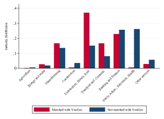
B Industry distribution

Source: UK Government Equality Office (GEO), YouGov 2018-2019.
Note: These figures compare the firm-size and industry distributions in the YouGov-GEO matched sample and in the entire GEO sample.

Table B2: Gender equality performance and presence in YouGov

	2017/18				2018/19
	Entire	Matched with YouGov		P-value	Entire	Matched with YouGov		P-value
	sample	Yes	No	difference	sample	Yes	No	difference
	(1)	(2)	(3)	(4)	(5)	(6)	(7)	(8)
Gender pay gap (%)	11.79	12.92	11.73	0.09	11.88	12.37	11.85	0.46
	(15.84)	(13.80)	(15.94)		(15.51)	(13.38)	(15.61)
Observations	10,557	540	10,017		10,812	527	10,285

• Source: GEO, YouGov 2018–2019.

• Notes: This table explores potential selection patterns of GEO firms matched with YouGov. Column 1 (5) reports the gender median hourly pay gap for all GEO firms in 2017/2018 (2018/2019); Column 2 (6) refers to firms matched with YouGov; Column 3 (7) refers to firms that we do not find in YouGov; Column 4 (8) reports the p-value of the difference in the sample means of these two groups.

• *** p$<$0.01, ** p$<$0.05, * p$<$0.1.

Table B3: Gender pay gap and placement in YouGov Rankings

	Women’s Rankings	Workforce Rankings
	(1)	(2)
Gender pay gap	-0.672∗	-0.794∗∗
	(0.378)	(0.373)
Observations	1,830	1,836
Year FE	✓	✓
GEO firm FE	✓	✓

• Source: UK Government Equalities Office (GEO), YouGov, 2018–2019.

• Notes: This table shows the correlation between firms’ gender median hourly pay gap and, respectively, firms’ placement in YouGov Women’s Rankings (Column 1), and YouGov Workforce Rankings (Column 2). The gender pay gap is expressed relative to men’s pay. Firms’ placement in YouGov Rankings is measured such that a smaller number indicates a lower position in the ranking. In each column, the sample includes YouGov Rankings’ firms that either publish directly or have a parent company that publishes gender equality indicators in at least one year. Each year, data for YouGov Women’s rankings are missing for 3 firms, compared to the list of employers included in YouGov Workforce Rankings. Standard errors are clustered at the level of the GEO company.

• *** p$<$0.01, ** p$<$0.05, * p$<$0.1.

B.3 Firms’ response to public scrutiny

Table B4: Impact on log hourly pay by industry

	Entire sample	Low exposure	High exposure
	(1)	(2)	(3)
Treated firm*post	-0.026∗∗∗	-0.016∗	-0.052∗∗∗
	(0.008)	(0.010)	(0.017)
Treated firm*post*fem	0.029∗∗	0.030∗	0.050∗
	(0.014)	(0.016)	(0.026)
Observations	29,226	18,900	10,189
Adjusted $R^{2}$	0.909	0.902	0.918
P-value Women Coeff	0.788	0.322	0.903
P-value High vs. Low M		0.056
P-value High vs. Low W		0.527
Men’s pre-policy mean	15.93	15.56	16.39
Women’s pre-policy mean	13.36	13.30	13.46

• Source: ASHE, 2013–2019.

• Notes: This table compares the impact of pay transparency on employees’ hourly pay across industries, by estimating regression 1 by subgroup. The first column reports the estimate for the entire sample, employees working in firms that have between 200 and 300 employees. Columns 2 and 3 compare the impact across industries that are less or more exposed to publicly scrutiny, based on their presence in YouGov surveys (see Section 5 for the definition of these two groups). All regressions include firm*individual fixed effects, gender*year fixed effects, and region-specific time shocks. A treated firm is defined as having at least 250 employees in 2015. The post dummy is equal to one from 2018 onward. Heteroskedasticity-robust standard errors clustered at firm level in parentheses. The “ P-value Women Coeff” refers to the t-test on the sum of the two reported coefficients, corresponding to the effect of the policy on female employees. The “P-value High vs. Low M (W)” refers to the t-test on the equality of effects on men’s (women’s) pay across industries. The pre-policy mean represents the mean of the outcome variable for the treated group and subgroup considered between 2013 and 2017.

• *** p$<$0.01, ** p$<$0.05, * p$<$0.1.

Appendix C Firms’ profits

Our analysis shows that pay transparency pushes firms to reduce men’s pay growth. A natural question to ask is whether this reduction of the wage bill translates into higher profits. Answering this question is important to assess the overall welfare implications of pay transparency policy. Moreover, the answer to this question is not obvious, as many studies outside of the gender literature show that pay transparency policies have a priori ambiguous effects on workers’ productivity (Card et al. 2012, Breza et al. 2018, Dube et al. 2019, Cullen and Perez-Truglia 2021.). On the one hand, learning about pay inequality in the workplace may decrease the job satisfaction and productivity of lower paid employees, while the higher-paid may feel threatened by any attempt of the employer to mitigate inequality. On the other hand, if firms respond to the policy by improving gender equality, this could boost the productivity of those workers who care about working in a fair environment.

While the data available do not allow us to rigorously estimate the impact of the policy on labour productivity, in Table C1, we study its implications for firms’ wage bill and profits by estimating the following difference-in-differences model on the sample of firms with +/- 50 employees from the 250-employee cutoff:

$$Y_{jt}=\alpha_{j}+\theta_{t}+\beta(TreatedFirm_{j}*Post_{t})+Z_{jt}^{\prime}\delta+u_{jt},$$ (C.1)

where $Y_{jt}$ is either labor costs or profits of firm $j$ in year $t$; $\alpha_{j}$ and $\theta_{t}$ are firm and year fixed effects respectively, and $Z_{jt}$ includes region-specific time shocks. As in the ASHE analysis, $TreatedFirm_{j}$ is a dummy equal to one if a firm has at least 250 employees in 2015, and $Post_{t}$ is a dummy equal to one from the second quarter of 2018 onward. Standard errors are clustered at the firm level.

For this part of the analysis, we use the Annual Business Survey (ABS),, an annual survey of businesses covering the production, construction, distribution, and service industries, which represent about two-thirds of the UK economy in terms of gross value added (GVA). We measure labor costs using the log of wage costs, and consider the inverse hyperbolic transformation of GVA to account for negative profits. All monetary values are deflated using the ONS 2015 CPI Index.

Table C1 offers two insights. First, in line with the negative effect that we find on men’s pay, the policy leads to a significant reduction in firms’ wage bill. Second and despite this, the policy has no impact on firms’ profits, which points to a negative effect on employees’ productivity. The studies cited above show that pay transparency reduces workers’ effort only when these cannot assess what determines pay differentials across colleagues (Card et al. 2012, Dube et al. 2019). In contrast, when workers can clearly perceive that their higher-paid peers are more productive than themselves, learning about pay disparity has no detrimental impact on their effort (Breza et al. 2018, Cullen and Perez-Truglia 2021). As discussed in Section 1, the fact that the UK transparency policy imposes firms to publish only their raw gender pay gap, rather than pay gaps within profession and hierarchy position, does not allow to distinguish what part of the gap is due to occupation or experience differences across genders, and what part could instead depend on factors such as explicit discrimination, subtle discrimination, or implicit biases. In turn, this opacity of the transparency indicators may contribute to explain the likely detrimental effect on workers’ productivity.

Figure C1: Event studies - firm-level outcomes

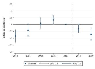
A Wage costs

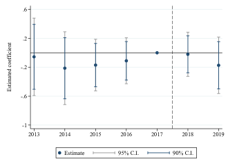
B Profits

Source: ABS, 2013–2019.
Notes: These graphs present the estimates of the leads and lags of the policy on firm-level outcomes. These results are obtained from the estimation of the dynamic version of regression C.1. In each graph, the estimation sample includes firms with 200 to 300 employees. The graphs also report 90 and 95 percent confidence intervals associated with firm-level clustered standard errors. The dash vertical line indicates the month when the mandate is approved, i.e., February 2017.

Table C1: Impact on firm-level outcomes

	Wage costs	Profits
	(1)	(2)
Treated firm*post	-0.050∗∗∗	-0.002
	(0.015)	(0.137)
Observations	10,397	10,397
Adjusted $R^{2}$	0.858	0.695
Pre-policy mean	8.78	8.86

• Source: ABS 2013–2019.

• Notes: This table reports the impact of pay transparency on firms’ profits and labor costs, obtained from the estimation of regression C.1. Each column refers to a different outcome, as specified at the top of it. The estimation sample comprises firms that have between 200 and 300 employees. All regressions include year and firm fixed effects, and region-specific time shocks. A treated firm is defined as having at least 250 employees in 2015. The post dummy is equal to one from 2018 onward. Heteroskedasticity-robust standard errors clustered at firm level in parentheses. The pre-policy mean represents the mean of the outcome variable for the treated group between 2013 and 2017.

• *** p$<$0.01, ** p$<$0.05, * p$<$0.1.

Appendix D Burning Glass Technologies data

D.1 Name matching algorithm

We merge two different firm-level data sets, A and B, through the only common identifier available: firm name. We first collapse all firm names in each data set down to a unique set of firm names using standard text cleaning procedures; this includes dropping any exact duplicates. We then use firm names from one of the datasets, A, to define a vector space using all character-level 1–4-grams (with a maximum of 30,000 features) to create a matrix with dimensions number of entries in A times number of text features. This is achieved using Python’s scikit-learn’s (Pedregosa et al., 2011) TF-IDF Vectorizer, so that frequently appearing 1–4 character grams are down-weighted. As the final stage of preparation for matching, the cleaned firm names in B are expressed in the vector space defined by the cleaned firm names from A.

To perform the matching, we use cosine similarity. Note that this involves taking the inner vector product of every firm name in A with every firm name in B so is computationally intensive. To facilitate this, we use the sparse_dot_topn package, developed by ING Bank, to perform parallel computation of the closest matches across A and B.

The result is an array of scores of the firm name matches between A and B that we are then able to use at different thresholds according to how close a match we prefer, with unity reflecting a perfect match in the vector space, and 0 reflecting two firm names that are entirely orthogonal in the vector space.

D.2 GEO firms in BGT

In order to explore correlations between firms’ hiring practices and gender equality indicators, we match GEO firms with BGT using the name-matching strategy explained above. We retain only employers with a match score of one, for a total of 6,852 GEO firms, of which 5,107 publish gender equality indicators in both 2017/18 and 2018/19 and have non-missing SIC and SOC codes. Table D1 explores selection patterns of the matched sample. While GEO firms matched with BGT have, on average, a larger and statistically different gender pay gap in both years than firms that do not match with BGT, the percentage of women in the top quartile of the firm wage distribution is not statistically different across the two groups.

D.3 Difference-in-differences sample

To implement the difference-in-differences strategy, we need to identify a treatment and a control group in BGT, and for this we need information on firms’ number of employees. We now describe in detail how we create this sample, putting particular care in explaining why we need to exclude some firms at each stage, and what impact this could have in terms of sample selection.

FAME.

We start from FAME, the UK version of Amadeus, covering all UK-registered firms. For around 30 percent of them we have information on the number of employees for at least one year in the pre-policy period. To address selectivity concerns at this stage, in Figure D3 we compare the industry distribution for firms with and without information on the number of employees in 2015, the year used to define the treatment status. Reassuringly, while firms with missing information on employees’ numbers also tend to have missing information on industry, the rest of the distribution appears similar. At this stage, we retain all FAME firms with a number of employees between 200 and 300 in at least one year and non-missing firm size in 2015, with a resulting sample of 9,771 firms.

FAME and BGT.

We then merge this sample of firms with BGT using the name-matching algorithm described above and only retain firms with a match score equal to one, for a total of 5,140 FAME firms, or 53 percent of the FAME sample. Table D2 explores selection patterns at this stage by comparing the 2015 number of employees for FAME firms that do or do not match with a BGT employer. While the average firm size is statistically different across these two groups, the difference does not appear very large, with firms matching with BGT having on average 231 employees in 2015, and firms that do not match having on average 240 employees in 2015.

Final sample restrictions.

We make three last restrictions to create the difference-in-differences sample. First, we keep only vacancies with non-missing SIC and SOC codes. Second, we restrict our sample to full-time vacancies, representing around 90 percent of the sample. We do this because, together with the wage posting decision, we also estimate the impact of the policy on wage offers. As vacancies for part-time jobs report either the full-time equivalent salary or the part-time salary but we cannot distinguish these two types of vacancies, we exclude the vacancies that we identify as offering a part-time job. Third, in the main analysis, we exclude vacancies for the financial years 2013 and 2014, as the data for this period are known to be of lower quality (Adams et al. 2020). The final sample includes 97,467 vacancies of 2,556 firms, over the fiscal years 2015–2019.

Source: BGT 2015–2019. GEO 2018–2019.
Note: The bar graph reports estimated coefficients from regressions of gender equality indicators (averaged across 2017/18 and 2018/19) on the average percentage of vacancies posting wage information over the period 2015–2019, the occupational composition of firms’ vacancies, firms’ size bands, and 5-digit SIC fixed effects. The graph also displays 90 and 95 percent confidence intervals associated with heteroskedasticity-robust standard errors. The sample includes firms publishing gender equality indicators both in 2017/18 and in 2018/19, with non-missing registration numbers and SIC codes, and matched with BGT with a match score of 1 (See Appendix D.1 for a description of the name-matching procedure). N. observations = 5,107.

Source: BGT, ONS Vacancy Survey, 2013–2019.
Note: This figure compares the industry distribution in the stock of BGT vacancies with non-missing employer name and in the ONS Vacancy Survey.

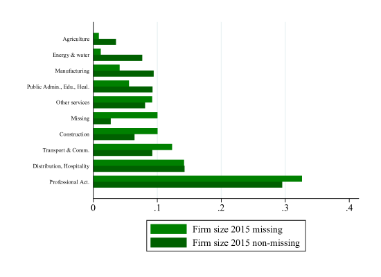
Figure D3: Representativity of FAME sample

Source: FAME, 2015.
Note: This figure compares the industry distribution of FAME firms with missing and non-missing size information in 2015, the year used to to define firms’ treatment status.

Figure D4: Wage posting by industry and occupation

A Occupational distribution

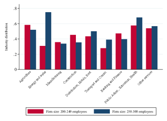
B Industry distribution

Source: BGT, 2015–2017.
Notes: These graphs present the occupational and industry distribution of wage posting, separately for treated and control firms, in the pre-policy period. In each graph, the blue bars refer to the treatment group, firms with 250-300 employees, and the red bars to the control group, firms with 200-249 employees.

Figure D5: Event studies - firms’ hiring practices

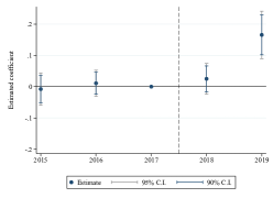
A Wage posting

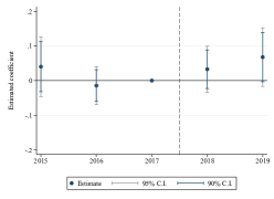
B Log annual wage

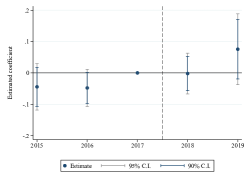
C Wage interval

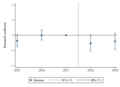
D Interval width

Source: BGT, FAME 2015–2019.
Note: This graph presents the estimates of the leads and lags of the policy on firms’ wage-posting decision and the characteristics of posted wages. These results are obtained from the estimation of the dynamic version of regression 3. The estimation sample includes firms with 200-300 employees, between the financial years 2015 and 2019. The graph also reports 90 and 95 percent confidence intervals associated with firm-level clustered standard errors. The dash vertical line indicates the month when the mandate is approved, i.e., February 2017.

Table D1: Gender equality performance and presence in BGT

	2017/18				2018/19
	Entire	Matched with BGT		P-value	Entire	Matched with BGT		P-value
	sample	Yes	No	difference	sample	Yes	No	difference
	(1)	(2)	(3)	(4)	(5)	(6)	(7)	(8)
Gender pay gap (%)	11.79	12.11	11.31	0.01	11.88	12.26	11.30	0.00
	(15.84)	(15.84)	(15.81)		(15.51)	(15.73)	(15.15)
Women in top quartile (%)	39.20	39.10	39.35	0.60	39.75	39.70	39.84	0.77
	(24.41)	(24.90)	(23.65)		(24.48)	(24.94)	(23.78)
Observations	10,557	6,323	4,234		10,812	6,514	4,298

• Source: BGT 2013–2019, GEO 2018–2019.

• Notes: This table explores potential selection patterns of GEO firms matched with BGT. Column 1 (5) reports the gender median hourly pay gap and percentage of women in the top quartile of the firm wage distribution for all GEO firms in 2017/18 (2018/19); Column 2 (6) refers to firms that match perfectly with a BGT employer; Column 3 (7) refers to firms that do not match perfectly with a BGT employer; Column 4 (8) reports the p-value of the difference in the sample means of these two groups.

• *** p$<$0.01, ** p$<$0.05, * p$<$0.1.

Table D2: FAME firm size and presence in BGT

	Entire	Matched with BGT		P-value
	sample	Yes	No	Difference
	(1)	(2)	(3)
Number of employees	236	231	240	0.05
	(230)	(164)	(286)
Observations	9,771	5,140	4,631

• Source: BGT, FAME, 2013–2019.

• Notes: This table explores potential selection patterns of FAME firms matched with BGT. Column 1 reports the 2015 number of employees of all FAME firms with a number of employees between 200 and 300 in at least one year and non-missing firm size in 2015; Columns 2 and 3 reports the number of employees in 2015 for FAME that do or do not match perfectly with a BGT employer. Finally, Column 4 reports the p-value of the difference in the sample means of these two groups.

Table D3: BGT Summary statistics - pre-policy period

	Treated	Control
	(1)	(2)
Full-time	0.92	0.90
	(0.27)	(0.30)
Observations	25,145	45,563
Full-time vacancies
Higher-paid occupations	0.61	0.56
	(0.49)	(0.50)
Posting wage	0.46	0.45
	(0.50)	(0.50)
Observations	23,211	41,125
Vacancies with wage information
Wage interval	0.51	0.41
	(0.50)	(0.49)
Interval dispersion	1.25	1.23
	(0.23)	(0.20)
Annual wage offered	26,145	29,395
	(14,492)	(19,466)
Observations	10,735	18,400

• Source: BGT, 2015–2017.

• Notes: This table reports mean and standard deviation of the main variables used in the analysis of BGT data, separately for treatment and control groups, before the implementation of the mandate.

Table D4: Impact on wage-posting decision - longer pre-period

	Wage	Log annual	Wage	Interval
	posted	wage	interval	dispersion
	(1)	(2)	(3)	(4)
Panel A: 2015–2019
Treated firm*post	0.043∗	0.040	0.036	-0.046∗
	(0.022)	(0.029)	(0.028)	(0.026)
Observations	97,467	43,752	43,752	19,342
Adjusted $R^{2}$	0.470	0.584	0.414	0.382
Pre-policy mean	0.46	26,116	0.51	1.25
Panel B: 2013–2019
Treated firm*post	0.039∗	0.027	0.016	-0.042∗
	(0.022)	(0.028)	(0.031)	(0.025)
Observations	125,479	56,933	56,933	23,912
Adjusted $R^{2}$	0.474	0.565	0.437	0.378
Pre-policy mean	0.49	26,315	0.44	1.26

• Source: BGT, 2013–2019.

• Notes: This table compares the impact of pay transparency on wage posting and wage characteristics when using the main sample (Panel A) and when including the fiscal years 2013 and 2014. Both sets of results are obtained from the estimation of regression 3. In both panels, the estimation sample comprises BGT firms that have between 200 and 300 employees. In Column 2, it is restricted to vacancies with wage information. In Column 4, it is further restricted to vacancies posting a wage interval. All regressions include firm fixed effects and 5-digit SIC-specific time shocks. A treated firm is defined as having at least 250 employees in 2015. The post dummy is equal to one from the second quarter of 2018 onward. Heteroskedasticity-robust standard errors clustered at firm level in parentheses. The pre-policy mean represents the mean of the outcome variable for the treated group between 2015 (2013) and 2017.

• *** p$<$0.01, ** p$<$0.05, * p$<$0.1.

Table D5: Impact on wage-posting decision - controlling for SOC FE

	Wage	Log annual	Wage	Interval
	posted	wage	interval	dispersion
	(1)	(2)	(3)	(4)
Panel A: Main specification
Treated firm*post	0.043∗	0.040	0.036	-0.046∗
	(0.022)	(0.029)	(0.028)	(0.026)
Observations	97,467	43,752	43,752	19,342
Adjusted $R^{2}$	0.470	0.584	0.414	0.382
Pre-policy mean	0.46	26,116	0.51	1.25
Panel B: Adding 4-digit SOC FE
Treated firm*post	0.044∗∗	0.040	0.038	-0.039
	(0.021)	(0.027)	(0.028)	(0.024)
Observations	97,458	43,725	43,725	19,310
Adjusted $R^{2}$	0.484	0.681	0.429	0.414
Pre-policy mean	0.46	26,116	0.51	1.25

• Source: BGT, 2015–2019.

• Notes: This table compares the impact of pay transparency on wage posting and wage characteristics in the main specification and in a model that controls for 4-digit SOC fixed effects. Both sets of results are obtained from the estimation of regression 3. In both panels, the estimation sample comprises BGT firms that have between 200 and 300 employees. In Column 2, it is restricted to vacancies with wage information. In Column 4, it is further restricted to vacancies posting a wage interval. All regressions include firm fixed effects and 5-digit SIC-specific time shocks. A treated firm is defined as having at least 250 employees in 2015. The post dummy is equal to one from the second quarter of 2018 onward. Heteroskedasticity-robust standard errors clustered at firm level in parentheses. The pre-policy mean represents the mean of the outcome variable for the treated group between 2015 and 2017.

• *** p$<$0.01, ** p$<$0.05, * p$<$0.1.

Table D6: Impact on number of vacancies and occupational distribution

	Log number	SOC1	SOC2	SOC3	SOC4	SOC5	SOC6	SOC7	SOC8	SOC9
	vacancies	share	share	share	share	share	share	share	share	share
	(1)	(2)	(3)	(4)	(5)	(6)	(7)	(8)	(9)	(10)
Treated firm*post	0.028	0.001	0.011	-0.011	-0.005	0.004	-0.001	0.005	-0.002	-0.001
	(0.071)	(0.015)	(0.018)	(0.018)	(0.014)	(0.011)	(0.010)	(0.013)	(0.008)	(0.009)
Observations	11,397	11,397	11,397	11,397	11,397	11,397	11,397	11,397	11,397	11,397
Adjusted $R^{2}$	0.534	0.188	0.392	0.219	0.204	0.380	0.464	0.356	0.477	0.358
Pre-policy mean	1.20	0.12	0.22	0.20	0.11	0.08	0.05	0.12	0.04	0.05

• Source: BGT, 2015–2019.

• Notes: This table reports the impact of pay transparency on firms’ number of vacancies and the occupational distribution of vacancies. The results are obtained from the estimation of regression 3 at firm level. The estimation sample comprises BGT firms that have between 200 and 300 employees. All regressions include firm fixed effects and 5-digit SIC-specific time shocks. A treated firm is defined as having at least 250 employees in 2015. The post dummy is equal to one from the second quarter of 2018 onward. Heteroskedasticity-robust standard errors clustered at firm level in parentheses. The pre-policy mean represents the mean of the outcome variable for the treated group between 2015 and 2017.

• *** p$<$0.01, ** p$<$0.05, * p$<$0.1.

Table D7: Impact on pay outcomes by tenure in the firm

	Entire	$\leq$ 2 years	More than 2 years
	sample	tenure	tenure
	(1)	(2)	(3)
Treated firm*post	-0.026∗∗∗	-0.018	-0.019∗∗
	(0.008)	(0.024)	(0.008)
Treated firm*post*fem	0.029∗∗	0.067	0.017
	(0.014)	(0.045)	(0.015)
Observations	29,226	5,002	21,084
Adjusted $R^{2}$	0.909	0.900	0.916
P-value Women Coeff	0.788	0.198	0.839
P-value High vs. Low M		0.747
P-value High vs. Low W		0.200
Men’s pre-policy mean	15.93	12.59	17.46
Women’s pre-policy mean	13.36	11.37	14.39

• Source: ASHE, 2013–2019.

• Notes: This table compares the impact of pay transparency on employees’ hourly pay across workers with more or at most 2 years of tenure in the firm, by estimating regression 1 by subgroup. Column 1 reports the estimate on log hourly pay for the entire sample, employees working in firms that have between 200 and 300 employees. Columns 2 and 3 compare the impact across tenure groups. All regressions include firm*individual fixed effects, gender*year fixed effects, and region-specific time shocks. A treated firm is defined as having at least 250 employees in 2015. The post dummy is equal to one from 2018 onward. Heteroskedasticity-robust standard errors clustered at firm level in parentheses. The “ P-value Women Coeff” refers to the t-test on the sum of the two reported coefficients, corresponding to the effect of the policy on female employees. The “P-value High vs. Low M (W)” refers to the t-test on the equality of effects on men’s (women’s) pay across tenure groups. The pre-policy mean represents the mean of the outcome variable for the treated group and subgroup considered between 2013 and 2017.

• *** p$<$0.01, ** p$<$0.05, * p$<$0.1.

References

- (1)
- Adams et al. (2020) Adams, Abigail, Maria Balgova, and Qian Matthias, “Flexible Work Arrangements in Low Wage Jobs: Evidence from Job Vacancy Data,” CEPR Discussion Paper No. 15263, Centre for Economic Policy Research 2020.
- Alderman (2018) Alderman, Liz, “Britain Aims to Close Gender Pay Gap with Transparency and Shame,” New York Times, 2018.
- Allcott and Kessler (2019) Allcott, Hunt and Judd B Kessler, “The Welfare Effects of Nudges: A Case Study of Energy Use Social Comparisons,” American Economic Journal: Applied Economics, 2019, 11 (1), pp. 236–276.
- Aumayr-Pintar et al. (2018) Aumayr-Pintar, Christine, Anna-Karin Gustafsson, Anna Savolaine, and Carsten Jørgensen, “Pay Transparency in Europe: First Experiences with Gender Pay Reports and Audits in Four Member States,” Publications Office of the European Union, Luxembourg, 2018.
- Azar et al. (2020a) Azar, José, Ioana Marinescu, and Marshall Steinbaum, “Labor Market Concentration,” Journal of Human Resources, 2020, pp. 1218–9914R1.
- Azar et al. (2020b) , , , and Bledi Taska, “Concentration in US Labor Markets: Evidence from Online Vacancy Data,” Labour Economics, 2020, 66, pp. 101886.
- Azmat et al. (2020) Azmat, Ghazala, Vicente Cuñat, and Emeric Henry, “Gender Promotion Gaps: Career Aspirations and Workplace Discrimination,” Available at SSRN 3518420, 2020.
- Babcock et al. (2003) Babcock, Linda, Sara Laschever, Michele Gelfand, and Deborah Small, “Nice Girls Don’t Ask,” Harvard Business Review, 2003, 81 (10), pp. 14–16.
- Baker et al. (2022) Baker, Michael, Yosh Halberstam, Kory Kroft, Alexandre Mas, and Derek Messacar, “Pay Transparency and the Gender Gap,” American Economic Journal: Economic Policy, 2022, Forthcoming.
- Banfi and Villena-Roldan (2019) Banfi, Stefano and Benjamin Villena-Roldan, “Do High-wage Jobs Attract More Applicants? Directed Search Evidence from the Online Labor Market,” Journal of Labor Economics, 2019, 37 (3), pp. 715–746.
- Belot et al. (2022) Belot, Michèle, Philipp Kircher, and Paul Muller, “How Wage Announcements Affect Job Search – A Field Experiment,” American Economic Journal: Macroeconomics, 2022, 14 (4), pp. 1–67.
- Bennedsen et al. (2021) Bennedsen, Morten, Elena Simintzi, Margarita Tsoutsoura, and Daniel Wolfenzon, “Do Firms Respond to Gender Pay Gap Transparency?,” Journal of Finance, forthcoming, 2021.
- Bertrand (2020) Bertrand, Marianne, “Gender in the Twenty-first Century,” in “AEA Papers and proceedings,” Vol. 110 2020, pp. 1–24.
- Biasi and Sarsons (2022) Biasi, Barbara and Heather Sarsons, “Flexible Wages, Bargaining, and the Gender Gap,” The Quarterly Journal of Economics, 2022, 137 (1), pp. 215–266.
- Bowles et al. (2007) Bowles, Hannah Riley, Linda Babcock, and Lei Lai, “Social Incentives for Gender Differences in the Propensity to Initiate Negotiations: Sometimes it Does Hurt to Ask,” Organizational Behavior and human decision Processes, 2007, 103 (1), pp. 84–103.
- Breza et al. (2018) Breza, Emily, Supreet Kaur, and Yogita Shamdasani, “The Morale Effects of Pay Inequality,” The Quarterly Journal of Economics, 2018, 133 (2), pp. 611–663.
- Burn and Kettler (2019) Burn, Ian and Kyle Kettler, “The More You Know, the Better You’re Paid? Evidence from Pay Secrecy Bans for Managers,” Labour Economics, 2019, 59, pp. 92–109.
- Card et al. (2012) Card, David, Alexandre Mas, Enrico Moretti, and Emmanuel Saez, “Inequality at Work: the Effect of Peer Salaries on Job Satisfaction,” American Economic Review, 2012, 102 (6), pp. 2981–3003.
- Card et al. (2016) , Ana Rute Cardoso, and Patrick Kline, “Bargaining, Sorting, and the Gender Wage Gap: Quantifying the Impact of Firms on the Relative Pay of Women,” The Quarterly journal of economics, 2016, 131 (2), pp. 633–686.
- Chu (2018) Chu, Ben, “Company Gender Pay Gap Reporting Is Already Helping, and Will Continue to Help Tackle Inequalities,” The Independent, 2018.
- Cullen and Pakzad-Hurson (2021) Cullen, Zoë and Bobak Pakzad-Hurson, “Equilibrium Effects of Pay Transparency,” NBER Working Paper No. 28903, National Bureau of Economic Research 2021.
- Cullen and Perez-Truglia (2018) and Ricardo Perez-Truglia, “The Salary Taboo: Privacy Norms and the Diffusion of Information,” NBER Working Paper No. 25145, National Bureau of Economic Research 2018.
- Cullen and Perez-Truglia (2021) and , “How Much Does Your Boss Make? The Effects of Salary Comparisons,” Journal of Political Economy, forthcoming, 2021.
- Dahlgreen et al. (2018) Dahlgreen, Will, Ransome Mpini, Daniele Palumbo, and Clara Guibourg, “What is the Gender Pay Gap at Your Company?,” BBC News, 2018.
- Deming and Kahn (2018) Deming, David and Lisa B Kahn, “Skill Requirements across Firms and Labor Markets: Evidence from Job Postings for Professionals,” Journal of Labor Economics, 2018, 36 (S1), pp. S337–S369.
- Downing et al. (2015) Downing, Christabel, Erica Garnett, Katie Spreadbury, and Mark Winterbotham, “Company Reporting: Gender Pay Data,” Technical Report, IFF Research 2015.
- Dube et al. (2019) Dube, Arindrajit, Laura Giuliano, and Jonathan Leonard, “Fairness and Frictions: the Impact of Unequal Raises on Quit Behavior,” American Economic Review, 2019, 109 (2), pp. 620–63.
- Elsby and Solon (2019) Elsby, Michael WL and Gary Solon, “How Prevalent is Downward Rigidity in Nominal Wages? International Evidence from Payroll Records and Pay Slips,” Journal of Economic Perspectives, 2019, 33 (3), pp. 185–201.
- Flinn and Mullins (2021) Flinn, Christopher and Joseph Mullins, “Firms’ Choices of Wage-Setting Protocols,” Technical Report, Discussion paper, New York University 2021.
- Giuliano (2021) Giuliano, Paola, “Gender and Culture,” Oxford Review of Economic Policy, 2021, 36 (4), pp. 944–961.
- Government Equalities Office (2015) Government Equalities Office, GEO, “Closing the Gender Pay Gap. Government Consultations,” Technical Report 2015.
- Gulyas et al. (2022) Gulyas, Andreas, Sebastian Seitz, and Sourav Sinha, “Does Pay Transparency Affect the Gender Wage Gap? Evidence from Austria,” American Economic Journal: Economic Policy, 2022, Forthcoming.
- Hall and Krueger (2012) Hall, Robert E and Alan B Krueger, “Evidence on the Incidence of Wage Posting, Wage Bargaining, and On-the-job Search,” American Economic Journal: Macroeconomics, 2012, 4 (4), pp. 56–67.
- Johnson (2020) Johnson, Matthew S, “Regulation by Shaming: Deterrence Effects of Publicizing Violations of Workplace Safety and Health Laws,” American Economic Review, 2020, 110 (6), pp. 1866–1904.
- Kommenda et al. (2018) Kommenda, Niko, Caelainn Barr, and Josh Holder, “Gender Pay Gap: What We Learned and How to Fix It,” The Guardian, 2018.
- Kuhn and Shen (2013) Kuhn, Peter and Kailing Shen, “Gender Discrimination in Job Ads: Evidence from China,” The Quarterly Journal of Economics, 2013, 128 (1), pp. 287–336.
- Leibbrandt and List (2015) Leibbrandt, Andreas and John A List, “Do Women Avoid Salary Negotiations? Evidence from a Large-Scale Natural Field Experiment,” Management Science, 2015, 61 (9), pp. 2016–2024.
- Luca (2018) Luca, Dara Lee, “The Digital Scarlet Letter: The Effect of Online Criminal Records on Crime,” Available at SSRN 1939589, 2018.
- Marinescu and Wolthoff (2020) Marinescu, Ioana and Ronald Wolthoff, “Opening the Black Box of the Matching Function: the Power of Words,” Journal of Labor Economics, 2020, 38 (2), 535–568.
- Martin (2020) Martin, Josh, “Homeworking Hours, Rewards and Opportunities in the UK: 2011 to 2020,” ONS, 2020.
- Mas (2017) Mas, Alexandre, “Does Transparency Lead to Pay Compression?,” Journal of Political Economy, 2017, 125 (5), pp. 1683–1721.
- Pedregosa et al. (2011) Pedregosa, F., G. Varoquaux, A. Gramfort, V. Michel, B. Thirion, O. Grisel, M. Blondel, P. Prettenhofer, R. Weiss, V. Dubourg, J. Vanderplas, A. Passos, D. Cournapeau, M. Brucher, M. Perrot, and E. Duchesnay, “Scikit-learn: Machine Learning in Python,” Journal of Machine Learning Research, 2011, 12, 2825–2830.
- Perez-Truglia and Troiano (2015) Perez-Truglia, Ricardo and Ugo Troiano, “Shaming Tax Delinquents: Theory and Evidence from a Field Experiment in the United States,” Citeseer, 2015.
- Roussille (2020) Roussille, Nina, “The Central Role of the Ask Gap in Gender Pay Inequality,” Working Paper, 2020.
- Ruddick (2018) Ruddick, Graham, “Women at BBC Criticise Pay Review over Failure to Identify Gender Bias,” The Guardian, 2018.
- Siniscalco et al. (2017) Siniscalco, Gary R, Erin M Connell, and Chad Smith, “State Pay Equity Laws: Where a Few Go, Many May Follow,” Technical Report, Mimeo 2017.
- Sran et al. (2020) Sran, Gurpal, Felix Vetter, and Matthew Walsh, “Employer Responses to Pay History Inquiry Bans,” Available at SSRN 3587736, 2020.
- Strauss (2019) Strauss, Delphine, “Gender Pay Reporting: Does it Make a Difference?,” Financial Times, 2019.
- Wisniewska et al. (2018) Wisniewska, Aleksandra, Billy Ehrenberg-Shannon, and Sarah Gordon, “Gender Pay Gap: How Women are Short-Changed in the UK,” Financial Times, 2018.
- Wright et al. (2021) Wright, Randall, Philipp Kircher, Benoît Julien, and Veronica Guerrieri, “Directed Search and Competitive Search Equilibrium: A Guided Tour,” Journal of Economic Literature, 2021, 59 (1), pp. 90–148.