SOCIAL NETWORKS AS A MECHANISM FOR DISCRIMINATION

I study labor markets in which firms hire via referrals. I develop an employment model showing that—despite initial equality in ability, employment, wages, and network structure—minorities receive fewer jobs through referral and lower expected wages, simply because their social group is smaller. This disparity, termed “social network discrimination,” falls outside the dominant economics discrimination models—taste-based and statistical. Social network discrimination can be mitigated by minorities having more social ties or a “stronger-knit” network. I calibrate the model using a nationally-representative U.S. sample and estimate the lower-bound welfare gap caused by social network discrimination at over four percent, disadvantaging black workers.

Keywords: discrimination, diversity, employment, homophily, inequality, labor market, social networks

JEL Codes: D63, D85, J31, J71, Z13

1 Introduction

In the U.S. context, the vestiges of slavery and state-enforced racial segregation directly and indirectly have contributed to racial disparities, confounding efforts to foster equality. Suppose, however, that the circumstances of racial groups were equalized—that the slate was wiped clean. In a world without prejudice—and one beginning in a state of equality—would labor market disparities still arise between majority and minority workers?

In this paper, I develop an employment model and assume equal ability, employment, and network structure between majority and minority workers in the initial time period. Despite these equalizing assumptions, I find that if majority and minority workers have (1) an equal chance of having a social tie (i.e., an equivalent network density) and (2) an equal bias in favor of forming same-group social ties (i.e., an equivalent type in-group bias), then the probability of a firm offering a job through referral to minority workers is lower than their share of the labor force. For minority workers to have a proportional chance of receiving job offers through referral, they must compensate with a stronger network density and/or type in-group bias. The estimated welfare gap increases in a convex way with the majority group share of the labor force, suggesting that the disadvantage of minority workers magnifies with the degree of their minority status in the labor market. Finally, this paper calibrates the model, estimating the lower bound welfare gap between black and white workers caused by social network discrimination.

While the model may work for arbitrary assignments of majority and minority groups, social science research suggests that race and ethnicity create the greatest divide socially [29]. Hence, this paper’s findings impact debates surrounding the merits of race-conscious policies. Many who are critical of such policies share a common assumption: that in a world without historical discrimination—without Jim Crow or implicit biases—“no policy” would be the best policy. No policy would yield the most meritocratic outcome, with opportunities distributed according to corresponding ability or “merit.” Yet the findings in this paper suggest otherwise. Achieving equality of opportunity may remain elusive even in the absence of psychological prejudice, historical wrongs, and differences in ability or education among racial groups. Advantages from being within a larger or more strongly-connected social network may persist, despite one’s talent. All else equal, outcomes may remain unequal.

This paper makes four contributions. First, the paper presents a novel theoretical approach for uncovering discriminatory outcomes independent from discriminatory motives (i.e., independent from both prevailing models of discrimination in economics: taste-based and statistical)—these discriminatory outcomes arise even under an initial state of equality between majority and minority groups, unlike in previous work. In other words, not only does this paper develop a standard labor-market model that reveals the limitations of past economic models of discrimination, but also this work offers a direct rigorous account of what I term “social network discrimination” using mainstream economic theory. Second, this paper performs equilibrium analysis of employment and wage differences caused by homophily along majority/minority status, which is a contribution to both the economic and sociological literatures on labor markets. Third, in doing so the paper isolates a potential underlying mechanism for inequality, adding to our understanding of racial disparities that have been widely studied across the social sciences. The paper accomplishes this while making predictions on when disparities might arise—as well as on when they might not. Fourth, the paper calibrates the model using a nationally-representative sample from the National Longitudinal Study of Adolescent to Adult Health. In this calibration exercise, white respondents represent the majority group and black respondents represent the minority group. Through calibration, I estimate that the lower bound welfare gap—i.e., the difference in expected wages—caused by social network discrimination is over four percent, with black respondents disadvantaged compared to white ones. To the best knowledge of the author, there has not been any prior quantification of the magnitude of the impact social network discrimination has in isolation on racial disparities.

Contributions to Literature— The model in this paper extends the one from [31] to incorporate two-dimensional heterogeneity: while the original model only groups workers by ability, this paper also groups them by majority/minority status. Doing so yields findings that go far beyond a mere application of the base model. The original model does not focus on outcomes when homophily (the well-documented tendency for people to associate more with others similar to themselves) exists along characteristics uncorrelated with ability—namely, on what effects emerge when social ties are formed along dimensions orthogonal to productivity. The original model does not incorporate demographic considerations.

Filling this gap is important. Within sociology, research has explored homophily in various contexts, including its causes [43, 27] as well as how it influences friendships [7, 42], interethnic marriages [40], and social inequality [18], among other areas. Within economics, there is an extant literature on the impact of referrals on inequality, yet many findings have relied on the existence of some degree of prior period inequality beyond majority/minority group size—for example, that if a demographic group has higher past employment, then that would yield an advantage in securing future jobs. This paper adds to insights from both fields, demonstrating that referral advantages may still unequally accrue over time even under initial equality between majority/minority groups, due to homophily. In particular, this paper adds a theoretical foundation for why homophily may contribute to inequality in referral markets, as well as predicts under what conditions such disparities will not surface.

There has been increasing focus on uncovering mechanisms behind racial disparities in labor market outcomes [4, 17] and wage inequalities [15, 26]. Evidence for racial differences in networking outcomes exists [24, 25, 30, 28]. [23] discusses how homophily leads to segregation of groups, which leads to different equilibrium investment decisions in areas like education. Yet this paper introduces a more direct mechanism for inequality from homophily: that even given equal investments in human capital, homophily may still directly foster disparities through hiring dynamics. [8] finds that inequality due to homophily arises as a function of historical employment, whereas this paper does not rely on historical differences in labor market conditions. Similarly, unlike in [14], which provides a network-based mechanism for inequality deriving from differential drop-out rates, this paper uncovers how homophily can lead to inequality through the channel of employment opportunities themselves. Thus, this paper introduces a direct mechanism through which homophily can generate inequality that does not rely on historical differences between social groups, a contribution not previously found in the literature to the best knowledge of the author. In addition, this paper’s findings add to ones from sociology that link homophily to social inequality [18, see, e.g.,]; in this paper, in contrast, homophily’s impact on inequality does not operate through a mechanism that exacerbates individual level differences (recall our model assumes groups have equal ability and initial employment). Notably, this paper’s findings are also distinct from past economics and sociology research on the influence of more traditional discrimination in hiring [6, 33, see, e.g.,]. Unlike those articles, this one uncovers disparities even in contexts in which discriminatory motives and implicit biases are not only absent but impossible, as the model in this paper does not allow firms to distinguish who is a majority and who is a minority worker. Significantly, if the biases suggested by such prior research are incorporated—biases which tend to favor the majority group—the size of the disparities predicted in this paper’s model would be even larger.

This paper proceeds as follows: Section 2 introduces a formal setup of the model. Section 3 presents the model’s key findings for majority and minority workers. Section 4 provides discussion. Section 5 performs a calibration of the model under simplifying assumptions. Section 6 concludes.

2 Model

Here, I extend the [31] two-period model to incorporate two-dimensional heterogeneity: while the original model only groups workers by ability, this one also groups them by majority/minority status.

Workers: I consider a labor market with two time periods ($t=1$ and $t=2$) and many workers, with an equal measure in each period. Each worker works one period, and is one of two types: majority or minority. Each worker’s type is predetermined and assigned before the period in which he or she enters the market. The fraction of majority workers is $\delta>\frac{1}{2}$, while $1-\delta<\frac{1}{2}$ are minority. Similar to [31], I assume that $\frac{1}{2}$ of the workers within each type are high-ability, while $\frac{1}{2}$ are low-ability. High-ability workers produce one unit of output, while low-ability workers produce zero units. Workers are observationally equivalent: firms neither know what ability workers possess (before production), nor whether workers are of the majority or minority type (at any time).

Firms: Firms are free to enter the market in either period. At most, each firm may employ one worker. A firm’s profit in each period is equal to the productivity of its worker minus the wage paid. Each firm must set wages before it learns the productivity of its worker. There are no output-contingent contracts.

Structure of Social Network: As the focus of the model is referrals, now I describe how the social network through which referrals occur is drawn. As described, there are four categories of workers: high-ability majority, high-ability minority, low-ability majority, and low-ability minority. Now let us represent each period-2 worker as an urn, and each social tie that a period-1 worker possesses as a ball. The assignment of social ties is equivalent to a scenario where the balls are randomly dropped into the urns. A period-1 worker possesses a social tie (“ball”) with a probability equal to its majority/minority type’s network density (denoted by $\tau_{maj}$ or $\tau_{min}$). A period-1 worker’s sole social tie, if they have one, is dropped into an “urn” (period-2 worker) which is: (1) of the same ability with probability $\alpha\in(\frac{1}{2},1)$; and (2) of the same majority/minority type with a probability determined by the period-1 worker’s in-group bias. The network structure is thus characterized by three parameters: network density ($\tau_{maj}$ and $\tau_{min}$), majority/minority type in-group bias (denoted by $\psi_{maj}$ and $\psi_{min}$, respectively), and ability in-group bias ($\alpha$).

Timing: Each firm hires a period-1 worker through the market and learns his or her ability. As period-1 workers are observationally equivalent (and cannot be referred for jobs since there is no previous time period), each firm hiring through the market receives a high-ability worker with probability $\frac{1}{2}$.

After learning the ability of its current worker, each firm may set a referral offer to be relayed to the worker’s social tie. Whether the referral offer is relayed is conditional on the firm’s worker holding a social tie. If he or she does hold one, then the firm will only attract the acquaintance if the referral offer exceeds both the period-2 market wage and all other referral offers received by the acquaintance. A firm not wishing to hire through referral will set no referral offer (or might just set a referral offer below the period-2 market wage, which has no probability of acceptance). Period-2 workers then compare all offers received, accepting the highest.

All period-2 workers who receive no referral offers must find employment through the general market.

In summary, the timing of the game is as follows.

1. Each firm hires period-1 workers through the market at a wage of $w_{M1}$.

2. Period-1 production occurs, after which each firm learns the productivity of its worker.

3. Social ties are determined.

4. If a firm wishes to hire through referral, it sets a referral offer. I denote firm $i$’s referral offer by $w_{Ri}$. (Conditional on having a social tie, each period-1 worker then relays his or her firm’s wage offer ($w_{Ri}$) to their period-2 acquaintance.)

5. Each period-2 worker compares all wage offers received. They either accept one or wait to find employment through the general market.

6. Any period-2 worker with no offers (or who refuses all offers) goes on the market. Wages in this market are denoted $w_{M2}$.

7. Period 2 production occurs.

2.1 Note on In-Group Bias

The “in-group bias” can be conceptualized as capturing the fact that there are shared attributes that simply make it easier for some workers to form social ties with each other than with others. For example, for a given chance encounter, one is more likely to form a social tie with another worker who shares a more similar background, because there are simply more elements in common to establish the foundation of a relationship. Hence, “in-group bias” does not represent favoritism toward a demographic group: in the model, any given worker views members of one’s own majority/minority group and members of the other group equivalently, conditional on having a social tie. Similarly, conditional on not having a social tie, any given worker views members of the same majority/minority group and members of the other group with the same level of (dis)interest. Hence, although “in-group bias” deeply impacts network formation, it is fully distinct from (racial or group) animus, in-group favoritism, or traditional conceptions of taste-based preferences.

Figure I: Model Parameters

Parameter	Name	Description	Range
$\delta$	Majority share	Share of the total labor force comprised of majority workers	$\delta\in(\frac{1}{2},1)$
$1-\delta$	Minority share	Share of the total labor force comprised of minority workers	$1-\delta\in(0,\frac{1}{2})$
$\alpha$	Ability in-group bias	Probability a worker’s social tie is with another worker of equal ability	$\alpha\in(\frac{1}{2},1)$
$\tau_{maj}$	Network density (majority group)	Probability a majority worker has a social tie	$\tau_{maj}\in(0,1)$
$\tau_{min}$	Network density (minority group)	Probability a minority worker has a social tie	$\tau_{min}\in(0,1)$
$\psi_{maj}$	Type in-group bias (majority group)	Bias a majority worker exhibits toward workers of the same group in favor of forming social ties. Value of 1/2 means no bias (probability of social tie with another majority worker = $\delta$). Value of 1 means full bias (probability of social tie with another majority worker = 1).* I assume neither full nor no bias.	$\psi_{maj}\in(\frac{1}{2},1)$
$\psi_{min}$	Type in-group bias (minority group)	Bias a minority worker exhibits toward workers of the same group in favor of forming social ties. Value of 1/2 means no bias (probability of social tie with another minority worker = $1-\delta$). Value of 1 means full bias (probability of social tie with another minority worker = 1).* I assume neither full nor no bias.	$\psi_{min}\in(\frac{1}{2},1)$

*$\psi\in[0,\frac{1}{2})$ represents heterophily, a rare social network phenomenon outside the scope of this paper.

3 Equilibrium

I examine a competitive equilibrium of the economy in which firms seek to maximize profits.

The first subsection below presents basic equilibrium properties shared with [31]. The second subsection presents new propositions that I have added to the model by incorporating two-dimensional heterogeneiy (i.e., categorization of workers by majority and minority type in addition to (instead of solely by) ability level). These new propositions relate to discrimination and labor market disparities.

3.1 Basic Equilibrium Properties

Basic equilibrium properties can be expressed via the following three lemmas, which establish that (1) referral wage offers are dispersed within an interval between the period-2 market wage and a maximum referral wage offer; (2) a firm will only hire through referral if it employs a high-ability worker in period 1; and (3) the period-1 market wage is greater than the expected period-1 productivity. More discussion on each of these points is included below. Omitted proofs are found in the Appendix.

Lemma 1

Referral wage offers lie within the interval between $w_{M2}$ and a maximum referral wage offer $\overline{w}_{R}$; hence, $w_{R}\in[w_{M2}$, $\overline{w}_{R}$]. The density of the referral wage offer distribution is positive across this entire range.

Proof. Claim 4 in [10] establishes the existence and uniqueness of an equilibrium, while Theorem 4 proves wage dispersion exists in the equilibrium (since the probability that a period-2 worker receives exactly one referral offer is strictly between 0 and 1). Given this wage dispersion, the market wage ($w_{M2}$) must coincide with the bottom of the referral wage distribution, as any referral offer below the market wage will necessarily be rejected by workers in favor of going to the general market. At the maximum referral wage offer (denoted $\overline{w}_{R}$ and derived in Appendix Equation A.7), the probability a worker accepts the referral offer is 1. Hence, firms will not offer a referral wage above this amount as it will necessarily reduce profits. Proposition 2.2 in [12] proves that there are no gaps in the wage distribution. If there were a gap between some $w_{1}$ and $w_{2}$, then a firm offering the higher wage could reduce its offer by $\epsilon$ without reducing the probability its offer is accepted, thereby increasing its profits.   

Lemma 2

A firm will attempt to hire through referral if and only if it employs a high-ability worker in period 1.

This result follows from the ability in-group bias ($\alpha$). Hiring through the market yields zero expected profit (due to the free entry of firms and the symmetric lack of information on the ability of workers). For firms employing high-ability workers in period 1, an accepted referral offer yields constant positive profit over the range of the referral offer distribution $[w_{M2},\overline{w}_{R}]$. Higher wage offers yield a higher probability of attracting a period-2 worker. Firms employing low-ability workers in period 1 will not hire through the referral market, since the ability in-group bias means the referred worker will more likely also be low-ability.

As a result of this lemma, a disproportionately high number of low-ability workers find employment through the general market. This drives the market wage below the average productivity of the entire population. However, adverse selection does not eliminate the market. Since some high-ability workers are not “well-connected,” they fail to receive referral wage offers, which leads them to find employment in the general market. Thus, the market wage remains above zero.

Lemma 3

The period-1 market wage is greater than the expected period-1 productivity.

If a firm obtains a high-ability worker in period 1, they expect positive period-2 profits. This fact drives the period-1 market wage higher than the productivity of the population. This wage can be viewed as comprising the average productivity of the worker plus an “option value” of a period-2 referral. This option will be exercised if the period-1 worker reveals themselves to be high-ability (which occurs after period-1 production concludes, if the worker is in fact high-ability).

3.2 Propositions on Social Network Discrimination

New propositions reflecting social network discrimination and inequality are detailed below. The propositions establish that minority workers receive a disproportionately low fraction of job offers through referral and a lower expected wage, all else equal. Recall that the market wage lies below the referral offer distribution. Hence, all these effects taken together yield a welfare gap between minority and majority workers in period 2 that did not exist in period 1. Omitted proofs are in the Appendix.

Proposition 1A

In an environment with equal magnitude of majority/minority network parameters ($\tau_{maj}=\tau_{min}$ and $\psi_{maj}=\psi_{min}$), the probability a high-ability minority worker in period 2 receives a referral offer is lower than their share of the labor force. The inverse holds for majority workers:

$$\Pr\{\text{period-2 high-ability minority worker receives referral offer}\}<\frac{1-\delta}{2}$$

$$\Pr\{\text{period-2 high-ability majority worker receives referral offer}\}>\frac{\delta}{2}$$

Proposition 1B

The inequality in the distribution of referral job offers can be eliminated by minority workers having a sufficiently higher type in-group bias ($\psi_{min}$).

Simplified Numerical Example:

First I explore the intuition of Proposition 1A by using a simple numerical example that illustrates type in-group bias. Suppose there are two majority workers in both periods, and one minority worker in both periods—i.e., $\delta=2/3$. Also suppose there is type in-group bias: each worker has a bias in favor of forming social ties with workers of the same majority/minority type. To illustrate this bias, let us say that for encounters between majority period-1 and majority period-2 workers, there is a 2/3 chance of forming a tie, whereas encounters between a majority period-1 and minority period-2 worker has a 1/3 chance of forming a tie—i.e., $\psi=2/3$. Suppose all three period-1 workers encounter all three period-2 workers. The expected number of ties period-1 majority workers form with their own type is thus 4/3 (while the expected number of ties with minority workers is 1/3); this means the fraction of same-type social ties for majority workers is 4/5. Let $\phi_{maj}=0.8$ denote this fraction of same-type social ties (note that $\phi$ is not a parameter of the model and can be calculated directly from $\psi$ via Equation 1 below). Similarly, it is straightforward to calculate that the fraction of same-type social ties for the period-1 minority worker is $\phi_{min}=0.5$.

Now let us apply these bias dynamics to a case in which period-1 workers each have exactly one social tie with probability 1 (i.e., $\tau_{maj}=\tau_{min}=1$). The fraction of referral job offers going to majority workers is simply a weighted sum:

$$\Pr\{\text{referral job offer goes to majority per-2 worker}\}$$

$$=\Pr\{\text{per-1 worker is majority}\}\cdot\Pr\{\text{per-1 majority knows per-2 majority}\}$$

$$\qquad+\Pr\{\text{per-1 worker is minority}\}\cdot\Pr\{\text{per-1 minority knows per-2 majority}\}$$

$$=\delta\cdot\tau_{maj}\cdot\phi_{maj}+(1-\delta)\cdot\tau_{min}\cdot(1-\phi_{min})$$

$$=2/3\cdot 1\cdot 0.8+1/3\cdot 1\cdot 0.5$$

$$=0.7$$

Hence, only 0.3 of referral job offers go to minority workers, even though they occupy 1/3 of the labor force. This simple example illustrates the distorting influence of having the same magnitude of bias operating on groups of different sizes. The bias in favor of a same-group social tie for a majority worker extends toward a greater fraction of the population than does the same magnitude of bias for a minority worker. Hence, equal magnitudes of bias unequally impact the respective chances of knowing workers of the same type. [End of Example]

I can generalize both the reasoning of the simplified numerical example above and the type-in group bias of the model as follows:

(1) $$\Pr\{\text{period-1 worker knows own maj/min type}\}=\phi=\frac{w\cdot\psi}{[w\cdot\psi]+[(1-w)(1-\psi)]}$$

where $w$ is the share of the labor force for the worker type (either $\delta$ or $1-\delta$) and $\psi$ is the in-group bias of the worker type (either $\psi_{maj}$ or $\psi_{min}$). $\psi=0.5$ reflects no bias—i.e., a proportional chance of a social tie being with another of the same type—and $\psi=1$ reflects when all ties are with members of the same type. $\phi$ represents either $\phi_{maj}$ or $\phi_{min}$, depending on whether the period-1 worker belongs to the majority or minority group, respectively. The Discussion section further explores the relationship between $\psi$ and $\phi$, and its implications on the results.

In the Appendix, I prove that parity in the distribution of job offers between high-ability majority and minority workers is accomplished only when:

(2) $$(1-\delta)\left[\delta\tau_{maj}\phi_{maj}+(1-\delta)\tau_{min}(1-\phi_{min})\right]=\delta\left[\delta\tau_{maj}(1-\phi_{maj})+(1-\delta)\tau_{min}(\phi_{min})\right]$$

where $\phi_{maj}$ and $\phi_{min}$ are calculated from Equation 1 above. From Equation 2, one can calculate what magnitude other parameters must be for parity. I denote such parameters for minority workers as $\tau_{min}^{=}$ (compensating network density) and $\psi_{min}^{=}$ (compensating in-group bias). Figure II illustrates that a sufficiently high network density or type in-group bias can mitigate the disproportionality in the distribution of job offers through referral. All else equal, minority workers can either have more social ties ($\tau_{min}^{=}>\tau_{maj}$) or a “stronger-knit” social network ($\psi_{min}^{=}>\psi_{maj}$).

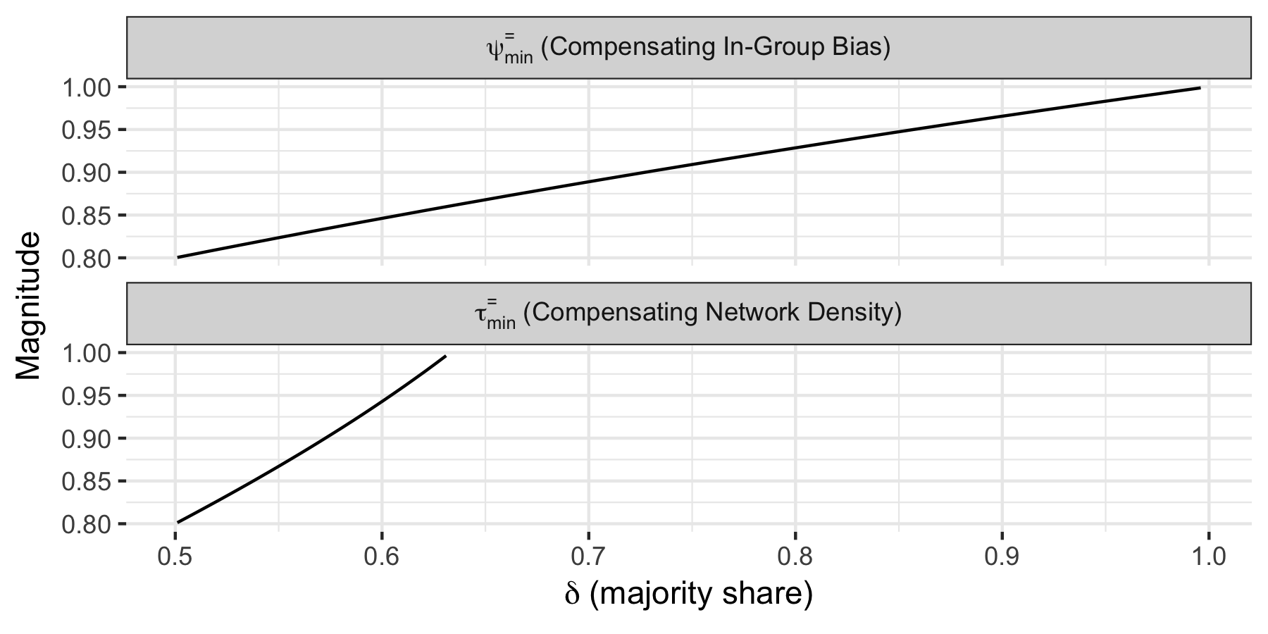
Figure II: Magnitude of Minority Group Network Parameters
Required for Parity in Referral Job Offers^*

^*In each chart, all other relevant network parameters = 0.8.

The network density required to eliminate the inequality ($\tau_{min}^{=}$) increases in $\tau_{maj}$, $\psi_{maj}$, and $\delta$. It decreases in $\psi_{min}$, which can readily be understood intuitively. The greater the probability of majority workers having social ties (and/or the greater the degree of their homophily), the greater minority workers’ compensating parameters ($\tau_{min}^{=}$ or $\psi_{min}^{=}$) must be to achieve a proportional amount of all job offers through referrals. In Figure II, the plot of $\tau_{min}^{=}$ has no values when $\delta$ is greater than approximately 0.63. This is because there is no attainable magnitude of network density that will yield parity in the distribution of job offers when $\delta$ surpasses this threshold.

Proposition 2

In an environment with equal magnitude of majority/minority network parameters ($\tau_{maj}=\tau_{min}$ and $\psi_{maj}=\psi_{min}$), the period-2 market wage ($w_{M2}$) decreases as majority workers occupy a greater fraction of the labor force. $w_{M2}$ also decreases in the ability in-group bias $\alpha$.

Recall that workers who do not receive jobs through referral must find employment through the market. Proposition 1 shows that minority workers, all else equal, receive a disproportionately low fraction of job offers through referral, and thus disproportionately find employment through the market. Decreases in the market wage ($w_{M2}$) thereby hurt the average welfare of minority workers, relative to that of majority workers.

The Appendix includes the expression for $w_{M2}$. Given $\alpha>\frac{1}{2}$, $w_{M2}$ is always less than $\frac{1}{2}$, the average productivity of the population. Analysis shows that $w_{M2}$ is decreasing in $\alpha$. For all $\psi_{maj}=\psi_{min}$ and $\tau_{maj}=\tau_{min}$, $w_{M2}$ also decreases in $\delta$.

Proposition 3

In an environment with equal magnitude of majority/minority network parameters ($\tau_{maj}=\tau_{min}$ and $\psi_{maj}=\psi_{min}$), the referral wage and welfare (i.e., average expected wage) for minority workers is lower than for majority workers.

Much of the intuition behind this finding follows from Proposition 1 (that majority workers receive a disproportionately high number of job offers through referral). There are two margins to consider. First, the extensive margin: majority workers disproportionately get hired through the referral market (which provides higher wages than the general market), driving up expected welfare for the majority group. Second, the intensive margin: recall that workers accept the maximum referral wage offer received. Hence, by majority workers receiving a higher number of referral offers, their expected maximum offer increases, thereby also driving up their relative welfare.

Let $E\prod_{H}(w_{R})$ denote the expected period-2 profit earned by a firm employing a high-ability worker and setting a referral wage. To maintain equilibrium wage dispersion, firms must earn the same expected profit on each referral wage offered:

$$E\prod_{H}(w_{R})=c\qquad\forall w_{R}\in[w_{M2},\overline{w}_{R}]$$

Given the expression for $c$ derived in the Appendix, firms with high-ability workers who have social ties earn positive expected profits as long as $\alpha>\frac{1}{2}$. Analysis shows that $c$ is increasing in $\tau_{maj}$ and $\tau_{min}$. Furthermore, the equilibrium referral-offer distribution $F(\bullet)$ may be determined by setting $E\prod_{H}(w_{R})$ equal to $c$ for all potential wage offers $w_{R}$.

Unfortunately, doing so does not yield a closed-form solution for $F(w_{R})$. Given a continuum of firms, the equilibrium referral-offer distribution $F(\bullet)$ can be interpreted as either: 1) each firm randomizes over the entire distribution; or 2) a fraction $f(w_{R})$ of firms offers each wage for sure. From the second interpretation, I denote these referral wages with $w_{Rk}$. One can then derive an expression for $w_{Rk}(\alpha,\delta,\tau_{maj},\tau_{min},\psi_{maj},\psi_{min},F(w_{Rk}))$ and calculate an average referral wage received by a majority worker (denoted $E(w_{R_{Hmaj}})$) vs. a minority worker (denoted $E(w_{R_{Hmin}})$), for any given $\delta$, $\alpha$, $\tau_{maj}$, $\tau_{min}$, $\psi_{maj}$, and $\psi_{min}$.

Analysis shows that when majority/minority network parameters are the same magnitude, if $\alpha>\frac{1}{2}$ and $\delta>\frac{1}{2}$, $E(w_{R_{Hmaj}})>E(w_{R_{Hmin}})$. In other words, the expected referral wage for high-ability majority workers is greater than for high-ability minority workers.

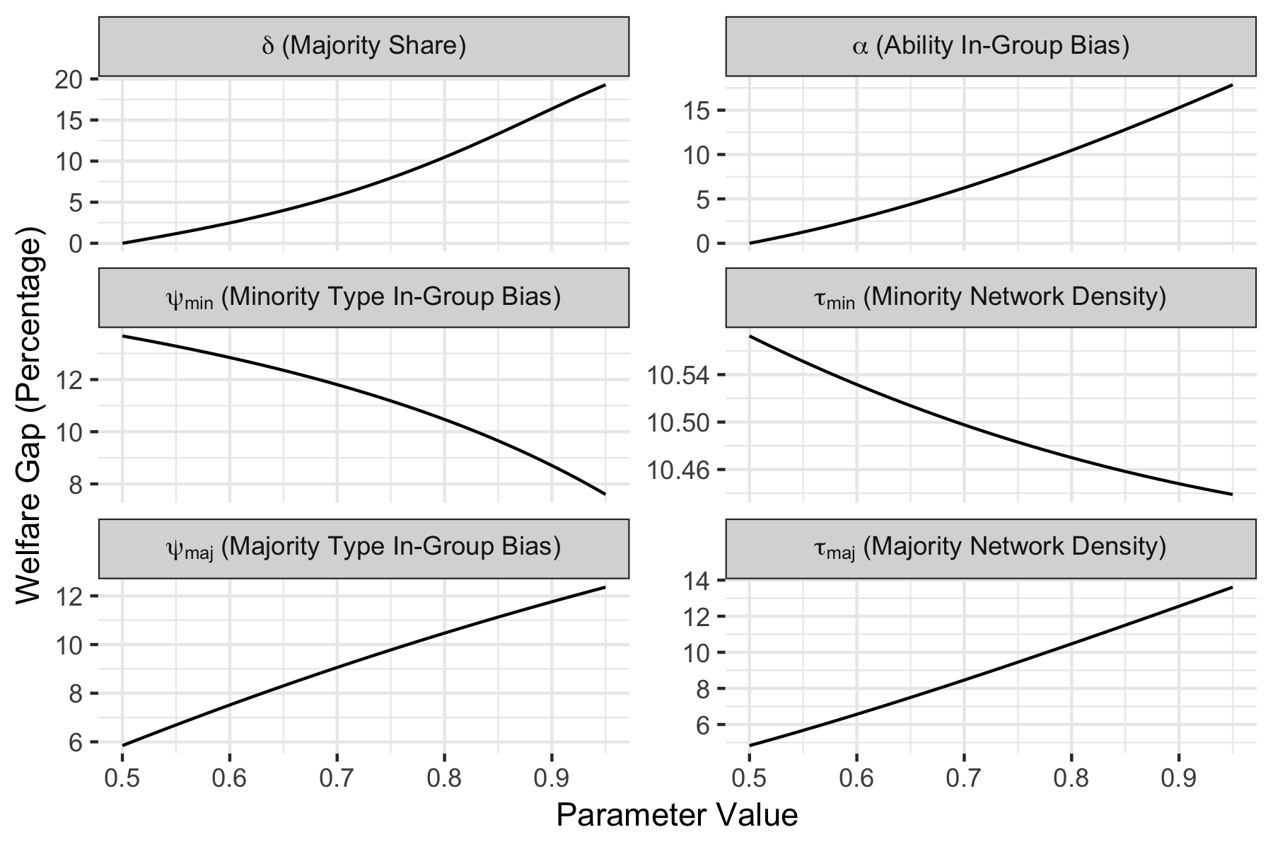
Figure III: Estimated Welfare Gap of Minority Workers^*

^*In each chart, the parameters not being varied all equal 0.8.

Welfare (i.e., expected wage) is calculated by summing the market wage ($w_{M2}$) and expected referral wage ($E(w_{R_{Hmaj}})$ or $E(w_{R_{Hmin}})$), weighted by the likelihood of the worker’s type gaining employment through the market or through referrals, respectively. Figure III plots the estimated welfare gap between majority and minority workers as a function of various network parameters. The welfare gap increases in $\delta$, $\alpha$, $\psi_{maj}$, and $\tau_{maj}$. It decreases in $\psi_{min}$ and $\tau_{min}$. Of note, the welfare gap increases convexly as the majority group occupies a greater share of the labor force.

4 Discussion

If the majority/minority type in the model is based on race, then the setting would correspond with a “race-blind” or “colorblind” setting. This is because workers are observationally equivalent, and so firms cannot incorporate race into hiring decisions. Due to the historical context of race in the United States, past research has found bias in favor of the majority group (see, e.g., [6]). The presence of such bias would exacerbate the disparities already predicted by the model in this paper.

This paper employs a parameterization of homophily that implies the relationship between $\Pr\{$Period-1 worker knows own majority/minority type$\}$ and in-group bias is not linear. To understand why, consider an individual worker from each social group. For the majority worker, any given magnitude of bias in favor of same-group social ties operates on a greater share of the population than it does for a minority worker. Hence, one would expect the parameterization of homophily to have some multiplicative relationship with the share of the labor force, which a simple linear parameterization would not have. Furthermore, one would expect any given magnitude of homophily to have an amplified effect on the likelihood of having a same-group social tie for a given majority worker compared to a given minority worker.

The relationship between this paper’s parameterization of in-group bias and the incidence of social ties can be seen in Figure IV. Specifically, Figure IV illustrates the sensitivity of same-group social ties ($\phi$) to the in-group bias parameter ($\psi$). This relationship is based on the expression linking share of the labor force ($w$) to in-group bias described in Equation 1 of Proposition 1:

$$\Pr\{\text{period-1 worker knows own maj/min type}\}=\phi=\frac{w\cdot\psi}{[w\cdot\psi]+[(1-w)(1-\psi)]}$$

(The simplified numerical example immediately following Proposition 1 in the Equilibrium Section illustrates the logic of this expression.) When $\psi=0.5$, there is no bias (i.e., probability of social ties with the same type = $w$); when $\psi=1$, there is full bias (i.e., probability of social ties with the same type = 1). The dashed line represents a linear scaling, in which there is no amplification/dampening effect for majority and minority workers. Though not included in the graph below, the specification used in this article yields a linear relationship if both workers’ groups occupy 50% of the labor force (i.e., when social groups are the same size there is no amplification/dampening effect).

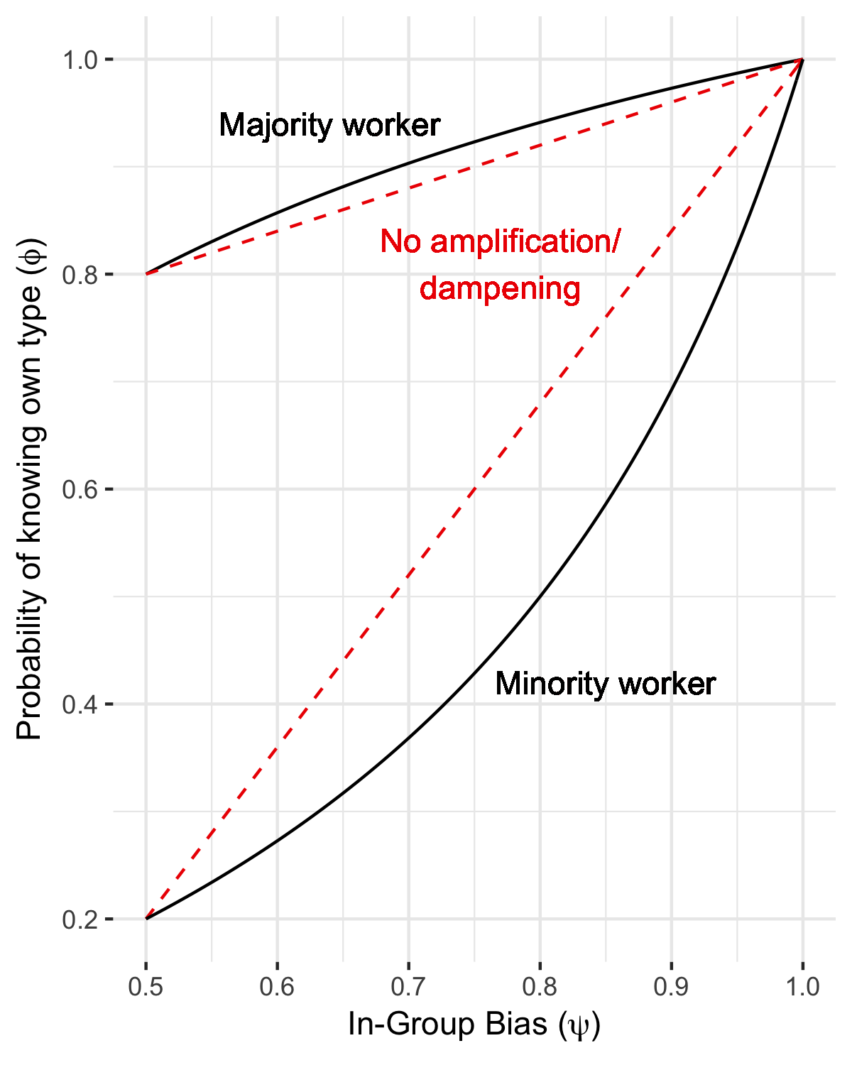
Figure IV: Social Tie Sensitivity to In-Group Bias^*

^*where majority share of the labor force is 80%

The findings in this paper related to the unequal distribution of referral offers are robust to specifications for bias—e.g., Equation 1 from Proposition 1—where the relationship between the probability of knowing one’s own type ($\phi$) and the bias ($\psi$) is more concave for majority workers than for minority workers. In other words, it is robust to specifications where there is a comparative amplification effect on the incidence of same-group social ties for majority workers (as seen in Figure IV). This relationship captures the fact that an equal magnitude of bias has a disproportionately larger impact on majority workers than on minority workers.

Recall that the predicted inequality between majority and minority workers is based on several assumptions, which include: (1) majority and minority workers have no labor market disparities in the initial time period; (2) the only distinguishable difference between groups is relative size (i.e., ability, network density, and in-group biases are all equivalent); (3) workers are more likely to know others with similar characteristics; and (4) there is no psychological prejudice. These assumptions are critical when considering historical examples where minority workers enjoy greater welfare than majority workers (e.g., white South Africans), or when particular demographic groups who comprise a majority of a local labor market face worse outcomes (e.g., black workers in a variety of U.S. metropolitan areas). These cases do not undermine the accuracy of the model, not only because their circumstances clearly violate the model’s assumptions (e.g., that there is full equality between groups in the initial time period), but also because these cases intimately involve the distorting influence or legacy of psychological prejudice, which the employment model explicitly and intentionally does not incorporate.

5 Calibration

This section calibrates the model to assess, in one application, the magnitudes of model parameters—such as majority and minority type in-group bias and network density—and to estimate a lower bound for the magnitude of inequality arising from social network discrimination. The setting for this calibration exercise is the Public Use data from the National Longitudinal Study of Adolescent to Adult Health, 1994–2008 [20]. This data consists of a nationally representative sample of U.S. adolescents in grades 7 through 12 during the 1994–1995 school year. In the friendship section of the in-school questionnaire, which was administered to over 90,000 students attending 145 schools in 80 communities, the respondents were asked to nominate up to five male and five female friends from the roster of all students enrolled. This information was used to construct social network parameters, which are adapted below to estimate the parameters in this paper’s model. Further details about the overall sample and design of the study are provided in [38]. I make some simplifying assumptions for the purpose of this calibration, such as assuming that the social network parameters of the respondents do not change from childhood through their eventual entry into the labor market.

5.1 Calibrated Social Network Parameters

For the purpose of this calibration exercise, white respondents represent the majority and black respondents represent the minority. Here I define some of the terms used below in the calibration data: ego means respondent; alter means the student in the same school as ego who is eligible to be nominated as a friend; node means a unique member of a network; and ego’s send-network means the ego and the set of alters nominated by the ego as friends. Social network parameters are calculated as follows:

Majority share ($\delta$)—This parameter is calculated by taking the total count of white respondents in the calibration data and dividing it by the total count of white respondents plus black respondents. Based on this definition, $\delta=0.70$.

Ability in-group bias ($\alpha$)—For simplicity, I assume $\alpha=1$.

Network density ($\tau_{maj}$ and $\tau_{min}$)—These parameters are calculated based on the calibration data parameter “ego send-network density” for white and black respondents. The ego send-network density is defined as the density of the network composed of ego and the set of alters nominated by ego:

$$ESDEN_{i}=\frac{\sum S}{s\cdot(s-1)}\hskip 2.84544pt\text{,}$$

where:

$$S=\text{total ego send-network}$$

$$s=\text{number of nodes in S}$$

Based on this definition, let:

$$\tau_{maj}=mean(ESDEN_{i\text{ for }i\in{\text{white respondents}}})\hskip 2.84544pt\text{, and}$$

$$\tau_{min}=mean(ESDEN_{i\text{ for }i\in{\text{black respondents}}})$$

Substituting values from the calibration data, $\tau_{maj}=0.41$ and $\tau_{min}=0.43$.

Type in-group bias ($\psi_{maj}$ and $\psi_{min}$)—These parameters are calculated based on the calibration data parameter “ego-network heterogeneity measure for race.” The ego-network heterogeneity assesses the heterogeneity of the respondent’s network with respect to race. The formula used to calculate the ego-network heterogeneity for respondent $i$ is:

$$HETEROGENEITY_{iR}=1-\left[\sum^{n}_{k=1}\left(\frac{R_{k}}{d}\right)^{2}\right]\hskip 2.84544pt\text{,}$$

where:

$$R=\text{the race attribute}$$

$$R_{k}=\text{the number of nodes with race }k\text{ in the ego network}$$

$$d=\text{the number of nodes in the ego network with valid data on }R$$

$$n=\text{the total number of races of }R\text{ represented in the ego network}$$

If all members of the respondent’s network who have valid data on race share the same race, $HETEROGENEITY_{iR}=0$. Based on the range of the parameter $HETEROGENEITY_{iR}$, I perform a simple transformation and take the mean to estimate the parameters $\psi_{maj}$ and $\psi_{min}$ (which, by definition, range between $\frac{1}{2}$ and $1$):

$$\psi_{maj}=mean\left(1-\frac{HETEROGENEITY_{iR\text{ for i}\in\text{white respondents}}}{2}\right)\hskip 2.84544pt\text{, and}$$

$$\psi_{min}=mean\left(1-\frac{HETEROGENEITY_{iR\text{ for i}\in\text{black respondents}}}{2}\right)$$

Substituting values from the calibration data, $\psi_{maj}=0.87$ and $\psi_{min}=0.83$.

5.2 Inequality Arising From Social Network Discrimination

Let us now take the calibrated model parameters, calculated above from a nationally-representative sample of social networks among white and black respondents, to estimate the degree of economic inequality deriving purely from social network discrimination. It is worth noting that the inequality predicted in this subsection is based on the counterfactual world introduced by the model: namely, that there is equal average ability, education, and initial employment between white and black workers. I assume that half of white respondents and half of black respondents are high-ability, and half of both racial groups are low-ability. Hence, the assumption moving forward is that the only difference between racial groups is in their social network parameters, not in the distribution of any attribute correlated with productivity or ability.

I have already calculated all relevant unknown parameters of our model in the previous subsection: $\delta=0.70$, $\alpha=1$, $\tau_{maj}=0.41$, $\tau_{min}=0.43$, $\psi_{maj}=0.87$, and $\psi_{min}=0.83$. I will begin by calculating the probability that white and black respondents refer others of the same race, using Equation 1 from Proposition 1. Adapting that equation to this calibration setting gives us the following two Expressions:

(1) $$\Pr\{\text{white respondent refers white person}\}=\phi_{maj}=\frac{\delta\cdot\psi_{maj}}{[\delta\cdot\psi_{maj}]+[(1-\delta)(1-\psi_{maj})]}$$

(2) $$\Pr\{\text{black respondent refers black person}\}=\phi_{min}=\frac{(1-\delta)\cdot\psi_{min}}{[(1-\delta)\cdot\psi_{min}]+[\delta\cdot(1-\psi_{min})]}$$

I substitute the calibrated parameter values to calculate $\phi_{maj}=0.94$ and $\phi_{min}=0.68$. It is worth noting that both black and white respondents disproportionately refer members of their own race (since $\delta=0.7$ and $1-\delta=0.3$), reflecting the influence of type in-group bias across both racial groups.

Next, I seek to determine the welfare gap—the difference in expected wage—between high-ability white and black respondents. Let $H_{maj}$ denote high-ability majority worker, $H_{min}$ denote high-ability minority worker, $L_{maj}$ denote low-ability majority worker, and $L_{min}$ denote low-ability minority worker. The steps I take to calculate the expected wage gap between high-ability black and white workers is as follows: (1) estimate the likelihood that a high-ability white worker accepts a referral wage, relative to the likelihood a high-ability black worker accepts a referral wage; (2) estimate the market wage and the expected referral wage for both racial groups; and (3) estimate the expected welfare gap between black and white workers by summing the market wage $w_{M2}$ and expected referral wage $E(w_{R_{k}})$, weighted by the likelihood of the worker’s racial group gaining employment through the general market or through the referral market, respectively.

5.2.1 Step 1: Estimate the relative likelihood between racial groups that a high-ability worker accepts a referral wage

As the Appendix explains, let $e^{X}$ denote the $Pr(X\text{ accepts the market wage})$, which can be calculated as follows:

$$\begin{split}e^{H_{maj}}&=\exp\{-[\delta\alpha\tau_{maj}\phi_{maj}+(1-\delta)\alpha\tau_{min}(1-\phi_{min})]\}\\ e^{H_{min}}&=\exp\{-[\delta\alpha\tau_{maj}(1-\phi_{maj})+(1-\delta)\alpha\tau_{min}\phi_{min}]\}\\ e^{L_{maj}}&=\exp\{-[\delta(1-\alpha)\tau_{maj}\phi_{maj}+(1-\delta)(1-\alpha)\tau_{min}(1-\phi_{min})]\}\\ e^{L_{min}}&=\exp\{-[\delta(1-\alpha)\tau_{maj}(1-\phi_{maj})+(1-\delta)(1-\alpha)\tau_{min}\phi_{min}]\}\end{split}$$

Then, the likelihood that a high-ability white worker accepts a referral wage, relative to the likelihood that a high-ability black worker accepts a referral wage can be calculated as follows:

$$\Pr\{H_{maj}\text{ accepts referral relative to }\Pr\{H_{min}\text{ accepts referral}\}\}=\gamma_{maj}=\frac{1-e^{H_{maj}}}{1-e^{H_{min}}}$$

Substituting calibration values results in $\gamma_{maj}=2.70$. By construction, $\gamma_{min}=1$.

5.2.2 Step 2: Estimate the market wage and the expected referral wage for both racial groups

Market wage—As the proof for Proposition 3 in the Appendix illustrates, Bayes’s rule allows one to calculate the period-2 market wage:

$$\begin{split}&w_{M2}(\alpha,\delta,\tau_{maj},\tau_{min},\psi_{maj},\psi_{min})\\ &=E(\text{productivity \textbar{} market})\\ &=\frac{\Pr(\text{market \textbar{} $H_{maj}$})\cdot\Pr(H_{maj})+\Pr(\text{market \textbar{} $H_{min}$})\cdot\Pr(H_{min})}{\Pr(\text{market \textbar{} $H$})\cdot\Pr(H)+\Pr(\text{market \textbar{} $L$})\cdot\Pr(L)}\\ &=\frac{(e^{H_{maj}}\cdot\delta)+(e^{H_{min}}\cdot(1-\delta))}{(e^{H_{maj}}+e^{L_{maj}})\cdot\delta+(e^{H_{min}}+e^{L_{min}})\cdot(1-\delta)}\end{split}$$

Substituting the calibrated model parameters results in $w_{M2}=0.44$. As the exposition for Proposition 2 mentions, $w_{M2}$ should always be below the average productivity of the workforce, which is 0.5. This is because homophily along ability (i.e., ability in-group bias) causes a disproportionately high volume of high-ability workers to be hired via referrals, which lowers the average productivity in the (non-referral) general market and drives down the equilibrium market wage.

Referral Wage—Adapting Appendix Equation A.7, any given referral wage ${w_{R_{k}}}$ can be expressed as:

(3) $$\begin{split}w_{R_{k}}=&\frac{\begin{aligned} &p^{H_{maj}}\cdot\exp\{-[p^{H_{maj}}][1-F(w_{R_{k}})\}+p^{H_{min}}\cdot\exp\{-[p^{H_{min}}][1-F({w_{R_{k}}})]\}-c\end{aligned}}{\begin{aligned} &p^{H_{maj}}\cdot\exp\{-[p^{H_{maj}}][1-F(w_{R_{k}})\}+p^{H_{min}}\cdot\exp\{-[p^{H_{min}}][1-F({w_{R_{k}}})]\}\\ &+p^{L_{maj}}\cdot\exp\{-[p^{L_{maj}}][1-F({w_{R_{k}}})]\}+p^{L_{min}}\cdot\exp\{-[p^{L_{min}}][1-F({w_{R_{k}}})]\}\end{aligned}}\end{split}$$

where $F(\bullet)$ represents the equilibrium wage distribution; $c$ represents the expected firm profit, which is constant across the entire wage distribution and can thus be set equal to the expected productivity in the (non-referral) general market; and $p^{X}$ is denoted as follows:

$$\begin{split}p^{H_{maj}}&=\delta\alpha\tau_{maj}\phi_{maj}+(1-\delta)\alpha\tau_{min}(1-\phi_{min})\\ p^{H_{min}}&=\delta\alpha\tau_{maj}(1-\phi_{maj})+(1-\delta)\alpha\tau_{min}\phi_{min}\\ p^{L_{maj}}&=\delta(1-\alpha)\tau_{maj}\phi_{maj}+(1-\delta)(1-\alpha)\tau_{min}(1-\phi_{min})\\ p^{L_{min}}&=\delta(1-\alpha)\tau_{maj}(1-\phi_{maj})+(1-\delta)(1-\alpha)\tau_{min}\phi_{min}\\ \\ c=E\prod_{H}(w_{M2})&=(p^{HMAJ})(e^{HMAJ})(1-w_{M2})+(p^{HMIN})(e^{HMIN})(1-w_{M2})\\ &\qquad+(p^{LMAJ})(e^{LMAJ})(-w_{M2})+(p^{LMIN})(e^{LMIN})(-w_{M2})\end{split}$$

For simplicity, I assume a uniform equilibrium wage distribution $F(\bullet)$ and so have normalized the value for the average referral wage for black workers—$F(w_{R_{k}}^{H_{min}})$—to $0.5$ (since in Step 1 we normalized $\gamma_{min}=1$). I then estimate $F(w_{R_{k}}^{H_{maj}})$ for the referral wage for white workers. Since workers accept the maximum referral wage offered, estimating $F(w_{R_{k}}^{H_{maj}})$ is akin to finding the expected value of the maximum of $\gamma_{maj}$ random variables:

$$F(w_{R_{k}}^{H_{maj}})=\frac{\gamma_{maj}}{\gamma_{maj}+1}$$

Substituting the value for $\gamma_{maj}$ calculated in Step 1, one can estimate that $F(w_{R_{k}}^{H_{maj}})=0.73$. Substituting the calibration parameter values, the value for $F(w_{R_{k}}^{H_{maj}})$, and the value for $F(w_{R_{k}}^{H_{min}})$ into Expression 3 results in $E(w_{R_{k}}^{H_{maj}})=0.534$ and $E(w_{R_{k}}^{H_{min}})=0.5063$.

5.2.3 Step 3: Estimate the expected welfare gap between racial groups

To calculate the expected welfare gap between black and white workers, I take the sum of the market wage and the expected referral wage, weighted by the likelihood of being hired via the general market or via the referral market, respectively:

Welfare gap $$=1-\frac{\Pr(H_{min}\text{ accepts }w_{M2})\cdot w_{M2}+\Pr(H_{min}\text{ accepts }w_{R})\cdot E(w_{R_{k}}^{H_{min}})}{\Pr(H_{maj}\text{ accepts }w_{M2})\cdot w_{M2}+\Pr(H_{maj}\text{ accepts }w_{R})\cdot E(w_{R_{k}}^{H_{maj}})}$$

$$=1-\frac{e^{H_{min}}\cdot w_{M2}+(1-e^{H_{min}})\cdot E(w_{R_{k}}^{H_{min}})}{e^{H_{maj}}\cdot w_{M2}+(1-e^{H_{maj}})\cdot E(w_{R_{k}}^{H_{maj}})}$$

Substituting calibration parameter values gives a welfare gap—which is the difference in expected wages in this model—of 4.04 percent between racial groups, with black workers being disadvantaged compared to white workers. This welfare gap is driven by two factors: (1) the disproportionately high likelihood that black workers will be hired through the (non-referral) general market, which pays the lowest wage on the equilibrium wage distribution; and (2) the disproportionately high volume of referrals white workers receive, which increases the maximum referral wage white workers are able to eventually accept compared to black workers.

It is important to remember that this estimated welfare gap between black and white workers is based on a key simplifying assumption of the model: namely, that both the majority and minority groups begin the first period in a state of equality. In other words, the welfare gap of 4.04 percent is what the model estimates over time given an initial state of equality between racial groups. Yet in the U.S. context, initial equality between racial groups did not exist; black workers not only may be negatively impacted today by persisting social network discrimination (as suggested above), but also they have been harmed historically by the remnants of past discrimination (which is outside the scope of this paper’s analysis). Historical discrimination would plausibly exacerbate the inequalities in referral opportunities between black and white workers—even conditional on the same magnitude of the underlying social network parameters. As such, the estimated welfare gap from the calibration exercise may represent a lower bound of the true extent to which social network discrimination contributes to racial inequality in the U.S. context.

6 Conclusion

Social network discrimination reveals that referral systems and related hiring practices may inadvertently contribute to structural racism in the absence of race-conscious policies. Furthermore, the mechanism of discrimination uncovered by this paper is relevant to a wide variety of other real-world contexts. For example, important social ties are formed in postsecondary schooling (e.g., colleges and universities), in professional schools (e.g., business schools, law schools, and medical schools), and in workplaces. There might be inherent social network advantages associated with belonging to a larger demographic group, all else equal, since the formation of such ties are influenced by social phenomena like homophily. In turn, social ties formed in these settings may not only prove instrumental for future referral opportunities, they may also extend to contexts beyond the labor market—for example, to any setting in which opportunities are allocated based on informal information networks. In short, social network discrimination may distort the allocation of personal, educational, and professional opportunities in ways previously unexplored—an important insight that not only may help explain substantial inequalities that persist between demographic groups today, but also may help inform efforts to promote equitable access to opportunity in the future.

Appendix

Lemma 2

A firm will attempt to hire through referral if and only if it employs a high-ability worker in period 1.

Proof. Firms employing high-ability workers in period 1 will make referral offers for two reasons. First, hiring through the market yields zero expected profit (given the assumption of free entry of firms). Second, an accepted referral offer yields constant positive profit over the range of the referral offer wage distribution $[w_{M2},\overline{w}_{R}]$. (If it did not yield constant positive profits, it would be impossible to maintain equilibrium wage dispersion; the profit-maximizing firms would offer only a subset of the distribution—i.e., those wages that maximized profits.) An offer below $w_{M2}$ will never be accepted, while an offer above $\overline{w}_{R}$ increases the wage without increasing the probability of attracting a worker. To complete the proof of this lemma, I show that firms employing low-ability workers in period 1 will hire through the market (i.e., not rely on referrals).

If a firm employing a low-ability worker did deviate from this Lemma and made a referral offer $w_{R}$, its expected profit (denoted $E\prod_{L}(w_{R})$) would be represented by a slight modification to the expression for the expected profit for a firm employing a high-ability worker (denoted $E\prod_{H}(w_{R})$ and derived in Equation A.6 of Proposition 3). The expression for $E\prod_{L}(w_{R})$ differs from that of $E\prod_{H}(w_{R})$ in that the incidences of $\alpha$ in the first $p^{HMAJ}$, $p^{HMIN}$, $p^{LMAJ}$, and $p^{LMIN}$ terms are replaced with ($1-\alpha$), and vice versa.

In this scenario, as long as $\alpha>\frac{1}{2}$, $E\prod_{L}(w_{R})<0$. Hence, expected profits are less than those from hiring in the general market, which equals zero due to free entry of firms. The lemma is thus proved: a firm employing a low-ability worker in period-1 prefers to hire through the market, maximizing expected profit.   

Lemma 3

The period-1 market wage is greater than the expected period-1 productivity.

Proof. Firms hiring in the period-1 market earn an expected period-2 profit equal to the probability of obtaining a high-ability period-1 worker times the expected profit (denoted $c$) from a referral. Free entry thus drives the wage above expected period-1 productivity:

$$w_{M1}(\alpha,\delta,\tau_{maj},\tau_{min},\psi_{maj},\psi_{min})$$

$$=\frac{1}{2}+\frac{1}{2}c(\alpha,\delta,\tau_{maj},\tau_{min},\psi_{maj},\psi_{min})$$

$$=\frac{1}{2}[1+c(\alpha,\delta,\tau_{maj},\tau_{min},\psi_{maj},\psi_{min})]$$

The expression for $c$ is derived in Proposition 3. Given comparative-statics results on $c$, $w_{M1}$ is increasing in $\tau_{maj}$ and $\tau_{min}$. When both $\tau_{maj}=\tau_{min}$ and $\psi_{maj}=\psi_{min}$, $w_{M1}$ is decreasing in $\delta$.   

Proposition 1A

In an environment with equal magnitude of majority/minority network parameters ($\tau_{maj}=\tau_{min}$ and $\psi_{maj}=\psi_{min}$), the probability a high-ability minority worker in period 2 receives a referral offer is lower than their share of the labor force. The inverse holds for majority workers:

$$\Pr\{\text{period-2 high-ability minority worker receives referral offer}\}<\frac{1-\delta}{2}$$

$$\Pr\{\text{period-2 high-ability majority worker receives referral offer}\}>\frac{\delta}{2}$$

Proposition 1B

The inequality in the distribution of referral job offers can be eliminated by minority workers having a sufficiently higher type in-group bias ($\psi_{min}$).

Proof. Let us first consider a given high-ability period-2 worker ($H$). Since all referral wage offers are above the period-2 market wage, the probability that $H$ would accept a referral wage offer $w_{Ri}$ from firm $i$ can be expressed:

$$\Pr\{\text{$H$ accepts $w_{Ri}$}\}=\Pr\{\text{$H$ receives no higher offer $w_{Rj}\ \forall$ firm $j\neq i$}\}$$

Since referral offers are allocated independently,

$$\Pr\{\text{$H$ accepts $w_{Ri}$}\} =\prod_{j\neq i}\Pr\{\text{$H$ receives no higher offer $w_{Rj}$}\}$$

$$=\prod_{j\neq i}[\operatorname*{}1-\Pr\{\text{$H$ receives an offer $w_{Rj}>w_{Ri}$}\}]$$

The probability that firm $j$ offers a wage $w_{Rj}>w_{Ri}$ to $H$ is the product of two independent probabilities:

$$\Pr\{\text{$H$ receives an offer $w_{Rj}>w_{Ri}$}\}=\Pr\{\text{firm $j$ makes offer to $H$}\}\cdot\Pr\{w_{Rj}>w_{Ri}\}$$

If $2N$ workers were in period-1, free entry implies that $N$ firms employ high-ability workers. Now I will analyze both parts of the expression from the perspective of a high-ability majority worker ($H_{maj}$) and high-ability minority worker ($H_{min}$).

The probability that firm $j$ offers a referral to $H_{maj}$ is a weighted average of whether firm $j$ hired a majority or minority worker in period 1. Denote $\phi_{maj}$ as the probability a majority worker knows another majority worker, and $\phi_{min}$ as the probability a minority worker knows another minority worker, where:

$$\phi_{maj}=\frac{\left(\delta\cdot\psi_{maj}\right)}{\left(\delta\cdot\psi_{maj}\right)+[(1-\delta)\cdot(1-\psi_{maj})]}\hskip 2.84544pt\text{, and}$$

$$\phi_{min}=\frac{(1-\delta)\cdot\psi_{min}}{[(1-\delta)\cdot\psi_{min}]+[\delta\cdot(1-\ \psi_{min})]}\hskip 28.45274pt$$

Then:

(A.1) $$\begin{split}&\Pr\{\text{firm $j$ makes offer to $H_{maj}$}\}=\delta\left(\frac{\alpha\tau_{maj}\phi_{maj}}{N}\right)+(1-\delta)\genfrac{(}{)}{}{}{\alpha\tau_{min}(1-\phi_{min})}{N}\end{split}$$

Likewise, for a period-2 minority high-ability worker:

$$\Pr\{\text{firm $j$ makes offer to $H_{min}$}\}=\delta\left(\frac{\alpha\tau_{maj}(1-\phi_{maj})}{N}\right)+(1-\delta)\genfrac{(}{)}{}{}{\alpha\tau_{min}\phi_{min}}{N}$$

Based on these expressions, for minority workers to have a proportional chance of receiving job offers through referral, the following must hold:

$$\begin{gathered}\Pr\{\text{firms make offer to $H_{maj}$}\}\propto\Pr\{\text{firms make offer to $H_{min}$}\}\\ \\ \text{only when}\\ \\ (1-\delta)\left[\delta\tau_{maj}\phi_{maj}+(1-\delta)\tau_{min}(1-\phi_{min})\right]=\delta\left[\delta\tau_{maj}(1-\phi_{maj})+(1-\delta)\tau_{min}(\phi_{min})\right]\end{gathered}$$

Both the minority network density required to compensate for the inequality (denoted $\tau_{min}^{=}$) and the minority type in-group bias required to compensate (denoted $\psi_{min}^{=}$) increase in $\tau_{maj}$, $\psi_{maj}$, and $\delta$. The greater the probability of majority workers having social ties (or the greater the degree of their type in-group bias or likelihood of possessing social ties), the greater minority workers’ compensating parameters ($\tau_{min}^{=}$ or $\psi_{min}^{=}$) must be to achieve a proportional amount of all job offers through referrals.

Though higher minority network density and type in-group bias can both reduce the disproportionality in the distribution of job offers through referral, analysis shows that between these two parameters only $\psi_{min}^{=}$ is attainable (i.e., below 1) under all possible combinations of social network parameters.   

Proposition 2

In an environment with equal magnitude of majority/minority network parameters ($\tau_{maj}=\tau_{min}$ and $\psi_{maj}=\psi_{min}$), the period-2 market wage ($w_{M2}$) decreases as majority workers occupy a greater fraction of the labor force. $w_{M2}$ also decreases in the ability in-group bias $\alpha$.

Proof. First I derive an expression for period-2 market wage. I build on the analysis from Proposition 1. If there were $2N$ workers in period 1, free entry implies that $N$ firms employ high-ability workers. If firms select their referral wage offer by randomizing over the equilibrium wage distribution $F(\bullet)$ (to be derived below),

$$\Pr\{\text{$H_{maj}$ receives an offer $w_{Rj}>w_{Ri}$}\}=\Pr\{\text{firm $j$ makes offer to $H_{maj}$}\}\cdot[1-F(w_{Ri})]$$

for all firms $j$ who employ a high-ability worker in period 1. I have already shown that:

$$\Pr\{\text{$H$ accepts $w_{Ri}$}\} =\prod_{j\neq i}\Pr\{\text{$H$ receives no higher offer $w_{Rj}$}\}$$

$$=\prod_{j\neq i}[\operatorname*{}1-\Pr\{\text{$H$ receives an offer $w_{Rj}>w_{Ri}$}\}]$$

Substitution yields:

$$\Pr\{\text{$H_{maj}$ accepts $w_{Ri}$}\}$$

$$=\{1-[\frac{1}{N}(\delta\alpha\tau_{maj}\phi_{maj}+(1-\delta)\alpha\tau_{min}(1-\phi_{min}))]\cdot[1-F(w_{Ri})]\}^{N-1}$$

Since the model assumes a large number of workers, as $N$ approaches $\infty$,

(A.2) $$\Pr\{\text{$H_{maj}$ accepts $w_{Ri}$}\}=\exp\{-[\delta\alpha\tau_{maj}\phi_{maj}+(1-\delta)\alpha\tau_{min}(1-\phi_{min})][1-F(w_{Ri})]\}$$

Details on this step can be found in [35] and [31]. One can use similar steps to obtain the probability that firm $i$’s offer is accepted by a given high-ability majority worker ($H_{maj}$), low-ability majority worker($L_{maj}$), and low-ability minority worker($L_{min}$).

As high-ability workers tend to receive more offers, they are less likely to accept any given offer $w_{Ri}<\overline{w}_{R}$. Since a period-2 worker finds employment through the market only if he receives no offers (or rejects all referral offers):

$$\Pr\{\text{market \textbar{} $H_{maj}$}\}=\Pr\{\text{$H_{maj}$ accept $w_{M2}$}\}$$

The market wage coincides with the bottom of the referral wage distribution, $F(\bullet)$, because any referral wage below the market wage will be rejected by period-2 workers, to gain employment through the market. Thus, given that $F(w_{M2})=0$:

$$\Pr\{\text{market \textbar{} $H_{maj}$}\}=\exp\{-[\delta\alpha\tau_{maj}\phi_{maj}+(1-\delta)\alpha\tau_{min}(1-\phi_{min})]\}$$

I can derive similar expressions for $H_{min}$, $L_{maj}$, and $L_{min}$. Let:

(A.3) $$\begin{split}e^{HMAJ}&=\exp\{-[\delta\alpha\tau_{maj}\phi_{maj}+(1-\delta)\alpha\tau_{min}(1-\phi_{min})]\}\\ e^{HMIN}&=\exp\{-[\delta\alpha\tau_{maj}(1-\phi_{maj})+(1-\delta)\alpha\tau_{min}\phi_{min}]\}\\ e^{LMAJ}&=\exp\{-[\delta(1-\alpha)\tau_{maj}\phi_{maj}+(1-\delta)(1-\alpha)\tau_{min}(1-\phi_{min})]\}\\ e^{LMIN}&=\exp\{-[\delta(1-\alpha)\tau_{maj}(1-\phi_{maj})+(1-\delta)(1-\alpha)\tau_{min}\phi_{min}]\}\end{split}$$

I now use Bayes’s rule to calculate the period-2 market wage:

(A.4) $$\begin{split}&w_{M2}(\alpha,\delta,\tau_{maj},\tau_{min},\psi_{maj},\psi_{min})\\ &=E(\text{productivity \textbar{} market})\\ &=\frac{\Pr(\text{market \textbar{} $H_{maj}$})\cdot\Pr(H_{maj})+\Pr(\text{market \textbar{} $H_{min}$})\cdot\Pr(H_{min})}{\Pr(\text{market \textbar{} $H$})\cdot\Pr(H)+\Pr(\text{market \textbar{} $L$})\cdot\Pr(L)}\\ &=\frac{(e^{HMAJ}\cdot\delta)+(e^{HMIN}\cdot(1-\delta))}{(e^{HMAJ}+e^{LMAJ})\cdot\delta+(e^{HMIN}+e^{LMIN})\cdot(1-\delta)}\end{split}$$

Given $\alpha>\frac{1}{2}$ and both network densities ($\tau_{maj}$ and $\tau_{min}$) greater than zero, $w_{M2}$ is always less than $\frac{1}{2}$, the average productivity of the population. Analysis shows that $w_{M2}$ is decreasing in $\alpha$. Furthermore, for all $\psi_{maj}=\psi_{min}$ and $\tau_{maj}=\tau_{min}$, $w_{M2}$ is also decreasing in $\delta$.   

Proposition 3

In an environment with equal magnitude of majority/minority network parameters ($\tau_{maj}=\tau_{min}$ and $\psi_{maj}=\psi_{min}$), the referral wage and the welfare (i.e., average expected wage) for minority workers is lower than for majority workers.

Proof. Consider the expected period-2 profit earned by a firm employing a high-ability worker and setting a referral wage (recall the productivity of high-ability workers equals one, while that of low-ability workers equals zero):

$E\prod_{H}(w_{R})$

$$=\Pr\{\text{high-ability majority period-2 referral hired \textbar{} $w_{R}$}\}\cdot(1-w_{R})$$

$$\qquad+\Pr\{\text{high-ability minority period-2 referral hired \textbar{} $w_{R}$}\}\cdot(1-w_{R})$$

$$\qquad+\Pr\{\text{low-ability majority period-2 referral hired \textbar{} $w_{R}$}\}\cdot(-w_{R})$$

$$\qquad+\Pr\{\text{low-ability minority period-2 referral hired \textbar{} $w_{R}$}\}\cdot(-w_{R})$$

(If no referred worker is hired, perhaps because the period-1 worker possesses no social tie or because the referred acquaintance receives a better offer, the firm hires through the market and earns zero expected profit.)

The probability of hiring a high-ability majority period-2 referred worker is the product of two independent probabilities (substituting from Equations A.1 and A.2 from Propositions 1 and 2):

$$\Pr\{\text{high-ability period-2 majority referral hired \textbar{} $w_{R}$}\}$$

$$=\Pr\{\text{offer made to a high-ability majority referral}\}\cdot\Pr\{\text{$H_{maj}$ accepts $w_{R}$}\}$$

$$=\delta\alpha\tau_{maj}\phi_{maj}\ +(1-\delta)\alpha\tau_{min}(1-\phi_{min})$$

$$\qquad\cdot\exp\{-[\delta\alpha\tau_{maj}\phi_{maj}+(1-\delta)\alpha\tau_{min}(1-\phi_{min})][1-F(w_{R})]\}$$

Similar steps can be followed to derive the respective conditional probability for high-ability minority, low-ability majority, and low-ability minority workers.

Let:

(A.5) $$\begin{split}p^{HMAJ}&=\delta\alpha\tau_{maj}\phi_{maj}+(1-\delta)\alpha\tau_{min}(1-\phi_{min})\\ p^{HMIN}&=\delta\alpha\tau_{maj}(1-\phi_{maj})+(1-\delta)\alpha\tau_{min}\phi_{min}\\ p^{LMAJ}&=\delta(1-\alpha)\tau_{maj}\phi_{maj}+(1-\delta)(1-\alpha)\tau_{min}(1-\phi_{min})\\ p^{LMIN}&=\delta(1-\alpha)\tau_{maj}(1-\phi_{maj})+(1-\delta)(1-\alpha)\tau_{min}\phi_{min}\end{split}$$

So, to simplify:

$E\prod_{H}(w_{R})$

(A.6) $$\begin{split}&=p^{HMAJ}\cdot\exp\{-[p^{HMAJ}][1-F(w_{Ri})]\}\cdot(1-w_{R})\\ &\qquad+p^{HMIN}\cdot\exp\{-[p^{HMIN}][1-F(w_{Ri})]\}\cdot(1-w_{R})\\ &\qquad+p^{LMAJ}\cdot\exp\{-[p^{LMAJ}][1-F(w_{Ri})]\}\cdot(-w_{R})\\ &\qquad+p^{LMIN}\cdot\exp\{-[p^{LMIN}][1-F(w_{Ri})]\}\cdot(-w_{R})\end{split}$$

To maintain equilibrium wage dispersion, firms must earn the same expected profit on each referral wage offered:

$$E\prod_{H}(w_{R})=c\qquad\forall w_{R}\in[w_{M2},\overline{w}_{R}]$$

To calculate this profit constant, note that the firm could deviate from the specified strategy and offer a wage of $w_{M2}$; in this case, the referred worker accepts the firm’s offer only if they receive no other offers.

Recall that $F(w_{M2})=0$. The firm’s expected profit is therefore given by (using terms defined in Equations A.3 and A.5):

$$E\prod_{H}(w_{M2})$$

$$=(p^{HMAJ})(e^{HMAJ})(1-w_{M2})+(p^{HMIN})(e^{HMIN})(1-w_{M2})$$

$$\qquad+(p^{LMAJ})(e^{LMAJ})(-w_{M2})+(p^{LMIN})(e^{LMIN})(-w_{M2})$$

$$=c$$

Substituting for $w_{M2}$ (Equation A.4), I can determine $c(\alpha,\delta,\tau_{maj},\tau_{min},\psi_{maj},\psi_{min})$. Given $\alpha>\frac{1}{2}$, firms with high-ability workers who possess social ties earn positive expected profits. Analysis shows that $c$ is increasing in $\alpha$, $\tau_{maj}$, and $\tau_{min}$. When both $\psi_{maj}=\psi_{min}$ and $\tau_{maj}=\tau_{min}$, $c$ is decreasing in $\delta$.

Given the expression for $c(\alpha,\delta,\tau_{maj},\tau_{min},\psi_{maj},\psi_{min})$, the equilibrium referral-offer distribution $F(\bullet)$ can be determined by setting $E\prod_{H}(w_{R})$ (Equation A.6) equal to $c$ for all potential wage offers $w_{R}$.

Unfortunately, doing so does not yield a closed-form solution for $F(w_{R})$. Given a continuum of firms, the equilibrium referral-offer distribution $F(\bullet)$ can be interpreted as either: (1) each firm randomizes over the entire distribution; or (2) a fraction $f(w_{R})$ of firms offers each wage for sure.

From the second interpretation, one can denote these referral wages with $w_{Rk}$ and estimate the average referral wage received by a high-ability majority worker (denoted $E(w_{R_{Hmaj}})$) vs. a high-ability minority worker (denoted $E(w_{R_{Hmin}})$), for any given $\delta$, $\alpha$, $\tau_{maj}$, $\tau_{min}$, $\psi_{maj}$, and $\psi_{min}$. Analysis shows that in an environment with equal magnitude of majority/minority network parameters, if $\alpha>\frac{1}{2}$ and $\delta>\frac{1}{2}$, $E(w_{R_{Hmaj}})>E(w_{R_{Hmin}})$.

Proposition 1 shows that, all else equal, minority workers receive a smaller proportion of jobs through referral than their fraction of the population. As a result, minority workers more frequently gain employment through the market, receiving the (lower) market wage. In this Proposition, I showed that even when offered a job through referral, minority workers have lower expected referral wages than majority workers.  

To conclude, one can derive an expression for the maximum referral wage offered $\overline{w}_{R}$ (where $F(\overline{w}_{R})=1$, by definition):

(A.7) $$\overline{w}_{R}(\alpha,\delta,\tau_{maj},\tau_{min},\psi_{maj},\psi_{min})=\frac{p^{HMAJ}+p^{HMIN}-c}{p^{HMAJ}+p^{HMIN}+p^{LMAJ}+p^{LMIN}}$$

A firm that offers a referral wage of $\overline{w}_{R}$ attracts a referred worker with probability 1 (conditional on its period-1 worker possessing a social tie). The firm’s expected profit, $c$, is thus equal to $p^{HMAJ}+p^{HMIN}-\overline{w}_{R}(p^{HMAJ}+p^{HMIN}+p^{LMAJ}+p^{LMIN})$. $\overline{w}_{R}$ is increasing in $\alpha$, $\tau_{maj}$, and $\tau_{min}$.

References

- [1] Alberto Alesina, Stefanie Stantcheva and Edoardo Teso “Intergenerational Mobility and Preferences for Redistribution” In American Economic Review 108.2, 2018, pp. 521–54
- [2] Kenneth J Arrow and Ron Borzekowski “Limited Network Connections and the Distribution of Wages”, 2004
- [3] Vivek Ashok, Ilyana Kuziemko and Ebonya Washington “Demand for Redistribution in an Age of Rising Inequality: Some Mew Stylized Facts and Tentative Explanations” In Brookings Papers on Economic Activity, Spring, 2015, pp. 367–405
- [4] Patrick Bayer and Kerwin Kofi Charles “Divergent Paths: A New Perspective on Earnings Differences Between Black and White Men Since 1940” In The Quarterly Journal of Economics 133.3 Oxford University Press, 2018, pp. 1459–1501
- [5] Patrick Bayer, Stephen L Ross and Giorgio Topa “Place of Work and Place of Residence: Informal Hiring Networks and Labor Market Outcomes” In Journal of Political Economy 116.6 The University of Chicago Press, 2008, pp. 1150–1196
- [6] Marianne Bertrand and Sendhil Mullainathan “Are Emily and Greg More Employable than Lakisha and Jamal? A Field Experiment on Labor Market Discrimination” In American Economic Review 94.4, 2004, pp. 991–1013
- [7] Peter Michael Blau “Inequality and Heterogeneity: A Primitive Theory of Social Structure” Free Press New York, 1977
- [8] Lukas Bolte, Nicole Immorlica and Matthew O Jackson “The Role of Referrals in Inequality, Immobility, and Inefficiency in Labor Markets” In Working Paper, 2020
- [9] Ioan Sebastian Buhai and Marco J Leij “A social network analysis of occupational segregation” In arXiv preprint arXiv:2004.09293, 2020
- [10] Kenneth Burdett and Kenneth L Judd “Equilibrium Price Dispersion” In Econometrica: Journal of the Econometric Society JSTOR, 1983, pp. 955–969
- [11] Stephen V Burks, Bo Cowgill, Mitchell Hoffman and Michael Housman “The Value of Hiring Through Employee Referrals” In The Quarterly Journal of Economics 130.2 MIT Press, 2015, pp. 805–839
- [12] GR Butters “Equilibrium Distribution of Prices and Advertising in Oligopoly” In Review of Economic Studies 44, 1977, pp. 465–491
- [13] Jing Cai and Adam Szeidl “Interfirm Relationships and Business Performance” In The Quarterly Journal of Economics 133.3 Oxford University Press, 2018, pp. 1229–1282
- [14] Antoni Calvo-Armengol and Matthew O Jackson “The Effects of Social Networks on Employment and Inequality” In American Economic Review 94.3, 2004, pp. 426–454
- [15] David Card and Thomas Lemieux “Changing Wage Structure and Black-White Wage Differentials” In The American Economic Review 84.2 JSTOR, 1994, pp. 29–33
- [16] Jimmy Chan and Erik Eyster “Does Banning Affirmative Action Lower College Student Quality?” In American Economic Review 93.3, 2003, pp. 858–872
- [17] Raj Chetty, Nathaniel Hendren, Maggie R Jones and Sonya R Porter “Race and Economic Opportunity in the United States: An Intergenerational Perspective” In The Quarterly Journal of Economics 135.2 Oxford University Press, 2020, pp. 711–783
- [18] Paul DiMaggio and Filiz Garip “Network Effects and Social Inequality” In Annual Review of Sociology 38 Annual Reviews, 2012, pp. 93–118
- [19] Bruce C Greenwald “Adverse Selection in the Labor Market” In Review of Economic Studies 53.3, 1986, pp. 325–347
- [20] Kathleen Mullan Harris and J. Udry “National Longitudinal Study of Adolescent to Adult Health (Add Health), 1994-2018 [Public Use]” Carolina Population Center, University of North Carolina-Chapel Hill, Inter-university Consortium for PoliticalSocial Research, 2022 URL: https://doi.org/10.3886/ICPSR21600.v24
- [21] Judith K Hellerstein, Melissa McInerney and David Neumark “Neighbors and Coworkers: The Importance of Residential Labor Market Networks” In Journal of Labor Economics 29.4 University of Chicago Press Chicago, IL, 2011, pp. 659–695
- [22] Yannis M Ioannides and Linda Datcher Loury “Job Information Networks, Neighborhood Effects, and Inequality” In Journal of Economic Literature 42.4, 2004, pp. 1056–1093
- [23] Matthew O Jackson “Social Structure, Segregation, and Economic Behavior” In Segregation, and Economic Behavior, 2009
- [24] Sanders Korenman and Susan C Turner “Employment Contacts and Minority-White Wage Differences” In Industrial Relations: A Journal of Economy and Society 35.1 Wiley Online Library, 1996, pp. 106–122
- [25] Marie Lalanne and Paul Seabright “The Old Boy Network: Gender Differences in the Impact of Social Networks on Remuneration in Top Executive Jobs” In CEPR Discussion Paper No. DP8623, 2011
- [26] Thomas Lemieux “Increasing Residual Wage Inequality: Composition Effects, Noisy Data, or Rising Demand for Skill?” In American Economic Review 96.3, 2006, pp. 461–498
- [27] Lars Leszczensky and Sebastian Pink “What Drives Ethnic Homophily? A Relational Approach on How Ethnic Identification Moderates Preferences for Same-Ethnic Friends” In American Sociological Review 84.3 SAGE Publications Sage CA: Los Angeles, CA, 2019, pp. 394–419
- [28] Ilse Lindenlaub and Anja Prummer “Gender, Social Networks and Performance”, 2016
- [29] Miller McPherson, Lynn Smith-Lovin and James M Cook “Birds of a Feather: Homophily in Social Networks” In Annual Review of Sociology 27.1, 2001, pp. 415–444
- [30] Friederike Mengel “Gender Differences in Networking” In Working Paper, 2015
- [31] James D Montgomery “Social Networks and Labor-Market Outcomes: Toward an Economic Analysis” In The American Economic Review 81.5, 1991, pp. 1408–1418
- [32] Chika Okafor “Degrees of Separation: An Alternate Cause of Discrimination” In Stanford Undergraduate Honors Theses, 2007 URL: https://stacks.stanford.edu/file/druid:fh520js1265/okafor_chika_2007_honors_thesis.pdf
- [33] Devah Pager, Bart Bonikowski and Bruce Western “Discrimination in a Low-Wage Labor Market: A Field Experiment” In American Sociological Review 74.5 Sage Publications Sage CA: Los Angeles, CA, 2009, pp. 777–799
- [34] Amanda Pallais and Emily Glassberg Sands “Why the Referential Treatment? Evidence from Field Experiments on Referrals” In Journal of Political Economy 124.6 University of Chicago Press Chicago, IL, 2016, pp. 1793–1828
- [35] Anatol Rapoport “‘Mathematical Models of Social Interaction’ in R. Duncan Luce, Robert R. Bush, and Eugene Galanter, eds., Handbook of Mathematical Psychology: Vol. 2” John Wiley, 1963
- [36] Debraj Ray and Rajiv Sethi “A Remark on Color-Blind Affirmative Action” In Journal of Public Economic Theory 12.3 Wiley Online Library, 2010, pp. 399–406
- [37] Luc Renneboog and Yang Zhao “Us Knows Us in the UK: On Director Networks and CEO Compensation” In Journal of Corporate Finance 17.4 Elsevier, 2011, pp. 1132–1157
- [38] Michael D Resnick et al. “Protecting Adolescents From Harm: Findings From the National Longitudinal Study on Adolescent Health” In Jama 278.10 American Medical Association, 1997, pp. 823–832
- [39] Robert Shimer “Mismatch” In American Economic Review 97.4, 2007, pp. 1074–1101
- [40] John Skvoretz “Diversity, Integration, and Social Ties: Attraction Versus Repulsion as Drivers of Intra-and Intergroup Relations” In American Journal of Sociology 119.2 University of Chicago Press Chicago, IL, 2013, pp. 486–517
- [41] Mario L Small and Devah Pager “Sociological Perspectives on Racial Discrimination” In Journal of Economic Perspectives 34.2, 2020, pp. 49–67
- [42] Moin Syed and Mary Joyce D Juan “Birds of an Ethnic Feather? Ethnic Identity Homophily Among College-Age Friends” In Journal of Adolescence 35.6 Elsevier, 2012, pp. 1505–1514
- [43] Andreas Wimmer and Kevin Lewis “Beyond and Below Racial Homophily: ERG Models of a Friendship Network Documented on Facebook” In American journal of sociology 116.2 The University of Chicago Press, 2010, pp. 583–642
- [44] Dan Zeltzer “Gender Homophily in Referral Networks: Consequences for the Medicare Physician Earnings Gap” In American Economic Journal: Applied Economics 12.2, 2020, pp. 169–97