Learning Attentive Meta-Transfer

Abstract

Meta-transfer learning seeks to improve the efficiency of learning a new task via both meta-learning and transfer-learning in a setting with a stream of evolving tasks. While standard attention has been effective in a variety of settings, we question its effectiveness in improving meta-transfer learning since the tasks being learned are dynamic, and the amount of context information can be substantially small. In this paper, using a recently proposed meta-transfer learning model, Sequential Neural Processes (SNP), we first empirically show that it suffers a similar underfitting problem observed in the functions inferred by Neural Processes. However, we further demonstrate that unlike the meta-learning setting, standard attention mechanisms are ineffective in meta-transfer learning. To resolve, we propose a new attention mechanism, Recurrent Memory Reconstruction (RMR), and demonstrate that providing an imaginary context that is recurrently updated and reconstructed with interaction is crucial in achieving effective attention for meta-transfer learning. Furthermore, incorporating RMR into SNP, we propose Attentive Sequential Neural Processes (ASNP) and demonstrate in various tasks that ASNP significantly outperforms the baselines.

1 Introduction

A central challenge in machine learning, following the great success of deep learning in the big-data regime, is to improve learning efficiency. Among such approaches are meta-learning (schmidhuber1987evolutionary; bengio1990learning) and transfer learning (pratt1993discriminability; pan2009survey). Meta-learning aims to learn the learning process itself and thus enables efficient learning (e.g., from a small amount of data) while transfer learning allows efficient warm-start of a new task by transferring knowledge from previously learned tasks.

In many scenarios, these two problems are not separated but appear in a combined way. For example, to build a customer preference model monthly, we would like to build it by transferring knowledge from the models of the previous months instead of starting from scratch, because the general preference of a customer would not change much across months. However, due to the monthly preference shift, e.g., due to a seasonal change, we also need to efficiently learn from the new observations of the new month.

The Sequential Neural Process (SNP)  (snp) is a new probabilistic model class to resolve the above-mentioned meta-transfer learning problem. In SNP, the meta-transfer learning is modeled as temporally evolving stochastic processes (thus, a stochastic process of stochastic processes). A task at a time step is modeled as meta-learning a stochastic process. A stochastic process is represented by a latent state of the Neural Process (NP) model. SNP models temporal dynamics of such latent states through a recurrent state-space model (hafner2018learning) and transfers previously meta-learned knowledge.

It is well-known that neural processes suffer from the underfitting problem because the whole context observations should be integrated with limited expressiveness (e.g., by simple sum-encoding) to satisfy the order-invariant property (wagstaff2019limitations). In anp, the authors observe that query-dependent attention can substantially ameliorate the problem and proposed Attentive Neural Processes (ANP). Therefore, it is a natural and interesting question whether SNP, which is partly based on NPs for task-level meta-learning but also equipped with temporal-transfer, would also suffer from underfitting, and if so, how we can resolve the problem.

In this paper, we argue that this is not only a problem in SNP as well but could actually affect the robustness more severely. We observe that this is because of two novel problems, sparse context and obsolete context, that occur in the novel setting of meta-transfer learning. In snp, it is shown that meta-transfer learning can learn a task more efficiently by using a much smaller amount of or even empty context than the meta-learning setting due to the availability of temporal transfer. The sparsity, however, becomes an issue because with sparse or empty context, the attention, a remedy for underfitting, becomes highly ineffective or even not applicable. One may consider in the case of sparsity to use the past context as well for attention. However, this raises the second problem, obsolete context, because the past contexts are about different tasks. Thus, we argue that, without a proper transformation of the past context to the current task, using past context for attention may hurt the performance. An illustration is shown in Fig. 1.

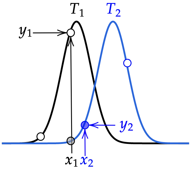
Figure 1: Task shift. A context observation $c_{1}=(x_{1},y_{1})$ is given for task $T_{1}$ (black line). Then, the task is changed to $T_{2}$ (blue line). After the task is shifted to $T_{2}$, the value $f(x_{2})$ is asked whose true value is $y_{2}$. A standard attention will use the out-dated $c_{1}=(x_{1},y_{1})$ to infer $f(x_{2})$ and a high attention-weight will be given to it because $x_{1}$ and $x_{2}$ are close each other. As a result, the attention will suggest a high value for $f(x_{2})$ while the true value $y_{2}$ is small. Our proposed model reconstructs $c_{1}$ so that its value can be properly adapted to the new task ($T_{2}$).

To this end, we propose a novel attention mechanism for meta-transfer learning, called Recurrent Memory Reconstruction and Attention (RMRA). In RMRA, to resolve the sparsity problem, for each task, we augment the context memory with generated imaginary context. Thus, even if a task provides a small or empty context, we can still apply attention effectively on the generated imaginary context. To resolve the obsolete context problem, we generate this imaginary context by a novel Recurrent Memory Reconstruction (RMR) mechanism. RMR temporally encodes all the past context observations using recurrent updates and then reconstructs a reformed imaginary context for each task. In this way, the past contexts are properly transformed to a useful representation for the current task. In addition, we do not need to limit the attention interval using a window but can use the entire past information without storing it explicitly. By augmenting the SNP model with RMRA, we propose a novel robust SNP model, called Attentive SNP (ASNP).

Our main contributions are: (i) we identify the problem why SNP should also suffer from underfitting and empirically show that it is indeed the case, (ii) we provide the reasons why existing attention mechanisms for NP is sub-optimal in the meta-transfer learning setting — due to sparse and obsolete context — and provide empirical analysis for it, (iii) we propose a novel Recurrent Memory Reconstruction and Attention (RMRA) mechanism to resolve the problem and also propose the ASNP model integrating RMRA into SNP, and (iv) in our experiments, we empirically show that the RMRA mechanism resolves the underfitting problem efficiently and effectively and provide superior performance to baseline models in various meta-transfer learning tasks.

2 Background

Neural Process (NP) (garnelo2018neural) learns to learn a task $\tau$ to map an input $x\in\mathbb{R}^{d_{x}}$ to an output $y\in\mathbb{R}^{d_{y}}$ given a context dataset $C=(X_{C},Y_{C})=\{(x^{(n)},y^{(n)})\}_{n\in[N_{C}]}$. Here, $N_{C}$ is the number of data points in $C$ and $[N_{C}]\equiv\{1,\ldots,N_{C}\}$. To learn a task distribution from this context, NP uses a distribution $P(z|C)$ to sample a task representation $z$. This makes NP a probabilistic meta-learning framework. Next, an observation model $p(y|x,z)$ takes an input $x$ and returns an output $y$. The generative process for NP conditioned on the context is given by:

$${P(Y,z|X,C)=P(Y|X,z)P(z|C)}$$ (1)

where $P(Y|X,z)=\prod_{n\in[N_{D}]}P(y^{(n)}|x^{(n)},z)$ and $D=(X,Y)=\{(x^{(n)},y^{(n)})\}_{n\in[N_{D}]}$ is the target dataset. To obtain the training data for this meta-learning setting, we draw multiple tasks from the true task distribution and sample $(C,D)$ for each task. Note that to implement NP, $C$ is encoded via a permutation-invariant function, such as $\sum_{n}\text{MLP}(x^{(n)},y^{(n)})$. anp argue that such a sum-aggregation produces an encoding that is not expressive enough and consequently hurts the observation model $P(Y|X,z)$. This is a key limitation of NP and is addressed by Attentive Neural Processes (ANP).

Attentive Neural Process (ANP)  anp identifies the problem of underfitting in NP. In underfitting, tasks learned from the context set fail to accurately predict the target points, including those in the context set. Also, the learned task distribution shows high uncertainty. To address this, using a larger latent $z$ is shown to be insufficient. To resolve this, ANP integrates the observation model $p(y|x,z)$ with attention on the context points. This allows the model to take a query $x$ and attend to the most relevant data points to predict the target output $y$. To achieve this, an attention function $\text{Attend}(C;x^{q})$ is implemented, which takes the context $C$ and a query $x^{q}$ and returns a read value $r_{x^{q}}$.

$${r_{x^{q}}=\text{Attend}(C;x^{q})=\sum_{n\in[N_{C}]}w_{n}y^{(n)}}$$ (2)

Here, for each $y^{(n)}\in Y_{C}$, there is an associated weight $w_{n}$ that is computed using a similarity function $\text{sim}(X_{C},x^{q})$. Using the read value, the observation model in ANP becomes $P(y|x,z,r_{x})$ and results in the following generative process.

$${P(y,z|x,C)=P(y|x,z,r_{x})P(z|C)}$$ (3)

where $(x,y)\in D$ is a target point. The ANP framework allows for the use of a variety of attentive mechanisms such as Dot-Product, Laplace, or Multi-Head attention (vaswani2017attention).

Sequential Neural Process (SNP) (snp) While the goal of meta-learning is to learn a single task distribution from a given context $C$, many situations consist of a sequence of tasks $\{\tau_{t}\}_{t\in[T]}$ whose distributions are correlated. Here, $t$ is a task-step. Thus, a framework that learns a task $\tau_{t}$ from a context $C_{t}$ must also utilize the correlation with the previous tasks to be able to learn with less context. Let $z_{t}$ denote a representation for a task $\tau_{t}$. Then SNP uses a distribution $p(z_{t}|z_{<t},C_{t})$ to learn from both $C_{t}$ and the previous task representations $z_{<t}$. From this viewpoint, SNP is a meta-transfer learning framework. Given task representation $z_{t}$, the model takes a query $x_{t}$ and generates an output $y_{t}$ through an observation model $p(y_{t}|x_{t},z_{t})$.

For a task $\tau_{t}$, let $C_{t}=\{(x_{t}^{(n)},y_{t}^{(n)})\}$ be the context and $(x_{t},y_{t})$ be a target point. With these, we describe the generative process for the target conditioned on the context as follows.

$${P(Y,Z|X,C)=\prod_{t=1}^{T}P(y_{t}|x_{t},z_{t})P(z_{t}|z_{<t},C_{t}).}$$ (4)

Here, $C$, $X$, $Y$ and $Z$ respectively denote the set aggregations of $C_{t}$, $x_{t}$, $y_{t}$ and $z_{t}$ over the entire roll-out.

3 Attentive Meta-Transfer

In this section, we describe our proposed model to resolve the problem of underfitting and using attention for its prevention in the setting of meta-transfer learning. We first propose a novel recurrent attention mechanism called Recurrent Memory Reconstruction (RMR), which resolves the problem of sparse context that makes underfitting more severe and obsolete context due to the task-shift problem which turns the past contexts to noise. Then, we propose to incorporate RMR into the SNP framework, yielding a robust meta-transfer learning model, Attentive Sequential Neural Processes (ASNP).

3.1 Recurrent Memory Reconstruction

Algorithm 1 Recurrent Memory Reconstruction

0:  $f_{xy}^{c}=$ MLP,   $f_{\text{order-invariant}}^{c}=\sum f_{xy}^{c}$

0:  $h_{0}^{x}$, $\{\tilde{h}_{0}^{k}\}_{k\in[K]}$, $\tilde{X}_{0}$, $\{\tilde{v}_{0}^{k}\}_{k\in[K]}$

  for $t\in[T]$ do

    # Context Processing

    $r_{t}^{c}\leftarrow f_{\text{order-invariant}}^{c}(C_{t})$

    $C_{t}\leftarrow\{(x_{t}^{(n)},f_{xy}^{c}(x_{t}^{(n)},y_{t}^{(n)})):(x_{t}^{(n)},y_{t}^{(n)})\in C_{t}\}$

    

    # Key Imagination

    $h_{t}^{x}\leftarrow\text{RNN}(\tilde{X}_{t-1},h_{t-1}^{x},r_{t}^{c})$

    $\tilde{X}_{t}\leftarrow f_{X}(h_{t}^{x})$

    

    # Value Imagination

    for $k\in[K]$ in parallel do

      $\tilde{h}_{t}^{(k)}\leftarrow\text{RNN}_{k}(\tilde{x}_{t}^{(k)},\tilde{v}_{t-1}^{(k)},\tilde{h}_{t-1}^{(k)})$

    end for

    $\{\tilde{v}_{t}^{(k)}\}_{k\in[K]}\leftarrow\text{Attend}(C_{t}\cup\{(\tilde{x}_{t}^{(k)},\tilde{h}_{t}^{(k)})\}_{k\in[K]};\tilde{X}_{t})$

    

    # Store

    $\tilde{C}_{t}\leftarrow\{(\tilde{x}_{t}^{(k)},\tilde{v}_{t}^{(k)})\}_{k\in[K]}$

  end for

To resolve the limitations of standard attention models to sparse context and obsolete context, we propose the Recurrent Memory Reconstruction (RMR) mechanism. The key ideas in RMR are (i) to generate imaginary context to complement the sparse context and (ii) to introduce recurrent reformation to appropriately transform the obsolete context to a new useful representation upon a task-shift. The imaginary context is constructed at each task-step on the updated representation of past contexts via recurrent reformation.

The main task of RMR at each task-step $t$ is to generate a new imaginary context $\tilde{C}_{t}$ from an encoding representation of the past contexts including both real and imaginary. The imaginary context contains $K$ memory cells, each of which is a key-value pair $(\tilde{x}_{t}^{(k)},\tilde{v}_{t}^{(k)})$ for $k\in[K]\equiv\{1,\dots,K\}$. We denote the imagined key-set by $\tilde{X}_{t}=\{\tilde{x}_{t}^{(k)}\}_{k}$ and the imagined value-set by $\tilde{V}_{t}=\{\tilde{v}_{t}^{(k)}\}_{k}$. When generating an imaginary context, we also use the real context $C_{t}$ gathered from the current task $\tau_{t}$ in order to inform the RMR about the characteristics of the current task. This is summarized by:

$${\tilde{C}_{t},\tilde{{\cal H}}_{t}=\text{RMR}(C_{t},\tilde{C}_{{t-1}},\tilde{{\cal H}}_{{t-1}})}$$ (5)

where $\tilde{{\cal H}}_{t}=\tilde{{\cal H}}_{t}^{\text{key}}\cup\tilde{{\cal H}}_{t}^{\text{val}}$ is a set of RMR’s hidden states, which consists of the hidden states of key generation and value generation, respectively. RMR generates imaginary keys first and then, conditioning on the generated keys, the imaginary values.

Figure 2: Illustration of Recurrent Memory Reconstruction (RMR) for generating imaginary context.

3.1.1 Generating Imaginary Keys

The main goal of imaginary key generation is to update the formation of the inputs (i.e., keys) upon a task-shift so that it can provide an attention on a meaningful area of the new task. As this requires to see (i) what input areas have covered so far, to learn the task-shift dynamics via $\tilde{X}_{{t-1}}$ and (ii) what is the current task via $C_{t}$, RMR deploys an RNN, called the key-tracker. Then, the key-generation process can be summarized by:

$${(\tilde{X}_{t},\tilde{h}_{t}^{\text{key}})=\text{GenerateKey}(C_{t},\tilde{X}_{{t-1}},\tilde{h}_{{t-1}}^{\text{key}}).}$$ (6)

where $\tilde{h}_{t}^{\text{key}}$ is the hidden state of the key-tracker.

Specifically, we first concatenate the previous imaginary-keys $\tilde{x}_{{t-1}}^{(1)},\dots,\tilde{x}_{{t-1}}^{(K)}$ to make the input representation and then encode the real context $C_{t}$ using an order-invariant encoder $r_{t}=\sum_{n}\text{MLP}(x_{t}^{(n)},y_{t}^{(n)})$. Then, the concatenated keys and real context encoding are provided to the key-tracker RNN as the inputs. The new imaginary key-set $\tilde{X}_{t}$ is generated from the updated hidden state $\tilde{h}_{t}^{\text{key}}$. For the order-invariant encoding, other implementation options may be found in (garnelo2018neural; eslami2018neural; gordon2019convolutional).

3.1.2 Generating Imaginary Values

Given new imaginary keys, we then need to generate the corresponding imaginary values. Similar to the key generation process, to generate a new value set $\tilde{V}_{t}$, RMR takes the new key $\tilde{X}_{t}$, the new real context $C_{t}$, and the previous value-set $\tilde{V}_{{t-1}}$ as inputs, resulting in the following summary interface:

$${\tilde{V}_{t},\tilde{H}_{t}^{\text{val}}=\text{GenerateValue}(\tilde{X}_{t},C_{t},\tilde{V}_{{t-1}},\tilde{H}_{{t-1}}^{\text{val}})}$$ (7)

where $\tilde{H}_{{t-1}}^{\text{val}}$ is a set of hidden states used for value generation.

In designing the value generator, we found two principles that play a key role. First, a value generation should be aware of what has happened in the past to generate a useful value for the current task upon a task-shift. Second, the values in a value-set should be aware of each other in order to obtain an optimal formation of the values. To realize this, we implement the value generation by the following two components: value-flow tracking and value-flow interaction.

i) Value-Flow Tracking. The purpose of this stage is to implement recurrence capturing value-transitions across tasks. To this end, for each memory cell $k\in[K]$, we assign an RNN, TrackValueFlow, which updates the value by:

$${\tilde{h}_{t}^{(k)}=\text{TrackValueFlow}(\tilde{x}_{t}^{(k)},\tilde{v}_{{t-1}}^{(k)},\tilde{h}_{{t-1}}^{(k)})}$$ (8)

where $\tilde{h}_{t}^{(k)}$ is the RNN hidden-state which we call the value-tracker state. Here, each value-tracker state acts as a proposal for the final imaginary value, and each RNN can be seen as tracking the flow of the value in a particular memory cell, hence the name.

ii) Value-Flow Interaction. After the update of TrackValueFlow, the values are updated upon the new key and its previous value. However, it does not know yet what other values are generated. To realize this interactive update, we revise the proposed values based on the correlations with other values in the value-set and the new context. Specifically, we first use the proposal values to construct a proposal key-value set $\tilde{C}^{\text{prop}}_{t}=\{(\tilde{x}_{t}^{(k)},\tilde{h}_{t}^{(k)}\}_{k\in[K]}$. We then combine it with the real context $C_{t}$ to get $C_{t}\cup\tilde{C}^{\text{prop}}_{t}$. Finally, we perform self-attention on this union using the imaginary keys as the attention query set and obtain the final imaginary value-set $\tilde{V}_{t}=\{\tilde{v}_{t}^{(k)}\}_{k\in[K]}$:

$${\tilde{V}_{t}=\text{Self-Attend}(C_{t}\cup\tilde{C}^{\text{prop}}_{t};\tilde{X}_{t}).}$$ (9)

This completes the generation of imaginary context, $\tilde{C}_{t}=(\tilde{X}_{t},\tilde{V}_{t})$. Algorithm 1 and Fig. 2 show the described process of generating imaginary context.

3.1.3 Reading in RMR

To perform a read operation on the RMR at a given task-step $t$, we propose performing attention on the extended context $\bar{C}_{t}=C_{t}\cup\tilde{C}_{t}$. Given a query input $x_{t}^{q}$, we thus obtain the read value as follows $r_{x_{t}^{q}}=\text{Attend}(\bar{C}_{t};x_{t}^{q})$.

3.2 Attentive Sequential Neural Processes

Using the imagined context obtained from RMR, we can now address the problems of sparse and obsolete context in SNP. In this section, we describe how we augment Sequential Neural Processes with RMR and, in doing so, propose Attentive Sequential Neural Processes.

3.2.1 Generative Process

To resolve the underfitting problem along with sparse and obsolete context, we equip the observation model in SNP with an augmented memory $\bar{C}_{t}$ provided by RMR. With this, the observation model becomes $P(y_{t}|x_{t},z_{t},\bar{C}_{t})$ (see Fig. 3). Then, given a target input $x_{t}$, the observation model reads $\bar{C}_{t}$ to obtain an attention encoding $r_{x_{t}}=\text{Attend}(\bar{C}_{t};x_{t})$.

In this way, by combining SNP with RMR, the generative process can be written as follows: $P(Y,Z,\tilde{C}|X,C)=$

$${\prod_{t=1}^{T}\underbrace{P(y_{t}|x_{t},z_{t},\bar{C}_{t})P(z_{t}|z_{<t},\bar{C}_{t})}_{\text{SNP with access to RMR}}\underbrace{P(\tilde{C}_{t}|\tilde{C}_{<t},C_{\leq t})}_{\text{RMR Update}}.}$$ (10)

We call this model Attentive Sequential Neural Process with RMR (ASNP-RMR).

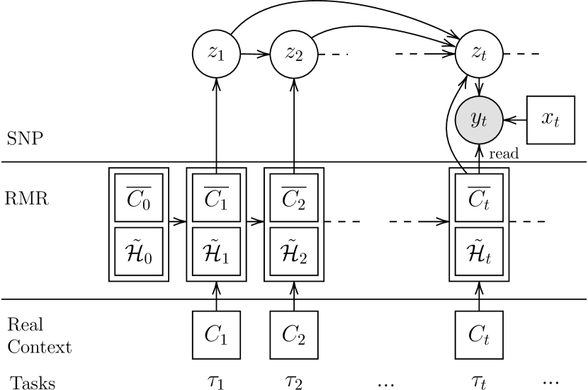
Figure 3: Illustration of the generative process of ASNP-RMR.

3.2.2 Learning and Inference

Due to the intractability of the true posterior, ASNP is trained via variational approximation with the following auto-regressive posterior approximation:

$${P(Z|\tilde{C},C,D)\approx\prod_{t=1}^{T}Q(z_{t}|z_{<t},\tilde{C}_{\leq t},C,D)}$$ (11)

where $D=(X,Y)$. For training, the following ELBO is maximized w.r.t. $\theta$ and $\phi$: ${\cal L}_{\text{ASNP}}(\theta,\phi)=$

$$\begin{aligned} &\sum_{t=1}^{T}\mathbb{E}_{Q_{\phi}(z_{t}|C,D)}\left[\log P_{\theta}(y_{t}|x_{t},z_{t},\tilde{C}_{t},C_{t})\right]\\ &-\mathbb{E}_{Q_{\phi}(z_{<t})}\left[\mathbb{K}\mathbb{L}(Q_{\phi}(z_{t}|z_{<t},\tilde{C}_{\leq t},C,D)\parallel\right.\\ &\left.\quad\quad P_{\theta}(z_{t}|z_{<t},\tilde{C}_{\leq t},C_{\leq t}))\right].\end{aligned}$$

For backpropagation, we use the reparameterization trick (vae). See Appendix LABEL:app:elbo_deri for derivation.

4 Related Works

Meta-learning approaches have become attractive for learning to learn new tasks at test-time. In this line of work, GQN (eslami2018neural) renders 3D scenes from a few viewpoints, and NP (garnelo2018neural) generalizes GQN. Subsequently, ANP (anp) identifies and resolves the problem of underfitting in NP by using query-dependent representation. Similarly, in rosenbaum2018learning, the authors introduce attention to GQN to render complex 3D scenes in large procedurally-generated maps as in Minecraft. Functional Neural Processes (FNP) (louizos2019functional) learns a graph of dependencies between a pre-selected set of points and the training points for modeling distributions over functions. ANP-RNN (qin2019recurrent) encodes the target inputs via an RNN and use the hidden states as queries to attend on the context points in a meta-learning setting. To extend NP to meta-transfer learning, SNP (snp) models a sequence of tasks with sequential latent representations. It outperforms NP in meta-transfer learning a sequence of tasks that come from different but related distributions. Recurrent Neural Process (RNP) (kumar2019spatiotemporal) also deals with meta-transfer learning, but it transfers via deterministic representations and shows high uncertainty with sparse context. willi2019recurrent also proposes a model named RNP for meta-transfer learning.

The term meta-transfer learning has also been used in connection to a different set of problems that deal with discovery of causal mechanisms (bengio2019meta), fast-adaption from a large-scale trained model (sun2019meta), and knowledge transfer to different architectures and tasks (jang2019learning). In kang2018transferable, the authors propose transferable meta-learning to apply a meta-trained model to a task from a task distribution different from the trained.

santoro2018relational and goyal2019recurrent propose approaches combining self-attention and recurrent update. Recurrent Memory Core (RMC) (santoro2018relational) self-attends the entire memory with a single input vector and updates the memory through an RNN module. Recurrent Independent Mechanisms (RIM) (goyal2019recurrent) recurrently updates the memory but self-attends only the memories that are estimated to be the most relevant using the visual input. Although these methods combine recurrence and attention modules, however unlike RMR, their memory elements and inputs contain only values. They do not deal with key-value pairs in a meta-transfer learning setting.

5 Experiments

In this section, we describe our experiments to answer two key questions: i) By resolving the problems of sparse context and obsolete context, can we improve meta-transfer learning? ii) If yes, what are the needed memory sizes and computational overhead during training? We also perform an ablation on RMR to demonstrate the need for flow-tracking and flow-interaction. In the rest of this section, we first describe the baselines and our experiment settings. We then describe our results on dynamic 1D regression, dynamic 2D image completion, and dynamic 2D image rendering.

	ANP	SNP	ASNP-W	ASNP-RMR
Sequential Latent	✗	✓	✓	✓
Attention	✓	✗	✓	✓
Recurrent Memory	✗	✗	✗	✓

Table 1: Taxonomy of the models considered for evaluation.

Baselines. We consider three baselines – ANP, SNP and ASNP-W. These are characterized by whether or not they contain a sequential latent, attention mechanism or a recurrent memory (see Table 1). Among these, ASNP-W is an extension of SNP such that the observation model attends on a window of $K$-most recent contexts. Hence, ASNP-W contains sequential latent and attention but not a recurrent memory. These baselines are to test whether sequential latent and standard attention alone can solve underfitting without addressing the problems of sparse and obsolete context. We also test ANP and SNP using different latent sizes to investigate its effect on performance. Similarly, we test ASNP-RMR and ASNP-W using different memory sizes and analyze its effect. See Appendix LABEL:app:model_details for more details on their implementation.

Figure 4: Top: Target-NLL computed at each time-step in the task sequence. Bottom: Target-NLL convergence against the wall-clock time computed during training on a held-out set. Hidden unit size in all models is $128$.

Performance Metric and Context Regimes. We evaluate our models on hundreds of held-out sequences of tasks and analyze their performance in modeling the target outputs. Our performance metric is Target-NLL defined as $-\mathbb{E}_{z\sim P(Z|C)}\log P(Y|X,Z,C)$. For dynamic 1D regression and dynamic 2D image completion, we consider two regimes for evaluation – i) Sparse-Context Regime. In this regime, we consider task-sequences of length $50$. We provide a sparse context for $45$ randomly chosen tasks and empty context for the remaining. This regime tests the model’s ability to transfer-learn from sparse contexts gathered from different tasks. At every increment of the task-step, we expect the model’s performance to improve as the model collects more context. ii) Transfer-Prediction Regime. In this regime, we consider task-sequences of length $20$. We provide a large-sized context for the first $10$ task-steps and empty context for the remaining. This regime allows the model to infer the first $10$ tasks and their dynamics with high certainty. Subsequently, the model must use this information to transfer-learn the remaining $10$ tasks. At every increment of the task-step, we expect the performance of any model to deteriorate as the contexts become more obsolete. However, if a model can deal with this problem, we expect it to show less degradation.

For 2D dynamic image rendering also, we experiment on the sparse-context and transfer-prediction regimes but with task-sequences of length $6$. See Appendix LABEL:app:task_details for details about sequence lengths and context sizes.

5.1 Dynamic 1D Regression

In this setting, the tasks are 1D functions that change with time. To generate this dataset, we draw a function from a GP at each task-step such that the kernel-parameters of the GP change according to some linear dynamics. Hence, the model must estimate the function at unseen points and also track the shifts in its shape. In our experiments, the GPs use a squared-exponential kernel. See Appendix LABEL:app:gp_details for more details.

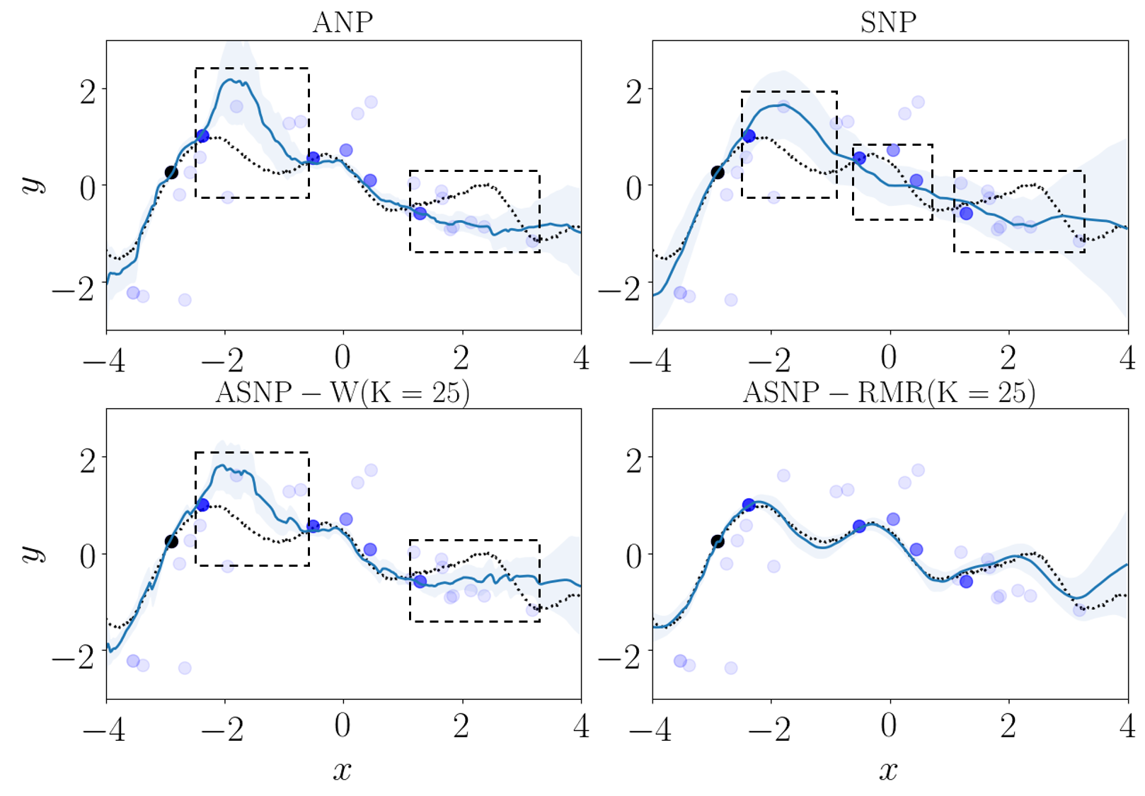
Figure 5: Samples for dynamic 1D regression in sparse-context regime at $t=33$. Dotted line: True function. Blue line: Predicted function. Shaded light-blue region: Uncertainty. Black dot: Context points at $t=33$. Blue dots: Past context points. Darker dots are more recent. Dashed-rectangles: Regions where the predictions are inaccurate.

Figure 6: Target-NLL computed as a function of memory sizes in sparse-context regime. Here, $h$ denotes the latent size.

Figure 7: Target-NLL computed at each time-step in moving CelebA image completion task sequence. Hidden unit size in all models is $128$.

Target-NLL. We plot the target-NLLs for each task-step in Fig. 4. Consider the performance of ASNP-W to study the effect of extending SNP with standard attention. We observe that improvements compared to SNP are small. Comparing these with ASNP-RMR shows that sequential latent and standard attention alone cannot solve underfitting without addressing sparse and obsolete contexts. In transfer-prediction regime, for $t\leq 10$, we note that target-NLLs of ANP are similar to that of ASNP-RMR. This is because, in this interval, ANP exploits the larger context sizes without attending to the obsolete points. However, the main focus of this setting is multi-step transfer for $t>10$ on which ANP degrades quickly.

Effect of Memory Size and Latent Size. In Fig. 6, we show the effect of memory and latent sizes on performance. We observe that increasing the latent size in SNP from $128\text{ to }1024$ yields small improvements with diminishing returns. This shows that a larger latent size is not adequate. Additionally, we observe that ASNP-W does not surpass ANP significantly. Hence, we conclude that the recurrent latents $z_{\leq t}$ fails to inform the observation model about the shift in the obsolete points. We further note that ASNP-RMR at $K=9$ outperforms ASNP-W for all choices of $K$. This demonstrates better size-efficiency of RMR.

Training Time. In Fig. 4, we plot the target-NLL against the training wall-clock time, and we note that ASNP-RMR imposes no significant overhead in convergence.

Qualitative Analysis. In Fig. 5, we show the predictive means of the target function. We observe that SNP underfits the target function in multiple locations. Furthermore, in ANP and ASNP-W, attention helps the prediction only at those obsolete points that did not undergo a significant shift. In these models, attention also causes misestimation of the function when obsolete points shift significantly. It shows that without addressing the obsolete context issue, the standard attention cannot resolve underfitting. In contrast, ASNP-RMR yields more accurate predictions.

5.2 Dynamic 2D Image Completion

In this setting, the task is to complete an image by estimating a pixel value at a given pixel location. The image belongs to a sequence of images that contains a moving image patch on a white canvas. In this dynamic setting, the model must not only estimate the unseen pixel values but also track their motion. The moving images are taken from the MNIST (lecun1998gradient) and CelebA (liu2015faceattributes) datasets, and hence we call these settings moving MNIST and moving CelebA, respectively.

Target NLL. We plot the target-NLLs in Fig. 7. Recall that in the sparse-context regime, a model must transfer-learn at every task-step, and in the transfer-prediction regime, a model must transfer-learn on task-steps $t>10$ that have an empty context. We observe that when such transfer-learning is required, the performance of ASNP-W degrades compared to SNP. This implies that attention on obsolete points is not only ineffective but also detrimental.

Effect of Memory and Latent Sizes. From Fig. 6, our conclusions about the effect of memory size and latent size are similar to those in dynamic 1D regression. ASNP-RMR is not only size-efficient but also shows monotonic improvement as we increase the memory size. Note that in Fig. 6, we do not test ANP using a larger latent size because we found its memory usage too large to train.

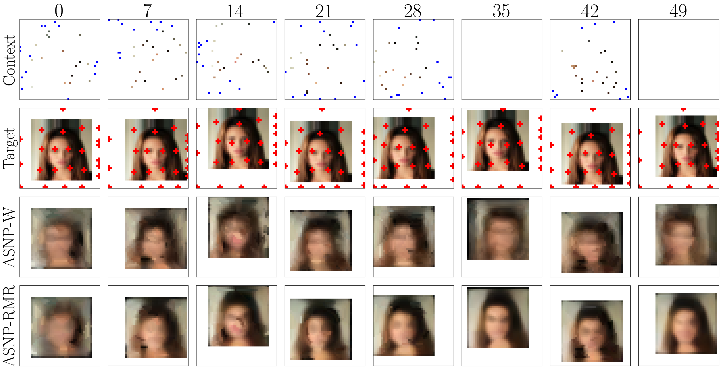
Figure 8: Qualitative evaluation on moving CelebA image completion task sequence. Red dots: Imaginary keys imagined by ASNP-RMR. The memory size $K$ is $25$.

Qualitative Analysis. Fig. 8 shows the positions of imaginary keys generated by RMR. We observe that the model learns to discover certain key points on the CelebA patch, and it tracks them as the patch moves. It also places some keys on the edges of the canvas to account for the bounces. Fig. 9 shows qualitative samples for moving MNIST image completion in sparse-context setting. As ASNP-RMR accumulates more context, RMR reforms the obsolete points for the current task. Consequently, we observe that the predicted images become clearer over time. We also observe that in contrast to SNP, ASNP-W shows deterioration. In Fig. 9 and Fig. 8, consider the task-steps with an empty context. We note that on these task-steps, ANP and ASNP-W predict poor quality images compared to ASNP-RMR, showing that standard attention is unable to deal with the obsolete context.

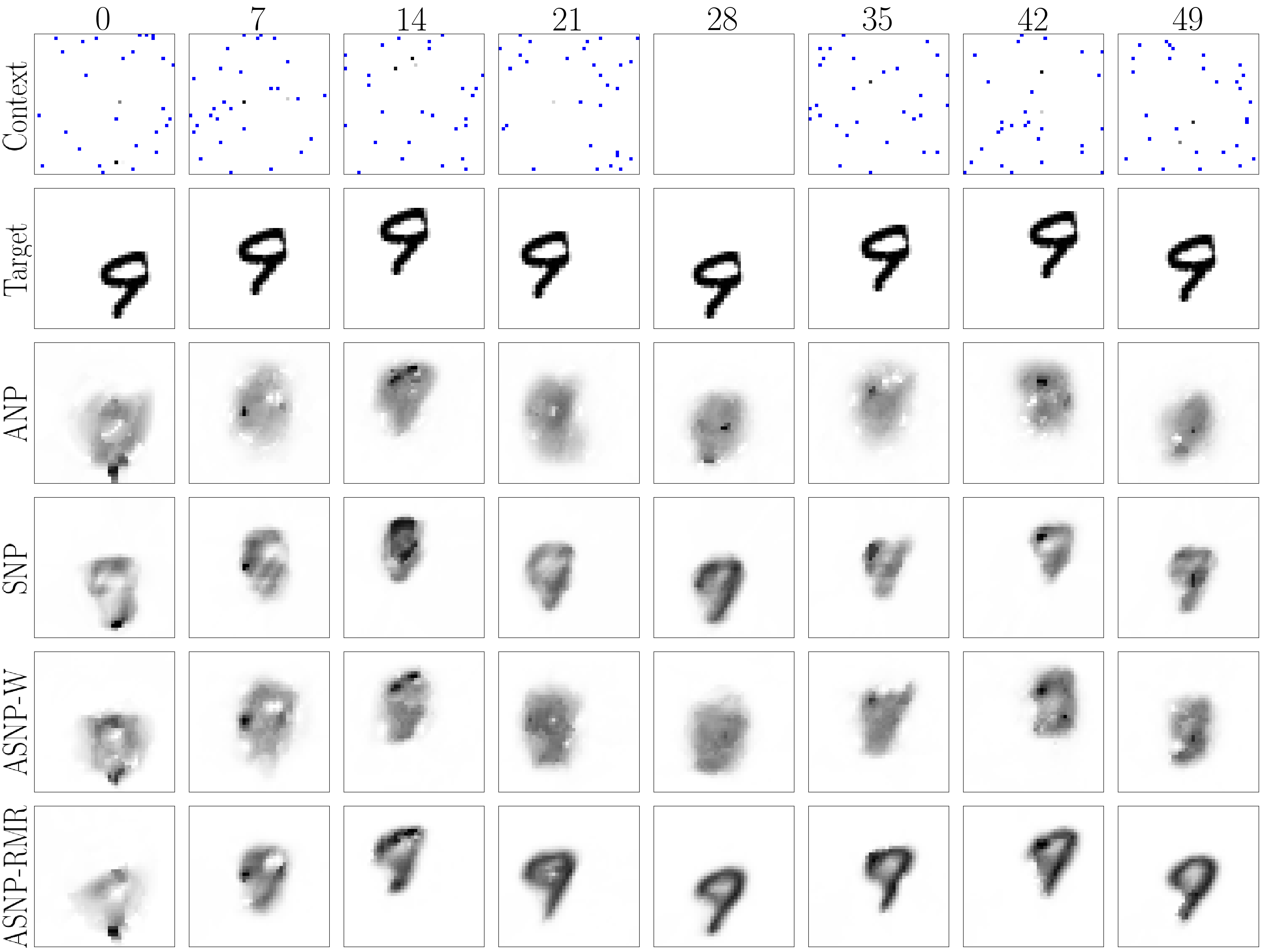
Figure 9: Moving MNIST image completion samples in the sparse-context regime. Memory size of ASNP-RMR is $25$.

5.3 Ablation Study on RMR

In this section, we perform an ablation on RMR to create two modifications, and we report the results in Fig. 10.

i) No Value-Flow Tracking. In this modification, the model generates new imaginary values only via self-attention on the previous values. Thus, without the recurrence, we expect the model to forget the transition dynamics. In Fig. 10, we observe in the transfer-prediction setting that the performance deteriorates severely in task-steps $[11,20]$. This is because the context is empty, and value imagination fails to extrapolate without capturing the transition dynamics.

ii) No Value-Flow Interaction. In this modification, the model generates new imaginary values only via Value-Flow Tracking. To incorporate the real context, we provide it as an input to the flow tracking RNNs. Because the values do not interact, we observe performance degradation in Fig. 10. Thus, we conclude that to perform effective value imagination, the model requires both flow tracking and flow interaction.

5.4 Dynamic 2D Image Rendering

In this setting, we consider a sequence of images as in the moving CelebA dataset. The task for the model is to take a location on the canvas and predict the image-patch centered at the location. Because the task is to generate an image, we replace the SNP baseline with a TGQN (snp). Similarly, we replace ASNP-RMR and ASNP-W with ATGQN-RMR and ATGQN-W, respectively. Here, ATGQN stands for attentive TGQN – a model that we develop by incorporating attention into TGQN. Hence, ATGQN-RMR is TGQN equipped with attention on RMR, and ATGQN-W is equipped with standard attention on a context window. See Appendix LABEL:app:rendering_details for implementation details. We report the results on these models in Table 2, and we note that ATGQN-RMR outperforms ATGQN-W and TGQN.

Figure 10: Target-NLL for ASNP-RMR compared against two alternate versions by way of ablation – i) without flow-tracking and ii) without flow-interaction.

Regime	ATGQN -RMR	ATGQN -W	TGQN
Sparse-Context	2.57	2.77	3.23
Transfer-Prediction	2.04	2.8	3.08

Table 2: Target-NLL comparison between ATGQN-RMR, ATGQN-W and TGQN in moving CelebA image rendering task.

6 Conclusion

In this paper, we argued that the two problems, sparse context and obsolete context, observed in meta-transfer learning due to temporal task-shift, make the underfitting issue in SNP more severe. Then, to resolve this problem, we proposed a novel attention model using imaginary context generated by Recurrent Memory Reconstruction (RMR) and a robust probabilistic meta-transfer learning model, Attentive Sequential Neural Processes. Our experiments demonstrate that existing methods show weaknesses upon a sparse and obsolete context, and that using RMR-based attention in SNP is an effective way to resolve the issue. The ablation study shows that the recurrent context modeling and the interaction model are the key components to achieve this improved robustness. In the future, it will be interesting to apply this robust model to various other problems including meta-transfer reinforcement learning.