Reconstructing Biological and Digital Phylogenetic Trees in Parallel

Abstract

In this paper, we study the parallel query complexity of reconstructing biological and digital phylogenetic trees from simple queries involving their nodes. This is motivated from computational biology, data protection, and computer security settings, which can be abstracted in terms of two parties, a responder, Alice, who must correctly answer queries of a given type regarding a degree-$d$ tree, $T$, and a querier, Bob, who issues batches of queries, with each query in a batch being independent of the others, so as to eventually infer the structure of $T$. We show that a querier can efficiently reconstruct an $n$-node degree-$d$ tree, $T$, with a logarithmic number of rounds and quasilinear number of queries, with high probability, for various types of queries, including relative-distance queries and path queries. Our results are all asymptotically optimal and improve the asymptotic (sequential) query complexity for one of the problems we study. Moreover, through an experimental analysis using both real-world and synthetic data, we provide empirical evidence that our algorithms provide significant parallel speedups while also improving the total query complexities for the problems we study.

1 Introduction

Phylogenetic trees represent evolutionary relationships among a group of objects. For instance, each node in a biological phylogenetic tree represents a biological entity, such as a species, bacteria, or virus, and the branching represents how the entities are believed to have evolved from common ancestors [28, 7, 33]. (See Figure 1(a).) In a digital phylogenetic tree, on the other hand, each node represents a data object, such as a computer virus [21, 34], a source-code file [26], a text file or document [31, 39], or a multimedia object (such as an image or video) [5, 15, 14, 13] and the branching represents how these objects are believed to have evolved through edits or data compression/corruption. (See Figure 1(b).)

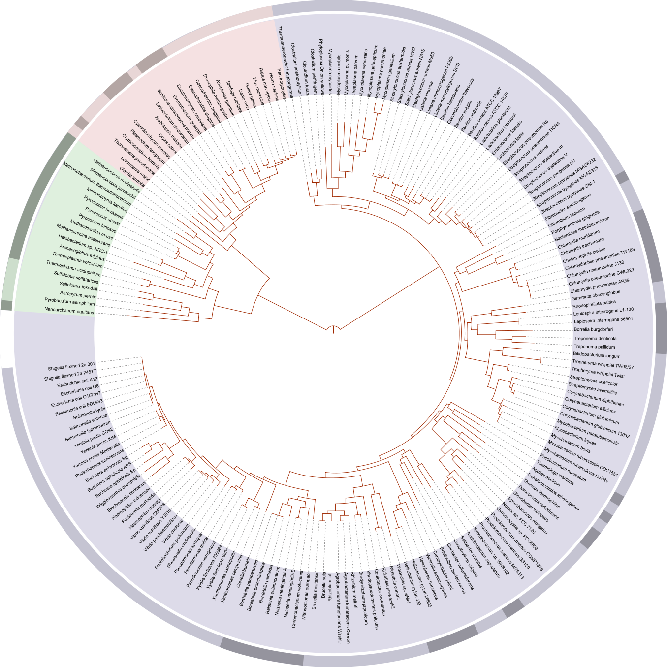
(a)

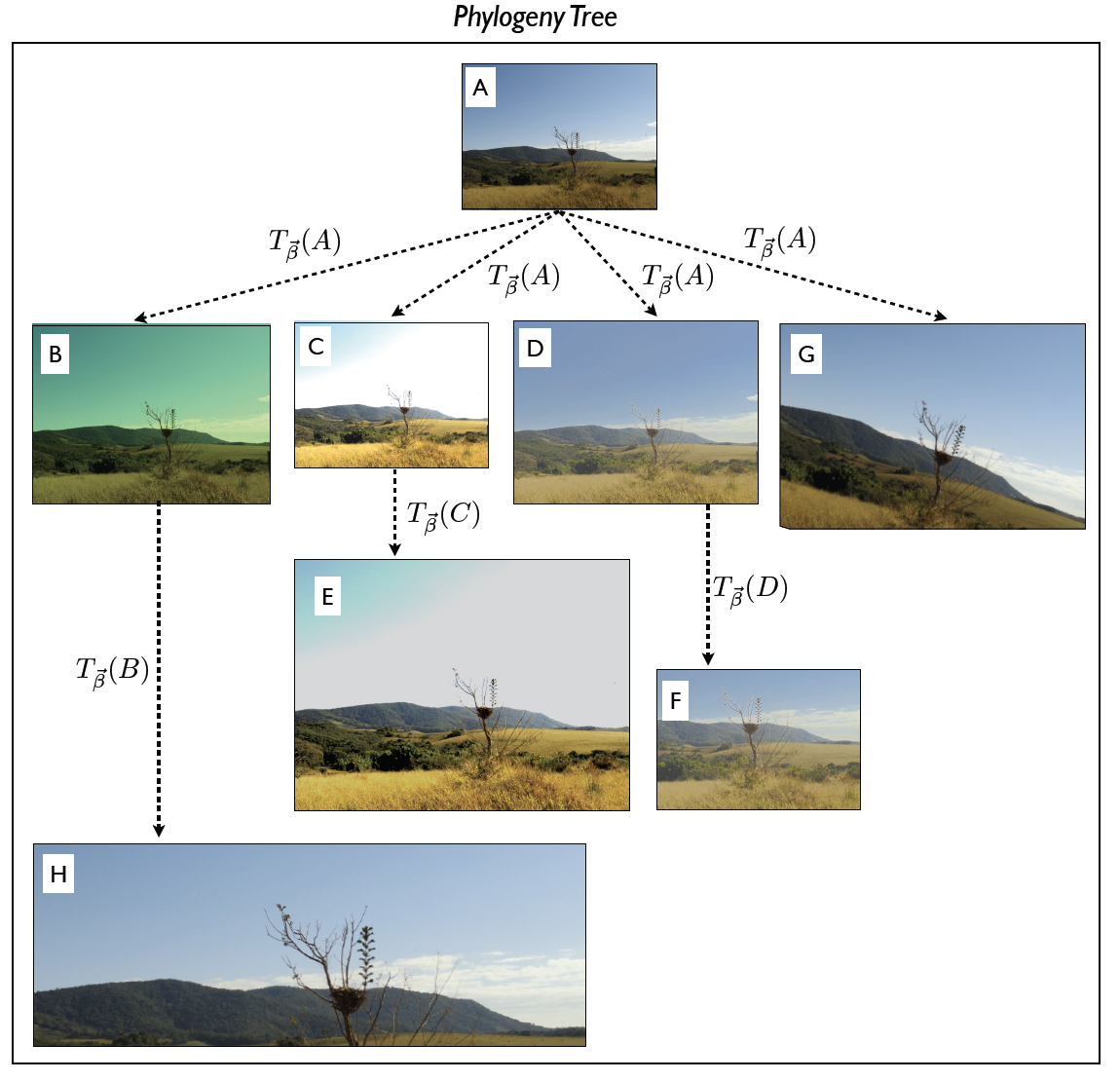
(b)

Figure 1: Two phylogenetic trees. (a) A biological phylogenetic tree of life, showing relationships between species whose genomes had been sequenced as of 2006; public domain image by Ivica Letunic, retraced by Mariana Ruiz Villarreal. (b) A digital phylogenetic tree of images, from Dias et al. [13].

In this paper, we are interested in studying efficient methods for reconstructing phylogenetic trees from queries regarding their structure, noting that there are differences in the types of queries one may perform on the two types of phylogenetic trees. In particular, with some exceptions, in a biological phylogenetic tree we can only perform queries involving the leaves of the tree, since these typically represent living biological entities and internal nodes represent ancestors that are likely to be extinct. In digital phylogenetic trees, on the other hand, we can perform queries involving any of the nodes in the tree, including internal nodes, since these represent digital artifacts, which are often archived. The former type of phylogenetic tree has also received attention in the context of hierarchical clustering, where the goal is to provide a hierarchical grouping structure of items according to their similarity [17]. To support reconstruction of both biological and digital phylogenetic trees, therefore, we study both types of querying regimes in this paper.

More specifically, with respect to biological phylogenetic trees, we focus on relative-distance queries, where one is given three leaf nodes (corresponding to species), $x$, $y$, and $z$, and the response is a determination of which pair, $(x,y)$, $(x,z)$, or $(y,z)$, is a closest pair, hence, has the most-recent common ancestor [28]. With respect to digital phylogenetic trees, we instead focus on path queries, where one is given two nodes, $v$ and $w$, in the tree and the response is “true” if and only if $v$ is an ancestor of $w$.

The motivation for reconstructing phylogenetic trees comes from a desire to better understand the evolution of the objects represented in a given phylogenetic tree. For example, understanding how biological species evolved is useful for understanding and categorizing the fossil record and understanding when species are close relatives [28, 17]. Similarly, understanding how digital objects have been edited and transformed can be useful for data protection, computer security, privacy, copyright disputes, and plariarism detection [21, 34, 26, 31, 39, 5, 15, 14, 13]. For instance, understanding the evolutionary process of a computer virus can provide insights into its ancestry, characteristics of the attacker, and where future attacks might come from and what they might look like [34].

The efficiency of a tree reconstruction algorithm can be characterized in terms of its query-complexity measure, $Q(n)$, which is the total number of queries of a certain type needed to reconstruct a given tree. This parameter comes from machine-learning and complexity theory, e.g., see [1, 8, 16, 41], where it is also known as “decision-tree complexity,” e.g., see [47, 4]. Previous work on tree reconstruction has focused on sequential methods, where queries are issued and answered one at a time. For example, in pioneering work for this research area, Kannan et al. [28] show that an $n$-node biological phylogenetic tree can be reconstructed sequentially from $O(n\log n)$ three-node relative-distance queries.

Indeed, their reconstruction algorithms are inherently sequential and involve incrementally inserting leaf nodes into the phylogenetic tree reconstructed for the previously-inserted nodes.

In many tree reconstruction applications, queries are expensive [28, 17, 21, 34, 26, 31, 39, 5, 15, 14, 13], but can be issued in batches. For example, there is nothing preventing the biological experiments [28] that are represented in three-node relative-distance queries from being issued in parallel. Thus, in order to speed up tree reconstruction, in this paper we are interested in parallel tree reconstruction. To this end, we also use a round-complexity parameter, $R(n)$, which measures the number of rounds of queries needed to reconstruct a tree such that the queries issued in any round comprise a batch of independent queries. That is, no query issued in a given round can depend on the outcome of another query issued in that round, although both can depend on answers to queries issued in previous rounds. Roughly speaking, $R(n)$ corresponds to the span of a parallel reconstruction algorithm and $Q(n)$ corresponds to its work. In this paper, we are interested in studying complexities for $R(n)$ and $Q(n)$ with respect to biological and digital phylogenetic trees with fixed maximum degree, $d$.

1.1 Related Work

The general problem of reconstructing graphs from distance queries was studied by Kannan et al. [29], who provide a randomized algorithm for reconstructing a graph of $n$ vertices using $\tilde{O}(n^{3/2})$ distance queries.

Previous parallel work has focused on inferring phylogenetic trees through Bayesian estimation [3]. However, we are not aware of previous parallel work using a similar query models to ours. With respect to previous work on sequential tree reconstruction, Culberson and Rudnicki [12] provide the first sub-quadratic algorithms for reconstructing a weighted undirected tree with $n$ vertices and bounded degree $d$ from additive queries, where each query returns the sum of the weights of the edges of the path between a given pair of vertices. Reyzin and Srivastava [37] show that the Culberson-Rudnicki algorithm uses $O(n^{3/2}\cdot\sqrt{d})$ queries.

Waterman et al. [46] introduce the problem of reconstructing biological phylogenetic trees, using additive queries, which are more powerful than relative-distance queries. Hein [23] shows that this problem has a solution that uses $O(dn\log_{d}n)$ additive queries, when the tree has maximum degree $d$, which is asymptotically optimal [30]. Kannan et al. [28] show that an $n$-node binary phylogenetic tree can be reconstructed from $O(n\log n)$ three-node relative-distance queries. Their method appears inherently sequential, however, as it is based on an incremental approach that mimics insertion-sort. Similarly, Emamjomeh-Zadeh and Kempe [17] also give a sequential method using relative-distance queries that has a query complexity of $O(n\log n)$. Their algorithm, however, was designed for a different context, namely, hierarchical clustering.

Additionally, there exists some work (e.g. [27, 6, 24]) in an alternative perspective of the problem reconstructing phylogenetic trees, in which the goal is to find the best tree explaining the similarity and the relationship between a given fixed (or dynamic) set of data sequences (e.g. of species), using Maximum Parsimony [18, 20, 38] or Maximum Likelihood [19, 9]. This contrasts with our approach of recovering the “ground truth” tree known only to an oracle, which is consistent with its answers about the tree.

With respect to digital phylogenetic tree reconstruction, there are a number of sequential algorithms with $O(n^{2})$ query complexities, including the use of what we are calling path queries, where the queries are also individually expensive, e.g., see [21, 34, 26, 31, 39, 5, 15, 14, 13]. Jagadish and Sen [25] consider reconstructing undirected unweighted degree-$d$ trees, giving a deterministic algorithm that requires $O(dn^{1.5}\log n)$ separator queries, which answer if a vertex lies on the path between two vertices. They also give a randomized algorithm using an expected $O(d^{2}n\log^{2}n)$ number of separator queries, and they give an $\Omega(dn)$ lower bound for any deterministic algorithm. Wang and Honorio [45] consider the problem of reconstructing bounded-degree rooted trees, giving a randomized algorithm that uses expected $O(dn\log^{2}n)$ path queries. They also prove that any randomized algorithm requires $\Omega(n\log n)$ path queries.

Our Contributions.  In this paper, we study the parallel phylogenetic tree reconstruction problem with respect to the two different types of queries mentioned above:

• We show that an $n$-node rooted biological (binary) phylogenetic tree can be reconstructed from three-node relative-distance queries with $R(n)$ that is $O(\log n)$ and $Q(n)$ that is $O(n\log n)$, with high probability (w.h.p.). Both bounds are asymptotically optimal.

• We show that an $n$-node fixed-degree digital phylogenetic tree can be reconstructed from path queries, which ask whether a given node, $u$, is an ancestor of a given node, $w$, with $R(n)$ that is $O(\log n)$ and $Q(n)$ that is $O(n\log n)$, w.h.p. We also provide an $\Omega(dn+n\log n)$ lower bound for any randomized or deterministic algorithm suggesting that our algorithm is optimal in terms of query complexity and round complexity. Further, this asymptotically-optimal $Q(n)$ bound actually improves the sequential complexity for this problem, as the previous best bound for $Q(n)$, due to Wang and Honorio [45], had a $Q(n)$ bound of $O(n\log^{2}n)$ for reconstructing fixed-degree rooted trees using path queries. Of course, our method also applies to biological phylogenetic trees that support path queries.

A preliminary announcement of some of this paper’s results, restricted to binary trees, was presented in [2]. Most of our algorithms are quite simple, although their analyses are at times nontrivial. Moreover, given the many applications of biological and digital phylogenetic tree reconstruction, we feel that our algorithms have real-world applications. Thus, we have done an extensive experimental analysis of our algorithms, using both real-world and synthetic data for biological and digital phylogenetic trees. Our experimental results provide empirical evidence that our methods achieve significant parallel speedups while also providing improved query complexities in practice.

2 Preliminaries

In graph theory, an arborescence is a directed graph, $T$, with a distinguished vertex, $r$, called the root, such that, for any vertex $v$ in $T$ that is not the root, there is exactly one path from $r$ to $v$, e.g., see Tutte [42]. That is, an arborescence is a graph-theoretic way of describing a rooted tree, so that all the edges are going away from the root. In this paper, when we refer to a “rooted tree” it should be understood formally to be an arborescence.

We represent a rooted tree as $T=(V,E,r)$, with a vertex set $V$, edge set $E$, and root $r\in V$. The degree of a vertex in such a tree is the sum of its in-degree and out-degree, and the degree of a tree, $T$, is the maximum degree of all vertices in $T$. So, an arborescence representing a binary tree would have degree 3. Because of the motivating applications, e.g., from computational biology, we assume in this paper that the trees we want to reconstruct have maximum degree that is bounded by a fixed constant, $d$.

Let us review a few terms regarding rooted trees.

Definition 2.1.

(ancestry) Given a rooted tree, $T=(V,E,r)$, we say $u$ is parent of $v$ (and $v$ is a child of $u$) if there exists a directed edge $(u,v)$ in $E$. The ancestor relation is the transitive closure of the parent relation, and the descendant relation is the transitive closure of the child relation. We denote the number of descendants of vertex $s$ by $D(s)$. A node without any children is called a leaf. Given two leaf nodes, $u$ and $v$ in $T$, their lowest common ancestor, $lca(u,v)$, is the node, $w$ in $T$, that is an ancestor of both $u$ and $v$ and has no child that is also an ancestor of $u$ and $v$.

We next define the types of queries we consider in this paper for reconstructing a rooted tree, $T=(V,E,r)$.

Definition 2.2.

A relative-distance query for $T$ is a function, $closer$, which takes three leaf nodes, $u$, $v$, and $w$ in $T$, as input and returns the pair of nodes from the set, $\{u,v,w\}$, that has the lower lowest common ancestor. That is, $closer(u,v,w)=(u,v)$ if $lca(u,v)$ is a descendant of $lca(u,w)=lca(v,w)$. Likewise, we also have that $closer(u,v,w)=(u,w)$ if $lca(u,w)$ is a descendant of $lca(u,v)=lca(v,w)$, and $closer(u,v,w)=(v,w)$ if $lca(v,w)$ is a descendant of $lca(u,v)=lca(u,w)$.

Definition 2.2 assumes $T$ is a binary tree (of degree $3$). Note that in this paper we restrict relative-distance queries to leaves, since these represent, e.g., current species in the application of reconstructing biological phylogenetic trees.

Definition 2.3.

A path query for $T$ is a function, $path$, that takes two nodes, $u$ and $v$ in $T$, as input and returns $1$ if there is a (directed) path from vertex $u$ to $v$, and otherwise returns $0$. Also, for $u\in V$ and $W\subseteq V$, we define $count(u,W)=\sum_{v\in W}path(u,v)$, which is the number of descendants of $u$ in $W$.

We next study some preliminaries involving the structure of degree-$d$ rooted trees that will prove useful for our parallel algorithms.

Definition 2.4.

Let $T=(V,E,r)$ be a degree-$d$ rooted tree. We say that an edge $e=(x,y)\in E$ is an even-edge-separator if removing $e$ from $T$ partitions it into two rooted trees, $T^{\prime}=(V^{\prime},E^{\prime},y)$ and $T^{\prime\prime}=(V^{\prime\prime},E^{\prime\prime},r)$, such that $\frac{|V|}{d}\leq|V^{\prime}|\leq\frac{|V|(d-1)}{d}$ and $\frac{|V|}{d}\leq|V^{\prime\prime}|\leq\frac{|V|(d-1)}{d}$. (See Figure 2.)

Lemma 2.5.

Every rooted tree of degree-$d$ has an even-edge-separator.

Proof 2.6.

This follows from a result by Valiant [44, Lemma 2].

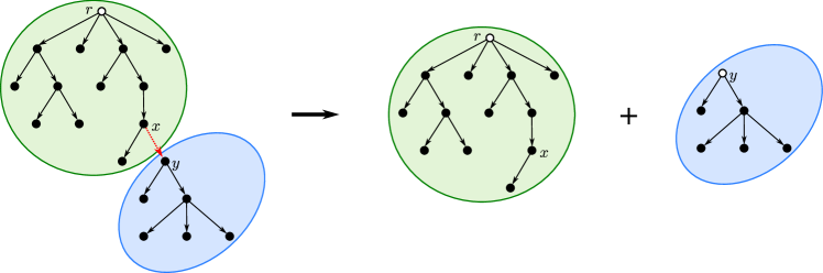
Figure 2: Illustration of a divide-conquer approach for trees. The edge $(x,y)$ is an even-edge-separator. Note that the root of $T^{\prime\prime}$ is $r$, while $y$ becomes root of $T^{\prime}$.

As we will see, this fact is useful for designing simple parallel divide-and-conquer algorithms. Namely, if we can find an even-edge-separator, then we can cut the tree in two by removing that edge and recurse on the two remaining subtrees in parallel (see Figure 2).

3 Reconstructing Biological Phylogenetic Trees in Parallel

Relative-distance queries model an experimental approach to constructing a biological phylogenetic tree, e.g., where DNA sequences are compared to determine which samples are the most similar [28]. In simple terms, pairs of DNA sequences that are closer to one another than to a third sequence are assumed to be from two species with a common ancestor that is more recent than the common ancestor of all three. In this section, for the sake of tree reconstruction, we assume the responder has knowledge of the absolute structure of a rooted binary phylogenetic tree; hence, each response to a $closer(u,v,w)$ query is assumed accurate with respect to an unknown rooted binary tree, $T$. As in the pioneering work of Kannan et al. [28], we assume the distance comparisons are accurate and consistent. The novel dimension here is that we consider parallel algorithms for phylogenetic tree reconstruction.

As mentioned above, we consider relative-distance queries to occur between leaves of a rooted binary tree, $T$. That is, in our query model, the querier has no knowledge of the internal nodes of $T$ and can only perform queries using leaves. Because $T$ is a binary phylogenetic tree, we may assume it is a proper binary tree, where each internal node in $T$ has exactly two children.

3.1 Algorithm

At a high level, our parallel reconstruction algorithm (detailed in Algorithm 1) uses a randomized divide-and-conquer approach, similar to Figure 2. In our case, however, the division process is random three-way split through a vertex separator, rather than an edge-separator-based binary split. Initially, all leaves belong to a single partition, $L$. Then two leaves, $a$ and $b$, are chosen uniformly at random from $L$ and each remaining leaf, $c$, is queried in parallel against them using relative-distance queries. Notice that the lowest common ancestor of $a$ and $b$ splits the tree into three parts. Given $a$ and $b$, the other leaves are split into three subsets ($R$, $A$, and $B$) according to their query result (as shown in Figure 3(a)):

• $A$: leaves close to $a$, i.e., for which $closer(a,b,c)=(a,c)$

• $B$: leaves close to $b$, i.e., for which $closer(a,b,c)=(b,c)$

• $R$: remaining leaves, i.e., for which $closer(a,b,c)=(a,b)$

Figure 3: (a) The subgroups leaves are split into. (b) The linking step attaching $T_{a}$, $T_{b}$ and $T_{r}$.

We then recursively construct the trees in parallel: $T_{a}$, for $A\cup\{a\}$; $T_{b}$, for $B\cup\{b\}$; and $T_{r}$, for $R$. The remaining challenge, of course, is to merge these trees to reconstruct the complete tree, $T$. The subtree of $T$ formed by subset $A\cup B$ is rooted at an internal node, $v=lca(a,b)$; hence, we can create a new node, $v$, label it “$lca(a,b)$” and let $T_{a}$ and $T_{b}$ be $v$’s children. If $R=\emptyset$, then we are done. Otherwise, we need to determine the parent of $v$ in $T$; that is, we need to link $v$ into $T_{r}$ using function link($v,T_{r}$) (see Algorithm 2).

1 Function reconstruct-phylogenetic($L$):

2       if $|L|\leq 3$ then return the tree formed by querying $L$

3       Pick two leaves, $a,b\in L$, uniformly at random

4       for each $c\in L$ s.t. $c\not=a,b$ do in parallel

5            Perform query $closer(a,b,c)$

6           

7            Split the leaves in $L$ into $R$, $A$, and $B$ based on results

8           

9            parallel do

10                 $T_{a}\leftarrow$ reconstruct-phylogenetic$(A\cup\{a\}$)

11                 $T_{b}\leftarrow$ reconstruct-phylogenetic$(B\cup\{b\})$

12                 $T_{r}\leftarrow$ reconstruct-phylogenetic$(R)$

13                

14                

15                Let $v$ be a new node, labeled “$lca(a,b)$”

16                 Set $v$’s left child to $root(T_{a})$ and the right to $root(T_{b})$

17                 if $R=\emptyset$ then return tree, $T_{v}$, rooted at $v$

18                 else  return link$(v,T_{r})$

19                

Algorithm 1 Reconstruct a binary tree of a set of leaves, $L$.

To identify the parent of $v$, in $T$, let us assume inductively that each internal node $u\in T_{r}$ has a label “$lca(c,d)$”, since we have already recursively labeled each internal node in $T$. Recall that $v$ is labeled with “$lca(a,b)$”. The crucial observation is to note if there exists an edge $(u\to w)$ in $T_{r}$, such that $u$ is labeled “$lca(c,d)$” and $closer(a,c,d)=(a,z)$ for $z\in\{c,d\}$, and w is either leaf $z$ or an ancestor of $z$ labeled “$lca(e,f)$” with $closer(a,e,f)=(e,f)$, (See Figure 3(b)), then edge $(u\to w)$ must be where the parent of $v$ belongs in $T$, and if there is no such edge, the parent of $v$ is the root of $T$ and the sibling of $v$ is the root of $T_{r}$. We can determine the edge $(u\to w)$ in a single parallel round by performing the query, $closer(a,c,d)$, for each each internal node $u\in T$ (where the label of $u$ is “$lca(c,d)$”). It is also worth noting that if the oracle can identify cases where all three leaves share a single lca, simple modifications to Algorithm 1 would enable it to handle trees of higher degree.

1 Function link($v,T_{r}$):

2       for each internal node $u\in T_{r}$ do in parallel

3            Query $closer(a,c,d)$, where $u$’s label is “$lca(c,d)$”

4           

5            Let $(u\to w)$ be the edge in $T_{r}$ such that: $u$ is labeled “$lca(c,d)$” and $closer(a,c,d)$ is $(a,z)$, where $z\in\{c,d\}$, and$w$ is leaf $z$, or an ancestor of $z$ with label “$lca(e,f)$” and $closer(a,e,f)=(e,f)$

6            if no such edge $(u\to w)$ exists then

7                 Let $g$ be a leaf from $root(T_{r})$’s $lca$ label

8                 Create a new root node, labeled “$lca(a,g)$” with $v$ as left child and $root(T_{r})$ as right child

9                 return the tree rooted at this new node

10                 Remove $(u\to w)$ from $T_{r}$

11                 Create a new node, $x$, labeled “$lca(a,z)$”, with parent $u$, left child $v$, and right child $w$

12                 return $T_{r}$

Algorithm 2 Link $v$ into the tree, $T_{r}$.

3.2 Analysis

The correctness of our algorithm follows from the way relative-distance queries always return a label for the lowest common ancestor for the two closest leaves among the three input nodes. Furthermore, executing the three recursive calls can be done in parallel, because $A\cup\{a\}$, $B\cup\{b\}$, and $R$ form a partition of the set of leaves, $L$, and at every stage we only perform relative-distance queries relevant to the respective partition.

Theorem 3.1.

Given a set, $L$, of $n$ leaves in a proper binary tree, $T$, such as a biological phylogenetic tree, we can reconstruct $T$ using relative-distance queries with a round complexity, $R(n)$, that is $O(\log n)$ and a query complexity, $Q(n)$, that is $O(n\log n)$, with high probability.

Proof 3.2.

Because the recursive calls we perform in each call to the reconstruct algorithm are done in parallel on a partition of the leaf nodes in $L$, we perform $\Theta(n)$ work per round. Thus, showing that the number of rounds, $R(n)$, is $O(\log n)$ w.h.p. also implies that $Q(n)$ is $O(n\log n)$ w.h.p. To prove this, we show that each round in Algorithm 1 has a constant probability of decreasing the problem size by at least a constant factor for each of its recursive calls. For analysis purposes, we consider the left-heavy representation of each tree, in which the tree rooted at the left child of any node is always at least as big as the tree rooted at its right child. (See Figure 4.) Using this view, we can characterize when a partition determines a “good split” and provide bounds on the sizes of the partitions, as follows.

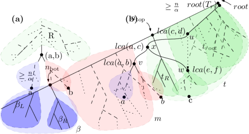
Figure 4: A left-heavy tree drawing displaying node $n_{\text{top}}$, node $n_{\text{bot}}$ and the relevant partitions

Lemma 3.3.

With probability of at least $\frac{\alpha-5}{2\alpha^{2}}$, a round of Algorithm 1 decreases the problem size of any recursive call by at least a factor of $\frac{\alpha-1}{\alpha}$, for a constant $\alpha>5$, thus experiencing a good split.

Proof 3.4.

Define the spine to be all nodes on the path from the root to its left-most leaf in a left-heavy drawing. Let $n_{\text{bot}}$ be the bottom-most node on the spine that has at least $n/\alpha$ of the nodes in its sub-tree. Conversely, let $n_{\text{top}}$ be the parent of the top-most spine node that has at most $(1-1/\alpha)\cdot n$ descendants. (See Figure 4.) Consider the three resulting trees obtained from separating at the incoming edge to $n_{\text{bot}}$ and the outgoing edge from $n_{\text{top}}$ to its left child. As shown in Figure 4, let $t$ be the resulting tree retaining the root, $\beta$ the tree rooted at $n_{\text{bot}}$ and $m$ the tree between $n_{\text{top}}$ and $n_{\text{bot}}$. Within $\beta$ let $\beta_{L}$ and $\beta_{R}$ be the trees rooted at the left and right child of $n_{\text{bot}}$. Similarly, for $t$, let $t_{R}$ be the tree rooted at the right child of $n_{\text{top}}$. Finally, let $t_{root}$ be the remaining tree when cut at $n_{\text{top}}$.

Consider the size of tree $\beta$, $|\beta|$, since this is the first tree rooted in the spine with over $n/\alpha$ nodes, then $\beta_{L}$ must have had strictly under $n/\alpha$ nodes. Since the trees are in left-heavy order, $\beta_{R}$ can have at most as many nodes as $\beta_{L}$ so $\frac{n}{\alpha}\leq|\beta|<\frac{2n}{\alpha}$. Furthermore, we know that $|\beta|+|m|+|t_{R}|+|t_{root}|+1=n$. Due to the left-heavy order, $|t_{R}|\leq|\beta|+|m|$. By definition of $n_{\text{top}}$, it’s necessary that $|t_{root}|<\frac{n}{\alpha}$, thus $2(|\beta|+|m|)+1>n-\frac{n}{\alpha}$ and $|\beta|+|m|>\left(\frac{\alpha-1}{2\alpha}\right)n-\frac{1}{2}$. Using the previous inequality and $|t|=n-|\beta|-|m|$, we find $|t|<\left(\frac{\alpha+1}{2\alpha}\right)n+\frac{1}{2}$. Also, $|m|=n-|t|-|\beta|$, so $|m|>n-\frac{5n+\alpha n}{2\alpha}$.

$$\frac{n}{\alpha}\leq|\beta|<\frac{2n}{\alpha},\qquad\frac{n}{\alpha}\leq|t|<\left(\frac{\alpha+1}{2\alpha}\right)n+\frac{1}{2},\qquad\left(\frac{\alpha-5}{2\alpha}\right)n<|m|\leq\left(\frac{\alpha-2}{\alpha}\right)n$$ (1)

Picking a leaf from $\beta$ and another from $m$ guarantees that $\beta\subseteq\left(A\cup\{a\}\right)$ and $t\subseteq R$. Thus, using Equation 1, each of the three sub-problem sizes, $|A\cup\{a\}|$, $|B\cup\{b\}|$, and $|R|$, will be at most $\left(\frac{\alpha-1}{\alpha}\right)n$, when $\alpha>5$. $Pr[\text{good split}]\geq Pr[\text{leaf in }\beta]\cdot Pr[\text{leaf in }m]$. Asymptotically, $Pr[\text{leaf in }\beta]\approx Pr[\text{node in }\beta]$, thus $Pr[\text{good split}]>\frac{\alpha-5}{2\alpha^{2}}$, which established the lemma.

Returning to the proof of Theorem 3.1, let $p=\frac{\alpha-5}{2\alpha^{2}}$. From Lemma 3.3, we expect it will take $1/p$ rounds to obtain a good split. Every good split will reduce the problem-size by at least a constant factor, $\frac{\alpha-1}{\alpha}$. Thus, we are guaranteed to have just a single node left after we get $N_{\textsc{splits}}=\log_{\frac{\alpha}{\alpha-1}}(n)$ good splits. Consider the geometric random variable, $X_{i}$, describing the number of rounds required to obtain the $i$-th good split, then $X=X_{1}+\ldots+X_{N_{\textsc{splits}}}$ describes the total number of rounds required by the algorithm. By linearity of expectation, $E[X]=\frac{2\alpha^{2}}{(\alpha-5)}\cdot N_{\textsc{splits}}=\frac{2\alpha^{2}}{(\alpha-5)}\cdot\log_{\frac{\alpha}{\alpha-1}}(n)$. Therefore, since $\alpha>5$ is a constant, this already implies an expected $O(\log n)$ rounds for Algorithm 1. Moreover, by a Chernoff bound for the sum of independent geometric random variables (see [22, 32]), $Pr\left[X>C\cdot E[X]\right]\leq e^{\frac{{-}(C-1)\cdot p\cdot N_{\textsc{splits}}}{5}}$ for any constant $C\geq 3$ and constant $\alpha>5$. Thus, the probability that we take over $C\cdot E[X]$ rounds is $O(1/n^{C-1})$. Therefore, by a union bound across the $n$ leaves, our algorithm completes in $O(\log n)$ rounds w.h.p.

Corollary 3.5.

Algorithm 1 is optimal when asking $\theta({n})$ queries per round.

The query complexity of Algorithm 1 matches an $\Omega(n\log n)$ lower bound for $Q(n)$, due to Kannan et al. [28]. Besides, we need $\Omega(\log{n})$ rounds if we have $\theta({n})$ processors; hence, the round complexity of Algorithm 1 is also optimal.

4 Reconstructing Phylogenetic Trees from Path Queries

Let $T=(V,E,r)$ be a rooted (biological or digital) phylogenetic tree with fixed degree, $d$. In this section, we show how a querier can reconstruct $T$ by issuing $Q(n)\in O(n\log n)$ path queries in $R(n)\in O(\log n)$ rounds, w.h.p., where $n=|V|$. We provide a lower bound to prove that our algorithm is optimal in terms of query complexity and round complexity. At the outset, the only thing we assume the querier knows is $n$ and $V$, that is, the vertex set for $T$, and that the names of the nodes in $V$ are unique, i.e., we may assume, w.l.o.g., that $V=\{1,2,\ldots,n\}$. The querier doesn’t know $E$ or $r$—learning these is his goal.

4.1 Algorithms

We start by learning $r$, which we show can be done via any maximum-finding algorithm in Valiant’s parallel model [43], which only counts parallel steps involving comparisons. The challenge, of course, is that the ancestor relationship in $T$ is, in general, not a total order, as required by a maximum-finding algorithm. This does not actually pose a problem, however.

Lemma 4.1.

Let $A$ be a parallel maximum-finding algorithm in Valiant’s model, with $O(f(n))$ span and $O(g(n))$ work. We can use $A$ to find the root, $r$ in a rooted tree $T=(V,E,r)$, using $R(n)\in O(f(n))$ rounds and $Q(n)\in O(g(n)+n)$ total queries.

Proof 4.2.

We pick an arbitrary vertex $v\in T$. In the first round, we perform queries $path(u,v)$ in parallel for every other vertex $u\in V$ to find $S$, the ancestor set for $v$. If $S=\emptyset$, then $v$ is the root. Otherwise, we know all the vertices in a path from root to the parent of $v$, albeit unsorted. Still, note that for $S$ the ancestor relation is a total order; hence, we can simulate $A$ with path queries to resolve the comparisons made by $A$. We have just a single round and $O(n)$ queries more than what it takes for $A$ to find the maximum. Thus, we can find the root in $O(f(n))$ rounds and $O(g(n)+n)$ queries.

Thus, by well-known maximum-finding algorithms, e.g., see [10, 40, 43]:

Corollary 4.3.

We can find $r$ of a rooted tree $T=(V,E,r)$ deterministically in $O(\log\log n)$ rounds and $O(n)$ queries.

Determining the rest of the structure of $T$ is more challenging, however. At a high level, our approach to solving this challenge is to use a separator-based divide-and-conquer strategy, that is, find a “near” edge-separator in $T$, divide $T$ using this edge, and recurse on the two remaining subtrees in parallel. The difficulty, of course, is that the querier has no knowledge of the edges of $T$; hence, the very first step, finding a “near” edge-separator, is a bottleneck computation. Fortunately, as we show in Lemma 4.4, if $v$ is a randomly-chosen vertex, then, with probability depending on $d$, the path from root $r$ to $v$ includes an edge-separator.

Lemma 4.4.

Let $T=(V,E,r)$ be a rooted tree of degree $d$ and let $v$ be a vertex chosen uniformly at random from $V$. Then, with probability at least $\frac{1}{d}$, an even-edge-separator is one of the edges on the path from $r$ to $v$.

Proof 4.5.

By Lemma 2.5, $T$ has an even-edge-separator. Let $e=(x,y)$ be an even-edge-separator for $T=(V,E,r)$ and let ${T^{\prime}=(V^{\prime},E^{\prime},y)}$ be the subtree rooted at $y$ when we remove $e$. Then, every path from $r$ to each $v\in V^{\prime}$ must contain $e$. By Definition 2.4, $T^{\prime}$ has at least $|V|/d$ vertices. Therefore, if we choose $v$ uniformly at random from $V$, then with probability $\frac{|V^{\prime}|}{|V|}\geq\frac{1}{d}$, the path from $r$ to $v$ contains $e$.

Definition 4.6.

(splitting-edge) In a degree-$d$ rooted tree, an edge $(parent(s),s)$ is a splitting-edge if $\frac{|V|}{d+2}\leq\textit{}{D}(s)\leq\frac{|V|(d+1)}{d+2}$, where $\textit{D}(s)$ is the number of descendants of $s$.

Note that a degree-$d$ rooted tree $T$ always has a splitting-edge, as every even-edge-separator is also a splitting-edge and by Lemma 2.5, it always has an even-edge-separator—a fact we use in our tree-reconstruction algorithm, which we describe next. This recursive algorithm (given in pseudo-code in Algorithm 3), assumes the existence of a randomized method, find-splitting-edge, which returns a splitting-edge in $T$, with probability $\Omega(1/d)$, and otherwise returns $\mathit{Null}$. Our reconstruction algorithm is therefore a randomized recursive algorithm that takes as input a set of vertices, $V$, with a (known) root vertex $r\in V$, and returns the edge set, $E$, for $V$. At a high level, our algorithm is to repeatedly call the method, find-splitting-edge, until it returns a splitting-edge, at which point we divide the set of vertices using this edge and recurse on the two resulting subtrees.

1

2 Function reconstruct-rooted-tree($V,r$):

3       $E\leftarrow\emptyset$

4      if $|V|\leq g$ then // $g$ is a chosen constant

5            return edges found by a quadratic brute-force algorithm

6            while true do

7                 Pick a vertex $v\in V$ uniformly at random

8                 for $z\in V$ do in parallel

9                     Perform query $path(z,v)$

10                      Let $Y$ be the vertex set of the path from $r$ to $v$

11                      splitting-edge $\leftarrow$ find-splitting-edge$(v,Y,V)$

12                      if splitting-edge $\neq$ $\mathit{Null}$ then

13                           $(u,w)\leftarrow$ splitting-edge

14                           $E\leftarrow E\cup\{(u,w)\}$

15                           for $z\in V$ do in parallel

16                               Perform query $path(w,z)$

17                                split $V$ into $V_{1},V_{2}$ at $(u,w)$ using query results

18                                parallel do

19                                     $E\leftarrow E\cup\textsf{reconstruct-rooted-tree}(V_{1},w)$

20                                    $E\leftarrow E\cup\textsf{reconstruct-rooted-tree}(V_{2},r)$

21                                    

22                                    return $E$

23                                    

24                                    

Algorithm 3 Reconstruct a rooted tree with path queries

In more detail, during each iteration of a repeating while loop, we choose a vertex $v\in V$ uniformly at random. Then, we find the vertices on the path from $r$ to $v$ and store them in a set, $Y$, using the fact that a vertex, $z$, is on the path from $r$ to $v$ if and only if $path(z,v)=1$. Then, we attempt to find a splitting-edge using the function find-splitting-edge (shown in pseudo-code in Algorithm 4). If find-splitting-edge is unsuccessful, we give up on vertex $v$, and restart the while loop with a new choice for $v$. Otherwise, find-splitting-edge succeeded and we cut the tree at the returned splitting-edge, $(u,w)$. All vertices, $z\in V$, where $path(w,z)=1$ belong to the subtree rooted at $w$, thus belonging to $V_{1}$, whereas the remaining vertices belong to $V_{2}$ and the partition containing both $u$ and rooted at $r$. Thus, after cutting the tree we recursively reconstruct-rooted-tree on $V_{1}$ and $V_{2}$.

1

2 Function find-splitting-edge($v,Y,V$):

3      

4      splitting-edge $\leftarrow$ $\mathit{Null}$

5       $m=C_{1}\sqrt{|V|}$, $K=C_{2}\log{|V|}$

       Phase 1: 

6            if $|Y|>|V|/K$ then

7                 $S\leftarrow$ subset of $m$ random elements from $Y$

8                $S\leftarrow S\cup{\{v,r\}}$

9                for each $s\in S$ do in parallel

10                      $X_{s}\leftarrow$ subset of $K$ random elements from $V$

11                     Perform queries to find $count(s,X_{s})$

12                     

13                     if $\forall s\in S:count(s,X_{s})<\frac{K}{d+1}$  then return $\mathit{Null}$

14                     

15                     if $\forall s\in S:count(s,X_{s})>\frac{Kd}{d+1}$ then return $\mathit{Null}$

16                     

17                     if $\exists s\in S:\frac{K}{d+1}\leq count(s,X_{s})\leq\frac{Kd}{d+1}$ then

                           return verify-splitting-edge$(s,V)$

18                          

19                          for each $\{a,b\}\in S$ do in parallel

20                                perform query $path(a,b)$

21                                Find $w,z$ such that they are two consecutive nodes in the sorted order of $S$ such that $count(w,X_{w})>\frac{Kd}{d+1}$ and $count(z,X_{z})<\frac{K}{d+1}$

22                                $Y\leftarrow$ nodes from $Y$ in the path from $w$ to $z$

23                               

                                Phase 2: 

24                                     if $|Y|>|V|/K$ then return $\mathit{Null}$

25                                     for each $s\in Y$ do in parallel

26                                          $X_{s}\leftarrow$ subset of $K$ random elements from $V$

27                                         Perform queries to find $count(s,X_{s})$

28                                          if $\exists s\in Y$ s.t. $\frac{K}{d+1}\leq count(s,X_{s})\leq\frac{Kd}{d+1}$ then

                                               return verify-splitting-edge$(s,V)$

29                                              

30                                              

31                                               return $\mathit{Null}$

Algorithm 4 Finding a splitting-edge from vertex set, $Y$, on the path from vertex $v$ to the root $r$

The main idea for our efficient tree reconstruction algorithm lies in our find-splitting-edge method (see Algorithm 4), which we describe next. This method takes as input the vertex $v$, the vertex set $Y$, (comprising the vertices on the path from $r$ to $v$), and the vertex set $V$. As we show, with probability depending on $d$, the output of this method is a splitting-edge; otherwise, the output is $\mathit{Null}$. Our algorithm performs a type of “noisy” search in $Y$ to either locate a likely splitting-edge or return $\mathit{Null}$ as an indication of failure.

Our find-splitting-edge algorithm consists of two phases. We enter Phase 1 if the size of path $Y$ is too big, i.e., $|Y|>|V|/K=\frac{|Y|}{C_{2}\log{|V|}}$, where $C_{2}$ is a predetermined constant and $K=C_{2}\log|V|$. The purpose of this phase is either to pass a shorter path including an even-edge-separator to the second phase or to find a splitting-edge in this iteration. The search on the set $Y$ is noisy, because it involves random sampling. In particular, we take a random sample $S$ of size $m=C_{1}\sqrt{|V|}$ from path $Y$ (where $C_{1}$ is a predetermined constant). We include $r$ and $v$, the two endpoints of the path $Y$, to $S$. Then, we estimate the number of descendants of $s$, $\textit{D}(s)$, for each $s\in S$. To estimate this number for each $s\in S$, we take a random sample $X_{s}$ of $K$ elements from $V$ and we perform queries to find $count(s,X_{s})$. Here, we use $m\cdot K\in O(\sqrt{|V|}\log{|V|})$ queries in a single round. Then, if all the estimates were less than $K/(d+1)$, we return $\mathit{Null}$ as an indication of failure (we guess that all the nodes on the path $Y$ have too few descendants to be a separator). Similarly, if all the estimates were greater than $\frac{Kd}{d+1}$, we return $\mathit{Null}$ (we guess that all the nodes on the path $Y$ have too many descendants to be a separator). If there exists a node $s$ such that $\frac{K}{d+1}\leq count(s,X_{s})\leq\frac{Kd}{d+1}$, we check if $s$ is a splitting-edge by counting its descendants using a function, verify-splitting-edge. This function takes vertex $s$ and the full vertex set $V$ to return edge $($find-parent$(s,V),s)$ if $\frac{|V|}{d+2}\leq count(s,V)\leq|V|\cdot\frac{d+1}{d+2}$ and return $\mathit{Null}$ otherwise.

If neither of these three cases happens, we perform queries to sort elements of $S$ using a trivial quadratic work parallel sort which takes $O(m^{2})\in O(|V|)$ queries in a single round. We know that two consecutive nodes $w$ and $z$ exist on the sorted order of $S$, where $count(w,X_{w})>\frac{Kd}{d+1}$ and $count(z,X_{z})<\frac{K}{d+1}$. We find all the nodes on $Y$ starting at $w$ and ending at $z$, and use this as our new path $Y$.

In Phase 2, we expect a path of size under $|Y|/K$, we will later prove this is true with high probability. Otherwise, we just return $\mathit{Null}$. In this phase, we estimate the number of descendants much like we did in the previous phase, except the only difference is that we estimate the number of descendants for all the nodes on our new path $Y$. If there exists a node $s\in Y$ such that $\frac{K}{d+1}\leq count(s,X_{s})\leq\frac{Kd}{d+1}$, we verify if it is a splitting-edge, as described earlier.

Finally, let us describe how we find the parent of a node $s$ in $V$. We first find, $Y$, the set of ancestors of $v$ in $V$ in parallel using $|V|$ queries. Let $x\succ y$ describe the total order of nodes in path $Y$, where for any $x,y\in Y:x\succ y$ if and only if $path(x,y)=1$. The parent of $s$ is the lowest vertex on the path. Then, the key idea is that if $|Y|\in O(\sqrt{|V|})$, we can sort them using $O(|V|)$ queries. If the path is greater than this amount, we instead use $S$, a sample of size $O(\sqrt{|V|})$ from the path. Next, we sort the sample to obtain $x_{1}<\ldots<x_{m}$ for $S$ and then find all of the nodes in $Y$ which are less than the smallest sample $x_{1}$. Finally, we replace $Y$ with these descendants of $x_{1}$ and repeat the whole procedure again. We later prove that with high probability after two iterations of this sampling, the size of the path is $O(\sqrt{|V|})$, allowing us to sort all nodes in $Y$ to return the minimum (see Function 4.1).

[t]    find-parent($s,V$) find $Y$, ancestor set of $s$ from $V$ using $|V|$ queries in parallel $m=C_{1}\sqrt{|V|}$ for $i\leftarrow 1$ to $2$ $\And|Y|>m$ do

2      $S\leftarrow$ random subset of $Y$ with $m$ elements sort $S$ as $x_{1}<...<x_{m}$ using $O(m^{2})$ queries in parallel find $Y^{\prime}=\{u\in Y\mid u\leq x_{1}\}$ using $O(|Y|)$ queries in parallel, replace $Y$ with $Y^{\prime}$

3      if $|Y|\leq m$ then

4           sort $Y$ using $O(m^{2})$ queries in parallel return (minimum of this path)

return $\mathit{Null}$  

4.2 Analysis

The correctness of the algorithm follows from the fact that our method first finds the root, $r$, of $T$ and then finds the parent of each other node, $v$ in $T$.

Theorem 4.7.

Given a set, $V$, of nodes of a rooted tree, $T$, such as a biological or digital phylogenetic tree, with degree bounded by a fixed constant, $d$, we can construct $T$ using path queries with round complexity, $R(n)$, that is $O(\log n)$ and query complexity, $Q(n)$, that is $O(n\log n)$, with high probability.

Our proof of Theorem 4.7 begins with Lemma 4.8.

Lemma 4.8.

In a rooted tree, $T=(V,E,r)$, let $Y$ be a (directed) path, where $|Y|>m=C_{1}\sqrt{|V|}$. If we take a sample, $S$, of $m$ elements from $Y$, then with probability $1-\frac{1}{|V|}$, every two consecutive nodes of $S$ in the sorted order of $S$ are within distance $O\left(\frac{|Y|\log{|V|}}{\sqrt{|V|}}\right)$ from each other in $Y$.

Proof 4.9.

Note that some nodes of $Y$ may be picked more than once as we pick $S$ in parallel. Divide the path $Y$ into $\frac{\sqrt{|V|}}{\log|V|}$ equal size sections (the difference between the size of any two sections is at most 1). For each $1\leq i\leq{\frac{\sqrt{|V|}}{\log|V|}}$, let $A_{i}$ be the subset of $S$ lying in the $i\textsuperscript{th}$ section of $Y$. (See Figure 5.) It is clear that each node $s\in S$ ends up in section $i$ with probability $\frac{\log{|V|}}{\sqrt{|V|}}$, and therefore, for each $1\leq i\leq{\frac{\sqrt{|V|}}{\log|V|}}$, ${E}\left[|A_{i}|\right]=C_{1}\log{|V|}$. Thus, using standard a Chernoff bound, $\Pr\left[|A_{i}|=0\right]<\frac{1}{|V|^{2}}$ for any constant $C_{1}>6\ln{10}$. Using a union bound, all the sections are non-empty with probability at least $1-\frac{1}{|V|}$. Hence, the distance between any two consecutive nodes of $S$ from each other in $Y$ is at most $\frac{2|Y|\log{|V|}}{\sqrt{|V|}}$.

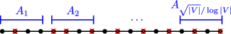
Figure 5: Illustration of how scattered sample $S$ is on path $Y$. The $i\textsuperscript{th}$ blue interval represents the $i\textsuperscript{th}$ section of $Y$, the black dots correspond to the nodes on the path $Y$, and red crossed marks represent elements of $S$.

Lemma 4.8 allows us to analyze the find-parent method, as follows.

Lemma 4.10.

The find-parent$(s,V)$ method outputs the parent of $s$ with probability at least $1-2/|V|$, with $Q(n)\in O(n)$ and $R(n)\in O(1)$.

Proof 4.11.

The find-parent method succeeds if, after the for loop, the size of the set of remaining ancestors of $s$, $Y$, is $|Y|\leq m$, so it is enough to show that this occurs with probability at least $1-2/|V|$. By Lemma 4.8, the size of $Y$ at the end of the first iteration is $|Y|\in O(m\log|V|)$, with probability at least $1-1/|V|$. Similarly, a second iteration, if required, further reduces the size of $Y$ into $|Y|\in o(m)$, with probability at least $1-1/|V|$. Thus, by a union bound, the probability of success is at least $1-2/|V|$.

The query complexity can be broken down as follows, where $m\in O(\sqrt{|V|})$:

1. $O(|V|)$ queries in 1 round to determine the ancestor set, $Y$, of $s$.

2. $O(m^{2})+O(|Y|)\in O(|V|)$ queries in 2 rounds for each of the (at most) 2 iterations performed in find-parent, whose purpose is to discard non-parent ancestors of $s$ in $Y$.

3. $O(m^{2})\in O(|V|)$ to find, in 1 round, the minimum among the remaining ancestors of $Y$ (at most $m$ w.h.p.). If $|Y|>m$, then no further queries are issued.

In total, the above amounts to $Q(n)\in O(n)$ and $R(n)\in O(1)$.

We next analyze the find-splitting-edge method.

Lemma 4.12.

Any call to find-splitting-edge returns true with probability $\frac{1}{2d}$; hence Algorithm 3 calls find-splitting-edge $O(d)$ times in expectation.

Proof 4.13.

By Lemma 4.4, we know that if we pick a vertex $v$, uniformly at random, then with probability $\frac{1}{d}$, an even-edge-separator lies on the path from $r$ to $v$. We show that if there is such an even-edge-separator (Definition 2.4) on that path, find-splitting-edge($v,Y,V$) returns a splitting-edge (Definition 4.6) with probability at least $\frac{1}{2}$, and otherwise returns $\mathit{Null}$. Using an intricate Chernoff-bound analysis (see Appendix A), we can prove that there exists a constant $C_{2}>0$, as used in line 4 of Algorithm 4 such that the following probability bounds always hold:

$$\begin{cases}\Pr\left(count(s,X_{s})\geq\frac{K}{d+1}\right)\geq 1-\frac{1}{|V|^{2}}&\mbox{if }count(s,V)\geq\frac{|V|}{d},\\ \Pr\left(count(s,X_{s})\leq K\frac{d}{d+1}\right)\geq 1-\frac{1}{|V|^{2}}&\mbox{if }count(s,V)\leq|V|\frac{d-1}{d},\\ \end{cases}$$ (2)

$$\begin{cases}\Pr\left(count(s,X_{s})<\frac{K}{d+1}\right)\geq 1-\frac{1}{|V|^{2}}&\mbox{if }count(s,V)<\frac{|V|}{d+2},\\ \Pr\left(count(s,X_{s})>K\frac{d}{d+1}\right)\geq 1-\frac{1}{|V|^{2}}&\mbox{if }count(s,V)>|V|\frac{d+1}{d+2}\\ \end{cases}$$ (3)

It is clear that we either return a splitting-edge or $\mathit{Null}$ when passing through verify-splitting-edge. We break the probability of returning $\mathit{Null}$ according to the phases. We call a vertex $v$ ineligible if $count(v,V)<\frac{|V|}{d+2}$ or $count(v,V)>\frac{|V|(d+1)}{d+2}$ ($(parent(v),v)$ is not a splitting-edge). On the other hand, we call vertex $v$ candidate if after estimating the number of its descendants: $\frac{K}{d+1}\leq count(v,X)\leq\frac{Kd}{d+1}$. Let $(a,b)$ be an even-edge-separator on path $Y$.

Phase 1:

• lines 4,4: By Definition 2.4, $\frac{|V|}{d}\leq count(b,V)\leq\frac{|V|(d-1)}{d}$. We add $\{r,v\}$ to $S$ in line 4 of the algorithm (the two endpoints of path $Y$). Notice that $\frac{|V|}{d}\leq count(b,V)\leq count(r,V)$ and that $count(v,V)\leq count(b,V)\leq\frac{|V|(d-1)}{d}$. So, by Equation 2, with probability at least $1-\frac{2}{|V|^{2}}$, $count(r,X_{r})\geq\frac{K}{d+1}$ and $count(v,X_{v})\leq\frac{Kd}{d+1}$, and consequently, we don’t return $\mathit{Null}$ in lines 4,4 of the algorithm.

• line 4: Equation 3 shows that an ineligible node is not a candidate with probability $1-\frac{1}{|V|^{2}}$. Thus, by a union bound, none of our candidates is ineligible in line 4 with probability at least $1-\frac{|S|}{|V|^{2}}$. Moreover, if there exists a candidate $s$ in $S$, the algorithm outputs a splitting-edge $(parent(s),s)$ with probability at least $1-\frac{2}{|V|}$, by Lemma 4.10.

• lines 4,4: Let us partition $S$ into $S_{l}$ and $S_{r}$ (see Figure 6), as follows:

  $$S_{l}=\{s\in S\mid count(s,V)>count(b,V)\},\qquad S_{r}=\{s\in S\mid count(s,V)<count(b,V)\}$$

  Then, by definition of $b$:

  $$\forall s\in S_{l}: count(s,V)>|V|/d,\qquad \forall s\in S_{r}: count(s,V)<|V|(d-1)/d.$$

  and thus, by Equation 2 and a union bound, we have with probability at least $1-\frac{|S|}{|V|^{2}}$:

  $$\forall s\in S_{l}: count(s,X_{s})\geq K/(d+1),\qquad \forall s\in S_{r}: count(s,X_{s})\leq Kd/(d+1).$$

  Finally, since $S$ does not contain any candidate nodes (otherwise we would have picked them in line 4), the above inequalities imply that:

  $$\forall s\in S_{l}: count(s,X_{s})>Kd/(d+1),\qquad \forall s\in S_{r}: count(s,X_{s})<K/(d+1).$$

  Therefore, $w\in S_{l}$ and $z\in S_{r}$, which implies that the subpath from $w$ to $z$ in $Y$ must include vertex $b$. This means that with probability $1-O(\frac{1}{|V|})$, we either find a splitting-edge in this phase or pass $b$ to the next phase.

Now, consider Phase 2:

• line 4: Here, if $|Y|>|V|/K$, then we have passed through Phase 1. Using Lemma 4.8, we know that since $S$ was a sample of size $C_{1}\sqrt{|V|}$ from $Y$, with probability $1-\frac{1}{|V|}$ the distance between any two consecutive nodes of $S$ in $Y$ was $O(|Y|\frac{\log{|V|}}{\sqrt{|V|}})\in O(\sqrt{|V|}\log{|V|})$. Thus, the size of path $Y$ after passing through line 4 is at most $O(\sqrt{|V|}\log{|V|})$. Thus, the probability of returning $\mathit{Null}$ in line 4 is at most $\frac{2}{|V|}$.

• line 4: By Equation 3, with probability at least $1-\frac{|Y|}{|V|^{2}}$, no ineligible node is between candidate set. Besides, for a candidate node $s$, the algorithm outputs a splitting-edge $(parent(s),s)$ with probability at least $1-\frac{2}{|V|}$, by Lemma 4.10.

• line 4: The probability that we return $\mathit{Null}$ here is equal to the probability that our candidate set in line 4 is empty. By Equation 2, with probability at least $1-\frac{2}{|V|^{2}}$, $b$ is between candidates at line 4 and candidate set is non-empty. Thus, the total probability of failing to return a splitting-edge in this phase is at most $O(\frac{1}{|V|})$.

Therefore, for $|V|$ greater than the chosen constant $g$, the probability of returning $\mathit{Null}$ in the existence of an even-edge-separator is at most $O(\frac{1}{|V|})\leq 1/2$. Thus, the probability of returning a splitting-edge in any call to find-splitting-edge is at least $\frac{1}{2d}$.

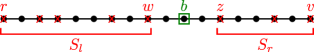
Figure 6: Illustration of the path reduction in Phase 1 of find-splitting-edge. At the end of this phase, the path $Y$ is trimmed down into the subpath consisting of the nodes between $w$ and $z$, which contains $b$ w.h.p.

Lemma 4.14.

The subroutine find-splitting-edge$(v,Y,V)$ has query complexity, $Q(n)$, that is $O(|V|)$, and round complexity, $R(n)$, that is $O(1)$.

Proof 4.15.

The queries done by find-splitting-edge$(v,Y,V)$, in the worst case, can be broken down as follows, where $m=O(\sqrt{|V|})$:

Phase 1: A total of $O(|V|)$ queries in $O(1)$ rounds, consisting of:

• $O(mK)\in O(\sqrt{|V|}\log|V|)$ queries in one round for estimating the number of descendants for the $m$ samples.

• $O(m^{2})\in O(|V|)$ queries in one round for sorting the $m$ samples.

• $O(|Y|)\in O(|V|)$ queries in a round to find the subpath of $Y$ that is the input for Phase 2.

• $O(|V|)$ queries in $O(1)$ rounds for determining the parent of $s$ (see Lemma 4.10).

Phase 2: If we enter this phase, it spends $O(|V|)$ queries in $O(1)$ rounds:

• $|Y|\cdot K\in O(|V|)$ queries in one round to evaluate count($s,X_{s}$) for each $s\in Y$.

• $O(|V|)$ queries in one round to find the number of descendants of node $s$.

• $O(|V|)$ queries in $O(1)$ rounds to determine the parent of $s$ (see Lemma 4.10).

Overall, the above break down amounts to $Q(n)\in O(n)$ and $R(n)\in O(1)$.

Now, recall Theorem 4.7: Given a set, $V$, of nodes of a rooted tree, $T$, such as a biological or digital phylogenetic tree, with degree bounded by a fixed constant, $d$, we can construct $T$ using path queries with round complexity, $R(n)$, that is $O(\log n)$ and query complexity, $Q(n)$, that is $O(n\log n)$, with high probability.

Proof 4.16.

The expected query complexity $Q(n)$ of Algorithm 3 is dominated by the two recursive calls $\left(Q\left(\frac{n}{d+2}\right)\text{ and }Q\left(\frac{n(d+1)}{d+2}\right)\right)$ and the calls to find-splitting-edge. By Lemma 4.12, we call find-splitting-edge an expected $O(d)$ times, incurring a cost of $O\left(dn\right)\in O(n)$ path queries in $O(d)\in O(1)$ rounds (see Lemma 4.14). Thus, $Q(n)$ and $R(n)$ are:

$$Q(n)=Q\left(\frac{n}{d+2}\right)+Q\left(\frac{n(d+1)}{d+2}\right)+O\left(n\right),$$

$$R(n)=\max\left(R\left(\frac{n}{d+2}\right),R\left(\frac{n(d+1)}{d+2}\right)\right)+O(1)$$

which shows it needs $Q(n)\in O(n\log n)$ and $R(n)\in O(\log n)$ in expectation. To prove the high probability results, note that the main algorithm is a divide-and-conquer algorithm with two recursive calls per call; hence, it can be modeled with a recursion tree that is a binary tree, $B$, with height $h=O(\log_{\frac{d+2}{d+1}}n)=O(\log n)$. For any root-to-leaf path in $B$, the time taken can modeled as a sum of independent random variables, $X=X_{1}+X_{2}+\cdots+X_{h}$, where each $X_{i}$ is the number of calls to find-splitting-edge (each of which uses $O(|V|)$ queries in $O(1)$ rounds) required before it returns true, which is a geometric random variable with parameter $p=\frac{1}{2d}$. Thus, by a Chernoff bound for sums of independent geometric random variables (e.g., see [22, 32]), the probability that $X$ is more than $O(d\log_{\frac{d+2}{d+1}}n)$ is at most $1/n^{c+1}$, for any given constant $c\geq 1$. The theorem follows, then, by a union bound for the $n$ root-to-leaf paths in $B$.

4.3 Lower Bound

We establish the following simple lower bound, which extends and corrects lower-bound proofs of Wang and Honorio [45].

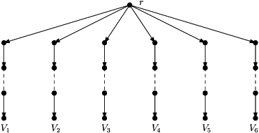
Figure 7: Illustration of the $\Omega(dn+n\log n)$ lower bound for path queries in directed rooted trees (shown for $d=6$).

Theorem 4.17.

Reconstructing an $n$-node, degree-$d$ tree requires $\Omega(dn+n\log n)$ path queries. This lower bound holds for the worst case of a deterministic algorithm and for the expected value of a randomized algorithm.

Proof 4.18.

Consider an $n$-node, degree-$d$ tree, $T$, as shown in Figure 7, which consists of a root, $r$, with $d$ children, each of which is the root of a chain, $T_{i}$, of at least one node rooted at a child of $r$. Since a querier, Bob, can determine the root, $r$, in $O(n)$ queries anyway, let us assume for the sake of a lower bound that $r$ is known; hence, no additional information is gained by path queries involving the root. Let us denote the vertices in chain $T_{i}$ as $V_{i}$. In order to reconstruct $T$, Bob must determine the nodes in each $V_{i}$ and must also determine their order in $T_{i}$. For a given path query, $path(u,v)$, say this query is internal if $u,v\in V_{i}$, for some $i\in[1,d]$, and this query is external otherwise. Note that even if Bob knows the full structure of $T$ except for a given node, $v$, he must perform at least $d-1$ external queries in the worst case, for a deterministic algorithm, or $\Omega(d)$ external queries in expectation, for a randomized algorithm, in order to determine the chain, $T_{i}$, to which $v$ belongs. Furthermore, the result of an (internal or external) query, $path(u,v)$, provides no additional information for a vertex $w$ distinct from $u$ and $v$ regarding the set, $V_{i}$, to which $w$ belongs. Thus, Bob must perform $\Omega(d)$ external queries for each vertex $v\not=r$, i.e., he must perform $\Omega(dn)$ external queries in total. Moreover, note that the results of external queries involving a vertex, $v$, provide no information regarding the location of $v$ in its chain, $T_{i}$. Even if Bob knows all the vertices that comprise each $V_{i}$, he must determine the ordering of these vertices in the chain, $T_{i}$, in order to reconstruct $T$. That is, Bob must sort the vertices in $V_{i}$ using a comparison-based algorithm, where each comparison is an internal query involving two vertices, $u,v\in V_{i}$. By well-known sorting lower bounds (which also hold in expectation for randomized algorithms), e.g., see [22, 11], determining the order of the vertices in each $T_{i}$ requires $\Omega(|V_{i}|\log|V_{i}|)$, as one of the chain can be as great as $n-d$ vertices, then he needs $\Omega(n\log n)$ internal queries.

Corollary 4.19.

Algorithm 3 is optimal for bounded-degree trees when asking $\theta({n})$ queries per round.

The query complexity of Algorithm 3 matches the lower bound provided by Theorem 4.17 when $d$ is constant. Besides, we need $\Omega(d+\log{n})$ rounds if we have $\theta({n})$ processors; hence, the round complexity of Algorithm 3 is also optimal.

5 Experiments

Given that both of our algorithms are randomized and perform optimally with high probability, we carried out experiments to analyze the practicality of our algorithms and compare their performance with the best known algorithms for reconstructing rooted trees.

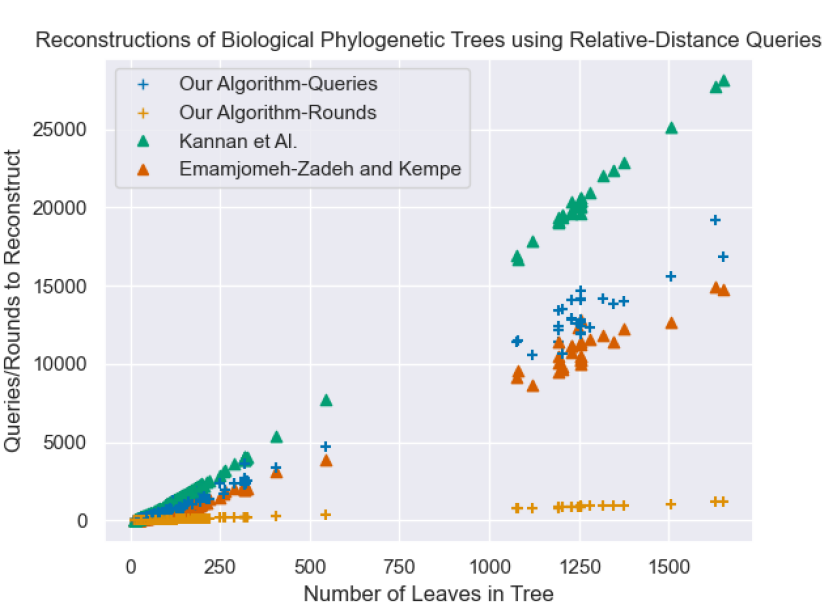
Figure 8: A scatter plot showing the number of queries and rounds for each of the three tree reconstruction algorithms for real trees from TreeBase. Since our algorithm is parallel, we include round complexity to serve as a comparison for the sequential complexity.

5.1 Reconstructing Biological Phylogenetic Trees

In order to assess the practical performance of Algorithm 1, we performed experiments using synthetic phylogenetic trees and real-world biological phylogenetic trees from the phylogenetic library TreeBase [35], which is a database of biological phylogenetic trees, comprising over 100,000 distinct taxa in total.

We implemented an oracle interface, instantiated it with the relevant trees, and implemented our algorithm along with two other phylogenetic tree reconstruction algorithms that use relative-distance queries. The first is by Emamjomeh-Zadeh and Kempe [17], which is a randomized sequential divide-and-conquer algorithm. The second is by Kannan et al. [28], where they use a sequential deterministic procedure reminiscent of insertion-sort. All three algorithms achieve the optimal asymptotic query complexity of $\Theta(n\log n)$ in expectation.

Real Data.

We instantiated our oracles with 1,220 biological phylogenetic trees from the TreeBase collection and used them to run all three algorithms. The results, shown in Figure 8, suggest that our algorithm outperforms the algorithm by Kannan et al., both in terms of its round complexity and query complexity. However our algorithm almost matches Emamjomeh-Zadeh and Kempe’s in terms of total queries and we believe the small difference is a direct result of the cost incurred while parallelizing the link step of Algorithm 1. It remains clear that Algorithm 1 outperforms the two other algorithms when considering the parallel speed-up.

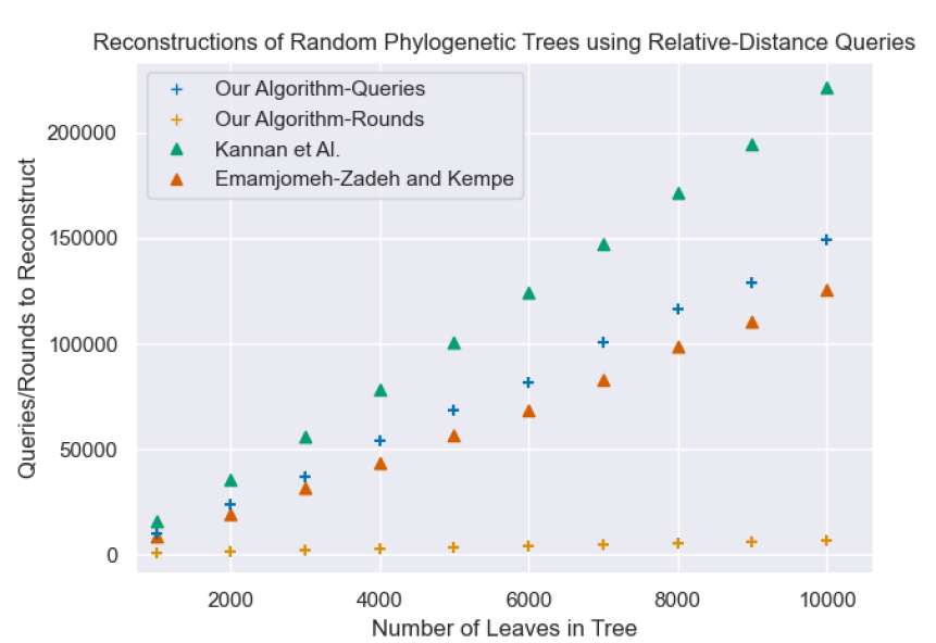
Figure 9: A plot showing the average number of queries and rounds for each of the three tree reconstruction algorithms. Each data point represents the average for 10 randomly generated trees.

Synthetic Data.

We also tested this algorithm using synthetic data and found similar results, detailed in Figure 9. We detail the method used to generate these random tree instances in Section 5.2, however, given our algorithm’s strict focus on biological phylogenetic trees, we use only full binary trees, where each internal node has exactly two children.

5.2 Reconstructing Phylogenetic Trees from Path Queries

To assess the practical performance of our method for reconstructing (biological and digital) phylogenetic trees from path queries, we performed experiments using both synthetic and real data to compare our algorithm with the algorithm by Wang and Honorio [45], which is the best known reconstruction algorithm for phylogenetic trees from path queries. Our experimental results provide evidence that Algorithm 3 provides significant parallel speedup, while simultaneously improving the total number of queries.

Synthetic Data.

In order to generate random instances of trees with maximum degree, $d$, we synthesized a data set of random degree-$d$ trees of $n$ nodes for different values of $n$ and $d$. To generate a random tree, $T$, for a given $n$ and $d$, we first generated a random Prüfer sequence [36] of a labeled tree, which defines a unique sequence associated with that tree, and converted it to its associated tree. In particular, each $n$-node tree $T=(V,E)$ has a unique code sequence $s_{1},s_{2},\dots,s_{n-2}$, where $s_{i}\in V$ for all $1\leq i\leq n-2$ and every node $v_{i}\in V$ of degree $d_{i}$ appears exactly $d_{i}-1$ times in this sequence. Therefore, in order to generate random degree-$d$ rooted trees we generate a random Prüfer sequence while imposing conditions that: (i) all vertices appear at most $d-1$ times in the code and (ii) there is at least one node such that it appears exactly $d-1$ times. Converting each such sequence to its associated tree gave us a random degree-$d$ tree instance that we used in our experiments.

Since our parallel reconstruction algorithm using path queries is parameterized by a constant, $C_{2}$, we ran our algorithm using different values for $C_{2}$. The constant $C_{2}$ controls sample size from $V$ used to estimate the number of descendants of a node. Furthermore, to reduce noise from randomization, each data-point will be averaged for 3 runs on 10 randomly generated trees. In Figure 10, we compare our algorithm’s rounds and total number of queries with the one by Wang and Honorio [45], for fixed degree trees $d=5$ and varying tree-sizes. These results provide empirical evidence that our algorithm provides a noticeable speedup in parallel round complexity while also outperforming the algorithm by Wang and Honorio [45] in total number of queries.

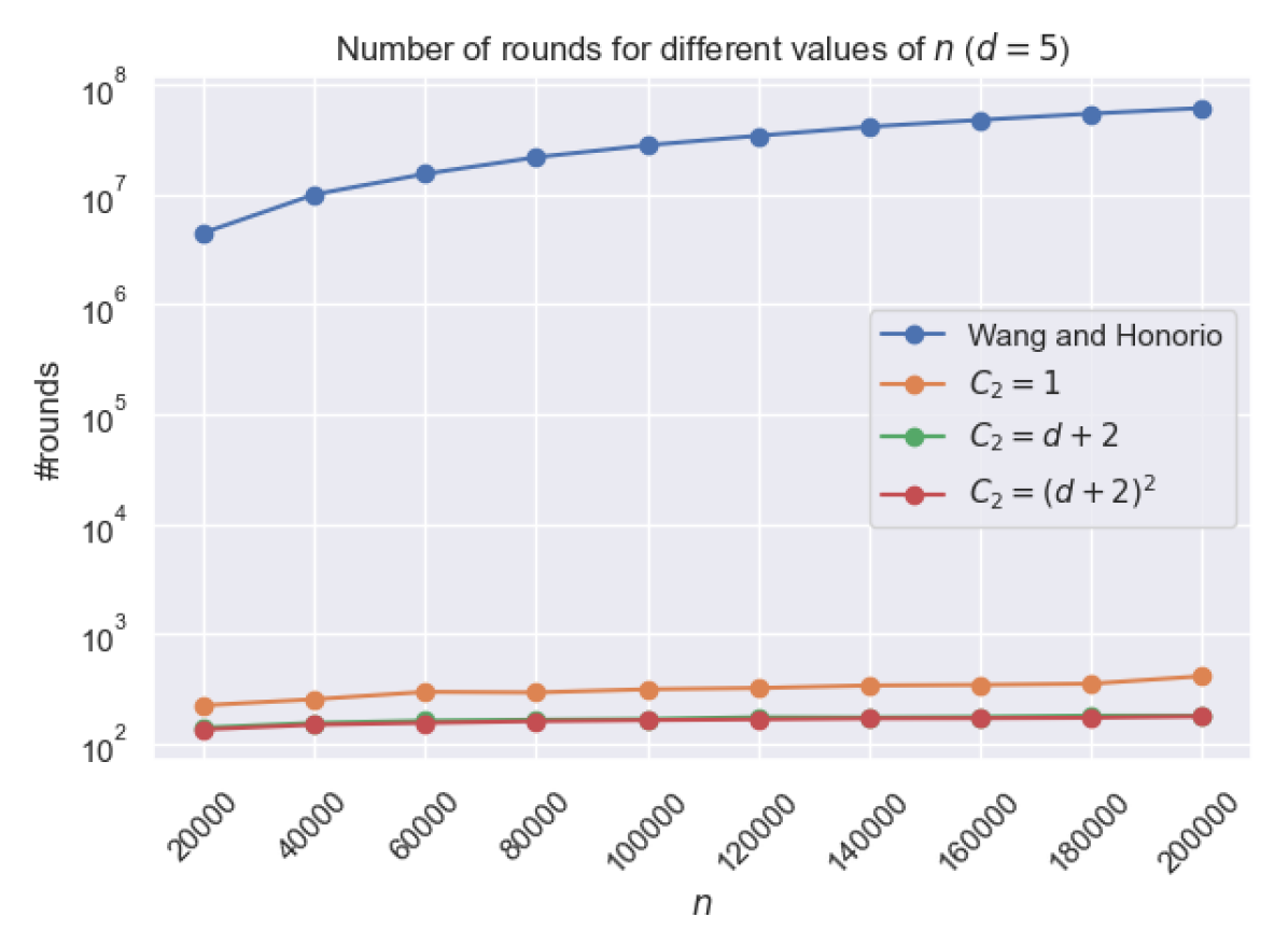
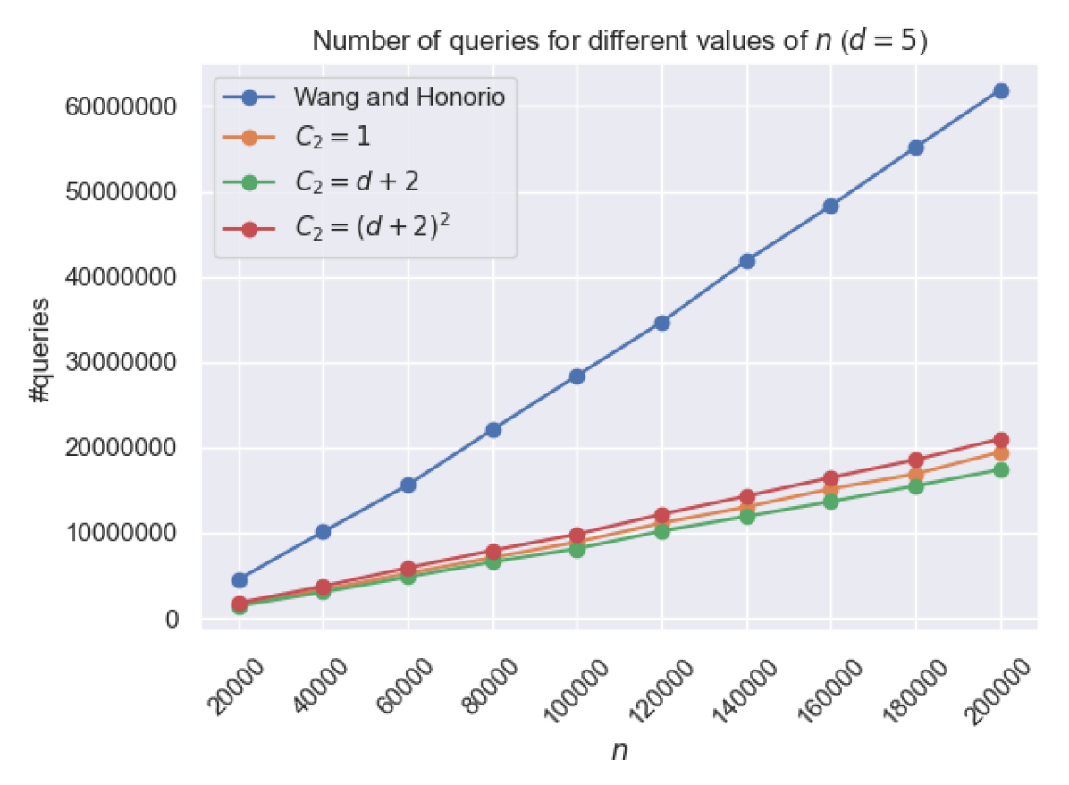
Figure 10: Comparing Our Algorithm’s number of rounds (left) and total queries (right) with Wang and Honorio’s [45], for fixed $d=5$ and varying $n$.

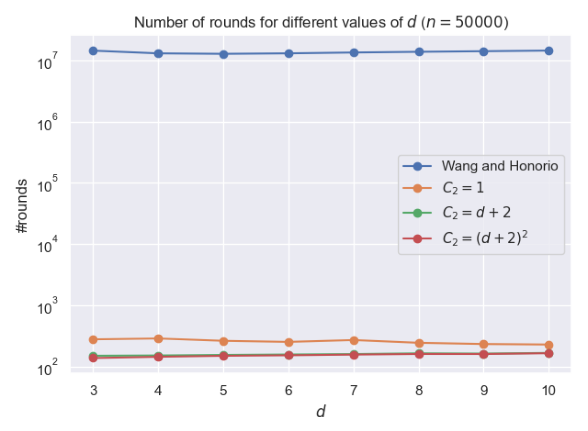
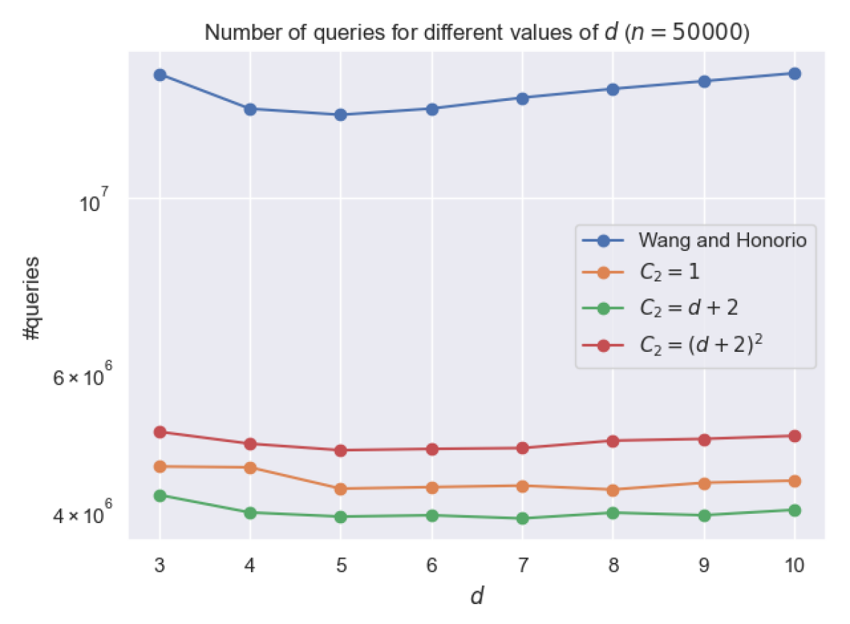
Figure 11: Comparing our algorithm’s number of rounds (left) and total queries (right) with Wang and Honorio’s [45], for $n=50000$ and varying values for $d$.

In Figure 11, we compare Algorithm 3 with the one by Wang and Honorio [45] for fixed size and varying values of $d$. Again, this supports our theoretical findings that our algorithm achieves both a significant parallel speedup and a simultaneous improvement in the number of total queries.

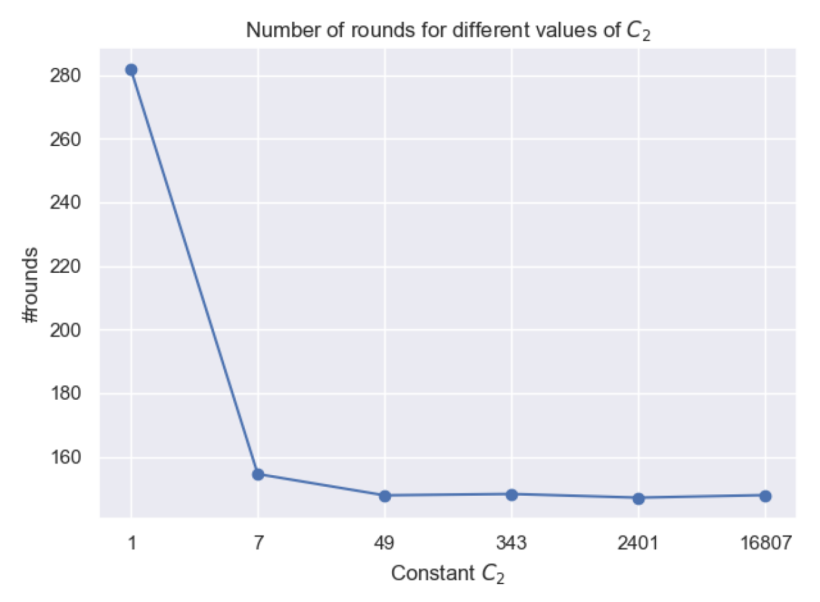
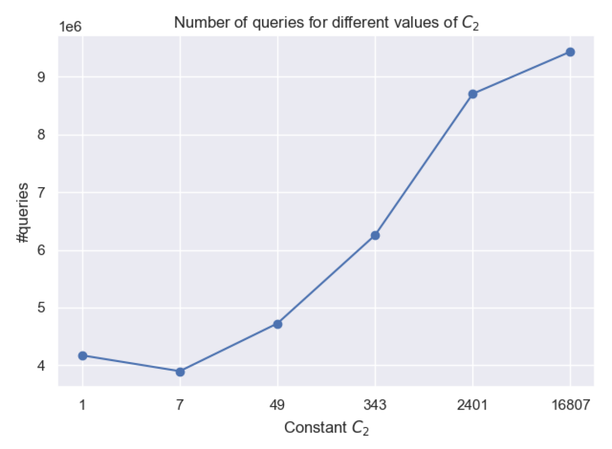
Figure 12: Change in the total number of rounds (left) and total number of queries (right) when running our algorithm for varying values of $C_{2}$ ($n=50000$, $d=5$).

In Figure 12, we study the behavior of Algorithm 3 under different values of $C_{2}$, so as to experimentally find the best value for $C_{2}$. While our high probability analysis requires $C_{2}\approx(d+2)^{4}$, Figure 12 suggests that we do not need that high probability reassurance in practice, and we can use smaller sample to reduce the total number of queries.

Real Data.

Our experiments on real-world biological phylogenetic trees also confirm the superiority of our algorithm in terms of performance as compared to the one by Wang and Honorio [45]. Similar to our experiments using relative-distance queries, we used a dataset comprised of trees from the phylogenetic library TreeBase [35]. Figure 13 summarizes our experimental results, where each data point corresponds to an average performance of 3 runs on the same tree. Our algorithm is superior in both queries and rounds for all the values of $C_{2}$ we tried: $C_{2}\in\{1,d+2,(d+2)^{2}\}$. The best performance corresponds to $C_{2}=d+2=5$, which is the one illustrated in Figure 13.

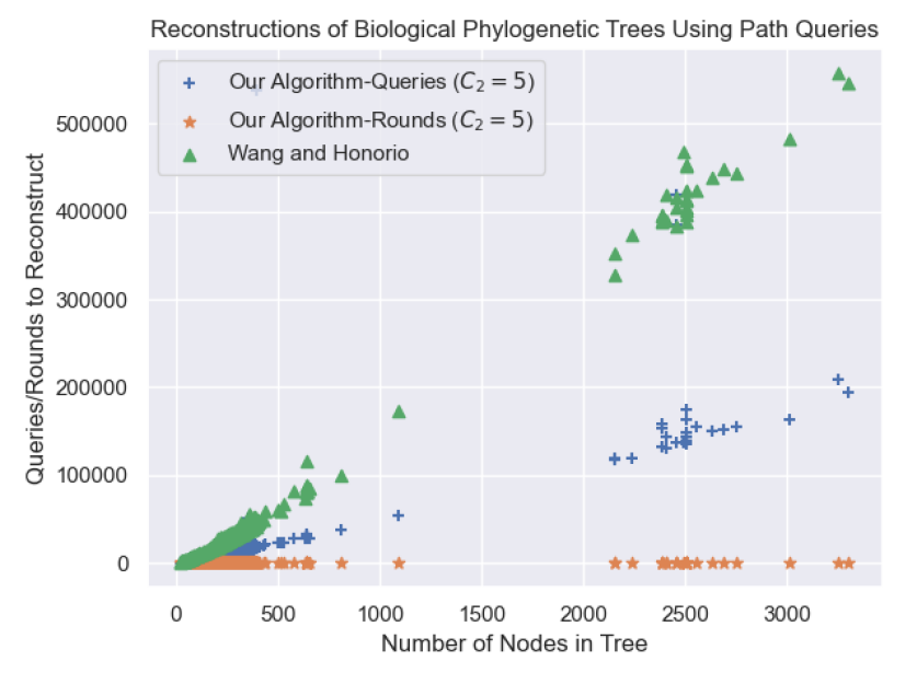
Figure 13: A scatter plot comparing the number of queries and rounds of our algorithm and with the one by Wang and Honorio [45] for real-world trees from TreeBase [35]. Since our algorithm is parallel, we include round complexity to serve as a comparison for the sequential complexity.

Appendix A Probabilistic Analysis for Tree Reconstruction using Path Queries

Here, we give the Chernoff-bound analysis that we omitted in the proof of lemma 4.12.

Lemma A.1.

There exists a constant $C_{2}>0$, as used $K=C_{2}\log{|V|}$in line 4 of Algorithm 4, such that if we take a sample $X$ of size $K$ from $V$, the following probability bounds always hold:

$$\begin{cases}\Pr\left(count(s,X)\geq\frac{K}{d+1}\right)\geq 1-\frac{1}{|V|^{2}}&\mbox{if }count(s,V)\geq\frac{|V|}{d},\\ \Pr\left(count(s,X)\leq K\frac{d}{d+1}\right)\geq 1-\frac{1}{|V|^{2}}&\mbox{if }count(s,V)\leq|V|\frac{d-1}{d},\\ \end{cases}$$ (1)

$$\begin{cases}\Pr\left(count(s,X)<\frac{K}{d+1}\right)\geq 1-\frac{1}{|V|^{2}}&\mbox{if }count(s,V)<\frac{|V|}{d+2},\\ \Pr\left(count(s,X)>K\frac{d}{d+1}\right)\geq 1-\frac{1}{|V|^{2}}&\mbox{if }count(s,V)>|V|\frac{d+1}{d+2}\\ \end{cases}$$ (2)

Proof A.2.

Recall that $\tilde{D}(s)=count(s,X)\frac{|V|}{K}$ is an estimation of $D(s)=count(s,V)$, the number of descendants of vertex $s$ in algorithm 4. For simplicity, we use $D(s)$ and $\tilde{D}(s)$ in the proof. Let $Z$ be sum of independent binary random variables with expected value $E[Z]$. Using a Chernoff bound, we know that $\Pr\left[\big{|}Z-E[Z]\big{|}\geq\epsilon E[Z]\right]\leq 2e^{\frac{-1}{3}\epsilon^{2}E[Z]}$:

In this case, our random variable is $Z=\tilde{D}(s)\frac{K}{|V|}$ and $E[Z]=D(s)\frac{K}{|V|}$. By reformulating a Chernoff bound, we have

$$\Pr\left[\big{|}Z-D(s)\frac{K}{|V|}\big{|}\geq\epsilon D(s)\frac{K}{|V|}\right]\leq 2e^{\frac{-1}{3}\epsilon^{2}D(s)\frac{K}{|V|}}$$ (3)

Now, we find the value of $C_{2}$ used in line 4 of algorithm 4 to compute $K$, the size of the sample. We do this for each of the 4 cases distinguished in equations 2,3:

Case 1: We want to prove that if $D(s)\geq\frac{|V|}{d}$,

then $\Pr\left[\tilde{D}(s)\geq\frac{|V|}{(d+1)}\right]\geq 1-\frac{1}{|V|^{2}}$:

Suppose $D(s)\geq\frac{|V|}{d}$; we prove that $\Pr\left[\tilde{D}(s)<\frac{|V|}{d+1}\right]<\frac{1}{|V|^{2}}$.

If we set $\epsilon=\frac{1}{d+1}$, we show that

$$\Pr\left[\tilde{D}(s)<\frac{|V|}{d+1}\right]\leq\Pr\left[\left|Z-D(s)\frac{K}{|V|}\right|\geq\epsilon D(s)\frac{K}{|V|}\right]$$ (4)

In order to prove this, given the facts that $\epsilon=\frac{1}{d+1}$, and $D(s)\geq\frac{|V|}{d}$, we show that, for any $\tilde{D}(s)$ such that the inequality $\tilde{D}(s)<\frac{|V|}{d+1}$ holds, then the inequality $\left[\left|Z-D(s)\frac{K}{|V|}\right|\geq\epsilon D(s)\frac{K}{|V|}\right]$ also holds.

$$\frac{d}{d+1}D(s)\frac{K}{|V|}\geq\frac{K}{d+1}>Z \left(D(s)\geq\frac{|V|}{d},Z<\frac{K}{d+1}\right)$$

$$\Longrightarrow \left[\left(1-\frac{1}{d+1}\right)\left(D(s)\frac{K}{|V|}\right)\geq Z\right]$$

$$\Longrightarrow \left[\left(D(s)\frac{K}{|V|}-Z\right)\geq\frac{1}{d+1}D(s)\frac{K}{|V|}\right]$$

$$\Longrightarrow \left[\left|Z-D(s)\frac{K}{|V|}\right|\geq\epsilon D(s)\frac{K}{|V|}\right] \left(\epsilon=\frac{1}{d+1}\right)$$

Thus, inequality 4 is true. Combining inequalities 3 and 4, we have that:

$$\Pr\left[\tilde{D}(s)<\frac{|V|}{d+1}\right]\leq 2e^{\frac{-1}{3}\epsilon^{2}D(s)\frac{K}{|V|}}$$

Now, we find the value of $C_{2}$, such that for $K=C_{2}\log{|V|}$:

$$2e^{\frac{-1}{3}\epsilon^{2}D(s)\frac{K}{|V|}}<\frac{1}{|V|^{2}}$$

Taking logarithm on both sides and given that $D(s)\geq\frac{|V|}{d}$ and $\epsilon=\frac{1}{d+1}$, we have that:

$$\frac{1}{3}\epsilon^{2}D(s)\frac{K}{|V|}\geq\frac{1}{3}\left(\frac{1}{d+1}\right)^{2}\frac{|V|}{|d|}\frac{K}{|V|}=\frac{1}{3}\left(\frac{1}{d+1}\right)^{2}\frac{K}{d}>2\ln{(2|V|)}$$

$$\Longleftrightarrow K>6d(d+1)^{2}\ln{(2|V|)}$$

$$\xLongleftrightarrow{K=C_{2}\log{|V|}}C_{2}>\frac{6d(d+1)^{2}\ln{(2|V|)}}{\log{|V|}}$$

Thus, $C_{2}$ is not more than a constant.

Case 2: We want to prove that if $D(s)\leq\frac{|V|(d-1)}{d}$,

then $\Pr\left[\tilde{D}(s)\leq\frac{|V|d}{(d+1)}\right]\geq 1-\frac{1}{|V|^{2}}$:

Suppose $D(s)\leq\frac{|V|(d-1)}{d}$; we prove that $\Pr\left[\tilde{D}(s)>\frac{|V|d}{(d+1)}\right]<\frac{1}{|V^{2}}$.

Reminding that $Z=\tilde{D}(s)\frac{K}{|V|}$, if we set $\epsilon=\frac{K}{d(d+1)E[Z]}$, we show:

$$\Pr\left[\tilde{D}(s)>\frac{\left|V\right|d}{\left(d+1\right)}\right]\leq\Pr\left[\left|Z-D(s)\frac{K}{|V|}\right|\geq\epsilon D(s)\frac{K}{|V|}\right]$$ (5)

In order to prove this, given the facts that $\epsilon=\frac{K}{d(d+1)E[Z]}$, and $D(s)\leq\frac{|V|\left(d-1\right)}{d}$, we show that, for any $\tilde{D}(s)$ such that the inequality $Z=\tilde{D}(s)\frac{K}{|V|}>\frac{Kd}{d+1}$ holds, then the inequality $\left[\left|Z-D(s)\frac{K}{|V|}\right|\geq\epsilon D(s)\frac{K}{|V|}\right]$ also holds.

Given that $Z>\frac{Kd}{d+1}$ and that $D(s)\leq\frac{|V|\left(d-1\right)}{d}$, we have:

$$\left|Z-D(s)\frac{K}{|V|}\right|=\left(Z-D(s)\frac{K}{|V|}\right)$$

$$>\frac{Kd}{d+1}-\frac{|V|\left(d-1\right)}{d}\frac{K}{|V|}=\frac{K}{d\left(d+1\right)}$$

Therefore, using the facts that $\epsilon=\frac{K}{d\left(d+1\right)E[Z]}$ and that $E[Z]=D(s)\frac{K}{|V|}$, we can say:

$$\left|Z-D(s)\frac{K}{|V|}\right|\geq\epsilon D(s)\frac{K}{|V|}$$

Thus, inequality 5 is true. Combining inequalities 3 and 5, we have:

$$\Pr\left[\tilde{D}(s)>\frac{|V|d}{\left(d+1\right)}\right]\leq 2e^{\frac{-1}{3}\epsilon^{2}D(s)\frac{K}{|V|}}$$

Now, we find the value of $C_{2}$, such that for $K=C_{2}\log{|V|}$:

$$2e^{\frac{-1}{3}\epsilon^{2}D(s)\frac{K}{|V|}}<\frac{1}{|V|^{2}}$$

Taking logarithm on both sides and given that $\epsilon E[Z]=\frac{K}{d(d+1)}$ and $E[Z]=D(s)\frac{K}{|V|}\leq\frac{K(d-1)}{d}$, we can obtain $\epsilon\geq\frac{1}{(d-1)(d+1)}$, therefore:

$$\frac{1}{3}\epsilon^{2}D(s)\frac{K}{|V|}\geq\frac{1}{3}\frac{1}{(d-1)(d+1)}\frac{|K|}{d(d+1)}>2\ln{(2|V|)}$$

$$\Longleftrightarrow K>6d(d-1)(d+1)^{2}\ln{(2|V|)}$$

$$\xLongleftrightarrow{K=C_{2}\log{|V|}}C_{2}>\frac{6d\dot{(}d-1)(d+1)^{2}\ln{(2|V|)}}{\log{|V|}}$$

Thus, $C_{2}$ is not more than a constant.

Case 3: We want to show that if $D(s)<\frac{|V|}{d+2}$,

then $\Pr\left[\tilde{D}(s)<\frac{|V|}{(d+1)}\right]\geq 1-\frac{1}{|V|^{2}}$:

Suppose $D(s)<\frac{|V|}{d+2}$; we prove that $\Pr\left[\tilde{D}(s)\geq\frac{|V|}{d+1}\right]<\frac{1}{|V|^{2}}$.

Reminding that $Z=\tilde{D}(s)\frac{K}{|V|}$, if we set $\epsilon=\frac{K}{(d+1)(d+2)E[Z]}$, we show:

$$\Pr\left[\tilde{D}(s)\geq\frac{\left|V\right|}{d+1}\right]\leq\Pr\left[\left|Z-D(s)\frac{K}{|V|}\right|\geq\epsilon D(s)\frac{K}{|V|}\right]$$ (6)

In order to prove this, given the facts that $\epsilon=\frac{K}{(d+1)(d+2)E[Z]}$, and $D(s)<\frac{|V|}{d+2}$ , we show that, for any $\tilde{D}(s)$ such that the inequality $Z=\tilde{D}(s)\frac{K}{|V|}\geq\frac{K}{d+1}$ holds, then the inequality $\left[\left|Z-D(s)\frac{K}{|V|}\right|\geq\epsilon D(s)\frac{K}{|V|}\right]$ also holds.

Given that $Z\geq\frac{K}{d+1}$ and that $D(s)<\frac{|V|}{d+2}$, we can say:

$$\left|Z-D(s)\frac{K}{|V|}\right|=\left(Z-D(s)\frac{K}{|V|}\right)$$

$$>\frac{K}{d+1}-\frac{|V|}{d+2}\frac{K}{|V|}=\frac{K}{\left(d+1\right)\left(d+2\right)}$$

Therefore, using the facts that $\epsilon=\frac{K}{\left(d+1\right)\left(d+2\right)E[Z]}$ and that $E[Z]=D(s)\frac{K}{|V|}$, we have:

$$\left|Z-D(s)\frac{K}{|V|}\right|\geq\epsilon D(s)\frac{K}{|V|}$$

Thus, inequality 6 is true. Combining inequalities 3 and 6, we can say:

$$\Pr\left[\tilde{D}(s)\geq\frac{|V|}{d+1}\right]\leq 2e^{\frac{-1}{3}\epsilon^{2}D(s)\frac{K}{|V|}}$$

Now, we find the value of $C_{2}$, such that for $K=C_{2}\log{|V|}$:

$$2e^{\frac{-1}{3}\epsilon^{2}D(s)\frac{K}{|V|}}<\frac{1}{|V|^{2}}$$

Taking logarithm on both sides and given that

$\epsilon E[Z]=\frac{K}{(d+1)(d+2)}$ and $E[Z]=D(s)\frac{K}{|V|}<\frac{K}{d+2}$, we can obtain $\epsilon>\frac{1}{(d+1)}$, therefore:

$$\frac{1}{3}\epsilon^{2}D(s)\frac{K}{|V|}\geq\frac{1}{3}\frac{1}{(d+1)}\frac{|K|}{(d+2)(d+1)}>2\ln{(2|V|)}$$

$$\Longleftrightarrow K>6(d+2)(d+1)^{2}\ln{(2|V|)}$$

$$\xLongleftrightarrow{K=C_{2}\log{|V|}}C_{2}>\frac{6(d+2)(d+1)^{2}\ln{(2|V|)}}{\log{|V|}}$$

Thus, $C_{2}$ is not more than a constant.

Case 4: We want to prove that if $D(s)>\frac{|V|(d+1)}{d+2}$,

then $\Pr\left[\tilde{D}(s)>\frac{|V|d}{(d+1)}\right]\geq 1-\frac{1}{|V|^{2}}$:

Suppose $D(s)>\frac{|V|(d+1)}{d+2}$; we prove that $\Pr\left[\tilde{D}(s)\leq\frac{|V|d}{(d+1)}\right]\geq 1-\frac{1}{|V|^{2}}$.

Reminding that $Z=\tilde{D}(s)\frac{K}{|V|}$, if we set $\epsilon=\frac{K}{(d+1)(d+2)E[Z]}$, we show:

$$\Pr\left[\tilde{D}(s)\leq\frac{|V|d}{(d+1)}\right]\leq\Pr\left[\left|X-D(s)\frac{K}{|V|}\right|\geq\epsilon D(s)\frac{K}{|V|}\right]$$ (7)

In order to prove this, given the facts that $\epsilon=\frac{K}{(d+1)(d+2)E[Z]}$, and $D(s)>\frac{|V|\left(d+1\right)}{d+2}$ , we show that, for any $\tilde{D}(s)$ such that the inequality $Z=\tilde{D}(s)\frac{K}{|V|}\leq\frac{Kd}{d+1}$ holds, then the inequality $\left[\left|Z-D(s)\frac{K}{|V|}\right|\geq\epsilon D(s)\frac{K}{|V|}\right]$ also holds.

Given that $Z\leq\frac{Kd}{d+1}$ and that $D(s)>\frac{|V|(d+1)}{d+2}$, we can say:

$$\left|X-D(s)\frac{K}{|V|}\right|=\left(D(s)\frac{K}{|V|}-Z\right)$$

$$>\frac{|V|(d+1)}{d+2}\frac{K}{|V|}-\frac{Kd}{d+1}=\frac{K}{\left(d+1\right)\left(d+2\right)}$$

Therefore, using the facts that $\epsilon=\frac{K}{\left(d+1\right)\left(d+2\right)E[Z]}$ and that $E[Z]=D(s)\frac{K}{|V|}$, we have:

$$\left|Z-D(s)\frac{K}{|V|}\right|\geq\epsilon D(s)\frac{K}{|V|}$$

Thus, inequality 7 is true. Combining inequalities 3 and 7, we can see:

$$\Pr\left[\tilde{D}(s)\leq\frac{|V|d}{(d+1)}\right]\leq 2e^{\frac{-1}{3}\epsilon^{2}D(s)\frac{K}{|V|}}$$

Now, we find the value of $C_{2}$, such that for $K=C_{2}\log{|V|}$:

$$2e^{\frac{-1}{3}\epsilon^{2}D(s)\frac{K}{|V|}}<\frac{1}{|V|^{2}}$$

Taking logarithm on both sides and given that

$\epsilon E[Z]=\frac{K}{(d+1)(d+2)}$ and $E[Z]=D(s)\frac{K}{|V|}\leq K$, we can obtain $\epsilon\geq\frac{1}{(d+1)(d+2)}$, therefore:

$$\frac{1}{3}\epsilon^{2}D(s)\frac{K}{|V|}\geq\frac{1}{3}\frac{1}{(d+1)(d+2)}\frac{|K|}{(d+2)(d+1)}>2\ln{(2|V|)}$$

$$\Longleftrightarrow K>6(d+2)^{2}(d+1)^{2}\ln{(2|V|)}$$

$$\xLongleftrightarrow{K=C_{2}\log{|V|}}C_{2}>\frac{6(d+2)^{2}(d+1)^{2}\ln{(2|V|)}}{\log{|V|}}$$

Thus, $C_{2}$ is not more than a constant.

Therefore, it’s enough to choose $C_{2}$ as the maximum of these 4 constants at the beginning of the algorithm.

References

- [1] Peyman Afshani, Manindra Agrawal, Benjamin Doerr, Carola Doerr, Kasper Green Larsen, and Kurt Mehlhorn. The query complexity of finding a hidden permutation. In Andrej Brodnik, Alejandro López-Ortiz, Venkatesh Raman, and Alfredo Viola, editors, Space-Efficient Data Structures, Streams, and Algorithms - Papers in Honor of J. Ian Munro on the Occasion of His 66th Birthday, volume 8066 of Lecture Notes in Computer Science, pages 1–11. Springer, 2013. doi:10.1007/978-3-642-40273-9\_1.
- [2] Ramtin Afshar, Michael T. Goodrich, Pedro Matias, and Martha C. Osegueda. Reconstructing binary trees in parallel. In Christian Scheideler and Michael Spear, editors, SPAA ’20: 32nd ACM Symposium on Parallelism in Algorithms and Architectures, Virtual Event, USA, July 15-17, 2020, pages 491–492. ACM, 2020. doi:10.1145/3350755.3400229.
- [3] Gautam Altekar, Sandhya Dwarkadas, John P. Huelsenbeck, and Fredrik Ronquist. Parallel metropolis coupled markov chain monte carlo for bayesian phylogenetic inference. Bioinform., 20(3):407–415, 2004. doi:10.1093/bioinformatics/btg427.
- [4] Anna Bernasconi, Carsten Damm, and Igor E. Shparlinski. Circuit and decision tree complexity of some number theoretic problems. Inf. Comput., 168(2):113–124, 2001. doi:10.1006/inco.2000.3017.
- [5] Paolo Bestagini, Marco Tagliasacchi, and Stefano Tubaro. Image phylogeny tree reconstruction based on region selection. In 2016 IEEE International Conference on Acoustics, Speech and Signal Processing, ICASSP 2016, Shanghai, China, March 20-25, 2016, pages 2059–2063. IEEE, 2016. doi:10.1109/ICASSP.2016.7472039.
- [6] Anupam Bhattacharjee, Kazi Zakia Sultana, and Zalia Shams. Dynamic and parallel approaches to optimal evolutionary tree construction. In Proceedings of the Canadian Conference on Electrical and Computer Engineering, CCECE 2006, May 7-10, 2006, Ottawa Congress Centre, Ottawa, Canada, pages 119–122. IEEE, 2006. doi:10.1109/CCECE.2006.277582.
- [7] Gerth Stølting Brodal, Rolf Fagerberg, Christian N. S. Pedersen, and Anna Östlin. The complexity of constructing evolutionary trees using experiments. In Fernando Orejas, Paul G. Spirakis, and Jan van Leeuwen, editors, Automata, Languages and Programming, 28th International Colloquium, ICALP 2001, Crete, Greece, July 8-12, 2001, Proceedings, volume 2076 of Lecture Notes in Computer Science, pages 140–151. Springer, 2001. doi:10.1007/3-540-48224-5\_12.
- [8] Sung-Soon Choi and Jeong Han Kim. Optimal query complexity bounds for finding graphs. Artif. Intell., 174(9-10):551–569, 2010. doi:10.1016/j.artint.2010.02.003.
- [9] Benny Chor and Tamir Tuller. Maximum likelihood of evolutionary trees: hardness and approximation. In Proceedings Thirteenth International Conference on Intelligent Systems for Molecular Biology 2005, Detroit, MI, USA, 25-29 June 2005, pages 97–106, 2005. doi:10.1093/bioinformatics/bti1027.
- [10] Richard Cole and Uzi Vishkin. Deterministic coin tossing and accelerating cascades: micro and macro techniques for designing parallel algorithms. In Juris Hartmanis, editor, Proceedings of the 18th Annual ACM Symposium on Theory of Computing, May 28-30, 1986, Berkeley, California, USA, pages 206–219. ACM, 1986. doi:10.1145/12130.12151.
- [11] Thomas H. Cormen, Charles E. Leiserson, Ronald L. Rivest, and Clifford Stein. Introduction to Algorithms, 3rd Edition. MIT Press, 2009. URL: http://mitpress.mit.edu/books/introduction-algorithms.
- [12] Joseph C. Culberson and Piotr Rudnicki. A fast algorithm for constructing trees from distance matrices. Inf. Process. Lett., 30(4):215–220, 1989. doi:10.1016/0020-0190(89)90216-0.
- [13] Zanoni Dias, Siome Goldenstein, and Anderson Rocha. Exploring heuristic and optimum branching algorithms for image phylogeny. J. Vis. Commun. Image Represent., 24(7):1124–1134, 2013. doi:10.1016/j.jvcir.2013.07.011.
- [14] Zanoni Dias, Siome Goldenstein, and Anderson Rocha. Large-scale image phylogeny: Tracing image ancestral relationships. IEEE Multim., 20(3):58–70, 2013. doi:10.1109/MMUL.2013.17.
- [15] Zanoni Dias, Anderson Rocha, and Siome Goldenstein. Image phylogeny by minimal spanning trees. IEEE Trans. Information Forensics and Security, 7(2):774–788, 2012. doi:10.1109/TIFS.2011.2169959.
- [16] Shahar Dobzinski and Jan Vondrák. From query complexity to computational complexity. In Howard J. Karloff and Toniann Pitassi, editors, Proceedings of the 44th Symposium on Theory of Computing Conference, STOC 2012, New York, NY, USA, May 19 - 22, 2012, pages 1107–1116. ACM, 2012. doi:10.1145/2213977.2214076.
- [17] Ehsan Emamjomeh-Zadeh and David Kempe. Adaptive hierarchical clustering using ordinal queries. In Artur Czumaj, editor, Proceedings of the Twenty-Ninth Annual ACM-SIAM Symposium on Discrete Algorithms, SODA 2018, New Orleans, LA, USA, January 7-10, 2018, pages 415–429. SIAM, 2018. doi:10.1137/1.9781611975031.28.
- [18] James S. Farris. Methods for Computing Wagner Trees. Systematic Biology, 19(1):83–92, 03 1970. arXiv:https://academic.oup.com/sysbio/article-pdf/19/1/83/4642459/19-1-83.pdf, doi:10.1093/sysbio/19.1.83.
- [19] Joseph Felsenstein. Evolutionary trees from dna sequences: a maximum likelihood approach. Journal of molecular evolution, 17(6):368–376, 1981.
- [20] Walter M. Fitch. Toward defining the course of evolution: Minimum change for a specific tree topology. Systematic Zoology, 20(4):406–416, 1971. URL: http://www.jstor.org/stable/2412116.
- [21] Leslie Ann Goldberg, Paul W. Goldberg, Cynthia A. Phillips, and Gregory B. Sorkin. Constructing computer virus phylogenies. J. Algorithms, 26(1):188–208, 1998. doi:10.1006/jagm.1997.0897.
- [22] M. T. Goodrich and R. Tamassia. Algorithm Design and Applications. Wiley, New York, NY, 2011.
- [23] Jotun J Hein. An optimal algorithm to reconstruct trees from additive distance data. Bulletin of mathematical biology, 51(5):597–603, 1989.
- [24] John P Huelsenbeck. Performance of phylogenetic methods in simulation. Systematic biology, 44(1):17–48, 1995.
- [25] M. Jagadish and Anindya Sen. Learning a bounded-degree tree using separator queries. In Sanjay Jain, Rémi Munos, Frank Stephan, and Thomas Zeugmann, editors, Algorithmic Learning Theory - 24th International Conference, ALT 2013, Singapore, October 6-9, 2013. Proceedings, volume 8139 of Lecture Notes in Computer Science, pages 188–202. Springer, 2013. doi:10.1007/978-3-642-40935-6\_14.
- [26] Jeong-Hoon Ji, Su-Hyun Park, Gyun Woo, and Hwan-Gue Cho. Generating pylogenetic tree of homogeneous source code in a plagiarism detection system. International Journal of Control, Automation, and Systems, 6(6):809–817, 2008.
- [27] Neil C Jones, Pavel A Pevzner, and Pavel Pevzner. An introduction to bioinformatics algorithms. MIT press, 2004.
- [28] Sampath Kannan, Eugene L. Lawler, and Tandy J. Warnow. Determining the evolutionary tree using experiments. J. Algorithms, 21(1):26–50, 1996. doi:10.1006/jagm.1996.0035.
- [29] Sampath Kannan, Claire Mathieu, and Hang Zhou. Graph reconstruction and verification. ACM Trans. Algorithms, 14(4):40:1–40:30, 2018. doi:10.1145/3199606.
- [30] Valerie King, Li Zhang, and Yunhong Zhou. On the complexity of distance-based evolutionary tree reconstruction. In Proceedings of the Fourteenth Annual ACM-SIAM Symposium on Discrete Algorithms, January 12-14, 2003, Baltimore, Maryland, USA, pages 444–453. ACM/SIAM, 2003. URL: http://dl.acm.org/citation.cfm?id=644108.644179.
- [31] Guilherme D Marmerola, Marina A Oikawa, Zanoni Dias, Siome Goldenstein, and Anderson Rocha. On the reconstruction of text phylogeny trees: evaluation and analysis of textual relationships. PloS one, 11(12):e0167822, 2016.
- [32] Michael Mitzenmacher and Eli Upfal. Probability and Computing: Randomized Algorithms and Probabilistic Analysis. Cambridge University Press, 2005. doi:10.1017/CBO9780511813603.
- [33] Mark Pagel. Inferring the historical patterns of biological evolution. Nature, 401(6756):877–884, 1999.
- [34] Avi Pfeffer, Catherine Call, John Chamberlain, Lee Kellogg, Jacob Ouellette, Terry Patten, Greg Zacharias, Arun Lakhotia, Suresh Golconda, John Bay, Robert Hall, and Daniel Scofield. Malware analysis and attribution using genetic information. In 7th International Conference on Malicious and Unwanted Software, MALWARE 2012, Fajardo, PR, USA, October 16-18, 2012, pages 39–45. IEEE Computer Society, 2012. doi:10.1109/MALWARE.2012.6461006.
- [35] WH Piel, L Chan, MJ Dominus, J Ruan, RA Vos, and V Tannen. Treebase v. 2: A database of phylogenetic knowledge. e-biosphere, 2009.
- [36] Heinz Prüfer. Neuer beweis eines satzes über permutationen. Arch. Math. Phys, 27(1918):742–744, 1918.
- [37] Lev Reyzin and Nikhil Srivastava. On the longest path algorithm for reconstructing trees from distance matrices. Inf. Process. Lett., 101(3):98–100, 2007. doi:10.1016/j.ipl.2006.08.013.
- [38] F. James Rohlf. J. felsenstein, inferring phylogenies, sinauer assoc., 2004, pp. xx + 664. J. Classif., 22(1):139–142, 2005. doi:10.1007/s00357-005-0009-4.
- [39] Bingyu Shen, Christopher W. Forstall, Anderson de Rezende Rocha, and Walter J. Scheirer. Practical text phylogeny for real-world settings. IEEE Access, 6:41002–41012, 2018. doi:10.1109/ACCESS.2018.2856865.
- [40] Yossi Shiloach and Uzi Vishkin. Finding the maximum, merging and sorting in a parallel computation model. In Wolfgang Händler, editor, CONPAR 81: Conference on Analysing Problem Classes and Programming for Parallel Computing, Nürnberg, Germany, June 10-12, 1981, Proceedings, volume 111 of Lecture Notes in Computer Science, pages 314–327. Springer, 1981. doi:10.1007/BFb0105127.
- [41] Gábor Tardos. Query complexity, or why is it difficult to seperate NP cap co np from p by random oracles a? Combinatorica, 9(4):385–392, 1989. doi:10.1007/BF02125350.
- [42] W.T. Tutte. Graph Theory. Cambridge Mathematical Library. Cambridge University Press, 2001. URL: https://books.google.com/books?id=uTGhooU37h4C.
- [43] Leslie G. Valiant. Parallelism in comparison problems. SIAM J. Comput., 4(3):348–355, 1975. doi:10.1137/0204030.
- [44] Leslie G. Valiant. Universality considerations in VLSI circuits. IEEE Trans. Computers, 30(2):135–140, 1981. doi:10.1109/TC.1981.6312176.
- [45] Zhaosen Wang and Jean Honorio. Reconstructing a bounded-degree directed tree using path queries. In 57th Annual Allerton Conference on Communication, Control, and Computing, Allerton 2019, Monticello, IL, USA, September 24-27, 2019, pages 506–513. IEEE, 2019. doi:10.1109/ALLERTON.2019.8919924.
- [46] Michael S Waterman, Temple F Smith, Mona Singh, and William A Beyer. Additive evolutionary trees. Journal of theoretical Biology, 64(2):199–213, 1977.
- [47] Andrew Chi-Chih Yao. Decision tree complexity and betti numbers. In Frank Thomson Leighton and Michael T. Goodrich, editors, Proceedings of the Twenty-Sixth Annual ACM Symposium on Theory of Computing, 23-25 May 1994, Montréal, Québec, Canada, pages 615–624. ACM, 1994. doi:10.1145/195058.195414.