A shell-model study of calcium isotopes towards their drip line

Abstract

We report in this paper a study in terms of the nuclear shell model about the location of the calcium isotopes drip line. The starting point is considering the realistic two-body potential derived by Entem and Machleidt within chiral perturbation theory at next-to-next-to-next-to-leading order (N³LO), as well as a chiral three-body force at next-to-next-to-leading order (N²LO) whose structure and low-energy constants are consistent with the two-body potential. Then we construct the effective single-particle energies and residual interaction needed to diagonalize the shell-model Hamiltonian. The calculated two-neutron separation energies agree nicely with experiment until ⁵⁶Ca, which is the heaviest isotope whose mass has been measured, and do not show any sign of two-neutron emission until ⁷⁰Ca. We discuss the role of the choice of the model space in determining the neutron drip line, and also the dependence of the results on the parameters of the shell-model Hamiltonian.

I Introduction

The location of the boundaries of the nuclear landscape is an important target in order to understand the limits of the strong force to hold together the nucleons in a bound system.

The search of drip lines is not an easy task from the experimental point of view, due to the extremely low production rates in investigations dealing with the fragmentation of stable nuclei, and the subsequent separation and identification of the products. This is why the possibility of expanding the chart of nuclides is closely linked to the development of facilities providing a new generation of re-accelerated radioactive ion beams as well as of new instrumentation and advanced techniques (see, for example, Ref. Thoennesen (2013)). Consequently, theory is in charge to provide further insight on this topic, and also to look for useful tips for experimental studies whose results may help to find evidence of proton/neutron drip lines.

In this context, calcium isotopes are one of the most intriguing subjects to be investigated, since this isotopic chain spans from the neutron-deficient ³⁶Ca, which lies close to the proton drip line, up to ⁶⁰Ca, that has been recently observed Tarasov et al. (2018) and whose $N/Z$ ratio, equal to 2, classifies it as a very exotic nuclear system. As a matter of fact, the observation of ⁶⁰Ca draws a line between studies predicting it as a loosely bound nucleus Meng et al. (2002); Hagen et al. (2012); Hergert et al. (2014) and those pushing neutron drip line up to ⁷⁰Ca Bhattacharya and Gangopadhyay (2005); Chen and Piekarewicz (2015); Cao et al. (2019); Neufcourt et al. (2019). Moreover, recent mass measurements of heavy calcium isotopes Wienholtz et al. (2013); Michimasa et al. (2018) are helpful to narrow the spread of the theoretical predictions about this yet undiscovered section of the chart of nuclides.

Another interesting aspect is the impulse that the novel experimental results have given to the advance in theory. In Ref. Neufcourt et al. (2019) the authors have followed an innovative approach to the study of calcium-isotopes drip line; they have performed a model averaging analysis of the outcome of different density-functional calculations, by way of Bayesian machine learning. The result of their study is that, by considering both experimental information and current density-functional models, ⁶⁸Ca owns an average posterior probability of about 76$\%$ to be bound with respect to the two-neutron emission. It is worth stressing that this study conjugates advances in computational theory - machine-learning methods - with a comparative analysis of energy-density functionals that are constrained to reproduce a variety of nuclear binding energies and radii.

Nuclei approaching the neutron drip line may show exotic features such as an extended neutron distribution and halo. This may be difficult to be reproduced with the harmonic-oscillator basis, since this could provide a slow convergence rate of the calculations. On the above grounds, the authors in Ref. Hagen et al. (2012) have investigated the evolution of shell structure of neutron-rich calcium isotopes by way of the coupled-cluster method, starting from chiral two- and three-body forces, and including the coupling to the particle continuum in terms of the Berggren basis.

The effects of a neutron skin have been studied in Ref. Hagen et al. (2013), where the neutron ⁶⁰Ca $S$-wave scattering phase shifts have been calculated within the coupled-cluster theory, employing interactions derived from chiral perturbation theory. The authors have found evidence of Efimov physics, namely a discrete scale invariance in three-body systems such as a tight core and two loosely bound nucleons Efimov (1970).

Neutron-halo features of neutron-rich calcium isotopes have been also investigated within the framework of the relativistic-mean-field and complex-momentum-representation method Cao et al. (2019), providing indications of a possible halo or giant halo structure of isotopes with $N\geq 40$.

Finally, it is also worth mentioning recent studies about the calcium isotopic chain by way of microscopic many-body approaches - and employing chiral two- and three-body potentials - such as the Bogoliubov many-body perturbation theory Tichai et al. (2018), the In-Medium Similarity Renormalization Group Simonis et al. (2017); Hoppe et al. (2019), and the Self-Consistent Green’s Function Theory Somà et al. (2020).

Our aim is to study heavy calcium isotopes, providing a prediction of their neutron drip line and shell evolution by way of nuclear shell model (SM). The framework is the same of our previous study about the monopole component of the shell-model Hamiltonian for $0f1p$-shell nuclei, where the single-particle (SP) energies and the two-body matrix elements (TBMEs) of the residual interaction have been derived from two- and three-body forces obtained by way of the chiral perturbation theory (ChPT) Ma et al. (2019). The main difference here is that we consider a larger model space, by including the neutron $0g_{9/2}$ orbital in addition to the $0f1p$ orbitals, a choice that is needed to extend the calculations to isotopes with $N>40$. We will focus on the relevance of the new SP degree of freedom, and of the induced three-body contributions that appear in the effective SM Hamiltonian $H_{\rm eff}$ to account for many-body correlations in nuclei with more than two valence nucleons Polls et al. (1983). This means that in the derivation of $H_{\rm eff}$we consider also the interaction of clusters of three-valence nucleons with core excitations as well as with virtual intermediate nucleons scattered above the model space, through density-dependent $H_{\rm eff}$s, whose TBMEs change according to the number of valence nucleons.

It should be pointed out that a similar approach has been followed by Holt and coworkers in Refs. Holt et al. (2012, 2014), where the two-body chiral potential has been renormalized through the $V_{{\rm low}\mbox{-}k}$ technique Bogner et al. (2002) and the effect of many-body correlations in the derivation of $H_{\rm eff}$has been neglected.

This paper is organized as follows: next section is devoted to present a few details of the derivation of the effective SM Hamiltonian from realistic two- and three-body nuclear potentials, that is framed within the many-body perturbation theory. In Section III the results of the diagonalization of the $H_{\rm eff}$s  for the calcium isotopic chain are presented and compared with available data from experiment. We will also show the results obtained previously within a smaller model space Ma et al. (2019), those obtained neglecting many-body correlations, and varying the energy of the $0g_{9/2}$ orbital, in order to provide insight on the sensitivity of SM results to the degrees of freedom our $H_{\rm eff}$s  account for. Finally, in Section IV we draw the conclusions of present investigation.

II Outline of calculations

II.1 The effective shell-model Hamiltonian

The SM parameters, that are needed to diagonalize the SM Hamiltonian, are derived from realistic nucleon-nucleon ($NN$) and three-body ($NNN$) potentials, both of them derived within the ChPT at next-to-next-to-next-to-leading order (N³LO) Entem and Machleidt (2002) and at next-to-next-to-leading order (N²LO), respectively. These potentials consistently share the same nonlocal regulator function, and some low-energy constants (LECs). More precisely, the N²LO $NNN$ potential is composed of three components, namely the two-pion ($2\pi$) exchange term $V_{3NF}^{(2\pi)}$, the one-pion ($1\pi$) exchange plus contact term $V_{3NF}^{(1\pi)}$, and the contact term $V_{3NF}^{\textrm{(ct)}}$. The $c_{1}$, $c_{3}$, and $c_{4}$ LECs which characterize these terms are the same as those in the N³LO $NN$ potential, and are determined by the renormalization procedure that is employed to fit the $NN$ data Machleidt and Entem (2011).

The values of the additional LECs appearing in 1$\pi$-exchange and contact terms of the $NNN$ potential, $c_{D}$ and $c_{E}$, have been chosen as $c_{D}=-1$ and $c_{E}=-0.34$. They have been determined in no-core shell model calculations Navrátil et al. (2007); Maris et al. (2013), by identifying a set of observables in light $p$-shell nuclei that are strongly sensitive to the $c_{D}$ value, and then $c_{E}$ has been constrained to reproduce the binding energies of the $A=3$ system.

In Appendix of Ref. Fukui et al. (2018), the details of the calculation of matrix elements of the N²LO $NNN$ potential, with a nonlocal regulator, in a harmonic-oscillator (HO) basis can be found.

The Coulomb potential is explicitly taken into account aside the matrix elements of the $NN$ potential. The oscillator parameter $\hbar\omega$ we have employed to compute the matrix elements of the $NN$ and $NNN$ potentials in the HO oscillator basis is equal to 11 MeV, according to the expression $\hbar\omega=45A^{-1/3}-25A^{-2/3}$ for $A=40$ Blomqvist and Molinari (1968).

These nuclear potentials are the foundations to build up the effective SM Hamiltonian $H_{\rm eff}$ that provides SP energies and TBMEs to solve the SM eigenvalue problem. As is well known, $H_{\rm eff}$ accounts for the degrees of freedom that are not explicitly included in the truncated Hilbert space of the configurations that, in our case, is spanned by four $0f1p$ plus $0g_{9/2}$ neutron orbitals outside the doubly-closed ⁴⁰Ca.

To this end, we need a similarity transformation which arranges, within the full Hilbert space of the configurations, a decoupling of the model space $P$ where the valence nucleons are constrained from its complement $Q=1-P$.

We tackle this problem within the time-dependent perturbation theory, namely $H_{\rm eff}$ is expressed through the Kuo-Lee-Ratcliff folded-diagram expansion in terms of the $\hat{Q}$-box vertex function Kuo and Osnes (1990); Hjorth-Jensen et al. (1995); Coraggio et al. (2012).

The $\hat{Q}$-box is defined in terms of the full nuclear Hamiltonian $H=H_{0}+H_{1}$, where $H_{0}$ is the unperturbed component and $H_{1}$ the interaction one:

$$\hat{Q}(\epsilon)=PH_{1}P+PH_{1}Q\frac{1}{\epsilon-QHQ}QH_{1}P~{},$$ (1)

and $\epsilon$ is an energy parameter called “starting energy”.

Since the exact calculation of the $\hat{Q}$-box is impossible, the term $1/(\epsilon-QHQ)$ is expanded as a power series

$$\frac{1}{\epsilon-QHQ}=\sum_{n=0}^{\infty}\frac{1}{\epsilon-QH_{0}Q}\left(\frac{QH_{1}Q}{\epsilon-QH_{0}Q}\right)^{n}~{},$$ (2)

leading to the perturbative expansion of the $\hat{Q}$-box. It is useful to employ a diagrammatic representation of this perturbative expansion, which is a collection of Goldstone diagrams that have at least one $H_{1}$-vertex, are irreducible - namely at least one line between two successive vertices does not belong to the model space - and are linked to at least one external valence line (valence linked) (Kuo et al., 1971).

Then, the $\hat{Q}$-box is employed to solve non-linear matrix equations to derive $H_{\rm eff}$  by way of iterative techniques such as the Kuo-Krenciglowa and Lee-Suzuki ones Suzuki and Lee (1980), or graphical non-iterative methods Suzuki et al. (2011). We have experienced that the latter provide a faster and more stable convergence to the solution of the matrix equation to derive $H_{\rm eff}$, and are the ones we have employed in present work.

We include in our $\hat{Q}$-box expansion one- and two-body Goldstone diagrams through third order in the $NN$ potential and up to first order in the $NNN$ one. A complete list of diagrams with $NN$ vertices can be found in Ref. Coraggio et al. (2012), while the diagrams at first order in $NNN$ potential, as well as their analytical expressions, are reported in Refs. Fukui et al. (2018); Ma et al. (2019). It is worth pointing out that these expressions are the coefficients of the one-body and two-body terms arising from the normal-ordering decomposition of the three-body component of a many-body Hamiltonian Hjorth-Jensen et al. (2017). In Ref. Holt et al. (2014), Holt and coworkers, using a similar approach to study Ca isotopes, have shown that the uncertainty linked to neglecting contributions beyond the normal-ordered two-body components (residual $NNN$ forces) is small.

Since we are going to study many-valence nucleon systems, we should derive many-body $H_{\rm eff}$s which depend on the number of valence particles. This means that the $\hat{Q}$-box should include at least contributions from three-body diagrams accounting for the interaction via the two-body force of the valence nucleons with configurations outside the model space.

Since we employ SM codes which cannot perform the diagonalization of a three-body $H_{\rm eff}$ Caurier et al. (2005); Shimizu et al. (2019), we derive a density-dependent two-body term from the three-body contribution arising at second order in perturbation theory. Namely, nine one-loop diagrams (see the graph $(b)$ in Fig. 1) are calculated from the corresponding diagrams reported in Fig. 3 of Ref. Polls et al. (1983).

Figure 1: Density-dependent two-body contribution that is obtained from a three-body one. Graph $(b)$ is obtained by summing over one incoming and outgoing particle of the three-body graph $(a)$.

Their explicit form is reported in Ref. Ma et al. (2019), and depends on the unperturbed occupation density $\rho_{m}$ of the orbital $j_{m}$, leading to the derivation of $H_{\rm eff}$s depending on the number of valence protons and neutrons. The density-dependent $H_{\rm eff}$s differ only in their TBMEs since, as can be seen in Fig. 1, these one-loop diagrams are two-body terms.

It should be recalled that, since the neutron $0g_{9/2}$ orbital may couple with the $0f_{7/2}$ one to the total angular momentum $J^{\pi}=1^{-}$, the results of the diagonalization of the shell-model Hamiltonian within the model space with 5 neutron orbitals might be affected somehow by the spurious center-of-mass motion Elliott and Skyrme (1955).

In order to check if these spuriosities are under control, we have also performed calculations to separate in energy the excitations originated by the internal degrees of freedom from those with spurious center-of-mass components by following the procedure suggested by Gloeckner and Lawson Gloeckner and Lawson (1974).

According to Ref. Gloeckner and Lawson (1974), the modified shell-model Hamiltonian $H^{\prime}$ should be diagonalized:

$$H^{\prime}=H_{\rm eff}+H_{\beta}~{}~{},$$ (3)

where $H_{\beta}$ is $\beta$ times the center-of-mass excitation energy of the $A$-nucleon system

$$H_{\beta}=\beta\left\{\frac{(\sum_{i=1}^{A}{\bf p_{i}})^{2}}{2Am}+\frac{m\omega^{2}}{2A}(\sum_{i=1}^{A}{\bf r_{i}})^{2}-\frac{3}{2}\hbar\omega\right\}~{}~{}.$$ (4)

The spurious components are then pushed up in energy by increasing the parameter $\beta$, so that one can assume that the low-energy spectrum is weakly influenced by the above components. We have performed calculations using values of $\beta$ such that $\gamma=\beta\frac{\hbar\omega}{A}$ is equal to 10 MeV and 15 MeV in order to evaluate the role of the center-of-mass spuriosities Liu et al. (2012), and the results will be reported in Section III.

II.2 Convergence properties of $H_{\rm eff}$

We now discuss the convergence properties of our $H_{\rm eff}$s, an issue that needs to be examined since the input chiral $NN$ and $NNN$ potentials have not been modified by way of any renormalization procedure.

In Ref. Ma et al. (2019) we have extensively discussed the order-by-order behavior of the perturbative expansion of the $\hat{Q}$-box, as well as the convergence with respect to the dimension of the space of the intermediate states, considering the systems with one- and two-valence neutrons, namely ⁴¹Ca and ⁴²Ca, respectively. We recall that we express the number of intermediate states as a function of the maximum allowed excitation energy of the intermediate states expressed in terms of the oscillator quanta $N_{\rm max}$ Coraggio et al. (2012), and include intermediate states with an unperturbed excitation energy up to $E_{\rm max}=N_{\rm max}\hbar\omega$. Because of our present limitation of the storage of the total number of TBMEs, we can include, for ⁴⁰Ca core, a maximum number of intermediate states that do not exceed $N_{\rm max}$=18.

In Ref. Ma et al. (2019), we have shown that this value is not large enough to provide convergence of the SP spectrum of ⁴¹Ca, since the chosen HO parameter is 11 MeV and the cutoff of both $NN$ and $NNN$ potentials is slightly larger than 2.5 fm^-1, this values leading to a value of $N_{\rm max}$ to be at least 26. However, this does not affect the convergence of the energy spacings that are stable with respect to the increase in the number of intermediate states from $N_{\rm max}\approx 12-14$ on for both ⁴¹Ca and ⁴²Ca, as already shown in Ref. Ma et al. (2019).

In this work we will show the convergence properties of $H_{\rm eff}$ by considering a more complex system, such as ⁵⁰Ca, which is characterized by 10 valence neutrons. By studying this system, we can test the perturbative behavior of $H_{\rm eff}$s that include density-dependent contributions which account for three-body correlations. It is worth pointing out that our choice is challenging, since ⁵⁰Ca exhibits a structure that is more collective than other neighbor isotopes, whose closure properties provide a simpler structure of the wave functions.

In Fig. 2 we report the low-lying states of ⁵⁰Ca spectrum, which have been obtained employing $H_{\rm eff}$s starting from $\hat{Q}$-boxes at first-, second-, and third-order in perturbation theory, and their Padé approximant $[2|1]$ Baker and Gammel (1970), while the number of intermediate states is the largest we can manage, i.e. $N_{\rm max}$=18.

We employ the Padé approximant in order to obtain a better estimate of the convergence value of the perturbation series Coraggio et al. (2012), as suggested in Ref. Hoffmann et al. (1976).

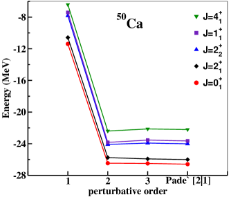
Figure 2: Low-lying energy spectrum of ⁵⁰Ca, obtained starting from $\hat{Q}$-boxes at first-, second-, and third-order in perturbation theory, and their Padé approximant $[2|1]$.

The results show a very satisfactory perturbative behavior of $H_{\rm eff}$ with respect to the order-by-order convergence.

We consider now the dependence of $H_{\rm eff}$ as a function of the number of intermediate states included in the calculation of the $\hat{Q}$-box second- and third-order diagrams.

As it as been mentioned before, $N_{\rm max}$=18 does not provide a convergent SP spectrum of ⁴¹Ca, but in Ref. Ma et al. (2019) we have shown that the SP spacings are stable. Consequently, from now on for our calculations we consider SP spacings obtained from the theory but the value of the SP energy of the neutron $0f_{7/2}$ orbital is fixed at -8.4 MeV, consistently with the experimental value in ⁴¹Ca Audi et al. (2003).

In Fig. 3 they are reported the energy spectra of ⁵⁰Ca, obtained diagonalizing the density-dependent $H_{\rm eff}$ calculated employing the Padé approximant $[2|1]$ of the $\hat{Q}$-box, and including a number of intermediates states ranging from $N_{\rm max}$=2 to 18. Theoretical results are also compared with experiment ens .

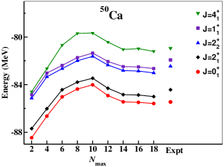
Figure 3: Low-lying energy spectrum of ⁵⁰Ca as a function of the number of intermediate states included in the perturbative calculation of the $\hat{Q}$-box.

Table 1: Theoretical proton ($\epsilon_{\pi}$) and neutron ($\epsilon_{\nu}$) SP energies (in MeV), referred to the $0f_{7/2}$ orbital.

	$\epsilon_{\pi}$	$\epsilon_{\nu}$
$0f_{7/2}$	0.0	0.0
$0f_{5/2}$	6.3	8.2
$1p_{3/2}$	2.5	3.2
$1p_{1/2}$	4.4	5.3
$0g_{9/2}$		9.9

This is a test for our theoretical SP spacings and, especially, TBMEs, and we observe that ⁵⁰Ca spectrum converges from $N_{\rm max}$=14 on. This leads to the conclusion that the SP spacings and TBMEs of our $H_{\rm eff}$, calculated with $N_{\rm max}$=18, can be considered substantially stable. It is worth pointing out that in Ref. Ma et al. (2019) the same study has been performed for two-valence neutron system ⁴²Ca, and in that case the convergence rate is much faster.

We conclude this section by reporting in Table 1 the proton and neutron SP energies $\epsilon_{\pi},\epsilon_{\nu}$, calculated with respect to $0f_{7/2}$. The proton-proton and proton-neutron $H_{\rm eff}$ channel has been derived by considering a proton model space composed by the four orbitals belonging to the $0f1p$ shell. In the Supplemental Material sup the TBMEs of $H_{\rm eff}$s  for systems with 2 and 10 valence nucleons can be found.

III Results

In our previous study about nuclei belonging to $0f1p$ shell, we have evidenced the crucial role played by the $NNN$ component of nuclear Hamiltonians derived by way of ChPT, in order to provide SP energies and TBMEs that may reproduce the shell evolution as observed from the experiment Ma et al. (2019). We have seen that SP energies and TBMEs of $H_{\rm eff}$ derived only from the $NN$ component own deficient monopole components, which cannot provide the shell closures at $N=28$ for both ⁴⁸Ca and ⁵⁶Ni.

Table 2: Calculated and experimental two-neutron separation energies (in MeV). Data are taken from Refs. Audi et al. (2003); Wienholtz et al. (2013); Michimasa et al. (2018).

	42Ca	44Ca	46Ca	48Ca	50Ca	52Ca	54Ca	56Ca	58Ca	60Ca	62Ca	64Ca	66Ca	68Ca	70Ca
Calculated $S_{2n}$	18.562	18.514	18.351	18.105	12.054	11.754	6.914	3.377	3.347	3.017	2.266	2.202	2.526	3.048	3.605
Experimental $S_{2n}$	19.844	20.064	17.810	17.218	11.517	10.73	7.127	4.492

On the above grounds, in our present work we are going to deal only with $H_{\rm eff}$s that are derived with $NN$ and $NNN$ components.

We start showing in Table 2 our calculated two-neutron separation energies up to ⁷⁰Ca, compared with the available experimental data Audi et al. (2003); Wienholtz et al. (2013); Michimasa et al. (2018). As previously mentioned, the neutron SP energies reported in Table 1 are shifted to reproduce the experimental g.s. energy of ⁴¹Ca with respect to ⁴⁰Ca.

The results of our calculations, performed by way of the shell-model code KSHELL Shimizu et al. (2019), are also presented in Fig. 4 (black diamonds, continuous line) to compare them with those we have obtained in Ref. Ma et al. (2019) where the model space we have employed does not include the $0g_{9/2}$ orbital (blue triangles). We report the experimental values as red dots and, as mentioned in Section II, also the results obtained diagonalizing the Hamiltonian $H^{\prime}$ in Eq. 3 with values of $\gamma=10$ MeV (dashed black line) and 15 MeV (dash-dotted black line).

We note that closure properties, related to the filling of SP orbitals, are reflected in the behavior of both experimental and theoretical $S_{2n}$.

As can be seen, data and calculated values show a rather flat behavior up to $N=28$, then a sudden drop occurs at $N=30$ that is a signature of the shell closure due to the $0f_{7/2}$ filling. Another decrease appears at $N=34$ because at that point the valence neutrons start to occupy the $1p_{1/2}$ and $0f_{5/2}$ orbitals. Then, from $N=36$ on, the calculated curve is rather flat matching the filling of $0f_{5/2},0g_{9/2}$ orbitals.

The results obtained with both model spaces, the one considered in present work with five neutron orbitals and the other with four orbitals from Ref. Ma et al. (2019), follow closely the behavior of the experimental $S_{2n}$ up to $N=34$, while those obtained in our previous work provide an energy drop between $N=34$ and 36 much stronger than the observed one.

It should be also pointed out that the results obtained with the Hamiltonian $H^{\prime}$ for values of the parameter $\gamma=10,15$ MeV evidence that the spuriosities introduced by the center-of-mass motion are under control for the calculation of two-neutron separation energies.

This shell-closure properties of calcium isotopes can obviously be also observed in the evolution of the excitation energies of the yrast $J^{\pi}=2^{+}$ states with respect to the number of neutrons $N$, as reported in Fig. 5.

It is noteworthy to observe that we obtain a better agreement with experiment by including the $0g_{9/2}$ orbital. In fact, within such a model space, we better reproduce the subshell closure at $N=34$ and predict bound calcium isotopes at least up to $N=50$. Actually, the results obtained without $0g_{9/2}$ orbital provide, in contrast with data, a raise of the excitation energy of the $J^{\pi}=2^{+}_{1}$ state between $N=32$ and 34, and predict the calcium drip line located at $N=38$ at variance with the recent observation of a bound ⁶⁰Ca Tarasov et al. (2018).

This testifies the need of a model space larger than the standard one spanned by the $0f1p$ orbitals to perform a reliable investigation of heaviest calcium isotopes.

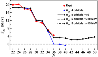
Figure 4: Experimental and theoretical two-neutron separation energies for calcium isotopes from $N=22$ to 50. Data are taken from Audi et al. (2003); Wienholtz et al. (2013); Michimasa et al. (2018). See text for details.

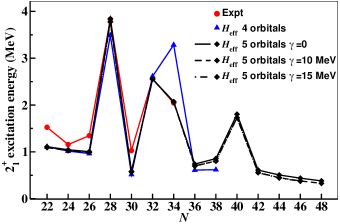
Figure 5: Experimental and theoretical excitation energies of the yrast $J^{\pi}=2^{+}$ states for calcium isotopes from $N=22$ to 50. See text for details.

In Fig. 5 we have also reported the results we obtain by employing the Hamiltonian $H^{\prime}$ in Eq. 3 with values of $\gamma=10$ MeV (dashed black line) and 15 MeV (dash-dotted black line). As can be seen, the center-of-mass spuriosities provide a little contribution also for the calculation of the excitation energies of the yrast $J^{\pi}=2^{+}$.

It is now worth recalling that in the Introduction we mentioned about the role that continuum states may play in isotopic chains approaching their drip lines. In a recent paper we investigated the neutron drip line of oxygen isotopes Ma et al. (2020), which is experimentally placed at $N=24$, by writing the many-body Hamiltonian in the Berggren basis and deriving a $H_{\rm eff}$, built up in terms of the present chiral $NN$ and $NNN$ potentials, that accounts for continuum states. We have observed that this adds an additional repulsive effect to the one provided by the $NNN$ component of the nuclear potential, and leads to a better agreement with experiment too.

A similar procedure might be employed also to study calcium isotopes, but the present limits of our computational resources prevent to derive $H_{\rm eff}$ with the same accuracy we have done within the HO basis, and we are working to implement continuum effects in the future also for $fp$ isotopic chains.

There are two points that should be worth discussing in connection with the outcome of our calculations, namely the effects of many-body correlations and the sensitivity of our results with respect to the position of the neutron $0g_{9/2}$ orbital.

As regards the first one, we have already mentioned in the previous section that we include the effect of second-order three-body diagrams, which, for systems with more than 2 valence nucleons, account for the interaction of the valence nucleons with core excitations as well as with virtual intermediate nucleons scattered above the model space, via the $NN$ potential Ellis and Osnes (1977).

This, as reported in Section II, has been done by deriving a density-dependent two-body contribution at one-loop order from the three-body correlation diagrams, and summing over the partially-filled model-space orbitals, to overcome the limitations of our SM codes. Here, we want to show the difference of the results of SM calculations performed including or not the effects of such three-body correlations.

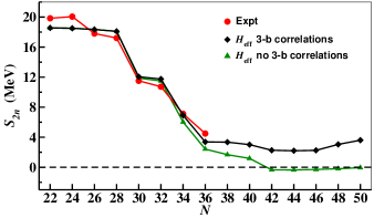
Figure 6: Same as in Fig. 4, but including the results obtained without three-body correlations (green triangles).

To this end, in Figs. 6,7 we compare experimental two-neutron separation energies and excitation energies of yrast $J^{\pi}=2^{+}$ states (red dots), respectively, of calcium isotopes up to $N=50$, with the results of SM calculations obtained including the effect of three-body correlations (black diamonds), which means considering density-dependent $H_{\rm eff}$s, and with those obtained with $H_{\rm eff}$ derived for just the two-valence nucleon system (green triangles).

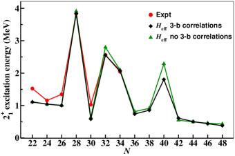
Figure 7: Same as in Fig. 5, but including the results obtained without three-body correlations (green triangles).

As can be seen, the effect of three-body correlations increases with the number of valence nucleons, and starts to be substantial from $N=34$ on. The role of this effect is far more important for the ground-state energies than the calculated excitation energies, and it is extremely relevant to soundly determine the drip line. In fact, without considering many-body correlations we see that the drip line of calcium isotopes is located at $N=40$, while the attractive contribution of second-order correlation diagrams shifts the last bound nucleus at least to ⁷⁰Ca.

The second point that should be examined is the correlation between the SP spacings we have employed for our calculations, as reported in Table 1, and the evolution of the calculated two-neutron separation energies. Our SP spacings have been derived as the energy spectrum of the effective Hamiltonian of one-valence nucleon systems, and they should reproduce the experimental spectra of SP states in ⁴¹Ca (and ⁴¹Sc for protons).

As a matter of fact, the experimental information about the spectroscopic factors of ⁴¹Ca are rather scanty, and in fact the observed counterpart of the second column in Table 1 is missing. However, there are three well-identified SP states in ⁴⁹Ca, whose spectroscopic factors with respect to doubly-closed ⁴⁸Ca have been measured ens ; Uozumi et al. (1994), and they are reported together with the calculated values in Table 3.

Table 3: Experimental negative-parity energy levels (in MeV) of ⁴⁹Ca ens $J^{\pi}=\frac{3}{2}^{-}_{1},\frac{1}{2}^{-}_{1}\frac{5}{2}^{-}_{1,2}$ states, compared with the calculated ones. The values in parenthesis are the one-neutron pickup spectroscopic factors Uozumi et al. (1994).

$J^{\pi}$	Expt.	Calc.
$\frac{3}{2}^{-}$	0.000 (0.84)	0.000 (0.96)
$\frac{1}{2}^{-}$	2.023 (0.91)	1.824 (0.97)
$\frac{5}{2}^{-}$	3.585 (0.11)	3.710 (0.0001)
$\frac{5}{2}^{-}$	3.991 (0.84)	4.191 (0.96)

The comparison between data and theory in Table 3, as well as the correct reproduction of the excitation energy of yrast $J^{\pi}=2^{+}_{1}$ state in ⁴⁸Ca - which is strongly linked to the SP energy spacing $\epsilon_{1p_{3/2}}-\epsilon_{0f_{7/2}}$ -, indicate that the calculated SP spacings of natural-parity $0f1p$ orbitals are reliable. As regards the position of the neutron $0g_{9/2}$ orbital, there is no clear experimental indication if our calculated value is reasonable or not.

We have then calculated the odd-even mass difference around ⁶⁸Ni that, because of the observed shell closure of nickel isotopes at $N=40$, has a strong dependence on the energy gap between the $0g_{9/2}$ and $0f_{5/2}$ orbitals, and whose experimental value is 3.2 MeV Audi et al. (2003). The calculation cannot be performed exactly with our present computational resources Caurier and Martinez-Pinedo (2002); Shimizu et al. (2019), so we truncate the dimension of the eigenvalue problem by decomposing the eigenfunctions in terms of broken pairs, and retaining only the components with generalized seniority $v_{g}\leq 4$, the results changing about $0.5\%$ between $v_{g}=3$ and 4. It turns out that our value is 4.2 MeV, 1 MeV larger than the observed one, and indicating that the SP spacing $\epsilon_{0g_{9/2}}-\epsilon_{0f_{5/2}}$ could be overestimated by the same amount.

On the above grounds, we have investigated the sensitivity of our results to the position of the $0g_{9/2}$ SP state, by raising and lowering its energy by 1 MeV with respect to the calculated value.

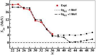
Figure 8: Same as in Fig. 4, but with calculated values are obtained raising (dashed line) and lowering (dotted line) $\epsilon_{0g_{9/2}}$ by 1 MeV.

In Figs. 8 and 9 we report the results obtained with these two new values of $\epsilon_{0g_{9/2}}$ for both the two-neutron separation energies and the excitation energies of yrast $J^{\pi}=2^{+}$, respectively.

We observe that up to $N=40$ the results barely differ each other as well as from those with the set of SP energies in Table 1, and consequently the available experimental values cannot discriminate about the choice of $0g_{9/2}$ SP energy. From $N=40$ a clear distinction is observed: raising $\epsilon_{0g_{9/2}}$ by 1 MeV we obtain that ⁶²Ca is loosely bound with respect to ⁶⁰Ca, and a strong shell closure appears at $N=40$. This shell closure disappears lowering $\epsilon_{0g_{9/2}}$ by 1 MeV, leading to the conclusion that a future measurement of the experimental excitation energy of the yrast $J^{\pi}=2^{+}$ state may provide insight on the location of calcium isotopes drip line.

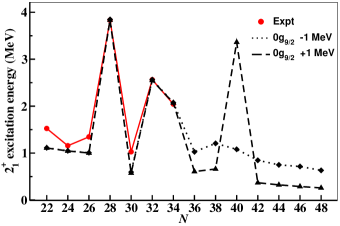
Figure 9: Same as in Fig. 5, but with calculated values are obtained raising (dashed line) and lowering (dotted line) $\epsilon_{0g_{9/2}}$ by 1 MeV.

IV Conclusions

This study is focussed on the location of the neutron drip line of calcium isotopes, as predicted by nuclear shell-model calculations.

It is grounded on the results we have obtained in Ref. Ma et al. (2019), where, starting from two- and three-nucleon potentials derived within the chiral perturbation theory, we have calculated effective SM Hamiltonians able to reproduce the observed closure properties of calcium isotopes and other $0f1p$ isotopic chains. Here, in order to improve the depiction of heavier systems, the model space has been enlarged by adding the neutron $0g_{9/2}$ orbital.

Choosing a larger model space, we have improved the description of the few observables in ^54,56Ca with respect to the results obtained without $0g_{9/2}$ orbital, and have also been able to describe ⁶⁰Ca as a bound system, consistently with a recent experiment Tarasov et al. (2018).

The main outcome of our investigation is, however, the fact that according to our results the calcium isotopic chain is bound up to ⁷⁰Ca, at least, a result that is consistent with the recent Bayesian analysis of different density-functional calculations developed by Neufcourt and coworkers Neufcourt et al. (2019). We have therefore also studied the relationship between our theoretical tools and our prediction of the limits of calcium isotopes as bound systems.

More precisely:

1. we have studied the role played by the inclusion of three-body correlations to calculate binding energies. As a matter of fact, calcium drip line would be placed at $N=40$ by neglecting these attractive contributions.

2. Since the position of the $0g_{9/2}$ single-particle energy is quite relevant when the filling of this orbital starts from $N=40$ on, we have investigated the sensitivity of both the two-neutron separation energies and the behavior of yrast $J^{\pi}=2^{+}$ excitation energy to this shell-model parameter. At present, available data do not allow to verify the reliability of our calculated prediction of $0g_{9/2}$ SP energy, at variance with the $0f1p$ orbitals, and we have found that the location of calcium drip line may be correlated with this quantity. In particular, our calculations indicate that the measurement of the yrast $J^{\pi}=2^{+}$ excitation energy in ⁶⁰Ca could be pivotal to rule out predictions about the last bound calcium isotope.

We consider this last point quite intriguing, since experimental investigations of isotopes heavier than ⁶⁰Ca may be very challenging in a near future, and theory is in charge to point to spectroscopic properties that at the same time should be easier to be measured and provide informations about the “terra incognita” of exotic nuclear systems.

References

- Thoennesen (2013) M. Thoennesen, Rep. Prog. Phys. 76, 056301 (2013).
- Tarasov et al. (2018) O. B. Tarasov, D. S. Ahn, D. Bazin, N. Fukuda, A. Gade, M. Hausmann, N. Inabe, S. Ishikawa, N. Iwasa, K. Kawata, et al., Phys. Rev. Lett. 121, 022501 (2018).
- Meng et al. (2002) J. Meng, H. Toki, J. Y. Zeng, S. Q. Zhang, and S.-G. Zhou, Phys. Rev. C 65, 041302 (2002).
- Hagen et al. (2012) G. Hagen, M. Hjorth-Jensen, G. R. Jansen, R. Machleidt, and T. Papenbrock, Phys. Rev. Lett. 109, 032502 (2012).
- Hergert et al. (2014) H. Hergert, S. K. Bogner, T. D. Morris, S. Binder, A. Calci, J. Langhammer, and R. Roth, Phys. Rev. C 90, 041302 (2014).
- Bhattacharya and Gangopadhyay (2005) M. Bhattacharya and G. Gangopadhyay, Phys. Rev. C 72, 044318 (2005).
- Chen and Piekarewicz (2015) W.-C. Chen and J. Piekarewicz, Physics Letters B 748, 284 (2015).
- Cao et al. (2019) X.-N. Cao, Q. Liu, Z.-M. Niu, and J.-Y. Guo, Phys. Rev. C 99, 024314 (2019).
- Neufcourt et al. (2019) L. Neufcourt, Y. Cao, W. Nazarewicz, E. Olsen, and F. Viens, Phys. Rev. Lett. 122, 062502 (2019).
- Wienholtz et al. (2013) F. Wienholtz, D. Beck, K. Blaum, C. Borgmann, M. Breitenfeldt, R. B. Cakirli, S. George, F. Herfurth, J. Holt, M. Kowalska, et al., Nature (London) 498, 346 (2013).
- Michimasa et al. (2018) S. Michimasa, M. Kobayashi, Y. Kiyokawa, S. Ota, D. S. Ahn, H. Baba, G. P. A. Berg, M. Dozono, N. Fukuda, T. Furuno, et al., Phys. Rev. Lett. 121, 022506 (2018).
- Hagen et al. (2013) G. Hagen, P. Hagen, H.-W. Hammer, and L. Platter, Phys. Rev. Lett. 111, 132501 (2013).
- Efimov (1970) V. Efimov, Physics Letters B 33, 563 (1970).
- Tichai et al. (2018) A. Tichai, P. Arthuis, T. Duguet, H. Hergert, V. Somà, and R. Roth, Physics Letters B 786, 195 (2018).
- Simonis et al. (2017) J. Simonis, S. R. Stroberg, K. Hebeler, J. D. Holt, and A. Schwenk, Phys. Rev. C 96, 014303 (2017).
- Hoppe et al. (2019) J. Hoppe, C. Drischler, K. Hebeler, A. Schwenk, and J. Simonis, Phys. Rev. C 100, 024318 (2019).
- Somà et al. (2020) V. Somà, P. Navrátil, F. Raimondi, C. Barbieri, and T. Duguet, Phys. Rev. C 101, 014318 (2020).
- Ma et al. (2019) Y. Z. Ma, L. Coraggio, L. De Angelis, T. Fukui, A. Gargano, N. Itaco, and F. R. Xu, Phys. Rev. C 100, 034324 (2019).
- Polls et al. (1983) A. Polls, H. Müther, A. Faessler, T. T. S. Kuo, and E. Osnes, Nucl. Phys. A 401, 124 (1983).
- Holt et al. (2012) J. D. Holt, T. Otsuka, A. Schwenk, and T. Suzuki, J. Phys. G 39, 085111 (2012).
- Holt et al. (2014) J. D. Holt, J. Menéndez, J. Simonis, and A. Schwenk, Phys. Rev. C 90, 024312 (2014).
- Bogner et al. (2002) S. Bogner, T. T. S. Kuo, L. Coraggio, A. Covello, and N. Itaco, Phys. Rev. C 65, 051301(R) (2002).
- Entem and Machleidt (2002) D. R. Entem and R. Machleidt, Phys. Rev. C 66, 014002 (2002).
- Machleidt and Entem (2011) R. Machleidt and D. R. Entem, Phys. Rep. 503, 1 (2011).
- Navrátil et al. (2007) P. Navrátil, V. G. Gueorguiev, J. P. Vary, W. E. Ormand, and A. Nogga, Phys. Rev. Lett. 99, 042501 (2007).
- Maris et al. (2013) P. Maris, J. P. Vary, and P. Navrátil, Phys. Rev. C 87, 014327 (2013).
- Fukui et al. (2018) T. Fukui, L. De Angelis, Y. Z. Ma, L. Coraggio, A. Gargano, N. Itaco, and F. R. Xu, Phys. Rev. C 98, 044305 (2018).
- Blomqvist and Molinari (1968) J. Blomqvist and A. Molinari, Nucl. Phys. A 106, 545 (1968).
- Kuo and Osnes (1990) T. T. S. Kuo and E. Osnes, Lecture Notes in Physics, vol. 364 (Springer-Verlag, Berlin, 1990).
- Hjorth-Jensen et al. (1995) M. Hjorth-Jensen, T. T. S. Kuo, and E. Osnes, Phys. Rep. 261, 125 (1995).
- Coraggio et al. (2012) L. Coraggio, A. Covello, A. Gargano, N. Itaco, and T. T. S. Kuo, Ann. Phys. (NY) 327, 2125 (2012).
- Kuo et al. (1971) T. T. S. Kuo, S. Y. Lee, and K. F. Ratcliff, Nucl. Phys. A 176, 65 (1971).
- Suzuki and Lee (1980) K. Suzuki and S. Y. Lee, Prog. Theor. Phys. 64, 2091 (1980).
- Suzuki et al. (2011) K. Suzuki, R. Okamoto, H. Kumagai, and S. Fujii, Phys. Rev. C 83, 024304 (2011).
- Hjorth-Jensen et al. (2017) M. Hjorth-Jensen, M. P. Lombardo, and U. van Kolck, eds., Lecture Notes in Physics, vol. 936 (Springer, Berlin, 2017).
- Caurier et al. (2005) E. Caurier, G. Martínez-Pinedo, F. Nowacki, A. Poves, and A. P. Zuker, Rev. Mod. Phys. 77, 427 (2005).
- Shimizu et al. (2019) N. Shimizu, T. Mizusaki, Y. Utsuno, and Y. Tsunoda, Computer Physics Communications 244, 372 (2019).
- Elliott and Skyrme (1955) J. P. Elliott and T. H. R. Skyrme, Proc. R. Soc. Lond. A 232, 561 (1955).
- Gloeckner and Lawson (1974) D. H. Gloeckner and R. D. Lawson, Phys. Lett. B 53, 313 (1974).
- Liu et al. (2012) L. Liu, T. Otsuka, N. Shimizu, Y. Utsuno, and R. Roth, Phys. Rev. C 86, 014302 (2012).
- Baker and Gammel (1970) G. A. Baker and J. L. Gammel, The Padé Approximant in Theoretical Physics, vol. 71 of Mathematics in Science and Engineering (Academic Press, New York, 1970).
- Hoffmann et al. (1976) H. M. Hoffmann, Y. Starkand, and M. W. Kirson, Nucl. Phys. A 266, 138 (1976).
- Audi et al. (2003) G. Audi, A. H. Wapstra, and C. Thibault, Nucl. Phys. A 729, 337 (2003).
- (44) Data extracted using the NNDC On-line Data Service from the ENSDF database, file revised as of March 15, 2019., URL https://www.nndc.bnl.gov/ensdf.
- (45) See Supplemental Material at [URL will be inserted by publisher] for the list of two-body matrix elements of the shell-model Hamiltonian , derived for 2- and 10-valence nucleon systems.
- Ma et al. (2020) Y. Ma, F. Xu, L. Coraggio, B. Hu, J. Li, T. Fukui, L. D. Angelis, N. Itaco, and A. Gargano, Physics Letters B 802, 135257 (2020).
- Ellis and Osnes (1977) P. J. Ellis and E. Osnes, Rev. Mod. Phys. 49, 777 (1977).
- Uozumi et al. (1994) Y. Uozumi, O. Iwamoto, S. Widodo, A. Nohtomi, T. Sakae, M. Matoba, M. Nakano, T. Maki, and N. Koori, Nucl. Phys. A 576, 123 (1994).
- Caurier and Martinez-Pinedo (2002) E. Caurier and G. Martinez-Pinedo, Nucl. Phys. A 704, 60 (2002).