Optimal non-classical correlations of light with a levitated nano-sphere
Abstract
Nonclassical correlations provide a resource for many applications in quantum technology as well as providing strong evidence that a system is indeed operating in the quantum regime. Optomechanical systems can be arranged to generate quantum entanglement between the mechanics and a mode of travelling light. Here we propose automated optimisation of the production of quantum correlations in such a system, beyond what can be achieved through analytical methods, by applying Bayesian optimisation to the control parameters. Two-mode optomechanical squeezing experiment is simulated using a detailed theoretical model of the system, while the Bayesian optimisation process modifies the controllable parameters in order to maximise the non-classical two-mode squeezing and its detection, independently of the inner workings of the model. The Bayesian optimisation treats the simulations or the experiments as a black box. This we refer to as theory-blind optimisation, and the optimisation process is designed to be unaware of whether it is working with a simulation or the actual experimental setup. We find that in the experimentally relevant thermal regimes, the ability to vary and optimise a broad array of control parameters provides access to large values of two-mode squeezing that would otherwise be difficult or intractable to discover. In particular we observe that modulation of the driving frequency around the resonant sideband, when added to the set of control parameters, produces strong nonclassical correlations greater on average than the maximum achieved by optimising over the remaining parameters. We also observe that our optimisation approach finds parameters that allow significant squeezing in the high temperature regime. This extends the range of experimental setups in which non-classical correlations could be generated beyond the region of high quantum cooperativity.
I Introduction
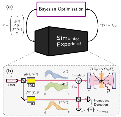
(b) An example of a levitated optomechanics setup. A nanoparticle is suspended via optical tweezers in a harmonic trap. The nanoparticle is then surrounded by cavity mirrors and, by driving the cavity with an external laser, immersed in a cavity field with linewidth . The particle is positioned in the cavity so as to generate a standard optomechanical coupling between the mechanical motion and the cavity field. The pulsed interaction generated by driving on the blue sideband of the cavity resonance frequency generates correlations (two-mode squeezing) between the cavity field and the mechanical motion. The pulse shape and local oscillator profile are controlled by electro-optic modulators (EOM). Optimising over the variables in the external drive provides an enhancement of this effect. The output pulse is detected on a homodyne detector (HD) with the local oscillator modulated as per the temporal profile . The electric signal from the HD is processed and statistically analysed to find the minimal variance of the two-mode squeezing.
Nonclassical correlations are necessary to enhance the performance of a variety of quantum technological tasks, including sensing D. et al. (2018), communications and cryptography N. et al. (2002), quantum computing Deutsch (1985); Jozsa and Linden (2003); Boyer et al. (2017), quantum thermodynamics de Groot and Mazur (1962); Oppenheim et al. (2002); Perarnau-Llobet et al. (2015), as well as having significance for foundational questions in quantum physics Modi et al. (2012). Such correlations have been observed in a variety of physical platforms including optical photons Chen et al. (2014a); Cai et al. (2017); Zhong et al. (2018); Asavanant et al. (2019), cold atoms Madjarov et al. (2020); Gil et al. (2014); Omran et al. (2019), trapped ions Leibfried et al. (2004); Monz et al. (2011); Friis et al. (2018), superconducting circuits Berkley et al. (2003); Steffen et al. (2006), nitrogen-vacancy centres Dolde et al. (2013) and, the platform we address here, optomechanics.
In optomechanical setups, nonclassicality has been observed through the production of squeezed states of mechanical motion in electromechanical systems Wollman et al. (2015); Pirkkalainen et al. (2015), entanglement between distant mechanical systems coupled by light Riedinger et al. (2018) or microwaves Ockeloen-Korppi et al. (2018) and entanglement between the mechanical mode and the microwave mode that leaks from a cavity Palomaki et al. (2013). This is accomplished by engineering a particular interaction between microwaves and mechanics through an external classical driving Hofer et al. (2011). This in turn means that a certain set of experimental conditions must be satisfied in order for the nonclassical correlations to be generated, particularly against the deleterious effects of environmental noise. The determination of these parameters under the constraints of an experimental setting is a complicated optimisation problem even under a small number of tunable variables.
One theoretical method to determine the required parameter values is to develop and analyse a mathematical model of the physical system. Typically, in order to make such a model tractable, many simplifying assumptions must be made. Further, analytical solutions to the problem are often unavailable and the optimisation must proceed numerically. While a broadly applied technique, numerical simulation suffers from a structural weakness, in that the optimisation is guided by the accuracy of the mathematical model rather than the experimental data. Here we invert this viewpoint and propose to use Bayesian methods in optimising the production of nonclassical correlations from an optomechanical system. In our analysis, the optimisation variables are the control parameters that drive the actual experiment and the figure of merit is taken directly from measurements of the system.
Fig. 1 outlines the process. The optimisation proceeds without any preconceived description of the behavioural response of the optomechanical setup to any changes in the control parameters . This is often referred to as treating the setup as a ‘black box’, which in this case produces two-mode squeezing (idealised as , the output of the black box) in response to a set of control parameters . By taking advantage of recent ideas from Bayesian optimisation (BO) Mockus (1989), the results of the black box itself drive the optimisation of the control parameters, not the mathematical model. This in-place optimisation of the experimental parameters we refer to as theory-blind control optimisation.
The theory-blind control idea was pioneered in 1992 under the name ‘learning control’ Judson and Rabitz (1992). Further development and usage has continued, primarily focusing on controlling chemical reactions Phan and Rabitz (1997, 1999); Weinacht et al. (2001); Zhu and Rabitz (2003); Cardoza et al. (2005); Chen et al. (2014b). There are many implementations and ideas using a variety of optimisation algorithms in the quantum information processing (QIP) field. An early example used a hybrid approach, combining classical and theory-blind optimisation, to improve gate fidelities Egger and Wilhelm (2014). This approach was adopted to improve gate fidelities and reduce drift errors in single- and two-qubit gates Kelly et al. (2014, 2016). Further applications of theory-blind optimisation in QIP can be seen in Refs. Dive et al. (2018); Johnson et al. (2017) for example. The theory-blind protocol is advantageously applicable in levitated optomechanics experiments, where a small number of precisely controlled parameters characterise the setup. This can be used to maximise nonclassical correlations and is immediately possible in an experimental setup such as that used in Ref. Delić et al. (2020).
The possibility to achieve two-mode optomechanical squeezing in a specific levitated optomechanical experiment was shown in Ref. Rakhubovsky et al. (2020), and further details of the optomechanical theory used in this manuscript can be found there and in the references therein. Here we take the results of Rakhubovsky et al. (2020) as an initial benchmark and demonstrate that BO is capable of discovering parameter sets that generate significantly stronger two-mode optomechanical squeezing. This is achieved by efficient exploration of the parameter space, particularly in the regimes where analytical description of the optomechanical system is difficult or intractable, specifically, beyond the rotating wave approximation of the resonant-sideband driving, and outside of the resolved sideband. Despite the fact that the generation of nonclassical correlations in optomechanics via a two-mode squeezing interaction is well-investigated theoretically Genes et al. (2008); Hofer et al. (2011); Kiesewetter et al. (2014); Rakhubovsky and Filip (2015); Lin and He (2015); Rudolph et al. (2020); Lin et al. (2020), and has been demonstrated in a number of cryogenic setups Palomaki et al. (2013); Riedinger et al. (2018), it remains a challenging task for new optomechanical platforms such as levitated nanoparticles. Additionally, although some theoretical study has been made into driving correlations through frequencies off the blue sideband Lin and He (2015), only specific fixed frequencies were analysed. Other recent work considers driving off the blue sideband Clarke et al. (2019), but using very short pulses (less than the period of mechanical motion) and in the regime where the optical decay is much greater than frequency of the mechanical oscillator.
Experiments are expensive and time-consuming so in order to show the feasibility of this idea in the specific context of nonclassical states of nano-oscillators, we simulate the protocol. Since the optimisation algorithm does not know that the experiment is simulated rather than real, this functions as a test of the efficacy of theory-blind Bayesian methods to optimise the production of a figure of merit. Mathematical models of optomechanics are particularly robust and well-tested in the linearised regimes that our analysis and simulations focus on herein Aspelmeyer et al. (2014); Bowen and Milburn (2015), thus the process also provides predictions on how to maximise the generation of nonclassical correlations in an optomechanical setting.
The remainder of this manuscript is organized as follows. Section II describes the model used in the simulation of the optomechanical system for calculation of the figure of merit based on the environmental and controllable input parameters. Section III provides an overview of Bayesian optimisation and explains its suitability for this application. Section IV gives results of the simulated theory-blind optimisation procedure, demonstrating how allowing Bayesian optimisation increasing degrees of freedom enables it to discover parameter sets that improve upon the two-mode squeezing levels. The results and their implications are discussed in Section V.
II Theory
In this manuscript we aim at maximising nonclassical optomechanical correlations. This section contains a formal description of the optomechanical system formed by a nanoparticle levitated inside a cavity, and a pulse of travelling light. We provide the Hamiltonian of the optomechanical interaction inside the cavity and obtain the differential equations for the quadratures of the mechanical motion and the intracavity light. With the help of input-output relations we derive a Lyapunov equation for the matrix of covariances between the mechanical motion and the light pulse, and describe how to quantify the nonclassical correlations between them knowing the covariance matrix. This section provides the theory necessary to reproduce our results, more details can be found in Refs. Genes et al. (2009); Rakhubovsky et al. (2019).
II.1 Gaussian Hamiltonian dynamics of opto-mechanical system
Our focus is on a levitated nanoparticle of mass trapped in a tweezer beam within a optical cavity (see Fig. 1 (b)). In this setup, the potential for the mechanical motion of the particle is determined by the spatial intensity profile of the tweezer. The Gaussian profile can be well approximated near the origin by a quadratic potential of a harmonic oscillator parametrized by eigenfrequency . The mechanical motion of the particle is coupled to a cavity mode that itself is a harmonic oscillator characterized by the frequency .
The optomechanical coupling can be introduced in one of two ways depending on the positioning of the nanoparticle inside the cavity and the tweezer polarization. When the nanoparticle is placed in the antinode of the cavity optical mode, its displacement influences the eigenfrequency of the cavity, which induces the so-called dispersive optomechanical coupling Romero-Isart et al. (2011). The dispersive optomechanical coupling is inherently nonlinear in the field quadratures Law (1995); Aspelmeyer et al. (2014). It is, however, typically very weak so in an experiment it is routinely enhanced by a strong coherent driving in the presence of which the interaction is effectively linearized. Alternatively, when the nanoparticle is in the node of the cavity mode, given an appropriate polarization of the tweezer laser, the optomechanical coupling by coherent scattering of the tweezer photons off the nanoparticle into the cavity mode takes place. Such interaction is linear both in the field and mechanical quadratures Gonzalez-Ballestero et al. (2019). It is this type of coupling that allowed ground-state cooling Delić et al. (2020) of levitated nanoparticle. In both cases, the system can be described by the linearized Hamiltonian of the optomechanical interaction Aspelmeyer et al. (2014); Bowen and Milburn (2015)
| (1) |
where are the canonical dimensionless quadratures of the cavity (mechanical) mode normalized such that , and is the time-dependent detuning of the coherent drive (or the tweezer frequency for the coherent-scattering coupling) from the cavity frequency. The coupling strength can be set by the power of the coherent drive (or by power and polarization of the tweezer). In an experiment, the detuning and the drive power (and consequently, ) can be controlled by a suitable modulation (e.g., electro-optical) of the laser light (symbol EOM in Fig. 1 where the case of the dispersive optomechanical coupling is pictured). As we show below, a careful optimisation of these parameters allows achieving stronger optomechanical squeezing compared with the primitive regime of constant-power resonant-sideband driving Rakhubovsky et al. (2020).
In this manuscript we are interested in pulsed driving in the vicinity of the upper mechanical sideband of the cavity at frequency . As is known Genes et al. (2009); Aspelmeyer et al. (2014), driving on the upper mechanical sideband produces an optomechanical interaction which approaches the parametric amplification capable of producing nonclassical correlations by scattering the drive photons to the Stokes sideband. In order to run efficiently, this process requires that the scattering into the anti-Stokes sideband is suppressed, which occurs when the mechanical frequency exceeds the cavity linewidth: .
We assume a pulsed operation, i.e. to be nonzero for and zero otherwise. The advantages of the pulsed manipulation stem from working at shorter timescales compared to the steady states of continuous driving. Since the pulsed operation does not require the system to reach a steady state, it can use coupling strengths that are prohibitively large for the continuous drive. Indeed, driving the optomechanical cavity on the upper mechanical sideband adds into the dynamics of the mechanical mode a negative damping proportional to the driving strength Braginsky et al. (1970). This negative damping easily overwhelms the intrinsic low damping of mechanics thus making its dynamics unstable. In addition, operating at faster timescales helps to decrease the impact of the noisy thermal environment.
The optomechanical system is open, with each of its modes coupled to its corresponding environment. Whereas the optical environment has low noise, the multi-mode mechanical one is at a high temperature. We take this into account in terms of Langevin-Heisenberg equations in the form Rakhubovsky et al. (2020)
| (2) |
where is a vector of unknowns and is a vector of input noises. In this notation, is the cavity linewidth and is the mechanical damping rate. The drift matrix reads
| (3) |
The components of the noise vector satisfy the standard Markovian autocorrelations Giovannetti and Vitali (2001)
| (4) | |||
| (5) |
Here is the Jordan product, is the shot-noise variance, and is the mean occupation of the thermal environment of the nanoparticle. The nanoparticle’s environment manifests itself in a number of ways including collisions with residual gas particles, trapping photon recoil, etc Delić et al. (2020). Therefore, a more experimentally relevant value is the heating rate .
An important characteristic of the input fluctuations is the so-called diffusion matrix defined as , so in our case
| (6) |
II.2 Input-output formalism
Since we are interested in control of the nonclassical correlations between mechanics and the leaking light, that can be directed to another quantum system or detector, we have to obtain an expression for the latter. We start doing so with the input-output relations for a high- cavity Gardiner and Collett (1985)
| (7) |
Next, we define a mode of the leaking light that is detected at the output. This mode is characterized by its temporal profile and is described by quadratures
| (8) |
Because the quadratures satisfy the commutation relation
| (9) |
the mode profile has to satisfy the normalization condition
| (10) |
for to be canonical variables. In an experiment, the choice of different mode profiles , that is detection of quadratures of the modes with different temporal profiles, can be implemented in the homodyne detection by either using a local oscillator with time-dependent amplitude or by frequently sampling the instantaneous value of quadrature with a constant-amplitude local oscillator and subsequently assembling an integral sum of the form Eq. (8) from samples Takase et al. (2019).
The choice of a certain temporal detection profile is a particularly important task in the problem of detecting the quantum correlations Rakhubovsky et al. (2019). A simple intuition can be used in the case when the drift matrix is time-independent. In this case, an analytical solution of the dynamics exists that allows expression of the instantaneous amplitudes of the leaking field in terms of the initial values and the input fluctuations. Such an expression contains a term proportional to with the coefficient . Setting the detection profile equal to this coefficient gives the temporal mode of light that has maximal contribution of . We refer to such a detection profile as the ‘optimal’ profile in Section IV.1.
Having the definitions for the output mode, considering it a function of the upper integration limit, we can extend Eq. 2 to include the output mode
| (11) |
where is the extended vector of unknowns and is the extended vector containing noise terms.
| (12) |
The new drift matrix reads
| (13) |
and for the diffusion matrix we obtain
| (14) |
Above we used notation for an -dimensional identity matrix, and for a matrix of zeros of corresponding dimensions.
The dynamics of the system are linear, therefore the initial multimode zero-mean Gaussian state and multimode zero-mean Gaussian state of the noises are mapped by Eqs. 2 and 11 onto another zero-mean Gaussian state. An important feature of such states is that they are fully described by their second moments that form a covariance matrix. The latter is defined as
| (15) |
The covariance matrix evolution is governed by the matrix Lyapunov equation:
| (16) |
To analyze the nonclassical optomechanical correlations of the modes of our interest, we derive the covariance matrix of a bipartite system formed by the nanoparticle and the leaking light by keeping only the corresponding rows and columns in . In our particular case, we remove the first two rows and columns, and arrive to a covariance matrix with .
II.3 Optomechanical two-mode squeezing
From the covariance matrix of the bipartite optomechanical system we obtain the two-mode squeezing from its minimal eigenvalue . A squeezed state is indicated by , with squeezing increasing as decreases. The two-mode optomechanical squeezing is given by
| (17) |
which is clearly maximised for minimal .
Detection of the two-mode squeezing of a bipartite system does not require full state tomography. A simple method exists that allows this detection via only one homodyne measurement of each of the two modes. The method is based on the fact that in the eigenbasis where the covariance matrix is diagonal, the smallest eigenvalue of the covariance matrix is one of its elements. This means that by a two-mode passive linear transformation it is possible to obtain a generalised quadrature whose variance equals the smallest eigenvalue of the original covariance matrix Simon et al. (1994). This method can exhibit squeezing even when conditional variances do not Filip (2010). The most general of such transformations maps the initial quadratures onto a new set, of which we are interested in the one given by
| (18) |
with being the quadratures of each subsystem in a rotated basis
| (19) |
Equation 18 thus describes an output quadrature of a virtual beamsplitter having an amplitude transmittance with the rotated quadratures of the original modes as the two input modes. The variance of can be computed as
| (20) |
where
| (21) |
and is the rotation matrix:
| (22) |
For an optimal set of angles the corresponding variance assumes the value of the minimal eigenvalue of :
| (23) |
In the lab, one can directly measure using homodyne detection. The phase is set by the local oscillator. The weighting factors can be optimized offline. The problem of detecting the two-mode squeezing is then reduced from the full Gaussian tomography of the bipartite state to the direct homodyne detection of a pair of quadratures Rakhubovsky et al. (2020).
Note that we simplify the problem of evaluation of the two-mode squeezing by assuming that we have an access directly to the mechanical part of the covariance matrix. Though technically such a direct access is impossible, the mechanical quadratures can be effectively swapped to a subsequent pulse of leaking light by driving the optomechanical cavity on the lower mechanical sideband . The state swap procedure via a red-detuned drive is known to be equivalent to an almost noiseless beamsplitter-like transformation from mechanics to the light Vanner et al. (2015); Rakhubovsky and Filip (2017). The problem of the optimal pulse shape is not relevant to the task of state swap as it is for the generation of squeezing. Therefore, an extension of the problem to include the verification step would only be a technical addition to the problem and would not necessarily extend the scope of the manuscript. Thereby, we analyse here an optimized upper bound on directly detectable squeezing from the experimental setup with the key time-variable parameters and .
III Bayesian optimisation
With the elements of theory developed in the previous section, both the task of creating and detecting squeezed states in optomechanical systems can be turned into an optimisation problem. As ultimately these optimisations should be performed directly onto an experimental apparatus, it is desirable that the optimisation routine should converge in a small number of steps, and exhibit robustness with regards to experimental noise. Since Bayesian optimisation (BO) has been successful with these requirements, with examples in quantum optimal control problems Wigley et al. (2016); Zhu et al. (2018); Henson et al. (2018); Nakamura et al. (2019); Mukherjee et al. (2020); Sauvage and Mintert (2019), it is deemed appropriate for the tasks at hand.
A typical optimization problem involves maximising a figure of merit with respect to control parameters ,
| (24) |
In general, can be an -dimensional vector where is the total number of parameters. In our case, it can describe the control parameters and entering the Hamiltonian in Eq. (1), the pulse duration , the detection output profile appearing in Eq. 8 or the detection angles in Eq. (18). On the other hand the figure of merit to be maximised can be the two-mode squeezing value in Eq. (17) or, equivalently, the minimum eigenvalue of the covariance of the optomechanical state described by the matrix .
This search for optimal control parameters is performed iteratively. At each iteration of the algorithm the figure of merit is evaluated for a given set of parameters, from either numerical simulation or experimental data, this information is passed to the optimisation routine, which in turn suggests a new set of parameters to be tried.
In contrast to other optimisation routines, BO relies on the construction of an internal approximation (model) of the relationship between the control parameters and the figure of merit . This model then guides the optimisation process. The choice of the next set of control parameters is turned into a Bayesian decision problem, incorporating an incentive to explore the parameter space. These two steps, of updating the model based on the full set of evaluations collected and choosing the next set of parameters, form a single iteration of BO, and are briefly explained in the rest of this section. More thorough descriptions of BO can be found in Refs. Brochu et al. (2010); Snoek et al. (2012); Frazier (2018); Shahriari et al. (2015).
As based on a limited number of evaluations, which are potentially non-exact due to experimental noise as a source of variance, such as infidelity in applying the controls, it is convenient to adopt a probabilistic modelling approach, that is random functions are used to model the unknown . The prior distribution over these random functions is chosen such that it favours well-defined and regular functions. In more technical terms it means that is taken to be a Gaussian process Williams and Rasmussen (2006). A single evaluation of the figure of merit for control parameters is denoted which is allowed to deviate from the true value due to potential noise in the acquisition of the data. Then, given a record of evaluations of the figure of merit denoted as a vector , one aims at updating the prior distribution to take into account the data collected. This is done by means of Bayes’ rule
| (25) |
where the term denotes the likelihood of obtaining the data-set for a given function and acts as a normalisation constant. When the noise in the data is assumed to be normally distributed, and with constant strength, this conditional distribution can be obtained in closed-form Williams and Rasmussen (2006).
Rather than a single point estimate , this modelling approach allows to obtain the full probability distribution which can be used to select the next set of parameters to be evaluated. One could choose for which the value of is maximal in average. However, as the internal BO model is based only on a restricted amount of data it is likely that this average value may deviate significantly from the true value of especially far away from the parameters already evaluated. Thus it is vital to also explore other promising regions of the parameter space. These considerations can be formulated in terms of an acquisition function, which grades a set of pseudo randomly generated potential parameters, and the choice of the next parameters is taken where this acquisition function is maximised Brochu et al. (2010).
The Expected Improvement (EI) acquisition function is the type predominantly used to generate the results presented in Section IV, defined as
| (26) |
where is the best evaluation recorded so far. That is, the evaluation of that returned the highest figure of merit value. It effectively quantifies the expected improvement compared with the best recorded output from previous iterations, specifically in our case that is the increase in two-mode squeezing level, and encourages exploration where the width of the distribution is large. For the interested reader, a more detailed explanation of how this EI acquisition function achieves this can be found in Ref. Brochu et al. (2010). This exploration feature ensures that a global search is performed making BO less prone to be trapped in local minima.
IV Optimisation results
IV.1 Constant coupling strength
Previous (analytical, without optimisation) work has investigated what can be achieved in terms of two-mode squeezing with a square-shaped driving pulse Rakhubovsky et al. (2019, 2020). The optimisation objective is to maximise the figure of merit, which is the two-mode generalised squeezing , with the optimal values of coupling strength and duration to be determined. Here we consider only these two parameters, which describe a square-shaped (top-hat) pulse, for optimisation to allow comparison with the previous work, which requires using the model with the least number of parameters possible as optimisation variables. We use the analytically derived optimal profile for the measurement function described in Section II.2. is calculated through simulation of the model described in Section II. Technical details of the simulation are given in Appendix B, which also gives detailed descriptions of the optimisation methods. The simulation is broadly based on the experimental setup used in Ref. Delić et al. (2020). The system parameters are summarised in Table 1.
The pulse parameters and are constrained with experimentally relevant upper bounds of and respectively, where is the optical damping. Moreover, some combinations of pulse parameter values would lead to overheating, potentially damaging the system, and so a further constraint is applied using an adiabatic approximation of amplitude gain given by Eq. 42.
The interactions with the environment are modelled as described in Section II. The bath temperature is characterised by the mean number of bath phonons . Combined with the mechanical damping this gives rise to a reheating rate . The temperature of the oscillator is characterised by the mean mechanical occupation . The model does not predict that cooling of the oscillator significantly increases the potential two-mode squeezing level , except for extremely low temperatures (). Therefore, for now, the oscillator is considered to be initially (prior to the driving pulse) in thermal equilibrium with the bath, that is . Later, in Subsection IV.4, we will see that cooling the oscillator is beneficial in terms of resilience to measurement imprecision.
The maximum achievable two-mode squeezing is dependent on the reheating rate Rakhubovsky et al. (2019). This is illustrated in Fig. 2, which presents the squeezing level (in dB) level achieved by optimising and for specific bath temperatures over a wide range. The relationship of to is also plotted for three fixed combinations, with the amplitude at maximum in each case. The required pulse parameters to achieve this maximum squeezing also vary with the reheating rate. The optimal values for and for the different values of were found using Bayesian optimisation (BO).
At lower temperatures the squeezing process is adiabatic and a long pulse is most effective, whereas at higher temperatures greater coupling is required to achieve maximal . Reheating rates where the squeezing process is adiabatically driven are not achievable in the lab Delić et al. (2020); Sommer et al. (2020). Current experimental setups can achieve reheating rates as low Delić et al. (2020), which is in the region where gradient of with respect to is at its steepest. This is also the region where the squeezing level is most sensitive to pulse parameter values and . This relationship is further examined in Section B.3.
Measurable squeezing is still predicted at higher reheating rates. For a high bath temperature characterised by phonon number , with corresponding reheating rate , we find that squeezing is possible through driving with a top-hat shaped pulse. With the driving pulse constraints used here, the generalised squeezing becomes effectively immeasurable () at some reheating rate limit . The squeezing levels plateau in this thermal region, and only actually reach zero for reheating rate . The upper reheating rate limit of measurable squeezing could potentially be raised if the amplitude gain limit (fixed at in throughout this study) could be safely set higher. Note that this plateauing is related to the mechanical frequency , which is further illustrated and explained in Section B.4.
In the experimentally relevant heating range the pulse parameter values need to be chosen carefully in order to maximise two-mode squeezing for the particular thermal parameters, which are likely to fluctuate and may be difficult to estimate precisely. If the environmental parameters in an experiment attempting to drive and measure two-mode squeezing differ from the ones used to theoretically determine the pulse parameters, maximum possible squeezing will not be achieved. Theory-blind optimisation will determine the correct pulse parameter values to reach maximal two-mode squeezing levels.
Despite these positive results, the top-hat shape is not necessarily optimal for the coupling pulse profile. The next section investigates the potential for improving on maximum squeezing by allowing for a temporally shaped pulse.
IV.2 Time-dependent coupling
The signal generators used in state-of-the-art optomechanics experiments allow for effectively any continuous time-dependent function to be applied to temporally shape the laser pulse amplitude driving the coupling. That is, with pulse durations on the order of those used here, it is valid to consider an arbitrarily shaped coupling function . Hence the search space for the optimisation can be expanded by adding variables that will allow for a time-dependent shaped coupling. The measurement function used for a top-hat shaped driving pulse, cannot be assumed optimal for an arbitrary shaped pulse, and so any optimisation of parameters for the driving pulse must be combined with optimisation of parameters for the measurement function . In a physical experiment such as in Fig. 1 these functions are controlled by modulators (EOM).
With time-dependent coupling it is necessary to calculate the covariance matrix by numerically solving Eq. (16). The technical details of how this is performed, including the pulse parameterisation scheme, are given in Appendix B.1. The rotating wave approximation (RWA) gives rise to some differences in for some top-hat pulse parameters when the mechanical frequency is in the order of the optical damping, and so the analytical solution to differs from the numerical solution with the mechanical frequency used here. The numerical solving method is therefore also used here for computing the covariance matrix with the top-hat pulse to ensure a fair comparison.
For the comparison of different optimisation variable combinations the reheating rate is fixed at the experimentally achievable value by setting specific values for the environmental parameters . Bayesian optimisation (BO) is again used to determine optimal parameters. In the time-dependent case the piecewise linear (PWL) parameters for the functions and are the optimisation variables, along with the total pulse duration , which is the same for both functions.
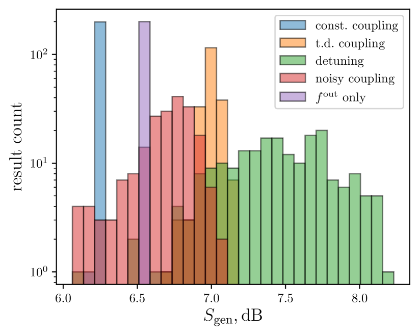
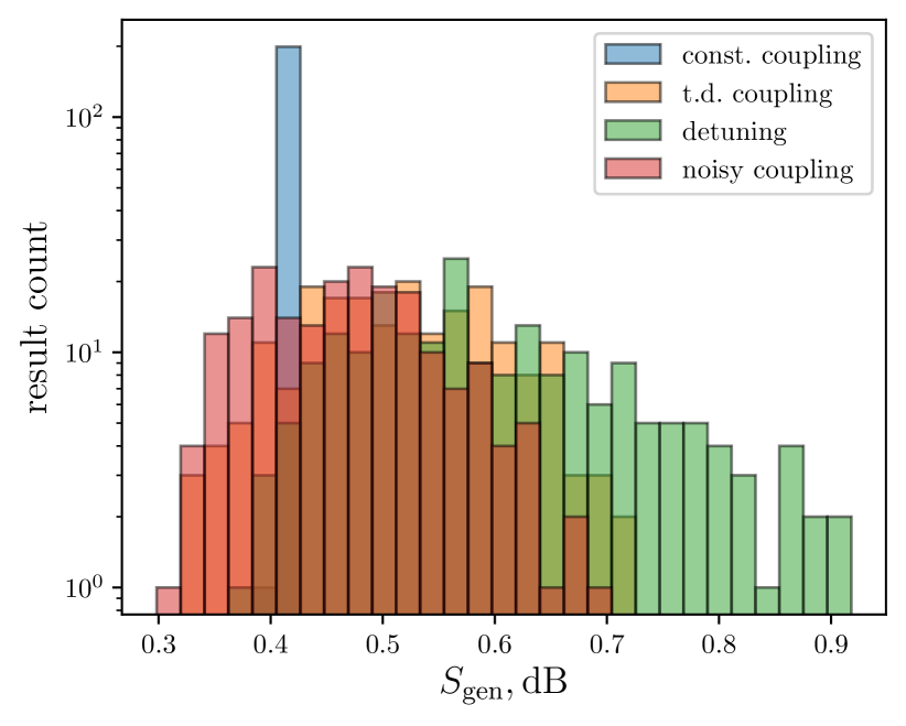
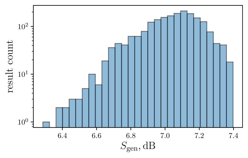
The optimisation results comparing the constant and time-dependent coupling are shown in Fig. 3. There is some variation in the value of found by BO, and so the results of 200 repeats of BO are shown in a histogram. The data from the different optimisation variable combinations are compared on the same axes. The results for the top-hat and time-dependent coupling pulses are labelled ‘const. coupling’ and ‘t.d. coupling’ respectively. In all repetitions the time-dependent pulses out-perform the top-hat pulses. The minimum, mean and maximum squeezing are for top-hat and for the PWL pulses, demonstrating that in simulation greater squeezing can be achieved with a temporally shaped coupling strength amplitude.
We find similar upper limit to the reheating rate () for measurable squeezing as for the top-hat pulse, suggesting that the upper bath heat limit cannot be extended through temporal shaping of the coupling strength. However, we do find that at higher reheating rates that optimised PWL shaping increases the level of squeezing beyond what can be achieved with a top-hat pulse. For example, with reheating rate , we find that the PWL parameterisation of the coupling pulse allows squeezing with mean (maximum) , which is an improvement on the achievable with the top-hat pulse.
The distribution of results in terms of maximum achieved squeezing is understood to be caused by local maxima (traps) in the optimisation variable landscape. Local maxima are observed in data for the 2-d constant coupling case when solving the dynamics numerically (without the RWA) that are not seen when the RWA is made. Further explanation of this is given in Section B.3, which includes an illustration of how the RWA affects the squeezing computation and plots of the optimal pulses from this subsection.
IV.3 Detuning frequencies
The results presented so far have been obtained for a fixed driving laser frequency detuning . Solving the dynamics numerically also allows for the detuning to be offered as a variable for optimisation. Giving a single additional degree of freedom to Bayesian optimisation (BO), that is a fixed value for the detuning throughout the driving pulse, provides little improvement in the maximum achievable squeezing. However, allowing a time-dependent profile for the detuning, by optimising the parameters of a piecewise linear function , enables significantly greater two-mode squeezing.
The results for repeated optimisations maximising including the detuning variables can be seen in Fig. 3. The results for all the optimisation variable combinations are compared on the same axes. The distribution of 200 repetitions of the optimisation of , , is labelled ‘detuning’. The duration of the pulse is also an optimisation variable. There is a greater spread in the results than when optimising just and , but the mean final squeezing () is greater than the maximum () achieved without optimising the detuning, and the maximum achieved with optimised detuning is .
Again we find the upper limit to the reheating rate () for measurable squeezing as for the top-hat and PWL pulses with fixed detuning frequency, suggesting that the upper bath heat limit cannot be extended through temporally shaping the detuning. However, we do find that temporal shaping of the detuning also increases squeezing at higher reheating rates. For the high bath temperature, with reheating rate , we find that the detuning frequency modulation allows squeezing with mean (maximum) , which is a further improvement on the found for optimised PWL coupling strength fixed detuning frequency. Illustration of this comparison given in Section B.4. We emphasise that all types of pulse are bound by a limit on the amplitude gain (given by Eq. 42), and so this comparison is made at the physical (overheating) limit of the optomechanical system.
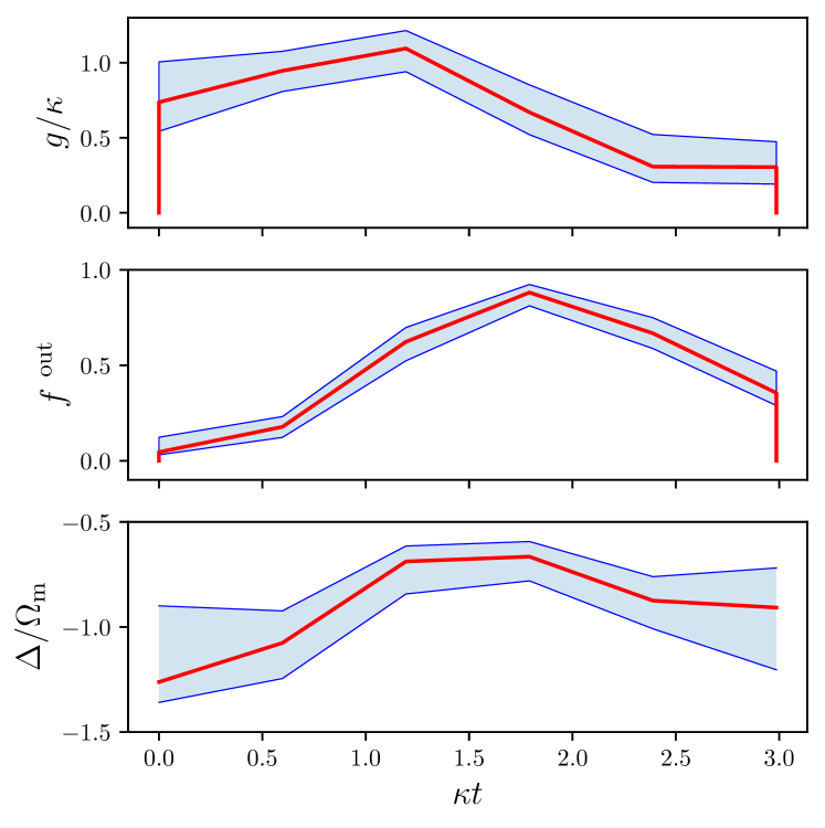
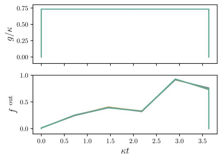
Fig. 4 shows the time-dependent profiles of the optimal , and . The plots give a representation of the average pulse (see figure caption for definition). There is actually a wide variety of pulse profiles that produce high squeezing, which is explained in Section B.3. The average pulses give an indication of common features. For the driving pulse we see a stronger coupling initially, with a peak before the middle, then tailing off towards the end. For the measurement function we see this starts around zero, increasing up to a peak after the middle, and then tailing off partially. The detuning functions have much greater variation, but typically start below the blue sideband , rising to above in the middle, and finishing around .
The particular result for the detuning temporal profile is interesting, as most analytical studies have assumed fixed detuning at the blue sideband for driving two-mode squeezing. Possibly, the time-dependent detuning helps counteracting the noise, and hence leads to greater squeezing. Some evidence for this is observed when setting the mechanical oscillator frequency much greater than the optical damping (). The optimised time-dependent profile for the detuning is then at the blue sideband when the coupling is at its strongest.
IV.4 Detection angles
In an experimental setting, estimating would require full state tomography. There is a potentially more efficient method of measuring , described in Section II.3, based on the equivalence of to . This method requires three parameters to be determined: . The latter is a weighting that can be determined in post processing. The homodyne measurement angles are experimental settings that could be determined through theory-blind optimisation. To test this idea in simulation, in which the full covariance matrix is computed by numerically solving Eq. (16), is calculated as per Eq. (20). The optimisation algorithm is given only as variables, and the figure of merit is calculated from a fixed . In an experiment this is equivalent to running with identical driving parameters.
For covariance matrices computed numerically, without the rotating wave approximation, with the experimentally achievable reheating rate and the mechanical oscillator initially in thermal equilibrium with the bath, optimisation algorithms are unable to navigate the parameter landscape to reliably find the equivalent to , as the minima is located in a narrow trough. This is explained further in Appendix B.5. This would be further compounded in an experimental setting, as the measurements would be intrinsically noisy.
When the initial temperature of the mechanical oscillator is much lower than the environment temperature , for computed through simulations, the upper bound of is much lower, which also reduces the sharp changes in gradient. The optimisation algorithm is able to reliably find equivalent to , so long as the oscillator is sufficiently cooled, for example phonon number . Much lower values than this are now achievable in experiment Delić et al. (2020). Therefore this method for estimating the two-mode squeezing by determining homodyne measurement angles through theory-blind optimisation remains a viable option. Note that this only helps the measurement process, and that the squeezing is only significantly increased for much lower oscillator temperatures of .
IV.5 Control noise
In an experimental setting the precision to which controls can be applied will be limited. Also, how the system will respond to the controls may not be fully predictable. In this specific example of controlling the coupling of the oscillator to the light field by modulating the amplitude of the laser, it is likely that the actual coupling may have some random variation in its response. This is referred to as control noise. The optimisation algorithm is guided by the outcome of trying specific sets of parameters. Variation in the outcome will lead to reduced performance of the algorithm. One method to overcome this would be to repeat the experiment with the same parameters multiple times and take the mean outcome, however this would greatly increase the total number of times the experiment would need to be run. Bayesian optimisation (BO) can refine its model of the control landscape, taking into account that the figure of merit function value for some set of parameters may not be exact.
To replicate this scenario that one would encounter in the lab and to verify the stability of optimisation the control noise is modelled by adding some pseudo-random Gaussian distributed value to the pulse parameters. Further details are given in Appendix B.6. The results for BO maximising by optimising and when noise (standard deviation of amplitude) is added to the piecewise linear parameters of are shown in Fig. 3. These results are compared with others on the same axes, the distribution of squeezing achieved with 200 repeats of BO with noisy coupling parameters is labelled ‘noisy coupling’. These can be compared with the distribution when and are optimised without control noise (labelled ‘t.d. coupling’), as the detuning is fixed at the blue sideband in both cases. Although there is greater spread in the distribution, with minimum, mean, maximum being for the noisy controls, compared with in the noiseless case, BO still performs very well.
V Summary and Outlook
We have optimised the production of nonclassical optomechanical correlations, as measured by the two-mode squeezing . This is accomplished by adding a layer of Bayesian optimisation to the control variables, such as coupling rate , pulsed interaction duration , drive detuning and the detection profile , so that repeated simulations of the optomechanics experiment are directed towards increased nonclassical correlations. Such control variables must be optimised against the uncontrolled parameters such as the heating rate that negatively affect the production of nonclassical correlations. The optimisation shows that this can be accomplished in a way not easily replicable by analytical studies of the mathematical model.
For example, in the case of a pulse of constant interaction strength the optimisation distinguishes between various reheating regimes and pulse lengths in order to maximise the optomechanical squeezing , thus granting access to higher two-mode squeezing in experimentally relevant regions of the reheating variable. Adding more variables to the optimisation procedure, including time-dependent couplings and measurement functions , only adds to the power of the optimisation procedure. While requiring more resources to optimise, plainly having a greater parameter landscape to explore provides more opportunity to increase the optomechanical squeezing. We have assumed a certain fixed complexity of this time-dependence in the form of piece-wise linear functions, however it seems reasonable to conjecture that increasing the detail of such functions, and therefore the number of control variables, will produce more finely tuned optimisations with greater nonclassical correlations.
Curiously, the optimal coupling profile , measurement function and detuning profile must be used as a set, in the sense that taking an average of the optimised functions does not produce high levels of squeezing (when compared with the maximum achieved). We find that detuning away from the blue-sideband, in combination with the other optimised variables, produces noticeably greater squeezing than otherwise predicted Rakhubovsky et al. (2020). The blue detuned drive produces nonclassical correlations perfectly in a unitary system, and we deviate from this by including noise effects from the thermal environment. Allowing the control variables to vary around this unitary ideal gives the optimisation an opportunity to locate the deviated maximum squeezing. For an estimate, while the non-optimized case predicts generation of approximately dB of the optomechanical squeezing for the heating rate , after the optimisation over all experimentally controllable parameters () the squeezing can reach values over dB.
The optimisation not only increases the magnitude of the optomechanical squeezing but, compared to the non-optimized case Rakhubovsky et al. (2020), allows to achieve squeezing in the case of significantly higher temperatures of the environment. We have not specifically addressed the problem of finding the maximal heating rate allowing generation of the optomechanical squeezing, because the solution of such a problem is a set of optimal parameters that yields squeezing approaching zero at a high temperature. On the contrary, we have focused on the maximisation of squeezing at a fixed, experimentally reasonable, value of the temperature of the environment corresponding to a certain value of . For instance, at the high temperature of the mechanical environment that corresponds to the heating rate , driving the system with a top-hat pulse yields dB of squeezing. The pulse with all the parameters () optimised can exhibit detectable squeezing as high as dB at this value of the heating rate. Note that from the point of view of the quantum cooperativity Aspelmeyer et al. (2014), which compares the optomechanical coupling rate with the decoherence rates of the system , at this high temperature, our system is clearly outside the regime of high cooperativity.
While we have emphasised experimental values from a certain levitated setup Delić et al. (2020) in the text, the present simulations can be applied to other levitated experiments Monteiro et al. (2013); Hempston et al. (2017); Pontin et al. (2018); Meyer et al. (2019). Moreover, any optomechanical Meenehan et al. (2014); Nielsen et al. (2017); Shomroni et al. (2019) or electromechanical Barzanjeh et al. (2019); Peterson et al. (2019) system capable of functioning in the pulsed regime of linearized optomechanical interaction can be analysed using exactly the same tools. The latter also allow consideration of multiple mechanical oscillators for investigation of mechanical-mechanical correlations generated by the pulsed interaction. Furthermore, the problem can be extended to include two- and three-dimensional motion of the levitated nanoparticles, which allows consideration of non-classical correlations between the motion of one or multiple nanoparticles in orthogonal directions van Loock and Furusawa (2003); Chang et al. (2020).
The theory-blind process can be interfaced directly with an experimental setup, in which one can imagine an autonomous process that repeatedly inputs new control variables in response to a Bayesian update from the optimisation, producing large values of squeezing. Bayesian optimisation improved upon the theoretically predicted optimal parameters for driving two-mode squeezing in the numerical model. The efficient method for measuring the squeezing by determining the optimal homodyne measurement angles through optimisation has also been demonstrated viable through simulation. The theory-blind optimisation process in this application has therefore been thoroughly tested in simulation and demonstrated to be valuable. The technological requirements for shaping the frequency and amplitude of the driving pulses, and the coordinated measurement of the output, all controlled by some automated process, are available in most labs experimenting with optomechanical setups. A parameter set found to be optimal in simulation is unlikely to be the optimal solution in the lab, due unexpected couplings, parameter drift, and other sources of noise. Theory-blind optimisation would find the true optimal solution for the specific set, in the specific moment, as this is based on response and measurements from the actual system. Further improvement upon the maximum two-mode squeezing level found in simulation could potentially be achieved through this full theory-blind optimisation, for instance taking advantage of attributes of the setup that were not modelled in the simulation, such as nonlinearities in the coupling Sankey et al. (2010); Leijssen et al. (2017) and non-Markovianity Gröblacher et al. (2015) in the environmental interactions.
VI Acknowledgements
The project Theory-Blind Quantum Control TheBlinQC has received funding from
the QuantERA ERA-NET Cofund in Quantum Technologies implemented
within the European Union’s Horizon 2020 Programme and from EPSRC under the grant EP/R044082/1.
The Supercomputing Wales clusters were used run the many simulations behind the results.
We are grateful for the free access to this resource.
A.A.R, D.M. and R.F. were supported by the Czech Scientific Foundation (project 20-16577S), the MEYS of
the Czech Republic (grant agreement No 731473), the Czech Ministry of
Education (project LTC17086 of INTER-EXCELLENCE
program) and have received national funding from the
MEYS and the funding from European Union’s Horizon 2020 (2014-2020) research and innovation framework
programme under grant agreement No. 731473 (project 8C18003 TheBlinQC).
F.S. was supported through a studentship in the Quantum Systems Engineering Skills and Training Hub at Imperial College London funded by EPSRC(EP/P510257/1).
A.R., D.M., and R.F. acknowledge discussions with M. Aspelmeyer, N. Kiesel and U. Delić.
Appendix A Approximations in the theory of cavity optomechanics
A.1 Dynamics of slow opto-mechanical amplitudes
To investigate the interaction between the optical and mechanical modes, it is instructive to switch to the rotating frame defined by the free evolution of the modes (the first two terms in Eq. 1). This is equivalent to a transition from the instantaneous values of the quadratures to their slowly varying envelopes following the rule
| (27) |
with , where is the matrix of unitary rotation
| (28) |
Substituting Eq. 27 into Eq. 2 yields the equations of motion for the envelopes :
| (29) |
completely analogous to Eq. 2 with notations
| (30) |
In particular, the full expression for reads
| (31) |
with notation
| (32) | |||
| (33) |
Also for the noises one can write
| (34) |
A Lyapunov equation with the matrices substituted according to the rule can be written for the equations of motion Eq. 29. It is important to note that this equation is exact and valid for an arbitrary detuning.
A.2 Rotating wave approximation
To simplify the further analysis, we assume that the system is operated in the resolved-sideband regime, where the mechanical frequency significantly exceeds the linewidth of the cavity, and the opto-mechanical coupling is weak: , that the drive tone is tuned to the upper (blue) mechanical sideband of the cavity: , where . After substitution of the detuning we apply the rotating wave approximation (RWA) which amounts to ignoring all the rapidly oscillating terms in the equation of motion Eq. (29). As a result, the equations are greatly simplified. In particular, we immediately see that the matrices and vanish as they are comprised of rapid terms only. In the interesting case of driving exactly on resonance (),
| (35) |
so the drift and diffusion matrices take the simple time-independent form
| (36) |
These matrices can as well be used to compute a covariance matrix using a Lyapunov equation analogous to Eq. 16.
Importantly, since the coefficients in the equations of motion in RWA are time-independent, these equations can be solved analytically:
| (37) |
One can then proceed substituting this solution into the definition of the covariance matrix to compute the latter.
In the particular case of RWA an analytical solution for the quadratures can be obtained by substituting solution Eq. (37) into the input-output relations Eq. (7) and the definition of the pulse quadratures Eq. (8). Substitution of this solution into definition of the covariance matrix yields an analytical expression for . If, in addition to the condition of resolved sideband, the condition of weak coupling and long pulses is satisfied, the intracavity optical mode can be adiabatically eliminated and the dynamics of the quadratures approaches the pure two-mode squeezing described by the transformations Hofer et al. (2011)
| (38) | ||||
| (39) | ||||
| (40) | ||||
| (41) |
Here we define the amplification gain and the measurement weight function which in the adiabatic regime have simple expressions:
| (42) |
The quantities and are the canonical quadratures of the input light defined in an analogy with Eq. 8 with the mode profile .
Appendix B Simulation and optimisation methods
B.1 Simulation of the optomechanics
The model for the optomechanical system under study is described in Section II. The objective throughout this manuscript is to maximise two-mode squeezing, which is calculated from the covariance matrix using Eq. (17). The system model is characterised by the parameters that are summarised in Table 1. Given these parameters, an analytical solution for the covariance matrix, for a constant coupling pulse applied for a duration , was derived for the study reported in Ref. Rakhubovsky et al. (2019). An implementation of this developed in Python is used in this study, utilising functions from the NumpPy library. The calculation includes the rotating wave approximation (RWA) described in Appendix A.2. In all cases where is computed for a constant (or square) pulse, then the measurement function used is that referred to as ‘optimal’ in Ref. Rakhubovsky et al. (2019). A variation of this code, developed for the study, that gives an exact solution for using the RWA, where and are piecewise constant functions in three timeslots, was used to validate the numerical solutions for .
| sym | desc | default | min | max |
|---|---|---|---|---|
| optical damping | 1 | n/a | n/a | |
| mechanical damping | n/a | n/a | ||
| coupling | 0.1 | 0.01 | 2.0 | |
| pulse duration | 30 | 1 | 100 | |
| initial bath phonons | 1 | |||
| initial mech. phonons | 1 | |||
| reheating rate | ||||
| amplitude gain | n/a | n/a | 50 | |
| mechanical frequency | n/a | n/a | 2 | |
| frequency detuning |
For arbitrary time-dependent functions the covariance matrix is computed by numerically solving Eq. (16), which does not require the RWA. The initial value problem solver in SciPy (scipy.integrate.solve_ivp) is used to solve the differential equation. The absolute and relative tolerance need to be set much lower than the default for sufficiently accurate computation (atol=1e-20; rtol=1e-10), as very small differences in the smallest eigenvalue have a significant effect on the squeezing. Where any direct comparisons are made between the square and time-dependent coupling pulse are made, the numerical solver is used in both cases, as the RWA does induce significant differences in for mechanical oscillator frequencies in the order of the optical damping () with some values of (see Fig. 5).
It is beneficial for the optimisation algorithm to describe the time dependence using fewer parameters. A piecewise linear (PWL) parameterisation is used for the time-dependent function results in this work. The PWL functions vary only linearly between some specific points within the duration , and at these points the gradient may change, but the function remains continuous. Therefore the time-dependent function can then be described over a number of timeslots by values at the start of the timeslot (and end for the final timeslot). That is, for some PWL function , with . All results reported in this manuscript with time-dependent use PWL parameterisation: with all timeslots of equal duration. All time-dependent profiles in any one computation of have the same total duration .
B.2 Optimisation of parameters
| variables | ||||
|---|---|---|---|---|
| 2 | 40 | 40 | 20 | |
| 13 | 200 | 200 | 80 | |
| 6 | 120 | 120 | 50 | |
| 19 | 300 | 300 | 100 |
In Section IV many results are reported where numerical optimisation is used to maximise generalised squeezing , which is calculated from the simulation of the optomechanical system as described in Appendix B.1. Primarily, a Bayesian optimisation algorithm is used (described in Section III). The variables made available to the algorithm are explained in each of subsections of Section IV. These variables, along with the otherwise fixed parameter values from Table 1, are used to calculate the covariance matrix . The objective of the algorithm is to minimise the minimum eigenvalue of the matrix , which maximises (see Eq. (17).)
As described in Section III, BO generates and updates a model of the objective function on the multi-dimension parameter space, which is often referred to as the surrogate model. The model is initially constructed by taking pseudo-random variable sets in the parameter space. BO then uses an acquisition function to determine the variable sets used to update the surrogate model in iterative steps, guided by evaluations of the objective function. The acquisition function also uses some psuedo-randomness in its selection of variable sets to test. The likelihood of choosing points at a greater distance from near previously found minima, searching for potential minima outside of the already explored regions, can be controlled by choice of acquisition function type and some weighting parameter. Thus the full BO process can be broken down into phases. For this work three phases were used, referred to as ‘initial random’, ‘exploration’ and ‘exploitation’. The number of objective functions evaluations allowed for each phase are denoted , and in Table 2. The exploration phase uses the expected improvement (EI) type acquisition, which gives greater weighing to searching of unexplored regions. The exploitation phase uses the lower confidence bound (LCB) type of acquisition, with weighting such that the searching is mainly constrained to within the region near the current global minima of the surrogate model. That is, the exploitation phase refines the result of the exploration phase.
The specific implementation of a Bayesian optimisation algorithm used in this study is in GPyOpt Authors (2016). A gradient-based algorithm is also used for comparison, and also for computational efficiency in Section IV.4. This is the L-BFGS-B implementation in SciPy Byrd et al. (1995). The GNU Parallel library Tange (2011) is used to efficiently run the many repeated optimisations performed on the high-performance computing clusters.
The excessive amplitude gain that would lead to overheating in an experiment manifests itself as ‘float value overflow’ in simulations when calculating the covariance matrix . Hence cannot be computed for all and within the region defined by the bounds given in Table 1. Therefore, the pulse parameters are further constrained using an adiabatic approximation of amplitude gain given by Eq. 42. The same gain limit constraint is used for all optimisations. The constraint is enforced by choosing as optimisation variables, with the amplitude gain proportion defined as . From these the pulse duration for an optimisation step can be calculated as
| (43) |
The optimisation algorithm explores the parameter space, proposing values for and within the specified bounds, with calculated as per Eq. (43). A variant of this is used when is time dependent during the pulse.
The driving laser frequency detuning enters the Lyapunov equation Eq. (16) in elements of the drift matrix . Consequently, when solving numerically, this can have an arbitrary time-dependent form. Where the detuning is optimised for maximising (Section IV.3), the PWL parameters of a detuning offset function are optimisation variables, such that the detuning is
| (44) |
The variables are constrained as . Due to the increased number of variables, 700 (rather than 480) optimisation steps are used when including in the optimisation. The number of BO steps used for different variable combinations are summarised in Table 2.
B.3 Local traps in optimisation landscape
The optimisation process should ideally reliably result in the same optimal value for the figure of merit with repeated runs. That is, the maximum possible value of should always be found. It is possible that there are degenerate solutions, meaning that different parameter sets may be equally optimal, but the global maximum of should always be returned by the algorithm. The results in Section IV clearly show that this is not the case. Failure to reliably find the global maximum implies the algorithm has found a local maximum or trap.
The existence of local traps in “almost all” quantum control parameter landscapes has been disproved Russell et al. (2017). However, this is caveated to exclude constrained spaces. In practice, most quantum control optimisation studies encounter local traps, especially in high-dimensional parameter spaces. A typical gradient-based algorithm overcomes this only through repeated attempts. The Bayesian optimisation (BO) algorithm includes the exploration phase, which goes some way to avoiding traps, but this has been found to be fallible.
There do not appear to be any traps in the 2-d landscape when optimising and when computing the covariance matrix using the rotating wave approximation (RWA). However, traps are present when computing without the RWA. These are shown clearly in Fig. 5, where local peaks can be seen the 2-d landscape, and also separate groupings of and solutions found through optimisation.
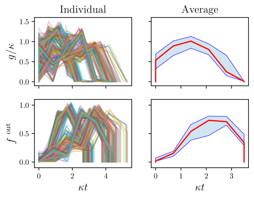
In the higher dimensional spaces, 13-d for piecewise linear (PWL) coupling and measurement functions, and 19-d when the detuning is also optimised, BO has greater difficultly exploring the space, possibly simply because of the vastness, but also indicating that at least some of these dimensions contain local maxima. This is manifested in the wider spread of seen in Fig. 3 for the higher dimensional search spaces. This is further illustrated in Fig. 6, which shows the solutions for and found by BO. The ‘Average’ plots indicate the common features of the optimised pulses, however, there is clearly significant variation in the solutions. The fact that they all produce high levels of squeezing indicates near degeneracy, as seen in the 2-d space.
Typically, the number of steps (function evaluations) allowed to BO must scale with the dimension of the space. However, the topography is also a factor – more traps means more steps are needed – so determining the ideal number of steps for some optimisation is non-trivial. A summary of the number of BO phase steps used is given in Table 2. BO produces very similar results using half as many steps, but with a wider distribution of results. Tests with many more steps did not improve the consistency of the outcome significantly. In comparison, using the gradient-based algorithm (with approximated gradients) the (two-variable) optimisation of the constant pulse performed similarly well with the same number of function evaluations. Whereas, for the PWL cases, the results were less consistent, and required over 2000 function evaluations on average. This supports the idea of local traps in the optimisation landscape that BO negotiates with some success.
The traps seem to exist in the coupling parameter dimensions. When optimising only the measurement function in repeated attempts, the maximal has a very narrow distribution – see Fig. 3, ‘ only’ dataset. The minimum, mean, maximum are are . Correspondingly we find a distinct solution for illustrated in Fig. 7.
B.4 High temperature bath and numerical stability
The two-mode generalised squeezing achievable through optimisation of the driving pulse parameters is shown in Fig. 8 for a set of reheating rates arising from bath temperatures in the range with fixed mechanical damping . The optimal squeezing for each reheating rate is shown for the top-hat pulse, in which the optimisation variables are coupling strength and duration only. The plots allows a comparison between the exact solution, which requires the rotating wave approximation (RWA), and the numerical solution, which does not use the RWA for computing the covariance matrix . The squeezing achieved through optimisation of the piecewise linear (PWL) parameters of coupling pulse strength and detuning profiles is also shown for comparison.
We note that in the experimentally interesting range the PWL shaped pulse out-performs the top-hat pulse. In the low heating range we would expect that the PWL pulse would be at least as good as the top-hat pulse, as the constant coupling strength with fixed detuning solution is within the parameter space of the PWL pulse optimisation landscape. However, we notice that the squeezing generated by the PWL pulse solution is generally lower in this low heating range, which is symptomatic of the difficultly that Bayesian Optimisation (BO) has in navigating this parameter space. This additional difficulty at these temperatures is most likely due to the optimal solution being located at the bounds of the coupling strength dimension, that is , which we have found that BO is less likely to locate than maxima within the bounds of the search space. The reheating limit , beyond which two-mode squeezing would be unmeasurable, is not extended by increasing the search space to include the extra dimensions provided by PWL shaping of the coupling strength and detuning .
In the high heating range, for the oscillator initially in thermal equilibrium , the elements of the covariance matrix become very large, and this results in numeric instability when using the numerical solver. This could likely be avoided through tighter setting of the ODE solver tolerances. It is also avoided through simulating based on the oscillator being cooled before the squeeze driving pulse is applied. For the reheating range used here we find that initial cooling down to the phonon level is sufficient for numerical stability. Note that this has no effect of the level of squeezing achievable, except at the extremely low bath temperatures , which are not achievable in any experiment and hence not considered.
There is a significant divergence of the squeezing predicted by the numerical and exact solving methods for the top-hat pulse in the both the low and high reheating range. The computations of the covariance matrix differ due to the necessary use of the RWA to calculate an exact solution. Divergence between squeezing values due to the RWA was illustrated in Fig. 5, for a fixed reheating rate and varying coupling strength . We see here that this divergence is also reheating rate dependent. The low reheating range is inaccessible in the lab. The long tail of very low squeezing at high temperatures is an interesting and unexpected feature that only appears for low frequency oscillations . It could potentially be exploited to obtain measurable squeezing if extremely high coupling could be achieved, as mentioned in Section IV.1. The numerical and exact solver squeezing values converge for fast oscillations, validated with high oscillator frequency (up to ). All results presented in the main part of the manuscript are based on the numerical solver, as this provides a more accurate model of the system by including the faster rotating terms in the drift matrix.
In Section IV we reported the two-mode squeezing levels achievable at the high reheating rate for the different optimisation variable scenarios. These high temperature bath results are presented together in Fig. 9. We see the same relationship as for the state-of-the-art experimentally achievable reheating rate , which is used for the comparable datasets presented in Fig. 3. That is, the average squeezing increases as extra dimensions are added to the search space. Note that, at this reheating rate, stable numerical evolution of the covariance matrix is possible at a higher (than was needed at the highest reheating rates used in Fig. 8) initial oscillator phonon level .
B.5 Optimisation of detection angles
a.) Exact, RWA
b.) Numeric, strong coupling
c.) Cooled oscillator
Section IV.4 reports that numerical optimisation can be used to determine the homodyne measurement angles that would allow direct measurement of equivalent to , and hence be used to calculate the two-mode squeezing . The simulations find that the occupation of the mechanical oscillator must be much lower than environmental equilibrium () for the optimisation algorithm to be able to effectively navigate the optimisation landscape and reliably find the values that give equivalent to (found through eigendecomposition).
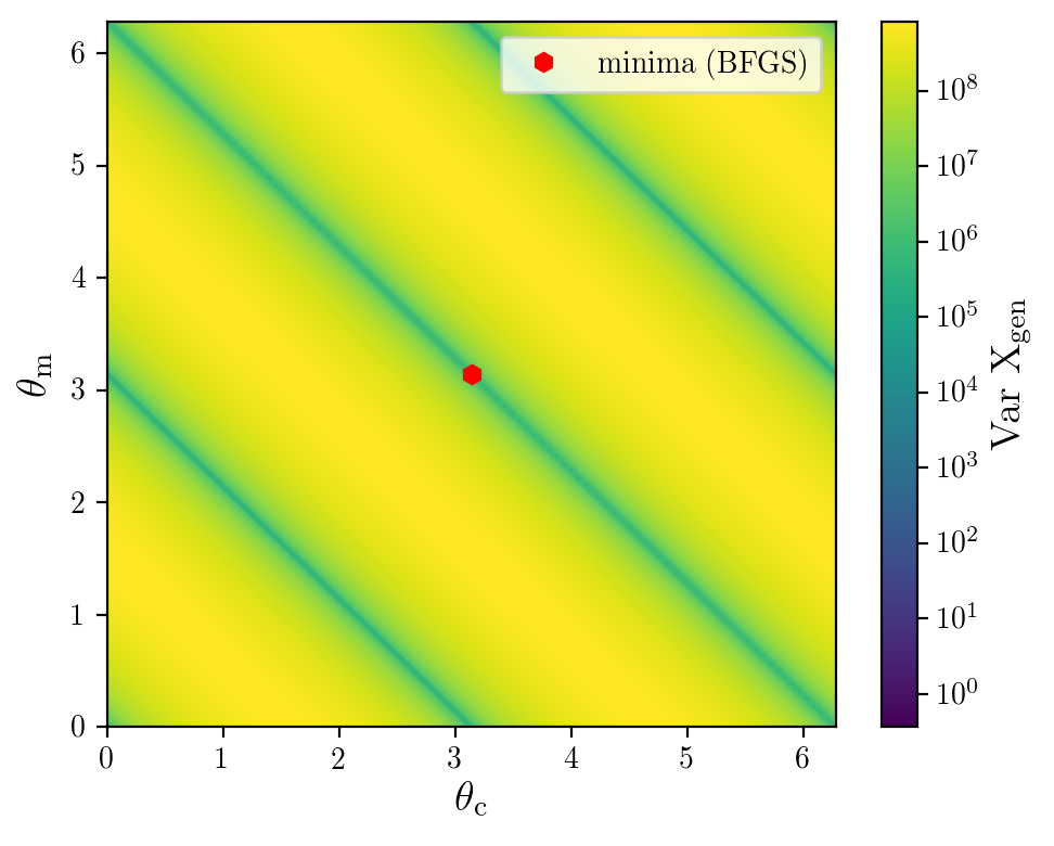
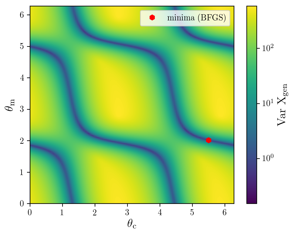
The simulations compute the covariance matrix , either analytically or numerically, as described in Appendix B.1, and so is calculated using Eq. (20). As and can be derived, then a Newton-Raphson based method is efficient for determining the optimal . In this case the ‘Newton conjugate gradient’ method in scipy.optimize is used. Hence the optimisation landscape can be reduced to two dimensions and can be visualised in the contour plots of Fig. 10.
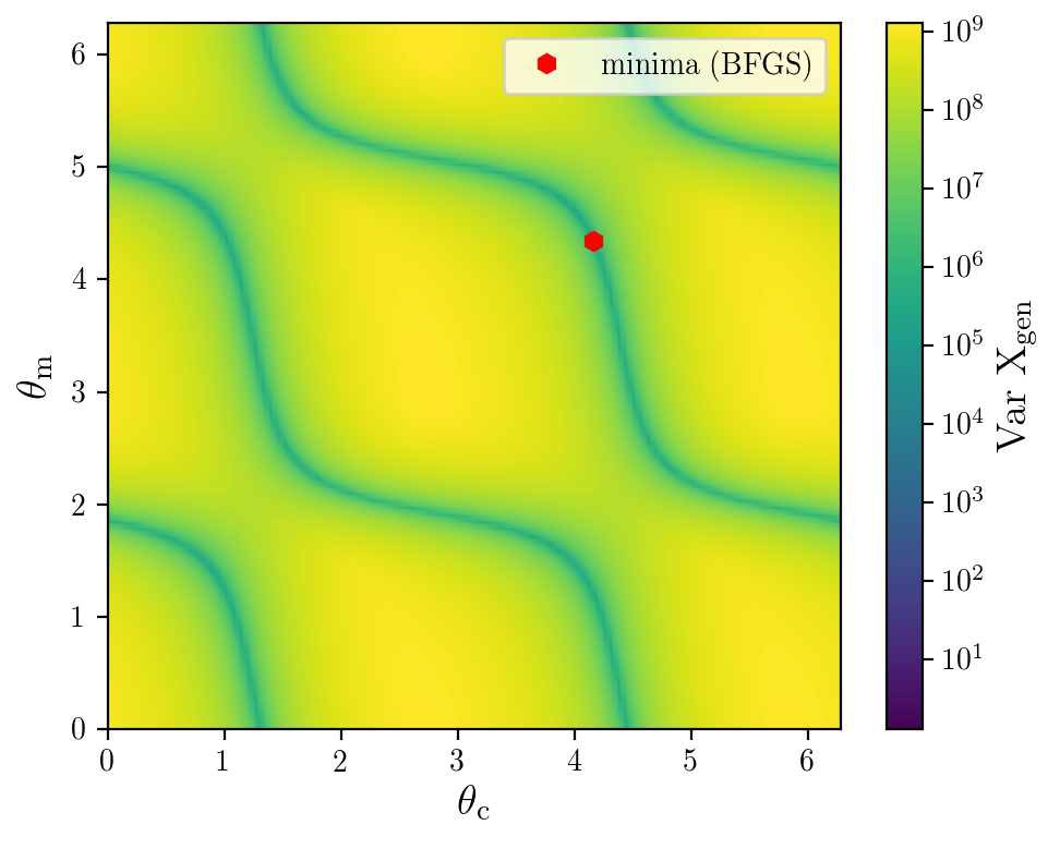
For covariance matrices computed using the analytical method, which uses the rotating wave approximation (RWA), the landscape with respect to the detection angles appears uniform, such as in example Fig. 10.a), in that it is found invariant (within numerical error) for , which is confirmed by optimisation finding the same when optimising over 1 angle () or both independently. The covariance matrices generated by numerically solving the Lyapunov equation Eq. (16) are not found to have a uniform , such as in the example Fig. 10.b). This non-uniformity is most likely also to appear in covariance matrices measured through experiment, as the numerical solution is a more accurate model of the physical system, because it does not use the RWA.
The form of Eq. (18) implies that solutions to a minimisation of Eq. (18) would be periodic in . This is illustrated in the contour plots of Fig. 10. There is nothing obvious in the mathematics that shows the quadrature detection angles to be bounded other than as , however the physical interpretation implies that the upper bound should be . The periodicity visible in Fig. 10 confirms this physical interpretation.
In the non-uniform cases the dark trenches in Fig. 10, indicating the lowest values of , are not uniformly deep, and the optimal solution is only found at specific locations. In the thermal equilibrium case (panel b.), due to the narrowness of the trench and the relative height of the surrounding landscape, neither gradient-based nor Bayesian type optimisation is reliable in locating the minimum value of corresponding to the value of . Physically this means that the sensitivity of the squeezing measure to small variations in would make it practically impossible to locate values for the angles that would indicate the representative value of .
The sensitivity of to variations in the detection angles is reduced by cooling the oscillator prior to application of the coupling pulse. The example Fig. 10.c) is from a covariance matrix generated using the same parameters as used in b.), except that the initial occupation of the oscillator is set lower . It can clearly be seen from the plot that the trenches are much wider. In this case the optimisation algorithm is able to reliably find the angles which give the smallest eigenvalue, that is . Cooling of the oscillator to these levels and beyond is possible in some experimental setups, and would be necessary in order to use this method to measure the two-mode squeezing.
Small changes in produce large variations in , and hence we find they cannot be optimised in the same space as the driving pulse parameter variables, and so optimisation of is performed in a separate process. In tests optimising , using both the square and PWL coupling pulse, in all but a few isolated cases, the optimal detection angles could be determined for the covariance matrix at each step of the algorithm. For these tests a gradient-based algorithm was used to determine , as it is more efficient to compute. Approximately 200 function evaluations gives a solution to satisfactory precision. In an experimental set up, Bayesian optimisation may perform better if there are limits on the precision to which the angles can be set, or there is significant variance in the measurement output.
B.6 Optimisation with noisy controls
The results for optimisation when the coupling pulse controls are noisy are given in Section IV.5. The coupling is piecewise linear (PWL) parameterised. To model the potential noise in attempting to drive this coupling, each of the PWL parameters have some Gaussian distributed value added to them. For the results presented, the Gaussian parameters are mean zero and standard deviation . The noise is truncated at standard deviation to exclude the possibility of negative coupling.
The noise is added at each step of the optimisation algorithm. That is, each set of parameters suggested by BO has noise added to them before the figure of merit is calculated. The final squeezing value however is calculated without noise, as this would obscure the result. This is illustrated in Fig. 11, which shows the distribution of for 2000 repetitions using the best parameter set found through optimisation with noise added as described above. As would be expected, results are distributed around , which is the value of with computed without control noise.
References
- D. et al. (2018) Braun D., Adesso G., Benatti F., Floreanini R., Marzolino U., Mitchell M. W., and Pirandola S., “Quantum-enhanced measurements without entanglement,” Rev. Mod. Phys. 90, 035006 (2018).
- N. et al. (2002) Gisin N., Ribordy G., Tittel W., and Zbinden H., “Quantum cryptography,” Rev. Mod. Phys. 74, 145 (2002).
- Deutsch (1985) D. Deutsch, “Quantum theory, the Church–Turing principle and the universal quantum computer,” Proceedings of the Royal Society of London. A. Mathematical and Physical Sciences 400, 97–117 (1985).
- Jozsa and Linden (2003) Richard Jozsa and Noah Linden, “On the role of entanglement in quantum-computational speed-up,” Proceedings of the Royal Society of London. Series A: Mathematical, Physical and Engineering Sciences 459, 2011–2032 (2003).
- Boyer et al. (2017) Michel Boyer, Aharon Brodutch, and Tal Mor, “Entanglement and deterministic quantum computing with one qubit,” Physical Review A 95, 022330 (2017).
- de Groot and Mazur (1962) S.R. de Groot and P. Mazur, Non-Equilibrium Thermodynamics (North-Holland, Amsterdam, 1962).
- Oppenheim et al. (2002) Jonathan Oppenheim, Michał Horodecki, Paweł Horodecki, and Ryszard Horodecki, “Thermodynamical approach to quantifying quantum correlations,” Phys. Rev. Lett. 89, 180402 (2002).
- Perarnau-Llobet et al. (2015) Martí Perarnau-Llobet, Karen V. Hovhannisyan, Marcus Huber, Paul Skrzypczyk, Nicolas Brunner, and Antonio Acín, “Extractable work from correlations,” Phys. Rev. X 5, 041011 (2015).
- Modi et al. (2012) Kavan Modi, Aharon Brodutch, Hugo Cable, Tomasz Paterek, and Vlatko Vedral, “The classical-quantum boundary for correlations: Discord and related measures,” Rev. Mod. Phys. 84, 1655–1707 (2012).
- Chen et al. (2014a) Moran Chen, Nicolas C. Menicucci, and Olivier Pfister, “Experimental Realization of Multipartite Entanglement of 60 Modes of a Quantum Optical Frequency Comb,” Physical Review Letters 112, 120505 (2014a).
- Cai et al. (2017) Y. Cai, J. Roslund, G. Ferrini, F. Arzani, X. Xu, C. Fabre, and N. Treps, “Multimode entanglement in reconfigurable graph states using optical frequency combs,” Nature Communications 8, 1–9 (2017).
- Zhong et al. (2018) Han-Sen Zhong, Yuan Li, Wei Li, Li-Chao Peng, Zu-En Su, Yi Hu, Yu-Ming He, Xing Ding, Weijun Zhang, Hao Li, Lu Zhang, Zhen Wang, Lixing You, Xi-Lin Wang, Xiao Jiang, Li Li, Yu-Ao Chen, Nai-Le Liu, Chao-Yang Lu, and Jian-Wei Pan, “12-Photon Entanglement and Scalable Scattershot Boson Sampling with Optimal Entangled-Photon Pairs from Parametric Down-Conversion,” Physical Review Letters 121, 250505 (2018).
- Asavanant et al. (2019) Warit Asavanant, Yu Shiozawa, Shota Yokoyama, Baramee Charoensombutamon, Hiroki Emura, Rafael N. Alexander, Shuntaro Takeda, Jun-ichi Yoshikawa, Nicolas C. Menicucci, Hidehiro Yonezawa, and Akira Furusawa, “Generation of time-domain-multiplexed two-dimensional cluster state,” Science 366, 373–376 (2019).
- Madjarov et al. (2020) Ivaylo S. Madjarov, Jacob P. Covey, Adam L. Shaw, Joonhee Choi, Anant Kale, Alexandre Cooper, Hannes Pichler, Vladimir Schkolnik, Jason R. Williams, and Manuel Endres, “High-fidelity control, detection, and entanglement of alkaline-earth rydberg atoms,” arXiv: (2020), 2001.04455 [physics.atom-ph] .
- Gil et al. (2014) L. I. R. Gil, R. Mukherjee, E. M. Bridge, M. P. A. Jones, and T. Pohl, “Spin squeezing in a rydberg lattice clock,” Phys. Rev. Lett. 112, 103601 (2014).
- Omran et al. (2019) A. Omran, H. Levine, A. Keesling, G. Semeghini, T. T. Wang, S. Ebadi, H. Bernien, A. S. Zibrov, H. Pichler, S. Choi, J. Cui, M. Rossignolo, P. Rembold, S. Montangero, T. Calarco, M. Endres, M. Greiner, V. Vuletić, and M. D. Lukin, “Generation and manipulation of schrödinger cat states in rydberg atom arrays,” Science 365, 570–574 (2019).
- Leibfried et al. (2004) D. Leibfried, M. D. Barrett, T. Schaetz, J. Britton, J. Chiaverini, W. M. Itano, J. D. Jost, C. Langer, and D. J. Wineland, “Toward heisenberg-limited spectroscopy with multiparticle entangled states,” Science 304, 1476–1478 (2004).
- Monz et al. (2011) Thomas Monz, Philipp Schindler, Julio T. Barreiro, Michael Chwalla, Daniel Nigg, William A. Coish, Maximilian Harlander, Wolfgang Hänsel, Markus Hennrich, and Rainer Blatt, “14-qubit entanglement: Creation and coherence,” Phys. Rev. Lett. 106, 130506 (2011).
- Friis et al. (2018) Nicolai Friis, Oliver Marty, Christine Maier, Cornelius Hempel, Milan Holzäpfel, Petar Jurcevic, Martin B. Plenio, Marcus Huber, Christian Roos, Rainer Blatt, and Ben Lanyon, “Observation of Entangled States of a Fully Controlled 20-Qubit System,” Physical Review X 8, 021012 (2018), arXiv:1711.11092 .
- Berkley et al. (2003) A. J. Berkley, H. Xu, R. C. Ramos, M. A. Gubrud, F. W. Strauch, P. R. Johnson, J. R. Anderson, A. J. Dragt, C. J. Lobb, and F. C. Wellstood, “Entangled Macroscopic Quantum States in Two Superconducting Qubits,” Science 300, 1548–1550 (2003).
- Steffen et al. (2006) Matthias Steffen, M. Ansmann, Radoslaw C. Bialczak, N. Katz, Erik Lucero, R. McDermott, Matthew Neeley, E. M. Weig, A. N. Cleland, and John M. Martinis, “Measurement of the Entanglement of Two Superconducting Qubits via State Tomography,” Science 313, 1423–1425 (2006).
- Dolde et al. (2013) F. Dolde, I. Jakobi, B. Naydenov, N. Zhao, S. Pezzagna, C. Trautmann, J. Meijer, P. Neumann, F. Jelezko, and J. Wrachtrup, “Room-temperature entanglement between single defect spins in diamond,” Nature Physics 9, 139–143 (2013).
- Wollman et al. (2015) E. E. Wollman, C. U. Lei, A. J. Weinstein, J. Suh, A. Kronwald, F. Marquardt, A. A. Clerk, and K. C. Schwab, “Quantum squeezing of motion in a mechanical resonator,” Science 349, 952–955 (2015).
- Pirkkalainen et al. (2015) J.-M. Pirkkalainen, E. Damskägg, M. Brandt, F. Massel, and M. A. Sillanpää, “Squeezing of quantum noise of motion in a micromechanical resonator,” Phys. Rev. Lett. 115, 243601 (2015).
- Riedinger et al. (2018) Ralf Riedinger, Andreas Wallucks, Igor Marinković, Clemens Löschnauer, Markus Aspelmeyer, Sungkun Hong, and Simon Gröblacher, “Remote quantum entanglement between two micromechanical oscillators,” Nature 556, 473–477 (2018), arXiv:1710.11147 .
- Ockeloen-Korppi et al. (2018) C. F. Ockeloen-Korppi, E. Damskägg, J.-M. Pirkkalainen, M. Asjad, A. A. Clerk, F. Massel, M. J. Woolley, and M. A. Sillanpää, “Stabilized entanglement of massive mechanical oscillators,” Nature 556, 478–482 (2018), arXiv:1711.01640 .
- Palomaki et al. (2013) T. A. Palomaki, J. D. Teufel, R. W. Simmonds, and K. W. Lehnert, “Entangling Mechanical Motion with Microwave Fields,” Science 342, 710–713 (2013).
- Hofer et al. (2011) Sebastian G. Hofer, Witlef Wieczorek, Markus Aspelmeyer, and Klemens Hammerer, “Quantum entanglement and teleportation in pulsed cavity optomechanics,” Physical Review A 84, 052327 (2011), arXiv:1108.2586 .
- Mockus (1989) Jonas Mockus, Bayesian Approach to Global Optimization : Theory and Applications (Springer Netherlands, Dordrecht, 1989).
- Judson and Rabitz (1992) Richard S. Judson and Herschel Rabitz, “Teaching lasers to control molecules,” Physical Review Letters 68, 1500–1503 (1992).
- Phan and Rabitz (1997) M Q Phan and H Rabitz, “Learning control of quantum-mechanical systems by laboratory identification of effective input-output maps,” Chemical Physics 217, 389 (1997).
- Phan and Rabitz (1999) Minh Q. Phan and Herschel Rabitz, “A self-guided algorithm for learning control of quantum-mechanical systems,” Journal of Chemical Physics 110, 34–41 (1999).
- Weinacht et al. (2001) T.C. Weinacht, R. Bartels, S. Backus, P.H. Bucksbaum, B. Pearson, J.M. Geremia, H. Rabitz, H.C. Kapteyn, and M.M. Murnane, “Coherent learning control of vibrational motion in room temperature molecular gases,” Chemical Physics Letters 344, 333–338 (2001).
- Zhu and Rabitz (2003) Wusheng Zhu and Herschel Rabitz, “Closed loop learning control to suppress the effects of quantum decoherence,” The Journal of Chemical Physics 118, 6751–6757 (2003).
- Cardoza et al. (2005) David Cardoza, Carlos Trallero-Herrero, Florian Langhojer, Herschel Rabitz, and Thomas Weinacht, “Transformations to diagonal bases in closed-loop quantum learning control experiments,” The Journal of Chemical Physics 122, 124306 (2005).
- Chen et al. (2014b) Chunlin Chen, Daoyi Dong, Ruixing Long, Ian R. Petersen, and Herschel A. Rabitz, “Sampling-based learning control of inhomogeneous quantum ensembles,” Physical Review A - Atomic, Molecular, and Optical Physics 89, 023402 (2014b), arXiv:1308.1454 .
- Egger and Wilhelm (2014) D. J. Egger and F. K. Wilhelm, “Adaptive Hybrid Optimal Quantum Control for Imprecisely Characterized Systems,” Physical Review Letters 112, 240503 (2014).
- Kelly et al. (2014) J. Kelly, R. Barends, B. Campbell, Y. Chen, Z. Chen, B. Chiaro, A. Dunsworth, A. G. Fowler, I. C. Hoi, E. Jeffrey, A. Megrant, J. Mutus, C. Neill, P. J.J. O’Malley, C. Quintana, P. Roushan, D. Sank, A. Vainsencher, J. Wenner, T. C. White, A. N. Cleland, and John M. Martinis, “Optimal quantum control using randomized benchmarking,” Physical Review Letters 112, 240504 (2014), arXiv:1403.0035 .
- Kelly et al. (2016) J. Kelly, R. Barends, A. G. Fowler, A. Megrant, E. Jeffrey, T. C. White, D. Sank, J. Y. Mutus, B. Campbell, Yu Chen, Z. Chen, B. Chiaro, A. Dunsworth, E. Lucero, M. Neeley, C. Neill, P. J.J. O’Malley, C. Quintana, P. Roushan, A. Vainsencher, J. Wenner, and John M. Martinis, “Scalable in situ qubit calibration during repetitive error detection,” Physical Review A 94, 1–8 (2016), arXiv:1603.03082 .
- Dive et al. (2018) Benjamin Dive, Alexander Pitchford, Florian Mintert, and Daniel Burgarth, “In situ upgrade of quantum simulators to universal computers,” Quantum 2, 80 (2018), arXiv:1701.01723 .
- Johnson et al. (2017) Peter D. Johnson, Jonathan Romero, Jonathan Olson, Yudong Cao, and Alán Aspuru-Guzik, “QVECTOR: an algorithm for device-tailored quantum error correction,” (2017), arXiv:1711.02249 .
- Delić et al. (2020) Uroš Delić, Manuel Reisenbauer, Kahan Dare, David Grass, Vladan Vuletić, Nikolai Kiesel, and Markus Aspelmeyer, “Cooling of a levitated nanoparticle to the motional quantum ground state,” Science 367, 892–895 (2020), arXiv:1911.04406 .
- Rakhubovsky et al. (2020) Andrey A. Rakhubovsky, Darren W. Moore, Uroš Delić, Nikolai Kiesel, Markus Aspelmeyer, and Radim Filip, “Detecting nonclassical correlations in levitated cavity optomechanics,” arXiv:2003.09894 [quant-ph] (2020), arXiv:2003.09894 [quant-ph] .
- Genes et al. (2008) C. Genes, A. Mari, P. Tombesi, and D. Vitali, “Robust entanglement of a micromechanical resonator with output optical fields,” Physical Review A 78, 032316 (2008).
- Kiesewetter et al. (2014) S. Kiesewetter, Q. Y. He, P. D. Drummond, and M. D. Reid, “Scalable quantum simulation of pulsed entanglement and Einstein-Podolsky-Rosen steering in optomechanics,” Physical Review A 90, 043805 (2014).
- Rakhubovsky and Filip (2015) Andrey A. Rakhubovsky and Radim Filip, “Robust entanglement with a thermal mechanical oscillator,” Physical Review A 91, 062317 (2015).
- Lin and He (2015) Qing Lin and Bing He, “Optomechanical entanglement under pulse drive,” Optics Express 23, 24497 (2015), arXiv:1506.02452 .
- Rudolph et al. (2020) Henning Rudolph, Klaus Hornberger, and Benjamin A. Stickler, “Entangling levitated nanoparticles by coherent scattering,” Physical Review A 101, 011804 (2020), arXiv:2001.05769 .
- Lin et al. (2020) Qing Lin, Bing He, and Min Xiao, “Entangling Two Macroscopic Mechanical Resonators at High Temperature,” Physical Review Applied 13, 034030 (2020).
- Clarke et al. (2019) J. Clarke, P. Sahium, K. E. Khosla, I. Pikovski, M. S. Kim, and M. R. Vanner, “Generating mechanical and optomechanical entanglement via pulsed interaction and measurement,” (2019), arXiv:1910.09603 .
- Aspelmeyer et al. (2014) Markus Aspelmeyer, Tobias J. Kippenberg, and Florian Marquardt, “Cavity optomechanics,” Reviews of Modern Physics 86, 1391–1452 (2014), arXiv: 1303.0733.
- Bowen and Milburn (2015) Warwick P. Bowen and Gerard J. Milburn, Quantum Optomechanics (CRC Press, 2015) google-Books-ID: YZDwCgAAQBAJ.
- Genes et al. (2009) C. Genes, A. Mari, D. Vitali, and P. Tombesi, “Quantum Effects in Optomechanical Systems,” in Advances In Atomic, Molecular, and Optical Physics, Vol. 57, edited by Ennio Arimondo, Paul R. Berman, and C. C. Lin (Academic Press, 2009) pp. 33–86, http://arxiv.org/abs/0901.2726.
- Rakhubovsky et al. (2019) Andrey A Rakhubovsky, Darren W Moore, and Radim Filip, “Nonclassical states of levitated macroscopic objects beyond the ground state,” Quantum Science and Technology 4, 024006 (2019), arXiv:1810.12178 .
- Romero-Isart et al. (2011) O. Romero-Isart, A. C. Pflanzer, M. L. Juan, R. Quidant, N. Kiesel, M. Aspelmeyer, and J. I. Cirac, “Optically levitating dielectrics in the quantum regime: Theory and protocols,” Physical Review A 83, 013803 (2011), arXiv:1010.3109 .
- Law (1995) C. K. Law, “Interaction between a moving mirror and radiation pressure: A Hamiltonian formulation,” Physical Review A 51, 2537–2541 (1995).
- Gonzalez-Ballestero et al. (2019) C. Gonzalez-Ballestero, P. Maurer, D. Windey, L. Novotny, R. Reimann, and O. Romero-Isart, “Theory for cavity cooling of levitated nanoparticles via coherent scattering: Master equation approach,” Physical Review A 100, 013805 (2019), arXiv:1902.01282 .
- Braginsky et al. (1970) V. B. Braginsky, Manukin, A. B., and Tikhonov, M. Yu., “Investigation of Dissipative Ponderomotive Effects of Electromagnetic Radiation,” Soviet Journal of Experimental and Theoretical Physics 31, 829 (1970).
- Giovannetti and Vitali (2001) Vittorio Giovannetti and David Vitali, “Phase-noise measurement in a cavity with a movable mirror undergoing quantum Brownian motion,” Physical Review A 63, 023812 (2001).
- Gardiner and Collett (1985) C. W. Gardiner and M. J. Collett, “Input and output in damped quantum systems: Quantum stochastic differential equations and the master equation,” Physical Review A 31, 3761–3774 (1985).
- Takase et al. (2019) Kan Takase, Masanori Okada, Takahiro Serikawa, Shuntaro Takeda, Jun-ichi Yoshikawa, and Akira Furusawa, “Complete temporal mode characterization of non-Gaussian states by a dual homodyne measurement,” Physical Review A 99, 033832 (2019), arXiv:1901.04669 .
- Simon et al. (1994) R. Simon, N. Mukunda, and Biswadeb Dutta, “Quantum-noise matrix for multimode systems: U(n) invariance, squeezing, and normal forms,” Physical Review A 49, 1567–1583 (1994).
- Filip (2010) Radim Filip, “Squeezing restoration by a noisy probe from a classically correlated environment,” Physical Review A 81, 032330 (2010).
- Vanner et al. (2015) M. R. Vanner, I. Pikovski, and M. S. Kim, “Towards Optomechanical Quantum State Reconstruction of Mechanical Motion,” Annalen der Physik 527, 15–26 (2015), arXiv: 1406.1013.
- Rakhubovsky and Filip (2017) Andrey A. Rakhubovsky and Radim Filip, “Photon-phonon-photon transfer in optomechanics,” Scientific Reports 7, 46764 (2017), arXiv: 1701.04986.
- Wigley et al. (2016) P. B. Wigley, P. J. Everitt, A. van den Hengel, J. W. Bastian, M. A. Sooriyabandara, G. D. McDonald, K. S. Hardman, C. D. Quinlivan, P. Manju, C. C. N. Kuhn, I. R. Petersen, A. N. Luiten, J. J. Hope, N. P. Robins, and M. R. Hush, “Fast machine-learning online optimization of ultra-cold-atom experiments,” Sci. Rep. 6, 25890 (2016).
- Zhu et al. (2018) D. Zhu, N. M. Linke, M. Benedetti, K. A. Landsman, N. H. Nguyen, C. H. Alderete, A. Perdomo-Ortiz, N. Korda, A. Garfoot, C. Brecque, L. Egan, O. Perdomo, and C. Monroe, “Training of Quantum Circuits on a Hybrid Quantum Computer,” arXiv:1812.08862 (2018).
- Henson et al. (2018) Bryce M. Henson, Dong K. Shin, Kieran F. Thomas, Jacob A. Ross, Michael R. Hush, Sean S. Hodgman, and Andrew G. Truscott, “Approaching the adiabatic timescale with machine learning,” Proceedings of the National Academy of Sciences of the United States of America 115, 13216–13221 (2018).
- Nakamura et al. (2019) Ippei Nakamura, Atsunori Kanemura, Takumi Nakaso, Ryuta Yamamoto, and Takeshi Fukuhara, “Non-standard trajectories found by machine learning for evaporative cooling of 87 Rb atoms ,” Optics Express 27, 20435 (2019).
- Mukherjee et al. (2020) Rick Mukherjee, Frederic Sauvage, Harry Xie, Robert Löw, and Florian Mintert, “Preparation of ordered states in ultra-cold gases using bayesian optimization,” (2020), arXiv:2001.03520 [quant-ph] .
- Sauvage and Mintert (2019) Frederic Sauvage and Florian Mintert, “Optimal quantum control with poor statistics,” arXiv e-prints , arXiv:1909.01229 (2019), arXiv:1909.01229 [quant-ph] .
- Brochu et al. (2010) Eric Brochu, Vlad M Cora, and Nando De Freitas, “A tutorial on bayesian optimization of expensive cost functions, with application to active user modeling and hierarchical reinforcement learning,” arXiv:1012.2599 (2010).
- Snoek et al. (2012) Jasper Snoek, Hugo Larochelle, and Ryan P Adams, “Practical bayesian optimization of machine learning algorithms,” in Advances in neural information processing systems (2012) pp. 2951–2959.
- Frazier (2018) Peter I Frazier, “A tutorial on bayesian optimization,” arXiv:1807.02811 (2018).
- Shahriari et al. (2015) Bobak Shahriari, Kevin Swersky, Ziyu Wang, Ryan P Adams, and Nando De Freitas, “Taking the human out of the loop: A review of bayesian optimization,” Proceedings of the IEEE 104, 148–175 (2015).
- Williams and Rasmussen (2006) Christopher KI Williams and Carl Edward Rasmussen, Gaussian processes for machine learning, Vol. 2 (MIT press Cambridge, MA, 2006).
- Sommer et al. (2020) Andrés de los Ríos Sommer, Nadine Meyer, and Romain Quidant, “Strong Optomechanical Coupling at Room Temperature by Coherent Scattering,” arXiv:2005.10201 [physics, physics:quant-ph] (2020), arXiv:2005.10201 [physics, physics:quant-ph] .
- Monteiro et al. (2013) T. S. Monteiro, J. Millen, G. A. T. Pender, Florian Marquardt, D. Chang, and P. F. Barker, “Dynamics of levitated nanospheres: Towards the strong coupling regime,” New Journal of Physics 15, 015001 (2013).
- Hempston et al. (2017) David Hempston, Jamie Vovrosh, Marko Toroš, George Winstone, Muddassar Rashid, and Hendrik Ulbricht, “Force sensing with an optically levitated charged nanoparticle,” Applied Physics Letters 111, 133111 (2017), arXiv:1706.09774 .
- Pontin et al. (2018) A. Pontin, L. S. Mourounas, A. A. Geraci, and P. F. Barker, “Levitated optomechanics with a fiber Fabry–Perot interferometer,” New Journal of Physics 20, 023017 (2018), arXiv:1706.10227 .
- Meyer et al. (2019) Nadine Meyer, Andrés de los Rios Sommer, Pau Mestres, Jan Gieseler, Vijay Jain, Lukas Novotny, and Romain Quidant, “Resolved-Sideband Cooling of a Levitated Nanoparticle in the Presence of Laser Phase Noise,” Physical Review Letters 123, 153601 (2019), arXiv:1907.02741 .
- Meenehan et al. (2014) Seán M. Meenehan, Justin D. Cohen, Simon Gröblacher, Jeff T. Hill, Amir H. Safavi-Naeini, Markus Aspelmeyer, and Oskar Painter, “Silicon optomechanical crystal resonator at millikelvin temperatures,” Physical Review A 90, 011803 (2014).
- Nielsen et al. (2017) William Hvidtfelt Padkær Nielsen, Yeghishe Tsaturyan, Christoffer Bo Møller, Eugene S. Polzik, and Albert Schliesser, “Multimode optomechanical system in the quantum regime,” Proceedings of the National Academy of Sciences 114, 62–66 (2017), arXiv:1605.06541 .
- Shomroni et al. (2019) Itay Shomroni, Amir Youssefi, Nick Sauerwein, Liu Qiu, Paul Seidler, Daniel Malz, Andreas Nunnenkamp, and Tobias J. Kippenberg, “Two-Tone Optomechanical Instability and Its Fundamental Implications for Backaction-Evading Measurements,” Physical Review X 9, 041022 (2019), arXiv:1812.11022 .
- Barzanjeh et al. (2019) S. Barzanjeh, E. S. Redchenko, M. Peruzzo, M. Wulf, D. P. Lewis, G. Arnold, and J. M. Fink, “Stationary entangled radiation from micromechanical motion,” Nature 570, 480 (2019), arXiv:1809.05865 .
- Peterson et al. (2019) G. A. Peterson, S. Kotler, F. Lecocq, K. Cicak, X. Y. Jin, R. W. Simmonds, J. Aumentado, and J. D. Teufel, “Ultrastrong Parametric Coupling between a Superconducting Cavity and a Mechanical Resonator,” Physical Review Letters 123, 247701 (2019).
- van Loock and Furusawa (2003) P. van Loock and A Furusawa, “Detecting genuine multipartite continuous-variable entanglement,” Phys. Rev. A 67, 052315 (2003).
- Chang et al. (2020) C. W. S. Chang, C. Sabín, P. Forn-Diaz, F. Quijandría, I. Nsanzineza, G. Johansson, and C. M. Wilson, “Observation of three-photon spontaneous down-conversion in a superconducting parametric cavity,” Phys. Rev. X 10, 011011 (2020).
- Sankey et al. (2010) J. C. Sankey, C. Yang, B. M. Zwickl, A. M. Jayich, and J. G. E. Harris, “Strong and tunable nonlinear optomechanical coupling in a low-loss system,” Nature Physics 6, 707–712 (2010), arXiv:1002.4158 .
- Leijssen et al. (2017) Rick Leijssen, Giada R. La Gala, Lars Freisem, Juha T. Muhonen, and Ewold Verhagen, “Nonlinear cavity optomechanics with nanomechanical thermal fluctuations,” Nature Communications 8, ncomms16024 (2017).
- Gröblacher et al. (2015) S. Gröblacher, A. Trubarov, N. Prigge, G. D. Cole, M. Aspelmeyer, and J. Eisert, “Observation of non-Markovian micromechanical Brownian motion,” Nature Communications 6 (2015), 10.1038/ncomms8606.
- Authors (2016) The GPyOpt Authors, “GPyOpt: A Bayesian Optimization framework in Python,” http://github.com/SheffieldML/GPyOpt (2016).
- Byrd et al. (1995) Richard H. Byrd, Peihuang Lu, Jorge Nocedal, and Ciyou Zhu, “A Limited Memory Algorithm for Bound Constrained Optimization,” SIAM Journal on Scientific Computing 16, 1190–1208 (1995).
- Tange (2011) O Tange, “GNU Parallel - The Command-Line Power Tool,” ;login: The USENIX Magazine 36, 42–47 (2011).
- Russell et al. (2017) Benjamin Russell, Herschel Rabitz, and Re Bing Wu, “Control landscapes are almost always trap free: A geometric assessment,” Journal of Physics A: Mathematical and Theoretical 50, 205302 (2017), arXiv:1608.06198 .